Finding Related Tables in Data Lakes for InteractiveData Science

Yi Zhangyizhang5@cis.upenn.eduUniversity of Pennsylvania

Philadelphia, PA

Zachary G. Iveszives@cis.upenn.edu

University of PennsylvaniaPhiladelphia, PA

ABSTRACT

Many modern data science applications build on data lakes,schema-agnostic repositories of data files and data productsthat offer limited organization and management capabilities.There is a need to build data lake search capabilities intodata science environments, so scientists and analysts canfind tables, schemas, workflows, and datasets useful to theirtask at hand. We develop search and management solutionsfor the Jupyter Notebook data science platform, to enablescientists to augment training data, find potential features toextract, clean data, and find joinable or linkable tables. Ourcore methods also generalize to other settings where compu-tational tasks involve execution of programs or scripts.

CCS CONCEPTS

• Information systems→ Federated databases;

KEYWORDS

data lakes,table search,interactive data science,notebooksACM Reference Format:

Yi Zhang and Zachary G. Ives. 2020. Finding Related Tables inData Lakes for Interactive Data Science. In Proceedings of the 2020ACM SIGMOD International Conference on Management of Data(SIGMOD’20), June 14–19, 2020, Portland, OR, USA. ACM, New York,NY, USA, 16 pages. https://doi.org/10.1145/3318464.33897261 INTRODUCTION

The data lake has emerged as a schema-agnostic repositoryfor data sources and analysis results (“data products”), pro-viding centralized access to data. Typically, the data lake isan abstraction over a distributed file system or an object

Permission to make digital or hard copies of all or part of this work forpersonal or classroom use is granted without fee provided that copiesare not made or distributed for profit or commercial advantage and thatcopies bear this notice and the full citation on the first page. Copyrightsfor components of this work owned by others than the author(s) mustbe honored. Abstracting with credit is permitted. To copy otherwise, orrepublish, to post on servers or to redistribute to lists, requires prior specificpermission and/or a fee. Request permissions from permissions@acm.org.SIGMOD’20, June 14–19, 2020, Portland, OR, USA© 2020 Copyright held by the owner/author(s). Publication rights licensedto ACM.ACM ISBN 978-1-4503-6735-6/20/06. . . $15.00https://doi.org/10.1145/3318464.3389726

store. Data lakes offer strong data access benefits, but theygenerally do little to help a user find the most relevant data,understand relationships among data products, or integrateheterogeneous data sources or products.Data lakes are used in many settings across the enter-

prise and within data science. We believe data lake manage-ment [32] becomes especially necessary in collaborative datascience settings, as well as those in which data processingmethodologies are changing. A folder/file hierarchy is in-adequate for tracking data that is updated across versions,processed across (often similar) computational stages in aworkflow, used to train machine learning classifiers, andanalyzed by users. Data lakes were developed to promotereuse of data (and associated workflows) — but if users areunaware of what is available, or unable to trust what theyfind, they end up reinventing their own schemas, importprocesses, and cleaning processes. This not only leads toinefficiencies and redundant work, but also inconsistencyin data processing, irregularity in data representation, andchallenges in maintainability.

Just as good software engineering promotesmodular, main-tainable, and reusable software components, we need waysof promoting reusable units of data and processing. Towardsthis over-arching goal, we seek to help users find seman-tically related datasets to facilitate common data analyticstasks. Our work addresses interactive, “human-in-the-loop”settings in which data scientists are undertaking data discov-ery, wrangling, cleaning, and analysis tasks. We develop ageneral framework for supporting multiple measures of tablerelatedness, and build upon prior techniques developed forlooking at data-value and data-domain overlap to find union-able [33] and joinable [9, 13, 45] tables, to find mappings tocommon schemas [19] and to profile data to find joinabletables [9, 13]. Juneau additionally considers the context andintent of the user — by searching over the provenance of dataresources, and by allowing a user to specify what type oftask they are performing.We focus in this paper on tabular and “shallow” hierar-

chical data that can be imported into (possibly non-first-normal-form) relations: CSVs, structured files, external webresources, and R and Pandas dataframes. We hypothesizethat during interactive data science tasks, users often want

to search the data lake, not only by keyword, but using atable, to find other related tables. Our implemented query-by-table framework incorporates specialized relevance-rankingcriteria to support data wrangling and training tasks.We enable searching over the inputs and outputs of data

science workflows, each comprised of discrete computationalsteps or modules. Juneau assumes workflows are speci-fied as sequences of cells within computational notebooks,hosted for multiple users on the cloud, such as Jupyter Note-book/JupyterLab, Apache Zeppelin, or RStudio. (Our workgeneralizes to shell scripts or computational workflow sys-tems [18, 31, 34], and it builds upon a recent demo [44] tofocus on effective ranking.) We further assume that the out-put of eachmodule should be stored in a data lakewemanage,alongside its provenance [8]. As the user works with data,Juneau helps them find additional resources:

Augmenting training/validation data. Often, data from thesame or related sources is captured in multiple sessions (per-haps by multiple users). Given a table from one such session,a data scientist may wish to augment his or her data, to forma bigger training or validation set for machine learning.

Linking data. Records in one database may have identifiersreferencing entries in another database. Joining on theselinks brings in additional fields that may be useful to theuser or to a machine learning algorithm. It can be helpful forusers to know about such links that are implicit in the data.

Extracting machine learning features. Data scientists oftenseek additional/alternative features for a given data instance.In a collaborative setting, one data scientist may performspecific feature engineering on a data set, while another maydo it in a different way. It can be helpful for each scientist tosee alternative feature engineering possibilities.Data cleaning. Given a widely used table, a data scientist

may want to see examples of how the table is loaded orcleaned. This involves finding alternative tables derived fromthe same inputs, but perhaps with missing values filled in.

For the above scenarios, searching for tables by keywords [5,38] or row values [47, 48] is inadequate: we need a broadernotion of relatedness that may consider schema similarity,record-level overlap, description of data and workflows andsimilarity in the workflows that create or use specific tables.Tasks may involve more than searching for unionable [33]or joinable [9, 45] tables. Given the complexity of each of ourtarget tasks, we develop a general framework for composingmultiple measures of similarity, choose a tractable subset offeatures, and explore how to combine these to support newclasses of search. We make the following contributions:

• A framework for combining measures of table related-ness, which uses top-k , pruning, and approximationstrategies to return the most related tables.

• A basic set of measures of table relatedness that con-sider both row and column overlap, provenance, andapproximate matching, for multiple use cases.

• An implementation in Juneau, which extends JupyterNotebook with table search capabilities.

• Experimental validation of our methods’ accuracy andscalability, via objective measures.

Section 2 defines the table search problem and explains ourapproach. Section 3 proposes measures for table similarityand relatedness. Section 4 then develops algorithms for thesemeasures and for querying for similar tables. In Section 5we describe Juneau, which implements the query schemesproposed in this paper. We then experimentally evaluatethe Juneau implementation in Section 6, before describingrelated work in Section 7 and concluding in Section 8.

2 FINDING RELATED TABLES

As data scientists conduct their tasks, if they could easilyfind related tables (or have these recommended to them as“auto-completions”) rather than re-creating new ones, thiswould help foster many of the benefits we associate withgood software engineering. Dataset and schema reuse wouldultimately make different data analysis processes more regu-larized, and it would also provide natural ways of leveragingcommon work on cleaning, curation, and standardization.In this section, we formalize our problem, first by providingmore detail on the types of workflows and environments wetarget, then by outlining the objectives of table search.

2.1 Workflows, Notebooks, and Data

While most of our techniques apply to any general corpusof tables, we target a richer data lake environment, in whichwe can observe tasks, provenance, and updates across time.Juneau supports computational notebook software, such asJupyter Notebook [36] and its successor JupyterLab, ApacheZeppelin, and RStudio. Within this environment, users areperforming multiple computational steps over data; we con-sider the overall sequence of operations to be a (sometimesone-off and ad hoc) computational workflow. Computationalnotebook platforms directly capture workflows and data ex-ploration by interleaving source code cells (code modulesin a workflow, executed in an external interpreter or querysystem) with their outputs (in the form of rendered visualiza-tions or tabular output). Such cells typically are appended tothe notebook sequentially, preserving a type of history. Addi-tionally, cells in the computational notebook often produceside effects by modifying state (variables whose values areset, and readable by the next cell to execute) or producingtables or files (which may be read by a future cell executionthat may even occur in another notebook).

!pip install …

Collecting scikit-learn …

sms_df.head()

class sms …0 ham Go until …

# Spam Classifier Task

sms_df[‘a’].hist(…)

sms_df = pd.read_csv(…)

MarkDown

IPython

Python (no output)

Python (no output)

Python (dataframe)

Python (visualization)

def top_k…

spam.csv

Environment:!pip install

def top_k

pd.read_csv

sms_df

sms_df.head()

sms_df

sms_df[a].hist()

Figure 1: A computational notebook, data model, and workflow graph. Cells may be executed out of order, as encoded by

blue lines in the data model. The workflow graph encodes cell dataflow dependencies.

Computational notebooks are typically stored as semi-structured files, with limited data management. Notebookfiles do not fully preserve either the history of cell ver-sions and outputs, nor the order in which cells were exe-cuted — which may result in non-reproducible notebooks.However, recent projects have introduced reproducible note-books [7, 28, 37]. Juneau adopts a similar approach: it re-places the notebook software’s storage layer with a data lakestorage subsystem, and replaces the notebook documentwith a broader object model. Our storage layer facilitatesnotebook storage and retrieval. Internally it also tracks ver-sioning of the code cells, dependencies between cells thatoccur due to state sharing, and interactions between note-books and the shell or terminal via files. Figure 1 shows theinternal data model (right) of an example notebook (left).Juneau converts every notebook Ni into a workflow graph.We formalize this workflow graphWFi as a directed bipartitegraph, in which certain data object nodesDi = D1, . . . ,Dmare input to computational modules (in Jupyter, code cells),Mi = M1, . . . ,Mn, via labeled directed edges.

Each module inMi produces output data objects (set Di ),which can be inputs to other computational stages. In Juneauour focus is on data objects that can be represented in (pos-sibly non-1NF) tables. This includes input files read by thenotebook, formatted text (Markdown) cells, and outputs (files,text, images). Edges between data objects and computationalmodules are labeled with the names of the program variablesassociated with those objects.

2.2 Searching the Lake

The problem of finding related tables in a data lake has multi-ple dimensions. First, there are a variety of different “signals”for table relatedness. For instance, in some settings, we mayhave shared values or keys; in others, the data may be com-plementary and thus have no value-overlap at all. Second,

there are multiple kinds of tasks, each with different criteriafor what makes a table useful:Augmenting training or validation data: we seek tables

with similar schemata, descriptive metadata and provenance,and compatible values and datatypes — such that the tablecan be mapped as input into the machine learning algorithmbeing used. Tables that bring many new rows are preferred.Linking data: we seek data that joins with the existing

table, meaning we need to find a small number of commonschema elements with high data overlap. Tables that bringnew fields are preferred.Extracting machine learning features: machine learning

features are generally acquired by running code over thecontents of a table — the result resembles that of a join, in thatit adds columns to each row. There are two major differencesfrom the linking-data use-case: (1) the feature-extracted tablewill generally derive from a table with different provenancefrom the search table, (2) the feature-extracted table shouldtypically have a superset of the columns (and the majorityof rows) of the search table.

Data cleaning: high-ranking tables shouldmatch the schemaof the search table, and share most rows (as identified bykey) and values. The cleaned table should derive from onewith similar provenance to the search table, and generallywill have fewer null values and unique values per column.

2.3 Juneau Functionality

To support the search types described above, Juneau mustleveragemultiplemeasures for each search type, and it shouldeasily extend if new measures are proposed by future re-searchers or domain experts. Our system is given a searchtable S , a search type τ and relatedness function Relτ thatcombines multiple measures (defined in Section 3), and anindexed set of tables in a data lake. It seeks the k most related

tables. Section 4 develops (1) scalable algorithms for comput-ing our measures, (2) a top-k engine to combine them.We pri-oritize inexpensive, highly-selective measures to prune can-didate tables; then compute additional measures as needed.

Of course, any search method that must compare the con-tents of the search table against a large number of existingtables will not scale. We not only use data sketching and pro-filing techniques as in prior work [9, 13, 45], but in Section 5we develop techniques for incorporating profiling algorithmsthat can identify the semantics of certain columns by theirvalue ranges and data patterns (e.g., countries, first names).We generalize this idea to profile tables that contain certaincombinations of fields, e.g., a table of people and their IDs.We create an index from the profile tables to matching fieldsin other tables; if a search table matches against the profiletable, it can also be transitively matched to these tables.

3 MEASURES OF TABLE RELATEDNESS

The previous section gave an overview on how differentsearch classes are supported by combining multiple mea-sures. In this section, we propose basic measures of related-ness or utility sim(S,T ) between a given target table T andour current search table S . We defer implementation to thenext section. Note that the set of potential measures for ta-ble relatedness is nearly unbounded, because many domain-and data modality-specific measures might be defined fordifferent use cases. Thus, we provide a basic set of measuresfor common use cases, and the extensible Juneau frameworkcan incorporate additional measures. We divide our basicmetrics into measures of table overlap (at the row and columnlevel), useful for finding tables with schemas that augmentor join with our existing data; measures of new information(rows or columns) that favor tables that bring more infor-mation; and measures of provenance similarity that indicatesemantic relatedness between datasets. Finally, while datacleaning is a vast field that often employs domain-specifictechniques, we develop simple measures to detect the kindsof data cleaning often employed in Jupyter notebooks, whichinvolve filling in missing values.

3.1 Matching Rows and Columns

Our starting point is a measure of similarity or overlap be-tween tables that are similar, but not necessarily identical,by finding matches among sub-components (namely, rowsand columns). Intuitively, the overlap between tables may bebroken down into row- and column-level overlap. Row over-lap captures overlapping data items (or in machine learningparlance, instances); column overlap seeks to capture com-monality of schema elements. Both notions must be tolerantof small changes to schema and values.

To characterize row-level and column-level similarity be-tween a pair of tables S and T , we introduce a relation map-ping µ consisting of a key mapping and a schema mapping.Intuitively, when the pairs of attributes kS , kT in the key map-ping are equal, we have a value-based match between therows. Conversely, the schemamapping attributesmS ,mT cap-ture pairs of attributes that semantically correspond (not aspart of the key). Inspired by schema matching literature [39],we distinguish between value-based and domain-based (inthe sense of semantic types) techniques for finding relationmappings and computing table overlap.

3.1.1 Value-based Overlap. We start with a measure thecommonality between rows in the tables, which is obtainedby finding shared values in a corresponding key mapping.

Overlap with Exact Matches. For the problem of table rowoverlap, we start with a strong assumption of exact matching,which wewill ultimately relax. Given two tables S,T , we seeka mapping µ that relates tuples s ∈ S, t ∈ T .

Definition 1 (Key Mapping). If S and T overlap, we ex-pect that there is at least one candidate key kS for relation Sand kT for relation T , each containing n attributes, such thatif θkS ,kT = (kS1 = kT1 ) ∧ . . .∧ (kSn = kTn ), then we have func-tional dependency kS → S ZθkS ,kT T and kT → S ZθkS ,kT T .

We sayθkS ,kT establishes a bijective keymappingK betweenpairs kSi and kTi , for 1 ≤ i ≤ n.

Often, attributes that are not part of a candidate key arein fact mappable between pairs of relations S and T , so themapping key attributes do not fully define the relationshipbetween pairs of tuples. Moreover, even if the keys exactlymatch, the remaining attribute values may not. We thusconsider more general methods of mapping columns that donot directly overlap in value.

3.1.2 Domain-based Overlap. Domain-based overlap cap-tures the columns that are drawn from the same domain,even if they do not have overlapping values. The simplestform of domain-based overlap is to leverage similarity oflabels and compatibility of domains [39]. Another methodis to use ontologies with known instances [33]. However,ontologies often have limited coverage, and may not capturecommon patterns in the data. Therefore, we propose a moregeneral solution that we term data profiles.

Definition 2 (Data Profile). Suppose we are given aparticular domain d (where a domain might be, e.g., a name,a birthday). Given a column c , we denote the data profileof c with respect to d as Ψ(c,d), where Ψ(c,d) = ψi (c,d)i .Eachψi represents a set of features indicating column c’s valuesbelong to domaind . Given c ,d and a group of weightsω = ωi ,for each ψi , there exists a function дi , such that дi

(ψi (c,d)

)predicts the likelihood that column c has domain d . Denote

M(c,d) as the function that predicts column c is of domain d ,M(c,d) = ∑

i ωiдi(ψi (c,d)

).

We can then define the domain-based mapping as follows.

Definition 3 (Domain-based Mapping). LetD = dj bea set of domains. Given table S , we define a domain mappingΓsj ,dj , where sj is in the schema of S , dj ∈ D, and we say sjbelongs to domain dj , ifM(sj ,dj ) > τ , where τ is a threshold.

Our implementation (Section 4.2.2) relies on user-defineddata profile-detection functions called registered matchers,as well as basic value-range and uniqueness checkers, aspredictors for whether given columns map to domains.

Leveraging the domain-basedmapping, we introduce schemamapping between two tables. If we assume that the proba-bilities are independent and that we are looking for a singlecommon domain between columns, then we can further de-fine a measure of similarity between columns c and c ′ as:

MS(c, c ′) = arдmaxdM(c,d) ·M(c ′,d)We can now find correspondences between pairs of at-

tributes (sj , tj ): we assume one-to-one correspondences be-tween attributes [39], and select pairs sj , tj in decreasingorder of similarityMS(sj , tj ), only selecting each column atmost once. This yields a schema mapping:

Definition 4 (Schema Mapping). A schema mappingΓmS ,mT , where |mS ⊆ S | = |mT ⊆ T | = k , is a bijectivemapping between pairs of attributes sj ∈mS , tj ∈mT , 1 ≤ j ≤k . Initially we assume that the domains of mapped attributessj , tj are the same, which we term direct schema mappings.

3.1.3 Relation Mapping. We then define the relation map-ping, which will be a parameter to a lot of our similaritymeasures.

Definition 5 (Relation Mapping). A relation mappingbetween relations S and T , µ(S,T ) is a four-tuple(mS ,mT ,kS ,kT ) such that |mS ⊆ S | = |mT ⊆ T |, |kS ⊆ mS | =|kT ⊆ mT |, ΓmS ,mT is a schema mapping between S,T , andkS ,kT form a one-to-one key mapping K .

The culmination of these definitions yields a measure thatcan estimate the similarity between two tables:

Definition 6 (Overlapwith RelationMapping). Giventwo tables S,T and a relation mapping µ = (mS ,mT ,kS ,kT )between the tables, we define two components: row similarity,sim

µrow (S,T ), and column similarity, simµ

col (S,T ). As with [5,13], we use Jaccard similarity for each component. First, weconsider row overlap; given that kS →mS and kT →mT :

simµrow (S,T ) =

|πkS (S) ∩ πkT (T )||πkS (S) ∪ πkT (T )|

(1)

For column similarity, we consider the overlap between theschemata of S and T , denoted by vectors S, T .

simµcol (S,T ) =

|mS ||S | + |T | − |mS |

(2)

3.1.4 Relaxed Overlap Conditions. In real world datasetsthat are not controlled by a DBMS, key constraints are occa-sionally violated due to errors, data consistency issues, andjoint datasets that have not been fully de-duplicated. Thus,exact value overlap may be too strong a constraint to findkey fields and thus identify common rows. We thus relax ourconstraints to incorporate approximate key constraints, andextend the similarity metric.

Value-based Overlap with Approximate Matches. Approxi-mate functional dependencies have been heavily studied inthe database literature, with a focus on practical algorithmsfor their discovery [6, 12, 22, 24, 42]. We leverage this workto define a similarity measure (the algorithm used to detectthe approximate dependencies is orthogonal to our work).If a dependency kS → S holds, then all tuples in S with

a given value of kS must be identical. However, in an ap-proximate setting some tuples may not satisfy kS → S . Wecan collect this portion of S into a subset Sn , where for eachs ∈ Sn[kS ], there exist multiple tuples in Sn .

Definition 7 (Approximate Key Constraints). Given acandidate approximate key, kS ⊆ S , we define a factor γkS (S)to measure how well kS serves as a key of S . Adapting a metricproposed in Wang et al. [42], we measure the expected num-ber of tuples in the table associated with each value of theapproximate key, πkS (S). Note that the factor is equal to 1 if anexact functional dependency holds. Formally, γkS (S) is definedas follows: ∑

v ∈πks (S )

|σks=v (S)||πks (S)|

=|S |

|πks (S)|(3)

Thus, if kS ⊆ S , and γkS (S) ≈ 1, then we say kS is an approxi-mate key of S .

Domain-based Overlap with Approximate Matches. Just aswe may consider approximate matches for values, it is alsopossible to have a relaxed notion of domain overlap: namely,in a hierarchy or lattice of different domains, column sj maymap to domain d1, column tj may map to domain d2, and thetwo domains may relate to each other.

Definition 8 (Compound Domain Mapping). A com-pound domainmapping ΓdmS ,md

, wheremS ⊆ S,md ⊆ D, |ms | →|md |, is a mapping between attributes sj ∈ ms and domainsdj ∈md . If ∀j, Γdsj ,dj holds, we saymS belongs to a compounddomainmd . We can associate a domain precisionprecis(ms ,md )to capture how preciselymd describes the domain ofms ; theprecision of the most specific domain will be 1.0, and super-classes of this domain will have successively lower scores.

Definition 9 (Approximate Relation Mapping). Wedefine an approximate relation mapping to be a relation map-ping µ(S,T ) = (kS ,kT ,mS ,mT ), with an approximation factor,γ (S,T ), based on how closely or precisely the mapped por-tions of the relations (approximately) satisfy kS → mS andkT →mT . Formally, γµ (S,T ) is:

|πmS (S)| + |πmT (T )||πkS (S) ∪ πkT (T )|

(4)

We then compute the overlap defined in Definition 6, usingthe approximate relation mapping.

3.2 Augmenting with New Information

Table similarity measures commonality between tables, butin a variety of cases we also want to find tables that bring ina substantial amount of new data instances (rows). Therefore,we propose two metrics to measure information gain.

Definition 10 (New Row Rate). Given table S, candidatetable T , and their approximate relation mapping µ(S,T ) =(mS ,mT ,kS ,kT ), we define the new row rate of T as nrr µS (T ):

nrrµS (T ) = |πkT (T ) − πkS (S)|/|πkT (T )| (5)

Definition 11 (New Column Rate). Given table S, candi-date tableT , and their approximate relation mapping µ(S,T ) =(mS ,mT ,kS ,kT ), we define the new column rate ofT asncr µS (T ):

ncrµS (T ) = |T −mT |/|T | (6)

A complementary direction explored by Kumar et al. [29]is whether joining a table to bring in additional featuresnotably improves a classifier’s accuracy. As future work,we are interested in exploring whether their notion (whichconsiders schema constraints and VC-dimension) can beadapted to our setting in a low-overhead way.

3.3 Measures for Shared Provenance

The above similarity measures focus on matching table con-tent, i.e., instances and schema. However, tables may alsohave similarity of purpose or role: i.e., they may be producedby an identical or similar workflow (sequence of notebookcells). We begin with a variable dependency graph (as is usedin source code dependency analysis), which captures the de-pendencies among variables in the computational notebook.We extract a subgraph for each variable as its provenancegraph, and define similarity based on the edit distance be-tween provenance graphs.

Definition 12 (Variable Dependency Graph). A vari-able dependency graph of a notebook is a directed acyclic graphwith labels on edges denoted as G = (V ,E, F ). V representsthe vertices consisting of all variables detected in the notebook.F represents operations (functions) that are used on the in-put variables to generate the output variables. E(G) represents

the labeled directed edges, and for any triple ⟨u,v, l⟩ ∈ E(G),where u,v ∈ V (G), and l ∈ F (G), it means that variable u de-pends on variable v via operator l . Note that, table dependencygraph is generated by extracting the assignment relationships,variables and functions from the source code of the computa-tional notebook. To extract all of the information, we parse thesource code to an abstract syntax tree (AST).

Listing 1: Example 3.1

inFp= " t r a i n . c sv "d f _ t r a i n =pd . r e ad_c sv ( inFp )var= " S a l e P r i c e "da t a =pd . conca t ( [ d f _ t r a i n [ " GrLivArea " ] , d f _ t r a i n [ var ] ] )

Example 3.1. See Listing 1 and Figure 2. The nodes repre-sent the variables detected in the source code, including inFp,df_train, var, and data. The operators used here are func-tions such as pd.read_csv and pd.concat. The edges consistof all assignments in the source code. For example, data is out-put by running pd.concat on df_train and var. Therefore,it is connected by two edges with the same label from var,df_train respectively.

Figure 2: Variable

dependency graph

A variable dependency graph de-picts how a variable depends onand affects other variables. Buildingupon this, we introduce a variableprovenance graph for each variable.

Definition 13 (Variable Prove-nance Graph). Given a variabledependency graph G = (V ,E, F ),a variable provenance graph PG(v)where v ∈ V is a subgraph of G, which describes all variablesthat affect v and their relationships.

Definition 14 (Variable Provenance Similarity). Theprovenance similarity between two variables is defined viagraph isomorphism. GivenG = (V ,E, F ) andG ′ = (V ′,E ′, F ′),a graph isomorphism fromG toG ′ is a bijective function f : E→ E ′, s.t. ∀(u,v, l) ∈ E,∃(u ′,v ′, l ′) ∈ E ′, s.t. u ′ = f (u),v ′ =f (v) and l = l ′. Meanwhile, ∀(u ′,v ′, l ′) ∈ E ′,∃(u,v, l) ∈ E,s.t. u = f −1(u ′),v = f −1(v ′) and l ′ = l .Provenance similarity between two variables va and vb ,

where va ∈ V and vb ∈ V ′, is the graph edit distance [43], themost common measure of graph similarity, between PG(va)and PG(vb ), denoted as edt(PG(va), PG(vb )). It is the numberof edit operations in the optimal alignment that makes PG(va)reach PG(vb ). The edit operation on a graph G is an insertionor deletion of a vertex/edge or relabeling of an edge. The costs ofdifferent edit operations are assumed to be equal in this paper.

Provenance similarity between S andT , simp (S,T ), is thus:

simp (S,T ) =1

edt(PG(S), PG(T )

)+ 1

(7)

Search Class simµrow (S, T ) simµ

col (S, T ) simp (S, T ) nrr µS (T ) ncr µS (T ) ∆µ0 (S, T ) simΘ(S, T )

Augmenting Training/ Validation Data N/A ++ ++ ++ N/A N/A +Linking Tables ++ N/A N/A N/A N/A N/A +

Extracting Features ++ N/A - - N/A ++ N/A +Alternative Data Cleaning ++ ++ + N/A N/A ++ +

Table 1: How different measures correspond to different search classes.

We show an algorithm for computing provenance similarityin Section 4. Note that we only consider provenance for alldefinitions within the current notebook, and do not extendto imported packages or other files. As future work we willconsider code analysis across source files.

3.4 Other Measures

3.4.1 Description Similarity. The information of why andhow a table was derived is also important when consider-ing table similarity, especially when tables have limited rowoverlap. We consider the any descriptive information (meta-data) about the source data, as well as the workflow used toproduce the data, as a part of our similarity metrics, and weassume that they are all stored in a key-value form.

Examples of descriptive metadata are sketched in a recentvision paper [17], and may include the problem type, e.g.,classification, regression, clustering; the domain of the sourcedata, such as health care, finance, insurance; study conditions;text about workflow; etc.

We denote the description space of table S as Θ(S). Θ(S) =(θi ,vi , fi )|1 ≤ i ≤ N , where θi represents a specific typeof description, vi is the corresponding value of θi . Given an-other table T with its configuration space Θ(T ), fi measuresthe similarity between vi and v ′

i , where (θi ,vi , fi ) ∈ Θ(S)and (θi ,v ′

i , fi ) ∈ Θ(T ).Given table S,T and a description space, the description

similarity simΘ(S,T ) is defined as follows:N∑i=1

wi ∗ fi (vi ,v ′i ) (8)

wherewi is theweight for a specific feature, such that∑N

i=1wi =

1, and (θi ,vi , fi ) ∈ Θ(S) and (θi ,v ′i , fi ) ∈ Θ(T ).

3.4.2 Null Value Reduction. The number of null values in acolumn is an important signal when looking for data cleaningtasks, as a common cleaning operation is to fill in or imputemissing values. We define the measure as follows:

Definition 15 (Null Value Decrement). Given two ta-bles S,T , and the relation mapping µ(S,T ) = (mS ,mT ,kS ,kT ),the null value decrement ∆µ0 (S,T ) is:

∆µ0 (S,T ) =max0,Null

(πmS (S)

)− Null

(πmT (T )

) (9)

where Null(S) and Null(T ) represent the number of null valueentries in S and T respectively.

3.5 Composing Measures for Search

Section 2 described four typical classes of search. We now de-scribe how our primitive measures from above can facilitateranking for each search class.

3.5.1 Augmenting Training Data. Tableswith similar schemaand provenance to the search table are likely to be usefulas additional training data. Therefore, for this search class,given µ, we need a table T ∈ Σ with high sim

µcol (S,T ) and

high simp (S,T ). Meanwhile, we prefer tables that add newrows; therefore, the table should also have a high nrr

µS (T ).

Thus, Rel µ1 (S,T ) is:

ω1simµcol (S,T ) + ω2simp (S,T ) + ω3nrr

µS (T ) (10)

3.5.2 Linking Data. Rather than looking for tables that havehigh column overlap, a data scientist often needs to findtables that augment or link to the current result. This isrequires a joinable table, where we expect one-to-many (orin rare cases many-to-many) links between tuples.Again, we assume the presence of a relation mapping

µ(S,T ) = (mS ,mT ,kS ,kT ). Here, however, we expect thateither kS → S or kT → T , i.e., we can think of kS and kTas members of a key/foreign-key join. Therefore, in thefirst case, there will be a high row overlap between T andS ZkS ,kT T , which means simµ

row (T , S ZkS ,kT T ) will behigh. In the second case, the high overlap will exist betweenS and S ZkS ,kT T , which means simµ

row (S, S ZkS ,kT T ) ishigh. Formally, given tables S , T and a relation mappingµ(S,T ) = (mS ,mT ,kS ,kT ), Rel µ2 (S,T ) is:

max(sim

µrow (S, S ZθkS ,kT T ), simµ

row (T , S ZθkS ,kT T ))(11)

3.5.3 Extracting Machine Learning Features. Feature extrac-tion will typically produce tables that preserve their inputs’keys and other columns, but add more columns. We lookfor tables with high sim

µrow (S,T ) and high ncr

µS (T ) or high

simµrow (S,T ), but with low simp (S,T ). Formally, Rel µ3 is:

ω1simµrow (S,T ) + ω2ncr

µS (T ) + ω3simp (S,T ) (12)

3.5.4 Data Cleaning. Comparing with the search table, theoutput of data cleaning usually matches the schema andshares most rows, but has some data-level differences. Themost typical “signal” is a reduction in null values. Therefore,we require the table has high simµ

row (S,T ), high simµcol (S,T )

and high ∆µ0 (S,T ). Since data cleaning is usually combined

with other steps, we also require the alternative data cleaning

steps should share common provenance, which means it alsorequire a high simp (S,T ). Formally, Rel µ4 (S,T ) is as follows:

ω1simµrow (S,T ) + ω2sim

µcol (S,T ) + ω3∆

µ0 (S,T ) + ω4simp (S,T )

(13)Summary of similaritymeasures.We summarize ourmea-sures and their relative importance to each search class inTable 1. Note that we always add simΘ(S,T ), the descriptionsimilarity, to each measure: we consider it a strong indicatorif tables were created by the same organization, belong tothe same domain, or serve the same project.

4 QUERYING FOR RELATED TABLES

Leveraging the similarity metrics and search classes of theprevious section, we now develop algorithms for findingrelated tables. We must identify the best relation mappingbetween the source table S and the candidate table T (Sec-tion 4.2) and compute components of the table relatednessscore (Section 4.3). Once we have relatedness scores, wemust compute the top-k results using effective pruning andindexing strategies (Section 4.4). We start with an overviewof how ranked query processing (top-k search) works.

4.1 Overview of Top-k Search

The top-k query processing problem involves computing asfew results as possible to return the highest-scoring results.This longstanding problem in query processing typicallysets a threshold on remaining answers and returns valuesscoring above this [10, 23]. The challenge lies in using themeasures with the highest selectivity/cost trade-off to “drive”the computation and prune many potential matches; thenevaluating the remaining measures to refine our ranking.We divide our basic measures in Table 1 into two cate-

gories, based on whether they depend on finding the relationmapping µ. Typically, detecting relation mapping is moretime-consuming than other measures, i.e., simp (S,T ) andsimΘ(S,T ), since the provenance graph of a table and themetadata of the notebook or the dataset are proportionallysmall. Therefore, the relationmapping is the bottleneckwhendoing top−k search. Based on this observation, we leveragea threshold algorithmic framework to do top−k table search,whose idea is to leverage computationally efficient measuresto prune the candidate tables, minimizing computation ofthe time-consuming parts (e.g., the relation mapping).Ultimately, we must find a relation mapping between ta-

bles. To speed this up, we create indices to help quickly detecta mapping for part of a table’s schema, and then if necessary,we incrementally refine the full relation mapping detection.Since the partial relation mapping is efficient to compute, wecan also fit this staged relation mapping strategy into ourthreshold based algorithmic framework.

4.2 Detecting Relation Mappings

Most of our similarity measures require the relation mappingas input. This requires us to detect a schema mapping at thedomain-level ΓmS ,mT , and subsequently derive a set of keymappings θkS ,kT by looking at values within the mappedcolumns. In turn, finding the schema mapping involves esti-mating value-based overlap, then matching columns againstdata profiles to detect their domains.

4.2.1 Computing Value-based Overlap. We use Jaccard simi-larity between pairs of columns, to determine their overlapscore,MS(i, j):

MS(i, j) = |πsi (S) ∩ πtj (T )|/|πsi (S) ∪ πtj (T )| (14)

where si ∈ S (S is the schema for table S) and tj ∈ T . Alter-natively, we could estimate similarity using sketches or LSHbased approximation [14, 46] for scalability.

4.2.2 Computing Domain-based Overlap. Value-based over-lap is a strong signal that columns share the same domain,but sometimes different tables contain disjoint data values.As described previously, ontologies [33] are one method ofdetermining common domains, but they are often unavail-able or under-populated. To handle such cases, we proposetwo methods to identify columns’ domains.Registered Matchers. Leveraging an idea from schemamatching [39], we pre-define a series of matching functionsthat can test if the column belongs to a specific domain. Atypical example is to validate email address by regular ex-pression. In Juneau, we also allow users to register theirown matchers to match columns to specific domains. Ourimplementation, described in Section 6, supports matchersthat check columns’ data types, unique values, value ranges,and common patterns. This is generally through a combi-nation of value-range checking (e.g., for zip codes), patterndetection (e.g., for phone numbers or street addresses), andcross-checking across a dictionary (e.g., for common names).Data Profiles.More generally, we can develop algorithmsthat do data profiling to predict whether a column belongs toa domain, e.g., by testing for features as defined in Section 3:example features include columns’ data types, unique values,value ranges, and common patterns. Additionally, the outputsof the registered matchers above form additional features.

In our initial implementation of Juneau, we use Boolean-valued features, and then compute Jaccard similarity betweenthe sets of features reflected in two sets of columns. Thiscould be easily generalized to real-valued features.

We also generalize to look at co-occurring columns withinthe same schema; e.g., we may be more confident that wehave a “last name” field if there is also a “first name” field.Here, we use a Naïve Bayes model to score the probability ofc matching a column c ′, and the characteristics in this case

isψi (c) = c∗, where c∗ is the set of columns in the sametable as column c . The score is computed as follows:

p(c |ψi (c ′)

)∝ p(ψi (c ′)|c)

p(ψi (c ′)

) = ∏c∗∈ψ (c ′) p(c∗ |c)∏c∗∈ψi (c ′) p(c∗)

(15)

where p(c∗ |c) = n(c,c∗)n(c) , and p(c∗) = n(c)

N , where n(c, c∗) is thenumber of tables that contain both c and c∗, and n(c) refersto the number of tables that contain c .

4.2.3 Relation Mapping. Given matching scores betweenpairs of columns, we need to find the schemamapping ΓmS ,mT

between S andT . We find this schema mapping using integerlinear programming [26], much as in prior work [16]. For-mally, we denote xi j as the binary variable indicating if si ∈ Sis matched to tj ∈ T , according to some attribute similarityfunction that may take schema or data into account [27, 39].That is:

xi j =

1, if ΓmS ,mT [si ] = tj

0, otherwise

Here, we assume that each attribute in S can be matched toat most one attribute in T and vice versa. Thus, the objectiveis to find a mapping ΓmS ,mT satisfying the constraints thatcan maximize the matching score as follows:

argmaxΓ∑i, j

xi j MS(i, j)

s.t. xi j ∈ 0, 1, ∀i,∑j

xi j ≤ 1, ∀j,∑i

xi j ≤ 1(16)

Finally, we use a greedy algorithm proposed by Papadim-itriou [35] to get the best schema mapping.

4.2.4 Detecting keys and dependencies. For a given schemamapping, the choice of key mappings determines which rowsare mapped together, and thus it affects the relation mapping.Our goal is to find a key mapping K = (kS ,kT ) with equijoinpredicate θkS ,kT , which maximizes the table overlap.

Since table overlap includes both row and column overlap,we denote the table overlap as:

simµβ (S,T ) = βsim

µrow (S,T ) + (1 − β)simµ

col (S,T ) (17)

where parameter β allows us to adjust the weight on rowand column terms.

Next, we maximize simµβ (S,T ) (for some given parameter

β and schema mapping ΓmS ,mT ) to find the key mapping Kbetween S and T . Formally,

simµβ (S,T ) = argmaxθ ∗kS ,kT

simµβ (S,T ) (18)

Unfortunately, choosing the subset of a schema mappingas a key mapping to maximize the similarity is a variation ofthe classic, NP-hard subset-selection problem. Fortunately,the key mapping for two tables typically has a very small size,especially for linkable tables (key-foreign key joins seldom

match on more than 2-3 keys). Therefore, we do not actuallyneed to explore all subset combinations of attribute pairsfrom S andT , but limit the size of θkS ,kT to be a small integerdenoted as ks . Thus, the key mapping we are looking for is:

K : argmax(kS ,kT )st |kS |, |kT | ≤kssimµβ (S,T ) (19)

This optimization problem is tractable. We combine the cho-sen ΓmS ,mT and K to form our relation mapping µ.

4.3 Estimating Provenance Similarity

Computing provenance similarity i.e., the graph edit dis-tance between two variable provenance graphs (Section 3.3),is NP-hard [43]. In this section, we present an approxima-tion algorithm to efficiently estimate the provenance similar-ity between two tables based on their variable provenancegraphs. The basic idea of our estimation is to transform agraph structure to a multiset of star structures [43].

Star Edit Distance. To estimate the provenance similaritybetween S and T , we first derive the corresponding variableprovenance graphs, PG(S) and PG(T ), respectively. The keyidea of estimating the graph edit distance between PG(S)and PG(T ) is representing each graph to be a set of starstructures whose graph edit distance can be easily obtained.Based on the edit distances between star structures of PG(S)and PG(T ), we can estimate the lower and upper bound oftheir graph edit distance, a.k.a their provenance similarity. Inthe following part, we first introduce the star structure andthen elaborate on how to compute the edit distance betweentwo star structures.

Definition 16 (Star Structure). A star structure s is alabeled single-level, rooted tree which can be represented bya 3-tuple sr = (r ,L, f ), where r is the root vertex, L is the setof leaves. Note that edges only exist between r and any vertexin L, and no edge exists among vertices in L. f is the labelingfunction on edges.

Given PG(T ) = (V ,E, F ), we can represent it with a setof star structures, denoted as PGs (T ) = sr |r ∈ V , wheresr = (r ,L, f ) and L ⊂ E, f ⊂ F .

Definition 17 (Star Edit Distance). Given two starstructures s1 = (r1,L1, f1) and s2 = (r2,L2, f2), we denotetheir star edit distance as sdt(s1, s2). Formally,

sdt(s1, s2) = | | f1 | − | f2 | | +M(f1, f2) (20)

where M(f1, f2) = max|Ψf1 |, |Ψf2 | − |Ψf1 ∩ Ψf2 |, and Ψfrepresents the multiset of f .

Lower Bound of Edit Distance. Based on the star repre-sentation of the variable provenance graph, we introducea mapping distance between two star representations, andwe leverage it to provide a lower bound on the graph editdistance between two variable provenance graphs.

Definition 18 (Mapping Distance). Given two star rep-resentations PGs (S) and PGs (T ), assume that ϒ is a bijectivemapping between si ∈ PGs (S) and sj ∈ PGs (T ). The distanceζ between PGs(S) and PGs(T ) is

ζ (PGs (S), PGs (T )) = minϒ∑

si ∈PGs(S )sdt(si , ϒ(si )) (21)

Detecting an ϒ that can minimize the mapping distanceis also a combinatorial optimization problem, which is thesame as detecting the schema mapping described in 4.2.3.Therefore, we use the same greedy solution to find ϒ, so thatwe can compute the mapping distance efficiently.

Proposition 1. Given themapping distance between PGs (S)and PGs (T ), the provenance similarity between S ,T satisfies:

ζ (PGs (S), PGs (T )) ≤ 4 · edt(PG(S), PG(T )) (22)

Proof. Let P = (p1,p2, ...,pl ) be an alignment transforma-tion from PG(S) to PG(T ), such that PG(S) = h0 → h1 →... → hl = PG(T ), where hi−1 → hi indicates that hi is de-rived from hi−1 by executing cell pi . Following Definition 13,pi can be vertex or edge insertion or deletion, or edge rela-beling. Let P consist of z1 edge insertions/deletions, z2 vertexinsertions/deletions, and z3 edge relabelings; then the editdistance between PG(S) and PG(T ) is z = z1 + z2 + z3. Eachedge insertion/deletion affects two vertices, increasing map-ping distance by at most 2. , every time it happens, onlytwo vertices are affected, and for each vertex, it will at mostincrease a cost of 2 on mapping distance between star struc-tures PGs (S) and PGs (T ). Therefore, the mapping distancebetween PG(S) and PG(T ) increases by at most 4z1. Givenvertex insertions/deletions, the mapping distance remains thesame. Given z3 edge relabelings, each of which affects twovertices, the mapping distance increases by at most 2z3. Thus:

ζ (PGs (S), PGs (T )) ≤ 4 · z1 + 2 · z3

≤ 4 · edt(PG(S), PG(T )

) (23)

In the following computation, we will use the lower boundof edt(PG(S), PG(T )) to estimate the provenance similaritybetween two given tables S and T .

4.4 Querying for Tables

Given a source table S and the techniques of this section,our table search algorithm seeks the top-k tables, whichmaximize the relatedness score for the user’s specific classof search. Without loss of generality, we assume that ourgoal is to find the k tables with highest table relatedness.Formally, given table S and the data lake Σ = T1, . . . ,Tn, weseek top-k tables Rk = Ti |Ti ∈ Σ, ∀Tj < Rk , RelΩ(S,Ti ) >RelΩ(S,Tj ), |Rk | = k.

To return the top-k tables, a strawman solution is a formof exhaustive search: we take each table Ti ∈ Σ, find a re-lation mapping, then compute row and column overlap as

well as the other relatedness components respectively, andultimately rank our matches to return the top−k tables. Notethat in the use cases we discussed in this paper, the mostexpensive parts are detecting relation mappings among thecomputational components.

Of course, the strawman solution is not efficient, because(1) it repeatedly computes schema mappings and candidatekey dependencies without reusing any mappings or keys al-ready detected, even though we may notice during indexingtables that some of the columns probably coming from thesame domain; (2) in practice, most tables in the data lakeare not related to the search tables along all relatedness met-rics. Therefore, it is unnecessary to compute all relatednesscomponents, especially the more time-consuming ones, foreach candidate table. We may be able to quickly prune sometables from consideration.

Top-k query processing is a well-studied problem [23, 25,30], with Fagin’s Threshold Algorithm [10] forming a strongfoundation. Building upon the insights of reusing relationmappings and the top-k query processing literature, we useseveral key ideas to prune the search space.

4.4.1 Speeding up Relation Mapping. As described in thelast section, we create a data profile for each domain, whichis either registered by the user, or detected when we storethe table. In an index, we link all of the columns to theircorresponding domains. Thereafter, we can leverage the dataprofiles as a means of finding tables with columns from thesame domain. Moreover, we also have the workflows thatgenerated the tables in the data lake, which we can also useto index tables.Indexing via Data Profiles on Columns. The data profilefor each domain tests for features indicating that a columnbelongs to the domain; in turn, we can use the profile as anintermediary to other columns from this domain.We can thusdirectly use data profile information to accelerate schemamapping, without having to go through all columns fromall tables. Specifically, given table S , we create data profileΨ for each column s ∈ S , and match Ψ to the profiles ofthe domains already registered. Then, based on the matchedpairs of profiles, the system will return the union of tablesthat are linked to the matched profiles, and we only considervalid relation mappings among those tables.Indexing Sets of Columns via a Compositional Profile.

Considering that columns from particular domains oftenco-occur with certain other columns in the tables (e.g., ad-dress and postal code, full name and birth date) — if we canmatch one of them against a data profiles, the others arealso very likely to be able to be matched with other columnsin the table. Therefore, every time we search for related ta-bles, we create an index entry mapping from a set of dataprofiles on columns to the matches within the current search

table. As part of subsequent searches, we look for existingtables matched to the same set of columns’ data profiles —accelerating the problem of finding a relation mapping.Indexing via Workflow Graph. Another dimension bywhich we can index tables is through workflow steps. We en-code each variable and each unique notebook cell as a graphnode. The consecutive cells are linked and we further linkeach variable to the notebook cell it belongs to. Note thatwe only keep notebook cells with unique code, therefore thecells shared by different notebooks will become the nodesconnecting different notebooks. Then, we can index all thetables that are derived by connected workflow steps. Index-ing via the workflow graph can improve the detection of arelation mapping. We can trace through the workflow to findwhen two different tables actually originated from the samesource; and from this, we can determine if columns matcheven if they are renamed! In future work we will explorealternative levels of granularity, using code analysis to breakcells into smaller code blocks.

4.4.2 Staged RelationMappingDetection. As described above,we now have three indices to detect schema mapping: thedata profile index on columns, the compositional profileindex on co-occurring sets of columns, and the workflowgraph index. In this section, we combine them using a stagedrelation mapping detection algorithm.

Stage 1: Matching by data profiles. Specifically, giventable S , we try to match each column si ∈ S against allregistered data profiles. If one of the domains is matched, wecontinue to match additional columns sj ∈ S , where i , j toother domains, if these are connected via a compositionalindex. We return the union of tables linked by those matcheddomains, denoted as Σ∗.Stage 2: Matching by workflow index. Then, for each

candidateT ∈ Σ∗, ifT and S are linked via a workflow index,we further check if other columns can be matched. Lastly,if there are still columns of S and columns of candidate Tthat can not be matched, we will check if other columns canbe matched through the technique of detecting value-basedoverlap proposed in Section 4.2.3.

4.4.3 Pruning. Staged relation mapping can help us prunetables with minimal schema-level overlap, and reduce thetimes schema mapping (a cubic algorithm) must be invokedto detect value-based overlap. Additionally, since most tablesare unrelated, they also have low scores along all related-ness metrics, which enables further pruning possibilities.Note that for each table T ∈ Σ∗, if we have evidence thatRel(S,T ) will be very low-scoring, we can short-circuit priorto searching for a full relation mapping or computing othertime-consuming metrics.

Here, we leverage two strategies to develop our thresh-old based computational framework. First, if the relatednesscomputation needs detecting relation mapping, we will startwith detecting mapping with indices. In this case, we canobtain a partial relation mapping, denoted as ∂µ(S,T ) =(m′

S ,m′T ,k

′S ,k

′T ) for each possible candidate T ∈ Σ∗. Lever-

aging partial relation mapping, we can first compute thecolumn overlap based metrics, i.e., simµ

row (S,T ) and nrrµS (T ),

which we can do sorted access when doing top−k search.Then, we can derive upper bounds for other relationmappingrelated metrics based on the partial relation mapping, anddo random access when doing top-k search in a thresholdstyle algorithm. Specifically, the upper bounds of relationmapping related metrics are as follows:

simµcol ≤ min(|S |, |T |)/max(|S |, |T |) (24)

ncrµS (T ) ≤ |T −m′

T |/|T | (25)

and,∆µ0 (S,T ) ≤ Null

(σk ′S,null

(S))

(26)

Our second strategy is to use the related metrics that areinexpensive to compute, to prune the number of the tablesfor which we need to derive costly similarity metrics. Amongthe metrics we use in this paper, the least costly to computeare simp (S,T ) and simΘ(S,T ). Therefore, we can sequentiallysearch over the top-scoring matches to those two metrics(“sorted access” in the Threshold Algorithm), and computethe expensive metrics on demand (“random access” in theThreshold Algorithm).Approximation. Leveraging the threshold algorithm as aframework also allows us an opportunity to use approxima-tion. We can trade off precision for speed, by adapting theapproximate version of Fagin’s Threshold Algorithm [10].Here, we use an early stop strategy by introducing a newparameter α , with some value α > 1 specifying the requiredlevel of approximation. The algorithm will then stop whenthe kth biggest similarity of the tables remembered is higherthan 1

α of the threshold, such that a tableT ′ not in the top−kset satisfies the condition that RelΩ(S,T ′) ≤ α ·RelΩ(S,T ) forevery other table T inside the top-k set. This approximationrelaxes the threshold test of our algorithm, making it pos-sible to return approximate answers, which is much fasterthan our vanilla staged threshold algorithm.

5 SYSTEM IMPLEMENTATION

Our implementation of Juneau combines the measures ofSection 4, within amiddleware layer built between the JupyterNotebook system and the PostgreSQL relational DBMS (10.9)and Neo4J (3.5.8) graph DBMS. The core of Juneau is com-prised of approximately 5,000 lines of new code. Juneaulinks into Jupyter Notebook’s ContentsManager interface

with PostgreSQL as its storage back end to store data and nec-essary indices, and links into Neo4j to store the relationshipof tables, cells and notebooks.Juneau provides two main services. The first one is ta-

ble addition and indexing, which happens whenever a newJupyter cell is executed. The table indexer creates a profile foreach column of the table, then runs all registered matchersand domain detection algorithms to decide if the columnsbelong to the registered domains. The table and the matchedcolumns will be linked to corresponding domains; new tablecontents will be appended to the profile, and meanwhile, wewill also link the domains matched together via the compo-sitional index. If none of the domains are matched, we willregister the column as a new domain and store its profiles.Wekeep the top−K (in our experiment, K = 100) most-matcheddomains. Then, the indexer will also parse the notebook togenerate the provenance graph of the table, and update otherprovenance information in the Neo4j Graph database. Lastly,the indexer stores the dataframe into PostgresSQL backend.The second stage of Juneau, which hooks into Jupyter’s

client-side user interface, is searching for related tables. Theuser selects a cell output table as a query, then specifies whattype of table to look for; and our table search componentretrieves the top−k related tables, according to the specifiedneed described in Section 2. As described in Section 4, weuse the staged threshold algorithm to do top−k search, andtake the advantage of the table registry and caching to speedup the search process.

Periodically, we adjust the weights of our different searchmetrics via a hyperparameter tuning module. Given a manu-ally labeled set of queries, we run Bayesian Optimization [2],a popular method for machine learning hyperparameter se-lection. We choose hyperparameter values that maximizeour scores over the sample workload.

6 EXPERIMENTAL EVALUATION

In this section, we evaluate Juneau on real data scienceworkflows with their source datasets, and compare it withseveral alternatives. We consider the following questions:(1) What is the execution-time speedup provided by ourcomputational framework, including the threshold-basedalgorithm, data profiling and indexing? (2) How is the qualityof the tables returned by our system in our proposed typicaluse cases, compared with those returned by alternatives suchas keyword-based table search and LSH-based table search?

6.1 Experimental Setting and Overhead

We provide an overview of our experimental setup, includinghow we obtained the data, workloads and queries, and howwe stored and indexed the tables derived from the workloadswith other necessary information.

6.1.1 Data Sets and Workloads. Our experiments use realdata science workflows downloaded from kaggle.com. Wecollected 102 Jupyter Notebooks with their source data, from14 different Kaggle tasks and competitions. We divide theseinto three different categories: Machine Learning (ML),typically including workflow steps such as feature selection,feature transformation (construction) and cross-validation; Ex-ploratory Data Analysis (EDA), typically including datacleaning, univariable study, multivariable study, hypothesistesting, etc.; Combined which includes both exploratorydata analysis and validation of machine learning models. Ta-ble 2 describes some of the tasks and styles of data analysis.

Table 2: Samples from experimental workload.

Task Category

Predicting Sales Price EDAkaggle.com/c/house-prices-advanced-regression-techniques

Classifying Patients MLkaggle.com/uciml/biomechanical-features-of-orthopedic-patients

Predicting Survival on Titanic Combinedkaggle.com/c/titanic

We ran all of the notebooks in our repository, stored andindexed all variables output by each cell, if their type be-longed to one of Pandas DataFrame, NumPy Array or List. InJuneau, tables and indices are stored in PostgreSQL, withprovenance information captured in Neo4j. To index tablesby profile, we created 10 matchers that used regular expres-sion pattern matching and checking against dictionaries, andregistered 59 domains as data profiles. 5 of the 10 matchersproduced features relevant to our query workload: those forname, age, gender, country and sport; additional matcherswere for last name, first name, email, address, ssn.

Storage and Indexing Overhead. In total, our corpus in-cludes over 5000 indexed tables, with 157k+ columns, whosesize is just under 5GB. Data profiles and indices are updatedwhen tables are indexed. The storage cost of data profiles isaround 11.5MB and the provenance graph for tables is around3.6MB. Indexing time per table was approximately 0.7 sec toindex each table, with multiple indexing threads running inparallel to support interactive-speed user interactions.6.1.2 Queries and Performance Metrics.We develop workloads to study query efficiency and quality.

Query answering efficiency.We divide our tables into smalland large groups, based on whether cardinality is less than105. We randomly sample 10 tables from each group (denotedas Q4 and Q5) at each round, issue each query, and comparethe average search time with different algorithms.

Answer quality. For each use case considered in this paper,we choose a notebook from our repository and choose atable from it to issue the query. Rather than using subjectivemeasures of quality, such as labels or rankings we provide by

hand over others’ data – we demonstrate effectiveness of oursearch results on the task being performed in the notebook.To test augmenting training data, we choose a notebook

from Task 4, and query using the data in the notebook tofind more training data. The original notebook tests the pre-cision of the sentiment prediction, which we leverage asa baseline to evaluate the quality of the returning tables.When the top−k tables are returned, we inject a new line ofcode, replacing the source data (the query) with the returnedtables, within the original notebook. Then we complete exe-cution of the notebook, and measure the new precision ofthe prediction it generates.To evaluate alternative feature extraction and data clean-

ing, we choose two notebooks from Task 6 and Task 1 foreach case, respectively. Again, we query using a table (gen-erated during feature engineering or data cleaning) from thenotebook. As with the previous task, the original notebooksevaluate the precision of the prediction of a trained classifier.To evaluate our search results, we inject them to the note-book and use them to train the classifier. We compare thenew precision versus the original.

Finally, to test our detection of linkable tables, we choosea notebook from Task 2, an EDA pipeline. We search usinga table S which was used in a join with some table T . Toevaluate the whether it makes sense to use a returned tableR in a join, we check elsewhere in the notebook to see if R(or a table derived from it) is joined with T .

To measure overall quality, we use the mean average pre-cision @ k (MAP@k), considering the top−k search.

6.2 Performance of Searching Tables

6.2.1 Search Efficiency. We compare the full Juneau (SJ),which includes our threshold-based algorithm with data pro-files and indices, against (1) brute-force search with LSH en-sembles [46] (the parameter num_perm = 64) (L64), (2) ourthreshold based algorithm without data profiles and indices(TA), (3) TA only with data profiles (TA+P). Table 3 showsthe running times of these different approaches as we vary kand the query sets (Q4 vsQ5), for each of our 4 search classesdescribed above. Brute-force search is too slow, therefore wedo not include it as a baseline. If the average running time istoo long (>2300 seconds), we leave it as NF. Due to limitedspace, we omit keyword search over tables, which has veryfast, nearly constant times (10s of msec).

This experiment shows the incremental benefits of each ofour techniques. The basic TA starts by finding, in decreasingorder of the measure simp (S,T ), tables, before computingthe other measures. TA+P prunes this by favoring matchesto data profiles. SJ further includes workflow indices. Notethat TA for detecting linkable data is the same as brute-forcesearch, since we have to detect the relation mapping first.Across the search classes and query sets, Table 3 shows that

neither the basic TA or the LSHE sketching techniques pro-vide interactive-level response times. Data profiles (TA + P)provide orders-of-magnitude benefits, by efficiently detect-ing tables with partial mappings through the domains wedetected during indexing. When Juneau can leverage work-flow indices, this provides roughly another 1.5-6x speedup.L64 uses LSH ensembles [46] to detect the matches be-

tween columns, or to detect a join domain and return thecorresponding linkable tables. This uses fewer features thanTA, so it is much faster, at the cost of quality, discussed inthe next section. (Note that LSHE could also be combinedwith the other methods.)

In summary, data profiles and provenance indexing arecritical to speeding up relation mapping, and complementour threshold based algorithmic framework.

6.2.2 Search Result Quality. We compare Juneau (SJ)against the original notebook (NB), LSHE (L64, describedabove) and a keyword-based search baseline as might beprovided by a search engine (KS). For the keyword-searchbaseline, we treat each table as a document, and each valueas a word token. Each table is represented as a bag-of-wordsvector, and we use cosine similarity to compute related-ness. To incrementally evaluate the contributions of differentmeasures to quality, we distinguish between “PS” (“partialJuneau”) which includes the row/column-similarity mea-sures, and “full SJ” (also including notions of informationgain and provenance similarity, as appropriate for the classof search). Figure 3 reports the impact of the returned tableson machine learning quality, for our different search classes.We discuss each class in sequence.

Augmenting Training Data. To evaluate the value of searchresults as additional training data, we compare the originalprecision of the trained classifier in the notebook (NB), ver-sus the new precision obtained when training over the tablereturned. We only showMAP@k values above 0.70 for visualclarity. Figure 3 (a), shows that precision with results fromJuneau is significantly better than our original baseline, aswell as the alternate strategies. Even compared to PSJ, whichonly looks at row and column similarity, we see that our ad-ditional metrics greatly boost quality. To further understandthe contribution of provenance and new data rate on provid-ing different tables, we add a comparison PS + P, which is PSplus provenance similarity. We can observe from the figurethat including provenance similarity has already providedsome benefit compared with PS only.Feature Extraction. Figure 3 (b) searches for tables with

extracted features. Here, L64 actually does poorly as weincrease the value of k . Keyword search and PSJ show noimprovement over the baseline. The full suite of Juneaumea-sures provide slightly improved results, i.e., the additionalfeatures are beneficial to the machine learning classifier.

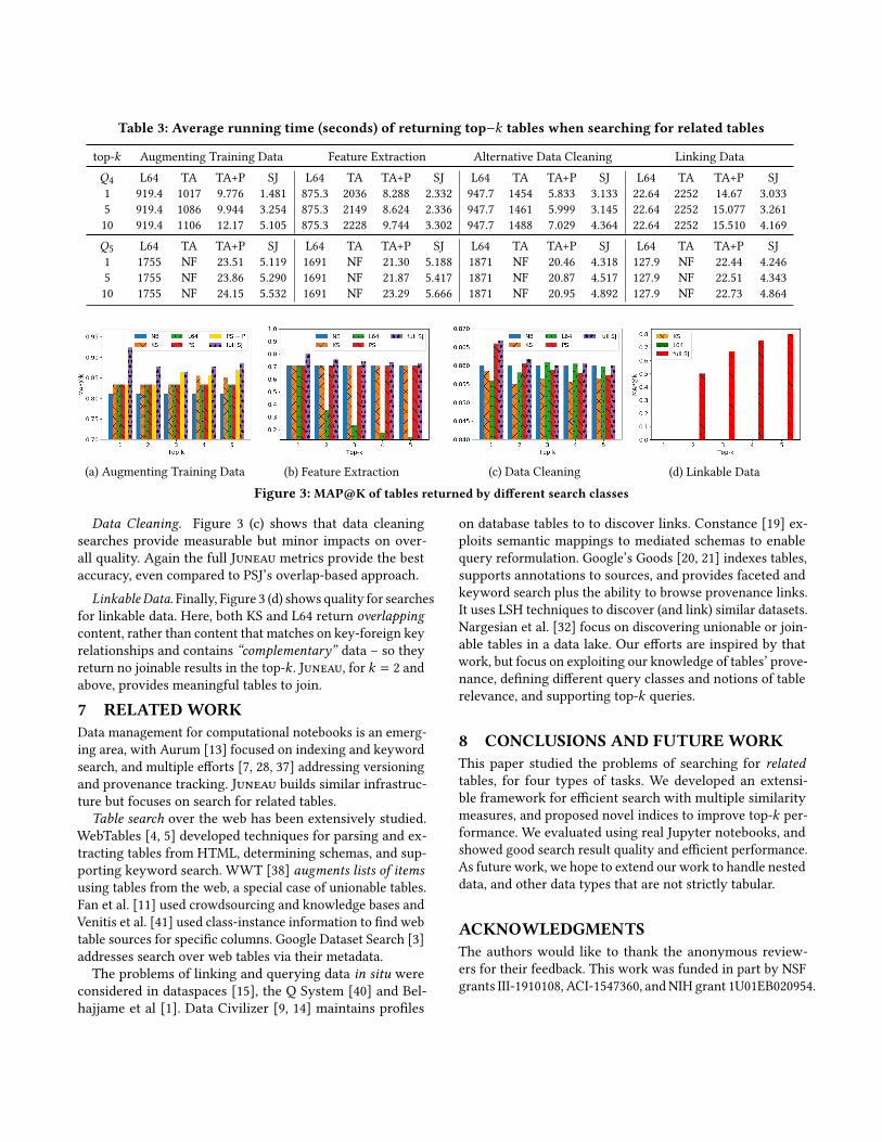
Table 3: Average running time (seconds) of returning top−k tables when searching for related tables

top-k Augmenting Training Data Feature Extraction Alternative Data Cleaning Linking DataQ4 L64 TA TA+P SJ L64 TA TA+P SJ L64 TA TA+P SJ L64 TA TA+P SJ1 919.4 1017 9.776 1.481 875.3 2036 8.288 2.332 947.7 1454 5.833 3.133 22.64 2252 14.67 3.0335 919.4 1086 9.944 3.254 875.3 2149 8.624 2.336 947.7 1461 5.999 3.145 22.64 2252 15.077 3.26110 919.4 1106 12.17 5.105 875.3 2228 9.744 3.302 947.7 1488 7.029 4.364 22.64 2252 15.510 4.169Q5 L64 TA TA+P SJ L64 TA TA+P SJ L64 TA TA+P SJ L64 TA TA+P SJ1 1755 NF 23.51 5.119 1691 NF 21.30 5.188 1871 NF 20.46 4.318 127.9 NF 22.44 4.2465 1755 NF 23.86 5.290 1691 NF 21.87 5.417 1871 NF 20.87 4.517 127.9 NF 22.51 4.34310 1755 NF 24.15 5.532 1691 NF 23.29 5.666 1871 NF 20.95 4.892 127.9 NF 22.73 4.864

(a) Augmenting Training Data (b) Feature Extraction (c) Data Cleaning (d) Linkable Data

Figure 3: MAP@K of tables returned by different search classes

Data Cleaning. Figure 3 (c) shows that data cleaningsearches provide measurable but minor impacts on over-all quality. Again the full Juneau metrics provide the bestaccuracy, even compared to PSJ’s overlap-based approach.

Linkable Data. Finally, Figure 3 (d) shows quality for searchesfor linkable data. Here, both KS and L64 return overlappingcontent, rather than content that matches on key-foreign keyrelationships and contains “complementary” data – so theyreturn no joinable results in the top-k . Juneau, for k = 2 andabove, provides meaningful tables to join.

7 RELATEDWORK

Data management for computational notebooks is an emerg-ing area, with Aurum [13] focused on indexing and keywordsearch, and multiple efforts [7, 28, 37] addressing versioningand provenance tracking. Juneau builds similar infrastruc-ture but focuses on search for related tables.Table search over the web has been extensively studied.

WebTables [4, 5] developed techniques for parsing and ex-tracting tables from HTML, determining schemas, and sup-porting keyword search. WWT [38] augments lists of itemsusing tables from the web, a special case of unionable tables.Fan et al. [11] used crowdsourcing and knowledge bases andVenitis et al. [41] used class-instance information to find webtable sources for specific columns. Google Dataset Search [3]addresses search over web tables via their metadata.The problems of linking and querying data in situ were

considered in dataspaces [15], the Q System [40] and Bel-hajjame et al [1]. Data Civilizer [9, 14] maintains profiles

on database tables to to discover links. Constance [19] ex-ploits semantic mappings to mediated schemas to enablequery reformulation. Google’s Goods [20, 21] indexes tables,supports annotations to sources, and provides faceted andkeyword search plus the ability to browse provenance links.It uses LSH techniques to discover (and link) similar datasets.Nargesian et al. [32] focus on discovering unionable or join-able tables in a data lake. Our efforts are inspired by thatwork, but focus on exploiting our knowledge of tables’ prove-nance, defining different query classes and notions of tablerelevance, and supporting top-k queries.

8 CONCLUSIONS AND FUTUREWORK

This paper studied the problems of searching for relatedtables, for four types of tasks. We developed an extensi-ble framework for efficient search with multiple similaritymeasures, and proposed novel indices to improve top-k per-formance. We evaluated using real Jupyter notebooks, andshowed good search result quality and efficient performance.As future work, we hope to extend our work to handle nesteddata, and other data types that are not strictly tabular.

ACKNOWLEDGMENTS

The authors would like to thank the anonymous review-ers for their feedback. This work was funded in part by NSFgrants III-1910108, ACI-1547360, andNIH grant 1U01EB020954.

REFERENCES

[1] Khalid Belhajjame, Norman W Paton, Alvaro AA Fernandes, CorneliaHedeler, and Suzanne M Embury. 2011. User Feedback as a First ClassCitizen in Information Integration Systems.. In CIDR. 175–183.

[2] William J. Bolosky, John R. Douceur, David Ely, and Marvin Theimer.2000. Feasibility of a Serverless Distributed File System Deployed onan Existing Set of Desktop PCs. In Proc. Measurement and Modeling ofComputer Systems, 2000. 34–43.

[3] Dan Brickley, Matthew Burgess, and Natasha Noy. 2019. GoogleDataset Search: Building a search engine for datasets in an open Webecosystem. In The World Wide Web Conference. 1365–1375.

[4] Michael Cafarella, Alon Halevy, Hongrae Lee, Jayant Madhavan, CongYu, Daisy Zhe Wang, and Eugene Wu. 2018. Ten years of Webtables.Proceedings of the VLDB Endowment 11, 12 (2018), 2140–2149.

[5] Michael J. Cafarella, Alon Y. Halevy, Daisy Zhe Wang, Eugene Wu,and Yang Zhang. 2008. WebTables: exploring the power of tables onthe web. PVLDB 1, 1 (2008), 538–549.

[6] Loredana Caruccio, Vincenzo Deufemia, and Giuseppe Polese. 2016.Relaxed functional dependencies — a survey of approaches. IEEETransactions on Knowledge and Data Engineering 28, 1 (2016), 147–165.

[7] Lucas AMC Carvalho, Regina Wang, Yolanda Gil, and Daniel Garijo.2017. NiW: Converting Notebooks intoWorkflows to Capture Dataflowand Provenance. In Proceedings of Workshops and Tutorials of the 9thInternational Conference on Knowledge Capture (K-CAP2017).

[8] James Cheney, Laura Chiticariu, and Wang Chiew Tan. 2009. Prove-nance in Databases: Why, How, and Where. Foundations and Trendsin Databases 1, 4 (2009), 379–474.

[9] Dong Deng, Raul Castro Fernandez, Ziawasch Abedjan, Sibo Wang,Michael Stonebraker, Ahmed K Elmagarmid, Ihab F Ilyas, SamuelMadden, Mourad Ouzzani, and Nan Tang. 2017. The Data CivilizerSystem.. In CIDR.

[10] Ronald Fagin, Amnon Lotem, and Moni Naor. 2003. Optimal aggre-gation algorithms for middleware. J. Comput. System Sci. 66(4) (June2003), 614–656.

[11] Ju Fan, Meiyu Lu, Beng Chin Ooi, Wang-Chiew Tan, andMeihui Zhang.2014. A hybrid machine-crowdsourcing system for matching webtables. In 2014 IEEE 30th International Conference on Data Engineering.IEEE, 976–987.

[12] Wenfei Fan, Floris Geerts, Jianzhong Li, and Ming Xiong. 2011. Dis-covering conditional functional dependencies. IEEE Transactions onKnowledge and Data Engineering 23, 5 (2011), 683–698.

[13] Raul Castro Fernandez, Ziawasch Abedjan, Famien Koko, Gina Yuan,Samuel Madden, and Michael Stonebraker. 2018. Aurum: A data dis-covery system. In 2018 IEEE 34th International Conference on DataEngineering (ICDE). IEEE, 1001–1012.

[14] Raul Castro Fernandez, Jisoo Min, Demitri Nava, and Samuel Madden.2019. Lazo: A Cardinality-Based Method for Coupled Estimation ofJaccard Similarity and Containment. In 2019 IEEE 35th InternationalConference on Data Engineering (ICDE). IEEE, 1190–1201.

[15] Michael Franklin, Alon Halevy, and David Maier. 2005. From databasesto dataspaces: a new abstraction for information management. SIG-MOD Rec. 34, 4 (2005), 27–33.

[16] Avigdor Gal. 2011. Uncertain Schema Matching. Morgan and Claypool.[17] Timnit Gebru, Jamie Morgenstern, Briana Vecchione, Jennifer Wort-

man Vaughan, Hanna Wallach, Hal Daumeé III, and Kate Crawford.2018. Datasheets for datasets. arXiv preprint arXiv:1803.09010 (2018).

[18] Jeremy Goecks, Anton Nekrutenko, and James Taylor. 2010. Galaxy:a comprehensive approach for supporting accessible, reproducible,and transparent computational research in the life sciences. Genomebiology 11, 8 (2010), R86.

[19] Rihan Hai, Sandra Geisler, and Christoph Quix. 2016. Constance: AnIntelligent Data Lake System. In SIGMOD. ACM, New York, NY, USA,2097–2100. https://doi.org/10.1145/2882903.2899389

[20] Alon Halevy, Flip Korn, Natalya F Noy, Christopher Olston, NeoklisPolyzotis, Sudip Roy, and Steven Euijong Whang. 2016. Goods: Or-ganizing Google’s datasets. In Proceedings of the 2016 InternationalConference on Management of Data. ACM, 795–806.

[21] Alon Y Halevy, Flip Korn, Natalya Fridman Noy, Christopher Olston,Neoklis Polyzotis, Sudip Roy, and Steven Euijong Whang. 2016. Man-aging Google’s data lake: an overview of the Goods system. IEEE DataEng. Bull. 39, 3 (2016), 5–14.

[22] Yka Huhtala, Juha Kärkkäinen, Pasi Porkka, and Hannu Toivonen.1999. TANE: An efficient algorithm for discovering functional andapproximate dependencies. The computer journal 42, 2 (1999), 100–111.

[23] Ihab F. Ilyas, Walid G. Aref, and Ahmed K. Elmagarmid. 2003. Support-ing Top-k Join Queries in Relational Databases. In VLDB. 754–765.

[24] Ihab F Ilyas, Volker Markl, Peter Haas, Paul Brown, and Ashraf Aboul-naga. 2004. CORDS: automatic discovery of correlations and softfunctional dependencies. In Proceedings of the 2004 ACM SIGMODinternational conference on Management of data. ACM, 647–658.

[25] Ihab F. Ilyas and Mohamed Soliman. 2011. Probabilistic Ranking Tech-niques in Relational Databases. Morgan and Claypool.

[26] Jaewook Kim, Yun Peng, Nenad Ivezik, Junho Shin, et al. 2010.Semantic-based Optimal XML Schema Matching: A MathematicalProgramming Approach. In The Proceedings of International Conferenceon E-business, Management and Economics.

[27] Pradap Konda, Sanjib Das, AnHai Doan, Adel Ardalan, Jeffrey R Ballard,Han Li, Fatemah Panahi, Haojun Zhang, Jeff Naughton, Shishir Prasad,et al. 2016. Magellan: toward building entity matching managementsystems over data science stacks. Proceedings of the VLDB Endowment9, 13 (2016), 1581–1584.

[28] David Koop and Jay Patel. 2017. Dataflow notebooks: encoding andtracking dependencies of cells. In 9th USENIX Workshop on the Theoryand Practice of Provenance (TaPP 17). USENIX Association.

[29] Arun Kumar, Jeffrey Naughton, Jignesh M. Patel, and Xiaojin Zhu.2016. To Join or Not to Join? Thinking Twice about Joins beforeFeature Selection. In Proceedings of the 2016 International Conferenceon Management of Data. Association for Computing Machinery, NewYork, NY, USA, 19âĂŞ34. https://doi.org/10.1145/2882903.2882952

[30] Chengkai Li, Kevin Chen-Chuan Chang, Ihab F. Ilyas, and Sumin Song.2005. RankSQL: Query Algebra and Optimization for Relational Top-kQueries. In SIGMOD. 131–142.

[31] Bertram Ludäscher, Ilkay Altintas, Chad Berkley, Dan Higgins, EfratJaeger, Matthew Jones, Edward A. Lee, Jing Tao, and Yang Zhao. 2006.Scientific workflow management and the Kepler system. Concurrencyand Computation: Practice and Experience (2006), 1039–1065.

[32] Fatemeh Nargesian, Erkang Zhu, Renée J Miller, Ken Q Pu, and Patri-cia C Arocena. 2019. Data Lake Management: Challenges and Oppor-tunities. Proceedings of the VLDB Endowment 12, 12 (2019).

[33] Fatemeh Nargesian, Erkang Zhu, Ken Q Pu, and Renée J Miller. 2018.Table union search on open data. Proceedings of the VLDB Endowment11, 7 (2018), 813–825.

[34] T. Oinn, M. Greenwood, M. Addis, N. Alpdemir, J. Ferris, K. Glover,C. Goble, A. Goderis, D. Hull, D. Marvin, P. Li, P. Lord, M. Pocock, M.Senger, R. Stevens, A. Wipat, and C. Wroe. 2006. Taverna: lessons increating a workflow environment for the life sciences. Concurrencyand Computation: Practice and Experience 18, 10 (2006), 1067–1100.

[35] Christos H Papadimitriou. 1981. On the complexity of integer pro-gramming. Journal of the ACM (JACM) 28, 4 (1981), 765–768.

[36] Fernando Perez and Brian E Granger. 2015. Project Jupyter: Computa-tional narratives as the engine of collaborative data science. RetrievedSeptember 11 (2015), 207.

[37] Tomas Petricek, James Geddes, and Charles Sutton. 2018. Wrattler:Reproducible, live and polyglot notebooks. In 10th USENIXWorkshop onthe Theory and Practice of Provenance (TaPP 2018). USENIXAssociation.

[38] Rakesh Pimplikar and Sunita Sarawagi. 2012. Answering Table Querieson the Web using Column Keywords. PVLDB 5, 10 (2012), 908–919.

[39] Erhard Rahm and Philip A. Bernstein. 2001. A Survey of Approachesto Automatic Schema Matching. VLDB J. 10, 4 (2001), 334–350.

[40] Partha Pratim Talukdar, Marie Jacob, Muhammad Salman Mehmood,Koby Crammer, Zachary G. Ives, Fernando Pereira, and Sudipto Guha.2008. Learning to create data-integrating queries. PVLDB 1, 1 (2008),785–796.

[41] Petros Venetis, Alon YHalevy, JayantMadhavan,Marius Pasca,WarrenShen, Fei Wu, and Gengxin Miao. 2011. Recovering semantics of tableson the web. (2011).

[42] Daisy ZheWang, Xin Luna Dong, Anish Das Sarma, Michael J Franklin,and Alon Y Halevy. 2009. Functional Dependency Generation andApplications in Pay-As-You-Go Data Integration Systems. In WebDB.

[43] Zhiping Zeng, Anthony KH Tung, Jianyong Wang, Jianhua Feng, andLizhu Zhou. 2009. Comparing stars: On approximating graph editdistance. Proceedings of the VLDB Endowment 2, 1 (2009), 25–36.

[44] Yi Zhang and Zachary G. Ives. 2019. Juneau: Data Lake Managementfor Jupyter. Proceedings of the VLDB Endowment 12, 7 (2019).

[45] Erkang Zhu, Dong Deng, Fatemeh Nargesian, and Renée J Miller. 2019.JOSIE: Overlap Set Similarity Search for Finding Joinable Tables inData Lakes. In Proceedings of the 2019 International Conference onManagement of Data. ACM, 847–864.

[46] Erkang Zhu, Fatemeh Nargesian, Ken Q Pu, and Renée J Miller. 2016.LSH ensemble: internet-scale domain search. Proceedings of the VLDBEndowment 9, 12 (2016), 1185–1196.

[47] Moshé M. Zloof. 1975. Query-by-example: the invocation and defini-tion of tables and forms. In VLDB ’75: Proceedings of the 1st InternationalConference on Very Large Data Bases. 1–24.

[48] Moshé M. Zloof. 1977. Query By Example: A Data Base Language.IBM Systems Journal 16(4) (1977), 324–343.