finding paraphrases using pnrule - …ftp.cs.toronto.edu/pub/gh/bartlett-thesis.pdf · abstract...
TRANSCRIPT

FINDING PARAPHRASES USING PNRULE
by
Benjamin Bartlett
A thesis submitted in conformity with the requirementsfor the degree of Master of Science
Graduate Department of Computer ScienceUniversity of Toronto
Copyright c�
2006 by Benjamin Bartlett

Abstract
Finding Paraphrases Using PNrule
Benjamin Bartlett
Master of Science
Graduate Department of Computer Science
University of Toronto
2006
In this thesis, we attempt to use a machine-learning algorithm, PNrule, along with simple
lexical and syntactic measures to detect paraphrases in cases where their existence is rare. We
choose PNrule because it was specifically developed for classification in instances where the
target class is rare compared to other classes within the data. We test our system both on a
dataset we develop based on movie reviews, and on the PASCAL RTE dataset; we obtain poor
results on the former, and moderately good results on the latter. We examine why this is the
case, and suggest improvements for future research.
ii

Acknowledgements
I’d like to thank my supervisor, Graeme Hirst, my second reader, Gerald Penn, my two anno-
tators, Paul and Tim, the Natural Sciences and Engineering Research Council of Canada, and,
of course, my family.
iii

Contents
1 Introduction 1
2 Background 2
2.1 Paraphrases . . . . . . . . . . . . . . . . . . . . . . . . . . . . . . . . . . . . 2
2.2 Why use machine learning to detect paraphrases? . . . . . . . . . . . . . . . . 2
2.3 Machine learning and rare classes . . . . . . . . . . . . . . . . . . . . . . . . 4
2.3.1 What is a rare class? . . . . . . . . . . . . . . . . . . . . . . . . . . . 4
2.3.2 What makes learning rare classes difficult? . . . . . . . . . . . . . . . 5
2.4 Rule-based machine learning . . . . . . . . . . . . . . . . . . . . . . . . . . . 6
2.4.1 Why rule-based? . . . . . . . . . . . . . . . . . . . . . . . . . . . . . 6
2.4.2 Methods for rule-based machine learning . . . . . . . . . . . . . . . . 7
2.5 PNrule . . . . . . . . . . . . . . . . . . . . . . . . . . . . . . . . . . . . . . . 19
2.5.1 Two-phase rule induction . . . . . . . . . . . . . . . . . . . . . . . . . 19
2.5.2 Scoring mechanism . . . . . . . . . . . . . . . . . . . . . . . . . . . . 27
3 Related Work 34
3.1 Shinyama, Sekine, and Sudo 2002 . . . . . . . . . . . . . . . . . . . . . . . . 34
3.2 Barzilay and Lee 2003 . . . . . . . . . . . . . . . . . . . . . . . . . . . . . . 39
3.3 Barzilay and Elhadad 2003 . . . . . . . . . . . . . . . . . . . . . . . . . . . . 43
3.4 Quirk, Brockett, and Dolan 2004 . . . . . . . . . . . . . . . . . . . . . . . . . 48
3.5 The PASCAL Recognizing Textual Entailment Challenge . . . . . . . . . . . . 53
iv

3.5.1 The challenge . . . . . . . . . . . . . . . . . . . . . . . . . . . . . . . 53
3.5.2 The systems . . . . . . . . . . . . . . . . . . . . . . . . . . . . . . . . 56
3.5.3 Discussion of results . . . . . . . . . . . . . . . . . . . . . . . . . . . 65
3.6 What makes our method different? . . . . . . . . . . . . . . . . . . . . . . . . 67
4 Finding Paraphrases Using PNrule 68
4.1 Our goal . . . . . . . . . . . . . . . . . . . . . . . . . . . . . . . . . . . . . . 68
4.2 Our corpus . . . . . . . . . . . . . . . . . . . . . . . . . . . . . . . . . . . . 69
4.3 Measuring the signature clarity of a model . . . . . . . . . . . . . . . . . . . . 71
4.4 Changes to PNrule . . . . . . . . . . . . . . . . . . . . . . . . . . . . . . . . 73
4.5 Preprocessing . . . . . . . . . . . . . . . . . . . . . . . . . . . . . . . . . . . 74
4.5.1 Expanding contractions . . . . . . . . . . . . . . . . . . . . . . . . . . 75
4.5.2 Part-of-speech tagging . . . . . . . . . . . . . . . . . . . . . . . . . . 75
4.5.3 Removing extra verbs . . . . . . . . . . . . . . . . . . . . . . . . . . 75
4.5.4 Removing certain parts of speech . . . . . . . . . . . . . . . . . . . . 76
4.6 Measures . . . . . . . . . . . . . . . . . . . . . . . . . . . . . . . . . . . . . 76
4.6.1 Regularization of continuous measures . . . . . . . . . . . . . . . . . 77
4.6.2 Word-stem matching . . . . . . . . . . . . . . . . . . . . . . . . . . . 78
4.6.3 Using WordNet . . . . . . . . . . . . . . . . . . . . . . . . . . . . . . 79
4.6.4 Using VerbNet . . . . . . . . . . . . . . . . . . . . . . . . . . . . . . 80
4.6.5 Bigram and trigram matching . . . . . . . . . . . . . . . . . . . . . . 81
4.6.6 Skip-one bigram matching . . . . . . . . . . . . . . . . . . . . . . . . 81
4.6.7 Matching within a window . . . . . . . . . . . . . . . . . . . . . . . . 82
4.6.8 Latent semantic indexing . . . . . . . . . . . . . . . . . . . . . . . . . 83
4.6.9 Using the similarity of containing paragraphs . . . . . . . . . . . . . . 83
4.6.10 Complex measures . . . . . . . . . . . . . . . . . . . . . . . . . . . . 84
4.6.11 Matching words with different parts of speech . . . . . . . . . . . . . . 85
4.7 Results . . . . . . . . . . . . . . . . . . . . . . . . . . . . . . . . . . . . . . . 86
v

4.8 Results on RTE dataset . . . . . . . . . . . . . . . . . . . . . . . . . . . . . . 89
4.9 Analysis . . . . . . . . . . . . . . . . . . . . . . . . . . . . . . . . . . . . . . 91
5 Future Work 96
5.1 Preprocessing . . . . . . . . . . . . . . . . . . . . . . . . . . . . . . . . . . . 96
5.2 Method . . . . . . . . . . . . . . . . . . . . . . . . . . . . . . . . . . . . . . 97
5.3 Machine Learning . . . . . . . . . . . . . . . . . . . . . . . . . . . . . . . . . 97
5.4 Measures . . . . . . . . . . . . . . . . . . . . . . . . . . . . . . . . . . . . . 98
Bibliography 100
vi

Chapter 1
Introduction
Merriam-Webster’s dictionary defines a paraphrase as ”a restatement of a text, passage, or work
giving the meaning in another form.” Recently, there has been a lot of work in computational
linguistics towards developing systems that can automatically detect paraphrases. There are
a number of ways in which such a system could be useful; some examples include: as part
of an automatic summarization system, removing multiple instances of the same information;
looking for the recurrence of an idea within a particular body of work; detecting political
talking points in a body of news articles; or creating a dataset that can be used by a system that
automatically learns how to generate paraphrases, in the same way that aligned sentences are
used in systems that learn how to translate between two languages.
Most of the work up to this point has dealt primarily with paraphrases that occur within
parallel corpora—situations in which paraphrases occur relatively frequently, and are often
lexically similar to the text unit they paraphrase. While this has led to useful systems, we feel
the next obvious step is to attempt to detect paraphrases in situations where they occur rarely,
and are not necessarily lexically similar to the text unit they paraphrase. In this thesis, we
attempt to do just that, using a machine learning technique in combination with a set of simple
lexical and syntactic measures.
1

Chapter 2
Background
2.1 Paraphrases
Given two texts, T and P, we say that P is a paraphrase of T if the semantic meaning of P is
found entirely in T , with the possible aid of world knowledge (e.g., that a German shepherd is
a breed of dog). Some loss of information is acceptable; for instance, “A dog went to the store.”
is an acceptable paraphrase of “A German shepherd ran to the store.” The latter is more specific
than the former—we know the breed of the dog, and have some sense of the rate at which it
traveled—but both convey the same basic meaning. However, in a case where information
loss occurs, the paraphrase relationship is asymmetric; it would not be accurate to state that “A
German shepherd ran to the store.” is a paraphrase of “A dog went to the store.”
2.2 Why use machine learning to detect paraphrases?
There are several reasons to use machine learning to detect paraphrases. First, there’s the fact
that machine-learning approaches have been used successfully to solve many other natural-
language-processing problems. Marquez (2000) lists many of these problems, including: sense
discrimination, word sense disambiguation, text classification, speech recognition, part-of-
speech tagging, text summarization, dialog act tagging, co-reference resolution, cue phrase
2

CHAPTER 2. BACKGROUND 3
a. An OH-58 helicopter, carrying a crew of two, was on a routine training orientation
when contact was lost at about 11:30 a.m. Saturday (9:30 p.m. EST Friday).
b. “There were two people on board,” said Bacon. “We lost radar contact with the
helicopter about 9:15 EST (0215 GMT).”
Figure 2.1: Example of two text units that are similar, but where neither is a paraphrase of the
other. From Hatzivassliloglou et al. (1999).
identification, machine translation, homograph disambiguation in speech synthesis, accent
restoration, PP-attachment disambiguation, phonology, morphology, and spelling correction.
Second, and more importantly, machine learning has been used, with some success, to solve
a very similar problem: Hatzivassliloglou et al. (1999) use it to match similar pairs of small
textual units (in particular, paragraphs, although in theory their technique could be applied
to sentences as well). They consider two textual units to be similar if they share the same
focus on a common concept, actor, object, or action, and if that common actor or concept
either performs or is the subject of the same action. This definition includes paraphrases, but
it includes other sorts of relationships as well. Hatzivassliloglou et al. (1999) focused on news
stories about the same event, in which such similar text units are likely to arise; we’re hoping
to detect paraphrases in corpora where they are much less likely to arise.
So far we have shown that a machine-learning approach could potentially be used to solve
the problem of classifying paraphrases. But we still have not explained why it should be used.
Our reasoning is basically this: while ideally, we’d like to simply look at the semantics of
two textual units (in our case, clauses) and decide whether or not they are the same; however,
building semantical forms of sentences and rules that encode world knowledge is very difficult.
Instead, we rely on syntactic and lexical clues to decide whether or not one textual unit is a
paraphrase of another. While some clues may be the same across the English language, others

CHAPTER 2. BACKGROUND 4
likely vary depending upon the corpus, both due to different styles of writing, and due to
different contexts. In addition, even if a clue does exist across the entire language, it may
be more important within some corpora than within others. Because we don’t believe that it
is currently possible to develop a system that can, out of the box, detect paraphrases in any
corpus, we feel that it is best to develop a system that can be easily trained to deal with a new
situation.
This leads us to our final point: simplicity. Machine-learning algorithms are much easier to
adapt to new situations than are finely-tailored solutions. While the latter may be preferable in
some cases, what we’d like to see is a machine-learning algorithm combined with a toolbox of
syntactic and lexical features which could easily be trained on new corpora. This has the added
benefit of allowing people to easily add new features to the toolbox (there are any number of
features we have not tried yet, some of which could prove quite useful). There is, of course,
one weakness to our approach: because it’s a supervised method, we need annotated corpora,
the production of which can be quite time consuming. This could potentially be overcome
using an unsupervised approach, however because such an approach would require us to de-
vise a heuristic to generate examples, we were concerned that the resulting model would not
accurately reflect human judgment about paraphrases. A supervised method would avoid this
problem.1
2.3 Machine learning and rare classes
2.3.1 What is a rare class?
A class is rare when the number of examples of that class is proportionally very small compared
to the number of examples of other classes in the training and testing data. While it is difficult
to quantify this precisely, Joshi (2002) states that, while it’s possible for a class covering up
1However, an unsupervised method may well be worth researching in the future.

CHAPTER 2. BACKGROUND 5
to 35% of a training set to be considered rare, a rare class is generally one that covers at most
10% of the training examples. Unless we are considering two highly similar corpora, it’s likely
that paraphrases will be a rare class under this definition.
As we are concerned only with binary classification—either a pair of sentences contains
clauses that are paraphrases of one another, or they do not—for further discussion, borrowing
from Joshi (2002), we will use C to refer to the rare class, and NC to refer to its complement.
2.3.2 What makes learning rare classes difficult?
Joshi (2002) lists three issues that arise in the context of a rare class that make learning difficult
(note that we have simply borrowed Joshi’s terms for these problems):
Low Separability Occasionally, one encounters a case where the data are noise-free and the
examples can be classified using only one or two attributes. In this case, the data have
a high degree of separability, and only a very simple classification model is needed.
Usually, however, the records of class C are distributed in small clusters throughout
various subspaces of the attribute space. This makes it difficult to find a large cluster
containing records of class C that does not also contain a number of examples of class
NC. This low degree of separability makes classification more difficult, and thus a more
complicated model is required.
Multi-modality of the classes Related to separability is the fact that C and, in particular, NC
may consist of different subclasses with different characteristics. It may be easy to sep-
arate C from some of those subclasses, but very difficult to separate it from others. We
will see an example of this later in the chapter.
Rarity The rarity of the class is itself a problem. In particular, it’s very difficult to avoid over-
fitting the model to C: since the set of records in C is so much smaller than the set of
records in NC, it’s easy to find a model that fits those few positive examples exactly, but

CHAPTER 2. BACKGROUND 6
then doesn’t generalize well. Thus, it performs well on the training data, but not on the
testing data.
2.4 Rule-based machine learning
One set of commonly-used methods in machine learning falls into a group that we will call
“rule-based machine learning”. Given as data a set of records made up of attribute-value pairs,
a rule is a set of conditions that a record must meet in order to be placed into a particular class.
Each rule can thus be described as a conjunction within propositional logic (Mitchell, 1997).2
Ideally, then, the model would consist of a single rule for each class. However, recall that we
earlier mentioned the multi-modality of the classes. This means that it’s likely that each class
will be made up of subclasses, each with its own signature—that is, its own set of values that
indicate its existence. In order to handle this, the model must instead be a set of rules; if a
record satisfies any single rule that indicates it belongs to a particular class, it is placed into
that class. It is those machine-learning approaches that build as their models disjunctions of
rules that we are referring to as rule-based machine-learning algorithms.
2.4.1 Why rule-based?
The main reason we feel that rule-based machine learning should be used for this task is that, as
mentioned by Mitchell (1997) and Joshi (2002), a rule-based method is easily interpretable by
humans. We believe this to be particularly important in the domain of paraphrase identification.
Human beings have some intuition as to what attributes are likely to indicate the occurrence of
paraphrases. Using a rule-based approach, they can see how well their intuition fits with what’s
discovered by the machine learning algorithm. This is advantageous for several reasons: first,
we are more likely to catch errors in the software we use to obtain the attribute-value pairs, since
such errors will cause situations where the results do not match our expectations. For example,
2There are also methods for learning first-order logic models, but we are not concerned with these.

CHAPTER 2. BACKGROUND 7
if we find that the presence of matching trigrams between two sentences indicates that they are
not paraphrases of one another, we know that we should take a second look at our trigram-
matching algorithm. Second, in the case where the differences are not caused by an error, we
may learn something new about the problem. Finally, because we can associate a record with
the rule that classified it, we can look at false positives and discover both what attributes are
indicating that these examples are positive, and, by looking at the sentences themselves, what
additional attributes might allow us to distinguish between false and true positives. These are
opportunities that less easily understood classification methods might not afford us.
A second reason for focusing on rule-based machine learning is that, compared to some
other approaches, the parameters to the algorithm are relatively intuitive. One has a sense of
what it means to have an upper bound on the length of a rule, or a lower bound on its accuracy.
Compare this with, for example, support vector machines, where one has to decide between
using a radial or an exponential kernel space. It’s much more difficult to understand what the
latter “means” in terms of the problem one is trying to solve.
2.4.2 Methods for rule-based machine learning
While there are a number of methods for building rule-based models, the two most common
are to build a decision tree, in which case each path through the tree can be considered a rule3,
or to attempt to discover the rules directly (Mitchell, 1997). We will refer to the former as the
“decision-tree-construction” method or approach, and the latter as the “rule-induction” method
or approach. We will describe both of these approaches, will explain why a rule-induction
approach is better suited to cases in which the target class is rare, and will then explain where
the rule-induction approach falls short in such cases.
3C4.5rules actually explicitly transforms the tree into rules, with consequences that will be described later.Any decision tree can be viewed as a conjunction of disjunctive rules, however.

CHAPTER 2. BACKGROUND 8
Figure 2.2: An example of a decision tree, for the class IS-AN-APPLE.
Decision-tree-construction methods
In order to understand decision-tree-construction methods, it is first helpful to understand how
a decision tree is used to classify a record. A decision tree is made up of leaf nodes, each of
which has a class associated with it, and inner or decision nodes, each of which has an attribute
associated with it. There are branches from each decision node corresponding to the possible
values of its associated attribute. In order to classify a record, one simply starts at the root node,
and for each attribute picks the path that corresponds to the value of that attribute in the record,
until one reaches a leaf node. The record is labeled with the class associated with the leaf node.
Note that an attribute may only appear once in a given path; to appear more than once would
simply be redundant, as the attribute value for the record has already been determined.4
An example of a decision tree can be seen in Figure 2.2. This tree tries to determine whether
a fruit is an apple by means of three attributes: color, peel, and shape. Color can take on the
value yellow, red, or green; peel can take on the value thick or thin; and shape can take on
4One reader brought up the question of whether this would be true if the tree were required to be binary. Theanswer is a qualified yes: each attribute would have to be replaced with a set of attributes that took binary values,and each of these new attributes could only appear once in each path.

CHAPTER 2. BACKGROUND 9
the value round or football. Each path through the tree is distinguished by the values these
attributes take on; the final node in the path describes whether the fruit is in the target class or
not. This is, of course, a fairly silly example, but nevertheless, demonstrates how a decision
tree works.
There are a number of efficient decision-tree-construction algorithms, but they are all vari-
ations of an algorithm that does a top-down greedy search through the hypothesis space of
all possible decision trees. Mitchell (1997), from whom we draw much of this information,
states that the two algorithms that most exemplify this approach are ID3 (Quinlan, 1986) and
its descendant, C4.5 (Quinlan, 1993). Certainly the latter is one of the most, if not the most
widely-used decision-tree-construction algorithms. In general, the algorithm operates as fol-
lows, beginning at the root node of a single-node tree: The algorithm must use some fitness
measure, such as information gain or gain ratio5, to decide what attribute best separates the
instances by class. This attribute is then used as the test for the current node, a branch is created
for each possible value of that attribute, and at the end of each branch a new leaf node is cre-
ated. The process is then repeated for each of these descendant nodes, using only those training
examples covered by the attribute value associated with the branch leading to the descendant
node and only those attributes not already selected. This continues until each potential path
through the tree either has only one class associated with it, or has every possible attribute in
it.
One thing to note is that the algorithm, as described so far, works only if the attributes can
only take on discrete values. However, it is possible for decision-tree-construction methods
to handle continuous attributes. The idea is that instead of using the values of the attribute
directly, the algorithm creates a new attribute Ac, which for each record has as its value the
truth value of A � c, where A is the continuous attribute, and c is some threshold. To find this
threshold, the algorithm sorts the training examples by the values of A. Then, the algorithm
iteratively sets c to the halfway point between two adjacent examples, and tests this threshold
5We won’t describe these measures here, as we don’t use them in our method.

CHAPTER 2. BACKGROUND 10
using information gain. Whichever c scores highest is used as the threshold (Mitchell, 1997).
One serious weakness of this approach is that it is prone to over-fitting. Two approaches
have been taken to combat this problem:
1. stopping the growth of the tree before it over-fits; or
2. allowing the tree to over-fit, and then pruning it.
The latter of the two approaches has been shown to be more effective (Mitchell, 1997), so we
will examine it further.
One possible implementation of this approach, called reduced-error pruning (Quinlan,
1987), begins by splitting the training data into a training set and a validation set. For each
decision node, the method creates a pruned tree by removing the subtree rooted at that decision
node, making it a leaf node. It then assigns the most-frequently-appearing class of training
examples covered by the pruned node to that node. For example, if the pruned node covered
5 examples of class A, and 7 examples of class B, then the pruned node would be labeled with
class B. If the pruned tree does no worse than the current tree, it is used; otherwise, the current
tree is kept. At any iteration there could be several possible pruned trees that do no worse than
the current tree; in this case, the method picks the pruned tree that most increases the accuracy
over the validation set. The idea behind this implementation is that while the algorithm may
be fooled by noise in the training set, that same noise is unlikely to be present in the validation
set. As Mitchell (1997) notes, this method works well with large amounts of training data, but
will further reduce already small training sets. As we’re dealing with a very rare class, splitting
the training data might eliminate vital positive examples; it would be too easy to eliminate
a subclass of the target class by removing just a few examples. Thus, we can eliminate this
approach from our consideration.
Another implementation is that used in C4.5 (Quinlan, 1993), called rule post-pruning.
Instead of pruning the decision tree, Quinlan first converts the decision tree into a conjunc-
tion of rules; as we mentioned earlier, any decision-tree model can be represented as such a

CHAPTER 2. BACKGROUND 11
conjunction; however, Quinlan makes this transformation explicit. He does so by creating a
conjunctive rule for every path through the tree. From each rule, he removes any condition
whose removal does not reduce the accuracy of the rule set. As above, if there’s more than
one possible pruning, the one that causes the highest increase in accuracy is chosen. Once the
rules have been pruned, they are sorted by their estimated accuracy, and are then applied in this
order during classification (Mitchell, 1997).
There are two advantages to this pruning method. First, transforming the decision tree into
a conjunction of rules allows the algorithm to take into consideration the context within which
a particular decision node is used. Within one path, a decision node could be vital, whereas
within another path, the same decision node could be utterly irrelevant. Because the paths
are converted into rules, the algorithm can remove the node within the context in which it is
irrelevant, while leaving it in the context in which it is vital. Reduced-error pruning could only
distinguish whether a node was relevant to the tree as a whole, and can only decide to remove
it from all paths that go through it, or from none. Second, by converting the paths to rules,
this method removes the distinction between decisions that occur near the root of the tree, and
those that occur near the leaves of the tree. This has two consequences: while within a tree,
one would almost never remove a node near the root, because it has a large effect on the tree
as a whole, within a rule one might remove such a node, because it may have little or no effect
within the context of that rule; and bookkeeping is made much easier, because one no longer
has to remove all the nodes below a removed node.
Aside from pruning rules instead of the decision tree, another difference between rule post-
pruning and reduced-error pruning is the method by which accuracy is estimated. Instead of
using a validation set, rule post-pruning uses the training data with a pessimistic estimate of
accuracy. It calculates the accuracy of a rule over the training examples, and the standard
deviation of that accuracy, assuming a binomial distribution. It then subtracts the latter from
the former. Because of this, for large data sets, the estimated accuracy will be close to the
observed accuracy; but, for smaller data sets, the estimated accuracy will be further from the

CHAPTER 2. BACKGROUND 12
observed accuracy. Thus, rules that cover only a few positive examples will have a very low
estimated accuracy and are more likely to be pruned. While normally this is precisely the
behavior that you’d want—pruning rules that cover only a few examples with high accuracy in
favor of rules that cover a number of examples with somewhat less accuracy—in a case with
rare classes, any good rule is likely to cover only a few examples with high accuracy. A model
with several low-coverage, high-accuracy rules might be precisely what we’d want in such a
case.
Thus, while rule post-pruning might work, at least in some situations, it seems that we
might be better served by modeling the rule set directly. With that in mind, let’s take a look at
rule induction.
Rule-induction methods
As mentioned previously, both decision-tree-construction methods and rule-induction meth-
ods build models which can be described by a set of conjunctive rules. A decision-tree-
construction method does so by searching the hypothesis space of decision trees. In contrast, a
rule-induction method does so by directly searching the hypothesis space of sets of conjunctive
rules (Mitchell, 1997).
There are two methods for rule induction: specific-to-general, and general-to-specific. The
former isn’t tractable for high-dimension datasets, and so most algorithms use the latter (Agar-
wal and Joshi, 2000). The most common method for general-to-specific rule induction is a
method called sequential covering (Agarwal and Joshi, 2000; Mitchell, 1997), which we will
now describe.
Borrowing from Mitchell (1997), we will first describe a subroutine called LEARN-ONE-
RULE. This subroutine accepts a set of positive and negative training examples, and outputs a
rule that covers many of the positive examples while covering few of the negative examples.
This rule must have high accuracy—most of the examples it covers must be positive—but not
necessarily high coverage—it is allowed to cover only a small number of examples.

CHAPTER 2. BACKGROUND 13
One possible implementation of LEARN-ONE-RULE, again taken from Mitchell (1997), is
as follows: begin with a trivial rule that classifies all examples as positive. At each iteration,
try all of the possible attribute tests, and pick whichever one most improves the performance
measure over the training data. Repeat this until the rule has reached an acceptably high level
of accuracy. Note that this is a greedy general-to-specific search through the space of possible
conjunctive rules. There is no backtracking, so it is possible that a suboptimal choice will be
made during the search. Most rule-induction methods use some variation of this approach.
Sequential covering is the method by which the hypothesis space is searched. It works
as follows: first, the training set is fed into LEARN-ONE-RULE, which returns a single high-
accuracy rule. Next, the examples covered by this rule are removed from the training set, and
the new training set is again fed into LEARN-ONE-RULE. This process is repeated until the
model has achieved a satisfactory overall accuracy, or until there remain no positive examples
not covered by an existing rule. This is one of the most widespread approaches to learning a
set of rules (Mitchell, 1997).
So why is a rule-induction approach superior to a decision-tree-construction approach? One
might expect, given Mitchell’s statement that decision trees may be more effective when data is
scarce, that a decision-tree-construction method would be a better approach. However, as Joshi
(2002) points out, a decision-tree-construction method is evaluated by how well it separates
the two classes, the target class and the non-target class. This is fine if the signature for the
target class is very pure, but this is often not the case for rare classes. Rule-induction methods,
on the other hand, are able to simply focus in on the target class. This gives us the ability to
control the recall and precision of the algorithm in a way that is not possible with decision-
tree-construction approaches. This is particularly important in the case of rare classes.
Rare classes are still hard
While sequential covering is a better approach to building a model to classify rare classes
than constructing a decision tree, it is still far from ideal. Joshi (2002) cites two significant

CHAPTER 2. BACKGROUND 14
problems with this approach. The first is a fairly well-known problem called the problem of
small disjuncts (Holte et al., 1989).
A small disjunct is one that correctly classifies only a few training cases. They are much
more error-prone than large disjuncts (Holte et al., 1989). However, they collectively cover
a significant percentage of examples, and thus cannot simply be ignored (Weiss, 1995). This
is particularly true when dealing with rare classes, where even a few missed examples can
lead to a far lower recall for a particular class. Unfortunately, because there are few positive
training examples, a rare class tends to engender small disjuncts—because there aren’t that
many examples to begin with, a rule targeting a rare class probably will correctly classify only
a few training cases, even if it is highly accurate. For example, if there are only 10 records in
class A, out of perhaps a total of 1000 records, a rule R which predicts A and covers 4 of those
examples and no other examples is highly accurate and covers a significant percentage of the
examples of class A, but is still a small disjunct. To make matters worse, sequential covering
removes some of those already-few examples at each iteration (Weiss, 1995; Joshi, 2002).
We should take a moment to distinguish between errors in a model, and errors in a disjunct.
In both cases, an error is a misclassified record. However, while in a model this refers to both
false positives and false negatives, in a disjunct it refers only to false positives. This is because
a disjunct claims only that if a record satisfies it, that record will be in the class it predicts. It
makes no claim about records that do not satisfy it.
Weiss (1995) gives several reasons why small disjuncts are prone to errors:
Bias Inductive bias is the policy by which a machine learning algorithm generalizes beyond
the training examples it is given (Mitchell, 1997). Holte et al. (1989) found that biases
that work well for large disjuncts do not work well for small disjuncts. In particular, the
“maximum generality” bias, which states that an algorithm should find the maximally-
general disjunct that matches a particular set of training examples and no others, works
very poorly for small disjuncts. Holte instead suggests a “selective specificity” bias,
which, after deciding to create a disjunct that matches a set of examples, would then de-

CHAPTER 2. BACKGROUND 15
cide what sort of bias to use to pick between possible disjuncts matching these examples.
Unlike the other four problems, which we mention below, bias is not a problem inherent
to data containing rare classes, but instead is a consequence of using methods designed
to learn models that classify frequently-occurring classes to attempt to learn models that
classify rare classes.
Attribute noise Attribute noise changes the values of the attributes of the records. This can
have different effects, depending on whether it is introduced into the testing set or the
training set. If it is introduced into the testing set, it can cause records to be misclassified.
With rare classes, even a few such misclassifications can have a large effect on the accu-
racy of the model. Worse, if it’s introduced into the training set, it can cause the wrong
model to be learned. This is particularly problematic when dealing with rare classes;
since there are only a small number of examples of a rare class in the first place, even
a few such transformations can cause the target class to be overwhelmed. For example,
imagine there are two classes, M and N, which differ on a single binary attribute: M has
the value 0 for attribute A, and N has the value 1. If the two classes are approximately
the same size, then a bit of attribute noise changes things very little. However, imagine
that examples of class N occur over one hundred times more frequently than examples
of class M. Even if just a small percentage of the N examples have their value for A
transformed into 0 by noise, there could well end up being more N-class examples with
that value than M-class examples. In such a case, a machine learning algorithm would
learn to classify examples with M’s signature as N. Generalization can exacerbate this
problem, since they often work by removing the distinction between two signatures and
then classifying both as whichever class occurs more frequently in the records with the
now-indistinguishable signatures. While we do not have to deal with noise being intro-
duced into our system, the attributes we use are noisy by the nature of our data; thus, this
will be a problem for us.

CHAPTER 2. BACKGROUND 16
Missing attributes When an attribute is missing, two records that would normally be easily
placed into two different classes may instead appear to be the same. If this happens
during testing, the system will have to guess somehow. If it happens during training, the
model will learn to classify such records by whichever class appears more frequently;
in the case where the target class is rare, this likely will be the non-target class. We
encounter this in our latent semantic indexing measure: some of the textual units contain
no indexing terms, and thus cannot be compared to other textual units. We’ll discuss this
further when we describe our experiments.
Class noise Class noise causes a record to be mislabeled. The problems in this situation are
similar to those caused by attribute noise. In our particular case, this could arise if an
annotator missed a paraphrase.
Training set size Weiss (1995) states:
Training set size also has an impact on learning. Rare cases will have a higher
error rate than common cases since they are less likely to be found in the
training set. The small disjuncts will tend to be more error prone because they
cover fewer correct cases than large disjuncts.
We are uncertain as to why Weiss believes this will necessarily cause small disjuncts to
be more error-prone (although one reader suggested bias). However, we’d like to add that
this certainly makes the model containing the small disjuncts more error-prone. Because
small disjuncts cover only a few positive examples, if there are a lot of positive examples
in the population that aren’t in your sample (or if you stop the learning algorithm early,
although this is not a concern in our case), it’s far more likely that there will be positive
examples in the testing set that are not covered by any of the small disjuncts. This leads
to a higher error rate in a model with small disjuncts than in one with large disjuncts.
There could even be positive examples that appear in the testing data that do not have a

CHAPTER 2. BACKGROUND 17
similar signature to anything in the training data, and, because the class is rare, just a few
such examples would lead to a dramatically higher error rate.
The second potential problem is identified by Agarwal and Joshi (2000) and Joshi (2002)
as the problem of splintered positives. This problem arises when the signature for the target
class is a composite of attributes that indicate the presence of the target class, and attributes
that indicate the absence of the non-target class. Since we’re dealing with paraphrases in this
thesis, let us consider an example in that domain: imagine that we have a number of pairs of
sentences, most of which have nothing to do with one another. On the other hand, a few pairs
of sentences will look like this:
a. The elephant sitting on the dock was very large.
b. The elephant sitting on the dock was huge.
It would thus seem that a high lexical similarity between a pair of sentences would be a good
indication of the presence of our target class. However, remember that earlier we mentioned
the multi-modality of classes. Although pairs of unrelated sentences make up a large subclass
of the non-target class, there also could be a subclass that contains pairs of sentences with
opposite meanings. This subclass might contain such pairs as:
a. The horse ran past the barn was very large.
b. The horse ran past the barn was very small.
Like the first pair, this pair would have a very high lexical similarity. However, clearly it is not
a paraphrase. Instead, we need some other attribute, such as the presence of an antonym, to
indicate the presence of the non-target class.
We should emphasize that the problem is not that an algorithm using sequential covering
couldn’t create a model that accounted for the presence of such an attribute; the problem is
with how it would do so. Because of its high accuracy constraints, a sequential covering
approach would refine its current rule, adding another conjunctive condition to it (in the case

CHAPTER 2. BACKGROUND 18
of our example, it might refine the rule “HIGHLEXICALSIMILARITY � � PARAPHRASE” to
“HIGHLEXICALSIMILARITY ��� ANTONYM � � PARAPHRASE”). However, if the current
rule didn’t cover very many negative examples, the algorithm might not correctly learn the
signature of the non-target class—the additional condition might only apply to the few negative
examples covered by the rule, instead of to the non-target class as a whole—and again we’d
end up with generalization error (Joshi, 2002).
For prevalent classes, these two problems are not very likely to arise. During its early
iterations, the algorithm is likely to discover rules that cover large numbers of positive exam-
ples, which means that the problem of small disjuncts will only arise in later iterations, when
less-significant rules are discovered; these can simply be dropped. In addition, because the
early-discovered rules would cover many positive examples, the rules which had to be refined
to account for the presence of a non-target class would cover a large number of negative exam-
ples as well; if they did not, their accuracy would be high enough that they would not need to
be refined. Thus the problem described in the previous paragraph would be avoided.
However, for rare classes, it is incredibly likely that both problems will occur. For one
thing, there aren’t very many positive examples to begin with, so the problem of small disjuncts
will pop up very early, even in the most significant rules. For another, the signatures of rare
classes tend to be very impure, and because of the high accuracy constraints, the sequential
covering method is likely to create a large number of very detailed rules that cover very few
examples.
Because in most situations paraphrases will be rare phenomena, sequential-covering rule-
induction machine-learning algorithms are not very useful to us. Fortunately, Agarwal and
Joshi have developed a rule-induction machine-learning algorithm called PNrule (Joshi, 2002;
Agarwal and Joshi, 2000; Joshi et al., 2001) meant specifically to model cases where the target
class is rare. Although they had in mind more systems-oriented uses such as data mining for
network-intrusion detection (Joshi et al., 2001), we believe PNrule could be equally useful for
cases within computational linguistics where one is trying to model rare phenomena, such as

CHAPTER 2. BACKGROUND 19
paraphrases. We describe PNrule below.
2.5 PNrule
PNrule uses two innovations to deal with the problem of modeling rare classes: two-phase rule
induction, and a scoring mechanism. Two-phase rule induction takes the place of sequential
covering as the method by which the model is built, while the scoring mechanism is a post-
processing step that adds additional flexibility to the model. We will discuss both of these
innovations, beginning with two-phase rule induction.
2.5.1 Two-phase rule induction
Agarwal and Joshi’s hypothesis is that sequential-covering algorithms have the problems men-
tioned above because they attempt to achieve both high recall and high precision at the same
time. While this works well when the target class is prevalent, it does not work as well in
situations where the target class is rare, for the reasons mentioned previously. Their solution is
to model the class in two stages: in the first stage, they attempt to obtain high recall, and in the
second, they attempt to obtain high precision (Joshi, 2002).
In order to understand these stages, it’s important to understand two concepts: rule-accuracy
and support. Let us say we have a rule R. A rule, as mentioned above, has a set of conditions
on some set of attributes. If the attributes of a particular record meet the conditions of that rule,
then we can say that the record satisfies those conditions. Each rule predicts that the records
that satisfy its conditions will be of a particular class. Now, let there be some training set T ,
let S � T be the set of records that satisfy R’s conditions, and let S ��� S be the set of records in
S that are from the class that R is trying to predict. Then the support of R is � S � , and the rule-
accuracy of R is � S ������� S � . In other words, support is the number of records that a rule covers,
whereas rule-accuracy is the percentage of the records covered by the rule’s conditions that are
in the class that the rule predicts (Joshi, 2002).

CHAPTER 2. BACKGROUND 20
Now that we’ve defined these two terms, we can explain the two stages. The first stage is
called the P-stage, and the rules discovered within it are called P-rules. In some ways, it works
much the same way as sequential covering: at each iteration, a rule is formed, and the records
covered by that rule are then removed from consideration. However, instead of simply using a
high-accuracy constraint, P-rules are discovered using a fitness function that balances accuracy
with support. This leaves us with more false positives (and thus lower accuracy) than in a
sequential-covering algorithm, but without rules that cover only a tiny number of examples.
The idea is that in this stage, the algorithm should maximize recall at the expense of precision,
up to a certain point.
The second stage is called the N-stage, and the rules discovered within it are called N-rules.
This stage operates on the union of the sets of records covered by the P-rules. The point of this
stage is to learn rules that will remove some of the false positives from the last stage; that is, the
N-rules predict the absence of the target class. The problem is that these rules can also remove
true positives; Agarwal and Joshi call this introducing false negatives (Joshi, 2002; Agarwal
and Joshi, 2000). Aside from the fact that the training data are now the records covered by
the P-rules, and that the target class is now in effect the non-target class, the N-stage works
basically the same way the P-stage did. The idea is that in this stage, the algorithm should
attempt to maximize precision.
Each stage can be thought of as an outer and inner loop. The inner loop finds the best rule
it can, according to some evaluation measure and input parameters. The outer loop looks at the
rule produced by the inner loop, and, again according to certain parameters, decides whether
or not to add it to the set of rules in the model. Each of the four loops has its own criteria for
stopping. We’ll refer to the inner loop as “refining rules”, and the outer as “adding rules.”
Refining rules
First we should describe what, precisely, a rule looks like in PNrule. PNrule allows for two
types of attributes: categorical and continuous. Given a categorical attribute Acat and a value v,

CHAPTER 2. BACKGROUND 21
PNrule allows for two conditions: Acat � v and Acat �� v. For a continuous attribute Acont and
two values, vl and vr, where vl � vr, PNrule allows for three conditions: Acont � vl, Acont � vr,
and vl � Acont � vr. A rule is a conjunction of these conditions.
The refinement step works much like the function LEARN-ONE-RULE described in the
section on rule-induction methods: it is fed a training set of examples, and returns the best rule
it can find according to some evaluation metric. In both the P-stage and the N-stage, refinement
works the same way, with the exception of the stopping conditions. Beginning with the empty
rule, at each iteration the algorithm creates a set of potential refinements by, for each possible
condition, conjoining the current best rule to that condition. Each of these potential refinements
is scored by the evaluation metric, and then the algorithm decides whether to replace the current
best rule with the best of the refinements according to certain criteria, which we discuss below.
Any evaluation metric will be calculated using the training data. However, in order to
improve the reliability of the evaluation metric, the training data can be split randomly into
two sets—in this case, the metric is calculated on each of the sets, and the minimum of the
two values is used. The criterion for whether or not this happens relies on the input parameter
MinCExamplesToSplit. If the number of target class examples in the original training set is
greater than this parameter, the metric is calculated in this fashion. The idea is that if the rule
really does do a good job of discriminating between the classes, it should do so in any large
sample of the data, and that thus, testing on two random sets of the data will help avoid the
problem of fitting to noise. If there are not enough target class examples in the original training
set, the evaluation metric is simply calculated over all of the training data.
For each stage, there are different criteria for accepting the refined rule. These also function
as stopping criteria: once a potential refinement is not accepted, the algorithm stops looking
for new refinements and returns the current best rule. The stopping criteria are determined by
parameters input by the user.
For the P-stage, the relevant input parameter is MinSupFractionP, which is some value
between 0 and 1, inclusive. To understand how this stage works, let us look at Figure 2.3. The

CHAPTER 2. BACKGROUND 22
Figure 2.3: Rule refinement during the P-stage
algorithm begins with the empty rule. It creates a set of potential refinements and finds the
best one, as described above. It then checks to see whether the refined rule has high-enough
support—the rule must have a support value of at least MinSupFractionP � ntc, where ntc is
the number of training examples that are in the target class. If the support is not high enough,
the potential refinement is rejected, and the algorithm stops refining the rule. Otherwise, the
algorithm checks to see whether the refined rule is higher scoring, according to the evaluation
metric, than the current best rule. If it is not, the refined rule is rejected, and refinement stops.
Otherwise, the refined rule becomes the current best rule, and the process begins again.
For the N-stage, the relevant input parameter is MinRecallN.6 Figure 2.4 is an illustration
of rule-refinement in this stage. As we can see from the illustration, it is very similar to the rule-
refinement process in the P-stage. To see the difference, look at the diamond just beneath the
step where the best refinement is found. In Figure 2.3, this was the point at which the algorithm
6This parameter is not listed in Joshi (2002). However, the description of the N-stage in Joshi (2002) suggeststhat this parameter is necessary.

CHAPTER 2. BACKGROUND 23
Figure 2.4: Rule refinement during the N-stage
checked to see whether the support of the refined rule was high enough; if this criterion was
not met, the refinement was rejected, while if it was met, the algorithm then checked to see
if the refined rule was higher scoring than the current best rule. In this stage, the algorithm
checks to see whether the model including the refined rule has a high-enough recall—higher
than MinRecallN. If this criterion is met, then, like in the P-stage, the algorithm goes on to
see whether the refined rule is higher scoring than the current best rule. However, if it is not
met, the refinement is accepted, and, setting the current best rule to the refined rule, the process
starts again.
To understand this difference, remember that an example covered by an N-rule is not cov-
ered by the model. If the recall of the model drops too low in the N-stage, it means the current
N-rule covers too many positive examples. The more conditions one adds to a rule, the fewer
examples that rule will cover. Thus, by refining an N-rule, the algorithm can increase the recall
of the model.

CHAPTER 2. BACKGROUND 24
Figure 2.5: Adding new P-rules
Adding rules
Like rule-refinement, this process is virtually identical for the P-stage and the N-stage, but with
different stopping conditions. Starting with no rules, at each iteration a new rule is obtained
from the refinement function. Depending on the stage, different input parameters determine
whether the new rule is added to the model, or whether the current stage should end. As with
sequential covering, whenever a rule is added to the model, all records covered by that rule are
removed from the training set.
For the P-stage, there are two relevant input parameters: MinCoverageP and MinAccuracyP.
The process is illustrated in Figure 2.5. The algorithm begins with an empty rule set, and, us-
ing the rule-refinement function, finds the highest-scoring potential rule. It first checks to see

CHAPTER 2. BACKGROUND 25
Figure 2.6: Adding N-rules
whether the current set of rules cover at least MinCoverageP examples. If they do not, it adds
the potential rule to the rule set and goes on to find the next best-scoring potential rule. This
allows the user to choose the minimum recall for the P-stage. If the rules do cover at least
MinCoverageP examples, the algorithm checks to see whether the accuracy of the potential
rule is greater than MinAccuracyP. If it is, it adds the potential rule to the rule set, and goes
on to find the next best-scoring potential rule. If it does not, it stops adding rules to the set and
exits the P-stage. Thus, in this stage, the algorithm adds P-rules until a minimum recall is met,
and then only adds further P-rules if they meet a particular accuracy constraint.
For the N-stage, there’s only one input parameter: MaximumLengthIncrease7. As can be
seen in Figure 2.6, the process of adding N-rules is very similar to that of adding P-rules. The
difference is that instead of having two conditions which could lead to a potential rule being
added to the set, there is only one condition: would the addition of the potential N-rule increase
the minimum description length of the model by more than MaximumLengthIncrease? If it
7Again, this parameter was not listed in Joshi (2002), but seemed necessary to the algorithm.

CHAPTER 2. BACKGROUND 26
would not, the potential rule is added to the rule set. Otherwise, the algorithm stops adding
rules to the set and exits the N-stage. The minimum description length of the model is the
number of bits it would take to encode the model, plus the number of bits it would take to
encode the errors made by the model. Using this as a stopping criterion allows the algorithm
to trade off between the model complexity and the number of errors. A high value for this
parameter means that the algorithm is allowed to add a lot of complexity in order to remove a
small number of errors; a low value means the algorithm can only add complexity if in doing
so it removes a large number of errors. Note that too high a value would lead to over-fitting.
Evaluation metric
As mentioned above, rule refinement in both stages relies on some evaluation metric to deter-
mine whether a refinement is an improvement over a current rule or not. According to Joshi
(2002), this metric should capture three things: the ability of a rule to distinguish members
of the target class from those records not in the target class, the support of that rule, and the
accuracy of that rule. Naturally, a rule with high support and high accuracy should be given a
high score by the metric. Joshi (2002) notes that there are several possible metrics, including
Gini index, information gain, gain-ratio, and chi-square statistics. However, the one that Agar-
wal and Joshi define, and that we implement, is called Z-number, and is based on the z-test in
statistics.
Let there be some rule R, with accuracy aR and support sR. Let S be the current training
data (which, as mentioned earlier, change over each iteration) and let S � � S be the examples
in S that are in the target class. Then aC ��S � ��S� would be the mean of the target class were
it normally distributed and centered at the rate achieved by random guessing. Since this is a
binary problem, σC ��� aC � 1 � aC � gives us the standard deviation of the target class. Using
this, the Z-number is:
ZR ��� sR � aR � aC �σC
There are two things going on in this measure. First, it’s measuring the number of standard

CHAPTER 2. BACKGROUND 27
deviations the mean of the rule is away from the mean of the target class. A large positive
Z-number indicates that the rule predicts the presence of the target class with high confidence,
while a large negative Z-number indicates the rule predicts the absence of the target class with
high confidence. Second, the Z-number is weighted by the square root of the rule’s support.
This gives preference to rules with high support, and also allows for the accuracy/support trade-
off mentioned earlier in this thesis.
2.5.2 Scoring mechanism
The second important innovation in PNrule is the scoring mechanism. Without the scoring
mechanism, the model would simply predict that a record is in the target class if it satisfies
the conditions of some P-rule while satisfying none of the N-rule conditions. However, recall
that the N-rules were trained on the union of the examples covered by the P-rules. Thus, while
we have a good sense of the effect an N-rule has on the overall number of false positives, we
do not have any sense on how well it works towards removing the false positives caused by a
particular P-rule. Let’s assume we have a P-rule and two N-rules. One N-rule does an excellent
job of removing the types of false positives the P-rule causes; the other does not. It stands to
reason that a record that is covered by the conditions of the P-rule and the first N-rule is less
likely to be in the target class than one that is covered by the conditions of the P-rule and the
second N-rule.
Furthermore, it’s possible that for a particular P-rule, a particular N-rule introduces a large
number of false negatives. If one could give such a P-rule/N-rule combination a low score, one
could recover those false negatives.
Thus, Agarwal and Joshi develop a scoring mechanism that estimates the posterior prob-
ability of a record belonging to the target class given the particular P-rule and the particular
N-rule it satisfies the conditions of, and assigns a score to each record accordingly. The algo-
rithm then determines a threshold th, where a record is in the target class if its score is � th,
that maximizes the F1 score.

CHAPTER 2. BACKGROUND 28
Figure 2.7: Assignment of accuracy scores to P-rule/N-rule combinations.
In order to understand the scoring mechanism, it’s best to think of the original model as a
forest of trees, with each tree corresponding to a P-rule. These trees are ordered in the same
order the P-rules were originally discovered, from most to least significant. Given a record, we
attempt to apply each P-rule to it in order. If none of the P-rule conditions can be successfully
matched, then the record does not belong to the target class.
Let’s assume there exists a P-rule for which the conditions can be, however, and look at
the corresponding tree, illustrated in Figure 2.7. This figure requires a bit of explanation. The
root of the tree is labeled with the accuracy of the P-rule before any N-rules are applied, and
with the number of positive and negative examples it covers. Like the P-rules, the N-rules are
ordered from most to least significant. The circle nodes represent the accuracy of the examples
that have not had their classifications determined: they are covered by the conditions of the
current P-rule, but it is unknown whether an the conditions of an N-rule will also cover some
of them. The square nodes represent the scores assigned to examples that are covered by the
conditions of a particular P-rule/N-rule combination, or, in the case of the bottom right-most

CHAPTER 2. BACKGROUND 29
node, the conditions of a P-rule and not of any N-rule. We use two different shapes for these
nodes to highlight the fact that the values in the inner nodes represent the accuracy of the
records covered by that node, while the values in the leaf nodes represent the scores assigned
to those leaf nodes; we will explain the distinction further below. The square nodes are also
labeled with an N-rule and the number of positive and negative examples that the conditions of
both the P-rule and the N-rule cover.
Our eventual goal is to assign a score, within the range of � 0 � 1 � , to each of the leaf nodes.
This score reflects the model’s confidence that the record that reaches that node is within the
target class. In order to calculate this confidence measure, we first have to find the accuracy
at each of the inner nodes. In order to understand how this is done, it is important to first
understand what happens as we descend the tree. We can think of each level of the tree as the
application of a particular N-rule. We begin with all of the records covered by the P-rule. We
apply each N-rule in turn, removing some of the records, while others remain. In Figure 2.7,
the removed records end up in the left branches of the tree, while those that remain end up in
the right.
Thus, we label the root node with the initial accuracy of the P-rule, � S ��� ��� S �—in other words,
the number of true positives covered by the conditions of the P-rule over the number of records
covered by the conditions of the P-rule. Every time an N-rule is applied, some of the false
positives are removed, along with some of the true positives. This changes the accuracy of
the set of records that remain covered—we record this accuracy in the right-branching child
node of the current inner node. We simply repeat this process until all of the N-rules have been
applied.
In order to assign a score to each of the leaf nodes, we want to take into account the
accuracy, not of all the N-rules, but instead of only those N-rules that are significant with
regard to the current P-rule. In order to determine significance, we use two input parameters,
MinSupportScore and MinZ (for the example in Figure 2.7, MinSupportScore is set to 3,
and MinZ is set to 2). If an N-rule passes these two criteria, we use its accuracy as the score

CHAPTER 2. BACKGROUND 30
for the leaf node. This is what occurs for both N2 and N4 in Figure 2.7. If it does not pass
these two criteria, we use the accuracy of its parent inner node.
The idea behind MinSupportScore is fairly simple. Basically, in order for an N-rule to
cause a significant difference in the accuracy of a P-rule, its conditions must cover some min-
imum number of records. For instance, in most cases, an N-rule whose conditions covered a
single record would not make much difference one way or the other in the accuracy of the P-
rule. This minimum number is set through MinSupportScore. We can see this in Figure 2.7:
N1 covers one negative example and no positive examples, and thus has a support of 1, which
is less than the MinSupportScore of 3. Thus, instead of using its own accuracy, which would
be 0, as the score, we use the accuracy of its parent, which is 0 � 6. In addition to this parameter’s
effects on individual leaf nodes, if at any point the support of one of the inner nodes drops be-
low 2 � MinSupportScore, all leaf nodes below it are assigned the accuracy of its parent node.
This helps to prevent the scoring mechanism from fitting to noise.
The use of the second parameter, MinZ, is a little more complicated. In order to under-
stand it, we have to introduce a slightly different version of the Z-number: Zn ��
nP � aN � aP �σP
.
aN is the accuracy of the current N-rule, aP is the accuracy of its parent decision node, nP is
the support of its parent node, and σp ��� aP � 1 � aP � is the standard deviation of the records
covered by the parent node. If the absolute value of the leaf node’s Z-number is at least MinZ,
then it is significant with regard to the current P-rule, and thus its accuracy should be used.
For an example where the Z-number is too low, however, look at N3 in Figure 2.7. It cov-
ers 3 positive examples and 1 negative example, so its support is high enough to satisfy the
MinSupportScore requirement. However, its accuracy is 0 � 75, which is fairly close to its par-
ent node’s accuracy of approximately 0 � 734. In fact, its Z-number is�
15 � 0 � 75 � 0 � 734 �� 0 � 734 � 1 � 0 � 734 �
� 0 � 14,
considerably less than the MinZ requirement of 2.
Now that we have taken a look at examples where the N-rule does not meet one of the two
requirements, let us look at an example where both of the requirements are met: that of N2.
N2 covers 1 positive and 3 negative examples, which gives it a support of 4, so it passes the

CHAPTER 2. BACKGROUND 31
MinSupportScore requirement. Its Z-number is�
19 � 0 � 25 � 0 � 63 �� 0 � 63 � 1 � 0 � 63 �
� � 3 � 43, the absolute value of
which is higher than our MinZ requirement of 2. Thus, N2 is assigned the accuracy of the
examples it covers.
We should also take a moment to clarify a point that may be confusing: for a node cor-
responding to an N-rule, we are hoping that the accuracy will be low—after all, accuracy is
based on the ratio of the number of positive examples covered by the rule to the total number
of records covered by the rule, and for N-rules we want the former to be low. Thus, we want
a large, negative Z-number here; it means that the accuracy of the N-rule node is much lower
than that of its parent node. The low score that the node will then be accorded reflects the
low confidence that the model has that the records covered by that node will be in the target
class. This is also why, if an N-rule fails the MinSupportScore or MinZ test, the accuracy
of its parent is taken; if the N-rule isn’t significant with regard to a specific P-rule, a record
covered by the conditions of that P-rule is as likely to be in the target class when covered by
the conditions of that N-rule as it is when not covered.
However, there is no guarantee that the accuracy of a P-rule/N-rule combination will be
very low. While every N-rule should do a reasonable job of removing false positives from the
records covered by the union of all P-rules, for a particular P-rule, a particular N-rule may
not only fail to remove many false positives, but instead may remove mostly true positives.
This could lead to a situation where if a record is covered by the conditions of a specific P-
rule/N-rule combination, it will have a higher chance of being in the target class than if it
were covered by the conditions of the P-rule alone! This is why we care about the absolute
value of the Z-number. While we are hoping for a large, negative Z-number, it is important
to recognize instances where we find a large, positive Z-number, too. For an example of such
a situation, look at N4 in Figure 2.7. While under the union of all P-rules N4 must have
covered a number of negative examples, under this particular P-rule it covers none; instead,
it covers 4 positive examples, giving it a support of 4—higher than the requirement—and an
accuracy of 1 � 0, higher than that of its parent (approximately 0 � 727). This gives it a Z-number

CHAPTER 2. BACKGROUND 32
of�
11 � 1 � 0 � 0 � 727 �� 0 � 727 � 1 � 0 � 727 �
� 2 � 03, higher than the MinZ requirement. While the final result of this—
rules covered by N4’s conditions end up with a higher score than those covered by those of no
N-rules—seems contrary to the expected behavior of P-rules and N-rules, it’s clear from this
example that it’s important to record these scores nonetheless.
One detail that’s been left out so far, both in the explanation and in the example, is that we
don’t actually use the accuracy measure mentioned above, but instead adjust it using add-one
smoothing, giving us an accuracy measure of�S � � � 1�S� �
2 . In order to illustrate why, let’s imagine
there are two rules, R1 and R2, both with perfect accuracy. However, R1 covers 5 records,
while R2 covers 100 records. Clearly, our model should be more confident of the latter than
the former. Without add-one smoothing, both rules would get a score of 1, but with add-one
smoothing, the former gets a score of approximately 0 � 857, while the second gets a score of
around 0 � 99. In addition, if at any point the pre-smoothing accuracy of an inner node is perfect,
all of the leaf nodes below it are given the same accuracy as it. The reason for this is obvious:
if the P-rule at that point is perfect, applying any further N-rules would lead to a worse, or at
best the same, result.
The resulting scoring mechanism consists of the threshold th mentioned above, and a
ScoreMatrix, which represents the leaf nodes of the trees mentioned previously. Let P ��P0 � � � � � P�P ��� be the set of all P-rules, and let N �
�N0 � � � � � N �N ��� be the set of all N-rules.
Then entry � i � j � in the ScoreMatrix holds the score assigned to the combination of rules Pi and
N j. Entry � i � �N � � holds the score assigned to rule Pi when no N-rule applies.
Classification
At this point we have a set of P-rules, � P0 � � � � � Pi � , a set of N-rules, � N0 � � � � � N j � , the ScoreMa-
trix, and a threshold th that maximizes F1. We will explain, in brief, how a record is classified.
First, remember that the P-rules and the N-rules are ordered in terms of their significance.
That is, P0 is a better predictor than P1, which is a better predictor than P2, and so forth. Given a
record, we first try to apply each P-rule, in order, to the record. If the record fails to satisfy any
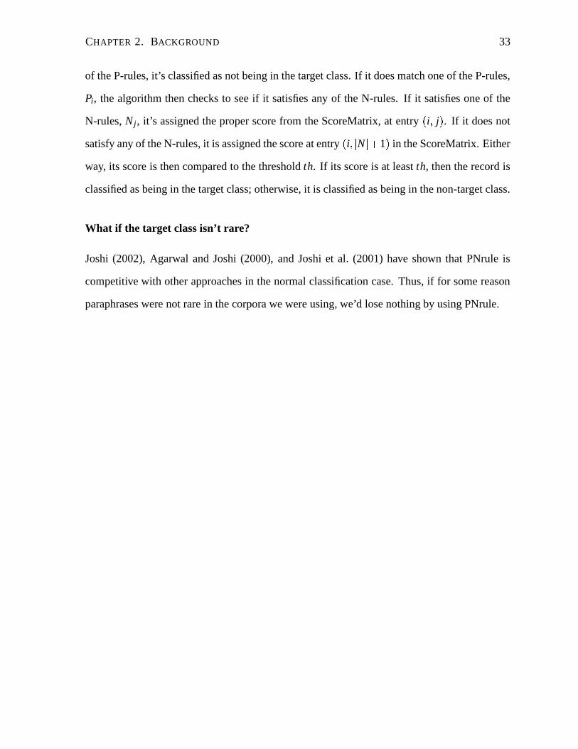
CHAPTER 2. BACKGROUND 33
of the P-rules, it’s classified as not being in the target class. If it does match one of the P-rules,
Pi, the algorithm then checks to see if it satisfies any of the N-rules. If it satisfies one of the
N-rules, N j, it’s assigned the proper score from the ScoreMatrix, at entry � i � j � . If it does not
satisfy any of the N-rules, it is assigned the score at entry � i � �N ��� 1 � in the ScoreMatrix. Either
way, its score is then compared to the threshold th. If its score is at least th, then the record is
classified as being in the target class; otherwise, it is classified as being in the non-target class.
What if the target class isn’t rare?
Joshi (2002), Agarwal and Joshi (2000), and Joshi et al. (2001) have shown that PNrule is
competitive with other approaches in the normal classification case. Thus, if for some reason
paraphrases were not rare in the corpora we were using, we’d lose nothing by using PNrule.

Chapter 3
Related Work
In this section, we review several systems, both supervised and unsupervised, that detect para-
phrases as part of their operation. Most of them (Shinyama et al. (2002), Barzilay and Lee
(2003), Quirk et al. (2004)) do so in order to discover rules for rewriting text units; one of
them (Barzilay and Elhadad (2003)) detects them as its main function. We also review the
PASCAL Recognizing Textual Entailment Challenge; as paraphrasing is a type of entailment,
the systems submitted to this challenge are also worth reviewing.
3.1 Shinyama, Sekine, and Sudo 2002
Shinyama et al. developed a method to automatically build paraphrases for a particular domain
using news articles from that domain. Their idea was that if two news articles described the
same event, then if a sentence from one article had the same named entities as a sentence in
the other article, one of those sentences was likely to be a paraphrase of the other. They were
looking at news articles written in Japanese.
Their algorithm worked as follows. They used two newspapers. First, they used a stochastic
information-retrieval system developed by Murata et al. (1999) to find articles for a particular
domain written for a single newspaper. Then, they took the top 300 relevant articles, and
tried to find articles about the same event in another newspaper. They did so, for each relevant
34

CHAPTER 3. RELATED WORK 35
article, by finding the similarity between it and every article available from the other newspaper.
Then they took the article with the highest similarity, assuming its similarity passed a certain
threshold, and paired it with the relevant article.
To obtain this similarity value, they first tagged the named entities in each article, using a
simple tagger that tagged any word not found in a dictionary of common nouns. They then
used a similarity measure developed by Papka et al. (1999) for the purpose of Topic Detection
and Tracking:
Sa � a1 � a2 � � cos �W1 � W2 �W i
k � T Fk � wi ��� IDF � wi �T Fk � wi � � fk � wi �
fk � wi � � 0 � 5 � 1 � 5 � length � k �avgdl
IDF � wi � � log � C �0 � 5
d f � wi � �log � C � 1 �
W1 and W2 are vectors containing elements W i1 and W i
2, for articles a1 and a2 respectively. Each
wi represents a named entity. fk � wi � is the number of times wi appears in article ak. d f � wi � is
the number of articles wi appears in at least once. length � ak � is the length of article ak, avgdl
is the average document length, and C is the number of articles.
Once they had the article pairs, they ran an IE pattern acquisition system, developed by
Sudo and Sekine (2001), on each of the articles. This system performed named entity tagging
and dependency analysis. This gave it a dependency tree, which it then picked paths from to
create IE patterns. Shinyama et al. used the patterns that are created more than once, and that
contained at least one named entity. An example of four IE patterns can be seen in Figure 3.1.
Next, they looked at each pair of articles and again tagged the named entities, this time
using a statistical tagging system developed by Uchimoto et al. (2000). They then applied
a morphological analyzer, Juman (Kurohashi and Nagao, 1999), and a dependency analyzer,
KNP (Kurohashi and Nagao, 1994), to each of the sentences. This output a set of dependency
trees, with the named entities tagged. They then applied the IE patterns to each of the sentences,

CHAPTER 3. RELATED WORK 36
Figure 3.1: An example of four IE patterns, obtained from a single sentence. This example was
taken from Shinyama et al. (2002).
dropping the sentences if there was no match, and filling the variables of the matching pattern
with the appropriate named entities if there was a match.
Now that they had pairs of similar articles, the authors wanted to find those sentences in
one article that were similar to sentences in the other article. Again, they based their similarity
measure on named entities, penalizing frequently occurring ones using t f � id f . This time,
however, instead of looking for exact matches, they looked for comparable named entities.
When looking at the similarity between articles, it makes sense to use exact matches between
named entities, as it’s highly likely that the same entity will be named in the same way at least
once in both articles. However, this is not the case with sentences: it’s highly likely that even if
the same entity is named, it will not be named in the same manner. For instance, one sentence
may refer to a “Mr. Suzuki,” while another sentence may refer to the same person as “Wataru
Suzuki.” The authors defined two named entities as comparable if one entity began with at least
half of the beginning string of the other (this makes sense in Japanese, where last names are
printed before any first names, titles, etc.—in a Japanese article, our two sentences would’ve

CHAPTER 3. RELATED WORK 37
Figure 3.2: An example of paraphrase extraction, taken from Shinyama et al. (2002).
referred to the same person as “Suzuki-san” and “Suzuki Wataru”). Given a sentence s1 from
article a1, and a sentence s2 from article a2, their sentence similarity measure was as follows:
Ss � s1 � s2 � � cos �W1 � W2 �W i
k � T Fk � wi � � IDFk � wi �T Fk � wi � � fk � wi �
IDFk � wi � � log � Ck
d fk � wi � �W1 and W2 are vectors containing elements W i
1 and W i2, for sentences s1 and s2, respectively. wi
is, again, a named entity. fk � wi � is the number of named entities comparable to wi that appear
in sentence sk. d fk � wi � is the number of sentences in article ak that contain at least one named
entity that is comparable to wi. Ck is the number of named entities in article ak.
The authors picked as pairs any two sentences with similarity above a certain threshold.
Recall that each sentence had at least one IE pattern associated with it. If a pattern associated
with one sentence had the same number of comparable named entities as a pattern associated
with the other sentence, the two patterns were linked as paraphrases. An example of this
process can be found in Figure 3.2.
In order to test their algorithm, the authors used one year’s worth of articles from two

CHAPTER 3. RELATED WORK 38
Japanese papers, Mainichi and Nikkei. They looked at two domains: arrest events, which they
defined as articles about arresting robbery suspects, and personnel affairs, which they defined
as articles about the hiring and firing of executives. They managed to obtain 294 pairs of
articles in the arrest events domain, and 289 in the personnel affairs domain. They then ran
the pattern acquisition system, and obtained 725 patterns in the arrest events domain and 157
in the personnel affairs domain. Using these patterns, they obtained 53 arrest-events-domain
paraphrase pairs and 83 personnel-affairs-domain pairs.
In order to evaluate the precision and coverage of their method, the authors first split the IE
patterns into clusters. Each cluster contained patterns that described the same event and that
captured the same information. If a cluster contained only a single pattern, that pattern was
dropped. This left the authors with 393 patterns in 111 clusters for the arrest events domain,
and 129 patterns in 20 clusters for the personnel affairs domain. Recall that at this point, some
of the patterns had been paired with others, and were considered paraphrases of one another. In
order to determine precision, a pairing was considered correct if both patterns were in the same
cluster. For the arrest events domain, this was true for 26 out of the 53 pairs, giving a precision
of 49%. For personnel affairs, it was true for 78 out of 83 pairs, which gave a precision of 94%.
In order to determine coverage, the authors first represented each of these clusters as a
graph, with the patterns as nodes and their pairings as edges. Ideally, each graph should have
been connected; there should have been a path between any two nodes in the cluster. The
authors were able to get an estimation of coverage by looking at the number of edges necessary
to make the graphs connected. They defined L � ∑ni � 1 � si � 1 � as the additional links necessary
to make the graphs connected, where si is the number of connected components in cluster i.
Let pi be the number of patterns in a cluster i. Then M � ∑ni � 1 � pi � 1 � is the total number of
necessary edges to make each cluster a complete graph. The authors thus defined coverage as
C � 1 � LM . For the arrest events domain, the authors needed to add 230 new edges to obtain
the necessary 252 edges to make each cluster a complete graph, which gave them a coverage of
9%. For the personnel domain, the authors needed 57 new edges to obtain a total of 109 edges,

CHAPTER 3. RELATED WORK 39
Figure 3.3: Example of paraphrase patterns obtained by Shinyama et al. (2002), taken from
that paper.
which gave them a coverage of 47%.
3.2 Barzilay and Lee 2003
Barzilay and Lee developed a method to extract automatically paraphrase patterns from an
unannotated corpus, and then to use those patterns to create new paraphrases. Specifically,

CHAPTER 3. RELATED WORK 40
they looked at sentence-level paraphrases, which, as they state, cannot be constructed by sim-
ply combining lexical paraphrases. As with Shinyama et al., they were looking at news articles
about the same event, although they drew their articles from two newswire agencies instead of
two newspapers. They claim that their method allowed them to extract paraphrases that bear lit-
tle surface resemblance to one another. In addition, their method allowed them to acquire some
paraphrases from each individual corpus, although these paraphrases had to be very similar in
structure.
The first step in their algorithm was to cluster the sentences in the corpora. They began
by preprocessing the sentences, replacing all dates, proper names, and numbers with generic
tokens. Next, they did a hierarchical complete-link clustering, using a similarity measure based
on the word n-gram overlap of the sentences. The idea was that within a cluster, the sentences
should describe similar events and should have similar structures.
The next step was to induce patterns that could be used to build paraphrases. First, the
authors created a word lattice by using iterative pairwise alignment on the sentences. There is a
method known as pairwise multiple-sequence alignment that takes two sentences and a scoring
function that gives a similarity measure between two words, and determines the highest scoring
way to transform one sentence into the other, using insertions, deletions, and transformations.
Iterative pairwise alignment is an extension of this method to multiple sentences. Figure 3.4
contains an example of a word lattice.
Each path through a word lattice corresponds to a sentence. Thus, using this lattice, the
authors could create as many sentences as the lattice had paths through it, including some
sentences that they had not necessarily seen before. For example, look at Figure 3.4. Two of
the paths through this lattice might correspond to sentences found in the corpus, for instance:
a. A suicide bomber blew himself up in the coastal resort of NAME on DATE killing
NUM other people as well as himself and wounding NUM more.
b. A Palestinian suicide bomber blew himself up in a garden cafe on DATE killing
himself and injuring NUM people.

CHAPTER 3. RELATED WORK 41
Figure 3.4: An example of a a word lattice obtained using pairwise multiple-sequence align-
ment, and the same lattice after parts of it have been replaced by slots. This example was taken
from Barzilay and Lee (2003).
By following parts of each of these two paths, we can get a sentence such as: A Palestinian
suicide bomber blew himself up in a garden cafe on DATE killing NUM people as well as
himself and injuring NUM more.
However, there was still no way to use this lattice to paraphrase a sentence that contained
words not in the lattice, even if the structure and meaning of the sentence was close to those
of the sentences represented by the lattice. The authors needed some way to determine which
words were not vital to the structure of the lattice, but were instead instances of arguments.
The authors hypothesized that areas of large variability within the lattice corresponded to argu-
ments, and should be replaced with slots, which could be filled by any instance of an argument.
In order to identify what parts of the lattice ought to be replaced by slots, the authors first
identified those nodes that were clearly not arbitrary. They called these backbone nodes, and
defined them as those nodes shared by at least 50% of the sentences from which the lattice
was induced. If one of the backbone nodes contained one of the generic markers they used to
replace proper names, dates, and numbers, it was replaced with a slot.
Now that they had identified the backbone nodes, the authors wanted to distinguish between
variations caused by synonyms, and those caused by arguments. They wanted to preserve those
parts of the lattice caused by the former, while replacing those caused by the latter with slots.
To achieve this, they tuned a threshold s (in this case, it was tuned to 30): if less than s% of

CHAPTER 3. RELATED WORK 42
the edges out of a backbone node led to the same node, a slot node was inserted after that
backbone node. Also, any node that had less than s edges leading into it was dropped, under
the assumption that it was probably an idiosyncrasy.
At this point, the authors paired the lattices by comparing the slot values of cross-corpus
sentence pairs that appeared in articles written on the same topic on the same day. The lattices
were paired if the degree of matching was over a tuned threshold. The similarity measure
was based on word overlap. It gave double weight to proper names and numbers, and ignored
auxiliaries.
Given a sentence, the authors would first find the lattice to which the sentence was best
aligned. First, “insert” nodes were added between backbone nodes; these could match any
word sequence, which allowed the system to handle previously unseen words. Then, they
performed multiple-sequence alignment where insertions were scored as � 0 � 1 and all other
node assignments were scored as 1. After this was accomplished, the authors could generate
paraphrases by filling in the slots of the best-aligning lattice’s pair with the arguments from the
sentence. This gave as many paraphrases as there were paths through the paired lattice.
In order to evaluate their algorithm, the authors used articles written between September
2000 and August 2002 from Agent France-Presse and Reuters. Using a document-clustering
system, they collected 9MB of articles on acts of violence in Israel and army raids on Pales-
tinian territory. Of these articles, 120 were held out for parameter training.
The algorithm extracted 43 slotted lattices from the AFP corpus, and 32 from Reuters. It
found 25 cross-corpus matching pairs of lattices. A path through a lattice can be considered a
paraphrase template: it consists of backbone nodes and nodes where arguments can be placed.
Since each lattice contains multiple paths, the 25 lattice pairs yielded a total of 6,534 template
pairs. These templates were judged by four native speakers of English who were unfamiliar
with the system. Given a pair of templates, the judges were told to mark them as paraphrases
if, for many instantiations of the variables, the resulting text units were paraphrases of one
another. The authors randomly extracted 250 template pairs. 50 of those pairs were evaluated

CHAPTER 3. RELATED WORK 43
Table 3.1: Two example sentences and generated paraphrases taken from Barzilay and Lee
(2003). Baseline was achieved by simply replacing words with randomly-chosen WordNet
synonyms. The judges felt that the MSA algorithm preserved meaning for example 1, but not
2, and that the baseline did not preserve meaning in either case.
by all 4 judges; the other 200 were split into 4 groups of 50 pairs, and each judge was given a
different group of 50. The Kappa score on the 50 common pairs was 0.54. Each judge gave a
different validity score: 68%, 74%, 76%, and 96%.
The authors also evaluated the quality of the resulting paraphrases. They randomly selected
20 AFP articles about violence in the Middle East. Out of the 484 sentences contained in these
articles, they found they were able to paraphrase 59 (12.2%) of them. The authors noted
that once proper-names were substituted back in, only seven of the paraphrasable sentences
were found in the training set, which indicates that generalization did occur. Interestingly, the
authors found that they were more likely to find paraphrasable sentences in shorter articles, as
longer articles were more likely to contain unique information. This time, two judges were
used to evaluate the quality of the paraphrase pairs. They had a Kappa score of 0.6, with one
judge evaluating 81.4% of the pairs as correct, and the other 78%.
3.3 Barzilay and Elhadad 2003
Like us, Barzilay and Elhadad wanted to identify pairs of sentences that contain clauses con-
veying the same information. In order to do so, they developed a method of sentence alignment
for monolingual comparable corpora. Sentence alignment works by first computing the local

CHAPTER 3. RELATED WORK 44
Figure 3.5: While both of these sentence pairs have the same similarity value, the first pair
are paraphrases of one another, while the second pair are not. This example was taken from
Barzilay and Elhadad (2003).
similarity for each sentence, and then finding an overall sequence of mapped sentences, using
the local similarity of the sentences as well as other attributes. To illustrate why a local simi-
larity value alone is not sufficient, Barzilay and Elhadad (2003) give the example in Figure 3.5.
Despite the fact that both pairs of sentences have the same number of matching word pairs, the
first pair are paraphrases of one another, while the second pair are not.
Traditionally, sentence alignment has been used on parallel multilingual corpora. In such
corpora, there are minimal insertions and deletions, and the information appears in roughly
the same order in the two texts. In contrast, comparable corpora tend to contain a lot of noise.
There may be a great deal of information appearing in one text that does not appear in the other,
and there is no guarantee as to what order that information will appear in. Thus, the authors
had to develop a new method of sentence alignment, specifically designed for monolingual
comparable corpora.
The authors based their approach on a theory called Domain Communication Knowledge.
This theory states that within a particular domain and genre, texts draw from a limited set of
topics. Texts also have a topical structure: roughly speaking, the sentences within a particular
paragraph will tend to be on the same topic. Thus, one can look at the context of two sentences
to help determine whether or not they should be aligned. If two sentences appear within con-
texts that fall within the same topic, they are more likely to be aligned than if they fall within

CHAPTER 3. RELATED WORK 45
unrelated topics.
With this in mind, the first thing the authors had to do was find some way to decide whether
a paragraph in one corpus fell within the same topic as a paragraph in the other corpus. They
decided to use a two-step process: first, they placed the paragraphs of each corpus into topic
clusters; then, informed by these clusters, they found a mapping between the paragraphs of
one corpus and those of the other. To accomplish the first step, they began by replacing proper
names, dates, and numbers with generic tags. This was important, because they were trying
to cluster by the type of information provided, not by the subject of that information. Next,
they did a hierarchical complete-link clustering of the paragraphs, using the cosine similarity
measure based on the matching of content words. This gave them their topic clusters for each
corpus.
For the purposes of training, they considered two paragraphs to map to one another if
they contained at least one aligned sentence pair. To map the paragraphs, the authors used a
supervised approach. For their training set, they used a set of manually aligned text pairs from
the corpora. They then used BoosTexter (Singer and Schapire, 1998), iterating 200 times, to
train a model to classify two paragraphs, P and Q as mapping or not mapping based on their
lexical similarity (again, cosine similarity based on word overlap), the cluster number of P, and
the cluster number of Q. An example of two paragraphs that mapped to one another can be
seen in Figure 3.6.
Given this model, sentence alignment worked as follows: given two texts, sentences with
high lexical similarity ( � � 5) were aligned. Then, for each paragraph, the cluster it was closest
to was found. Each paragraph in one text was mapped to the other text’s paragraphs using the
classification scheme mentioned above. Within each pair of mapped paragraphs, dynamic pro-
gramming was then used to compute local alignments. The idea was that given two sentence
pairs with moderate lexical similarity, whether or not they should be aligned could be deter-
mined by looking at whether they were near to other sentence pairs with high lexical similarity.

CHAPTER 3. RELATED WORK 46
Figure 3.6: An example of two paragraphs that mapped to one another, taken from Barzilay
and Elhadad (2003).
Thus, given two sentences, i and j, their local similarity value was:
sim � i � j � � cos � i � j � � mismatch penalty
The mismatch penalty was used to further penalize sentence pairs with low similarity measures.
The weight of the optimal alignment between two sentences was computed as:
s � i � j � � max
���������������� ���������������
s � i � j � 1 � � skip penalty
s � i � 1 � j � � skip penalty
s � i � 1 � j � 1 � � sim � i � j �s � i � 1 � j � 2 � � sim � i � j � � sim � i � j � 1 �s � i � 2 � j � 1 � � sim � i � j � � sim � i � 1 � j �s � i � 2 � j � 2 � � sim � i � j � 1 � � sim � i � 1 � j �
The skip penalty was used to stop only those sentence pairs with high similarity from being
aligned. Unfortunately, this weight measure appears to be a recursion without a halting condi-
tion; however, we have printed it exactly as it appears in Barzilay and Elhadad (2003).
In order to evaluate their method, Barzilay et al. used as corpora the Encyclopedia Bri-
tannica and the Britannica Elementary. They picked 103 pairs of city descriptions, held out

CHAPTER 3. RELATED WORK 47
Figure 3.7: An example of two alignments found by this method, taken from Barzilay and
Elhadad (2003). The first alignment is incorrect, while the second is correct.
11 for testing, used the other 92 for vertical clustering into 20 clusters, and then of those 92
pairs, used 9 for training. They had each pair in the training and testing set annotated by two
annotators. The sentences in each pair were considered to be aligned if they both contained at
least one clause that expressed the same information. Many-to-many alignments were allowed.
Once the two annotators were finished, a third annotator judged any contested pairs. 320 pairs
were aligned in the training set, out of a total of 4192 sentence pairs, and 281 were aligned in
the testing set, out of a total of 3884 pairs.
By varying the mismatch penalty from 0 to 0.45, and using a skip penalty of 0.001, the
authors were able to get a range of recall from 25% to 65%. At 55.8% recall, they obtained
76.9% precision.
One point we’d like to address is Barzilay and Elhadad’s (2003) criticism of Hatzivas-
siloglou et al. (2001). Like us, Hatzivassiloglou et al. (2001) use a machine-learning algorithm
with various lexical features, although they use it to find similar text passages (where similarity
includes, but is not limited to, paraphrasing) instead of clause-level paraphrases. Barzilay and
Elhadad claim that their results, and the fact that Hatzivassiloglou et al.’s system, SIMFINDER,
does not perform as well on the same test data, proves that it is better to use an approach with
a simple local similarity combined with a simple global similarity, instead of an approach with
a set of complex lexical features and a machine-learning algorithm. There are two problems
with this conclusion: first, SIMFINDER was trained on news articles, not encyclopedia entries,

CHAPTER 3. RELATED WORK 48
so it’s hardly surprising that it wouldn’t perform as well on the test data; second, Barzilay and
Elhadad are able to obtain 55.8% recall and 57.9% precision on their test data by doing nothing
more than seeing if the cosine similarity of two sentences is over a particular threshold. While
this does not dismiss their results—they obtain a precision of 76.9% at the same level of recall
using their system—we do question whether it’s fair to dismiss more complicated methods
based on results using a corpus where such an incredibly simple method works so well.
3.4 Quirk, Brockett, and Dolan 2004
Quirk et al. (2004) tried to infer rules for the generation of phrasal-level paraphrases from
comparable corpora. Instead of attempting to extract patterns like Shinyama et al. (2002) or
Barzilay and Lee (2003), they treated paraphrasing as a statistical machine translation problem.
Specifically, they used the noisy channel model developed by Brown et al. (1993). Given a
sentence S to be paraphrased, they wanted to find:
T � � argmaxT
�Pr � T � S � �
� argmaxT
�Pr � S �T � Pr � T � �
where T � is the optimal paraphrase of S, T is a sentence in the same language as S, Pr � S �T � is
the channel model, and Pr � T � is the target language model.
Like Shinyama et al. (2002) and Barzilay and Lee (2003), Quirk et al.’s corpus was drawn
from news articles on the same event. However, instead of drawing the articles from two news-
papers, they used online news gatherers, such as Yahoo News and Google News, to locate
clusters of articles from a variety of newspapers on the same event. Using a Hidden Markov
Model to distinguish between article content and various types of noise such as ads, they col-
lected these clusters over a period of about eight months, eventually gathering 11,162 in all,
containing a total of 117,095 articles, with an average of 15.8 articles per cluster.
In order to find pairs of sentences containing potential paraphrases of one another, they first

CHAPTER 3. RELATED WORK 49
set all of the words in the sentences to lowercase, and then found the Levenshtein edit distance1
between each pair of sentences within a cluster. They rejected duplicate pairs, pairs that were
identical or differed only in punctuation, pairs with significantly different lengths, and pairs
where the edit distance was greater than 12 � 0. This gave them a total of 139,000 non-identical
pairs.
At this point, they aligned the words of each pair of sentences using GIZA++ (Och and
Ney, 2000), which is a free implementation of IBM Models 1–5 (Brown et al., 1993) and
HMM alignment (Vogel et al., 1996). In machine translation, one would align the target text
to the source text. However, in order to capture many-to-many alignments between sentences,
the authors both aligned the target text to the source text, and aligned the source text to the
target text. They then heuristically recombined the unidirectional word alignments into a single
bidirectional alignment.
Next, they adapted a phrasal decoder patterned after that of Vogel et al. (1996) to identify
what they refer to as phrasal replacements. The decoder worked as follows: think of two
sentences, S and T , where S is the source sentence and T is the target sentence, as sequences
of words s1 � � � � � sm and t1 � � � � � tn, respectively. Then a word alignment A of S and T can be
expressed as a function from each token of S and T to a unique cept (Brown et al., 1993). A
cept is a minimal mapping between words and their positions in one sentence to words and
their positions in the other, where the two sets of words refer to the same concept. In order to
understand what we mean by “minimal”, let’s look at two sentences:
a. Four humans saw the large cat.
b. Four people saw the tiger.
In this case, (four(1) � four(1)) and (humans(2) � people(2)) would both be cepts, but (four(1)
humans(2) � four(1) people(2)) would not be. This is not to say that each component of the cept
1The Levenshtein edit distance between two strings is the number of insertions, deletions, and substitutionsrequired to transform one string into the other. For further explanation, see http://www.merriampark.com/ld.htm.
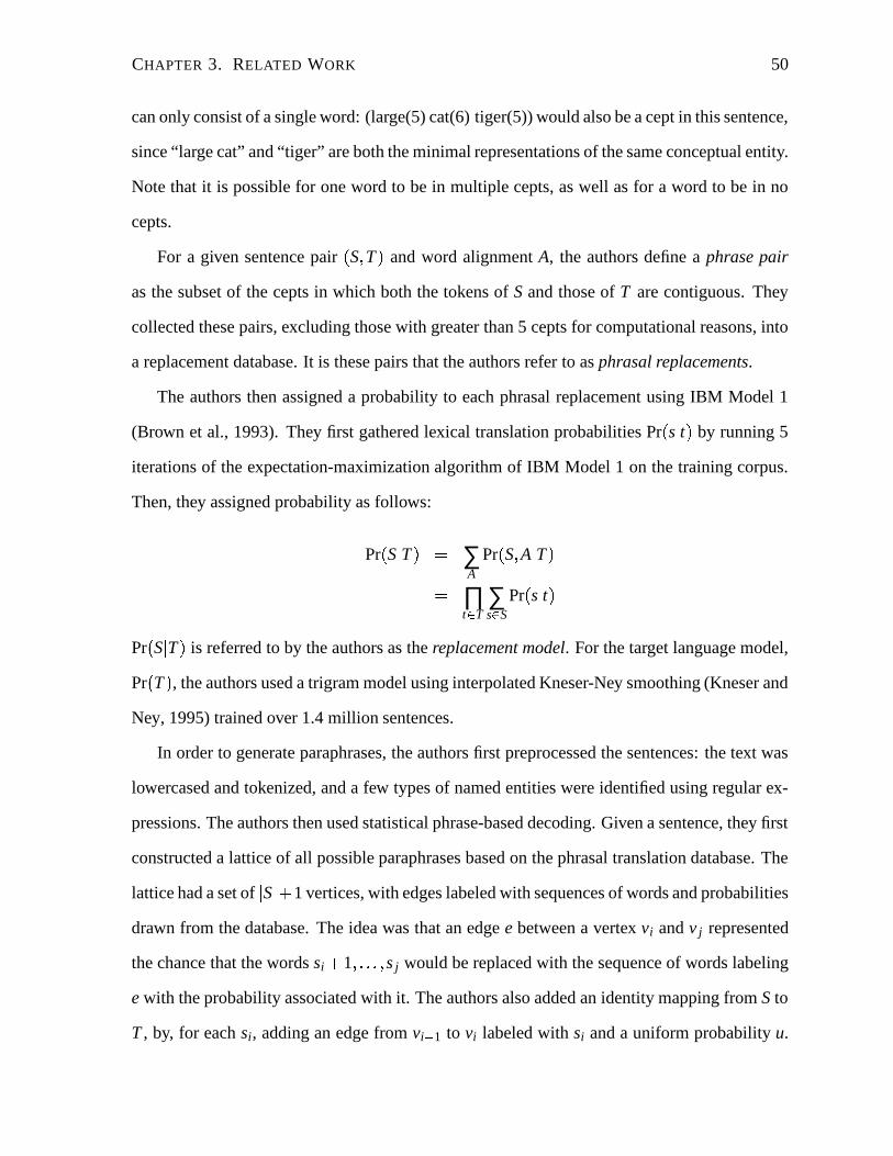
CHAPTER 3. RELATED WORK 50
can only consist of a single word: (large(5) cat(6) � tiger(5)) would also be a cept in this sentence,
since “large cat” and “tiger” are both the minimal representations of the same conceptual entity.
Note that it is possible for one word to be in multiple cepts, as well as for a word to be in no
cepts.
For a given sentence pair � S � T � and word alignment A, the authors define a phrase pair
as the subset of the cepts in which both the tokens of S and those of T are contiguous. They
collected these pairs, excluding those with greater than 5 cepts for computational reasons, into
a replacement database. It is these pairs that the authors refer to as phrasal replacements.
The authors then assigned a probability to each phrasal replacement using IBM Model 1
(Brown et al., 1993). They first gathered lexical translation probabilities Pr � s � t � by running 5
iterations of the expectation-maximization algorithm of IBM Model 1 on the training corpus.
Then, they assigned probability as follows:
Pr � S � T � � ∑A
Pr � S � A �T �� ∏
t�
T∑s � S
Pr � s � t �Pr � S �T � is referred to by the authors as the replacement model. For the target language model,
Pr � T � , the authors used a trigram model using interpolated Kneser-Ney smoothing (Kneser and
Ney, 1995) trained over 1.4 million sentences.
In order to generate paraphrases, the authors first preprocessed the sentences: the text was
lowercased and tokenized, and a few types of named entities were identified using regular ex-
pressions. The authors then used statistical phrase-based decoding. Given a sentence, they first
constructed a lattice of all possible paraphrases based on the phrasal translation database. The
lattice had a set of � S � � 1 vertices, with edges labeled with sequences of words and probabilities
drawn from the database. The idea was that an edge e between a vertex vi and v j represented
the chance that the words si � 1 � � � � � s j would be replaced with the sequence of words labeling
e with the probability associated with it. The authors also added an identity mapping from S to
T , by, for each si, adding an edge from vi � 1 to vi labeled with si and a uniform probability u.

CHAPTER 3. RELATED WORK 51
Figure 3.8: An example of a translation lattice, without the assigned probabilities, taken from
Quirk et al. (2004).
This has two effects: it allowed the method to handle unseen words, by simply keeping those
words, and, if u was set to a high value, it encouraged conservative paraphrases.
Once this had been accomplished, the optimal paraphrase could be found by finding the
optimal path through the lattice, scored by the product of the replacement model and the lan-
guage model. This was accomplished using the Viterbi algorithm. Finally, there was some
post-processing done on the paraphrase, which restored named entities and casing.
The authors noted that as this model relied on simply replacing a sequence of words with
another sequence of words, it could not handle intra-phrasal reordering. Thus, it could not
capture, for instance, active-passive alternation. However, it was able to capture synonymy
(e.g., injured/wounded), phrasal replacements (e.g., Bush administration/White House), and
intra-phrasal re-orderings (e.g., margin of error/error margin).
Quirk et al. evaluated two things: first, how well GIZA++ did word alignment between
sentence pairs, and second, how acceptable the paraphrases their method produced were. To
evaluate the former, they followed the method of Och and Ney (2003). First, they held out a
set of news clusters from their training set. From these clusters, they randomly extracted 250
sentence pairs with edit distances between 5 and 20 for evaluation. Each pair was checked by
an independent evaluator to make certain they contained paraphrases. Then, two evaluators

CHAPTER 3. RELATED WORK 52
created annotations for the sentence pairs. They marked alignments as either SURE, meaning
those words must be aligned, or POSSIBLE, meaning that it is preferable, but not necessary
that those words be aligned. Given that A is the set of all alignments, S is the set of SURE
alignments, and P is the union of the set of all SURE alignments with the set of all POSSIBLE
alignments, precision, recall, and alignment error rate (AER) are determined as follows:
��������� � � � ��A � P ��A �
����������� ��A � S �� S �
������
� A � P � � �A � S �� A � � � S �
Measured by AER, the agreement between the two annotators was 93.1%. Overall, AER
was 11.58%, with an AER of 10.57% on identical words and an AER of 20.88% on non-
identical words.
In order to judge the quality of the paraphrases generated by their method, the authors used
as a test set the 59 sentences used in Barzilay and Elhadad (2003), and 141 randomly selected
sentences from the held-out part of their corpus. For each sentence, two judges decided whether
the sentence generated by the algorithm was indeed a paraphrase of the original sentence. The
first time, the judges had an agreement rating of 84%. The authors decided this was too low,
so they had the two judges look at any examples upon which they disagreed. This led to an
agreement of 96.9%. The system was able to generate a paraphrase for all 200 sentences; the
best-scoring paraphrases received a 91.5% acceptance rate for the 59 sentences from Barzilay
and Lee (2003), and an 89.5% acceptance rate for all 200 sentences. It’s worth noting that while
this method achieved excellent coverage and acceptability, the changes were often relatively
minor, such as replacing a word or a phrase will a similar word or phrase. The average edit
distance of the paraphrases produced by this system was 2.9, as opposed to 25.8 for Barzilay
and Lee (2003).

CHAPTER 3. RELATED WORK 53
3.5 The PASCAL Recognizing Textual Entailment Challenge
3.5.1 The challenge
Since we began this project, there has been a considerable amount of publication on a related
topic: textual entailment. Textual entailment is a directional relationship between two units
of text: given two text units, t1 and t2, we say that t1 entails t2 if we can infer t2 from the
information given to us by t1. This is relevant to us because, by the definition of entailment, if
a text t2 is a paraphrase of a text t1, it must also be entailed by t1. Note that the reverse is not
true: The man murdered Bob entails Bob is dead, but Bob is dead is not a paraphrase of The
man murdered Bob.
Much of the recent work on entailment has come about due to the Recognizing Textual En-
tailment Challenge, put out by the PASCAL Network of Excellence (Dagan et al., 2005). This
challenge consists of a dataset of 567 development examples and 800 test examples that has
been designed to reflect the occurrence of entailment within several common NLP tasks. These
tasks are: question answering, information extraction, machine translation, paraphrase acqui-
sition, information retrieval, comparable documents (this was the authors’ term; “sentence
alignment of comparable documents” might be more accurate), and reading comprehension.
An example consists of a text unit t and a hypothesis unit h; the text is one or two sentences
(usually one), while the hypothesis is a shorter sentence. Each example was annotated by two
annotators, who were told to label an example as true if it was very probable that h could be
inferred from t. An example of a very probable positive example given in Dagan et al. (2005)
is as follows:
Text: The two suspects belong to the 30th Street gang which became embroiled in one of the
most notorious recent crimes in Mexico: a shootout at the Guadalajara airport in May,
1993, that killed Cardinal Juan Jesus Posadas Ocampo and six others.
Hypothesis: Cardinal Juan Jesus Posadas Ocampo died in 1993.

CHAPTER 3. RELATED WORK 54
As Dagan et al. (2005) explain, it’s possible that Ocampo died months later, in 1994, from the
wounds he sustained in 1993, but it’s very likely that he died in the same year that the shootout
occurred.
The annotators were told to ignore tense, due to the fact that the text and hypothesis were
sometimes drawn from different documents, which could have been written at different times.
Any examples upon which the two annotators disagreed were discarded, as were some exam-
ples that one of the organizers thought might be too controversial. The final corpus was built
in such a way as to have an even number of positive and negative examples. Other annota-
tors, who were not involved in the original annotation, also replaced anaphora with appropriate
references, and shortened some of the hypotheses and texts to reduce complexity.
Here’s a brief run-down of how examples were obtained for each of the various tasks:
Information Retrieval: Hypotheses look like IR queries, and were selected by examining
prominent sentences in news stories; texts were selected by putting hypothesis into
search engine and selecting from retrieved documents.
Comparable Documents: Pairs were selected by examining aligned sentences from clusters
of similar news stories found in Google news; they were also drawn from an existing
corpus of aligned sentences (probably that of Barzilay and Elhadad (2003), although it’s
a bit unclear from the paper).
Reading Comprehension: Texts were selected from news stories; hypotheses were written by
annotators, with the instruction that they should be like reading comprehension examples
found in high school tests (or, for that matter, the SATs).
Question Answering: Questions were mostly drawn from the CLEF-QA (Magnini et al.,
2003) and TREC (Voorhees, 2004) datasets, although annotators could write their own;
they inserted the questions into the TextMap Web-Based Question Answering system
(Echihabi et al., 2003) and used the results as the texts; they then rewrote the questions
as affirmative statements and used these as the hypotheses.

CHAPTER 3. RELATED WORK 55
Information Extraction: Examples were drawn from a dataset produced by Roth and Yih
(2002) and from news stories; texts were sentences in which particular relations held,
and hypotheses were the relations with their slots filled in.
Machine Translation: Examples were drawn from two translations of the same text, one au-
tomatic and the other done by a human; half of the time the hypothesis was taken from
the automatic translation and the text from the human translation, and the other half of
the time the reverse was done. Some of the automatic translations were rewritten so as
to be grammatically correct.
Paraphrase Acquisition: Texts were drawn from news stories that contained particular rela-
tions; hypotheses were created by drawing paraphrases from a paraphrase-acquisition
system (probably Lin and Pantel (2001), although again, it’s a little unclear) and by then
applying those paraphrases to the original text.
So how does the goal of this challenge differ from that of our thesis? First, as stated above,
entailment includes relationships other than paraphrases. Second, systems designed for the
RTE challenge only have to do one-way matching: they know ahead of time which text unit is
the text and which is the hypothesis. Our system, on the other hand, does not know which of the
sentences in a given pair may contain the paraphrase (if either), and which is the “original” text.
Also, in the RTE challenge, there can be no information in the hypothesis that is not included in
the text; for us, there may be clauses in either of the sentences that have no correlating clause in
the other sentence. Finally, the RTE challenge uses a corpus primarily drawn from newspaper
stories; this allows the systems designed for the challenge to use a number of tools, such as
parsers and chunkers, that have been trained on newspaper corpora.
All of that said, the goal of the PASCAL RTE challenge is still close enough to our own
that we can learn from the various systems submitted for it. Below, we give a brief overview
of these systems.

CHAPTER 3. RELATED WORK 56
3.5.2 The systems
Roughly speaking, the systems submitted to the PASCAL RTE challenge can be placed into
two groups: those that attempt to logically infer the hypothesis from the text, and those that
use some other method to detect entailment. The systems in the former group include those
of Akhmatova (2005), Bayer et al. (2005) (system 1), Bos and Markert (2005) (system 2),
de Salvo Braz et al. (2005), Fowler et al. (2005), and Raina et al. (2005) (system 2).
Akhmatova (2005)’s system works by first transforming the text and the hypothesis into a
series of atomic propositions, and then for each of the hypothesis propositions, attempting to
find a text proposition that entails it. In order to do the transformation, the system uses a link
parser and then a semantic analyzer. To find entailment between propositions, it uses an auto-
mated deduction system called OTTER (McCune, 2004). It is aided in this by some hand-coded
logic rules—including representations of equivalence, hypernymy, lexical relations, and syn-
tactical equivalence, among other relations—and by a WordNet relatedness algorithm, which is
used if no exact entailment can be found for a proposition (presumably some sort of threshold
is used, although the author doesn’t describe this). Entailment holds for the text/hypothesis
pair if all of the hypothesis propositions are entailed by text propositions.
Bayer et al. (2005) (system 1) transform the text and the hypothesis into logic proposi-
tions, and then use the EPILOG event-oriented probabilistic inference engine (Schubert and
Hwang, 2000), aided by a few hand-crafted inference rules and by simple word lists, to deter-
mine whether the hypothesis is entailed by the text. To transform the text and the hypothesis,
they do a lot of pre-processing: the text and the hypothesis are tokenized, segmented, tagged
with parts-of-speech, morphologically analyzed, and parsed with a link parser. They are then
processed by a dependency analyzer and by a Davidsonian logic generator, which outputs them
in propositional form.
Bos and Markert (2005) (system 2) also transform the text and the hypothesis into propo-
sitions, and use these along with background-knowledge axioms (bk) to attempt to prove en-
tailment. An example can be marked positive one of three ways: a theorem prover, Vampire

CHAPTER 3. RELATED WORK 57
(Riazanov and Voronkov, 2002), finds entailment; a model builder, Paradox (Claessen and
Sorensson, 2003) finds a model for the negation of entailment; or the difference in the sizes
of the model of � bk � t � and the model of � bk � t � h � is under some threshold. The authors
use a CCG-parser to parse the text and the hypothesis into propositions, and use three sources
for the background knowledge: the semantics of certain types of words and relationships; lex-
ical knowledge created using WordNet hypernyms; and geographic knowledge from the CIA
factbook. They combine these features with those of system 1 (described below) by training a
decision tree classifier over them.
De Salvo Braz et al. (2005), Fowler et al. (2005), and Raina et al. (2005) (system 2)
all use a method known as “extended unification”: if two terms cannot be unified, the rules
governing unification are relaxed. Each type of relaxation that can occur is assigned a cost,
and at the end the total cost of unification is compared against some threshold; if the cost is
below that threshold, the example is marked as positive (this is how both de Salvo Braz et al.
(2005) and Raina et al. (2005) work; Fowler et al. (2005) actually assigns higher scores to
those examples which require less relaxation of terms, and then checks to see if the total score
is over a threshold, but the basic idea is still the same).
De Salvo Braz et al. (2005) use Extended Feature Description Logic to represent the text
and hypothesis (augmented with syntactic and semantic parses), as well as a series of syn-
tactic and semantic rewrite rules. The representations of the text and of the hypothesis are
hierarchical—this allows the rewrite rules to depend on levels higher than lexical—and are
created using a tokenizer, a lemmatizer, a part-of-speech tagger, a syntactic parser, a semantic
parser, a named entity recognizer, and a name coreference system. Some of the rewrite rules
are taken from Lin and Pantel (2001); others have been manually generated. The system uses
these rewrite rules to create several alternative representations of the text. For each of these
representations, it attempts to unify the hypothesis into the representation, using extended uni-
fication. The unification process is a bit complicated, but the idea is basically this: first, they
make sure that for each verb in the hypothesis, there is a verb in the text with the same attribute

CHAPTER 3. RELATED WORK 58
set and arguments at both the semantic role and syntactic parse levels. If every verb in the hy-
pothesis has a matching verb in the text, then the cost is set to zero; otherwise, the cost is set to
infinity. Assuming the cost has not been set to infinity, the system goes on to recursively match
phrase-level nodes, penalizing nodes that do not match by assigning them a uniform cost, and
then to match word-level nodes, again penalizing nodes that do not match by assigning them a
uniform cost; this gives the system the total unification cost.
Fowler et al. (2005) use part-of-speech tagging, parse-tree generation, word-sense disam-
biguation, and semantic-relations detection to convert the text and the hypothesis into logical
forms—although they ultimately remove the word senses from the predicates, as it turns out
that the disambiguator is rather inaccurate. To prove entailment, they use COGEX (Moldovan
et al., 2003), a modified version of OTTER (McCune (2004); the prover used by Akhmatova
(2005)). COGEX is fed the negated form of the hypothesis, the text, and a set of axioms that
include world knowledge, knowledge of syntactic equivalence, and lexical chains. In order
to successfully complete unification, COGEX is allowed to use these axioms, to relax predi-
cate arguments, and to drop predicates. The example is then scored depending on how many
of these actions take place during the proof process—the more that take place, the lower the
score. The score is normalized by calculating the maximum penalty that can be assigned and
then dividing by this number.
Raina et al. (2005) (system 2) transforms the text and the hypothesis into logical formu-
las that capture their respective syntactic dependencies. In order to unify each term of the
hypothesis with a term of the text, the system can relax unification in the following ways:
allowing terms with different predicates to be unified (with cost determined by a similarity
measure), allowing terms with different numbers of arguments to unify (with cost based on
the annotation of those arguments), and allowing constants to unify (the cost is uniform over
an example, although it is lowered if there’s a possible coreference or appositive reference);
they use a learning algorithm to determine the costs of these relaxations. This system outputs a
confidence score for each example; this is combined with a similar confidence score output by

CHAPTER 3. RELATED WORK 59
Raina et al. (2005) (system 1) using logistic regression. The authors try training the weights for
the regression in two ways: one set of weights trained over all of the examples, and a separate
sets of weights trained over the examples from each of the tasks.
The rest of the systems used a variety of approaches to the entailment problem. Pazienza
et al. (2005), Raina et al. (2005) (system 1), and Herrera et al. (2005) use dependency parsers to
transform the text and the hypothesis into graphs, then use approaches based on graph match-
ing. The goal of these systems is to maximize the similarity value between the two graphs;
this similarity value is then compared against a threshold, and if it’s greater than or equal to
that threshold, the example is marked positive. Pazienza et al. (2005) create syntactic graph
representations of the text and the hypothesis (the nodes are words or phrases, and the edges
are syntactic relationships), and then attempts to find the maximal subgraph of the hypothesis
that is in an isomorphic relationship with a subgraph of the text. An isomorphic relationship
exists between two graphs, G and H, if every node and edge in G can be subsumed by the
nodes and edges in H, and vice versa. In this system, when a node is subsumed by another
node, it is assigned a similarity value based on the semantic similarity between the two nodes;
similarly, when an edge is subsumed by another edge, it is assigned a similarity value based on
the syntactic similarity between the two edges. The calculation of the similarity between the
two graphs is based on these similarities. There are two versions of this system: in one, the
parameters used in the similarity measures are set manually; in the other, these parameters are
tuned using a support vector machine.
Raina et al. (2005) (system 1) also use graph isomorphisms, only instead of trying to find
a maximal subgraph of the hypothesis, they add a nil node to each graph and allow the nodes
of the other graph to match to it if necessary. Each node or edge subsumption is assigned a
particular cost, depending on the properties of the nodes or edges involved in the subsumption.
For node subsumption, the properties the system checks for are as follows, in order of increas-
ing cost: whether the stems of the hypothesis node and the subsumption node and their parts of
speech match; whether the stems of the two nodes match, but having different parts of speech;

CHAPTER 3. RELATED WORK 60
whether the hypothesis node is a synonym of the subsuming node; whether the hypothesis node
is a hypernym of the subsuming node; and, finally, whether the two nodes are similar according
to a word similarity module developed by the authors. Each cost is weighted by the importance
of the hypothesis node it applies to, as determined by the part-of-speech tag of the node or the
type of named entity it is; the cost is then normalized by dividing it by the total weight of the
nodes. For edges, the cost of the subsumption is determined solely by looking at the properties
of the nodes of the subsuming edge. These properties, again in order of increasing cost, are:
whether one of the nodes is a parent of the other; whether one of the nodes is an ancestor of
the other; whether the two nodes share a parent; and, whether the two nodes share an ancestor.
Again, the costs of the edge subsumptions are weighed by the importance of the edges being
substituted for, as determined by the relations those edges represent (such as subject or object).
The overall edge- and node-subsumption costs are then combined using a convex mixture; the
algorithm approximates the lowest-cost match using a combination of the Hungarian method
(Kuhn, 1955) and a greedy hill-climbing search. This system outputs a confidence score for
each of the examples, which is them combined with the output of Raina et al. (2005) (system
1), as detailed earlier.
Herrera et al. (2005) take a somewhat different approach. Their system begins by trying to
find nodes in the hypothesis that are entailed by nodes in the text: using WordNet, a hypoth-
esis node is entailed by a text node if the two nodes are in the same synset, or if, using the
hypernymy and entailment relations, a path can be found between a synset of the hypothesis
node and a synset of the text node. The system also checks for negation: in such a case, the
antonym of the node (as determined by WordNet) is used in its place in determining entailment
between nodes. Once this is accomplished, a simple matching algorithm is used, that matches
the branches of the hypothesis tree with branches in the text tree. Two branches match if each
of the nodes in the text branch entails a node in the hypothesis branch. The similarity value
between the two trees is then simply the percentage of nodes in the hypothesis tree that are part
of a branch that is matched to a branch in the text tree. The threshold used by this system is

CHAPTER 3. RELATED WORK 61
50%.
Wu (2005) uses a measure based on the Inversion Transduction Grammar Hypothesis. Pre-
viously, ITGs had been used in machine translation and alignment. Given two languages, an
input language and an output language, the ITG grammar is used to transform sentences from
the input language into sentences in the output language; in the case of this system, of course,
the input and output languages are the same. ITGs have two types of rules: straight and in-
verted. In a straight rule, the symbols on the right-hand side of the rule must be in the same
order for both languages. In an inverted rule, the symbols on the right-hand side of the rule
must be left-to-right for the input language and right-to-left for the output language. Wu (2005)
uses a special type of ITG, a Bracketing ITG. It uses only a single “dummy” non-terminal, and
thus, unlike other ITGs, it does not requiring any language-specific information; the only op-
eration it allows for is transposition of words and phrases. The examples are assigned scores
using a biparsing algorithm described in Wu and Fung (2005); we won’t get into the details of
that algorithm, but the basic idea is that those pairs of sentences that have fewer transpositions
between them are assigned a higher score. There are two runs of this system: one where the
system is run after removing words in a stoplist from the example, and one where no such
removal is performed.
Following a similar idea as Wu (2005), Bayer et al. (2005) also use a method originally
developed for machine translation—in this case, a statistical machine translation model. Like
Quirk et al. (2004), this system uses GIZA++ for its alignment models. In this case, the models
were trained on the Gigaword (Graff, 2003) corpus, using the lead paragraphs of the articles as
“texts” and their headlines as “hypotheses”. They combine the alignment model with a series
of string similarity metrics by placing the examples in a vector space and using a k-nearest-
neighbor classifier to classify them.
Glickman et al. (2005) use a generative probability model to determine the probability that
a given text entails a given hypothesis. In order to do this, they make several simplifying
assumptions: first, that the content words in a hypothesis can be assigned truth values; second,

CHAPTER 3. RELATED WORK 62
that a hypothesis is true if and only if all of its content words are true; third, that the probability
of a content word being true is independent of the truth of the other content words in the
hypothesis; and fourth, that the probability that a content word in the hypothesis is true is
primarily dependent upon a single content word in the text. The basic idea, then, is to find an
alignment between the text and the hypothesis in such a way as to maximize the probability of
entailment. In order to do this, of course, the authors need to come up with the probability that
a given content word entails another content word. To do this, they use a search engine and
maximum likelihood: given two words, n and m, the probability that n entails m is estimated
as the number of documents in which both n and m appear over the number of documents
in which n appears. Once they’ve found the best alignment and calculated its probability, the
authors compare the probability to a threshold; if it’s over that threshold, the example is marked
as positive.
Delmonte et al. (2005) use a rather complicated approach to the problem. Their system
involves two subsystems, with the output of the first subsystem piped into the second subsys-
tem. The first subsystem is relatively straightforward: it takes the text and the hypothesis as
input, and outputs a list of head-dependent structures labeled with their grammatical relations
and their semantic roles. The second subsystem either assigns a score to an example, where a
lower score is better than a higher one, or simply labels the example as false. The latter occurs
if the example fails a consistency check; these checks look for things such as the presence of
antonyms, differing time values (e.g. 1992 vs 2003), and differing locations (e.g. England
vs France). This subsystem consists of two modules. The first module consists of five sub-
calls based in linguistics; and the second module scores an example based on the number of
matching heads, dependents, grammatical relations, and semantic roles between the text and
the hypothesis. Each subcall of the first module requires certain aspects of the text and of the
hypothesis to match. The idea is to first try to find obvious cases of entailment (for exam-
ple, when only word order has been changed), and to then work down to situations where the
system has little more than a rough estimate of semantic similarity to work with. Thus, they

CHAPTER 3. RELATED WORK 63
are ordered in such a way that the earlier subcalls give lower (and thus better) costs than the
later ones, as those subcalls are also more likely to be indicative of entailment. We won’t go
into detail about all five of these subcalls, but, for example, the first subcall requires the main
predicates of the text and hypothesis to match, as well as their core arguments, although certain
semantic roles may be changed (a pair such as I killed Bob and Bob was killed by me. would fit
the requirements of this subcall). By contrast, the fifth subcall allows the main predicates to be
different, but the core arguments must be synonyms of one another, and another non-argument
head-driven structure must also be matched. For later subcalls, the second module is used to
supplement the decision. Unfortunately, the authors don’t go into detail about precisely how
the examples are scored, but ultimately they are compared against some threshold; if they score
below that threshold, they are classified as positive.
We now detail three very simple systems: Andreevskaia et al. (2005), Bos and Markert
(2005) (system 1), and Jijkoun and de Rijke (2005). Andreevskaia et al. (2005) compare Pred-
icate Argument Structures; a PAS contains a verb, its subject, and its object (if any). They
transform the hypothesis and the text into PASs by extracting the noun phrases and the verb
groups from them, and then parsing them using either the Link parser (Sleator and Temperley,
1993) or the RASP parser (Briscoe and Carroll (2002), whichever creates more PASs). They
also find coreference chains for the text and for the hypothesis, both separately and together.
Once it has the PASs, their system checks to whether a numerical value exists in the hypothesis
that does not exist in the text; if it does, it classifies the example as negative. Next, it transforms
any passive PASs into active ones, and uses WordNet to compute the distance between verbs in
the text and in the hypothesis. If this distance is below some threshold, and both verbs have sub-
jects and/or arguments, and if the corresponding subjects and/or arguments share coreferences,
then the example is classified as positive. Finally, the system checks whether the hypothesis
contains the pattern X is Y; if it does, and there exists some X � and some Y � in the text such that
X � is in the same coreference chain as X and that Y � is in the same coreference chain as Y , the
example is marked as positive. Otherwise, the example is classified as negative.

CHAPTER 3. RELATED WORK 64
Bos and Markert (2005) (system 1) is particularly simple. It first tokenizes and lemmatizes
the text and the hypothesis. Using the Web as a corpus, it assigns each lemma in the hypothesis
an IDF value. It then initializes the similarity score of the text/hypothesis pair to zero, and
looks at the word overlap between them: if a lemma in the hypothesis exists in the text, its
IDF value is added to the score; otherwise, its IDF value is subtracted from the score. The
score is then normalized by dividing it by the sum of the IDF values of the lemmatize in the
hypothesis. This normalized score, which has a value between � 1 and 1 (inclusive), is then
compared against a threshold. If it’s greater than the threshold, the example is classified as
positive; otherwise, it’s classified as negative.
Jijkoun and de Rijke (2005) use a bag-of-words approach. First, they assign each word a
weight; for this they use its normalized inverse document frequency, as calculated over a corpus
of newspaper texts. Then, for each word in the hypothesis, they use a similarity measure to find
the most similar word in the text. They try two different similarity measures: a dependency-
based measure (Lin, 1998) and a measure based on lexical chains (Hirst and St-Onge, 1998).
Starting with a total similarity score of zero, for each word in the hypothesis, they add its weight
multiplied by the similarity value of its most-similar word to the total score. If no similar word
could be found (that is, all the words in the text gave a similarity score of zero), then the weight
of the word is subtracted from the total score. The total similarity score is then normalized by
dividing it by the total weight of the words in the hypothesis. It’s then compared to a threshold,
and if it’s greater or equal to that threshold, the example is classified as positive; otherwise, it’s
classified as negative.
The final system we describe here is that of Newman et al. (2005). We left this for last, as
it is the most similar to our own system (albeit, as mentioned earlier, designed for a somewhat
different purpose). Newman et al. (2005) use a decision-tree classifier trained on the devel-
opment data. The features it uses to classify examples include the ROUGE metrics (Lin and
Hovy, 2004), cosine similarity, synonym matching using WordNet, Latent Semantic Indexing,
and the antonym and similar-to relationships for verbs from VerbOcean (Chklovski and Pantel,

CHAPTER 3. RELATED WORK 65
2004). They also use several features based on the longest common subsequence between the
text and the hypothesis; these include a feature that indicates whether the subsequence contains
a synonym, another that indicates whether the subsequence contains an antonym, another that
handles both of these cases, and yet another that handles both of these cases and also looks
for the presence of the word not. The authors also try using the task (comparable documents,
machine translation, etc.) as a feature: this leads to better results on certain tasks, but slightly
worse performance overall.
3.5.3 Discussion of results
Looking at Table 3.2, we can see that that none of these systems do particularly well. Recall
that the data set is split evenly between positive and negative examples. This means that a clas-
sifier that simply labeled all of the examples positive, or labeled all of them negative, would
have an accuracy of 0 � 5. The systems that cover all of the examples (as opposed to those with
only partial coverage) really don’t do much better than this. Furthermore, what improvement
the systems do show over the baseline comes almost entirely from a single source: the compa-
rable documents task. This may explain why the two systems that do the best are Bayer et al.
(2005) (system 2) and Glickman et al. (2005): both systems use a form of statistical sentence
alignment.
One exception to this is Delmonte et al. (2005): their system does best on the paraphrase
acquisition task. Their impressive results on the testing data (0.8 accuracy) may be misleading,
as their system only had an accuracy of 0.671 for the same task over the training data. Still,
their system does far better at this task than any of the other systems. This may be due to the
organization of their system: as mentioned earlier, it works to classify exceptional cases, such
as where there are obvious paraphrases, before dealing with standard cases. Since some of the
examples in this task category are such obvious paraphrases, this could explain this system’s
performance on that task.
All told, it’s a bit discouraging that even the most complex of methods don’t do much better

CHAPTER 3. RELATED WORK 66
System Coverage Accuracy
By Task Overall
IR CD RC QA IE MT PP
Akhmatova 100% 0.511 0.587 0.521 0.477 0.508 0.492 0.520 0.519
Andreevskaia, et al. (thresh=1) 100% 0.52 0.64 0.51 0.45 0.51 0.47 0.50 0.52
Andreevskaia, et al. (thresh=3) 100% 0.53 0.63 0.48 0.45 0.52 0.47 0.50 0.52
Bayer, et al. (system 1) 73% 0.516
Bayer, et al. (system 2) 100% 0.586
Bos, et al. (system 1) 100% 0.555
Bos, et al. (system 2) 100% 0.563
Braz, et al. 100% 0.522 0.773 0.514 0.500 0.500 0.533 0.500 0.561
Delmonte, et al. 100% 0.622 0.687 0.521 0.585 0.583 0.467 0.800 0.593
Fowler, et al. 100% 0.478 0.780 0.514 0.485 0.483 0.542 0.450 0.551
Glickman, et al. 100% 0.500 0.833 0.529 0.492 0.558 0.567 0.520 0.586
Herrera, et al. 100% � 0 � 558 0.787 � 0 � 558 � 0 � 558 � 0 � 558 � 0 � 558 � 0 � 558 0.548
Jijkoun, et al. 100% 0.533 0.847 0.493 0.423 0.550 0.467 0.420 0.553
Newman, et al. (w/ task) 100% 0.446 0.747 0.571 0.515 0.558 0.475 0.520 0.563
Newman, et al. (w/out task) 100% 0.544 0.740 0.529 0.539 0.492 0.508 0.560 0.565
Pazienza, et al. (manual params) 100% 0.444 0.765 0.486 0.395 0.467 0.521 0.540 0.525
Pazienza, et al. (SVM-tuned params) 100% 0.489 0.644 0.521 0.457 0.492 0.479 0.500 0.518
Raina, et al. (single weight) 100% 0.567 0.793 0.529 0.485 0.475 0.467 0.580 0.562
Raina, et al. (multiple weights) 100% 0.556 0.840 0.507 0.439 0.550 0.475 0.540 0.552
Wu (w/ stoplist) 100% 0.478 0.700 0.450 0.446 0.517 0.392 0.520 0.505
Wu (w/out stoplist) 100% 0.467 0.713 0.471 0.408 0.550 0.400 0.560 0.513
Table 3.2: The performance of the various systems submitted for the PASCAL RTE challenge.
Where results were unavailable, we have left the cells blank. Best scores in each category are
marked in bold.
(if at all) than simple word overlap. To make matters worse, according to Dagan et al. (2005),
none of the systems had a significantly better F-score than a classifier that labels all of the
examples true (0.67).

CHAPTER 3. RELATED WORK 67
3.6 What makes our method different?
We’ve already discussed the ways in which the goal of this thesis is different from that of the
systems submitted for the PASCAL RTE challenge. But what makes our system different from
the other systems we described—those that detect paraphrases?
As opposed to the unsupervised methods (Shinyama et al. (2002), Barzilay and Lee (2003),
and Quirk et al. (2004)), our method tries to maximize recall. Because they are mainly con-
cerned with obtaining paraphrases for use in rewriting rules from a large, unannotated corpus,
these methods may be missing large numbers of less-than-obvious paraphrases in favor of ob-
vious ones. It would, of course, be possible to test these methods on an annotated corpus, but
that wasn’t the main concern of the authors of these approaches.
Of course, Barzilay and Elhadad (2003) are concerned with recall, in the same way we are.
The main difference between our approach and theirs, then, is that we assume that paraphrases
are a very rare class—and use a corpus that reflects this assumption—while they do not.
Finally, and related to this assumption, all of these approaches use comparable documents
for their corpora. As we have seen in the PASCAL RTE challenge, something about compa-
rable corpora makes entailment—and thus paraphrases—easier to detect; most likely, there’s
more lexical overlap between paraphrases in comparable corpora than is the case in other cor-
pora. Our corpus does not contain comparable documents: while the reviews we use are of
the same film, they deal with totally different aspects of said film, and in fact say completely
different (or even opposite) things about the film.

Chapter 4
Finding Paraphrases Using PNrule
4.1 Our goal
Our goal in this thesis is to use the PNrule algorithm in combination with a set of simple
measures to detect paraphrases in corpora containing documents about the same subject within
which:
� paraphrases are extremely rare; and
� a single simple measure, such as cosine similarity, cannot be used effectively to detect
paraphrases.
Within our corpus, paraphrases are, for the most part, found only at the clause level. Ideally,
we’d like to match pairs of clauses, where one member of the pair is a paraphrase of the other
member. However, we felt that attempting to automatically extract clauses from sentences
would introduce error into a system that, due to the nature of the data, cannot handle much error,
and extracting them by hand would be impractical. Instead, we attempt to match sentences
where one sentence contains a clause that is a paraphrase of a clause in the other sentence.
This is basically what Barzilay and Elhadad (2003) attempted to do, albeit with a very different
data set.
68

CHAPTER 4. FINDING PARAPHRASES USING PNRULE 69
Annotator 1
Yes No Totals
Yes 33 29 62
Annotator 2 No 75 74067 74142
Totals 108 74096 74204
Table 4.1: The original agreement matrix.
4.2 Our corpus
For our corpus, we used a set of reviews from Epinions.com (www.epinions.com). In
particular, we used reviews of the movie Spider-Man 2. While we used all 99 reviews available
for latent semantic indexing (which we’ll get to later), we used five of these articles to create
our training and testing sets. First, we paired the articles with each other, giving us a total of 10
pairs of articles, with a total of 74,204 pairs of sentences. Then, we had two judges annotate
each article pair, marking those sentence pairs that had a clause-paraphrase relationship. We
can see a quantitative summary of the results of this annotation in the agreement matrix of
Table 4.1.
If we simply looked at the percentage of examples upon which our annotators agreed, we’d
come up with an agreement value of 33�
7406774204
� 0 � 99. However, this measure would ignore the
fact that it’s far more likely for the annotators to agree on a negative example than a positive
one. There are several reasons for this:
1. the number of negative examples far exceeds the number of positive examples. This may
cause the annotators to prefer to mark a difficult-to-classify example as negative; this is
exacerbated by the fact that
2. all of the examples are marked as negative by default—the annotators then search out
and mark the examples that are positive (this also means that if both annotators simply

CHAPTER 4. FINDING PARAPHRASES USING PNRULE 70
fail to find a positive example, it will be agreed upon as negative—an entirely plausible
scenario); and also by the fact that
3. most of the negative examples are obviously negative (that is, the two sentences have
absolutely nothing in common), while the positive examples are not necessarily as easy
to identify.
The fact that the two annotators are more likely to agree on a negative example than on a
positive one is reflected in the expected agreement of the annotation. The expected agreement
is the proportion of examples expected to be agreed on by chance. A measure known as kappa
has been developed to measure agreement while taking into account expected agreement.
Originally, kappa was only 0 � 388. According to Landis and Koch (1977), this indicates
only fair agreement. However, due to the annotation method we used, it was entirely possible
that some of the “disagreement” was actually caused by one annotator spotting a paraphrase
that the other had missed. Because paraphrases are very rare in our corpus, it would both be
easy to overlook them, and severely affect the kappa score if a few were to be overlooked. To
distinguish between actual disagreement and overlooked paraphrases, we had the annotators
take a second look at the pairs upon which they disagreed. The resulting agreement matrix
can be seen in Table 4.2. Using these new totals, the kappa value is 0 � 792, which indicates
substantial agreement. This indicates that much of the original disagreement was indeed due to
overlooked paraphrases, as opposed to actual disagreement over what constitutes a paraphrase.
Discarding the examples the annotators disagreed on, this gave us a total of 90 positive
examples and 74,067 negative examples: we are indeed dealing with a very rare class.
The rareness of this class made determining our testing and training sets somewhat difficult.
We wanted to keep the article pairs either entirely in the training set, or entirely in the testing
set; this way, it would be as though the system were seeing entirely new pairs of articles during
training.1 There were two reasons for this: first, we use information about the paragraphs
1Although our system would’ve seen both of these articles before individually, we don’t see this as an issue,

CHAPTER 4. FINDING PARAPHRASES USING PNRULE 71
Annotator 1
Yes No Totals
Yes 90 8 98
Annotator 2 No 39 74067 74106
Totals 129 74075 74204
Table 4.2: The agreement matrix after disagreements had been re-examined.
in which the sentences are embedded in our system, and thus it’s more realistic to assume the
system is looking at pairs of articles; second, and more importantly, it may be that several types
of paraphrasing occur within an article, and thus, we want a sample that would include all such
types. In theory, were we simply to treat all of the pairs as one big bag, it might be possible
that we’d only end up with one type of paraphrasing in our test set—particularly since there
are so few positive examples. We ended up with approximately 79% of the positive examples
in the training set, and 21% of the positive examples in the testing set.
4.3 Measuring the signature clarity of a model
Throughout this thesis, we have discussed class signatures. The signature of a class is the
combination of measure-values that indicate the presence of that class. The point of a machine-
learning algorithm is to develop a model that imitates that signature; the clearer the signature,
the easier this task is.
There are, of course, many signatures within a particular hypothesis space, all of which can
be considered to be an approximation of the class signature. We wanted to be able to measure
how well a particular signature approximated the class signature of the target class. We call this
as our method looks at each pair of sentences individually, without retaining any information about a particulararticle. Thus, whether the system has trained on a particular article is not an issue; it’s whether the system hastrained on a particular pair of articles that matters.

CHAPTER 4. FINDING PARAPHRASES USING PNRULE 72
measure signature clarity, because it reflects the amount of noise added to the class signature
to create the hypothesis signature. A clear signature (which would have a value of 1 with this
measure) would be one that 1) covered all of the target class examples, and 2) covered none
of the non-target class examples. Thus, we felt our measure should reflect two things: 1) how
strongly the presence of the target class indicates the presence of the signature, and 2) to what
degree the signature has been polluted by the signature of the non-target class (less pollution
should lead to a higher score). We refer to 1) as the signature’s strength, and to 2) as the
signature’s purity. Recall is an excellent measure of the former. But how do we measure the
latter? It seems to us that this should be determined by how well the signature covers the target
class, versus how well it covers the non-target class. Thus, we arrive at the following measure
for purity:
PS �RC
RC � RNC
where RC is the recall of the target class, and RNC is the recall of the non-target class. A
signature’s clarity is the product of its purity and its recall; thus
ClS � RC �
RC
RC � RNC�
R2C
RC � RNC
Since in effect a model is simply a hypothesis signature, we can measure the signature clarity
of a model.
So what distinguishes this measure from the F1 measure? The difference is that the F1
measure only focuses on how well the model identifies examples of the target class, without
taking into account the nature of the non-target class. This means that, for instance, in a data
set where there are 99 positive examples and 1 negative example, simply picking a trivial
hypothesis that covers all of the examples gives a very high F1 measure; whereas in a data set
with 99 negative examples and 1 positive example, the same hypothesis gives a very low F1
measure. Our clarity measure, on the other hand, will always give this trivial hypothesis a score
of 0 � 5, regardless of the relative sizes of the classes. This is because the target class perfectly
predicts the presence of the signature (i.e., the trivial hypothesis), but so does the non-target

CHAPTER 4. FINDING PARAPHRASES USING PNRULE 73
class.
4.4 Changes to PNrule
During development, we noticed that, despite its focus on rare cases, PNrule was vastly over-
fitting its model to the training data: during the rule-refinement stage, it would often discover
rules that covered only a single positive example. The problem was that, despite their low
support, these rules would often have a higher Z-number than the alternatives. We also noticed
that these rules usually consisted of a single range condition. In order to combat this overfitting
problem, we made two changes to PNrule.
First, we removed PNrule’s ability to treat a range as a single condition of a rule. You’ll
recall that in its original formation, PNrule was capable of discovering conditions such as 0 �v1 � 1, where v1 is some attribute. However, we noticed that this allowed PNrule to discover
highly accurate rules by using range conditions to cover a very small number of examples. It
was our hypothesis that the problem was that, because ranges were treated as a single condition,
PNrule was examining these before it could find potentially better combinations of conditions.
Note that we did not remove the ability of PNrule to discover ranges—only that now a range
is treated as two conditions of a rule instead of a single condition (i.e., 0 � v1 � 1 becomes
v1 � 0 � v1 � 1). Thus, PNrule compares a given range to all other possible pairs of conditions,
instead of comparing it to unary conditions.
Second, we added add-one smoothing during the calculation of the Z-number. The advan-
tage of using add-one smoothing in this manner is that it significantly lessens the accuracy
value assigned to rules with low coverage without significantly affecting the accuracy value
assigned to rules with high coverage. For instance, if a rule covered one positive example and
no negative examples, its accuracy value would be reduced from 1 � 0 to 1�
11�
2 � 0 � 66, whereas if
a rule covered 100 positive examples and no negative examples, its accuracy value would only
be reduced to 100�
1100
�2 � 0 � 99.

CHAPTER 4. FINDING PARAPHRASES USING PNRULE 74
Although, as we will see in the results, PNrule was still unable to find a particularly good
model, it did begin to make reasonable choices given the training data, and ceased to drastically
overfit the data. Note that this reflects one of the great advantages of rule-based machine
learning: because we were able to understand the model that PNrule was outputting, we were
able to make adjustments to improve its performance.
In addition to these changes, we also created a second version of PNrule, wherein we
substituted signature clarity for the Z-number during the rule-building stage, and changed the
stopping condition for rule building during both the P-stage and the N-stage to a less than 0 � 05
increase in the clarity value of the rule. Why did we do this? Originally, we had conceived
of signature clarity in order to aid discussion during the analysis of our results. However, it
occurred to us that signature clarity has a property that makes it useful for PNrule. When
the target class is significantly smaller than the non-target class, the purity of the rule quickly
approaches 1. Thus, in order to obtain a high clarity in this situation, an algorithm will focus
on maximizing recall. By contrast, if the target class is significantly larger than the non-target
class, covering only a few of the non-target examples will cause the purity value—and thus the
clarity value—to be very low; in such a situation, an algorithm will focus more on precision.
This is precisely the behavior we’d like to see in PNrule. Note, however, that while a large
disparity between the sizes of the target and non-target class can cause the purity value to
approach 1 very quickly, the same is not true for recall. Thus, at the very least, PNrule must
always balance recall with precision, while in some cases it can nearly ignore the latter in favor
of the former. This asymmetry is important; if it were possibly to nearly ignore recall, we’d
end up with a model containing a large number of rules, each of which would cover only a
small number of examples; this would mean the model was overfitting the data.
4.5 Preprocessing
Our preprocessing consists of the following steps:

CHAPTER 4. FINDING PARAPHRASES USING PNRULE 75
1. Expanding contractions
2. Part-of-speech tagging
3. Removing auxiliary verbs
4. Removing certain parts of speech
We detail these steps below.
4.5.1 Expanding contractions
We use a small set of heuristics to expand contractions back into their component words. For
instance, we replace can’t with can not, and won’t with will not. We do this so that phrases
such as can’t go will match with phrases such as cannot go.
4.5.2 Part-of-speech tagging
In order to tag our data, we use the rule-based part-of-speech tagger developed by Eric Brill
(Brill, 1994), and trained on the Brown corpus. Although it would’ve been preferable to retrain
the tagger on data more similar to our own, we simply did not have a large enough tagged
corpus available to do so. We examined our data after it had been tagged, however, and the
Brill tagger seemed to do a reasonable job; its most common mistake was to mis-tag adjectives
as nouns. We felt it was better to try measures based on imperfect tagging than to leave out
tagging altogether. A possibility for the future would be to train a tagger that learns in an
unsupervised fashion; we’ll return to this idea in Chapter 5.
4.5.3 Removing extra verbs
It’s possible for auxiliary verbs to cause a pair of sentences to have a higher similarity measure
than that pair ought to have. For example, the pair of sentences I am running and I am dancing
will have a higher similarity measure than the pair of sentences I dance and I run. We thus

CHAPTER 4. FINDING PARAPHRASES USING PNRULE 76
want to remove any auxiliary verbs from our corpus. We do this as best we can by removing
any form of the verbs to have or to be that is followed by another verb. The reason we don’t
simply remove all to have or to be verbs is because in cases where they are not auxiliary, they
are potentially important indicators of paraphrasing.
4.5.4 Removing certain parts of speech
In many applications similar to this one, function words are removed from the corpus. Function
words are those words that carry little lexical meaning (Strazny, 2005). However, we found that
in many lists of function words, words that were useful to our measures (such as forms of the
verb to be) were included. Thus, instead of removing function words, we decided to try to
remove words with certain parts of speech that seemed to indicate that they did not carry much
semantic meaning. With that in mind, we remove words with the following parts of speech
from the tagged versions of our corpus: determiner (all, an, etc.), preposition or subordinating
conjunction (astride, among, etc.), modal auxiliary (can, cannot, etc.), pre-determiner (all,
both, etc.), and interjection (golly, gosh, jeepers, etc.). We believe that this serves the same
purpose as removing function words, while allowing us to be more precise by allowing us to
distinguish between multiple syntactic uses of the same word. For instance, while that may not
be useful to our system as a determiner, it may well be useful as a WH-pronoun.
4.6 Measures
There were two overarching, and conflicting, concerns when we were developing these mea-
sures. The first was that for any measure we might use that relies on matching lexical units,
two long sentences are much more likely to have a number of matches, regardless of what we
are trying to match, than are two shorter sentences. Thus, it would appear that regularization is
key. However, we are interested in matching clauses, not sentences. So, for instance, take two
pairs of sentences:

CHAPTER 4. FINDING PARAPHRASES USING PNRULE 77
1. a. The boy jumped the fence.
b. The boy hopped the barrier.
2. a. Susan walked to the store, and the boy jumped the fence.
b. As impossible as it may seem, the boy hopped the barrier.
Both of these should be positive examples, as they both contain clauses with a paraphrase
relationship. However, due to regularization, the latter pair would score lower than the former.
We thus use a series of measures, of two types: continuous and binary. We try to combine
measures that look at the whole sentence with others that we hope will help to pinpoint clauses
with a paraphrase relationship. We’ll explain the reasoning behind each measure as we proceed.
Note that for all of our measures, a word can only be matched to once. For computational
reasons, we end up using a greedy matching algorithm for these measures. Thus, it’s possible
that for some of our measures, particularly those using WordNet, we end up with sub-optimal
measures.
4.6.1 Regularization of continuous measures
We have to regularize most of our continuous measures (LSI and cosine similarity being the
exceptions). We tried two different regularization methods. The first we took from Hatzivas-
siloglou et al. (2001). Given two textual units, A and B, where A contains �A � features and B
contains �B � features, we divide our measure by � �A � � �B � . For word matching, this means we
use the number of words in A and B; for bigrams, it means we use the number of bigrams in A
and B; etc.
The second method we tried was simply to divide the measure by the number of features in
the shorter of the two sentences. Since we are looking for clause-level paraphrases, it’s possible
that a long sentence could contain a clause that was a paraphrase of a shorter sentence. This
method would give much higher scores in such cases than would the first method.

CHAPTER 4. FINDING PARAPHRASES USING PNRULE 78
Figure 4.1: The hypernyms of the synset�tree � .
After testing both methods during development, we settled on the one from Hatzivas-
siloglou et al. (2001), as it appeared to lead to more accurate results.
4.6.2 Word-stem matching
Our simplest measure is word-stem matching. First we use the Lingua::Stem::Snowball module
(Potencier, 2005), a Perl implementation of the Porter stemming algorithm (Porter, 1980), to
stem the two words we are comparing, and then we see if they match. We count the number of
matching word-stems, and then regularize the results as detailed above.
Porter stemming algorithm
The Porter stemming algorithm is a widely-used algorithm, for the reasons that it is small, fast,
reasonably simple, and has been shown to effectively improve the performance of information
retrieval systems (Porter, 1980). While ours is not an information retrieval system, Porter’s
point that “terms with a common stem will usually have similar meanings” (Porter, 1980)
holds equally well in this domain, and is at least as important.

CHAPTER 4. FINDING PARAPHRASES USING PNRULE 79
4.6.3 Using WordNet
All of the measures using WordNet (Fellbaum, 1998) are continuous, and are regularized as
described above. In order to access WordNet’s database, we used the WordNet::QueryData
Perl module (Rennie, 2005).
Matching immediate hypernyms
First, we should describe what we mean by an “immediate” hypernym. By this, we mean the
synset that is the parent of the synset we are concerned with. Thus, for our earlier example,
the immediate hypernym of�tree � is
�woody plant, ligneous plant � . Naturally this is a flawed
measure: in reality, there may be times when replacing�tree � with
�plant, flora, plant life � , or
even with�entity � , would make sense. Nevertheless, we hope that this will provide our method
with information lacking in our simple word-matching measure.
We match two word senses if any of the following hold:
1. The two words are the same; or
2. The synset of one word is the same as the immediate hypernym of the other word; or
3. The immediate hypernyms of the synsets of the two words are the same.
We actually gather four measures here. First, we ignore the part-of-speech of each word.
This means that we could in effect be looking at several words: for instance, since knife can
be either a noun or a verb, we’d look at both the senses of knife (noun) and the senses of knife
(verb). We compute one measure where we try to match for any sense of the two words, and
another measure where we try to match for only the most frequent senses of the words. We
do this because using the less frequent senses can lead to some strange results. For example,
during development, we found that the word son was being matched with the word father. As
it turned out, both son and father had a sense corresponding to the Christian Trinity, and thus
both had the hypernym hypostasis, which refers to any of the three aspects of the Trinity. The

CHAPTER 4. FINDING PARAPHRASES USING PNRULE 80
most frequent senses of father and son were, however, the senses we had in mind. On the
other hand, we don’t want to discount the less frequent senses entirely: using only the most
frequent sense should increase precision, while matching for any sense should increase recall.
By including both, we hope that PNrule will find a happy medium.
We then compute these two measures a second time, only this time we do take the part-of-
speech tag into account, matching only for senses of the word that match the part-of-speech
tag. Relying on a measure that matches any part of speech should lead to higher recall, while
relying on a measure that matches specific parts of speech should lead to higher precision;
again, this reflects the balance between recall and precision we hope to achieve. This is a
common theme throughout our measures.
Matching synsets
This measure is much like the hypernym measure, except that we simply check whether two
words belong to the same synset. Like the hypernym matching, we do this four times: ignoring
and taking into account the part-of-speech tag, and allowing any or only the most frequent
senses to match.
4.6.4 Using VerbNet
In our examination of our results during development, we found that while WordNet worked
fairly well for nouns, adverbs, and adjectives, it would often fail to match verbs that seemed
as though they ought to have been matched. For instance, given the two phrases the chip was
shattered and the chip was destroyed, it failed to match shattered with destroyed. This was,
of course, not a fault with WordNet—shatter and destroy are not synonyms of one another.
Nevertheless, we felt that such verbs ought to be matched in our system. Thus, we took the
data from VerbNet (Kipper et al., 2000), and associated each verb with its Levin class (Levin,
1993). There are 193 Levin classes, and verbs are grouped into these classes based upon
their argument syntax; while not perfect, these classes do give a rough indication of semantic

CHAPTER 4. FINDING PARAPHRASES USING PNRULE 81
similarity.
Unlike with WordNet, where we used a Perl module to access a database, with VerbNet
we simply took an XML file and parsed it into a hash table, with the verbs as the keys and the
Levin classes as the values. We then altered our WordNet measures so that if two words could
both be considered verbs, they would be matched if they were in the same Levin class.
In addition, we created a new binary measure, which is set to true if the two sentences
contain verbs that share the same Levin class. We chose this as a binary measure because
we are looking for pairs of clauses that share a paraphrase relationship, and we thought that a
matching pair of verbs might indicate the presence of such a clause regardless of the lengths of
the two sentences.
4.6.5 Bigram and trigram matching
An n-gram is a sequence of tokens. Two n-grams match if, for each position in the first n-gram,
the token occupying the same position in the second n-gram matches the token in the first n-
gram. We matched bigrams and trigrams of word-stems and of most frequent synsets. For
the most frequent synsets, we also took part-of-speech tags taken into account. Because it is
unlikely that such bigrams and trigrams would appear in entirely unrelated sentences, the idea
behind these measures is to increase precision by finding a small number of pairs of sentences
that are highly likely to share a clause-paraphrase relationship. These measures are continuous,
and are regularized using the method described earlier.
4.6.6 Skip-one bigram matching
Related to our measure above, for these measures we created bigrams and skip-one bigrams.
The latter is created by using one word-stem or synset as the first position in the bigram, and
the word-stem or synset two words to the right of that word for the second position. Thus,
whereas using regular bigrams the sentences: The dog ran and The fat dog ran would have

CHAPTER 4. FINDING PARAPHRASES USING PNRULE 82
only one matching bigram (�dog � ran � ), with these measures, these same sentences would have
one matching bigram and one matching skip-one bigram (�the � dog � , and
�dog � ran � ). Note,
however, that this does change the number of potential matches, and thus the regularization: for
traditional bigrams, the first sentence contains two potential matches (�the � dog � ,
�dog � ran � ),
and the second contains three (�the � fat � ,
�fat � dog � ,
�dog � ran � ); under this measure, the first
sentence contains three possible matches (�the � dog � ,
�the � ran � ,
�dog � ran � ), and the second
sentence contains five (�the � fat � ,
�the � dog � ,
�fat � dog � ,
�fat � ran � ,
�dog � ran � ). It may thus seem
like there’s no advantage to using these measures instead of measures using standard bigrams;
after all, under a standard bigram measure, using our first regularization method, the similarity
between these two sentences is approximately 1�2 � 3
� 0 � 577, whereas under this measure the
similarity is only 2�3 � 5
� 0 � 516. However, a value of a particular measure should be judged only
relative to other values of the same measure. For example, consider a third sentence, No dog
ran. Using a traditional bigram measure, this would have the same similarity to the sentence
The fat dog ran as does the sentence The dog ran. However, using this measure, it would have
a similarity measure of only 1�3 � 5
� 0 � 258, less than the 0 � 516 similarity measure of the first
two sentences. It’s our hope that this measure could thus capture something measures based on
simple bigrams cannot.
4.6.7 Matching within a window
The problem with the above measures is that while we are looking for clauses with a paraphrase
relationship, they are all measures on sentences. It occurred to us that simple clauses often
consist of a small sequence of contiguous words, and thus it might make sense to use the
measures listed above on small “windows” of words within each pair of sentences. We thus
collect the word-stem, hypernym, and synset measures on windows containing 4–7 words, and
take the highest values.
As an example, let’s look at the sentences Betty walked the dog, while Bob prepared dinner
and Later that afternoon, Betty walked the dog. For the sake of simplicity, assume we don’t

CHAPTER 4. FINDING PARAPHRASES USING PNRULE 83
remove any words. Then four words are the same in both sentences: Betty, walked, the, and
dog. Our normal word-stem measure would return a value of 4�8 � 7
� 0 � 53. However, if we use
a window of size 4, we’ll end up with a value of 1, because four consecutive words match in
each sentence. On the other hand, if we had two sentences, Bob walked the dog, while Betty
prepared dinner and Later that afternoon, Bob prepared dinner, the value of the word-stem
measure would still be approximately 0 � 53, since four words still match, but the windows-of-
size-4 measure would’ve been reduced to 0 � 5, since the highest-scoring windows would now
be while Betty prepared dinner and afternoon, Bob prepared dinner.
4.6.8 Latent semantic indexing
For this measure, we trained Telcordia’s LSI program (Chen et al., 2001) using the sentences
of the 99 reviews of Spider-Man 2 found on Epinions.com. We used log entropy term weight-
ing, and 100 factors. We used the same program to find the similarity values between the
sentences. There was no need for us to regularize this measure, as regularization is built into
cosine similarity (and thus LSI).
4.6.9 Using the similarity of containing paragraphs
As mentioned in Chapter 3, Barzilay and Elhadad (2003) found that using the cosine similarity
of the paragraphs containing two potentially matching sentences could increase the accuracy
of the results. We thus include two measures: the cosine similarity of the paragraphs, and the
cosine similarity of the paragraphs without any proper nouns2. In order to gather the cosine
similarity, we used Paul Clough’s overlap program (Clough, 2001), which gives a number of
similarity measures including cosine similarity.
In addition, we trained the LSI program using the paragraphs found in the 99 reviews of
Spider-Man 2 and then took the LSI values of the containing paragraphs, once with 100 factors
2We roughly estimate the latter by removing any capitalized word that does not occur at the beginning of asentence.

CHAPTER 4. FINDING PARAPHRASES USING PNRULE 84
and again with 25 factors. This of course serves the same purpose as the cosine similarity, but
we thought that perhaps LSI would prove to be a better measure.
4.6.10 Complex measures
In order to further help us detect pairs of clauses sharing a paraphrase relation, we decided to
use a series of binary measures based on a combination of lexical and syntactic features that
we thought might indicate the presence of matching clauses within a pair of sentences. These
features are a combination of three things: a pair of parts-of-speech that the matching words
must conform to, whether or not these parts-of-speech must occur in a particular order, and
whether these parts-of-speech must occur within a particular range of one another (separated
by only a certain number of words or less). Two words match if their most frequent senses
are in the same synset, or if they are both verbs in the same Levin class. We used this as our
matching criteria because we expect these measures to increase recall, and thus wanted them
to be as precise as possible. The features are as follows:
noun-verb ordered Each sentence must contain a matching noun-verb pair, in that order. This
roughly corresponds to a subject-verb pair, where the verb follows something like a
conjunction; for instance, The boy went to the store and bought a pear would match The
boy bought a pear.
noun-verb ordered ranged Each sentence must contain a matching noun-verb pair, in that
order, within a range, which varies from 1–5 words. This roughly corresponds to a
subject-verb pair.
verb-noun ordered ranged Each sentence must contain a matching verb-noun pair, in that
order, within a range, which varies from 1–5 words. This roughly corresponds to a verb-
object pair.
verb-adverb ranged Each sentence must contain a matching verb-adverb pair, where the verb
cannot be a form of to be, and where the matching words must be within a range of each

CHAPTER 4. FINDING PARAPHRASES USING PNRULE 85
other. The range varies from 1–5 words. This allows us to match such phrase pairs as
quickly ran and ran quickly.
be-adj ordered ranged Each sentence must contain a form of the verb to be followed by
a matching adjective within a particular range, which varies from 1–5. We use this
measure because a fairly commonly occurring clause is one of the sort�noun � is
�adj � .
For example, this would help our system match The ball is big with The ball is large.
noun-noun ranged Each sentence must contain two matching nouns, which occur within a
particular range of one another. This range varies from 1–5 words. This could be in-
dicative of a number of relationships; it mainly reflects the fact that two clauses with a
paraphrase relationship will often contain the synonymous pairs of nouns within close
proximity to one another.
noun-adjective ranged Each sentence must contain a matching noun and a matching adjec-
tive, each within a particular range of one another. The range varies from 1–5. We
include this measure because we are dealing with opinions, and thus a large amount of
the meaning of a clause is likely to be found in pairs of nouns and adjectives (excellent
performance, exciting movie, etc.).
4.6.11 Matching words with different parts of speech
One common method of paraphrasing is to transform a word with one part of speech into a
related word with a different part of speech. For example, Bob was responsible for the murder
of Joe and Bob murdered Joe; or, The man was a giant and He was a giant man. With this
in mind, we created binary measures that reflected whether two words with different parts of
speech shared the same stem. The matches we attempted were noun-to-verb, noun-to-adjective,
verb-to-adjective, and adjective-to-adverb. For each of these measures, the result was true if
such a match occurred in the sentence, and false if it did not.

CHAPTER 4. FINDING PARAPHRASES USING PNRULE 86
4.7 Results
First, we had to create a baseline against which our results could be compared. Since Barzilay
and Elhadad (2003) were also looking for sentences sharing clause-paraphrase relationships,
we decided that, like them, we would use a cosine similarity threshold to create our baseline.3
To do so, we found the cosine similarity of all of our examples, then took the threshold that
gave us the best F1 value on the training data and applied it to the testing data. The results can
be seen in Table 4.4 (for the training data) and Table 4.5 (for the testing data).
We then collected the measures listed in the previous section. We ran PNrule on these
measures, using the parameters that can be seen in Table 4.3. We picked these parameters partly
on the suggestions of Joshi (2002), and partly on our judgment of what seemed reasonable.
Note that due to our choice of MinCExamplesToSplit (which we took from Joshi (2002)),
PNrule does not split the data; this is probably reasonable given the paucity of positive training
examples.
As we can see from Table 4.4, the model found by PNrule over our lexical measures per-
formed better during training than the model developed using a cosine threshold. It’s worth
discussing the model that PNrule came up with, as it has some interesting qualities. An exam-
ple is potentially labeled as positive if one of two P-rules apply to it, and none of the N-rules
do. The two P-rules were:
1. The skip-one-bigram word-matching measure is greater than 0 � 115 and the latent-semantic-
indexing measure is greater than 0 � 586.
2. The latent-semantic-indexing measure is greater than 0 � 949.
There were other P-rules, but none of them had a confidence score over the threshold, so
in effect we can ignore them. The N-rules that could apply to the two P-rules are listed in
Figure 4.2. The N-rules are complicated and do not show any clear pattern, which demonstrates
3We thought of using Barzilay and Elhadad (2003), but during early development we had tried the methodwithout much success. We chose cosine because we did not have any notion of how it might perform.

CHAPTER 4. FINDING PARAPHRASES USING PNRULE 87
Parameter Value
MinZ 3
MinSupportScore 1
MinCExamplesToSplit 100
MinCoverageP 0.5
MinSupFractionP 0.25
MinAccuracyP 0.25
MinRecallN 0.2
MaximumLengthIncrease 64
Table 4.3: Parameter values for PNrule.
that there isn’t any obvious way to divide the true positives from the false positives.
The confidence levels for rules covered by one of the two P-rules, and by none of the N-
rules, were 0 � 421 and 0 � 428, respectively. This is clearly what gives us our precision: if one
of these two rules covers an example, there’s a nearly 50% chance that the example will be
positive (not bad, given the difficulty of our problem). Also interesting to note: even when
covered by an N-rule, an example covered by the first P-rule would still have a confidence
level of 0 � 4; by contrast, one covered by the second P-rule could have a confidence level of as
low as 0 � 182. This demonstrates that a combination of measures is (perhaps unsurprisingly)
likely to lead to a better result than use of a single measure.
Unfortunately, in the training set, P-rule 1 covered only 7 positive examples, and P-rule 2
covered only 4—even worse, as we can see in Table 4.5, they covered no positive examples
in the testing data, which means that our method did no better than cosine threshold. Thus
while we have a couple of rules that appear to be reasonable indicators, relatively speaking,
of a clause-paraphrase relationship, they cover far too few examples to be useful in and of
themselves.

CHAPTER 4. FINDING PARAPHRASES USING PNRULE 88
Method Recall Precision F1
Cosine Threshold 0.042 0.1 0.059
PNrule 0.211 0.268 0.236
PNrule (clarity) 0.253 0.122 0.165
PNrule (3 measures) 0.127 0.130 0.129
Table 4.4: Precision, recall, and F1 of the models learned on the training data.
We include the results of our clarity-measure-based version of PNrule as well. As we can
see, it unfortunately doesn’t perform any better than PNrule. However, the model it arrived at
was far simpler. This model consisted of a single one-condition P-rule, and two one-condition
N-rules. In fact, the entire model can be summed up in one line:
� ����� ���� � 0 � 137 � � �� � � � 0 � 531 � � � � � ����� ������� � 0 � 5 �where
� ����� ����is the regularized most-frequent hypernym count, where the hypernyms must
have the tagged part-of-speech; ��� is the latent semantic indexing measure; and� ����� �������
is the regularized most-frequent hypernym count taken within a 5-word window. The P-rule
covers 63 out of 90 of the positive examples, giving it a fairly high recall, but it also covers
15674 negative examples, giving it a terrible precision. The N-rules remove 24 and 12 positive
examples, respectively, but also remove 14248 and 1292 negative examples. This gives us 18
out of 90 positive examples, and 134 negative examples, which, while not a stunning result,
is the sort of behavior we’d want to see in PNrule. In particular, the use of the LSI measure,
which in our data has low coverage but is highly precise, as an N-rule instead of a P-rule makes
considerably more sense. Thus, while the performance of this version of PNrule on our data is
not ultimately any better than the performance of the original version, it does leave us with a
much simpler model, and behaves in a manner closer to what we’d expect in PNrule.

CHAPTER 4. FINDING PARAPHRASES USING PNRULE 89
Method Recall Precision F1
Cosine Threshold 0 0 0
PNrule 0 0 0
PNrule (clarity) 0.053 0.045 0.049
PNrule (3 measures) 0.210 0.235 0.222
Table 4.5: Precision, recall, and F1 of the models applied to the testing data.
As an experiment for further analysis, we decided to try running PNrule with small subsets
of the measures. Of these, the best performance on the testing data was obtained by training on
three measures: the cosine similarity of the containing paragraphs (ignoring proper nouns), the
noun-noun ranged measure with a range of 3, and noun-adjective ranged measure with a range
of 4. We label this “PNrule (3 measures)” in Table 4.4 and Table 4.5. As we can see, despite
doing better on the testing data, it’s still not a strong result—in fact, because it does no better
on the training data, it’s likely that it does better on the testing data due purely to chance.
4.8 Results on RTE dataset
Because its goal was similar to ours, we decided to also try our method on the first PAS-
CAL RTE challenge dataset. In order to do so, we dropped all paragraph similarity measures
(since the data didn’t contain paragraphs), retrained the LSI model on the Reuters-21578 cor-
pus (Lewis, 1999) (since we’re now dealing with news articles, not movie reviews), and added
a task category to our measures. In addition, we set MinRecallN to 0 � 02—since we’re not
dealing with a rare class (there are an equal number of positive and negative examples), there’s
no real need to worry about minimum recall. For the purpose of comparison, we’ve included
the results of the systems submitted to the challenge, along with our own results, in Table 4.6.
As we can see, our results are in line with those of the other systems, with the comparable

CHAPTER 4. FINDING PARAPHRASES USING PNRULE 90
1. � ����� ���� � 0 � 137 ����� ���� � 0 � 213 ���������� ������ f alse ������������ ��� f alse �������� � 0 � 133 ������� � 0 � 181
2. ���� � 0 � 26 �������� �! " # � 0 � 25 ������ �����$ 0 � 146 �� �����%$ 0 � 118 �&��' � 0 � 789 �������($ 0
3. � ����� ���� � 0 � 166 )� ���� �! " �* � 0 � 286 )���� �+����, -�� ����.� f alse /���� ���� �! " �* � 0 � 429 0� ����� � 0 � 218 � ���� ���� � 0 � 144
4. ������ � 0 � 081 ������������ ��� f alse �&��' � 0 � 991 ������1$ 0 � 171
5. -2 3�42 "� ���� � 0 � 02 ������� ���������%$ 0 � 072 ������������ ���� �+����5 ��� f alse �� ����� �����$ 0 � 141 ������� � 0 � 225
6. ������ � 0 � 122 6����� � 0 � 476 7����������� ���� �+����5 � �� f alse 8���� ����%$ 0 � 178 ������� ���������9$ 0 :����� ���� � 0 � 6 �������$ 0 � 056
Figure 4.2: The N-rules discovered by PNrule over our measures.� ���
is the regularized syn-
onym count,�����
is the regularized hypernym count, and�%;=<?>
is the regularized word count.
If preceded by�
, only the most-frequent synonyms or hypernyms are matched. If followed
by����
, only synonyms or hypernyms with the tagged part of speech are matched. If followed
by��� �
#, the count was obtained within a window of size #. If preceded by @ � , A < � , or
@ � �CB � � , the measure is of regularized bigrams, trigrams, or skip-one bigrams, respectively.��D(;��
is the cosine similarity of the containing paragraphs,��D�;�� �1; �?<1; �
is the same measure
without proper nouns, and ��� is the latent semantic indexing measure. E�FGA D� ,;=<?>?H(<?H?>
,
and< F �(ICH?> # followed by two parts of speech indicate our stem-matching, ordered-matching,
and ranged-matching measures, along with the parts-of-speech that have to be matched.
documents task causing most of the overall accuracy improvement. The F1 score we obtained
was 0 � 67, a basically insignificant improvement over simply labeling every example as positive,
which obtains a score of 0 � 666. We don’t know precisely what the F1 scores of the other
systems were, but we do know from Dagan et al. (2005) that none of them do significantly
better than this.

CHAPTER 4. FINDING PARAPHRASES USING PNRULE 91
System Coverage Accuracy
By Task Overall
IR CD RC QA IE MT PP
Akhmatova 100% 0.511 0.587 0.521 0.477 0.508 0.492 0.520 0.519
Andreevskaia, et al. (thresh=1) 100% 0.52 0.64 0.51 0.45 0.51 0.47 0.50 0.52
Andreevskaia, et al. (thresh=3) 100% 0.53 0.63 0.48 0.45 0.52 0.47 0.50 0.52
Bayer, et al. (system 1) 73% 0.516
Bayer, et al. (system 2) 100% 0.586
Bos, et al. (system 1) 100% 0.555
Bos, et al. (system 2) 100% 0.563
Braz, et al. 100% 0.522 0.773 0.514 0.500 0.500 0.533 0.500 0.561
Delmonte, et al. 100% 0.622 0.687 0.521 0.585 0.583 0.467 0.800 0.593
Fowler, et al. 100% 0.478 0.780 0.514 0.485 0.483 0.542 0.450 0.551
Glickman, et al. 100% 0.500 0.833 0.529 0.492 0.558 0.567 0.520 0.586
Herrera, et al. 100% � 0 � 558 0.787 � 0 � 558 � 0 � 558 � 0 � 558 � 0 � 558 � 0 � 558 0.548
Jijkoun, et al. 100% 0.533 0.847 0.493 0.423 0.550 0.467 0.420 0.553
Newman, et al. (w/ task) 100% 0.446 0.747 0.571 0.515 0.558 0.475 0.520 0.563
Newman, et al. (w/out task) 100% 0.544 0.740 0.529 0.539 0.492 0.508 0.560 0.565
Pazienza, et al. (manual params) 100% 0.444 0.765 0.486 0.395 0.467 0.521 0.540 0.525
Pazienza, et al. (SVM-tuned params) 100% 0.489 0.644 0.521 0.457 0.492 0.479 0.500 0.518
Raina, et al. (single weight) 100% 0.567 0.793 0.529 0.485 0.475 0.467 0.580 0.562
Raina, et al. (multiple weights) 100% 0.556 0.840 0.507 0.439 0.550 0.475 0.540 0.552
Wu (w/ stoplist) 100% 0.478 0.700 0.450 0.446 0.517 0.392 0.520 0.505
Wu (w/out stoplist) 100% 0.467 0.713 0.471 0.408 0.550 0.400 0.560 0.513
PNrule 100% 0.511 0.793 0.507 0.500 0.500 0.533 0.500 0.563
Table 4.6: The performance of the various systems submitted for the PASCAL RTE challenge,
plus PNrule’s performance, included in bold. Where results were unavailable, we have left the
cells blank.
4.9 Analysis
Now that we have discussed our results, we are left with two questions: how reliable are these
results, and, if they are reliable, why didn’t our approach work?
We anticipate that one criticism of these results might be the small number of positive
examples in our training and testing data. While it’s true that the number of positive examples

CHAPTER 4. FINDING PARAPHRASES USING PNRULE 92
is small, given the proportion of positive to negative examples, we’d need a very clear signature
to achieve reasonable results—clear enough that it should be obvious even given those few
positive examples. Our method is clearly unable to find such a clear signature.
The question that remains, then, is why our method was unable to find a clear signature.
Two possibilities exist, and the answer may in fact be a combination of these: our measures are
inadequate, or rule-based models are inadequate.
Barzilay and Elhadad (2003) demonstrate that when using comparable corpora, it is possi-
ble to classify such sentence pairs with a good deal of success, using simple lexical measures.
Assuming, as we did, that the paraphrases within our corpus were like those found in com-
parable corpora, the problem is that lexical measures at best provide only an approximation
of semantic measures. In cases where the two classes are close in size, a reasonably good
approximation will suffice. However, in rare cases, the approximation must be nearly perfect,
because, as we discussed earlier, even a small amount of noise can lead to a large amount of
error. It is probably not a coincidence that the most accurate rules were those using the LSI
measure—of all our measures, this comes closest to approximating the underlying semantics
of the sentences. Unfortunately, those rules do not have a particularly high recall.
All of that said, our results both on our own corpus and on the RTE dataset, in combination
with the results of the other systems, suggest two things: first, that the paraphrases found
in our corpus are not necessarily of the same sort found in comparable corpora, and second,
that simple lexical measures are not sufficient when dealing with paraphrases outside of the
comparable documents domain. To see why this is so, let’s look at a few examples. First,
here’s an example of the sort of paraphrase we anticipated would be prevalent:
a. The red dog ran across the street.
b. The dog ran across the street.
As we can see, the only difference is that an adjective, red, has been dropped; this does not
fundamentally change the meaning of the sentence. However, let us look at another example:

CHAPTER 4. FINDING PARAPHRASES USING PNRULE 93
a. Osaka is the gastronomic capital of Japan.
b. Osaka is the capital of Japan.
Like the first example, the two sentences are lexically and syntactically very similar, and only
an adjective, gastronomic has been dropped; however, this has fundamentally altered the mean-
ing of the sentence. The difference is that gastronomic completely changes the meaning of the
word capital, whereas red is an intersective adjective. In cases such as this, measures such as
mutual information may be able to help.
However, let’s look at another pair of examples. In the first example, the text unit is both
lexically and syntactically similar to the first:
a. The event was a gastronomic delight.
b. The event was a delight.
Now let’s compare that to a second example:
a. The event was a gastronomic delight.
b. The food at the event was absolutely delicious.
The second sentence in this example is far less similar both lexically and, particularly, syntac-
tically to the first sentence than is the second sentence in the previous example; however, it’s a
much better paraphrase of the first sentence. What’s more, outside of the comparable document
domain, there are likely to be a number of negative examples that are equally or more lexically
and syntactically similar to this first sentence than is our paraphrase. This turns out to be a
far more prevalent problem than we had anticipated, particularly in our own corpus—due to
the prevalence of negative examples—but also in the RTE corpus, where due to the annotation
approach, it’s more immediately obvious.4 We hypothesize that due to the fact that two com-
4Due to the annotation process, many of the negative hypotheses in the RTE corpus are still very lexicallysimilar to the texts.
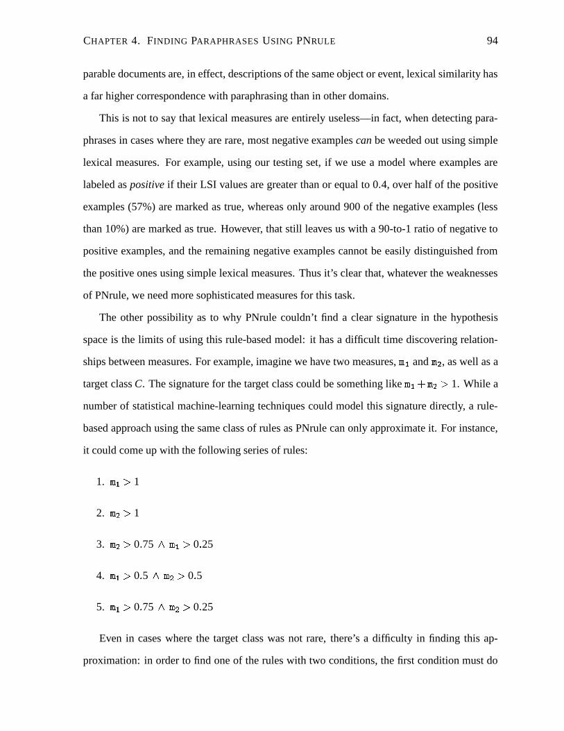
CHAPTER 4. FINDING PARAPHRASES USING PNRULE 94
parable documents are, in effect, descriptions of the same object or event, lexical similarity has
a far higher correspondence with paraphrasing than in other domains.
This is not to say that lexical measures are entirely useless—in fact, when detecting para-
phrases in cases where they are rare, most negative examples can be weeded out using simple
lexical measures. For example, using our testing set, if we use a model where examples are
labeled as positive if their LSI values are greater than or equal to 0 � 4, over half of the positive
examples (57%) are marked as true, whereas only around 900 of the negative examples (less
than 10%) are marked as true. However, that still leaves us with a 90-to-1 ratio of negative to
positive examples, and the remaining negative examples cannot be easily distinguished from
the positive ones using simple lexical measures. Thus it’s clear that, whatever the weaknesses
of PNrule, we need more sophisticated measures for this task.
The other possibility as to why PNrule couldn’t find a clear signature in the hypothesis
space is the limits of using this rule-based model: it has a difficult time discovering relation-
ships between measures. For example, imagine we have two measures, ��� and ��� , as well as a
target class C. The signature for the target class could be something like ��� ����� � 1. While a
number of statistical machine-learning techniques could model this signature directly, a rule-
based approach using the same class of rules as PNrule can only approximate it. For instance,
it could come up with the following series of rules:
1. ��� � 1
2. ��� � 1
3. ��� � 0 � 75 ���� � 0 � 25
4. ��� � 0 � 5 ���� � 0 � 5
5. ��� � 0 � 75 ���� � 0 � 25
Even in cases where the target class was not rare, there’s a difficulty in finding this ap-
proximation: in order to find one of the rules with two conditions, the first condition must do

CHAPTER 4. FINDING PARAPHRASES USING PNRULE 95
better than all other possible first conditions. If, for instance, there was some measure, ��� ,
and ��� � 0 � 3 gave better results than � � � 0 � 75, rule 2 would not be discovered. This problem
arises because the rule-refinement stage uses a greedy search; replacing it with, for example,
a beam search might ameliorate this problem, but there’s no computationally-friendly way to
eliminate it entirely.
In addition, there is another difficulty that is specific to cases in which the target class is
rare. By approximating the signature using several different rules, we split up an already-small
pool of positive examples; each rule will, at best, cover only a tiny number of these examples.
What’s worse, we almost inevitably add error, either because the rules cover examples they
shouldn’t, or because they miss examples.
So, then, we are attempting to detect a semantic relationship with a set of measures that
can at best only approximate semantics, and with a model that, in all likelihood, is only able to
approximate the target-class signature. This, combined with the fact that, when dealing with a
rare target class, even a few errors can lead to terrible results, likely explains why our method
failed. The only question that remains is to what degree each of the two problems contributed
to our method’s failure—a question that will have to be answered in future work.

Chapter 5
Future Work
Clearly, a lot of work still has to be done toward solving this problem. Roughly speaking,
we can separate future work into four groups: preprocessing, method, machine learning, and
measures.
5.1 Preprocessing
One obvious thing to try is to use a partial parser (Abney, 1996, 1997) to split the sentences
in our corpus into clauses, and then attempting to match those clauses. The danger here is
that misparsing sentences might add an unacceptable amount of error; on the other hand, if the
parsing is good, it would reduce noise.
Another preprocessing step that would be worth trying would be to identify any multiword
WordNet entries that might appear in the corpus (e.g., German shepherd. Of course, then one
might want to deal with such multiword entries both as a single unit and as separate words
(since, in theory, a German shepherd could refer to a German who herds sheep).
96

CHAPTER 5. FUTURE WORK 97
5.2 Method
In hindsight, and in particular after reviewing the systems submitted for the RTE challenge, it
has become clear to us that one mistake we have made in our method is to treat an asymmetric
relationship as though it were a symmetric one. Imagine we have two sentences, s1 and s2.
Currently, we use symmetric measures in an attempt to detect whether one sentence contains a
paraphrase of the other. It would be better if instead we dealt with each pair twice: first check
to see if s1 contained a paraphrase of a clause in s2, and then vice versa. This would allow
us to use asymmetric measures: for example, if s1 contains a hypernym of a word in s2, that
increases its chance of containing a paraphrase—however, it does not increase the chance that
s2 contains a paraphrase of a clause in s1, and in fact may decrease that chance. Currently, our
measures cannot reflect that distinction; this change would fix that.
5.3 Machine Learning
As we can see from the submissions to the Pascal RTE challenge, there are a number of po-
tential approaches to the problem of entailment (and thus paraphrasing). Limiting ourselves to
approaches using machine learning, there are several things that could be tried. First, we could
attempt to make changes to PNrule that might improve its performance. For example, we could
try fitness functions other than Z-number or signature clarity. Another idea would be to start
with a pseudo N-stage: this stage would find strong indications that examples were negative,
and then create N-rules accordingly. Why focus on negative examples first? Three reasons:
1. because there’s a large number of negative examples, noise is less likely to be a factor;
2. the strongest indicator that an example is negative is not necessarily the complement of
the strongest indicator that an example is positive; and
3. it’s possible that the strongest indicator that an example is negative in the full data set
will not be the strongest indicator in the set of examples covered by the P-rules.

CHAPTER 5. FUTURE WORK 98
Of course, the pseudo N-stage would be required to keep recall at or near one: the idea would
be to remove obvious negative examples; less obviously labeled examples would be dealt with
in the normal P- and N-stages.
Second, we could adapt a different machine-learning technique to deal with rare classes,
either by redesigning the technique, or by penalizing false negatives much more severely than
false positives. We could pick a method that does not have the weaknesses of a rule-based
system mentioned earlier, or alter PNrule to automatically learn rules that allowed, for example,
attributes to be added together. Alternatively, if we gathered far more data, we might be able
to use something like k-nearest-neighbor unaltered; one advantage of that method is that it can
handle small “clusters” of positive examples surrounded by negative examples within a vector
space.
Finally, related to this second option, we could combine multiple learners, using a method
such as a mixture of experts. These learners could be different machine-learning systems
trained on the same measures, copies of the same machine-learning system trained on dif-
ferent measures, or different systems trained on different measures. We’d want each system
to obtain near-perfect recall, but not necessarily good precision. The idea would be that each
system would cover the same true positives, but different false positives. Assuming this is, in
fact, the case, the combination of systems will outperform the individual systems.
In addition, any future system should be modified to handle negation and numbers; some
of the systems submitted to the Pascal RTE provide ideas as to how this can be done.
5.4 Measures
The Pascal RTE challenge has provided a number of other measures to try; in particular, we feel
that measures based on lexical chains might be helpful, given that this would allows us to add
more contextual information to our measures. Another measure we’d like to try is one based
on latent Dirichlet allocation (Blei et al., 2002), since it is similar in some ways to LSI (which

CHAPTER 5. FUTURE WORK 99
was one of our strongest measures), but may offer some advantages over the former. That said,
given the results of both our and other systems on the Pascal RTE data, it seems as though
paraphrase detection (as well as entailment detection) will require innovative new measures; a
major part of any future work will be finding these measures—for example, using the mutual
information between a noun and and adjective to decide whether that adjective has a large or
small effect on the meaning of the noun phrase (and thus, whether any potential paraphrase will
be more likely to include the adjective). In addition, it would be worthwhile to investigate those
machine learning techniques that incorporate feature selection, since including some measures
does nothing more than introduce noise.
Clearly, there’s still a great deal of work to be done, both on our specific task, and on
detecting entailment in general. We hope that this thesis contributes some ideas to that future
research, as well as perhaps highlighting some pitfalls to avoid.

Bibliography
S. Abney. 1996. Partial parsing via finite-state cascades. Natural Language Engineering,
2(4):337–344.
S. Abney. 1997. The SCOL manual, version 0.1b. http://www.vinartus.net/spa/.
R. Agarwal and M. V. Joshi. 2000. PNrule: A new framework for learning classifier models
in data mining. Technical Report 00-015, Department of Computer Science, University of
Minnesota.
E. Akhmatova. 2005. Textual entailment resolution via atomic propositions. In Proceedings of
the Pattern Analysis, Statistical Modelling, and Computational Learning (PASCAL) Chal-
lenges Workshop on Recognising Textual Entailment.
A. Andreevskaia, Z. Li, and S. Bergler. 2005. Can shallow predicate argument structures
determine entailment? In Proceedings of the Pattern Analysis, Statistical Modelling, and
Computational Learning (PASCAL) Challenges Workshop on Recognising Textual Entail-
ment.
R. Barzilay and N. Elhadad. 2003. Sentence alignment for monolingual comparable corpora. In
Proceedings of the 2003 Conference on Empirical Methods in Natural Language Processing
(EMNLP-03).
R. Barzilay and L. Lee. 2003. Learning to paraphrase: An unsupervised approach using
100

BIBLIOGRAPHY 101
multiple-sequence alignment. In Proceedings of the 2003 Conference of Human Language
Technology/North American Association for Computational Linguistics (HTL/NAACL).
S. Bayer, J. Burger, L. Ferro, J. Henderson, and A. Yeh. 2005. MITRE’s submissions to the
EU Pascal RTE challenge. In Proceedings of the Pattern Analysis, Statistical Modelling,
and Computational Learning (PASCAL) Challenges Workshop on Recognising Textual En-
tailment.
D. Blei, A. Ng, and M. Jordan. 2002. Latent Dirichlet allocation. In T. G. Dietterich, S. Becker,
and Z. Ghahramani, editors, Advances in Neural Information Processing Systems 14, Cam-
bridge, MA. MIT Press.
J. Bos and K. Markert. 2005. Combining shallow and deep NLP methods for recognizing
textual entailment. In Proceedings of the Pattern Analysis, Statistical Modelling, and Com-
putational Learning (PASCAL) Challenges Workshop on Recognising Textual Entailment.
E. Brill. 1994. Some advances in rule-based part of speech tagging. In Proceedings of the
Twelfth National Conference on Artificial Intelligence, p. 722–727, Seattle, WA. American
Association for Artificial Intelligence.
E. Briscoe and J. Carroll. 2002. Robust accurate statistical annotation of general text. In
Proceedings of the Third International Conference on Language Resources and Evaluation,
p. 1499–1504, Las Palmas, Canary Islands, May.
P. Brown, S. A. D. Pietra, V. J. D. Pietra, and R. L. Mercer. 1993. The mathematics of statistical
machine translation. Computational Linguistics, 19(2):263–311.
C. Chen, N. Stoffel, N. Post, C. Basu, D. Bassu, and C. Behrens. 2001. Telcordia LSI engine:
Implementation and scalability issues. In Proceedings of the 11th Int. Workshop on Re-
search Issues in Data Engineering (RIDE 2001): Document Management for Data Intensive
Business and Scientific Applications, p. 51–58, Heidelberg, Germany.

BIBLIOGRAPHY 102
T. Chklovski and P. Pantel. 2004. Verbocean: Mining the web for fine-grained semantic verb
relations. In Proceedings of the Conference on Empirical Methods in Natural Language
Processing (EMNLP-04).
K. Claessen and N. Sorensson. 2003. New techniques that improve mace-style model finding.
In Model Computation - Principles, Algorithms, Applications (Conference on Automated
Deduction (Cade-19) Workshop), Miami, Florida. Cade.
P. Clough. 2001. overlap.pl. http://www.dcs.shef.ac.uk/nlp/meter/
Workshop/overlap.pl.
I. Dagan, O. Glickman, and B. Magnini. 2005. The pascal recognizing textual entailment
challenge. In Proceedings of the Pattern Analysis, Statistical Modelling, and Computational
Learning (PASCAL) Challenges Workshop on Recognising Textual Entailment.
R. de Salvo Braz, R. Girju, V. Punyakanok, D. Roth, and M. Sammons. 2005. An inference
model for semantic entailment in natural language. In Proceedings of the Pattern Analy-
sis, Statistical Modelling, and Computational Learning (PASCAL) Challenges Workshop on
Recognising Textual Entailment.
R. Delmonte, S. Tonelli, M. A. P. Boniforti, A. Bristot, and E. Pianta. 2005. Venses — a
linguistically-based system for semantic evaluation. In Proceedings of the Pattern Analy-
sis, Statistical Modelling, and Computational Learning (PASCAL) Challenges Workshop on
Recognising Textual Entailment.
A. Echihabi, U. Hermjakob, E. Hovy, D. Marcu, E. Melz, and D. Ravichandran. 2003.
Multiple-engine question answering in textmap. In E. Voorhees and L. P. Buckland, edi-
tors, The Twelfth Text REtrieval Conference Proceedings (TREC 2003).
C. Fellbaum, editor. 1998. WordNet: An Electronic Lexical Database. The MIT Press.

BIBLIOGRAPHY 103
A. Fowler, B. Hauser, D. Hodges, I. Niles, A. Novischi, and J. Stephan. 2005. Applying
COGEX to recognize textual entailment. In Proceedings of the Pattern Analysis, Statistical
Modelling, and Computational Learning (PASCAL) Challenges Workshop on Recognising
Textual Entailment.
O. Glickman, I. Dagan, and M. Koppel. 2005. Web based probabilitistic textual entailment.
In Proceedings of the Pattern Analysis, Statistical Modelling, and Computational Learning
(PASCAL) Challenges Workshop on Recognising Textual Entailment.
D. Graff. 2003. English Gigaword. http://www.ldc.upenn.edu/Catalog/
CatalogEntry.jsp?catalogId=LDC2003T05.
V. Hatzivassiloglou, J. L. Klavans, M. L. Holcombe, R. Barzilay, M.-Y. Kan, and K. R. Mc-
Keown. 2001. Simfinder: A flexible clustering tool for summarization. In Workshop on Auto-
matic Summarization, North American Association for Computational Linguistics, Pittsburg
(PA), USA.
V. Hatzivassliloglou, J. Klavans, and E. Eskin. 1999. Detecting text similarity over short pas-
sages: exploring linguistic feature combinations via machine learning. In Proceedings of
Empirical Methods in Natural Language Processing, MD, USA.
J. Herrera, A. Penas, and F. Verdejo. 2005. Textual entailment recognition based on depen-
dency analysis and wordnet. In Proceedings of the Pattern Analysis, Statistical Modelling,
and Computational Learning (PASCAL) Challenges Workshop on Recognising Textual En-
tailment.
G. Hirst and D. St-Onge. 1998. Lexical chains as representation of context for the detection
and correction of malapropisms. In C. Fellbaum, editor, WordNet: An electronic lexical
database. MIT Press.
R. C. Holte, L. E. Acker, and B. W. Porter. 1989. Concept learning and the problem of small

BIBLIOGRAPHY 104
disjuncts. In Proceedings of the Eleventh International Joint Conference on Artificial Intel-
ligence, p. 813–818, Detroit, Michigan.
V. Jijkoun and M. de Rijke. 2005. Recognizing textual entailment using lexical similarity.
In Proceedings of the Pattern Analysis, Statistical Modelling, and Computational Learning
(PASCAL) Challenges Workshop on Recognising Textual Entailment.
M. V. Joshi, R. C. Agarwal, and V. Kumar. 2001. Mining needles in a haystack: classifying
rare classes via two-phase rule induction. SIGMOD Record (Association for Computing
Machinery Special Interest Group on Management of Data), 30(2):91–102.
M. V. Joshi. 2002. Learning Classifier Models for Predicting Rare Phenomena. Ph.D. thesis,
University of Minnesota.
K. Kipper, H. T. Dang, and M. Palmer. 2000. Class-based construction of a verb lexicon. In
Seventeenth National Conference on Artificial Intelligence, Austin, TX. American Associa-
tion for Artificial Intelligence.
R. Kneser and H. Ney. 1995. Improved backing-off for n-gram language modeling. In Pro-
ceedings of the International Conference on Acoustics, Speech, and Signal Processing, p.
181–184.
H. Kuhn. 1955. The hungarian method for the assignment problem. Naval Research Logistics
Quarterly, 2:83–97.
S. Kurohashi and M. Nagao. 1994. A syntactic analysis method of long Japanese sentences
based on the detection of conjunctive structures. Computational Linguistics.
S. Kurohashi and M. Nagao. 1999. Japanese morphological analysis system JUMAN version
3.61 manual. In Japanese.
R. Landis and G. Koch. 1977. The measurement of observer agreement for categorical data.
Biometrics, 133:159–174.

BIBLIOGRAPHY 105
B. Levin. 1993. English Verb Classes and Verb Alternations: A Preliminary Investigation.
University of Chicago Press.
D. D. Lewis. 1999. Reuters-21578 text categorization test collection distribution 1.0. http:
//www.research.att.com/˜lewis.
C.-Y. Lin and E. Hovy. 2004. Automatic evaluation of summaries using n-gram co-occurence
statistics. In Proceedings of the Document Understanding Conference (DUC). National
Institute of Standards and Technology.
D. Lin and P. Pantel. 2001. DIRT: discovery of inference rules from text. In Knowledge
Discovery and Data Mining, p. 323–328.
D. Lin. 1998. An information-theoretic definition of similarity. In Proceedings of the Interna-
tional Conference on Machine Learning.
B. Magnini, S. Romagnoli, A. Vallin, J. Herrera, A. Penas, V. Peinado, F. Verdejo, and
M. de Rijke. 2003. The multiple language question answering track at CLEF. In Work-
ing Notes for the Cross Language Evaluation Forum (CLEF) Workshop, Norway.
L. Marquez. 2000. Machine learning and natural language processing. Technical Report LSI-
00-45-R, Departament de Llenguatges i Sistemes Informatics (LSI), Universitat Politecnica
de Catalunya (UPC), Barcelona, Spain.
W. McCune. 2004. Otter v3.3. www-unix.mcs.anl.gov/AR/otter.
T. M. Mitchell. 1997. Machine Learning. McGraw-Hill.
D. I. Moldovan, C. Clark, S. M. Harabagiu, and S. J. Maiorano. 2003. Cogex: A logic prover
for question answering. In Proceedings of the 2003 Conference of Human Language Tech-
nology/North American Association for Computational Linguistics (HTL/NAACL).

BIBLIOGRAPHY 106
M. Murata, K. Uchimoto, H. Ozaku, and Q. Ma. 1999. Information retrieval based on stochas-
tic models in IREX. In Proceedings of the Information Retrieval and Extraction Exercise
(IREX) Workshop.
E. Newman, N. Stokes, J. Dunnion, and J. Carthy. 2005. UCD IIRG approach to the textual
entailment challenge. In Proceedings of the Pattern Analysis, Statistical Modelling, and
Computational Learning (PASCAL) Challenges Workshop on Recognising Textual Entail-
ment.
F. Och and H. Ney. 2000. Improved statistical alignment models. In Proceedings of the Asso-
ciation for Computational Linguistics, p. 440–447.
F. Och and H. Ney. 2003. A systematic comparison of various statistical alignment models.
Computational Linguistics, 29(1):19–52.
R. Papka, J. Allan, and V. Lavrenko. 1999. UMass approaches to detection and tracking at TDT.
In Proceedings of the Defense Advanced Research Projects Agency Broadcast Workshop.
M. T. Pazienza, M. Pennacchiotti, and F. M. Zanzotto. 2005. Textual entailment as syntactic
graph distance: a rule based and a SVM based approach. In Proceedings of the Pattern Anal-
ysis, Statistical Modelling, and Computational Learning (PASCAL) Challenges Workshop on
Recognising Textual Entailment.
M. Porter. 1980. An algorithm for suffix stripping. Program, 14(3):130–137.
F. Potencier. 2005. Lingua::Stem::Snowball. http://search.cpan.org/˜fabpot/
Lingua-Stem-Snowball-0.93/lib/Lingua/Ste%m/Snowball.pm.
J. Quinlan. 1986. Induction of decision trees. Machine Learning, 1(1):81–106.
J. Quinlan. 1987. Rule induction with statistical data—a comparison with multiple regression.
Journal of the Operational Research Society, 38:347–352.

BIBLIOGRAPHY 107
J. Quinlan. 1993. C4.5: Programs for Machine Learning. Morgan Kaufmann, San Mateo, CA.
C. Quirk, C. Brockett, and W. Dolan. 2004. Monolingual machine translation for paraphrase
generation. In D. Lin and D. Wu, editors, Proceedings of Empirical Methods in Natural
Language Processing (EMNLP) 2004, p. 142–149, Barcelona, Spain, July. Association for
Computational Linguistics.
R. Raina, A. Haghighi, C. Cox, J. Finkel, J. Michels, K. Toutanova, B. MacCartney, M.-C.
de Marneffe, C. D. Manning, and A. Y. Ng. 2005. Robust textual inference using diverse
knowledge sources. In Proceedings of the Pattern Analysis, Statistical Modelling, and Com-
putational Learning (PASCAL) Challenges Workshop on Recognising Textual Entailment.
J. Rennie. 2005. WordNet::QueryData. http://search.cpan.org/˜jrennie/
WordNet-QueryData-1.39/QueryData.pm.
A. Riazanov and A. Voronkov. 2002. The design and implementation of Vampire. AI Commu-
nications, 15(23).
D. Roth and W. Yih. 2002. Probabilistic reasoning for entity and relation recognition. In The
20th International Conference on Computational Linguistics (COLING).
L. K. Schubert and C. H. Hwang. 2000. Episodic logic meets Little Red Riding Hood: A com-
prehensive, natural represntation for language understanding. In L. Iwanska and S. Shapiro,
editors, Natural Language Processing and Knowledge Representation. MIT/AAAI Press.
Y. Shinyama, S. Sekine, K. Sudo, and R. Grishman. 2002. Automatic paraphrase acquisition
from news articles. In Proceedings of the Human Language Technology (HLT) Conference,
San Diego, USA.
Y. Singer and R. Schapire. 1998. Improved boosting algorithms using confidence-rated predic-
tions. In Proceedings of Conference on Learning Theory (COLT).

BIBLIOGRAPHY 108
D. D. Sleator and D. Temperley. 1993. Parsing English with a link grammar. In Third Interna-
tional Workshop on Parsing Technologies.
P. Strazny, editor. 2005. Encyclopedia of Linguistics, volume 1. Fitzroy Dearborn. 2 Vols.
K. Sudo and S. Sekine. 2001. Automatic pattern acquisition for Japanese information extrac-
tion. In Proceedings of the Human Language Technology (HLT) Conference.
K. Uchimoto, M. Murata, H. O. Q. Ma, and H. Isahara. 2000. Named entity extraction based
on a maximum entropy model and transformation rules. In Proceedings of the 38th Annual
Meeting of the Association for Computational Linguistics (ACL), p. 326–335.
S. Vogel, H. Ney, and C. Tillmann. 1996. HMM-based word alignment in stastical translation.
In Proceedings of the Association for Computational Linguistics, p. 836–841.
E. Voorhees. 2004. Overview of the trec 2004 question answering track. In E. Voorhees
and L. P. Buckland, editors, The Thirteenth Text REtrieval Conference Proceedings (TREC
2004).
G. M. Weiss. 1995. Learning with rare cases and small disjuncts. In Proceedings of the Twelfth
Joint International Conference on Artificial Intelligence, p. 558–565.
D. Wu. 2005. Textual entailment recognition based on inversion transduction grammars. In
Proceedings of the Pattern Analysis, Statistical Modelling, and Computational Learning
(PASCAL) Challenges Workshop on Recognising Textual Entailment.
D. Wu and P. Fung. 2005. Inversion transduction grammar constraints for mining parallel
sentences from quasi-comparable corpora. In R. Dale, K.-F. Wong, J. Su, and O. Kwong,
editors, Natural Language Processing - the Second International Joint Conference. Springer,
Jeju Island, Korea.