finding maximal cliques in massive networks by h* …linhong/papers/sigmod10.pdffinding maximal...
TRANSCRIPT

Finding Maximal Cliques in Massive Networks by H*-graph
James ChengSchool of Computer
EngineeringNanyang TechnologicalUniversity, [email protected]
Yiping KeDepartment of Systems
Engineering and EngineeringManagement
The Chinese University ofHong Kong
[email protected] Wai-Chee Fu
Department of ComputerScience and EngineeringThe Chinese University of
Hong [email protected]
Jeffrey Xu YuDepartment of Systems
Engineering and EngineeringManagement
The Chinese University ofHong Kong
Linhong ZhuSchool of Computer
EngineeringNanyang TechnologicalUniversity, Singapore
ABSTRACTMaximal clique enumeration (MCE) is a fundamental problem ingraph theory and has important applications in many areas such associal network analysis and bioinformatics. The problem is exten-sively studied; however, the best existing algorithms require mem-ory space linear in the size of the input graph. This has becomea serious concern in view of the massive volume of today’s fast-growing network graphs. Since MCE requires random access todifferent parts of a large graph, it is difficult to divide the graphinto smaller parts and process one part at a time, because eitherthe result may be incorrect and incomplete, or it incurs huge coston merging the results from different parts. We propose a novelnotion, H∗-graph, which defines the core of a network and ex-tends to encompass the neighborhood of the core for MCE compu-tation. We propose the first external-memory algorithm for MCE(ExtMCE) that uses theH∗-graph to bound the memory usage. Weprove both the correctness and completeness of the result computedby ExtMCE. Extensive experiments verify that ExtMCE efficientlyprocesses large networks that cannot be fit in the memory. We alsoshow that the H∗-graph captures important properties of the net-work; thus, updating the maximal cliques in the H∗-graph retainsthe most essential information, with a low update cost, when it isinfeasible to perform update on the entire network.
Categories and Subject DescriptorsG.2.2 [DISCRETE MATHEMATICS]: Graph Theory—Graph al-gorithms
General TermsAlgorithms, Experimentation, Performance
Permission to make digital or hard copies of all or part of this work forpersonal or classroom use is granted without fee provided that copies arenot made or distributed for profit or commercial advantage and that copiesbear this notice and the full citation on the first page. To copy otherwise, torepublish, to post on servers or to redistribute to lists, requires prior specificpermission and/or a fee.SIGMOD’10, June 6–11, 2010, Indianapolis, Indiana, USA.Copyright 2010 ACM 978-1-4503-0032-2/10/06 ...$10.00.
KeywordsMaximal Clique Enumeration, Massive Networks, Scale-Free Net-works, H*-graph, h-index
1. INTRODUCTIONMaximal clique enumeration (MCE) [2, 7] is a long-standing
problem in graph theory. It is closely related to a number of fun-damental graph problems, such as maximal independent sets (orminimal vertex covers) [28], graph coloring [8], maximal commoninduced subgraphs [19], maximal common edge subgraphs [19],etc. Its significance is not just limited to graph theory but also in nu-merous applications in various real-world networks, such as socialnetwork analysis [15], hierarchy detection through email networks[10], study of structures in behavioral and cognitive networks [3],statistical analysis of financial networks [6], clustering in dynamicnetworks [26], the detection of emergent patterns in terrorist net-works [4], as well as various applications in computational biology[1], protein-protein interaction complex detection [29], and cluster-ing protein sequences [23].
MCE algorithms have been extensively studied [2, 7, 28, 20, 19,21, 26, 1, 27, 9, 12, 25]. The worst-case time complexity of in-memory algorithms have proved to be optimal recently [27]; how-ever, the best existing algorithms require space which is asymptot-ically linear in the size of the input graph. Unfortunately, manyreal-world networks have grown exceedingly large in recent yearsand are continuing to grow at a fast rate. For example, the Webgraph has over 1 trillion webpages (Google), most social networks(e.g., Facebook, MSN) have millions to billions of users, many ci-tation networks (e.g., DBLP, Citeseer) have millions of publica-tions, other networks such as phone-call networks, email networks,stock-market networks, etc., are also massively large.
Despite the low cost of memory, applying in-memory algorithmsis clearly infeasible on such massive data. For large graphs, exter-nal memory algorithms offer a possible recourse; however, design-ing such an algorithm is fraught with difficulties. MCE compu-tations access vertices in a rather arbitrary manner. This poten-tial random disk access requirement makes it difficult to divide thegraph and process it in a part-by-part manner and perhaps suggeststhe reason for the current prevalence in in-memory algorithms fortackling this problem.
447

In this paper, we develop the first external-memory algorithm forMCE (ExtMCE) which operates on the broad class of scale-freegraphs [24, 11]. Extensive studies [14, 24, 6, 5] have shown thatscale-free graphs are prevalent in real-world applications. In partic-ular, Dorogovtsev and Mendesand [11] show that a wide spectrumof real-world networks are scale-free, which include the WWW, ci-tation networks, collaboration networks, neural networks, metabolicreaction networks, genome and protein networks, ecological andfood webs, word web of human language, telephone call graph,mail networks, power grids and industrial networks, electronic cir-cuits, nets of software components, and energy landscape networks.
Given a large input graph G, ExtMCE recursively computes aportion of G at a time, such that each portion can be fit into the mainmemory for MCE computation. Two questions arise: (1) Whatportion of G should be chosen at each recursive step and how? (2)How to ensure that the set of maximal cliques computed locallyat recursive steps is sound and complete with respect to the set ofmaximal cliques globally in G?
To answer the first question, we propose the novel notion of H∗-graph. The key component of the H∗-graph is the largest set of hvertices in G that have degree at least h, called the h-vertices. Thisis inspired by the concept of h-index [16], which is the maximumh for a scientist who has h publications of citations at least h. Theh-index is widely used to assess a scientist’s publication productiv-ity and quality. Putting into the context of a graph, the h-verticescorrespond to the h publications that contribute to the h-index. Theinduced subgraph of G by the h-vertices constitutes the core of theH∗-graph. Then, we extend from this core to their neighborhoodand thus form the H∗-graph.
The H∗-graph is the key component in the first step of ExtMCEand sets the limit on the memory usage for all subsequent steps.To this end, we need to first make sure that the H∗-graph is smallenough to be kept in the memory. For a general graph, the H∗-graph can spread to cover a large part of the graph so that it maybe too large to fit into the memory. However, we show that forscale-free graphs, the H∗-graph is only a small portion of the entiregraph. Furthermore, we derive bounds on the size of the H∗-graphfor scale-free networks, which are also bounds on the memory re-quirement of ExtMCE. We also devise a method to handle the casethat even the H∗-graph cannot be fit into the memory.
Now we answer the second question. MCE computation in-volves random accesses to all parts of G; therefore, if we takeany part of G and compute MCE on each part, then either the setof cliques computed may not be complete and may contain non-maximal ones, or the cost of merging the results from each part andensuring completeness is substantially high.
It is challenging in linking the MCE computation from one partof G to the other parts while ensuring the correctness and com-pleteness of the result. Let Gi be the part of G at the i-th recursivestep of ExtMCE (thus, G1 is the H∗-graph). We formulate Gi insuch a way that it allows smooth transition from Gi to Gi+1 so thatwe can compute a subset of maximal cliques in one part of G, andthen move on to another part until we finish the entire G. We provethat the maximal cliques computed in each local part are indeedmaximal globally in the entire graph. We then prove that the set ofmaximal cliques computed is also complete.
Real-world networks undergo frequent updates. However, thereis only one known algorithm [26] that can be applied to update theset of maximal cliques when a network is updated. Their algorithmis impractical for large networks because the set of maximal cliquesin a large network is too large to be kept in the memory, whilekeeping them on the disk results in extremely high update cost.
We take a new approach. We show that the H∗-graph captures
many important properties of the original network, while the setof maximal cliques computed from the H∗-graph are those thatconsist of the most important vertices in the network. Therefore, wepropose to update only the maximal cliques in the H∗-graph, whichcan be processed in the memory due to the much smaller number.Furthermore, we show that the portion of the updates in G thatare related to the H∗-graph is very small and thus by focusing theupdate maintenance on the H∗-graph, we can significantly reducethe overall update cost. Given the up-to-date H∗-graph, we thenre-compute the whole set of maximal cliques in G on demand.
Finally, we conduct experiments on a set of large real-world net-works, with size up to about 10 million vertices and 80 millionedges, collected from different domains. Our results verify that theH∗-graph represents a significant portion of the original network,and it is effective to use the H∗-graph to bound the memory us-age in ExtMCE. We demonstrate that ExtMCE uses comparabletime, but significantly less memory, as compared with the state-of-the-art in-memory MCE algorithm [27]. When the memory is notsufficient, ExtMCE still computes MCE efficiently with a boundedmemory usage. Our results also verify that our approach of updatemaintenance is effective, and significantly more efficient than [26].
Contributions. We summarize our main contributions as follows.
• We propose ExtMCE, the first external-memory algorithmfor MCE computation. We prove both the correctness andcompleteness of the result computed by ExtMCE.
• We propose the novel notion of the H∗-graph, which is usedto bound the memory usage as well as to guide the recursivesteps of ExtMCE. We derive bounds on the size of the H∗-graph.
• We propose the first feasible solution for update maintenanceof MCE in large networks. We show that by updating themaximal cliques in the H∗-graph, we retain the essential in-formation in the entire network, leading to a low update cost.
Organization. Section 2 formally defines the problem and givesthe basic notations. Section 3 presents the H∗-graph. Section 4details the ExtMCE algorithm. Section 5 discusses update main-tenance. Section 6 reports the experimental results. Section 7 dis-cusses the related work. Section 8 gives the conclusion.
2. PROBLEM DEFINITIONIn this paper, we focus on large graphs whose degree distribu-
tion follows a power law, or called scale-free networks [14, 24].Let G = (V,E) be an undirected and unlabeled graph. We definen = |V | and m = |E|. We define the size of G, denoted as |G|,as |G| = m. Given S ⊆ V , we define the induced subgraph of Gby S as GS = (VS = S,ES = (u, v) : u, v ∈ S, (u, v) ∈ E).We define the set of neighbors of a vertex v in G as nb(v) = u :(u, v) ∈ E, and the degree of v in G as d(v) = |nb(v)|. Simi-larly, we define nb(v,GS) = u : (u, v) ∈ ES and d(v,GS) =|nb(v, GS)|.
A clique in G is a subset of vertices, C ⊆ V , such that theinduced subgraph by C is a complete graph in G. C is called amaximal clique (max-clique for short) in G if there exists no cliqueC′ in G such that C′ ⊃ C.
The problem of Maximal Clique Enumeration (MCE) is: given agraph G, find the set of all maximal cliques in G. In this paper, wesolve the problem of MCE for large scale-free graphs that cannotbe fit in the main memory.
Table 1 shows the notations used frequently in the paper.
448
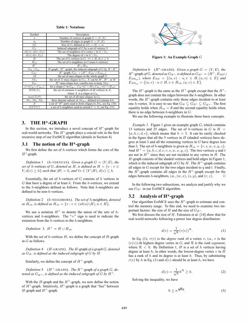
Table 1: Notations
Symbol Descriptionn Number of vertices in graph G = (V,E)m Number of edges in graph G = (V,E)|G| Size of G, defined as |G| = |E| = mGS Induced subgraph of G by a set of vertices S
nb(v); nb(v,GS) The set of neighbors of a vertex v in G / GS
d(v); d(v,GS) The degree of v in G / GS
H The set of h-vertices in G; ∀v ∈ H,d(v) ≥ hHnb The set of h-neighbors in G (non-h-vertices)H+ H ∪Hnb
GH ; GH+ H-graph / H+-graph; the induced subgraph of G by H / H+
GH∗ H∗-graph; GH∗ = (H+, EHH ∪EHHnb)
M the set of max-cliques in the whole graph G
MX the set of X-max-cliques in GX , X can be H∗, H+, or HTH∗ H∗-max-clique tree; a prefix-tree to keep MH∗
C=(CH ∪ CHnb) for a clique C in GH+ : CH=(C ∩H); CHnb
=(C ∩Hnb)HNB(X) the set of common h-neighbors of all vertices in X ,
where X is a clique in GH
maxCL(S) the set of all max-cliques in GS
M1, M2, M3 three disjoint subsets of MH+ , defined in Lemmas 4-6X a set of “H” parts used to form cliques in M3, see Eq. (10)
EXT (C) a set of h-neighbors used to extend C ∈ X , see Eq. (11)
3. THE H*-GRAPHIn this section, we introduce a novel concept of H∗-graph for
real-world networks. The H∗-graph plays a crucial role in the firstrecursive step of our ExtMCE algorithm (details in Section 4).
3.1 The notion of the H*-graphWe first define the set of h-vertices which forms the core of the
H∗-graph.
Definition 1 (h-VERTICES). Given a graph G = (V,E), theset of h-vertices of G, denoted as H , is defined as H = v : v ∈V, d(v) ≥ h such that |H | = h, and ∀v ∈ (V \H), d(v) ≤ h.
Essentially, the set of h-vertices of G consists of h vertices inG that have a degree of at least h. From the h-vertices, we extendto the h-neighbors defined as follows. Note that h-neighbors aredefined to be non-h-vertices.
Definition 2 (h-NEIGHBORS). The set of h-neighbors, denotedas Hnb , is defined as Hnb = v : v ∈ (nb(u)\H), u ∈ H.
We use a notation H+ to denote the union of the sets of h-vertices and h-neighbors. The “+” sign is used to indicate theextension from the h-vertices to the h-neighbors.
Definition 3. H+ = H ∪Hnb .
With the set of h-vertices H , we define the concept of H-graphin G as follows.
Definition 4 (H -GRAPH). TheH-graph of a graph G, denotedas GH , is defined as the induced subgraph of G by H .
Similarly, we define the concept of H+-graph.
Definition 5 (H+-GRAPH). The H+-graph of a graph G, de-noted as GH+ , is defined as the induced subgraph of G by H+.
With the H-graph and the H+-graph, we now define the notionof H∗-graph. Intuitively, H∗-graph is a graph that “lies” betweenH-graph and H+-graph.
a
b c
d e s
w
x y
z
t
q
r
Figure 1: An Example Graph G
Definition 6 (H∗-GRAPH). Given a graph G = (V,E), theH∗-graph of G, denoted asGH∗ , is defined as GH∗ = (H+, EHH∪EHHnb
), where EHH = (u, v) : u, v ∈ H, (u, v) ∈ E andEHHnb
= (u, v) : u ∈ H,v ∈ Hnb, (u, v) ∈ E.
The H∗-graph is the same as the H+-graph except that the H∗-graph does not contain the edges between the h-neighbors. In otherwords, the H∗-graph contains only those edges incident to at leastone h-vertex. It is easy to see that GH ⊆ GH∗ ⊆ GH+ . The firstequality holds when Hnb = ∅ and the second equality holds whenthere is no edge between h-neighbors in G.
We use the following example to illustrate these basic concepts.
Example 1. Figure 1 gives an example graph G, which contains13 vertices and 25 edges. The set of h-vertices in G is H =a, b, c, d, e, which means that h = 5. It can be easily checkedin the figure that all the 5 vertices in H (shaded vertices) have de-gree at least 5 and all the remaining vertices in G have degree lessthan 5. The set of h-neighbors is given as Hnb = r, s, w, x, y, z.And H+ = a, b, c, d, e, r, s, w, x, y, z. The two vertices q and tare not in H+ since they are not incident to any vertex in H . TheH-graph consists of the shaded vertices and bold edges in Figure 1,which is the induced subgraph of G by H . The H+-graph containsall edges in G except for the two edges incident to q and t. Finally,the H∗-graph contains all edges in the H+-graph except for theedges between h-neighbors, i.e., (w, x), (s, y), and (r, z). 2
In the following two subsections, we analyze and justify why weuse GH∗ in our ExtMCE algorithm.
3.2 Analysis of H*-graphOur algorithm ExtMCE uses the H∗-graph to estimate and con-
trol the memory usage. To this end, we need to examine two im-portant factors: the size of H and the size of GH∗ .
We first discuss the size of H . Faloutsos et al. [14] show that forreal-world networks following a power law degree distribution:
d(v) =1
nR(r(v))R. (1)
In Eq. (1), r(v) is the degree rank of a vertex v, i.e., v is the(r(v))-th highest degree vertex in G, and R is the rank exponent,where R < 0. By Definition 1, H is a set of h vertices havingdegree at least h; in other words, the lowest-degree vertex v in Hhas a rank of h and its degree is at least h. Thus, by substitutingr(v) by h in Eq. (1) and d(v) should be at least h, we have
d(v) =1
nRhR ≥ h. (2)
Solving the inequality, we have
h ≤ nR
R−1 . (3)
449

Faloutsos et al. [14] show that R is a constant for most real-world networks, which can be easily measured by plotting the de-gree distribution of the networks. The value of R measured in [14]for three snapshots of the internet graph is between −0.8 and −0.7.For a graph of 1 million vertices, we have h ≤ 464 and therefore|H | ≤ 464 when R = −0.8. The value of h decreases to about300 when R = −0.7. This shows that the number of h-vertices ina large real-world network is small.
Next, we estimate the size of GH∗ . By Eq. (1), we have thefollowing upper bound for |GH∗ |.
|GH∗ | ≤h∑
r=1
(r
n)R. (4)
The right-hand side of Eq. (4) is the sum of degrees of all the h-vertices. Since the edges connecting two h-vertices (if there is any)are counted twice, we have the “<” sign in Eq. (4). The equalityholds when there is no edge connecting two h-vertices; in this case,the H∗-graph consists of h “stars”, each centered at an h-vertex.
We can also obtain a lower bound for |GH∗ | as follows.
|GH∗ | ≥h∑
r=1
(r
n)R −
h(h− 1)
2. (5)
The lower bound occurs when all h-vertices are pairwise con-nected. In this case, all edges connecting two h-vertices are doublecounted and hence deducting the number of these edges from thedegree sum gives the lower bound of |GH∗ |.
Similarly, we also obtain the size of G, which is half of the de-gree sum of all vertices in V , since all edges are counted twice.
|G| =1
2
n∑
r=1
(r
n)R. (6)
By Eq. (4)-(6), we have
2∑h
r=1 rR − nRh(h− 1)∑n
r=1 rR
≤|GH∗ |
|G|≤
2∑h
r=1 rR
∑nr=1 r
R(7)
For a network with R = −0.7 and 1 million vertices, |GH∗ | iswithin [12%, 15%] of the entire network, and the percentage lowersconsiderably when the network becomes larger: the ratio is in therange of [8%, 10%] when n increases to 10 million.
With the result of Eq. (7), the amount of memory required forkeeping GH∗ is reasonable. Another desirable aspect of the H∗-graph is that the rank exponent in Eq. (3) is a constant for most real-world networks. This property allows us to even estimate the size ofGH∗ when the network grows, so that we can predict the memoryresource required at a certain point in the future. For many real-world networks, it is possible to predict the growth of the networkbased on its past growth pattern, and thus we can prepare in advancethe memory resource required for our computation in the future.
3.3 Why H*-graph?We examine why we use GH∗ instead of GH or GH+ . We first
analyze |GH | as follows.
0 ≤ |GH | ≤h(h− 1)
2. (8)
Eq. (8) gives the lower and upper bounds of |GH |. Since his small, if we use GH as the in-memory partition, it leads to too
Algorithm 1 Compute-H∗-graphInput: G = (V,E).Output: The set of h-vertices of G, H , and the set of their neigh-bors, NBH = nb(v) : v ∈ H.
1. Set h← 0 and initialize an empty min-heap, Q;2. Let (d(v), v, nb(v)) be an element in Q, where d(v) is the key;3. Denote the minimum key of Q by min ;4. for each v ∈ V do5. if (h = 0 or (d(v) > h and min > h))6. insert (d(v), v, nb(v)) into Q;7. h++;8. else if (d(v) > h and min = h)9. delete-min and insert (d(v), v, nb(v)) into Q;
10. return H ← v : (d(v), v, nb(v)) ∈ Qand NBH ← nb(v) : (d(v), v, nb(v)) ∈ Q;
many recursive steps in the max-clique computation and hence toomany scans of G from the disk.
As for |GH+ |, let s =∑h
r=1(rn)R, i.e., the degree sum of
h-vertices. |GH+ | reaches its maximum when (1) the number ofh-neighbors is maximized (i.e., |Hnb | = s); (2) the degrees ofh-neighbors rank top among non-h-vertices (i.e., the degree rankof h-neighbors is from (h + 1) to (h + s) in G); and (3) all h-neighbors connect with only vertices in H+ (i.e., all edges incidentto h-neighbors are in GH+ ). Thus, the upper bound of |GH+ | is
|GH+ | ≤1
2(s+
s∑
r=1
(h+ r
n)R)
=1
2
h+s∑
r=1
(r
n)R. (9)
The lower bound of |GH+ | is simply |GH∗ | since GH∗ ⊆ GH+ .Eq. (9) shows that GH+ is too large to be kept in memory. Forexample, when R = −0.7 and n is 1 million, GH+ can be as largeas 65% of the whole graph G.
From the semantic point of view, GH only retains the very coreof G and does not reveal much global information, while GH+ maybe giving too much general information and making it not muchdifferent from G. On the contrary, GH∗ gives the core of G as wellas the relationship from the core to other parts of G. We examineempirically more properties of GH∗ in Section 6.1.
3.4 Computing the H*-graphAlgorithm 1 presents the algorithm for computing the set of h-
vertices H , together with the set of their neighbors NBH . A min-heap Q is used to keep the h-vertices with their neighbors using thevertex degree as the key. Lines 4-9 perform a scan on the verticesin G to check whether a vertex can be added to Q as a potentialh-vertex. A vertex with degree larger than the current h is eitherdirectly inserted to Q in Lines 5-7 (when h can still grow sincethe min-degree in Q is larger than h) or replace the min-degreevertex in Q in Lines 8-9 (if h is incremented, the min-degree vertexno longer satisfies the degree requirement and is thus discarded).Finally, the set of vertices kept in Q is returned as H . After weobtain H and their neighbor sets NBH (i.e., the adjacency lists),we essentially obtain the H∗-graph.
THEOREM 1. Algorithm 1 correctly computes the set of h-verticesof G and the set of their neighbors in O(h log h + n) time andO(|GH∗ |) space, with one scan of G.
PROOF. To prove the correctness, we need to show that: let h0
be the true value of h of G, then the h computed by Algorithm 1
450

is equal to h0. Suppose to the contrary that h < h0, which impliesthat there are h0 > h vertices with a degree greater than h0 >h. However, according to Algorithm 1, these h0 vertices must beinserted into Q at some point, since their degree is greater than hand the value of h is never decreasing in Algorithm 1. Therefore,h computed by Algorithm 1 should be at least h0 in this case. Onthe other hand, h cannot be larger than h0 since each increment ofh (Line 7 of Algorithm 1) follows the definition of h-vertex (Line5). Thus, we have h = h0.
We have O(h) insertions/updates, each takes O(log h) time, plusn comparisons between h and d(v) for each v ∈ V . Space isneeded to keep h-vertices and their adjacency lists, which takesO(|GH∗ |) space. Since each vertex v ∈ V is processed only once,we only need one scan of G.
4. RECURSIVE CLIQUE COMPUTATIONIn this section, we discuss our algorithm ExtMCE. We first give
the framework of ExtMCE as follows.
• The first step: extract GH∗ from G, compute the set of lo-cal max-cliques in GH∗ , obtain and output a subset of globalmax-cliques from local max-cliques by linking to the remain-ing part of G, and update G by removing GH∗ ;
• The i-th step: extract another subgraph Gi (of similar struc-ture as GH∗ ), where |Gi| ≤ |GH∗ |, from G, repeat the firststep (by replacing GH∗ with Gi);The recursive step continues until G becomes empty.
4.1 H*-max-cliques and H*-max-clique treeWe start the first step by defining the notions of H∗-max-cliques
and H∗-max-clique tree.
4.1.1 H*-max-cliquesWe first define the notion of H∗-max-cliques.
Definition 7 (H∗-MAX-CLIQUE). AnH∗-max-clique is a max-clique in GH∗ . The set of all H∗-max-cliques is denoted as MH∗ .
The following lemma states two properties of H∗-max-cliques.
LEMMA 1. The following statements of H∗-max-clique are true:
1. An H∗-max-clique contains at least one h-vertex.
2. An H∗-max-clique contains at most one h-neighbor.
PROOF. Since each h-neighbor in GH∗ is connected to at leastone h-vertex and there is no edge between any two h-neighbors, anH∗-max-clique containing an h-neighbor must also contain at leastan incident h-vertex, which proves the first statement. The secondstatement holds since there is no edge among h-neighbors.
4.1.2 H*-max-clique treeWe now present the data structure used to keep the set of H∗-
max-cliques. Since two cliques may share common vertices, wedefine a prefix-tree structure to represent common vertices in thecliques as common paths.
Definition 8 (H∗-MAX-CLIQUE TREE). GivenGH∗ of a graph,define a total order ≺ on H and Hnb . Moreover, ∀u ∈ H and∀v ∈ Hnb , u ≺ v. The H∗-max-clique tree, TH∗ , of GH∗ is aprefix tree defined as follows.
• The root of TH∗ is λ;
• The children of a vertex in TH∗ are ordered by ≺;
• All vertices in a path in TH∗ are ordered by ≺;
• The set of root-to-leaf paths in TH∗ has a one-to-one corre-spondence to the set of H∗-max-cliques. A root-to-leaf path〈λ, u, . . . , v〉 corresponds to an H∗-max-clique u, . . . , v.
We define ≺ by simply assigning each vertex a unique ID andordering them by their IDs, where the ID of an h-vertex is alwayssmaller than that of an h-neighbor.
By Definition 8, we have the following lemma.
LEMMA 2. The following statements of TH∗ are true:
1. An h-neighbor can only be a leaf in TH∗ .
2. All children of λ are h-vertices.
PROOF. Lemma 1 states that an H∗-max-clique contains at mostone h-neighbor. By the definition of the order ≺ and the tree TH∗ ,an h-neighbor can only be a leaf in TH∗ .
Similarly, all children of λ are h-vertices since an H∗-max-cliquecontains at least one h-vertex as stated in Lemma 1 and all h-vertices are ordered before h-neighbors in a path in TH∗ .
Most existing algorithms for computing max-cliques can be mod-ified to construct TH∗ with small overhead, particularly the algo-rithms [7, 19, 27, 9, 22, 12, 25] that adopt a backtracking searchtree, which is essentially an H∗-max-clique tree. It is not our focusto propose another in-memory MCE algorithm; however, we high-light two improvements that we can make by employing the uniqueproperties of TH∗ .
Given a path p = 〈λ, u, . . . , v〉 in TH∗ , let S be the set of ver-tices that can be used to potentially grow p from v. If S ⊆ Hnb ,we first test if u, . . . , v (the corresponding clique of p), insteadof u, . . . , v, s for some s ∈ S, is maximal. If u, . . . , v is max-imal, by Statement 1 in Lemma 2, we directly create S as the setof children of v (we also mark v for a condition test in Line 7 ofAlgorithm 2). Second, unlike a normal prefix tree or a backtrackingsearch tree, by Statement 2 in Lemma 2, we only need to constructthe subtree rooted at an h-vertex that is a child of λ. These twoimprovements can considerably speed up the process as they savea lot of unnecessary checking and comparisons.
4.1.3 Size estimation of H*-max-clique treeThe first step of our algorithm is critical as it sets the memory
limit for the subsequent recursive steps. In Section 3.2, we givebounds on |GH∗ |. However, there is another element, TH∗ , thatmay take much memory. We estimate |TH∗ | here.
Unlike |GH∗ |, which can be estimated by properties of scale-freenetworks, |TH∗ | is difficult to estimate because the number andsizes of max-cliques in GH∗ vary greatly for different networks.The best known upper bound on the number of max-cliques is ex-ponential [27], which is obviously too loose to be used to estimatethe memory usage.
We devise an estimation strategy that borrows the concept ofKnuth’s method [18] for estimating the size of a backtracking treeT . Let n(T ) be the number of vertices in T . The idea is to ran-domly probe a set of paths P in T and estimate n(T ) = AVGp∈P
(n(p)), where n(p) is the size of a tree with the same root as pand using p as a building path. Let p = 〈v1, v2, . . . , vk〉, n(p) =(1+f1+f1f2+ · · ·+(f1 · · · fk−2fk−1)), where fi is the numberof children of vi. In the simple case that T is a complete binarytree, this method correctly estimates n(T ) as (2k−1). It is shownthat Knuth’s method is unbiased and effective in practice [17].
451

However, Knuth’s method assumes the presence of T so that onecan perform random probing of paths, while TH∗ in our case is notyet constructed when estimating its memory usage. We propose anew method of probing paths in TH∗ by utilizing its unique prop-erties, without actually constructing TH∗ . Each time we randomlychoose a vertex u ∈ H . We consider u as a child of λ and at-tempt to probe randomly a path p from u as follows: we randomlychoose a vertex v from the set of vertices that can be used to po-tentially grow p from u, and then continue the process recursivelyfrom v until the path p cannot be expanded any more (i.e., p cor-responds to an H∗-max-clique). Since the vertices are ordered andnb(v) is available for every v ∈ H , we can virtually probe a patheven though TH∗ does not exist. Thus, we can compute n(p) as wemove along p. Then, we estimate n(TH∗) by averaging n(p) of allthe paths probed.
Our method is simple and yet does not violate the principle ofrandom probing [18]. Our empirical study shows that it gives agood estimation in practice (see Table 5 in Section 6.1).
In the case when memory is very limited such that the availablememory N is smaller than n(TH∗), we remove the lowest-degreevertices from H . The number of vertices to be removed can be ap-proximated as h = (1 −N/n(TH∗))h. Then, we use the remain-ing (h − h) vertices as H and extract a smaller GH∗ accordingly.We re-estimate n(TH∗) for the smaller GH∗ until N > n(TH∗).The memory limit for the subsequent recursive steps is then set tothe size of the smaller GH∗ and the corresponding TH∗ . We maylose some of the nice properties of using GH∗ , especially for dy-namic update maintenance; however, when memory is scarce, thisis a necessary compromise but importantly, our recursive algorithmalso handles the case of limited memory resource.
4.2 From H*-max-cliques to global max-cliquesAn H∗-max-clique C may not be a real max-clique in G; that
is, C is maximal locally in GH∗ but may not be maximal globallyin G. In this subsection, we discuss how we compute global max-cliques from the H∗-max-cliques.
4.2.1 H+-max-cliques: a subset of global max-cliquesWe first define the notion of H+-max-cliques as follows.
Definition 9 (H+-MAX-CLIQUE). AnH+-max-clique is a maxi-clique in GH+ that consists of at least one h-vertex. The set of allH+-max-clique is denoted as MH+ .
LEMMA 3. An H+-max-clique is also a max-clique in G.
PROOF. Proof by contradiction. Let C be an H+-max-cliqueand u be any h-vertex in C. Suppose that C is not maximal in G,i.e., there exists a max-clique C′ in G such that C′ ⊃ C. Then C′
must contain some vertex v, where v /∈ H+ (otherwise C′ mustbe maximal in GH+ and C is not). v /∈ H+ implies that v is notconnected with u, which contradicts that C′ is a clique. Therefore,C must be maximal in G.
With the result of Lemma 3, we have the following theorem.
THEOREM 2. Let M be the set of max-cliques in G. Let M0
be the set of max-cliques in G that consist of at least an h-vertex,i.e., M0 = C : C ∈ M, C ∩H 6= ∅. Then, MH+ = M0.
PROOF. First, Lemma 3 shows that MH+ ⊆ M0. Next, ∀C ∈M0, ∃u ∈ C such that u ∈ H . Since ∀v ∈ C\u, (u, v) ∈ E,we have either v ∈ H or v ∈ Hnb , implying that C ∈ MH+ andhence M0 ⊆ MH+ . Thus, MH+ = M0.
Theorem 2 is important because it enables us to compute a subsetof M separately on a portion of G, output it, and move on to com-puting another subset of M for another portion in the remaining ofG, and so on recursively until we finish the whole graph.
4.2.2 Categorizing H+-max-cliquesIt is infeasible to compute MH+ directly fromGH+ , since GH+
is too large (see Eq. (9) and the analysis right after in Section 3.3).Instead, we compute MH+ from TH∗ . We first define some nota-tion used in the subsequent discussions.
Let MH be the set of all max-cliques in GH . Given a clique Cin GH+ , we define CH = (C∩H) and CHnb
= (C∩Hnb). SinceH+ = (H ∪ Hnb), we have C = (CH ∪ CHnb
). Given a cliqueX in GH , we define the set of common h-neighbors of the verticesin X as HNB(X) = v : v ∈ Hnb ,∀u ∈ X, (u, v) ∈ E.In particular, if C is a path in TH∗ , HNB(CH) defines the set ofh-neighbor leaves sharing the same path CH . Finally, we definemaxCL(S) to be the set of all max-cliques in GS (the inducedsubgraph of G by a set of vertices S).
We first identify three disjoint categories of H+-max-cliques asfollows. Let C = (CH ∪ CHnb
) be an H+-max-clique.
1. “CHnb= ∅”: the set of H+-max-cliques in this category is
defined as M1H+ = C : C ∈ MH+ , CHnb
= ∅.
2. “CHnb6= ∅ and CH ∈ MH”: the set of H+-max-cliques
in this category is defined as M2H+ = C : C ∈ MH+ ,
CHnb6= ∅, CH ∈ MH.
3. “CHnb6= ∅ and CH /∈ MH”: the set of H+-max-cliques
in this category is defined as M3H+ = C : C ∈ MH+ ,
CHnb6= ∅, CH /∈ MH.
Recall that our objective in this subsection is to obtain MH+
from TH∗ or equivalently from MH∗ . Therefore, in the remainingpart of this subsection, we first define three sets of cliques M1,M2, and M3 that can be obtained from MH∗ . We then prove thatM1, M2, and M3 are sound and complete with respect to theabove-defined three categories of H+-max-cliques, respectively.We further prove that M1, M2, and M3 give the complete setof MH+ in Theorem 3. Finally, we show how MH+ can be com-puted from TH∗ in Theorem 4.
We first define M1. Intuitively, M1 contains the max-cliques inMH∗ that are also in MH+ .
LEMMA 4. Let M1 = MH ∩MH∗ . Then, M1 = M1H+ .
PROOF. (Prove M1 ⊆ M1H+ ). Let C be a clique in M1. Since
C ∈ (MH ∩MH∗), C contains only h-vertices and is maximal inGH∗ , which means that the vertices in C do not have any commonh-neighbors (i.e., CHnb
= ∅). Since H+ = (H ∪Hnb), C is alsomaximal in GH+ . Since CHnb
= ∅, we have C ∈ M1H+ .
(Prove M1H+ ⊆ M1). ∀C ∈ M1
H+ , we have CHnb= ∅, which
implies that C = CH and C ∈ MH . We have C ∈ MH∗ as wellsince CHnb
= ∅. Thus, C ∈ (MH ∩MH∗) = M1.
Essentially, each C ∈ M1 corresponds to a root-to-leaf pathin TH∗ where the leaf is an h-vertex. Thus, M1 can be readilyobtained from TH∗ .
We now define M2. Intuitively, for each clique C in M2, its“H” part (i.e., CH ) is in MH ; or equivalently, its “H” part is max-imal in GH .
LEMMA 5. Let M2 = C1 ∪ C2 : C1 ∈ (MH\M1), C2 ∈maxCL(HNB(C1)). Then, M2 = M2
H+ .
452

PROOF. It is obvious that all elements in M2 are cliques by thedefinitions of HNB(·) and maxCL(·).
(Prove M2 ⊆ M2H+ ). ∀C = (C1 ∪ C2) ∈ M2, we have
CH = C1 and CHnb= C2. Since CH ∈ MH , CH is maximal in
GH . Since CHnb∈ maxCL(HNB(CH)), CHnb
is also maximalin GHNB(CH ), which defines the h-neighborhood shared by all ver-tices in CH . Thus, C is maximal in GH+ (i.e., C ∈ MH+). SinceCH /∈ M1, we have HNB(CH) 6= ∅ and thus CHnb
6= ∅. SinceC ∈ MH+ , CH ∈ MH , and CHnb
6= ∅, we have C ∈ M2H+ .
(Prove M2H+ ⊆ M2). ∀C ∈ M2
H+ , CHnb6= ∅ and CH ∈
MH . Thus, CH ∈ (MH\M1). Since C is maximal in H+, CHnb
must be maximal in GHNB(CH), i.e., CHnb∈ maxCL(HNB(CH)).
Let C1 = CH and C2 = CHnb, we have C ∈ M2.
Essentially, the CH of each C ∈ M2 is locally maximal inGH . According to Lemma 5, we can compute M2 as follows.For each path in TH∗ that corresponds to each C1 ∈ MH andhas at least an h-neighbor leaf (since C1 ∈ (MH\M1)), com-pute maxCL(HNB(C1)), and output C = (C1 ∪ C2) for eachC2 ∈ maxCL(HNB(C1)). We will explain how to check whethera path in TH∗ corresponds to a clique in MH later in this section.
Finally, we define M3. Intuitively, for each clique C in M3, its“H” part is no longer maximal in GH but just some proper subsetof a max-clique in GH . The non-maximal “H” part then forms amax-clique in GH+ by taking into account its h-neighborhood.
In order to define M3, we first need to define two notations: Xand EXT (·). We enumerate the proper subsets of a max-clique inMH that have at least one common h-neighbor as
X = C1 : C1 ⊂ C,C ∈ MH , C1 6= ∅,HNB(C1) 6= ∅, and∄C′
1⊆ C′, C′∈ MH , s.t. C1⊂ C′1,HNB(C1)=HNB(C′
1). (10)
The last condition ensures that each C1 ∈ X is not subsumedby its proper superset when forming a clique with its h-neighbors.Then, for each C1 ∈ X , we use EXT (C1) to denote the set ofh-neighbors that can be used to extend C1, defined as
EXT (C1) = C2 : C2 ∈ maxCL(HNB(C1)), and∄C′ ∈ M2, s.t. C′ ⊃ (C1 ∪ C2), and∄C′′
1 ∈ X , s.t. C′′1 ⊃ C1, C2 ∈ EXT (C′′
1 ). (11)
The last two conditions are for the maximality checking of (C1∪C2) in M2 and X , respectively.
LEMMA 6. Let M3 = C1∪C2 : C1 ∈ X , C2 ∈ EXT (C1).Then, M3 = M3
H+ .
PROOF. By the definitions of X and EXT (C1), an elementC ∈ M3 must be a clique.
(Prove M3 ⊆ M3H+ ). We first prove M3 ⊆ MH+ by contra-
diction. Suppose ∃C = (C1 ∪ C2) ∈ M3 such that C /∈ MH+ ,i.e., ∃C′ = (C′
H ∪ C′Hnb
) ∈ MH+ such that C′ ⊃ C. We haveC′
H ⊇ CH = C1 and C′Hnb
⊇ CHnb= C2. Assume that C′
H =CH , then C′
Hnb= CHnb
since CHnbis maximal in GHNB(CH)(=
GHNB(C′
H)) as defined in EXT (CH). This leads to a contradic-
tion of C′ = C to C′ ⊃ C. Thus, C′H ⊃ CH , which implies that
HNB(C′H) ⊆ HNB(CH). Since C′
Hnb⊇ CHnb
and they are max-imal respectively in GHNB(C′
H) and GHNB(CH), but HNB(C′
H) ⊆
HNB(CH), we have C′Hnb
= CHnband HNB(C′
H) = HNB(CH).Since C′
H ⊃ CH and HNB(C′H) = HNB(CH), we have C′
H /∈X (otherwise, CH /∈ X since CH is subsumed by C′
H). There-fore, C′
H can only be in MH . Since C′Hnb
= CHnb6= ∅, we have
C′ ∈ M2. This contradicts to CHnb∈ EXT (CH) since there
exists C′ ∈ M2 such that C′H ⊃ CH and C′
Hnb= CHnb
. Thus,M3 ⊆ MH+ . Finally, ∀C ∈ M3, we have CHnb
6= ∅ since∅ /∈ EXT (CH), and CH /∈ MH since CH ∈ X and is a propersubset of some C′′ ∈ MH . Thus, we further have M3 ⊆ M3
H+ .(Prove M3
H+ ⊆ M3). ∀C ∈ M3H+ , CH /∈ MH and CHnb
6=∅. First, CH must be a proper subset of some C′ ∈ MH . Assumethat CH /∈ X , then CH must be subsumed by some element in X ,contradicting to the maximality of C. Thus, CH ∈ X . We furtherhave CHnb
∈ EXT (CH) since CHnbis maximal in GHNB(CH)
and the maximality of C must be ensured. Thus, C ∈ M3.
Essentially, each C ∈ M3 differs from a clique in M1 or M2 inthat CH is not maximal in GH . This category of H+-max-cliquesis not as straightforward to compute as the first two categories. Wediscuss the details in Section 4.2.3.
We state the completeness and soundness of (M1 ∪M2 ∪M3)with respect to the whole set MH+ in the following theorem.
THEOREM 3. MH+ = (M1 ∪ M2 ∪ M3), where M1, M2
and M3 are defined in Lemmas 4-6.
PROOF. By the categorization, M1H+ , M2
H+ and M3H+ are
disjoint and (M1H+ ∪ M2
H+ ∪ M3H+) gives exactly MH+ . By
Lemmas 4-6, we have (M1 ∪M2 ∪M3) = MH+ .
Now we show that TH∗ (plus the knowledge of the edges be-tween the h-neighbors) is sufficient to compute MH+ . We onlyneed partial GHnb
but do not keep GHnbin memory (see details in
Section 4.2.3). Before discussing the computation of MH+ fromTH∗ , we first show that MH can be obtained from TH∗ by thefollowing lemma.
LEMMA 7. ∀C ∈ MH , there exists a path p ∈ TH∗ such thatthe set of h-vertices in p equals to C.
PROOF. For each C ∈ MH , we sort the vertices in C by ≺as C = v1, . . . , vk. First, if HNB(C) = ∅, since C is max-imal in GH , there must exist a root-to-leaf path p = 〈v1, . . . vk〉in TH∗ . Next, if HNB(C) 6= ∅, i.e., ∃u ∈ HNB(C), thenp = 〈v1, . . . , vk, u〉 must be a root-to-leaf path in TH∗ (since Cis maximal in GH).
THEOREM 4. MH+ can be computed from TH∗ and GHnb.
PROOF. By Lemma 7, every C ∈ MH exists in TH∗ . There-fore, MH can be computed from TH∗ by removing all h-neighborleaves and checking the maximality of all remaining paths (Thiscan be incorporated into the maximality checking when construct-ing TH∗ without any extra cost). Thus, ∀C ∈ MH+ , CH canbe obtained from TH∗ . On the other hand, the set of common h-neighbors, HNB(CH), can be obtained from the h-neighbor leavesin TH∗ , from which the corresponding CHnb
can be computed if weknow the part of GHnb
that gives GHNB(CH).
Example 2. Figure 2 gives the H∗-max-clique tree TH∗ (withh-vertices shaded) computed from the GH∗ of the example graphG in Figure 1. Each root-to-leaf path in TH∗ represents an H∗-max-clique and thus there are totally eight H∗-max-cliques. TheMH consists of only two cliques a, b, c and b, c, d, e (MH =abc, bcde for short), which can be obtained from TH∗ too.
The set of H+-max-cliques obtained from the GH+ in Figure1 is MH+ = abcwx , acy , bcde, cey , drz , esy. We now com-pute M1, M2, and M3 from TH∗ (and partial GHnb
). First, byLemma 4, M1 = (MH ∩ MH∗) = bcde, which is the onlyroot-to-leaf path in TH∗ with a non-h-neighbor leaf. Next, byLemma 5, we have (MH\M1) = abc. Therefore, the C1 in
453

Figure 2: TH∗ of G in Figure 1
M2 can only be abc. Then HNB(abc) = w, x, which are thecommon h-neighbor leaves of paths in TH∗ containing abc. Sincew and x are connected in G, we have maxCL(HNB(abc)) =wx. And thus M2 = abcwx. Finally for M3, we haveX = ac, ce, d, e. Essentially we should enumerate all propersubsets of a clique in MH . However, many of them are subsumedby their proper supersets in X or MH . For example, a is subsumedby ac since HNB(a) = HNB(ac) = w, x, y. Then for eachC1 ∈ X , we compute EXT (C1). For example, considering ac,maxCL(HNB(ac)) = wx, y but EXT (ac) = y. Note thatwx ∈ maxCL(HNB(ac)) is excluded from EXT (ac) becauseacwx is checked to be non-maximal wrt. abcwx ∈ M2. Similarly,we have EXT (ce) = y, EXT (d) = rz, and EXT (e) =sy. Thus, by Lemma 6, M3 = acy, cey, drz, esy. It is easyto see that (M1 ∪M2 ∪M3) gives exactly MH+ . 2
4.2.3 Computing H+-max-cliques from H*-max-cliquesWe now discuss the algorithm to compute M1, M2 and M3, as
shown in Algorithm 2.It is straightforward to obtain both M1 and M2, by performing
a depth-first search (DFS) on TH∗ (Lines 2-9). We do not storeexplicitly the set MH and search it to check whether C1 ∈ MH
(Line 7). Instead, we mark each vertex u whose root-to-u pathforms a clique in MH when we construct TH∗ (see the last para-graph of Section 4.1.2). Thus, we only need to check whether vk−1
is marked in Line 7. We explain how to compute maxCL(·) later.To obtain M3, we first compute X in Line 10 as follows. We
enumerate all proper subsets of each C1 ∈ MH in Line 7. Wethen check the conditions defined in X (see Eq. (10)) to prunethe unqualified subsets. The checking of the last condition in X issimilar to the maximality checking when constructing TH∗ . Notethat the set HNB(C) of a clique C can be easily obtained fromTH∗ as the set of h-neighbor leaves of the paths containing C.
Given X , we then compute EXT (C′1) for each C′
1 ∈ X (Line12). The maximality checking defined in EXT (C′
1) (see Eq. (11))is done in the same way as that in X . As for the computation ofmaxCL(HNB(C′
1)), we use an existing in-memory MCE algo-rithm. Since HNB(C′
1) consists of common h-neighbors of allvertices in C′
1, HNB(C′1) is small and thus it is efficient to com-
pute maxCL(HNB(C′1)).
However, in order to compute maxCL(HNB(C′1)), we need to
know the induced subgraph GHNB(C′
1). Note that once we get TH∗ ,
we remove GH∗ from the memory. Thus, we now have more spaceto keep partial GHnb
. In order to avoid random access to G in thedisk, we do the following. Let N be the available memory. For allh-neighbor leaves in TH∗ ordered by the DFS traversal, we dividethem into k partitions Pi (1 ≤ i ≤ k) such that the adjacency listsof the h-neighbors in each Pi can fit into N . We then read G fromthe disk sequentially and for each v ∈ Hnb, we write (nb(v)\H)into the partition(s) v is in. We keep the first partition in the mem-ory, while each of the other partitions is written into consecutivedisk pages. In this way, we read a partition (partial GHnb
) into
Algorithm 2 Compute-H+-max-cliquesInput: TH∗ (and partial GHnb
)Output: MH+
1. InitilizeM1 =M2 =M3 = ∅;2. for each path p = 〈v1, . . . , vk〉 in TH∗ do3. if (vk ∈ H)4. M1 ←M1 ∪ (v1, . . . , vk); /∗ by Lemma 4 ∗/5. else6. C1 ← (v1, . . . , vk−1);7. if (C1 ∈ MH ) /∗ by Lemma 5 ∗/8. Compute maxCL(children(vk−1));9. M2 ←M2∪C1 ∪ C2 : C2 ∈ maxCL(children(vk−1));
10. Compute X ; /∗ see Eq. (10) ∗/11. for each C′
1 ∈ X do /∗ by Lemma 6 ∗/12. Compute EXT (C′
1); /∗ see Eq. (11) ∗/13. M3 ←M3 ∪ C′
1 ∪ C′2 : C′
2 ∈ EXT (C′1);
14. returnMH+ ← (M1 ∪M2 ∪M3);
the memory each time when computing maxCL(HNB(C′1)) and
avoid random access in the disk.
4.3 Recursive stepsNow, MH+ is computed and outputted, and GH∗ and TH∗ are
discarded. We are ready to move on to the remaining part of G.Let G′ be the remaining part of G after removing GH∗ , which
means that we delete all h-vertices and their incident edges fromG to give G′. The first step is to extract a subgraph of G′ thatwe can compute the max-cliques from it in the memory. Can weextract another H∗-graph G′
H∗ from G′ (wrt. another h′) in thesame way as we extract GH∗ from G? For any vertex v in G′,d(v) ≤ h (otherwise v should be in GH∗ instead). Thus, h′ ≤ hand |G′
H∗ | ≤ h2. In this case, G′H∗ is too small and we will need
to scan G many times to compute M, which is not desirable.We propose to extract a subgraph from G′ with a similar size to
GH∗ as follows.
Definition 10 (L∗-GRAPH). Let L be a set of vertices ran-domly selected from G′ = (V ′, E′) such that
∑
v∈L
d(v,G′) ≃ |GH∗ |. (12)
We define GL∗ = (L ∪ Lnb , ELL ∪ ELLnb), where Lnb = v :
u ∈ L, v /∈ L, (u, v) ∈ E′, ELL = (u, v) : u, v ∈ L, (u, v) ∈E′, and ELLnb
= (u, v) : u ∈ L, v ∈ Lnb , (u, v) ∈ E′.
Note that GL∗ is defined based on L in the same way as GH∗
is on H . Therefore, we can apply the method developed for GH∗
in Sections 4.1 and 4.2 to compute the max-cliques from GL∗ , bysimply replacing H with L. After that, G′ is updated by removingGL∗ . This process continues recursively until G′ becomes empty.
There is a small problem in the transition from H to L. Considerthe 2nd recursive step, i.e., the step right after we compute MH+ .A clique C may be maximal in GL+ , but C may not be maximal inG, because it is possible that ∃C′ ∈ MH+ such that C′ ⊃ C andC′
Hnb= C. We remark that if C is maximal in GH+ , then C is
also maximal in G, because H only has connection with Hnb whileL may have connection with both H and Lnb .
We address this problem as follows. For each C ∈ MH+ , if|CHnb
| > 1, we keep CHnbin a hashtable. Let C′ be a max-clique
in GL+ . If |C′| = 1, then C′ = v is maximal in G only ifd(v) = 0. If |C′| > 1, we hash C′ to check if C′ exists in thehashtable. If C′ is not in the hashtable, then C′ is maximal in Gand we also add C′
Lnb(if |C′
Lnb| > 1) into the hashtable for the
454

Algorithm 3 ExtMCEInput: G, recursive depth k, size bound bOutput: M
1. if (G is empty) return;2. if (k = 1) /∗ 1st-step: compute GH∗ ∗/3. Compute-H∗-graph (Alg. 1);4. else /∗ recursive steps: compute GL∗ ∗/5. Compute-L∗-graph with size bounded by b (Def. 10);6. Construct TH∗ (or TL∗ ) by an existing MCE algorithm A;7. Compute-H+(or L+)-max-cliques (Alg. 2);8. if (k = 1) /∗H+-max-cliques are max-cliques by Theorem 2 ∗/9. Build a global hashtable X (see the last paragraph of Section 4.3);
10. Output H+-max-cliques;11. else12. Check the maximality of L+-max-cliques by X;13. Output L+-max-cliques that are globally maximal;14. Update X (see the last paragraph of Section 4.3);15. Remove GH∗ (or GL∗ ) from G;16. ExtMCE(G, k + 1, |GH∗ |);
maximality checking in subsequent recursive steps. Otherwise, C′
is not maximal and we also remove C′ from the hashtable, sinceC′ will not be computed again in subsequent steps. We also controlthe number of cliques kept in the hashtable as follows. After eachround of max-clique computation from GL∗ , we delete all C inthe hashtable if ∃v ∈ C such that v ∈ L, because all max-cliquescontaining v are generated after we finish GL∗ (by Theorem 2).
4.4 Overall Algorithm: ExtMCEThe overall recursive algorithm ExtMCE is presented in Algo-
rithm 3. The set of all max-cliques in G can be computed by in-voking ExtMCE(G, 1, 0). The second parameter k of the algorithmspecifies the depth of the recursive process and the last parameterb sets a size bound on the portion of G that is under max-cliquecomputation in each recursive step. b is set as 0 initially for the firststep and as |GH∗ | for the following recursive steps.
We state the correctness of ExtMCE in the following theorem.
THEOREM 5. The results returned by ExtMCE is sound andcomplete with respect to the set of all max-cliques in G.
PROOF. We first prove the soundness. At the first recursive step,the set of H+-max-cliques is computed in Line 7 and outputteddirectly in Line 10 of ExtMCE. The H+-max-cliques are proved tobe maximal in G in Theorem 2. Next, at each subsequent recursivestep, L+-max-cliques are computed (Line 7). The maximality ofthe outputted L+-max-cliques is ensured by the checking in Line12 of ExtMCE.
We now prove the completeness. At the first step, the set ofH+-max-cliques is complete with respect to the max-cliques inG that contain at least one vertex in H (by Theorem 2). At thesecond recursive step, L+-max-cliques are computed in the sameway as H+-max-cliques (Line 7). This means that the set of L+-max-cliques is complete with respect to the set of max-cliques in(G\GH∗) that contain at least one vertex in L. Combining withthe H+-max-cliques (computed from GH∗) that contain at leastone vertex in L, it gives a complete set of max-cliques in G thatcontain at least one vertex in L. Similarly by recursion, a com-plete set of max-cliques in G that contain at least one vertex in thecorresponding L is given after each recursive step. Since the recur-sion terminates when the graph G becomes empty (i.e., all verticeshave been considered to form max-cliques), the algorithm gives acomplete set of max-cliques in G.
Complexity. The memory space complexity of ExtMCE is O(|GH∗ |
+|TH∗ |). We need O(|G|/|GH∗ |) scans of G for the entire pro-cess. We now analyze the time complexity of ExtMCE when com-pared with an in-memory MCE algorithm A. Let A(G) denote thealgorithm A when it is applied directly to the whole graph G. If weonly consider the in-memory operations, the time required for theentire recursive steps in ExtMCE is comparable to that of A(G).This is because Algorithm 2 essentially expands those paths inTH∗ (or TL∗ ) that would be generated by A(G) as well, while thecomputation of each maxCL(HNB(·)) is also necessary in A(G).Thus, if the memory is big enough to hold the whole graph G,ExtMCE performs comparably to A(G). However, if the mem-ory is insufficient (a typical case for a massive graph G), A(G)would incur many random disk accesses to G, while ExtMCE hasa bounded number of scans of G, which is much more efficient.These conclusions are empirically verified by our experiments.
5. UPDATE IN DYNAMIC NETWORKSWe consider two types of updates: edge insertion and edge dele-
tion. Vertex insertion/deletion can be considered as a series of edgeinsertions/deletions proceded/followed by the insertion/deletion ofan isolated vertex, which is a rather trivial operation. Note that Gis also updated, but we focus our discussion on updates directly re-lated to the H∗-max-cliques. In other words, we only maintain theH∗-max-cliques to be up-to-date, while we compute the set of allmax-cliques M periodically or on demand.
We first consider the insertion of a new edge e = (u, v) and thepossible updates to H∗-max-cliques. First, if u, v /∈ H , we donot need to update H or TH∗ , unless u and/or v now becomes anh-vertex. Next, if u ∈ H and/or v ∈ H , inserting e creates newH∗-max-clique(s). Let NBuv = nb(u) ∩ nb(v) denote the set ofcommon neighbors of u and v. We find the cliques that can formlarger cliques with u, v as S = C : C ⊆ (C′ ∩ NBuv ), C
′ ∈MH∗ , C 6= ∅, which can be obtained easily by traversing TH∗ .To ensure the maximality, we take away non-maximal cliques in Sand get SM = C : C ∈ S ,∄C′ ∈ S s.t. C′ ⊃ C. Then, foreach C ∈ SM , we insert (C ∪ u, v) into TH∗ . We also remove(C ∪ u) and/or (C ∪ v) from TH∗ if they are originally in thetree. Note that if S = ∅, then u, v is maximal and we simplyinsert u, v into TH∗ .
We now consider deleting an edge e = (u, v). If u, v /∈ H , thereis no update needed for H and TH∗ . If u ∈ H and/or v ∈ H , weneed to remove from TH∗ all H∗-max-cliques containing both uand v. Thus, we need to find S ′ = C : u, v ∈ C,C ∈ MH∗.Assume that u ≺ v, we can obtain S ′ by finding all occurrences ofv in the subtree rooted at each occurrence of u in TH∗ , and collect-ing the H∗-max-cliques containing both u and v by traversing thecorresponding paths. We remove each C ∈ S ′ from TH∗ . We alsoinsert (C\u) and/or (C\v) if they now become maximal.
We give an analysis on the cost of the updates as well as on thefrequency of the updates.
On edge insertion, the cost is O(|TH∗ |+ |S|2 +∑
C∈SM(|C ∪
u, v| log favg)) time, where favg is the average number of chil-dren of a node in TH∗ . Computing S takes O(|TH∗ |) time. Com-puting SM takes time less than |S|2 since we do not need to com-pare cliques with the same size, or those largest cliques in S . Inmost cases, |S| is small because otherwise it implies that u andv are very closely related and hence the edge (u, v) is likely toalready exist. Finally, inserting each (C ∪ u, v) takes at mostO(log favg) time at each level of TH∗ . On edge deletion, it takesO(|TH∗ |+
∑C∈S′(|C| log favg)) time to obtain S ′ and delete C
(as well as to insert (C\u) and/or (C\v) if they are maximal).Now we examine how frequent these updates are performed.
Since we only perform updates related to theH∗-max-cliques, there
455

is no update for the insertion or deletion of an edge (u, v), whereu, v /∈ H . As shown in Section 3.2, the size of H , i.e., h, is usuallyvery small compared to the total number of vertices in G. There-fore, the percentage of the updates in G that can “hit” an h-vertexand thus trigger an update in H∗-max-cliques is very low, which isalso verified in our experimental studies.
6. EXPERIMENTAL EVALUATIONWe evaluate the performance of our method, comparing with the
state-of-the-art in-memory MCE algorithm [27] and the only exist-ing streaming MCE algorithm for dynamic networks [26], denotedas in-mem and streaming in our experiments. We ran all experi-ments on a machine with a 3.0GHz Pentium 4 CPU and 2GB RAM,running Windows XP.Datasets. We use four datasets: protein, blogs, LiveJournal (LJ),and Web. Protein is a human protein interaction network fromthe Human Protein Database (www.hprd.org), in which verticesare proteins and edges are protein-protein interactions. The blogsnetwork is collected from the top-15 popular queries published byTechnorati (technorati.com) every three hours from Nov 2006 toMar 2008. In the blogs network, vertices are blogs and edges in-dicate that two blogs appear in the same search result. LJ is thefree on-line community called Livejournal (www.livejournal.com),where vertices are members and edges represent friendship betweenmembers. The Web graph is obtained from the YAHOO webspamdataset (barcelona.research.yahoo.net/webspam), where vertices arepages and edges are hyperlinks. We give the details of each dataset(number of vertices and edges, physical storage size) as follows.
Table 2: Datasets (K = 1,000 and M = 1,000,000)protein blogs LJ Web
n = |V | 20K 1M 4.8M 10Mm = |E| 40K 6.5M 43M 80MStorage size (MB) 1 186 1310 2613
6.1 Evaluation of the H*-graphTable 3 shows that it is very efficient to extract GH∗ from G.
The majority of the time is used to read the graph from the disk,which is an inevitable cost.
Table 3: Time and memory usage of extracting GH∗
protein blogs LJ WebTotal time (sec) 0.3 38 243 524Disk-read time (sec) 0.2 31 199 405Memory (MB) 1.2 8.5 27 140
Table 4 reports the sizes of H , Hnb , GH , GH∗ and GH+ . Wealso give a better perception on the sizes of GH , GH∗ and GH+ astheir ratio to G (given in parenthese in the table). For all datasets,H is small but it extends to a much larger h-neighbor set Hnb .As a result, GH is too small, thus requiring many disk scans forMCE computation, while GH+ is too large, thus demanding toomuch memory. On the contrary, GH∗ is much smaller than GH+
but is significantly greater than GH , thus allowing more efficientMCE computation with reasonable memory usage. As seen fromthe size ratio, LJ has a relatively smaller GH∗ and GH+ than otherdatasets, which is mainly because the vertices in LJ are less denselyconnected as indicated by its small |H | wrt. |V |.
Table 4: Sizes of H , Hnb , GH , GH∗ and GH+
protein blogs LJ Web|H| 77 718 987 2982|Hnb | 4K 192K 441K 4.4M|GH | 0.5K (1%) 37K (0.6%) 25K (0.06%) 29K (0.04%)|GH∗ | 8.6K (22%) 840K (13%) 1.7M (4%) 25M (31%)|GH+ | 21K (54%) 4M (64%) 11M (25%) 54M (68%)
Table 5 shows the average closeness of the h-vertices, the per-centage of vertices in G that are reachable from the h-vertices(reachability), the number of max-cliques, and the accuracy of es-timating |TH∗ |. The closeness of an h-vertex u is defined asAVGv∈V,dist(u,v)6=∞(dist(u, v)), where dist(u, v) is the lengthof the shortest path from u to v in G.
Table 5: Closeness, reachability, # of max-cliques, and |TH∗ |protein blogs LJ Web
closeness (h-vertices) 3.1 3.4 4.3 7.1reachability (h-vertices) 47% 56% 100% 73%# of max-cliques 25K 1.1M 173M 267M(contain h-vertices) 239 4K 69K 7.8M(contain h-neighbors) 12K 510K 43M 146M(estimated |TH∗ |)/|TH∗ | 1.00 1.01 0.93 0.97
The closeness shows that from the h-vertices, we can reach othervertices in G within a few steps and we are able to reach the ma-jority of the vertices in G. This result demonstrates that GH∗ rep-resents a significant portion of G and that GH∗ also has a closerelationship with the rest part of G.
Table 5 also reports the number of all max-cliques, the numberof those max-cliques containing h-vertices and h-neighbors. Theresult shows that the number of max-cliques containing h-verticesis significantly smaller than that of all max-cliques. The result jus-tifies the feasibility of our update maintenance based on a muchsmaller set of cliques containing h-vertices since it is much moreefficient. From the h-vertices we can extend to the h-neighbors,while the result shows that the set of max-cliques containing h-neighbors represents a large portion of the whole set of max-cliques.
Finally, Table 5 shows that our method of estimating |TH∗ | ishighly accurate. Thus, the result verifies the effectiveness of settingmemory-bound at the first step of ExtMCE.
6.2 Performance of ExtMCEFigure 3 reports the total running time and peak memory con-
sumption of finding the set of all max-cliques using ExtMCE, in-mem, and streaming, respectively.
First, on the smaller networks protein and blogs, ExtMCE is asfast as in-mem, but with only 1 quarter of the memory usage ofin-mem. The result verifies our assertion in Section 4.4 that thetime complexity of ExtMCE is indeed comparable to that of an in-memory MCE algorithm.
On the larger networks, the advantage of ExtMCE over in-memis immediately seen. As shown in Figure 3(b), in-mem runs out ofmemory, while ExtMCE computes the result for all the networkswith a bounded memory consumption. The corresponding runningtime for in-mem is thus not shown in Figure 3(a) since in-mem doesnot complete the MCE task.
We are only able to obtain the result of streaming for the small-est protein network, which already takes many orders of magnitudemore time to complete. The result is because streaming reads an
456

1
10
100
1k
10k
100k
protein blogs LJ Web
Run
ning
tim
e (s
ec)
ExtMCEin-mem
streaming
(a) Running Time
0
500
1000
1500
2000
2500
protein blogs LJ Web
Mem
ory
usag
e (M
B)
ExtMCEin-mem
streaming
(b) Memory Consumption
Figure 3: Performance of ExtMCE
edge at a time and updates the current set of max-cliques for eachedge. We report this result to demonstrate that although streamingreads the graph only once, the time complexity of such a streamingalgorithm for MCE computation is extremely high. On the con-trary, ExtMCE reads the graph O(|G|/|GH∗ |) times, but is able tocompute MCE efficiently with bounded memory usage.
We further analyze ExtMCE by showing the number of recur-sions it requires for each dataset. As shown in Table 6, the numberof recursions actually performed by ExtMCE is very close to the es-timated number, |G|/|GH∗ |. LJ has a higher number of recursionssince its H∗-graph is relatively smaller as shown in Table 4.
Table 6: Actual/estimated number of recursionsprotein blogs LJ Web
# of recursions 5 9 25 7|G|/|GH∗ | 4.5 7.7 24.6 3.2Time (1st recursion) 67% 36% 2% 34%
Table 6 also shows that the percentage of the total running timeused for the first recursive step, i.e., ExtMCE operates on GH∗ . Itshows that a large portion of the time is spent on computing themax-cliques at the first step (except LJ), which also justifies thechoice of GH∗ for dynamic update maintenance. We also find thatthe peak memory consumption indeed occurs at the first recursivestep, which verifies the correctness of O(|GH∗ | + |TH∗ |) as thememory bound for ExtMCE.
6.3 Performance on Update MaintenanceTable 7 reports the results for update maintenance. We use the
blogs network, whose edges are associated with a timestamp, span-ning over 12 months. We average the results for every two month-period, shown as P1-P6 in Table 7. The network grows from 347Kedges to 6.5M edges.
Table 7 shows that the average time of processing an edge inser-tion that triggers an update in TH∗ , shown as “Avg. update time”,is only 2 to 3 msec. The exception is P1 which requires 10 msec.This is because the initial network is not large enough and henceTH∗ changes considerably during P1, which is also reflected bythe rapid increase in the number of h-vertices from P1 to P2.
Table 7 also shows “# of updates in GH∗”, which is the numberof edge insertions that trigger an update in TH∗ , and “# of updatesin G”, which is the number of all edges inserted into the network.On average, the percentage of edges that trigger an update in TH∗
is only 3.8%, which is a small portion of the total updates. Thus,updating only TH∗ is a feasible solution to handle frequent updates.
Among the existing algorithms, streaming is the only one thatupdates the set of max-cliques upon each edge insertion. However,streaming is three orders of magnitude slower than our algorithmon average. We do not report the result for streaming because it
Table 7: Results for update maintenance
P1 P2 P3 P4 P5 P6Avg. update time (msec) 10 3 2 2 2 3# of updates in GH∗ 3K 11K 19K 25K 28K 28K# of updates in G 385K 457K 550K 461K 526K 670K# of h-vertices 294 425 508 566 614 696% of h-vertices retained 92 92 95 96 94 96Memory (MB) 418 427 436 443 451 463Time w/ TH∗ (sec) 12 22 45 68 86 114Time w/o TH∗ (sec) 36 62 104 142 177 226
takes too long to complete all updates (it has taken 190 hours toupdate only 40K edges at the time of writing).
The number of h-vertices increases stably as the network in-creases, except the initial network which is relatively small and thusunstable. We also show % of h-vertices retained, that is, the per-centage of h-vertices in Pi that are also in Pi+1. The result showsthat the majority of the h-vertices remains to be h-vertices.
We also show the memory consumption, which increases as thenetwork grows. Note that the memory consumption is the sameamount of memory needed for computing the set of all max-cliquesby ExtMCE, since O(|GH∗ |+ |TH∗ |) sets the bound for the mem-ory usage of ExtMCE.
Finally, the last two rows of Table 7 report the time to computethe set of all max-cliques from the dynamically maintained TH∗
(“Time w/ TH∗”) and from scratch (“Time w/o TH∗”), respec-tively. The result shows that it is much more efficient to computethe set of all max-cliques from the dynamically maintained TH∗
than from scratch from the network, thus demonstrating the bene-fit of update maintenance as well as the feasibility of maintainingMH∗ (i.e., TH∗) for M.
7. RELATED WORKThere is a large literature on MCE. We discuss the more promi-
nent and recent ones, a comprehensive review can be found in [9].The first significant improvement on MCE was the algorithms [2, 7]that use the backtracking method. They take O(n2) memory space.Further improvements [19, 27, 9] were made by selecting good piv-ots to prune the backtracking search tree. The optimal worst-casetime of backtracking-based MCE was shown to be O(3n/3) [27].Recently, parallel algorithms [12, 25] were proposed to enumer-ate max-cliques from different points of the search tree in parallel.However, all these works did not focus on reducing the memorycomplexity and require O(m+ n) memory space in the best case.Output-sensitive MCE algorithm was also introduced [28] which isbased on reverse search, and recent work [21] used matrix multipli-cation to reduce the time delay to O(d4max ) for sparse graphs (butwith O(nm) preprocessing time), where dmax is the maximum de-gree of a graph. There is also algorithm that obtains a k-clique byjoining two (k − 1)-cliques [20]. However, all these algorithmsrequire memory space at least Ω(m + n). Stix [26] proposed analgorithm that updates the set of max-cliques upon each edge in-sertion, and the graph is read only once. Finally, we are aware of arecent work that adopts the concept of h-index for triangle count-ing [13]. Their work does not address the memory issue and takesO(m+n) memory, while the problem of MCE is also substantiallymore difficult than that of triangle counting.
8. CONCLUSIONSWe propose ExtMCE, the first external-memory algorithm for
457

MCE computation on large real-world networks. ExtMCE recur-sively processes a small part of a large graph at a time, while ensur-ing that the set of max-cliques computed in the local steps is correctand complete in the whole graph. ExtMCE bounds the memory us-age by the H∗-graph, a novel concept defined based on the notionof h-index. We test ExtMCE on large networks of up to 10 millionvertices and 80 million edges and verify that the effectiveness of us-ing the H∗-graph for bounding memory usage. Our experimentalresults show that ExtMCE achieves comparable running time com-pared with the state-of-the-art in-memory MCE algorithm [27], butuses significantly less memory. For the larger networks, the in-memory algorithm does not work while ExtMCE still computesMCE efficiently with bounded memory usage. We also comparewith a streaming MCE algorithm [26] and show that ExtMCE isorders of magnitude more efficient. We also verify the feasibilityof update maintenance on large networks based on the H∗-graph.
9. ACKNOWLEDGMENTSThis research is supported in part by the AcRF Tier-1 Grant
(M52020092) from Ministry of Education of Singapore, the Chi-nese University of Hong Kong (CUHK) Direct Grant No. 2050474,the RGC Research Direct Grant of the CUHK Projects 2050421and 2150472, the CUHK Postdoctoral Fellowship Grant 2008-2009,and the RGC of the Hong Kong SAR, CUHK No. 419008.
10. REFERENCES[1] F. N. Abu-Khzam, N. E. Baldwin, M. A. Langston, and N. F.
Samatova. On the relative efficiency of maximal cliqueenumeration algorithms, with applications to high throughputcomputational biology. In International Conference onResearch Trends in Science and Technology, 2005.
[2] E. A. Akkoyunlu. The enumeration of maximal cliques oflarge graphs. SIAM J. Comput., 2(1):1–6, 1973.
[3] H. R. Bernard, P. D. Killworth, and L. Sailer. Informantaccuracy in social network data iv: a comparison ofclique-level structure in behavioral and cognitive networkdata. Social Networks, 2(3):191–218, 1979.
[4] N. M. Berry, T. H. Ko, T. Moy, J. Smrcka, J. Turnley, andB. Wu. Emergent clique formation in terrorist recruitment. InThe AAAI-04 Workshop on Agent Organizations: Theory andPractice, 2004.
[5] G. Bianconi and M. Marsili. Emergence of large cliques inrandom scale-free networks. Europhysics Letters,74(4):740–746, 2006.
[6] V. Boginski, S. Butenko, and P. M. Pardalos. Statisticalanalysis of financial networks. Computational Statistics &Data Analysis, 48(2):431–443, 2005.
[7] C. Bron and J. Kerbosch. Algorithm 457: finding all cliquesof an undirected graph. Commun. ACM, 16(9):575–577,1973.
[8] J. M. Byskov. Algorithms for k-colouring and findingmaximal independent sets. In SODA, pages 456–457, 2003.
[9] F. Cazals and C. Karande. A note on the problem ofreporting maximal cliques. Theor. Comput. Sci.,407(1-3):564–568, 2008.
[10] G. Creamer, R. Rowe, S. Hershkop, and S. J. Stolfo.Segmentation and automated social hierarchy detectionthrough email network analysis. In WebKDD/SNA-KDD,pages 40–58, 2007.
[11] S. N. Dorogovtsev and J. F. F. Mendesand. Evolution ofnetworks: From biological nets to the internet and www.Oxford University Press, 2003.
[12] N. Du, B. Wu, L. Xu, B. Wang, and P. Xin. Parallelalgorithm for enumerating maximal cliques in complexnetwork. In Mining Complex Data, pages 207–221. 2009.
[13] D. Eppstein and E. S. Spiro. The h-index of a graph and itsapplication to dynamic subgraph statistics. In WADS, pages278–289, 2009.
[14] M. Faloutsos, P. Faloutsos, and C. Faloutsos. On power-lawrelationships of the internet topology. In SIGCOMM, pages251–262, 1999.
[15] K. Faust and S. Wasserman. Social network analysis:Methods and applications. Cambridge University Press,1995.
[16] J. E. Hirsch. An index to quantify an individual’s scientificresearch output. Proceedings of the National Academy ofSciences of the United States of America,102(46):16569–16572, 2005.
[17] P. Kilby, J. K. Slaney, S. Thiébaux, and T. Walsh. Estimatingsearch tree size. In AAAI, 2006.
[18] D. E. Knuth. Estimating the efficiency of backtrackprograms. Mathematics of Computation, 29(129):121–136,1975.
[19] I. Koch. Enumerating all connected maximal commonsubgraphs in two graphs. Theor. Comput. Sci.,250(1-2):1–30, 2001.
[20] F. Kose, W. Weckwerth, T. Linke, and O. Fiehn. Visualizingplant metabolomic correlation networks usingclique-metabolite matrices. Bioinformatics,17(12):1198–1208, 2001.
[21] K. Makino and T. Uno. New algorithms for enumerating allmaximal cliques. In SWAT, pages 260–272, 2004.
[22] N. Modani and K. Dey. Large maximal cliques enumerationin sparse graphs. In CIKM, pages 1377–1378, 2008.
[23] S. Mohseni-Zadeh, P. Brézellec, and J.-L. Risler. Cluster-c,an algorithm for the large-scale clustering of proteinsequences based on the extraction of maximal cliques.Computational Biology and Chemistry, 28(3):211–218,2004.
[24] M. E. J. Newman. The structure and function of complexnetworks. SIAM Review, 45:167–256, 2003.
[25] M. C. Schmidt, N. F. Samatova, K. Thomas, and B.-H. Park.A scalable, parallel algorithm for maximal cliqueenumeration. J. Parallel Distrib. Comput., 69(4):417–428,2009.
[26] V. Stix. Finding all maximal cliques in dynamic graphs.Computational Optimization and applications, 27:173–186,2004.
[27] E. Tomita, A. Tanaka, and H. Takahashi. The worst-case timecomplexity for generating all maximal cliques andcomputational experiments. Theor. Comput. Sci.,363(1):28–42, 2006.
[28] S. Tsukiyama, M. Ide, H. Ariyoshi, and I. Shirakawa. A newalgorithm for generating all the maximal independent sets.SIAM J. Comput., 6(3):505–517, 1977.
[29] B. Zhang, B.-H. Park, T. V. Karpinets, and N. F. Samatova.From pull-down data to protein interaction networks andcomplexes with biological relevance. Bioinformatics,24(7):979–986, 2008.
458