Finding a Solution to the Diophantine Representation of the Primes

Nachiketa Gupta

A THESIS

in

Mathematics

Presented to the Faculties of the University of Pennsylvania in Partial

Fulfillment of the Requirements for the Degree of Master of Arts

2003

Supervisor of Thesis

Graduate Group Chairperson

ABSTRACT

Finding a Solution to the Diophantine Representation of the Primes

Nachiketa Gupta

Advisor: Jean Gallier

Martin Davis, Yuri Matijasevic, and Julia Robinson wrote a paper together in 1976

titled “Hilbert’s Tenth Problem. Diophantine Equations: Positive Aspects of a Neg-

ative Solution.” In this paper they outline some results related to Hilbert’s Tenth

Problem. I could not stop thinking about the first one.

This was the formulation of a Diophantine system of equations such that a solution

to the system would exist if and only if one particular variable is a prime number.

We will show that the set of primes forms a recursively enumerable set, which will

provide the intuition as to why there should exist a Diophantine representation for

the set of primes.

Hilbert’s Tenth Problem states that it is impossible to find an algorithm which will

decide whether any given Diophantine equation has a solution. We will go through

the necessary steps required to find a solution to the Diophantine representation for

the set of primes. During this process, we will also show how to solve the Pell equation

using continued fractions. As an example for the method, we shall also go through

the prime number two.

ii

Contents

1 Introduction and Background Information 1

1.1 Introduction . . . . . . . . . . . . . . . . . . . . . . . . . . . . . . . . 1

1.2 Diophantine Equations . . . . . . . . . . . . . . . . . . . . . . . . . . 3

1.3 Pell Equation . . . . . . . . . . . . . . . . . . . . . . . . . . . . . . . 3

2 The Set of Primes are Diophantine Representable 5

2.1 Introduction . . . . . . . . . . . . . . . . . . . . . . . . . . . . . . . . 5

2.2 Recursively Enumerable Sets . . . . . . . . . . . . . . . . . . . . . . . 6

2.3 Recursively Enumerable Sets are Diophantine Representable . . . . . 7

2.4 Diophantine Representation of the Set of Primes . . . . . . . . . . . . 8

2.5 Hilbert’s Tenth Problem . . . . . . . . . . . . . . . . . . . . . . . . . 9

3 Continued Fractions 12

3.1 Introduction . . . . . . . . . . . . . . . . . . . . . . . . . . . . . . . . 12

3.2 Simple Continued Fractions . . . . . . . . . . . . . . . . . . . . . . . 12

3.3 Infinite Simple Continued Fractions . . . . . . . . . . . . . . . . . . . 15

iii

3.4 Quadratic Irrational . . . . . . . . . . . . . . . . . . . . . . . . . . . 15

4 Solving the Pell Equation 18

4.1 Introduction . . . . . . . . . . . . . . . . . . . . . . . . . . . . . . . . 18

4.2 Method and Example . . . . . . . . . . . . . . . . . . . . . . . . . . . 19

4.3 Special Pell Equation . . . . . . . . . . . . . . . . . . . . . . . . . . . 21

5 Solving the Diophantine System Representing the Set of Primes 23

5.1 Introduction . . . . . . . . . . . . . . . . . . . . . . . . . . . . . . . . 23

5.2 Method . . . . . . . . . . . . . . . . . . . . . . . . . . . . . . . . . . 24

6 Example: Prime Two 28

6.1 Introduction . . . . . . . . . . . . . . . . . . . . . . . . . . . . . . . . 28

6.2 Satisfying Set . . . . . . . . . . . . . . . . . . . . . . . . . . . . . . . 28

6.3 Proof of Minimal Solution for a and o . . . . . . . . . . . . . . . . . . 33

6.4 The Other Four Variables . . . . . . . . . . . . . . . . . . . . . . . . 35

A Acknowledgements 39

B Bibliography 41

iv

Chapter 1

Introduction and Background

Information

1.1 Introduction

Martin Davis, Yuri Matijasevic, and Julia Robinson wrote a paper together in the

Proceedings of Symposia in Pure Mathematics Volume 28, 1976 titled “Hilbert’s Tenth

Problem. Diophantine Equations: Positive Aspects of a Negative Solution” [DMR76].

In this paper they outline some important results arising from Hilbert’s Tenth Prob-

lem. They are all absolutely wonderful results. However, I could not stop thinking

about the first result. It is almost counter-intuitive.

This was the formulation of a system of polynomial equations with integer coef-

ficients over integer solutions (we will later define this as Diophantine) such that a

1

positive solution to the system would exist if and only if one particular parameter

was a prime number, while the others are unknown. The system consisted of 14

constraint Diophantine equations over 26 natural numbers. However, these numbers

grow very quickly because the system is based on a representation of the exponential

function. It is derived from the Diophantine representation for solutions to the Pell

equation, the Diophantine representation of solutions to the exponential function,

and the Diophantine representation of solutions to the factorial function.

A number of papers have been written in this area. They go into varying detail

and reference heavily different papers. One of these was a paper by James P. Jones,

Daihachiro Sato, Hideo Wada, and Douglas Wiens titled Diophantine Representation

of the Set of Primes [JSWW76]. This paper contained a nicely written proof of

necessity and sufficiency for the validity of the system. However, it does call on other

papers also for much of the background.

Another important paper is “Hilbert’s Tenth Problem” by Martin Davis [Dav73].

This paper contains the derivation for the Diophantine system representing solutions

to the Pell equation and the Diophantine system representing the exponential func-

tion. It also contains the “twenty-four easy lemmas” used to prove the validity of

these two systems.

This paper will focus on providing some background to the Diophantine represen-

tation of the set of primes and how to go about solving it. In the process, we will

explain recursively enumerable sets in order to provide some intuition for Diophan-

2

tine representations of a set. We will also discuss Hilbert’s Tenth Problem and its

implications. Then we will provide continued fractions as a method to solving the

Pell equation. This will lead us directly into how we should find solutions to the Dio-

phantine representation of the Set of Primes. Finally, we will use the prime number

two as an example and attempt to solve the system. Some background information

follows.

1.2 Diophantine Equations

We will talk about Diophantine equations throughout this paper. A Diophantine

equation is an equation which can be expressed by f = g, where f and g are both

polynomials. The coefficients of the polynomials must be integers and the solutions

are required to be non-negative integers.

1.3 Pell Equation

As it turns out a significant number of the equations we will discuss are Pell Equations.

The Pell equation is a special Diophantine equation of the form

x2 − dy2 = N. (1.1)

This can be thought of as a special case of a diophantine equation of the form

ax2 ± by2 = c, (1.2)

3

or even further a special case of the bivariate Diophantine equation

ax2 + bxy + cy2 + dx + ey + f = 0. (1.3)

We can see that the bivariate Diophantine equation begins to look like the Pell

equation when a = 1, b = 0, d = 0, and e = 0.

Also, notice the obvious solution to the Pell Equation when N = 1

x = 1, y = 0. (1.4)

There are a number of “efficient” ways to find solutions to the Pell Equation. We

will later discuss one very nice way.

4

Chapter 2

The Set of Primes are Diophantine

Representable

2.1 Introduction

In this chapter, we will discuss what a recursively enumerable set is. Then we will

show that the set of primes is a set that is recursively enumerable. This will provide us

with the intuition as to why the set of primes should be Diophantine Representable.

We will then give the Diophantine representation for this set.

In addition, we will then explain what Hilbert’s Tenth problem is and how it ties

in to the rest of this chapter.

5

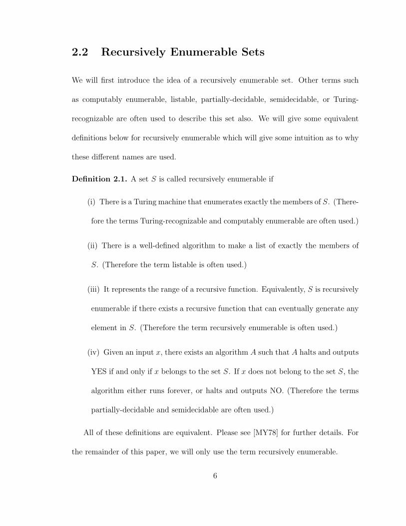
2.2 Recursively Enumerable Sets

We will first introduce the idea of a recursively enumerable set. Other terms such

as computably enumerable, listable, partially-decidable, semidecidable, or Turing-

recognizable are often used to describe this set also. We will give some equivalent

definitions below for recursively enumerable which will give some intuition as to why

these different names are used.

Definition 2.1. A set S is called recursively enumerable if

(i) There is a Turing machine that enumerates exactly the members of S. (There-

fore the terms Turing-recognizable and computably enumerable are often used.)

(ii) There is a well-defined algorithm to make a list of exactly the members of

S. (Therefore the term listable is often used.)

(iii) It represents the range of a recursive function. Equivalently, S is recursively

enumerable if there exists a recursive function that can eventually generate any

element in S. (Therefore the term recursively enumerable is often used.)

(iv) Given an input x, there exists an algorithm A such that A halts and outputs

YES if and only if x belongs to the set S. If x does not belong to the set S, the

algorithm either runs forever, or halts and outputs NO. (Therefore the terms

partially-decidable and semidecidable are often used.)

All of these definitions are equivalent. Please see [MY78] for further details. For

the remainder of this paper, we will only use the term recursively enumerable.

6

We can now state the set of all prime numbers is recursively enumerable. It is

easy to see this by Definition 2.1 (iv). Given a number n, we can test if it is prime by

attempting to divide by every number less than n. Similarly, the exponential function

(ax) and the factorial function also define sets which are recursively enumerable since

we can test membership of any number by a given algorithm

In the next section, we will state that all of these sets are in fact Diophantine

representable.

2.3 Recursively Enumerable Sets are Diophantine

Representable

As an even simpler example than the last two, we can state that the set of even

numbers forms a recursively enumerable set, since we can test if a number is even

with a simple algorithm. More so, since the set of even numbers is precisely {x such

that there exists y ∈ Z and y = 2x}, the Diophantine system representing even

numbers is given by the single equation y = 2x (where x, y ∈ Z).

The main positive aspect of the negative solution to Hilbert’s Tenth Problem

is that every Diophantine set is a recursively enumerable set and every recursively

enumerable set is Diophantine representable. For more information on this, please

see [Mat70] and [DMR76].

Therefore, we know that the set of primes must also be Diophantine representable.

7

The question remains how to represent them. This was shown by Martin Davis, Yuri

Matijasevic, and Julia Robinson.

The derivation of the system is out of the scope of this paper. If the reader is

interested in seeing it, please refer to [JSWW76]. It would also be helpful to look

through [Dav73] as a bare minimum. In the next section, we will give the Diophantine

system.

2.4 Diophantine Representation of the Set of Primes

The system has been expressed in slightly different forms in different papers. There

have been minor changes in representation only. Here is the system given by [JSWW76]

with a slight modification so that all variables belong to the set of non-negative in-

tegers. In this system there is a solution for all variables if and only if k + 2 is

prime.

q = wz + h + j, (2.1)

z = (gk + 2g + k + 1)(h + j) + h, (2.2)

16(k + 1)3(k + 2)(n + 1)2 + 1 = f 2, (2.3)

e = p + q + z + 2n, (2.4)

e3(e + 2)(a + 1)2 + 1 = o2, (2.5)

x2 = (a2 − 1)y2 + 1, (2.6)

8

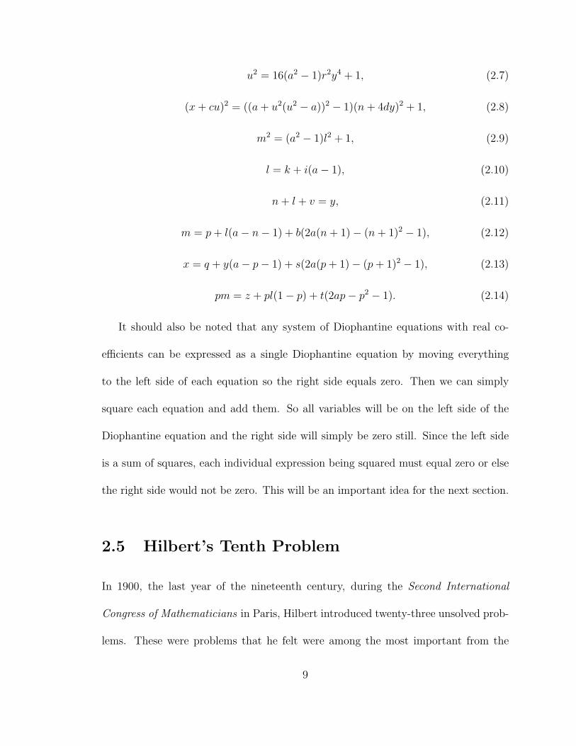
u2 = 16(a2 − 1)r2y4 + 1, (2.7)

(x + cu)2 = ((a + u2(u2 − a))2 − 1)(n + 4dy)2 + 1, (2.8)

m2 = (a2 − 1)l2 + 1, (2.9)

l = k + i(a− 1), (2.10)

n + l + v = y, (2.11)

m = p + l(a− n− 1) + b(2a(n + 1)− (n + 1)2 − 1), (2.12)

x = q + y(a− p− 1) + s(2a(p + 1)− (p + 1)2 − 1), (2.13)

pm = z + pl(1− p) + t(2ap− p2 − 1). (2.14)

It should also be noted that any system of Diophantine equations with real co-

efficients can be expressed as a single Diophantine equation by moving everything

to the left side of each equation so the right side equals zero. Then we can simply

square each equation and add them. So all variables will be on the left side of the

Diophantine equation and the right side will simply be zero still. Since the left side

is a sum of squares, each individual expression being squared must equal zero or else

the right side would not be zero. This will be an important idea for the next section.

2.5 Hilbert’s Tenth Problem

In 1900, the last year of the nineteenth century, during the Second International

Congress of Mathematicians in Paris, Hilbert introduced twenty-three unsolved prob-

lems. These were problems that he felt were among the most important from the

9

nineteenth century and which would continue into the upcoming twentieth century.

Since then, these have been labelled “Hilbert’s Twenty-Three Problems.”

What follow is a translation into English of the tenth problem exactly as it was

stated:

10. Determination of the solvability of a Diophantine equation. Given a

diophantine equation with any number of unknown quantities and with

rational integral numerical coefficients: To devise a process according to

which it can be determined by a finite number of operations whether the

equation is solvable in rational integers.

Equivalently, this can be stated as: Is it possible to find an algorithm which will

tell us whether or not a polynomial Diophantine equation with integer coefficients

has integer solutions?

A negative proof to Hilbert’s Tenth Problem was given by Matijasevic in [Mat70].

He proved that every recursively enumerable set is Diophantine representable. More

so, there are undecidable recursively enumerable sets such as x such that Mx halts on input x

where Mx denotes the Turing Machine whose code is x. This is the set of codes that

halts on itself as input. The problem of determining whether a code will halt on

itself is called the Halting Problem. (A definition for Turing Machine can be found

in [MY78]).

Now we would like to discuss how to solve the particular Diophantine system

representing the set of primes. However, we will need to provide the next two chapters

10

before we can do this.

11

Chapter 3

Continued Fractions

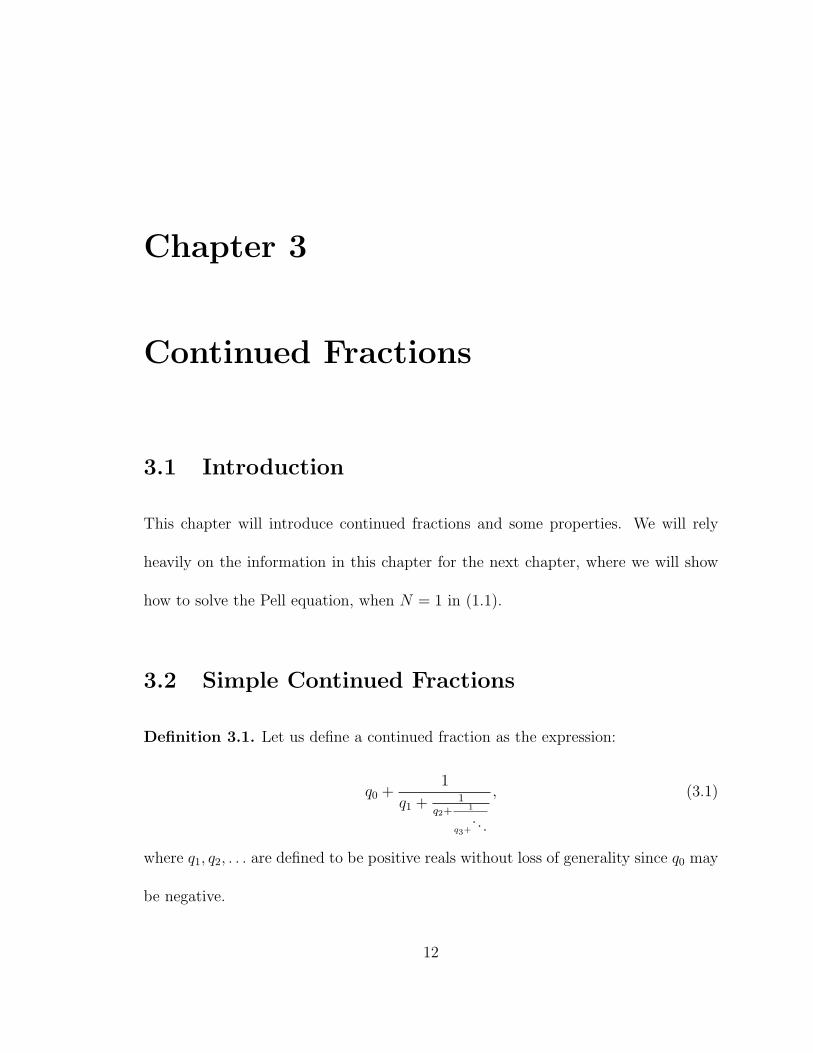
3.1 Introduction

This chapter will introduce continued fractions and some properties. We will rely

heavily on the information in this chapter for the next chapter, where we will show

how to solve the Pell equation, when N = 1 in (1.1).

3.2 Simple Continued Fractions

Definition 3.1. Let us define a continued fraction as the expression:

q0 +1

q1 + 1q2+ 1

q3+...

, (3.1)

where q1, q2, . . . are defined to be positive reals without loss of generality since q0 may

be negative.

12

Now, let’s define a simple continued fraction.

Definition 3.2. If q0, q1, q2, . . . ∈ Z, then the continued fraction is called a simple

continued fraction.

We should introduce some quick notation for the continued fraction also.

Definition 3.3. Use the notation < q0, q1, q2, q3, . . . > to express the continued frac-

tion in Definition 3.1.

The following proposition is very easy to see from Definition 3.1, but will prove

to be very useful in proofs later.

Proposition 3.1. < q0, q1, . . . , qn, qn+1 >=< q0, q1, . . . , qn−1, qn + 1qn+1

> .

We will now define convergents of the continued fraction, which we will use in a

later lemma.

Definition 3.4. Define rn =< q0, q1, . . . , qn >, for every n > 0. These are called the

convergents of the continued fraction.

We will now define two sequences of great importance to the study of continued

fractions, and then state and prove a lemma relating the convergents from Definition

3.4 to these sequences.

Definition 3.5. Define h−2 = 0, h−1 = 1, k−2 = 1, k−1 = 0. For every i ≥ 0, define

hi = hi−1qi + hi−2, (3.2)

ki = ki−1qi + ki−2. (3.3)

13

Lemma 3.1. For every n ≥ 0, rn = hn

kn.

Proof. We will prove this by induction. The base case n = 0 can be checked quickly:

r0 =h0

k0

=h−1q0 + h−2

k−1q0 + k−2

=q0

1= q0. (3.4)

For the induction hypothesis, assume rn = hn

kn. Define

h′ = (qn +1

qn+1

)hn−1 + hn−2, (3.5)

k′ = (qn +1

qn+1

)kn−1 + kn−2. (3.6)

By Proposition 3.1 and the induction hypothesis, h′

k′=< q0, q1, . . . , qk, qn+1 >. Now

let’s look at hn+1 and kn+1

hn+1 = hnqn+1 + hn−1 = (hn−1qn + hn−2)qn+1 + hn−1, (3.7)

kn+1 = knqn+1 + kn−1 = (kn−1qn + kn−2)qn+1 + kn−1. (3.8)

However, it is easy to see now that

h′ =hn+1

qn+1

, k′ =kn+1

qn+1

. (3.9)

So,

rn+1 =hn+1

kn+1

=h′

k′=< q0, q1, . . . , qk, qn+1 > . (3.10)

The value of the simple continued fraction is given by limn→∞rn. We will simply

mention that this limit will always exist. A proof of this can be found in [NZ72]

14

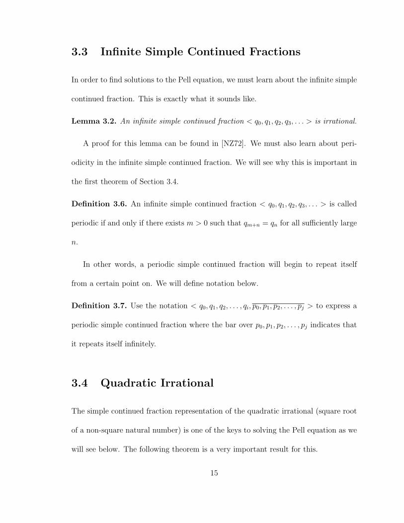
3.3 Infinite Simple Continued Fractions

In order to find solutions to the Pell equation, we must learn about the infinite simple

continued fraction. This is exactly what it sounds like.

Lemma 3.2. An infinite simple continued fraction < q0, q1, q2, q3, . . . > is irrational.

A proof for this lemma can be found in [NZ72]. We must also learn about peri-

odicity in the infinite simple continued fraction. We will see why this is important in

the first theorem of Section 3.4.

Definition 3.6. An infinite simple continued fraction < q0, q1, q2, q3, . . . > is called

periodic if and only if there exists m > 0 such that qm+n = qn for all sufficiently large

n.

In other words, a periodic simple continued fraction will begin to repeat itself

from a certain point on. We will define notation below.

Definition 3.7. Use the notation < q0, q1, q2, . . . , qi, p0, p1, p2, . . . , pj > to express a

periodic simple continued fraction where the bar over p0, p1, p2, . . . , pj indicates that

it repeats itself infinitely.

3.4 Quadratic Irrational

The simple continued fraction representation of the quadratic irrational (square root

of a non-square natural number) is one of the keys to solving the Pell equation as we

will see below. The following theorem is a very important result for this.

15

Theorem 3.1. If an infinite simple continued fraction is periodic, it is a quadratic

irrational.

Proof. Case 1: Simple continued fraction is purely periodic.

β =< p0, p1, p2, . . . , pj > . (3.11)

Then we can say that,

β =< p0, p1, p2, . . . , pj, β > . (3.12)

From Lemma 3.1, we know that

β =hjβ + hj−1

kjβ + kj−1

(3.13)

By rearranging, we know that β is a root of a quadratic equation. Since the simple

continued fraction representation of β is infinite, by Lemma 3.2, we know that β must

be a quadratic irrational.

Case2: Simple continued fraction is not purely periodic.

α =< q0, q1, . . . , qi, p0, p1, p2, . . . , pj > . (3.14)

Let us define β (similar to (3.11)) as

β =< p0, p1, p2, . . . , pj > . (3.15)

Now we can write (similar to (3.12))

α =< q0, q1, . . . , qi, β > . (3.16)

16

We know that (similar to (3.13))

α =hiβ + hi−1

kiβ + ki−1

(3.17)

We also know that β is of the form

a +√

b

c(3.18)

for some a, b, c. Again, by Lemma 3.2, we know that α cannot be rational. Then by

(3.17) and (3.18), we know that α must be a quadratic irrational also.

The converse of the above theorem also holds. A proof of this can be found in

[NZ72].

Let’s go through a quick example to make sure we understand this clearly before

moving on to the next chapter.

Example 3.1. Let us find x, where x =< a, b, a, b, . . . >=< a, b > . Alternatively, we

can write x as

x = a +1

b + 1x

. (3.19)

This is simply a quadratic, which we can solve. The solutions to this quadratic are

ab±√

a2b2 + 4ab

2b. (3.20)

17

Chapter 4

Solving the Pell Equation

4.1 Introduction

From here on, when we say Pell equation, we will always be talking about the special

case of the Pell equation (1.1), when N = 1. In this chapter, we will walk through one

way of solving the Pell equation. The basic idea will be to use the simple continued

fraction representation of√

d (from (1.1)) to find the minimal solution of the Pell

equation.

This chapter will provide many of the ideas necessary to solve the Diophantine

system representing the set of primes in the next chapter.

18

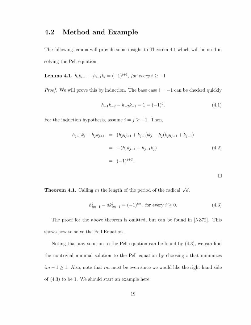
4.2 Method and Example

The following lemma will provide some insight to Theorem 4.1 which will be used in

solving the Pell equation.

Lemma 4.1. hiki−1 − hi−1ki = (−1)i+1, for every i ≥ −1

Proof. We will prove this by induction. The base case i = −1 can be checked quickly

h−1k−2 − h−2k−1 = 1 = (−1)0. (4.1)

For the induction hypothesis, assume i = j ≥ −1. Then,

hj+1kj − hjkj+1 = (hjqj+1 + kj−1)kj − hj(kjqj+1 + kj−1)

= −(hjkj−1 − hj−1kj) (4.2)

= (−1)j+2.

Theorem 4.1. Calling m the length of the period of the radical√

d,

h2im−1 − dk2

im−1 = (−1)im, for every i ≥ 0. (4.3)

The proof for the above theorem is omitted, but can be found in [NZ72]. This

shows how to solve the Pell Equation.

Noting that any solution to the Pell equation can be found by (4.3), we can find

the nontrivial minimal solution to the Pell equation by choosing i that minimizes

im− 1 ≥ 1. Also, note that im must be even since we would like the right hand side

of (4.3) to be 1. We should start an example here.

19

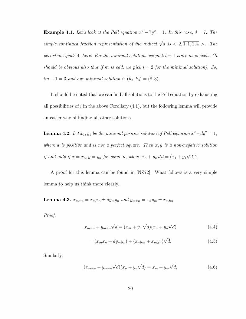
Example 4.1. Let’s look at the Pell equation x2 − 7y2 = 1. In this case, d = 7. The

simple continued fraction representation of the radical√

d is < 2, 1, 1, 1, 4 >. The

period m equals 4, here. For the minimal solution, we pick i = 1 since m is even. (It

should be obvious also that if m is odd, we pick i = 2 for the minimal solution). So,

im− 1 = 3 and our minimal solution is (h3, k3) = (8, 3).

It should be noted that we can find all solutions to the Pell equation by exhausting

all possibilities of i in the above Corollary (4.1), but the following lemma will provide

an easier way of finding all other solutions.

Lemma 4.2. Let x1, y1 be the minimal positive solution of Pell equation x2−dy2 = 1,

where d is positive and is not a perfect square. Then x, y is a non-negative solution

if and only if x = xn, y = yn for some n, where xn + yn

√d = (x1 + y1

√d)n.

A proof for this lemma can be found in [NZ72]. What follows is a very simple

lemma to help us think more clearly.

Lemma 4.3. xm±n = xmxn ± dymyn and ym±n = xnym ± xmyn.

Proof.

xm+n + ym+n

√d = (xm + ym

√d)(xn + yn

√d) (4.4)

= (xmxn + dymyn) + (xnym + xmyn)√

d. (4.5)

Similarly,

(xm−n + ym−n

√d)(xn + yn

√d) = xm + ym

√d, (4.6)

20

implies

xm−n + ym−n

√d = (xm + ym

√d)(xn − yn

√d) (4.7)

= (xmxn − dymyn) + (xnym − xmyn)√

d (4.8)

Note that we used the fact that x2n − dy2

n = 1 above since xn and yn are solutions to

our Pell equation.

4.3 Special Pell Equation

In this section, we will look at the special case of the Pell equation (1.1) where

d = a2 − 1, a > 1, N = 1. (4.9)

Notice that in this case, we have another obvious solution, in addition to (1.4):

x1 = a, y1 = 1. (4.10)

Below, we will give a simple Corollary from Lemma 4.2.

Corollary 4.1. Let us define xn = xn(a) and yn = yn(a) such that all solutions to

this special Pell equation must be of this form:

xn + yn

√d = (a +

√d)n, for every a > 1 and for every n ≥ 0. (4.11)

This corollary is very easy to see by a simple substitution from (4.10).

The following Corollary is a special case of Lemma 4.3, when n = 1 for the special

Pell equation.

21

Corollary 4.2. xm±1 = axm ± dym and ym±1 = aym ± xm.

Proof. Letting n = 1 in Lemma (4.3), we have

xm±1 = xmx1 ± dymy1, (4.12)

ym±1 = x1ym ± xmy1. (4.13)

Remembering that x1 = a and y1 = 1, let’s make these substitutions into (4.12) so

we get xm±1 = axm ± dym and ym±1 = aym ± xm.

22

Chapter 5

Solving the Diophantine System

Representing the Set of Primes

5.1 Introduction

The proof of the system given in Section 2.4 is provided with an excellent explanation

in [JSWW76]. There are also other papers with the proof provided. So, I will not

repeat it here. Instead, I will provide some insight into how to solve the system, given

the proof.

As I go through the method for solving the system, I will drop some ideas from

the proof to help explain what we are doing. It will quickly become obvious that this

Diophantine representations for the set of primes relies heavily on the Pell equation,

exponential function, and factorial function. However, I strongly recommend reading

23

the proof for a complete understanding.

Also, I should again mention here that we are solving the representation provided

earlier in Section 2.4. The original representation by Matiyasevich in 1970 differed

somewhat ([Mat70]). There were also a number of other Diophantine representations

of the primes with less variables. However, with less variables, the polynomial degree

of the Diophantine system increased greatly. A description of these along with some

other Diophantine representations are provided in [Rib91].

5.2 Method

For the system to be satisfied, we assume a selected value of k ≥ 0 and k + 2 is a

prime number. Let’s provide Wilson’s Theorem as our first lemma here.

Lemma 5.1 (Wilson’s Theorem). For every, k ≥ 0, k + 2 is a prime number if

and only if (k + 2)|((k + 1)! + 1).

A proof of this lemma can be found in [NZ72]. This lemma tells us that if k + 2

is prime, we can pick a number g such that

(k + 1)! = gk + 2g + k + 1. (5.1)

Note that this means (k + 1)! + 1 = (g + 1)(k + 2). Let us now give the following

lemma which defines the factorial function by a Diophantine system.

Lemma 5.2. In order for fk = k +1! for fk, k ≥ 0, it is necessary and sufficient that

24

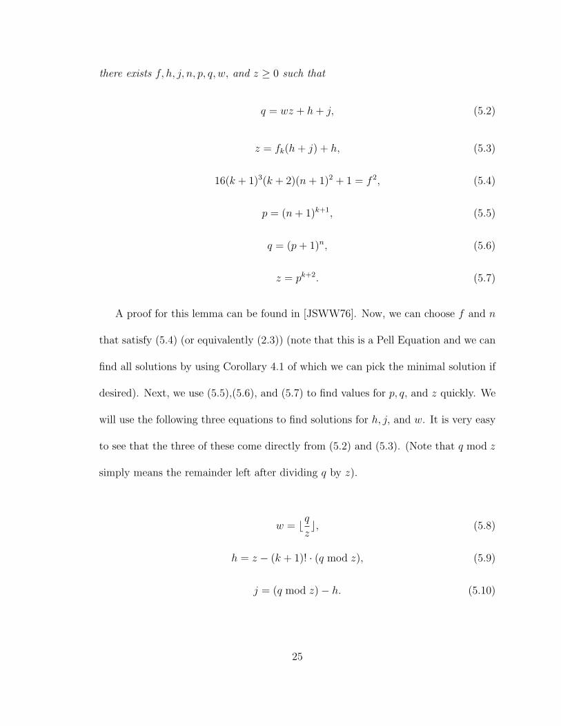
there exists f, h, j, n, p, q, w, and z ≥ 0 such that

q = wz + h + j, (5.2)

z = fk(h + j) + h, (5.3)

16(k + 1)3(k + 2)(n + 1)2 + 1 = f 2, (5.4)

p = (n + 1)k+1, (5.5)

q = (p + 1)n, (5.6)

z = pk+2. (5.7)

A proof for this lemma can be found in [JSWW76]. Now, we can choose f and n

that satisfy (5.4) (or equivalently (2.3)) (note that this is a Pell Equation and we can

find all solutions by using Corollary 4.1 of which we can pick the minimal solution if

desired). Next, we use (5.5),(5.6), and (5.7) to find values for p, q, and z quickly. We

will use the following three equations to find solutions for h, j, and w. It is very easy

to see that the three of these come directly from (5.2) and (5.3). (Note that q mod z

simply means the remainder left after dividing q by z).

w = bqzc, (5.8)

h = z − (k + 1)! · (q mod z), (5.9)

j = (q mod z)− h. (5.10)

25

Then, we can choose e that satisfies (2.4) easily. We can choose a ≥ 2 and o that

satisfy (2.5) by noticing that this is also a Pell equation. Let

y = yn(a) (5.11)

(from Definition 4.1). Next, let us give the following lemma which defines a particular

solution to the Pell equation.

Lemma 5.3. In order for y = yn(a) for a ≥ 2 and n ≥ 1, it is necessary and

sufficient that there exists c, d, r, u, and x such that

x2 = (a2 − 1)y2 + 1, (5.12)

u2 = 16(a2 − 1)r2y4 + 1, (5.13)

(x + cu)2 = ((a + u2(u2 − a))2 − 1)(n + 4dy)2 + 1, (5.14)

n ≤ y. (5.15)

A proof for this lemma can also be found in [JSWW76]. The first three equations

above are exactly the same as (2.6), (2.7), and (2.8). We can find x satisfying the Pell

equation (2.6). Then, we can find u and r again by solving the Pell equation (2.7).

Finally, we can find c and d satisfying the Pell equation (2.8). We know that a

solution exists since a, x, y, and u are now fixed. So the remaining equation in (2.8)

is simply a Pell equation on variables c and d.

m = xk+1(a) (5.16)

26

and

l = yk+1(a). (5.17)

This will satisfy (2.9). Choose i, v, b, s, and t that satisfy (2.10), (2.11), (2.12),(2.13),

and (2.14), respectively. If any of these do not turn out to be integers, we will have

to make another choice for the solution of the Pell equation we chose earlier.

Again, we did not completely show necessity and sufficiency above. Instead we

can find this is in [JSWW76]. In the next section, we will go through the example of

the prime 2, where we try to solve for all variables.

27

Chapter 6

Example: Prime Two

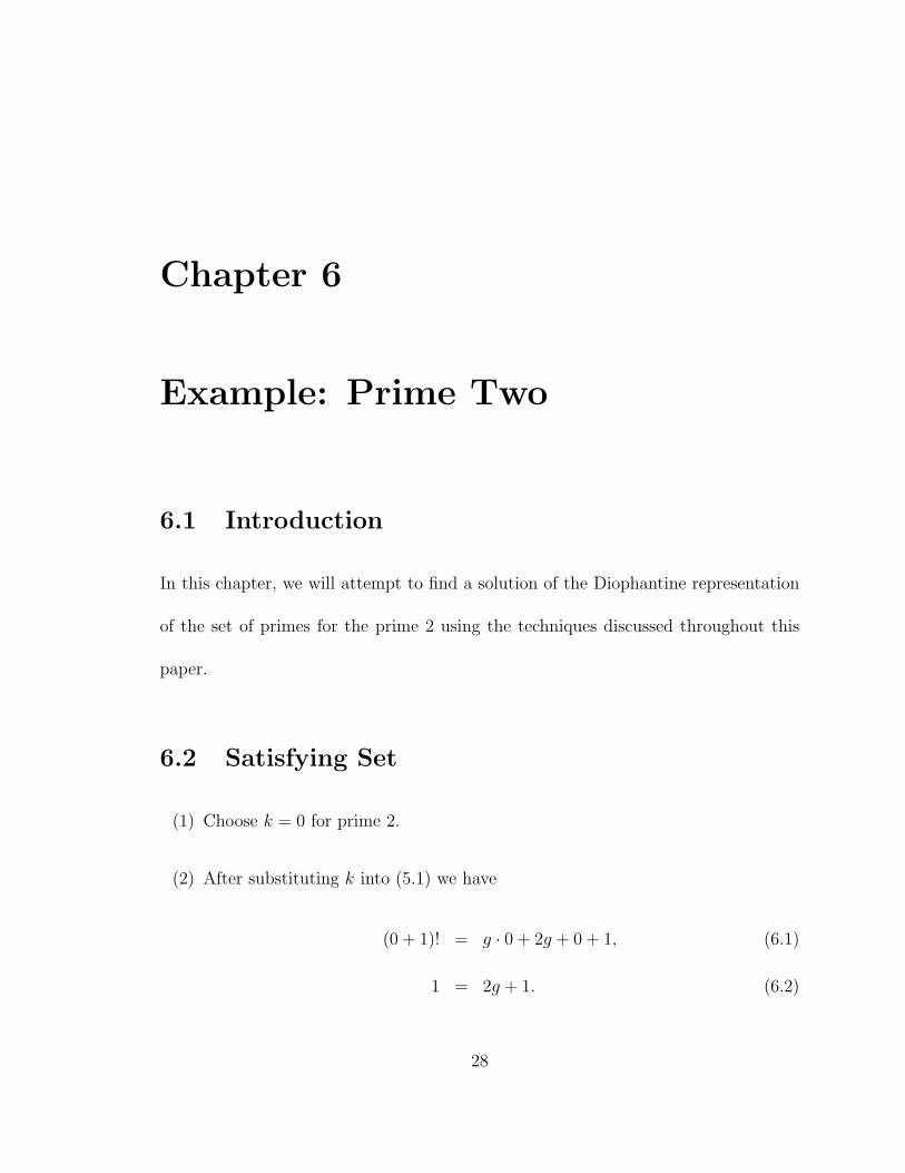
6.1 Introduction

In this chapter, we will attempt to find a solution of the Diophantine representation

of the set of primes for the prime 2 using the techniques discussed throughout this

paper.

6.2 Satisfying Set

(1) Choose k = 0 for prime 2.

(2) After substituting k into (5.1) we have

(0 + 1)! = g · 0 + 2g + 0 + 1, (6.1)

1 = 2g + 1. (6.2)

28

Choose g = 0 to satisfy this equation.

(3) After substituting k into (2.3) we have

16(0 + 1)3(0 + 2)(n + 1)2 + 1 = f 2, (6.3)

f 2 − 32(n + 1)2 = 1 (6.4)

In order to find f and n, we must find a solution to the Pell equation (6.4). The

continued fraction representation of√

32 =< 5, 1, 1, 1, 10 >. So, if we choose

the minimal solution, we have (f, n + 1) = (h3, k3). This gives (f, n) = (17, 2).

(4) After substituting k and n into (5.5) we have

p = (2 + 1)0+1 (6.5)

Choose p = 3 to satisfy this equation.

(5) After substituting n and p into (5.6) we have

q = (3 + 1)2 (6.6)

Choose q = 16 to satisfy this equation.

(6) After substituting k and p into (5.7) we have

z = 30+2 (6.7)

Choose z = 9 to satisfy this equation.

29

(7) After substituting q and z into (5.8) we have

w = b16

7c (6.8)

Choose w = 1 to satisfy this equation.

(8) After substituting k, q, and z into (5.9) we have

h = 9− (0 + 1)! · (16 mod 9), (6.9)

h = 9− (7). (6.10)

Choose h = 2 to satisfy this equation.

(9) After substituting h, q, and z into (5.10) we have

j = (16 mod 9)− 2, (6.11)

j = (7)− 2. (6.12)

Choose j = 5 to satisfy this equation.

(10) After substituting n, p, q, and z into (2.4) we have

e = 3 + 16 + 9 + 2(2) (6.13)

Choose e = 32 to satisfy this equation.

(11) After substituting e into (2.5) we have

323(32 + 2)(a + 1)2 + 1 = o2, (6.14)

o2 − 21617(a + 1)2 = 1 (6.15)

30

In order to find a, o, we must find a solution to the Pell equation (6.15). The

minimal solution given our selection of variables thus far gives

a = 7901690358098896161685556879749949186326380713409290912 and

o = 8340353015645794683299462704812268882126086134656108363777.

To see why, please see the next section.

(12) After substituting n into (5.11) we have

y = y2(a) (6.16)

We know that the minimal solution (x1, y1) = (a, 1) from (4.10). So y2 = 2a by

Corollary 4.2 here.

(13) We can now either solve (5.12) directly or we can note that since y = y2(a),

x must be x2(a) in order to be a solution pair to the Pell equation. x2(a) =

ax1 + (a2 − 1) = 2a2 − 1. We used (4.10) and Corollary 4.2 here.

(14) After substituting k into (5.16) and (5.17) we have

m = x0+1(a) = a (6.17)

l = y0+1(a) = 1 (6.18)

We used (4.10) here.

(15) After substituting k, l into (2.10) we have

1 = 1 + i(a− 1) (6.19)

31

Since we know a− 1 6= 0, we choose i = 0 to satisfy this equation.

(16) After substituting l, n, y into (2.11) we have

2 + 1 + v = 2a (6.20)

We choose v = 2a− 3 to satisfy this equation.

(17) After substituting l,m, n, p into (2.12) we have

a = 3 + 1(a− 2− 1) + b(2a(2 + 1)− (2 + 1)2 − 1), (6.21)

a = 3 + a− 3 + b(6a− 9− 1), (6.22)

0 = b(6a− 10). (6.23)

(6.24)

Since we know 6a− 10 6= 0, choose b = 0 to satisfy this equation.

(18) After substituting p, q, x, y into (2.13) we have

2a2 − 1 = 16 + 2a(a− 3− 1) + s(2a(3 + 1)− (3 + 1)2 − 1), (6.25)

2a2 − 1 = 16 + 2a2 − 8a + s(8a− 16− 1), (6.26)

8a− 17 = s(8a− 17). (6.27)

(6.28)

Since we know 8a− 17 6= 0, choose s = 1 to satisfy this equation.

32

(19) After substituting l,m, p, z into (2.14) we have

3 · a = 9 + 3 · 1(a− 3) + t(2a · 3− 32 − 1), (6.29)

3a = 9 + 3a− 9 + t(6a− 10), (6.30)

0 = t(6a− 10). (6.31)

(6.32)

Since we know 6a− 10 6= 0, choose t = 0 to satisfy this equation.

We provided values for 22 of the 26 variables above (for the prime 2). There

will be a note about the other four in section 6.4. It should also be noted that we

attempted to pick the smallest values for each variable whenever possible given past

choices. This does not ensure that each variable above has the smallest possible value

for the prime two. However, for many of the large variables it is unlikely that there

will be smaller possible values.

6.3 Proof of Minimal Solution for a and o

We would like to find the minimal solution of the Pell equation o2−21617(a+1)2 = 1

or equivalently, x2 − 21617y2 = 1, where x = o and y = a + 1.

Let’s look at two ways of doing this. The first way will be the same method we

have been using thus far, while the second way will investigate a slightly different

way.

33

Method 1

The continued fraction representation of√

216 · 17 =< 1055, 1, 1, 16, 8, 5, 2, 1, 1, 2, 1, 2,

32, 1, 1, 1, 1, 1, 1, 2, 3, 2, 7, 1, 4, 3, 1, 1, 2, 1, 131, 4, 1, 1, 4, 3, 7, 1, 14, 1, 1, 8, 32, 1, 6, 1, 1, 5, 2,

1, 7, 1, 1, 3, 1, 1, 1, 2, 527, 2, 1, 1, 1, 3, 1, 1, 7, 1, 2, 5, 1, 1, 6, 1, 32, 8, 1, 1, 14, 1, 7, 3, 4, 1, 1, 4,

131, 1, 2, 1, 1, 3, 4, 1, 7, 2, 3, 2, 1, 1, 1, 1, 1, 1, 32, 2, 1, 2, 1, 1, 2, 5, 8, 16, 1, 1, 2110 >. This

has period 116. So, we want (x, y) = (h115, k115). This gives (x, y) = (834035301564579

4683299462704812268882126086134656108363777, 790169035809889616168555687974

9949186326380713409290913). This is the smallest possibility for x, y since we picked

the minimal solution here.

However, in this method, we did not discuss how we generated the continuous

fraction and how we knew the period is 116. Let us look at another approach below,

which may be much easier to do in some cases.

Method 2

Let’s look at the similar Pell equation where d is square free: X2 − 17Y 2 = 1. The

continued fraction representation of√

17 =< 4, 8 >. So, we want (X, Y ) = (h1, k1).

This gives (X, Y ) = (33, 8). We now want to find the minimal solution of this same

Pell equation restricting the second term to be divisible by√

216 = 28. In this way,

we can find a solution to the original Pell equation.

First we note that in this case, Xn is always odd. The following lemma will prove

this.

34

Lemma 6.1. Xn satisfying X2 − 17Y 2 = 1 is odd for every n ≥ 1.

Proof. This will be a proof by induction. The base case holds since X1 = 33. Assume

for our induction hypothesis that Xn is odd for n = m. We will now want to show

that it is also odd for Xm+1. Xm+1 = 33Xm + 17 · 8Ym (use Lemma 4.3). From our

induction hypothesis, the first term is odd. It is obvious that the second term is even.

Therefore, Xm+1 is odd.

Next, we notice that Y2n = 2XnYn. It is easy to see that we need to choose Y25 to

make sure that it is divisible by 28 (this can be proven by Lemma 4.3). Now we notice

that when we go back to the original Pell equation, we can choose o = X25 and a+1 =

Y25

28 . By Lemma 4.2, this gives a = 790169035809889616168555687974994918632638071

3409290912 and o = 8340353015645794683299462704812268882126086134656108363777

like before.

6.4 The Other Four Variables

We can certainly show how to find the variables c, d, r, u, which are missing above.

However, these variables grow to be so large that it would be physically impossible

to compute them.

Let’s apply the process used in Method 2 above to (2.7). Let’s look at the similar

Pell equation where d is square free: U2− (a2−1)R2 = 1. In this case we will want to

find the minimal solution of this Pell equation with the restriction that R is divisible

35

by√

16y4 = 4y2. This would give us a solution to our original Pell equation. The

prime factorization of 4y2 is

21669123573485147475984154163149818989665876594781436961512.

This means that we would need at least y357348514747598415416314981898966587659478143696151

(by Lemma 6.3) which is already more than 1052 decimal places (we will show why

later).

We can see that u must be even bigger than r by the Pell equation. The numbers

c and d are part of another Pell equation in (2.8) that rely on a value of u (and are

probably even larger than u).

Lemma 6.2.

(xn, yn) = 1.

Proof. Assume k|xn, k|yn, then k|(x2n−dy2

n). This implies k|1 since x2n−dy2

n = 1.

Lemma 6.3. Let p be a prime and let n be the smallest positive integer such that p

divides yn. Assume in addition that p2 does not divide yn. Then ynp is the smallest

value that is divisible by p2.

Proof. Assume p2 divides ym for some m < np. Then m = kn + r, where 0 ≤ r < n

36

and k > 0. Then, we have

xr + yr

√d = (x1 + y1

√d)r (6.33)

= (x1 + y1

√d)m−kn (6.34)

= (x1 + y1

√d)m · (x1 + y1

√d)−kn (6.35)

= (x1 + y1

√d)m · (x1 − y1

√d)kn (6.36)

= (xm + ym

√d) · (xn − yn

√d)k (6.37)

Since both ym and yn are divisible by p we conclude that yr is also divisible by p.

But n was chosen as the smallest positive integer, such that p divides yn. Therefore,

r must be 0 and n divides m so that m = kn for some k > 1.

So we have

xkn + ykn

√d = (xn + yn

√d)k (6.38)

=k∑

i=0

(k

i

)xk−i

n (yn

√d)i. (6.39)

This implies

ym = ykn =∑

i odd,1≤i≤k

(k

i

)xk−i

n yind

i−12 (6.40)

If i ≥ 2, then p2 obviously divides yin since p divides yn. But we also need the

term for i = 1 to be divisible by p2. This term is

kxknyn. (6.41)

Since xn and yn are relatively prime (by Lemma 6.2), we also know that xn and p

are relatively prime since p divides yn. Further, since p2 does not divide yn, we must

37

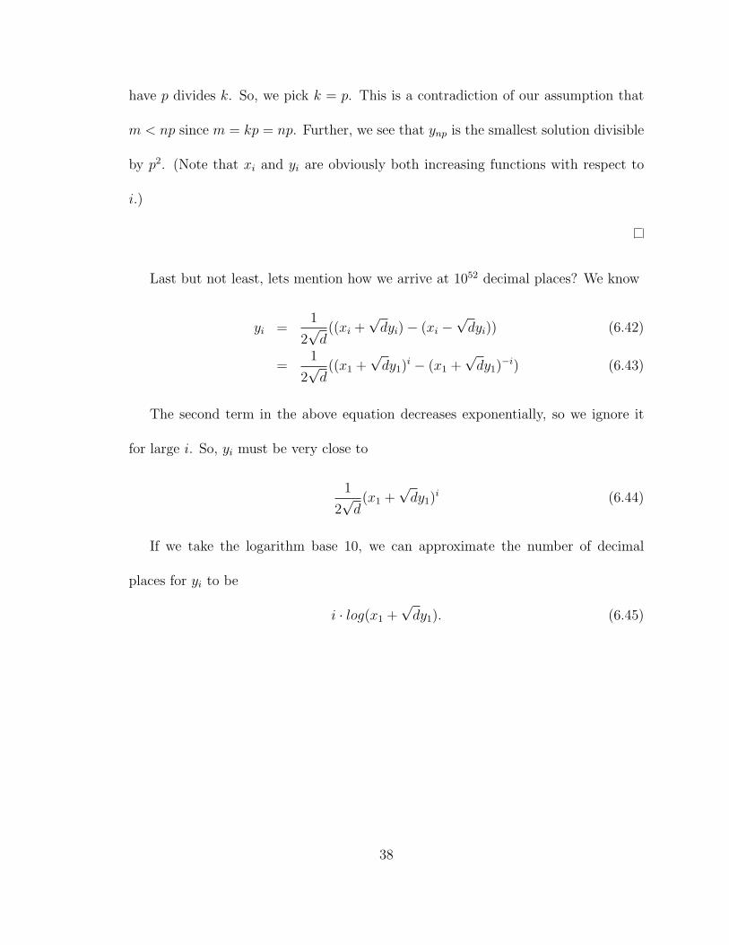
have p divides k. So, we pick k = p. This is a contradiction of our assumption that

m < np since m = kp = np. Further, we see that ynp is the smallest solution divisible

by p2. (Note that xi and yi are obviously both increasing functions with respect to

i.)

Last but not least, lets mention how we arrive at 1052 decimal places? We know

yi =1

2√

d((xi +

√dyi)− (xi −

√dyi)) (6.42)

=1

2√

d((x1 +

√dy1)

i − (x1 +√

dy1)−i) (6.43)

The second term in the above equation decreases exponentially, so we ignore it

for large i. So, yi must be very close to

1

2√

d(x1 +

√dy1)

i (6.44)

If we take the logarithm base 10, we can approximate the number of decimal

places for yi to be

i · log(x1 +√

dy1). (6.45)

38

Appendix A

Acknowledgements

Special thanks to (in alphabetical order):

Dr. Martin Davis for some e-mail correspondence.

Dr. Dennis DeTurck for acting on my academic committee and discussing the

details of the paper with me.

Dr. Herbert Enderton for some discussion meetings.

Dr. Jean Gallier for acting as my academic advisor for this research. He also

introduced me to [DMR76], which began my interest in this whole area.

Dr. Yuri Matiyasevich for some e-mail correspondence and introducing me to Dr.

Vsemirnov.

Dr. Max Mintz for acting as my academic advisor in the Computer Science De-

partment and providing me with academic guidance.

Dr. Maxim Vsemirnov for kindly providing much assistance and guidance via only

39

e-mail correspondence and proofreading the entire thesis.

And last but not least, the Mathematics Faculty and Staff at the University of

Pennsylvania for providing me with the facilities and guidance to complete this re-

search. The Mathematics Department not only contains a unique faculty and student

body but also a wonderful staff.

On another note, I should also thank the researchers of Hilbert’s Tenth Problem.

There are so many people who made significant contributions here.

40

Bibliography

[Buc46] R. C. Buck. Prime-representing functions. American Mathematical

Monthly, 53(5):265, May 1946.

[Dav73] Martin Davis. Hilbert’s Tenth Problem is unsolvable. The American

Mathematical Monthly, 80(3):233–269, March 1973. Reprinted with cor-

rections in the Dover edition of Davis [1958].

[Dav82] Martin Davis. Computability and Unsolvability. Dover, 1982.

[DMR76] Martin Davis, Yuri Matijasevic, and Julia Robinson. Hilbert’s Tenth

Problem. Diophantine equations: positive aspects of a negative solution.

In Mathematical Developments Arising from Hilbert Problems, volume 28

of Proceedings of Symposia in Pure Mathematics, pages 323–378, Provi-

dence, Rhode Island, 1976. American Mathematical Society.

[Dud69] Underwood Dudley. History of a formula for primes. American Mathe-

matical Monthly, 76(1):23–28, January 1969.

41

[HW79] G. H. Hardy and E. M. Wright. An Introduction to the Theory of Numbers.

Oxford Clarendon Press, fifth edition, 1979.

[Jon82] James P. Jones. Universal Diophantine equation. Journal of Symbolic

Logic, 47(3):549–571, September 1982.

[JSWW76] James P. Jones, Daihachiro Sato, Hideo Wada, and Douglas Wiens. Dio-

phantine representation of the set of prime numbers. The American Math-

ematical Monthly, 83(6):449–464, June–July 1976.

[Len02] Lenstra. Solving the pell equation. NOTICES: Notices of the American

Mathematical Society, 49, 2002.

[Mat70] Ju. V. Matijasevic. Enumerable sets are Diophantine. Soviet Mathemat-

ics. Doklady, 11(2):354–358, 1970.

[Mat93] Yu. V. Matiyasevich. Hilbert’s Tenth Problem. MIT Press, Cambridge,

Massachusetts, 1993.

[Mat00] Matiyasevich. Hilbert’s tenth problem: What was done and what is to be

done. In Denef, Lipshitz, Pheidas, and Van Geel, editors, Hilbert’s Tenth

Problem: Relations with Arithmetic and Algebraic Geometry, AMS, 2000.

2000.

[MY78] Michael Machtey and Paul Young. An Introduction to the General Theory

of Algorithms. Thomond Books, 1978.

42

[NZ72] I. Niven and H. S. Zuckerman. An Introduction to the Theory of Numbers.

Wiley, 1972.

[Rei43] Irving Reiner. Functions not formulas for primes. American Mathematical

Monthly, 50(10):619–621, December 1943.

[Rib91] Paulo Ribenboim. The Little Book of Big Primes. Springer-Verlag, New

York, 1991.

[Sma98] Nigel P. Smart. The Algorithmic Resolution of Diophantine Equations.

Cambridge University Press, 1998.

[Sør97] Morten Heine Sørensen. Hilbert’s tenth problem. In Computability and

Complexity from a Programming Perspective (D-295), Foundations of

Computing, pages 167–185. MIT Press, Boston, London, 1 edition, 1997.

[ST86] T. N. Shorey and R. Tidjeman. Exponential Diophantine Equations. Cam-

bridge University Press, 1986.

[Wri51] E. M. Wright. A prime-representing function. American Mathematical

Monthly, 58(9):616–618, November 1951.

43