Finding a (Food) Way: A GIS Modeling Approach to Quantifying Local Food Transportation Systems

Anna G. Bovbjerg

A thesis

submitted in partial fulfillment of the

requirements for the degree of

Master of Science in Civil Engineering

University of Washington

2017

Committee:

Anne Goodchild

Edward McCormack

Program Authorized to Offer Degree:

Department of Civil and Environmental Engineering

i

© Copyright 2017

Anna G. Bovbjerg

ii

University of Washington

Abstract

Finding a (Food) Way: A GIS Modeling Approach to Quantifying Local Food Transportation Systems

Anna G. Bovbjerg

Chair of the Supervisory Committee:

Anne Goodchild, PhD

Department of Civil and Environmental Engineering

In recent years the focus on and prioritization of the notion of local food, food access and

sustainability has been increasing throughout the U.S., especially in urban areas. The rising

demand and growing preference for local produce in turn leads to changes in how we transport

food. The supply chains found in urban areas are already complicated and costly, and as demand

changes this poses a challenge if the local food movement is to be accommodated in our cities.

A new initiative seeks to mitigate these challenges through the introduction of a mobile application

that allows users to order local produce online. Logistics modeling was conducted as a case study

to support this effort. The goal of the research was to be able to inform and support decision-

making on the logistics to support agricultural development and equal food access. The research

found that there is opportunity for improvement to how local food is accessed, and that these

mobile applications have the possibility to address food accessibility, economic vitality and

sustainability, with a lower negative impact on the transportation environment.

iii

ACKNOWLEDGEMENTS

The act of researching, writing and completing a Master’s thesis is a lonely endeavor. That doesn’t

mean, that one must be alone, and thankfully I wasn’t. I would like to thank my faculty advisor

and chair of my reading committee Dr. Anne Goodchild, for her guidance and support, both

professionally and personally; and for the opportunities and development she has given me. I know

I am not only speaking for myself when I say what a great inspiration she is. I’d furthermore like

to thank Dr. Edward McCormack for his advice both on this work, and on much else; I’m looking

forward to our continued collaboration. I’m incredibly grateful for the lovely group up people who

are working for the Supply Chain Transportation and Logistics Center at the University of

Washington – you ladies (and gents) are kickass, and I want all the best in the world for you.

This research was conducted with support from the Valle Scandinavian Scholarship and Exchange

Program – I will always be thankful for this opportunity.

;

iv

TABLE OF CONTENTS Table of Contents ......................................................................................................................... iv

List of Figures ................................................................................................................................ v

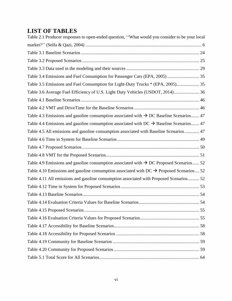
List of Tables ................................................................................................................................ vi

Acronyms ..................................................................................................................................... vii

Glossary of Terms ....................................................................................................................... vii

1. Introduction ........................................................................................................................... 1

1.1 Statement of Problem ....................................................................................................... 2

2. Literature Review ................................................................................................................. 5

2.1 Local Food and Values ..................................................................................................... 6

2.2 Decreasing VMT in Food Transportation ...................................................................... 10

2.3 Food Access ................................................................................................................... 13

3. Methodology ........................................................................................................................ 15

3.1 Modeling Scenarios ........................................................................................................ 15

3.2 ArcGIS and Network Analyst ........................................................................................ 27

3.3 Evaluation Criteria ......................................................................................................... 33

4. Analysis and Results ........................................................................................................... 39

4.1 Analysis of Baseline Scenarios ...................................................................................... 46

4.2 Analysis of Proposed Scenarios ..................................................................................... 50

4.3 Results and Comparison of Scenarios ............................................................................ 54

5. Conclusion ........................................................................................................................... 61

5.1 Questions for Further Research ...................................................................................... 66

6. References ............................................................................................................................ 69

v

LIST OF FIGURES Figure 3.1 Vashon-Maury Island, Washington ............................................................................. 17

Figure 3.2 Household income divisions from Vashon survey results .......................................... 20

Figure 3.3 Total Logistics Cost Tradeoff (McKinnon, 2003) ....................................................... 26

Figure 3.4 Dijkstra’s Algorithm can be used to find the shortest path from one point to the other

(Ryan, 2004). ................................................................................................................................ 28

Figure 4.1 Routing Map of Customers to Distribution Center ..................................................... 40

Figure 4.2 Routing Map of Farmers to Distribution Center ......................................................... 41

Figure 4.3 Routing Map of Customers to Individual Farms ......................................................... 42

Figure 4.4 Routing Map from Distribution Center to all Customers and Farmers ....................... 43

Figure 4.5 Routing Map of Roundtrip from Farmers to Distribution Center ............................... 44

Figure 4.6 Routing Map of Roundtrip from Customers to Distribution Center ........................... 45

Figure 4.7 Relative comparison of emissions and gasoline consumption between the four scenarios

....................................................................................................................................................... 48

Figure 4.8 Comparison of Time in System for Baseline Scenarios .............................................. 50

Figure 4.9 Relative Comparison of Pollutants and Gasoline Consumption ................................. 52

Figure 4.10 Comparison of Time in System for Proposed Scenarios ........................................... 54

Figure 4.11 Comparison of Values for Baseline Scenarios .......................................................... 55

Figure 4.12 Comparison of Values for Proposed Scenarios ......................................................... 56

Figure 4.13 Miles/Person Roundtrip for All Scenarios ................................................................ 57

Figure 4.14 Comparison of All Scenarios by Evaluation Criteria ................................................ 57

Figure 5.1 Total Score for All Scenarios ...................................................................................... 66

vi

LIST OF TABLES Table 2.1 Producer responses to open-ended question, ‘‘What would you consider to be your local

market?’’ (Selfa & Qazi, 2004) ...................................................................................................... 6

Table 3.1 Baseline Scenarios ........................................................................................................ 24

Table 3.2 Proposed Scenarios ....................................................................................................... 25

Table 3.3 Data used in the modeling and their sources ................................................................ 29

Table 3.4 Emissions and Fuel Consumption for Passenger Cars (EPA, 2005) ............................ 35

Table 3.5 Emissions and Fuel Consumption for Light-Duty Trucks * (EPA, 2005) .................... 35

Table 3.6 Average Fuel Efficiency of U.S. Light Duty Vehicles (USDOT, 2014) ...................... 36

Table 4.1 Baseline Scenarios ........................................................................................................ 46

Table 4.2 VMT and DriveTime for the Baseline Scenarios ......................................................... 46

Table 4.3 Emissions and gasoline consumption associated with DC Baseline Scenarios ....... 47

Table 4.4 Emissions and gasoline consumption associated with DC Baseline Scenarios ....... 47

Table 4.5 All emissions and gasoline consumption associated with Baseline Scenarios ............. 47

Table 4.6 Time in System for Baseline Scenarios ........................................................................ 49

Table 4.7 Proposed Scenarios ....................................................................................................... 50

Table 4.8 VMT for the Proposed Scenarios .................................................................................. 51

Table 4.9 Emissions and gasoline consumption associated with DC Proposed Scenarios ...... 52

Table 4.10 Emissions and gasoline consumption associated with DC Proposed Scenarios .... 52

Table 4.11 All emissions and gasoline consumption associated with Proposed Scenarios .......... 52

Table 4.12 Time in System for Proposed Scenarios ..................................................................... 53

Table 4.13 Baseline Scenarios ...................................................................................................... 54

Table 4.14 Evaluation Criteria Values for Baseline Scenarios ..................................................... 54

Table 4.15 Proposed Scenarios ..................................................................................................... 55

Table 4.16 Evaluation Criteria Values for Proposed Scenarios .................................................... 55

Table 4.17 Accessibility for Baseline Scenarios........................................................................... 58

Table 4.18 Accessibility for Proposed Scenarios ......................................................................... 58

Table 4.19 Community for Baseline Scenarios ............................................................................ 59

Table 4.20 Community for Proposed Scenarios ........................................................................... 59

Table 5.1 Total Score for All Scenarios........................................................................................ 64

vii

ACRONYMS

FDA Food and Drug Administration GIS Geographic Information Systems

CSA Community Supported Agriculture WSDOT Washington State Department of Transportation

VMT Vehicle Miles Traveled TSP Traveling Salesman Problem

VRP Vehicle Routing Problem O-D Origin-Destination

VRPTW Vehicle Routing Problem with Time Windows

GLOSSARY OF TERMS ArcGIS

A propriety software package that allows the user to

work with GIS. The main components of the program

are ArcMap and ArcCatalog, though the software can

be expanded using extensions.

Community Supported Agriculture

Agricultural cooperation programs which allows

farmers to sell directly to its end customers, and

customers to obtain local food, through a seasonal or

weekly membership program.

Farm Stands

Road side stands, which allow the customer to buy

produce directly from the farm, without the typical

store front set-up.

Farmers Markets

Usually weekly markets where farmers set up booths

with their produce and products in the same location,

and allows for the customers to access many different

farms at one location.

Food System

The system in which we move our food. Includes

production, storage, packaging, transportation, retail

outlets and distribution.

Local Food

Food produced in a certain vicinity from the end

consumer. There is not a consensus on the distance that

limits the notion of local, but it is usually considered

local within state and within larger region (e.g. the

Puget Sound region in WA or the region of Western

Washington)

Network Analyst

A proprietary software extension of ArcGIS. It allows

for the users to activate the road network, so that it can

be used for modeling and analysis purposes.

Vehicle Miles Traveled

A measure of distance commonly used to compare

transportation systems

viii

1 of 71

1. INTRODUCTION

In recent years the focus on and prioritization of the notion of local food, food access and

sustainability has been increasing throughout the United States. The rising demand to know where

our food comes from and a growing preference for local produce in turn leads to changes in how

we transport food. This is especially apparent in urban areas, which are often more separated from

their food environment than rural areas. The supply chains found in urban areas are already

exceedingly complicated and costly, and as demand changes this poses a challenge if the local

food movement is to be accommodated in our cities. Farmers Markets and local food delivery

systems are often criticized for carrying significantly higher impacts on emissions and the overall

transportation system, which ends up decreasing or diminishing the potential positive impact that

buying locally produced food could have had.

A new initiative backed by the King County Conservation District in King County, Washington,

seeks to mitigate these different challenges through the introduction of a mobile application that

allows users to order local produce online from Vashon Island farmers, and logistics modeling was

conducted as a case study to support this effort. The research presents a variety of logistics designs,

which were modeled and compared to each other and to the status quo. The goal of the research

was to be able to inform decision-making on the logistics of sourcing and distributing local food,

to support agricultural development and equal food access.

2 of 71

1.1 Statement of Problem

The research conducted and presented in this paper is based on the following research question:

How can local food transportation systems be

structured to allow for local food access without

incurring negative transportation impacts?

This Statement of Problem is examined through the following sub questions:

1) What is research currently discussing regarding the state of local food distribution

systems in the U.S.?

2) What are the reasonable assumptions and appropriate evaluation criteria for

modeling and assessing food distribution systems using GIS?

3) Comparing different food transportation system structures, which systems offer the

best solution for improving access to local food?

Question 1 is examined and answered through the Literature Review found in Chapter 2, where

local food systems, their structures, values, customers and issues are examined. This section

furthermore examines VMT in Food Transportation and other efforts to model food transportation

system.

Chapter 0 presents the methodology of the project and answers Question 2 by describing the

background for the project, the baseline and proposed scenarios, and necessary assumptions. It

furthermore describes the chosen tools for the modeling effort, along with the selected evaluation

criteria. Finally, it includes a discussion of the limitations of the decisions made in this section.

3 of 71

The final Question 3 is examined in Chapter 0. In this the methodology from the previous section

is applied and the results are presented and discussed. It both compares current conditions, the

baseline scenarios, to each other, but also compares the potential, proposed scenarios, to both each

other and the baseline. It discusses implications of selecting the different structures and the

tradeoffs associated with the different decisions.

Chapter 5 presents the conclusion of the project along with questions for further research, and

answers the overall Statement of Problem.

4 of 71

5 of 71

2. LITERATURE REVIEW

When examining food distribution, and especially the supply chains that support the food industry

and food access in the U.S., one quickly realizes that these systems are uniquely different from

other supply chain networks, and that this has significant impact on how we construct this network.

Food supply chains are much more complex and more difficult to manage, as there are different

concerns that needs to be addressed. Food supply chains frequently operate under strict time

constraints to avoid spoilage of products, and as it is known, imposing constraints on a supply

chain network always increases cost. The threat of spoilage also means that food usually must be

transported in refrigerated container units – reefers – which are costly to run, both to the

carrier/shipper, but also in terms of environmental impact. Another concern that is present in food

supply chains is the fear of contamination. In the US the most recent standard, the FDA’s Food

Safety Modernization Act (FSMA) rule on Sanitary Transportation of Human and Animal Food,

was most recently updated in 2016, and sets requirements for vehicle and transportation equipment

(e.g. cleanliness of the container), transportation operations (e.g. adequate temperature controls),

training in sanitary operations and record keeping (FDA, 2016). Once again this increases the cost

of transporting food, compared to non-food items that are covered by less strict regulation

regarding quality and tracking. Another thing that increases cost in the supply chain, is the fact

that food often has a high weight-to-value ratio; Potatoes e.g. are a relatively heavy item, but

doesn’t carry much value. It therefore takes a lot of potatoes to cover the cost of transporting them,

which usually means highly consolidated transportation systems amongst others. There are several

other concerns regarding food transportation: Food is fragile and the quality quickly decreases

under the wrong conditions; it requires unique packaging, and is seldom square and efficient to

pack and load; it is dependent on nature, meaning that when a food item is not locally or naturally

6 of 71

available, it is necessary to source it from distance areas, use long-term storage or use energy-

intensive alternatives, such as greenhouses (Wakeland, et al., 2012). For these reasons amongst

others, it is necessary to study food systems separately from other types of supply chain systems.

The following section will further describe existing areas of research related to food distribution

systems.

2.1 Local Food and Values

Local food involves purchasing food stuff from producers within a certain vicinity or range from

the end consumer. There is currently not a set standard or limit on the geographic boundary for

when the products are considered local. Research done in Washington State asked producers in

three counties, one of which is King County where the City of Seattle is located, and found that

most producers considered the state, Northwest region and their county and adjacent counties their

local food market. The table below shows the responses sorted by county:

Table 2.1 Producer responses to open-ended question, ‘‘What would you consider to be your local market?’’ (Selfa & Qazi, 2004)

Grant County. Chelan County. King County. Proximity 8.2 4.3 3.7 Within county or adjacent county 19.6 39.0 66.0 Washington State or northwest region 26.3 21.0 9.2 US/world 8.2 11.6 0.0 Social relations (producer–consumer links) 6.5 2.8 7.4 Contract/ intermediary 24.5 11.6 12.9 None/ don’t know 6.5 8.0 0.0 n 61 69 54

Looking at the table above it seems that the boundaries for when something is considered local is

dependent on the spatial context it participates in (Selfa & Qazi, 2004).

Local food interest has been increasing in recent years. There are several reasons for why

consumers seek out local food. These reasons encompass both consideration of intrinsic and

7 of 71

extrinsic factors, which are enabled and moderated through characteristics of the consumer. These

include both demographic and social characteristics (Khan, 1981; Shepherd, 1989; Grunert, 1997).

Local food is not a consideration to the same degree in developing countries as it is in developed

countries, suggesting that credence factors, such as healthiness, environmental benefits and animal

welfare are just as moderating for the behavior as the nature of the product (Gracia & Albisu, 2001;

Mannion, 2000).

Though the notion of local food belongs in the developed world, it is wide-spread throughout and

does not necessarily relate to a certain social group or level of income or affluence. Contrary to

organic food’s perception as being higher-cost and indicative of a certain demographic group, local

food is not. In fact, researchers reviewing 73 papers found that local food isn’t not perceived as

being costlier to the consumer, or belonging to a specific demographic or group of consumers

(Feldmann & Hamm, 2014). However, they find that that reason for not buying local food more

often is related to purchase barriers: inconvenience in shopping for local food and a lack of

availability (Feldmann & Hamm, 2014).

There are both benefits to local food and challenges for the producers as well. (Mount, 2011)

argues that local food is a “value-added, multi-generational alternative to the poor profitability and

dwindling prospects of conventional commodity production” (Mount, 2011, p. 116). For small

scale farms, scaling the operation and reaching the customers does have its own challenges. The

primary barriers are logistical, structural and regulatory in nature (Mount, 2011).

2.1.1 Farmers Markets, CSAs and Farm Stands

Farmers markets have a long history, but saw a decline in mid-1900s as refrigerators, supermarkets

and convenience food became more prevalent in the U.S. During the 60s and 70s the number of

8 of 71

farmers markets started to increase, and from 1960 to 1994 it increased from around 100 to almost

1,800 markets nationwide, and from 1994 to 2011 to more than 7,100 markets (USDA, 2012).

Today Farmers Markets, CSAs and Farm Stands are popular ways to access produce that are

originating locally, and especially in more urban areas, where access and connection to agriculture

is limited, these initiatives are continuing to gain traction, and seem to be more successful, than in

rural areas (Gasteyer, et al., 2008).

Farmers Markets are traditionally held on weekends, though nightly Farmers Markets are

becoming more common. Producers from local areas will pack the harvest of the week and drive

it to a central location, where a booth is setup for customers to visit. The markets are usually open

4-7 hours in the middle of the day, and will in addition to produce also offer flowers, prepared

products and non-foods. In literature, the use of Farmers Markets is additional to a household’s

general consumption, and that the activity of visiting a Farmers Market is more of a community

building activity, than merely the necessity to acquire food for the household. In a review, the

author writes that: “(…) for the large majority of them, ‘‘local’’ food is not primarily about

distance from the source of the food. Instead, it is much more about the establishment of

connections between food consumption and food production, and firmly rooting these in a specific

place. ‘‘Local,’’ then, unlike food miles, is not really a spatial concept at all. Food, for many, has

become an important part of direct experience and sensory input in shaping their experience of

place” (Schnell, 2013, p. 11). Another paper further supports this claim, and says that: “(…)

farmers market impacts on communities were making a place for social activity and promoting a

sense of community, in addition to providing fresh food for consumers and positive economic

impacts for local businesses “ (Oberholtzer & Grow, 2003). For farmers participating in farmers

markets, around 31% of them only sell their produce through that outlet, and the remaining 69%

9 of 71

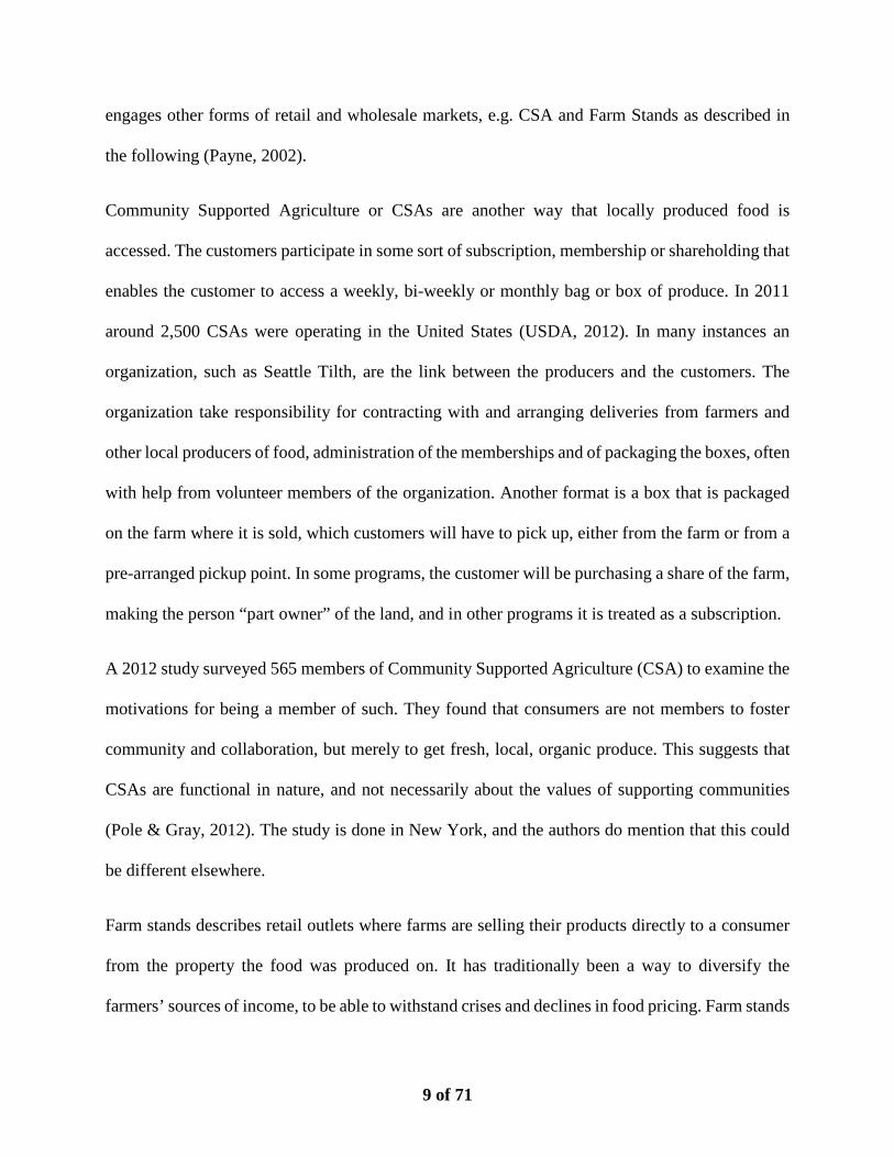
engages other forms of retail and wholesale markets, e.g. CSA and Farm Stands as described in

the following (Payne, 2002).

Community Supported Agriculture or CSAs are another way that locally produced food is

accessed. The customers participate in some sort of subscription, membership or shareholding that

enables the customer to access a weekly, bi-weekly or monthly bag or box of produce. In 2011

around 2,500 CSAs were operating in the United States (USDA, 2012). In many instances an

organization, such as Seattle Tilth, are the link between the producers and the customers. The

organization take responsibility for contracting with and arranging deliveries from farmers and

other local producers of food, administration of the memberships and of packaging the boxes, often

with help from volunteer members of the organization. Another format is a box that is packaged

on the farm where it is sold, which customers will have to pick up, either from the farm or from a

pre-arranged pickup point. In some programs, the customer will be purchasing a share of the farm,

making the person “part owner” of the land, and in other programs it is treated as a subscription.

A 2012 study surveyed 565 members of Community Supported Agriculture (CSA) to examine the

motivations for being a member of such. They found that consumers are not members to foster

community and collaboration, but merely to get fresh, local, organic produce. This suggests that

CSAs are functional in nature, and not necessarily about the values of supporting communities

(Pole & Gray, 2012). The study is done in New York, and the authors do mention that this could

be different elsewhere.

Farm stands describes retail outlets where farms are selling their products directly to a consumer

from the property the food was produced on. It has traditionally been a way to diversify the

farmers’ sources of income, to be able to withstand crises and declines in food pricing. Farm stands

10 of 71

allow the farmers to retain a much higher percentage of the cost of the food, as there are no

middlemen and they do not have to offer the produce at wholesale price (ACS, 2017).

2.2 Decreasing VMT in Food Transportation

When products are moved from their location of production to the distributor and end consumer,

negative impacts are incurred, such as pollution, wear and a decrease in quality. A measure that

has popularly been used is food miles, which is an idea based on person-travel, but by a unit of

produce. There are however some issues with using food miles to describe food distribution

systems; there are not any agreements on the units used and what to include and exclude from

calculations, and used in studies it ends up as a qualitative measure, as opposed to the quantitative

measure it was intended to be. (Schnell, 2013) criticizes the unsupported use food miles as the

average amount of miles a product travels in the U.S. and tracks the origin of these numbers. A

1,500-mile figure stems from a (Pirog, Pelt, Enshayan, & Cook, 2001) who found that unprocessed

U.S produce sold at the Chicago Terminal Produce Market on average travelled 1,518 miles. A

1,300-mile figure stems from a 1969 report written by the U.S. army, and doesn’t use any food

transportation data at all. (Hora & Tick, 2001) found that fruits sold in Jessup, Maryland travels

2,146 miles and vegetables 1,685.5 miles on average per pound, but had the same limitations as

the Pirog study. (Weber & Matthews, 2008) found that the average ton of food travels 1,019 miles

in delivery only, but 4,200 miles during its entire life cycle. None of these studies are without

serious limitations, according to the author. (Schnell, 2013) The fact is, that we do not know how

far our food travels on average.

What is more applicable in isolated situations, such as case studies is comparing different

distribution systems. (Coley, et al., 2008) completed a comparison of farm shop and mass

distribution approaches, in relation to local food, food miles and carbon emissions. They found

11 of 71

that if a consumer drives more than 6.7 kilometers roundtrip to buy organic produce, the

environmental gain of doing so will likely be outweighed and it may be more environmentally

friendly to buy from a super market. This is however only including energy in the forms of

electricity and fuel. (Mundler & Rumpus, 2012) made a comparison of different modes of

distribution within local food systems in terms of energy efficiency in Lyon, France. They found

that local food sales can have a better energy score, but doesn’t necessarily, which the authors

conclude leave room for improvement. They do point out, as (Coley, Howard, & Winter, 2008)

does, that fuel is not enough of an attribute to compare by, as it doesn’t fully encompass all the

economic and social factors of local vs. non-local produce.

One method attempted have been made to make grocery shopping more efficient and convenient,

is by offering online grocery shopping. In recent years companies like Blue Apron and Plated have

started to offer meals sent as pre-packaged ingredients, that the consumer then cooks themselves.

Grocery stores are also entering into the market, with delivery systems such as Instacart and

Amazon Prime, and Amazon itself are running their own online grocer Amazon Fresh now.

Conducted in 1990, a survey found that customers in the Netherlands who shopped for groceries

online made less trips overall. Their average frequency was 0.4 trips/weekday, compared to the

national standard of 1.0 trips/weekday. These customers were more likely to supply their online

shopping with local shopping, as opposed to visiting supermarkets. They also found that online

grocery shopping was less frequent, though that could be for other reasons than necessity to buy.

Of the surveyed customers who used online grocery shopping, 70% believed that it saved them

time. Only 20% of the surveyed customers answered the question of what they spent their time on

instead, but the original author comments that no new activities are added, but the time is instead

12 of 71

added to existing activities, such as sleeping or watching television, and that “Most people did not

mention any new activity that required travel”.

In a self-reporting study from the UK, 74% of the 160 responding users of an online grocery

shopping platform, said that they drove less because of their online shopping. A statistical study

found that consumers who buy groceries online spend less time on shopping travel, take less

shopping trips, and overall travel shorter distances. Consumers reported that they believed that the

primary time saving from buying groceries online, stemmed from the decrease in transportation.

(Morganosky & Cude, 2000). An author found in 2001, that purchasing groceries online resulted

in a reduction of four trips/month. It was noted that this is double of what is seen in non-grocery

shopping reductions. The author concludes that the impact of grocery shopping is complex, but

that the less frequent shopping associated with online groceries, may lead to reduction in overall

VMT. (Cairns, 2004). Only one author found a different result: A paper comparing online shopping

travel behavior, noted that travel behavior was influenced in four different ways: substitution,

modification, complementarity and neutrality. The study found that buying groceries online

increased shopping trips and trip chaining, as most of the behavior is complimentary. (Ferrell,

2004).

(Lanzendorf, 2004) concludes that consumers who buy groceries online use the” net time savings

for longer periods of social, recreation or leisure activities, at home or outdoors”, but that the

impact of this on VMT and mobility is unknown by the research community. As the previous

author, this article also finds that the use of online grocery shopping in itself probably does not

lead to a travel reduction, as the freight transportation is increased, but that behavior associated

with it may help to mitigate this increase. (Lanzendorf, 2004)

13 of 71

Several other studies have considered grocery shopping frequency in-store vs. online, but are all

conducted before 2002, and at a time where delivery charges for many platforms were very high

(Kärnä, 2001; Burke, 1998). No recent literature was found regarding frequency. (Mokhtarian,

2004)

2.3 Food Access

Looking at the literature presented there is an interest in enhancing the access to local food

throughout communities in the US, though there are still barriers to do so. These barriers are not

necessarily price or consumption, but to a higher degree challenges of access. The research at hand

examines access to food in a constrained geographical area. Access can be defined in many ways,

including access by mode split and time access modeling. For the purposes of this research, the

access to food is regarded as vehicular, and that access is improved when the point of access is

more central and/or closer to the end consumer.

14 of 71

15 of 71

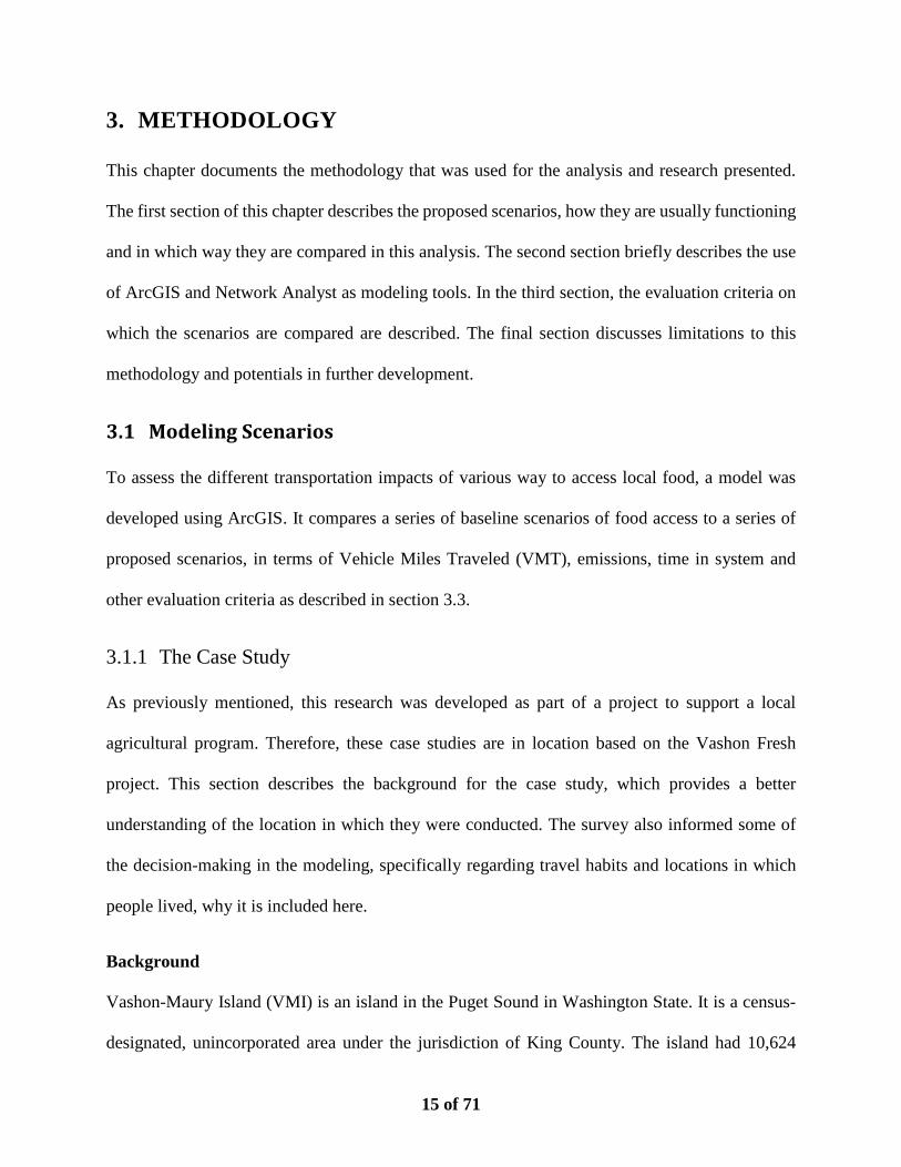
3. METHODOLOGY

This chapter documents the methodology that was used for the analysis and research presented.

The first section of this chapter describes the proposed scenarios, how they are usually functioning

and in which way they are compared in this analysis. The second section briefly describes the use

of ArcGIS and Network Analyst as modeling tools. In the third section, the evaluation criteria on

which the scenarios are compared are described. The final section discusses limitations to this

methodology and potentials in further development.

3.1 Modeling Scenarios

To assess the different transportation impacts of various way to access local food, a model was

developed using ArcGIS. It compares a series of baseline scenarios of food access to a series of

proposed scenarios, in terms of Vehicle Miles Traveled (VMT), emissions, time in system and

other evaluation criteria as described in section 3.3.

3.1.1 The Case Study

As previously mentioned, this research was developed as part of a project to support a local

agricultural program. Therefore, these case studies are in location based on the Vashon Fresh

project. This section describes the background for the case study, which provides a better

understanding of the location in which they were conducted. The survey also informed some of

the decision-making in the modeling, specifically regarding travel habits and locations in which

people lived, why it is included here.

Background

Vashon-Maury Island (VMI) is an island in the Puget Sound in Washington State. It is a census-

designated, unincorporated area under the jurisdiction of King County. The island had 10,624

16 of 71

inhabitants at the last census and covers approximately 37 square miles (U.S. Census Bureau,

2010). Today the approximated population is 11,500 people, and the percentage of inhabitants over

the age of 16 years in the civilian work force is 65.4%. VMI does not have any bridge connection,

but does have two ferry docks, that connects the island to the rest of the state. From the south, the

ferry route Tahlequah-Point Defiance had approximately 768,000 riders in 2015 (WSDOT, 2015).

From the north terminal, two ferry routes take riders to either Southworth (175,000 riders

(WSDOT, 2015)) and Fauntleroy (1,950,000 riders (WSDOT, 2015)) in West Seattle, from where

connections can be made to the rest of the City of Seattle. In addition to this, a WSDOT water taxi

running from the North to Downtown Seattle is also available on weekdays. A map of Vashon-

Maury Island can be seen in the figure below.

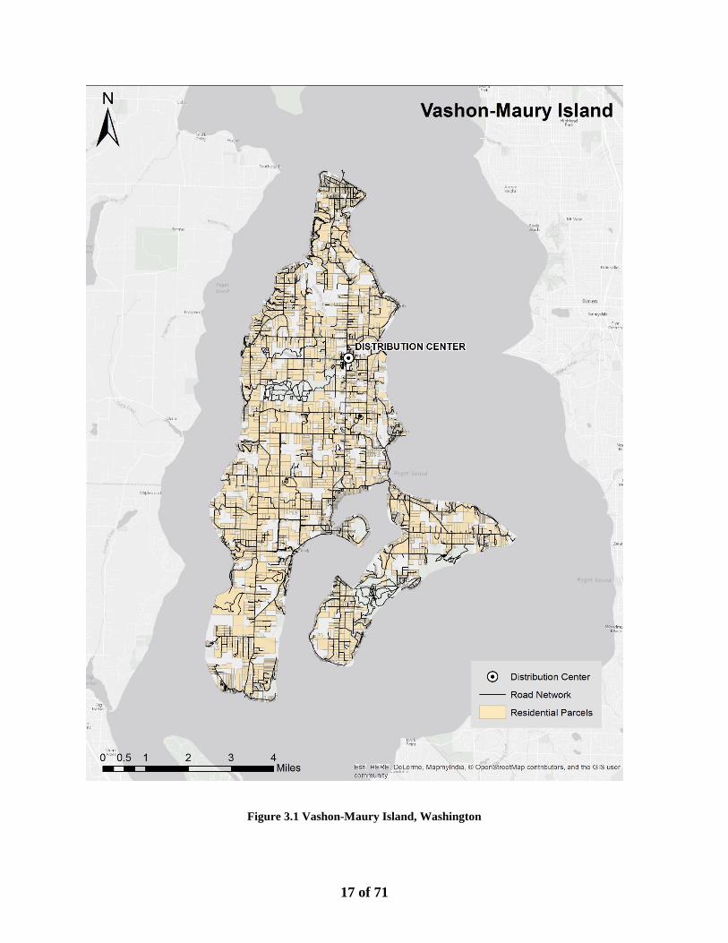
17 of 71

Figure 3.1 Vashon-Maury Island, Washington

18 of 71

Demographics and Surveying Vashon Island

The mean travel time to work for workers above the age of 16 years is 43.9 minutes, which is

significantly higher than the average Washington State (25.9 minutes), King County (27.4

minutes) and City of Seattle (26 minutes) (U.S. Census Bureau, 2010). The median household

income on VMI is $72,568 compared to $73,035 in King County, $67,365 in City of Seattle and

$60,294 in the State of Washington (U.S. Census Bureau, 2010).

The research included conducting a survey of potential customers of the local food service, which

for this study includes everyone who lives on Vashon Island. During the month of March 2017, a

questionnaire was distributed, which asked participants about their current transportation behavior

and their habits relating to their grocery shopping. The full survey can be found in Appendix C,

but includes questions of whether they work on or off Vashon Island, which modes of

transportation they generally use and the respondent’s trip chaining habits.

The survey was distributed using several different channels in hope of reaching as many

participants as possible, as well as an accurate a presentation and distribution of respondents. The

survey was designed as a structured questionnaire, which primarily relied on respondents picking

the most appropriate option. No Likert-scales were included. Only a few questions allow for

respondents to add comments or fill in a blank. To further incentivize participation, respondents

were offered the opportunity to enter their email-address for a chance to win an Amazon-gift card.

The survey was distributed using the following channels:

• Sharing a link to the survey with members of Vashon Island-oriented Facebook Groups

• Sharing the survey with subscribers of VIGA’s newsletter

19 of 71

A total of 201 respondents participated in the survey between March 1st, 2017 and May 15th, 2017.

This number is not representative of the entire population of the island. To reach a 95% confidence

level with an approximated population of 11,500 people a total number of 372 respondents would

have been required, for a confidence interval of ±5. As the total sample is 201 out of the

approximately 11,500 people, the confidence interval for the survey is determined to be ±6.85 at

a 95% confidence level. This variation is larger than what is generally accepted, but for the intents

of using the data for modeling it is acceptable. A larger sample could possibly have been obtained

by sharing the survey on the water taxi or the ferry, though this was unfortunately not possible

under the time constraints. Seeking out survey participants in this way also has the unfortunate

effect of skewing the results, as the answers would then be more representative of the opinions of

commuters. Either way there are benefits and drawbacks, though more data is always better.

Females were strongly overrepresented in the survey with a 77.5%/21.00% split (n=200). This can

be for several reasons, but the most relevant one is probably that female household members are

much more likely to oversee, interested in or have knowledge of their family’s grocery shopping

and food habits. Generally, Vashon Island has a slight overrepresentation of females

(51.3%/48.5%). The age group of the sample was relatively like the one found in the population.

The median age of residents on the island is 51.6 years and it was found that 72.63% of the sample

were between 35 and 64 years of age (n=146). The median was found to be 50-64 and the mean

35-49(n=201). In the 2010 census 32.8 of the population was between 50 and 64 years of age,

close to the 37.31% found in the survey. Families were slightly overrepresented in the survey and

found that 69% of the respondents were married or in a domestic relationship (n=200) where it is

62% in the population.

20 of 71

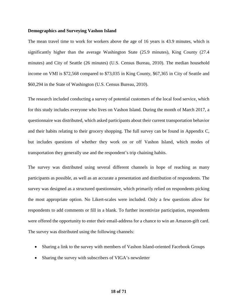
The mean household size of the sample was 2.56 persons and 33% of the respondents had children

under the age of 18 living at home. The mean household size of the population is 2.1 The median

household income on Vashon Island is $71,820, which is slightly lower than the rest of King

County, but significantly higher than Washington State. The survey found a median income

between $80,000 and $99,000 per year. 37% of the respondents reported a median household

income of more than $100,000 per year (n=201). The percentage of people living below the

poverty line was not calculated, as this depends on household size and age and wasn’t found to be

directly relevant. However, 7% of all respondents had a household income of less than $20,000

per year, which is close to the federal poverty level of a family of three, $20,420 per year)

according to the ACS 5-year. The current poverty level of Vashon Island is 5.8%.

Figure 3.2 Household income divisions from Vashon survey results

21 of 71

Summarizing these above points, the survey presents a reasonable picture of the population on

Vashon Island, though with a slightly higher confidence interval than generally accepted. Females,

families, married couples and high-income are overrepresented in the survey, though it is

reasonable representing age, household composition, and poverty level. The full survey, including

the survey zones and the results can be found in Appendix B-D.

The Vashon Island Growers’ Association and Vashon Fresh

The Vashon Island Growers’ Association (VIGA) was founded in the 1980s to support on-island

farming jobs. Today their mission is “To promote farming, access to healthy food, and a

sustainable agricultural economy on Vashon Island through education, advocacy, and a vibrant

Farmers market” (VIGA, 2016). In concert with the mission statement and the success of the

Farmers market, VIGA is now attempting to start a delivery service, like Amazon Fresh, where

local produce can be ordered through an app or website, and conveniently picked up by the many

commuters. To do this, VIGA has been granted $50,000 in funding from the King Conservation

District Regional Food System Grant, which seeks to “[promote} sustainable uses of natural

resources through responsible stewardship (…) link producers with consumers and to serve as a

catalyst for making local food production environmentally and economically sustainable” (KCD,

2016). The pilot was launched in June 2017 and is at the time of writing not completed, but is

expected to run for approximately four months (VIGA, 2016).

3.1.2 Comparing Distribution Systems

For this research, a few different scenarios were modeled. The compared baseline scenarios with

the scenarios that will be proposed to improve access to local food. In selecting the relevant

scenarios for comparison, a few factors had to be taken into consideration. First, to compare the

scenarios directly, they had to adhere to a certain comparability. It is in that manner not relevant

22 of 71

to compare directly to the transportation impacts of e.g. a customer shopping at a standard grocery

store. Since part of the analysis is examining the transportation of the produce from where it is

produced to where it is distributed from, this needs to be known to compare products. With the

complexity with which produce gets to a grocery store from all over the country and world, this

comparison was not possible to do fairly, and that form of buying is therefore not compared

directly. As authors mentioned, for many users these products are supplemental or complimentary

to the basic grocery shopping in a household. For all the baseline and proposed scenario, it is valid

that buying at that location is not a “one-stop-shop”, as a grocery store would be.

Another caveat is the availability of products at a store versus at the proposed scenarios. In a

grocery store, the consumer enters and expect to find everything on their list. For the scenarios,

consumers are more flexible. Because this shopping is supplemental and doesn’t contain some of

the basic household stuff, e.g. diapers and cleaning products, consumers are more willing to adapt

what they’re buying, dependent on what is available at the given day. Because the scenarios share

these characteristics, it further enforces that it is relevant to compare them side-by-side.

3.1.3 Baseline Scenarios

The baseline scenarios describe the transportation impacts of three of the ways in which we access

locally produced agriculture today. The following section will discuss the three different forms of

access and some of the assumptions of the modeling. The (code) following the name of the access

form refers to the modeled scenario. Common for all the baseline scenarios, is that they all require

the individual customer to pick up the produce.

Farmers Markets (B1-FM), often held on weekends, and generally more popular in urban areas,

allow customers to browse a wide selection of local producers at a single location. As previously

23 of 71

discussed, the use of Farmers markets is often seen as a more leisurely way to acquire food, as

opposed to fulfilling the necessity of acquiring food. While it serves well to introduce customers

to new farmers or vendors, Farmers markets is one of the most energy-intensive ways of accessing

food. It requires many people to drive heavy items to a location, setting up a booth, potentially

with cold storage, and for the customers to drive there too to visit the market. It is unconsolidated,

and generally not very efficient. (B1-FM: Baseline 1-Farmer’s Market)

Community Supported Agriculture (CSA) is generally a membership-based setup, which allows

members to receive a bag of locally grown produce, in exchange for the membership fee and often

some sort of volunteering to pack produce occasionally. The two main types are: (B2-CSA1)

organizations such as Seattle Tilth, which acquires produce from Farmers, packs it in their own

facilities and has members pick up the produce from a central location. As this somewhat

consolidates the packing and pickup of the produce, it is expected that the transportation impact of

this setup is lower than (B3-CSA2), which is generally one farm that packages produce and allows

the customers to pick up from their location. These are commonly known as farm shares. As

mentioned in the literature review, driving quickly obliterates the positive environmental impact

of choosing alternative produce. (B2/B3-CSA1/2: Baseline 2/3-Community Supported Agriculture

1/2)

Farm Stands (B4-FS) are usually operated by the farm on which it is located. They are generally

placed on the side of the road, and allows customers to pick up popular items such as strawberries,

potatoes, eggs and flowers, without visiting a store. The quality and tracking requirements for food

from farm stands is significantly more lenient, which is a benefit to the farmers. Payment is often

done through an honor-based system, and it does not have the sense of community-connection that

Farmers markets and CSAs do. One difference between the two, is that whereas customers of B3-

24 of 71

CS2 will drive much longer to acquire produce, Farm Stand customers are generally from the

nearby area and will not incur much travel. (B4-FS: Baseline 4-Farm Stand)

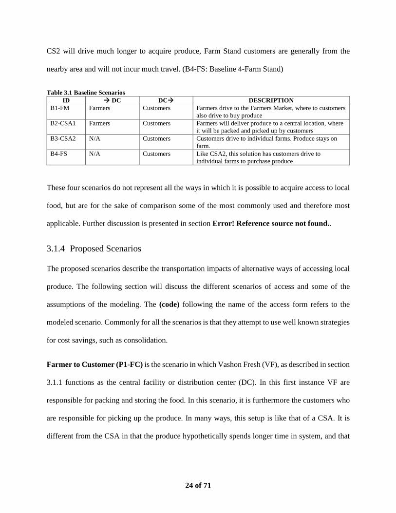
Table 3.1 Baseline Scenarios ID DC DC DESCRIPTION

B1-FM Farmers Customers Farmers drive to the Farmers Market, where to customers also drive to buy produce

B2-CSA1 Farmers Customers Farmers will deliver produce to a central location, where it will be packed and picked up by customers

B3-CSA2 N/A Customers Customers drive to individual farms. Produce stays on farm.

B4-FS N/A Customers Like CSA2, this solution has customers drive to individual farms to purchase produce

These four scenarios do not represent all the ways in which it is possible to acquire access to local

food, but are for the sake of comparison some of the most commonly used and therefore most

applicable. Further discussion is presented in section Error! Reference source not found..

3.1.4 Proposed Scenarios

The proposed scenarios describe the transportation impacts of alternative ways of accessing local

produce. The following section will discuss the different scenarios of access and some of the

assumptions of the modeling. The (code) following the name of the access form refers to the

modeled scenario. Commonly for all the scenarios is that they attempt to use well known strategies

for cost savings, such as consolidation.

Farmer to Customer (P1-FC) is the scenario in which Vashon Fresh (VF), as described in section

3.1.1 functions as the central facility or distribution center (DC). In this first instance VF are

responsible for packing and storing the food. In this scenario, it is furthermore the customers who

are responsible for picking up the produce. In many ways, this setup is like that of a CSA. It is

different from the CSA in that the produce hypothetically spends longer time in system, and that

25 of 71

having a central point can potentially limit the customer’s travel. (P1-FC: Proposed 1-Fresh to

Customer)

The second and third scenarios P2-FPFD and P3-FPFD2 are similar in the way that Vashon Fresh

in those are responsible for all movement of produce. In both instances, they will pick up the

produce from the farmers on a certain schedule, but in the first one, the pickup and delivery will

be completed during the same trip, whereas in the second one the pickup and delivery are

completed during two different trips. (P2/3-FPFD1/2: Proposed 2/3-Fresh Pickup Fresh Delivery)

In P4-FFD the farmers will deliver to the central points which functions as a DC. Here VF will

package the food and deliver it to customers from that base. In P5-FPC VF will pick up the

produce from the farmers and collect it at a central point. From here, customers will pick up the

produce they have ordered. In that manner P4 and P5 are complete opposites. As before, further

discussion is presented in section Error! Reference source not found.. (P4-FFD: Proposed 4-

Farm to Fresh Delivery; P5-FPC: Proposed 5-Fresh Pickup to Customer)

Table 3.2 Proposed Scenarios

ID DC DC DESCRIPTION P1-FC Farmers Customers Farmers deliver to a central point and customers pick up

at this point P2-FPFD Vashon Fresh

(VF) Vashon Fresh (VF)

Pickup and delivery is completed during the same trip

P3-FPFD2 Vashon Fresh (VF)

Vashon Fresh (VF)

Pickup and delivery are completed in two different trips

P4-FFD Farmers Vashon Fresh (VF)

Farmers deliver to a central point and VF delivers to customers

P5-FPC Vashon Fresh (VF)

Customers VF picks up from the farmers and collects at the central point, at where customers will pick up the items from.

26 of 71

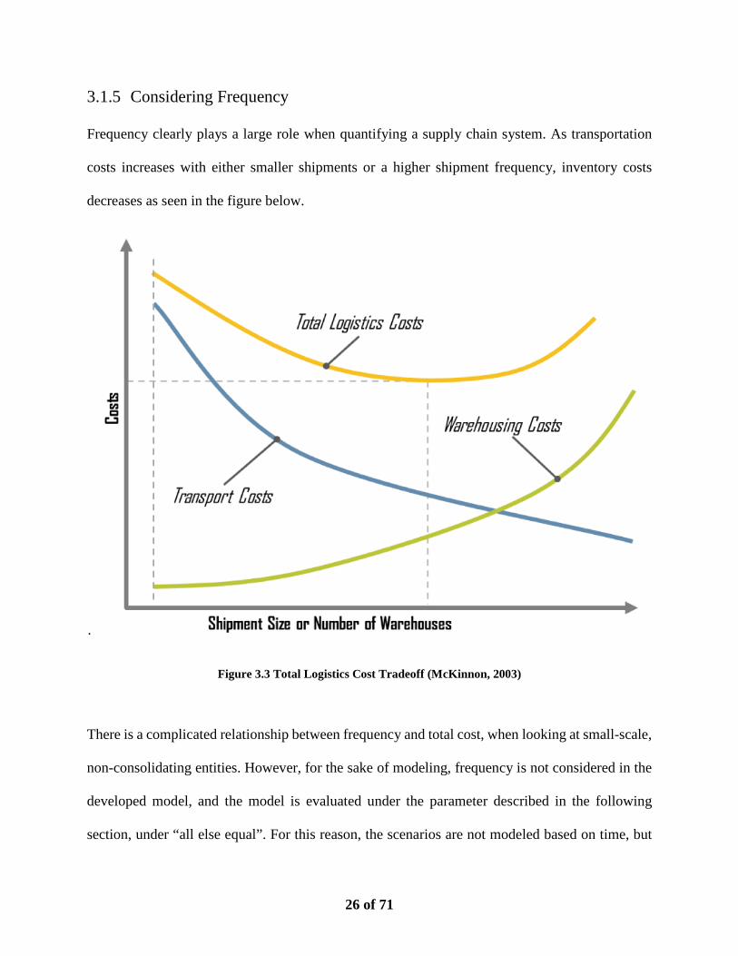
3.1.5 Considering Frequency

Frequency clearly plays a large role when quantifying a supply chain system. As transportation

costs increases with either smaller shipments or a higher shipment frequency, inventory costs

decreases as seen in the figure below.

.

Figure 3.3 Total Logistics Cost Tradeoff (McKinnon, 2003)

There is a complicated relationship between frequency and total cost, when looking at small-scale,

non-consolidating entities. However, for the sake of modeling, frequency is not considered in the

developed model, and the model is evaluated under the parameter described in the following

section, under “all else equal”. For this reason, the scenarios are not modeled based on time, but

27 of 71

as an event, and hence the impacts that are compared can be multiplied to reflect the temporal

period it covers.

3.2 ArcGIS and Network Analyst

ArcGIS is a geographic information system software application that allows the user to conduct

analysis, create, edit and use maps, compile spatial data, manage spatial and non-spatial data and

much more. It consists of a desktop application, ArcMap, supported by several integrated

applications: ArcCatalog, ArcToolbox, ArcScene and many others. It furthermore allows the user

to enable extensions, such as 3D Analyst, Spatial Analyst and Network Analyst. This project

primarily utilizes the Network Analyst Extension. It is widely used in both public and private

organizations for asset management, analysis, communication (in form of visuals and creation of

maps), and many other users.

The extension Network Analyst allows the user to create networks based on existing line works,

and through assignment of weights, routing possibilities such as dead-ends and right turns, to

model a street network, plan routes for fleets, calculate drive times and many other tasks. Network

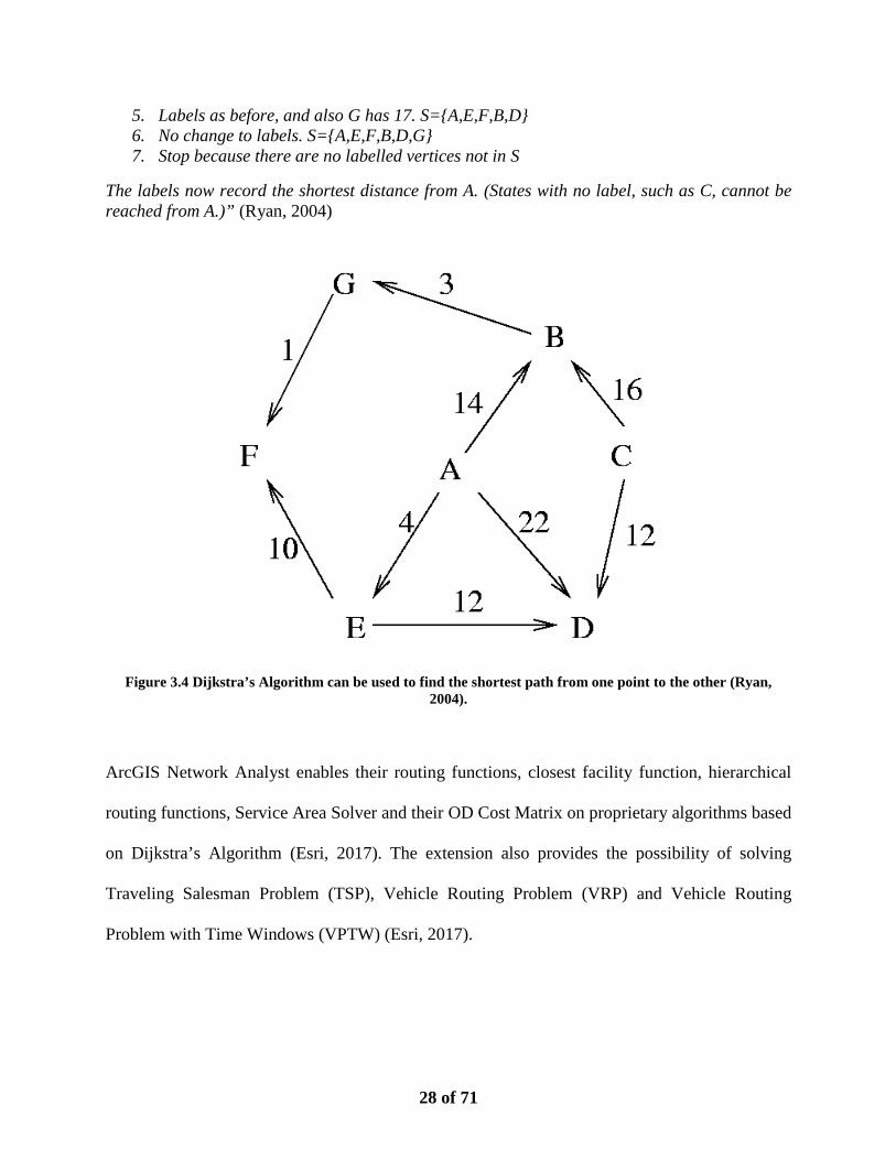
Analyst utilizes Dijkstra’s Algorithm, which calculates the length between nodes, based on current

state, and is one of the most commonly used methodologies for finding the shortest path between

two nodes. An example of the use of the algorithm can be seen in Figure 3.2 below, and is described

in the following excerpt:

“Suppose A is the source state. To explain the algorithm, we'll record the sequence of states we are in each time we get to step 4.

1. A has label 0. S = {A}. 2. A has label 0, B has 14, D has 22, E has 4. S={A,E}. 3. A is 0, B has label 14, D has been relabelled 16, F has 14. We inserted F (we could have

chosen B instead). S={A,E,F}. 4. No change to labels. S={A,E,F,B}

28 of 71

5. Labels as before, and also G has 17. S={A,E,F,B,D} 6. No change to labels. S={A,E,F,B,D,G} 7. Stop because there are no labelled vertices not in S

The labels now record the shortest distance from A. (States with no label, such as C, cannot be reached from A.)” (Ryan, 2004)

Figure 3.4 Dijkstra’s Algorithm can be used to find the shortest path from one point to the other (Ryan, 2004).

ArcGIS Network Analyst enables their routing functions, closest facility function, hierarchical

routing functions, Service Area Solver and their OD Cost Matrix on proprietary algorithms based

on Dijkstra’s Algorithm (Esri, 2017). The extension also provides the possibility of solving

Traveling Salesman Problem (TSP), Vehicle Routing Problem (VRP) and Vehicle Routing

Problem with Time Windows (VPTW) (Esri, 2017).

29 of 71

3.2.1 Modeling the Case Study

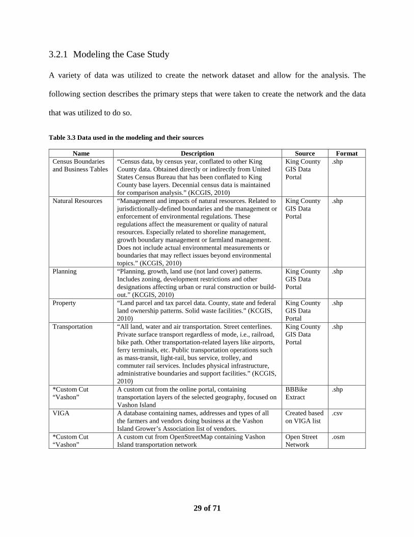
A variety of data was utilized to create the network dataset and allow for the analysis. The

following section describes the primary steps that were taken to create the network and the data

that was utilized to do so.

Table 3.3 Data used in the modeling and their sources

Name Description Source Format Census Boundaries and Business Tables

“Census data, by census year, conflated to other King County data. Obtained directly or indirectly from United States Census Bureau that has been conflated to King County base layers. Decennial census data is maintained for comparison analysis.” (KCGIS, 2010)

King County GIS Data Portal

.shp

Natural Resources “Management and impacts of natural resources. Related to jurisdictionally-defined boundaries and the management or enforcement of environmental regulations. These regulations affect the measurement or quality of natural resources. Especially related to shoreline management, growth boundary management or farmland management. Does not include actual environmental measurements or boundaries that may reflect issues beyond environmental topics.” (KCGIS, 2010)

King County GIS Data Portal

.shp

Planning “Planning, growth, land use (not land cover) patterns. Includes zoning, development restrictions and other designations affecting urban or rural construction or build-out.” (KCGIS, 2010)

King County GIS Data Portal

.shp

Property “Land parcel and tax parcel data. County, state and federal land ownership patterns. Solid waste facilities.” (KCGIS, 2010)

King County GIS Data Portal

.shp

Transportation “All land, water and air transportation. Street centerlines. Private surface transport regardless of mode, i.e., railroad, bike path. Other transportation-related layers like airports, ferry terminals, etc. Public transportation operations such as mass-transit, light-rail, bus service, trolley, and commuter rail services. Includes physical infrastructure, administrative boundaries and support facilities.” (KCGIS, 2010)

King County GIS Data Portal

.shp

*Custom Cut “Vashon”

A custom cut from the online portal, containing transportation layers of the selected geography, focused on Vashon Island

BBBike Extract

.shp

VIGA A database containing names, addresses and types of all the farmers and vendors doing business at the Vashon Island Grower’s Association list of vendors.

Created based on VIGA list

.csv

*Custom Cut “Vashon”

A custom cut from OpenStreetMap containing Vashon Island transportation network

Open Street Network

.osm

30 of 71

Establishing geography, land use and parcel data

The first step in the analysis was to create the base layer upon which the rest of the analysis is

built. Four different datasets were utilized to do so – The Census dataset, the Natural Resources

(NT) dataset, the Property dataset and the Planning dataset. The census dataset contained the

outline of the island, along with information about population and employment. This was used as

the base. Then the NT dataset were overlaid, and used to identify areas of agricultural interest. The

Planning dataset played a large role in determining the land use on the island. The full dataset

contains more than a hundred different zoning definitions, but due to the scope of the project, the

limited dataset was used, grouping the zoning definitions into 20 groups. These groups were

combined based on whether they were industrial/commercial, residential, rural or undesignated.

The parcel data provided an outline of parcels.

Creating a transportation network and a Network Dataset

Originally the King County Transportation dataset was used to create the transportation network.

One of the benefits of this network is that it contains road type information, and as this project

only required vehicular roads, that helped limit the amount of data. The datasets also included a

complete set of posted speed limits associated with one road. Network Analyst was used through

ArcCatalog to attempt to create the Network Dataset that would facilitate the analysis. However,

it was found that the Transportation dataset had some errors related to the placement and

connection of the roads. This could have been fixed through the Edit Tool, but as it produced over

100 errors that would have to be corrected manually, this was decided against. After confirming

the issue and the large amount of work required to fix it with the UW GIS libraries, OpenStreetMap

(OSM) with the BBBike Extraction Extension was instead utilized to extrapolate the street network

information. This network dataset did not have as many errors as the King County GIS dataset did,

31 of 71

but was not sorted into modes and only contained some speed information. The information about

speed limits is important, as it is utilized to construct the Network Dataset with driving times.

Therefore, the two shapefiles were joined, so that the speed limit information could be

superimposed on the OSM file. This solved some of the missing data issue. For the rest of the

missing speeds, as they were generally smaller private roads, off-roads and service roads, a speed

limit of 20 mph was assigned. This is a rough way to do it, but the scope of the work warranted it.

Working in a rural area, the posted speed limit was not decreased mathematically to an expected

speed, as would generally be done in a more urban and congested area. The length of each segment

in feet was calculated using Calculate Geometry. The Network Dataset was created using this new

shapefile, modeling turns and direction, but did not include elevation. The default evaluation

parameter chosen was drive time, created by querying “LengthOfSegment/5280*60/SpeedLimit”.

This produced the correct results for the directions, which were also selected during the modeling

of the Network Dataset. Finally, the Network Dataset with junctions was imported into ArcGIS

and tested and proved to be fully functional without any errors.

Assigning businesses and customers to network

Assigning the customers to the network was done using the Random Points tool. Prior to this,

extensive data manipulation had been taking place. Generally, randomly generated population

maps use area measurements to assign people to a given location. However, due to the low number

of expected customers – only about 60 – and the limited population and geography, this was not a

feasible option. The survey previously mentioned was used to identify where commuters who

would be interested in buying their groceries online were located within the zones previously

described. The Random Points tool allows one to, within a constraint of the zone polygon, to

randomly place points in accordance with the density of the population by zones, found in the

32 of 71

survey. To limit where these points could be placed, the layers and information from the previous

section were used, including the survey results. First, as people can live in a non-residential area,

such as an undesignated or rural zone, these three were grouped together and subtracted from the

overall dataset. The NT dataset provided information on public lands, farmland and parks, where

naturally people could not be living, and this too was erased, so that e.g. a rural area that was also

a public land, would not be included. Because of the routing analysis that would be done, and

based on the idea that if you have a parcel, then you will need a road to access it, only parcels that

were intersecting with or within 35 feet of the transportation network were carried through to the

analysis. These parcels were then dissolved into one polygon, as is required for ending up with the

correct amount of random points. This provided a final map, with some constraints on where the

random points could be placed. They were located with a requirement of a 30-foot buffer between

each house, to avoid having two points – customers – on the same parcel. All the points were

snapped to the transportation network, to facilitate routing analysis. However, these Random

Points did not have an address. It is not strictly necessary to perform the analysis, but it does make

it easier to compare locations. For this reason, a new Address Locator was created, using the Parcel

Address layer from King County as the reference and US Single House w/Sub. Then the points

were reverse geocoded to the parcels and assigned an address. Assigning businesses required less

manipulation, as VIGA carries a list of the vendors associated with their program. For the sake of

limiting the scope of the project, only farmers were included, though they also have processed and

prepared food vendors. As VIGA only shares the vendor’s names, a search tool was employed to

verify addresses. This was not possible for all the vendors, and in some cases the farms are placed

at the midpoint of a street, when their house number was not available. The .csv-file containing

33 of 71

the information was loaded into ArcGIS and the Network Analyst tool was used to locate the

addresses, using the Points.StreetAddress tool. They were then extracted to a separate feature class.

Completing the routing analysis

The ArcGIS Network Analyst tool was used to perform the network analysis. The simply Route

tool was used for most tasks, though the Incidents/Facilities tool were also used to support the

analysis. The routing points were all loaded from the previously constructed datasets, which

allowed to easily run the tool, create directions and export the data.

As with all models, the goal is to create as accurate a model as possible with the known inputs, in

cases where complete data is unavailable. Hence, this model is an approximation of what a given

scenario could look like, but there of course will always be uncertainties present.

3.3 Evaluation Criteria

The following section presents the criteria that were utilized to compare the results from the

modeling. They are separated into quantitative and qualitative criteria.

3.3.1 Quantitative Evaluation Criteria

The quantitative criteria, the reasoning and their calculation is described in the following section

and includes:

• Vehicle Miles Traveled

• Emissions

• Time in System

34 of 71

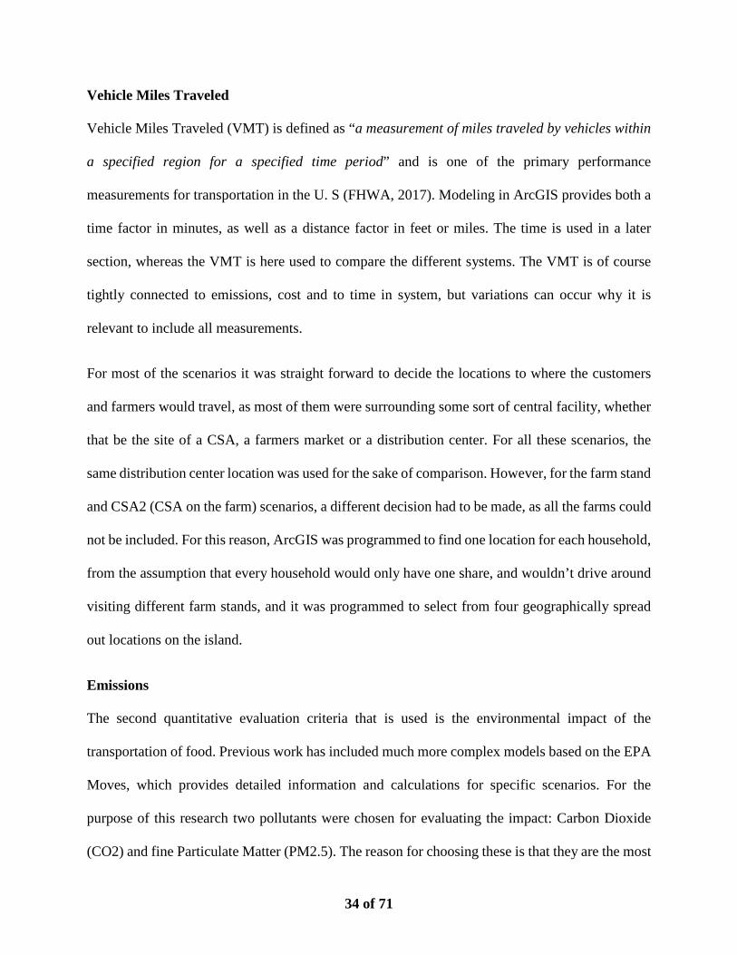
Vehicle Miles Traveled

Vehicle Miles Traveled (VMT) is defined as “a measurement of miles traveled by vehicles within

a specified region for a specified time period” and is one of the primary performance

measurements for transportation in the U. S (FHWA, 2017). Modeling in ArcGIS provides both a

time factor in minutes, as well as a distance factor in feet or miles. The time is used in a later

section, whereas the VMT is here used to compare the different systems. The VMT is of course

tightly connected to emissions, cost and to time in system, but variations can occur why it is

relevant to include all measurements.

For most of the scenarios it was straight forward to decide the locations to where the customers

and farmers would travel, as most of them were surrounding some sort of central facility, whether

that be the site of a CSA, a farmers market or a distribution center. For all these scenarios, the

same distribution center location was used for the sake of comparison. However, for the farm stand

and CSA2 (CSA on the farm) scenarios, a different decision had to be made, as all the farms could

not be included. For this reason, ArcGIS was programmed to find one location for each household,

from the assumption that every household would only have one share, and wouldn’t drive around

visiting different farm stands, and it was programmed to select from four geographically spread

out locations on the island.

Emissions

The second quantitative evaluation criteria that is used is the environmental impact of the

transportation of food. Previous work has included much more complex models based on the EPA

Moves, which provides detailed information and calculations for specific scenarios. For the

purpose of this research two pollutants were chosen for evaluating the impact: Carbon Dioxide

(CO2) and fine Particulate Matter (PM2.5). The reason for choosing these is that they are the most

35 of 71

commonly compared pollutants, and together give a reasonable picture of both local and global

impacts of emissions. Furthermore, the gasoline consumption is listed for comparison.

Table 3.4 Emissions and Fuel Consumption for Passenger Cars (EPA, 2005)

Pollutant/Fuel Emission and Fuel Consumption Rates (Per Mile Drive)

Calculation

Particulate Matter (PM2.5) 0.0049 g 0.0049 g /mi * miles/year * 1 lb./454 g

Carbon Dioxide (CO2) 369 g 369 g /mi * miles/year * 1 lb./454 g Gasoline Consumption 0.0417 gallons (gal) miles/year / mpg

These numbers are slightly different for light duty trucks. For all the non-customer movements, it

is assumed that it is a light duty truck that is in use. The emission details for light duty trucks can

be seen in the table below.

Table 3.5 Emissions and Fuel Consumption for Light-Duty Trucks * (EPA, 2005) Pollutant/Fuel Emission and Fuel Consumption Rates

(Per Mile Drive) Calculation

Particulate Matter (PM2.5) 0.0060 g 0.0060 g /mi * miles/year * 1 lb./454 g

Carbon Dioxide (CO2) 511 g 511 g /mi * miles/year * 1 lb./454 g Gasoline Consumption 0.0578 gallons (gal) miles/year / mpg

* Most pick-up trucks, SUVs etc.

The tables above require knowledge of the fuel economy of the cars in use. For this study, it was

assumed that customers would all be driving passenger cars, and farmers and VF would all be

driving light trucks. The table below shows the average gas mileage for new cars by type and year.

In 2014 a study found that both the average passenger car and the average light duty truck is 11.4

years old these calculations assume 2005-mileage (IHS, 2014). According to the EPA, the average

car on the road today has a fuel economy of 21.6 miles per gallon. This fits well with the estimate

for new light trucks in 2005, but this does include both large trucks and small two-person cars. It

does however confirm that the 2005 estimates in the table below are reasonable to use for modeling

purposes.

36 of 71

Table 3.6 Average Fuel Efficiency of U.S. Light Duty Vehicles (USDOT, 2014) 2000 2001 2002 2003 2004 2005 2006 2007 2008 2009 2010

Passenger car 28.5 28.8 29 29.5 29.5 30.3 30.1 31.2 31.5 32.9 33.9 Light truck (<8,500 lbs. GVWR)

21.3 20.9 21.4 21.8 21.5 22.1 22.5 23.1 23.6 24.8 25.2

Time in System

The Time in System evaluation criteria seeks to describe the amount of time that the produce will

spent under less than optimal conditions. As previously discussed, food needs to be kept under

specific temperatures and has higher requirements of packaging, transportation and care to avoid

decreasing the quality and therefore the value of the produce. One of the most important aspects

to customers who select local produce over non-local produce, is the perceived freshness of the

product, why Time in System becomes a proxy that describes the freshness of the available

produce. For modeling purposes, it is assumed that the produce is stored under optimal conditions

both before it begins its trip; at the farms where the produce originated from, and after it ends its

trip; at the customers who bought the produce’s homes. It is also assumed that when it is kept at

the central distribution facility, it is kept under optimal conditions. Because transportation of

produce is one of the more strenuous, and potentially damaging things that produce goes through,

the time spent on the road is considered Time in System. This is captured through modeling by

calculating DriveTime for each scenario. The specific assumptions for the remaining Time in

System components are described in the individual sections.

𝑻𝑻𝑻𝑻𝑻𝑻𝑻𝑻 𝑻𝑻𝒊𝒊 𝑺𝑺𝑺𝑺𝑺𝑺𝑺𝑺𝑻𝑻𝑻𝑻 = 𝑫𝑫𝑫𝑫𝑻𝑻𝑫𝑫𝑻𝑻𝑻𝑻𝑻𝑻𝑻𝑻𝑻𝑻𝑫𝑫 + 𝑫𝑫𝑫𝑫𝑻𝑻𝑫𝑫𝑻𝑻𝑻𝑻𝑻𝑻𝑻𝑻𝑻𝑻𝑫𝑫 + 𝑺𝑺𝑺𝑺𝑺𝑺𝑫𝑫𝑺𝑺𝑺𝑺𝑻𝑻𝑻𝑻𝑻𝑻𝑻𝑻𝑻𝑻𝑫𝑫

(3-1)

When something is stored for several hours, and sold at regular intervals all throughout this time,

the item sold will have had varying time in storage, depending on when the item was sold and left

37 of 71

storage. To capture the fact that some produce will have had minimal time in storage, and some

produce may have had spent all its time in storage, the time in storage is divided by two for all

scenarios, to get the average StorageTime. To capture the cost of transferring produce between

two stages, a penalty was added for changes e.g. between a being on the farm and being at a

distribution center. This penalty changes based on scenario, and is described further in the

comparisons of the different scenarios, but incurs 60 minutes every time the produce is moved

between a storage location (farms, distribution center, customers), to also capture the degradation

in quality from handling.

3.3.2 Qualitative Considerations

This section describes the two qualitative measurements that was included as part of the evaluation

of the different scenarios. The criteria include:

• Accessibility

• Community

Accessibility

Accessibility covers the possibilities and lack thereof that customers have of accessing the produce

in each scenario. If a scenario requires the user to own a car to drive to the location, the accessibility

is clearly lower than in a scenario where the produce is delivered to the customer. This could have

been quantified through spatial analysis, but this was not done for the purposes of this research.

Access also increases when a product can be obtained at a location that is more central to the

consumer; requires the consumer to drive a shorter distance, or; is closer to a high-level

transportation network, such as an arterial or ferry, as opposed to located on a local, low-speed

road.

38 of 71

Community

As discussed in Chapter 2, the notion of community and connectedness is important to many of

the users who choose to shop at farmers markets and similar initiatives. This was not modeled or

quantified in any way in the research at hand, but is discussed as part of the different scenarios.

Community increases when the interaction allows for interaction between the producer and the

end-consumer; allows the consumer to learn about the produce they’re obtaining; or allows either

part to be present or participate in their local community in any way.

39 of 71

4. ANALYSIS AND RESULTS

The following section presents the analysis that was completed based on the methodology

presented in the previous section. For all scenarios the relating maps are included in Appendix A.

All of the scenarios are to some extent similar in terms of their routing, and can therefore be shown

as a combination of the following maps. Section 4.1 and Section 4.2 contain references to the maps

that the given scenarios are constructed and calculated from.

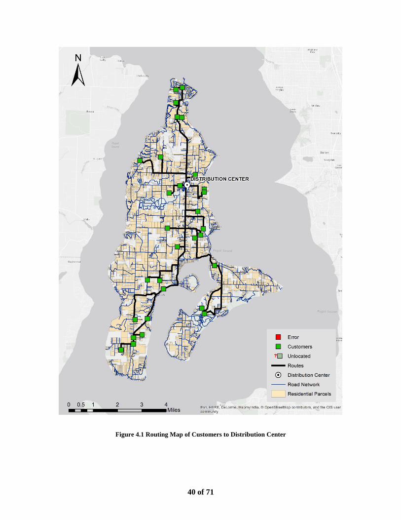
40 of 71

Figure 4.1 Routing Map of Customers to Distribution Center

41 of 71

Figure 4.2 Routing Map of Farmers to Distribution Center

42 of 71

Figure 4.3 Routing Map of Customers to Individual Farms

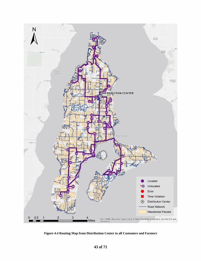
43 of 71

Figure 4.4 Routing Map from Distribution Center to all Customers and Farmers

44 of 71

Figure 4.5 Routing Map of Roundtrip from Farmers to Distribution Center

45 of 71

Figure 4.6 Routing Map of Roundtrip from Customers to Distribution Center

46 of 71

4.1 Analysis of Baseline Scenarios

The following section describes the results obtained from the modeling regarding the baseline

scenarios. The codes used to identify the various scenarios are as follows:

Table 4.1 Baseline Scenarios ID DC DC DESCRIPTION ACRONYM MEANING MAPS

B1-FM

Farmers Customers Farmers drive to the Farmers Market, where to customers also drive to buy produce

Baseline 1 Farmer’s Market 4.1, 4.2

B2-CSA1

Farmers Customers Farmers will deliver produce to a central location, where it will be packed and picked up by customers

Baseline 2 Community Supported Agriculture 1

4.1, 4.2

B3-CSA2

N/A Customers Customers drive to individual farms. Produce stays on farm.

Baseline 3 Community Supported Agriculture 2

4.3

B4-FS

N/A Customers Like CSA2, this solution has customers drive to individual farms to purchase produce

Baseline 4 Farm Stand 4.3

4.1.1 VMT

The results of the analysis with regards to VMT is presented in the following:

Table 4.2 VMT and DriveTime for the Baseline Scenarios ID DC VMT DC DC VMT (mi) Total VMT (mi)

B1-FM Farmers 166.6 Customers 246.6 413.2 B2-CSA1 Farmers 166.6 Customers 246.6 413.2 B3-CSA2 N/A 0 Customers 264.2 264.2 B4-FS N/A 0 Customers 264.2 264.2

The total VMT for the baseline scenarios came out to 413.1 miles for scenarios B1 and B2, and

264.2 miles for scenarios B3 and B4. It was expected that B3 and B4 would have an overall lower

total VMT. Remembering the (Coley, et al., 2008) paper, which found that driving more than 6.7

kilometers or 4.2 miles round trip to pick up produce would likely result in a negative total impact

on the environment, these results are both more than 4.2 miles on average. With a total of 30

customers, the roundtrip mileage for scenario B1 and B2 is 8.22 miles and for scenario B3 and B4

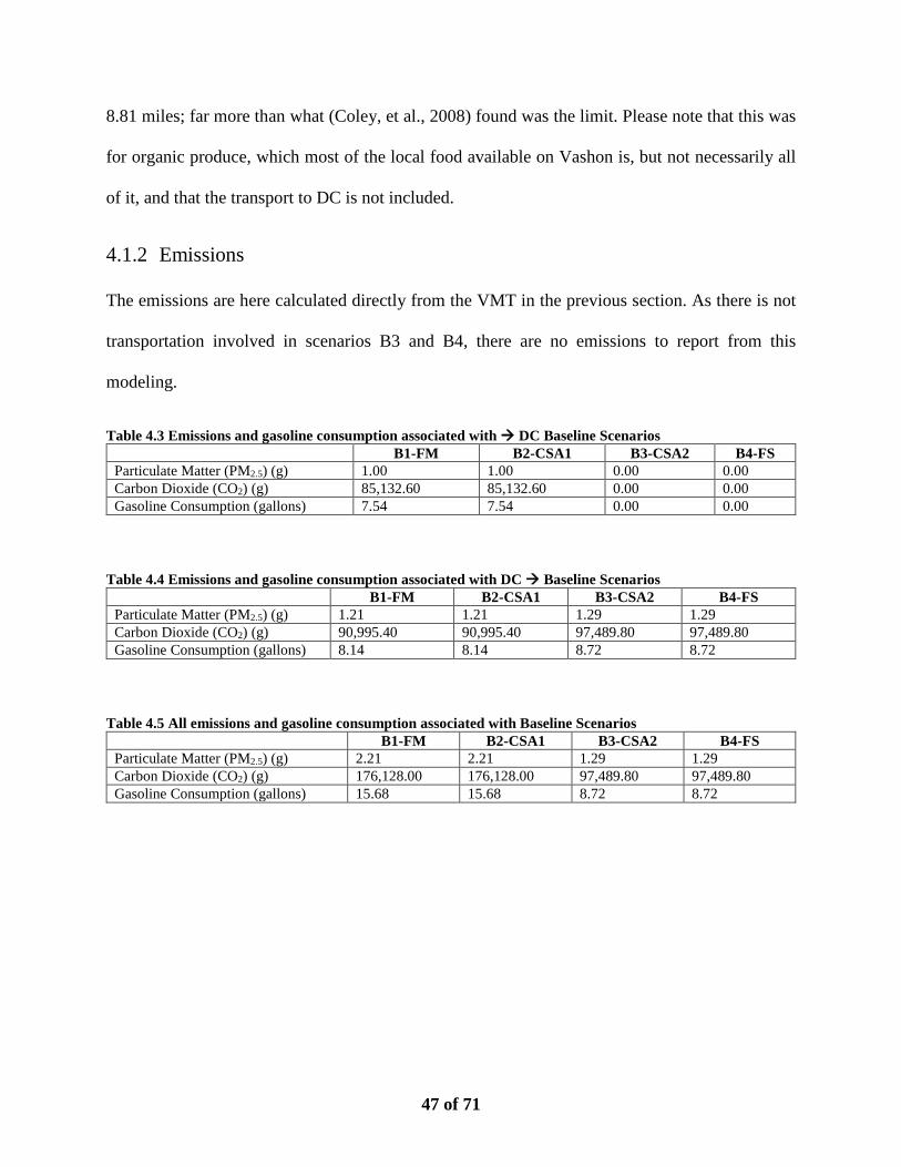
47 of 71

8.81 miles; far more than what (Coley, et al., 2008) found was the limit. Please note that this was

for organic produce, which most of the local food available on Vashon is, but not necessarily all

of it, and that the transport to DC is not included.

4.1.2 Emissions

The emissions are here calculated directly from the VMT in the previous section. As there is not

transportation involved in scenarios B3 and B4, there are no emissions to report from this

modeling.

Table 4.3 Emissions and gasoline consumption associated with DC Baseline Scenarios B1-FM B2-CSA1 B3-CSA2 B4-FS

Particulate Matter (PM2.5) (g) 1.00 1.00 0.00 0.00 Carbon Dioxide (CO2) (g) 85,132.60 85,132.60 0.00 0.00 Gasoline Consumption (gallons) 7.54 7.54 0.00 0.00

Table 4.4 Emissions and gasoline consumption associated with DC Baseline Scenarios B1-FM B2-CSA1 B3-CSA2 B4-FS

Particulate Matter (PM2.5) (g) 1.21 1.21 1.29 1.29 Carbon Dioxide (CO2) (g) 90,995.40 90,995.40 97,489.80 97,489.80 Gasoline Consumption (gallons) 8.14 8.14 8.72 8.72

Table 4.5 All emissions and gasoline consumption associated with Baseline Scenarios B1-FM B2-CSA1 B3-CSA2 B4-FS

Particulate Matter (PM2.5) (g) 2.21 2.21 1.29 1.29 Carbon Dioxide (CO2) (g) 176,128.00 176,128.00 97,489.80 97,489.80 Gasoline Consumption (gallons) 15.68 15.68 8.72 8.72

48 of 71

Figure 4.7 Relative comparison of emissions and gasoline consumption between the four scenarios

In line with the results for the VMT, the emissions total is higher for the first two scenarios than

for the last two scenarios.

4.1.3 Time in System

The Time in System calculations were determined as follows, and all divided by two as described

in section 3.3.1:

B1-FM: For the Farmers Market scenario, the current operating hours for the Vashon Fresh

Farmers Market is between 10am and 2pm, giving a total operating time of 4 hours or 240 minutes.

Looking at nearby Farmers Markets, it seems like this is a common operating time for farmers

markets: U-District (9am-2pm, 5 hours); Capitol Hill Broadway (11am-3pm, 4 hours); West

Seattle, Magnolia (10am-2pm, 4 hours); Lake City, Columbia City (3pm-7pm, 4 hours).

For the transfer between the farm and the distribution center, a one hour time penalty is incurred,

and for the transfer between the DC and the customer another hours is.

0

0.2

0.4

0.6

0.8

1

1.2

Particulate Matter (PM2.5) (g) Carbon Dioxide (CO2) (g) Gasoline Consumption (gallons)

Relative emissions and gasoline consumption

B1-FM B2-CSA1 B3-CSA2 B4-FS

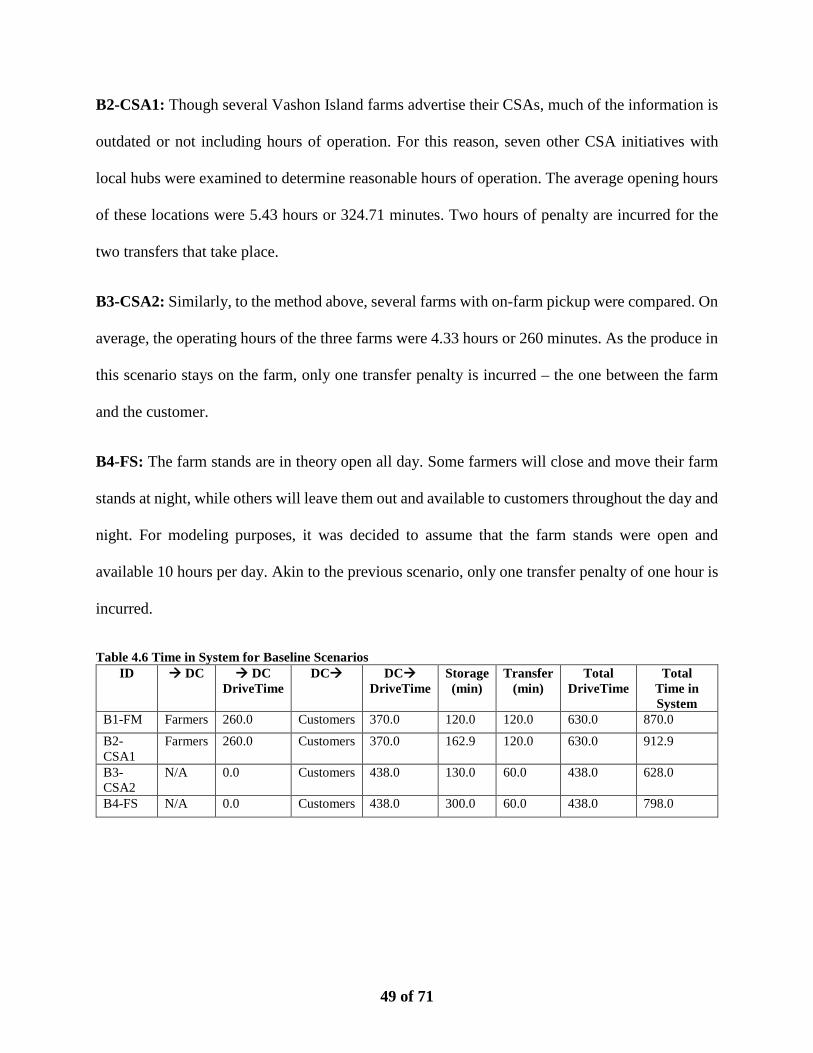
49 of 71

B2-CSA1: Though several Vashon Island farms advertise their CSAs, much of the information is

outdated or not including hours of operation. For this reason, seven other CSA initiatives with

local hubs were examined to determine reasonable hours of operation. The average opening hours

of these locations were 5.43 hours or 324.71 minutes. Two hours of penalty are incurred for the

two transfers that take place.

B3-CSA2: Similarly, to the method above, several farms with on-farm pickup were compared. On

average, the operating hours of the three farms were 4.33 hours or 260 minutes. As the produce in

this scenario stays on the farm, only one transfer penalty is incurred – the one between the farm

and the customer.

B4-FS: The farm stands are in theory open all day. Some farmers will close and move their farm

stands at night, while others will leave them out and available to customers throughout the day and

night. For modeling purposes, it was decided to assume that the farm stands were open and

available 10 hours per day. Akin to the previous scenario, only one transfer penalty of one hour is

incurred.

Table 4.6 Time in System for Baseline Scenarios ID DC DC

DriveTime DC DC

DriveTime Storage (min)

Transfer (min)

Total DriveTime

Total Time in System

B1-FM Farmers 260.0 Customers 370.0 120.0 120.0 630.0 870.0 B2-CSA1

Farmers 260.0 Customers 370.0 162.9 120.0 630.0 912.9

B3-CSA2

N/A 0.0 Customers 438.0 130.0 60.0 438.0 628.0

B4-FS N/A 0.0 Customers 438.0 300.0 60.0 438.0 798.0

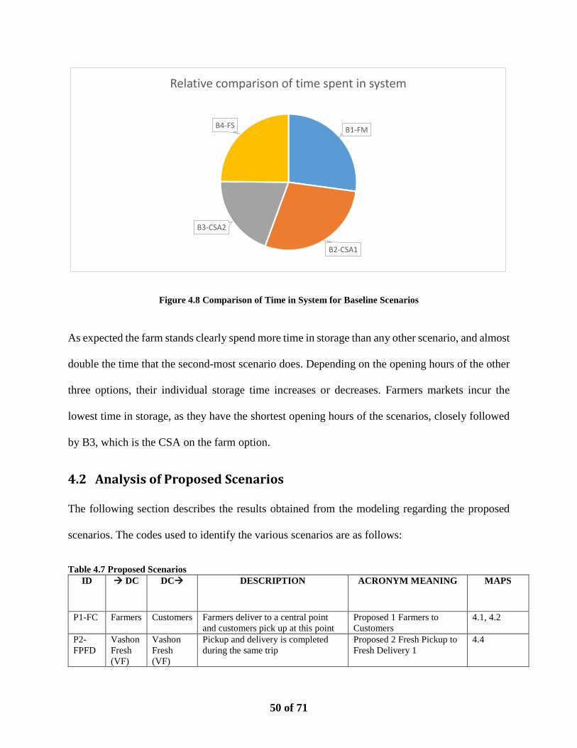
50 of 71

Figure 4.8 Comparison of Time in System for Baseline Scenarios

As expected the farm stands clearly spend more time in storage than any other scenario, and almost

double the time that the second-most scenario does. Depending on the opening hours of the other

three options, their individual storage time increases or decreases. Farmers markets incur the

lowest time in storage, as they have the shortest opening hours of the scenarios, closely followed

by B3, which is the CSA on the farm option.

4.2 Analysis of Proposed Scenarios

The following section describes the results obtained from the modeling regarding the proposed

scenarios. The codes used to identify the various scenarios are as follows:

Table 4.7 Proposed Scenarios ID DC DC DESCRIPTION ACRONYM MEANING MAPS

P1-FC Farmers Customers Farmers deliver to a central point and customers pick up at this point

Proposed 1 Farmers to Customers

4.1, 4.2

P2-FPFD

Vashon Fresh (VF)

Vashon Fresh (VF)

Pickup and delivery is completed during the same trip

Proposed 2 Fresh Pickup to Fresh Delivery 1

4.4

B1-FM

B2-CSA1

B3-CSA2

B4-FS

Relative comparison of time spent in system

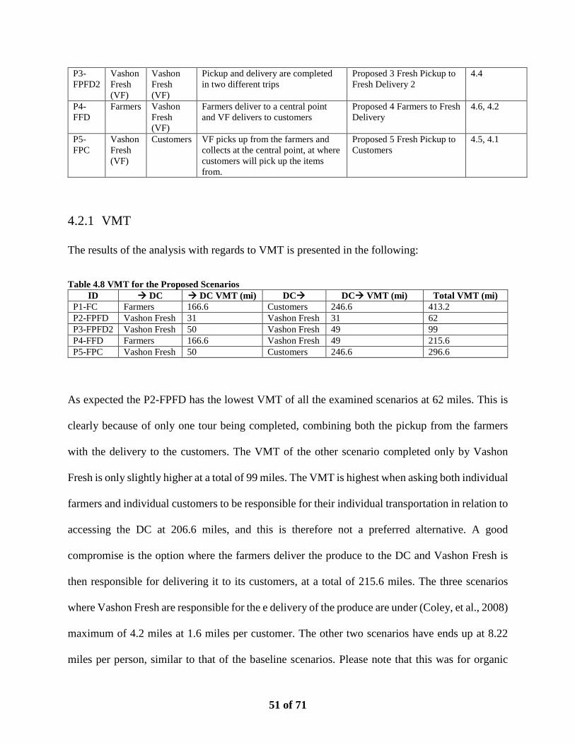
51 of 71

P3-FPFD2

Vashon Fresh (VF)

Vashon Fresh (VF)

Pickup and delivery are completed in two different trips

Proposed 3 Fresh Pickup to Fresh Delivery 2

4.4

P4-FFD

Farmers Vashon Fresh (VF)

Farmers deliver to a central point and VF delivers to customers

Proposed 4 Farmers to Fresh Delivery

4.6, 4.2

P5-FPC

Vashon Fresh (VF)

Customers VF picks up from the farmers and collects at the central point, at where customers will pick up the items from.

Proposed 5 Fresh Pickup to Customers

4.5, 4.1

4.2.1 VMT

The results of the analysis with regards to VMT is presented in the following:

Table 4.8 VMT for the Proposed Scenarios ID DC DC VMT (mi) DC DC VMT (mi) Total VMT (mi)

P1-FC Farmers 166.6 Customers 246.6 413.2 P2-FPFD Vashon Fresh 31 Vashon Fresh 31 62 P3-FPFD2 Vashon Fresh 50 Vashon Fresh 49 99 P4-FFD Farmers 166.6 Vashon Fresh 49 215.6 P5-FPC Vashon Fresh 50 Customers 246.6 296.6

As expected the P2-FPFD has the lowest VMT of all the examined scenarios at 62 miles. This is

clearly because of only one tour being completed, combining both the pickup from the farmers

with the delivery to the customers. The VMT of the other scenario completed only by Vashon

Fresh is only slightly higher at a total of 99 miles. The VMT is highest when asking both individual

farmers and individual customers to be responsible for their individual transportation in relation to

accessing the DC at 206.6 miles, and this is therefore not a preferred alternative. A good

compromise is the option where the farmers deliver the produce to the DC and Vashon Fresh is

then responsible for delivering it to its customers, at a total of 215.6 miles. The three scenarios

where Vashon Fresh are responsible for the e delivery of the produce are under (Coley, et al., 2008)

maximum of 4.2 miles at 1.6 miles per customer. The other two scenarios have ends up at 8.22

miles per person, similar to that of the baseline scenarios. Please note that this was for organic

52 of 71

produce, which most of the local food available on Vashon is, but not necessarily all of it, and that

the transport to DC is not included.

4.2.2 Emissions

The emissions are here calculated directly from the VMT in the previous section.

Table 4.9 Emissions and gasoline consumption associated with DC Proposed Scenarios P1-FC P2-FPFD P3-FPFD2 P4-FFD P5-FPC

Particulate Matter (PM2.5) (g) 1.0 0.2 0.3 1.0 0.3 Carbon Dioxide (CO2) (g) 85,132.6 15,841.0 25,550.0 85,132.6 25,550.0 Gasoline Consumption (gallons) 7.5 1.4 2.3 7.5 2.3 Sum 88,229.3 16,417.2 26,479.4 88,229.3 26,479.4

Table 4.10 Emissions and gasoline consumption associated with DC Proposed Scenarios

From DC

P1-FC P2-FPFD P3-FPFD2 P4-FFD P5-FPC

Particulate Matter (PM2.5) (g) 1.2 0.2 0.3 0.3 1.2 Carbon Dioxide (CO2) (g) 90,995.4 15,841.0 25,039.0 25,039.0 90,995.4 Gasoline Consumption (gallons) 8.1 1.4 2.2 2.2 8.1

Table 4.11 All emissions and gasoline consumption associated with Proposed Scenarios

P1-FC P2-FPFD P3-FPFD2 P4-FFD P5-FPC Particulate Matter (PM2.5) (g) 2.2 0.4 0.6 1.3 1.5 Carbon Dioxide (CO2) (g) 176,128.0 31,682.0 50,589.0 110,171.6 116,545.4 Gasoline Consumption (gallons) 15.7 2.8 4.5 9.8 10.4

Figure 4.9 Relative Comparison of Pollutants and Gasoline Consumption

0

0.2

0.4

0.6

0.8

1

1.2

Particulate Matter (PM2.5) (g) Carbon Dioxide (CO2) (g) Gasoline Consumption (gallons)

Relative Comparison of Proposed Scenarios

P1-FC P2-FPFD P3-FPFD2 P4-FFD P5-FPC

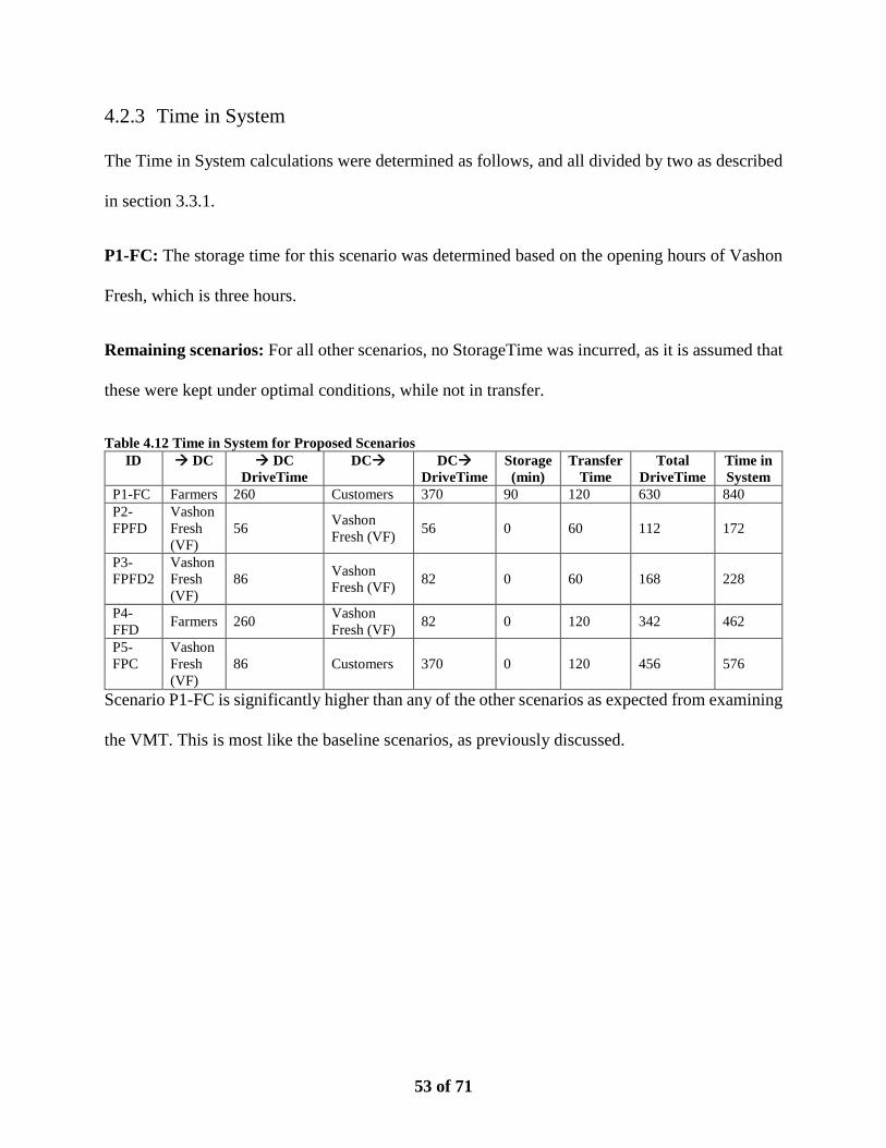
53 of 71

4.2.3 Time in System

The Time in System calculations were determined as follows, and all divided by two as described

in section 3.3.1.

P1-FC: The storage time for this scenario was determined based on the opening hours of Vashon

Fresh, which is three hours.

Remaining scenarios: For all other scenarios, no StorageTime was incurred, as it is assumed that

these were kept under optimal conditions, while not in transfer.

Table 4.12 Time in System for Proposed Scenarios ID DC DC

DriveTime DC DC

DriveTime Storage (min)

Transfer Time

Total DriveTime

Time in System

P1-FC Farmers 260 Customers 370 90 120 630 840 P2-FPFD

Vashon Fresh (VF)

56 Vashon Fresh (VF) 56 0 60 112 172

P3-FPFD2

Vashon Fresh (VF)

86 Vashon Fresh (VF) 82 0 60 168 228

P4-FFD Farmers 260 Vashon

Fresh (VF) 82 0 120 342 462

P5-FPC

Vashon Fresh (VF)

86 Customers 370 0 120 456 576

Scenario P1-FC is significantly higher than any of the other scenarios as expected from examining

the VMT. This is most like the baseline scenarios, as previously discussed.

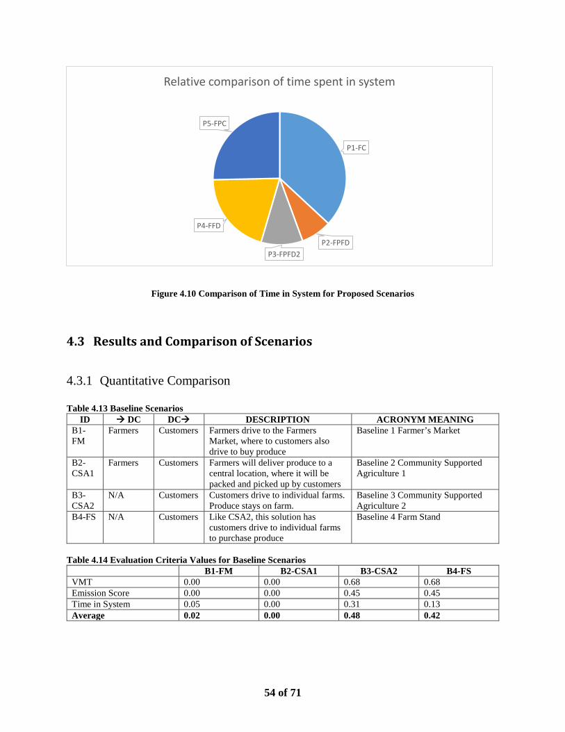
54 of 71

Figure 4.10 Comparison of Time in System for Proposed Scenarios

4.3 Results and Comparison of Scenarios

4.3.1 Quantitative Comparison

Table 4.13 Baseline Scenarios ID DC DC DESCRIPTION ACRONYM MEANING

B1-FM

Farmers Customers Farmers drive to the Farmers Market, where to customers also drive to buy produce

Baseline 1 Farmer’s Market

B2-CSA1

Farmers Customers Farmers will deliver produce to a central location, where it will be packed and picked up by customers

Baseline 2 Community Supported Agriculture 1

B3-CSA2

N/A Customers Customers drive to individual farms. Produce stays on farm.

Baseline 3 Community Supported Agriculture 2

B4-FS N/A Customers Like CSA2, this solution has customers drive to individual farms to purchase produce

Baseline 4 Farm Stand

Table 4.14 Evaluation Criteria Values for Baseline Scenarios

B1-FM B2-CSA1 B3-CSA2 B4-FS VMT 0.00 0.00 0.68 0.68 Emission Score 0.00 0.00 0.45 0.45 Time in System 0.05 0.00 0.31 0.13 Average 0.02 0.00 0.48 0.42

P1-FC

P2-FPFDP3-FPFD2

P4-FFD

P5-FPC

Relative comparison of time spent in system

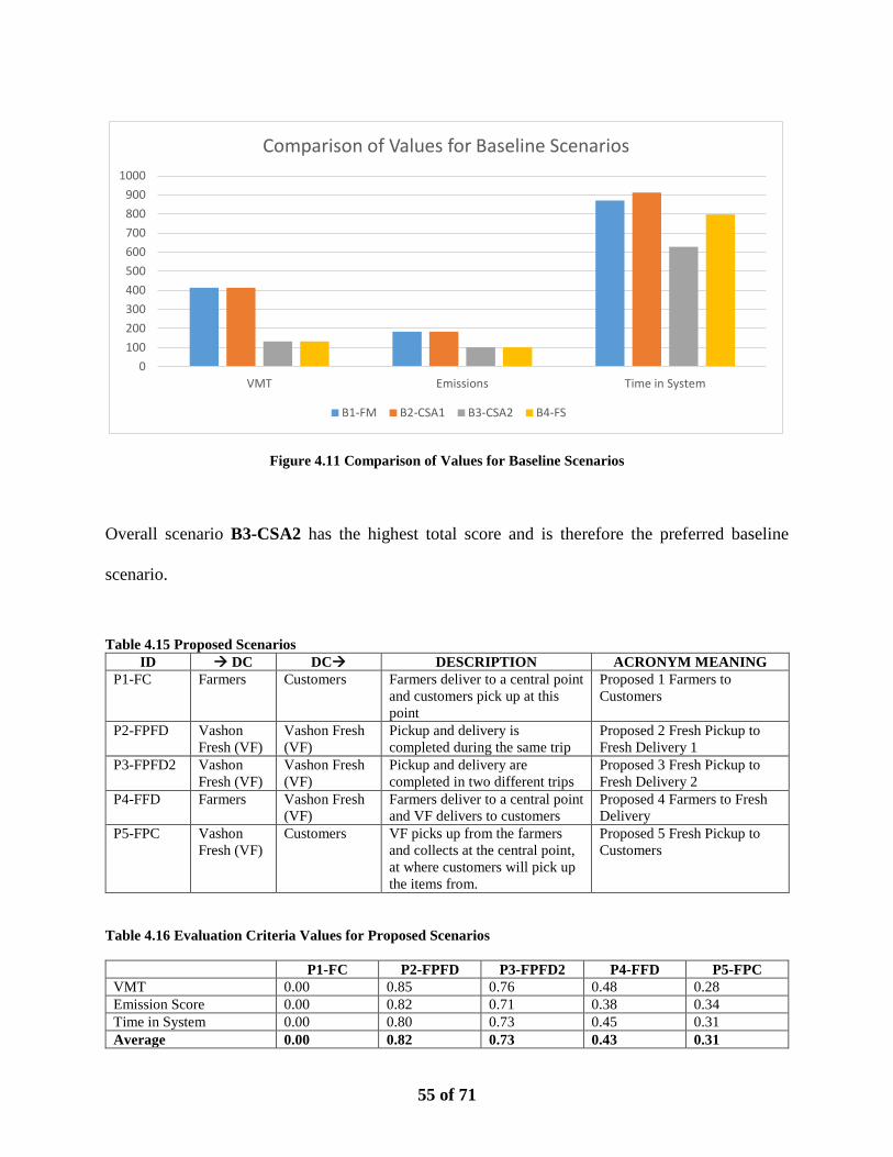
55 of 71

Figure 4.11 Comparison of Values for Baseline Scenarios

Overall scenario B3-CSA2 has the highest total score and is therefore the preferred baseline

scenario.

Table 4.15 Proposed Scenarios

ID DC DC DESCRIPTION ACRONYM MEANING P1-FC Farmers Customers Farmers deliver to a central point

and customers pick up at this point

Proposed 1 Farmers to Customers

P2-FPFD Vashon Fresh (VF)

Vashon Fresh (VF)

Pickup and delivery is completed during the same trip

Proposed 2 Fresh Pickup to Fresh Delivery 1

P3-FPFD2 Vashon Fresh (VF)

Vashon Fresh (VF)

Pickup and delivery are completed in two different trips

Proposed 3 Fresh Pickup to Fresh Delivery 2

P4-FFD Farmers Vashon Fresh (VF)

Farmers deliver to a central point and VF delivers to customers

Proposed 4 Farmers to Fresh Delivery

P5-FPC Vashon Fresh (VF)

Customers VF picks up from the farmers and collects at the central point, at where customers will pick up the items from.

Proposed 5 Fresh Pickup to Customers

Table 4.16 Evaluation Criteria Values for Proposed Scenarios

P1-FC P2-FPFD P3-FPFD2 P4-FFD P5-FPC VMT 0.00 0.85 0.76 0.48 0.28 Emission Score 0.00 0.82 0.71 0.38 0.34 Time in System 0.00 0.80 0.73 0.45 0.31 Average 0.00 0.82 0.73 0.43 0.31

0100200300400500600700800900

1000

VMT Emissions Time in System

Comparison of Values for Baseline Scenarios

B1-FM B2-CSA1 B3-CSA2 B4-FS

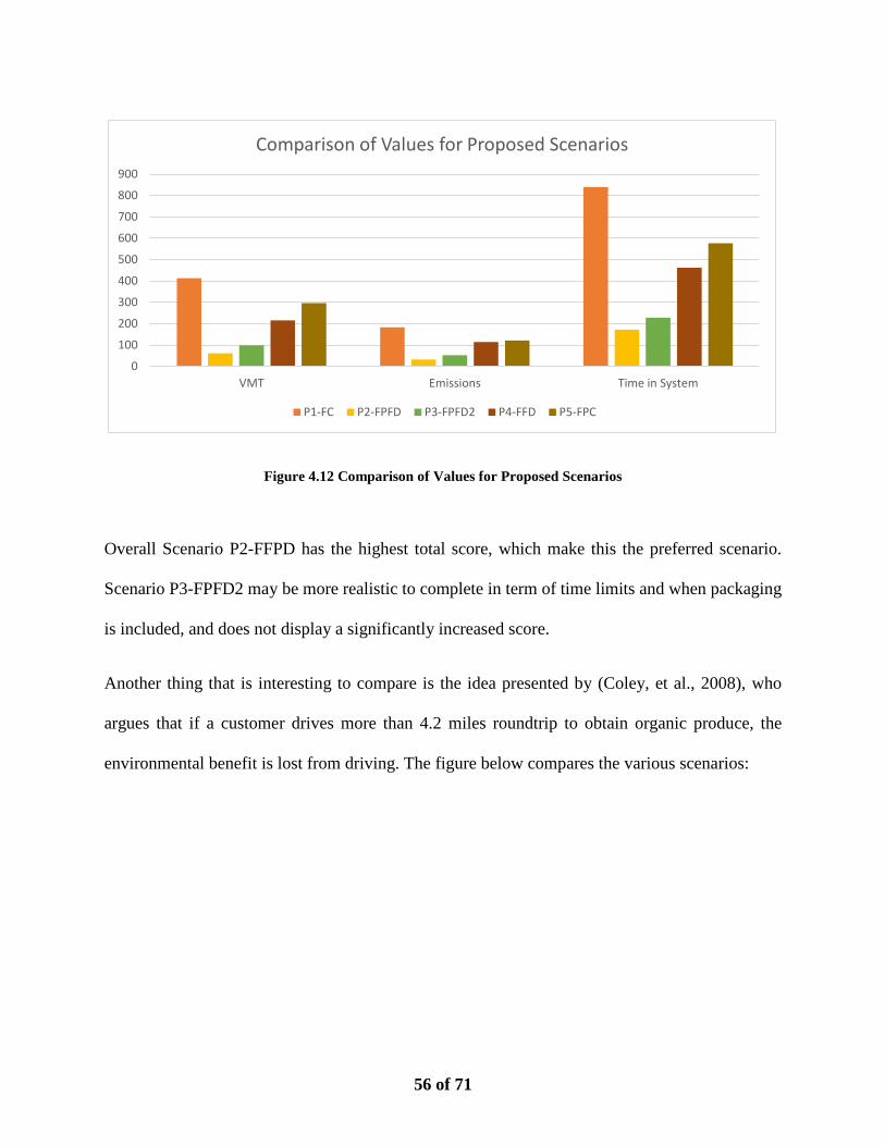
56 of 71

Figure 4.12 Comparison of Values for Proposed Scenarios

Overall Scenario P2-FFPD has the highest total score, which make this the preferred scenario.

Scenario P3-FPFD2 may be more realistic to complete in term of time limits and when packaging

is included, and does not display a significantly increased score.

Another thing that is interesting to compare is the idea presented by (Coley, et al., 2008), who

argues that if a customer drives more than 4.2 miles roundtrip to obtain organic produce, the

environmental benefit is lost from driving. The figure below compares the various scenarios:

0

100

200

300

400

500

600

700

800

900

VMT Emissions Time in System

Comparison of Values for Proposed Scenarios

P1-FC P2-FPFD P3-FPFD2 P4-FFD P5-FPC

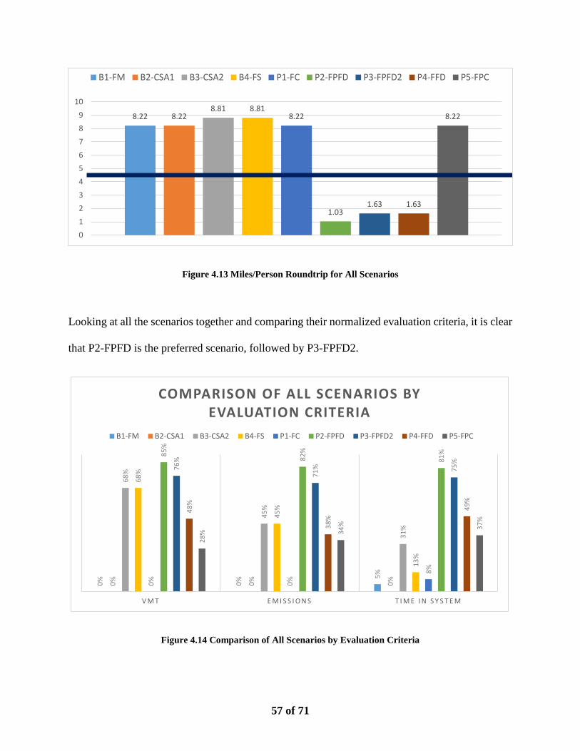
57 of 71

Figure 4.13 Miles/Person Roundtrip for All Scenarios

Looking at all the scenarios together and comparing their normalized evaluation criteria, it is clear

that P2-FPFD is the preferred scenario, followed by P3-FPFD2.

Figure 4.14 Comparison of All Scenarios by Evaluation Criteria

8.22 8.228.81 8.81

8.22

1.031.63 1.63

8.22

0123456789

10

B1-FM B2-CSA1 B3-CSA2 B4-FS P1-FC P2-FPFD P3-FPFD2 P4-FFD P5-FPC

0% 0%

5%

0% 0% 0%

68%

45%

31%

68%

45%

13%

0% 0%

8%

85%

82%

81%

76%

71% 75

%

48%

38%

49%

28% 34

% 37%

V M T E M I S S I O N S T I M E I N S Y S T E M

COMPARISON OF ALL SCENARIOS BY EVALUATION CRITERIA

B1-FM B2-CSA1 B3-CSA2 B4-FS P1-FC P2-FPFD P3-FPFD2 P4-FFD P5-FPC

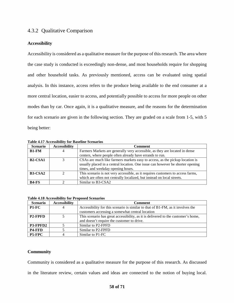
58 of 71

4.3.2 Qualitative Comparison

Accessibility

Accessibility is considered as a qualitative measure for the purpose of this research. The area where

the case study is conducted is exceedingly non-dense, and most households require for shopping

and other household tasks. As previously mentioned, access can be evaluated using spatial

analysis. In this instance, access refers to the produce being available to the end consumer at a

more central location, easier to access, and potentially possible to access for more people on other

modes than by car. Once again, it is a qualitative measure, and the reasons for the determination

for each scenario are given in the following section. They are graded on a scale from 1-5, with 5

being better:

Table 4.17 Accessibility for Baseline Scenarios Scenario Accessibility Comment

B1-FM 4 Farmers Markets are generally very accessible, as they are located in dense centers, where people often already have errands to run.

B2-CSA1 3 CSAs are much like farmers markets easy to access, as the pickup location is usually placed in a central location. One issue can however be shorter opening times, and weekday opening hours.

B3-CSA2 2 This scenario is not very accessible, as it requires customers to access farms, which are often not centrally localized, but instead on local streets.

B4-FS 2 Similar to B3-CSA2

Table 4.18 Accessibility for Proposed Scenarios Scenario Accessibility Comment

P1-FC 4 Accessibility for this scenario is similar to that of B1-FM, as it involves the customers accessing a somewhat central location

P2-FPFD 5 This scenario has great accessibility, as it is delivered to the customer’s home, and doesn’t require the customer to drive.

P3-FPFD2 5 Similar to P2-FPFD P4-FFD 5 Similar to P2-FPFD P5-FPC 4 Similar to P1-FC

Community

Community is considered as a qualitative measure for the purpose of this research. As discussed

in the literature review, certain values and ideas are connected to the notion of buying local.

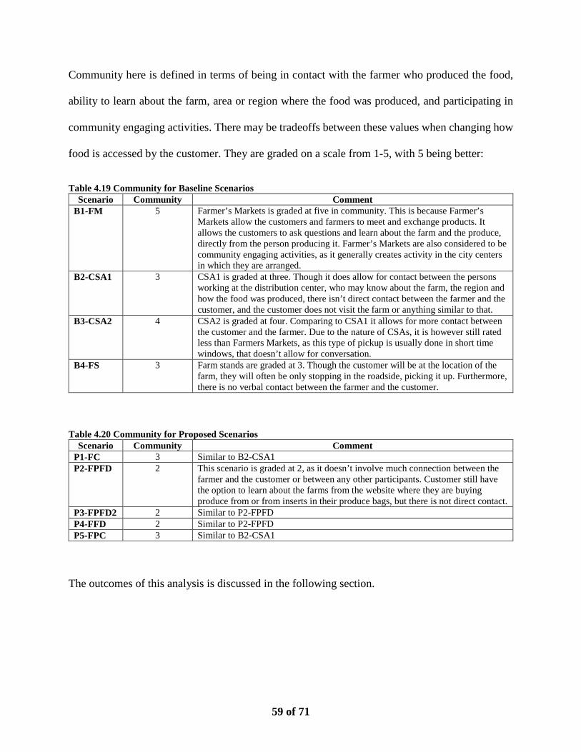
59 of 71

Community here is defined in terms of being in contact with the farmer who produced the food,

ability to learn about the farm, area or region where the food was produced, and participating in

community engaging activities. There may be tradeoffs between these values when changing how

food is accessed by the customer. They are graded on a scale from 1-5, with 5 being better:

Table 4.19 Community for Baseline Scenarios Scenario Community Comment

B1-FM 5 Farmer’s Markets is graded at five in community. This is because Farmer’s Markets allow the customers and farmers to meet and exchange products. It allows the customers to ask questions and learn about the farm and the produce, directly from the person producing it. Farmer’s Markets are also considered to be community engaging activities, as it generally creates activity in the city centers in which they are arranged.

B2-CSA1 3 CSA1 is graded at three. Though it does allow for contact between the persons working at the distribution center, who may know about the farm, the region and how the food was produced, there isn’t direct contact between the farmer and the customer, and the customer does not visit the farm or anything similar to that.

B3-CSA2 4 CSA2 is graded at four. Comparing to CSA1 it allows for more contact between the customer and the farmer. Due to the nature of CSAs, it is however still rated less than Farmers Markets, as this type of pickup is usually done in short time windows, that doesn’t allow for conversation.

B4-FS 3 Farm stands are graded at 3. Though the customer will be at the location of the farm, they will often be only stopping in the roadside, picking it up. Furthermore, there is no verbal contact between the farmer and the customer.

Table 4.20 Community for Proposed Scenarios Scenario Community Comment

P1-FC 3 Similar to B2-CSA1 P2-FPFD 2 This scenario is graded at 2, as it doesn’t involve much connection between the

farmer and the customer or between any other participants. Customer still have the option to learn about the farms from the website where they are buying produce from or from inserts in their produce bags, but there is not direct contact.

P3-FPFD2 2 Similar to P2-FPFD P4-FFD 2 Similar to P2-FPFD P5-FPC 3 Similar to B2-CSA1

The outcomes of this analysis is discussed in the following section.

60 of 71

61 of 71

5. CONCLUSION

This research presented an analysis of a local food distribution system in the state of Washington,

based on a case study of Vashon Island in the Puget Sound. The Vashon Fresh delivery program

requested an analysis of how to optimize a delivery system, and the research was based on this

idea of evaluating different formats for getting local produce to customers. The overall Statement

of Problem was as follows, and will be answered in the following section:

How can local food transportation systems be

structured to allow for local food access without

incurring negative transportation impacts?

Based on this question an analysis was conducted based primarily existing geospatial data,

combined with a survey conducted of inhabitants of the Vashon-Maury Island. The primary goal

was to access a variety of different system designs for bringing local food from farmers to

customers. As the focus on local food and the transportation impact increases, especially in already

dense, polluted urban areas, it is incredibly relevant to attempt to find way to get healthy foods to

as many people as possible, without further negatively impacting the local and global environment

and urban experience. Farmers Markets and Community Supported Agriculture has become

increasingly popular, and is attributed as positively impacting the region in which they are present.

The research presented does not conclude that farmers markets in themselves are negative

alternatives to shopping in grocery stores, as there are benefits to supporting local farmers.

However, the research, does conclude that there are opportunities for developing and improving

the system in which this local food is accessed, to further improve the positive benefits of selecting

and supporting local agriculture. As demonstrated in the research, there are opportunities for

62 of 71

improving the accessibility by offering delivery to customers or more central pick-up points, two

solutions that also have environmental benefits; there are however some tradeoffs for this; when

local food is delivered to the customer as opposed to picked up at e.g. a farmers market, the

personal connection between customer and farm is diminished. It is important to be aware of this

tradeoff, as for many customers, the personal contact, learning about the farm and attending a

market as a recreational activity is an important aspect of selecting this type of produce. However,

when it is possible to substitute some products in a household with local purchases that support

small scale business, the economy of the region, without negatively impacting the transportation

system, this can lead to an overall improvement in how we access food, how food is produced and

sold, and the impacts that it has on the transportation system. In addition to this overall statement

of problem, three sub questions were identified in order to help answer the main question. These

are presented in the following section:

1) What is research currently discussing regarding the state of local food distribution

systems in the U.S.?

Research finds that food supply chains are different from other types of supply chains, as an

increased number of constraints are put on them. These include shorter time limits, requirements

for tracking, specialty packaging, storage, fragility and weight-to-value ratios. Regulation such as

the FDA FSMA further increases costs, as requirements for quality and tracking increases to

protect consumers. For this reason, it is relevant to study food supply chains separately from other

supply chains. Local food has been increasing in popularity, as it is perceived as a healthier food

with a lower environmental impact, along with other intrinsic and extrinsic perceptions of food.

Seen from a systems perspective, local food itself decreases the distance of transportation needed

for getting the produce to the consumer, and it furthermore keeps value in the community in which

63 of 71

it is produced and purchased. There is not a consensus on which geographic limits constitutes

“local”, but producers in Washington agrees that within the county or adjacent county, or closer,

can be considered local. Local food is not perceived as being costlier than other food, as opposed

to organic food is. Local food production and consumption supports local, small scale business

and increases profitability and multi-generational opportunities. Farmers markets have been

gaining popularity, especially in the past 20 years. They provide opportunity for local food access,

and conversation between producer and consumer. However, they are known to have negative

environmental impacts, and be primarily complimentary in terms of a household’s shopping

patterns. Research has been conducted on transporting food, but the fact is that we don’t know

much about how far our food travels. A popular notion is food miles, but looking into the research

behind it, we realize that it is difficult to quantitatively assess the transportation of food in a way

where it is comparable to other systems in another location. Selecting consolidated pick-up

methods or delivery of products, can increase the opportunities for access for customers, and allow

farmers to obtain higher profits; the region to improve its economy and the consumers to access

the food that is appropriate for their values.

2) What are the reasonable assumptions and appropriate evaluation criteria for

modeling and assessing food distribution systems using GIS?

Geographic Information Systems is a widely utilized tool for many different types of transportation

modeling. Using Network Analyst allows the research to make accurate models of smaller or larger

scale, in order to quantitatively assess impacts of spatial movement. However, as with all

modeling, certain decisions and assumptions have to be made regarding how to design the model

that will be used. When modeling, the goal is to get as close as possible to an accurate

representation of reality or what reality could be, with incomplete data. The assumptions made

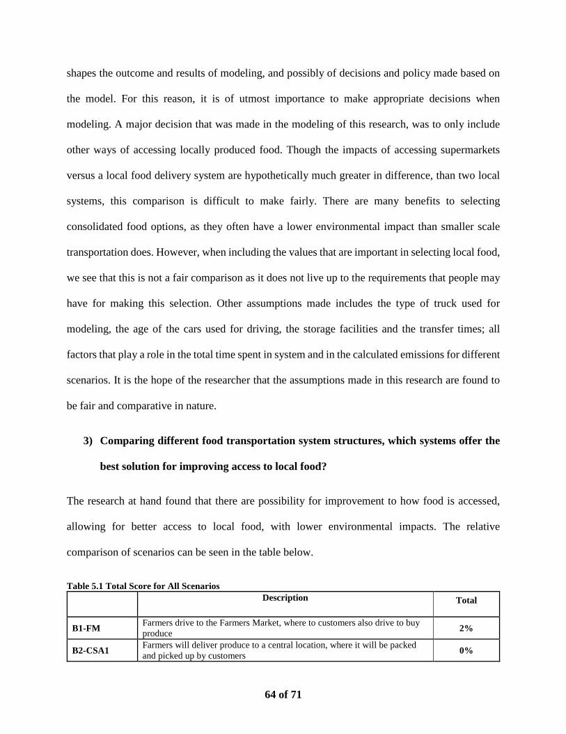
64 of 71

shapes the outcome and results of modeling, and possibly of decisions and policy made based on

the model. For this reason, it is of utmost importance to make appropriate decisions when

modeling. A major decision that was made in the modeling of this research, was to only include

other ways of accessing locally produced food. Though the impacts of accessing supermarkets

versus a local food delivery system are hypothetically much greater in difference, than two local

systems, this comparison is difficult to make fairly. There are many benefits to selecting

consolidated food options, as they often have a lower environmental impact than smaller scale

transportation does. However, when including the values that are important in selecting local food,

we see that this is not a fair comparison as it does not live up to the requirements that people may

have for making this selection. Other assumptions made includes the type of truck used for

modeling, the age of the cars used for driving, the storage facilities and the transfer times; all

factors that play a role in the total time spent in system and in the calculated emissions for different

scenarios. It is the hope of the researcher that the assumptions made in this research are found to

be fair and comparative in nature.

3) Comparing different food transportation system structures, which systems offer the

best solution for improving access to local food?

The research at hand found that there are possibility for improvement to how food is accessed,

allowing for better access to local food, with lower environmental impacts. The relative

comparison of scenarios can be seen in the table below.

Table 5.1 Total Score for All Scenarios Description Total

B1-FM Farmers drive to the Farmers Market, where to customers also drive to buy produce 2%

B2-CSA1 Farmers will deliver produce to a central location, where it will be packed and picked up by customers 0%

65 of 71

B3-CSA2 Customers drive to individual farms. Produce stays on farm. 48%

B4-FS Like CSA2, this solution has customers drive to individual farms to purchase produce 42%

P1-FC Farmers deliver to a central point and customers pick up at this point 3%

P2-FPFD Pickup and delivery is completed during the same trip 83%

P3-FPFD2 Pickup and delivery are completed in two different trips 74%

P4-FFD Farmers deliver to a central point and VF delivers to customers 45%

P5-FPC VF picks up from the farmers and collects at the central point, at where customers will pick up the items from. 33%

P1-FC, B1-FM, and B2-CSA1 are very similar in the setup and in the final scores that they receive,

which are primarily based on the fact that it has all individuals drive to a given point and

differences may not be captured by this modeling. However, when considering accessibility and

community we see that they end up with a grade of 7 (P1-FC), 9 (B1-FM) and 6 (B2-CSA1). This

tells us, that the gain of switching from farmers markets to CSAs or central pickup points are

simply not convincing enough to outweigh the loss of access and the community factor. It is likely

that the P1-FC really is a better solution than the Farmers market, considering that the storage may

be better, it allows more accessibility due to its differing opening hours, and it allows for more

functionality than a farmers market does. This tells us, that there is a need to consider the changes

in storage, transportation and how we use distribution centers, to make the changes to the overall

system, including the decrease in the community factor worthwhile. Noting that many of the most

popular farmers markets are in areas where its visitors won’t have to drive to access them, further

increases the argument for more drastic changes to the transportation system to harness the

environmental benefits of consolidation and substitution. As can be seen in the figure below, four

other scenarios are somewhat similar: B3-CSA2, B4-FS, P4-FFD and P5-FPC. The first two

scenarios are very positive in terms of the total VMT that are connected to them. However, their

access is very low, as it requires customers to drive to specific farms to access the produce. For

some people this may be a solution, but for most, especially in dense urban areas, this is simply

66 of 71

not a feasible way to access food. The two other scenarios has improved access compared to the

two earlier ones, but a lower community rating. There are however benefits in terms of VMT and

time spent in system, when consolidating and using a central location for the distribution of food.

Figure 5.1 Total Score for All Scenarios

The two preferred scenarios are P2-FPFD and P3-FPFD, in which an organization is responsible

for picking up produce from farmers and delivering it in one or two trips. This consolidation greatly

mitigates the environmental impact of small scale food transportation and the issue of lack of

access to local food. The tradeoff of doing so is as described the impact on the community aspect

of accessing local food.

5.1 Questions for Further Research

Through conducting research on a given topic, questions that could benefit from being explored

further occur relatively regularly. This section presents a series of questions that would be

interesting to further examine, to strengthen research within the area:

Total Score for All Scenarios

B1-FM B2-CSA1 B3-CSA2 B4-FS P1-FC P2-FPFD P3-FPFD2 P4-FFD P5-FPC

67 of 71

• The evaluation criteria “Accessibility” is only examined qualitatively in this research. As

the discussion of food deserts and access continues to become more prevalent, it would be

interesting to examine and model the accessibility to farmers markets and other local food.

This could potentially be done through service area analysis in GIS, as has been seen with

food desert analysis based on all types of food outlets.

• Continuing to examine the environmental and transportation impacts of local food systems

could be done by conducting a comparative life cycle analysis of different products, to get

an understanding of the full implications of selecting local food over non-local food.

68 of 71

69 of 71

6. REFERENCES ACS, 2017. Farm Diversification, s.l.: ACS.

Cairns, S., 2004. Delivering Supermarket Shopping: More or Less Traffic?. London: Transport Reviews.

Coley, D., Howard, M. & Winter, M., 2008. Local food, food miles and carbon emissions: A comparison of farm shop and mass distribution approaches. Exeter: Food Policy.

EPA, 2005. Average Annual Emissions and Fuel Consumption for Gasoline-Fueled Passenger Cars and Light Trucks, s.l.: U. S. Environmental Protection Agency.

EPA, 2016. Greenhouse Gas Emissions from a Typical Passenger Vehicle, s.l.: U. S. Environmental Protection Agency.

Esri, 2017. Algorithms used by the ArcGIS Network Analyst extension, s.l.: s.n.

FDA, 2016. FSMA Final Rule on Sanitary Transportation of Human and Animal Food, s.l.: s.n.

Feldmann, C. & Hamm, U., 2014. Consumers’ perceptions and preferences for local food: A review. Witzenhausen: Food Quality and Preference.

Ferrell, C. E., 2004. Home-Based Teleshoppers and Shopping Travel: Do Teleshoppers Travel Less?. DC: Transportation Research Record: Journal of the Transportation Research Board, No. 1894.

FHWA, 2017. Planning Glossary, s.l.: U.S. Department of Transportation.

Gasteyer, S., Hultine, S. A., Cooperband, L. R. & Curry, M. P., 2008. PRODUCE SECTIONS, TOWN SQUARES, AND FARM STANDS: COMPARING LOCAL FOOD SYSTEMS IN COMMUNITY CONTEXT, s.l.: Southern Rural Sociology.

Gracia, A. & Albisu, L.-M., 2001. Food consumption in the European Union: main determinants and country differences. s.l.:Agribusiness 17.

Grunert, K., 1997. What’s in a steak? A cross-cultural study on the quality perception of beef. s.l.:Food Quality and Preference 8.

IHS, 2014. Average Age of Vehicles on the Road Remains Steady at 11.4 years, According to IHS Automotive, s.l.: Business Wire.

KCGIS, 2010. Census Boundaries and Business Tables. s.l.:s.n.

Khan, M., 1981. Evaluation of food selection patterns and. s.l.:CRC Critical Reviews in Food Science and Nutrition.

70 of 71

Lanzendorf, M., 2004. Mobility and accessibility effects of b2c E-commerce: A literature survey. Frankfurt am Main: Tijdschrift voor Economische en Sociale Geografie.

Mannion, M. C. C. G. M., 2000. Factors associated with perceived quality influencing beef consumption behaviour in Ireland. s.l.:British Food Journal.

McKinnon, A., 2003. he Effects of Transport Investment on Logistical Efficiency, s.l.: Logistics Research Centre, Heriot-Watt University.

Mokhtarian, P. L., 2004. A conceptual analysis of the transportation impacts of B2C e-commerce. Davis: Transportation 31.

Morganosky, M. A. & Cude, B. J., 2000. Consumer response to online grocery shopping. Athens: International Journal of Retail & Distribution Management.

Mount, P., 2011. Growing local food: scale and local food systems governance. Guelph: Agricultural Human Values.

Mundler, P. & Rumpus, L., 2012. The energy efficiency of local food systems: A comparison between different modes of distribution. Lyon: Food Policy.

Oberholtzer, L. & Grow, S., 2003. Producer-Only Farmers' Markets in the Mid-Atlantic Region: A Survey of Market Managers, s.l.: Henry A. Wallace Center for Agricultural and Environmental Policy at Winrock International.

Payne, T., 2002. U.S. Farmers' Markets 2000: A Study of Emerging Trends, s.l.: Journal of Food Distribution Research.

Pole, A. & Gray, M., 2012. Farming alone? What’s up with the ‘‘C’’ in community supported agriculture. Montclair, NJ: Agriculatural Human Values.

Ryan, M., 2004. Software Workshop Java: Dijkstra's algorithm, s.l.: THE UNIVERSITY OF BIRMINGHAM School of Computer Science.

Schnell, S. M., 2013. Food miles, local eating, and community supported agriculture: putting local food in its place. Kutztown, PA: Agricultural Human Values.

Selfa, T. & Qazi, J., 2004. Place, taste, or face-to-face? Understanding producer–consumer networks in ‘‘local’’ food systems in Washington State. s.l.:Agriculture and Human Values.

Shepherd, R., 1989. Factors influencing food preference. In: Shepherd, R. (Ed.), Handbook of the Psychophysiology of Human Eating. s.l.:Wiley.

USDA, 2012. Farmers markets and local food marketing: Farmers market growth 1994-2011, s.l.: United States Department of Agriculture.

71 of 71

USDOT, 2014. Table 4-23: Average Fuel Efficiency of U.S. Light Duty Vehicles, s.l.: United States Department of Transportation.

Wakeland, W., Cholette, S. & Venkat, K., 2012. Food transportation issues and reducing carbon footprint, s.l.: Green Technologies in Food Production and Processing.