financialassetreturns,direction-of-change …fdiebold/papers/paper47/1526-5501-2006-52-08... ·...

MANAGEMENT SCIENCEVol. 52, No. 8, August 2006, pp. 1273–1287issn 0025-1909 �eissn 1526-5501 �06 �5208 �1273

informs ®

doi 10.1287/mnsc.1060.0520©2006 INFORMS

Financial Asset Returns, Direction-of-ChangeForecasting, and Volatility Dynamics

Peter F. ChristoffersenFaculty of Management, McGill University, 1001 Sherbrooke Street West, Montreal, Quebec, Canada H3A 1G5 and

Centre for Interuniversity Research and Analysis on Organizations (CIRANO), Montreal, Quebec, Canada, [email protected]

Francis X. DieboldDepartment of Economics, University of Pennsylvania, 3718 Locust Walk, Philadelphia, Pennsylvania 19104-6297 and

National Bureau of Economic Research, Cambridge, Massachusetts, [email protected]

We consider three sets of phenomena that feature prominently in the financial economics literature: (1) con-ditional mean dependence (or lack thereof) in asset returns, (2) dependence (and hence forecastability) in

asset return signs, and (3) dependence (and hence forecastability) in asset return volatilities. We show that theyare very much interrelated and explore the relationships in detail. Among other things, we show that (1) volatil-ity dependence produces sign dependence, so long as expected returns are nonzero, so that one should expectsign dependence, given the overwhelming evidence of volatility dependence; (2) it is statistically possible tohave sign dependence without conditional mean dependence; (3) sign dependence is not likely to be found viaanalysis of sign autocorrelations, runs tests, or traditional market timing tests because of the special nonlinearnature of sign dependence, so that traditional market timing tests are best viewed as tests for sign dependencearising from variation in expected returns rather than from variation in volatility or higher moments; (4) signdependence is not likely to be found in very high-frequency (e.g., daily) or very low-frequency (e.g., annual)returns; instead, it is more likely to be found at intermediate return horizons; and (5) the link between volatilitydependence and sign dependence remains intact in conditionally non-Gaussian environments, for example, withtime-varying conditional skewness and/or kurtosis.

Key words : return sign dependence, market timing; predictionHistory : Accepted by David Hsieh, finance; received February 25, 2004. This paper was with the authors9 months for 3 revisions.

1. IntroductionWe consider three sets of phenomena that featureprominently in the financial economics literature:(1) approximate conditional mean independence (andhence little or no forecastability) in asset returns,(2) dependence (and hence forecastability) in assetreturn signs, and (3) dependence (and hence fore-castability) in asset return volatilities. We argue thatthey are very much interrelated, forming a tangledand intriguing web, a full understanding of whichleads to a deeper understanding of the subtleties offinancial market dynamics. Let us introduce themin turn.First, consider conditional mean independence,

by which we mean that an asset return’s condi-tional mean does not vary with the conditioninginformation set. Approximate conditional mean inde-pendence then implies that out-of-sample return fore-casting will be difficult, if not impossible. This viewis widely held and stems from both introspection andobservation. That is, financial economic theory sug-gests that asset returns should not be easily forecastusing readily available information and forecasting

techniques, and a broad interpretation of four decadesof empirical work suggests that the data supportthe theory (e.g., Fama 1970, 1991). Consequently, webelieve that conditional mean independence is rea-sonably viewed as a good working approximation toasset return dynamics.1

Second, consider dependence and hence forecasta-bility of market direction (the return sign). Profitabletrading strategies result from successful forecastingof market direction, quite apart from whether one issuccessful at forecasting returns themselves. A well-known and classic example, discussed routinely even

1 We emphasize the word “approximation” because weak condi-tional mean dependence may appear at both long horizons (e.g.,Fama and French 1988, 1989; Campbell and Shiller 1988) andshort horizons (e.g., Lo and MacKinlay 1999) for a variety of rea-sons, ranging from low-frequency variation in risk premia to high-frequency variation in market microstructure noise. The evidenceof long-horizon conditional mean dependence remains controver-sial, however, because of serious statistical complications includ-ing possibly spurious regressions (e.g., Kirby 1997), data snoopingbiases (e.g., Foster et al. 1997), and small sample biases (Nelson andKim 1993), which may distort standard inference procedures whenapplied to long-horizon prediction regressions.

1273

Christoffersen, P.F. and Diebold, F.X. (2006),"Financial Asset Returns, Direction-of-Change Forecasting, and Volatility Dynamics,"

Management Science, 52, 1273-1287

Christoffersen and Diebold: Financial Asset Returns1274 Management Science 52(8), pp. 1273–1287, © 2006 INFORMS

at the MBA textbook level (e.g., Levich 2001, Chap-ter 8), involves trading in speculative markets. If, forexample, the yen-dollar exchange rate is expected toincrease, reflecting expected depreciation of the yenrelative to the dollar, and hence a negative expectedreturn on the yen, one would sell yen for dollar,whether in the spot or derivatives markets. Positiveprofits will be made when the sign forecast is cor-rect. Generalizations to multiple asset classes, suchas stock and bond markets, involve basing alloca-tion strategies on forecasts of the sign of the returnspread. Recent literature shows that asset return signforecasting can often be done with surprising suc-cess; see, among others, Breen et al. (1989), Leitchand Tanner (1991), Wagner et al. (1992), Pesaran andTimmermann (1995), Kuan and Liu (1995), Larsenand Wozniak (1995), Womack (1996), Gencay (1998),Leung et al. (2000), Elliott and Ito (1999), White (2000),Pesaran and Timmermann (2004), and Cheung et al.(2005).Finally, consider dependence and forecastability of

asset return volatility. A huge literature documentsthe notable dependence, and hence forecastability, ofasset return volatility, with important implications notonly for asset allocation, but also for asset pricingand risk management. Bollerslev et al. (1992) pro-vide a fine review of evidence in the GARCH tradi-tion, while Ghysels et al. (1996) survey results fromstochastic volatility modeling, Franses and van Dijk(2000) survey results from regime-switching volatil-ity models, and Andersen et al. (2005a) survey resultsfrom realized volatility modeling. Interesting exten-sions include models of time variation in higher-ordered conditional moments, such as the conditionalskewness models of Harvey and Siddique (2000) andthe conditional density model of Hansen (1994). Therecent literature also contains intriguing theoreticalwork explaining the empirical phenomenon of volatil-ity forecastability, such as Brock and Hommes (1997)and de Fontnouvelle (2000).In this paper, we characterize in detail the rela-

tionships among the three phenomena and threeliteratures discussed briefly above: (1) asset returnconditional mean independence, (2) sign dependence,and (3) conditional variance dependence. It is wellknown that conditional mean independence and con-ditional variance dependence are statistically compat-ible. However, much less is known in general aboutsign dependence, and in particular about the relation-ship of sign dependence to conditional mean inde-pendence and volatility dependence. Hence, we focusthroughout on sign dependence. Among other things,we show that(1) Volatility dependence produces sign depen-

dence, so long as expected returns are nonzero.Hence, one should expect sign dependence, given theoverwhelming evidence of volatility dependence.

(2) It is statistically possible to have sign (andvolatility) dependence, while at the same time, meanindependence.(3) Sign dependence is not likely to be found via

analysis of sign autocorrelations or other tests (suchas runs tests or traditional tests of market timing)because the nature of sign dependence is highlynonlinear.(4) Sign dependence is not likely to be found in

high-frequency (e.g., daily) or low-frequency (e.g.,annual) returns. Instead, it is more likely to appear atintermediate return horizons of two or three months.(5) The link between volatility forecastability and

sign forecastability remains intact in conditionallynon-Gaussian environments, for example, with time-varying conditional skewness and/or kurtosis; in fact,it is significantly enriched.We derive results (1), (2), and (5) theoretically in

a general setting, we derive (3) and (4) via a com-plementary calibrated simulation experiment using apopular model of return dynamics, and we provide apreliminary empirical exploration using the S&P 500in conjunction with RiskMetrics volatility forecasts.Before moving on, we wish to emphasize that our

basic contention, namely, that sign dependence existsand has fundamental connections to volatility depen-dence, in no way requires conditional mean indepen-dence; instead, we simply invoke conditional meanindependence to make our point as clearly as pos-sible. This is fortunate because although conditionalmean independence is a reasonable approximation formany purposes, it is also the subject of some con-troversy on both the theoretical and empirical fronts,with both theory and empirics ultimately provinginconclusive. Classical dynamic asset pricing theorypredicts a positive equilibrium relationship betweenconditional first and second moments (e.g., Merton1973, Ferson and Harvey 1991), but it is now rec-ognized that theory is also consistent with a nega-tive relationship (e.g., Abel 1988, Backus and Gregory1993, Gennotte and Marsh 1993). Similarly inconclu-sive results hold on the empirical side: positive butoften insignificant dependence is found in Baillie andDeGennaro (1990), French et al. (1987), Campbell andHentschel (1992), and Ghysels et al. (2005), whereasnegative dependence is found in Campbell (1987),Nelson (1991), Lettau and Ludvigson (2005), andBrandt and Kang (2004), and both are found in Glostenet al. (1993), Harvey (2001), and Turner et al. (1989).We proceed as follows. In §2, we build intuition

by sketching the main results in simple contexts,focusing primarily on the conditionally Gaussian case.We discuss the basic framework, we arrive at the basicresult that volatility dynamics produce sign dynam-ics, and we draw the implications. In §§3 and 4, wefocus in greater depth on sign dependence, and we

Christoffersen and Diebold: Financial Asset ReturnsManagement Science 52(8), pp. 1273–1287, © 2006 INFORMS 1275

provide basic results on sign realizations, sign fore-casts, and the relation between the two, stressingboth the measurement (§3) and detection (§4) of signforecastability. In §5, we perform a detailed simula-tion experiment, which not only illustrates our basicresults but also extends them significantly, by charac-terizing the nature of sign forecastability as a functionof forecast horizon. We provide an illustrative empir-ical application in §6, and conclude in §7.

2. Conditional Mean Dependence,Sign Dependence, and VolatilityDependence: Basic Results

Here, we explore the links between conditional meandependence, sign dependence, and volatility depen-dence. We have used the terms repeatedly, but thusfar, not defined them precisely, relying instead onreaders’ intuition, so let us begin with some pre-cise definitions. First, we will say that a return seriesRt+1 displays conditional mean dependence (condi-tional mean dynamics, conditional mean forecasta-bility, conditional mean predictability) if E�Rt+1 ��t�varies with �t .2 Second, we will say that Rt+1 dis-plays sign dependence (sign dynamics, sign forecasta-bility, sign predictability) if the return sign indicatorseries I�Rt+1 > 0� displays conditional mean depen-dence; that is, if E�I�Rt+1 > 0� � �t� varies with �t .3

Finally, we will say that Rt+1 displays conditionalvariance dependence (conditional variance dynam-ics, conditional variance forecastability, conditionalvariance predictability, volatility dependence, volatil-ity dynamics, volatility forecastability, volatility pre-dictability) if 2

t+1 � t ≡Var�Rt+1 ��t� varies with �t .We now proceed to characterize the relationships

among sign, volatility dynamics, and conditionalmean dynamics.

2.1. Sign Dynamics Follow from VolatilityDynamics

Consider the prevalence of volatility dynamics inhigh-frequency asset returns, and the positive ex-pected returns earned on risky assets. To take the sim-plest possible example, which nevertheless conveysall of the basic points, assume that the returns on ageneric risky asset are distributed as

Rt+1 ��t ∼N��2t+1 � t�� > 0� (1)

2 Here and throughout, “returns” are excess returns relative to therisk-free rate.3 Equivalently, Rt+1 displays sign dependence if the conditionalprobability of a positive return, Pr�Rt+1 > 0 � �t�, varies with �t

because Pr�Rt+1 > 0 ��t�= E�I�Rt+1� > 0 ��t�.

and therefore display conditional variance depen-dence but no conditional mean dependence. Theprobability of a positive return is then

Prt�Rt+1 > 0� = 1−Prt�Rt+1 < 0�

= 1−Pr(Rt+1−�

t+1 � t<

−�

t+1 � t

)

= �

(�

t+1 � t

)� (2)

where ��·� is the N�0�1� cumulative density function(c.d.f.). Note that although the distribution is symmet-ric around the conditional mean, and the conditionalmean is constant by assumption, the sign of the returnis nevertheless forecastable because the probability ofa positive return is time varying (and above 0.5 if �>0). As volatility moves, so too does the probability ofa positive return: the higher the volatility, the lowerthe probability of a positive return, as illustrated inFigure 1.The surprising result that the sign of the return

is forecastable although the conditional mean is con-stant hinges interestingly on the interaction of anonzero mean return and nonconstant volatility. Azero mean would render the sign unforecastable, aswould constant volatility; hence the tradition in finan-cial econometrics of removing unconditional meansand working with zero-mean series disguises signforecastability. Note also that a large volatility relativeto the mean renders the sign nearly unpredictable.It is interesting to note that the key link betweensign forecastability and volatility dynamics parallelsthe literature on optimal prediction under asymmet-ric loss. In sign forecasting, volatility dynamics inter-act with a nonzero mean to produce time variationin the probability of a positive return, and hence signforecastability. In forecasting under asymmetric loss,as in Christoffersen and Diebold (1996, 1997), volatil-ity dynamics similarly produce time variation in theoptimal point forecast of a series with a constant con-ditional mean.Our setup above was intentionally simple, but it

is easy to see that the results are maintained undera number of interesting variations. To take just oneexample (we discuss several in the online supplementon the Management Science website at http://mansci.pubs.informs.org/ecompanion.html), note that ifreturns are conditionally non-Gaussian (e.g., con-ditionally skewed), the result in Equation (2) thatvolatility forecastability implies sign forecastabilitystill holds.

2.2. Sign Dynamics Do Not Require ConditionalMean Dynamics

Forecasting market direction is of interest for activeasset allocation, and a substantial body of evidence


Figure 1 The Dependence of Sign Probability on Volatility

0

1

2

3

4

5

6

7

8

9

–0.3 –0.2 –0.1 0.0 0.1 0.2 0.3 0.4 0.5

Den

sity

Return

σ = 0.05

σ = 0.15

Notes. We show two Gaussian return densities, each with expected return of 10%. The first return has a standard deviation of 5%, and hence is positivewith probability 0.98 (the area to the right of zero under the more-peaked density function). The second return has a standard deviation of 15%, and hence ispositive with smaller probability 0.75 (the area to the right of zero under the less-peaked density function).

suggests that it can be done, as per the references givenearlier. Successful directional forecasting implies thatreturns must be somehow dependent. When direc-tional forecasting is found to be empirically success-ful, it is tempting to assert that it is driven by (per-haps subtle) nonlinear conditional mean dependence,which would be missed in standard analyses of (lin-ear) dependence, such as those based on return auto-correlations.The key insight is that although sign dynamics

could be due to conditional mean dependence, theyneed not be. In particular, we have demonstratedthat volatility dynamics produce sign dynamics,so that one should expect sign dynamics in assetreturns, given the overwhelming evidence of volatil-ity dynamics, even if returns display near conditionalmean independence.Moreover, as noted above, in a general equilibrium

involving risk-averse market participants observedprices will, of course, not in general evolve as mar-tingales, which is to say that observed returns mayin general display some conditional mean dynamicsbecause of perhaps time-varying risk premia over thebusiness cycle. Any such conditional mean dynam-ics may, of course, contribute to sign forecastabil-ity as well. In our analysis, we intentionally assumethe absence of conditional mean dynamics for sev-eral reasons. First, as discussed earlier, the evidencesuggests that conditional mean independence is areasonable empirical approximation to asset returndynamics, despite the fact that dynamic asset pric-ing theory predicts dependence between first andsecond moments. Second, we want to focus on thesubtle and little-understood connection between signdynamics and volatility dynamics. Third, standardexpansions suggest that even if conditional mean

dynamics are operative, one may expect that con-ditional variance dynamics will dominate.4 To seethis, consider a Taylor series expansion of �t+1 � t/t+1 � tabout the mean

�t+1 � t/t+1 � t ≈ �/ + ��t+1 � t −��−1

+ �−1t+1 � t −−1�� (3)

Based on this, consider the variance of �t+1 � t/t+1 � t . Tofirst order, the variance of �t+1 � t is multiplied by −2,which is a large number, while the variance of 1/t+1 � tis multiplied by �2, a smaller number. However, thevariance of 1/t+1 � t is huge and should be the domi-nant term.

2.3. An Intriguing DecompositionIt is interesting to interpret the phenomena at handthrough the decomposition5

Rt+1 = sign�Rt+1� · �Rt+1�� (4)

In the simple models just described (and, to a goodapproximation, in observed return data), both ofthe right-hand side components of returns displaypersistent dynamics and hence are forecastable, yetthe left-hand side variable, returns themselves, areunforecastable. This is an example of a nonlinear“common feature,” in the terminology of Engle andKozicki (1993): both signs of returns and absolutereturns are conditional mean dependent and henceforecastable, yet their product can be conditionalmean independent, and hence unforecastable.

4 The authors thank a referee for suggesting this, and for the Taylorseries argument.5 See Rydberg and Shephard (2003) for an extensive and authorita-tive treatment of this and related decompositions in the context ofultrahigh-frequency financial asset price movements.


3. Measuring the Strength of SignForecastability

Here, we examine a number of questions relevant tomeasuring sign forecastability. How, if at all, does thederivative of a sign forecast with respect to volatilityvary as a function of volatility, and in what volatilityregion is the derivative largest? What is the correla-tion between sign forecasts and realizations, and how,if at all, is the correlation related to the volatility ofsign forecasts?

3.1. The Responsiveness of Sign Forecasts toVolatility Changes

In the simple setup developed thus far, we achieveprobability forecastability only from volatility dynam-ics. A key issue is how much the probability forecastchanges when the volatility changes, and the obviousmeasure is the derivative

�= �Prt�Rt+1 > 0��t+1 � t

� (5)

where we choose the notation � for “responsive-ness.”6 Immediately,

�=−f

( −�

t+1 � t

)(�

2t+1 � t

)� (6)

where f �·� is the probability density function (p.d.f.)of standardized returns.In Figure 2, we work in a Gaussian environment

and plot � as a function of the information ratio, �/ .Note that � is always negative (i.e., the probabilityof a positive return is always decreasing in the con-ditional standard deviation). Crucially, however, � isnot monotone in �/ ; instead, it achieves a minimumat �/ =√

2= 1�41. This makes sense: for �/ closeto zero, the conditional probability of a positive returncan deviate little from 1/2, and hence responsivenessis tiny. Similarly, for very large �/ , the conditionalprobability of a positive return can deviate little from1, and hence responsiveness is again tiny. Interme-diate values of �/ , however, can produce greaterresponsiveness. The maximal forecastability as mea-sured by � that occurs when �/ ≈ 1�41 is rather highfor an information ratio. The frequency with whichwe hit that “sweet spot” depends on the volatility ofvolatility, to which we shall return.

3.2. The Correlation between Sign Forecasts andRealizations

To characterize the correlation between sign forecastsand realizations, first note that

Cov�It+1�Pt+1 � t� = E�It+1Pt+1 � t�−E�It+1�E�Pt+1 � t�

= E�It+1Pt+1 � t�− P 2� (7)

6 This is also known as the “marginal effect” in the binary responseliterature.

Figure 2 Responsiveness of Sign Probability to Volatility MovementsPlotted Against the Information Ratio, �/�

–3.0

–2.5

–2.0

–1.5

–1.0

–0.5

0.0

0 1 2 3 4 5

Der

ivat

ive

µ/σ

Notes. We plot �t , the derivative of the probability of a positive return withrespect to return volatility, as a function of the information ratio, �/� . Weassume Gaussian returns.

where P is the unconditional probability of a positivereturn and It+1 is the indicator variable of an ex postrealized positive return. Second, use the law of iter-ated expectations to get

E�It+1Pt+1 � t� = E�Et�It+1Pt+1 � t��= E�Et�It+1�Pt+1 � t�

= E�P 2t+1 � t�� (8)

Hence, we have

Cov�It+1�Pt+1 � t�= E�P 2t+1 � t�− P 2 =Var�Pt+1 � t�� (9)

so the covariance between the forecast and the real-ization is equal to the variance of the forecast.7 Con-verting to correlation, we can write

Corr�It+1�Pt+1 � t� =Var�Pt+1 � t�

Std�It+1�Std�Pt+1 � t�

= Std�Pt+1 � t�√P�1− P�

� (10)

where P = E�It�. Note that the correlation betweensign forecasts and realizations depends only on thestandard deviation of the forecast, which, of course,will depend on the particular return process at hand.Despite its generality, the correlation expression fur-nishes considerable insight. In particular, because theoptimal probability forecast Pt+1 � t is driven entirelyby the volatility t+1 � t , we have that Corr�It+1�Pt+1 � t�,which is proportional to Std�Pt+1 � t�, is therefore drivenby the volatility of volatility.

4. Detecting Sign ForecastabilityNow, we examine questions relevant to the detec-tion of sign forecastability. First, we examine theserial correlation structure of sign realizations, and

7 Alternatively, and perhaps more intuitively, note that regressionof It+1 on Pt+1 � t yields a unit coefficient by definition of It+1 andPt+1 � t . That is, Cov�It+1�Pt+1 � t �/Var�Pt+1 � t � = 1, which implies thatCov�It+1�Pt+1 � t �=Var�Pt+1 � t �.


we argue that it is not likely to be useful for iden-tifying sign forecastability because the optimal signpredictor turns out to be highly nonlinear. Hence,linear diagnostic tools discard valuable information.Next, we study the efficacy of runs tests for detectingsign forecastability and show that they have paralleldeficiencies. Finally, we examine the ability of tradi-tional market timing tests to detect sign forecastabil-ity, and we argue that although they may have goodpower to detect sign forecastability arising from time-varying expected returns, they have little or no powerto detect sign forecastability arising from variation involatility (or higher-ordered conditional moments).

4.1. Serial Correlation of SignsThe basic insight is simply that

Corr�It+1� It� <Corr�Pt+1 � t� It+1�� (11)

which follows immediately from the fact that the opti-mal time-t forecast of It+1, Pt+1 � t has a higher corre-lation with It+1 than anything else observed at timet, including It .8 The inequality leads one to suspect—although, of course, it does not definitively prove—that the size of the sign autocorrelation is likely to bemuch less than the maximum attainable because It isnot likely to be highly correlated with Pt+1 � t , which isdriven directly by t+1 � t , not It . Hence, we conjecturethat the autocorrelations of the sign sequence may besmall, even if sign predictability is high. In §5, weshall provide a quantitative assessment of this effectin a realistically calibrated simulation.

4.2. Runs TestsWorking with a 0-1 sign sequence naturally leads oneto consider tests of sign forecastability based on thenumber of runs in the sign sequence, and there is along tradition of doing so in empirical finance; see,for example, Campbell et al. (1997, Chapter 2) for anoverview. We now consider whether runs tests arelikely to be more useful for detecting sign depen-dence than the serial correlation coefficients discussedabove.A run is simply a string of consecutive zeros or

ones. Hence, the number of runs is the number ofswitches from 0 to 1, plus the number of switchesfrom 1 to 0, plus 1,

Nruns = 1+∑t

�1− It�It+1+∑t

It�1− It+1�� (12)

which can be written as

Nruns = 1+ 2 PT − 2∑t

ItIt+1� (13)

8 The inequality can also be established by formally deriving theequality Corr�It+1� It�=Corr�Pt+1 � t� It+1�Corr�Pt+1 � t� It�.

where P = �1/T �∑

t It . Solving the Nruns equation for∑t ItIt+1 and exploiting the fact that I 2t = It yields the

estimator,

Corr�It+1� It� =�1/T �

∑t ItIt+1− P 2

P�1− P�= 1− Nruns− 1

2T P�1− P� � (14)

This expression makes clear that there is no informa-tion in the number of runs in a sign sequence thatis not also in the first-order autocorrelation of thesequence, and conversely. Thus, our earlier conjec-ture that sign predictability is unlikely to be foundusing autocorrelations of the sign sequence translatesas well into a conjecture that it is unlikely to be foundusing runs tests. In general, tests that rely only onthe sign sequence omit important information aboutvolatility dynamics, which is potentially valuable fordetecting sign predictability.

4.3. Market Timing TestsHere, we discuss some popular market timing testsand their relationship to return sign forecasts, and weargue that none of them are likely to be useful for cap-turing sign forecastability when it arises via volatilitydynamics, as we have emphasized.The literature on market timing is intimately con-

cerned with signs and sign forecasting. For example,Henriksson and Merton (1981) argue that p1 + p2 − 1can be interpreted as the multiplier to apply to thevalue of perfect market timing, where p1 is the proba-bility of a correctly forecasted negative return and p2is the probability of a correctly forecasted positivereturn. Breen et al. (1989) show that in the regression

I�Rt+1 > 0�= a+ bI�Pt+1 � t > 0�5�+ et+1� (15)

we have that b = p1 + p2 − 1. Hence, the absence ofHenriksson and Merton (1981) market timing abilitycorresponds to b= 0, which is easily tested using stan-dard methods. Cumby and Modest (1987) examinethe closely related regression,

Rt+1 = a+ bI�Pt+1 � t > 0�5�+ et+1� (16)

and similarly test the significance of b.9

Note that all of the tests above process Pt+1 � t in aparticular way: Pt+1 � t enters them only through theindicator function I�Pt+1 � t > 0�5�.10 Hence, for exam-ple, a Pt+1 � t of 0.5001 is treated fundamentally differ-ently from a Pt+1 � t of 0.4999, whereas a Pt+1 � t of 0.9999

9 See also Merton (1981), Whitelaw (1997), and Busse (1999). Note,however, that this framework does not include the quadratic regres-sion tests of Treynor and Mazuy (1966) and Ferson and Schadt(1996), which are used in mutual fund performance evaluation.10 The same is true for generalizations of the Henriksson andMerton (1981) test, such as Pesaran and Timmermann (1992).


is treated no differently from a Pt+1 � t of 0.5001. Thisis particularly unfortunate because although volatilitydynamics lead to sign forecastability (i.e., variation inPt+1 � t), the time-varying Pt+1 � t may well never dropbelow 0.5. Such is the case, for example, in the leadingexample of a fixed positive expected return with sym-metric conditional density analyzed earlier, so that thetests discussed above would have no power to detectsign dependence. Hence, the traditional market tim-ing tests are best viewed as tests for sign dependencearising from variation in expected returns rather thanfrom variation in volatility (or higher-ordered condi-tional moments).

5. Sign Forecasting for Various DataFrequencies and Forecast Horizons:A Simulation Experiment

We have shown that return sign forecastability arisesfrom the interaction of nonzero expected returns andvolatility forecastability. As expected returns approachzero, or as volatility forecastability approaches zero,sign forecastability approaches zero.11 Hence, onedoes not expect strong sign forecastability for veryhigh-frequency returns such as daily, despite theirhigh volatility forecastability, because expected dailyreturns are negligible. Similarly, one does not expectstrong sign forecastability for very low-frequencyreturns such as annual, despite the high expectedreturns, because annual return volatility forecastabil-ity is negligible. One might therefore conjecture thatsign forecastability will be highest at some interme-diate horizon between such very short and very longextremes. In this section, we evaluate this conjecture.When analyzing sign dynamics at various hori-

zons, one is quickly faced with the challenge thatfew discrete-time dynamic models with time-varyingvolatility are closed in distribution under increasinghorizons.12 We therefore work with Heston’s (1993)affine continuous-time stochastic volatility model,which is arguably the most widely applied modernunivariate stochastic process for equity and equityindex returns. In Heston’s (1993) model, the condi-tional characteristic function is known for any hori-zon, so Fourier inversion techniques can be used tocompute sign probability forecasts.

11 Of course, higher-ordered conditional moment dynamics can alsocontribute to sign predictability, as we discuss in detail in theonline supplement.12 For penetrating insight into the difficulties involved in the tempo-ral aggregation of discrete-time volatility models, see Meddahi andRenault (2004), Meddahi (2001), Darolles et al. (2001), and Hestonand Nandi (2000).

5.1. Simulation DesignThe stochastic volatility model parsimoniously cap-tures many of the stylized facts of asset returns,including skewness, leptokurtosis, and volatility per-sistence, and its conditional density can be calcu-lated easily at any forecast horizon. For all of thesereasons—both substantive and methodological—ithas become a standard benchmark in empirical assetpricing.13

The Heston (1993) stochastic volatility model is

dS�t�=�Sdt+�t�Sdz1�

d2�t�= ��−2�t��dt+��t�dz2�(17)

where S�t� is the asset price process and 2�t� is thevariance process, and where Corr�dz1�dz2� = �. Theexpected instantaneous rate of return is �, the long-run variance is �, the speed of variance adjustmentis governed by �, and the volatility of volatility isgoverned by �.Using Ito’s lemma, the stochastic volatility process

can conveniently be written in terms of the log assetprice, x�t�, as

dx�t�= ��−2�t�/2�dt+�t�dz1�

d2�t�= ��−2�t��dt+��t�dz2�(18)

Note that although the instantaneous drift is sim-ply a constant, the continuously compounded returnhas a slightly time-varying mean from the Itotransformation.The probability of an increase in the asset price

between time t and t + ! , or equivalently, the prob-ability of a positive return during "t� t + !#, can becalculated using the inverse characteristic functiontechnique.14 In particular,

Pt+! � t ≡ Pr�x�t+ !�≥ x�t� � x�t�= x� 2�t�= 2�

= 12+ 1

$

∫ �

0Re

(exp�−i&x�f �x�2� !'&�

i&

)d&�

(19)

where f �x�2� !'&� is the characteristic function forhorizon ! , i=√−1, Re�·� takes the real part of a com-plex number, and the characteristic function is

f �x�2� !'&�= exp�C�!�&�+D�!�&�2+ i&x�� (20)

13 The stochastic volatility model has been estimated by Andersenet al. (2002), Bakshi et al. (1997), Benzoni (2002), Chernov et al.(2003), Chernov and Ghysels (2000), Eraker et al. (2003), Jones(2003), and Pan (2002), among others. We intentionally work witha very simple version of the model, with a single volatility factor,no volatility jumps, and no volatility long memory. One could, ofcourse, examine even richer models with multiple volatility factorsand/or volatility jumps as in Alizadeh et al. (2002), Bates (2000),Chernov et al. (2003), and Duffie et al. (2000), and long memory involatility as in Andersen et al. (2001a, b; 2003).14 As in the Gaussian case, computation of the sign probabilityrequires numerical integration, but the well-behaved integrand ren-ders the integration straightforward.


where

C�!�&�=�&i! + ��

�2

(��−��&i+ d�!

− 2 log(1− g exp�d!�

1− g

))� (21)

D�!�&�=(�−��&i+ d

�2

)(1− exp�d!�1− g exp�d!�

)� (22)

g = �−��&i+ d

�−��&i− d� (23)

and

d=√��&i−��2+�2�&i+&2�� (24)

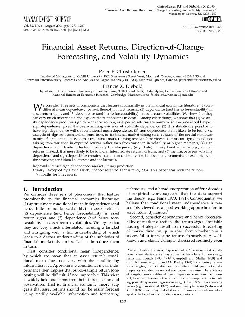
As we have shown, the structure of the Hestonmodel makes certain key calculations tractable, whichexplains its popularity. We will now exploit thattractability to illustrate several important aspects ofoptimal sign forecasting, including the existence of anontrivial optimal horizon for sign prediction. Beforedoing so, however, we note that the Heston modelactually limits the possible amount of sign predictabil-ity. In particular, to ensure in discrete-time simula-tions that the variance process stays strictly positivealmost surely in the Heston model, it is necessary torestrict the volatility of volatility ��, such that �2 ≤2��. This limits the amount of sign predictability thatthe Heston model can generate because it requires thevolatility of volatility to be small relative to the uncon-ditional variance and the conditional variance persis-tence, whereas sign predictability is greatest when thevolatility of volatility is high, when conditional vari-ance persistence is high, and when the unconditionalvariance is low relative to the mean. Other stochasticvolatility specifications, although less tractable mathe-matically, imply no such limits to sign predictability.15

In this sense, then, our simulation results below onsign predictability using the Heston model as a data-generating process are, if anything, conservative rela-tive to those that could be obtained using alternativemodels.We simulate prices at five-minute intervals and

assume 24-hour trading with 250 trading days peryear. For the purpose of sign prediction, we pro-ceed by discarding the intraday observations and takedaily to be the highest frequency of interest. We cal-ibrate the parameters to typical values estimated inthe empirical literature. Our benchmark values are�= 0�10, � = 2, � = 0�015, � = 0�15, and � = −0�50,

15 The volatility of volatility restriction in the Heston (1993) modelhas been found to be restrictive in option valuation as well. Cir-cumventing the restriction, Duffie et al. (2000) suggest a modelwith correlated jumps in returns and jumps in volatility. Bakshi andCao (2003) find that the new model significantly improves on theHeston (1993) model when valuating individual equity options.

which imply a daily mean of about 0.037%, a dailyunconditional standard deviation of 0.77%, uncon-ditional skewness of about −0�1, and unconditionalexcess kurtosis of about 1.16 The annualized meanreversion parameter �= 2 implies a daily persistenceof about 1− 2/250 = 0�99 in a standard GARCH(1,1)model. Note also that the parameters satisfy the �2 ≤2�� condition.

5.2. Simulation ResultsIn Figure 3, we plot the sign forecasts from a typi-cal sample path of the simulated process, computedusing (19). We show daily, weekly, monthly, quarterly,semiannual, and annual conditional as well as uncon-ditional sign probabilities. As we move from daily toannual returns, the volatility of the conditional signprobabilities first increases and then decreases. By(10), this supports our conjecture that sign predictabil-ity should increase and then decrease with horizon.In contrast, the unconditional probability of a positivereturn increases monotonically (and at a decreasingrate) with horizon.In Figure 4, we focus more directly and thoroughly

on our conjecture that sign dynamics will be mostprevalent at intermediate frequencies; examining thecorrelation between sign forecasts and realizationsas a function of horizon. Consider first the top linewhere � = 0�10, which is our benchmark parametervalue. The correlation is quite low for the highest fre-quency returns, then it increases, and then it tapersoff again as we aggregate toward annual returns.The correlation is highest at horizons of approxi-mately 2–3 months (corresponding to 40–60 tradingdays). Interestingly, then, despite the fact that signpredictability is driven by volatility predictability,which is highest at very high frequencies, the interac-tion between decreasing volatility predictability andincreasing expected returns under temporal aggrega-tion results in maximization of sign predictability atmedium horizons.Consider now the middle and lower lines in

Figure 4 corresponding to � = 0�05 and � = 0,respectively, with all other parameters kept at theirbenchmark values. As expected, signs are less fore-castable at all horizons for smaller �; the figureprovides a precise quantitative characterization. Inter-estingly, some sign forecastability remains even when�= 0 because of the nonzero leverage effect, �, inter-acting with the volatility dynamics.17

16 In the online supplement, we explore an alternative parameteri-zation with no leverage, and the results are qualitatively similar.17 It is interesting to note that even when both drift and leverage arezero, there is a small degree of sign forecastability as the horizonincreases, coming from the Ito term, − 2�t�/2, in the drift of thelog price process. Meddahi and Renault (2004) find similar effects


Figure 3 Time Series of Conditional Sign Probabilities—Various Return Horizons

0.5

0.6

0.7

0.8

0.9

50 100 150 200 250 300 350 400 450 500

Pro

babi

lity

0.5

0.6

0.7

0.8

0.9

Pro

babi

lity

0.5

0.6

0.7

0.8

0.9

Pro

babi

lity

0.5

0.6

0.7

0.8

0.9

Pro

babi

lity

0.5

0.6

0.7

0.8

0.9

Pro

babi

lity

0.5

0.6

0.7

0.8

0.9

Pro

babi

lity

Time

50 100 150 200 250 300 350 400 450 500

Time

50 100 150 200 250 300 350 400 450 500

Time

50 100 150 200 250 300 350 400 450 500

Time

50 100 150 200 250 300 350 400 450 500

Time50 100 150 200 250 300 350 400 450 500

Time

Daily returns Weekly returns

Monthly returns Quarterly returns

Semiannual returns Annual returns

Notes. We simulate asset prices from a stochastic volatility model parameterized as dS�t� = 010Sdt + � �t�S dz1 and d� 2�t� = 2�0015 − � 2�t�� dt +015� �t� dz2, with Corr�dz1� dz2�=−05. We then calculate at each of 500 periods the conditional probability of a positive return at daily, weekly, monthly, andannual horizons. The horizontal line in each subplot denotes the unconditional probability of a positive return, which equals the average conditional probability.

In Figure 5, we explore the effects of lower volatil-ity persistence. The top line again corresponds to ourbenchmark parameter value; that is, �= 2. The mid-dle line shows the correlation between sign forecastsand realizations when �= 5 (corresponding to a dailyvolatility persistence of about 0.98) and the bottomline when �= 10 (corresponding to a daily volatility

arising under aggregation. By defining dS�t�/S�t� to have a sym-metric distribution, an asymmetry is automatically introduced inthe distribution of S�t + !�. See the online supplement for furtherdetails.

persistence of about 0.96), with all other parameterskept at their benchmark values. As expected, signsare less forecastable at all horizons for lower volatilitypersistence, and the figure again provides a precisequantitative characterization.In Figure 6, we show another important result, also

suggested but not conclusively established by our ear-lier analytic work: the simple autocorrelation of thesign realization is small compared to the correlationbetween the forecasted and realized signs, at all hori-zons, suggesting that attempts to detect, model, orforecast signs by simple linear autoregressive models


Figure 4 Correlation Between Sign Forecasts and Realizations AcrossHorizons—Various Expected Return Parameters

50 100 150 200 250

Horizon in trading days

Cor

rela

tion

µ = 0.10

µ = 0.05

µ = 0

0.10

0.08

0.06

0.04

0.02

0.00

Notes. We simulate asset prices from a stochastic volatility model param-eterized as dS�t� = �Sdt + � �t�Sdz1 and d� 2�t� = 2�0015 − � 2�t��dt +015� �t�dz2, with Corr�dz1� dz2� = −05 and � = 010, 0.05, and 0.00,respectively. We then calculate the ex ante conditional probability of a positivereturn as well as the ex post return sign realization at nonoverlapping hori-zons ranging from 1 to 250 trading days (one year). We calculate the samplecorrelation between the forecast and the realization across a large number ofrealizations, making use of the quasi-analytic result (10) in the text.

Figure 5 Correlation Between Sign Forecasts and Realizations AcrossHorizons—Various Volatility Persistence Parameters

0.00

0.02

0.04

0.06

0.08

0.10

50 100 150 200 250Horizon in trading days

Cor

rela

tion

κ = 2

κ = 5

κ = 10

Notes. We simulate dS�t� = 010Sdt + � �t�Sdz1 and d� 2�t� = ��0015−� 2�t��dt + 015� �t�dz2, with Corr�dz1� dz2�=−05, and with volatility per-sistence parameter � = 2, 5, and 10, respectively. We then calculate theex ante conditional probability of a positive return as well as the ex post returnsign realization at nonoverlapping horizons ranging from 1 to 250 tradingdays (one year). We calculate the sample correlation between the forecastand the realization using a large number of realizations, making use of thequasi-analytic result (10) in the text.

Figure 6 Correlation Between Sign Forecasts and Realizations andFirst Autocorrelation of Return Signs—Various Horizons,Benchmark Parameters

0.00

0.02

0.04

0.06

0.08

0.10

50 100 150 200 250

Horizonin trading days

Cor

rela

tion

Correlation

Autocorrelation

Notes. The correlation between sign forecasts and realizations is as in Fig-ure 4. We compute the first autocorrelation of the sign sequence by simulat-ing asset prices from a stochastic volatility model parameterized as dS�t�=010Sdt + � �t�Sdz1 and d� 2�t� = 2�0015− � 2�t��dt + 015� �t�dz2, withCorr�dz1� dz2� = −05. We then construct an indicator sequence of returnsigns for each horizon, and we calculate the sample autocorrelation from along simulated sequence of returns, using the quasi-analytic result (10) inthe text.

Figure 7 Responsiveness of Sign Probability to VolatilityMovements in Heston’s (1993) Stochastic Volatility ModelPlotted Against the Information Ratio, �/�

–2.0

–1.6

–1.2

–0.8

–0.4

0.0

0.0 0.5 1.0 1.5 2.0 2.5

Der

ivat

ive

µ/σ

Notes. We take the numerical derivative of the conditional probability, Pt+� � t ,from Heston’s (1993) stochastic volatility model with respect to the stan-dard deviation � �t�. We plot this derivative against the annualized informationratio, �/�t+� � t , where � is the annualized drift and �t+� � t is the annualizedexpected average standard deviation over the forecast horizon, � . We use thebenchmark parameters from Figure 6, with a forecast horizon of 40 tradingdays (� = 40/250).

are not likely to be fruitful. It appears that the non-linear volatility dynamics that drive sign dynamicsmake the linear forecastability in signs quite small. Inour setup, tomorrow’s sign is linked to tomorrow’svolatility, which is much more correlated with today’svolatility than with today’s sign.Finally, in Figure 7, we take the numerical deriva-

tive of the conditional probability, Pt+! � t , in Equa-tion (19) with respect to the standard deviation �t�.We plot this derivative against the annualized infor-mation ratio defined as �/t+! � t , where �= 0�1 is the(annualized) mean of the instantaneous return driftand t+! � t is the annualized expected average stan-dard deviation over the forecast horizon, ! .18 We usethe benchmark parameters from Figure 6, with a fore-cast horizon of 40 days �! = 40/250�. Figure 7 thusconfirms in a richer environment the result found inthe stylized Gaussian model in Figure 2. In particu-lar, in a dynamic volatility setting when volatility isvery low, the sign probability does not respond tochanges in volatility—it is simply 1. Similarly, whenthe volatility is very high, it dominates the meanreturn, and the sign probability remains near 1/2.However, for intermediate levels of volatility, the signprobability responds to changes in volatility. Specifi-cally, in this case, when �/t+! � t is close to 1.5; that is,when t+! � t is close to 6.67% in annual terms, thesign predictor reaches a maximum level of respon-siveness to volatility changes. Figure 7 thus showsthat the “sweet spot” for sign forecast responsivenessto volatility changes is found at a low but not com-pletely unrealistic level of volatility.

18 Note that the expected average variance in the Heston (1993)model can be calculated from 2

t+! � t = � + �1 − exp�−�!��/��!�� 2�t�− ��.


6. EmpiricsWe now present a simple empirical example, pro-ducing daily sign forecasts of returns on the S&P500 index (SPINDX, from the Center for Research inSecurity Prices (CRSP)) from January 1, 1963 throughDecember 31, 2003, at horizons ranging from h = 1through h = 250 days.19 The example illustrates ourmethods, provides preliminary evidence as to theirapplied relevance, and lays the groundwork for addi-tional exploration.Let Rt+1,t+h be the h-day return, and define the

“positive return” indicator as It+h = 1 if Rt+1,t+h > 0and It+h = 0 otherwise. We want to forecast It+h, andour earlier theoretical analysis strongly suggests usinga model of the form

It+h = F

(�

t

)+ et+h� (25)

where F �·� is a monotone function with a left limit ofzero and a right limit of one, � is the h-day expectedreturn, and t is a forecast of h-day return volatility.An obvious choice of F �·� is the logistic,

F �x�= exp�x�1+ exp�x�� (26)

which produces the popular logistic regression (logit)model.Hence, we proceed via logistic regression of It+h

on 1/t . The issue remains as to what to use for t ;indeed, as we have shown and stressed, the keyingredient of a sign forecast is a volatility forecast.Volatility forecasts can be obtained using a variety ofapproaches, including GARCH volatilities, stochasticvolatilities, implied volatilities, and realized volatil-ities, as surveyed in Andersen et al. (2005b, c).Here, we proceed using the popular RiskMetricsapproach, which has links not only to the traditionalGARCH approach, but also to the more recent “real-ized volatility” models of Hsieh (1991) and Andersenet al. (2003), measuring any day’s variance (and fore-casting any future day’s variance) as an exponen-tially weighted moving average of past daily squaredreturns, with the customary smoothing parameterof 0.94.20

Each day we compute out-of-sample one-daythrough 250-day return sign probability forecasts

19 We do not include dividends, because SPINDX does not. In addi-tion, we do not subtract a risk-free rate. Doing so would requirecomplete daily term structure data for every day since 1963. Itwould, of course, be of interest to move to excess returns, includingdividends in subsequent more elaborate investigations.20 In future work, it would be of interest to contrast the resultsreported below with those produced using other volatility mod-els. In particular, certain of our empirical results may be drivenby the fact that RiskMetrics volatility forecasts do not mean revert,whereas those from most other models do.

Figure 8 Daily RiskMetrics Volatility (Annualized)

0

20

40

60

80

100

1970 1980 1990 2000Time

Per

cent

per

yea

r

Note. We show the time series of daily (annualized) RiskMetrics volatilitiesfrom January 1, 1963 through December 31, 2003, obtained using the stan-dard smoothing parameter of 0.94.

using five-year rolling estimation windows and dif-ferent logit models for each horizon to allow expectedreturns to change over time and horizon.21 In Figure 8,we show the volatility series. Its well-known pro-nounced fluctuations and high persistence are imme-diately apparent. The key issue, of course, is whetherthe pronounced and predictable volatility dynamicstranslate empirically into similarly pronounced andpredictable sign dynamics, as in the earlier simulationexercise.The results are encouraging. In Figure 9, we show

the conditional sign probability forecasts for the samesix horizons as in the simulations, together withunconditional probabilities superimposed for visualreference. The unconditional sign probabilities natu-rally increase with horizon, and the conditional signprobabilities fluctuate widely and persistently aroundthem—indeed noticeably more so than in the sim-ulation example—reflecting the wide and persistentempirical fluctuations in S&P 500 volatility.In Figure 10, we show the correlation between the

out-of-sample sign probability forecast and the signrealization, as well as the first-order autocorrelation ofthe sign realization for various horizons. The humpedpatterns, with the correlations larger than the auto-correlations, conform roughly to the theory. It is inter-esting to note, however, that both the correlations andthe autocorrelations are generally much larger than inour earlier simulation example, which uses an affinevolatility model with low volatility of volatility.

7. Concluding Remarks andDirections for Future Research

Our contribution is twofold. First, we show thatgiven the widely accepted volatility dynamics in stock

21 All told, we estimate roughly 100,000 logit models.


Figure 9 Conditional Probability Forecasts—Various Horizons

0.0

0.2

0.4

0.6

0.8

1.0

0.0

0.2

0.4

0.6

0.8

1.0

0.0

0.2

0.4

0.6

0.8

1.0

1970 1980 1990 2000

Time1970 1980 1990 2000

Time

1970 1980 1990 2000Time

1970 1980 1990 2000

Time

1970 1980 1990 2000Time

1970 1980 1990 2000

Time

Pro

babi

lity

Pro

babi

lity

Pro

babi

lity

0.0

0.2

0.4

0.6

0.8

1.0

Pro

babili

ty

0.0

0.2

0.4

0.6

0.8

1.0

Pro

babili

ty

0.0

0.2

0.4

0.6

0.8

1.0

Pro

babili

ty

Daily returns Weekly returns

Monthly returns Quarterly returns

Semiannual returns Annual returns

Note. We show the time series of conditional probabilities of a positive S&P 500 return at six horizons, assessed using a logit model in conjunction with aRiskMetrics volatility forecast.

returns, one should not be surprised to find signforecastability in returns, even if returns are condi-tional mean independent. Hence, sign dependence islikely widespread, but it is not necessarily indicativeof time-varying expected returns and should not beinterpreted as such.Second, we explore a variety of aspects of sign

forecastability, analytically, numerically, and empiri-cally. For example, we show analytically that signprobability forecasts are most sensitive to changes involatility when volatility is at an intermediate level,and we show in a realistically calibrated simulationexercise that sign forecastability appears strongest atintermediate horizons of two or three months. Inaddition, we show that the nonlinear nature of signdependence makes it unlikely to be found via tradi-

tional approaches such as analysis of sign autocorre-lations, runs tests, or market timing tests.Importantly, our results relate not only to academic

concerns, but also to those of practitioners, who com-monly use market timing strategies linked to volatilitymovements, as documented, for example, in Rattrayand Balasubramanian (2003) and Gross et al. (2003).To the best of our knowledge, however, we are thefirst to provide a rigorous scientific investigation ofthe links between volatility dynamics and directionalmarket movements.As for future work, the obvious next step is to for-

mulate trading strategies based on sign forecasts (e.g.,by trading digital options) and to assess their efficacyin generating positive risk-adjusted excess returns.Interestingly, the analysis of this paper makes clear


Figure 10 Forecast Correlation and Return Sign Autocorrelation—Various Horizons

–0.05

–0.10

0.00

0.05

0.10

0.15

0.20

0.25

0.30

50 100 150 200 250

Cor

rela

tion

Horizon in trading days

Autocorrelation

Correlation

Note. We show the empirical analog of Figure 6 based on probability fore-casts produced using a logit model in conjunction with a RiskMetrics volatil-ity forecast.

that such strategies should be related to “volatilitytiming” strategies, such as those of Fleming et al.(2001, 2003) and Johannes et al. (2002), in whichportfolio shares are dynamically adjusted based onforecasts of the variance-covariance matrix of theunderlying assets. Sign/volatility dynamics couldalso be exploitable in safety-first problems, as inRoy (1952), Bawa (1978), and Hagigi and Kluger(1987). One could progress significantly, moreover, byincorporating skewness and kurtosis dynamics, usingthe methods of El Babsiri and Zakoian (2001). Such“moment timing” will require evaluation measuresmore widely applicable than simple Sharpe ratios,such as Stutzer’s (2001) portfolio performance index.Other explorations may also prove interesting. One

example is generation of probability forecasts forfuture returns exceeding any given value x or per-centile ., and developing the links to related worksuch as Engle and Manganelli (2002) and Taylor(2005). Another example is estimating nonparamet-rically the maximally predictable nonlinear func-tion f �·� of returns. The results of Chen et al. (2000)indicate that the optimal function will be monotone,as is the sign function, but the issue remains openas to whether and how the maximally predictablenonlinear function of returns diverges from the signfunction.An online supplement to this paper is available on

the Management Science website (http://mansci.pubs.informs.org/ecompanion.html).

AcknowledgmentsThis work was supported by the National Science Founda-tion, the Guggenheim Foundation, the Wharton FinancialInstitutions Center, FQRSC, IFM2, and SSHRC. For helpfulcomments, the authors thank David Hsieh and two anony-mous referees, as well as David Bates, Antulio Bomfim,Michael Brandt, Xiaohong Chen, Michel Dacorogna,

Graham Elliott, Rene Garcia, Christian Gourieroux, CliveGranger, Anthony Hall, Wolfgang Härdle, Joanna Jasiak,Michael Johannes, Blake LeBaron, Bruce Lehman, MartinLettau, Nour Meddahi, Theo Nijman, Jonathan Reeves,Sergei Sarkissian, Frank Schorfheide, Allan Timmermann,Harald Uhlig, Pietro Veronesi, Ken West, Hal White,Jonathan Wright, and seminar participants at the EuropeanCentral Bank, the Federal Reserve Board, McGill University,University of California at San Diego, University of Penn-sylvania, the Third Annual Conference on Financial Econo-metrics at the University of Waterloo, the Econometric Soci-ety Winter Meetings in Washington, D.C., the NBER/NSFTime Series Meeting in Philadelphia, the New York Univer-sity Stern Conference in Honor of the 2003 Nobel Prize inEconomics, the Northern Finance Association annual meet-ings, the European Finance Association annual meetings,Singapore Management University, and the Federal ReserveBank of St. Louis. Sean Campbell, Chayawat Ornthanalai,and Clara Vega provided outstanding research assistance.All inadequacies are ours alone.

ReferencesAbel, A. 1988. Stock prices under time-varying dividend risk.

J. Monetary Econom. 22 375–393.Alizadeh, S., M. W. Brandt, F. X. Diebold. 2002. Range-based esti-

mation of stochastic volatility models. J. Finance 57 1047–1092.Andersen, T. G., L. Benzoni, J. Lund. 2002. Estimating jump-

diffusions for equity returns. J. Finance 57 1239–1284.Andersen, T. G., T. Bollerslev, F. X. Diebold. 2005a. Parametric and

nonparametric volatility measurement. L. P. Hansen, Y. Ait-Sahalia, eds. Handbook of Financial Econometrics. North-Holland,Amsterdam, The Netherlands. Forthcoming.

Andersen, T. G., T. Bollerslev, P. F. Christoffersen, F. X. Diebold.2005b. Volatility and correlation forecasting. G. Elliott, C. W. J.Granger, A. Timmermann, eds. Handbook of Economic Fore-casting. North-Holland, Amsterdam, The Netherlands. Forth-coming.

Andersen, T. G., T. Bollerslev, P. F. Christoffersen, F. X. Diebold.2005c. Practical volatility and correlation modeling for finan-cial market risk management. M. Carey, R. Stulz, eds. Risks ofFinancial Institutions. University of Chicago Press, Chicago, IL.Forthcoming.

Andersen, T. G., T. Bollerslev, F. X. Diebold, H. Ebens. 2001a.The distribution of realized stock return volatility. J. FinancialEconom. 61 43–76.

Andersen, T. G., T. Bollerslev, F. X. Diebold, P. Labys. 2001b. Thedistribution of realized exchange rate volatility. J. Amer. Statist.Assoc. 96 42–55.

Andersen, T. G., T. Bollerslev, F. X. Diebold, P. Labys. 2003. Model-ing and forecasting realized volatility. Econometrica 71 579–626.

Backus, D., A. Gregory. 1993. The relations between risk premiaand conditional variances. J. Bus. Econom. Statist. 11 177–185.

Baillie, R. T., R. P. DeGennaro. 1990. Stock returns and volatility.J. Financial Quant. Anal. 25 203–214.

Bakshi, G., C. Cao. 2003. Risk-neutral kurtosis, jumps and optionpricing: Evidence from 100 most actively traded firms on theCBOE. Working paper, University of Maryland, College Park,MD.

Bakshi, G., C. Cao, Z. Chen. 1997. Empirical performance of alter-native option pricing models. J. Finance 52 2003–2049.

Bates, D. 2000. Post-’87 crash fears in the S&P 500 futures optionmarket. J. Econometrics 94 181–238.


Bawa, V. S. 1978. Safety-first, stochastic dominance, and optimalportfolio choice. J. Financial Quant. Anal. 13 255–271.

Benzoni, L. 2002. Pricing options under stochastic volatility:An empirical investigation. Working paper, University ofMinnesota, Minneapolis, MN.

Bollerslev, T., R. Y. Chou, K. F. Kroner. 1992. ARCH modeling infinance: A selective review of the theory and empirical evi-dence. J. Econometrics 52 5–59.

Brandt, M. W., Q. Kang. 2004. On the relationship between the con-ditional mean and volatility of stock returns: A latent VARapproach. J. Financial Econom. 72 217–257.

Breen, W., L. R. Glosten, R. Jagannathan. 1989. Economic signifi-cance of predictable variations in stock index returns. J. Finance44 1177–1189.

Brock, W. A., C. H. Hommes. 1997. A rational route to randomness.Econometrica 65 1059–1095.

Busse, J. A. 1999. Volatility timing in mutual funds: Evidence fromdaily returns. Rev. Financial Stud. 12 1009–1041.

Campbell, J. 1987. Stock returns and the term structure. J. FinancialEconom. 18 373–399.

Campbell, J., L. Hentschel. 1992. No news is good news: An asym-metric model of changing volatility in stock returns. J. FinancialEconom. 31 281–318.

Campbell, J., R. Shiller. 1988. Stock prices, earnings and expecteddividends. J. Finance 46 661–676.

Campbell, J., A. W. Lo, A. C. MacKinlay. 1997. The Econometrics ofFinancial Markets. Princeton University Press, Princeton, NJ.

Chen, X., L. P. Hansen, J. A. Scheinkman. 2000. Principal compo-nents and the long run. Working paper, New York University,New York, University of Chicago, Chicago, IL, and PrincetonUniversity, Princeton, NJ.

Chernov, M., E. Ghysels. 2000. A study towards a unified approachto the joint estimation of objective and risk neutral measuresfor the purpose of option valuation. J. Financial Econom. 56407–458.

Chernov, M., A. R. Gallant, E. Ghysels, G. Tauchen. 2003. Alter-native models for stock price dynamics. J. Econometrics 116225–257.

Cheung, Y.-W., M. D. Chinn, A. G. Pascual. 2005. Empiricalexchange rate models of the nineties: Are any fit to survive?J. Internat. Money Finance 24 1150–1175.

Christoffersen, P. F., F. X. Diebold. 1996. Further results on fore-casting and model selection under asymmetric loss. J. Appl.Econometrics 11 561–572.

Christoffersen, P. F., F. X. Diebold. 1997. Optimal prediction underasymmetric loss. Econometric Theory 13 808–817.

Cumby, R. E., D. M. Modest. 1987. Testing for market timing ability:A framework for forecast evaluation. J. Financial Econom. 19169–189.

Darolles, S., C. Gourieroux, J. Jasiak. 2001. Compound autoregres-sive models. Working paper, York University, Toronto, Ontario,Canada.

de Fontnouvelle, P. 2000. Information dynamics in financial mar-kets. Macroeconomic Dynam. 4 139–169.

Duffie, D., J. Pan, K. Singleton. 2000. Transform analysis and assetpricing for affine jump-diffusions. Econometrica 68 1343–1376.

El Babsiri, M., J.-M. Zakoian. 2001. Contemporaneous asymmetryin GARCH processes. J. Econometrics 101 257–294.

Elliott, G., T. Ito. 1999. Heterogeneous expectations and tests ofefficiency in the yen/dollar forward foreign exchange market.J. Monetary Econom. 43 435–456.

Engle, R. F., S. Kozicki. 1993. Testing for common features. J. Bus.Econom. Statist. 11 369–380.

Engle, R. F., S. Manganelli. 2002. CAViaR: Conditional autoregres-sive value at risk by regression quantiles. J. Bus. Econom. Statist.11 167–176.

Eraker, B., M. Johannes, N. Polson. 2003. The role of jumps inreturns and volatility. J. Finance 58 1269–1300.

Fama, E. F. 1970. Efficient capital markets: A review of theory andempirical work. J. Finance 25 383–417.

Fama, E. F. 1991. Efficient capital markets II. J. Finance 46 1575–1617.Fama, E., K. French. 1988. Dividend yields and expected stock

returns. J. Financial Econom. 19 3–29.Fama, E., K. French. 1989. Business conditions and expected returns

on stocks and bonds. J. Financial Econom. 25 23–49.Ferson, W. E., C. R. Harvey. 1991. The variation of economic risk

premiums. J. Political Econom. 99 385–415.Ferson, W. E., R. W. Schadt. 1996. Measuring fund strategy and

performance in changing economic conditions. J. Finance 51425–462.

Fleming, J., C. Kirby, B. Ostdiek. 2001. The economic value ofvolatility timing. J. Finance 56 329–352.

Fleming, J., C. Kirby, B. Ostdiek. 2003. The economic value ofvolatility timing using realized volatility. J. Financial Econom.67 473–509.

Foster, D., T. Smith, R. Whaley. 1997. Assessing goodness-of-fitof asset pricing models: The distribution of the maximal R2.J. Finance 52 591–607.

Franses, P. H., D. van Dijk. 2000. Nonlinear Time Series Modelsin Empirical Finance. Cambridge University Press, Cambridge,UK.

French, K. R., W. Schwert, R. F. Stambaugh. 1987. Expected stockreturns and volatility. J. Financial Econom. 19 3–29.

Gencay, R. 1998. Optimization of technical trading strategies andthe profitability in security markets. Econom. Lett. 59 249–254.

Gennotte, G., T. A. Marsh. 1993. Variations in economic uncer-tainty and risk premiums on capital assets. Eur. Econom. Rev.37 1021–1044.

Ghysels, E., A. Harvey, E. Renault. 1996. Stochastic volatility.G. S. Maddala, C. R. Rao, eds. Statistical Methods in Finance.Handbook of Statistics, Vol. 14. North-Holland, Amsterdam, TheNetherlands, 119–191.

Ghysels, E., P. Santa-Clara, R. Valkanov. 2005. There is a risk-returntradeoff after all. J. Financial Econom. 76 509–548.

Glosten, L. R., R. Jagannathan, D. E. Runkle. 1993. On the relationbetween the expected value and the volatility of the nominalexcess return on stocks. J. Finance 48 1779–1801.

Gross, L., J. Keh, S. Leventhal, O. Sarfati. 2003. Individual impliedvolatility predicts future stock movement. Research report,Equity Derivative Sales, Citigroup, New York.

Hagigi, M., B. Kluger. 1987. Safety first: An alternative performancemeasure. J. Portfolio Management 13 34–40.

Hansen, B. E. 1994. Autoregressive conditional density estimation.Internat. Econom. Rev. 35 705–730.

Harvey, C. R. 2001. The specification of conditional expectations.J. Empirical Finance 8 573–638.

Harvey, C. R., A. Siddique. 2000. Conditional skewness in assetpricing tests. J. Finance 55 1263–1296.

Henriksson, R. D., R. C. Merton. 1981. On market timing andinvestment performance II: Statistical procedures for evaluat-ing forecasting skills. J. Bus. 54 513–533.

Heston, S. L. 1993. A closed-form solution for options with stochas-tic volatility with applications to bond and currency options.Rev. Financial Stud. 6 327–343.

Heston, S. L., S. Nandi. 2000. A closed-form GARCH option valu-ation model. Rev. Financial Stud. 13 585–625.

Hsieh, D. A. 1991. Chaos and nonlinear dynamics: Application tofinancial markets. J. Finance 46 1839–1877.

Johannes, M., N. Polson, J. Stroud. 2002. Sequential optimal portfo-lio performance: Market and volatility timing. Working paper,Columbia University, New York.


Jones, C. 2003. The dynamics of stochastic volatility: Evidence fromunderlying and options markets. J. Econometrics 116 181–224.

Kirby, C. 1997. Measuring the predictable variation in stock andbond returns. Rev. Financial Stud. 10 579–630.

Kuan, C.-M., T. Liu. 1995. Forecasting exchange rates using feed-forward and recurrent neural networks. J. Appl. Econometrics10 347–364.

Larsen, G. A., Jr., G. D. Wozniak. 1995. Market timing can work inthe real world. J. Portfolio Management 21 74–81.

Leitch, G., J. E. Tanner. 1991. Economic forecast evaluation: Profitsversus the conventional error measures. Amer. Econom. Rev. 81580–590.

Lettau, M., S. Ludvigson. 2005. Measuring and modeling varia-tion in the risk-return tradeoff. Y. Ait-Shalia, L. P. Hansen, eds.Handbook of Financial Econometrics. North-Holland, Amsterdam,The Netherlands.

Leung, M. T., H. Daouk, A.-S. Chen. 2000. Forecasting stock indices:A comparison of classification and level estimation models.Internat. J. Forecasting 16 173–190.

Levich, R. M. 2001. International Financial Markets, 2nd ed. McGraw-Hill, New York.

Lo, A. W., A. C. MacKinlay. 1999. A Non-Random Walk Down WallStreet. Princeton University Press, Princeton, NJ.

Meddahi, N. 2001. An Eigenfunction approach for volatility model-ing. Working paper, University of Montreal, Montreal, Quebec,Canada.

Meddahi, N., E. Renault. 2004. Temporal aggregation of volatilitymodels. J. Econometrics 119 355–379.

Merton, R. C. 1973. An intertemporal capital asset pricing model.Econometrica 41 867–887.

Merton, R. C. 1981. On market timing and investment perfor-mance I: An equilibrium theory of value for market forecasts.J. Bus. 54 363–406.

Nelson, C., M. Kim. 1993. Predictable stock returns: The role ofsmall sample bias. J. Finance 48 641–661.

Nelson, D. B. 1991. Conditional heteroskedasticity in asset returns:A new approach. Econometrica 59 347–370.

Pan, J. 2002. The jump-risk premia implicit in options: Evidencefrom an integrated time-series study. J. Financial Econom. 633–50.

Pesaran, H., A. G. Timmermann. 1992. A simple non-parametrictest of predictive performance. J. Bus. Econom. Statist. 10461–465.

Pesaran, M. H., A. G. Timmermann. 1995. Predictability of stockreturns: Robustness and economic significance. J. Finance 501201–1228.

Pesaran, M. H., A. G. Timmermann. 2004. How costly is it to ignorebreaks when forecasting the direction of a time series? Internat.J. Forecasting 20 411–425.

Rattray, S., V. Balasubramanian. 2003. The new VIX as a marketsignal—It still works. Research report, Goldman Sachs, EquityDerivatives Strategy, New York.

Roy, A. D. 1952. Safety-first and the holding of assets. Econometrica20 431–449.

Rydberg, T. H., N. Shephard. 2003. Dynamics of trade-by-tradeprice movements: Decomposition and models. J. FinancialEconometrics 1 2–25.

Stutzer, M. 2001. A portfolio performance index and its implica-tions. Working paper, University of Iowa, Iowa City, IA.

Taylor, J. W. 2005. Generating volatility forecasts from value at riskestimates. Management Sci. 51 712–725.

Treynor, J., K. Mazuy. 1966. Can mutual funds outguess the market?Harvard Bus. Rev. 44 131–136.

Turner, C. M., R. Startz, C. R. Nelson. 1989. A Markov model of het-eroskedasticity, risk, and learning in the stock market. J. Finan-cial Econom. 25 3–22.

Wagner, J., S. Shellans, R. Paul. 1992. Market timing works whereit matters most: In the real world. J. Portfolio Management 1886–90.

White, H. 2000. A reality check for data snooping. Econometrica 681097–1126.

Whitelaw, R. F. 1997. Time-varying Sharpe ratios and market tim-ing. Working paper, New York University, New York.

Womack, K. L. 1996. Do brokerage analysts’ recommendations haveinvestment value? J. Finance 51 137–167.

financialassetreturns,direction-of-change …fdiebold/papers/paper47/1526-5501-2006-52-08... ·...

Documents