financial reporting and market efficiency with extrapolative investors
TRANSCRIPT

Journal of Economic Theory 157 (2015) 842–878
www.elsevier.com/locate/jet
Financial reporting and market efficiency with
extrapolative investors ✩
Milo Bianchi a,∗, Philippe Jehiel b,c
a Toulouse School of Economics, 21, allée de Brienne, 31000 Toulouse, Franceb Paris School of Economics, Ecole des Ponts, Paritech, France
c University College London, United Kingdom
Received 20 March 2014; final version received 16 February 2015; accepted 17 February 2015
Available online 23 February 2015
Abstract
We model a financial market in which companies engage in strategic financial reporting knowing that investors only pay attention to a randomly drawn sample from firms’ reports and extrapolate from this sample. We investigate the extent to which stock prices differ from the fundamental values, assuming that companies must report all their activities but are otherwise free to disaggregate their reports as they wish. We show that no matter how large the samples considered by investors are, a monopolist can induce a price of its stock bounded away from the fundamental. Besides, increasing the number of companies competing to attract investors may exacerbate the mispricing of stocks.© 2015 Elsevier Inc. All rights reserved.
JEL classification: C72; D53; G14
Keywords: Extrapolation; Efficient market hypothesis; Competition; Sophistication; Financial reporting
✩ We thank Alessandro Pavan (editor) and three referees for constructive comments. We also thank participants at the conference on Finance and Expectational Coordination at NYU (especially the discussant, Stephen Morris), the NBER Behavioral Economics working group Fall 2012 (especially the discussant, Brett Green), the workshop on Bounded Rationality, Jerusalem 2012, Warwick Creta workshop 2012, and various seminar participants. Milo Bianchi thanks the Risk Foundation (Groupama Chair “Les Particuliers Face aux Risques” and SCOR/IDEI Chair “Market Risk and Value Creation”) and Philippe Jehiel thanks the European Research Council (Grant N. 229871) for financial support.
* Corresponding author.E-mail addresses: [email protected] (M. Bianchi), [email protected] (P. Jehiel).
http://dx.doi.org/10.1016/j.jet.2015.02.0090022-0531/© 2015 Elsevier Inc. All rights reserved.
M. Bianchi, P. Jehiel / Journal of Economic Theory 157 (2015) 842–878 843
1. Introduction
The recent financial crisis as well as some famous accounting scandals have revealed that some firms can deliberately obfuscate their financial statements, and that many investors may lack the sophistication needed to read through such opaqueness. As a result, financial markets may not be efficient in that stock prices may be far from the underlying fundamentals. A typical regulatory response would be to impose tighter disclosure requirements on firms while at the same time attempting to “educate” investors, if possible.1 Another kind of response may instead rely on market forces, hoping that the competition to attract investors would discipline firms and lead to market efficiency.
In this paper, we develop a simple framework to investigate the impact of strategic financial reporting on whether the prices of stocks correctly reflect fundamental values. We focus on a setting in which investors are not fully sophisticated in the way they interpret the information provided by firms, and at the same time firms are required to meet (strong) regulatory standards insofar as all activities in the firm have to be referred to in the financial report. We analyze how firms’ reporting strategies and market prices vary as investors’ degrees of sophistication vary and/or as more firms compete to attract investors.
Specifically, we consider a stylized financial market in which each firm simultaneously chooses a financial report with the objective of influencing investors’ beliefs and ultimately maximizing the trading price on the stock market.2 A report consists in a set of signals about the firm’s profitability (how much investors can expect to receive for each dollar invested in the firm). We assume that each firm is constrained to choose a set of signals whose mean corresponds to the true profitability, while at the same time being able to freely affect the noise in the signals’ distribution.
Such a report can be viewed as a statement about the profitability of the firm. The firm can choose to make a very simple statement, a single number summarizing the overall profitability of the firm, or a more complicated statement, a large set of numbers describing the profitability of each single activity.3 Under this metaphor, our key assumption is that firms are able to package activities in the firm as they wish, but not to hide them. All activities must be reported, and they cannot be made more or less visible to investors. As a result, the average reported profitability must coincide with the true aggregate profitability of the firm.4
If investors were able to read and process the entire report provided by a given firm and if, to continue on the packaging metaphor, they had a common understanding of how the various
1 Forms of investor protection aimed at enhancing the reliability of financial reports were famously advocated by SEC Chairman Arthur Levitt (Levitt [43]), and then incorporated in the Regulation for Fair Disclosure. Increasing the transparency of corporate disclosures lies at the heart of recent interventions such as Sarbanes–Oxley Act (adopted after Enron) and Dodd–Frank Reform (adopted after the subprime crisis). The latter has also created the Consumer Financial Protection Bureau with the intent of improving investors’ sophistication.
2 Managers’ compensation is directly influenced by trading prices through stock options say. Evidence suggests a strong link between performance-related compensation and aggressive accounting practices, see Burns and Kedia [9]; Bergstresser and Philippon [7]; Efendi, Srivastava and Swanson [18]; Cornett, Marcus and Tehranian [12].
3 We wish to capture the idea that, in practice, firms have a lot of discretion in the way they report their performance to investors. Even relatively simple reports, like earnings announcements, are typically supplemented by a large set of information such as balance sheets, cash flows, and earnings disaggregated at various levels (say by products or geographic regions). The amount of additional information provided, as well as its format, is largely discretionary (Chen, DeFond and Park [11]; Francis, Schipper and Vincent [22]).
4 This does not require that the regulator knows the profitability of the firm ex-ante but rather that he may be able to observe it ex-post.
844 M. Bianchi, P. Jehiel / Journal of Economic Theory 157 (2015) 842–878
activities affect the future profitability of the firm, the way in which activities are packaged would make no difference. Investors would obtain a common assessment of each firm’s value and that would coincide with the true value of the firm. Yet, there is ample evidence that investors tend to end up with different beliefs about firms’ values even when exposed to the same reports, as illustrated for example by the abnormal trading volumes frequently observed around earning announcements. Scholars have also noted that disagreement tends to be more pronounced when the financial reports are more complex.5 Such evidence suggests that either investors base their estimates (at least partly) on different pieces of information in the reports or that they interpret this information differently.
Motivated by this observation, we assume, in our model, that investors independently of each other pay attention to K activities/signals, taken at random, from the report of each firm, and they assess the value of the firm based on the average profitability observed on these sampled activities. One interpretation is that investors tend to overextrapolate the value of firms from the possibly small sample of activities they pay attention to. An alternative interpretation is that investors hold heterogeneous beliefs as to which activities are more representative of each firm’s value (and our model assumes a special form of heterogeneity). The key implication is that investors may end up with different valuations of each firm, which is what motivates trade in our setting.
Because the average of what each firm reports is correct, and draws from the reports of firms are made independently across investors, it follows that investors’ estimates are on average cor-rect. One might have thought that as a result no significant price distortions should arise. Yet, this intuition is incorrect. Prices need not reflect the average belief across all investors, and, as our analysis will reveal, for well-chosen distributions, prices can exceed such average beliefs.
We develop our insights in a simple setting in which investors are risk-neutral and can only trade one stock, either short sell or buy. Hence, they trade the stock for which they expect the highest gains from trade (that is, the highest difference between their perceived values of the firms and the corresponding prices).
We first show that, in a monopolistic setting, the firm can make sure that the valuation of the marginal investor exceeds the average valuation (typically using some skewed distribution of returns). We show that the mispricing obtained in our simple setup carries over to more gen-eral specifications, as long as investors’ demand is not linear in the perceived gains from trade. Moreover, we show that mispricing can persist even if investors become more sophisticated in the sense that the sample size on which they base their estimates grows very large.
We then turn to our main question of interest, which concerns the effect of increasing the number of firms competing for investors’ trades. The key observation is that, in an oligopolistic setting, firms can exploit an additional source of manipulation. Since each investor only trades a subset of firms, the price of firm j reflects the valuations of those who trade firm j (as opposed to the valuations of all investors). A well-chosen reporting strategy can distort prices by making investors who trade firm j be those who are on average more optimistic about j .
To illustrate this most simply, we consider the symmetric equilibrium which induces the high-est stock price. In this equilibrium, the distribution of beliefs induced by each firm j is positively skewed: a few investors end up with very positive evaluations and many investors end up with
5 See e.g. Beaver [5]; Kandel and Pearson [41]; Hong and Stein [34], and in particular Bailey, Li, Mao and Zhong [2]; Sarkar and Schwartz [54]; Hope, Thomas and Winterbotham [35] on the role of complex information. See also Morgan [46]; Flannery, Kwan and Nimalendran [21] for studies in which firms’ opacity and investors’ disagreement appear so closely interrelated that the latter is used as a proxy for the former.
M. Bianchi, P. Jehiel / Journal of Economic Theory 157 (2015) 842–878 845
moderately negative evaluations about j . In this way, when considering which firms to trade, investors tend to perceive higher gains from trading based on good evaluations than on bad evalu-ations. Since each investor concentrates on trades perceived as the most profitable, the probability of short selling firm j given a negative assessment about j is much smaller than the probability of buying firm j given a positive assessment about j . This is what leads to overpricing. More-over, the effect is all the more pronounced when many firms compete for investors’ trades. Fixing firms’ reports, the probability of drawing a negative signal from all firms—that is the only case in which selling occurs—decreases with the number of firms. In this way, low evaluations are less likely to be incorporated into prices, which implies that overpricing increases with the number of firms in the market.6
We perform our main analysis in a stylized model which abstracts from many (relevant) fea-tures of real world financial markets. In Section 6, we discuss the robustness of our insights to various modifications of this basic setting. We show that our key results can be derived when investors’ demand depends in a smoother way on perceived gains from trade and when investors perform some (heuristic) form of inference from market prices. We also discuss the effects of imposing that firms’ reports must include an aggregate summary of their profitability or that re-ported values cannot exceed an upper bound, or that the sampling process is correlated among investors or that some share of investors would be fully rational or that the fundamental values would be heterogeneous and private information to firms.
We believe our findings have some important implications for the study of manipulation of beliefs and mispricing in financial markets. An important observation that comes out from our analysis is that disagreement may lead to overpricing even when beliefs are on average correct and there is no asymmetry in investors’ ability to buy or sell stocks (in particular, short selling is allowed). In our model, such an asymmetry arises endogenously as a result of firms’ strategic choice of financial report, which makes negative aspects of the report less likely to affect prices than good aspects.7 Observe that firms are not simply interested in creating disagreement, as the shape of disagreement matters. In particular, as explained above, positively skewed distribu-tions of beliefs are key to sustain overpricing in our oligopolistic setting. We also notice that the skewness increases with the number of firms competing to attract traders.
From a policy perspective, we think these insights can be informative for the above mentioned debate on firms’ transparency and investors’ sophistication. In this respect, we highlight that a form of transparency whereby no activity can be hidden from the reports does not ensure market efficiency. In our setting, transparency is not about providing more information. In a sense, our firms provide more information than what is needed to assess their value. In a similar vein, increasing investors’ sophistication is not only about increasing how much information they can process.8 While we show that this may reduce mispricing, it need not eliminate it, as long as investors underestimate the strategic content of firms’ reports. Institutions that specialize in deciphering firms’ reports, such as rating agencies, appear useful in this respect. At the same
6 This argument only shows why market clearing may occur at a higher price as we increase the number of firms. A more complete description of why no firm can unilaterally deviate and get a higher price, as well as a discussion of other possible equilibria, is left to Section 5.
7 This is to be contrasted with the insight in Harrison and Kreps [30] that the most optimistic trader fixes the price, which crucially hinges on the impossibility of short-selling.
8 Information overload has been widely discussed across social disciplines, including accounting (see Eppler and Mengis [19] for a survey). Its policy implications are heatedly debated. We refer to Paredes [48] for an interesting discussion of information overload from a regulatory perspective.
846 M. Bianchi, P. Jehiel / Journal of Economic Theory 157 (2015) 842–878
time, however, rating agencies may increase the degree of correlation in investors’ evaluations and, as we observe in Section 6, that may exacerbate mispricing.
The rest of the paper is organized as follows. In the next subsection, we review our approach in relation to the existing literature. In particular, we report evidence which motivates our interest in overextrapolation in financial markets and we discuss alternative models that have dealt with similar motivations. In Section 2 we present our baseline model. In Section 3 we analyze a market with a single firm in the simplest sophistication scenario. In Section 4 we study the effect of sophistication. In Section 5 we study the effect of increasing the number of firms. Section 6offers a discussion of the robustness of our results and of the role of bounded rationality in our setting. Section 7 concludes.
1.1. Related literature
1.1.1. OverextrapolationA key aspect of our model is that investors end up with different beliefs even if exposed to the
same reports, and they are willing to trade based on these beliefs. Having different interpretations of the same information can be related to models of limited attention. Chahrour [10] considers a rational inattention model in which when too much information is transmitted by the central bank, investors end up having different beliefs because they randomly sample different aspects of the information. Our model is however different in spirit from Chahrour [10] and more generally from most of the rational inattention literature started by Sims [58]. First, it does not view the information acquisition as being optimally determined based on some prior knowledge of the problem.9 Second, and importantly, our investors are not rational in the sense of making the correct inference from the signals they get and from market prices. Compared to the rational inattention literature, our investors have no knowledge about the distribution of information in the economy and they rely exclusively on the limited set of signals they pay attention to.
The tendency to overextrapolate from small samples that our modelling of investors’ heuristics assumes is well documented in the psychological literature. It may reflect for example what Tversky and Kahneman [63] called the “law of small numbers” whereby “people regard a sample randomly drawn from a population as highly representative, that is, similar to the population in all essential characteristics.” Evidence of overextrapolation appears also explicitly in the context of financial markets. Several surveys show how investors’ expectations are strongly influenced by a small sample of past returns (see e.g. Shiller [56]; Dominitz and Manski [17]; Greenwood and Shleifer [26]); similar evidence appears also in studies of actual investment decisions.10
The specific formalization of the heuristic followed by our investors builds on the sampling heuristic first studied by Osborne and Rubinstein [47] in a game-theoretic context and then ap-plied in IO settings by Spiegler [59] and Spiegler [60].11 Our model follows the spirit of Spiegler
9 See e.g. Bordalo, Gennaioli and Shleifer [8], Koszegi and Szeidl [42], Gabaix [24] and Pavan [49] for alternative behavioral modelling touching on targeted attention, and Di Maggio and Pagano [16] for a model of disclosure in which investors have different abilities to process complex information.10 Benartzi [6] shows that employees’ investment in company stock depends heavily on past returns (and that is not correlated to future returns); Greenwood and Nagel [25] document that inexperienced fund managers contributed to the Internet bubbles by chasing trends; Baquero and Verbeek [3] show that money tend to flow from poorly performing hedge funds to funds with good past performance (and this does not improve future returns). A common feature in these examples is that agents choose their investment strategy by overextrapolating from the limited amount of data they observe.11 See also Rubinstein and Spiegler [53], who consider a speculative market in which investors randomly sample one price in the history of posted prices and buy if the current price is below the sampled price.
M. Bianchi, P. Jehiel / Journal of Economic Theory 157 (2015) 842–878 847
also in the questions that are being addressed (effect of sophistication, effect of competition), but our application is different, leading to different formulations of the game and different conclu-sions.
Alternative models of investors’ overextrapolation have been considered in the context of financial markets. De Long, Shleifer, Summers and Waldmann [15] study in a multi-period set-ting whether arbitrageurs have a stabilizing role in the presence of extrapolative investors, while Barberis, Shleifer and Vishny [4], Rabin [50] and Rabin and Vayanos [51] focus on how ex-trapolative investors react to news. None of these papers studies the issue of strategic financial reporting, which is the main focus of our paper.
1.1.2. Other related workA few recent papers analyze the formation of stock prices in competitive equilibria with non-
omniscient agents (in Gul, Pesendorfer and Strzalecki [29], agents can only distinguish a limited number of contingencies; in Eyster and Piccione [20] and Steiner and Steward [62], agents rely on coarse reasoning to analyze the dynamics of the market). An essential distinctive feature of our study is the focus on how investors’ beliefs may be manipulated, which has no counterpart in these papers.12 In addition, a growing literature studies financial markets in which investors hold heterogeneous beliefs (see Scheinkman and Xiong [55] and Hong and Stein [34] for reviews). Our model seems to be among the first to investigate how firms may use financial reports as a way to influence investors’ disagreement.
There is also a large literature that studies how much information can be transmitted from an informed sender to an uninformed decision-maker when the latter is assumed to be perfectly rational. The literature provides various possible modelling of the disclosure choice of senders. The sender may choose his strategy after having observed the state (as in models of cheap talk à la Crawford and Sobel [13]). Or he can commit to a disclosure policy ex ante (as in Kamenica and Gentzkow [40], Rayo and Segal [52] or Jehiel [37]). Or else he can be forbidden to lie other than by omission (as in Grossman [27], Milgrom [44], Shin [57]). Some scholars have adapted such models to the study of financial markets. For example, Stein [61] considers a model in which rational investors correctly anticipate that managers distort earnings and so markets are efficient. Our approach shares with that literature—in particular the Bayesian persuasion literature—the desire to endogenize the degree of transparency/opaqueness chosen here by firms regarding their communication strategy.13 As already mentioned, however, we do not assume that investors perform rational inferences from the signals they receive and instead base their decisions on simpler heuristics. In line with the evidence reported above, this seems a useful complementary approach for studying complex situations in which investors may lack a complete Bayesian representation of the environment they are facing. We further elaborate on the relation with fully rational models in Section 6.
Finally, the strategies of firms in financial reporting are analyzed in a large literature in ac-counting (see e.g. Verrecchia [64] for a survey, and Hirshleifer and Teoh [32] for a model in which investors have limited attention). This literature, however, generally abstracts from the
12 In Hong, Scheinkman and Xiong [33], subjective beliefs are derived in a setting in which analysts provide biased recommendations and investors are heterogeneous in their ability to draw the correct inference from these recommenda-tions. In their setting, however, the objective for analysts is to appear of “good type” as opposed to manipulate investors’ beliefs about firms’ values.13 In particular, Kamenica and Gentzkow [40] identify conditions under which the sender can benefit from commu-nication, typically by using noisy signals where noise is adjusted so as to induce the best choice of action at minimal cost.
848 M. Bianchi, P. Jehiel / Journal of Economic Theory 157 (2015) 842–878
role of improved investors’ sophistication and of market competition on firms’ reporting strate-gies, which is the main focus of our analysis.
2. Model
Consider a stock market consisting of F firms j = 1, . . . F , each having overall profitability ϕ, which we interpret as firms’ fundamental value. There is a unitary mass of investors trading on the stock market. Investors are unaware of the fundamental values of the firms. They assess the profitability of the various firms by sampling the profitability of some (randomly drawn) activities in the various firms and extrapolating from the sample. Each investor can only trade one unit of one stock (either buy or short sell), and he trades the stock for which he perceives the highest gain from trade. The prices of the various stocks are determined through market clearing conditions.
Firms are assumed to know the procedure followed by investors, and they seek to maximize the price of their stocks. Each firm chooses a financial reporting strategy that consists in a set of signals representing the returns of the various activities in the firm. Firms are free to package (or even fabricate) activities as they wish and we refer to this strategic choice as their financial report. The mean of these signals is constrained to coincide with the fundamental value ϕ, which holds because of regulatory constraints (all activities must appear somewhere). Moreover, firms are constrained to not report too low returns, and we normalize the lower bound to zero.
There is complete information among firms, and we consider the Nash equilibria of the fi-nancial reporting game played by the firms. In particular, our analysis will focus on whether the prices of the stocks differ from the fundamental values, and how the sophistication of investors (see below for a measure of sophistication) and/or the degree of competitiveness (as measured by the number F of firms) affect the result.
Formally, the packaging of firm j activities in the financial report is described as a distribu-tion σ j , whose support Xj satisfies
Xj ⊂R+, (1)
and whose mean xj satisfies
xj = ϕ, (2)
for each j = 1, . . . , F .14 We denote by � the set of signal distributions satisfying conditions (1)–(2), and we allow firms to choose any distribution in �. In the sequel, we refer to (2) as the aggregation condition.
Investors do not know the fundamental values of the firms, and they employ a simple heuristic procedure in order to assess them. For each firm, they consider K independent random draws from the signal distribution of the firm, and they interpret the average of these K signals as the fundamental value of the firm.
Hence, if investor i observes signals xj
i,1, xj
i,2, . . . , xji,K from firm j , his assessment of the
value of firm j is
xji = 1
K
K∑n=1
xji,n.
We also assume that the draws are independent across investors and firms. Such a heuristic can easily be interpreted along one of the general principles outlined in Kahneman [39]: “All there
14 It should be noted that, while for convenience we describe a firm’s report as a distribution of signals, there is nothing stochastic in such report. Randomness only arises as a result of investors’ sampling procedure.
M. Bianchi, P. Jehiel / Journal of Economic Theory 157 (2015) 842–878 849
is (for investor i) to assess firm j ’s value is what investor i sees of firm j ,” and we implicitly assume here that investor i only sees xj
i,n, n = 1, . . . , K of firm j , from which xji is obviously a
focal assessment.15
Based on his assessments of the values of firms, each investor trades one unit of one stock and he can either buy or short sell it. Hence, investor i is willing to trade one unit of stock r if stock r is perceived to offer the highest gains from trade. That is, if
r ∈ arg maxj
∣∣∣pj − xji
∣∣∣ , (3)
where pj denotes the price of stock j . Investor i buys stock r if pr ≤ xri and he short sells stock
r if pr ≥ xri . Note that arg maxj
∣∣∣pj − xji
∣∣∣ may sometimes consist of several stocks r , in which case investor i is indifferent between several options. In case of indifference, a tie-breaking rule (to be determined endogenously) specifies the probability assigned to the various possible trades.
Formally, let σ = {σj
}, p = {
pj}
and xi ={x
ji
}, j = 1, .., F . A tie-breaking rule ω specifies
for each (p, xi ) a probability ωr(p, xi ) of demanding (resp. short-selling) one stock of firm r if
pr ≤ xri (resp. pr ≥ xr
i ) with the requirement that ωr(p, xi ) �= 0 only if r ∈ arg maxj
∣∣∣pj − xji
∣∣∣.Any given σ induces a distribution over xi . The law of large number guarantees that, for finite
economies and as the number of investors gets large, the distribution of xi across individuals iwould get close to σ (for any topology if σ is a distribution over finitely many signals and for appropriately chosen topologies otherwise). Working directly with a continuum of investors, we assume that the distribution of xi across individuals i coincide with σ .16 Formally, given xi , p,
ω, i’s (probabilistic) demand of stock j is dji (xi , p, ω) = ωj (p, xi ) if pj ≤ x
ji and 0 if pj > x
ji .
Similarly, i’ (probabilistic) supply of stock j is sji (xi , p, ω) = ωj (p, xi ) if pj ≥ x
ji and 0 if
pj < xji . Thanks to our identification assumption, the aggregate demand and supply can then be
computed according to:
Dj(σ,p,ω) =∫
dji (xi , p,ω)dxi,
Sj (σ,p,ω) =∫
sji (xi , p,ω)dxi .
As far as firms are concerned, we assume that they are completely rational and that they know the procedure employed by investors (in particular, they know K). Given that firm j seeks to maximize pj , this leads to the following definition of equilibrium (in which σ−j and p−j are the distributions and prices for all firms except j ):
15 That xji
is focal can possibly be related to a form of coarse reasoning. If one has to form a guess as to what the mean of a distribution is on the basis of K independent draws from the distribution, then without further information (meaning by averaging over all possible distributions) the empirical mean would be the right guess. Such a line of reasoning can be modeled using Jehiel [36]’s analogy-based expectation equilibrium.16 There are well known technical issues associated with the use of the law of large numbers with a continuum of independent variables (see for example, Judd [38]). We abstract from these issues here, even though we conjecture our results hold approximately in finite economies as the number of investors gets large (for prices nearby those shown in the various propositions with a probability close to 1).
850 M. Bianchi, P. Jehiel / Journal of Economic Theory 157 (2015) 842–878
Definition 1 (Equilibrium). The profile (σ, p, ω) is an equilibrium if: for each j , σ j ∈ �,a) D(σ, p, ω) = S(σ, p, ω), andb) There is no distribution σ j ∈ �, prices pj , p−j , and tie-breaking rule ω such that D(σ j , σ−j , pj , p−j , ω) = S(σ j , σ−j , pj , p−j , ω) and pj > pj .
Condition (a) requires that the markets clear. Condition (b) requires that there should be no profitable deviation for any firm j , where a profitable deviation σ j of firm j means that for the profile of distributions (σ j , σ−j ), there exists a tie-breaking rule ω and prices pj , p−j that clear the markets which are such that firm j achieves a strictly higher price pj > pj .17
In the following analysis, we will prove the existence of an equilibrium (in a constructive manner). Discrete distributions with a finite number of signals will play an important role. We will denote by σ = {x1,μ1;x2,μ2; ..} the distribution in which x1 is reported with probability μ1, x2 is reported with probability μ2, and so on.
3. Monopoly
We first focus on a monopolistic firm facing investors who just consider one activity in the financial report. That is, we set F = 1 and K = 1.
As there is only one firm, the market clearing price corresponds to the median belief about the firm’s value. At this price, half of the investors want to buy and half of them want to sell. Since each investor only trades one unit, the market clears. Moreover, given that investors only consider one signal, such a median belief corresponds to the median of the firm’s distribution. Hence, the monopoly’s problem is to choose a distribution with the maximal median that satisfies the constraints (1) and (2) that signals should be non-negative and that the mean of the distribution should coincide with the fundamental ϕ.
Such maximization is achieved with a two-signal distribution that puts weight on 0 and h and such that the median is just h (requiring that the weight on h is just above that on 0). To see this, observe that any signal strictly above the median is a waste for the firm as reducing such a signal to the median while increasing all signals slightly so as to meet the aggregation condition (2) would be profitable. Similarly, any signal strictly in between 0 and the median is a waste, as lowering such signals to 0 while increasing all signals slightly so as to respect (2) would be profitable. Consider then σ = {0,1 − μ;h,μ} with μ ≥ 1/2. The aggregation condition (2)implies that μh = ϕ, and thus the maximum price that can be achieved by the monopolist is 2ϕ. The following proposition collects these observations.18
Proposition 1. Suppose F = 1 and K = 1. The firm chooses the distribution σM = {0, 1/2; 2ϕ,
1/2}. The price is pM = 2ϕ.
4. Monopoly and sophistication
We now turn to a setting in which investors are more sophisticated in the sense of considering larger samples. More precisely, we consider a monopolist and we assume that investors sample
17 There are alternative possible definitions of profitable deviations (based on other expectations about the ensuing market clearing prices). Note however that any equilibrium as defined here would a fortiori be an equilibrium under the alternative specifications of profitable deviations. None of our results depends on this specific choice.18 The tie-breaking rule is the one favoring demand over supply in case of indifference. Accordingly, when the price is equal to their evaluation, investors are assumed to be buying one unit of stock.
M. Bianchi, P. Jehiel / Journal of Economic Theory 157 (2015) 842–878 851
several (K > 1) signals in order to evaluate the fundamental value of the firm. Our question of interest is whether the price gets close to the fundamental if we let K be sufficiently large.
Based on the law of large number, one might have expected that, for K large enough, in-vestors would end up with (approximately) correct assessments of the fundamental value, and thus the market clearing price would have to be close to ϕ. Such an intuition would be true if the financial reporting strategy of the firm were set independently of K . But, this is not the relevant consideration here, given that the firm can adjust its financial reporting strategy to the number of draws made by investors (since we assume that firms know K before they choose their reporting strategy). Thus, the distribution chosen by the firm will typically change with K , and the law of large number need not apply.
In fact, we show that to the extent that K is finite, no matter how large, the firm can guar-antee a price bounded away from the fundamental by a suitable choice of reporting strategy. By the previous argument, such a reporting strategy must depend on K . Specifically, consider the following two-signal distribution:
σK ={
0, (1/2)1/K ;h(K),1 − (1/2)1/K}
, (4)
and the price pK = h(K)/K , with h(K) = ϕ/[1 − (1/2)1/K ] so that the mean of the distribution is ϕ.
An investor who gets K draws from the distribution and samples z times the signal h(K) is willing to buy if the price does not exceeds zh(K)/K . As the price equals h(K)/K , only those who sample K times signal 0 are willing to sell, which is a proportion [(1/2)1/K ]K = 1/2 of investors. That is, at this price half of investors sell and half of the investors buy, so the market clears.
So given K , the monopolist can achieve a price of its stock no smaller than
pK = ϕ
K[1 − (1/2)1/K ] .Simple algebra reveals that pK is decreasing with K and that pK converges to ϕ/ ln 2, which is strictly bigger than ϕ, as K grows arbitrarily large. Hence, we have established:
Proposition 2. Suppose F = 1. Irrespective of K , the firm can attain a price no smaller than ϕ/ ln 2, which is strictly larger than ϕ.
As described in (4), the distribution used to establish Proposition 2 requires that there is no upper bound on the signals that can be sent by the firm (h(K) = ϕ/[1 − (1/2)1/K ] goes to infinity as K goes to infinity). If there were an upper bound (as considered in Section 6), the variance of the distribution would have to be bounded, and the firm would not be able to obtain a price of its stock much away from the fundamental when K is large.
5. Oligopoly
We now turn to our main questions of interest: How does an increase in the number of firms competing in the stock market affect the mispricing of stocks and can the mispricing if any persist as the number of firms grows large?
It is not a priori clear in which way increasing the number F of firms may drive the mispricing. Inducing a higher market clearing price would require attracting more demand and so tilt the financial reporting distribution toward higher signals. Yet, since the mean of the distribution has to coincide with the fundamental, that would have to be counter-balanced by having more weight
852 M. Bianchi, P. Jehiel / Journal of Economic Theory 157 (2015) 842–878
on low signals, which would trigger more supply. This makes it hard to identify how the most relevant deviations would look like and so what effect competition may have on stock prices. We divide our investigation into various subsections. Our main result appears in Proposition 5.
5.1. A non-transparency result
A first observation is that no matter how many firms are competing on the stock market, it cannot be an equilibrium that (all) firms choose a transparent financial reporting interpreted as a reporting distribution concentrated on the fundamental value. Indeed, if all firms choose σ = {ϕ,1}, then obviously the market clearing price for all stocks is p = ϕ and no firm would be perceived as offering any gain from trade. But, suppose that firm j chooses the distribution displayed in the monopoly case; that is, σ j = {0,1/2;2ϕ,1/2} when K = 1. Then trading other stocks at price ϕ would be viewed as offering no gains from trade, and as a result one can assume that all trades take place on stock j . As shown in Section 3, firm j can obtain a price of its stock as high as 2ϕ, thereby showing that the deviation is profitable. This observation carries over to any specification of K (by Proposition 2), thereby allowing us to derive:
Proposition 3. Irrespective of F and K , there is no equilibrium in which firms choose as their reporting strategy a distribution concentrated on the fundamental value.
A second observation is that, irrespective of the strategy used by others, a firm can always guarantee that the price of its stock is at least the fundamental value. Indeed if firm j chooses σ j = {ϕ,1} then pj = ϕ is necessarily a market clearing price for j (and there is no other possible market clearing price for j if some of the stocks j are to be traded). This establishes the following proposition:
Proposition 4. In all equilibria, the price of stocks is no smaller than the fundamental value.
5.2. The highest price equilibrium
Characterizing all equilibria is somewhat difficult because it requires getting into compara-tive statics properties of the Walrasian equilibria of the stock market as induced by the various possible choices of reporting strategies of the firms (which in turn affect in a complex way the demand and supply of the various stocks through the sampling heuristic).19
To keep the analysis tractable, we consider the case in which investors only consider one activ-ity in the financial report, i.e. K = 1. Moreover, we restrict our attention to symmetric equilibria. That is, we require that in equilibrium firms choose the same distribution of signals, the prices of the various stocks are the same, and the tie-breaking rule is anonymous.20 Among symmetric equilibria, we focus on the equilibrium that induces the highest prices of stocks. There are two ways to think of such a focus: 1) It highlights how much the prices can be far from the fundamen-tal. 2) It is a natural benchmark equilibrium if we have in mind that the firms in the stock market can coordinate on the equilibrium they like best. We will also in the next subsection discuss other (symmetric) equilibria, thereby showing the range of prices that can be sustained in equilibrium.
19 The theory of general equilibrium has essentially produced existence and efficiency results but very few instances in which Walrasian prices can be explicitly derived from the demand and supply structure. For our purpose, it is the latter that is required though.20 That is, if a mass μ of investors ends up with the same assessment about a set of N firms, each of these firms receives a fraction μ/N of the trades.
M. Bianchi, P. Jehiel / Journal of Economic Theory 157 (2015) 842–878 853
In order to characterize the highest price symmetric equilibrium, we proceed in several steps. First, we characterize among the symmetric distributions of signals and anonymous tie-breaking rules the ones that induce the largest common clearing price of stocks. Then, we show that such a symmetric distribution of signals and anonymous tie-breaking rule together with the corre-sponding profile of prices constitutes an equilibrium, thereby leading to a characterization of the highest price symmetric equilibrium.
5.2.1. Market clearingConsider a strategy profile {σ,p,ω}, such that each firm chooses the same distribution
σ = {x1,μ1;x2,μ2; . . .}, p denotes the common market clearing price and ω is an anonymous tie-breaking rule. We first note that σ may induce the highest price in this class only if it satisfies the following property: There must be no signal x > 0 which is in the support of σ and such that signal x = 2p − x is not in the support of σ . That is, all positive signals in the support of σ need to be paired around the price. To see this, suppose by contradiction that σ assigns mass μx > 0 to an unpaired signal x (i.e., there is no mass on 2p − x). Suppose also for the sake of the argument that x > p. Then one could obtain the same price by moving x to the lower adjacent signal x in the support of σ (or to p if there is no signal between x and p). The average of the distribution would be reduced by μx(x − x). This would then allow us to increase all signals and so the price by the same amount, thereby showing that the distribution did not induce the highest price. In what follows, we say that σ ∈ � if σ ∈ � (as defined by conditions (1) and (2)) and all positive signals in σ are paired around some p interpreted as the price.
The second step in our argument is to observe that to achieve the largest price, the distribution σ ∈ � should assign positive weight to at most three signals. To see this, suppose that σ assigns positive weight to n signals and n > 3. Then one can define another distribution σ ∈ � which involves at most n − 1 signals and that induces a price p ≥ p (assuming again an anonymous tie-breaking rule and that σ j = σ for all j ). The idea is to remove the two signals closest to the price and move their mass either to the price (if the weight of the higher of the two signals is no smaller than the weight of the smaller one) or to the adjacent signals further away from the price (if the weight of the smaller signal is bigger than the weight of the higher signal), and then increase all signals and the price upward so as to accommodate the aggregation condition.
Iterating the argument, one gets a distribution with at most three signals, 0, p, 2p. Then, one can move equal mass from p to 0 and 2p or vice-versa without changing the market clearing price. Thus, we end up with a two-signal distribution which takes one of the following forms: σa = {0,1 − μa;2pa,μa} or σb = {0,1 − μb;pb,μb}. Consider σa . Investors are indifferent be-tween trading stock j and stock r whenever they sample signal 2pa from firm j and signal 0 from firm r . The highest aggregate demand is obtained by letting investors buy j whenever indiffer-ent between buying j and selling another stock. In that case, the aggregate supply includes only the mass of those traders who sample signal 0 from all firms, which has probability (1 − μa)
F . Hence, market clearing requires (1 −μa)
F ≤ 1/2. If (1 −μa)F < 1/2, one can decrease slightly
μa and increase all signals by ε and obtain a price which is ε higher. Hence, among distributions σa , the price is maximized by setting μa = μ∗ where
μ∗ = 1 − (1/2)1/F . (5)
The highest market clearing price from distributions σa is thus obtained with
σ ∗ = {0,1 − μ∗;ϕ/μ∗,μ∗} , (6)
and the resulting market clearing price is
854 M. Bianchi, P. Jehiel / Journal of Economic Theory 157 (2015) 842–878
p∗ = ϕ
2μ∗ . (7)
With simple algebra, one can show that no distribution in σb can achieve a price which is higher than p∗. This in turn leads to the next lemma, whose detailed proof appears in Appendix A.
Lemma 1. Assume that for some σ ∈ �, σ j = σ for all j , and consider an anonymous tie-breaking rule. The resulting market clearing price p is no larger than p∗, as defined in (7). Moreover, p∗ is obtained with the distribution σ ∗, as defined in (5) and (6).
5.2.2. DeviationsWe now show that when σ j = σ ∗, pj = p∗ for all j , no firm can profitably deviate, so indeed
the distribution σ ∗ and the price p∗ together with the anonymous tie-breaking rule that favors demand over supply in case of indifference define an equilibrium.
Lemma 2. There is a symmetric equilibrium in which firms choose the distribution σ ∗ and the price is p∗, as defined respectively in (6) and (7).
To get a sense of why Lemma 2 holds true, consider (σ ∗, p∗, ω∗) where σ ∗ and p∗ are defined by (6) and (7) and ω∗ is the tie-breaking rule favoring demand over supply in case of indifference. Assume by contradiction that there is a deviation by one firm, say firm j that would lead to a market clearing price pj > p∗ for firm j and a market clearing price p′ for the non-deviating firms (in Appendix A, we allow for the case in which the non-deviating firms have different market clearing prices) and let h = 2p∗(= ϕ/μ∗).
We first note that p′ ≤ h/2 as p′ > h/2 would imply excess supply for the non-deviating firm and thus make market clearing impossible (remember that (1 − μ∗)F−1 > 1/2 whenever (1 − μ∗)F = 1/2).
We next observe that the total weight on signals of firm j above pj +p′ should be no smaller than μ∗ as otherwise there would be excess aggregate supply over the stocks of all firms (remem-ber again that (1 − μ∗)F = 1/2).
If p′ = h/2 as before firm j ’s deviation, the aggregation condition (2) would not hold given the observation just made that the weight of firm j ’ signals above p∗ + p′ should be no smaller than μ∗, and pj > h/2 = p′.
One may then wonder whether having a smaller p′ < h/2 could help alleviating the con-straint (2). To see that this cannot be the case, observe that the total weight of firm j signals strictly below pj − p′ cannot exceed some threshold x as otherwise there would be excess sup-ply for firm j (investors sell stock j whenever such a signal is drawn with signals 0 from the non-deviating firms). Besides, such a threshold x gets arbitrarily small as F grows large.
Given the above observations, the mean of the distribution of signals of firm j is no smaller than μ∗(pj +p′) + (1 −μ∗ −x)(pj −p′), but since x is small this expression decreases with p′. As for p′ = h/2 it is strictly larger than ϕ, the aggregation condition (2) cannot be satisfied for any p′ ≤ h/2.
We conclude from the above that there can be no deviation of firm j that could possibly induce a market clearing price pj strictly above p∗ = h/2, thereby establishing Lemma 2.
5.2.3. Main resultCombining Lemmas 1 and 2, we have our main result:
Proposition 5. Suppose K = 1 and F > 1. The maximal price achieved in a symmetric equilib-rium is p∗(F ) = ϕ
1 1/F. This price increases in F .
2[1−( 2 ) ]
M. Bianchi, P. Jehiel / Journal of Economic Theory 157 (2015) 842–878 855
The reason why the price of stocks p∗ increases with F is as follows. The price of a given firm j must reflect the median (here also the average) of the valuations of those who trade firm j . This however differs from the average valuation across all investors, as not all investors trade all firms. That is what opens the possibility of distorting prices when many firms compete in the market. More precisely, in the equilibrium of Proposition 5, investors sell stock j only when they sample F low signals (from all firms).21 For a given frequency of high signal, the more firms, the lower the chance that the signals drawn from all firms are low. In this way, bad evaluations are less likely to be reflected in market prices when the number of firms increases, and as a result the price p∗ increases with F .
A question arises as to how the market clearing price in the competitive case compares with the monopoly price (see Proposition 1) for various F . Simple calculations reveal that the price in the duopoly case is smaller than in the monopoly case, but the price for any other market structure configuration (F > 2) is larger than in the monopoly case.22
It should also be noted that in our setting the total number of signals that investors pay atten-tion to increases with the number of firms (since investors consider one signal from each firm irrespective of F ). In this way, we highlight the effect of competition among firms over investors’ trades rather than over investors’ attention.23 One may ask how our construction would be af-fected if investors could process at most S signals say, and so they would sample one signal from at most S firms. Proposition 5 would hold by substituting F with min {F,S}. When F > S, our result would then be interpreted as showing that mispricing increases when investors are allowed to pay attention to more firms.
Finally, we conjecture that our insight that more competition may drive the price further away from the fundamental would continue to hold had we considered arbitrary K > 1. While the anal-ysis would become quite cumbersome, we conjecture that the above arguments can be replicated by considering the distribution σ = {0,1 − μ;h,μ}, where μ is defined by (1 −μ)FK = 1/2 and the price p∗ = ϕ/2μK .24
5.3. Other equilibria
We now highlight that, apart from the highest price symmetric equilibrium described above, other (symmetric) equilibria may arise. To illustrate this, we exhibit a symmetric equilibrium that induces a market clearing price as low as the fundamental (which combined with Propositions 4and 5 allows us to show the range of market clearing prices that can be sustained in symmetric equilibria). More precisely, we have:
Proposition 6. Suppose K = 1. For every F > 1, there is a symmetric equilibrium with market clearing prices p = ϕ. The common distribution of signals has support (0, 2ϕ). It is centered
21 Notice that this tie-breaking rule is not imposed ex ante but it is determined in equilibrium. In fact, given the dis-tribution σ∗ chosen by the firms, this is the only tie-breaking rule which allows to reach an equilibrium as defined in Definition 1.22 These considerations imply that if a monopolistic firm could split its activity into several companies with different stocks, it would benefit from it given the heuristic of the investors.23 Hirshleifer, Lim and Teoh [31] provide evidence consistent with the idea that information is less likely to be incorpo-rated in market prices when many signals compete for investors’ attention.24 Notice that, for K large and F small, this price may not exceed the fundamental. The comparative statics exercise should then be conducted for F sufficiently large.
856 M. Bianchi, P. Jehiel / Journal of Economic Theory 157 (2015) 842–878
around ϕ, and it is such that the probability of sampling F − 1 signals within distance z from ϕis linear in z. When F = 2, it is the uniform distribution on (0, 2ϕ).
To get some intuition for Proposition 6, consider the duopoly case F = 2. If firm 1 chooses a uniform distribution of signals between 0 and 2ϕ, it is not hard to see that irrespective of the choice of distribution of firm 2, the market clearing price for firm 1 must be p1 = ϕ. Indeed at this price, and given the symmetry of the distribution of firm 1 around ϕ, there is as much demand as there is supply for firm 1 (whatever the choice of distribution of firm 2). More important for our purpose though is the observation that when firm 1 chooses such a distribution, the market clearing price of firm 2 cannot be larger than ϕ. If the support of the distribution of firm 2coincides with (0, 2ϕ), one can show that the market clearing price of the two firms has to be ϕ. This is because 1) any signal s2 > p2 generates a demand for firm 2 proportional to s2 − p2(that corresponds to the probability that s1 satisfies |s1 − p1| < s2 −p2 conditional on s2), 2) any signal s2 < p2 generates a supply for firm 2 proportional to p2 − s2, and 3)
2ϕ∫ϕ
(s2 − ϕ)f (s2)ds2 =ϕ∫
0
(ϕ − s2)f (s2)ds2,
for all densities f (·) with support (0, 2ϕ) satisfying the aggregation condition (2). Moreover, any positive measure of signal above 2ϕ would lead to a strictly lower price for firm 2. Combin-ing these observations establishes Proposition 6 for the duopoly case and the argument can be generalized for an arbitrary number of firms (see Appendix A).
Two further comments about the equilibrium displayed in Proposition 6 are worth mention-ing. First, as F increases, the corresponding distribution of signals becomes more concentrated around ϕ (so for this equilibrium, more competition eventually induces financial reports that get close to reporting just their fundamental value). Second, the equilibrium shown in Proposition 6suffers from the following fragility. While the equilibrium requires that firms choose a distribu-tion with continuous density, an obvious alternative (and simpler) best-response would be for the firms to report just their fundamental value. Yet, if firms were to choose such a financial reporting strategy, this would not be an equilibrium (see Proposition 3).
6. Discussion
In this Section, we discuss the role of our main assumptions. We break the discussion into several subsections. We first consider our main assumptions on investors: bounded rationality and trading limits. We then consider a number of other extensions. We consider the case in which the financial report distribution must be bounded from above, then the case in which it must contain a summary statistic regarding the aggregate profitability. We also discuss the possibility that fundamental values be asymmetric and private information to firms. Finally, we discuss the effect of correlation in investors’ draws and of the presence of some fully rational investors in our setting.
6.1. Bounded rationality
We first discuss in somewhat general terms the role of bounded rationality in our setting, we then analyze the robustness of our results to modifications of our specific modeling of bounded rationality.

M. Bianchi, P. Jehiel / Journal of Economic Theory 157 (2015) 842–878 857
6.1.1. Why bounded rationalityA key question is which of our insights could be derived in a setting with fully rational
investors. Specifically, what if investors in our setting could draw correct inferences from the signals they receive and the levels of prices (as in Grossman and Stiglitz [28], say)?
In order to make the problem interesting, our basic setup should be somewhat modified. First, we should assume that fundamental values are stochastic and private information to firms. Oth-erwise, any investor if rational would assess the value of the firms as ϕ irrespective of the signals received. Second, we should introduce some reasons to trade which are not purely speculative. Otherwise, as long as investors hold a common prior about the distributions of fundamental val-ues, they would not be willing to trade in equilibrium (Milgrom and Stokey [45]) even if firms were to engage in strategic information disclosure about the realization of their fundamental values. Suppose one introduces noise traders (as in Grossman and Stiglitz [28] or in De Long, Shleifer, Summers and Waldmann [14]) who would trade not based on informational inferences. In a setting in which the mass of such investors would be stochastic, the inference that ratio-nal traders could make from the price would be imperfect. As Albagli, Hellwig and Tsyvinski [1] show, in a setting with trading constraints, prices may depart from fundamentals even when informed investors employ standard Bayesian reasoning.
Bounded rationality in our setting should not be viewed just as a way to generate mispricing (which, as just mentioned, may occur also with Bayesian investors). Rather, it is a way to provide a precise structure on the behavior of non-fully rational traders. Apart from being of interest in itself (as discussed above, we think this is a behaviorally plausible heuristic), such an explicit foundation is required so as to define how firms can influence beliefs, and then address our main question of how manipulations may depend on the degree of sophistication of investors and of market competition.
The sign of the mispricing due to noise traders (as in De Long et al. [14] or in Albagli et al. [1]) may be difficult to predict in traditional financial market models in which non-noise traders are assumed to be fully rational. Indeed, the mispricing may go in either direction depending on how information and the mass of noise traders are distributed (see Albagli et al. [1]). This is different from our approach in which bounded rationality induces predictable deviations from fundamen-tals. Moreover, as the behaviors of noise traders are usually set exogenously in those models, it is not clear how firms would be able to influence it. Finally, in the above mentioned literature, the set of signals from which (rational) traders gather information is typically set exogenously. Our key interest is instead in deriving these signals from the reporting strategies chosen by the various firms.
This makes our focus quite distinct from the literature on financial markets with heterogeneous beliefs and noise traders and we think it offers a different perspective. The perspectives should be viewed as complementary.
6.1.2. Alternative heuristicsOne way in which our investors could be made more sophisticated is by enriching the set of
elements they consider when assessing firms’ values. For example, investors could consider that the price itself is indicative of the fundamental value. Alternatively, investors could base their estimates not only on the part of the financial report they pay attention to but also on the market sentiment (De Long et al. [14]). Finally, investors could take into account that their estimate is noisy and adjust their investment decision accordingly.
There are several possible ways to incorporate such ideas into the heuristic of investors; we review some of them. In the main model, investor i made an estimate of the fundamental value
858 M. Bianchi, P. Jehiel / Journal of Economic Theory 157 (2015) 842–878
of firm j based on the average sample signal xji from j . Suppose instead that investor i assesses
the fundamental value of firm j according to
vji = λip
j + (1 − λi)xji , (8)
where λi ∈ [0, 1) reflects the subjective weight attached by investor i to the informativeness of the price relative to the informativeness of the private signal xj
i . Trading j would be assessed to
give gains of ∣∣∣pj − v
ji
∣∣∣ = (1 −λi) ∣∣∣pj − x
ji
∣∣∣ and thus, our previous analysis would apply equally to this new specification. In a richer model, the weight λi could be derived endogenously (and it could a priori depend on j as well). The (specific) reduced-form approach in (8) is meant to illustrate that introducing some coarse inference from the price need not change the logic developed above.
The idea of “market sentiment” can be modeled using the average belief of the various in-vestors about the profitability of the firm. As already noted, in our setting, the average belief about firm j corresponds to its fundamental value. Thus, an investor i receiving an average sam-ple xj
i from j would assess firm j according to
vji = τϕ + (1 − τ)x
ji , (9)
where τ ∈ [0, 1) represents the weight given to the market sentiment. The gains from trade at-
tached to asset j would be perceived as ∣∣∣pj − τϕ − (1 − τ)x
ji
∣∣∣, and the main messages of our previous analysis would remain qualitatively the same. As K grows large in the monopoly case, the price would be bounded by τϕ + (1 − τ)ϕ/ ln 2, which exceeds ϕ. In the oligopoly case with K = 1, as F grows large, the maximal price sustainable in equilibrium would be τϕ+ (1 − τ)p∗, where p∗ denotes the price characterized in Section 5.
Finally, we could incorporate the idea that investors would take into account that their esti-mate of the fundamental value is noisy. For example, when investors draw several signals K > 1, instead of simply considering the mean of the signal and reason as if it were the fundamental value, investors could also consider the empirical variance in the sample and reason as if the fundamental value were a random variable normally distributed with mean and variance coin-ciding with the corresponding empirical values in the sample. With risk neutral investors (as we assumed) this would have no consequence. With risk-averse investors, it is not clear a priori in which way our main analysis would change given that both buying and short selling would be perceived as risky. A more systematic investigation of such heuristics should be the subject of future work.
6.2. Trading constraints
Assuming that investors can only trade one unit of one stock is, of course, special. More generally, trade orders may be smooth functions of the perceived gains from trade, and investors may trade several firms.
Consider the monopoly case F = 1 with a sample size K = 1. Letting xi and p denote, respectively, the perceived value and price of the stock, we denote by f (|xi − p|) the demand (resp. supply) for the stock if xi −p > 0 (resp. xi −p < 0), and we assume that f (·) is a smooth (in particular, continuous) function, thereby implying that f (0) = 0.
Given that f (0) = 0, it is clear that it would not be possible to achieve a price equal to the highest possible signal as in Proposition 1 (since at that price there would be no demand). It is
M. Bianchi, P. Jehiel / Journal of Economic Theory 157 (2015) 842–878 859
also clear that if f (·) is linear everywhere the price would correspond to the average of investors’ beliefs, which would be equal to the fundamental value. As we now show, however, the firm can achieve a price strictly above the fundamental whenever f (·) is non-linear (at least somewhere between 0 and ϕ). Suppose for example that f (·) is strictly concave and the firm chooses the distribution {ϕ − ε − δ,1/2 − ν;ϕ + ε,1/2 + ν}, where ε, δ and ν are positive. At p = ϕ, the demand would be (1/2 + ν)f (ε) while the supply would be (1/2 − ν)f (ε + δ). By concavity of f (·), the demand would exceed the supply and so market clearing would require p > ϕ. More generally, we have:
Proposition 7. Suppose that K = F = 1 and f (·) is strictly concave or strictly convex in a neighborhood W ⊆ [0, ϕ]. The firm can achieve a price p > ϕ.
The above proposition establishes that the kind of distortions exhibited in the monopoly case would continue to hold whenever the demand is not linear in the perceived gains from trade. We believe that there are many practical reasons why such non-linearities could arise. For example, if investors face wealth and short selling constraints, they may not be able to trade as much as they wish of a given firm. Alternatively, if they face trading costs, they may not trade when perceived gains are too small. More generally, one can think of portfolio choice models in which investors consider increasing their exposure to a given stock by trading off perceived expected benefit against perceived increase in risk. Outside the case of normally distributed risk and CARA preferences, smooth non-linear demand/supply functions may naturally arise.
Consider next the oligopoly case with F > 1. Observe first that in the equilibrium considered in Proposition 5, both buyers and sellers perceive the same gain from trade (that is, p∗). Hence, the market clearing condition is not affected by the specific form of the function f (·). More-over, as we now show, no firm can profitably deviate by choosing alternative reporting strategies provided that f (·) is sufficiently concave.
Proposition 8. Suppose that K = 1, F > 1 and that f (x) = xz, with z < 1/2. There is a sym-metric equilibrium in which firms choose the distribution σ ∗ and the price is p∗, as defined respectively in (6) and (7).
To get an intuition for the result, suppose a firm deviates and offers some very high signals. As demand is now strictly increasing in gains from trade, this would tend to push the price of the deviating firm up. At the same time, other signals must be decreased in order to meet the aggre-gation condition (2), and this tends to push the price down. If f (·) does not increase sufficiently fast with gains from trade, the second effect dominates, and the proposed deviation is not prof-itable. The proof extends the argument to arbitrary deviations. We conclude that the insight that mispricing may increase with the number of firms, and in particular the equilibrium construction developed in Proposition 5, does not depend on the extreme form of demand considered in the main analysis.25
Similarly, the effect of competition appears robust to the possibility that investors (for reasons which we have not introduced) may trade several firms. Suppose for example that investors would trade the M most profitable firms, where M < F . Following the logic of Proposition 5, investors may be induced to sell only if they end up with fewer than M good evaluations, and this is less
25 The analysis of the case in which demand would be of the form f (x) = xz with z > 1 is left for future research.
2
860 M. Bianchi, P. Jehiel / Journal of Economic Theory 157 (2015) 842–878
likely to occur as F gets large. Hence, to the extent that an investor cannot trade all stocks, prices would be less affected by bad evaluations as many firms compete in the market, and we conjecture that our main conclusion that competition may magnify mispricing would continue to hold.
6.3. Further extensions
6.3.1. Upper bound on firms’ reportsIn our baseline model, firms were free to report signals with arbitrarily large values. One
may question how our results would be affected if we were to impose an upper bound on firms’ distribution. As already mentioned, the logic developed in Proposition 2 would not hold in this case, and a monopolistic firm would not be able to obtain a price much larger than ϕ when the sample size K gets arbitrarily large. By contrast, and perhaps more interestingly, the result that competition need not eliminate and may even increase mispricing would be preserved.
To see this, assume that the support of the distribution used by firm j must be in the range [0, H ]. If H ≥ ϕ/μ∗(F ), where μ∗(F ) is defined in (5), then the upper bound does not bind and the previous analysis applies. Consider then H < ϕ/μ∗(F ) and assume that H ≥ H , where
H = max
{ϕ
1 − 2μ∗(F ),2ϕ
}. (10)
As we show in the next proposition, the highest symmetric equilibrium price in this case is achieved with the distribution σH = {l,1 − μ∗(F );H,μ∗(F )} in which the tie-breaking rule is anonymous and most favorable to demand and μ∗ is defined as in (5) by the market clearing condition (1 − μ∗)F = 1/2.26 This price is
pH (F) = H + l(F )
2, (11)
where due to the aggregation condition (2)
l(F ) = ϕ − μ∗(F )H
1 − μ∗(F ).
By the same logic as that explained in Section 5, μ∗ decreases in F , which allows to increase l and so pH . In the limit as F gets arbitrarily large, l gets close to ϕ and pH converges to (ϕ + H)/2. That is, as in our previous analysis, the maximal equilibrium price increases in the number of competing firms, but now the maximum price never goes beyond (ϕ + H)/2. We collect these observations in the following proposition.
Proposition 9. Suppose that signals must be in the range [0, H ] and H ≥ H , as defined in (10). The maximal price achieved in a symmetric equilibrium increases in F , and converges to (ϕ + H)/2 as F gets arbitrarily large.
This result sheds some light on a policy intervention intended to impose an upper bound on reports (whereby for example reporting too high profitability in some dimensions would lead to
26 As detailed in the proof, the condition H ≥ 2ϕ ensures that σH induces a higher price than a three signals distribution which puts positive mass on signals 0, s and H and induces a price (s + H)/2. The condition H ≥ ϕ/(1 − 2μ∗) ensures that σH induces a higher price than a two signals distribution which puts positive mass on signals 0 and h and induces a price h.
M. Bianchi, P. Jehiel / Journal of Economic Theory 157 (2015) 842–878 861
investigations). First, such a bound may be difficult to define based on the behavior of similar firms in the market. The equilibrium we describe is symmetric so in a sense no firm appears “too profitable” relative to its competitors. Second, even if such an upper bound were implemented, it would affect the level of mispricing but not the potentially detrimental role of competition in our setting.
6.3.2. Reporting overall profitabilityOne may object to our main modelling assumptions that real world financial reports typically
contain a mention of the aggregate profitability of the firm in addition to more disaggregated details that motivated our main model. If investors only paid attention to these aggregate figures, there would be no disagreement between them. Yet, we believe this view is at odds with the evidence that disagreement between investors tends to increase upon the release of financial reports (see the references in footnote 5). To be in line with this evidence, we propose that while investors would put some weight τ on the aggregate profitability, they would also put some complementary weight 1 − τ on disaggregated profitability data in an attempt to make a better estimate about future profitability of the firms. Since investors may hold different beliefs as to which activities will affect most future profitability, we could consider that investor i assesses the fundamental value of firm j according to vj
i = τϕ + (1 − τ)xji , where xj
i is the average profitability among activities considered as most representative of firm j by investor i, and ϕ is the aggregate profitability as truthfully reported by firm j . That formulation would be equivalent (in reduced form) to that of Eq. (9).
6.3.3. Asymmetric and/or stochastic fundamentalsWe have so far assumed that all firms have the same fundamental value ϕ, which is determin-
istic and commonly known among firms. We consider relaxing each of these assumptions. First, note that extending the definitions of the equilibrium to the cases of asymmetric and/or stochastic fundamentals raises no difficulties. Second, we now show that the logic of our analysis extends to these cases.
Clearly, in the monopoly case, nothing would be changed by allowing the fundamental ϕ to be randomly determined. For each realization of ϕ, the obtained price would be the one derived above for this value of the fundamental. More challenging though is the analysis of competition when fundamental values may be asymmetric and/or stochastically determined.
Consider first the case of asymmetric (though deterministic) fundamentals. Firm j has fun-damental value ϕj = ϕ + εj and assume that 0 ≤ ε1 ≤ ε2 ≤ . . . εF (without loss of generality). The following proposition identifies an equilibrium in the same spirit as the one described in Proposition 5, in which μ∗(F ) = 1 − (1/2)1/F and p∗(F ) = ϕ/2μ∗(F ) as defined in Eqs. (5)and (7). This equilibrium requires that heterogeneity among firms is not too large. In particular, as detailed below, it requires
εF ≤ ε(F ), (12)
where
ε(F ) ≡{
ϕ√
2/2 for F = 2,
2(p∗ − ϕ) for F > 2.
Proposition 10. Suppose firm j has fundamental value ϕj = ϕ + εj , and assume that K = 1 and εF ≤ ε(F ). There is an equilibrium in which σ j = {
εj ,1 − μ∗(F );2p∗(F ) + εj ,μ∗(F )}
and the prices are pj = p∗(F ) + εj for all j . These prices increase in F .
862 M. Bianchi, P. Jehiel / Journal of Economic Theory 157 (2015) 842–878
Given that ε(F ) grows arbitrarily large as F increases, if for all i, εi < ε for some constant ε, then for F large enough, it must be that εF < ε(F ) and thus Proposition 10 applies. Moreover, in this equilibrium, adding more firms has the effect of increasing p∗(F ) and thus the price of all firms.
Compared to Proposition 5, the main difference is that firm j may consider using signals lower than the lowest signal in the support of the reporting strategy (given that εj > 0). The reason for the extra condition (12) can be understood as follows. First, firm j with fundamental value ϕj = ϕ + εj can deviate and choose the distribution
{0,1/2;2ϕ + 2εj ,1/2
}. At prices
pj = 2ϕ + 2εj − p∗ and pr = p∗ for r �= j , firm j would attract all investors and the market would clear. For this to be unprofitable, it should be that p∗ + εj ≥ 2ϕ + 2εj − p∗, which must hold in particular for the most profitable firm, thereby explaining that εF ≤ 2(p∗(F ) − ϕ) is required. Second, when F = 2, a deviation of firm j to
{0,μ∗;pj ,1 − μ∗} would induce prices
pj = (ϕ + εj )/(1 − μ∗) and pr = εr for r �= j . For this to be unprofitable, it should be that p∗(F ) + εj ≥ √
2(ϕ + εj ), which for the most profitable firm writes εF ≤ ϕ√
2/2. It turns out that all deviations are taken care of when εF < ε(F ), as defined above.
It should be noted that in the equilibrium of Proposition 10, the strategy of firm j depends only on her own fundamental value ϕj . This has nice implications for the case in which the fundamental values would be stochastically drawn. Indeed, assume that the fundamental value ϕj of firm j , j = 1 . . . F , is now stochastically drawn from a distribution with support [ϕ, ϕ +ε(F )], and that only firm j knows the realization of ϕj . Define for each firm j receiving the fundamental value ϕj the strategy σ j (ϕj ) = {
εj ,1 − μ∗(F );2p∗(F ) + εj ,μ∗(F )}
where εj =ϕj − ϕ, together with the price pj(ϕj ) = p∗(F ) + εj . Because such strategies constitute an ex-post equilibrium (i.e. they remain in equilibrium after the realization of all fundamental values are known), we have:
Proposition 11. The above strategies and prices are part of a Bayes–Nash equilibrium whatever the joint distribution of fundamentals.
Together Propositions 10 and 11 show that our main results regarding the destabilizing effect of competition is robust to the introduction of asymmetries, private information, and randomness in firms’ fundamental values.
6.3.4. Correlation in investors’ drawsWe have so far assumed that the draws from firms’ reports are made independently across
investors. As discussed in the Introduction, this allows us to generate heterogeneous beliefs and that is what generates trade in our setting. It should be noted that, from a theoretical perspective, such an assumption is a priori the most favorable to market efficiency. Introducing some system-atic correlation in investors’ draws, e.g. allowing that some signals are known to receive more attention than others, typically weakens the effect of condition (2) and is likely to increase the scope for distortions. Yet, as a complement to our benchmark model with independent draws, it may be interesting to explore the effect of correlation in investors’ draws. For example, such a correlation may capture the idea that investors are influenced by financial analysts who often look at the same aspects of the financial reports.
As a step toward this, suppose that each investor pays attention to N + K signals from each firm’s report. Among them, signals x1, .., xN are observed by all investors. The remaining Ksignals are sampled independently across investors from the rest of the report. Investor i assesses the value of firm j as
M. Bianchi, P. Jehiel / Journal of Economic Theory 157 (2015) 842–878 863
vji = N
K + Nxj + K
K + Nx
ji , (13)
where xj denotes the average of signals xj
1 , .., xjN and xj
i denotes the average of the signals sampled from the rest of the report. Since firms can choose reports with an arbitrarily large number of signals, the aggregation condition (2) is not affected by the chosen values x1, .., xN . It follows that if firms know which signals investors commonly pay attention to, they would report arbitrarily large profitability in these signals and they could induce arbitrarily large evaluations. If instead reports are bounded from above by H as in Section 6.3.1, firms would set xs = H
for s = 1, .., N and choose the remaining signals so as to maximize the market clearing price subject to condition (2). The problem is similar to the one analyzed in the baseline model and the previous insights can be applied. If F = K = 1 and H ≥ 2ϕ, it follows from the analysis of Section 3 that the firm can induce a price
pN = N
1 + NH + 1
1 + N2ϕ.
Similarly, the analysis of Sections 4, 5 and 6.3.1 can be used to define the corresponding price as one increases K or F . Hence, the effects identified in our main model remain qualitatively unchanged.
Suppose instead that firms do not know the set of signals which is commonly observed by all investors. That creates some randomness on the market clearing price. But, the previous analysis extends by noting that firms expect a valuation ϕ from the N signals commonly observed, so that the expected price now is a weighted average between ϕ and the price as derived in the main analysis. Of course, the randomness on the price would be exacerbated if one considered a market with a small number of investors (or with a small number of analysts who mediate between firms and investors). A more complete analysis of such extensions should be the subject of future research.
6.3.5. Introducing rational investorsWe now consider the effect of introducing some fully rational investors. Suppose investors
are either fully rational (K = ∞) with probability α or they follow the K-sampling procedure (with K < ∞) with probability 1 − α. In line with our baseline model, we assume that investors whether fully rational or boundedly rational can trade only one stock, and that the fundamental values of all firms are the same.
Given that the fundamental value of each firm is deterministic, rational investors know it with certainty. Given that the price is typically above the fundamental value, rational investors would all go for short selling. Our equilibrium constructions of Sections 3, 4, 5 should then be modified by adding a share α to the aggregate supply. In Section 4, market clearing would require (1 − μ)K(1 − α) + α = 1/2. In Section 5, it would require (1 − μ)F (1 − α) + α = 1/2. One can replicate the same analysis as above with the modified market clearing conditions. It is not difficult to show that, provided α is not too large, our previous insights carry over.
Notice that the same logic would apply if we assumed that assets were in positive net supply. The level of prices would mechanically decrease (given that investors have a limited buying capacity), but the comparative statics would remain unchanged.
7. Conclusion
This paper has considered a stylized financial market in which firms strategically frame their financial reports so as to influence investors’ beliefs and induce higher stock prices. We have
864 M. Bianchi, P. Jehiel / Journal of Economic Theory 157 (2015) 842–878
illustrated how the introduction of less sophisticated, extrapolative investors in such a setting could alter dramatically the analysis of market efficiency. We have shown that a form of investor protection requesting that overall there should be no lie in the financial reporting need not restore market efficiency. Moreover, capital market competition has been shown to be ineffective in ensuring that prices are close to fundamentals.
Our model is obviously stylized and open to several extensions. In particular, it would be interesting to explore more generally the incentives to manipulate beliefs as a function of which investors—along the distribution of beliefs—are key to determine the market price. Another interesting extension would be to add a time component to the belief formation given that some forms of accounting manipulation occur over time (see e.g. Fudenberg and Tirole [23]). Finally, future research may also explore the empirical implications of the model. Our results suggest that the complexity of information provided by firms should be positively correlated to investors’ disagreement and to trading prices. In particular, according to Proposition 5, positively skewed distribution of beliefs should be associated with overpricing, and this effect should be stronger in settings in which many firms compete for investors’ trades. To our knowledge, this link remains to be explored empirically.
From a broader perspective, even though our paper emphasizes the extrapolative nature of investors’ heuristics, the results reported here can be viewed as illustrative of a more general theme. It has long been understood, since Harrison and Kreps [30], that speculative trade can arise if investors have heterogeneous (subjective) beliefs, say about the profitability of the various firms. What our approach suggests is that firms may try to influence the formation of subjective beliefs, here through their release of financial reports. We have seen how, within our framework, such manipulation could lead to overpricing in the stock market. We believe such a theme of subjective belief manipulation should be the subject of active research in the future, as it seems relevant to explain a number of dysfunctionings in financial markets.
Appendix A
Proof of Proposition 1. As shown in the text, the price pM = 2ϕ clears the market when the firm sends the distribution σM = {0,1/2;2ϕ,1/2}. We now show that no distribution induces a higher price. Suppose that the firm sends the distribution σ = {x0,μ0;x1,μ1;x2,μ2; ..;xN,μN } with 0 = x0 < x1 < x2 < . . . < xN and μn ≥ 0 for n = 0, . . . , N . (We consider a discrete distribution for simplicity of notation, the argument is the same if we consider continuous distributions.) Market clearing requires that the price is the median of the distribution. If there are several medians (because of the discreteness of the distribution), then considering the largest median is enough to characterize the largest market clearing price. Thus, we let p = xN if μN ≥ 1/2; p = xN−1 if μN < 1/2 and μN + μN−1 ≥ 1/2; and more generally for n ∈ [1, N − 1]
p = xn, ifN−n−1∑
w=0
μN−w < 1/2 andN−n∑w=0
μN−w ≥ 1/2.
Maximizing xn while satisfying the above constraints and the constraint in (2) requires setting μw = 0 for all w ∈ [1, n − 1]. Moreover, by setting xw = xn for all w ∈ [n + 1, N ], xn can be increased, and so p can be increased, while still satisfying condition (2). Hence, we are left with a distribution σ = {0,1 − μ;xn,μ} with μ ≥ 1/2. Condition (2) requires xn ≤ ϕ/μ. As we need μ ≥ 1/2 to have p > 0, it follows that xn ≤ 2ϕ. Thus, no alternative distribution can induce a price higher than pM . �
M. Bianchi, P. Jehiel / Journal of Economic Theory 157 (2015) 842–878 865
Proof of Lemma 1.Part 1. We first show that the distribution σ cannot induce the highest price if there is a signal
x > 0 which is in the support of σ (that is, to which the distribution σ assigns positive mass) and such that signal x = 2p − x is not in the support of σ . Consider the equilibrium profile {σ,p,ω}, where p is the market clearing price and ω is an anonymous tie-breaking rule, and suppose by contradiction that σ assigns mass μx > 0 to signal x and no mass to signal x. Suppose first that x > p and there is a signal x ∈ [p, x) such that σ assigns mass μx > 0 to x and no mass to any other signal between x and x. Consider the alternative distribution σ in which the mass μx is moved to signal x. Under the original distribution σ , the demand for each firm can be written as
D = μx
F−1∑y=0
(F − 1
y
)1
F − y(μx)
F−1−y(μx + μz)y
+ μx
F−1∑y=0
(F − 1
y
)1
F − y(μx)
F−1−y(μz)y + W,
where μz denotes the total mass of signals that are at a distance to the price smaller than x is, μz = ∑{
n s.t. 2p−x<xn<x} μn, and W is unaffected by the proposed change in the distribution. The
demand for each firm under the new distribution σ can be written as
D = (μx + μx)
F−1∑y=0
(F − 1
y
)1
F − y(μx + μx)
F−1−y(μz)y + W.
Notice that the supply of each firm is unaffected by the proposed change in the distribution since signal x = 2p − x is not part of σ . Hence, given that D = D, the same market clearing price p can be attained with the new distribution σ . At the same time, the distribution σ has a lower mean than σ , the difference being μx(x − x). This allows to increase all signals in σ and so the price by the same amount, thereby showing that the distribution σ did not induce the highest price.
If there is no signal between x and p the same argument applies by moving the mass μx to p. If x < p, the argument is symmetric and the proposed change is to move mass μx to the highest signal x < x in the support of σ or to zero if x is the lowest signal in the support of σ . Hence, in what follows, we can restrict our attention to distributions in the set � of distributions such that σ ∈ � (as defined by conditions (1) and (2)) and all positive signals in σ are paired around some p interpreted as the price.
Part 2. We now show that firms cannot attain a price strictly larger than p∗ with any distri-bution σ ∈ �. Suppose all firms choose the same distribution σ ∈ � and consider a symmetric tie-breaking rule. Denote by p the market clearing price. Suppose that σ assigns positive mass to 2n + 1 signals, 0, x−
1 , .., x−n , x+
n , .., x+1 with 0 ≤ x−
1 < .. < x−n < p < x+
n < .. < x+1 and
x+t + x−
t = 2p for all t = 1, .., n. Suppose there are also atomless parts of the distribution over the intervals [a−
1 , b−1 ] and [b+
1 , a+1 ]; . . . ; [a−
v , b−v ] and [b+
v , a+v ], where 0 ≤ a−
1 < b−1 < .. <
a−v < b−
v < p < b+v < a+
v < .. < b+1 < a+
1 and a+t + a−
t = b+t + b−
t = 2p for all t = 1, .., v. In steps 1–4, we show that one can induce a price p ≥ p by using a distribution with at most two signals. In step 5, we show that no distribution with at most two signals induces a price higher than p∗, as defined in (7). We conclude that p∗ is the maximal market clearing price when firms choose a distribution σ ∈ �.
866 M. Bianchi, P. Jehiel / Journal of Economic Theory 157 (2015) 842–878
Step 1. Consider signal x−n , x+
n . Suppose μx+n
≥ μx−n
and b−n < x−
n ; that is, there is no atom-less part of the distribution at a lower distance from the price (we consider the atomless parts of the distribution in step 3 below). Define as X the set of signals x in the support of the distribution such that there exists a signal 2p − x in the support of the distribution, that is
X = {x ∈ σ : x ≥ min
{x−
1 , a−1
}},
and denote by μ0 the weight attached by σ to signal 0. Then one can induce a price p + �1, where �1 ≥ 0 will be defined below, by first moving x+
n and x−n to p and then moving all signals
x ∈ X up by �1. To show this, we first show that by moving x+n and x−
n to p one can induce the same market clearing price p and employ a signal distribution whose mean is lower than ϕ. Then, we can move all signals x ∈ X up by �1 to obtain a price p +�1 with a signal distribution in � whose average is ϕ.
Suppose firms assign weight μx+n
+ μx−n
to signal p instead of assigning weights μx+n
and μx−
nto signals x+
n and x−n , respectively. Those who sample signal p for all firms are indifferent
between buying and selling. Denote by τ1 the fraction of them who buy. Suppose first that, before the change in the distribution, whenever an investor sampled signal x+
n from firm j and signal x−n from firm j he bought stock j . The old aggregate demand is
D1 =F∑
y=1
(F
y
)(μx+
n)y(μx−
n)F−y + Z1,
where Z1 depends on the signals further away from p and is unaffected with the proposed change. The new aggregate demand (after the change) is
D1 = τ1(μx+n
+ μx−n)F + Z1.
Hence, one can define a τ1 < 1 such that D1 = D1 and so the market clears at p. Similarly, if an investor sampling signal x+
n from firm j and signal x−n from firm j sold stock j , the
old demand is D1 = (μx+n)F + Z1 and there exists a τ1 < 1 such that D1 = D1. Notice that
μx+nx+n + μx−
nx−n ≥ (μx+
n+ μx−
n)p since μx+
n≥ μx−
nand by definition x−
n = 2p − x+n . Hence,
we can define
�1 = 1
1 − μ0[μx+
nx+n + μx−
nx−n − (μx+
n+ μx−
n)p],
and move all signals x ∈ X up by �1 so as to satisfy condition (2) and have a price p + �1. The resulting distribution still belongs to �. The same logic will be applied in the next steps.
Step 2. The procedure in step 1 can be repeated until one considers signals x−m, x+
m where
m ≡ maxt
{t : μx+
t< μx−
t
}(if μx+
n< μx−
n, then m = n), or until one encounters an atomless part
of the distribution at a lower distance from the price. Suppose one ends up with weight μp2 on signal p2 and market clearing requiring that a fraction τ2 of those who sample signal p2 for all firms buy. Consider first x−
m, x+m . Following the same logic as in step 1, one can move x−
m to x−m−1 and x+
m to x+m−1 and then move all signals x ∈ X up by some �2 ≥ 0 so as to induce a price
p2 + �2.Consider the following weights for x−
m−1, x+m−1 and p2, respectively: μx−
m−1= μx−
m+
μx−m−1
− k2, μx+m−1
= μx+m
+ μx+m−1
− k2, and μp2 = μp2 + 2k2. Suppose a share τm of those who sample signal p2 for all firms buy. We wish to define a k2 ∈ (0, μ +) and a τm ∈ (0, 1) such
xm
M. Bianchi, P. Jehiel / Journal of Economic Theory 157 (2015) 842–878 867
that p2 clears the market. Suppose first that whenever an investor samples signal x+m from firm
j and signal x−m from firm j he buys stock j and similarly for signals xm−1.27 The pre-change
aggregate demand is
D2 =F∑
y=1
(F
y
)(μx+
m−1)y(μx−
m−1+ μx−
m+ μx+
m+ μp2)
F−y
+F∑
y=1
(F
y
)(μx+
m)y(μx−
m+ μp2)
F−y + τ2(μp2)F + Z2.
The new aggregate demand (considering the same symmetric tie-breaking rule after the change of distribution) is
D2 =F∑
y=1
(F
y
)(μx+
m−1+ μx+
m− k2)
y(μx−m−1
+ μx−m
+ μp2 + k2)F−y
+ τm(μp2 + 2k2)F + Z2.
Using the binomial theorem and the convexity of x → xF for F ≥ 2, one can see that D2 > D2when k2 = 0 and τm = 1 and conversely D2 < D2 when k2 = μx+
mand τm = 0. Hence, there
exists a k2 ∈ (0, μx+m) and a τm ∈ (0, 1) such that D2 = D2. A similar argument can be applied in
the case that, before the change, whenever an investor sampled signal x+m from firm j and signal
x−m from firm j he sold stock j and similarly for signals xm−1. Now one can move all signals
x ∈ X up by �2, where
�2 = 1
1 − μ0[μx+
mx+m + μx+
m−1x+m−1 + μx−
mx−m + μx−
m−1x−m−1
− (μx+m
+ μx+m−1
− k2)x+m−1 − (μx−
m+ μx−
m−1− k2)x
−m−1 − 2p2k2],
and �2 ≥ 0 since μx−m
≥ μx+m
, so as to satisfy condition (2) and have a price p2 + �2.Step 3. Suppose one encounters an atomless part of the distribution and there is no other
signal at a lower distance from the price. Suppose the price is p3 and consider the distribution with density g(x) over the interval [a−
n , b−n ] and density h(x) over [b+
n , a+n ]. The logic of the
previous steps can be applied by dividing the intervals [a−n , b−
n ] and [b+n , a+
n ] into sufficiently small subintervals.
Consider first the intervals [b−n − ε, b−
n ] and [b+n , b+
n + ε], where ε is small. Define
μ+ =b+n +ε∫
b+n
h(x)dx, and x+ = 1
μ+
b+n +ε∫
b+n
xh(x)dx,
and similarly
μ− =b−n∫
b−n −ε
g(x)dx, and x− = 1
μ−
b−n∫
b−n −ε
xg(x)dx.
27 We can wlog assume the indifferences are broken in the same way when x−m vs x+
m or x−m−1 vs x+
m−1 are drawn by satiating demand in one or the other.
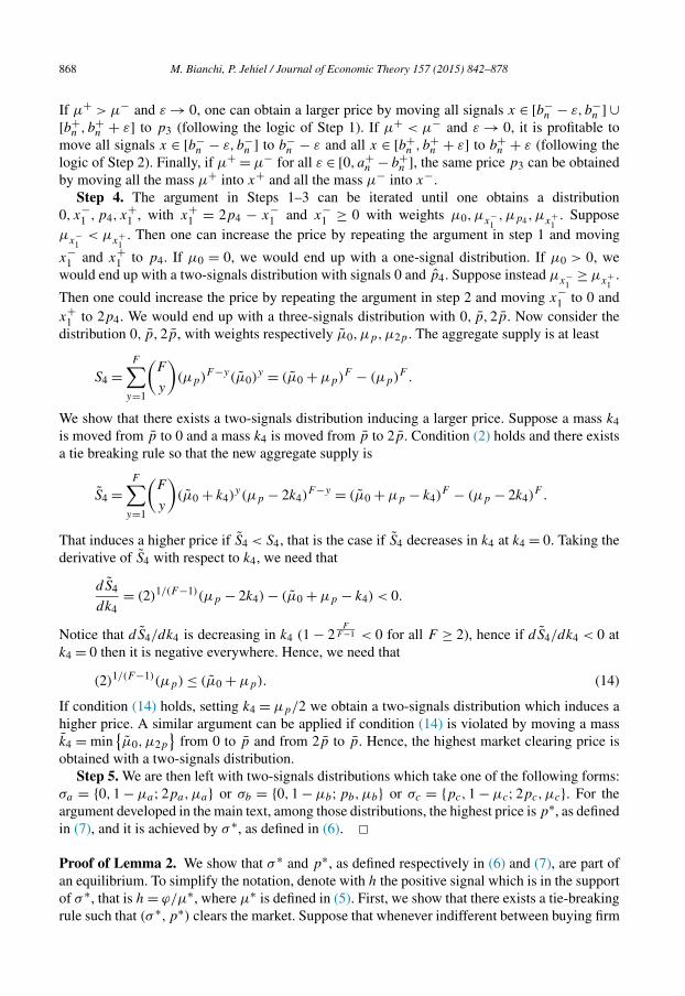
868 M. Bianchi, P. Jehiel / Journal of Economic Theory 157 (2015) 842–878
If μ+ > μ− and ε → 0, one can obtain a larger price by moving all signals x ∈ [b−n − ε, b−
n ] ∪[b+
n , b+n + ε] to p3 (following the logic of Step 1). If μ+ < μ− and ε → 0, it is profitable to
move all signals x ∈ [b−n − ε, b−
n ] to b−n − ε and all x ∈ [b+
n , b+n + ε] to b+
n + ε (following the logic of Step 2). Finally, if μ+ = μ− for all ε ∈ [0, a+
n − b+n ], the same price p3 can be obtained
by moving all the mass μ+ into x+ and all the mass μ− into x−.Step 4. The argument in Steps 1–3 can be iterated until one obtains a distribution
0, x−1 , p4, x
+1 , with x+
1 = 2p4 − x−1 and x−
1 ≥ 0 with weights μ0, μx−1, μp4, μx+
1. Suppose
μx−1
< μx+1
. Then one can increase the price by repeating the argument in step 1 and moving
x−1 and x+
1 to p4. If μ0 = 0, we would end up with a one-signal distribution. If μ0 > 0, we would end up with a two-signals distribution with signals 0 and p4. Suppose instead μx−
1≥ μx+
1.
Then one could increase the price by repeating the argument in step 2 and moving x−1 to 0 and
x+1 to 2p4. We would end up with a three-signals distribution with 0, p, 2p. Now consider the
distribution 0, p, 2p, with weights respectively μ0, μp, μ2p . The aggregate supply is at least
S4 =F∑
y=1
(F
y
)(μp)F−y(μ0)
y = (μ0 + μp)F − (μp)F .
We show that there exists a two-signals distribution inducing a larger price. Suppose a mass k4is moved from p to 0 and a mass k4 is moved from p to 2p. Condition (2) holds and there exists a tie breaking rule so that the new aggregate supply is
S4 =F∑
y=1
(F
y
)(μ0 + k4)
y(μp − 2k4)F−y = (μ0 + μp − k4)
F − (μp − 2k4)F .
That induces a higher price if S4 < S4, that is the case if S4 decreases in k4 at k4 = 0. Taking the derivative of S4 with respect to k4, we need that
dS4
dk4= (2)1/(F−1)(μp − 2k4) − (μ0 + μp − k4) < 0.
Notice that dS4/dk4 is decreasing in k4 (1 − 2F
F−1 < 0 for all F ≥ 2), hence if dS4/dk4 < 0 at k4 = 0 then it is negative everywhere. Hence, we need that
(2)1/(F−1)(μp) ≤ (μ0 + μp). (14)
If condition (14) holds, setting k4 = μp/2 we obtain a two-signals distribution which induces a higher price. A similar argument can be applied if condition (14) is violated by moving a mass k4 = min
{μ0,μ2p
}from 0 to p and from 2p to p. Hence, the highest market clearing price is
obtained with a two-signals distribution.Step 5. We are then left with two-signals distributions which take one of the following forms:
σa = {0,1 − μa;2pa,μa} or σb = {0,1 − μb;pb,μb} or σc = {pc,1 − μc;2pc,μc}. For the argument developed in the main text, among those distributions, the highest price is p∗, as defined in (7), and it is achieved by σ ∗, as defined in (6). �Proof of Lemma 2. We show that σ ∗ and p∗, as defined respectively in (6) and (7), are part of an equilibrium. To simplify the notation, denote with h the positive signal which is in the support of σ ∗, that is h = ϕ/μ∗, where μ∗ is defined in (5). First, we show that there exists a tie-breaking rule such that (σ ∗, p∗) clears the market. Suppose that whenever indifferent between buying firm
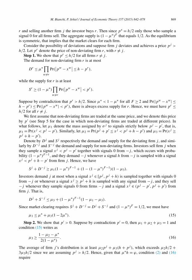
M. Bianchi, P. Jehiel / Journal of Economic Theory 157 (2015) 842–878 869
r and selling another firm j the investor buys r . Then since p∗ = h/2 only those who sample a signal 0 for all firms sell. The aggregate supply is (1 − μ∗)F that equals 1/2. As the equilibrium is symmetric, that implies that the market clears for each firm.
Consider the possibility of deviations and suppose firm j deviates and achieves a price pj >
h/2. Let pr denote the price of non-deviating firm r , with r �= j .Step 1. We show that pr ≤ h/2 for all firms r �= j .The demand for non-deviating firm r is at most
Dr ≤ μ∗ ∏w �=r
Pr(∣∣pw − xw
∣∣ ≤ h − pr),
while the supply for r is at least
Sr ≥ (1 − μ∗)∏w �=r
Pr(∣∣pw − xw
∣∣ < pr).
Suppose by contradiction that pr > h/2. Since μ∗ < 1 − μ∗ for all F ≥ 2 and Pr(|pw − xw| ≤h − pr) ≤ Pr(|pw − xw| < pr), there is always excess supply for r . Hence, we must have pr ≤h/2 for all r �= j .
We first assume that non-deviating firms are traded at the same price, and we denote this price by p′ (see Step 5 for the case in which non-deviating firms are traded at different prices). In what follows, let μ1 denote the mass assigned by σ j to signals strictly below pj − p′, that is, μ1 = Pr(xj < pj − p′). Similarly, let μ2 = Pr(pj + p′ ≤ xj < pj + h − p′) and μ3 = Pr(xj ≥pj + h − p′).
Denote by Dj and Sj respectively the demand and supply for the deviating firm j , and simi-larly by D−j and S−j the demand and supply for non-deviating firms. Investors sell firm j when they sample a signal xj < pj − p′ together with signals 0 from −j , which occurs with proba-bility (1 − μ∗)F−1, and they demand −j whenever a signal h from −j is sampled with a signal xj < pj + h − p′ from firm j . Hence, we have
Sj + D−j ≥ μ1(1 − μ∗)F−1 + (1 − (1 − μ∗)F−1)(1 − μ3).
Investors demand j at most when a signal xj ∈ [pj , pj + h) is sampled together with signals 0from −j or whenever a signal xj ≥ pj + h is sampled with any signal from −j , and they sell −j whenever they sample signals 0 from firms −j and a signal xj ∈ (pj − p′, pj + p′) from firm j . That is,
Dj + S−j ≤ μ3 + (1 − μ∗)F−1(1 − μ1 − μ3).
Since market clearing requires Sj + D−j = Dj + S−j and (1 − μ∗)F = 1/2, we must have
μ1 ≤ μ∗ + μ3(1 − 2μ∗). (15)
Step 2. We show that p′ > 0. Suppose by contradiction p′ = 0, then μ1 + μ2 + μ3 = 1 and condition (15) writes as
μ3 ≥ 1 − μ2 − μ∗
2(1 − μ∗). (16)
The average of firm j ’s distribution is at least μ2pj + μ3(h + pj ), which exceeds μ2h/2 +
3μ3h/2 since we are assuming pj > h/2. Hence, given that μ∗h = ϕ, condition (2) and (16)require

870 M. Bianchi, P. Jehiel / Journal of Economic Theory 157 (2015) 842–878
μ2
2+ 1 − μ∗ − μ2
2 (1 − μ∗)3
2< μ∗.
Since the left hand side of the above inequality decreases in μ2, the condition must be satisfied when μ2 is the largest, i.e. μ2 = 1 − μ∗ (as derived by letting μ3 = 0). The condition writes as 1 − μ∗ < 2μ∗, which is violated for all F ≥ 2. We conclude that we cannot have p′ = 0.
Step 3. The aggregate supply of all firms is at least
Sj + S−j ≥ (1 − μ2 − μ3)(1 − μ∗)F−1,
as obtained when a signal 0 from all non-deviating firms is sampled with a signal xj < pj + p′. Since market clearing requires Sj + S−j = 1/2, the previous condition requires
μ2 + μ3 ≥ μ∗. (17)
Step 4. The average of firm j ’s distribution is minimized when all signals xj < pj − p′ are concentrated at xj = 0, all signals xj ∈ [pj +p′, pj +h −p′) are concentrated at xj = pj +p′, all signals xj ≥ pj + h − p′ are concentrated at xj = pj + h − p′ and all other signals xj ∈[pj − p′, pj + p′) are concentrated at xj = pj − p′. That is, for condition (2) to hold, we need
μ2(pj + p′) + μ3(p
j + h − p′) + (1 − μ1 − μ2 − μ3)(pj − p′) ≤ ϕ. (18)
Given (15) and (17), the left hand side is minimized when μ1 = μ∗ + μ3(1 − 2μ∗) and μ2 +μ3 = μ∗. Substituting into (18), we have
(μ∗ − μ3)(pj + p′) + μ3(p
j + h − p′) + (1 − μ3)(1 − 2μ∗) (pj − p′) ≤ ϕ.
The left hand side decreases in p′ and so it is minimized when p′ = h/2. Hence, pj > h/2requires μ∗h < ϕ, which is violated since by construction μ∗h = ϕ. We conclude that there is no profitable deviation for firm j when non-deviating firms are traded at the same price p′.
Step 5. Suppose now F > 2 and non-deviating firms are traded at a different price. Suppose two non-deviating firms, say firm 1 and firm 2, are traded respectively at prices p1 and p2. Assume wlog that p1 < p2. When signal 0 from firm 1 is drawn together with signal 0 from firm 2 an investor prefers trading stock 2 (since p1 < p2) and when signal 0 from firm 1 is drawn with signal h from firm 2 an investor prefers trading stock 2 (since from Step 1 p1 < h − p2). Hence, S1 = 0 and firm 1 is not traded. We are left with a market in which F − 1 firms are traded. Suppose that, among them, the non-deviating firms are traded at the same price p. We can repeat the above argument and conclude that there is no profitable deviation. Suppose instead that among the F − 1 traded firms there exist two non-deviating firms which are traded at a different price. We can repeat the above argument and end up with F − 2 traded firms. Iterating, we end up with 2 traded firms, in which case we have already shown that there is no profitable deviation. We conclude that the profile (σ ∗, p∗) defines an equilibrium. �Proof of Proposition 6. Suppose firms choose a distribution with support on [0, 2ϕ], den-sity g symmetric around ϕ and cdfG such that [1 − 2G(x)]F−1 = 1 − x/ϕ for x < ϕ and[2G(x) − 1]F−1 = x/ϕ − 1 for x ≥ ϕ.
Step 1. Market clearing requires p = ϕ. In fact, at p = ϕ, aggregate demand is
D = F
2ϕ∫g(x)[2G(x) − 1]F−1dx = F
1
ϕ
2ϕ∫g(x)(x − ϕ)dx,
ϕ ϕ
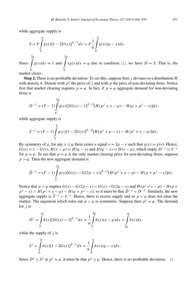
M. Bianchi, P. Jehiel / Journal of Economic Theory 157 (2015) 842–878 871
while aggregate supply is
S = F
ϕ∫0
g(x)[1 − 2G(x)]F−1dx = F1
ϕ
ϕ∫0
g(x)(ϕ − x)dx.
Since
2ϕ∫0
g(x)dx = 1 and
2ϕ∫0
xg(x)dx = ϕ due to condition (2), we have D = S. That is, the
market clears.Step 2. There is no profitable deviation. To see this, suppose firm j deviates to a distribution H
with density h. Denote with pj the price of j and with p the price of non-deviating firms. Notice first that market clearing requires p = ϕ. In fact, if p = ϕ aggregate demand for non-deviating firms is
D−j = (F − 1)
2ϕ∫ϕ
g(x)[2G(x) − 1]F−2[H(pj + x − ϕ) − H(ϕ + pj − x)]dx,
while aggregate supply is
S−j = (F − 1)
ϕ∫0
g(x)[1 − 2G(x)]F−2[H(pj + ϕ − x) − H(pj + x − ϕ)]dx.
By symmetry of g, for any x ≤ ϕ there exists a signal v = 2ϕ − x such that g(x) = g(v). Hence, G(x) = 1 − G(v), H(x − ϕ) = H(ϕ − v) and H(ϕ − x) = H(v − ϕ), which imply D−j = S−j
for p = ϕ. To see that p = ϕ is the only market clearing price for non-deviating firms, suppose p > ϕ. Then the new aggregate demand is
D−j = (F − 1)
2ϕ∫p
g(x)[G(x) − G(2p − x)]F−2[H(pj + x − p) − H(p + pj − x)]dx.
Notice that p > ϕ implies G(x) −G(2p−x) < G(x) −G(2ϕ −x) and H(pj +x −p) −H(p+pj − x) > H(pj + x − ϕ) − H(ϕ + pj − x), so it must be that D−j < D−j . Similarly, the new aggregate supply is S−j > S−j . Hence, there is excess supply and so p > ϕ does not clear the market. The argument which rules out p < ϕ is symmetric. Suppose then pj = ϕ. The demand for j is
Dj =∞∫
ϕ
h(x)[2G(x) − 1]F−1dx = 1
ϕ
2ϕ∫ϕ
h(x)(x − ϕ)dx +∞∫
2ϕ
h(x)dx,
while the supply of j is
Sj =ϕ∫
0
h(x)[1 − 2G(x)]F−1dx = 1
ϕ
ϕ∫0
h(x)(ϕ − x)dx.
Since Dj ≤ Sj at pj = ϕ, it must be that pj ≤ ϕ. Hence, there is no profitable deviation. �
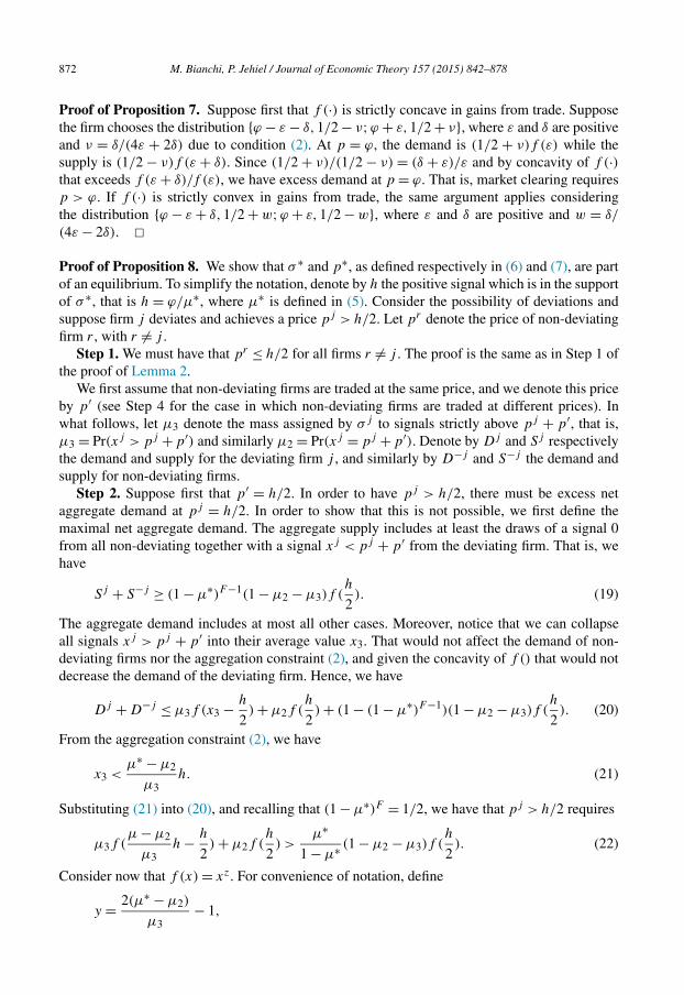
872 M. Bianchi, P. Jehiel / Journal of Economic Theory 157 (2015) 842–878
Proof of Proposition 7. Suppose first that f (·) is strictly concave in gains from trade. Suppose the firm chooses the distribution {ϕ − ε − δ,1/2 − ν;ϕ + ε,1/2 + ν}, where ε and δ are positive and ν = δ/(4ε + 2δ) due to condition (2). At p = ϕ, the demand is (1/2 + ν)f (ε) while the supply is (1/2 − ν)f (ε + δ). Since (1/2 + ν)/(1/2 − ν) = (δ + ε)/ε and by concavity of f (·)that exceeds f (ε + δ)/f (ε), we have excess demand at p = ϕ. That is, market clearing requires p > ϕ. If f (·) is strictly convex in gains from trade, the same argument applies considering the distribution {ϕ − ε + δ,1/2 + w;ϕ + ε,1/2 − w}, where ε and δ are positive and w = δ/
(4ε − 2δ). �Proof of Proposition 8. We show that σ ∗ and p∗, as defined respectively in (6) and (7), are part of an equilibrium. To simplify the notation, denote by h the positive signal which is in the support of σ ∗, that is h = ϕ/μ∗, where μ∗ is defined in (5). Consider the possibility of deviations and suppose firm j deviates and achieves a price pj > h/2. Let pr denote the price of non-deviating firm r , with r �= j .
Step 1. We must have that pr ≤ h/2 for all firms r �= j . The proof is the same as in Step 1 of the proof of Lemma 2.
We first assume that non-deviating firms are traded at the same price, and we denote this price by p′ (see Step 4 for the case in which non-deviating firms are traded at different prices). In what follows, let μ3 denote the mass assigned by σ j to signals strictly above pj + p′, that is, μ3 = Pr(xj > pj +p′) and similarly μ2 = Pr(xj = pj +p′). Denote by Dj and Sj respectively the demand and supply for the deviating firm j , and similarly by D−j and S−j the demand and supply for non-deviating firms.
Step 2. Suppose first that p′ = h/2. In order to have pj > h/2, there must be excess net aggregate demand at pj = h/2. In order to show that this is not possible, we first define the maximal net aggregate demand. The aggregate supply includes at least the draws of a signal 0from all non-deviating together with a signal xj < pj + p′ from the deviating firm. That is, we have
Sj + S−j ≥ (1 − μ∗)F−1(1 − μ2 − μ3)f (h
2). (19)
The aggregate demand includes at most all other cases. Moreover, notice that we can collapse all signals xj > pj + p′ into their average value x3. That would not affect the demand of non-deviating firms nor the aggregation constraint (2), and given the concavity of f () that would not decrease the demand of the deviating firm. Hence, we have
Dj + D−j ≤ μ3f (x3 − h
2) + μ2f (
h
2) + (1 − (1 − μ∗)F−1)(1 − μ2 − μ3)f (
h
2). (20)
From the aggregation constraint (2), we have
x3 <μ∗ − μ2
μ3h. (21)
Substituting (21) into (20), and recalling that (1 − μ∗)F = 1/2, we have that pj > h/2 requires
μ3f (μ − μ2
μ3h − h
2) + μ2f (
h
2) >
μ∗
1 − μ∗ (1 − μ2 − μ3)f (h
2). (22)
Consider now that f (x) = xz. For convenience of notation, define
y = 2(μ∗ − μ2) − 1,
μ3
M. Bianchi, P. Jehiel / Journal of Economic Theory 157 (2015) 842–878 873
and notice that x3 > h requires y > 1. Condition (22) can be written as
μ3(yh
2)z + (μ∗ − 1 + y
2μ3)(
h
2)z >
μ∗
1 − μ∗ (1 − (μ∗ − 1 + y
2μ3) − μ3)(
h
2)z,
that is(h
2
)zμ3
1 − μ∗
((y)z(1 − μ∗) − 1
2y + μ∗ − 1
2
)> 0.
Define h(y) = (y)z(1 − μ∗) − 12y + μ∗ − 1
2 and notice that h(1) = 0 and h′(y) < 0 when z(1 −μ∗) < 1/2 (in fact, h′′(y) < 0 for all z < 1 and h′(1) < 0 when z(1 −μ∗) < 1/2). Hence h(y) < 0for all y > 1 and that contradicts condition (22). That is, we cannot have pj > h/2 when p′ =h/2.
Step 3. We now show that decreasing p′ cannot increase pj . Suppose we decrease p′, say from p to p − ε, and consider the effects on the net demand for stock j . Denote with μ1 the mass of signals at pj − p, that is μ1 = Pr(xj = pj − p). Investors who sample xj = pj − p
together with signal 0 from all other firms now strictly prefer selling firm j . Hence, the supply Sj increases by μ1(1 − μ∗)F−1(1 − 1
F). Consider the effects on the demand Dj . If σ j assigns
positive mass to xj = h + pj − p, investors who sample xj = h + pj − p with a signal h from any other firm −j now strictly prefer not to buy firm j . That pushes the demand Dj down. If σ j assigns positive mass to xj = pj + p, investors who sample xj = pj + p with signal 0 from all other firms −j now strictly prefer to buy firm j . However, that does not affect the demand Dj since the tie-breaking rule supporting the equilibrium in (6) and (7) already assigned all the demand to firm j . Finally, notice that it is never optimal that σj assigns positive mass to signals in (pj , pj + p). Those signals can be decreased to pj as that would not affect the demand of any firm while at the same time allowing to increase all the other signals in σ j and satisfy the aggregation condition (2). Hence, decreasing p′ involves no change in the demand due to signals slightly below pj + p. Hence, the demand Dj cannot increase as we decrease p′. It follows that Dj − Sj cannot increase and, given that the price pj is a smooth function of the net demand Dj − Sj , pj cannot increase as we decrease p′. That shows that we cannot have pj > h/2 when p′ ≤ h/2.
Step 4. Suppose now F > 2 and non-deviating firms are traded at a different price. The argu-ment to rule out that this cannot help the deviating firm is the same as in Step 5 of the proof of Lemma 2. We conclude that the profile (σ ∗, p∗) is part of an equilibrium. �Proof of Proposition 9. Suppose that Xj ∈ [0, H ] and let μ∗ = 1 − (1/2)1/F . If ϕ/μ∗ ≤ H , the upper bound does not bind and the analysis of Proposition 2 applies. Suppose instead ϕ/
(1 − μ∗) ≥ H . In this case, one can obtain a price p = H with the distribution σ = {0, 1 − η;H, η} in which (η)F ≥ 1/2, that is η ≥ 1 − μ∗. Since ϕ ≥ (1 − μ∗)H , condition (2) is satisfied. This is obviously the highest price irrespective of F . Hence, in what follows, we focus on
H ∈ (ϕ
1 − μ∗ ,ϕ
μ∗ ). (23)
We first show that if H ≥ H , as defined by condition (10), the highest market clearing price is achieved with σH = {(ϕ − μ∗H)/(1 − μ∗),1 − μ∗;H,μ∗} and it is defined as in (11) by
pH = 1(H + ϕ − μ∗H
∗ ). (24)
2 1 − μ
874 M. Bianchi, P. Jehiel / Journal of Economic Theory 157 (2015) 842–878
By the same argument a the one developed in Lemma 1, the highest market clearing price is obtained when the distribution takes one of the following forms. Either, σa = {0,1 − μa;pa,μa}with (μa)
F ≥ 1/2 and so the highest price is obtained when μa = 1 − μ∗ and it writes as
pa = ϕ
1 − μ∗ . (25)
The price defined in (24) exceeds pa in (25) if
H ≥ ϕ
1 − 2μ∗ . (26)
Or σb = {0, μ, l,1 − μb − μ;H,μb} with pb = (H + l)/2 and because of market clearing
1 − (1 − μ)F + (1 − μb − μ)F = 1/2. (27)
Differently from Lemma 1, it may be optimal to have μ > 0 since shifting signals l and H further away from the price is not feasible. Since σH is obtained as a special case of σb when μ = 0, we investigate under which condition pb is maximized by μ = 0. Given the market clearing condition (27), l is defined by condition (2) and so we have
pb = 1
2(H + ϕ − (1 − μ − ((1 − μ)F − 1
2 )1F )H
((1 − μ)F − 12 )
1F
). (28)
Differentiating pb with respect to μ, we see that pb decreases in μ if
2ϕ − H ≤ 0. (29)
That is, under condition (29), pb is maximized by μ = 0. Hence, if conditions (26) and (29) are satisfied, as required by condition (10) in the text, the highest market clearing price is defined by (24). This price increases in F since μ∗ decreases in F .
We now show that pH can be sustained in equilibrium. The logic follows closely the proof of Lemma 2. Suppose firm j deviates and achieves a price pj > (H + l)/2 and let pr denote the price of non-deviating firm r , with r �= j .
Step 1. Following the same argument as the one in Step 1 of the proof of Lemma 2, we must have pr ≤ (H + l)/2 for all r �= j or there would be excess supply for firm r .
We first assume that non-deviating firms are traded at the same price, and we denote it with p′ (see Step 5 for the case in which non-deviating firms are traded at different prices). Let μ0 =Pr(xj < pj + p′ − H); μ1 = Pr(pj + p′ − H ≤ xj < pj − p′ + l), and μ2 = Pr(pj + p′ − l ≤xj ≤ H).
Following the logic of Lemma 2, we have that market clearing requires
μ0 + μ1 ≤ μ∗. (30)
Step 2. We show that p′ > l. Suppose by contradiction that p′ = l, then μ0 + μ1 + μ2 = 1and (30) writes as
μ2 ≥ 1 − μ∗. (31)
The average of firm j ’s distribution is at least μ2pj , and so given (31) and pj > (H + l)/2,
condition (2) requires
(1 − μ∗)(H + l) < 2ϕ,
that is, H + ϕ − 2Hμ∗ < 2ϕ, and that violates (26). We conclude that we cannot have p = l.
M. Bianchi, P. Jehiel / Journal of Economic Theory 157 (2015) 842–878 875
Step 3. Following the logic of Step 3 in the proof of Lemma 2, we need
μ2 ≥ μ∗ + μ0(1 − 2μ∗), (32)
or we would have excess aggregate supply.Step 4. Condition (2) requires
μ1(pj + p′ − H) + μ2(p
j + p′ − l) + (1 − μ0 − μ1 − μ2)(pj − p′ + l) ≤ ϕ. (33)
The previous expression is linear in p′, so it must hold either for p′ = (H + l)/2 or for p′ → l. Suppose p′ = (H + l)/2, we must have μ2H + (1 − μ0 − μ2)l < ϕ, which given (30) and (32) must hold when μ0 = μ∗ − μ1 and μ2 = μ∗ + (μ∗ − μ1)(1 − 2μ∗). That is, we need (μ∗ − μ1) (H − 2l − 2Hμ∗ + 2lμ∗) < 0, which is equivalent to H < 2ϕ, and that violates con-dition (29). Suppose instead p′ → l, (33) requires (1 − μ0 − μ1)(H + l) < 2ϕ, which given (30)requires (1 − μ∗)(H + l) < 2ϕ. As shown in Step 2, this violates (26).
Step 5. The argument to show that there are no profitable deviations when some non-deviating firms are traded at a different price follows Step 5 of the proof of Lemma 2. �Proof of Proposition 10. Suppose firm j has fundamental ϕj = ϕ + εj , σ j = {εj , 1 − μ∗;2p∗ + εj , μ∗} and prices are pj = p∗ + εj . The logic to show that the market clears is the same as in Lemma 2. Let h = ϕ/μ∗, where μ∗ = 1 − (1/2)1/F , and suppose firm j deviates and achieves a price pj > h/2 + εj . Let pr denote the price of non-deviating firm r , with r �= j .
Step 1. Following the argument of Step 1 in the proof of Lemma 2, we establish that pr ≤h/2 + εr for all r �= j as otherwise there would be excess supply for firm r .
Assume first that the price of the non-deviating firms takes the following form:
pr = εr + λh for all r �= j,
where, due to Step 1, λ ≤ 1/2. In Step 5, we consider the general case in which pr = εr + λrh. Let μ0 = Pr(xj < pj − (1 −λ)h); μ1 = Pr(pj − (1 −λ)h ≤ xj < pj −λh); μ2 = Pr(pj +λh ≤xj < pj + (1 − λ)h); and μ3 = Pr(xj ≥ pj + (1 − λ)h).
Following the logic of Lemma 2, we have that market clearing requires
μ0 + μ1 ≤ μ∗ + μ3(1 − 2μ∗). (34)
Step 2. We show that λ > 0 when F > 2.Suppose by contradiction that λ = 0 and so μ0 + μ1 + μ2 + μ3 = 1. Hence, (34) writes as
μ3 ≥ 1 − μ2 − μ∗
2(1 − μ∗). (35)
The average of firm j ’s distribution is at least μ1(pj − h) + μ2p
j + μ3(h + pj ), which exceeds μ1(ε
j − h/2) + μ2(h/2 + εj ) + μ3(3h/2 + εj ) since we are assuming pj > h/2 + εj . Suppose first εj < h/2. Conditions (2) and (35) require
μ2(h
2+ εj ) + (
1 − μ2 − μ∗
2(1 − μ∗))(
3h
2+ εj ) < ϕ + εj . (36)
Since the left hand side of the above inequality decreases in μ2, it must be satisfied when μ2is the largest. Substituting μ2 = 1 − μ∗ and ϕ = μ∗h into (36), we have h (1 − 3μ∗) < 2μ∗εj , which is violated for all F > 2. A similar argument applies when εj ≥ h/2 by noticing that the average of firm j ’s distribution is minimized when μ2 = 1 − μ∗ and so in particular we must
876 M. Bianchi, P. Jehiel / Journal of Economic Theory 157 (2015) 842–878
have (1 − μ∗)h/2 < μ∗(h + εj ). Given (12), that requires (1 − μ∗)h/2 < μ∗(h + (1 − 2μ∗)h), which is violated for any F > 2. We conclude that we cannot have λ = 0 when F > 2.
Step 3. Suppose λ > 0. The aggregate supply of all firms is at least
Sj + S−j ≥ μ0 + (1 − μ2 − μ3 − μ0)(1 − μ∗)F−1,
as obtained when a signal xj < pj − (1 −λ)h from firm j is sampled with any other signal from firms −j and when a signal εr from all firms r �= j is sampled with a signal xj < pj + λh from firm j . Hence, market clearing requires
μ2 + μ3 ≥ μ∗ + μ0(1 − 2μ∗). (37)
Step 4. Condition (2) requires
μ1(pj − (1 − λ)h) + μ2(p
j + λh) + μ3(pj + (1 − λ)h)
+ (1 − μ0 − μ1 − μ2 − μ3)(pj − λh) ≤ ϕ + εj . (38)
Suppose first F > 2 and so λ > 0. Given (34) and (37), the left hand side is minimized when μ1 = μ∗ + μ3(1 − 2μ∗) − μ0 and μ2 = μ∗ + μ0(1 − 2μ∗) − μ3. Substituting into (38), we see that the left hand side of (38) decreases in λ and so it must hold when λ = 1/2. This in turn requires εj > (1 − 2μ∗)h, which violates condition (12) in the text.
Suppose finally that F = 2. The left hand side of inequality (38) is linear in λ, so it must hold either for λ = 1/2 or for λ = 0. If λ = 1/2, we can repeat the argument above and conclude that εj > (1 − 2μ∗)h violates condition (12) in the text (notice that 2(p∗ − ϕ) = ϕ
√2 when F = 2
and so εj ≤ ϕ√
2/2 implies εj ≤ 2(p∗ − ϕ)). Suppose then λ = 0. Condition (38) requires in particular μ2p
j + μ3(pj + h) ≤ ϕ + εj , which given (35) requires
μ2pj + 1 − μ2 − μ∗
2(1 − μ∗)(pj + h) ≤ ϕ + εj .
The left hand side is linear in μ2 and so it must hold when either μ2 = 0 or μ2 = 1 −μ∗. Suppose μ2 = 0, we have pj ≤ 2εj − (1 − 2μ∗)h, that implies pj < h/2 + εj since by condition (12)εj ≤ ϕ
√2/2. Suppose then μ2 = 1 − μ∗, we have pj ≤ (ϕ + εj )/(1 − μ∗). Condition (12) is
equivalent to (ϕ + εj )/(1 − μ∗) ≤ h/2 + εj . We conclude that there is no profitable deviation for firm j when non-deviating firms are traded at prices pr = εr + λh.
Step 5. Suppose each non-deviating firm is traded at a price pr = εr + λrh. The argument to show that there are no profitable deviations follows Step 5 of the proof of Lemma 2. �References
[1] E. Albagli, C. Hellwig, A. Tsyvinski, A theory of asset prices based on heterogeneous information, Mimeo, 2012.[2] W. Bailey, H. Li, C.X. Mao, R. Zhong, Regulation fair disclosure and earnings information: market, analyst, and
corporate responses, J. Finance 58 (6) (2003) 2487–2514.[3] G. Baquero, M. Verbeek, Do sophisticated investors believe in the law of small numbers? Mimeo, 2008.[4] N. Barberis, A. Shleifer, R. Vishny, A model of investor sentiment, J. Finan. Econ. 49 (3) (1998) 307–343.[5] W.H. Beaver, The information content of annual earnings announcements, J. Acc. Res. 6 (1968) 67–92.[6] S. Benartzi, Excessive extrapolation and the allocation of 401(k) accounts to company stock, J. Finance 56 (5)
(2001) 1747–1764.[7] D. Bergstresser, T. Philippon, CEO incentives and earnings management, J. Finan. Econ. 80 (3) (2006) 511–529.[8] P. Bordalo, N. Gennaioli, A. Shleifer, Salience theory of choice under risk, Quart. J. Econ. 127 (3) (2012)
1243–1285.[9] N. Burns, S. Kedia, The impact of performance-based compensation on misreporting, J. Finan. Econ. 79 (1) (2006)
35–67.

M. Bianchi, P. Jehiel / Journal of Economic Theory 157 (2015) 842–878 877
[10] R. Chahrour, Public communication and information acquisition, Amer. Econ. J. Macroecon. 6 (3) (2014) 73–101.[11] S. Chen, M.L. DeFond, C.W. Park, Voluntary disclosure of balance sheet information in quarterly earnings an-
nouncements, J. Acc. Econ. 33 (2) (2002) 229–251.[12] M.M. Cornett, A.J. Marcus, H. Tehranian, Corporate governance and pay-for-performance: the impact of earnings
management, J. Finan. Econ. 87 (2) (2008) 357–373.[13] V.P. Crawford, J. Sobel, Strategic information transmission, Econometrica 50 (6) (1982) 1431–1451.[14] J.B. De Long, A. Shleifer, L.H. Summers, R.J. Waldmann, Noise trader risk in financial markets, J. Polit. Economy
98 (4) (1990) 703–738.[15] J.B. De Long, A. Shleifer, L.H. Summers, R.J. Waldmann, Positive feedback investment strategies and destabilizing
rational speculation, J. Finance 45 (2) (1990) 379–395.[16] M. Di Maggio, M. Pagano, Financial disclosure with limited processing capacity, Mimeo, 2013.[17] J. Dominitz, C.F. Manski, Measuring and interpreting expectations of equity returns, J. Appl. Econometrics 26 (3)
(2011) 352–370.[18] J. Efendi, A. Srivastava, E.P. Swanson, Why do corporate managers misstate financial statements? the role of option
compensation and other factors, J. Finan. Econ. 85 (3) (2007) 667–708.[19] M.J. Eppler, J. Mengis, The concept of information overload: a review of literature from organization science,
accounting, marketing, mis, and related disciplines, Inf. Soc. 20 (5) (2004) 325–344.[20] E. Eyster, M. Piccione, An approach to asset pricing under incomplete and diverse perceptions, Econometrica 81 (4)
(2013) 1483–1506.[21] M.J. Flannery, S.H. Kwan, M. Nimalendran, Market evidence on the opaqueness of banking firms’ assets, J. Finan.
Econ. 71 (3) (2004) 419–460.[22] J. Francis, K. Schipper, L. Vincent, Expanded disclosures and the increased usefulness of earnings announcements,
Acc. Rev. 77 (3) (2002) 515–546.[23] D. Fudenberg, J. Tirole, A theory of income and dividend smoothing based on incumbency rents, J. Polit. Economy
103 (1) (1995) 75–93.[24] X. Gabaix, A sparsity-based model of bounded rationality, with application to basic consumer and equilibrium
theory, Quart. J. Econ. 129 (4) (2014) 1661–1710.[25] R. Greenwood, S. Nagel, Inexperienced investors and bubbles, J. Finan. Econ. 93 (2) (2009) 239–258.[26] R. Greenwood, A. Shleifer, Expectations of returns and expected returns, Rev. Finan. Stud. 27 (3) (2014) 714–746.[27] S.J. Grossman, The informational role of warranties and private disclosure about product quality, J. Law Econ.
24 (3) (1981) 461–483.[28] S.J. Grossman, J.E. Stiglitz, On the impossibility of informationally efficient markets, Amer. Econ. Rev. 70 (3)
(1980) 393–408.[29] F. Gul, W. Pesendorfer, T. Strzalecki, Behavioral competitive equilibrium and extreme prices, Mimeo, 2011.[30] J.M. Harrison, D.M. Kreps, Speculative investor behavior in a stock market with heterogeneous expectations, Quart.
J. Econ. 92 (2) (1978) 323–336.[31] D. Hirshleifer, S.S. Lim, S.H. Teoh, Driven to distraction: extraneous events and underreaction to earnings news,
J. Finance 64 (5) (2009) 2289–2325.[32] D. Hirshleifer, S.H. Teoh, Limited attention, information disclosure, and financial reporting, J. Acc. Econ. 36 (1–3)
(2003) 337–386.[33] H. Hong, J. Scheinkman, W. Xiong, Advisors and asset prices: a model of the origins of bubbles, J. Finan. Econ.
89 (2) (2008) 268–287.[34] H. Hong, J.C. Stein, Disagreement and the stock market, J. Econ. Perspect. 21 (2) (2007) 109–128.[35] O.-K. Hope, W.B. Thomas, G. Winterbotham, Geographic earnings disclosure and trading volume, J. Acc. Public
Policy 28 (3) (2009) 167–188.[36] P. Jehiel, Analogy-based expectation equilibrium, J. Econ. Theory 123 (2) (2005) 81–104.[37] P. Jehiel, On transparency in organizations, Rev. Econ. Stud. (2015), http://dx.doi.org/10.1093/restud/rdu040, forth-
coming.[38] K.L. Judd, The law of large numbers with a continuum of IID random variables, J. Econ. Theory 35 (1) (1985)
19–25.[39] D. Kahneman, Thinking, Fast and Slow, Farrar, Straus and Giroux, 2011.[40] E. Kamenica, M. Gentzkow, Bayesian persuasion, Amer. Econ. Rev. 101 (6) (2011) 2590–2615.[41] E. Kandel, N.D. Pearson, Differential interpretation of public signals and trade in speculative markets, J. Polit.
Economy 103 (4) (1995) 831–872.[42] B. Koszegi, A. Szeidl, A model of focusing in economic choice, Quart. J. Econ. 128 (1) (2013) 53–104.[43] A. Levitt, The numbers game, Remarks delivered at the NYU Center for Law and Business, September 28, 1998.

878 M. Bianchi, P. Jehiel / Journal of Economic Theory 157 (2015) 842–878
[44] P. Milgrom, Good news and bad news: representation theorems and applications, Bell J. Econ. 12 (2) (1981) 380–391.
[45] P. Milgrom, N. Stokey, Information, trade and common knowledge, J. Econ. Theory 26 (1) (1982) 17–27.[46] D.P. Morgan, Rating banks: risk and uncertainty in an opaque industry, Amer. Econ. Rev. 92 (4) (2002) 874–888.[47] M.J. Osborne, A. Rubinstein, Games with procedurally rational players, Amer. Econ. Rev. 88 (4) (1998) 834–847.[48] T.A. Paredes, Blinded by the light: information overload and its consequences for securities regulation, Wash. Univ.
Law Quart. 81 (2003) 417.[49] A. Pavan, Attention, coordination, and bounded recall, Mimeo, 2014.[50] M. Rabin, Inference by believers in the law of small numbers, Quart. J. Econ. 117 (3) (2002) 775–816.[51] M. Rabin, D. Vayanos, The gambler’s and hot-hand fallacies: theory and applications, Rev. Econ. Stud. 77 (2) (2010)
730–778.[52] L. Rayo, I. Segal, Optimal information disclosure, J. Polit. Economy 118 (5) (2010) 949–987.[53] A. Rubinstein, R. Spiegler, Money pumps in the market, J. Eur. Econ. Assoc. 6 (1) (2008) 237–253.[54] A. Sarkar, R.A. Schwartz, Market sidedness: insights into motives for trade initiation, J. Finance 64 (1) (2009)
375–423.[55] J.A. Scheinkman, W. Xiong, Heterogeneous beliefs, speculation and trading in financial markets, in: R.A. Car-
mona, E. Çinlar, I. Ekeland, E. Jouini, J.A. Scheinkman, N. Touzi (Eds.), Paris–Princeton Lectures on Mathematical Finance 2003, Springer, Berlin/Heidelberg, 2004, pp. 223–233.
[56] R.J. Shiller, Measuring bubble expectations and investor confidence, J. Psychol. Financ. Mark. 1 (1) (2000) 49–60.[57] H.S. Shin, Disclosures and asset returns, Econometrica 71 (1) (2003) 105–133.[58] C.A. Sims, Implications of rational inattention, J. Monet. Econ. 50 (3) (2003) 665–690.[59] R. Spiegler, Competition over agents with boundedly rational expectations, Theor. Econ. 1 (2) (2006) 207–231.[60] R. Spiegler, The market for quacks, Rev. Econ. Stud. 73 (4) (2006) 1113–1131.[61] J.C. Stein, Efficient capital markets, inefficient firms: a model of myopic corporate behavior, Quart. J. Econ. 104 (4)
(1989) 655–669.[62] J. Steiner, C. Stewart, Price distortions in high-frequency markets, Mimeo, 2012.[63] A. Tversky, D. Kahneman, Belief in the law of small numbers, Psychol. Bull. 76 (2) (1971) 105–110.[64] R.E. Verrecchia, Essays on disclosure, J. Acc. Econ. 32 (1–3) (2001) 97–180.