financial model calibration using consistency hints...

IEEE TRANSACTIONS ON NEURAL NETWORKS, VOL. 12, NO. 4, JULY 2001 791

Financial Model Calibration Using Consistency HintsYaser S. Abu-Mostafa

Abstract—We introduce a technique for forcing the calibrationof a financial model to produce valid parameters. The techniqueis based on learning from hints. It converts simple curve fittinginto genuine calibration, where broad conclusions can be inferredfrom parameter values. The technique augments the error functionof curve fitting with consistency hint error functions based on theKullback–Leibler distance. We introduce an efficient EM-type op-timization algorithm tailored to this technique. We also introduceother consistency hints, and balance their weights using canonicalerrors. We calibrate the correlated multifactor Vasicek model of in-terest rates, and apply it successfully to Japanese Yen swaps marketand U.S. Dollar yield market.

Index Terms—Canonical error, computational finance, consis-tency hint, cross entropy, EM algorithm, financial engineering, in-terest rates, Kullback–Leibler distance, model calibration, multi-factor models, optimization, overfitting, Vasicek model, volatilityterm structure.

I. INTRODUCTION

T HE calibration of a financial model is the process of tuningthe model parameters to fit market data. Unlike the param-

eters of generic learning models such as neural networks, theparameters of financial models correspond to economic and fi-nancial quantities. For instance, they might correspond to thevolatility of a given market, or to the steady-state interest rate.These semantic aspects of the parameters are often lost in theprocess of “curve fitting.” We may end up with a good fit thatnonetheless assigns improbable or contradictory values to theparameters. For instance, we may fit the prices of bonds verywell, only to find that a volatility parameter in the formula isfive times what it should be. Such an inconsistency needs tobe avoided since the plausibility of the solution depends on theplausibility of the model it is based on.

In order to force the calibration process to conform with thecharacteristics of the model parameters, we will supplement itwith consistencyhints about these parameters. Hints [2], [3]are the auxiliary pieces of information appended to the data tohelp direct the learning process toward more plausible solutions.Consistency hints can have a dramatic impact on the calibra-tion. A case in point is illustrated in Figs. 1 and 2. Fig. 1 showsthe results of fitting market data with and without consistencyhints. Both fits appear to be equally good, and the hints do notseem to make a difference. However, a huge difference is shown

Manuscript received December 30, 2000; revised March 26, 2001. This workwas supported by the Center for Neuromorphic Systems Engineering, an Engi-neering Research Center supported by the National Science Foundation underNSF Cooperative Agreement EEC 9402726.

The author is with the Learning Systems Group, Departments of ElectricalEngineering, Computer Science, and Computation and Neural Systems, Cali-fornia Institute of Technology, Pasadena, CA 91125 USA.

Publisher Item Identifier S 1045-9227(01)05017-2.

in Fig. 2. Using the parameter values from the two calibrationsof Fig. 1, we computed the market volatility implied by theseparameters. When the hints are used, the volatility is in almostperfect agreement with the historical value it is meant to predict.When the hints are not used, the volatility is completely off. Thiscontrast could not have been detected by comparing the two fitsof Fig. 1, on which the calibrations were based.

Hints were first introduced in the context of neural networks[1] to reduce overfitting, which results from having too manyweights [12]. Such redundancy allows the learning algorithmto fit idiosyncrasies of the training data that have nothing todo with the function being learned. Inconsistency in calibrationis a manifestation of overfitting, too. As we saw in Fig. 1, wecan fit the same set of market data with different sets of param-eters, some consistent and some not. This means that the pa-rameters are redundant, and therefore susceptible to overfitting.Since hints must always be valid properties in the context theyare used, they will steer the fit toward the more consistent solu-tion.

The calibration of complex models is more prone to over-fitting than that of simple models, since complex models havemore parameters that can be exploited in the fit. Without tech-niques such as consistency hints, complex models may have tobe avoided altogether because of this drawback. However, thesecomplex models are needed to explain the behavior of finan-cial markets more accurately. For instance, multi-factor interestrate models are more realistic in representing the behavior of in-terest rates than single-factor models. Consistency hints imposean increasingly tighter constraint on higher-order models, thusregulating the overfitting potential proportionately.

Depending on the application, the use of consistency hintsmay be crucial to the final results. Although the calibrationis concerned with fitting market data, we are not just after agood fit, but also acorrect fit. The fit may be only a means toinfer other quantities, such as the volatility of Fig. 2. The fitmay also be used to help a specific application, such asrela-tive-value trading, which is based on whether the model predic-tion is higher or lower than the current market value. Even fortwo equally good fits like those of Fig. 1, this prediction can bedifferent. For instance, the model prediction of the 15-year parrate is higher than the market value when hints are used, but it isabout the same as the market value when hints are not used. Ifwe are going to base a trade on the model prediction, we musthave a reason to believe that one fit or the other is more credible,beyond just being a good-looking fit.

To describe how consistency hints are used in financial modelcalibration, we will consider a multi-factor interest rate model.Section II introduces this model and develops the basic frame-work for calibration. Section III defines consistency hints andderives the formulas that quantify the hint errors. Section IV

1045–9227/01$10.00 © 2001 IEEE

792 IEEE TRANSACTIONS ON NEURAL NETWORKS, VOL. 12, NO. 4, JULY 2001

(a)

(b)

Fig. 1. The results of calibrating a financial model to swaps market data, with and without consistency hints. The two fits are virtually indistinguishable. (a)Fitting swap par rates without hints. (b) Fitting swap par rates with hints.

discusses implementation issues and experimental results. Sec-tion V takes a look at calibration from a probabilistic point ofview, and provides a more principled framework for our tech-niques, including the introduction of canonical errors. Finally,for self sufficiency, the Appendix provides brief mathematicalderivations for the main functions of the interest rate model weuse.

II. THE INTEREST-RATE MODEL

Interest-rate models are among the more sophisticated finan-cial models, and their calibration is quite challenging. We aregoing to use the Vasicek model for interest rates [14], [18] as aparadigm for employing consistency hints in the calibration offinancial models. This concrete example will enable us to do afull derivation of the consistency hint equations and to illustratethe numerical results using real-life data. It is fairly straightfor-ward to adapt our method to the calibration of other interest-ratemodels that have analytic solutions, as well as to analogous fi-nancial models that deal with other markets.

A. Vasicek Model

The premise of the Vasicek model is that the evolution ofinterest rates in time is driven by two forces. The first is a ‘drift’toward a steady-state or equilibrium value of what the interestrate should be. The second is an injection of random movementsinto the interest rate as a result of the unpredictable economicenvironment. How these two forces interact is what defines aVasicek model.

In its simplest form, the model uses a steady-state interest rate, a speed of converging to that steady state, and a volatility

or “randomness level” , to describe the instantaneous interestrate as a function governed by the equation

where is the infinitesimal increment in time, and is an in-finitesimal stochastic variable ( is formally a Wiener process).The drift element is captured by the portion of ,and indeed this term pushestoward . If , this term

ABU-MOSTAFA: FINANCIAL MODEL CALIBRATION USING CONSISTENCY HINTS 793

(a)

(b)

Fig. 2. The volatility term structure of forward rates (6 months to 20 years) corresponding to the fits of Fig. 1. (a) Historical versus theoretical volatility withouthints. (b) Historical versus theoretical volatility with hints. In spite of those fits being almost identical, the theoretical volatility in (a) is in gross violation of thehistorical volatility it is supposed to predict, while in (b) they are in almost perfect agreement. Consistency hints are not used in (a), but used in (b).

is negative, hence will drift downwards toward , while if, this term is positive hence will drift upwards, again

toward . The value of modulates the change that results inthis drift, and hence determines the speed of converging to thesteady state. The portion of adds the random com-ponent to the interest rate.accumulates the different ’sthat occur as time goes by, but this accumulated random compo-nent is subject to decaying asdrifts toward by virtue of the

term. Fig. 3 shows an evolution of the instantaneousinterest rate under this model.

The focus of this paper is not the stochastic differential equa-tion (SDE) itself, but the functions of interest rate that are de-rived from the SDE. The parameters of the SDE will appear inthe expressions of these functions (see the Appendix), and whenthe functions are calibrated to market data, the values of the pa-rameters are determined. The understanding of what these pa-rameters signify and how they interact is important to appreciatehow consistency hints come into play.

With this in mind, let us illustrate the more general form ofthe Vasicek model. This form is called the multifactor modelbecause it asserts that the interest rate is not just a singleas inthe above equation, but rather a superposition of several’s ofanalogous form. These’s are the “factors,” and each of themfollows the same basic equation. Thus,

for where is the number of factors. The interestrate is given by the sum of these factors

The philosophy behind having multiple factors stems fromthe observation that there are different time scales for the be-havior of interest rates. Some aspects of this behavior are ob-served in a short time horizon (high-speed factors or large),


Fig. 3. Simulation of instantaneous interest rates under the Vasicek model. Two scenarios with different volatilities are presented for the same steady-state rateof 6%, and the same mean reversion speed.

and some aspects are observed in a longer horizon (low-speedfactors or small ). Each factor has its own steady-stateandits own volatility . The corresponding stochastic elements

are not always independent, hence there are correlationcoefficients between and as part of the model pa-rameters. The model is sometimes referred to as acorrelatedmulti-factor Vasicek.

It is obvious that the multi-factor model provides more flex-ibility for fitting the data by introducing more parameters thatcan be exploited in the calibration process. Therefore, a 3-factorVasicek model is more powerful than a 2-factor Vasicek model.By the same token, the 3-factor Vasicek model will be moreprone to overfitting, i.e., to fitting the idiosyncrasies of a par-ticular data set at the expense of proper generalization to newdata, because it has more resources for such a fit. This problemlimits the number of factors that can be used in practice, evenif more factors are needed to model real markets. Multifactormodels need techniques like the ones we are introducing in thispaper to be reliably calibrated. Consistency hints constrain themultitude of parameters in these models so as to keep overfit-ting in check. The constraining is based on legitimate rules thatmay be inadvertently violated if the calibration is done withoutthe hints.

B. Calibration

We now address how the Vasicek model is used to fit marketdata, or, equivalently, how market data is used to calibrate the

Vasicek model. Let denote the vector of all the parametersin the Vasicek -factor model. A market function related tointerest rates, be it the price of a 30-year bond or the yieldof three-month CD, will have a theoretical value based on themodel that is function of , say . It will also have an actualvalue observed in the market, say. If the model is correct, andthe value of is chosen properly, we would have

Since the model is not perfect, we have to settle for athat comes closest to the above equation. For instance, we canpick the value of that minimizes the error function

If we have several market functions , say theprices of bonds of different maturities, we can minimize

Variations of this error measure are of course possible. Wewill refer to this error as thefit error, as distinct from thecon-sistency errorto be introduced in Section III.

Calibrating the model to market data is the process of de-termining that minimizes the error. It is no different fromcomputing the weights of a neural network by minimizing theerror between the network prediction and the actual data, except


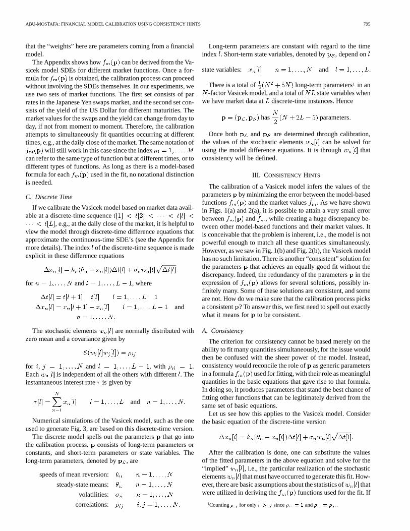
that the “weights” here are parameters coming from a financialmodel.

The Appendix shows how can be derived from the Va-sicek model SDEs for different market functions. Once a for-mula for is obtained, the calibration process can proceedwithout involving the SDEs themselves. In our experiments, weuse two sets of market functions. The first set consists of parrates in the Japanese Yen swaps market, and the second set con-sists of the yield of the US Dollar for different maturities. Themarket values for the swaps and the yield can change from day today, if not from moment to moment. Therefore, the calibrationattempts to simultaneously fit quantities occurring at differenttimes, e.g., at the daily close of the market. The same notation of

will still work in this case since the indexcan refer to the same type of function but at different times, or todifferent types of functions. As long as there is a model-basedformula for each used in the fit, no notational distinctionis needed.

C. Discrete Time

If we calibrate the Vasicek model based on market data avail-able at a discrete-time sequence

, e.g., at the daily close of the market, it is helpful toview the model through discrete-time difference equations thatapproximate the continuous-time SDE’s (see the Appendix formore details). The indexof the discrete-time sequence is madeexplicit in these difference equations

for and , where

and

The stochastic elements are normally distributed withzero mean and a covariance given by

for , and , with .Each is independent of all the others with different. Theinstantaneous interest rateis given by

and

Numerical simulations of the Vasicek model, such as the oneused to generate Fig. 3, are based on this discrete-time version.

The discrete model spells out the parametersthat go intothe calibration process. consists of long-term parameters orconstants, and short-term parameters or state variables. Thelong-term parameters, denoted by, are

speeds of mean reversion:

steady-state means:

volatilities:

correlations:

Long-term parameters are constant with regard to the timeindex . Short-term state variables, denoted by, depend on

state variables: and

There is a total of long-term parameters1 in an-factor Vasicek model, and a total of state variables when

we have market data atdiscrete-time instances. Hence

has parameters

Once both and are determined through calibration,the values of the stochastic elements can be solved forusing the model difference equations. It is through thatconsistency will be defined.

III. CONSISTENCYHINTS

The calibration of a Vasicek model infers the values of theparameters by minimizing the error between the model-basedfunctions and the market values . As we have shownin Figs. 1(a) and 2(a), it is possible to attain a very small errorbetween and , while creating a huge discrepancy be-tween other model-based functions and their market values. Itis conceivable that the problem is inherent, i.e., the model is notpowerful enough to match all these quantities simultaneously.However, as we saw in Fig. 1(b) and Fig. 2(b), the Vasicek modelhas no such limitation. There is another “consistent” solution forthe parameters that achieves an equally good fit without thediscrepancy. Indeed, the redundancy of the parametersin theexpression of allows for several solutions, possibly in-finitely many. Some of these solutions are consistent, and someare not. How do we make sure that the calibration process picksa consistent ? To answer this, we first need to spell out exactlywhat it means for to be consistent.

A. Consistency

The criterion for consistency cannot be based merely on theability to fit many quantities simultaneously, for the issue wouldthen be confused with the sheer power of the model. Instead,consistency would reconcile the role ofas generic parametersin a formula used for fitting, with their role as meaningfulquantities in the basic equations that gave rise to that formula.In doing so, it produces parameters that stand the best chance offitting other functions that can be legitimately derived from thesame set of basic equations.

Let us see how this applies to the Vasicek model. Considerthe basic equation of the discrete-time version

After the calibration is done, one can substitute the valuesof the fitted parameters in the above equation and solve for the“implied” , i.e., the particular realization of the stochasticelements that must have occurred to generate this fit. How-ever, there are basic assumptions about the statistics ofthatwere utilized in deriving the functions used for the fit. If

1Counting� for only i > j since� = 1 and� = � .


Fig. 4. Histograms and scatter diagrams of the implied stochastic elements from a calibration without consistency hints. The superimposed curves are thetheoretical density and the�, 2�, and3� contours that the sample is supposed to follow, but grossly violates.

the implied do not satisfy these assumptions, the fit is in-consistent with the model it is based on. This leads us to thefollowing rule.

Consistency Hint: The stochastic elements implied by thefit should obey the statistical assumptions of the model.

This rule enforces the desired property at the level of thebuilding blocks of the model. The consistency of other “higherlevel” functions will follow suit, since they are derived fromthese building blocks. Indeed, the discrepancy of Fig. 2(a) canbe traced back to a violation of the consistency hint. Fig. 4 shows

the histograms and scatter diagrams of without the hint.Also shown are the theoretical curves of where things should beaccording to the assumptions of the model. Fig. 4 correspondsto the fit of Fig. 1(a), and it is interesting to see how such a le-gitimate-looking fit has the hidden gross violation of statisticsdepicted in Fig. 4.

Fig. 5 shows that the histograms and scatter diagrams are farbetter behaved when the hint is used. These correspond to thefit of Fig. 1(b) and the volatility term structures of Fig. 2(b).As we argued, the higher-level functions in Fig. 2 inherit theconsistency of the basic model.


Fig. 5. Histograms and scatter diagrams of the implied stochastic elements from a calibration with consistency hints. The superimposed curves are the theoreticaldensity and the�, 2�, and3� contours. Compared to Fig. 4, the theoretical distributions are largely followed.

B. Entropy Measure

To formalize the consistency hint, we need to quantify theagreement/disagreement between the distribution of the implied

and the distribution of the theoretical . One obviousway of doing this is by measuring the Kullback–Leibler distance

[9] between the two distributions. Given two proba-bility density functions (pdf’s) and , is de-fined by

The Kullback-Leibler distance has the property thatwith equality if, and only if, . It can serve as

an “error function” to be minimized in order to matchto .Let (column vector), and

let be the pdf of the implied 2 and be the pdfof the theoretical . While can be written explicitly as aGaussian in terms of the model parameters,is not explicitlyknown. It is only represented by a sample (the implied ;

that ‘generated’). To evaluate , wecan employ density estimation techniques [17] to get, then

2Assuming the impliedw[l] are identically distributed for differentl, liketheir theoretical counterparts.


evaluate the integral. Alternatively, we can try to estimate theintegral directly from the sample. We can rewrite3

The first term is thecross entropybetween and , and thesecond term is theentropyof . Since the form of is un-known, we use the maximum-entropy principle [16] to estimatethe second term. If is the covariance matrix of, the max-imum-entropy value of occurs whenis Gaussian. We evaluate this integral and further reduce the ex-pression of to4

where denotes the determinant, is the covariancematrix of ( come from the Vasicek model), and is thedimension of (the number of Vasicek factors). To estimatethe remaining integral, we use the sample average5

and to estimate , we use the sample covariance matrixof ; . Hence, we get the entropy-basedexpression

as an estimate for that can be completely determinedfrom the model parameters. Dropping the, we arrive at ourfirst consistency hint error function

which becomes part of the overall objective function togetherwith the fit error . Notice that is an “optimistic” estimate,since the actual entropy ofmay not be as big as the maximum-entropy estimate. Notice also that finite-sample variations maydrive the value of slightly negative (Fig. 10(a)) in spite of

being strictly nonnegative.

C. Initial State

The error function quantifies the consistency of the sto-chastic elements ; . In addition to ,there is another stochastic element in the Vasicek model, whichis the initial state . The initialstate is stochastic because it accumulates all the stochastic ele-ments that happened from until , the earliesttime in which market data is available for calibration. To find

3We use a simplified notation for the multiple integral.4Throughout the paper, we use standard properties of Gaussian distributions

[6], [8], [10], [11].5An efficient estimator ifw[l] are statistically independent for differentl.

the statistics of the initial state, we start from the integral equa-tion for the continuous-time in the Appendix

Substituting and (the initial time), we get

Therefore, the initial are jointly Gaussian with mean

and covariance

by an argument similar to that in the Appendix.together with ; determine all the

state variables of the model by induction. Since is indepen-dent of , consistency would also require that the implied

be reconciled with the model statistics. Defining consis-tency for is more problematic than for , since we havea single implied as opposed to implied elements in thecase of . One definition is based on maximizing the valueof the pdf, which results in the hint error function

where , and is the covariance matrix. Another related definition drops the

term from the expression of . This version measures how farthe initial state is from its expected value, in units of variancealong each coordinate.

The three errors , , and are merged to create asingle objective function to be minimized.

can be a simple weighted sum of , and, as we used in the experiments of Section IV, or can be a

more principled combination as discussed in Section V.

IV. I MPLEMENTATION

In this section, we address the practical aspects of calibra-tion using consistency hints, and discuss experimental resultsfor Japanese Yen swaps and US Dollar yield data.

A. The Algorithm

Let be the calibration window,i.e., the times when market data are available, and let;

, be the market data. The calibration algorithm deter-mines the values of the parametersthat optimize the objectivefunction . First, we describe how the algorithmevaluates for a given , then we turn our attention to opti-mization.

consists of long-term parameters , namely the Vasicekconstants , and short-term parameters, namelythe state variables . Given and , we can evaluate themarket functions ; using the formulas


TABLE I

derived in the Appendix. Therefore, we can evaluate. To evaluate , we need the implied sto-

chastic elements ; . We can solve for ;, , in terms of ; ,

, using the Vasicek difference equations. We get

To evaluate , we use the initial state ; .Finally, , , and are substituted into the expression for

. We thus have evaluated as a function of .For optimization, since is highly nonlinear in , an iter-

ative method such as conjugate gradient [7] is employed. Thegradient of is needed for such a method, but a numerical gra-dient can be used. At every iteration, the gradient ofwith re-gard to all parameters is evaluated. This creates a computationalbottleneck, since a typical calibration may have more than 1000parameters.

A closer look at the functional dependencies reveals that theerrors and parameters can be organized into two categories,leading us to a more efficient, EM-type optimization [5].The short-term parameters are handled separately fromthe long-term parameters , and the fit error is handleddifferently from the hint errors and . The algorithmworks as follows.

Initialize to a fixed value, and initialize the correspondingby minimizing . Repeat the following two steps:

1) Minimize with regard to , whileholding constant.

2) Minimize w.r.t. , while holding constant.In Step 1, the state variables are fixed, and the objective func-

tion is minimized with regard to the long-term parameters(12 in total for the 3-factor Vasicek used in our experiments).Step 2, as well as the initialization step, minimize the fit error

only. The function , which is the main ingredient of, depends on the long-term parameters and onlystate vari-

ables (those corresponding to time, when the data pointis observed). Therefore, for fixed long-term parameters, eachterm in the sum can be minimizedseparatelywith regard to only variables ( in our ex-periments). Notice that, while the total number of parametersgrows with the size of the calibration window, the numberof parameters to be optimized at one time using this algorithmdoes not change, which allows the computation to scale well.

In spite of having no guarantee of convergence (since the twosteps have different objective functions), the algorithm workswell in practice. It usually reaches a good value ofin lessthan 20 iterations of steps 1 and 2.

Since the values of , , are constrained by the model( , , and is positive definite), the optimiza-tion in question is a constrained type. However, the constraintscan be enforced by defining in terms of another variableas or , by absorbing the sign of in , and byadding a penalty term if any eigenvalue of becomes smallerthan . Within few iterations, the solution usually steers clear ofthe penalty area.

B. Experimental Results

We ran the calibration algorithm with and without consis-tency hints on two sets of interest rate market data, the JapaneseYen swaps and the US Dollar yield. In both cases, we calibrateda 3-factor Vasicek model on daily market data, using the marketclose values for nine different maturities of swaps and yield.Table I6 compares the two data sets.

The goal of these experiments is to assesshow consistencyhints affect calibration, rather than to evaluate the calibrationmethod itself, the Vasicek model, or the optimization algorithm.Figs. 1, 2, 4, and 5 in the previous sections show the results ofthe JPY swaps experiment. We now present additional resultsfrom the USD yield experiment.

Fig. 6 shows the time evolution of the three state variables ofthe Vasicek model when the USD yield calibration uses consis-tency hints. Also shown is the theoretical range within whichthese variables should (and do) evolve. In contrast, Fig. 7 showsthe case without the hints. The state variables are in gross vio-lation of the range they should lie within.

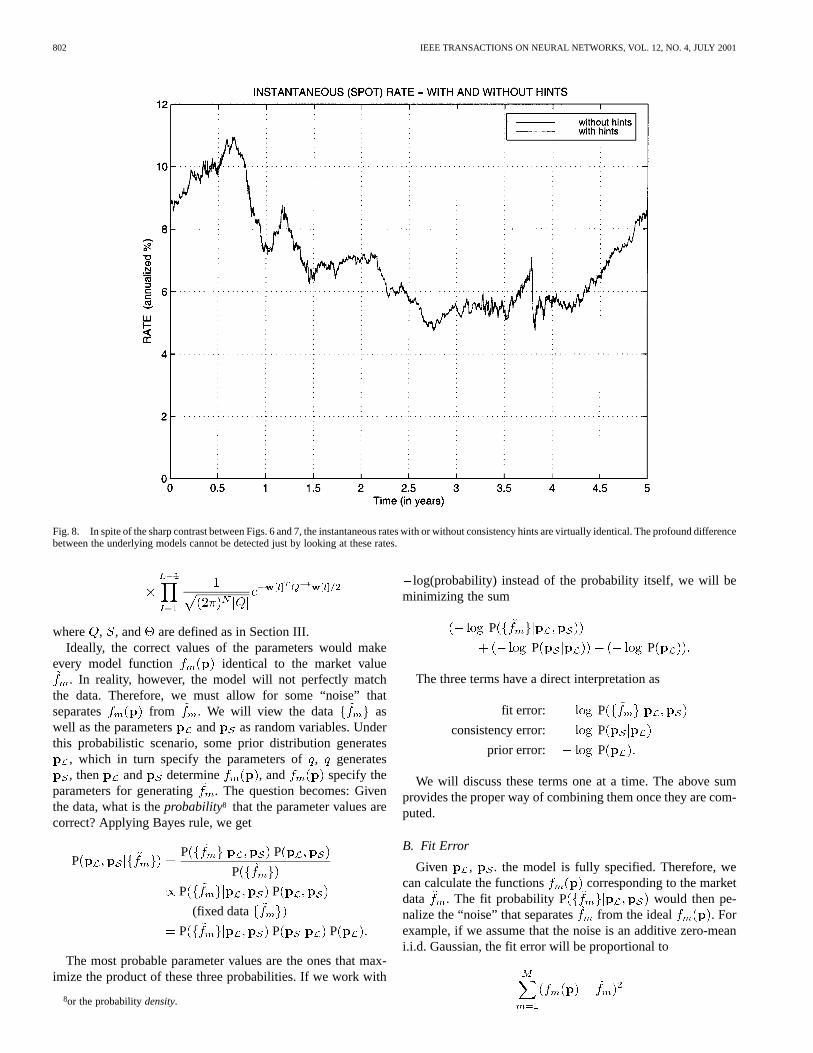
Fig. 8 shows the time evolution of the instantaneous rate forthe USD yield, with and without the hints. In spite of the twocalibrated models being quite different, the instantaneous ratesare similar, since they affect the value of the yield and we areusing the same yield data in both cases. The situation is analo-gous to Figs. 1 and 2, where just looking at the two fits wouldnot reveal the fundamental differences between the underlyingmodels, but these differences result in vastly different volatilityterm structures.

Finally, we show the impact of enforcing consistency hintson the quality of the fit. It is conceivable that the hints maysignificantly constrain the fitting of the data, and a much worse

6The onset of the Asian crisis in 1997 inflated the short-term rates by whatwas called the “Japan premium.”


Fig. 6. Time evolution of the state variables in a 3-factor Vasicek model calibrated to USD yield data with consistency hints. The ‘bubbles’ show the3� rangewithin which the evolution should take place.

fit error would result. However, as we see in Fig. 9, the impactis negligible in this case.

V. STATISTICAL INTERPRETATION

In this section, we put calibration in a statistical framework.This will provide a more principled way of making certain

choices that would otherwise be made in a heuristic way. Inparticular,

1) it will provide a rationale for the relative weight betweenthe fit error and the hint errors in the objective function;

2) it will enable us to bring other consistency hints, as wellas a prior condition, into the picture;

3) it will provide a methodology for standardizing the dif-ferent error measures, i.e., converting them to the same“units.”


Fig. 7. Time evolution of the state variables in a 3-factor Vasicek model calibrated to USD yield data without consistency hints. The “bubbles” show the3� rangewithin which the evolution should have taken place, but did not.

A. Probabilistic Setting

The premise of calibration is that the Vasicek model would bevalid if the parameters (long-term , and short-term ) wereproperly chosen. Validity of the model means that the pdf forgenerating has the form specified by the model, with

determining the parameters of this pdf. The statevariables ; , , which are theshort-term parameters , aregeneratedby the pdf. We obtaina simpler version of the pdf if we represent by the initial

state and the stochastic elements ; .This pdf7 is given by

7We useq to denote the joint pdf, and also to denote its marginal componentsas in Section III.


Fig. 8. In spite of the sharp contrast between Figs. 6 and 7, the instantaneous rates with or without consistency hints are virtually identical. The profound differencebetween the underlying models cannot be detected just by looking at these rates.

where , , and are defined as in Section III.Ideally, the correct values of the parameters would make

every model function identical to the market value. In reality, however, the model will not perfectly match

the data. Therefore, we must allow for some “noise” thatseparates from . We will view the data aswell as the parameters and as random variables. Underthis probabilistic scenario, some prior distribution generates

, which in turn specify the parameters of, generates, then and determine , and specify the

parameters for generating . The question becomes: Giventhe data, what is theprobability8 that the parameter values arecorrect? Applying Bayes rule, we get

PP P

P

P P

(fixed data

P P P

The most probable parameter values are the ones that max-imize the product of these three probabilities. If we work with

8or the probabilitydensity.

log(probability) instead of the probability itself, we will beminimizing the sum

P

P P

The three terms have a direct interpretation as

fit error: P

consistency error: P

prior error: P

We will discuss these terms one at a time. The above sumprovides the proper way of combining them once they are com-puted.

B. Fit Error

Given , . the model is fully specified. Therefore, wecan calculate the functions corresponding to the marketdata . The fit probability P would then pe-nalize the “noise” that separates from the ideal . Forexample, if we assume that the noise is an additive zero-meani.i.d. Gaussian, the fit error will be proportional to


Fig. 9. The daily root mean square error in fitting the USD yield data, with and without consistency hints. With the hints constraining the fit, there isonly anegligible increase in the fit error.

which is the expression for in Section II. The constant of pro-portionality is inversely related to the variance of the Gaussian.Thus, the relative weight between the fit error and the hint errorscan be derived from assumptions about the noise level.

C. Consistency Error

The long-term parameters affect the consistency error di-rectly by modifying , , and in the expression of , andindirectly when we solve for the implied by substitutingthe state variables into the difference equations. The consistencyerror P fixes in the expression of, and eval-uates . Substituting the expression of, this re-duces to the initial-state error plus the cross entropy part of

. Therefore, even without imposing hintsper se, the Bayesianequation almost recreates the errorsand of Section III.

Hints come into play because of overfitting. In order to op-timize the objective function, we pursue many combinationsof and , based on a finite set of data. In doing so, wemay introduce anomalies in the solution that would be very rareif we considered only one combination of the parameters. Toavoid such anomalies, the search needs to be regularized or con-strained. Hints provide constraints based on the properties of themodel. As such, they do not exclude good solutions.

For instance, the entropy part of the hint errorpulls ;away from the solution . This solution

is the single most “probable” solution for , since assumesits maximum value there. The solution is nonetheless undesir-able, since a typical solution for would have a variety ofvalues that reflect the Gaussian distribution (the goodness of fit[10] seen in Fig. 5, but not in Fig. 4). If we generate a singlesolution, it is likely to be of the typical variety. However, if weactively seek a high-probability solution, we will get one, and itmay be atypical. The contrast between “probable” and “typical”comes up in many contexts, most notably in information theory[4].

We will introduce other hint errors that also constrain the so-lution in a meaningful way. In deriving , we made certainassumptions that we can exploit now to create the new hints.For instance, the Kullback-Leibler distance should havebeen based on the full joint, a situation we avoided because itwould have rendered the entire , a one-point sample, withno hope of creating a meaningful estimate. Working with themarginal solved this problem, but left certain properties of thejoint untested. One such property is that should be statis-tically independent for different. We will create a correlationerror function that penalizes statistical dependence. Also, theentropy part of was based on a Gaussian assumption about, and we will create hint errors that penalize violations of this

assumption. Finally, the entropy estimate was not sensitive tothe mean of the distribution, and we will create a bias errorthat penalizes if it has a nonzero mean. Here are the details.


1) Bias: The form of asserts that ; ,have zero mean. If so, must also have zero mean for anyconstant . Let9

Based on and , we can define the bias error function

which measures the normalized bias ofalong the worst-caseprojection. The expression can be reduced to

which is a simple function of the implied .2) Correlation: asserts that is uncorrelated with, among other things. If so, must also be uncorrelated

with for any constant . Let

Based on and , we can define the correlation error func-tion

which measures the normalized covariance, again along theworst-case projection. The expression can be reduced to themaximum absolute eigenvalue of , where

with and being the eigenvalue matrix and eigenvector ma-trix of ( and ).

3) Gaussianity: asserts that are normally distributed.If so, the higher order moments around the mean should be re-lated to the variance accordingly. For instance, the third momentthat measuresskewnessshould be zero, and the fourth momentthat measureskurtosis10 should be three times the square of thevariance. One can define error functions and based ondeviations from these values.

Together with and , the new error measures , ,, and capture many aspects of the pdf. The list is by no

means exhaustive. It is inevitable for a finite sample realizationof a pdf to have anomalies along some dimension. What we havedone here was to develop consistency hints that penalize a fewobvious anomalies that may arise with overfitting.

9For an unbiased version of�, a normalizing factor of1=(L� 2) instead of1=(L� 1) would be used.

10Kurtosis quantifies “fatness of the tail,” which is among the more vulnerableaspects of the Gaussian assumption in models like the Vasicek.

D. Prior Error

P assigns a prior probability to the long-term parameters. There are reasons for preferring one set

of parameters over the other in the absence of any data. Someof the reasons are the following.

1) Hard constraints arising from the model assumptions suchas , , and being positive definite.

2) Economic considerations such as plausible values for theequilibrium interest rate .

3) Moving window calibration that allows long-term param-eters to change slowly from one window to the next. Inthis case, the solution for in the old window becomesthe center of a concentrated prior distribution for the newwindow.

E. Canonical Errors

The consistency error functions that we derived have differentscales. Some are based on pdfs, others on measures such as en-tropy, and others on various heuristics. Even the premise of anerror function can vary. For instance, the bias error could havebeen based on a fixed projection instead of the worst-case pro-jection. Therefore, the values of these error functions, in the ab-solute, do not mean much. In order to combine the errors in ameaningful way, we would like to convert them to a uniformscale. This can be done using probability as a common ground.

Let be an error function. We only require that betruly an error function, i.e., one for which larger values ofcorrespond to worse values of. If is stochastic, becomesa random variable. In this case, we define the canonical version

of as follows:

Pr

In other words, the value of for a given is based on thetotal probability of all sets of parameters for which the value of

is no better than . One can view this as a natural groupingof the parameters induced by.

The definition implies that is actually . Insome cases, it is possible to find an analytic formula for .In other cases, can be evaluated based on numericalintegration. If all else fails, it is possible to estimate usingMonte Carlo simulations. To do this, generate the long-termparameters according to the prior (or fix them at a typicalvalue), and generate according to , then compute andhistogram it. can now be estimated from the histogramthrough curve fitting. The accuracy of the fit is more importantfor smaller values of since the real tradeoff between differenterrors does not take place until they are relatively small.Fortunately, that’s where more points fall in the histogram,allowing for a better fit.

In general, will be different for different (number ofVasicek factors), and will also vary with the calibration windowsize, sometimes in a predictable way. Fig. 10 illustrates theMonte Carlo procedure for the consistency error function.We use the number of factors and the calibration window sizeof the JPY swaps experiment.

Regardless of the range of values for, the canonical willbe greater than or equal to zero, with equality whenachieves


(a)

(b)

(c)

Fig. 10. Generating the canonical error version ofE for the 3-factor Vasicek. (a) Histogram of consistency hint error E1. A Monte Carlo simulation uses themodel to generate a histogram of the values ofE . (b) Implied probability that E1 exceeds a certain level. The histogram is used to infer the probability thatE

exceeds a certain level, and an analytic formula is fit to that probability. (c) Canonical error function for E1. Taking� log of the formula, we get the value of thecanonical error for any value ofE .

its minimum possible value. The value ofhas a uniform in-terpretation. For instance, always corresponds to a prob-ability of or 0.37%.

If we have a number of statistically independent errors, theirs can be combined by simple addition. Even with errors that

are not quite statistically independent, our experience is that

adding the canonical errors still works in practice.11 This al-lows us to mix all types of error measures in the same objectivefunction.

11Alternatively, one could define a joint version ofE when the errors arenot statistically independent. The Monte Carlo estimate in this case requires farmore simulations.


VI. CONCLUSION

Calibration of financial models must conform to the assump-tions of these models. If calibration is based only on fitting thedata, it is liable to violate these assumptions. To guarantee thatthis does not happen, consistency hints are introduced as con-straints on the calibration process. The Kullback-Leibler dis-tance quantifies the main constraint. To balance the hint errorfunctions, canonical errors are introduced. Consistency hintscan be implemented with an efficient optimization algorithm.They are successfully applied to calibrating the correlated mul-tifactor Vasicek model of interest rates in the JPY swaps marketand the USD yield market.

APPENDIX I

In this Appendix, we provide the definitions and derivationsof the correlated multi-factor Vasicek model. The reader maywish to get a more detailed account of interest-rate models [14],SDEs [15], and Ito calculus [13].

The Vasicek -factor model for interest rates is given by thefollowing set of SDEs:

where , , and are constants, and areWiener processes whose covariances are given by

where

The instantaneous interest rateis given by

A. The Discount Function

The discount function computes the value, at thepresent time, of “a future dollar” at time

which can also be interpreted as the price of a unit bond of ma-turity . The following expression solves for underthe Vasicek model

To prove this, we use the fact that , andintegrate the SDEs to obtain

for . Therefore

where the last term resulted from integration by parts. Let uscall this last term

is a zero-mean Gaussian with variance

var

since , andfor by the

properties of the Wiener processes. In terms of, since, we can write

but for a zero-mean Gaussian . Substi-tuting


Carrying out the integration results in the required expression.

B. Other Market Functions

Many model-based market functions follow from the dis-count function. For example, the yield functionestimates the interest rate between timesand , expectedat time

The forward rate function is the instantaneous rateat time expected at time

The swap par rate is the fixed interest rate that can be evenlyexchanged for a floating rate. It assumes that we are receivingat times , the return on one dollarinvested earlier at the prevailing interest rate at the time ofinvestment. In return, we must pay out at the same times ,

constant payments of each, which canbe thought of as simple interest on one dollar investedearlierat rate . The par rate is the value of that would make thesetwo cash flows equitable. It is denoted by , andis given by

For all of these functions, we can obtain a Vasicek formulaby substituting the formula for . For instance

The only state variables appearing in these formulas are the“current states,” i.e., the state variables at the presenttime (the time when the quantities are measured). This factsimplifies the logistics of fitting market functions to market data.

The final market function used in this paper is the volatilityterm structure (VTS) of the forward rate. Given the Vasicek for-mula for , if we hold constant, we can write

Substituting from the Vasicek SDEs, the stochastic part ofis given by . Therefore, the variance ofis given by

var

The VTS is defined by var . There-fore,

which is constant with regard toand does not depend on statevariables. In Fig. 2, the theoretical VTS was computed by thisformula, while the historical VTS was based on the sample stan-dard deviation of changes in from day to day.

C. Discrete-Time Approximation

To derive a discrete-time version of the Vasicek model, weconsider one step in time fromto , and integrate theSDEs to get

Rewriting as and rearranging, weget

which can be rewritten as

The last term follows from the properties of Wiener pro-cesses, with being jointly Gaussian with zero mean anda covariance given by

Furthermore, are independent for different times withnonoverlapping . This expression for is the exact dif-ference equation for the Vasicek model. If , we canapproximate it by a difference equation similar to the SDE.

where , , and . Whendiscrete time is used, we adopt the usual notation of bracketedindex arguments. Thus, time will be denoted by, and thecorresponding and will be and .

ACKNOWLEDGMENT

The author would like to acknowledge Dr. M. Magdon-Is-mail for his useful hints and to thank the members of Caltech’sLearning Systems Group for helpful discussions.

REFERENCES

[1] Y. Abu-Mostafa, “Learning from hints in neural networks,”J. Com-plexity, vol. 5, pp. 192–198, June 1990.


[2] , “Machines that learn from hints,”Sci. Amer., vol. 272, no. 4, pp.64–69, Apr. 1995.

[3] , “Hints,” Neural Comput., vol. 7, pp. 639–671, July 1995.[4] T. Cover and J. Thomas,Elements of Information Theory: Wiley, 1991.[5] A. Dempsteret al., “Maximum likelihood for incomplete data via the

EM algorithm,”J. Roy. Statist. Soc., vol. B39, pp. 1–38, Jan. 1977.[6] W. Feller, An Introduction to Probability Theory and Its Applica-

tions. New York: Wiley, 1968, vol. 1.[7] R. Fletcher and C. Reeves, “Function minimization by conjugate gradi-

ents,”Comput. J., vol. 7, pp. 149–154.[8] R. Horn and C. Johnson,Matrix Analysis. Cambridge, U.K.: Cam-

bridge Univ. Press, 1985.[9] S. Kullback and R. Leibler, “On information and sufficiency,”Ann.

Math. Statist., vol. 22, pp. 79–86, 1951.[10] R. Larsen and M. Marx,An Introduction to Mathematical Statistics and

Its Applications. Englewood Cliffs, NJ: Prentice-Hall, 1986.[11] R. Lupton,Statistics in Theory and Practice. Princeton, NJ: Princeton

Univ. Press, 1993.[12] J. Moody, “The effective number of parameters: An analysis of gener-

alization and regularization in nonlinear learning systems,” inAdvancesin Neural Information Processing Systems, J. Moody, S. Hanson, and R.Lippmann, Eds. San Mateo, CA: Morgan Kaufmann, 1992, vol. 4, pp.847–854.

[13] S. Neftci, An Introduction to the Mathematics of Financial Deriva-tives. New York: Academic, 1996.

[14] R. Rebonato,Interest-Rate Option Models. New York: Wiley, 1996.[15] Z. Schuss,Theory and Applications of Stochastic Differential Equa-

tions. New York: Wiley, 1980.[16] J. Shore and R. Johnson, “Axiomatic derivation of the principle of

maximum entropy and the principle of minimum cross-entropy,”IEEETrans. Inform. Theory, vol. 26, pp. 26–37, Jan. 1980.

[17] B. Silverman, Density Estimation for Statistics and Data Anal-ysis. London, U.K.: Chapman and Hall, 1993.

[18] O. Vasicek, “An equilibrium characterization of term structure,”J. Fi-nancial Economics, vol. 5, pp. 177–188, Nov. 1977.

[19] P. Wilmott et al., The Mathematics of Financial Deriva-tives. Cambridge, U.K.: Cambridge Univ. Press, 1995.

Yaser S. Abu-Mostafa received the B.Sc. degreefrom Cairo University, Cairo, Egypt, in 1979, theM.S.E.E. degree from the Georgia Institute ofTechnology, Atlanta, in 1981, and the Ph.D. degreefrom California Institute of Technology (Caltech),Pasadena, in 1983.

He is Professor of Electrical Engineering andComputer Science, and Head of the LearningSystems Group, at the California Institute ofTechnology. His research interests include machinelearning, computational finance, and neural net-

works, and he has more than 80 technical publications including two articles inScientific American.

Dr. Abu-Mostafa was a founding member of the IEEE Neural NetworksCouncil, and the founding program chairman of the Neural InformationProcessing Systems (NIPS) Conference. He chaired a number of nationaland international conferences, most recently the international conference onComputational Finance(CF’99), and has served on the boards of ten journals.Since 1988, he has been a technical consultant for a number of financial firms,including Citibank for nine years. Among his awards are the 1996 Richard P.Feynman Prize for excellence in teaching, and the 1998 Kuwait State Awardin Applied Science. He was awarded the Clauser Prize for the most originaldoctoral thesis.

financial model calibration using consistency hints...

Documents