Financial Markets, Monetary Policy

and Reference Rates:

Assessments in DSGE Framework

Nao Sudo * nao.sudou@boj.or.jp

No.12-E-12 December 2012

Bank of Japan 2-1-1 Nihonbashi-Hongokucho, Chuo-ku, Tokyo 103-0021, Japan

* Financial System and Bank Examination Department

Papers in the Bank of Japan Working Paper Series are circulated in order to stimulate discussion

and comments. Views expressed are those of authors and do not necessarily reflect those of

the Bank.

If you have any comment or question on the working paper series, please contact each author.

When making a copy or reproduction of the content for commercial purposes, please contact the

Public Relations Department (post.prd8@boj.or.jp) at the Bank in advance to request

permission. When making a copy or reproduction, the source, Bank of Japan Working Paper

Series, should explicitly be credited.

Bank of Japan Working Paper Series

Financial Markets, Monetary Policy and Reference Rates:Assessments in DSGE Framework�

Nao Sudo

December 28, 2012

Abstract

In this paper, we explore the roles played by reference rates in business cycle �uctuationsusing a medium-scale full-�edged dynamic stochastic general equilibrium (DSGE) model. Ourmodel is an extended model of chained-credit-contract model developed by Hirakata, Sudo,and Ueda (2011b) estimated by the Japanese data. In our economy, there are interbank aswell as lending markets. Credit spreads determined in the markets are a¤ected by the borrow-ers�creditworthiness and degree of informational friction in the credit markets. Focusing onthe role of reference rates that a¤ects economic decisions through the delivery of informationabout the nature of economy, we evaluate channels through which the reference rates a¤ectscredit spreads and macroeconomic activities. We �nd that (i) reference rates may mitigateinformational friction in the credit markets, leading to a higher investment, output, and in-�ation, (ii) reference rates may contribute to economic stabilization by providing accurateeconomic forecast, and (iii) reference rates may bring about unintended consequence of mon-etary policy implementation by adding a noise to the credit spreads. Our results indicate theimportance of reliable reference rates, particularly under the environment where uncertaintyprevails, from the perspective of resource allocation, stabilization, and policy implementation.

Keywords: Reference Rates; Credit Spreads; Informational Friction, Signal Extraction, Mone-tary Policy

�Director, International Division, Financial System and Bank Examination Department, Bank of Japan (E-mail:nao.sudou@boj.or.jp). The author would like to thank Kosuke Aoki, Ichiro Fukunaga, Jacob Gyntelberg, DaisukeIkeda, Selahattin Imrohoroglu, Sohei Kaihatsu, Koichiro Kamada, Ryo Kato, Tomiyuki Kitamura, Shun Kobayashi,Marco Lombardi, Koji Nakamura, Kenji Nishizaki, Yukisato Ohta, Masashi Saito, Yuki Teranishi, Yuki Uchida,Yoichi Ueno, and Hiromi Yamaoka for their useful comments. Views expressed in this paper are those of the authorand do not necessarily re�ect the o¢ cial views of the Bank of Japan.

1

1 Introduction

Since the �nancial crisis starting in 2007, a growing attention has been paid to the role played by thereference rates in �nancial transactions among both policy makers and scholars. Although there is astrong agreement about the usefulness of the reference rate in guiding pricing of �nancial products,some recent studies emphasize a negative side of a coin. For instance, Abrantez-Mtez et. al (2012),investigating empirically if manipulations have been in place particularly during the �nancial crisis,suggest that Libor rates may have su¤ered, though not materially, from manipulation problem.1

In this paper, we ask roles of reference rates in business cycle �uctuations.2 To this end, wemake use of a medium-scale full-�edged dynamic stochastic general equilibrium (DSGE) modeldeveloped by Muto, Sudo, and Yoneyama (2012, hereafter MSY)3 and discuss how reference ratea¤ects economic behavior of agents, credit spreads in �nancial transaction, and macroeconomicperformance. Our model is built upon a chained-credit-contract model developed by Hirakata,Sudo, and Ueda (2009, 2011a, b, hereafter HSU) and is estimated using Japanese data from the1980s to 2000s. In our economy, there are credit constrained �nancial intermediaries (hereafterFIs) as well as credit constrained goods producing �rms and those borrowing sectors raise externalfunds from the interbank market and lending market, respectively. Similarly to Bernanke, Gertler,and Gilchrist (1999), there is informational friction between lenders and borrowers. That is, whileborrowers�output are diverse, lenders cannot observe realization of each borrower�s output unlessmonitoring is conducted. When lenders recognize that either borrowers� riskiness or expenseassociated with monitoring goes up, then lenders charge higher spread on their lending rates.While credit spreads are primarily a¤ected by the borrowers�creditworthiness measured by sizeof net worth, degree of informational friction in credit markets also plays the important role indetermining the spreads.We study three distinct channels through which reference rate a¤ects macroeconomy. The

�rst channel stresses in�uence of reference rate on informational friction in the credit markets.We consider a case where a reliable reference rate reduces cost of monitoring activities associatedwith �nancial intermediation and a case where it reduces borrowers�diversity regarding perceivedidiosyncratic productivity from lenders�perspective. When monitoring cost is less costly, expecteddefault cost falls and credit spread tightens, facilitating �nancial intermediation and boostingthe economy. Similarly, when lenders perceive that idiosyncratic productivity converges acrossborrowers, because expected portion of defaulting borrowers falls, credit spreads shrink, givingway to economic expansion.The second channel stresses in�uence of reference rates on agents�forecast and its implication

for macroeconomic stability. We consider a case where agents today receive news about future eco-nomic events. While agents decide the current economic activities taking the information containedin the news into their consideration, the news is contaminated with noises and agents�expectationof the future events conditional on the news may depart from what will actually materialize. Thediscrepancy between the today�s forecast and realization of the future events yields an additionalsource of business cycle �uctuations. When reference rates deliver accurate information about thefuture economic events, the discrepancy shrinks, achieving economic stability.

1By contrast, Kuo, Skeie, and Vickery (2012) discuss that Libor rates generally comove with other measures ofborrowing rates although they �nd that Libor quotes sometimes lie below these measures and less disperse comparedto them. See also Snider and Youle (2010) for related discussion.

2In contrast to our study that focuses on the role of reference rates in the macroeonomic activity, Muto (2012)studies the role in the interbank interest rates.

3See also Kawata et al. (2012) for the evaluation of role of reference rates in the macroeconomic �uctuationsusing a �nancial macro-econometric model.

2

The third channel stresses in�uence of reference rates through a monetary policy implementa-tion. We consider a case where a monetary authority cannot observe a noise in the credit spreadsseparately from the fundamental variations. While the noise itself is a non-fundamental innova-tion, when a policy rate systematically responds to credit spreads that contains the noise, the noisecauses an unintended consequence from the central bank�s perspective. From the private agents�perspective, the response of the policy rate acts as a shock to the monetary policy rule, adverselya¤ecting macroeconomic stability.This paper is organized into six sections. Section 2 brie�y describes our model. The model

consists of two categories of �nancial markets, interbank market and lending markets, and threetypes of market participants, investors, FIs, and entrepreneurs. Credit spreads in the modelare determined by two factors: creditworthiness of borrowers and degree of informational frictionbetween borrowers and lenders. Here, reference rate a¤ects both two factors. In section 3, 4, and 5,we propose three channels through which reference rate a¤ects credit spreads and macroeconomicactivities by providing agents information regarding the nature of the economy. Section 3 discussesthe role of reference rate in reducing degree of informational friction in credit markets. When thefriction is mitigated, credit spreads shrink and aggregate investment becomes less costly. Section 4discusses the role of reference rate in helping agents�expectation formation about future economicevents and stabilizing business cycle �uctuations. Section 5 explores the case when reference ratecontains non-fundamental noises and a¤ects monetary policy implementation. Section 6 draws aconclusion.

2 The economy

This section describes our model structure. The model is borrowed from MSY (2012) and themodel outline is shown in Figure 1. The economy consists of �ve sectors: the household sector, the�nancial intermediary (FI) sector, the non-durables sector, the durables sector, and the governmentsector. The household sector consists of two agents, the representative household and the investors.The representative household supplies labor inputs to the goods-producing sectors, earns wage,makes a deposit to the investors, and receives repayment in return. The investors collect depositsfrom the household and lend them to the FI sector by making credit contracts called IF contractswith the FIs. The FIs raise the external funds from the investor through the IF contracts andlend them to the goods-producing sectors by making credit contracts with each of the sectors. Wecall each of the contracts, the FEC and the FED contract, respectively. Each goods-producingsector consists of three agents, the entrepreneurs, the capital goods producers, and the goodsproducers. The entrepreneurs raise external funds from the FIs, purchase capital goods from thecapital goods producers using the funds, and provide the capital goods to the goods producers.They then earn the rental price of the capital goods in return, accumulating the earnings as thenet worth. The capital goods producers purchase investment goods from the durables sector andproduce the capital goods. The goods producers produce goods from labor input, capital goods,and intermediate goods. Government sector consists of the government and the central bank. Thegovernment collects tax from the household sector and spends the tax revenue for the governmentpurchase. The central bank adjusts the nominal interest rate so as to stabilize the in�ation rate.

3

2.1 Credit Contracts

2.1.1 FEC and FED Contracts

Basic SettingThe FEC and FED contract are made between a FI and a continuum of the entrepreneurs in the

two goods-producing sectors. In period t; each type i FI o¤ers a loan contract to an in�nite numberof group ji� entrepreneurs in sector �. An entrepreneur in group ji� owns net worth N�;ji�

(st) andpurchases capital of Q� (s

t)Kji�(st), where st is the whole history of states until period t, Q� (s

t)

is the price paid per unit of capital and Kji�(st) is the quantity of capital purchased by the group

ji� entrepreneur in sector �: Since the net worth N�;ji�(st) of the entrepreneur is smaller than

the amount of the capital purchase Q� (st)Kji�

(st) ; the entrepreneur raises the rest of the fundsQ� (s

t)Kji�(st) � N�;ji�

(st) from the type i FI.The net return to a capital of a group ji� entrepreneur is a product of the two elements: an

aggregate return to capitalR� (st+1) in sector � and an idiosyncratic productivity shock !�;ji� (s

t+1) ;

that is speci�c to the group ji� entrepreneur.4 There is informational asymmetry between lenders

and borrowers and the FI cannot observe the realization of the idiosyncratic shock !�;ji� (st+1)

without paying the monitoring cost ��: Under this informational friction, the FEC and FEDcontracts specify:

� amount of debt that the group ji� entrepreneur borrows from a type i FI, Q� (st)Kji�

(st) �N�;ji�

(st) ; and

� cut-o¤value of idiosyncratic productivity shock !�;ji� (st+1) ;which we denote by !�;ji� (s

t+1) ;

such that the group ji� entrepreneur repays its debt if !�;ji� (st+1) � !�;ji�

(st+1) and declaresthe default if otherwise.

Entrepreneurs�participation constraintA group ji� entrepreneur joins the FEC or FED contract only when the return from the credit

contract is at least equal to the opportunity cost. Based on the FEC or FED contract, a portionof the entrepreneurs

R1!�;ji�

(st+1)dF� (!�) does not default and the rest of them default. If they do

not default, ex post, they receive the net return to its capital holdings:�!�;ji�

�st+1

�� !�;ji�

�st+1

��R�

�st+1

�Q�

�st�Kji�

�st�:

The entrepreneurial loan rate in sector � is therefore given by

r�;ji�

�st+1

��!�;ji�

(st+1)R� (st+1)Q� (s

t)Kji�(st)

Q� (st)Kji�(st)�N�;ji�

(st): (1)

4Here, !�;ji� (st) is a unit mean, lognormal random variable distributed independently over time and across

entrepreneurs in sector �. We express its density function by f��!�;ji�

�; and its cumulative distribution function

by F��!�;ji�

�:

4

Instead of participating in the FEC or FED contract, a group ji� entrepreneur can purchase capitalgoods using only its own net worth N�;ji�

(st) : In this case, ex ante, the entrepreneur expects to re-

ceive the earningR� (st+1)N�;ji�

(st) ; and ex post it receives the earning !�;ji� (st+1)R� (s

t+1)N�;ji�(st).

Therefore, the FEC and FED contract between a type i FI and group ji� entrepreneur is agreedby the group ji� entrepreneur only when the following inequality is expected to hold:

R�

�st+1

�Q�

�st�Kji�

�st�0@Z 1

!�;ji�(st+1jst)

�!� � !�;ji�

�st+1jst

��dF� (!�)

1A � R�

�st+1

�N�;ji�

�st�for 8ji� :

(2)

FIs�pro�t from the credit contracts with the goods-producing sectorsBased on equation (2), the expected earnings of the type i bank from the FEC and FED

contracts are given byX�=c;x

Zji�

��i�st+1jst

�R�

�st+1jst

�Q�

�st�Kji�

�st�dji� ;

where

��i�st+1jst

��Z 1

!�;ji�(st+1jst)

!�;ji�

�st+1jst

�dF� (!�)� ��

Z !�;ji�

0

!�dF� (!�) ; for � = c; x: (3)

Note that term associated with �� accounts for the ex post monitoring cost that a type i FI payswhen a group ji� entrepreneur in the � sector declares the default.The type i FI makes a contract with a in�nite number of group ji� entrepreneurs in sector �,

and as shown in HSU (2009), the cut-o¤ value !�;ji� that is chosen by the type i FI is identicalacross all entrepreneurs in sector � that make contract with the type i FI: Consequently, the FI�sexpected total return from both the FEC and FED contracts is given byX

�=c;x

��i�st+1jst

�R�

�st+1jst

�Q�

�st�Ki�

�st�;

where

Ki�

�st��Zji�

Kji�

�st�dji� ; for � = c; x:

For the convenience of analysis below, we de�ne the total amount of net worth held by the groupji� entrepreneur in sector �.

N�;i

�st��Zji�

N�;ji�

�st�dji� ; for � = c; x:

2.1.2 IF Contracts

Basic setting

5

The IF contract is made between an investor and a continuum of the FIs. In period t; eachtype i FI holds the net worth NF;i (s

t) and makes loans to group ji� entrepreneurs in the sector �at an amount of Q� (s

t)K�;i (st)�N�;i (s

t) : Since the FI�s net worth is smaller than its loans to theentrepreneurs in the two sectors, it borrows the rest

P�=c;x [Q� (s

t)K�;i (st)�N�;i (s

t)] � NF;i (st)

from the investor. Similarly to the FEC and FED contracts, there is informational asymmetrybetween the lender and the borrowers. Each type i FI faces an idiosyncratic productivity shock!F;i (s

t+1) : This shock !F;i (st+1) represents technological di¤erences across the FIs, for example,those associated with risk management, maturity mismatch control, and loan securitization5. In-corporating this idiosyncratic shock, the FI�s receipt from the loans to the entrepreneurs is givenby6

!F;i�st+1

� "X�=c;x

��i�st+1jst

�R�

�st+1jst

�Q�

�st�Ki�

�st�#:

The investor can observe the realization of the shock only by paying the monitoring cost �F :Under this credit friction, the IF contract speci�es:

� amount of debt that a type i FI borrows from the investor,P

�=c;x [Q� (st)K�;i (s

t)�N�;i (st)]

� NF;i (st) ; and

� cut-o¤ value of idiosyncratic shock !F;i (st+1) ;which we denote by !F;i (st+1jst) ; such thatthe FI repays debt if !F;i (st+1) � !F;i (s

t+1jst) and declares the default if otherwise.

FIs�pro�t from the credit contractsAccording to the IF contract, a portion of the FIs

R1!F;i(st+1jst) dFF (!F ) do not default while the

rest of them default. The net pro�t of a non-default FI i equals its receipt from the FEC and theFED contract multiplied by the idiosyncratic shock !F;i (st+1) minus repayment to the investor:

�!F;i

�st+1

�� !F;i

�st+1jst

�� X�=c;x

��i�st+1jst

�R�

�st+1jst

�Q�

�st�Ki�

�st�!

:

The FIs�loan rate is therefore given by

rF�st+1jst

��!F;i (s

t+1jst)�P

�=c;x��i (st+1jst)R� (s

t+1jst)Q� (st)Ki� (s

t)�

P�=c;x [Q� (st)K�;i (st)�N�;i (st)]�NF;i (st)

:

Investors�participation constraintThere is a participation constraint for the investor in the IF contract. Given the risk-free rate

of return in the economy R (st) ; the investor�s pro�t from the investment in the loans to the banksmust at least equal to the opportunity cost of lending. That is

�F;i�st+1jst

� "X�=c;x

��i�st+1jst

�R�

�st+1jst

�Q�

�st�Ki�

�st�#

5See HSU (2010) for the alternative interpretations for !F;i (st) :6Similarly to the entrepreneurial riskiness !�;ji ; the FIs�riskiness !F;i is a unit mean, lognormal random variable

distributed independently over time and across FIs i. Its density function and its cumulative distribution functionare given by fF (!F;i) and FF (!F;i) ; respectively.

6

� R�st� "X

�=c;x

�Q�

�st�K�;i

�st��N�;i

�st���NF;i

�st�#

for 8i; st+1jst; (4)

where

�F;i�st+1jst

��Z 1

!F;i(st+1jst)!F;i

�st+1jst

�dFF (!F )� �F

Z !F;i(st+1jst)

0

!FdFF (!F ) : (5)

2.1.3 Optimal Credit Contract

Given the structure of the FEC, FED, and IF contract, a type i FI optimally chooses capital goodspurchased from capital goods producing sectors, the cut-o¤ value in the three classes of contracts,respectively. As shown in HSU (2009), since all FIs are identical in terms of ��i ;the expected pro�tof a type i FI is given by

�Z 1

!F (st+1jst)

�!F � !F

�st+1jst

��dFF (!F )

�"X�=c;x

���st+1jst

�R�

�st+1jst

�Q�

�st�Ki�

�st�#: (6)

The FI then maximizes the term (6), subject to the investor�s participation constraint (4) andentrepreneurial participation constraints (2).

2.1.4 Dynamic Behavior of Net Worth

The net worth of the FIs and the entrepreneurs in the two goods-producing sectors depend ontheir earnings from the credit contracts and their labor income. Both FIs and entrepreneursinelastically supply a unit of labor to goods producers in the goods-producing sectors and receivelabor income WFc (s

t) ; WEc (st) ; WFx (s

t) ; and WEx (st).7 The aggregate net worths of the FIs

and the entrepreneurs are given by

NF

�st+1

�= FVF

�st�+ "NF

�st�+X�=c;x

WF� (st)

PCPI (st); (7)

N�

�st+1

�= �V�

�st�+WE� (s

t)

PCPI (st)+ "N� for � = c; x; (8)

with

VF�st��

�Z 1

!F (st+1jst)

�!F � !F

�st+1jst

��dFF (!F )

�"X�=c;x

���st+1jst

�R�

�st+1

�Q�

�st�K�

�st�#;

V��st��

Z 1

!�(st+1jst)

�!� � !�

�st+1jst

��dF� (!�)

!R�

�st+1

�Q�

�st�K�

�st�; for � = c; x:

7See Bernanke, Gertler, and Gilchrist (1999), Christiano, Motto, Rostagno (2008) and HSU (2011a, b) for thetechnical background on introducing inelasitc labor supply from the FIs and the entrepreneurs.

7

Here, � for � = F; c; and x are probabilities that each FIs or entrepreneurs survive to the nextperiod. The FIs and the entrepreneurs who are in business in period t and fail to survive in periodt + 1 consume

�1� �

�V� (s

t) ; respectively. The net worth accumulations in the three sectorsare a¤ected by exogenous shocks represented by "N� (s

t) that is orthogonal to the fundamentalearnings from the credit contracts. We assume these shocks are i.i.d. They are �nancial shocksthat capture an �asset bubble,� �irrational exuberance,� or an �innovation in the e¢ ciency ofcredit contracts,�hitting the FI sector or the goods-producing sectors.

2.2 Households

Set upHousehold h is an in�nitely-lived representative agent with preference over the non-durables

consumption, C (h; st) ; service from the stock of durables, D (h; st) ; and work e¤ort, L� (h; st) for� = c; x, as described in the expected utility function, (9)

U0 � E0

1Xt=0

�t

264log �C c�h; st

�D d

�h; st

��� '

�P�=c;x L� (h; s

t)�1+v

1 + v

375 ; (9)

where � 2 (0; 1) is the discount factor, v > 0 is the inverse of the Frisch labor-supply elasticity, and' is the weighting assigned to leisure. The parameters � 2 (0; 1) for � = c; d represents relativeweights on utility from consuming each goods. The budget constraint for household h is given by

X�=c;x

P��st���h; st

�+ S

�i; st��

2664P

�=c;xW� (h; st)L� (h; s

t)

�P

�=c;x

�w�2

�W�(h;st)W�(h;st�1)

� 1�2

W� (st)L� (s

t)

+R (st�1)S (h; st�1) + (h; st) + � (h; st)

3775 ; (10)

where P� (st) denotes nominal prices of goods �, S (h; st�1) is the saving, Rs (st) is the nominal rate

on deposit, (h; st) is the nominal pro�t returned to the household, and � (st) is the lump-sumnominal transfer from the government. W� (h; s

t) is the nominal wage and W� (st) is aggregate

indices of the nominal wage in sector �. The second term in the right hand side of the equationstands for the nominal cost associated with adjusting nominal wageW� (h; s

t), and �w� is parameterthat governs the size of the cost.

Labor supply decisionHousehold h has the monopolistic power in its di¤erentiated labor input L� (h; st) in sector �.

The demand of the di¤erentiated labor is given by

L��h; st

�=

�W� (h; s

t)

W� (st)

���W�(st)L��st�for � = c; x; (11)

where L� (st) is aggregate indices of labor input in sector � that is de�ned as

L��st�=

�Z 1

0

L�;t�h; st

�(�W�(st)�1)=�W�(s

t)dh

��W�(st)=(�W�(s

t)�1)

for � = c; x;

8

where �Wc (st) and �Wx (s

t) 2 (1;1) deliver time-varying elasticity of labor demand for di¤erenti-ated labor input with respect to wages.

Durables accumulationThe law of motion for the stock of durables is given by

D�h; st

�= (1� �d)Dt�1

�h; st�1

�+

1� �dd

2

�Xt (h; s

t)

Xt�1 (h; st�1)� 1�2!

Xt

�h; st

�; (12)

where �d 2 (0; 1) is the depreciation rate of the durables stock, and �dd is the parameter associatedwith durable stock adjustment.

2.3 Goods Producers

Set upThe economy consists of two distinct sectors of production: the non-durables sector and

the durables sector. We assume that both sectors contain a continuum of �rms, each producingdi¤erentiated products, as indexed by l 2 [0; 1] and m 2 [0; 1] ; respectively. We use Cg (st) todenote a gross output of composite of di¤erentiated non-durables fCg (l; st)g l2[0;1], and Xg (s

t) todenote a gross output of composite of di¤erentiated durables fXg (m; s

t)g m2[0;1]: The productionfunctions of the two composites are

Cg�st�=

�Z 1

0

Cg�l; st�(�Pc(st)�1)=�Pc(st) dl��Pc(st)=(�Pc(st)�1) ;

Xg

�st�=

�Z 1

0

Xg

�m; st

�(�Px(st)�1)=�Px(st) dm��Px(st)=(�Px(st)�1) ;where �Pc (st) and �Px (s

t) 2 (1;1) denote the time-varying elasticity of substitution betweenproducts. The composite products are produced in an aggregation sector that faces perfect compe-tition. The demand functions for the non-durables �rm l and for the durables �rm m are derivedfrom the optimization behavior of the aggregation sector, represented by

Cg�l; st�=

�Pc (l; s

t)

Pc (st)

���Pc(st)Cg�st�and Xg

�m; st

�=

�Px (m; s

t)

Px (st)

���Px(st)Xg

�st�: (13)

These prices are related to the prices of the non-durables fPc (l; st)g l2[0;1] and the durablesfPx (m; st)g m2[0;1] by

Pc�st�=

�Z 1

0

Pc�l; st�(1��Pc(st)) dl�1=(1��Pc(st)) and Px �st� = �Z 1

0

Px�m; st

�(1��Px(st)) dm� :Resource constraintThe composites serve either as �nal goods and as intermediate production inputs. The alloca-

tion of the gross output of the non-durables is

9

Cg�st�= C

�st�+

Z 1

0

c�l; st�dl +

Z 1

0

x�m; st

�dm

+X�=c;x

���

Z !�

0

!�dF� (!�)

�R�

�st�Q�

�st�1

�K�

�st�1

�+�F

��F

Z !F

0

!FdFF (!F )

�(X�=c;x

���!��st��R�

�st�Q�

�st�1

�K�

�st�1

�)+X

�=c;x;F

�1� �

�V��st�; (14)

where fc (l; st)g l2[0;1] are intermediate production inputs used by �rm l in the non-durables sector,and fx (m; st)g m2[0;1] are intermediate production inputs used by �rm m in the durables sector.Note also that lenders in credit contracts consume non-durables in monitoring defaulting borrowers.The similar equation holds for a composite of durables Xg (s

t) and intermediate production inputsf�c (l; st)g l2[0;1], f�x (m; st)g m2[0;1]:

Xgt

�st�= X

�st�+

Z 1

0

�c�l; st�dl +

Z 1

0

�x�m; st

�dm+

X�=c;x

I��st�+Gx

�st�:

Production functionThe inputs used in each sector are labor, capital and intermediate inputs. The production

functions of the two goods-producing sectors are given by

Cg�l; st�=

264 Z (st)A (st)c (l; st) 11 �c (l; s

t) 21

[Lc (l; st)�]1� 11� 21h

[Kc (l; st)Uc (l; s

t)]1����E��FI

i1� 11� 21� Fc

375 ; (15)

Xg

�m; st

�=

264 Z (st)Zx (st)A (st)Ax (s

t)x (m; st) 12 �x (m; s

t) 22

[Lx (m; st)�]1� 12� 22h

[Kx (m; st)Ux (l; s

t)]1����E��FI

i1� 12� 22� Fx;

375 : (16)

Here, Z (st) and Zx (st) are the non-stationary component of technology that is common to thegoods-producing sectors and that is speci�c to the durables sector, respectively. Similarly, A (st)and Ax (st) are the stationary component of technology that is common to the goods producingsectors and that is speci�c to the durables sector, respectively. U� (st) and F� are the capacityutilization rate of capital input and �xed cost in sector �: The parameters ab for a; b = 1; 2 denotesthe cost share of total expenditure on inputs in sector a due to the purchase of intermediate inputsfrom sector b:

Price settingFirm l in the non-durables sector are monopolistic competitors in the products market where

they set prices for their products Pc (l; st) in reference to the demand given by (13) : It can resetthe prices solving the following problem:

10

maxfCg(l;st); Pc(l;st)gEt1Xq=0

�t+q�t

�c (l; st+q)

Pc (st+q); (17)

s:t: �c�l; st+q

�=

Pc (l; st+q)Cg (l; s

t+q)�MCc (l; st+q) (Cg (l; s

t+q) + Fc)

��pc2

�Pc(l;st+q)Pc(l;st+q�1)

� 1�2

Pc (st+q)Cg (s

t+q);

where �t+q is the Lagrange multiplier associated with budget constraint (10) ; and �pc is theparameter associated with non-durables price adjustment. The price setting of the durables sectorsis conducted in the similar way.

2.4 Capital Goods Producer

Capital goods producers in sector � for � = c; x convert investment goods I� (st) purchased fromdurables sector to capital goods K� (s

t), using technology FI� (st) ; and sell it to the entrepreneurs

in sector � with price Q� (st) : The capital goods producers�problem is to maximize the pro�t

function given below:

maxI�(st)

1Xq=0

��st+qjst

��t;t+q(s

t+q)

��Q�

�st+q

�K�

�st+q

�� (1� �)Q�

�st+q

�K�

�st+q�1

�� Px (s

t)

PCPI (st)I��st+q

��; (18)

where FI� is de�ned as follows:

FI��I��st+q

�; I��st+q�1

�; �I�

�st+q

����I� (s

t+q)

2

�I� (s

t+q)

I� (st+q�1)� 1�2

:

Note that �� (st+q) is a time-varying parameter that is associated with investment adjustment costin sector �.8 Because capital depreciates in each period, the evolvement of total capital used insector � available in period t is given by

K�

�st�=�1� FI�

�I��st�; I��st�1

���I��st�+ (1� �)K�

�st�1

�; (19)

where � 2 (0; 1) is the depreciation rate of the capital stock.

2.5 Aggregate Variables

Here, we de�ne some macroeconomic variables. The real GDP Yt (st) is de�ned as the weighted

average of value-added components:

Y�st���C�st���GDPc �X �st�+ Ic

�st�+ Ix

�st�+Gx

�st��1��GDPc ; (20)

where �GDPc is the steady-state expenditure share of the value-added produced by the non-durablessector. The GDP de�ator in�ation is given by

8See MSY (2012) for details of the capital goods producers�maximization problem.

11

��st�=�Pc�st�=Pc

�st�1

���GDPc �Px �st� =Px �st�1��1��GDPc :Using the in�ation rate de�ned above, the real interest rate is given by the Fischer equation thatconnects the nominal interest rate Rn (s

t) and the expected in�ation:

R�st�= Rn

�st�=Et�

�st+1jst

�:

2.6 Government Sector

The government collects a lump-sum tax � (st) from the household to �nance and governmentpurchase Px (st)Gx (s

t) whose amount is exogenously given:We assume that a balanced budget ismaintained in each period t as follows:

Px�st�Gx

�st�= �

�st�

The central bank adjusts policy rate according to the following Taylor rule:

logRn

�st�= �Rn

�st�1

�+ (1� �)' log �

�st�+ �Rn

�st�: (21)

Here, � 2 (0; 1) is the persistency parameter of monetary policy, ' > 1 is the policy weight attachedto the in�ation rate and �Rn (s

t) is an i.i.d. shock to the monetary policy rule.

2.7 Shock Process

The exogenous variables in our economy, the permanent technology in the two goods-producingsectors Z (st) ; the permanent technology in the durables sector Zx (st) ; the exogenous componentof the net worth in sector �; "N� (s

t) ; for � = F; c; or x; the government spending Gx (st) ; the

capital stock adjustment cost in sector �, �I� (st) ; the price markup in sector �; �P� (s

t) ; the wagemarkup in sector �; �W�

(st) ; and the technology of capacity utilization of capital inputs ZU (st)evolve according to the equation below:

lnZ�st�= lnZ

�st�1

�+ uZ

�st�; uZ

�st�= �ZuZ

�st�1

�+ �Z

�st�;

lnZx�st�= lnZx

�st�1

�+ uZx

�st�; uZx

�st�= �ZxuZx

�st�1

�+ �Zx

�st�;

"N��st�= �N�"N�

�st�1

�+ �N�

�st�; for � = F; c; x;

lnGx

�st�= (1� �Gx) lnGx + �Gx lnGx

�st�1

�+ �Gx

�st�;

ln�I ��st�= (1� �I �) ln�Ic + �I � ln�I �

�st�1

�+ �I �

�st�; for � = c; x;

ln �P �

�st�= (1� �P �

) ln �P �+ �P �

ln �P �

�st�1

�+ �P �

�st�; for � = c; x;

ln �W�

�st�= (1� �Wc

) ln �W�+ �W�

ln �W�

�st�1

�+ �W�

�st�; for � = c; x; and

lnZU�st�= (1� �U) lnZU + �U lnZU

�st�1

�+ �U

�st�;

where �Z ; �Zx ; �NF ; �Nc ; �Nx ; �Gx ; �Ic ; �Ix ; �Pc ; �Px ; �Wx, �Wc

and �U 2 (0; 1) are the autoregressiveroot of the corresponding shocks, and �Z (st) ; �Zx (s

t) ; �NF (st) ; �Nc (s

t) ; �Nx (st) ; �Gx (s

t) ; �Kc (st) ;

�Kx (st) ; �Pc (s

t) ; �Px (st) ; �Wc (s

t) ; �Wx (st) ; and �U (st) ; are the exogenous i.i.d. shocks that are

normally distributed with mean zero.

12

2.8 Equilibrium

An equilibrium consists of a set of prices, fPc (st) ; Px (st) ; Wc (st) ; Wx (s

t) ; Rc (st) ; Rx (s

t) ; R (st) ;Qc (s

t) ; Qx (st)g1t=0, and the allocations fC (st) ; Cg (st) ; Cg (l; st) ; c (l; st) ; x (m; st) ; X (st) ;

Xg (st) ; Xg (m; s

t) ; �c (l; st) ; �x (m; s

t) ; Ic (st) ; Ix (s

t) ; Lc (l; st) ; Lx (m; s

t) ; Kc (l; st) ; Kx (m; s

t) ;Uc (l; s

t) ; Ux (m; st) g1t=0; for all l;m 2 [0; 1] ; for given government policy fG (st) ; � (st) ; Rn (s

t)g1t=0,realization of exogenous variables f�Z (st) ; �Zx (st) ; �Rn (st) ; �A (st) ; �Ac (st) ; �NF (st) ; �Nc (st) ;�Nx (s

t) ; �Gx (st) ; �Kc (s

t) ; �Kx (st) ; �Pc (s

t) ; �Px (st) ; �Wc (s

t) ; �Wx (st) ; �U (s

t)g1t=0; and initial con-ditions fNF (s

�1)g; fNc (s�1)g; fNx (s

�1)g such that for all t ; the following conditions are satis�ed.(i) each household h maximizes his/her utility given the prices;(ii) each FI i maximizes its pro�ts given the prices and the net worths;(iii) each entrepreneurs jic and jix maximizes its pro�ts given the prices and the net worth;(iv) goods producer l in the non-durables sector and goods producer m in the durables sector

maximize their pro�ts given the prices;(v) capital goods producers in the two goods producing sectors maximize their pro�t given

prices;(vi) the government budget constraint holds;(vii) the central bank sets a policy rate following the Taylor rule; and(viii) markets clear.

3 Reference rate and informational friction

In this section, we investigate the relationship between informational friction in the credit marketsand the reference rates. To do this, we �rst discuss how credit spreads are determined. Assumingthat goods producing sectors are identical for simplicity so that Rc (s

t+1jst) = Rx (st+1jst) =

RE (st+1jst) holds, then equation (4) is arranged into the following form:9

RE (st+1jst)

R (st)=

P�=c;x [Q� (s

t)K� (st)�N� (s

t)]�NF (st)

�F (st+1jst)P

�=c;x�� (st+1jst)Q� (st)K� (st)

=1�

P�=c;xN�(st)P

�=c;xQ�(st)K�(st)

� NF (st)P�=c;xQ�(s

t)K�(st)

�F (st+1jst) �E (st+1jst); 8st+1jst:

RE (st+1jst) =R (st) captures credit spread between the rental cost of capital confronting goods

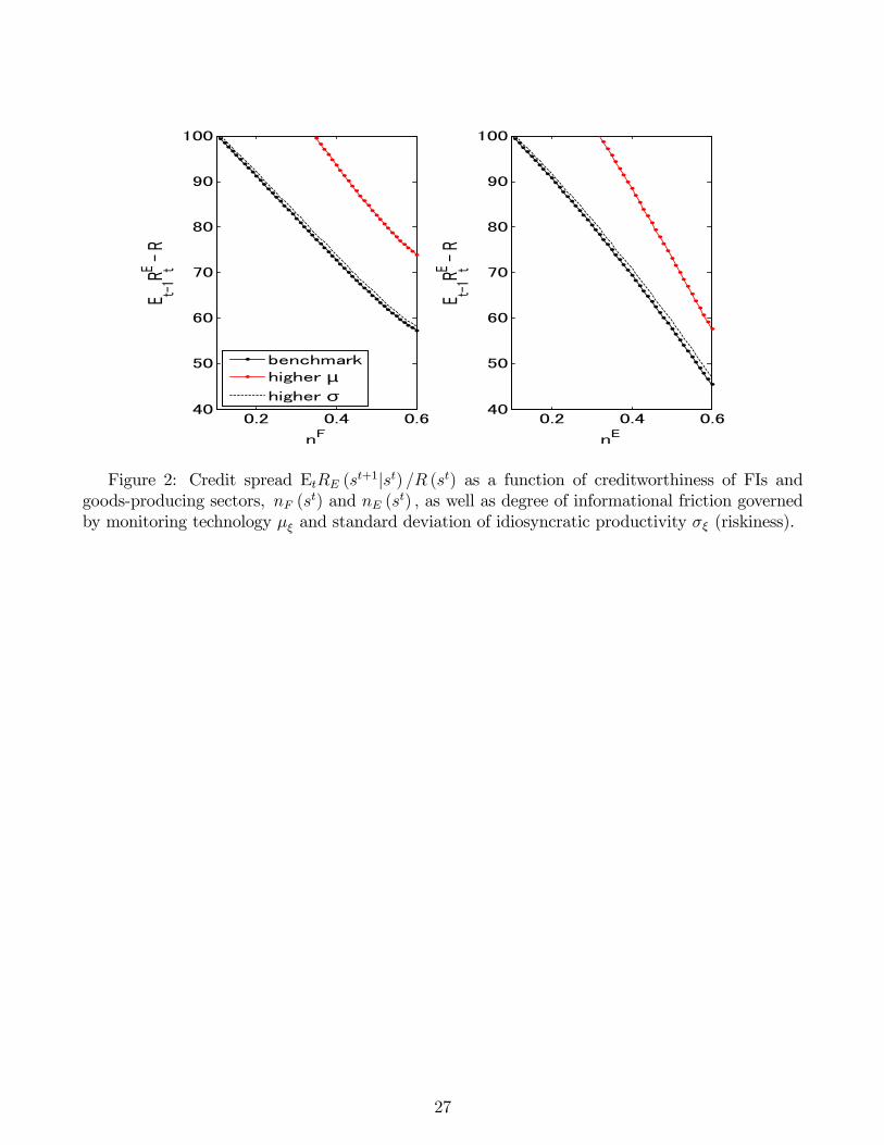
producing sectors and risk-free rate, and this credit spread is determined by the creditworthinessof borrowers as well as degree of informational friction. To see this, we demonstrate in Figure2 how the credit spread varies according to changes in the borrowers�net worth and the degreeof informational friction in credit markets. nF and nE denoted in the x-axis stand for the networth held by the FIs sector relative to total amount of investment and the net worth held by thegoods-producing sector relative to total amount of investment, respectively:

nF �NF (s

t)P�=c;xQ� (st)K� (st)

; and nE �P

�=c;xN� (st)P

�=c;xQ� (st)K� (st):

Clearly, the credit spread is negatively related to the creditworthiness of borrowers. Figure 3displays the working mechanism behind the relationship. As the net worth becomes more scarce

9Assuming that the two goods sector identical implies that ���st+1jst

�= �E

�st+1jst

�for � = c; x:

13

relative to the investment amount, the expected monitoring cost rises re�ecting a higher leverageand defaulting probability of borrowers. Because the lenders charge the expected monitoring costson their lending rates to the borrowers, the credit spreads widen.Creditworthiness is not the only determinant of the credit spread in the model. To see this,

we depict how the credit spread is altered when degree of informational friction is enhanced. Weconsider two cases: a deterioration of monitoring technology, caught by a higher ��; and an increaseof borrowers�riskiness,10 caught by a higher standard deviation of idiosyncratic productivity ��; inthe borrowing sector �; for � = c; x;and F; respectively. Figure 2 and 3 demonstrate how di¤erentvalues of these parameters deliver di¤erent size of the credit spreads. For a given borrowers�defaultprobability, a lower monitoring technology causes a higher monitoring cost, leading to a highercredit spread. Similarly, for a given cut-o¤ value !�, a larger borrowers� riskiness implies thatlarger portion of borrowers fall below the cut-o¤ value, causing higher defaulting probabilities andwider credit spreads. In the section below, we discuss channels through which a reliable referencerate a¤ects the degree of information friction and credit spreads by changing the monitoring coststhat lenders pay and the borrowers�riskiness.

3.1 Reference rates and monitoring technology

Set upWe �rst discuss the role of the reference rate by investigating the macroeconomic implications

of monitoring technology �� in sector � that varies responding to a change in the economic envi-ronment. In our model, when a borrower j in sector � declares default, lenders must pin downrealization of its idiosyncratic productivity !�j :Without any information provided as to the valueof !�j , lenders consider that !�j falls in the range between negative in�nity and the cut-o¤ value!�: Here, it is natural to assume that resources used for monitoring activities are reduced whenlenders receive additional public signal that speci�es the range of values !�j can take. Suppose,

for instance, that if a pair of numbersn!�j1 ; !�j0

osuch that �1 < !�j0 � !�j � !�j1 < !�

is informed to the lenders, then �� should decline compared to the case of otherwise as lenders�monitoring activity becomes more e¢ cient. In addition, �� should drop further as the discrepancybetween the two numbers j!�j1 � !�j0 j approaches zero.

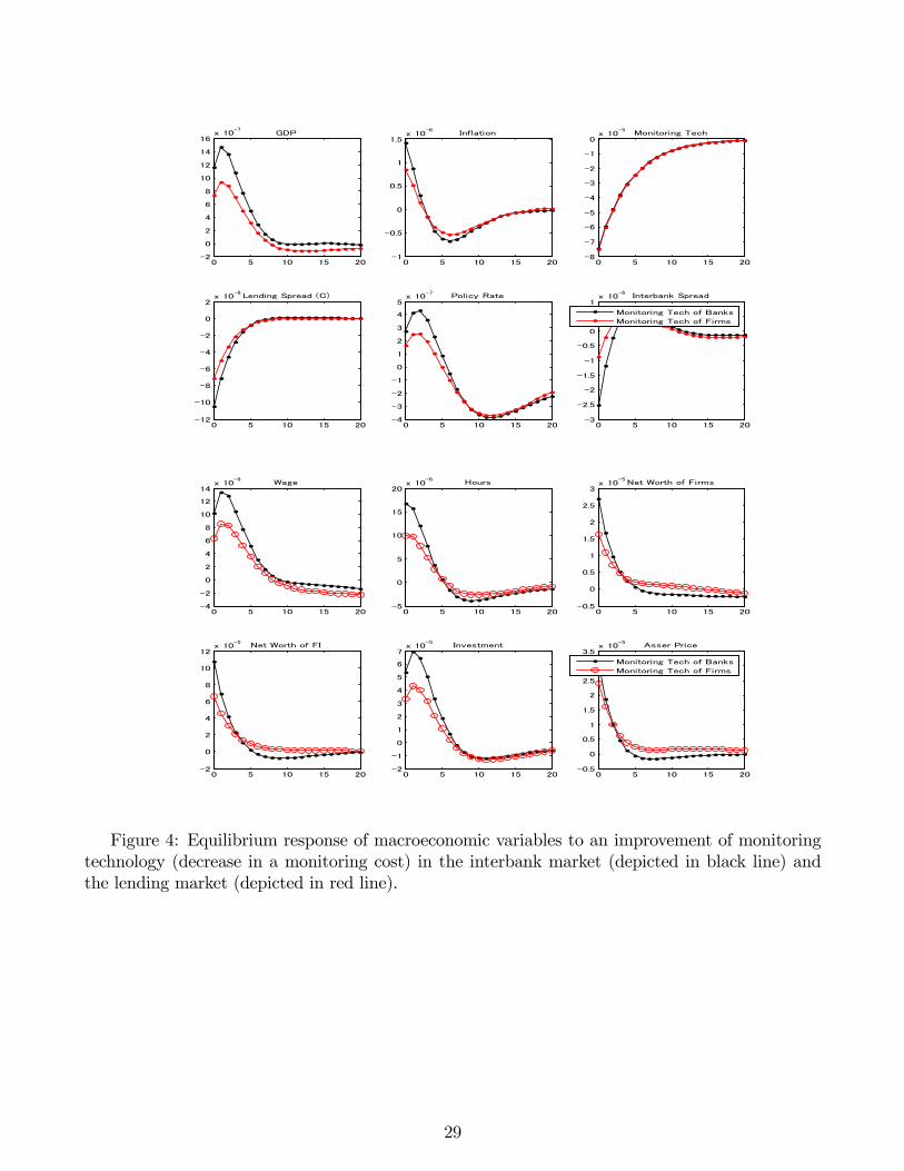
Dynamic response of an improvement in monitoring technologyWe consider a case when a reference rate is informative about a realization of !�j and provides

the range j!�j1 � !�j0 j to the lenders. As lenders spend less resources for monitoring activities, ��falls. Borrowing parameter values estimated in MSY (2012),11 we investigate both quantitativeand qualitative consequence of such changes in credit contracts. Figure 4 displays the equilibriumresponse of our model to an improvement in monitoring technology in the IF and FEC contractbrought about by a short-run decline in �F and �c: As indicated in Figure 3, defaulting probabilityof borrowers being unchanged, a smaller monitoring cost �F leads to a lower expected default costsconfronting investors. Consequently, the credit spread in interbank rF (st+1jst) � R (st) shrinks.

10Following Christiano, Motto, and Rostagno (2009), we call this standard deviation of idiosyncratic productivity� in the borrowing sectors �riskiness.� See also Kobayashi (2012) where the reference rate is decomposed intorisk-free rate, risk premium, liquidity premium, and �uncertainty�premium.11MSY (2012) estimates the model used in this paper using the Japanese data from the 1980s to 2000s. The

parameter values are reported in Table 1.

14

Because cost of external �nancing for capital goods purchase becomes cheaper to entrepreneurs,investment grows, leading to higher GDP and in�ation.There is the second-round e¤ect stemming from endogenous developments of borrowers�net

worths. As the demand for capital goods tightens in response to the shock to the monitoringcost, asset price Q� (s

t) for � = c; x goes up. Higher asset prices together with expanding outputproduction facilitate accumulation of net worth in the FIs and goods-producing sectors, N�, for� = F; c; and x; through equations (7) and (8). The endogenous improvement of borrowers�cred-itworthiness reduces credit spreads in lending markets as well as in interbank market, facilitatinginvestment further.For the same size of decline in monitoring cost, a macroeconomic consequence of the cost decline

in the IF contract is larger than that in the FEC contracts, although the decline in the two costsyield qualitatively similar macroeconomic impacts. One reason behind this outcome is that whilea narrowing credit spread in the interbank market is easily transmitted to two credit spreads inthe lending markets through the �nancial linkage, a narrowing credit spread in the lending marketa¤ects the credit spread in the interbank only indirectly through the endogenous movements ofnet worths:12

3.2 Reference rates and borrowers�perceived idiosyncratic productiv-ity

Set upWe next discuss the channel through which reference rate a¤ects perceived uncertainty regard-

ing idiosyncratic productivity of borrowers, called riskiness, in the credit markets. Our analysis isclosely related to studies including Lucas (1972), Morris and Shin (2003), and Ui (2003). Theireconomy consists of multiple agents where each of the agents receives two separate signals, privatesignal and public signal, about the state of nature. The two signals are contaminated with noiseand agents form their expectations by solving signal extraction problem. Because all agents re-ceive the same public signal, an improvement of the public signal precision causes a cross-sectionalconvergence of agents�expectation and their actions.We introduce agents called operator into MSY (2012). There are three classes of operators

and each class of operator is attached to each of the three sectors, providing a sector speci�coperational service. There is an in�nite number of operators in each sector and an individualoperator � provides a service �ow hF;� (s

t) to a randomly chosen FI, say type i FI:We assume thatan idiosyncratic productivity of a type i FI !F;i (st) is a¤ected by the operator�s endogenous choiceof operational service amount as well as an exogenous component:

!F;i�st��

exogenous componentz }| {!Fexo;i

�st�

+

endogenous componentz }| {hF;�

�st�� hF

�st�:

Here, the exogenous component is normally distributed with zero mean and variances �2Fexo andhF (s

t) in the endogenous component is an average of operational service provided by operatorsattached to the FI sector. We assume the similar setting holds for operators attached to goods-producing sectors.Individual operator � determines its operational service hF;� (st) so as to meet the aggregate

demand �F (st) : The aggregate demand is not known to the operator and it infers the aggregate

12See Christiano, Motto, and Rostagno (2003, 2008, and 2010) for quantitative importance of shocks to riskinessin goods-producing sectors in the U.S. and euro area.

15

demand, using of two sources of information, a private signal �F;� (st) whose realization is speci�cto � and public signal F (st) that is commonly delivered to all operators. While both the signalsinclude the sum of the true value of aggregate demand �F (st) and noises vF;� (st) and $F (s

t) ; thetwo components are not observable to the operators.

�F;��st�= �F

�st�+ vF;�

�st�;

F�st�= �F

�st�+$F

�st�:

Noises vF;� (st) and $F (st) are normally distributed with zero mean and variance of �2VF and �

2$F:

Based on the statistical inference, operation service provided by the operator � conditional on therealizations of the two signals, �F;� (st) and F (st) ; is then given by

hF;��st�= E

��F�st�j�F;�

�st�;F

�st��=�F;� (s

t)�2$F+ F (s

t)�2VF�2VF + �2$F

:

While each operator is ex-ante identical, it provides a di¤erent amount of operational service fromeach other since it receives a di¤erent realization of private signals. Consequently, the signalsgenerate a divergence of operational service hF;� (st) across agencies. Because vF;� (st) is normallydistributed with variance of �2VF , cross-sectional variance of operators�operation service is givenby Z 1

0

�hF;�

�st�� hF

�st��2

d� =�2VF�

�2VF =�2$F+ 1�2 :

Clearly, the FIs�riskiness, the cross-sectional standard deviation of operational service, is increas-ing function of variance of the noise contained in public signal. The riskiness of the FI is thereforegiven by

�2F�st�= �2Fexo

�st�+

�2VF (st)�

�2VF =�2$F+ 1�2 : (22)

When public signal increases its accuracy about aggregate demand for operational service, there-fore, a cross-sectional variance of operational services becomes smaller, reducing the riskiness ofthe FI sector. The similar mechanism holds in the goods-producing sectors.

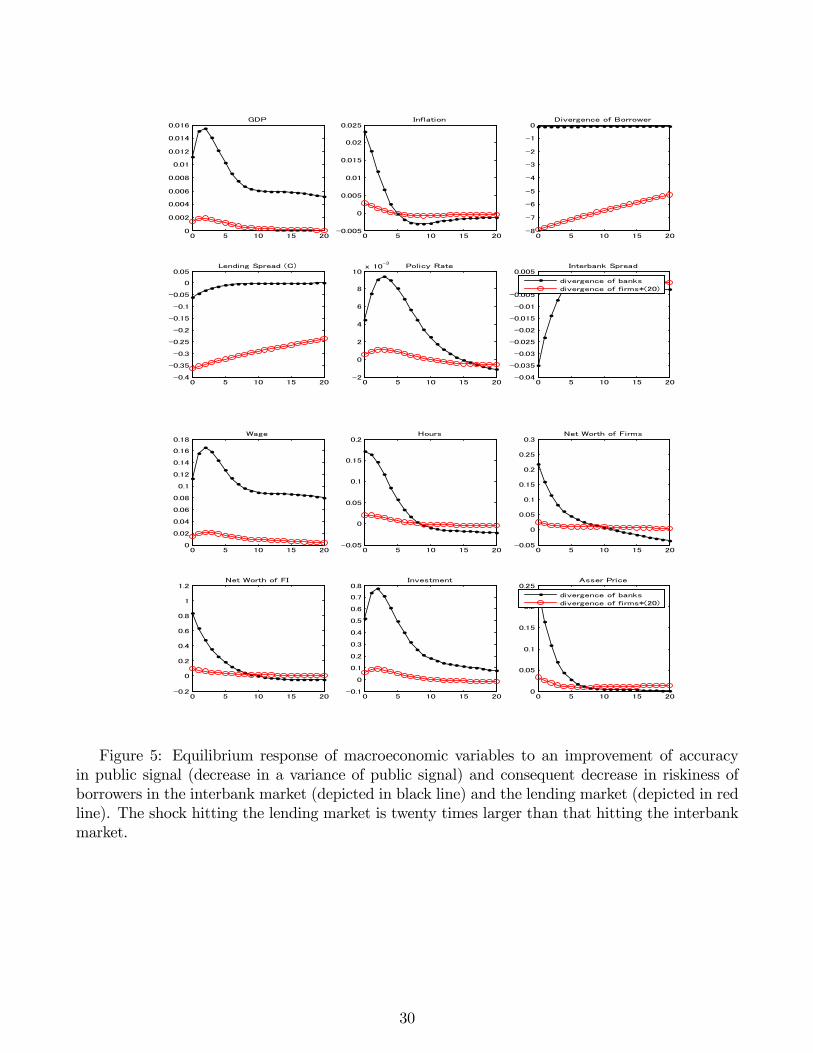
Economic response to an improvement in public signalFigure 5 displays the equilibrium response of macroeconomic variables to a temporary decline of

riskiness in the interbank market �2F driven by an improvement of reference rate �2$F. As it lowers

an expected portion of defaulting borrowers in interbank market, the interbank spread rf (st+1jst)� R (st) narrows, making a external �nance for capital goods purchase cheaper. Consequently,investment and output grow and in�ation increases. The second round e¤ect is also present. Theendogenous developments of the net worths in the borrowers of the credit markets help furtherreduce credit spreads, boosting the economy. The �gure also displays the equilibrium response ofour model to a temporary decline of riskiness in the lending market �2c . Similarly to the consequenceof reduced monitoring costs �F and �c; changes in the two riskiness bring about qualitatively thesame impacts on the economy, though macroeconomic impacts caused by the decline in �2F issubstantially larger compared to the one caused by the decline in �2c :

13

13In this paper, we investigate the economic response to a unexpected decline in monitoring cost and riskinessand display that such shocks boost the economy. Clearly, if the degree of informational friction increases becauseof the changes in these parameters in the opposite direction, then output is instead dampened. See Heider et al.(2009) for the discussion that relate informational friction and surge in the credit spread during the �nancial crisis.

16

4 Reference rates as a tool of expectation management

In this section, we discuss the role of reference rates in expectation formation and business cy-cle �uctuations. To do this, we extend the literature of �Pigou cycle,� including Pigou (1926),Beaudry and Portier (2006), and Jaimovich and Rebelo (2009). These studies shed the light on theanticipated shock as a distinct source of business cycle �uctuations from unanticipated shocks thathave been considered as the key determinants of the business cycle �uctuations. Agent in theirmodels receives news regarding future events such as an exogenous rise in the goods productiontechnology that will occur several quarters ahead. Since the agent�s economic decision today isa¤ected by his/her expectation, current economic variables are dependent upon the way that agentresponds to the news. In particular, recent studies along this line estimate a DSGE model thatincorporates anticipated shocks and document that such news shocks are quantitatively importantdrivers of the business cycle �uctuation in the U.S. and in Japan (Fujiwara, Hirose, and Shintani2009; and Schimitt-Grohé and Uribe; 2012).Similarly to the discussions in Section 3, we discuss the role of reference rate in expectation

formation by introducing an additional setting to MSY (2012). We speci�cally consider news thatinforms agents that there will be an exogenous change in the FIs�net worth in the future. Incontrast to standard treatment of news in the literature where quantity of the economic event,such as the size of productivity increase, is perfectly foreseen, news in our economy is contaminatedwith noises. As agents are only certain about the timing of the event but uncertain about the sizeof the event, they predict the size using a statistical inference. Consequently, agents�expectationregarding the net worth shock does not necessarily match with what materializes in the future.The discrepancy between the predicted size of net worth change and the materialized size acts asan additional source of business cycle �uctuations in the economy.

Set upWe assume that agents in the economy receive news in period t that informs them that there

will be an exogenous change in FIs�net worth by �nF in the two years horizon, in period t + 8:When the news arrives in period t; therefore, agents expect that a net worth in t + 8 evolvesaccording to

NF

�st+8

�= FVF

�st+7

�+ "NF

�st+7

�+

WFc (st+7)

PCPI (st+7)+WFx (s

t+7)

PCPI (st+7)+ Et

��nF

�st+8

��:

Agents know that there is a change in the net worth, but they do not know its size with certainty.In addition to the news, agents receive two signals in period t, private signal and public signal,denoted by �F (st) and F (st) ; respectively. Both two signals are the sum of the true value offuture net worth change �nF (st+8) and disturbances vF (st) and $F (s

t) :

�F�st�= �nF

�st+8

�+ vF

�st�;

F�st�= �nF

�st+8

�+$F

�st�:

Similarly to the setting in Section 3, these disturbances vF;� (st) and $F;� (st) are normally distrib-

uted with zero mean and variance �2VF and �2$F; respectively, and these statistical properties of

the disturbances are known to agents.Agents only observe realization of the signals and do not observe each of the two components.

Making use of the statistical properties of disturbances, they forecast the size of future exogenousnet worth change �nF (st+8) based on the statistical inference:

17

E��nF

�st+8

�j�F

�st�;F

�st��=�F (s

t)�2$F+ F (s

t)�2VF�2VF + �2$F

:

The above equation indicates that an expected value of exogenous net worth change conditionalon information available today is a¤ected by the variance of public and private signals �2VF ; �

2$F.

It further indicates that, other things being equal, as variance of public signal �2$Fis reduced,

the discrepancy between expectation and realization regarding the net worth change diminishes.While such a discrepancy itself works as an innovation to the economy, the accuracy of expectationbrought about by the reliable public signal help mitigate economic �uctuations stemming from theinnovation.

Quantitative role played by a reliable public signal in stabilization economic �uc-tuationsWe then quantitatively investigate the role of public signal in stabilizing macroeconomic �uc-

tuation through its guidance of agents�expectation formation. We start from a simple example,comparing two cases; a case when an exogenous net worth change materializes exactly in the waythat it was expected (case i) and a case when the net worth change does not materialize eventhough it was expected to occur (case ii). Mathematical formulations of those two cases are givenby the following two equations:

case i : �nF�st+8

�= E

��nF

�st+8

�j�F

�st�;F

�st��= �1;

case ii : �nF�st+8

�= 0 6= E

��nF

�st+8

�j�F

�st�;F

�st��= �1:

Note that the two scenarios are identical in terms of agents�expectation formation about the sizeof exogenous net worth change and di¤er in the materialization of the net worth changes.Figure 6 displays the equilibrium response of the economy to the news under the two scenarios.

In both cases, at the arrival of the news, entrepreneurs expect that they are going to face ahigher borrowing rate in the two years horizon as credit spread widens re�ecting an exogenousdisruption of FIs�net worth by�nF (st+8). Because the expected borrowing rate rises, the expectedinvestment demand falls, leading to a fall in current asset price Qc (s

t). The fall in current assetprice reduces current net worth in both FI and goods-producing sectors through equations (7) and(8), widening current credit spreads and dampening current investment, output, and in�ation.The equilibrium time paths under the two scenarios, the case i and the case ii, are identical upuntil period t+8 in the period when the news materializes. Under the case i, since the exogenousdeterioration of net worth occurs in the way that it was expected, agents have already take thedeterioration into consideration. Consequently, no surprise takes place in the economy. Althoughthe net worth of FI displays a sharp decline in the period, macroeconomic variables evolve smoothlyover the period of materialization and beyond. Under the case ii, exogenous deterioration of networth does not materialize in period t + 8; even though agents expect that such deteriorationoccurs. This is conceived as a positive surprise to the agents in the economy. Consequently,asset price Qc (s

t+8) upsurges, driving output and in�ation upward, yielding a volatile economic�uctuations compared to the case ii. Clearly, what plays the part is the accuracy of expectationformation in stabilization of the economy.Next, we discuss two other scenarios where materialized size of the net worth change is the

same across scenarios while the expectations regarding the size of the changes are di¤erent. Inthe case iii, agents expect a unit decline in FIs�net worth and the materialized exogenous changein the FIs�net worth is half of its prediction. In case iv, agents accurately predict that size of

18

exogenous net worth change in two years ahead. Again, formulations of the two cases are shownas below:

case iii : �nF�st+8

�= �0:5 6= E

��nF

�st+8

�j�F

�st�;F

�st��= �1;

case iv : �nF�st+8

�= �0:5 = E

��nF

�st+8

�j�F

�st�;F

�st��:

Figure 7 displays the equilibrium response of the economy to the news under the two scenarios.In contrast to the two scenarios displayed in Figure 6 where agents form the same expectation,the equilibrium time paths under case iii and iv are di¤erent throughout the simulation period.Since agents under case iv expect a smaller decline in the net worth than agents under case iii,adverse impacts of the news on the macroeconomic activity are moderate up to period t + 8 inthe former scenario. In period t + 8; a net worth declines with the same size materializes in thetwo scenarios. In case iii, since the exogenous net worth decline turns out to be smaller thanexpected, the discrepancy between the expected change and materialized change is conceived asan expansionary shock to the agents in the materialized period. Consequently, output, in�ation,and other macroeconomic variables suddenly jump up at the period.The analysis above indicate that accuracy in agents�expectation regarding future shocks con-

tributes to a stabilization of the macroeconomy. To see this in details, we gauge the variationsof macroeconomic variable x conditional on the news arrival �2x; by taking average of squareddeviation from its steady state value �xt over �ve years horizon after the news arrival;

�2x =20Xt=0

(�xt)2 :

Table below documents a size of the variations �2x under four scenarios where agents�expectationconditional on the news is -2, -1, 0, and 1, respectively, and the net worth change that materi-alizes 8th quarter after the news is all -0.5. For illustrative purpose, all variations are dividedby the variations �2y;iv that is measured under the scenario iv where realization of the net worthchange exactly matches with the agents�expectation. As the absolute value of discrepancy betweenthe expected size and materialized size of the net worth change widens, the measured volatilitymonotonically increases for all four macroeconomic variables, output, in�ation, labor input, andvalue-added produced from the durables sector (sum of consumer durable expenditure and invest-ment), indicating that the improvement in economic outlook thanks to a reliable reference ratebrings about the macroeconomic stabilization.

�2y=�2y;iv �2�=�

2�;iv �2l =�

2l;iv �2I=�

2I;iv

E [�nF (st+8) j�F (st) ;F (st)] = �2 10.41 27.48 17.97 13.38E [�nF (st+8) j�F (st) ;F (st)] = �1 2.46 5.06 2.90 2.95E [�nF (st+8) j�F (st) ;F (st)] = 0 1.24 1.72 2.86 1.22E [�nF (st+8) j�F (st) ;F (st)] = 1 6.77 17.50 17.84 8.20

5 Reference rates as a disturbance to monetary policy im-plementation

Set up

19

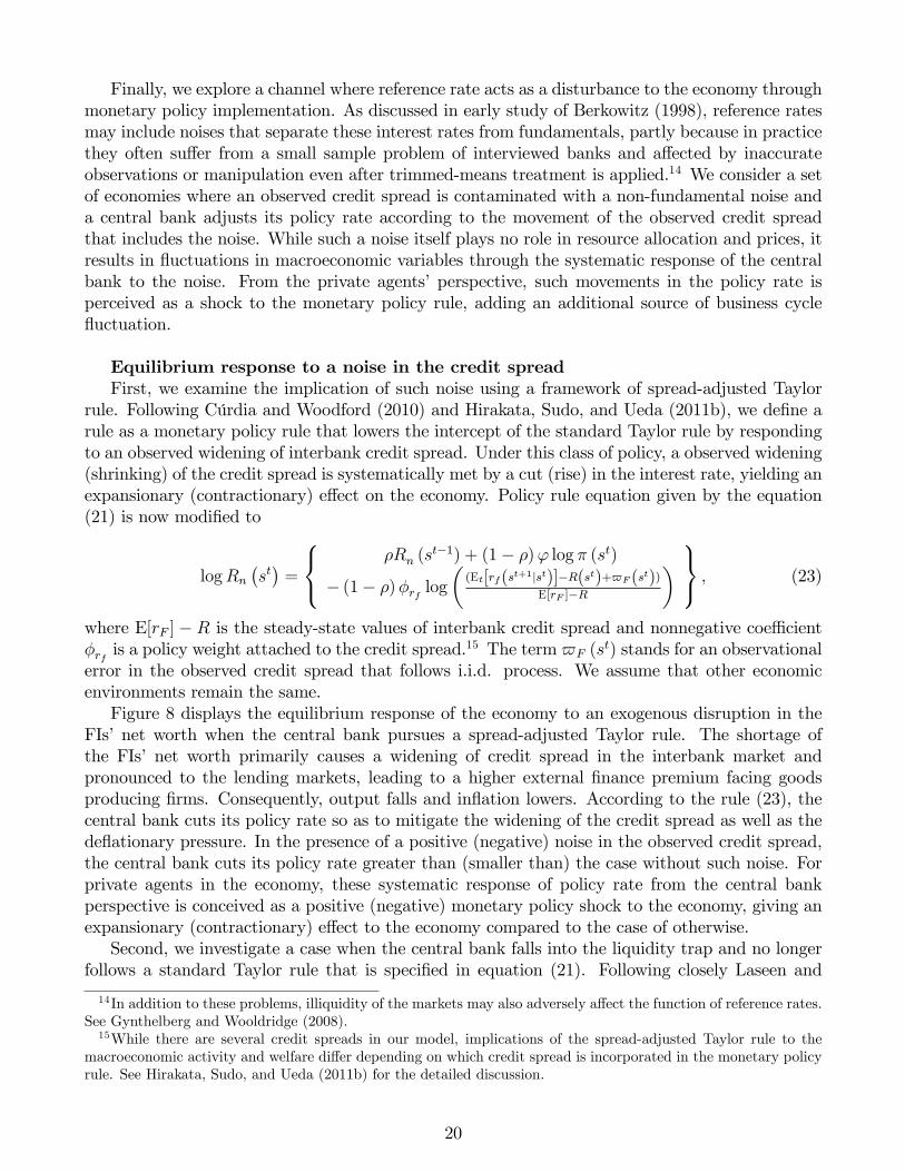
Finally, we explore a channel where reference rate acts as a disturbance to the economy throughmonetary policy implementation. As discussed in early study of Berkowitz (1998), reference ratesmay include noises that separate these interest rates from fundamentals, partly because in practicethey often su¤er from a small sample problem of interviewed banks and a¤ected by inaccurateobservations or manipulation even after trimmed-means treatment is applied.14 We consider a setof economies where an observed credit spread is contaminated with a non-fundamental noise anda central bank adjusts its policy rate according to the movement of the observed credit spreadthat includes the noise. While such a noise itself plays no role in resource allocation and prices, itresults in �uctuations in macroeconomic variables through the systematic response of the centralbank to the noise. From the private agents�perspective, such movements in the policy rate isperceived as a shock to the monetary policy rule, adding an additional source of business cycle�uctuation.

Equilibrium response to a noise in the credit spreadFirst, we examine the implication of such noise using a framework of spread-adjusted Taylor

rule. Following Cúrdia and Woodford (2010) and Hirakata, Sudo, and Ueda (2011b), we de�ne arule as a monetary policy rule that lowers the intercept of the standard Taylor rule by respondingto an observed widening of interbank credit spread. Under this class of policy, a observed widening(shrinking) of the credit spread is systematically met by a cut (rise) in the interest rate, yielding anexpansionary (contractionary) e¤ect on the economy. Policy rule equation given by the equation(21) is now modi�ed to

logRn

�st�=

8<: �Rn (st�1) + (1� �)' log � (st)

� (1� �)�rf log

�(Et[rf(st+1jst)]�R(st)+$F (st))

E[rF ]�R

� 9=; ; (23)

where E[rF ] � R is the steady-state values of interbank credit spread and nonnegative coe¢ cient�rf is a policy weight attached to the credit spread.

15 The term $F (st) stands for an observational

error in the observed credit spread that follows i.i.d. process. We assume that other economicenvironments remain the same.Figure 8 displays the equilibrium response of the economy to an exogenous disruption in the

FIs�net worth when the central bank pursues a spread-adjusted Taylor rule. The shortage ofthe FIs� net worth primarily causes a widening of credit spread in the interbank market andpronounced to the lending markets, leading to a higher external �nance premium facing goodsproducing �rms. Consequently, output falls and in�ation lowers. According to the rule (23), thecentral bank cuts its policy rate so as to mitigate the widening of the credit spread as well as thede�ationary pressure. In the presence of a positive (negative) noise in the observed credit spread,the central bank cuts its policy rate greater than (smaller than) the case without such noise. Forprivate agents in the economy, these systematic response of policy rate from the central bankperspective is conceived as a positive (negative) monetary policy shock to the economy, giving anexpansionary (contractionary) e¤ect to the economy compared to the case of otherwise.Second, we investigate a case when the central bank falls into the liquidity trap and no longer

follows a standard Taylor rule that is speci�ed in equation (21). Following closely Laseen and

14In addition to these problems, illiquidity of the markets may also adversely a¤ect the function of reference rates.See Gynthelberg and Wooldridge (2008).15While there are several credit spreads in our model, implications of the spread-adjusted Taylor rule to the

macroeconomic activity and welfare di¤er depending on which credit spread is incorporated in the monetary policyrule. See Hirakata, Sudo, and Ueda (2011b) for the detailed discussion.

20

Svensson (2011) and Bodenstein, Guerrieri, and Gust (2010), we consider a version of Taylor ruleexpressed in the following equation.

logRn

�st�= max

0@ �Rn (st�1) + (1� �)' log � (st)

� (1� �)�rf log

�(Et[rf(st+1jst)]�R(st)+$F (st))

E[rF ]�R

�; 0

1A : (24)

Under this rule, in the wake of adverse de�ationary shock, the central bank cuts its policy rate tozero for a period that such shock persists. As the adverse impact fades away, it then graduallyraises its policy rate to a positive value. When there is a nonzero realization of the noise $F (s

t) ;then the monetary policy implementation leads to unintended outcome by forwarding or delayingthe timing of the exit policy compared to the ideal timing targeted by the central bank.Figure 9 displays the equilibrium response of the economy to a large disruption in the FIs�net

worth. Because the size of the shock is substantially large, the policy rate following equation (24)continuously hits its �oor for several quarters after the shock. When no observational error occursin the interbank market, the central bank starts to set a positive interest rate 9th quarter afterthe adverse shock. In case that a positive noise prevails in the credit market and the observedcredit spread from central bank�s perspective is higher than the actual credit spread, the centralbank delays timing of raising its policy rate according to the policy weight attached to the creditspread. In this example, the central bank raises interest rate in period t = 13 because of the noise.Macroeconomic consequence of the delaying in policy action is clear. Because an expansionarymonetary policy is maintained longer than a case otherwise, economy experiences a higher outputand in�ation.

6 Conclusive Remark

In recent years, particularly after the �nancial crisis, a growing attention has been paid to the roleplayed by reference rate in the economy. In contrast to existing studies that concentrate primarilyon its role in transactions in the �nancial market, in this paper, we explore what the referencerate does to the macroeconomic activity using a medium-scale dynamic general equilibrium modeldeveloped by Muto, Sudo, and Yoneyama (2012). We show that a reliable reference rate may giverise to a favorable economic outcome either through a moderation of the degree of informationalfriction in the credit markets or through an improvement of economic forecast. We also demon-strate, however, that reference rate may lead to an unintended consequence of monetary policy ifit contains a non-fundamental noise that a¤ects decision making of the central bank. Our resultsillustrate the importance of reliable reference rates in the economy particularly under the envi-ronment with economic uncertainty from the perspective of resource allocation in credit markets,macroeconomic stabilization, and policy implementation.In the current paper, we concentrate our analysis on issues about reference rate as information

tool and do not address other aspects of the reference rate. We believe, however, that there aretwo more issues regarding reference rate worth further investigation. The �rst issue is about itsinternational spillover e¤ect. When considered in open economy framework, reference rate emergesas transmitter of a country-speci�c shock in one country, say country A, to the rest of the globe.For instance, spreads in countries other than A may widen in response to a domestic noise incountry A, which is independent from creditworthiness and degree of informational friction inthese countries, and such widening of spreads lead to output �uctuations. When there is traderelationship between these countries, e¤ects of the original shock may even be pronounced. Thesecond issue is about its distributional e¤ect. As pointed out by Abrantes-Metz et al. (2012),

21

under- and overestimates of reference rates may generate net worth transfer between borrowersand lenders both within and across sectors. For instance, whenever an adverse e¤ect of a unitdecline in net worth in one sector is not equivalent to a favorable e¤ect of a unit increase in networth in the other sector, the transfer results in aggregate �uctuations.16 Exploring the role of thereference rates in details through those two dimensions is left for future research.

16HSU (2011a, b) demonstrates that a disruption in the banks�net worth causes a disproportionately large impacton the economy compared to the same size of disruption in the goods producing sector, indicating that the networth transfer across the two sectors is accompanied by the aggregate impact.

22

References

[1] Abrantes-Metz R., Kraten M., Metz A. D., Seow G. S. (2012) �Libor Manipulation?,�Journalof Banking and Finance, 36, 136 -150.

[2] Beaudry, P. Portier F. (2006) �Stock Prices, News, and Economic Fluctuations,�AmericanEconomic Review, 96, 1293-1307.

[3] Berkowitz J. (1998) �Dealer Polling in the Presence of Possibly Noisy Reporting,�FederalReserve Board Discussion Paper.

[4] Bernanke, B. S., Gertler M., Gilchrist S. (1999) �The Financial Accelerator in a QuantitativeBusiness Cycle Framework,�in Handbook of Macroeconomics, J. B. Taylor and M. Woodford(eds.), Vol. 1, chapter 21, 1341�1393.

[5] Bodenstein, M, Guerrieri L., Gust C. (2010) �Oil Shocks and the Zero Lower Bound on thenominal Interest Rate,�International Finance Papers 1009, Board of Governors of the FederalReserve System.

[6] Christiano, L., Motto, R., Rostagno, M. (2003) �The Great Depression and the Friedman�Schwartz Hypothesis,�Journal of Money, Credit and Banking 35, 1119�1198.

[7] Christiano, L., Motto, R., Rostagno, M. (2008) �Shocks, Structures or Monetary Policies? TheEuro Area and US after 2001,�Journal of Economic Dynamics and Control, 32, 2476-2506.

[8] Christiano, L., Motto, R., Rostagno, M. (2010) �Financial Factors in Economic Fluctuations,�European Central Bank, Working Paper Series, 1192.

[9] Cúdia V., Woodford M. (2010) �Credit Spreads and Monetary Policy,� Journal of Money,Credit and Banking, 42, 3-35.

[10] Fujiwara, I., Hirose, Y., Shintani, M. (2009) �Can News Be a Major Source of AggregateFluctuations? A Bayesian DSGE Approach,� Journal of Money, Credit, and Banking, 34,1-29.

[11] Gynthelberg, J., Wooldridge, P. (2008) �Interbank Rate Fixing during the Recent Turmoil,�BIS Quarterly Review.

[12] Heider, F., Hoerova, M., Holthausen, C. (2009) �Liquidity Hoarding and Interbank MarketSpreads. The Role of Counterparty Risk,�Working Paper Series 1126, European CentralBank.

[13] Hirakata, N., Sudo N. Ueda, K. (2009) �Chained Credit Contracts and Financial Accelera-tors,�Discussion Paper Series 2009-E-30, Bank of Japan.

[14] Hirakata, N., Sudo, N. Ueda, K. (2011a) �Capital Injection, Monetary Policy, and FinancialAccelerators,�Discussion Paper Series 2011-E-10, Bank of Japan.

[15] Hirakata, N., Sudo, N. Ueda, K. (2011b) �Do Banking Shocks Matter for the U.S. Economy?�Journal of Economic Dynamics and Control, 35, 2042-2063.

[16] Jaimovich, N., Rebelo S. (2009) �Can News About the Future Drive the Business Cycle?,�American Economic Review, 99, 1097-1118.

23

[17] Kawata, H., Kitamura, T., Nakamura, K., Tsuchiya S., Teranishi Y. (2012) �E¤ects and Lossand Correction in a Reference Rate on Japan�s Economy and Financial System,�Bank ofJapan Working Paper Series, 2012-E-11, Bank of Japan.

[18] Kobayashi, S. (2012) �Application of a search model to appropriate designing of referencerates: actual transactions and expert judgment,�Bank of Japan Working Paper Series, forth-coming, Bank of Japan.

[19] Kuo, D., Skeie, D., Vickerym J. (2012) �A Comparison of Libor to Other Measures of BankBorrowing Costs,�mimeo, Federal Reserve Bank of New York.

[20] Laseen, S, Svensson, L. E. O. (2011) �Anticipated Alternative Policy Rate Paths in PolicySimulations,�International Journal of Central Banking 7, 1-35.

[21] Lucas, R. E. (1972) �Expectations and the Neutrality of Money�Journal of Economic Theory,4, 103-124.

[22] Morris, S., Shin, H. S. (2002) �Social Value of Public Information,� American EconomicReview, 92, 1521�1534.

[23] Muto, I. (2012) �A Simple Interest Rate Model with Unobserved Components: The Role ofthe Reference Rate,�Bank of Japan Working Paper Series, No.12-E-10, Bank of Japan.

[24] Muto, I., Sudo, N., Yoneyama S. (2012) �Productivity Slowdown in Japan�s Lost Decade:How Much of it is Attributed to Financial Factor?,�mimeo.

[25] Pigou, A. C. (1926) �Industrial Fluctuations,�London: MacMillan and Co.

[26] Schmitt-Grohe, S., Uribe, M. (2008). �What�s �News�In Business Cycles.�Econometrica, 80,2733-2764.

[27] Snider, C., Youle T. (2010) �Does the LIBOR Re�ect Banks�Borrowing Costs?�, UCLAWorking Paper.

[28] Ui, T. (2003) �A Note on the Lucas Model: Iterated Expectations and the Neutrality ofMoney,�mimeo.

24

Table 1: Estimated and calibrated parameters used in the current model (values are taken fromMSY (2012). Estimated parameters are based on Japanese data from 1980s to 2000s.

25

Figure 1: Outline of MSY (2012).

26

0.2 0.4 0.640

50

60

70

80

90

100

nF

E t­1R tE  ­

 R

0.2 0.4 0.640

50

60

70

80

90

100

nE

E t­1R tE  ­

 R

benchmarkhigher µhigher σ

Figure 2: Credit spread EtRE (st+1jst) =R (st) as a function of creditworthiness of FIs and

goods-producing sectors, nF (st) and nE (st) ; as well as degree of informational friction governedby monitoring technology �� and standard deviation of idiosyncratic productivity �� (riskiness).

27

0.2 0.4 0.60

0.01

0.02

0.03

0.04

0.05

0.06

nF

Default Cost in IF contract

0.2 0.4 0.60

0.01

0.02

0.03

0.04

0.05

0.06

0.07

0.08

0.09

0.1

nF

Default Cost in FEC/FED contract

benchmarkhigher µhigher σ

0.2 0.4 0.60

0.01

0.02

0.03

0.04

0.05

0.06

nE

Default Cost in IF contract

0.2 0.4 0.60.03

0.04

0.05

0.06

0.07

0.08

0.09

0.1

0.11

0.12

nE

Default Cost in FEC/FED contract

Figure 3: Expected default cost ��R !�0 !�dF� (!�) in sector � as a function of creditworthiness

of FIs and goods-producing sectors, nF (st) and nE (st) ; as well as degree of informational frictiongoverned by monitoring technology �� and standard deviation of idiosyncratic productivity ��(riskiness).

28

0 5 10 15 20­2

0

2

4

6

8

10

12

14

16x 10

­7GDP

0 5 10 15 20­1

­0.5

0

0.5

1

1.5x 10

­6Inflation

0 5 10 15 20­8

­7

­6

­5

­4

­3

­2

­1

0x 10

­5Monitoring Tech

0 5 10 15 20­12

­10

­8

­6

­4

­2

0

2x 10

­6Lending Spread (C)

0 5 10 15 20­4

­3

­2

­1

0

1

2

3

4

5x 10

­7Policy Rate

0 5 10 15 20­3

­2.5

­2

­1.5

­1

­0.5

0

0.5

1x 10

­6Interbank Spread

Monitoring Tech of Banks

Monitoring Tech of Firms

0 5 10 15 20­5

0

5

10

15

20x 10

­6Hours

0 5 10 15 20­0.5

0

0.5

1

1.5

2

2.5

3x 10

­5Net Worth of Firms

0 5 10 15 20­2

0

2

4

6

8

10

12x 10

­5Net Worth of FI

0 5 10 15 20­2

­1

0

1

2

3

4

5

6

7x 10

­5Investment

0 5 10 15 20­0.5

0

0.5

1

1.5

2

2.5

3

3.5x 10

­5Asser Price

0 5 10 15 20­4

­2

0

2

4

6

8

10

12

14x 10

­6Wage

Monitoring Tech of Banks

Monitoring Tech of Firms

Figure 4: Equilibrium response of macroeconomic variables to an improvement of monitoringtechnology (decrease in a monitoring cost) in the interbank market (depicted in black line) andthe lending market (depicted in red line).

29

0 5 10 15 200

0.002

0.004

0.006

0.008

0.01

0.012

0.014

0.016GDP

0 5 10 15 20­0.005

0

0.005

0.01

0.015

0.02

0.025Inflation

0 5 10 15 20­8

­7

­6

­5

­4

­3

­2

­1

0Divergence of Borrower

0 5 10 15 20­0.4

­0.35

­0.3

­0.25

­0.2

­0.15

­0.1

­0.05

0

0.05Lending Spread (C)

0 5 10 15 20­2

0

2

4

6

8

10x 10

­3Policy Rate

0 5 10 15 20­0.04

­0.035

­0.03

­0.025

­0.02

­0.015

­0.01

­0.005

0

0.005Interbank Spread

divergence of banks

divergence of firms*(20)

0 5 10 15 200

0.02

0.04

0.06

0.08

0.1

0.12

0.14

0.16

0.18Wage

0 5 10 15 20­0.05

0

0.05

0.1

0.15

0.2Hours

0 5 10 15 20­0.05

0

0.05

0.1

0.15

0.2

0.25

0.3Net Worth of Firms

0 5 10 15 20­0.2

0

0.2

0.4

0.6

0.8

1

1.2Net Worth of FI

0 5 10 15 20­0.1

0

0.1

0.2

0.3

0.4

0.5

0.6

0.7

0.8Investment

0 5 10 15 200

0.05

0.1

0.15

0.2

0.25Asser Price

divergence of banks

divergence of firms*(20)

Figure 5: Equilibrium response of macroeconomic variables to an improvement of accuracyin public signal (decrease in a variance of public signal) and consequent decrease in riskiness ofborrowers in the interbank market (depicted in black line) and the lending market (depicted in redline). The shock hitting the lending market is twenty times larger than that hitting the interbankmarket.

30

0 5 10 15 20­0.06

­0.04

­0.02

0

0.02

0.04

0.06

0.08

0.1GDP

0 5 10 15 20­0.1

­0.05

0

0.05

0.1

0.15

0.2

0.25Inflation

0 5 10 15 20­1

­0.8

­0.6

­0.4

­0.2

0Change in Net Worth

0 5 10 15 20­0.6

­0.5

­0.4

­0.3

­0.2

­0.1

0

0.1

0.2Lending Spread (C)

0 5 10 15 20­0.06

­0.04

­0.02

0

0.02

0.04

0.06Policy Rate

0 5 10 15 20­0.35

­0.3

­0.25

­0.2

­0.15

­0.1

­0.05

0

0.05

0.1Interbank Spread

Case i

Case ii

0 5 10 15 20­0.8

­0.6

­0.4

­0.2

0

0.2

0.4

0.6

0.8

1Wage

0 5 10 15 20­1

­0.5

0

0.5

1

1.5Hours

0 5 10 15 20­0.5

0

0.5

1

1.5

2Net Worth of Firms

0 5 10 15 20­10

­5

0

5

10

15Net Worth of FI

0 5 10 15 20­3

­2

­1

0

1

2

3

4

5Investment

0 5 10 15 20­0.5

0

0.5

1

1.5

2

2.5Asset Price

Case i

Case ii

Figure 6: Equilibrium response of macroeconomic variables to an arrival of news regardingfuture disruption in the FIs�net worth for case i and case ii. The case i is a scenario when the badnews materializes two years after the arrival of the news and the case ii is a scenario when the badnews does not materialize.

31

0 5 10 15 20­0.06

­0.05

­0.04

­0.03

­0.02

­0.01

0

0.01GDP

0 5 10 15 20­0.08

­0.06

­0.04

­0.02

0

0.02

0.04

0.06

0.08Inflation

0 5 10 15 20­0.5

­0.4

­0.3

­0.2

­0.1

0Change in Net Worth

0 5 10 15 20­0.08

­0.06

­0.04

­0.02

0

0.02

0.04

0.06

0.08

0.1Lending Spread (C)

0 5 10 15 20­0.05

­0.04

­0.03

­0.02

­0.01

0

0.01

0.02Policy Rate

0 5 10 15 20­0.08

­0.06

­0.04

­0.02

0

0.02

0.04

0.06

0.08Interbank Spread

Case iii

Case iv

0 5 10 15 20­0.7

­0.6

­0.5

­0.4

­0.3

­0.2

­0.1

0Wage

0 5 10 15 20­0.5

­0.4

­0.3

­0.2

­0.1

0

0.1

0.2Hours

0 5 10 15 20­0.4

­0.3

­0.2

­0.1

0

0.1

0.2

0.3

0.4Net Worth of Firms

0 5 10 15 20­4.5

­4

­3.5

­3

­2.5

­2

­1.5

­1

­0.5

0Net Worth of FI

0 5 10 15 20­3

­2.5

­2

­1.5

­1

­0.5

0

0.5

1Investment

0 5 10 15 20­0.4

­0.3

­0.2

­0.1

0

0.1

0.2

0.3

0.4

0.5Asset Price

Case iii

Case iv

Figure 7: Equilibrium response of macroeconomic variables to an arrival of news regardingfuture disruption in the FIs�net worth for case iii and case iv. The case iii is a scenario whenagents incorrectly forecast the realization of the net worth change and the case iv is a scenariowhen agents correctly forecast the realization of the net worth change.

32

0 5 10 15 20­0.12

­0.1

­0.08

­0.06

­0.04

­0.02

0GDP

0 5 10 15 20­0.25

­0.2

­0.15

­0.1

­0.05

0

0.05

0.1Inflation

0 5 10 15 20­0.1

­0.05

0

0.05

0.1

0.15Real Interest Rate

0 5 10 15 20­0.1

0

0.1

0.2

0.3

0.4

0.5

0.6Lending Spread (C)

0 5 10 15 20­0.12

­0.1

­0.08

­0.06

­0.04

­0.02

0

0.02Policy Rate

0 5 10 15 20­0.05

0

0.05

0.1

0.15

0.2

0.25

0.3Interbank Spread

correctly estimatedunderestimated

overestimated

0 5 10 15 20­1.8

­1.6

­1.4

­1.2

­1

­0.8

­0.6

­0.4

­0.2

0Wage

0 5 10 15 20­2

­1.5

­1

­0.5

0

0.5Hours

0 5 10 15 20­2

­1.5

­1

­0.5

0

0.5Net Worth of Firms

0 5 10 15 20­14

­12

­10

­8

­6

­4

­2

0Net Worth of FI

0 5 10 15 20­6

­5

­4

­3

­2

­1

0

1Investment

0 5 10 15 20­2

­1.5

­1

­0.5

0

0.5Asser Price

correctly estimated

underestimated

overestimated

Figure 8: Equilibrium response of macroeconomic variables to a disruption of FIs�net worthunder di¤erent monetary policy regimes.

33

0 5 10 15 20­0.06

­0.05

­0.04

­0.03

­0.02

­0.01

0GDP

0 5 10 15 20­0.12

­0.1

­0.08

­0.06

­0.04

­0.02

0

0.02

0.04Inflation

0 5 10 15 20­0.04

­0.02

0

0.02

0.04

0.06

0.08Real Interest Rate

0 5 10 15 20­0.015

­0.01

­0.005

0

0.005

0.01Policy Rate

0 5 10 15 20­0.02

0

0.02

0.04

0.06

0.08

0.1

0.12

0.14

0.16True Interbank Spread

0 5 10 15 20­0.02

0

0.02

0.04

0.06

0.08

0.1

0.12

0.14

0.16Observed Interbank Spread

correctly estimated

overestimated

0 5 10 15 20­0.8

­0.7

­0.6

­0.5

­0.4

­0.3

­0.2

­0.1

0Wage

0 5 10 15 20­1

­0.8

­0.6

­0.4

­0.2

0

0.2

0.4Hours

0 5 10 15 20­1

­0.8

­0.6

­0.4

­0.2

0

0.2

0.4Net Worth of Firms

0 5 10 15 20­8

­7

­6

­5

­4

­3

­2

­1

0Net Worth of FI

0 5 10 15 20­3

­2.5

­2

­1.5

­1

­0.5

0

0.5Investment

0 5 10 15 20­1.2

­1

­0.8

­0.6

­0.4

­0.2

0

0.2Asser Price

correctly estimated

overestimated

Figure 9: Equilibrium response of macroeconomic variables to a large disruption of FIs�networth under di¤erent monetary policy regimes.

34