financial markets' appetite for risk - and the challenge ... · financial markets’ appetite...
TRANSCRIPT
IFC Bulletin No 31 221
Financial markets’ appetite for risk – and the challenge of assessing
its evolution by risk appetite indicators
Birgit Uhlenbrock1
1. Introduction
When reading a market report on how stocks fared relative to government bonds over the short run, one will often find that changes in investors’ general demand for risky assets relative to assets considered rather safe are attributed not only to changes in assets’ perceived riskiness,2 but also to investors’ average or aggregate attitude towards risk.3 Such changes in investors’ narrowly defined appetite for/aversion to risk over time might not only affect the size of the compensation market participants require per unit of risk, but could also influence how markets react to shocks. Bad news in a market situation where investor risk appetite is already low is likely to result in a much greater repricing of risky assets than in periods where it is high. The dynamic stance of the risk appetite of market participants as a sentiment could thus serve as an important contributing factor in the transmission of shocks through the financial system. Furthermore, as it might itself be influenced by the situation in financial markets, it could work as a multiplier. Accordingly, taking into account the risk appetite/risk aversion of investors and its evolution has become an important element of assessing the condition and stability of financial markets.
A number of indicators have therefore been proposed in the literature for quantifying the evolution of investors’ general risk appetite (for an overview see eg Illing and Aaron (2005)). Some of them are based on theoretical models, while others are more atheoretic or ad hoc in the sense that they only aggregate the information contained in market data without relying on a theoretical framework. But the notion of risk appetite underlying these indicators is not necessarily identical. Under a narrow interpretation of risk appetite, one faces the difficulty of having to disentangle the effects of changes in investors’ risk appetite on investors’ relative demand for risky assets from those of changes in risk assessments. For this, one can try to
1 Address: Deutsche Bundesbank, Central Office, Markets Department, Wilhelm-Epstein-Strasse 14,
60431 Frankfurt am Main, Germany; e-mail: [email protected].
I would like to thank Thilo Liebig, Klaus Düllmann, Heinz Herrmann, and in particular Joachim Grammig for their helpful comments. Nevertheless, the views expressed in this paper represent my personal opinions and do not necessarily reflect the views of the Deutsche Bundesbank or its staff.
2 In a stochastic environment, a priori the total return on an initial investment will generally be uncertain and subject to various kinds of risk, such as market risk, liquidity risk, and default risk. Assuming that changes along such risk dimensions lead to an immediate repricing of assets in financial markets, in the sections below, the asset (return) riskiness measure of interest will be based on variances or covariances of (relatively short-term) realised asset returns.
3 Traditionally, models often assume that an individual investor’s fundamental degree of risk aversion is a characteristic parameter that remains constant. But this does not preclude a change at the aggregate (cross section) level if eg investors are not all identical, but are characterised by different individual degrees of aversion to risk, and if the composition of investors actively participating in the markets changes over time, see Kumar and Persaud (2002). Furthermore, the behavioural finance theory argues that the degree of risk aversion of an individual investor may also change over time depending on previous investment decisions’ outcomes. Thus, a row of positive results might cause an investor to become overconfident and less averse to taking on risk, while the opposite may happen after significant losses.
222 IFC Bulletin No 31
rely on particular modelling assumptions when developing indicators. Alternatively, one may choose to circumvent the problem by simply focusing on the combined effects reflected in changes of the relative demand for risky assets. This leads to indicators for a more broadly defined concept of risk appetite. Finally, in theory the stance of investors’ general risk appetite is likely to affect all risky financial market segments. In terms of actual results, however, the various risk appetite indicators often vary in their coverage of financial market segments, which is another potential source of heterogeneity.
It is therefore maybe not altogether surprising that the different indicators do not always suggest a similar stance of investors’ risk appetite. What is even more problematic, it might not always be one that coincides well with given priors around critical periods in financial markets (see eg Illing and Aaron (2005)). Such findings raise concern about the usefulness of applying risk appetite indicators in the first place. A better understanding of how individual indicators work thus seems clearly warranted and might offer ways of potential improvement down the road. The paper contributes to this evolution, concentrating on the so-called Global Risk Appetite Index (GRAI) class of indicators.
This indicator concept, originally developed by Kumar and Persaud (2002), rests on the assumption that at a given point in time the price of a risky asset will already reflect an assessment of its risk. The authors assume that a significant monotonic relationship between excess returns and past measures of perceived riskiness for a cross section of risky assets should then be observed only if markets participants’ aggregate risk appetite has changed. Focusing on the foreign exchange market segment, Kumar and Persaud (2002) assess the significance of risk appetite changes using cross-sectional Spearman rank correlation coefficients between monthly or quarterly excess returns of assets and assets’ past volatilities.4 Conversely, Wilmot, Mielczarski et al (2004) and the Deutsche Bundesbank (2005) assume linear relationships between excess returns and past riskiness. Furthermore, they apply a linear-regression indicator approach to data from not only one financial market segment at a time, but considering stock and bond markets together. Finally, to emphasise investors’ aggregate risk aversion as the dual concept to risk appetite, Coudert and Gex (2006) choose to define their linear Global Risk Aversion Index as the negative of the cross-sectional linear correlation between excess returns of assets and past volatilities.5
Its intuitiveness and simplicity makes the GRAI class a popular choice among the theory-based risk appetite indicators. The ability to cover a larger cross section of indices from several financial market segments in an integrated way is another attractive feature. However, one also has to keep in mind some caveats. Despite having a similar model in mind, (G)RAI indicator results will also finally depend on particular specification and input choices, such as the choice between a merely monotonic or a more restrictive linear relation between assets’ excess returns and measures of riskiness, the selection of assets/financial market segments, the length of the period over which to calculate the respective (excess) returns, and how to proxy for riskiness as perceived by investors. For the latter, a common practice in the literature is to rely on volatilities or variances of individual asset returns. However, in a portfolio context, this effectively amounts to assuming that covariances
4 They applied their indicator to specific segments of financial markets, primarily the FX market, but also to the
US stock market, where they examined a cross section of US sector equity indices. For details, see Kumar and Persaud (2002), p 414. To avoid any overlap of the period over which volatilities and returns were calculated, the volatilities were derived for a period of 250 business days prior to the excess return period.
5 For their linear correlation-based index they used the abbreviation GRAI, while the negative corresponding cross-sectional regression coefficient was dubbed Risk Aversion Index (RAI). They applied the indicators to two sets of cross-sectional data (one of foreign exchange rates, and another of international stock indices) separately like Kumar and Persaud (2002); however, they used a lower frequency of monthly rather than daily data.
IFC Bulletin No 31 223
between asset returns do not significantly contribute to the riskiness of assets.6 Misina (2006) therefore suggests taking the full variance-covariance (VCV) matrix of asset returns into account in his extended factor-based rank-correlation risk appetite indicator, called RAI-MI. Since he wanted to compare results of his RAI-MI with the preferred indicator of Kumar and Persaud (2002), however, his paper focused on international FX markets.
The present paper broadens the investigation into the relative pros and cons of the Misina factor extension, as well as the other necessary choices to be made when deriving a GRAI-type risk aversion indicator. However, we introduce an important additional restriction to the Misina (2006) factor extension, which leads to our modified version of the factor-extended rank-correlation Global Risk Aversion Index (F-GRAI).
The remainder of the paper is organised as follows: the next section contains a short presentation of the theoretical background to the GRAI class of risk appetite indicators. Section 3 then moves on to an empirical analysis of the GRAIs as global risk aversion indicators, where in terms of financial market coverage we focus first on international stock markets and later on stock and bond markets combined. The recent stressful phase of financial market turmoil from mid-2007 onwards serves as an important yardstick for evaluating the plausibility of results and how that is affected by the factor extension as well as the other implementation decisions.7 Finally, Section 4 summarises the main results.
2. Methodology: the GRAI indicator – theoretical motivation and the Misina critique
Apart from adding the assumption that “investors have the same, but changing risk appetite”, Kumar and Persaud (2002) in principle rely on a simplified capital asset pricing model (CAPM)8 for theoretically motivating their indicator’s key hypotheses. These are that a rank correlation between a cross section of asset price movements at time t and the assets’ riskiness at t – m should be weak for a contemporary change in general risk, but strong for a change in the general appetite for risk. With some measure of volatility as a proxy of asset riskiness, they then used the rank correlation between asset excess returns and past volatilities from the beginning of the return period as their risk appetite indicator.
Under the usual assumptions of the CAPM, the expected return of a risky asset i in period t + 1, +1( )i
tE R , in equilibrium should exceed the risk-free rate +1ftR by a risk premium (excess
return) equal to the representative investor’s degree of risk aversion ρ times the asset’s systematic risk. Since the latter is determined by how the asset return covaries with the return +1
MtR of the market portfolio, this gives the familiar equation:
ρ ρ σ+ + + +− = = ⋅1 1 1 1 ,( ) cov( , )i f i Mt t t t i ME R R R R . (1)
6 In the portfolio context that might be used to motivate the GRAI class of indicators theoretically, asset returns’
covariances will be zero in the case of independence, see also Coudert and Gex (2006). 7 Of course, another interesting empirical question in terms of the usefulness of a risk appetite indicator might
be to explore whether factors that are considered influential for the evolution of investors’ risk appetite, eg the degree of liquidity in financial markets, can be related to the dynamic evolution of investors’ aggregate risk appetite over time. See eg ECB (2007a).
8 For details on their simplified version of a CAPM, see Kumar and Persaud (2002), p 409 ff. However, the CAPM model used below is closer to eg Coudert and Gex (2006).
224 IFC Bulletin No 31
A portfolio return is the sum of the returns on the portfolio’s individual assets times their given portfolio weightsα i , ie α+ += ⋅∑1 1
M it i t
iR R , with α =∑ 1i
i. The covariance σ ,i M can thus be
rewritten as
σ α σ α σ σ σ+ + + + +≠
= = ⋅ + ⋅ = =∑2 2, 1 1 1 1 1cov( , ) , with var( ) and cov( , )i M i i j
i M t t i i j ij i t ij t tj i
R R R R R (2)
and substituted into (1) in order to obtain 2
, 1 1 1 ,( ) ( ) ( ) ( )ex ex i fi i t t t i M i i j ij
j iE R E R E R R ρ σ ρ α σ α σ+ + +
≠
= = − = ⋅ = ⋅ ⋅ + ⋅∑ . (3)
A change in expected excess returns can then arise from a change in risk aversion or a change in the riskiness of asset i stemming either from a change in its own return variance or changes in its covariances with the other asset returns in the portfolio:
ρ σρ σ
ρ σ σρ σ σ≠
∂ ∂= ⋅ + ⋅∂ ∂
∂ ∂ ∂= ⋅ + ⋅ + ⋅∂ ∂ ∂∑
,,
22
( ) ( )( )
( ) ( ) ( )
ex exex i ii i M
i M
ex ex exi i i
i ijj ii ij
E R E RdE R d d
E R E R E Rd d d (4)
According to (4), an autonomous change in the degree of risk aversion ρ should thus produce a change of asset excess returns in proportion to their riskinessσ ,i M ,
σρ
∂ = ∀∂ ,( ) ,
exi
i ME R i . (5)
In the model, a change in risk aversion should therefore be accompanied by a significant correlation between asset excess returns and their riskiness. However, for an empirically feasible GRAI indicator, observable proxies must be substituted for the quantities on both sides of (5). Changes in expected asset returns are thus replaced by short-term realised (ie ex post) returns defined in terms of observed changes in log asset prices.9 The practice of approximating asset return riskiness by their own past volatilities or variances alone, as in Kumar and Persaud (2002), may lead to a different ranking of assets in terms of riskiness than if one considered the covariances with the market portfolio, however. As shown by equation (2), only for covariances between the individual asset returns equal to zero and asset weights either equally large or increasing with the asset return variances it would be guaranteed that both approaches give the same asset return riskiness rankings. Misina (2003) argues, however, that the independence of asset returns has a further benefit when applying the GRAI. For independent returns, a common shock to the riskiness of all assets can – with given weights –occur only through a simultaneous increase or decrease of all variances. In that case, a rank correlation effect between assets’ excess returns and their past variances could not a priori be excluded, unless one assumed equally weighted portfolios (see Misina (2003), pp 15–16). However, when returns are not independent, also a change in the covariance between two asset returns could cause a rank correlation effect – again unless assets were assumed to have equal weights (see Misina (2003), p 13 ff).
9 Assuming that any repricing of assets to effect a change in risk premia takes place immediately at time t while
expectations concerning future asset values remain unchanged, one obtains = −( ( ))ex ii td E R dP . See
eg also Coudert and Gex (2006).
IFC Bulletin No 31 225
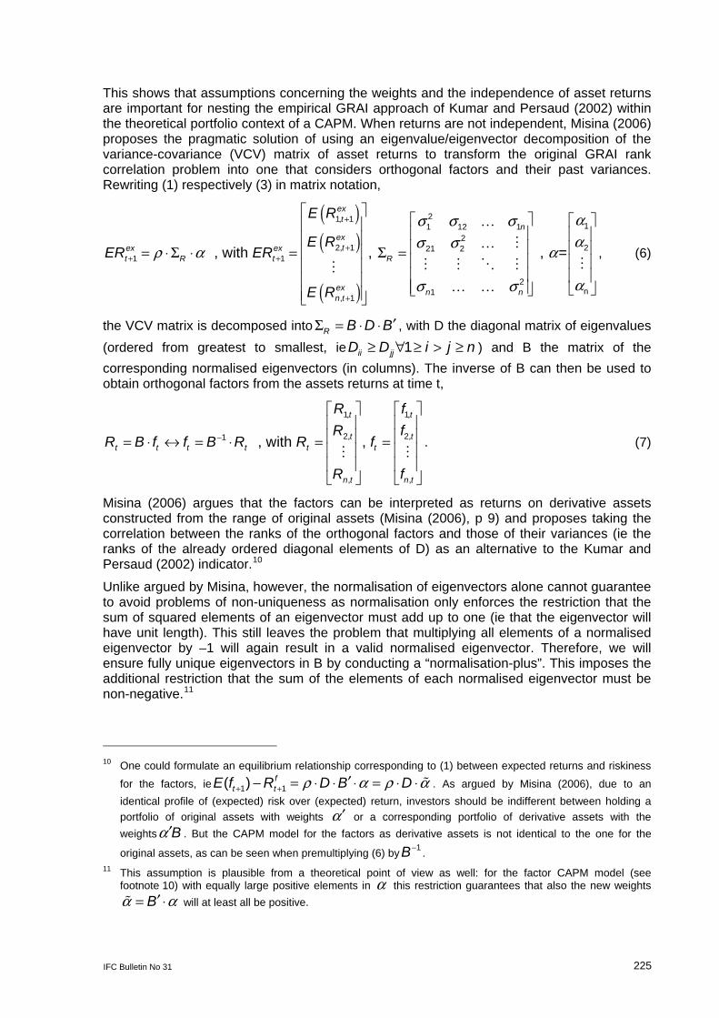
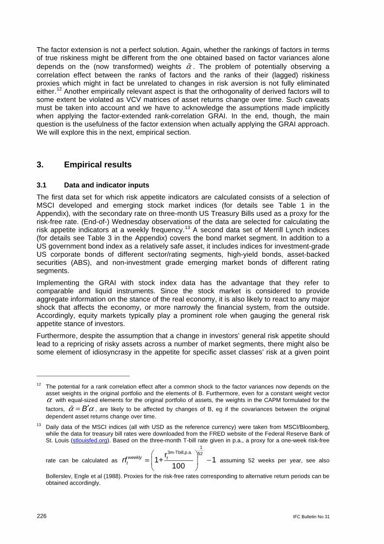
This shows that assumptions concerning the weights and the independence of asset returns are important for nesting the empirical GRAI approach of Kumar and Persaud (2002) within the theoretical portfolio context of a CAPM. When returns are not independent, Misina (2006) proposes the pragmatic solution of using an eigenvalue/eigenvector decomposition of the variance-covariance (VCV) matrix of asset returns to transform the original GRAI rank correlation problem into one that considers orthogonal factors and their past variances. Rewriting (1) respectively (3) in matrix notation,
( )( )
( )
ασ σ σασ σρ α α
ασ σ
+
++ +
+
⎡ ⎤⎡ ⎤ ⎡ ⎤⎢ ⎥⎢ ⎥ ⎢ ⎥⎢ ⎥⎢ ⎥ ⎢ ⎥= ⋅ Σ ⋅ = Σ =⎢ ⎥⎢ ⎥ ⎢ ⎥⎢ ⎥⎢ ⎥ ⎢ ⎥⎢ ⎥ ⎢ ⎥ ⎣ ⎦⎣ ⎦⎢ ⎥⎣ ⎦
K
K M
MM M O MM
K K
21, 111 12 1
22, 1 221 2
1 1
2n1
, 1
, with , , =
ext
nex
tex ext R t R
ex n nn t
E R
E RER ER
E R
, (6)
the VCV matrix is decomposed into ′Σ = ⋅ ⋅R B D B , with D the diagonal matrix of eigenvalues (ordered from greatest to smallest, ie ≥ ∀ ≥ > ≥1ii jjD D i j n ) and B the matrix of the corresponding normalised eigenvectors (in columns). The inverse of B can then be used to obtain orthogonal factors from the assets returns at time t,
−
⎡ ⎤ ⎡ ⎤⎢ ⎥ ⎢ ⎥⎢ ⎥ ⎢ ⎥= ⋅ ↔ = ⋅ = =⎢ ⎥ ⎢ ⎥⎢ ⎥ ⎢ ⎥⎣ ⎦ ⎣ ⎦
M M
1, 1,
2, 2,1
, ,
, with ,
t t
t tt t t t t t
n t n t
R fR f
R B f f B R R f
R f
. (7)
Misina (2006) argues that the factors can be interpreted as returns on derivative assets constructed from the range of original assets (Misina (2006), p 9) and proposes taking the correlation between the ranks of the orthogonal factors and those of their variances (ie the ranks of the already ordered diagonal elements of D) as an alternative to the Kumar and Persaud (2002) indicator.10
Unlike argued by Misina, however, the normalisation of eigenvectors alone cannot guarantee to avoid problems of non-uniqueness as normalisation only enforces the restriction that the sum of squared elements of an eigenvector must add up to one (ie that the eigenvector will have unit length). This still leaves the problem that multiplying all elements of a normalised eigenvector by –1 will again result in a valid normalised eigenvector. Therefore, we will ensure fully unique eigenvectors in B by conducting a “normalisation-plus”. This imposes the additional restriction that the sum of the elements of each normalised eigenvector must be non-negative.11
10 One could formulate an equilibrium relationship corresponding to (1) between expected returns and riskiness
for the factors, ie ρ α ρ α+ + ′− = ⋅ ⋅ ⋅ = ⋅ ⋅ %1 1( ) ft tE f R D B D . As argued by Misina (2006), due to an
identical profile of (expected) risk over (expected) return, investors should be indifferent between holding a portfolio of original assets with weights α′ or a corresponding portfolio of derivative assets with the weightsα′B . But the CAPM model for the factors as derivative assets is not identical to the one for the
original assets, as can be seen when premultiplying (6) by −1B . 11 This assumption is plausible from a theoretical point of view as well: for the factor CAPM model (see
footnote 10) with equally large positive elements in α this restriction guarantees that also the new weights α α′= ⋅% B will at least all be positive.
226 IFC Bulletin No 31
The factor extension is not a perfect solution. Again, whether the rankings of factors in terms of true riskiness might be different from the one obtained based on factor variances alone depends on the (now transformed) weights α% . The problem of potentially observing a correlation effect between the ranks of factors and the ranks of their (lagged) riskiness proxies which might in fact be unrelated to changes in risk aversion is not fully eliminated either.12 Another empirically relevant aspect is that the orthogonality of derived factors will to some extent be violated as VCV matrices of asset returns change over time. Such caveats must be taken into account and we have to acknowledge the assumptions made implicitly when applying the factor-extended rank-correlation GRAI. In the end, though, the main question is the usefulness of the factor extension when actually applying the GRAI approach. We will explore this in the next, empirical section.
3. Empirical results
3.1 Data and indicator inputs The first data set for which risk appetite indicators are calculated consists of a selection of MSCI developed and emerging stock market indices (for details see Table 1 in the Appendix), with the secondary rate on three-month US Treasury Bills used as a proxy for the risk-free rate. (End-of-) Wednesday observations of the data are selected for calculating the risk appetite indicators at a weekly frequency.13 A second data set of Merrill Lynch indices (for details see Table 3 in the Appendix) covers the bond market segment. In addition to a US government bond index as a relatively safe asset, it includes indices for investment-grade US corporate bonds of different sector/rating segments, high-yield bonds, asset-backed securities (ABS), and non-investment grade emerging market bonds of different rating segments.
Implementing the GRAI with stock index data has the advantage that they refer to comparable and liquid instruments. Since the stock market is considered to provide aggregate information on the stance of the real economy, it is also likely to react to any major shock that affects the economy, or more narrowly the financial system, from the outside. Accordingly, equity markets typically play a prominent role when gauging the general risk appetite stance of investors.
Furthermore, despite the assumption that a change in investors’ general risk appetite should lead to a repricing of risky assets across a number of market segments, there might also be some element of idiosyncrasy in the appetite for specific asset classes’ risk at a given point
12 The potential for a rank correlation effect after a common shock to the factor variances now depends on the
asset weights in the original portfolio and the elements of B. Furthermore, even for a constant weight vector α with equal-sized elements for the original portfolio of assets, the weights in the CAPM formulated for the factors, α α′=% B , are likely to be affected by changes of B, eg if the covariances between the original dependent asset returns change over time.
13 Daily data of the MSCI indices (all with USD as the reference currency) were taken from MSCI/Bloomberg, while the data for treasury bill rates were downloaded from the FRED website of the Federal Reserve Bank of St. Louis (stlouisfed.org). Based on the three-month T-bill rate given in p.a., a proxy for a one-week risk-free
rate can be calculated as ⎛ ⎞
= −⎜ ⎟⎝ ⎠
13m-Tbill,p.a. 52 r1+ 1
100weekly t
trf assuming 52 weeks per year, see also
Bollerslev, Engle et al (1988). Proxies for the risk-free rates corresponding to alternative return periods can be obtained accordingly.
IFC Bulletin No 31 227
in time. That is to say, one important empirical question is how informative the changes in risk appetite implied for one segment of financial markets are for the common or general risk appetite stance indicated when considering different financial market segments simultaneously. Given the implications of the subprime crisis in mid-2007, it therefore seems particularly interesting to compare the stock market GRAI with results for data sets covering only, or in addition, different bond indices. Combined data sets of stock and bond indices were also used in Wilmot, Mielczarski et al (2004) and Deutsche Bundesbank (2005). However, they looked at cross-sectional linear regressions between asset excess returns and past risk measures. Thus, one focus of the present paper is to compare the results obtained under a more restrictive linear (RAI) approach with those from the less restrictive rank-correlation GRAI approach.
There exist arguments both for and against considering different asset classes together when it comes to developing risk appetite indicators. On the one hand, a larger cross section of assets with different degrees of riskiness should, all other things being equal, lead to an increase in efficiency.14 On the other hand, assets from different asset classes will be subject to different kinds of risk. From an investor’s point of view, these kinds of risk might be more or less important at different times. The recent subprime crisis, for example, quickly put credit and liquidity risk aspects very high on investors’ worry lists. When applying the GRAI indicator to a broad cross-segment portfolio, a cross-sectional averaging effect might therefore lead to the loss of information on the risk stance towards more specific asset classes. Furthermore, the factorisation already adds another level of complexity. Expanding the data set thus might be a greater challenge to the robustness of results in the F-GRAI case. The F-GRAI also has by construction a broader range of riskiness degrees covered, it exploits the information concerning the original assets’ riskiness more efficiently.15 For the F-GRAI in particular, it might therefore not a priori be clear whether to prefer an integrated or disaggregated approach.
Apart from the choice of assets to be included in the data set, one has to make four additional central decisions to actually obtain a (G)RAI type risk appetite indicator empirically.
The first decision is how and over what length of period to calculate the (excess) returns of the assets. For the following empirical applications, the asset returns of interest are the log index changes. More precisely, the return on index i at time t is calculated as the difference between the log index values at time t and some previous time t – m, with the lag m corresponding to the chosen return period length. Excess returns are then derived by subtracting the risk-free rate for a corresponding period of length m at time t – m.
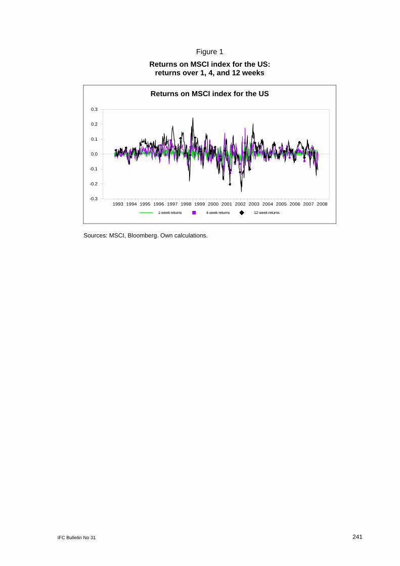
Price or valuation changes in opposite directions observed from day to day or even week to week may average out to some extent over time. On the other hand, the cumulative impact of a row of weekly changes in the same direction is more visible if returns are calculated over a longer period. The pattern of returns thus becomes smoother and more distinguishable for longer return periods (see also Figure 1 in the Appendix). Accordingly, quarterly or even six-month returns are often preferred when implementing a (G)RAI type of risk appetite indicator, since a smoother GRAI seems easier to interpret (see eg also Coudert and Gex (2006) and Deutsche Bundesbank (2005)). Unless otherwise noted, we therefore focus on the (G)RAI results obtained for a longer return period of 12 weeks.
14 Kumar and Persaud (2002), p 413, suggest using as many asset returns and as long a history as possible in
order to reduce the risk of a chance correlation between risks and returns. 15 As Wilmot, Mielczarski et al (2004) argue, their approach rests on the availability of a set of assets that differ
sufficiently in terms of their degrees of riskiness. But using the factorisation approach, derivative assets are constructed that cover a much broader range of degrees of riskiness (in terms of the difference between maximum and minimum riskiness) than the original range of assets.
228 IFC Bulletin No 31
A second decision has to be made regarding how to proxy for assets’ riskiness. This holds true even when deciding to use lagged asset return variances (ie variances calculated at time t – m) as proxies, as in the empirical GRAI literature. Intuitively, a 12-week return period might suggest considering the lagged variances of 12-week asset/index returns as well. However, to calculate the variance of 12-week returns from non-overlapping observations, one would need at least 7–9 years of data (30–39 observations). While this is the statistically correct approach, once one allows for changing variances, one may question whether such a measure, in which current developments can have only minimal impact, is a good proxy for an asset’s riskiness as perceived by real-life investors. Therefore, the GRAI literature typically considers a much shorter window of asset return observations for calculating volatilities/variances. Kumar and Persaud (2002), for example, use one year of daily data.
In the current situation, one might thus decide to use the variance of weekly returns calculated for a short window of 52 weeks, but appropriately scaled to match the return-period length, as an alternative. While a long-term risk concept seems more relevant for a long-term portfolio investor, over the shorter periods of the GRAI context the scaled proxy certainly holds a particular appeal, too.16 Because a return over 12 weeks might be approximated by the sum of the one-week returns over the respective 12 weeks, an alternative is to construct an approximate measure for the 12-week return variance via a temporal aggregation approach.17 For estimating an approximate 12-week return VCV matrix at time t, this approach takes into account the covariances between weekly returns at different lag lengths in addition to the most recent and lagged estimates of the VCV matrix of weekly returns. The simple scaling of variances, on the other hand, focuses only on the most recent information regarding short-term asset return riskiness. A priori it is not clear which approach might be preferable in the current context. Hence, we apply both the scaling and the temporal aggregation approach to the construction of asset return variances and covariances. For the construction of the GRAIs, the estimated variances and VCV matrices of asset returns are then appropriately lagged to avoid any overlap with the period over which the cross section of asset excess returns is calculated.
As argued above, however, even when assuming equal portfolio weights for the different assets, the riskiness of asset returns does not only depend on asset returns’ own variances, but also on their covariances. While Misina (2006) suggests deriving factors from dependent asset returns and an eigen decomposition of the asset return VCV matrix, the true VCV matrix is unknown and may even change over time. Accordingly, the historical VCV matrix calculated at time t – m is used as an appropriately lagged, but ex post necessarily imperfect estimate in the factorisation step. This implies, however, that the factor portfolio returns actually realised for time t are no longer guaranteed to be independent by construction. However, one can still expect that the problem of dependence between returns is smaller with than without the factorisation adjustment.
Based on the decomposition of the lagged asset return VCV matrix estimate ′Σ = ⋅ ⋅R B D B (with B as the matrix of “normalised-plus” eigenvectors in columns), the factors corresponding to the observed original asset returns at time t are thus calculated as
16 Furthermore, if changes in the implied or revealed risk appetite behaviour of investors at least partly reflect the
changes in riskiness seen over a shorter period, longer-term measures of variances – while being less variable proxies – might not resolve the real identification issue of capturing the evolution of riskiness as perceived by the average investor either.
17 See in this context eg also Brandt (2008), p 16.
IFC Bulletin No 31 229
−
⎡ ⎤ ⎡ ⎤⎢ ⎥ ⎢ ⎥⎢ ⎥ ⎢ ⎥= ⋅ = =⎢ ⎥ ⎢ ⎥⎢ ⎥ ⎢ ⎥⎣ ⎦ ⎣ ⎦
M M
1, 1,
2, 2,1
, ,
, with ,
t t
t tt t t t
n t n t
R fR f
f B R R f
R f
.
As in Misina (2006), the correlation between the ranks of the factors and the ranks of their lagged variances (ie the respective diagonal elements of the matrix D) is then used for the factor-based GRAI indicator.
However, this step actually involves another decision, namely whether to calculate the risk appetite or aversion indicator assuming a linear or a monotonic relationship between the cross section of asset excess returns at some time t and appropriately lagged past measures of their riskiness. The former corresponds to a linear cross-sectional correlation or regression approach, the latter to the Spearman rank correlation approach of Kumar and Persaud (2002) (see also Misina (2006), p 5). In the following presentation of empirical results, GRAI stands for a rank correlation indicator and RAI for the linear RAI indicator, either as a linear correlation (RAI-C) or linear regression version (RAI-R). The usage of asset excess returns or factor returns, if not otherwise noted, is indicated by adding the prefix R- or F- to the indicator abbreviation. To emphasise the dual concept of changes in risk aversion rather than risk appetite, the respective cross-sectional regression or correlation coefficient estimates are multiplied by –1 so that positive values correspond to increases in risk aversion (see Coudert and Gex (2006)). Our (G)RAIs therefore represent global risk aversion indicators.
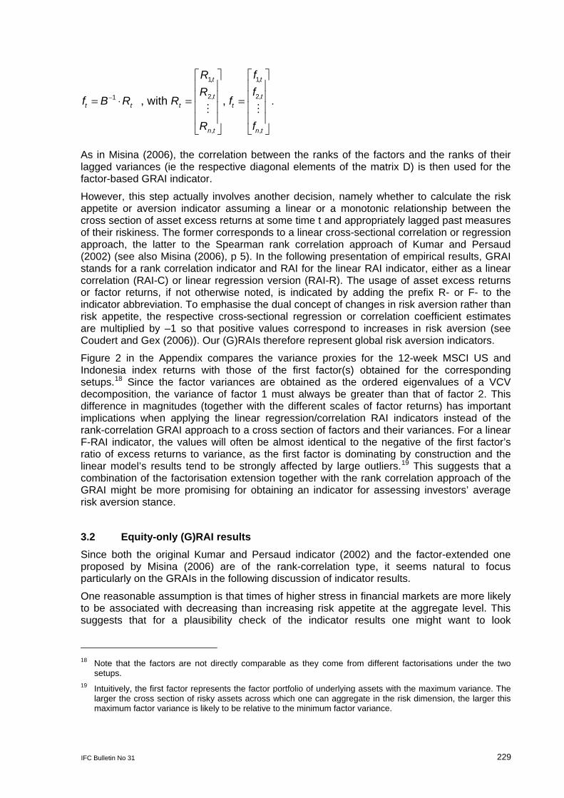
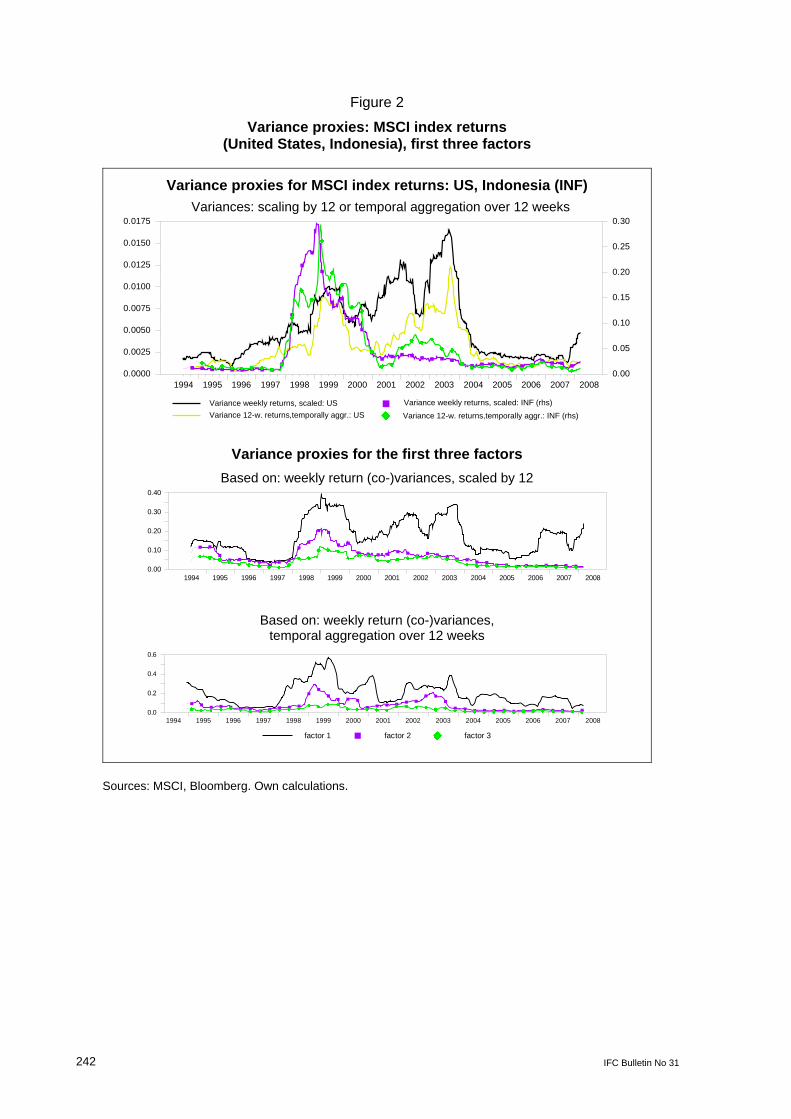
Figure 2 in the Appendix compares the variance proxies for the 12-week MSCI US and Indonesia index returns with those of the first factor(s) obtained for the corresponding setups.18 Since the factor variances are obtained as the ordered eigenvalues of a VCV decomposition, the variance of factor 1 must always be greater than that of factor 2. This difference in magnitudes (together with the different scales of factor returns) has important implications when applying the linear regression/correlation RAI indicators instead of the rank-correlation GRAI approach to a cross section of factors and their variances. For a linear F-RAI indicator, the values will often be almost identical to the negative of the first factor’s ratio of excess returns to variance, as the first factor is dominating by construction and the linear model’s results tend to be strongly affected by large outliers.19 This suggests that a combination of the factorisation extension together with the rank correlation approach of the GRAI might be more promising for obtaining an indicator for assessing investors’ average risk aversion stance.
3.2 Equity-only (G)RAI results Since both the original Kumar and Persaud indicator (2002) and the factor-extended one proposed by Misina (2006) are of the rank-correlation type, it seems natural to focus particularly on the GRAIs in the following discussion of indicator results.
One reasonable assumption is that times of higher stress in financial markets are more likely to be associated with decreasing than increasing risk appetite at the aggregate level. This suggests that for a plausibility check of the indicator results one might want to look
18 Note that the factors are not directly comparable as they come from different factorisations under the two
setups. 19 Intuitively, the first factor represents the factor portfolio of underlying assets with the maximum variance. The
larger the cross section of risky assets across which one can aggregate in the risk dimension, the larger this maximum factor variance is likely to be relative to the minimum factor variance.
230 IFC Bulletin No 31
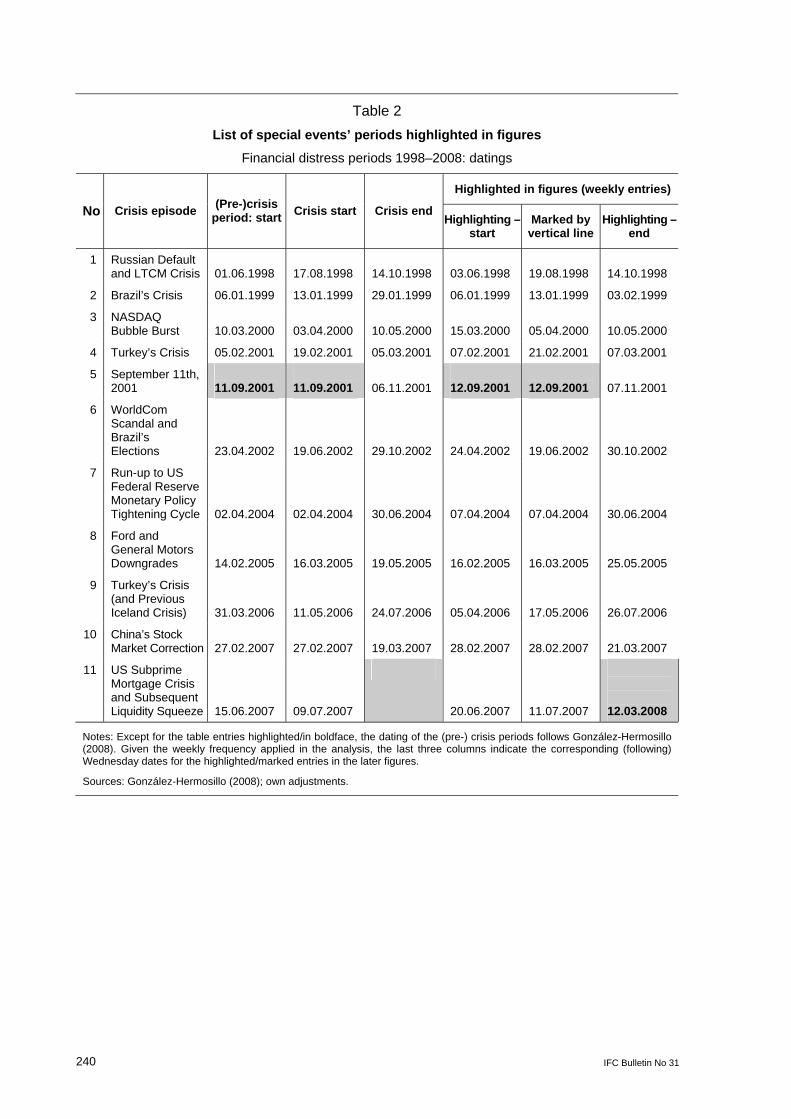
particularly at their behaviour during such periods. Some periods of likely higher financial market stress are therefore highlighted in the indicator graphs in the Appendix. The exact dating of these periods is given in Table 2 of the Appendix. For the most part it closely follows González-Hermosillo (2008). Apart from small adjustments due to the weekly frequency of the current analysis, in only two cases did it seem advisable to deviate from the choices made by González-Hermosillo (2008). The first deviation concerns the beginning of the stress episode following 11 September 2001, where for the purposes of this study the highlighted period starts on 12 September 2001.20 Furthermore, the end date for the US subprime mortgage crisis and ensuing liquidity squeeze episode was left open, since – as also noted by González-Hermosillo (2008) – the crisis was clearly still ongoing at the end of the sample period used for the following analysis (12 March 2008). Of course, the non-statistical method of dating these periods implies that there is a certain degree of discretion involved, particularly in terms of choosing the precrisis part of the highlighted periods.21 Furthermore, longer-term cyclical dynamics that overlay shorter-term dynamics in financial markets probably also contribute to the evolution of investors’ general risk appetite.
In addition, some of the figures in the Appendix also include horizontal lines corresponding to the critical values for a two-sided significance test of the rank correlation at a 5% significance level (for the critical values see Zar (1972)).
Overall, the graphs of the GRAI indicators for 12-week factor returns in Figure 3 of the Appendix appear more in line with priors concerning changes in risk appetite/aversion around critical periods than the results based on the original 12-week index returns. Despite the 12-week return periods, the GRAI patterns still retain a certain volatility. However, in all of the highlighted periods the F-GRAIs are either already in the positive domain or start to increase noticeably after the actual crisis event. At first sight, the crisis episode of the Ford and GM downgrades (no 8) appears to be different in this respect. The F-GRAIs drop immediately after 16 March 2005, the crisis event date given in González-Hermosillo (2008), when Moody’s announced their intention of reviewing GM’s credit rating. However, the crisis episode actually was played out over a protracted period and in different phases.22 In fact, the problems of Ford and GM already started to become more and more obvious in late 2004.23 The F-GRAIs seem better than the R-GRAIs at capturing this by moving from a significantly negative territory associated with still increasing risk appetite into a stance of eventually even increasing risk aversion. The initial increase is much more pronounced for the F-GRAI calculated from the lagged scaled VCV matrices of weekly returns than for the F-GRAI derived from temporally aggregated (co)variances of asset returns, however.24
20 González-Hermosillo (2008), on the other hand, chose a later date for her analysis, as some markets were
closed for a few days. 21 Alternatively, one may choose a more statistical approach of directly dating such crises. Coudert and Gex (2006)
used the CMAX indicator of Patel and Sarkar (1998) for dating stock market crises. 22 With the GM earnings warning of 16 March 2005 and the subsequent further ratings revisions the crisis in the
automotive sector reached another level. However, already on 14 October 2004, the losses from automotive sales in the United States and the resulting worsening of earnings prospects had made headlines, with the S&P rating for GM subsequently being lowered to the lowest investment-grade level. The crisis in the US automotive sector thus developed over a longer time. It reached another level of intensity when on 8 October 2005, the automotive parts company Delphi Corp., a former GM daughter, filed for Chapter 11 bankruptcy protection.
23 At the time the announcement for the review actually came, it might have not been such a shock for investors any more; their general risk appetite, although previously affected, might by that time have had a brief, temporary recovery.
24 However, in both cases the F-GRAIs still fall short of crossing the upper critical value bound. So even for the F-GRAI based on weekly return (co)variances, we cannot reject the null hypothesis of insignificance at the corresponding significance level (5% for a two-sided, 2.5% for a one-sided test)
IFC Bulletin No 31 231
One potential explanation of why the F-GRAIs might be more affected than the R-GRAIs by choosing to calculate the (co)variances as either a very short-term risk measure or a risk measure for a medium-term period could be that for the F-GRAIs this not only influences the risk rankings of assets. Due to the factorisation of the corresponding VCV matrices, it also has implications for the composition of the factors as portfolios of the underlying original assets. While the first factor is constructed to have a higher riskiness – ie variance – than the other factors, it will be constructed in the first case to exhibit the highest short-term riskiness of all factors. In the second case, however, it will rank higher than the remaining factors in terms of medium-term risk. Thus, for the F-GRAIs, the difference in the variance-covariance calculation translates into a different composition of the factors as derivative assets. This might produce a slightly less similar pattern for the F-GRAIs than for the R-GRAIs across the two methods of deriving riskiness proxies.25
While there is some similarity in the graphs of the indicators, the choice of factor returns instead of the original asset returns seems to have a clear impact on the results. One interesting period in this respect is early 1998, before the outbreak of the Russian crisis. Unlike the R-GRAIs, the F-GRAIs suggest at least a short period of significantly increasing risk appetite for early 1998, ie in the wake of the 1997 Asian financial crisis.26 Second, for the stock market downturn in 2002, the F-GRAIs – in contrast to the R-GRAIs – indicate significantly increasing risk aversion only at a later stage. This seems to fit in with the strongest stock market downturns occurring only in July and September of that year. Third, after the crisis of the Ford and GM downgrades, only the F-GRAIs give a clearer suggestion of actually declining risk appetite after 16 March 2005.
When comparing their overall patterns, the R-GRAIs appear at times more volatile and prone to very sharp corrections than the F-GRAIs. Before the Turkish crisis of 2006, the R-GRAIs still gave a strong indication that investors’ risk appetite was increasing. However, after the outbreak of the crisis the R-GRAIs again very significantly indicate a switch to increasing risk aversion. The F-GRAI changes take longer and are more muted, reaching a peak only towards the end of the highlighted period or even slightly later. Given the critical values, only for the F-GRAI based on temporally aggregated (co)variances is the implied increase in risk aversion weakly significant. But actually, regarding the timing of the increasing risk aversion as suggested by the F-GRAIs, one might also want to note another cause for concern around that time. Beginning in summer 2006, problems in the US housing market were mentioned more frequently.
This brings the discussion to the evolution of the indicators during the most recent crisis, the US subprime mortgage and liquidity crisis of 2007 and 2008.27 Given the level of stress observed in financial markets at that time, it seems strange that the equity-based R-GRAIs remain in the negative domain all through the summer of 2007, thus giving no indication of an increasing risk aversion around that time. The F-GRAIs, on the other hand, clearly suggest a decline of investor risk appetite after the outbreak of the crisis, and even point towards a significant increase in investors’ general risk aversion stance around August/September 2007. This initial increase of the F-GRAI is even more pronounced and longer-lasting when based on temporally aggregated (co)variances. In the latter case it was also matched by a stronger – and at the end of November/beginning of December 2007
25 For the period 5 January 2000 to 12 March 2008, the correlation between the 12-week GRAI indicators across
the two methods of calculating the (co)variances is approx 0.71 between the F-GRAIs and 0.93 between the R-GRAIs.
26 The R-GRAIs, on the other hand, remain in the positive domain, and as they are significant in early 1998, this suggests increasing risk aversion at that time.
27 A more detailed view of this period is given in the third panel of Figure 3, which covers only the year 2006 and later.
232 IFC Bulletin No 31
briefly significant – decline of risk aversion. However, early and mid-December 2007 brought a return to increasing risk aversion as far as the F-GRAIs are concerned. The R-GRAIs also suggest a change to increasing risk aversion, but in their case the change appears less pronounced. From February 2008 onwards, the R-GRAIs tentatively suggest an increasing risk appetite again, while the F-GRAIs lead us to conclude that investors’ risk aversion was still increasing overall. Looking at the end of the estimation period (mid-March 2008), it is possible only for the R-GRAI and the F-GRAI derived from temporally aggregated (co)variances to reject the hypothesis of zero rank correlation. However, while the F-GRAI would suggest significantly increasing risk aversion at that time, the R-GRAI suggests the opposite. In light of the markets’ worries about Bear Stearns during that period, this does not seem very likely. Considering the magnitude of the recent crisis, the results for the equity-only F-GRAIs are more in line with intuition. The modified Misina extension for the GRAI thus seems empirically useful, as it delivers more plausible results for the sample of international stock market indices.
Robustness of GRAI results to the choice of alternative return period lengths Figure 4 in the Appendix compares the GRAIs for 12-week returns with results obtained for four-week and 24-week returns in order to explore the sensitivity of results to the return period length.28 The results clearly show that the averaging effect of longer return periods has both benefits and downsides. When comparing results for 24-week with those for 12-week return periods, it seems that the downsides outweigh the benefits for 24-week returns. This is visible in the behaviour of the GRAI indicators not only during the latest crisis, but also to some extent after the 2006 crisis. While the 24-week return R-GRAIs at least suggest a significant increase of risk aversion sometime in the second half of 2006, the relatively long delay makes it somewhat difficult to see the direct connection to the crisis of 2006. Relative to the results for 24-week returns, the graphs of the four-week return period GRAI indicators appear more plausible. However, they are also more prone to strong corrections from time to time. The averaging effect of longer return periods implies that one loses potentially relevant information on short-term temporary effects on the stance of investors’ risk appetite changes. The GRAI indicators based on 12-week returns therefore reflect those changes only with a lag and/or in a much more muted fashion.
For the stress period starting in the summer of 2007, the results for a 12-week return period suggest a significant increase in investor risk aversion based on the F-GRAIs, but not for the R-GRAIs. For a four-week return period, the F-GRAIs suggest that investor risk aversion has started to increase even slightly earlier (already during June 2007). However, the change after the crisis event appears less pronounced than for the 12-week return F-GRAIs. The four-week return R-GRAIs, on the other hand, show a strong increase in indicator values after 7 July 2007. This indicates a shift to increasing risk aversion between early August and early September.29 But the significantly negative values of the four-week R-GRAIs from early September until around mid to late October 2007 suggests that the earlier period of increasing risk aversion was followed by a temporary correction period in which investor risk appetite started to increase again early on as well. Overall, the priors concerning the crisis effects on the confidence of investors are easier to reconcile with the graphs of the F-GRAIs than with the completely different scale of investor risk appetite recovery suggested by the four-week return R-GRAIs. The tendency of sharp corrections for four-week return GRAIs is
28 A corresponding six-month period was used in eg Wilmot, Mielczarski et al (2004) and Deutsche Bundesbank
(2005). However, a shorter period of one month instead of the preferred quarterly returns was also applied in Kumar and Persaud (2002), to demonstrate its effect on the indicator.
29 With the four-week return R-GRAIs even being above the critical value for a short period of time in between, which suggests a significant increase in risk aversion.
IFC Bulletin No 31 233
also very visible after the 2006 crisis. While suggesting a significant increase in risk aversion right after the outbreak of the crisis, the four-week R-GRAIs turn significantly negative even before the end of the highlighted stress period. Then, they temporarily shift back to being significantly positive again in September 2006. Balancing the trade-off between the information loss of longer and more volatile corrections with shorter return periods, 12-week return periods therefore appear to be a good compromise. In the following analyses they will be the preferred choice.
Comparison of GRAIs with (linear) RAI results (12-week return period length) If the relationship between excess returns and proxies for past riskiness is approximately linear and not only monotonic, the rank correlation results should be similar to those of a linear correlation approach (see also Misina (2006)). On the other hand, for a merely monotonic relationship the rank transformation should reduce the influence of extremes on estimating an aggregate or average relationship.
The first factor clearly is an extreme case, as by construction it will always have the highest historical variance within the set of given factors. One might therefore expect that the distinction between the rank and simple linear correlation approach should matter particularly for the results obtained when using the factor extension. This is also demonstrated in Figure 5 of the Appendix. The more pronounced amplitudes of the RAI-C indicators relative to the GRAIs suggest that the corresponding cross-sectional monotonic relationships exhibit some degree of non-linearity. This holds true even for the original asset returns. However, the difference in amplitudes – and thus the degree of the implied non-linearity – is much greater for the factor returns.
While the correlation-based indicators have the benefit of naturally bounded outcomes, the linear regression RAI-R indicators seem more popular in the literature. But as the factor extension exacerbates the non-linearity problem, it leads to the obvious question of the extent to which factor-based RAI-R results might be driven by the first factor. Figure 6 in the Appendix illustrates this problem. For the period of 2002–07, the graph of the RAI-R indicator using factor returns almost exactly overlaps the graph of the negative of the return/variance ratio for the first factor alone. Accordingly, the large t-values for the factor-based RAI-R indicators should be read as a further indication of the problem of applying a linear approach to a cross-section of such factors returns. However, Figure 6 also suggests that the indicator implied by the first factor alone might be another valuable risk appetite indicator – but with a different target group in mind. While the GRAI concentrates on the general or average risk appetite of investors overall, the risk appetite indicator implied by the first factor alone is concerned with the risk compensation for the derivative asset with highest risk. Thus, it may be regarded as informative concerning the risk appetite/aversion changes of a hypothetical marginal investor investing only in portfolios of the highest risk.
3.3 GRAIs – extending the coverage to bond market segments This section extends the coverage of financial market segments to bond markets, which are represented by a sample of Merrill Lynch bond and ABS indices (for details see Table 3 in the Appendix). Using a 12-week return period, Figure 7 compares the results for the GRAIs obtained for three data sets. For easier comparison, the results for the previous set of international stock indices are included as a first case (equity), in addition to the results for a second data set composed of corporate and ABS bond indices plus a US government bond index (bonds/USG). Finally, the two sets are merged into a third set of international stock and
234 IFC Bulletin No 31
bond indices (equity/bonds/USG). While Figure 7 covers the period from 2000 onwards, Figure 8 is a snapshot of the period starting in 2006.30
The graphs support the notion that investor risk appetite changes are sometimes different for the various market segments. However, the GRAIs for the merged set exhibit a greater degree of co-movement with the GRAIs derived from the stock indices alone than with the respective bond-only indicators.31 The highest degree of correspondence between the respective GRAIs for the merged and the bond set is obtained when using the factor extension combined with scaled one-week return VCV matrices.32 But as before, the choice of how to calculate the respective (co)variances has a greater overall impact on the F-GRAIs than on the R-GRAIs. This holds true for both the bonds-only and the merged data set.33
Focusing on the respective GRAI results before and during the latest financial stress period in Figure 8, one observes a strong increase of the bond-only R-GRAIs already in May 2007. Given the lack of a significant increase in the equity-set R-GRAIs around that time, this can be interpreted as risk aversion having increased in the bond market segment first. As this is the financial market segment immediately affected by the subprime mortgage crisis, this is plausible. However for equity and bond markets combined, the merged-set R-GRAI still suggests a significantly increasing risk appetite right up to 7 July 2007. After a short period of significantly increasing risk aversion around mid- to end of August 2007, it again implies a significantly increasing risk appetite at the merged-set level between October to mid-December 2007. However, considering the overall situation, the earlier increase and the later less significant reduction of the merged-set F-GRAI appear altogether more in line with common intuition. The differences are less pronounced when one takes into account that the significant risk aversion changes implied by the merged-set R-GRAIs were to some degree balanced by significant changes of opposite sign after the outbreak of the latest crisis period. Nevertheless, overall, the merged-set F-GRAIs are conservative in the sense that they less often suggest significant changes in investors’ risk appetite in the first place.
The choice of indices always involves some discretion. Due to its size and generally high degree of liquidity, the US government bond market plays a special role for international financial markets.34 The reference bond data set therefore includes only an index for the US Treasuries, but no government bond index for another major developed country. Hence Figure 9 in the Appendix compares the results obtained in the 2006–08 period for merged sets that differ slightly in terms of the government bond indices from developed countries
30 Apart from the highlighted periods of financial market stress, the figures also include the critical values for a
two-sided significance test of the rank correlation at a 5% significance level for a cross section of n = 46 (ie for the merged set of 24 international stock indices and 22 bond indices including the USG index). For the critical values see again Zar (1972).
31 For scaled VCVs and 12-week return periods eg the correlation between equity-only and merged-set F-GRAIs (R-GRAIs) in the period of 5 January 2000 to 12 March 2008, is roughly 0.72 (0.78) versus 0.55 (0.42) between bond-only and merged-set F-GRAIs (R-GRAIs).
32 For 12-week return periods, the correlation between the equity/bond/USG and bond/USG-only F-GRAIs (R-GRAIs) in the period of 5 January 2000 to 12 March 2008 is approx. 0.55 (0.42) under the scaling approach versus 0.28 (0.47) under the temporal aggregation approach to calculating VCVs.
33 The correlation between 12-week return period F-GRAIs (R-GRAIs) obtained with the two methods of calculating VCV matrices for the period of 5 January 2000 to 12 March 2008, is roughly 0.46 (0.98) for the bonds/USG set and 0.67 (almost 1) for the merged set.
34 US Treasuries are also often referred to as a kind of “safe haven” asset for international investors in stressful times.
IFC Bulletin No 31 235
they include.35 These small modifications, however, have only a negligible impact on the respective GRAI results.
3.4 A caveat – the GRAIs and the role of risk ranking stability Apart from the plausibility of results, an important criterion for judging indicators is the validity of core assumptions on which they are based. When constructing the GRAI for time t, it is conditional on the ranking of assets in terms of their return riskiness at the beginning of the m-week return period, ie at time t – m. Thus, one implicitly makes the simplifying assumption that this initial risk ranking of assets remains relevant to investors throughout the return period.36 However, investors may change their assessment of assets’ riskiness during the weeks of the return period, and the risk rankings of assets so most likely change as well. While the assumption is therefore likely to be violated to some extent, large violations obviously pose a problem. This holds true even if one is interested only in a broader risk appetite/aversion interpretation of the GRAI.37
One might expect this problem to grow with the length of the return period. Furthermore, the factor extension of the GRAI adds another dimension of complexity. This is particularly relevant for larger cross sections. Finally, whether the scaling or the temporal aggregation approach to calculating (co)variances is used can also matter. An analysis of the potential susceptibility of the different GRAI variants to great intraperiod changes in risk rankings is thus warranted. It also seems useful as a further criterion by which to judge their relative merits.
For the equity-only and combined-set F-/R-GRAIs, Figures 11–13 in the Appendix depict the maximum and minimum changes of (factor) asset variance ranks over the respective return period at each point in time, as well as the respective max-min spread. As expected, a longer return period is accompanied by larger max-min spreads of risk ranking changes. Furthermore, as illustrated by Figure 14, the method of obtaining VCV matrices via scaling overall produces smaller max-min spreads of (derivative) asset risk rank changes than the temporal aggregation approach. This holds true particularly for the F-GRAI, but generally also for the R-GRAI. Accordingly, for the equity-only data set, the F-GRAI has an advantage over the R-GRAI in terms of the risk ranking stability criterion, particularly when using scaled covariances and 12- and 24-week return periods. For the merged data set, the evidence of a risk ranking stability advantage of the F-GRAI over the R-GRAI is more mixed, as results depend on the combination of return period length and approach to calculating (co)variances. However, with respect to overall risk ranking stability, the combination of F-GRAI with scaled VCV matrices and longer return periods remains the preferred choice also for the merged equity-bond data set.38
35 Considering the combinations of USD valued government bond indices for the United States, United Kingdom
and Canada, plus, in a second step, also Germany, Australia and Japan; however, the case of including no government bond index is also considered.
36 Misina (2006) argued that any additional conclusion or interpretation of whether the GRAI might reflect changes in investors’ more narrowly defined fundamental degree of risk aversion was conditional on the likelihood of common shocks having occurred. As a proxy for the latter, he used the number of factors whose volatilities had changed in the same direction over the return period. The question of risk ranking stability considered here is of course related but still different, as it is concerned only with the question of the extent to which such changes of factor variances were so great as to have produced changes in (implied) risk rankings.
37 The greater the extent to which the assumption seems violated, the more problematic it becomes to interpret the signals of significant GRAI values as indicating at least changes of a broadly defined risk-aversion stance of investors.
38 Figure 15 in the Appendix also investigates whether a significant value of the GRAI coincides with a significant rank correlation between the asset/factor return variance changes over the return period and the past
236 IFC Bulletin No 31
3.5 A correlation-based comparison with alternative indicators The number of risk appetite indicators presented in the literature is ample evidence of the lack of consensus on how best to assess the evolution of investors’ risk appetite or the changes in the risk appetite. Nonetheless, assuming that the different indicators are all imperfect proxies for investors’ risk appetite/aversion changes, a principal component analysis (PCA) could be used to recover a potential common component as the common information contained in the individual indicators. However, when performing a PCA for nine market- and five theory-based risk appetite indicators, the ECB (2007b) found that the first two principal components together were able to explain only about 56% of the overall variance of the indicators. They therefore concluded that “differences in methodologies and underlying data” represented too big a problem when trying to recover “a common component between several commonly followed [market-based and theory-based] indicators”, which could “explain large proportions of their variance”. Accordingly, they derived their common component risk appetite indicator for the set of chosen market-based indicators alone.
It is thus important to understand better the extent to which these apparent differences between theory-based and market-based indicators depend on decisions made when constructing the indicators. Accordingly, not only GRAIs but also corresponding RAI variants are included in the following comparison with four alternative market-based risk sentiment indicators. We follow the ECB (2007b) and exploit the dimension-reducing properties of a PCA on the set of alternatives, however. Table 4 in the Appendix presents the correlation coefficients for each of the equity-only and merged-set (G)RAI variants and the first principal component of the four alternative market-based indicators, with values of 0.45 or greater highlighted.39 The results for the longer period of 8 November 2000 to 12 March 2008 can be summarised as follows:
• Comparing the correlation coefficients across the two methods of calculating the variance-covariance matrices, the differences are generally relatively small. The exception is the merged-set F-GRAI with 12-week return periods.
• Shortening return periods is usually accompanied by an increase in the correlation coefficients, all other things being equal. Market-based alternative indicators are likely to be relatively volatile given the continuous adjustments to changing market conditions. Hence, longer return periods might make it more difficult to capture this via the (G)RAI indicators, due to the implied smoothing effect. However, for the merged-set F-GRAI and the equity-only R-RAI-C, the choice of a 12-week return period resulted in higher correlation coefficients than either 24- or four-week return periods.
(ie beginning-of-period) variances. If there is a significant rank correlation between past variances and in-period variance changes with the same sign as the significant GRAI, one cannot exclude the possibility that the GRAI results might only reflect an adjustment of relative demand for riskier assets in response to the changes in the risk dimension, but not necessarily changes in the risk appetite/aversion stance of investors in a narrower sense. On the other hand, if the two are significant but opposite, this could tentatively be interpreted as a signal for increasing investor appetite for risk. The results in Figure 15 suggest that at times such interpretative problems could even be observed for the F-GRAIs. However, this is not the case at the beginning of the latest stress period, particularly when looking at equity markets, but also initially for the equity-bond data set. This further supports the notion that investor risk aversion itself increased during the initial stage.
39 The first principal component (explaining about 71% of the overall variance) was calculated for weekly (Wednesday) observations (from 1 April 1998 to 12 March 2008) of the following four indicators: the Citi Macro Risk Index (Bloomberg Ticker: MRI CITI Index), the risk aversion indicator implied by the Morgan Stanley Global Risk Demand Index (Ticker: STGRDI Index), the Westpac Risk Aversion Index (Ticker: WRAIRISK Index), and the UBS G10 Carry Risk Index Plus (ULTAFXRI Index). Where necessary, values were multiplied by –1 to correspond to a risk-aversion interpretation. Data for the original alternative indices were downloaded from Bloomberg.
IFC Bulletin No 31 237
• For the most part, the factor-extended (G)RAIs exhibit a higher correlation with the first principal component of the alternative indicators than the corresponding (G)RAIs without the factor extension. For the merged equity-bond data set, however, such a correlation advantage is obtained only for the 24-week return F-GRAI. The difference between the correlation coefficients obtained for the merged-set 12-week return F-GRAI based on scaled VCV matrices and for the corresponding merged-set R-GRAI is negligible, however.
The second panel of Table 4 explores the stability of results by focusing on the last five years of the sample period. The correlation coefficients obtained for the preferred combination of scaled VCV matrices and 12-week returns over this shorter recent period tend to be smaller. An exception is the corresponding merged-set F-GRAI. There we find an correlation advantage over the respective merged-set R-GRAI calculated with scaled (co)variances and 12-week returns. Overall, the correlation analysis therefore supports the conclusion that the gap between market-based and theory-based indicators can be considerably reduced when accounting for such specification effects in the construction of indicators. For the last few years in particular, the F-GRAIs obtained with the preferred setup of scaled VCV matrices and 12-week return periods are not only more appealing from a theoretical point of view. They also exhibit a higher degree of co-movement with the common component of the market-based risk aversion indicators than the corresponding R-GRAIs.
However, the greatest correlation coefficient across all GRAI variants is observed for the four-week return merged-set R-GRAI without the factor extension. This implies that a correlation analysis is illustrative but should not be a major criterion on which to base preferences concerning the specification of an indicator. The correlation between two series only measures their degree of co-movement. However, apart from the problem that aggregating across several alternative indicators still does not necessarily produce an ideal yardstick of investor risk appetite changes, other considerations are more important criteria, like the plausibility of results and underlying assumptions. As Figure 16 shows, during the latest crisis period the 12-week return equity-only and merged-set F-GRAIs delivered more plausible results and so seem preferable to the four-week return merged-set R-GRAI. The F-GRAIs are also more in line with the common component of the alternative market-based risk aversion indicators.
4. Summary and conclusions
Changes in investors’ risk appetite are increasingly being recognised as important factors in assessing financial markets stability. While this creates an obvious need for quantification, currently available risk appetite indicators are not satisfactory. Thus it is essential to gain a better understanding of how existing indicators actually work.
Focusing on the (G)RAI class of indicators, this study analyses how indicator results obtained for samples of stock indices, or stock and bond indices combined, are shaped by the various choices made when constructing such an indicator. Initial decisions include the choice of the length of return periods and how to proxy for the asset riskiness at the beginning of the return period. For the latter, we consider two options: using short-term asset risk measures based on scaling weekly return (co)variances, or longer-term risk measures derived via a temporal aggregation of weekly return (co)variances over a few weeks. One also has to decide whether to assume a monotonic or a linear relationship between asset excess returns and appropriately lagged risk measures when deriving the risk aversion indicator. Furthermore, one has to choose whether to derive it as a correlation- or regression-based indicator. The Kumar and Persaud (2002) GRAI indicator on which we focus is a rank-correlation indicator and thus based on the more general case of a monotonic relationship. Finally, another decision when constructing a GRAI concerns whether to account for a dependence between asset returns by applying a factor extension as proposed by
238 IFC Bulletin No 31
Misina (2006). Aside from analysing how all these decisions influence the final indicator produced, the main goal of this study is to find a combination of decisions that overall delivers the best empirical performance of the resulting risk aversion indicator in terms of certain plausibility and consistency criteria.
For comparability, Misina (2006) applied his indicator to an FX data set similar to that used by Kumar and Persaud (2002). One contribution of the current paper therefore consists of applying the factor-extended GRAI approach not only to individual financial market segments, but also to a large pooled data set covering equity and bond markets together. Furthermore, a spuriously different behaviour of GRAIs from their factor-extended versions can arise as a consequence of the normalisation of eigenvectors alone, unlike argued by Misina (2006), being insufficient for defining unique vectors. We therefore introduce a normalisation-plus restriction for the factorisation step to ensure the uniqueness of eigenvectors. This leads to our modified factor-extended rank-correlation F-GRAI as another major contribution of the present paper. Finally, we systematically investigate to what extent the factor extension in combination with the other construction choices leads to an improvement of the GRAIs’ empirical performance. Our most important guideline in this respect is the overall plausibility of the indicators with respect to the implied aggregate risk appetite changes during crisis times, in particular the recent period of financial market turmoil. However, another contribution of this paper is the development of additional consistency criteria for evaluating eg the relative attractiveness of F-GRAIs versus R-GRAIs. These criteria are based on violations of an important implicit assumption used in the construction of the GRAIs, namely intra-return period asset risk ranking stability.
Summing up the main empirical results, based on asset risk ranking stability considerations, we prefer the use of scaled VCV matrices when constructing the weekly GRAI indicators for the equity-only and the merged equity and bond data set. Furthermore, a return period length of 12 weeks appears to be a good compromise between the smoothness supplied by longer return periods and the loss of potentially important short-term information. Finally, for deriving an indicator for changes in average investor risk aversion, the GRAI rank-correlation approach seems preferable overall to the linear correlation or regression RAI variants. This holds particularly when the factor extension is applied. Focusing more narrowly on the GRAIs obtained for the preferred combination of 12-week returns and scaled (co)variances, we find in the equity-only case that the plausibility of results during the latest crisis benefits strongly from applying the rank correlation of Kumar and Persaud (2002) combined with our modified version of the Misina (2006) factor-transformation extension. For the larger cross section of the merged set of bond and stock indices, on the other hand, the GRAI without factor extension also indicates a significant increase in investor risk aversion, at least for some time in August 2007. However, although the larger cross section is likely to pose a challenge due to the additional complexity of the factorisation step, the merged-set factor-extended GRAI still fares quite well in terms of overall plausibility. Finally, over the period of March 2003 to March 2008, both the equity-only and the merged-set factor-extended GRAIs are also more closely correlated with the first principal component (PC) obtained for four market-based risk aversion indicators than the corresponding GRAIs without factor extension. This demonstrates the importance of taking into account indicator construction decisions as one way of potentially reducing the gap between market-based and theory-based indicators noted in ECB (2007b).
At the end of this paper, we have thus obtained two new feasible factor-extended GRAIs – one for stock markets alone, and one for stock and bond markets combined – which seem very promising for financial stability supervision purposes and future empirical applications. However, that is only one of this paper’s major achievements. Most importantly, we have gained a much better understanding of the chosen risk appetite indicator concept, and we have seen how strongly the quality of indicator results depends on technical implementation decisions. It is therefore absolutely essential to take this into account when using such indicators in practice.
IFC Bulletin No 31 239
Appendix
Table 1
MSCI stock indices USD
Name Ticker Abbreviation
MSCI USA MXUS Index US
MSCI Canada USD MSDUCA Index CA
MSCI Japan USD MSDUJN Index JN
MSCI UK USD MSDUUK Index UK
MSCI Germany USD MSDUGR Index GR
MSCI France USD MSDUFR Index FR
MSCI Ireland USD MSDUIE Index IE
MSCI Austria USD MSDUAT Index AT
MSCI Belgium USD MSDUBE Index BE
MSCI Netherlands USD MSDUNE Index NE
MSCI Italy USD MSDUIT Index IT
MSCI Spain USD MSDUSP Index SP
MSCI Finland USD MSDUFI Index FI
MSCI Norway USD MSDUNO Index NO
MSCI Sweden USD MSDUSW Index SW
MSCI Australia USD MSDUAS Index AS
MSCI New Zealand USD MSDUNZ Index NZ
MSCI Hong Kong USD MSDUHK Index HK
MSCI Emerging Markets Indonesia MSEUSINF Index INF
MSCI Malaysia USD MSDUMAF Index MAF
MSCI Emerging Markets Turkey MSEUSTK Index TK
MSCI Argentina MXAR Index AR
MSCI Brazil MXBR Index BR
MSCI Emerging Markets South Africa MSEUSSA Index SA
Sources: MSCI (Morgan Stanley Capital Intl.), Bloomberg.
240 IFC Bulletin No 31
Table 2
List of special events’ periods highlighted in figures
Financial distress periods 1998–2008: datings
Highlighted in figures (weekly entries)
No Crisis episode (Pre-)crisis period: start Crisis start Crisis end
Highlighting –start
Marked by vertical line
Highlighting –end
1 Russian Default and LTCM Crisis
01.06.1998
17.08.1998
14.10.1998
03.06.1998
19.08.1998
14.10.1998
2 Brazil’s Crisis 06.01.1999 13.01.1999 29.01.1999 06.01.1999 13.01.1999 03.02.1999
3 NASDAQ Bubble Burst
10.03.2000
03.04.2000
10.05.2000
15.03.2000
05.04.2000
10.05.2000
4 Turkey’s Crisis 05.02.2001 19.02.2001 05.03.2001 07.02.2001 21.02.2001 07.03.2001
5 September 11th, 2001
11.09.2001
11.09.2001
06.11.2001
12.09.2001
12.09.2001
07.11.2001
6 WorldCom Scandal and Brazil’s Elections
23.04.2002
19.06.2002
29.10.2002
24.04.2002
19.06.2002
30.10.2002
7 Run-up to US Federal Reserve Monetary Policy Tightening Cycle
02.04.2004
02.04.2004
30.06.2004
07.04.2004
07.04.2004
30.06.2004
8 Ford and General Motors Downgrades
14.02.2005
16.03.2005
19.05.2005
16.02.2005
16.03.2005
25.05.2005
9 Turkey’s Crisis (and Previous Iceland Crisis)
31.03.2006
11.05.2006
24.07.2006
05.04.2006
17.05.2006
26.07.2006
10 China’s Stock Market Correction
27.02.2007
27.02.2007
19.03.2007
28.02.2007
28.02.2007
21.03.2007
11 US Subprime Mortgage Crisis and Subsequent Liquidity Squeeze
15.06.2007
09.07.2007
20.06.2007
11.07.2007
12.03.2008
Notes: Except for the table entries highlighted/in boldface, the dating of the (pre-) crisis periods follows González-Hermosillo (2008). Given the weekly frequency applied in the analysis, the last three columns indicate the corresponding (following) Wednesday dates for the highlighted/marked entries in the later figures.
Sources: González-Hermosillo (2008); own adjustments.
IFC Bulletin No 31 241
Figure 1
Returns on MSCI index for the US: returns over 1, 4, and 12 weeks
Returns on MSCI index for the US
1-week returns 4-week returns 12-week returns
1993 1994 1995 1996 1997 1998 1999 2000 2001 2002 2003 2004 2005 2006 2007 2008-0.3
-0.2
-0.1
0.0
0.1
0.2
0.3
Sources: MSCI, Bloomberg. Own calculations.
242 IFC Bulletin No 31
Figure 2
Variance proxies: MSCI index returns (United States, Indonesia), first three factors
Variance proxies for MSCI index returns: US, Indonesia (INF)
Variances: scaling by 12 or temporal aggregation over 12 weeks
Variance w eekly returns, scaled: USVariance 12-w . returns,temporally aggr.: US
Variance w eekly returns: IND (rhs)Variance 12-w . returns,temporally aggr.: IND (rhs)
1994 1995 1996 1997 1998 1999 2000 2001 2002 2003 2004 2005 2006 2007 20080.0000
0.0025
0.0050
0.0075
0.0100
0.0125
0.0150
0.0175
0.00
0.05
0.10
0.15
0.20
0.25
0.30
Variance proxies for the first three factors Based on: weekly return (co-)variances, scaled by 12 y ( ) , y
1994 1995 1996 1997 1998 1999 2000 2001 2002 2003 2004 2005 2006 2007 20080.00
0.10
0.20
0.30
0.40
Based on: weekly return (co-)variances, temporal aggregation over 12 weeks y ( ) , p gg g
factor 1 factor 2 factor 3
1994 1995 1996 1997 1998 1999 2000 2001 2002 2003 2004 2005 2006 2007 20080.0
0.2
0.4
0.6
Sources: MSCI, Bloomberg. Own calculations.
Variance weekly returns, scaled: USVariance 12-w. returns,temporally aggr.: US
Variance weekly returns, scaled: INF (rhs) Variance 12-w. returns,temporally aggr.: INF (rhs)
Variances: scaling by 12 or temporal aggregation over 12 weeks
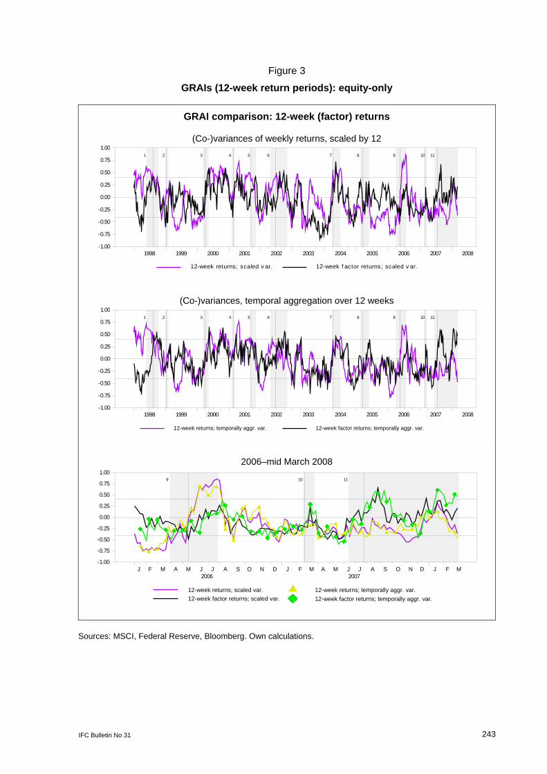
IFC Bulletin No 31 243
Figure 3
GRAIs (12-week return periods): equity-only
GRAI comparison: 12-week (factor) returns
(Co-)variances of weekly returns, scaled by 12
12-week returns; scaled v ar. 12-week f actor returns; scaled v ar.
1998 1999 2000 2001 2002 2003 2004 2005 2006 2007 2008-1.00
-0.75
-0.50
-0.25
0.00
0.25
0.50
0.75
1.001 2 3 4 5 6 7 8 9 10 11
(Co-)variances, temporal aggregation over 12 weeks
12-week returns; 12-week ret. v ar. 12-week f actor returns; 12-week ret. v ar.
1998 1999 2000 2001 2002 2003 2004 2005 2006 2007 2008-1.00
-0.75
-0.50
-0.25
0.00
0.25
0.50
0.75
1.001 2 3 4 5 6 7 8 9 10 11
2006–mid March 2008
12-week returns; scaled var.12-week factor returns; scaled var.
12-week returns; temporally aggr. var.12-week factor returns; temporally aggr. var.
J F M A M J J A S O N D J F M A M J J A S O N D J F M2006 2007
-1.00
-0.75
-0.50
-0.25
0.00
0.25
0.50
0.75
1.009 10 11
Sources: MSCI, Federal Reserve, Bloomberg. Own calculations.
12-week returns; scaled var. 12-week factor returns; scaled var.
12-week returns; temporally aggr. var. 12-week factor returns; temporally aggr. var.
12-week returns; temporally aggr. var. 12-week factor returns; temporally aggr. var.
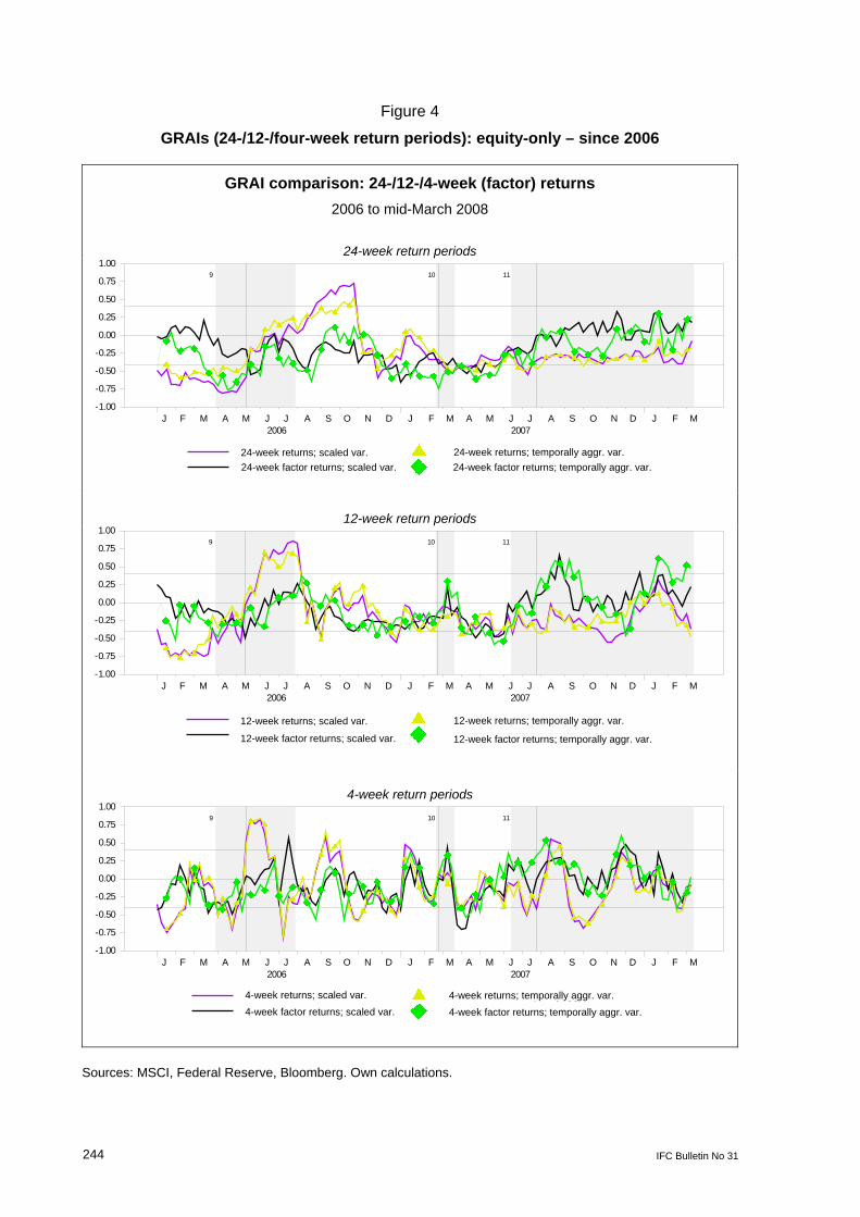
244 IFC Bulletin No 31
Figure 4
GRAIs (24-/12-/four-week return periods): equity-only – since 2006
GRAI comparison: 24-/12-/4-week (factor) returns 2006 to mid-March 2008
24-week return periods p
24-week returns; scaled var.24-week factor returns; scaled var.
24-week returns; temporally aggr. var.24-week factor returns; temporally aggr. var.
J F M A M J J A S O N D J F M A M J J A S O N D J F M2006 2007
-1.00
-0.75
-0.50
-0.25
0.00
0.25
0.50
0.75
1.009 10 11
12-week return periods
12-week returns; scaled var.12-week factor returns; scaled var.
12-week returns; temporally aggr. var.12-week factor returns; temporally aggr. var.
J F M A M J J A S O N D J F M A M J J A S O N D J F M2006 2007
-1.00
-0.75
-0.50
-0.25
0.00
0.25
0.50
0.75
1.009 10 11
4-week return periods p
4-week returns; scaled var.4-week factor returns; scaled var.
4-week returns; temporally aggr. var.4-week factor returns; temporally aggr. var.
J F M A M J J A S O N D J F M A M J J A S O N D J F M2006 2007
-1.00
-0.75
-0.50
-0.25
0.00
0.25
0.50
0.75
1.009 10 11
Sources: MSCI, Federal Reserve, Bloomberg. Own calculations.
24-week returns; scaled var. 24-week factor returns; scaled var.
12-week returns; scaled var.
12-week factor returns; scaled var.
4-week returns; scaled var. 4-week factor returns; scaled var.
24-week returns; temporally aggr. var. 24-week factor returns; temporally aggr. var.
12-week returns; temporally aggr. var.
12-week factor returns; temporally aggr. var.
4-week returns; temporally aggr. var. 4-week factor returns; temporally aggr. var.
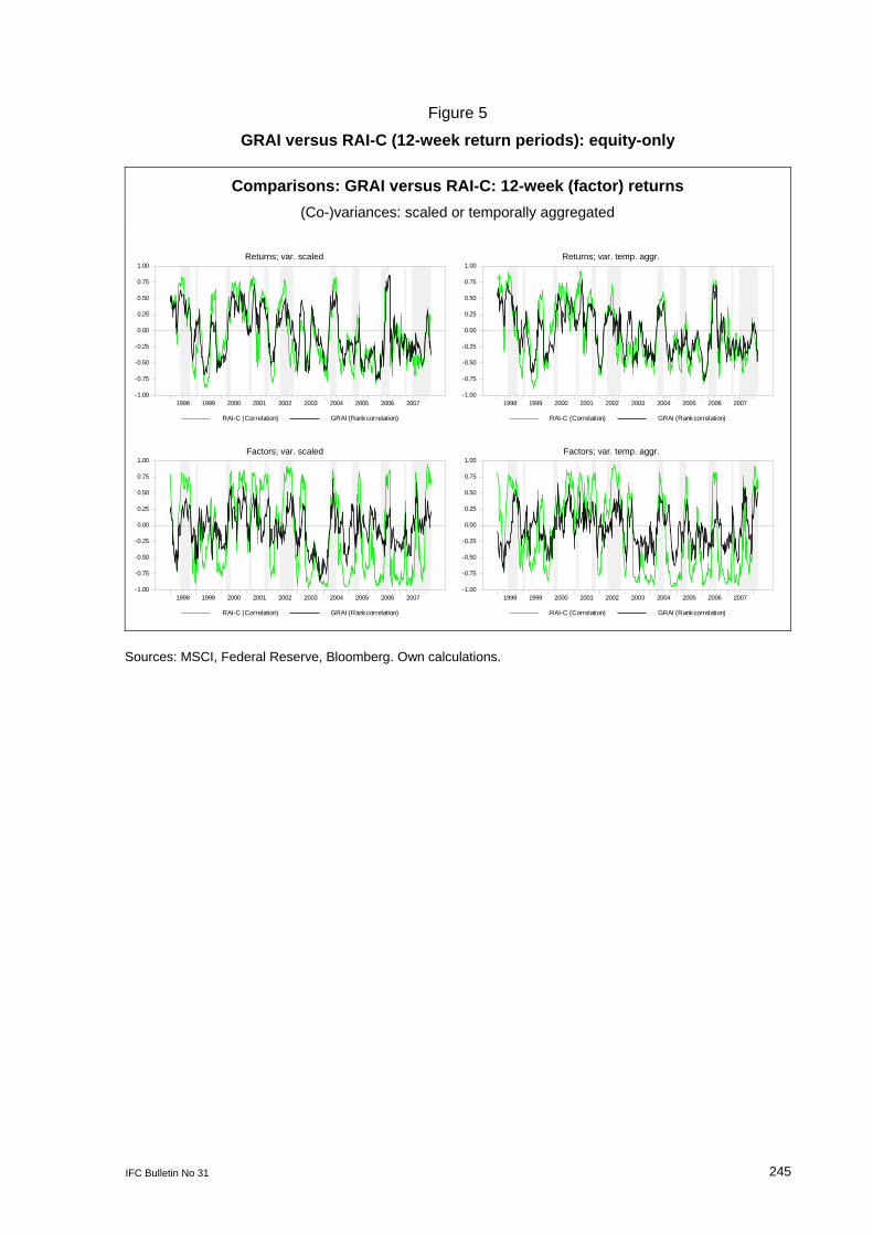
IFC Bulletin No 31 245
Figure 5
GRAI versus RAI-C (12-week return periods): equity-only
Comparisons: GRAI versus RAI-C: 12-week (factor) returns (Co-)variances: scaled or temporally aggregated
Returns; var.,scaled
RAI-C (Correlation) GRAI (Rank correlation)
1998 1999 2000 2001 2002 2003 2004 2005 2006 2007-1.00
-0.75
-0.50
-0.25
0.00
0.25
0.50
0.75
1.00
Factors; var.,scaled
RAI-C (Correlation) GRAI (Rank correlation)
1998 1999 2000 2001 2002 2003 2004 2005 2006 2007-1.00
-0.75
-0.50
-0.25
0.00
0.25
0.50
0.75
1.00
Returns; var.,temp.aggr.
RAI-C (Correlation) GRAI (Rank correlation)
1998 1999 2000 2001 2002 2003 2004 2005 2006 2007-1.00
-0.75
-0.50
-0.25
0.00
0.25
0.50
0.75
1.00
Factors; var.,temp.aggr.
RAI-C (Correlation) GRAI (Rank correlation)
1998 1999 2000 2001 2002 2003 2004 2005 2006 2007-1.00
-0.75
-0.50
-0.25
0.00
0.25
0.50
0.75
1.00
Sources: MSCI, Federal Reserve, Bloomberg. Own calculations.
Returns; var. scaled Returns; var. temp. aggr.
Factors; var. scaled Factors; var. temp. aggr.
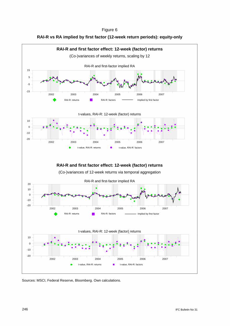
246 IFC Bulletin No 31
Figure 6
RAI-R vs RA implied by first factor (12-week return periods): equity-only
RAI-R and first factor effect: 12-week (factor) returns (Co-)variances of weekly returns, scaling by 12
RAI-R and first-factor implied RA
RAI-R: returns RAI-R: factors Implied by first factor
2002 2003 2004 2005 2006 2007-15
-5
5
15
t-values, RAI-R: 12-week (factor) returns
t-value, RAI-R: returns t-value, RAI-R: factors
2002 2003 2004 2005 2006 2007-20
-10
0
10
RAI-R and first factor effect: 12-week (factor) returns (Co-)variances of 12-week returns via temporal aggregation
RAI-R and first-factor implied RA
RAI-R: returns RAI-R: factors Implied by first factor
2002 2003 2004 2005 2006 2007-20
-10
0
10
20
t-values, RAI-R: 12-week (factor) returns ( )
t-value, RAI-R: returns t-value, RAI-R: factors
2002 2003 2004 2005 2006 2007-20
-10
0
10
Sources: MSCI, Federal Reserve, Bloomberg. Own calculations.
RAI-R: returns
t-value, RAI-R: returns
RAI-R: returns RAI-R: factors
RAI-R: factors
Implied by first factor
Implied by first factor
t-value, RAI-R: returns t-value, RAI-R: factors
t-value, RAI-R: factors
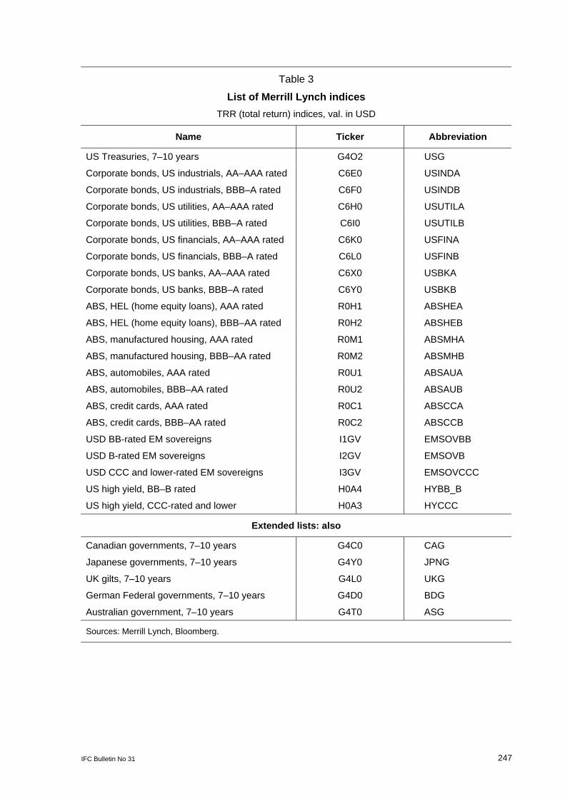
IFC Bulletin No 31 247
Table 3
List of Merrill Lynch indices TRR (total return) indices, val. in USD
Name Ticker Abbreviation
US Treasuries, 7–10 years G4O2 USG
Corporate bonds, US industrials, AA–AAA rated C6E0 USINDA
Corporate bonds, US industrials, BBB–A rated C6F0 USINDB
Corporate bonds, US utilities, AA–AAA rated C6H0 USUTILA
Corporate bonds, US utilities, BBB–A rated C6I0 USUTILB
Corporate bonds, US financials, AA–AAA rated C6K0 USFINA
Corporate bonds, US financials, BBB–A rated C6L0 USFINB
Corporate bonds, US banks, AA–AAA rated C6X0 USBKA
Corporate bonds, US banks, BBB–A rated C6Y0 USBKB
ABS, HEL (home equity loans), AAA rated R0H1 ABSHEA
ABS, HEL (home equity loans), BBB–AA rated R0H2 ABSHEB
ABS, manufactured housing, AAA rated R0M1 ABSMHA
ABS, manufactured housing, BBB–AA rated R0M2 ABSMHB
ABS, automobiles, AAA rated R0U1 ABSAUA
ABS, automobiles, BBB–AA rated R0U2 ABSAUB
ABS, credit cards, AAA rated R0C1 ABSCCA
ABS, credit cards, BBB–AA rated R0C2 ABSCCB
USD BB-rated EM sovereigns I1GV EMSOVBB
USD B-rated EM sovereigns I2GV EMSOVB
USD CCC and lower-rated EM sovereigns I3GV EMSOVCCC
US high yield, BB–B rated H0A4 HYBB_B
US high yield, CCC-rated and lower H0A3 HYCCC
Extended lists: also
Canadian governments, 7–10 years G4C0 CAG
Japanese governments, 7–10 years G4Y0 JPNG
UK gilts, 7–10 years G4L0 UKG
German Federal governments, 7–10 years G4D0 BDG
Australian government, 7–10 years G4T0 ASG
Sources: Merrill Lynch, Bloomberg.
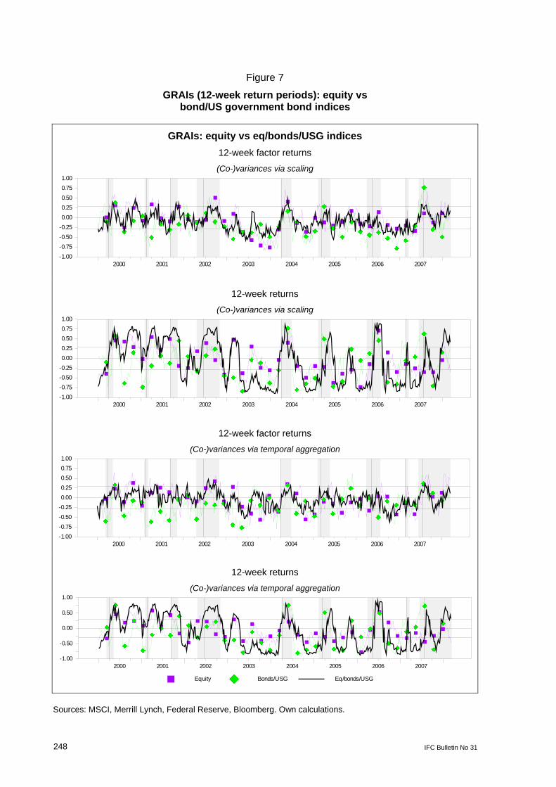
248 IFC Bulletin No 31
Figure 7
GRAIs (12-week return periods): equity vs bond/US government bond indices
GRAIs: equity vs eq/bonds/USG indices 12-week factor returns
(Co-)variances via scaling
2000 2001 2002 2003 2004 2005 2006 2007-1.00-0.75-0.50-0.250.000.250.500.751.00
12-week returns
(Co-)variances via scaling
2000 2001 2002 2003 2004 2005 2006 2007-1.00-0.75-0.50-0.250.000.250.500.751.00
12-week factor returns (Co-)variances via temporal aggregation
2000 2001 2002 2003 2004 2005 2006 2007-1.00-0.75-0.50-0.250.000.250.500.751.00
12-week returns
(Co-)variances via temporal aggregation
Equity Bonds/USG Eq/bonds/USG
2000 2001 2002 2003 2004 2005 2006 2007-1.00
-0.50
0.00
0.50
1.00
Sources: MSCI, Merrill Lynch, Federal Reserve, Bloomberg. Own calculations.
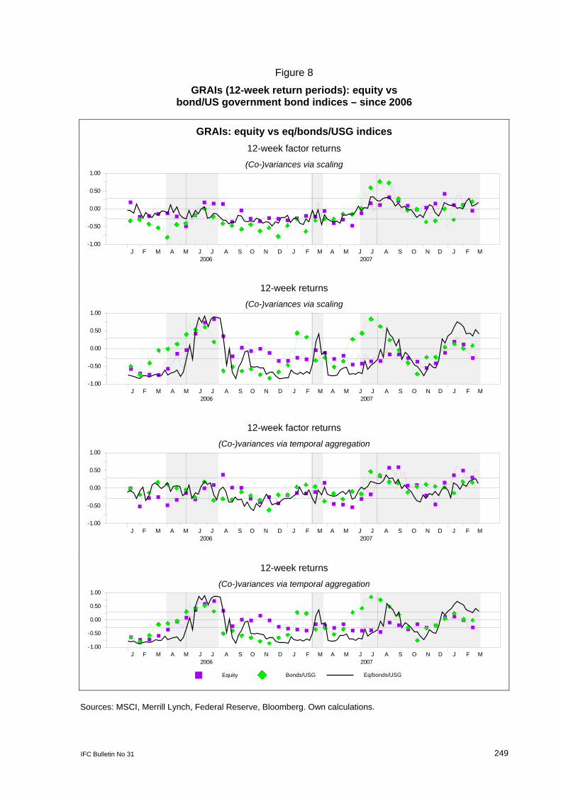
IFC Bulletin No 31 249
Figure 8
GRAIs (12-week return periods): equity vs bond/US government bond indices – since 2006
GRAIs: equity vs eq/bonds/USG indices 12-week factor returns
(Co-)variances via scaling
J F M A M J J A S O N D J F M A M J J A S O N D J F M2006 2007
-1.00
-0.50
0.00
0.50
1.00
12-week returns (Co-)variances via scaling
J F M A M J J A S O N D J F M A M J J A S O N D J F M2006 2007
-1.00
-0.50
0.00
0.50
1.00
12-week factor returns
(Co-)variances via temporal aggregation
J F M A M J J A S O N D J F M A M J J A S O N D J F M2006 2007
-1.00
-0.50
0.00
0.50
1.00
12-week returns
(Co-)variances via temporal aggregation
Equity Bonds/USG Eq/bonds/USG
J F M A M J J A S O N D J F M A M J J A S O N D J F M2006 2007
-1.00
-0.50
0.00
0.50
1.00
Sources: MSCI, Merrill Lynch, Federal Reserve, Bloomberg. Own calculations.
Eq/bonds/USG Bonds/USG Equity
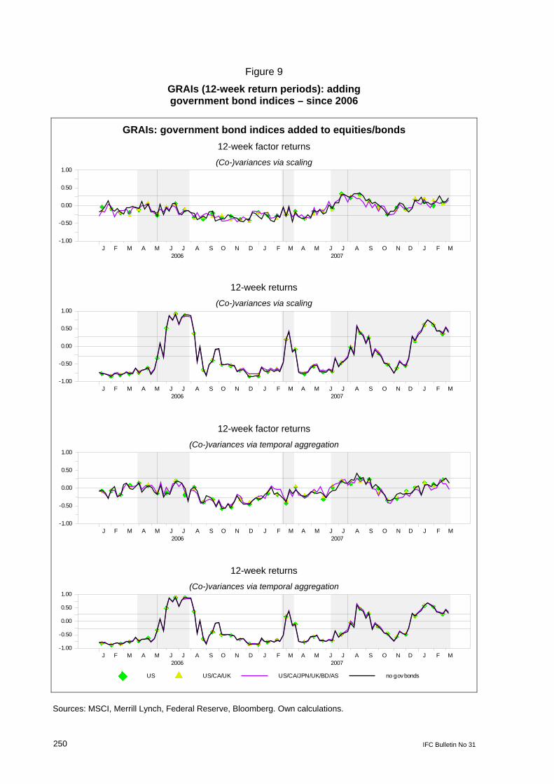
250 IFC Bulletin No 31
Figure 9
GRAIs (12-week return periods): adding government bond indices – since 2006
GRAIs: government bond indices added to equities/bonds 12-week factor returns
(Co-)variances via scaling
J F M A M J J A S O N D J F M A M J J A S O N D J F M2006 2007
-1.00
-0.50
0.00
0.50
1.00
12-week returns
(Co-)variances via scaling
J F M A M J J A S O N D J F M A M J J A S O N D J F M2006 2007
-1.00
-0.50
0.00
0.50
1.00
12-week factor returns
(Co-)variances via temporal aggregation
J F M A M J J A S O N D J F M A M J J A S O N D J F M2006 2007
-1.00
-0.50
0.00
0.50
1.00
12-week returns
(Co-)variances via temporal aggregation
US US/CA/UK US/CA/JPN/UK/BD/AS no gov bonds
J F M A M J J A S O N D J F M A M J J A S O N D J F M2006 2007
-1.00
-0.50
0.00
0.50
1.00
Sources: MSCI, Merrill Lynch, Federal Reserve, Bloomberg. Own calculations.
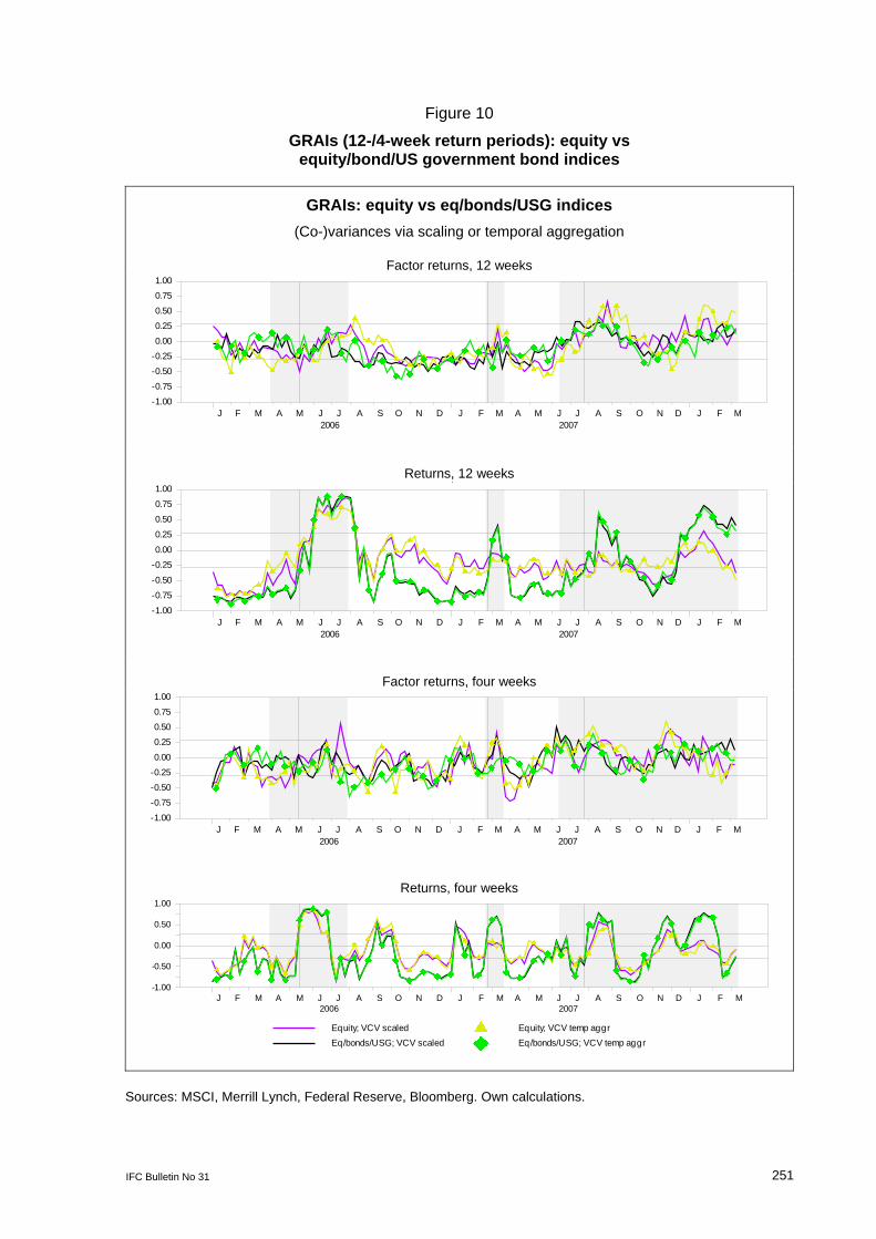
IFC Bulletin No 31 251
Figure 10
GRAIs (12-/4-week return periods): equity vs equity/bond/US government bond indices
GRAIs: equity vs eq/bonds/USG indices (Co-)variances via scaling or temporal aggregation
Factor returns, 12 weeks
J F M A M J J A S O N D J F M A M J J A S O N D J F M2006 2007
-1.00
-0.75-0.50-0.250.000.250.50
0.751.00
Returns, 12 weeks ,
J F M A M J J A S O N D J F M A M J J A S O N D J F M2006 2007
-1.00-0.75-0.50
-0.250.00
0.250.500.751.00
Factor returns, four weeks ,
J F M A M J J A S O N D J F M A M J J A S O N D J F M2006 2007
-1.00
-0.75-0.50-0.250.00
0.250.500.751.00
Returns, four weeks
Equity; VCV scaledEq/bonds/USG; VCV scaled
Equity; VCV temp aggrEq/bonds/USG; VCV temp aggr
J F M A M J J A S O N D J F M A M J J A S O N D J F M2006 2007
-1.00
-0.50
0.00
0.50
1.00
Sources: MSCI, Merrill Lynch, Federal Reserve, Bloomberg. Own calculations.
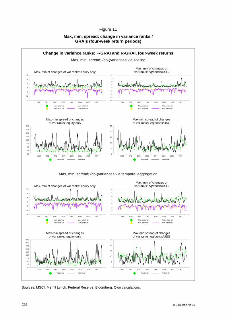
252 IFC Bulletin No 31
Figure 11
Max, min, spread: change in variance ranks / GRAIs (four-week return periods)
Change in variance ranks: F-GRAI and R-GRAI, four-week returns Max, min, spread; (co-)variances via scaling
Max, min of changes of var ranks: equity only Max, min of changes of
var ranks: eq/bonds/USG
Max, factor varMin, factor var
Max, return varMin, return var
2000 2001 2002 2003 2004 2005 2006 2007-15
-10
-5
0
5
10
15
Max, factor varMin, factor var
Max, return varMin, return var
2000 2001 2002 2003 2004 2005 2006 2007-20
-15
-10
-5
0
5
10
15
20
Max-min spread of changes of var ranks: equity only
Max-min spread of changes of var ranks: eq/bonds/USG
Factor var Return var
2000 2001 2002 2003 2004 2005 2006 20070.0
2.5
5.0
7.5
10.0
12.5
15.0
17.5
20.0
Factor var Return var
2000 2001 2002 2003 2004 2005 2006 20070
5
10
15
20
25
Max, min, spread; (co-)variances via temporal aggregation
Max, min of changes of var ranks: equity only Max, min of changes of
var ranks: eq/bonds/USG g y y
Max, factor varMin, factor var
Max, return varMin, return var
2000 2001 2002 2003 2004 2005 2006 2007-15
-10
-5
0
5
10
15g
Max, factor varMin, factor var
Max, return varMin, return var
2000 2001 2002 2003 2004 2005 2006 2007-15
-10
-5
0
5
10
15
20
Max-min spread of changes of var ranks: equity only
Max-min spread of changes of var ranks: eq/bonds/USG
Factor var Return var
2000 2001 2002 2003 2004 2005 2006 20070.0
2.5
5.0
7.5
10.0
12.5
15.0
17.5
20.0
22.5
Factor var Return var
2000 2001 2002 2003 2004 2005 2006 20070
5
10
15
20
25
Sources: MSCI, Merrill Lynch, Federal Reserve, Bloomberg. Own calculations.
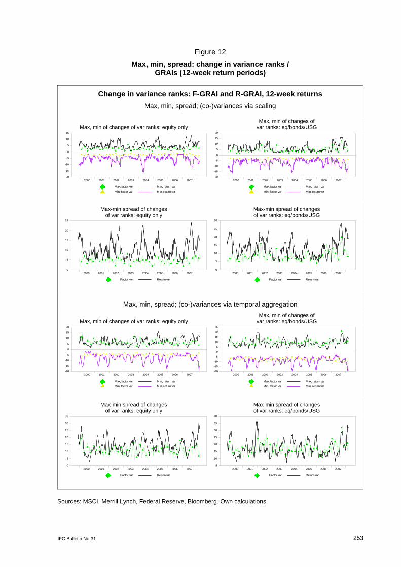
IFC Bulletin No 31 253
Figure 12
Max, min, spread: change in variance ranks / GRAIs (12-week return periods)
Change in variance ranks: F-GRAI and R-GRAI, 12-week returns Max, min, spread; (co-)variances via scaling
Max, min of changes of var ranks: equity only Max, min of changes of
var ranks: eq/bonds/USG
Max, factor varMin, factor var
Max, return varMin, return var
2000 2001 2002 2003 2004 2005 2006 2007-20
-15
-10
-5
0
5
10
15
Max, factor varMin, factor var
Max, return varMin, return var
2000 2001 2002 2003 2004 2005 2006 2007-20
-15
-10
-5
0
5
10
15
20
Max-min spread of changes of var ranks: equity only
Max-min spread of changes of var ranks: eq/bonds/USG
Factor var Return var
2000 2001 2002 2003 2004 2005 2006 20070
5
10
15
20
25
Factor var Return var
2000 2001 2002 2003 2004 2005 2006 20070
5
10
15
20
25
30
Max, min, spread; (co-)variances via temporal aggregation
Max, min of changes of var ranks: equity only Max, min of changes of
var ranks: eq/bonds/USG g y y
Max, factor varMin, factor var
Max, return varMin, return var
2000 2001 2002 2003 2004 2005 2006 2007-20
-15
-10
-5
0
5
10
15
20g
Max, factor varMin, factor var
Max, return varMin, return var
2000 2001 2002 2003 2004 2005 2006 2007-20
-15
-10
-5
0
5
10
15
20
25
Max-min spread of changes of var ranks: equity only
Max-min spread of changes of var ranks: eq/bonds/USG
Factor var Return var
2000 2001 2002 2003 2004 2005 2006 20070
5
10
15
20
25
30
35
Factor var Return var
2000 2001 2002 2003 2004 2005 2006 20075
10
15
20
25
30
35
40
Sources: MSCI, Merrill Lynch, Federal Reserve, Bloomberg. Own calculations.
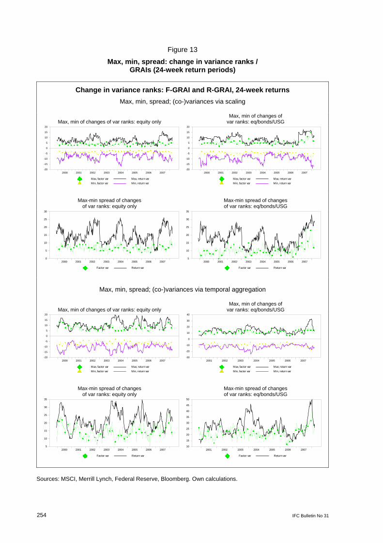
254 IFC Bulletin No 31
Figure 13
Max, min, spread: change in variance ranks / GRAIs (24-week return periods)
Change in variance ranks: F-GRAI and R-GRAI, 24-week returns Max, min, spread; (co-)variances via scaling
Max, min of changes of var ranks: equity only Max, min of changes of
var ranks: eq/bonds/USG
Max, factor varMin, factor var
Max, return varMin, return var
2000 2001 2002 2003 2004 2005 2006 2007-20
-15
-10
-5
0
5
10
15
20
Max, factor varMin, factor var
Max, return varMin, return var
2000 2001 2002 2003 2004 2005 2006 2007-20
-15
-10
-5
0
5
10
15
20
Max-min spread of changes of var ranks: equity only
Max-min spread of changes of var ranks: eq/bonds/USG
Factor var Return var
2000 2001 2002 2003 2004 2005 2006 20070
5
10
15
20
25
30
Factor var Return var
2000 2001 2002 2003 2004 2005 2006 20075
10
15
20
25
30
35
Max, min, spread; (co-)variances via temporal aggregation
Max, min of changes of var ranks: equity only Max, min of changes of
var ranks: eq/bonds/USG
Max, factor varMin, factor var
Max, return varMin, return var
2000 2001 2002 2003 2004 2005 2006 2007-20
-15
-10
-5
0
5
10
15
20
Max, factor varMin, factor var
Max, return varMin, return var
2001 2002 2003 2004 2005 2006 2007-30
-20
-10
0
10
20
30
40
Max-min spread of changes of var ranks: equity only
Max-min spread of changes of var ranks: eq/bonds/USG
Factor var Return var
2000 2001 2002 2003 2004 2005 2006 20075
10
15
20
25
30
35
Factor var Return var
2001 2002 2003 2004 2005 2006 200710
15
20
25
30
35
40
45
50
Sources: MSCI, Merrill Lynch, Federal Reserve, Bloomberg. Own calculations.
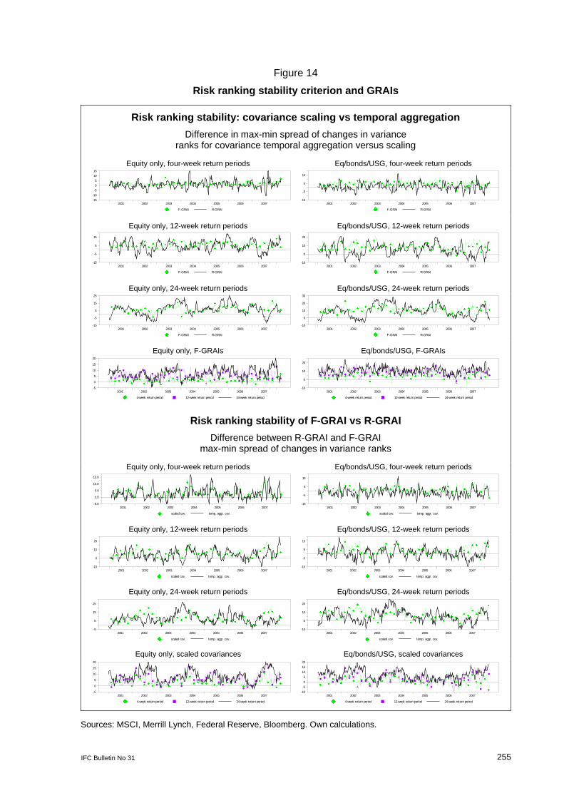
IFC Bulletin No 31 255
Figure 14
Risk ranking stability criterion and GRAIs
Risk ranking stability: covariance scaling vs temporal aggregation Difference in max-min spread of changes in variance
ranks for covariance temporal aggregation versus scaling
Equity only, four-week return periods Eq/bonds/USG, four-week return periods
F-GRAI R-GRAI
2001 2002 2003 2004 2005 2006 2007-15-10-505
1015
F-GRAI R-GRAI
2001 2002 2003 2004 2005 2006 2007-15
-5
5
15
Equity only, 12-week return periods Eq/bonds/USG, 12-week return periods
F-GRAI R-GRAI
2001 2002 2003 2004 2005 2006 2007-15
-5
5
15
F-GRAI R-GRAI
2001 2002 2003 2004 2005 2006 2007-10
0
10
20
Equity only, 24-week return periods Eq/bonds/USG, 24-week return periods
F-GRAI R-GRAI
2001 2002 2003 2004 2005 2006 2007-15
-5
5
15
25
F-GRAI R-GRAI
2001 2002 2003 2004 2005 2006 2007-10
0
10
20
30
Equity only, F-GRAIs Eq/bonds/USG, F-GRAIs
4-week return period 12-week return period 24-week return period
2001 2002 2003 2004 2005 2006 2007-5
0
5
10
15
20
4-week return period 12-week return period 24-week return period
2001 2002 2003 2004 2005 2006 2007-10
0
10
20
Risk ranking stability of F-GRAI vs R-GRAI Difference between R-GRAI and F-GRAI
max-min spread of changes in variance ranks
Equity only, four-week return periods Eq/bonds/USG, four-week return periods
scaled cov. temp. aggr. cov.
2001 2002 2003 2004 2005 2006 2007-5.0
0.0
5.0
10.0
15.0
scaled cov. temp. aggr. cov.
2001 2002 2003 2004 2005 2006 2007-15
-5
5
15
Equity only, 12-week return periods Eq/bonds/USG, 12-week return periods
scaled cov. temp. aggr. cov.
2001 2002 2003 2004 2005 2006 2007-10
0
10
20
scaled cov. temp. aggr. cov.
2001 2002 2003 2004 2005 2006 2007-15
-5
5
15
Equity only, 24-week return periods Eq/bonds/USG, 24-week return periods
scaled cov. temp. aggr. cov.
2001 2002 2003 2004 2005 2006 2007-5
5
15
25
scaled cov. temp. aggr. cov.
2001 2002 2003 2004 2005 2006 2007-10
0
10
20
Equity only, scaled covariances Eq/bonds/USG, scaled covariances y y
4-week return period 12-week return period 24-week return period
2001 2002 2003 2004 2005 2006 2007-5
0
5
10
15
20
4-week return period 12-week return period 24-week return period
2001 2002 2003 2004 2005 2006 2007-10-505
101520
Sources: MSCI, Merrill Lynch, Federal Reserve, Bloomberg. Own calculations.
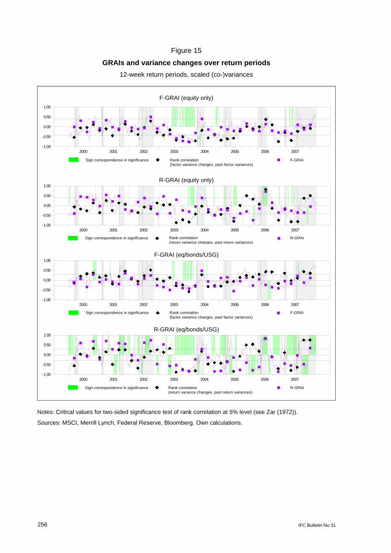
256 IFC Bulletin No 31
Figure 15
GRAIs and variance changes over return periods 12-week return periods, scaled (co-)variances
F-GRAI (equity only)
Sign correspondence in significance Rank correlation (factor var changes, past factor variances) F-GRAI
2000 2001 2002 2003 2004 2005 2006 2007-1.00
-0.50
0.00
0.50
1.00
R-GRAI (equity only) ( y y)
Sign correspondence in significance Rank correlation (return var changes, past return variances) R-GRAI
2000 2001 2002 2003 2004 2005 2006 2007-1.00
-0.50
0.00
0.50
1.00
F-GRAI (eq/bonds/USG)
Sign correspondence in significance Rank correlation (factor var changes, past factor variances) F-GRAI
2000 2001 2002 2003 2004 2005 2006 2007-1.00
-0.50
0.00
0.50
1.00
R-GRAI (eq/bonds/USG)
Sign correspondence in significance Rank correlation (return var changes, past return variances) R-GRAI
2000 2001 2002 2003 2004 2005 2006 2007-1.00
-0.50
0.00
0.50
1.00
Notes: Critical values for two-sided significance test of rank correlation at 5% level (see Zar (1972)).
Sources: MSCI, Merrill Lynch, Federal Reserve, Bloomberg. Own calculations.
Sign correspondence in significance
Sign correspondence in significance
Sign correspondence in significance
Sign correspondence in significance
Rank correlation (factor variance changes, past factor variances)
Rank correlation (return variance changes, past return variances)
Rank correlation (factor variance changes, past factor variances)
Rank correlation (return variance changes, past return variances)
F-GRAI
R-GRAI
F-GRAI
R-GRAI
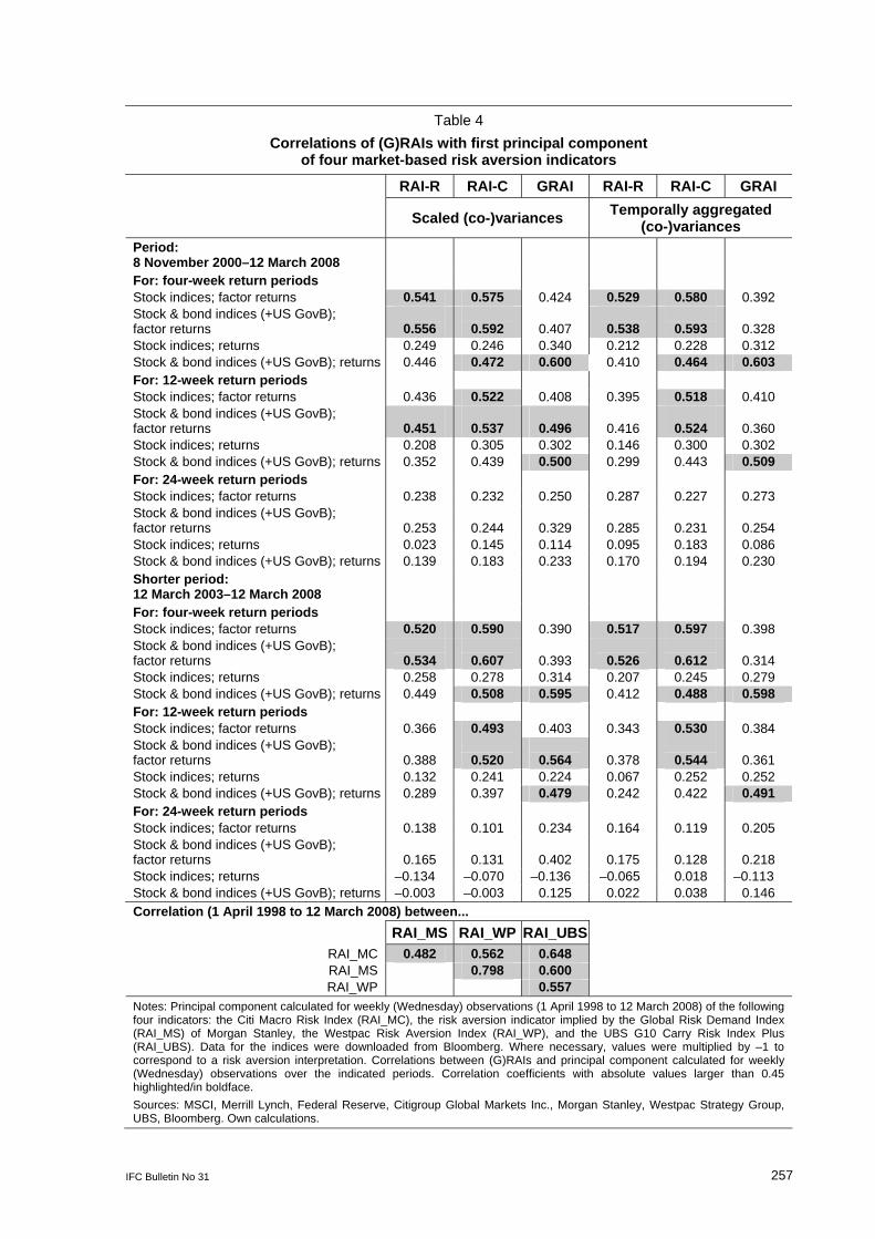
IFC Bulletin No 31 257
Table 4 Correlations of (G)RAIs with first principal component
of four market-based risk aversion indicators
RAI-R RAI-C GRAI RAI-R RAI-C GRAI
Scaled (co-)variances Temporally aggregated (co-)variances
Period: 8 November 2000–12 March 2008
For: four-week return periods Stock indices; factor returns 0.541 0.575 0.424 0.529 0.580 0.392 Stock & bond indices (+US GovB); factor returns
0.556
0.592
0.407
0.538
0.593
0.328
Stock indices; returns 0.249 0.246 0.340 0.212 0.228 0.312 Stock & bond indices (+US GovB); returns 0.446 0.472 0.600 0.410 0.464 0.603 For: 12-week return periods Stock indices; factor returns 0.436 0.522 0.408 0.395 0.518 0.410 Stock & bond indices (+US GovB); factor returns
0.451
0.537
0.496
0.416
0.524
0.360
Stock indices; returns 0.208 0.305 0.302 0.146 0.300 0.302 Stock & bond indices (+US GovB); returns 0.352 0.439 0.500 0.299 0.443 0.509 For: 24-week return periods Stock indices; factor returns 0.238 0.232 0.250 0.287 0.227 0.273 Stock & bond indices (+US GovB); factor returns
0.253
0.244
0.329
0.285
0.231
0.254
Stock indices; returns 0.023 0.145 0.114 0.095 0.183 0.086 Stock & bond indices (+US GovB); returns 0.139 0.183 0.233 0.170 0.194 0.230 Shorter period: 12 March 2003–12 March 2008
For: four-week return periods Stock indices; factor returns 0.520 0.590 0.390 0.517 0.597 0.398 Stock & bond indices (+US GovB); factor returns
0.534
0.607
0.393
0.526
0.612
0.314
Stock indices; returns 0.258 0.278 0.314 0.207 0.245 0.279 Stock & bond indices (+US GovB); returns 0.449 0.508 0.595 0.412 0.488 0.598 For: 12-week return periods Stock indices; factor returns 0.366 0.493 0.403 0.343 0.530 0.384 Stock & bond indices (+US GovB); factor returns
0.388
0.520
0.564
0.378
0.544
0.361
Stock indices; returns 0.132 0.241 0.224 0.067 0.252 0.252 Stock & bond indices (+US GovB); returns 0.289 0.397 0.479 0.242 0.422 0.491 For: 24-week return periods Stock indices; factor returns 0.138 0.101 0.234 0.164 0.119 0.205 Stock & bond indices (+US GovB); factor returns
0.165
0.131
0.402
0.175
0.128
0.218
Stock indices; returns –0.134 –0.070 –0.136 –0.065 0.018 –0.113 Stock & bond indices (+US GovB); returns –0.003 –0.003 0.125 0.022 0.038 0.146 Correlation (1 April 1998 to 12 March 2008) between...
RAI_MS RAI_WP RAI_UBS RAI_MC 0.482 0.562 0.648 RAI_MS 0.798 0.600 RAI_WP 0.557
Notes: Principal component calculated for weekly (Wednesday) observations (1 April 1998 to 12 March 2008) of the following four indicators: the Citi Macro Risk Index (RAI_MC), the risk aversion indicator implied by the Global Risk Demand Index (RAI_MS) of Morgan Stanley, the Westpac Risk Aversion Index (RAI_WP), and the UBS G10 Carry Risk Index Plus (RAI_UBS). Data for the indices were downloaded from Bloomberg. Where necessary, values were multiplied by –1 to correspond to a risk aversion interpretation. Correlations between (G)RAIs and principal component calculated for weekly (Wednesday) observations over the indicated periods. Correlation coefficients with absolute values larger than 0.45 highlighted/in boldface. Sources: MSCI, Merrill Lynch, Federal Reserve, Citigroup Global Markets Inc., Morgan Stanley, Westpac Strategy Group, UBS, Bloomberg. Own calculations.
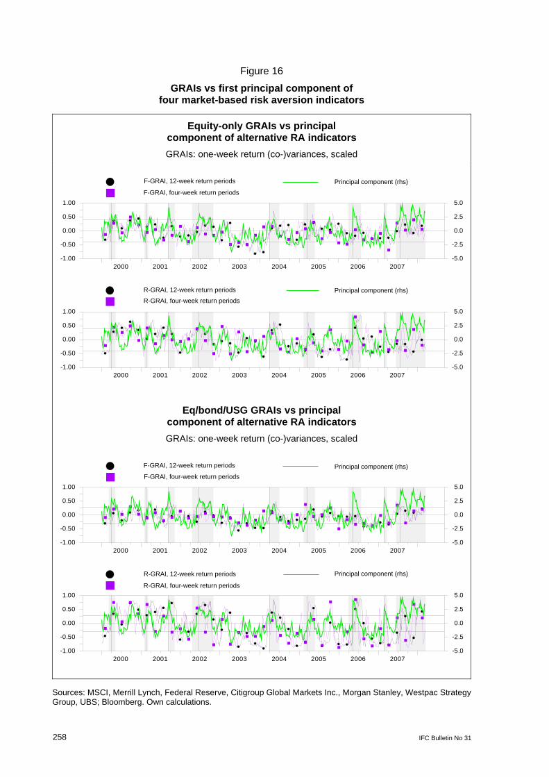
258 IFC Bulletin No 31
Figure 16
GRAIs vs first principal component of four market-based risk aversion indicators
Equity-only GRAIs vs principal component of alternative RA indicators GRAIs: one-week return (co-)variances, scaled
F-GRAI, 12-week return periodsF-GRAI, four-week return periods
Principal component (rhs)
2000 2001 2002 2003 2004 2005 2006 2007-1.00
-0.50
0.00
0.50
1.00
-5.0
-2.5
0.0
2.5
5.0
R-GRAI, 12-week return periodsR-GRAI, four-week return periods
Principal component (rhs)
2000 2001 2002 2003 2004 2005 2006 2007-1.00
-0.50
0.00
0.50
1.00
-5.0
-2.5
0.0
2.5
5.0
Eq/bond/USG GRAIs vs principal component of alternative RA indicators GRAIs: one-week return (co-)variances, scaled
F-GRAI, 12-week return periodsF-GRAI, four-week return periods
Principal component (rhs)
2000 2001 2002 2003 2004 2005 2006 2007-1.00
-0.50
0.00
0.50
1.00
-5.0
-2.5
0.0
2.5
5.0
R-GRAI, 12-week return periodsR-GRAI, four-week return periods
Principal component (rhs)
2000 2001 2002 2003 2004 2005 2006 2007-1.00
-0.50
0.00
0.50
1.00
-5.0
-2.5
0.0
2.5
5.0
Sources: MSCI, Merrill Lynch, Federal Reserve, Citigroup Global Markets Inc., Morgan Stanley, Westpac Strategy Group, UBS; Bloomberg. Own calculations.
F-GRAI, 12-week return periods
F-GRAI, four-week return periods Principal component (rhs)
Principal component (rhs) R-GRAI, 12-week return periods
R-GRAI, four-week return periods
F-GRAI, 12-week return periods
F-GRAI, four-week return periods
R-GRAI, 12-week return periods
R-GRAI, four-week return periods
Principal component (rhs)
Principal component (rhs)
IFC Bulletin No 31 259
References
Bollerslev, T, R F Engle and J M Wooldridge (1988): “A capital asset pricing model with time-varying covariances”, Journal of Political Economy, vol 96, no 1, pp 116–31.
Brandt, M W (2008): The econometrics of asset allocation: estimation error in asset allocation, Lecture Notes: Lecture no 2, Course at the Bank of Italy, 31 March–4 April.
Coudert, V and M Gex (2006): “Can risk aversion indicators anticipate financial crises?” Banque de France Financial Stability Review, no 9, December, pp 67–87.
Deutsche Bundesbank (2005): “Risk appetite in a dynamic financial market environment”, Deutsche Bundesbank Monthly Report, October, pp 85–97.
ECB (2007a): “Measuring financial market liquidity and risk aversion interdependence”, ECB Financial Stability Review, December, pp 176–81.
ECB (2007b): “Measuring investors’ risk appetite”, ECB Financial Stability Review, June, pp 166–71.
González-Hermosillo, B (2008): “Investors’ risk appetite and global financial market conditions”, IMF Working Paper WP/08/85, April.
Illing, M and M Aaron (2005): “A brief survey of risk-appetite indexes”, Bank of Canada Financial System Review, June, pp 37–43.
Kumar, M S and A Persaud (2002): “Pure contagion and investors’ shifting risk appetite: analytical issues and empirical evidence”, International Finance, vol 5, no 3, pp 401–36.
Misina, M (2003): “What does the risk-appetite index measure?” Bank of Canada Working Paper 2003-23, August.
Misina, M (2006): “Benchmark index of risk appetite”, Bank of Canada Working Paper 2006-16, May.
Patel, S and A Sarkar (1998): “Crises in developed and emerging stock markets”, Financial Analysts Journal, vol 54, no 6, November–December, pp 50–59.
Wilmot, J, P Mielczarski and J Sweeney (2004): “Global risk appetite index”, Credit Suisse First Boston, Global strategy research: Market focus, February.
Zar, J H (1972): “Significance testing of the Spearman rank correlation coefficient”, Journal of the American Statistical Association, vol 67, no 339, September, pp 578–80.