financial inclusion, rather than size, is the key to tackling income inequality

Working Paper n° 15/05 Madrid, February 2015

Financial inclusion, rather than size, is the key to tackling income inequality

Alicia García-Herrero

David Martínez Turégano

2 / 24 www.bbvaresearch.com

15/05 Working Paper

February 2015

Financial inclusion, rather than size, is the key to tackling income inequality* **

Alicia García-Herrero and David Martínez Turégano

Abstract

In this paper we assess empirically whether financial inclusion contributes to reducing income inequality

when controlling for other key factors, such as economic development and fiscal policy. We conclude that

financial inclusion contributes to reducing income inequality to a significant degree, while the size of the

financial sector does not. The policy implication of this result is that financial inclusion should be at the

forefront of government policies to reduce income inequality in a given economy. Given the broad way in

which we have defined inequality in our empirical analysis, this means facilitating the use of credit to both

households, especially low-income ones, as well as to small and medium-sized enterprises.

Keywords: income distribution, income inequality, Kuznets curve, financial development, financial deepening,

financial inclusion.

JEL: D63, F63, F65, G21, H23, O15.

*We thank Noelia Cámara for helpful comments and suggestions. **The views expressed are those of the authors and do not necessarily reflect those of BBVA Research or BBVA.


Working Paper

February 2015

1 Motivation

Income inequality has become a hot issue after years of irrelevance. In the developed world, the amazing

success of Thomas Piketty’s book1 in 2014 is clearly a good example. In the emerging world. unprecedented

reduction in poverty and a flourishing middle class co-exist with either more uneven income distributions –

like in India or China - or persistently high inequality – as in Latin America.

We could find one feasible explanation for these dynamics in a theory that proposes income inequality and

GDP per capita to relate in the form of an inverted U, or a so-called Kuznets curve2. In other words,

increasing inequality in countries in early stages of development would be no surprise when growth is high

and persistent, and workers are able to transition from low to medium or high productivity industries. This

was the case of Korea after the 50s and of China since the 90s. In the same way, we would expect that

countries in the middle income group would stabilise the degree of inequality, first, and then start to reduce it

as most of the workers enter the medium-high productivity industries and a welfare system starts being

introduced. This would be the case of several Latin American countries: Malaysia in Asia or Turkey in

Europe. Finally, the Kuznets curve anticipates a progressive reduction of income inequality for countries

reaching high-income levels. This was the case of Western economies from World War II until the 70s and

80s, when their welfare states continued to expand.

However, some developments point to shortcomings in the Kuznets theory. Among developed countries, the

income distribution seems to have worsened in many of them during the last few decades. In the same vein,

some emerging economies show significant deviations from the Kuznets curve when looking at the relation

between their GDP per capita and degree of inequality. To give two examples, this is the case of Vietnam or

Bangladesh.

Factors accounting for Kuznets-unexplained inequality could be either very persistent or founded on

historical reasons (e.g. through past land ownership or colonised conditions), or could be the result of

differentiated policies.

In this sense, the existing literature has devoted quite a lot of attention to the role of fiscal policies in taming

excessive inequality3, either through redistribution instruments (taxes and transfers), which mostly affect the

current income distribution, or in-kind policies (mainly education and health programmes), which have a

lagged impact on inequality, as relevant determinants of future income. Beyond this fiscal link, there is

growing interest in the impact of financial development on income inequality. In fact, one of the main

drawbacks faced by low-income individuals is the fact that they cannot smooth their income-savings path

due to the lack of access to financial instruments4. Access and use of credit should, thus, help to reduce

income inequality.

Financial development, as a concept, has been traditionally interpreted as financial deepening, which itself

has been proxied by the size of the financial system. In other words, for the same income per capita, a more

developed (i.e. larger) financial sector should be associated with a more evenly distributed income in a given

country.

While aware of the importance of financial constraints for the income of poorer households to grow, we

argue that a large financial system does not necessary coincide with easy access to and use of financial

services by those that are most financially constrained, namely households and especially lower-income

1: Piketty, Thomas, 2014, “Capital in the Twenty-First Century”, Harvard University Press. 2: Kuznets (1955). 3: See for example recent works by Journard, Pisu and Bloch (2014) and the IMF (2014). 4: Quadrini and Ríos-Rull (2014) includes a complete review of literature linking inequality and financial markets.


Working Paper

February 2015

ones, or Small and Medium Enterprises (SMEs) relative to large companies. In other words, we argue that

financial inclusion should be much more instrumental than financial deepening in reducing income inequality.

In this paper we assess empirically what role both dimensions of financial development (on the one hand the

size of the financial sector, and on the other access to and use of financial services) may have in reducing

income inequality. To that end, we show empirically that financial inclusion does contribute to reducing

income inequality while financial deepening does not when controlling for relevant factors, especially

economic development and fiscal policy.

The paper is distributed as follows. In Section 2 we review different measures for financial inclusion and

income distribution, underlining their advantages and disadvantages. In Section 3 we state our choices in

terms of variable definitions and proxies as well as the sources of our dataset and we also explain the

methodology used. In Section 4 some stylised facts are reviewed on the relation between financial inclusion

and income inequality. In Section 5 we show our results, and, finally, in Section 6 conclusions and

implications are drawn.


Working Paper

February 2015

2 Income inequality and financial inclusion:

measurement issues

Income inequality and financial inclusion are much harder to measure than more straight forward concepts in

economics. As for the former, the most common measure of income inequality is the GINI index, which is a

synthetic measure of how unevenly income is distributed among a ranked population. Other indicators only

capture a part of the distribution, such as the amount of income earned by a certain quantile or the ratio of

income per capita between different groups. Given its broader nature, we prefer to use the GINI coefficient

for our analysis.

Regardless of the preferred inequality measure, the main drawback when dealing with income distribution

data is heterogeneity across different countries (sometimes even across time). There are very few sources of

cross-country information on income distribution. One is the World Income Inequality Database (WIID) but –

unfortunately – countries report their information in very heterogeneous ways. In fact, they may use

consumption instead of income, or sometimes expenditure. Furthermore, when reporting income it may be

computed in gross or net terms (net standing for disposable income, namely after taxes and transfers).

Another disturbing issue is that the unit of analysis could be either the person or the household; in other

words the number of persons in the household may not be taken into account. Finally, and more generally,

the quality of the information differs across surveys5.

Unfortunately, due to the fact that income data are not collected on a continuous basis, there is usually a

strong trade-off between availability and homogeneity, the former being the predominant criterion in most

studies. In the same way, ours being a cross-country study, we need to choose the timeframe which

maximises the number of countries covered in our sample with the most homogenous data possible. With

that constraint in mind, cross-country GINI indices are most abundant after 2000, so that is our starting point

in time. We also filter the data by a number of criteria, to achieve as much homogeneity as possible.

The first one refers to the variable definition. We consider disposable income to be a more accurate measure

than gross income, particularly for those countries with a developed welfare state. Consumption or

expenditure could also fit with this idea, but surveys based on this concept are much less frequent and we

want to include emerging markets in our sample.

The second criterion is to use only surveys in which households are the statistical unit. Surveys covering

single individuals are usually limited to employees or taxpayers, excluding the rest and thus probably

underestimating inequality.

Finally, we include only data with full coverage on the area, population and age dimensions. Otherwise we

would be underestimating inequality, as we would expect people to be more homogeneous among certain

groups, such as urban or rural areas, young or older people.

Regarding the second concept of interest for this paper, financial inclusion, it is relatively recent and thus

quite difficult to define, let alone to measure. Sarma (2008) defines financial inclusion as “a process that

ensures the ease of access, availability and usage of the formal financial system for all members of an

economy”. In the same vein, Cámara and Tuesta (2014) define an inclusive financial system as “one that

maximises usage and access, while minimising involuntary financial exclusion”.

5: The WIID User Guide explains thoroughly the methodology and data issues of each income survey: http://bit.ly/1Ct7KN7

http://bit.ly/1Ct7KN7


Working Paper

February 2015

A number of surveys have been conducted6, trying to cover the different aspects of such definitions, but

samples are short in the time dimension, with most of the data starting after 2000. The lack of time series

calls for exploiting the cross-country differences in a cross-section analysis.

Based on the definitions above, and aware of the data constraints, we look for a set of variables which cover

at least one of the aspects previously mentioned. We look into both single variables on the households’ and

SMEs’ realms, but also into synthetic indicators of financial inclusion.

As a single indicator of households’ related financial inclusion, we take the percentage of adults with a bank

account, as provided by the World Bank and as compiled by Honohan (2007). As a single indicator of firms’

financial inclusion, and lacking data on loan distribution among companies, we take the amount of credit to

SMEs, either as a percentage of GDP or as a percentage of total outstanding loans from commercial banks.

Regarding more comprehensive – synthetic - indicators of financial inclusion, we use those developed so far

for a large enough group of countries. First of all, Sarma (2008) develops an index of financial inclusion

considering two dimensions; availability of banking services (bank branches per 1,000 population) and usage

(volume of credit and deposit as a %age of GDP). Second, Sarma (2008) also develops a three-dimension

indicator, namely adding the banking penetration dimension (number of bank accounts as a %age of total

population) to the previous two-dimension indicator. More recently Sarma (2012) compiles an index of

financial inclusion with one more variable, namely the number of Automatic Teller Machines (ATMs) per

100,000 inhabitants. In the same vein, Amidžić et al. (2014) offer a relatively similar four-variable index of

financial inclusion, namely the number of ATMs per 1,000 square kilometres, number of branches of Other

Depositary Corporations (ODCs) per 1,000 square kilometres, total number of resident household depositors

with ODCs per 1,000 adults and total number of resident household borrowers with ODCs per 1,000 adults.

Finally, Cámara and Tuesta (2014) compile an even more comprehensive index of financial inclusion

considering three dimensions: usage (percentage of adults holding an account, savings and loans), access

(ATMs and branches per capita and per area) and perceived barriers, which are not included in any other

index, such as distance to branches, affordability, documentation requirements and trust in the financial

system. Unfortunately, none of these synthetic indexes covers the financial inclusion of SMEs, so we will

need to use individual indicators as previously described.

6: Extensive and valuable information can be found in the Financial Access Survey (FAS) hosted by the IMF (http://fas.imf.org/), as well in the Global Findex Database (http://datatopics.worldbank.org/financialinclusion/) and the Global Financial Development Database (GFDD) (http://bit.ly/YhNr6n), both of them promoted by the World Bank.

http://fas.imf.org/

http://datatopics.worldbank.org/financialinclusion/

http://bit.ly/YhNr6n


Working Paper

February 2015

3 Our dataset and methodology

3.1 Data issues

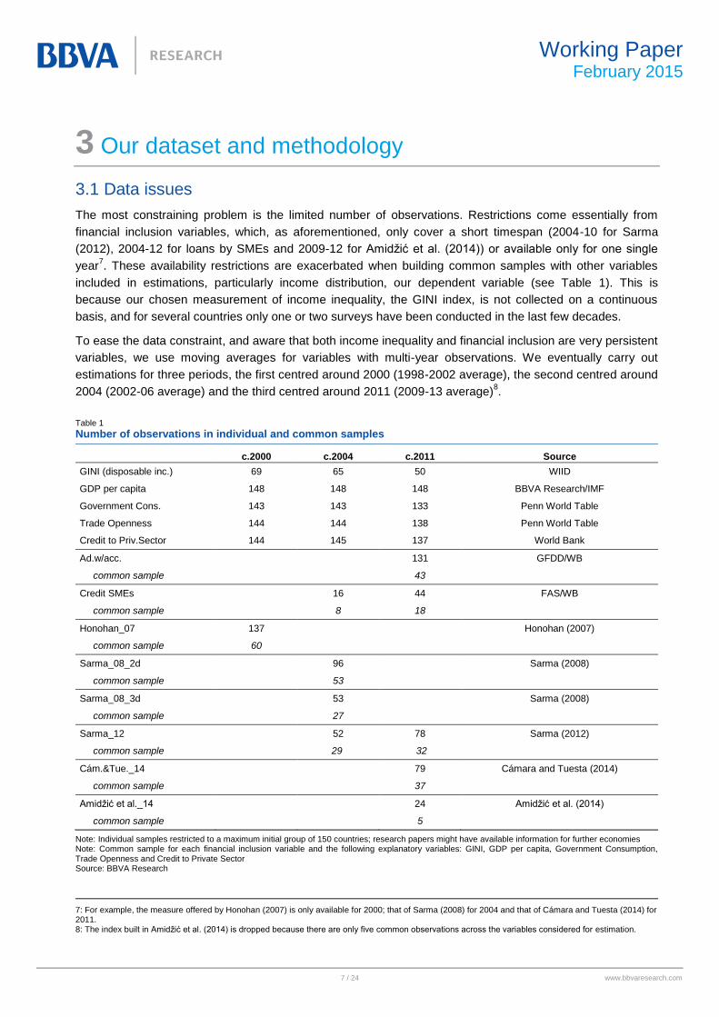
The most constraining problem is the limited number of observations. Restrictions come essentially from

financial inclusion variables, which, as aforementioned, only cover a short timespan (2004-10 for Sarma

(2012), 2004-12 for loans by SMEs and 2009-12 for Amidžić et al. (2014)) or available only for one single

year7. These availability restrictions are exacerbated when building common samples with other variables

included in estimations, particularly income distribution, our dependent variable (see Table 1). This is

because our chosen measurement of income inequality, the GINI index, is not collected on a continuous

basis, and for several countries only one or two surveys have been conducted in the last few decades.

To ease the data constraint, and aware that both income inequality and financial inclusion are very persistent

variables, we use moving averages for variables with multi-year observations. We eventually carry out

estimations for three periods, the first centred around 2000 (1998-2002 average), the second centred around

2004 (2002-06 average) and the third centred around 2011 (2009-13 average)8.

Table 1

Number of observations in individual and common samples

c.2000 c.2004 c.2011 Source

GINI (disposable inc.) 69 65 50 WIID

GDP per capita 148 148 148 BBVA Research/IMF

Government Cons. 143 143 133 Penn World Table

Trade Openness 144 144 138 Penn World Table

Credit to Priv.Sector 144 145 137 World Bank

Ad.w/acc.

131 GFDD/WB

common sample 43

Credit SMEs

16 44 FAS/WB

common sample 8 18

Honohan_07 137

Honohan (2007)

common sample 60

Sarma_08_2d

96

Sarma (2008)

common sample 53

Sarma_08_3d

53

Sarma (2008)

common sample 27

Sarma_12

52 78 Sarma (2012)

common sample 29 32

Cám.&Tue._14

79 Cámara and Tuesta (2014)

common sample 37

Amidžić et al._14

24 Amidžić et al. (2014)

common sample 5

Note: Individual samples restricted to a maximum initial group of 150 countries; research papers might have available information for further economies Note: Common sample for each financial inclusion variable and the following explanatory variables: GINI, GDP per capita, Government Consumption, Trade Openness and Credit to Private Sector Source: BBVA Research

7: For example, the measure offered by Honohan (2007) is only available for 2000; that of Sarma (2008) for 2004 and that of Cámara and Tuesta (2014) for 2011. 8: The index built in Amidžić et al. (2014) is dropped because there are only five common observations across the variables considered for estimation.


Working Paper

February 2015

Another problem we face is related to measurement errors in the dependent variable. In fact, as remarked in

Section 2, the GINI index is not a homogenous variable both for intra- and cross-country samples. There are

many methodological issues that make observations not fully comparable.

In order to reduce the heterogeneity of the dependent variable to the extent possible, we use only GINI

indexes based on disposable income with full coverage for the geographical area, age and population group

dimensions as defined in the WIID. Despite these filters, some sources of heterogeneity remain, such as the

survey quality or the accounting method for household composition but should not be large enough to affect

our conclusions.

3.2 Methodology Several variables could affect the income inequality, as measured by the GINI index. We, thus, would like to

control for them when estimating the impact of financial inclusion on income inequality. However, as the

sample is limited, we can only choose the most relevant ones.

As previously mentioned, the most important variable is obviously the fact that income per capita and income

inequality are expected to follow a Kuznets curve. We account for this by using the level and the square

value of the natural log of the GDP per capita (measured in real PPP-adjusted terms). The second widely

recognised determinant of income inequality is fiscal policy. To account for it, we include the ratio of

government consumption over GDP as a proxy for government size, and hence the fiscal power for

redistribution9. Finally, the degree of trade openness over GDP should capture the impact of external

developments in income distribution. While the literature is less unanimous on the direction of the sign of the

effect of openness on income distribution10

, our a priori is that trade – being welfare enhancing – should, in

principle, improve income inequality.

Finally, we do not only need to introduce measures of financial inclusion but also of financial size, to test our

hypothesis that the use of financial services may be more important that the actual size of the financial

sector. To that end, we measure size as bank credit to GDP.

Given data constraints, we can only run a two-period panel for single indicators of financial inclusion and a

simple cross-section for the synthetic indicators previously mentioned.

As for the estimation methodology, we face several problems.

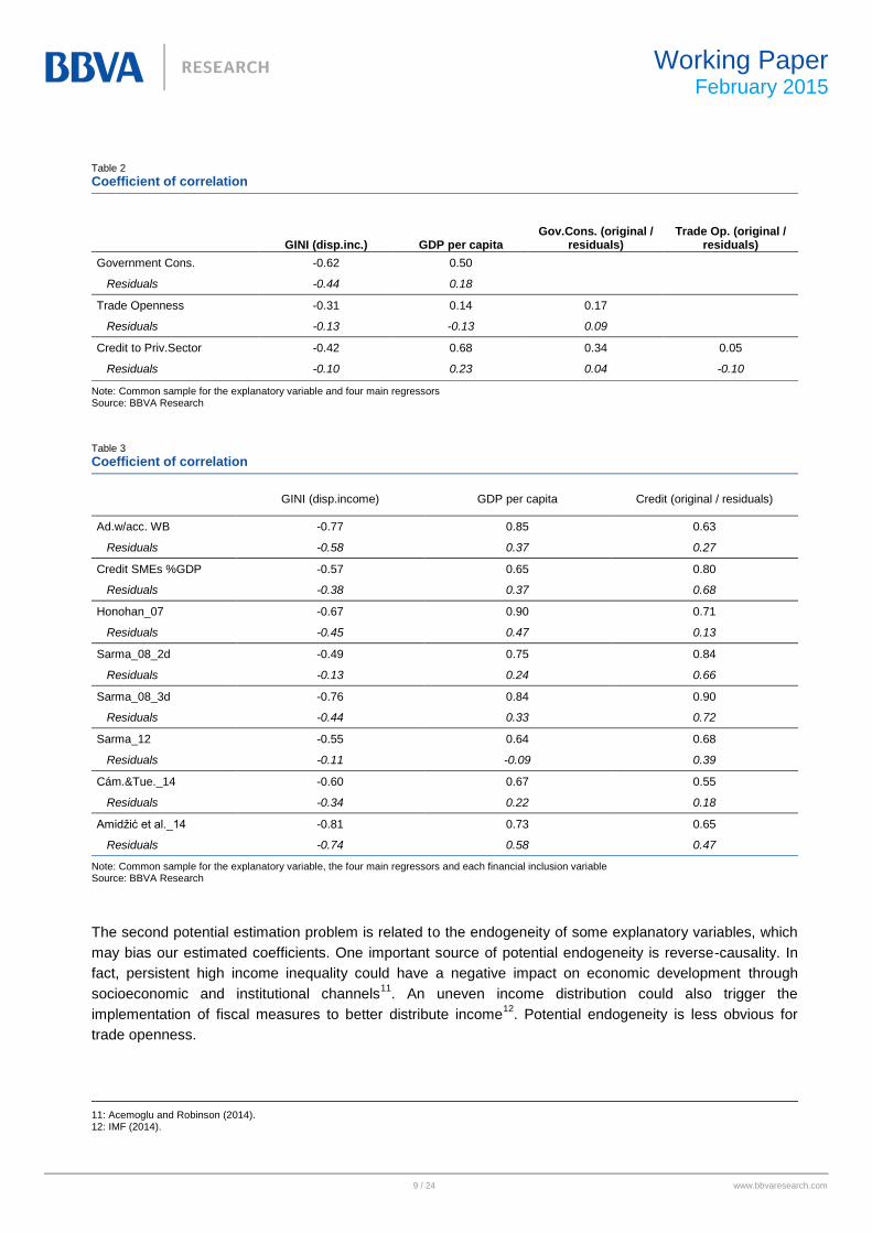
The first is collinearity between regressors, particularly between the GDP per capita and fiscal and financial

variables. As shown in Tables 2 and 3, collinearity between variables other than GDP per capita is

substantially reduced when we use residuals of a simple regression of these variables over GDP per capita.

The details on how to read our results under collinearity can be found in Section 5 below, with particular

focus on the distortion generated on variable contributions.

9: We prefer to use this measure rather than tax revenues since, as highlighted in IMF (2014), most of the redistribution is achieved through expenditure rather than revenue. 10: See for example Barro (2008) and Chakrabarti (2000).


Working Paper

February 2015

Table 2

Coefficient of correlation

GINI (disp.inc.) GDP per capita

Gov.Cons. (original / residuals)

Trade Op. (original / residuals)

Government Cons. -0.62 0.50

Residuals -0.44 0.18

Trade Openness -0.31 0.14 0.17

Residuals -0.13 -0.13 0.09

Credit to Priv.Sector -0.42 0.68 0.34 0.05

Residuals -0.10 0.23 0.04 -0.10

Note: Common sample for the explanatory variable and four main regressors Source: BBVA Research

Table 3

Coefficient of correlation

GINI (disp.income) GDP per capita Credit (original / residuals)

Ad.w/acc. WB -0.77 0.85 0.63

Residuals -0.58 0.37 0.27

Credit SMEs %GDP -0.57 0.65 0.80

Residuals -0.38 0.37 0.68

Honohan_07 -0.67 0.90 0.71

Residuals -0.45 0.47 0.13

Sarma_08_2d -0.49 0.75 0.84

Residuals -0.13 0.24 0.66

Sarma_08_3d -0.76 0.84 0.90

Residuals -0.44 0.33 0.72

Sarma_12 -0.55 0.64 0.68

Residuals -0.11 -0.09 0.39

Cám.&Tue._14 -0.60 0.67 0.55

Residuals -0.34 0.22 0.18

Amidžić et al._14 -0.81 0.73 0.65

Residuals -0.74 0.58 0.47

Note: Common sample for the explanatory variable, the four main regressors and each financial inclusion variable Source: BBVA Research

The second potential estimation problem is related to the endogeneity of some explanatory variables, which

may bias our estimated coefficients. One important source of potential endogeneity is reverse-causality. In

fact, persistent high income inequality could have a negative impact on economic development through

socioeconomic and institutional channels11

. An uneven income distribution could also trigger the

implementation of fiscal measures to better distribute income12

. Potential endogeneity is less obvious for

trade openness.

11: Acemoglu and Robinson (2014). 12: IMF (2014).


Working Paper

February 2015

For the variables of interest for this study, namely financial inclusion and size, Honohan (2007) points out

that such potential endogeneity is not likely to be as serious a problem when we try to explain income

inequality (or poverty, for that matter), as it would be if we were trying to explain income levels or growth13

.

Another source of potential endogeneity comes from common unobserved factors driving both the

dependent and the explanatory variables. This problem, however, should have been minimised in our

analysis, given robust control variables and lower correlations conditional on GDP per capita. Furthermore,

other studies on income inequality do not include a much larger set of regressors. In any case, potential

endogeneity issues as well as data limitations call for caution when interpreting our results.

Finally, another methodological challenge stems from the cross-country nature of our sample, which

introduces heteroskedasticity issues. We could expect variance of residuals to be different for countries with

diverse characteristics, for a number of reasons. The first is related to heterogeneity of the dependent

variable commented on in Section 2, and particularly to measurement errors: that we would expect them to

be higher in less-developed countries. Another source of heteroskedasticity would be the omission of

explanatory variables that asymmetrically affect different groups of countries. We analyse the potential

extent of these problems in Section 5.

13: This view is supported by other literature references which test the impact of different variables on income inequality and find no meaningful differences between OLS and GMM results. See for example Chakrabarti (2000) which focuses on the impact of trade openness on inequality or Gupta et al. (1998) on corruption and income inequality).


Working Paper

February 2015

4 Stylised facts

Before presenting the results of our estimations, we provide a quick overview on the relation between

financial inclusion – and financial size - with income inequality.

For this purpose, we first divide up the available observations of the GINI index according to the

development stage of each country: very low income (less than USD3,000 of GDP per capita), low income

(USD3,000-8,000), medium income (USD8,000-22,000) and high income (higher than USD22,000). We then

regress our key variables (financial inclusion and financial size) against the level and square values of GDP

per capita and split each sub-sample into those observations with significantly positive or negative residuals.

We conduct the same exercises for other control variables (Figure 1).

Figure 1

Average of GINI index for income groups and regressors conditioned on GDP per capita

Financial Inclusion Credit to GDP

Government Consumption to GDP

Trade Openness

Note: Regressors are Credit to Private Sector (% of GDP), Trade Openness (%GDP), Government Consumption (%GDP) and average for all financial inclusion variables Note: Values above average correspond to residuals of regressions on GDP per capita (level and square values) that are one standard deviation above mean (0) Source: BBVA Research

0

10

20

30

40

50

60

Very lowincome

Low Income MediumIncome

High Income

Average FinInc>Avg FinInc<Avg

0

10

20

30

40

50

60

Very lowincome


High Income

Average CreditGDP>Avg CreditGDP<Avg

0

10

20

30

40

50

60

Very lowincome


High Income

Average GovCons>Avg GovCons<Avg

0

10

20

30

40

50

60

Very lowincome


High Income

Average TradeOp>Avg TradeOp<Avg


Working Paper

February 2015

Interestingly, we find that - relative to the estimated expected values conditioned on GDP per capita - higher

income inequality is generally associated with less financial inclusion but more financial size. In the same

vein, and as one would expect, a more unequal income distribution is associated with lower fiscal

redistribution proxied by government consumption. According to the figures, this variable would have the

larger incidence on inequality, particularly for low- and medium-income countries. Finally, trade openness

shows in our analysis a negative association with inequality when controlling for economic development. In

other words, a more open economy – other things being given – tends to experience lower income

inequality.

In a second analysis, we now divide the observations according both to the IMF classification between

developed and emerging countries and, among the latter, to the geographical location of the countries

(Eastern Europe, Asia, Latin America and Africa).

Results are in this case less conclusive as when dividing by income per capita (Figure 2). In general terms,

dispersion within group is lower, suggesting geographical common drivers of inequality, as we will highlight

in the next section.

Figure 2

Average of GINI index for regions and regressors conditioned on GDP per capita

Financial Inclusion Credit to GDP

Government Consumption to GDP Trade Openness

Note: Regressors are Credit to Private Sector (% of GDP), Trade Openness (%GDP), Government Consumption (%GDP) and average for all financial inclusion variables Note: Values above average correspond to residuals of regressions on GDP per capita (level and square values) that are one standard deviation above mean (0) Source: BBVA Research

0

10

20

30

40

50

60

70

Develo

p.

E.E

uro

pe

Em

g.A

sia

L.A

merica

Afr

ica

Average FinInc>Avg FinInc<Avg

0

10

20

30

40

50

60

70D

evelo

p.

E.E

uro

pe

Em

g.A

sia

L.A

me

rica

Afr

ica

Average CreditGDP>Avg CreditGDP<Avg

0

10

20

30

40

50

60

70

Develo

p.

E.E

uro

pe

Em

g.A

sia

L.A

merica

Afr

ica

Average GovCons>Avg GovCons<Avg

0

10

20

30

40

50

60

Develo

p.

E.E

uro

pe

Em

g.A

sia

L.A

me

rica

Afr

ica

Average TradeOp>Avg TradeOp<Avg


Working Paper

February 2015

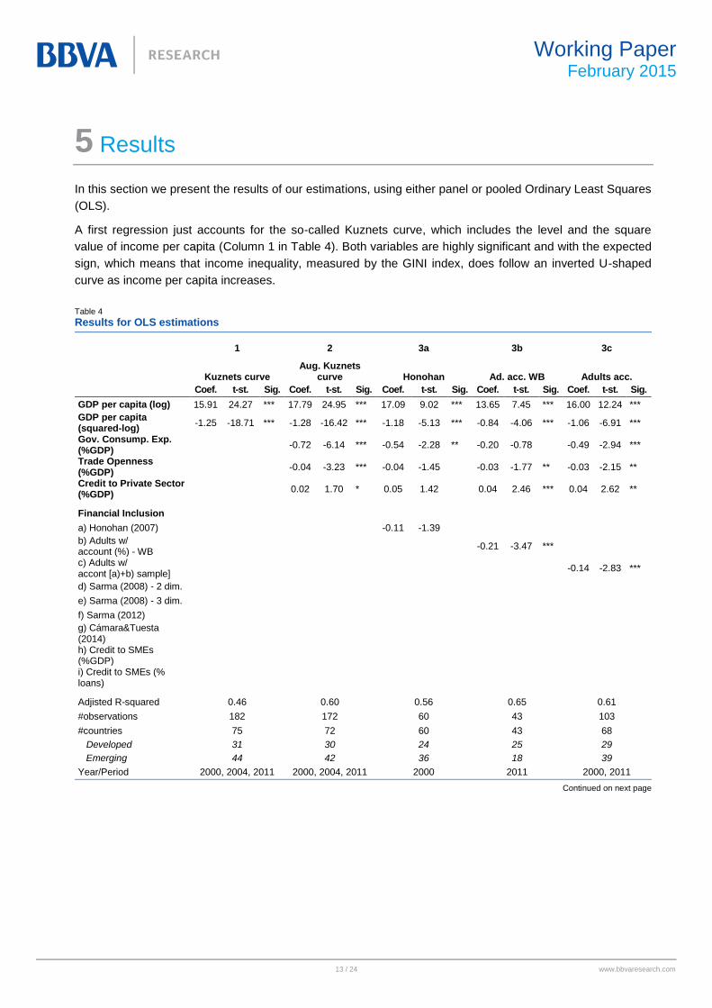
5 Results

In this section we present the results of our estimations, using either panel or pooled Ordinary Least Squares

(OLS).

A first regression just accounts for the so-called Kuznets curve, which includes the level and the square

value of income per capita (Column 1 in Table 4). Both variables are highly significant and with the expected

sign, which means that income inequality, measured by the GINI index, does follow an inverted U-shaped

curve as income per capita increases.

Table 4

Results for OLS estimations

1 2 3a 3b 3c

Kuznets curve Aug. Kuznets

curve Honohan Ad. acc. WB Adults acc.

Coef. t-st. Sig. Coef. t-st. Sig. Coef. t-st. Sig. Coef. t-st. Sig. Coef. t-st. Sig.

GDP per capita (log) 15.91 24.27 *** 17.79 24.95 *** 17.09 9.02 *** 13.65 7.45 *** 16.00 12.24 ***

GDP per capita (squared-log)

-1.25 -18.71 *** -1.28 -16.42 *** -1.18 -5.13 *** -0.84 -4.06 *** -1.06 -6.91 ***

Gov. Consump. Exp. (%GDP)

-0.72 -6.14 *** -0.54 -2.28 ** -0.20 -0.78

-0.49 -2.94 ***

Trade Openness (%GDP)

-0.04 -3.23 *** -0.04 -1.45

-0.03 -1.77 ** -0.03 -2.15 **

Credit to Private Sector (%GDP)

0.02 1.70 * 0.05 1.42

0.04 2.46 *** 0.04 2.62 **

Financial Inclusion

a) Honohan (2007)

-0.11 -1.39

b) Adults w/ account (%) - WB

-0.21 -3.47 ***

c) Adults w/ accont [a)+b) sample]

-0.14 -2.83 ***

d) Sarma (2008) - 2 dim.

e) Sarma (2008) - 3 dim.

f) Sarma (2012)

g) Cámara&Tuesta (2014) h) Credit to SMEs (%GDP) i) Credit to SMEs (% loans)

Adjisted R-squared 0.46 0.60 0.56 0.65 0.61

#observations 182 172 60 43 103

#countries 75 72 60 43 68

Developed 31 30 24 25 29

Emerging 44 42 36 18 39

Year/Period 2000, 2004, 2011 2000, 2004, 2011 2000 2011 2000, 2011

Continued on next page


Working Paper

February 2015

Table 4 (cont.)

Results for OLS estimations

3d 3e 3f 3g 3h 3i

Sarma1-2d Sarma1-3d Sarma2 Cám&Tue SME GDP SME weight

Coef. t-st. Sig. Coef. t-st. Sig. Coef. t-st. Sig. Coef. t-st. Sig. Coef. t-st. Sig. Coef. t-st. Sig.

GDP per capita (log) 17.89 15.08 *** 16.89 10.32 *** 16.50 14.46 *** 19.43 10.49 *** 18.3

8 9.92 *** 19.59 8.96 ***

GDP per capita (squared-log)

-1.28 -9.35 *** -1.15 -5.99 *** -1.15 -9.42 *** -1.54 -7.54 *** -1.37 -6.44 *** -1.50 -6.18 ***

Gov. Consump. Exp. (%GDP)

-0.70 -3.43 *** -0.44 -1.74 * -0.49 -2.39 ** -0.43 -1.88 * -0.79 -2.65 ** -0.57 -1.88 *

Trade Openness (%GDP)

-0.07 -3.55 *** -0.10 -3.26 *** -0.04 -3.23 *** -0.06 -3.28 *** -0.01 -0.40

-0.04 -1.01

Credit to Private Sector (%GDP)

0.02 0.77

0.04 0.79

0.04 2.37 ** 0.08 4.05 *** 0.10 2.97 *** 0.05 1.89 *

Financial Inclusion

a) Honohan (2007)

b) Adults w/ account (%) - WB c) Adults w/ accont [a)+b) sample] d) Sarma (2008) - 2 dim.

0.01 0.14

e) Sarma (2008) - 3 dim.

-0.14 -1.17

f) Sarma (2012)

-0.10 -2.27 **

g) Cámara&Tuesta (2014)

-2.40 -2.01 *

h) Credit to SMEs (%GDP)

-0.35 -2.68 **

i) Credit to SMEs (% loans)

-0.16 -1.65

Adjisted R-squared 0.70 0.80 0.61 0.73 0.77 0.73

#observations 52 27 61 37 26 26

#countries 52 27 41 37 19 19

Developed 27 11 23 20 8 8

Emerging 25 16 18 17 11 11

Year/Period 2004 2004 2004, 2011 2011 2004, 2011 2004, 2011

Note: ***, ** and * correspond to significance levels at 99%, 95% and 90% respectively Note: The value for financial inclusion variables used in regressions 3a to 3f and 3h potentially range from 0 to 100, while that in 3h is computed as a percentage ratio over GDP. Finally, values for the financial inclusion index in 3g range in the sample from -1.59 to 2.20 Source: BBVA Research

We include other control variables in a second regression – called here the augmented Kuznets curve -

(Column 2 in the same Table). As pointed out in the previous section, government consumption is the most

significant variable, showing the expected negative sign when explaining inequality. Trade openness is also

significant at 99% confidence level; according to the estimation, increasing international trade would

contribute to a more even income distribution. Finally, credit to the private sector – as a measure of financial

deepening - shows a positive relation with inequality, although significance holds in this case at 90%.

The main set of regressions (Columns 3a to 3i) adds each of the variables related to financial inclusion to the

augmented Kuznets curve. In virtually all cases, a higher degree of financial inclusion is related to lower

inequality14

. Significance levels reach 99% confidence for the share of adults with bank accounts using either

the World Bank’s data or the combination of them with Honohan (2007), while Sarma (2012)’s index and the

ratio of loans to SMEs over GDP are significant at 95% confidence levels and Cámara and Tuesta (2014)’s

index at 90%. The relation between income inequality and financial inclusion is significant at levels below

14: The only exception are the results stemming from the 2-dimension version of Sarma (2008)’s index of financial inclusion.


Working Paper

February 2015

90% confidence for Honohan (2007), the three-dimension version of Sarma (2008)’s index and the share of

loans to SMEs over total loans. All in all, signs and coefficients remain relatively stable for control variables

across the different regressions. The degree of significance is acceptable, being higher for the Kuznets curve

and lower on average for the ratio of credit to private sector over GDP.

5.1 Estimation issues

As raised in Section 3, one estimation concern is collinearity of regressors. In order to analyse the extent of

this problem, we now compare results from regressions using original explanatory variables (those in Table

4) with regressions using residuals of explanatory variables on GDP per capita – to be more precise, on level

and square values of GDP per capita15

.

Our analysis (Figure 3) shows that collinearity between GDP per capita and other explanatory variable is a

relevant issue when reading results of regressors.

On the one hand, using original values for explanatory variables leads – even though keeping the expected

inverted U shape - to very different patterns of the Kuznets curve, all of which are drawn above the one

estimated in the first regression. The pattern is, however, more robust once we adjust for collinearity and use

residuals of bilateral regresssions on GDP per capita.

And on the other hand, actual contributions of other explanatory variables are also distorted without any

adjustment as they co-move with economic development. Contributions – either positive or negative - are

overestimated under collinearity conditions. The reading is more genuine when we use residuals of

regressions on GDP per capita; and easier, too, as the sign of contributions now depends on whether the

original variable is above or below the value that we would expect according to economic development.

A second estimation issue is robustness of results conditional on certain characteristics, in line with the a

priori analysis made in Section 4. For this purpose, we compute the average and standard deviation of

residuals for country groups according to the following criteria: first we divide countries in two groups, namely

developed and emerging, following the IMF definition; second we focus on emerging economies and classify

them by geographical location, and third we classify them by income per capita.

15: This second set of regressions only affects the Kuznets curve coefficients.


Working Paper

February 2015

Figure 3

Contribution of explanatory variables to income inequality. Explanatory variables: original

Kuznets curve (window between min and max GDPpc)

Contribution of explanatory variables (quintile average)

Explanatory variables: residuals of regressions on GDPpc

Kuznets curve (window between min and max GDPpc)

Contribution of explanatory variables (quintile average)

Source: BBVA Research

According to the analysis (Figure 4), the most relevant estimation bias is related to geographical location.

The GINI index is overestimated on average for countries in Eastern Europe and Emerging Asia, regardless

of the financial inclusion variable included in the regression. The opposite happens for countries in Africa and

Latin America. Although it would be useful to reduce this bias, the inclusion of dummies to account for these

regional effects is discarded on sample limitations.

Finally, as warned in Section 3, heteroskedasticity problems may arise as a result of measurement errors or

missing variables. In this sense, our analysis confirms the existence of different patterns for residual variance

conditional on characteristics mentioned above. As both the standard deviation and the average of residuals

are high for certain groups, heteroskedasticity seems to be related to potential missing variables rather than

measurement errors – that we generally assume not to move in the same direction. Again, the small data

sample does not allow for any additional measure to deal with this issue.

0

10

20

30

40

50

60

70

06

07

07

07

07

07

08

08

08

08

08

08

09

09

09

09

09

10

10

10

10

11

11

11

11

11

Regression 1 in Table 4

-16

-12

-8

-4

0

4

8

Go

v. C

on

su

mp.

Exp

. (%

GD

P)

Tra

de

Op

en

ness

(%

GD

P)

Cre

dit t

o P

rivate

Se

cto

r (%

GD

P)

AV

ER

AG

E O

F 8

ME

AS

UR

ES

a)

Ho

no

han

(2

00

7)

b)

Adu

lts w

/acco

unt

(%)

-W

B

c)

Ad

ults w

/acco

un

t [a

)+b

)sa

mp

le]

d)

Sarm

a (

20

08)

- 2

dim

.

e)

Sarm

a (

20

08)

- 3

dim

.

f) S

arm

a (

20

12)

g)

Cá

ma

ra&

Tu

esta

(2

01

4)

h)

Cre

dit to

SM

Es (

%G

DP

)

i) C

red

it t

o S

ME

s (

% lo

an

s)

Financial Inclusion

3rd quintile Bottom quintile Top quintile

0

10

20

30

40

50

60

70

06

07

07

07

07

07

08

08

08

08

08

08

09

09

09

09

09

10

10

10

10

11

11

11

11

11

Regression 1 in Table 4

-6

-4

-2

0

2

4

6

Go

v. C

on

su

mp.

Exp

. (%

GD

P)

Tra

de

Op

en

ness

(%G

DP

)

Cre

dit t

o P

rivate

Se

cto

r (%

GD

P)

AV

ER

AG

E O

F8

ME

AS

UR

ES

a)

Ho

no

han

(2

00

7)

b)

Adu

lts w

/a

cco

un

t (%

) -

WB

c)

Ad

ults w

/a

cco

un

t [a

)+b

) sa

mp

le]

d)

Sarm

a (

20

08)

- 2

dim

.

e)

Sarm

a (

20

08)

- 3

dim

.

f) S

arm

a (

20

12)

g)

Cá

ma

ra&

Tu

esta

(20

14

)

h)

Cre

dit to

SM

Es (

%G

DP

)

i) C

red

it t

oS

ME

s (

% lo

an

s)

Financial Inclusion

3rd quintile Bottom quintile Top quintile


Working Paper

February 2015

Figure 4

Residual statistics by country group

Average

Standard deviation

Note: Statistics for geographical grouping are computed only for emerging economies Source: BBVA Research

5.2 How to read results Estimation results in Table 4 suggest that there is a significant positive relation between income equality and

financial inclusion and that the opposite is true for the size of the financial sector16

.

According to our analysis, the positive relation between financial inclusion and income equality seems to be, on

average, as intense as the negative relation between financial deepening and income inequality. Regarding the

several aspects of financial inclusion that we measure, the share of adults with a bank account and the ratio of

loans to SMEs over GDP are the indicators with the largest impact on income distribution. Comprehensive

financial inclusion indexes show more moderate contributions, although they are still significant.

A second key question arises at this point, related to the power of alternative redistribution tools; namely,

how do these figures fare with the impact of fiscal redistribution? We estimate the range of impact for the

ratio of government consumption to be a similar figure for the average of all financial inclusion measures. In

other words, financial inclusion seems to contribute to reducing income inequality as much as fiscal policy.

16: Honohan (2007) reached similar results in a cross-country regression.

-1.2

-0.8

-0.4

0.0

0.4

0.8

1.2

Ku

znets

Au

g.K

uznets

Honoha

n

Ad

. a

cc.

WB

Ad

ults a

cc.

Sa

rma1-2

d

Sa

rma1-3

d

Sa

rma2

Cám

&T

ue

SM

E G

DP

SM

E w

eig

ht

Emerging Advanced

-8

-6

-4

-2

0

2

46

8

10

Ku

znets

Au

g.K

uznets

Honoha

n

Ad

. acc. W

B

Ad

ults a

cc.

Sa

rma

1-2

d

Sa

rma

1-3

d

Sa

rma2

Cám

&T

ue

SM

E G

DP

SM

E w

eig

ht

Latin America Asia

Eastern Europe Africa

-6

-4

-2

0

2

4

Ku

znets

Au

g.K

uznets

Honoha

n

Ad

. acc. W

B

Ad

ults a

cc.

Sa

rma1-2

d

Sa

rma1-3

d

Sa

rma2

Cám

&T

ue

SM

E G

DP

SM

E w

eig

ht

High income Very low

Low Medium

0

2

4

6

8

10

Ku

znets

Au

g.K

uznets

Honoha

n

Ad

. acc. W

B

Ad

ults a

cc.

Sa

rma1-2

d

Sa

rma1-3

d

Sa

rma2

Cám

&T

ue

SM

E G

DP

SM

E w

eig

ht

TOTAL Emerging Advanced

0

2

4

6

8

10

Ku

znets

Au

g.K

uznets

Honoha

n

Ad

. acc. W

B

Ad

ults a

cc.

Sa

rma1-2

d

Sa

rma1-3

d

Sa

rma2

Cám

&T

ue

SM

E G

DP

SM

E w

eig

ht

L.America Asia E.Europe

Africa TOTAL

0

2

4

6

8

10

Ku

znets

Au

g.K

uznets

Honoha

n

Ad

. acc. W

B

Ad

ults a

cc.

Sa

rma1-2

d

Sa

rma1-3

d

Sa

rma2

Cám

&T

ue

SM

E G

DP

SM

E w

eig

ht

High income Very low

Low Medium


Working Paper

February 2015

6 Conclusions

This papers uses virtually all available measures of financial inclusion (defined as access and use of

financial services by households and/or small and medium enterprises) to evaluate whether a country with a

higher degree of financial inclusion can be expected to have a more equal income distribution after

controlling for key relevant factors, mainly economic development and fiscal policy.

To that end, the paper distinguishes between a more general concept of financial development, namely the

size of the financial sector, and financial inclusion. Interestingly, the paper finds that financial size does not

really contribute to a more equal income distribution, measured by the GINI coefficient, while financial

inclusion does so in a very significant way. This is so much the case that the role of financial inclusion can be

compared with that of fiscal policy, based on the size of our estimated coefficients.

While our results should be treated with caution, given the limited comparable data available both for income

distribution and for financial inclusion, they do constitute an initial point of analysis of a topic which has been

widely disregarded in the literature, namely the role of financial development in income distribution and, more

specifically, which kind of financial development is most conducive to a better distribution of income.


Working Paper

February 2015

References

Acemoglu, Daron, and Robinson, James A., 2014, “The Rise and Fall of General Laws of Capitalism”.

Amidžić, Goran, Massara, Alexander, and Mialou, André, 2014, “Assessing Countries’ Financial Inclusion –

A New Composite Index”, IMF Working Paper. WP/14/36.

Barro, Robert J., 2008, “Inequality and Growth Revisited”, Working Paper Series on Economic Integration

No. 11, Asian Development Bank.

Cámara, Noelia, and Tuesta, David, 2014. “Measuring Financial Inclusion: A Multidimensional Index”, BBVA

Research Working Paper, 14/26.

Chakrabarti, Avik, 2000. “Does Trade Cause Inequality?”, Journal of Economic Development, Volume 25,

Number 2.

Gupta, Sanjeev, Davoodi, Hamid, and Alonso-Terme, 1998, “Does Corruption Affect Income Inequality and

Poverty”; IMF Working Paper, WP/98/76.

Honohan, Patrick, 2007, “Cross-Country Variation in Household Access to Financial Services”, prepared for

the conference “Access to Finance”, Washington DC, 2007.

IMF, 2014, “Fiscal Policy and Income Inequality”, IMF Policy Paper.

Joumard, Isabelle, Pisu, Mauro, and Bloch, Debbie, 2014, “Tackling Income Inequality. The Role of Taxes

and Transfers”, OECD Journal: Economic Studies.

Kuznets, Simon, 1955, “Economic Growth and Income Inequality”, The American Economic Review, Vol. 45,

No. 1., pp. 1-28.

Quadrini, Vincenzo, and Ríos-Rull, José-Víctor, 2014, “Inequality in Macroeconomics”, NH Handbook of

Income Distribution, volume 2B, A.B. Atkinson and F.J. Bourguignon (Eds.), Chapter 15.

Sarma, Mandira, 2008, “Index of Financial Inclusion”, Indian Council for Research on International Economic

Relations.

Sarma, Mandira, 2012, “Index of Financial Inclusion – A Measure of Financial Sector Inclusiveness”, Working

Paper No. 07/2012, HTW’s Competence Centre “Money, Trade, Finance and Development”.


Working Paper

February 2015

Working Papers

2015

15/05 Alicia García-Herrero and David Martínez Turégano: Financial inclusion, rather than size, is the key

to tackling income inequality.

15/04 David Tuesta, Gloria Sorensen, Adriana Haring y Noelia Cámara: Inclusión financiera y sus

determinantes: el caso argentino.

15/03 David Tuesta, Gloria Sorensen, Adriana Haring and Noelia Cámara: Financial inclusion and its

determinants: the case of Argentina.

15/02 Álvaro Ortiz Vidal-Abarca and Alfonso Ugarte Ruiz: Introducing a New Early Warning System

Indicator (EWSI) of banking crises.

15/01 Alfonso Ugarte Ruiz: Understanding the dichotomy of financial development: credit deepening

versus credit excess.

2014

14/32 María Abascal, Tatiana Alonso, Santiago Fernández de Lis, Wojciech A. Golecki: Una unión

bancaria para Europa: haciendo de la necesidad virtud.

14/31 Daniel Aromí, Marcos Dal Bianco: Un análisis de los desequilibrios del tipo de cambio real argentino

bajo cambios de régimen.

14/30 Ángel de la Fuente and Rafael Doménech: Educational Attainment in the OECD, 1960-2010.

Updated series and a comparison with other sources.

14/29 Gonzalo de Cadenas-Santiago, Alicia García-Herrero and Álvaro Ortiz Vidal-Abarca: Monetary

policy in the North and portfolio flows in the South.

14/28 Alfonos Arellano, Noelia Cámara and David Tuesta: The effect of self-confidence on financial

literacy.

14/27 Alfonos Arellano, Noelia Cámara y David Tuesta: El efecto de la autoconfianza en el conocimiento

financiero.

14/26 Noelia Cámara and David Tuesta: Measuring Financial Inclusion: A Multidimensional Index.

14/25 Ángel de la Fuente: La evolución de la financiación de las comunidades autónomas de régimen

común, 2002-2012.

14/24 Jesús Fernández-Villaverde, Pablo Guerrón-Quintana, Juan F. Rubio-Ramírez: Estimating

Dynamic Equilibrium Models with Stochastic Volatility.

14/23 Jaime Zurita: Análisis de la concentración y competencia en el sector bancario.

14/22 Ángel de la Fuente: La financiación de las comunidades autónomas de régimen común en 2012.

14/21 Leonardo Villar, David Forero: Escenarios de vulnerabilidad fiscal para la economía colombiana.

14/20 David Tuesta: La economía informal y las restricciones que impone sobre las cotizaciones al régimen

de pensiones en América Latina.

14/19 David Tuesta: The informal economy and the constraints that it imposes on pension contributions in

Latin America.

14/18 María Abascal, Tatiana Alonso, Santiago Fernández de Lis, Wojciech A. Golecki: A banking

union for Europe: making virtue of necessity.

14/17 Angel de la Fuente: Las finanzas autonómicas en 2013 y entre 2003 y 2013.


Working Paper

February 2015

14/16 Alicia Garcia-Herrero, Sumedh Deorukhkar: What explains India’s surge in outward direct

investment?

14/15 Ximena Peña, Carmen Hoyo, David Tuesta: Determinants of financial inclusion in Mexico based on

the 2012 National Financial Inclusion Survey (ENIF).

14/14 Ximena Peña, Carmen Hoyo, David Tuesta: Determinantes de la inclusión financiera en México a

partir de la ENIF 2012.

14/13 Mónica Correa-López, Rafael Doménech: Does anti-competitive service sector regulation harm

exporters? Evidence from manufacturing firms in Spain.

14/12 Jaime Zurita: La reforma del sector bancario español hasta la recuperación de los flujos de crédito.

14/11 Alicia García-Herrero, Enestor Dos Santos, Pablo Urbiola, Marcos Dal Bianco, Fernando Soto,

Mauricio Hernandez, Arnulfo Rodríguez, Rosario Sánchez, Erikson Castro: Competitiveness in the

Latin American manufacturing sector: trends and determinants.

14/10 Alicia García-Herrero, Enestor Dos Santos, Pablo Urbiola, Marcos Dal Bianco, Fernando Soto,

Mauricio Hernandez, Arnulfo Rodríguez, Rosario Sánchez, Erikson Castro: Competitividad del sector

manufacturero en América Latina: un análisis de las tendencias y determinantes recientes.

14/09 Noelia Cámara, Ximena Peña, David Tuesta: Factors that Matter for Financial Inclusion: Evidence

from Peru.

14/08 Javier Alonso, Carmen Hoyo and David Tuesta: A model for the pension system in Mexico:

diagnosis and recommendations.

14/07 Javier Alonso, Carmen Hoyo y David Tuesta: Un modelo para el sistema de pensiones en México:

diagnóstico y recomendaciones.

14/06 Rodolfo Méndez-Marcano and José Pineda: Fiscal Sustainability and Economic Growth in Bolivia.

14/05 Rodolfo Méndez-Marcano: Technology, Employment, and the Oil-Countries’ Business Cycle.

14/04 Santiago Fernández de Lis, María Claudia Llanes, Carlos López- Moctezuma, Juan Carlos Rojas

and David Tuesta: Financial inclusion and the role of mobile banking in Colombia: developments and

potential.

14/03 Rafael Doménech: Pensiones, bienestar y crecimiento económico.

14/02 Angel de la Fuente y José E. Boscá: Gasto educativo por regiones y niveles en 2010.

14/01 Santiago Fernández de Lis, María Claudia Llanes, Carlos López- Moctezuma, Juan Carlos Rojas

y David Tuesta. Inclusión financiera y el papel de la banca móvil en Colombia: desarrollos y

potencialidades.

2013 13/38 Jonas E. Arias, Juan F. Rubio-Ramrez and Daniel F. Waggoner: Inference Based on SVARs

Identied with Sign and Zero Restrictions: Theory and Applications

13/37 Carmen Hoyo Martínez, Ximena Peña Hidalgo and David Tuesta: Demand factors that influence

financial inclusion in Mexico: analysis of the barriers based on the ENIF survey.

13/36 Carmen Hoyo Martínez, Ximena Peña Hidalgo y David Tuesta. Factores de demanda que influyen

en la Inclusión Financiera en México: Análisis de las barreras a partir de la ENIF.

13/35 Carmen Hoyo and David Tuesta. Financing retirement with real estate assets: an analysis of Mexico.


Working Paper

February 2015

13/34 Carmen Hoyo y David Tuesta. Financiando la jubilación con activos inmobiliarios: un análisis de

caso para México.

13/33 Santiago Fernández de Lis y Ana Rubio: Tendencias a medio plazo en la banca española.


común, 2002-2011.

13/31 Noelia Cámara, Ximena Peña, David Tuesta: Determinantes de la inclusión financiera en Perú.

13/30 Ángel de la Fuente: La financiación de las comunidades autónomas de régimen común en 2011.

13/29 Sara G. Castellanos and Jesús G. Garza-García: Competition and Efficiency in the Mexican

Banking Sector.

13/28 Jorge Sicilia, Santiago Fernández de Lis and Ana Rubio: Banking Union: integrating components

and complementary measures.

13/27 Ángel de la Fuente and Rafael Doménech: Cross-country data on the quantity of schooling: a

selective survey and some quality measures.

13/26 Jorge Sicilia, Santiago Fernández de Lis y Ana Rubio: Unión Bancaria: elementos integrantes y

medidas complementarias.

13/25 Javier Alonso, Santiago Fernández de Lis, Carlos López-Moctezuma, Rosario Sánchez and

David Tuesta: The potential of mobile banking in Peru as a mechanism for financial inclusion.

13/24 Javier Alonso, Santiago Fernández de Lis, Carlos López-Moctezuma, Rosario Sánchez y David

Tuesta: Potencial de la banca móvil en Perú como mecanismo de inclusión financiera.

13/23 Javier Alonso, Tatiana Alonso, Santiago Fernández de Lis, Cristina Rohde y David Tuesta:

Tendencias regulatorias financieras globales y retos para las Pensiones y Seguros.

13/22 María Abascal, Tatiana Alonso, Sergio Mayordomo: Fragmentation in European Financial Markets:

Measures, Determinants, and Policy Solutions.

13/21 Javier Alonso, Tatiana Alonso, Santiago Fernández de Lis, Cristina Rohde y David Tuesta:

Global Financial Regulatory Trends and Challenges for Insurance & Pensions.

13/20 Javier Alonso, Santiago Fernández de Lis, Carmen Hoyo, Carlos López-Moctezuma and David

Tuesta: Mobile banking in Mexico as a mechanism for financial inclusion: recent developments and a closer

look into the potential market.

13/19 Javier Alonso, Santiago Fernández de Lis, Carmen Hoyo, Carlos López-Moctezuma y David

Tuesta: La banca móvil en México como mecanismo de inclusión financiera: desarrollos recientes y

aproximación al mercado potencial.

13/18 Alicia Garcia-Herrero and Le Xia: China’s RMB Bilateral Swap Agreements: What explains the

choice of countries?

13/17 Santiago Fernández de Lis, Saifeddine Chaibi, Jose Félix Izquierdo, Félix Lores, Ana Rubio and

Jaime Zurita: Some international trends in the regulation of mortgage markets: Implications for Spain.

13/16 Ángel de la Fuente: Las finanzas autonómicas en boom y en crisis (2003-12).

13/15 Javier Alonso y David Tuesta, Diego Torres, Begoña Villamide: Projections of dynamic

generational tables and longevity risk in Chile.


Working Paper

February 2015

13/14 Maximo Camacho, Marcos Dal Bianco, Jaime Martínez-Martín: Short-Run Forecasting of Argentine

GDP Growth.

13/13 Alicia Garcia Herrero and Fielding Chen: Euro-area banks’ cross-border lending in the wake of the

sovereign crisis.

13/12 Javier Alonso y David Tuesta, Diego Torres, Begoña Villamide: Proyecciones de tablas

generacionales dinámicas y riesgo de longevidad en Chile.

13/11 Javier Alonso, María Lamuedra and David Tuesta: Potentiality of reverse mortgages to supplement

pension: the case of Chile.


común, 2002-2010.

13/09 Javier Alonso, María Lamuedra y David Tuesta: Potencialidad del desarrollo de hipotecas inversas:

el caso de Chile.

13/08 Santiago Fernández de Lis, Adriana Haring, Gloria Sorensen, David Tuesta, Alfonso Ugarte:

Banking penetration in Uruguay.

13/07 Hugo Perea, David Tuesta and Alfonso Ugarte: Credit and Savings in Peru.

13/06 K.C. Fung, Alicia Garcia-Herrero, Mario Nigrinis Ospina: Latin American Commodity Export

Concentration: Is There a China Effect?.

13/05 Matt Ferchen, Alicia Garcia-Herrero and Mario Nigrinis: Evaluating Latin America’s Commodity

Dependence on China.

13/04 Santiago Fernández de Lis, Adriana Haring, Gloria Sorensen, David Tuesta, Alfonso Ugarte:

Lineamientos para impulsar el proceso de profundización bancaria en Uruguay.

13/03 Ángel de la Fuente: El sistema de financiación regional: la liquidación de 2010 y algunas reflexiones

sobre la reciente reforma.

13/02 Ángel de la Fuente: A mixed splicing procedure for economic time series.

13/01 Hugo Perea, David Tuesta y Alfonso Ugarte: Lineamientos para impulsar el Crédito y el Ahorro.

Perú.


Working Paper

February 2015

Click here to access the list of Working Papers published between 2009 and 2012

Click here to access the backlist of Working Papers:

Spanish and English

The analysis, opinions, and conclusions included in this document are the property of the author of the

report and are not necessarily property of the BBVA Group.

BBVA Research’s publications can be viewed on the following website: http://www.bbvaresearch.com

Contact Details: BBVA Research Paseo Castellana, 81 – 7º floor 28046 Madrid (Spain) Tel.: +34 91 374 60 00 y +34 91 537 70 00 Fax: +34 91 374 30 25 [email protected]

www.bbvaresearch.com

https://www.bbvaresearch.com/wp-content/uploads/2015/01/Listado_BBVA_WP_2013-091.pdfhttps:/www.bbvaresearch.com/wp-content/uploads/2015/01/Listado_BBVA_WP_2013-091.pdfhttps:/www.bbvaresearch.com/wp-content/uploads/2014/07/Listado_DT_2009-2012.pdfhttps:/www.bbvaresearch.com/category/themes/investigation/



financial inclusion, rather than size, is the key to tackling income inequality

Economy & Finance