financial frictions and international trade
TRANSCRIPT

Financial Frictions and International Trade: A Review∗
David Kohn
Pontificia Universidad Catolica de Chile
Fernando Leibovici
Federal Reserve Bank of St. Louis
Michal Szkup
University of British Columbia
November 2021
Abstract
This paper reviews recent studies on the impact of financial frictions on international trade.
We first present evidence on the relation between measures of access to external finance and
export decisions. We then present an analytical framework to analyze the impact of financial
frictions on firms’ export decisions. Finally, we review recent applications of this framework
to investigate the impact of financial frictions on international trade dynamics across firms,
industries, and in the aggregate. We discuss related empirical, theoretical, and quantitative
studies throughout.
Keywords: financial frictions, international trade, export decisions, trade distortions, firm
dynamics
∗Contact information: [email protected]. The views expressed in this paper are those of the individualauthors and do not necessarily reflect official positions of the Federal Reserve Bank of St. Louis, the FederalReserve System, or the Board of Governors. We thank the Enterprise Analysis Unit of the DevelopmentEconomics Global Indicators Department of the World Bank Group for making the data available. DavidKohn acknowledges financial support from CONICYT, FONDECYT Regular 1211523.

1 Introduction
A widespread view among economists and policymakers is that international trade is an
integral component of the path to economic development (e.g., Krueger 1997, Frankel and
Romer 1999, and Estevadeordal and Taylor 2013). However, developing economies are of-
ten subject to numerous barriers that prevent them from fully exploiting the benefits of
international trade. One such barrier documented in the literature arises from frictions in
financial markets, which limit firms’ potential to exploit the economies of scale offered by
international trade. Thus, firms in economies with underdeveloped financial markets are less
likely to export, and export less if they do.
While financial frictions distort firms’ decisions along various margins, a large literature
shows that they have a disproportionate effect on firms’ export decisions. For example,
firms are subject to large fixed and sunk export costs (Das, Roberts, and Tybout 2007
and Alessandria and Choi 2007); exporting is associated with higher working capital needs
(Djankov, Freund, and Pham 2010, Amiti and Weinstein 2011, and Feenstra, Yu, and Li
2014); and because it is hard to enforce contracts across countries, banks may charge higher
borrowing costs to compensate for the riskiness of exports (Ahn 2020, 2021). Thus, exporting
is a credit-intensive activity that can be particularly affected by frictions in financial markets.
In this paper, we provide an overview of a rapidly growing literature that investigates
the extent to which financial frictions affect firms’ export decisions and trade patterns.
This literature has grown over the past decade following the global financial crisis of 2008-
2009, which brought to the forefront the importance of financial factors for macroeconomic
outcomes. Our goal here is threefold. First, we provide evidence on the relation between
measures of access to external finance and international trade. Second, we present a model
to study theoretically and quantitatively the link between trade and finance. Finally, we
provide in-depth coverage of specific quantitative studies that use extended versions of this
baseline model to investigate key dimensions of the nexus between trade and finance. We
also discuss related empirical, theoretical, and quantitative studies throughout.
Our review consists of three parts. In the first part, we present evidence on the relation
between measures of access to external finance and export decisions. Using firm-level data
for a large number of countries, we document that countries with less-developed financial
markets have a smaller share of firms that export. Moreover, within these countries, those
1

firms that do export tend to export a smaller fraction of their total sales. Importantly,
these relations are robust to controlling for key determinants of export decisions previously
emphasized in the literature, such as productivity or relative country size. These patterns
suggest that there is a significant link between financial factors and international trade across
countries as well as across firms within countries. We conclude this part of the paper by
discussing related work that measures the impact of frictions in financial markets on export
decisions at the firm and industry levels.
In the remainder of the paper, we take the empirical link between trade and finance
as a starting point to identify the causal impact of finance on trade using quantitative
models with heterogeneous firms. To do so, in the second part of the paper we present an
analytical framework to interpret the empirical evidence and to serve as a foundation for
the quantitative studies reviewed in the rest of the paper. The model is a stylized version
of the setup developed by Kohn, Leibovici, and Szkup (2016, 2020a,b) and Leibovici (2021).
We consider a small open economy populated by entrepreneurs that produce differentiated
varieties with heterogeneous productivity levels using capital and labor. Firms accumulate
capital internally and do so either by using internal funds or by borrowing in financial
markets. However, borrowing is subject to a collateral constraint that limits loans to a
fraction of the value of the capital stock. Finally, we model trade as in Melitz (2003), with
firms that endogenously choose whether to sell their goods internationally subject to fixed
and variable export costs.1
We show that financial frictions distort firms’ export decisions along two key margins.
First, financial frictions lead exporters with relatively low net worth to operate at a subop-
timal scale, reducing their exports relative to their optimal choice in the absence of credit
market frictions. Second, financial frictions distort firms’ decision to export, leading some
productive but low-net-worth firms to be non-exporters. This is because firms’ suboptimal
scale of operation reduces the returns to exporting, making it unprofitable to pay the export
costs. Finally, the above two channels reduce the demand for labor and, hence, result in
lower wages, encouraging unproductive but high-net-worth firms to export.
We then provide a detailed discussion of the main assumptions underlying our model.
First, we discuss alternative approaches to modeling financial frictions. Next, we discuss
1Early contributions to model export decisions include theoretical work by Baldwin and Krugman (1989)and Dixit (1989), and empirical work by Roberts and Tybout (1997), among others.
2

additional channels from which we abstract in our analysis, such as working capital needs and
financing of export costs, sunk export entry costs, multiple export destinations, alternative
international financial environments, and firms entry and exit via occupational choices. We
turn to related literature to discuss the potential importance of these channels and their
impact on firms’ export decisions.
In the third part of the paper, we provide an overview of the implications of financial
frictions for international trade along various dimensions. While we focus on quantitative
studies that use different versions of the framework introduced in the previous part of the
paper, we also provide a broader discussion of the related literature. We begin by discussing
the implications of financial frictions for firm-level dynamics. Motivated by the inability of
standard models of international trade with sunk export entry costs to account for salient
features of new exporter dynamics, Ruhl and Willis (2017) and Kohn, Leibovici, and Szkup
(2016) investigate whether these dynamics might be informative about the underlying fric-
tions affecting firms’ export decisions. They use a similar model to the one presented in this
study to show that financial frictions can indeed account for salient features of the dynamics
of new exporters while inducing hysteresis in exporting as sunk export entry costs.
These findings raise numerous questions on the implications of financial frictions for
international trade at the aggregate level. In the remainder of this review we discuss papers
that address these issues. Motivated by these findings as well as by the strong link between
finance and international trade at the industry-level (Beck 2003 and Manova 2013), Leibovici
(2021) studies the implications of financial development on the extent to which industries
and countries trade internationally. To do so, it studies a multi-industry version of our
analytical framework and finds that financial development increases the extent to which
finance-intensive industries trade, but decreases it across less finance-intensive industries.
The substantial reallocation of industry-level trade shares largely offset each other, leading
to a significantly smaller change in the aggregate trade share. These findings are shown to be
qualitatively and quantitatively consistent with estimates from industry-level and aggregate
data.
We then focus on studies that investigate the aggregate effect of financial frictions on
international trade when the economy is subject to aggregate shocks, such as a large de-
valuation or a reduction in international trade barriers. Motivated by earlier literature
documenting the contractionary impact of large devaluations due to balance-sheet effects
3

(Edwards 1986, Aguiar 2005, and Frankel 2005), Kohn, Leibovici, and Szkup (2020a) study
the role of financial frictions and balance-sheet effects in accounting for the gradual response
of aggregate exports following large devaluations, as documented by Alessandria, Pratap,
and Yue (2014). To do so, they extend the analytical framework presented here to feature
debt denominated in domestic and foreign units. They show that financial frictions and
balance-sheet effects explain only a modest fraction of the patterns observed in the data.
This is because, despite the negative impact of financial frictions and balance-sheet effects
on firms’ investment and output, firms reallocate sales from domestic to foreign markets to
benefit from increased demand due to the change in the real exchange rate.
Finally, we revisit studies on the impact of financial frictions on the gains from trade
liberalization. We begin by summarizing quantitative studies on the impact of reducing
trade barriers for imports of goods in economies with frictions in financial markets. We then
focus on the work of Kohn, Leibovici, and Szkup (2020b), who investigate the role of credit
constraints on the impact of reducing trade barriers on capital and intermediate inputs. To
do so, they extend the analytical framework presented here to feature use-specific aggregators
of domestic and imported varieties: one to produce a composite consumption good, and one
to produce composite investment goods and intermediates. Consistent with cross-country
evidence, they show that aggregate output, consumption, and capital increase more slowly
in economies that are not financially developed, with a significant negative impact on the
welfare gains from trade liberalization.
Given the large literature on the interaction between finance and trade, providing an
exhaustive review of the literature is beyond the scope of this paper. Thus, we have pur-
posefully omitted related areas of the literature that have been previously covered by other
reviews.2 For instance, we abstract from discussing studies that investigate the determi-
nants and impact of alternative payment arrangements in international trade transactions,
a complementary and growing literature that has been recently reviewed by Ahn (2021).
Similarly, while we discuss related empirical work, this discussion in not exhaustive, as our
primary focus is on quantitative studies that investigate the impact of financial frictions
using equilibrium models with heterogeneous firms. ?, Contessi and De Nicola (2012), Foley
2There also exists a large related literature that investigates the impact of financial frictions on firm dynamicsin closed economies. See, for example, Cooley and Quadrini (2001), Albuquerque and Hopenhayn (2004),Clementi and Hopenhayn (2006), or Arellano, Bai, and Zhang (2012), among others. Buera, Kaboski, andShin (2015) review both theoretical and empirical studies on entrepreneurship and financial frictions.
4

and Manova (2015), and Vaubourg (2016) provide complementary coverage of the related
empirical literature.
2 Empirical evidence
How do frictions in financial markets affect firms’ export decisions? How does export per-
formance depend on a country’s level of financial development? In this section, we present
evidence on the relationship between measures of access to external finance and export de-
cisions at the firm and aggregate levels. In particular, we use firm-level data from a large
number of countries to investigate the extent to which measures of access to external finance
account for cross-country and cross-firm differences in export performance after controlling
for other determinants of export decisions previously emphasized in the literature. At the
end of this section, we discuss some of the related empirical literature.
2.1 Data
The firm-level data that we study is from the World Bank Enterprise Survey (WBES; The
World Bank 2021), which collects detailed information on numerous dimensions of firms’
operations across a representative sample of firms in a large number of countries. We focus
on two firm-level measures of export performance: (i) whether a firm exports or not (exten-
sive margin) and (ii) the ratio of exports to total sales conditional on exporting (intensive
margin). We investigate two alternative measures of access to external finance. The first
gauges whether finance is at least a moderate obstacle for firms’ operations.3 The second is
the aggregate credit-to-GDP ratio that we obtain from Beck, Demirguc-Kunt, and Levine
(2010) and their updated database.
We consider two key non-financial determinants of export performance that have been
widely investigated in the literature. The first determinant is firm-level total factor produc-
tivity (TFP), which plays a fundamental role in accounting for firm-level export participation
across the vast literature that followed Melitz (2003) and Chaney (2008). We measure firm-
level TFP using the estimates for firms in the WBES from Francis, Karalashvili, Maemir,
3This is based on the following question asked in the WBES to surveyed firms: “Is access to financing, whichincludes availability and cost, No Obstacle, a Minor Obstacle, a Moderate Obstacle, a Major Obstacle, or aVery Severe Obstacle to the current operations of this establishment?” We consider firms reporting financeto be “at least a moderate obstacle for their operations” as those that find financing to be an obstacle.
5
and Rodriguez Meza (2020). The second determinant is each economy’s size relative to the
rest of the world, which captures variation across countries in the relative incentives to ex-
port. We measure each economy’s size with real GDP (chained PPP) from the Penn World
Tables 10.0 (Feenstra, Inklaar, and Timmer 2015).
While the WBES dataset contains representative firm-level information across the whole
economy, we restrict attention to manufacturing firms. We do so to avoid cross-country
differences in manufactures’ shares of economic activity from driving our findings. This is a
non-trivial concern since the countries surveyed differ substantially in their levels of economic
development and, thus, in the manufactures’s shares of economic activity. Additionally,
focusing on manufacturing firms keeps our findings comparable with most of the literature.
Finally, we restrict attention to countries with at least 100 firms with non-missing in-
formation on the export, financial, and productivity variables.
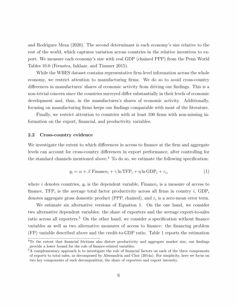
2.2 Cross-country evidence
We investigate the extent to which differences in access to finance at the firm and aggregate
levels can account for cross-country differences in export performance, after controlling for
the standard channels mentioned above.4 To do so, we estimate the following specification:
yi = α + β Financei + γ ln TFPi + η ln GDPi + εi, (1)
where i denotes countries, yi is the dependent variable, Financei is a measure of access to
finance, TFPi is the average total factor productivity across all firms in country i, GDPi
denotes aggregate gross domestic product (PPP, chained), and εi is a zero-mean error term.
We estimate six alternative versions of Equation 1. On the one hand, we consider
two alternative dependent variables: the share of exporters and the average export-to-sales
ratio across all exporters.5 On the other hand, we consider a specification without finance
variables as well as two alternative measures of access to finance: the financing problem
(FP) variable described above and the credit-to-GDP ratio. Table 1 reports the estimation
4To the extent that financial frictions also distort productivity and aggregate market size, our findingsprovide a lower bound for the role of finance-related variables.
5A complementary approach is to investigate the role of financial factors on each of the three componentsof exports to total sales, as decomposed by Alessandria and Choi (2014a). For simplicity, here we focus ontwo key components of such decomposition, the share of exporters and export intensity.
6

Table 1: Cross-country evidence
Share of exporters Exports / Sales
(1) (2) (3) (4) (5) (6)
Financing problem -0.211 -0.407
(0.069) (0.000)
Aggregate Credit / GDP 0.296 0.130
(0.000) (0.040)
TFP (log) 0.501 0.460 0.304 -0.138 -0.216 -0.199
(0.000) (0.000) (0.002) (0.197) (0.033) (0.113)
Aggregate GDP (log) -0.004 -0.008 -0.022 -0.006 -0.015 -0.011
(0.689) (0.391) (0.031) (0.533) (0.101) (0.355)
Constant -0.239 -0.034 0.085 0.687 1.081 0.758
(0.063) (0.841) (0.562) (0.000) (0.000) (0.000)
R-squared 0.196 0.231 0.356 0.026 0.198 0.066
Obs. 93 93 84 93 93 84
Note: Exports/sales and TFP are averages across all firms within each country. Exports/Sales is averaged conditional onexporting. Financing problem is the share of firms in each country that report access to finance to be at least a moderate prob-lem for the firm’s operations. All variables except aggregate Credit/GDP and aggregate GDP correspond to manufacturingfirms. p-values are reported in parentheses.
results. Appendix A presents summary statistics for the variables used throughout.
2.2.1 Extensive margin: Share of exporters
The first three columns of Table 1 report the estimated values using the share of exporters
as the dependent variable. We find that both finance variables are statistically significant
in accounting for variation in the shares of exporters across countries, even after controlling
for firm-level average productivity and aggregate market size. Countries with more firms
reporting access to finance as a problem tend to feature a lower fraction of exporting firms.
Similarly, economies with a lower aggregate credit-to-GDP ratio have fewer exporters.
7
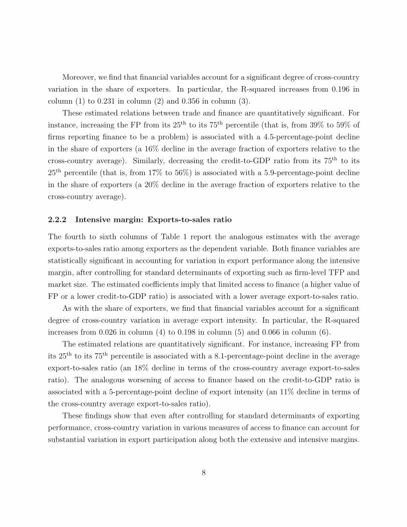
Moreover, we find that financial variables account for a significant degree of cross-country
variation in the share of exporters. In particular, the R-squared increases from 0.196 in
column (1) to 0.231 in column (2) and 0.356 in column (3).
These estimated relations between trade and finance are quantitatively significant. For
instance, increasing the FP from its 25th to its 75th percentile (that is, from 39% to 59% of
firms reporting finance to be a problem) is associated with a 4.5-percentage-point decline
in the share of exporters (a 16% decline in the average fraction of exporters relative to the
cross-country average). Similarly, decreasing the credit-to-GDP ratio from its 75th to its
25th percentile (that is, from 17% to 56%) is associated with a 5.9-percentage-point decline
in the share of exporters (a 20% decline in the average fraction of exporters relative to the
cross-country average).
2.2.2 Intensive margin: Exports-to-sales ratio
The fourth to sixth columns of Table 1 report the analogous estimates with the average
exports-to-sales ratio among exporters as the dependent variable. Both finance variables are
statistically significant in accounting for variation in export performance along the intensive
margin, after controlling for standard determinants of exporting such as firm-level TFP and
market size. The estimated coefficients imply that limited access to finance (a higher value of
FP or a lower credit-to-GDP ratio) is associated with a lower average export-to-sales ratio.
As with the share of exporters, we find that financial variables account for a significant
degree of cross-country variation in average export intensity. In particular, the R-squared
increases from 0.026 in column (4) to 0.198 in column (5) and 0.066 in column (6).
The estimated relations are quantitatively significant. For instance, increasing FP from
its 25th to its 75th percentile is associated with a 8.1-percentage-point decline in the average
export-to-sales ratio (an 18% decline in terms of the cross-country average export-to-sales
ratio). The analogous worsening of access to finance based on the credit-to-GDP ratio is
associated with a 5-percentage-point decline of export intensity (an 11% decline in terms of
the cross-country average export-to-sales ratio).
These findings show that even after controlling for standard determinants of exporting
performance, cross-country variation in various measures of access to finance can account for
substantial variation in export participation along both the extensive and intensive margins.
8

2.3 Firm-level evidence
The analysis above is informative about the potential for differences in access to finance
to account for cross-country differences in exporting performance. However, countries differ
along numerous dimensions, some of which could be correlated with our finance measures. To
address such potential sources of bias, we now conduct an analogous analysis at the firm-level.
This alternative approach allows us to exploit within-country variation in access to finance to
evaluate its potential to account for cross-firm variation in exporting performance. As above,
we do so while simultaneously controlling for standard determinants of export decisions such
as firm-level productivity.6
We estimate the following specification:
yf,i,j,t = αi,j,t + β FPf,i,j,t + γ ln TFPf,i,j,t + εf,i,j,t, (2)
where f , i, j, and t index firms, countries, industries, and time periods, respectively. We focus
on variation within country-industry-year triples by controlling for fixed effects αi,j,t at this
level. We control for our firm-level measure of access to finance FPf,i,j,t (Finance problem,
as described above), and our standard determinant of export performance, TFPf,i,j,t.
Equation 2 is estimated for two alternative dependent variables. On the one hand, we
consider a specification with an indicator variable that is equal to 1 if the firm exports
and zero otherwise. On the other hand, we estimate the specification using the firm-level
export-to-sales ratio conditional on exporting. Table 2 reports the estimation results.
The first column of Table 2 reports the estimated coefficients for the specification with
the exporter indicator variable as the dependent variable. We find that the FP is statistically
significant. Controlling for country, industry, and year fixed effects as well as for firm-level
TFP, firms that report financing to be a problem are 2.7% less likely to be exporters (reducing
the unconditional cross-country probability of exporting by 9.3%).7
The second column reports the analogous estimates for the specification with the exports-
to-sales ratio as the dependent variable. The FP is statistically and economically significant,
with a 1.7-percentage-point lower exports-to-sales ratio than firms that do not report finance
6To the extent that financial frictions also distort firm-level productivity, our findings provide a lower boundfor the role of finance-related variables.
7We interpret the average share of exporters across countries (Table 4 in the appendix) as the unconditionalexport probability.
9

Table 2: Firm-level evidence
Exporter Exports / Sales
Financing problem -0.027 -0.017
(0.000) (0.011)
TFP (log) 0.038 0.010
(0.000) (0.119)
Constant 0.312 0.451
(0.000) (0.000)
R-squared 0.268 0.430
Obs. 43,608 14,527
Note: Exporter is equal to 1 if firms export and 0 otherwise. Exports/Salesis conditional on exporting. Financing problem is equal to 1 if firms reportaccess to finance to be at least a moderate problem for its operations. Theregressions control for country-industry-year fixed effects. All variablescorrespond to manufacturing firms. p-values are reported in parentheses.
to be a problem for their operations (reducing the exports-to-sales ratio by 3.7% relative to
the unconditional cross-country average; see Table 4 in the appendix).
Thus, we find that finance is significantly associated with variation in firm-level export
performance along both the extensive and intensive margins, even after controlling for stan-
dard exporting determinants such as productivity. We also find evidence consistent with
standard firm-level theories of international trade that associate higher productivity with
higher export performance.
2.4 Discussion and related literature
While the empirical evidence discussed in this section suggests that financial factors may
have important implications for international trade, a key identification problem remains.
At the firm-level, it is difficult to determine whether low use of external finance is due to a
limited need for credit (perhaps because firms face low demand for their goods), or due to a
limited credit supply. Similarly, at the aggregate level, low credit-to-GDP ratios may arise
from either low aggregate credit demand due to limited growth opportunities or because of
10
severe financial frictions. For instance, one alternative interpretation of our findings is that
they might reflect reverse causality, with non-exporting firms having less access to finance.
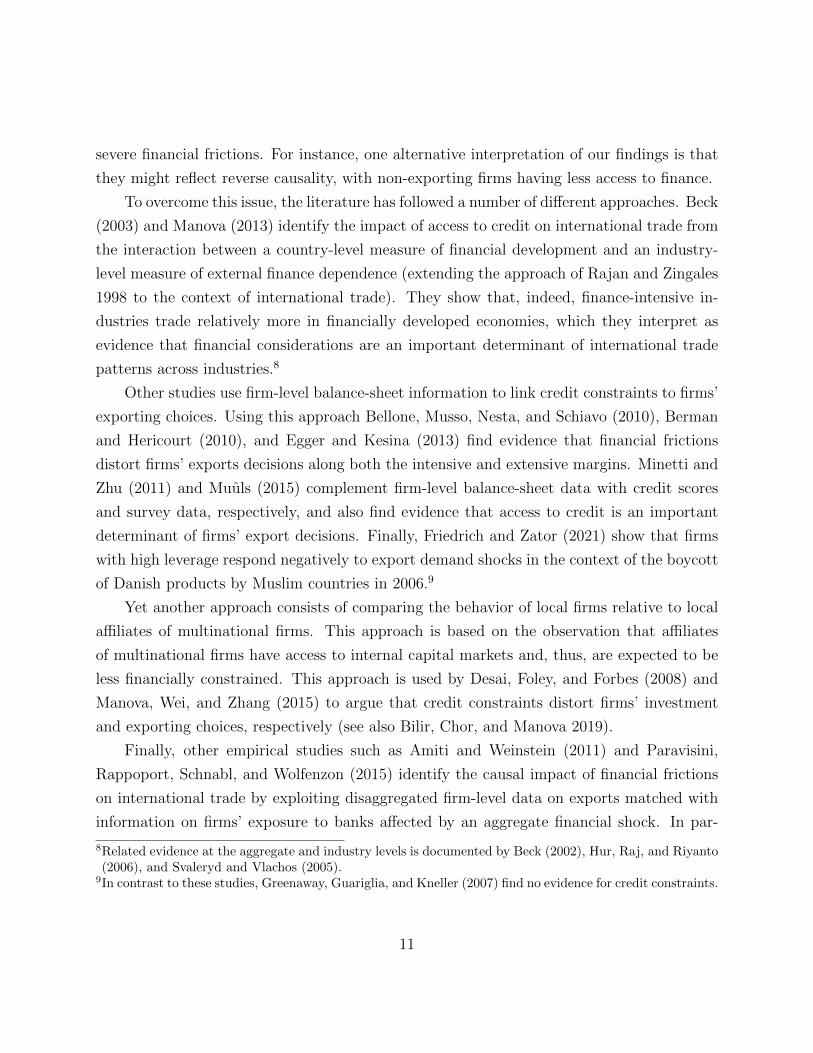
To overcome this issue, the literature has followed a number of different approaches. Beck
(2003) and Manova (2013) identify the impact of access to credit on international trade from
the interaction between a country-level measure of financial development and an industry-
level measure of external finance dependence (extending the approach of Rajan and Zingales
1998 to the context of international trade). They show that, indeed, finance-intensive in-
dustries trade relatively more in financially developed economies, which they interpret as
evidence that financial considerations are an important determinant of international trade
patterns across industries.8
Other studies use firm-level balance-sheet information to link credit constraints to firms’
exporting choices. Using this approach Bellone, Musso, Nesta, and Schiavo (2010), Berman
and Hericourt (2010), and Egger and Kesina (2013) find evidence that financial frictions
distort firms’ exports decisions along both the intensive and extensive margins. Minetti and
Zhu (2011) and Muuls (2015) complement firm-level balance-sheet data with credit scores
and survey data, respectively, and also find evidence that access to credit is an important
determinant of firms’ export decisions. Finally, Friedrich and Zator (2021) show that firms
with high leverage respond negatively to export demand shocks in the context of the boycott
of Danish products by Muslim countries in 2006.9
Yet another approach consists of comparing the behavior of local firms relative to local
affiliates of multinational firms. This approach is based on the observation that affiliates
of multinational firms have access to internal capital markets and, thus, are expected to be
less financially constrained. This approach is used by Desai, Foley, and Forbes (2008) and
Manova, Wei, and Zhang (2015) to argue that credit constraints distort firms’ investment
and exporting choices, respectively (see also Bilir, Chor, and Manova 2019).
Finally, other empirical studies such as Amiti and Weinstein (2011) and Paravisini,
Rappoport, Schnabl, and Wolfenzon (2015) identify the causal impact of financial frictions
on international trade by exploiting disaggregated firm-level data on exports matched with
information on firms’ exposure to banks affected by an aggregate financial shock. In par-
8Related evidence at the aggregate and industry levels is documented by Beck (2002), Hur, Raj, and Riyanto(2006), and Svaleryd and Vlachos (2005).
9In contrast to these studies, Greenaway, Guariglia, and Kneller (2007) find no evidence for credit constraints.
11

ticular, controlling for detailed information on the types of goods and destinations to which
firms export, these studies identify the role of credit on exports from systematic variation in
export performance across firms that obtain credit from banks with heterogeneous exposure
to an aggregate financial shock.
Overall, this large and diverse empirical literature suggests there is a significant link
between trade and finance. In the following sections, we introduce an alternative way to
address the identification problem: The use of a quantitative model of heterogeneous firms
estimated to match salient features of firm-level data to investigate the link between access
to finance and export decisions. We also discuss the related theoretical and quantitative
literature.
3 Financial frictions and trade: An analytical framework
A complementary strategy to assessing the importance of financial frictions on international
trade is to quantitatively analyze the implications of a structural model of trade with credit
market frictions. After formulating the model, one can calibrate it to match salient features
of the data and use it to quantify the impact of financial frictions on key outcomes of interest.
In particular, to the extent that the model indeed captures key features of financial frictions,
one can use it to conduct counter-factual analysis, such as evaluating their role in accounting
for the response to large devaluations or trade liberalization.
One advantage of this approach is that it allows for an internally consistent analysis
of the impact of financial frictions on export decisions while being explicit about the as-
sumptions underlying the mechanism under analysis. However, it also has its limitations:
a drawback of this approach is that it narrows the analysis to the mechanisms featured by
the model, abstracting from other potentially relevant channels through which finance might
interact with international trade. Thus, we view the quantitative work presented here as
complementary to empirical studies: empirics guide modeling choices, while quantitative and
theoretical results inform further empirical analyses.
In the rest of this section, we present a quantitative model to interpret the evidence from
Section 2 and to quantify the impact of financial frictions. The model described below is a
simplified version of the setup developed in Kohn, Leibovici, and Szkup (2016), Kohn, Lei-
bovici, and Szkup (2020a), Kohn, Leibovici, and Szkup (2020b), and Leibovici (2021). We
12

use this framework to study the channels through which financial frictions affect firms’ de-
cisions and their aggregate consequences. We conclude this section by discussing alternative
ways to model financial frictions and mechanisms from which we abstract here.
3.1 Model
We consider a small open economy populated by a unit measure of entrepreneurs who pro-
duce differentiated varieties that are sold domestically and abroad.10 The economy is also
populated by final goods producers who produce final goods by aggregating domestic vari-
eties purchased from entrepreneurs and imported varieties purchased from the rest of the
world.
Entrepreneurs Entrepreneurs are risk-averse, with preferences over consumption of final
goods given by
∞∑t=0
βtc1−γit
1− γ, (3)
where i ∈ [0, 1] indexes entrepreneurs. Each entrepreneur produces differentiated varieties
by operating a production technology
yit = zitkαitn
1−αit , (4)
where zit denotes an idiosyncratic level of productivity, kit is the capital stock, nit is the
amount of labor hired, and α ∈ (0, 1) is the capital share. Capital is accumulated internally
and depreciates at the rate δ ∈ (0, 1). Idiosyncratic productivity follows an AR(1) process:
ln zit = (1− ρ)µz + ρzi,t−1 + εit, (5)
where εit ∼ N(0, σε) and µz is the average level of productivity. Finally, entrepreneurs are
endowed with one unit of labor that they supply inelastically to a competitive labor market.
Entrepreneurs are monopolistically competitive and sell their varieties to domestic final
goods producers and to the rest of the world. As in Melitz (2003), exporting requires
10We interchangeably refer to entrepreneurs as firms.
13

entrepreneurs to pay a fixed export cost F > 0 denominated in units of labor, and a variable
cost τ that requires them to ship τ > 1 per unit that arrives at the destination.
Entrepreneurs have access to financial markets, where they can borrow or save by trading
a one-period non-contingent bond. However, borrowing is constrained to be at most a
fraction θ of their capital stock at the time of repayment. The amount borrowed (i.e., debt),
dit, has to satisfy
dit ≤ θki,t+1 (6)
and the natural borrowing limit. Financial markets are integrated internationally, and there
is a perfectly elastic supply of bonds from the rest of the world at a given interest rate r > 0.
The timing of the model is similar to the one considered in Buera and Moll (2015) and
others. Entrepreneurs begin the period by hiring labor, producing their variety, and then
selling that variety in each of the markets in which they choose to operate. They pay for
labor and export costs (if applicable) and repay their debt from the previous period. Then,
they choose their consumption and the amount of net worth to begin with next period. At
the end of the period, after the above decisions have been made, entrepreneurs observe the
following period’s productivity shock and choose the composition of next period’s net worth
between debt and physical capital.11
Final goods producers Final goods producers purchase varieties from entrepreneurs and
the rest of the world and aggregate them to produce final goods with a constant elasticity
of substitution technology. They are perfectly competitive, so they take all prices as given.
The problem is given by
maxYh,t −∫ 1
0
ph,ityh,itdi− ξtpmym,t
s.t. Yt =
[∫ 1
0
yσ−1σ
hi,t di+ yσ−1σ
m,t
] σσ−1
,
where Yh,t is the amount of final goods produced; {ph,it}i∈[0,1] and pm are the prices of varieties
sold by entrepreneurs and the rest of the world, respectively; {yh,it}i∈[0,1] and ym,t denote
11As in Buera and Moll (2015), these timing assumptions imply that the relevant endogenous state variableis net worth ait = kit − dit
1+r , which reduces the number of state variables.
14

the amount of domestic and imported varieties purchased, respectively; and σ denotes the
elasticity of substitution between domestic and imported varieties. We normalize prices
relative to the price of the domestic final goods and ξ is the relative price of the foreign
final goods in units of the domestic final goods (the real exchange rate). The solution to
this problem is given by yh,it = (ph,it)−σ Yh,t and ym,t = (pm)−σYh,t, which are the demand
schedules faced by entrepreneurs and the rest of the world, respectively.
Rest of the world The rest of the world demands varieties from entrepreneurs (the
economy’s exports) and supplies varieties to final goods producers (the economy’s imports).
The rest of the world’s demand for varieties produced by entrepreneurs is downward sloping
with the same constant elasticity of substitution σ as the domestic demand for varieties:
yf,t = (pf,t)−σYf , where Yf is the exogenous amount of final goods produced in the rest of
the world and pf,t is the price charged in units of the foreign final goods.
Entrepreneurs’ problem Given our timing assumptions, the entrepreneurs’ problem
can be divided into a consumption-savings problem and a net worth composition problem.12
Let v (k, d, z) denote the value function of an entrepreneur with capital k, debt d, and
productivity z, who makes consumption-savings as well as production decisions. Let g (a′, z′)
denote the value function of an entrepreneur at the end of a period with next period’s net
worth a′ and productivity z′, who decides how to allocate her net worth between capital k
and debt d1+r
. Then,
v (k, d, z) = maxc,a′≥0
c1−γ
1− γ+ Ez′ [g (a′, z′)]
subject to c+ a′ + d = w + (1− δ)k + π(k, z),
12To ease the exposition, we restrict attention to a stationary environment in which all aggregate variablesare constant; we omit entrepreneur-specific indexes i to simplify the notation.
15

where π(k, z) denotes profits earned this period given capital k and productivity z. En-
trepreneurs make production choices to maximize profits. These are given by
π(k, z) = maxph,yh,pf ,yf ,n,e∈{0,1}
phyh + e ξpfyf − wn− ewF
subject to yh + τyf = zkαn1−α, yh = p−σh Yh, yf = p−σf Yf ,
where e denotes the entrepreneur’s export choice (e = 1 if she exports, e = 0 otherwise).
The entrepreneur’s net worth allocation between debt and capital is given by
g(a′, z′) = maxk′,d′
βv(k′, d′, z′)
subject to
d′ = (1 + r)(k′ − a′) (7)
k′ ≤ 1 + r
1 + r − θa′. (8)
Note that Equation 8 results from combining Equations 6 and 7. Thus, even though the
borrowing constraint in Equation 6 limits the amount of debt for entrepreneurs, it implies a
constraint on the total amount of capital they can accumulate.
Stationary equilibrium Let S ≡ A×Z denote the state space of entrepreneurs, and let
s ∈ S denote an element of the state space. For a given interest rate r, a recursive stationary
competitive equilibrium of this economy consists of a wage and real exchange rate {w, ξ},policy functions {d′(s), k′(s), e(s), c(s), n(s), yh(s), yf (s), ph(s), pf (s), Yh, ym}, value functions
v and g, and a stationary measure φ : S → [0, 1] such that (i) policy and value functions
solve the problems of entrepreneurs and final goods producers and (ii) labor and final goods
markets clear.
Numerical solution We solve the model numerically using global methods, approximat-
ing the value functions at a discrete number of grid points of the state variables z and a. We
discretize the stochastic process followed by productivity z using Tauchen’s method (Tauchen
1986). We approximate the value function through value function iteration, obtaining the
optimal net worth accumulation policy in each state.
16

3.2 The effects of financial frictions on international trade
In this section, we study the mechanisms through which financial frictions distort export
decisions. We begin our analysis by discussing how borrowing constraints distort capital
choices, since this is a channel through which financial frictions end up distorting trade flows.
We then analyze how financial frictions distort export volumes conditional on exporting
(intensive margin) and discuss their impact on entrepreneurs’ decision to export (extensive
margin).
To highlight the role of financial frictions, we consider three versions of the model: (i) a
general equilibrium model with no financial frictions (θ ≥ 1 + r);13 (ii) a partial equilibrium
model with financial frictions, θ ∈ (0, 1 + r), with prices fixed at the level of the frictionless
economy; and (iii) a general equilibrium model with financial frictions, θ ∈ (0, 1 + r). Con-
trasting the implications of the first two models allows us to characterize the direct impact
of financial frictions on economic outcomes. Examining the general equilibrium model with
financial frictions allows us to assess the interplay between financial frictions and general
equilibrium forces. The parametrization of these models is described in the appendix.
3.2.1 Capital choice
Figure 1 plots the relation between capital choice and net worth across the three models for
a firm with relatively low productivity (left panel) and relatively high productivity (right
panel). We note first that in the frictionless model, entrepreneurs’ choices of capital do not
depend on entrepreneurs’ net worth (red dashed line). Thus, regardless of net worth, in this
model, entrepreneurs can always operate with the first-best amount of physical capital.
Consider now the economy with financial frictions, but with prices fixed at the values of
the frictionless equilibrium. We see that entrepreneurs’ capital choice is now increasing in
net worth and that for sufficiently low levels of net worth, their capital choice is below the
frictionless level. In addition, note that relatively unproductive firms require low levels of
net worth to be able to operate at the optimal level of capital. In contrast, firms with high
productivity need to accumulate a high amount of net worth before reaching the optimal
level of capital stock.14 It follows that it takes a while before firms that receive a good
13If θ ≥ 1 + r, then the financial constraint is never binding.14The fact that relatively unproductive firms require less net worth to achieve their optimal scale implies
that in the economy with financial frictions domestic producers’ choices are less distorted than those of
17

productivity shock are able to achieve their optimal scale. This implies that, on average,
new exporters will begin exporting while being severely financially constrained (in the sense
that their capital will be far from its optimal unconstrained level), and it will take them
a while to accumulate enough assets to achieve their optimal scale. Kohn, Leibovici, and
Szkup (2016) use this observation to argue that financial frictions are an important driver
of new exporter dynamics.
Figure 1: Capital choice
Net Worth
Capital
Financial Frictions (GE)
Frictionless
Financial Frictions (PE)
(a) Low Productivity
Net Worth
Capital
Financial Frictions (GE)
Frictionless
Financial Frictions (PE)
(b) High Productivity
Note: Optimal choice of capital as a function of net worth for an entrepreneur with relatively lowproductivity (left panel) and high productivity (right panel). See the appendix for calibration details. Inthe partial equilibrium version of the model with financial frictions, prices are set at their frictionless levels.GE refers to general equilibrium and PE refers to partial equilibrium.
The above observations also apply to the model with financial frictions in general equi-
librium. However, the inability of some entrepreneurs to operate at the optimal level of
capital decreases demand for labor and the demand for final goods, decreasing the real wage
and increasing the real exchange rate. Since labor input is cheaper than in the frictionless
economy, unconstrained entrepreneurs choose higher capital than they would in the absence
of borrowing constraints. Then, as can be observed in Figure 1, entrepreneurs with low net
worth have to operate with capital below their frictionless level while entrepreneurs with
new exporters.
18
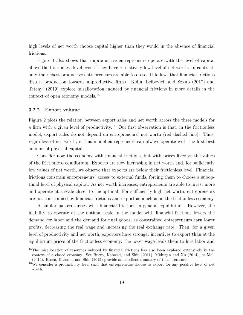
high levels of net worth choose capital higher than they would in the absence of financial
frictions.
Figure 1 also shows that unproductive entrepreneurs operate with the level of capital
above the frictionless level even if they have a relatively low level of net worth. In contrast,
only the richest productive entrepreneurs are able to do so. It follows that financial frictions
distort production towards unproductive firms. Kohn, Leibovici, and Szkup (2017) and
Tetenyi (2019) explore misallocation induced by financial frictions in more details in the
context of open economy models.15
3.2.2 Export volume
Figure 2 plots the relation between export sales and net worth across the three models for
a firm with a given level of productivity.16 Our first observation is that, in the frictionless
model, export sales do not depend on entrepreneurs’ net worth (red dashed line). Thus,
regardless of net worth, in this model entrepreneurs can always operate with the first-best
amount of physical capital.
Consider now the economy with financial frictions, but with prices fixed at the values
of the frictionless equilibrium. Exports are now increasing in net worth and, for sufficiently
low values of net worth, we observe that exports are below their frictionless level. Financial
frictions constrain entrepreneurs’ access to external funds, forcing them to choose a subop-
timal level of physical capital. As net worth increases, entrepreneurs are able to invest more
and operate at a scale closer to the optimal. For sufficiently high net worth, entrepreneurs
are not constrained by financial frictions and export as much as in the frictionless economy.
A similar pattern arises with financial frictions in general equilibrium. However, the
inability to operate at the optimal scale in the model with financial frictions lowers the
demand for labor and the demand for final goods, as constrained entrepreneurs earn lower
profits, decreasing the real wage and increasing the real exchange rate. Then, for a given
level of productivity and net worth, exporters have stronger incentives to export than at the
equilibrium prices of the frictionless economy: the lower wage leads them to hire labor and
15The misallocation of resources induced by financial frictions has also been explored extensively in thecontext of a closed economy. See Buera, Kaboski, and Shin (2011), Midrigan and Xu (2014), or Moll(2014). Buera, Kaboski, and Shin (2015) provide an excellent summary of that literature.
16We consider a productivity level such that entrepreneurs choose to export for any positive level of networth.
19

Figure 2: Export volume
Net Worth
Export
Sal
es
Financial Frictions (GE)
Frictionless
Financial Frictions (PE)
Note: Optimal export volume as a function of net worth, given a sufficiently high level of productivity suchthat firms export. See the appendix for calibration details. In the partial equilibrium version of the modelwith financial frictions, prices are set at their frictionless levels. GE refers to general equilibrium and PErefers to partial equilibrium.
increase their scale, while the higher real exchange rate increases the foreign demand for
domestic varieties, raising the returns to exporting. Then, as observed in Figure 2, exports
are below the frictionless level for entrepreneurs with low net worth but they are above the
frictionless level for sufficiently high levels of net worth.
Finally, it is worth pointing out that in this simple framework, export intensity (defined
as the ratio of export sales to total exports) is undistorted by the presence of financial
frictions. That is, in all versions of the model, all exporters have the same export intensity.
Kohn, Leibovici, and Szkup (2016) consider a version of this model with working capital
needs that are asymmetric across the domestic and foreign markets and show that in such
model, export intensity is an increasing function of assets.
3.2.3 Decision to export
We next examine the effect of financial frictions on firms’ decision to export. To do so,
Figure 3 characterizes the export threshold as a function of net worth and productivity for
20
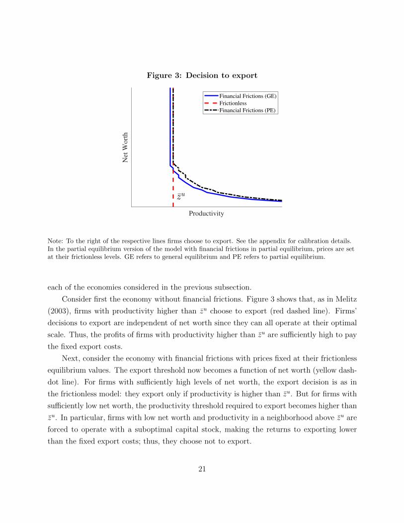
Figure 3: Decision to export
Net
Wort
h
Productivity
Financial Frictions (GE)
Frictionless
Financial Frictions (PE)
Note: To the right of the respective lines firms choose to export. See the appendix for calibration details.In the partial equilibrium version of the model with financial frictions in partial equilibrium, prices are setat their frictionless levels. GE refers to general equilibrium and PE refers to partial equilibrium.
each of the economies considered in the previous subsection.
Consider first the economy without financial frictions. Figure 3 shows that, as in Melitz
(2003), firms with productivity higher than zu choose to export (red dashed line). Firms’
decisions to export are independent of net worth since they can all operate at their optimal
scale. Thus, the profits of firms with productivity higher than zu are sufficiently high to pay
the fixed export costs.
Next, consider the economy with financial frictions with prices fixed at their frictionless
equilibrium values. The export threshold now becomes a function of net worth (yellow dash-
dot line). For firms with sufficiently high levels of net worth, the export decision is as in
the frictionless model: they export only if productivity is higher than zu. But for firms with
sufficiently low net worth, the productivity threshold required to export becomes higher than
zu. In particular, firms with low net worth and productivity in a neighborhood above zu are
forced to operate with a suboptimal capital stock, making the returns to exporting lower
than the fixed export costs; thus, they choose not to export.
21

Finally, consider the model with financial frictions in general equilibrium. As discussed
in Section 3.2.2, this economy features a lower wage and a higher real exchange rate than
the frictionless setup since there is a lower demand for labor and for the domestic final
goods. Thus, production costs are lower and foreign demand for domestic varieties is higher,
which make exporting more attractive. Thus, the export threshold shifts to the left of
its counterpart for the economy with financial frictions but frictionless equilibrium prices.
This implies that some low-productivity but high-net-worth firms that would choose not
to export in the frictionless economy now choose to do so. These unproductive but high-
net-worth entrepreneurs replace those with high productivity but low net worth who are
prevented from exporting due to financial frictions.
The above discussion shows that the direct impact of financial frictions is to prevent
productive firms with low net worth from exporting, leading to a lower share of exporters.
But the indirect impact via general equilibrium effects is to allow unproductive entrepreneurs
with high net worth to export, increasing the share of firms that export. Thus, the overall
effect of financial frictions on the share of exporters is ambiguous.
3.3 Discussion of model assumptions
The setup presented in Section 3.1 captures the key channels through which financial frictions
distort international trade. Nevertheless, it is a stylized model that makes some simplifying
assumptions and abstracts from several mechanisms that might strengthen or attenuate the
effects of financial frictions. In this section, we discuss some of these additional mechanisms
and the implications of our simplifying assumptions.
Modeling of financial frictions Following Buera, Kaboski, and Shin (2011) and Midri-
gan and Xu (2014), we model financial frictions by assuming that entrepreneurs accumulate
capital internally and face a collateral constraint on the amount of debt they can issue.
Buera and Moll (2015) show that this setup is equivalent to assuming that entrepreneurs
rent capital from capital markets and face a constraint that limits the amount of capital
they can rent to a fraction of their wealth (see also Moll 2014 and Buera and Shin 2013).
A distinguishing feature of the financing constraint that we study is that the maxi-
mum amount that firms can borrow is only determined by the capital stock installed at the
time of repayment; in particular, it is not directly affected by firms’ productivity or net
22

worth. Closer to Buera, Kaboski, and Shin (2011), Buera and Shin (2017), and Gopinath,
Kalemli-Ozcan, Karabarbounis, and Villegas-Sanchez (2017), one could consider a borrowing
constraint dt+1 ≤ θ(at, zt)kt+1, where θ(a, z) is increasing in net worth and productivity. In
our context, the net impact on productive but low net worth firms, whose export decisions
are primarily distorted, would be ambiguous.
Brooks and Dovis (2020) consider a financial constraint in which the maximum amount
that can be borrowed depends on future firm profitability, following Albuquerque and Hopen-
hayn (2004). They show that such forward-looking constraints imply that the gains from
trade liberalization are identical to those in a model without financial frictions. Further
work is needed to better understand the type of constraints firms face and whether they are
primarily backward or forward looking.17
The papers above assume that the relative value of collateral and debt is fixed. Kiyotaki
and Moore (1997) instead consider a constraint dt+1 ≤ θPk,tkt+1, where Pk is the price of
capital in units of consumption. In their model, the price of capital is endogenous, leading
to the value of collateral varying with aggregate conditions, amplifying the macroeconomic
impact of aggregate shocks (see also Bernanke, Gertler, and Gilchrist 1999). Kohn, Lei-
bovici, and Szkup (2020b) study constraints of this type to analyze the impact of changes
in intermediate input and capital goods tariffs.
Finally, most of the literature that studies the effects of financial frictions on international
trade abstract from long-term borrowing. Notable exceptions are Gross and Verani (2013)
and Bergin, Feng, and Lin (2021). The former studies how financial frictions affect firms’
export decisions and growth in an environment with long-term contracts as in Clementi and
Hopenhayn (2006). The latter introduces an endogenous choice between long-term debt and
equity financing into a trade model with heterogeneous firms and export entry.
Working capital needs and financing of fixed costs Our model abstracts from
working capital needs. Requiring firms to pay for a fraction of the labor costs in advance
might tighten financing constraints, amplifying the distortions. Similarly, we do not require
17For instance, Aguirre, Tapia, and Villacorta (2021) provide evidence in support of the importance ofbackward-looking financial constraints. In particular, they use Chilean firm-level data to document that(i) the reaction of investment to productivity shocks depends on the level of collateral, with larger responsesfrom unconstrained firms; and that (ii) productive firms accumulate wealth after positive and persistentproductivity shocks, with larger effects across firms with lower wealth levels.
23

firms to pay fixed costs of exporting in advance (as in Chaney 2016 or Leibovici 2021).18
Such additional financial needs are likely to force low net worth firms to operate at an even
lower scale than in our model, further discouraging them from exporting.
Sunk export entry costs Our model abstracts from sunk export entry costs, that is,
one-time costs paid by firms only when they start exporting. Sunk export entry costs make
firms’ export decisions dynamic and were first introduced to account for hysteresis in export-
ing decisions (Baldwin and Krugman 1989, Dixit 1989), generating equilibria with relatively
unproductive exporters and productive non-exporters. Alessandria and Choi (2014a,b) ad-
ditionally show that sunk export entry costs are important to account for key features of
export dynamics, while Alessandria, Pratap, and Yue (2014) argue that they are important
to account for the slow growth of exports following large devaluations.
We abstract from sunk export entry costs motivated by Kohn, Leibovici, and Szkup
(2016), who show that financial frictions can generate the observed coexistence of relatively
unproductive exporters with productive non-exporters, as sunk costs do.19 Manova (2013)
and Leibovici (2021) study economies with both financial frictions and sunk export entry
costs where the latter exacerbate the distortionary impact of financial frictions.
Multiple export destinations Our model considers exporting as a discrete decision
among two options: being an exporter or a non-exporter. This approach abstracts from the
more granular choice made by firms across the set of destinations to export to if they choose
to do so. As argued by Manova (2013), financial frictions can also distort the set of desti-
nations to which firms export. She considers a model where exporting to each destination
is associated with a destination-specific fixed export cost and the financing of fixed export
costs is subject to financial frictions. This approach implies that firms with limited access
to internal and external funds export to fewer destinations. Consistent with this implication
of the model, Manova (2013) documents that finance-intensive industries export to fewer
destinations in countries with less financial development.
18Chaney (2016) considers a model with financing constraints that only distort the payment of fixed exportcosts. Thus, in this environment financial frictions have “direct” effects only on the extensive margin. Hestudies the coexistence of competitive devaluations and revaluations.
19Abstracting from sunk export entry costs also simplifies the numerical solution of the model, since exportstatus becomes a state variable in economies with sunk export entry costs.
24

International financial integration In our model, the economy is fully integrated
with international financial markets, allowing agents to save or borrow at an exogenous world
interest rate r. Under either international financial autarky or imperfect financial integration,
the interest rate would respond endogenously to the degree of financial development. As
borrowing increases with financial development, the interest rate also increases to restore
balance between demand and supply in financial markets. The increase of the interest rate
has two opposite effects, with an ambiguous overall impact. On the one hand, it increases
the cost of debt and effectively tightens the borrowing constraint, amplifying distortions. On
the other hand, it encourages savings, leading to higher average net worth.
Tetenyi (2019) investigates the impact of financial integration on the gains from trade
in a similar model with financial frictions. Under international financial integration, trade
liberalization exacerbates the misallocation due to financial frictions. However, trade liber-
alization has minor effects on misallocation under international financial autarky.
Occupational choice Our model also abstracts from individuals’ occupational choice
between being workers or entrepreneurs, among other occupational choices they might face.
Kohn, Leibovici, and Szkup (2017) and Leibovici (2021) study economies in which individuals
choose whether to be workers or entrepreneurs. Without financial frictions, the occupational
choice is characterized by a productivity threshold zu such that individuals with z ≥ zu
choose to be entrepreneurs, and the rest choose to be workers. Financial frictions distort
this decision by making productive individuals with low net worth to be workers rather than
entrepreneurs. It follows that financial frictions distort firms’ entry, further distorting the
set of firms that choose to export in equilibrium. Moreover, occupational choice leads to
misallocation of talent across occupations, amplifying the misallocation of capital and labor
relative to an economy without occupational choice.20
20There exists a large literature that investigates the impact of financial frictions on occupational choices (seeBuera, Kaboski, and Shin 2015 for a detailed summary). Similarly, yet in a framework with homogeneousfirms, Bergin, Feng, and Lin (2018a,b) stress the importance of financial frictions in determining firms’entry decisions and show that this mechanism can moderate the impact of financial shocks on aggregateoutput but can lead to a prolonged export decline.
25
4 Aggregate and firm-level implications of financial frictions
We now discuss how alternative versions of the framework presented above have been used
to quantitatively study various implications of financial frictions on international trade. We
focus on their implications for firm-level dynamics and for aggregate and industry-level out-
comes, and conclude with their implications for the aggregate dynamics following aggregate
shocks such as large devaluations or trade liberalization. For each of these dimensions, we
provide an in-depth description of a particular paper while also discussing various related
studies.
4.1 Implications for firm-level dynamics
We begin by focusing on the implications of financial frictions for the dynamics of new
exporters. In the data, firm-level exports and export intensity are increasing on average
in the length of export spells, while the probability that firms stop exporting decreases
as firms continue to export. Ruhl and Willis (2017) first documented these dynamics using
Colombian plant-level data and showed that standard models of international trade generate
new exporter dynamics at odds with the data.21 These findings suggest that the dynamics
of new exporters might be informative about the underlying frictions affecting firms’ export
decisions.
Kohn, Leibovici, and Szkup (2016) show that introducing financial frictions to a standard
model of international trade can reconcile its implications for new exporter dynamics while
continuing to account for key empirically-consistent implications of these models along other
dimensions.22 To do so, they consider a simplified version of the framework presented in the
previous section. Firms are assumed to use labor as their only input subject to both working
capital and collateral constraints. That is, firms have to pay a fraction of their wage bill in
advance and have to post collateral to access external funds. Furthermore, working capital
requirements are assumed to be asymmetric across markets, with exports requiring a higher
fraction of the wage bill to be paid upfront.23 The combined working capital and collateral
21Similar patterns of new exporter dynamics have also been documented for Chile (Kohn, Leibovici, andSzkup 2016) and Ireland (Fitzgerald, Haller, and Yedid-Levi 2016).
22Gross and Verani (2013) reach similar conclusions using a multi-country model with endogenous financialconstraints that arise due to asymmetric information as in Clementi and Hopenhayn (2006).
23See Kohn, Leibovici, and Szkup (2016) for evidence on asymmetric working capital needs across markets.
26

constraint is given by
αwtnit + eit [wtF + wtn∗it] ≤ λait, (9)
where eit is an indicator function equal to 1 if firm i exports in period t and zero otherwise;
F denotes the fixed costs denominated in labor units; wt is the wage rate; ait denotes net
worth; and nit and n∗it denote the labor hired to produce for the domestic and foreign markets,
respectively. Finally, α denotes the share of labor costs used for domestic sales that needs
to be paid in advance. All export-related costs, including fixed export costs, are assumed to
be paid fully in advance. Firms can either pay these costs out of their net worth ait or by
borrowing up to a multiple λ− 1 ≥ 1 of their net worth.24
The gradual growth of new exporters’ net worth is the key channel that allows the model
to capture the stylized facts described above, as shown in Panels (a)-(c) of Figure 4. Firms
typically start exporting after receiving a positive productivity shock but with a limited net
worth, so they are initially constrained and unable to produce at the optimal scale. As
new exporters increase their net worth, they relax their borrowing constraints and increase
their scale. This allows them to gradually increase their exports, making exporting more
attractive and, thus, decreasing the probability that they stop exporting. Thus, financial
frictions act as sunk costs in inducing hysteresis: a firm that exports in a given period
has a higher probability of exporting the following period. Finally, the model implies that
new exporters initially export a small fraction of their total sales and that this share grows
gradually as firms continue to export: since exports require relatively more working capital,
the opportunity cost of using funds for exports in terms of forgone domestic sales decreases as
exporting firms accumulate net worth and relax their borrowing constraints, so firms choose
to export a higher fraction of their total production.25
Kohn, Leibovici, and Szkup (2016) show that their model can also account for additional
24Net worth constrains total production similarly to Equation 8, with λ ≡ 1+r1+r−θ .
25Complementary explanations for these dynamics include search frictions (Eaton, Eslava, Jinkins, Krizan,and Tybout 2014), slow market penetration (Arkolakis 2010), capital adjustment costs (Rho and Rodrigue2016), or learning about uncertain demand (Nguyen 2012 and Albornoz, Pardo, Corcos, and Ornelas2012). Alessandria, Choi, and Ruhl (2021) generate these export dynamics by allowing exporters to investin lowering their future variable trade costs, and the authors use their framework to evaluate the welfaregains from trade liberalization. Alessandria and Avila (2020) use the same framework to evaluate thewelfare gains from trade reforms that Colombia underwent in the 1980s and early 1990s. Alessandria,Arkolakis, and Ruhl (2021) provide an extensive review of the literature that studies the dynamics of firmsin foreign markets and their aggregate implications.
27
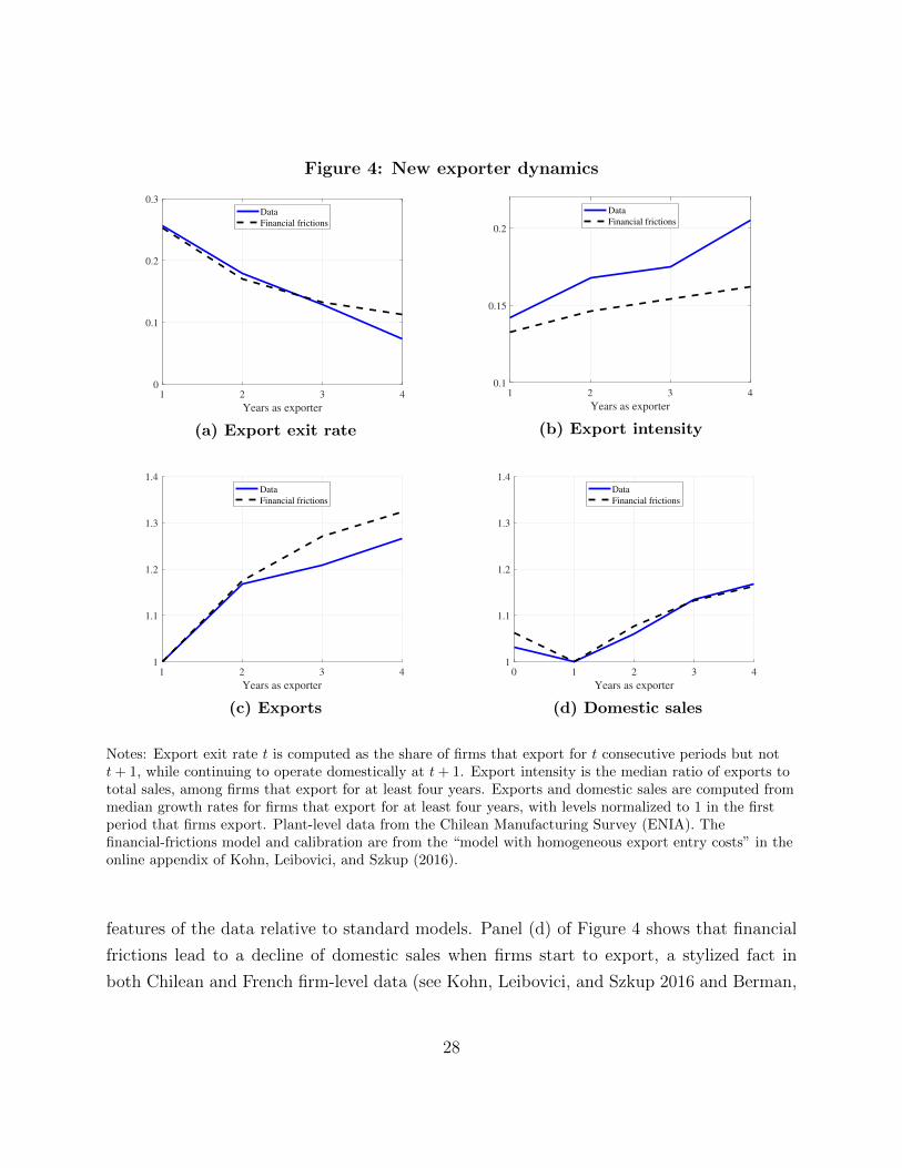
Figure 4: New exporter dynamics
1 2 3 4
Years as exporter
0
0.1
0.2
0.3
Data
Financial frictions
(a) Export exit rate
1 2 3 4
Years as exporter
0.1
0.15
0.2
Data
Financial frictions
(b) Export intensity
1 2 3 4
Years as exporter
1
1.1
1.2
1.3
1.4
Data
Financial frictions
(c) Exports
0 1 2 3 4
Years as exporter
1
1.1
1.2
1.3
1.4
Data
Financial frictions
(d) Domestic sales
Notes: Export exit rate t is computed as the share of firms that export for t consecutive periods but nott+ 1, while continuing to operate domestically at t+ 1. Export intensity is the median ratio of exports tototal sales, among firms that export for at least four years. Exports and domestic sales are computed frommedian growth rates for firms that export for at least four years, with levels normalized to 1 in the firstperiod that firms export. Plant-level data from the Chilean Manufacturing Survey (ENIA). Thefinancial-frictions model and calibration are from the “model with homogeneous export entry costs” in theonline appendix of Kohn, Leibovici, and Szkup (2016).
features of the data relative to standard models. Panel (d) of Figure 4 shows that financial
frictions lead to a decline of domestic sales when firms start to export, a stylized fact in
both Chilean and French firm-level data (see Kohn, Leibovici, and Szkup 2016 and Berman,
28
Berthou, and Hericourt 2015, respectively). Consistent with Chilean data, the model also
implies that the probability that firms reenter export markets after ceasing to export is
decreasing over time, and that firms make increasing use of external finance as they begin
to export.
Other papers that investigate the firm-level distortions of financial frictions on interna-
tional trade include Caggese and Cunat (2013), Manova (2013), Chaney (2016), and Gross
and Verani (2013) (see Foley and Manova 2015 for a review of this literature). While these
papers highlight the importance of financial frictions at the firm-level, they are silent about
their aggregate implications. Are the effects described in this section important for the ag-
gregate economy? Can these effects be partially offset when general equilibrium effects are
taken into account? The papers described below address these questions.
4.2 Implications for industry-level and aggregate outcomes
As discussed above, there is substantial evidence that financial frictions play a key role in
accounting for export decisions at the firm-level. An important question is then how these
firm-level distortions affect trade patterns at the industry and aggregate levels. Beck (2003)
and Manova (2013) use cross-country industry-level data to document that finance-intensive
industries trade less in countries with less-developed financial markets. Leibovici (2021)
uses a quantitative general equilibrium model to quantify the industry-level and aggregate
implications of financial development on international trade.26
To do so, the paper studies a rich framework based on the model presented in Section
3.1. The key extensions are the analysis of multiple tradable industries that differ in capital
intensity and agents that choose whether to be workers or entrepreneurs.27 Entrepreneurs
can freely switch between sectors and choose the sector in which to operate to maximize
utility. As in our model, entrepreneurs face a constraint that limits how much they can
borrow:
ki,t+1 ≤1 + r
1 + r − θ(ait − I{eit=1,ei,t−1=0}wξ0 − I{eit=1}wξ1j
), (10)
where ait denotes net worth, kit denotes the firm’s capital stock, ξ0 is the sunk export entry
26For a theoretical discussion of how credit market imperfections distort capital and trade flows, see Mat-suyama (2004, 2005) and Antras and Caballero (2009).
27The model also features a non-tradable sector, sunk export costs, and input-output linkages.
29

Table 3: Financial development and international trade
No credit Baseline High creditA. Industry-level implications
ExportsDomestic sales
Sector L 0.25 0.23 0.08Sector M 0.23 0.23 0.22Sector H 0.33 0.35 0.47
B. Aggregate implications
Credit / Value added 0.00 0.19 1.63Exports / Domestic sales 0.28 0.28 0.30
cost, and ξ1j is the fixed cost of exporting in tradable sector j. Firms pay sunk export entry
costs if they export in period t (eit = 1) but did not export in t− 1 (ei,t−1 = 0); fixed export
costs are paid if they export in period t (eit = 1).
The model is calibrated using Chilean firm-level data and uses it to quantify the impact of
financial frictions on international trade relative to domestic sales. There are three aggregate
tradable sectors: high capital intensity (H), medium capital intensity (M), and low capital
intensity (L). The analysis then consists of contrasting the industry-level and aggregate
implications of the model across stationary equilibria with varying levels of θ, the parameter
that controls the level of financial development.28
As shown in Table 3, Leibovici (2021) finds that financial development has a differential
impact across sectors. In capital-intensive industries, highly dependent on external finance,
relaxing the financial constraint increases the trade share. In contrast, the trade share
decreases in labor-intensive industries with low dependence on external finance. Two key
forces are at play. On the one hand, financial development allows firms to operate on a
larger scale. On the other hand, the expansion of firms’ scales of production leads to an
increase in the demand for labor and production inputs, raising factor prices. The former
effect dominates across capital-intensive firms since they are disproportionately distorted by
financial frictions. The latter effect dominates across labor-intensive firms since their scales
of operation are less distorted by financial frictions.
In contrast to the strong relation between trade and finance implied by the model and
observed in the data across industries, Leibovici (2021) finds that financial development has
28Andreasen, Bauducco, and Dardati (2019) use a version of this framework to analyze how capital controlsinteract with financial frictions and exporting decisions.
30

a minor effect on the share of trade at the aggregate level (see Panel B of Table 3). Industry-
level trade shares reallocate substantially, but the changes largely offset each other, leading
to a significantly smaller change of the aggregate trade share.
Finally, Leibovici (2021) contrasts the implications of the model with estimates from
industry-level and aggregate data. Consistent with the implications of the model, the paper
shows that financial development is associated with an increase of the trade share in capital-
intensive industries, but it is associated with a decrease of the trade share in labor-intensive
ones. In the aggregate, the author shows that there is a positive but mild relation between
financial development and the aggregate trade share. Together, these findings show that
financial frictions have a significant impact on trade shares across sectors but only mildly
affect the aggregate trade share.
4.3 Implications for dynamics following aggregate shocks
The model presented in Section 3.1 has also been used to study the dynamics following
aggregate shocks: we review that literature in this section. Even if self-financing mitigates
the impact of financial constraints in stationary environments (Midrigan and Xu 2014), these
frictions can nevertheless impact the adjustment of all firms in response to large unexpected
aggregate shocks, such as shocks to commodity prices, trade policy, and exchange rates. We
begin this section by discussing the impact of financial frictions on aggregate trade dynamics
following large devaluations. We then describe the effect of financial frictions on the gains
from trade liberalizations. Finally, we summarize studies in related areas.
4.3.1 Export dynamics following large devaluations
In recent decades, many emerging economies experienced large real exchange rate devalua-
tions. As these economies’ exports became cheaper for consumers in the rest of the world
following these episodes, standard models of international trade imply that exports would
rapidly increase. Yet, Alessandria, Pratap, and Yue (2014) document that aggregate exports
typically increase only gradually.
While devaluations can be expansionary by making exports cheaper, Edwards (1986)
and Frankel (2005) argue that they might be contractionary in emerging economies due
to balance-sheet effects. If firms face financial constraints and tend to borrow in foreign
31

currency, as is common in many emerging economies, then a large devaluation may depress
firms’ investment and output by increasing the domestic value of their debt burden.29
Kohn, Leibovici, and Szkup (2020a) investigate the extent to which frictions in financial
markets can account for the slow response of exports following large devaluations. To do so,
they study a similar model to the one in Section 3.1, extended to feature debt denominated
in both domestic and foreign units. As in the baseline model, firms can only borrow up to a
fraction of the value of their capital stock. The authors sidestep the portfolio choice problem
to simplify the numerical solution of the model by assuming that firms borrow a fraction
λ ∈ [0, 1] of the total borrowed amount in domestic units, with the remaining fraction 1− λborrowed in foreign units. The financial constraint is then given by
di,t+1
[λ+ (1− λ)
ξt+1
ξt
]≤ θki,t+1, (11)
where ξt+1
ξtis the change in the real exchange rate, and θ is the amount that firms can borrow
per unit of physical capital installed at the time of repayment. Firms can finance their capital
stock either with net worth or by borrowing, implying that ki,t+1 = ai,t+1 + di,t+1/(1 + r).
Combining this expression with the borrowing constraint, we obtain
ki,t+1 ≤
[λ+ (1− λ) ξt+1
ξt
](1 + r)[
λ+ (1− λ) ξt+1
ξt
](1 + r)− θ
ai,t+1. (12)
If all debt is denominated in domestic units (λ = 1), then the borrowing constraint in
Equation 12 simplifies to the borrowing constraint of the baseline model (Equation 8). In
this case, changes in the real exchange rate have no impact on firms’ borrowing capacity.
In contrast, if some of the debt is denominated in foreign units (λ < 1), then firms become
exposed to exchange rate shocks. Equation 12 shows that an unexpected large devaluation
(i.e., an increase in ξt+1
ξt) tightens firms’ borrowing constraints, potentially forcing some firms
to reduce their investments and, thus, their future output.30
29For empirical evidence on the role of balance-sheet effects, see Aguiar (2005), Berman and Berthou (2009),Berman and Hericourt (2010, 2011), Desai, Foley, and Forbes (2008), and Kalemli-Ozcan, Kamil, andVillegas-Sanchez (2016).
30A real exchange rate depreciation will also affect the budget constraint by increasing the ex-post cost ofdebt.
32
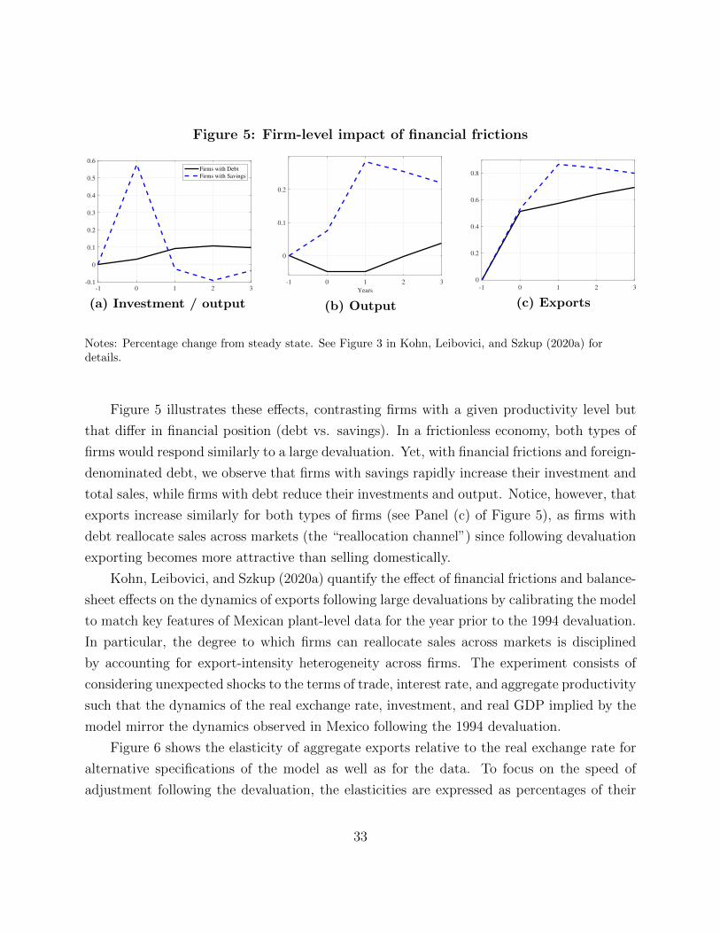
Figure 5: Firm-level impact of financial frictions
-1 0 1 2 3-0.1
0
0.1
0.2
0.3
0.4
0.5
0.6
Firms with Debt
Firms with Savings
(a) Investment / output
-1 0 1 2 3
Years
0
0.1
0.2
(b) Output
-1 0 1 2 3
0
0.2
0.4
0.6
0.8
(c) Exports
Notes: Percentage change from steady state. See Figure 3 in Kohn, Leibovici, and Szkup (2020a) fordetails.
Figure 5 illustrates these effects, contrasting firms with a given productivity level but
that differ in financial position (debt vs. savings). In a frictionless economy, both types of
firms would respond similarly to a large devaluation. Yet, with financial frictions and foreign-
denominated debt, we observe that firms with savings rapidly increase their investment and
total sales, while firms with debt reduce their investments and output. Notice, however, that
exports increase similarly for both types of firms (see Panel (c) of Figure 5), as firms with
debt reallocate sales across markets (the “reallocation channel”) since following devaluation
exporting becomes more attractive than selling domestically.
Kohn, Leibovici, and Szkup (2020a) quantify the effect of financial frictions and balance-
sheet effects on the dynamics of exports following large devaluations by calibrating the model
to match key features of Mexican plant-level data for the year prior to the 1994 devaluation.
In particular, the degree to which firms can reallocate sales across markets is disciplined
by accounting for export-intensity heterogeneity across firms. The experiment consists of
considering unexpected shocks to the terms of trade, interest rate, and aggregate productivity
such that the dynamics of the real exchange rate, investment, and real GDP implied by the
model mirror the dynamics observed in Mexico following the 1994 devaluation.
Figure 6 shows the elasticity of aggregate exports relative to the real exchange rate for
alternative specifications of the model as well as for the data. To focus on the speed of
adjustment following the devaluation, the elasticities are expressed as percentages of their
33

Figure 6: Elasticity of exports to real exchange rate
-1 0 1 2 3
Years
0
0.5
1
Baseline
One type
No reallocation
Data
Notes: Elasticities for each model and the data expressed as a percent of their long-run values. See Figure4 in Kohn, Leibovici, and Szkup (2020a) for details.
final steady-state values. The main finding is that financial frictions and balance-sheet effects
only explain a modest fraction of the slow response of exports observed in the data. This
is primarily accounted for by the reallocation channel: given that exporters typically only
export a small fraction of their total sales, they can substantially increase their exports by
reallocating sales across markets even if severely affected by financial frictions and balance-
sheet effects.
To illustrate the importance of the reallocation channel, Kohn, Leibovici, and Szkup
(2020a) recompute the experiment under two alternative environments. First, they show
that an economy in which this channel is shut down implies a response of exports much
closer to the one observed in the data. Second, they show that an economy estimated to
target the low median export intensity observed in the data, rather than additional features
of the export intensity distribution, features an even faster adjustment of exports than in
the baseline model.
A key take-away message of this paper is that the dynamics of aggregate exports in
economies with financial frictions hinge on firms’ ability to reallocate sales across markets.
34

In Kohn, Leibovici, and Szkup (2020a), reallocating sales is costless and, thus, exports adjust
rapidly despite financial constraints. To the extent that firms actually face reallocation costs,
either because exports are more finance intensive (as in Manova 2013, Chaney 2016, or Kohn,
Leibovici, and Szkup 2016) or because it is costly to adapt goods for different destination
markets, financial frictions and balance-sheet effects are likely to have a stronger impact on
the dynamics of aggregate exports.31
4.3.2 Trade liberalization and financial development
Another important question is whether frictions in financial markets affect the gains from
trade liberalization. Caggese and Cunat (2013) and Kohn, Leibovici, and Szkup (2016) study
partial equilibrium frameworks to analyze how financial development affects the gains from
lowering export barriers. Using Italian and Chilean data, respectively, these studies find that
trade liberalization in the presence of financial frictions leads to a 25% lower increase in TFP
and 18% lower increase in exports, respectively, than in their absence. Both studies find that
financial frictions reduce the gains from trade primarily by distorting the extensive margin
of trade. While informative about industry-level effects, the partial equilibrium nature of
the analysis is a limitation for the study of aggregate effects.
Brooks and Dovis (2020) consider a general equilibrium model based on Melitz (2003) to
investigate how financial frictions affect the gains from bilateral trade liberalization.32 They
find the impact of financial frictions on the gains from trade depends on the type of frictions
that firms face. On the one hand, they find that backward-looking collateral constraints
lead to lower welfare gains than an economy with perfect credit markets. In contrast, they
find that forward-looking constraints do not affect the gains from trade liberalization. Lower
trade barriers increases the future profits of exporters, relaxing their financial constraints
upon trade liberalization — a channel that is absent in economies with backward-looking
collateral constraints.
The above papers do not differentiate between trade in consumption, intermediate, and
capital goods. However, Amiti and Konings (2007), Wacziarg and Welch (2008), and others
document that a key channel through which trade liberalization promotes growth is reduc-
31A separate but related literature investigates the impact of exchange rate volatility on trade (see, forexample, Hericourt and Poncet 2015 and Lin, Shi, and Ye 2018).
32More generally, Bai, Jin, and Lu (2019) and Berthou, Chung, Manova, and Sandoz (2020) study the roleof misallocation in trade liberalization.
35

tions in the costs of importing capital and intermediate inputs. Since financial frictions slow
down capital accumulation, they might particularly affect the gains from trade liberalization
of intermediates and capital goods.
Kohn, Leibovici, and Szkup (2020b) investigate this possibility empirically and quan-
titatively. First, they document that following a reduction in import tariffs on capital and
intermediate inputs, financially developed economies grow faster than less-developed ones.
Then, they study the extent to which this differential impact of trade liberalization is ac-
counted by financial frictions, and investigate their distributional and welfare implications.
To do so, they use an extension of the model from Section 3.1 featuring trade in intermediate
and capital goods. In particular, there are two types of final good composites: a consumption
good and an investment good, each produced by competitive firms that aggregate domestic
and imported varieties. The consumption good is consumed by individuals, while the invest-
ment good is used either for producing capital or as an intermediate input in the production
of domestic varieties. Importantly, varieties imported for the production of consumption or
investment-intermediate goods are subject to tariffs that can be potentially different.
Similarly to the baseline model, firms now face the following financial constraint:
Pk,tki,t+1 ≤1 + r
1 + r − θai,t+1, (13)
where Pk,t is the price of capital goods. This constraint limits the current value of next
period’s capital stock to be lower than a multiple of the firm’s net worth in period t + 1.
Note that the tightness of the borrowing constraint is increasing in the price of capital.33
In this model, reducing tariffs on imported varieties for the production of capital and
intermediate goods has three effects. First, lower tariffs reduce the price of these imported
varieties, increasing imports partially at the expense of domestic varieties. Second, lower
tariffs lead to cheaper investment goods, decreasing the cost of production and investment
while relaxing the borrowing constraints. Finally, lower tariffs lead to real exchange rate
depreciation, increasing the foreign demand for domestic varieties.
Kohn, Leibovici, and Szkup (2020b) calibrate the model using Colombian data (see
Roberts and Tybout 1997) and investigate the effect of reducing import tariffs on capital
goods and intermediates, as implemented in Colombia over 1988-1992. They find that ag-
33If Pk,t = 1 then Equation 13 simplifies to Equation 6.
36

Figure 7: Transition dynamics following a reduction in capital tariffs
5 10 15 20 25 30 35 400
0.005
0.01
0.015
0.02
0.025
0.03
0.035
0.04
Baseline
Financially Developed
(a) Real GDP
5 10 15 20 25 30 35 40
0
0.01
0.02
0.03
0.04
0.05
0.06
0.07
0.08
(b) Capital
5 10 15 20 25 30 35 40
-0.01
0
0.01
0.02
0.03
0.04
(c) Consumption
Source: Kohn, Leibovici, and Szkup (2020b). See the paper for further details.
gregate output, consumption, and capital increase slower than in a financially developed
economy (i.e., an economy in which borrowing constraints are calibrated to match the av-
erage credit-to-GDP ratio across OECD economies), as shown in Figure 7. Moreover, they
show that these findings are consistent with cross-country evidence.
The slower adjustment following trade liberalization reduces the welfare gains from trade
liberalization: these are 0.16% in consumption-equivalence units relative to 0.86% in the
financially developed economy. Moreover, they show that if the economies could transition
to the final steady state immediately, then the welfare gains would be not only larger in
both economies but also very similar. Thus, they conclude that the difference in welfare
gains between the two economies is accounted for by the faster transition in the financially
developed economy. Finally, they show that financial frictions also distort the distributional
effects of trade liberalization: financial frictions increase the concentration of the gains from
trade among rich entrepreneurs, while these gains are more uniformly distributed in the
financially developed economy.34
34Lanteri, Medina, and Tan (2020) emphasize that slow adjustments to an increase in import competitioncan be driven by capital-reallocation frictions. In the presence of such frictions, firms postpone their capitaladjustment choices, which results in a gradual adjustment towards the new steady state.
37

5 Financial frictions and trade: Additional channels
The previous sections summarize a growing literature that investigates the impact of credit
market frictions on firms’ export decisions. Our presentation throughout inevitably required
us to abstract from some channels related to the interaction between trade and finance that
might be important but which would have taken us beyond the scope of this paper. In this
section, we briefly describe some of these channels and the related studies.
Trade finance Recent studies have investigated the determinants of alternative payment
arrangements observed in international trade transactions. Sometimes importers pay for
goods before exporters ship the goods internationally; other times they pay for them after
the goods arrive at the destination. Sometimes these payments are intermediated by banks
through letters of credit; other times they are paid for directly by the parties involved.
Understanding the determinants of these alternative arrangements and the role of finan-
cial constraints has been recently investigated empirically and theoretically by Ahn (2020),
Schmidt-Eisenlohr (2013), Antras and Foley (2015), and Demir and Javorcik (2018), among
others. The studies reviewed in this paper abstract from these channels and instead focus
on the extent to which firms engaged in international trade are more finance intensive and
how this affects firms’ export decisions and other aggregate outcomes.
Financial institutions Another complementary literature has focused on understanding
the role of banks in international trade. This literature is particularly complementary to
the aforementioned studies on trade finance, providing a more focused analysis on the role
played by banks in promoting or hindering international trade transactions. For recent
studies in this literature, see Engemann, Eck, and Schnitzer (2014), Paravisini, Rappoport,
and Schnabl (2015), Niepmann and Schmidt-Eisenlohr (2017a,b), Caballero, Candelaria, and
Hale (2018), and Claessens and Van Horen (2021), among others.35 The studies reviewed in
this paper abstract from the role of banks and, instead, take credit constraints as given and
examine their impact on firms’ production and export decisions.
35For a recent study on the impact of banking crises on exports, see Iacovone, Ferro, Pereira-Lopez, andZavacka (2019).
38

Pattern and logistics of trade Credit market frictions have also been documented to
impact various additional dimensions of the pattern and logistics of international trade trans-
actions. For instance, Chan and Manova (2015) show that financial frictions distort the
choice of trade partners. Relatedly, financial frictions determine whether firms use trade in-
termediaries (Chan 2019) and whether they engage in ordinary or processing trade (Manova
and Yu 2016). These additional dimensions complement those reviewed in this paper, and
are likely to further amplify the distortionary impact of financial frictions on international
trade.
Innovation Another channel through which frictions in financial markets affect interna-
tional trade is by distorting firms’ technology and innovation decisions, as documented by
Egger and Keuschnigg (2015), Foellmi, Legge, and Tiemann (2015), and Faustino and Matos
(2015). To the extent that exporting is dependent on innovation, the finance-intensive nature
of R&D and innovation activities implies that this channel may amplify the distortionary
impact of credit market frictions. Indeed, Bonfiglioli, Crino, and Gancia (2019) show that fi-
nancial frictions can discourage entering firms from investing in risky but innovative projects.
In a similar spirit, Foellmi and Oechslin (2020) show that in the presence of financial frictions,
opening to trade may force firms to switch to less productive (traditional) technologies.
Multinational firms Multinational firms have long been documented to serve as an ad-
ditional source of finance in economies with underdeveloped financial markets (Desai, Foley,
and Forbes 2008). In particular, multinational firms are typically considered to be less sub-
ject to credit constraints faced by host countries since they can also access foreign sources of
capital. Manova, Wei, and Zhang (2015) show that the financial advantages of multinational
firms play an important role in shaping the patterns of both international trade and multi-
national activity. Spencer (2020) develops a quantitative model with firm heterogeneity and
financial frictions to study the impact of corporate tax reforms targeted at multinationals.
6 Concluding remarks
This paper reviews recent studies on the impact of financial frictions on international trade,
a literature that has grown rapidly following the global financial crisis of 2008-2009. A
39

wide range of studies shows that financial factors are not only important determinants of
macroeconomic outcomes but also important determinants of international trade decisions.
Yet, much work remains to be done to sharpen our understanding of the channels through
which credit market frictions affect international trade and these frictions’ implications for
aggregate outcomes. Data availability has been a key limiting factor for the progress of this
area of research.
First, while much of the literature has investigated the determinants of firms’ export
decisions using manufacturing surveys, these have typically failed to systematically collect
the detailed financial information required to deepen our understanding of the impact of
financial channels on real outcomes. Improved collection of firm-level financial information
that can be linked to real outcomes at higher frequencies and with broader sectoral coverage
will help advance our understanding of the channels discussed in this paper.
Second, limited data availability on importers has likely amplified the literature’s focus
on understanding firms’ export decisions. The result has been a more limited understanding
of importers and the role that financial factors may play in accounting for their choices. As
new and more detailed firm-level datasets become available, we might have a more compre-
hensive picture of the role of financial factors along this margin.
Third, increased data availability across countries is also likely to spur the growth of
related areas of research. For instance, with the increased growth of global value chains
and their importance for international trade, financial shocks in a location are increasingly
likely to be transmitted across countries. Thus, the trade-finance nexus is likely to be
an increasingly important channel for the transmission of financial shocks across countries,
raising novel questions on the design of trade and financial policies. We expect the present
review to serve researchers and practitioners alike as a starting point to conduct further
research and design policies to address these and other important questions about the link
between trade and finance.
Finally, a better understanding of the trade-finance nexus holds the promise of improving
our knowledge of how financial frictions affect economic outcomes more broadly. In some
respects, trade data is richer and more systematically collected than data on firms’ domestic
transactions and operations. Thus, this line of research has the potential to shed light on
key aspects of financial market frictions.
40

References
Aguiar, M. (2005): “Investment, devaluation, and foreign currency exposure: The case of Mex-ico,” Journal of Development Economics, 78, 95–113.
Aguirre, A., M. Tapia, and L. Villacorta (2021): “Production, Investment and WealthDynamics under Financial Frictions: An Empirical Investigation of the Self-financing Channel,”Central Bank of Chile, Working paper No. 904.
Ahn, J. (2020): “A Theory of Domestic and International Trade Finance,” Emerging MarketFinance: New Challenges and Opportunities (International Finance Review, Vol. 21).
(2021): “Trade Finance and Payment Methods in International Trade,” Working paper.Albornoz, F., H. F. C. Pardo, G. Corcos, and E. Ornelas (2012): “Sequential exporting,”
Journal of International Economics, 88(1), 17–31.Albuquerque, R., and H. A. Hopenhayn (2004): “Optimal lending contracts and firm dynam-
ics,” The Review of Economic Studies, 71(2), 285–315.Alessandria, G., C. Arkolakis, and K. J. Ruhl (2021): “Firm dynamics and trade,” Annual
Review of Economics, 13.Alessandria, G., and O. Avila (2020): “Trade Integration in Colombia: A Dynamic General
Equilibrium Study with New Exporter Dynamics,” Journal of Economic Dynamics and Control,115, 103871.
Alessandria, G., and H. Choi (2007): “Do Sunk Costs of Exporting Matter for Net ExportDynamics?,” The Quarterly Journal of Economics, 122(1), 289–336.
(2014a): “Do falling iceberg costs explain recent US export growth?,” Journal of Inter-national Economics, 94(2), 311–325.
(2014b): “Establishment Heterogeneity, Exporter Dynamics, and the Effects of TradeLiberalization,” Journal of International Economics, 94(2), 207–223.
Alessandria, G., H. Choi, and K. J. Ruhl (2021): “Trade adjustment dynamics and thewelfare gains from trade,” Journal of International Economics, 131, 103458.
Alessandria, G., S. Pratap, and V. Z. Yue (2014): “Export dynamics in large devaluations,”Working paper.
Amiti, M., and J. Konings (2007): “Trade liberalization, intermediate inputs, and productivity:Evidence from Indonesia,” American Economic Review, 97(5), 1611–1638.
Amiti, M., and D. Weinstein (2011): “Exports and Financial Shocks,” The Quarterly Journalof Economics, 126(4), 1841–1877.
Andreasen, E., S. Bauducco, and E. Dardati (2019): “Capital Controls and Firm Perfor-mance,” Discussion paper, Central Bank of Chile.
Antras, P., and R. J. Caballero (2009): “Trade and capital flows: A financial frictionsperspective,” Journal of Political Economy, 117(4), 701–744.
Antras, P., and C. F. Foley (2015): “Poultry in motion: A study of international trade financepractices,” Journal of Political Economy, 123(4), 853–901.
Arellano, C., Y. Bai, and J. Zhang (2012): “Firm Dynamics and Financial Development,”Journal of Monetary Economics, 59(6), 533–549.
41

Arkolakis, C. (2010): “Market Penetration Costs and the New Consumers Margin in Interna-tional Trade,” Journal of Political Economy, 118(6).
Bai, Y., K. Jin, and D. Lu (2019): “Misallocation under trade liberalization,” Discussion paper,National Bureau of Economic Research.
Baldwin, R., and P. Krugman (1989): “Persistent trade effects of large exchange rate shocks,”The Quarterly Journal of Economics, 104(4), 635–654.
Beck, T. (2002): “Financial Development and International Trade: Is There a Link?,” Journal ofInternational Economics, 57(1), 107–131.
(2003): “Financial Dependence and International Trade,” Review of International Eco-nomics, 11(2), 296–316.
Beck, T., A. Demirguc-Kunt, and R. Levine (2010): “Financial institutions and marketsacross countries and over time: The updated financial development and structure database,”The World Bank Economic Review, 24(1), 77–92.
Bellone, F., P. Musso, L. Nesta, and S. Schiavo (2010): “Financial Constraints and FirmExport Behaviour,” The World Economy, 33(3), 347–373.
Bergin, P., L. Feng, and C.-Y. Lin (2018a): “Financial frictions and trade dynamics,” IMFEconomic Review, 66(3), 480–526.
(2018b): “Firm entry and financial shocks,” The Economic Journal, 128(609), 510–540.Bergin, P. R., L. Feng, and C.-Y. Lin (2021): “Trade and firm financing,” Journal of Inter-
national Economics, 131, 103461.Berman, N., and A. Berthou (2009): “Financial market imperfections and the impact of ex-
change rate movements on exports,” Review of International Economics, 17(1), 103–120.Berman, N., A. Berthou, and J. Hericourt (2015): “Export dynamics and sales at home,”
Journal of International Economics, 96(2), 298–310.Berman, N., and J. Hericourt (2010): “Financial factors and the margins of trade: Evidence
from cross-country firm-level data,” Journal of Development Economics, 93(2), 206–217.(2011): “Debt denomination, exchange-rate variations and the margins of trade,” Applied
Economics Letters, 18(9), 817–822.Bernanke, B. S., M. Gertler, and S. Gilchrist (1999): “The financial accelerator in a
quantitative business cycle framework,” Handbook of Macroeconomics, 1, 1341–1393.Berthou, A., J. J.-H. Chung, K. Manova, and C. Sandoz (2020): “Trade, Productivity and
(Mis)allocation,” Working paper.Bilir, L. K., D. Chor, and K. Manova (2019): “Host-country financial development and
multinational activity,” European Economic Review, 115, 192–220.Bonfiglioli, A., R. Crino, and G. Gancia (2019): “Trade, finance, and endogenous firm
heterogeneity,” Journal of the European Economic Association, 17(1), 79–130.Brooks, W., and A. Dovis (2020): “Credit market frictions and trade liberalizations,” Journal
of Monetary Economics, 111, 32–47.Buera, F. J., J. P. Kaboski, and Y. Shin (2011): “Finance and Development: A Tale of Two
Sectors,” American Economic Review, 101(5), 1964–2002.Buera, F. J., J. P. Kaboski, and Y. Shin (2015): “Entrepreneurship and financial frictions:
A macrodevelopment perspective,” Annual Reviews of Economics, 7(1), 409–436.
42

Buera, F. J., and B. Moll (2015): “Aggregate Implications of a Credit Crunch,” AmericanEconomic Journal: Macro, 7.
Buera, F. J., and Y. Shin (2013): “Financial frictions and the persistence of history: A quanti-tative exploration,” Journal of Political Economy, 121(2), 221–272.
(2017): “Productivity growth and capital flows: The dynamics of reforms,” AmericanEconomic Journal: Macroeconomics, 9(3), 147–85.
Caballero, J., C. Candelaria, and G. Hale (2018): “Bank linkages and international trade,”Journal of International Economics, 115, 30–47.
Caggese, A., and V. Cunat (2013): “Financing Constraints, Firm Dynamics, Export Decisions,and Aggregate Productivity,” Review of Economic Dynamics, 16(1), 177–193.
Chan, J. M. (2019): “Financial frictions and trade intermediation: Theory and evidence,” Euro-pean Economic Review, 119, 567–593.
Chan, J. M., and K. Manova (2015): “Financial development and the choice of trade partners,”Journal of Development Economics, 116, 122–145.
Chaney, T. (2008): “Distorted Gravity: The Intensive and Extensive Margins of InternationalTrade,” American Economic Review, 98(4), 1707–1721.
(2016): “Liquidity constrained exporters,” Journal of Economic Dynamics and Control,72, 141–154.
Claessens, S., and N. Van Horen (2021): “Foreign banks and trade,” Journal of FinancialIntermediation, 45, 100856.
Clementi, G. L., and H. A. Hopenhayn (2006): “A Theory of Financing Constraints and FirmDynamics,” Quarterly Journal of Economics, 121(1), 229–265.
Contessi, S., and F. De Nicola (2012): “What do we know about the relationship betweenaccess to finance and international trade?,” Federal Reserve Board of St. Louis working paper2012-054B.
Cooley, T., and V. Quadrini (2001): “Financial Markets and Firm Dynamics,” AmericanEconomic Review, 91(5).
Das, S., M. J. Roberts, and J. R. Tybout (2007): “Market entry costs, producer heterogeneity,and export dynamics,” Econometrica, 75(3), 837–873.
Demir, B., and B. Javorcik (2018): “Don’t throw in the towel, throw in trade credit!,” Journalof International Economics, 111, 177–189.
Desai, M. A., C. F. Foley, and K. J. Forbes (2008): “Financial constraints and growth:Multinational and local firm responses to currency depreciations,” Review of Financial Studies,21(6), 2857–2888.
Dixit, A. (1989): “Hysteresis, import penetration, and exchange rate pass-through,” The Quar-terly Journal of Economics, 104(2), 205–228.
Djankov, S., C. Freund, and C. S. Pham (2010): “Trading on Time,” The Review of Economicsand Statistics, 92(1), 166–173.
Eaton, J., M. Eslava, D. Jinkins, C. J. Krizan, and J. Tybout (2014): “A Search andLearning Model of Export Dynamics,” Working paper.
Edwards, S. (1986): “Are Devaluations Contractionary?,” The Review of Economics and Statis-tics, 68(3), 501–508.
43

Egger, P., and M. Kesina (2013): “Financial Constraints and Exports: Evidence from ChineseFirms,” CESifo Economic Studies, 59(4), 676–706.
Egger, P., and C. Keuschnigg (2015): “Innovation, trade, and finance,” American EconomicJournal: Microeconomics, 7(2), 121–57.
Engemann, M., K. Eck, and M. Schnitzer (2014): “Trade credits and bank credits in inter-national trade: Substitutes or complements?,” The World Economy, 37(11), 1507–1540.
Estevadeordal, A., and A. M. Taylor (2013): “Is the Washington consensus dead? Growth,openness, and the great liberalization, 1970s–2000s,” Review of Economics and Statistics, 95(5),1669–1690.
Faustino, H. C., and P. V. Matos (2015): “Exports, productivity and innovation: New firmlevel empirical evidence,” Applied Economics, 47(46), 4918–4933.
Feenstra, R. C., R. Inklaar, and M. P. Timmer (2015): “The next generation of the PennWorld Table,” American Economic Review, 105(10), 3150–82.
Feenstra, R. C., M. Yu, and Z. Li (2014): “Exports and Credit Constraints under IncompleteInformation: Theory and Evidence from China,” The Review of Economics and Statistics, 96(4),729–744.
Fitzgerald, D., S. Haller, and Y. Yedid-Levi (2016): “How exporters grow,” Workingpaper.
Foellmi, R., S. Legge, and A. Tiemann (2015): “Innovation and trade in the presence of creditconstraints,” Working paper.
Foellmi, R., and M. Oechslin (2020): “Harmful procompetitive effects of trade in presence ofcredit market frictions,” Journal of Money, Credit and Banking, 52(6), 1493–1525.
Foley, C. F., and K. Manova (2015): “International Trade, Multinational Activity, and Cor-porate Finance,” Annual Review of Economics, 7(1), 119–146.
Francis, D. C., N. Karalashvili, H. Maemir, and J. Rodriguez Meza (2020): “MeasuringTotal Factor Productivity Using the Enterprise Surveys,” Working paper.
Frankel, J. A. (2005): “Mundell-Fleming Lecture: Contractionary Currency Crashes in Devel-oping Countries,” IMF Staff Papers, pp. 149–192.
Frankel, J. A., and D. H. Romer (1999): “Does trade cause growth?,” American economicreview, 89(3), 379–399.
Friedrich, B. U., and M. Zator (2021): “Flexibility costs of debt: Danish exporters duringthe cartoon crisis,” Working paper.
Gopinath, G., S. Kalemli-Ozcan, L. Karabarbounis, and C. Villegas-Sanchez (2017):“Capital allocation and productivity in South Europe,” The Quarterly Journal of Economics,132(4), 1915–1967.
Greenaway, D., A. Guariglia, and R. Kneller (2007): “Financial factors and exportingdecisions,” Journal of International Economics, 73, 377–395.
Gross, T., and S. Verani (2013): “Financing Constraints, Firm Dynamics, and InternationalTrade,” FRB, Finance and Economics Discussion Series.
Hericourt, J., and S. Poncet (2015): “Exchange rate volatility, financial constraints, and trade:Empirical evidence from Chinese firms,” The World Bank Economic Review, 29(3), 550–578.
44
Hur, J., M. Raj, and Y. E. Riyanto (2006): “Finance and trade: A cross-country empiricalanalysis on the impact of financial development and asset tangibility on international trade,”World Development, 34(10), 1728–1741.
Iacovone, L. (2008): “Exploring Mexican firm-level data,” University of Sussex.Iacovone, L., E. Ferro, M. Pereira-Lopez, and V. Zavacka (2019): “Banking crises and
exports: lessons from the past,” Journal of Development Economics, 138, 192–204.Kalemli-Ozcan, S., H. Kamil, and C. Villegas-Sanchez (2016): “What Hinders Investment
in the Aftermath of Financial Crises: Insolvent Firms or Illiquid Banks?,” Review of Economicsand Statistics, 98(4), 756–769.
Kiyotaki, N., and J. Moore (1997): “Credit cycles,” Journal of Political Economy, 105(2),211–248.
Kohn, D., F. Leibovici, and M. Szkup (2016): “Financial Frictions and New Exporter Dynam-ics,” International Economic Review, 57(2), 453–486.
(2017): “Financial frictions, trade, and misallocation,” Working paper.(2020a): “Financial frictions and export dynamics in large devaluations,” Journal of
International Economics, 122, 103257.(2020b): “No Credit, No Gain: Trade Liberalization Dynamics, Production Inputs, and
Financial Development,” Working paper.Krueger, A. O. (1997): “Trade Policy and Economic Development: How We Learn,” American
Economic Review, 87(1), 1–22.Lanteri, A., P. Medina, and E. Tan (2020): “Capital-reallocation frictions and trade shocks,”
Working paper.Leibovici, F. (2021): “Financial Development and International Trade,” Journal of Political
Economy, 129(12), 3405–3446.Lin, S., K. Shi, and H. Ye (2018): “Exchange rate volatility and trade: The role of credit
constraints,” Review of Economic Dynamics, 30, 203–222.Manova, K. (2013): “Credit Constraints, Heterogeneous Firms, and International Trade,” Review
of Economic Studies, 80(2), 711–744.Manova, K., S.-J. Wei, and Z. Zhang (2015): “Firm exports and multinational activity under
credit constraints,” Review of Economics and Statistics, 97(3), 574–588.Manova, K., and Z. Yu (2016): “How firms export: Processing vs. ordinary trade with financial
frictions,” Journal of International Economics, 100, 120–137.Matsuyama, K. (2004): “Financial market globalization, symmetry-breaking, and endogenous
inequality of nations,” Econometrica, 72(3), 853–884.(2005): “Credit market imperfections and patterns of international trade and capital
flows,” Journal of the European Economic Association, 3(2-3), 714–723.Melitz, M. J. (2003): “The Impact of Trade on Intra-Industry Reallocations and Aggregate
Industry Productivity,” Econometrica, 71(6), 1695–1725.Midrigan, V., and D. Y. Xu (2014): “Finance and Misallocation: Evidence from Plant-Level
Data,” American Economic Review, 104(2), 422–58.Minetti, R., and S. Zhu (2011): “Credit Constraints and Firm Export: Microeconomic Evidence
from Italy,” Journal of International Economics, 83(2), 1695–1725.
45

Moll, B. (2014): “Productivity Losses from Financial Frictions: Can Self-Financing Undo CapitalMisallocation?,” American Economic Review, 104(10), 3186–3221.
Muuls, M. (2015): “Exporters, importers and credit constraints,” Journal of International Eco-nomics, 95(2), 333–343.
Nguyen, D. X. (2012): “Demand uncertainty: Exporting delays and exporting failures,” Journalof International Economics, 86(2), 336–344.
Niepmann, F., and T. Schmidt-Eisenlohr (2017a): “International trade, risk and the role ofbanks,” Journal of International Economics, 107, 111–126.
(2017b): “No guarantees, no trade: How banks affect export patterns,” Journal of Inter-national Economics, 108, 338–350.
Paravisini, D., V. Rappoport, and P. Schnabl (2015): “Specialization in bank lending:Evidence from exporting firms,” Discussion paper, National Bureau of Economic Research.
Paravisini, D., V. Rappoport, P. Schnabl, and D. Wolfenzon (2015): “Dissecting theeffect of credit supply on trade: Evidence from matched credit-export data,” The Review ofEconomic Studies, 82(1), 333–359.
Rajan, R. G., and L. Zingales (1998): “Financial Dependence and Growth,” American Eco-nomic Review, 88(3), 559–586.
Rho, Y., and J. Rodrigue (2016): “Firm-level investment and export dynamics,” InternationalEconomic Review, 57(1), 271–304.
Roberts, M. J., and J. R. Tybout (1997): “The Decision to Export in Colombia: An EmpiricalModel of Entry with Sunk Costs,” American Economic Review, 87(4), 545–564.
Ruhl, K. J., and J. L. Willis (2017): “New exporter dynamics,” International Economic Review,58(3), 703–726.
Schmidt-Eisenlohr, T. (2013): “Towards a theory of trade finance,” Journal of InternationalEconomics, 91(1), 96–112.
Spencer, A. (2020): “Policy effects of international taxation on firm dynamics and capital struc-ture,” Available at SSRN 2742006.
Svaleryd, H., and J. Vlachos (2005): “Financial markets, the pattern of industrial specializa-tion and comparative advantage: Evidence from OECD countries,” European Economic Review,49(1), 113–144.
Tauchen, G. (1986): “Finite state Markov-chain approximations to univariate and vector autore-gressions,” Economics letters, 20(2), 177–181.
Tetenyi, L. (2019): “Trade, misallocation, and capital market integration,” Working paper.The World Bank (2021): “Enterprise Surveys,” http://www.enterprisesurveys.org.Vaubourg, A.-G. (2016): “Finance and international trade: A review of the literature,” Revue
d’economie politique, 126(1), 57–87.Wacziarg, R., and K. H. Welch (2008): “Trade liberalization and growth: New evidence,”
The World Bank Economic Review, 22(2), 187–231.
46

Appendix
Appendix A Summary statistics
Table 4 reports summary statistics for each of the variables analyzed in Section 2. We restrict
attention to summary statistics after aggregating the firm-level information to the country
level. The ratio of exports to total sales and TFP is averaged across all firms within each
country, and the FP reports the share of firms in each country that report finance to be a
problem as defined above.
We observe substantial heterogeneity across countries in exporting performance. While
the average share of exporters across countries is 29%, the 25th and 75th percentiles vary
widely: 16% and 37%, respectively. We find that exporters in most countries tend to sell a
significant fraction abroad on average. The average share of production that exporters sell
abroad is 46%, with the 25th and 75th percentiles ranging from 36% to 53%.
Similarly, we observe substantial heterogeneity in financial development across countries
according to both the share of firms that report finance to be a problem and from the lens
of the aggregate credit-to-GDP ratio. On average, 49% of all firms report finance to be
a problem, with the 25th and 75th percentiles ranging from 39% to 59%. The credit-to-
GDP ratio is 41% on average, with the corresponding percentiles range from 17% to 56%,
respectively.
Appendix B Calibration
In this section we describe the calibration underlying the figures presented in Section 3.2. We
calibrate the model with financial frictions following Kohn, Leibovici, and Szkup (2020a).
We partition the parameter space into two groups. The parameters in the first group are set
to values commonly used in the literature, as reported in Panel A of Table 5.
The parameters in the second group are the iceberg trade cost τ , fixed cost of exporting
F , persistence of productivity shocks ρ, standard deviation of productivity shocks σε, and
the tightness of the financial constraint θ. We choose them to match the following moments:
(i) the average export intensity (i.e., the average share of export sales in total sales), (ii)
the share of exporters, (iii) the share of sales accounted by the largest 25% of firms, (iv) the
47
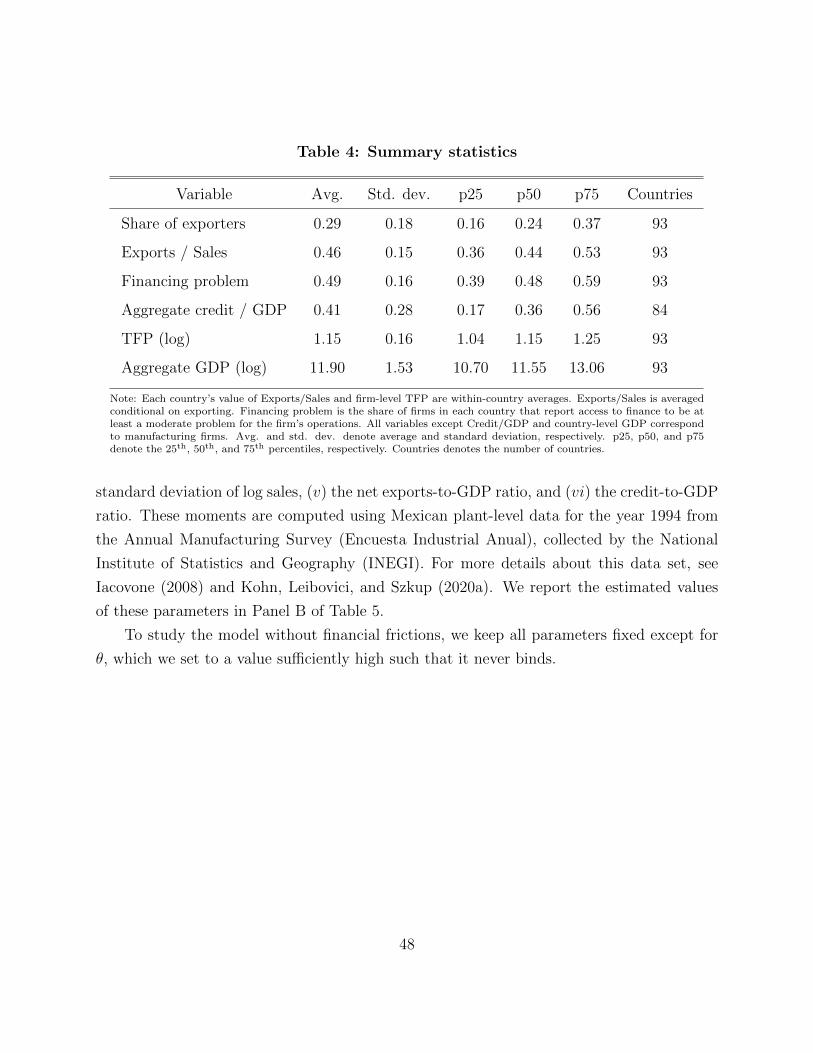
Table 4: Summary statistics
Variable Avg. Std. dev. p25 p50 p75 Countries
Share of exporters 0.29 0.18 0.16 0.24 0.37 93
Exports / Sales 0.46 0.15 0.36 0.44 0.53 93
Financing problem 0.49 0.16 0.39 0.48 0.59 93
Aggregate credit / GDP 0.41 0.28 0.17 0.36 0.56 84
TFP (log) 1.15 0.16 1.04 1.15 1.25 93
Aggregate GDP (log) 11.90 1.53 10.70 11.55 13.06 93
Note: Each country’s value of Exports/Sales and firm-level TFP are within-country averages. Exports/Sales is averagedconditional on exporting. Financing problem is the share of firms in each country that report access to finance to be atleast a moderate problem for the firm’s operations. All variables except Credit/GDP and country-level GDP correspondto manufacturing firms. Avg. and std. dev. denote average and standard deviation, respectively. p25, p50, and p75denote the 25th, 50th, and 75th percentiles, respectively. Countries denotes the number of countries.
standard deviation of log sales, (v) the net exports-to-GDP ratio, and (vi) the credit-to-GDP
ratio. These moments are computed using Mexican plant-level data for the year 1994 from
the Annual Manufacturing Survey (Encuesta Industrial Anual), collected by the National
Institute of Statistics and Geography (INEGI). For more details about this data set, see
Iacovone (2008) and Kohn, Leibovici, and Szkup (2020a). We report the estimated values
of these parameters in Panel B of Table 5.
To study the model without financial frictions, we keep all parameters fixed except for
θ, which we set to a value sufficiently high such that it never binds.
48

Table 5: Parameterization for Section 3
Panel A: Predetermined parameters
Parameter Value Description
γ 2 Risk aversion
σ 4 Elasticity of substitution
δ 0.06 Capital depreciation rate
r 0.08 Interest rate
α 0.33 Capital share
pm 1 Price imports
Yf 10 Rest of the world aggregate demand
Panel B: Estimated parameters
Parameter Value Target moment Data Model
τ 5.18 Export intensity 0.23 0.23
F 0.07 Share of exporters 0.32 0.32
ρ 0.89 Share of sales accounted by top 25% 0.84 0.84
σε 0.24 Standard deviation of log sales 1.52 1.52
β 0.84 Net exports / GDP -0.03 -0.03
θ 0.21 Credit / GDP 0.44 0.44
Note: The parameters reported in this table are used to compute the results for the financial-frictions modelreported in Figures 1 and 2 of the paper.
49