financial development and economic growth …621160/fulltext… · · 2013-05-13financial...
TRANSCRIPT

1
FINANCIAL DEVELOPMENT AND ECONOMIC GROWTH
-An Empirical Investigation of the nexus in Ghana
Södertörns högskola | Institutionen för Samhällsvetenskaper
Magisteruppsats 30 hp | Nationalekonomi | Vårterminen 2013
Av: Adwoa Dufie Oppong
Handledare: Karl Markus Modén
Opposition: 2013-04-05

2
ACKNOWLEGEMENT
First of all I would like to thank the Almighty God for His immense protection during my time of
study in Sweden. My sincere thanks go to Dr. George Adu (Economics Dept. KNUST) for
providing me with the data and giving me many useful suggestions
I would also like to thank Karl Markus Moden (Sodertorns Hogskola) for supervising my work
Much love to my family and friends back home in Ghana.

3
“...I thought of growth theory as the search for a dynamic model that could explain the evolution
of one economy overtime. There were no explicit cross sectional implications.” Solow (2001)
ABSTRACT
This paper examines the causal relationship between financial development and economic
growth in Ghana. This is done using modern time series econometric procedures by employing
four proxies of financial development and applying Granger causality test, Cointegration and
Vector Error Correction Model (VECM) .The empirical results show that the direction of
causality is sensitive to the choice of proxy of financial development. It was discovered that
finance follows in the direction of economic growth but doesn’t necessarily lead to it. The
empirical Cointegration results weakly support a long run relationship between financial
development and economic growth
Keywords: Financial Development, Economic Growth, Granger Causality, Cointegration

4
CONTENTS
1 INTRODUCTION 5
2 FORMULATING THE PROBLEM 6
3 BACKGROUND 6
3.1 Some Stylized Facts about Growth in Ghana 6
4 THEORY 9
4.1 Financial Development 9
4.2 Economic Growth 10
4.3 Finance versus Growth: The Theoretical Literature 10
5 EARLIER STUDIES 12
6 METHODOLOGY 15
7 DATA 16
8 ECONOMETRIC MODELLING 17
8.1 Model Specification 17
8.2 Empirical Strategy 19
9 RESULTS 23
9.1 Results of the unit root test 23
9.2 Testing for causality: Economic Growth versus Financial Development 23
9.2.1 Growth versus broad money supply 24
9.2.2 Growth versus domestic credit to the private sector 24
9.2.3 Growth versus total domestic credit 24
9.2.4 Growth versus currency to GDP ratio 24
9.3 Investigating the main determinants of growth 25
9.4 The long run relationship between growth and its determinants 25
9.5 The short run relationship (Vector Error Correction Model) 26
10 ANALYSIS 26
11 CONCLUSION 31
12 REFERENCES 33
13 APPENDIX 36

5
1 Introduction
An important statistic for evaluating economic performance for any given economy is its annual
rate of real GDP growth. As a result, there are a large numbers of studies that attempt to identify
the main drivers of economic growth and the potential sources of growth differentials across
space and time from both theoretical and empirical perspectives. This notwithstanding, the
evidence is not conclusive and the debate on whether financial development is the cause of effect
of the growth process is still ongoing. Another source of dispute on this strand of growth
literature is the issue of appropriate or correct measure of financial development. This study aims
to address these concerns in the literature using time series econometric techniques.
The existing literature has identified many transmission channels through which financial
development may impact on economic growth via their effect on savings and investment
behaviour. According to Levine (2004), financial development involves improvements in the (i)
production of information about possible investments, (ii) monitoring of investments and
implementation of corporate governance, (iii) trading, diversification, and management of risk,
(iv) mobilization and pooling of savings, and (v) exchange of goods and services. The financial
functions affect savings and investment and subsequently lead to economic growth.
Since many market frictions exist and since laws, regulations, and policies differ markedly
across economies and overtime, improvements along any single dimension may have different
implications for resource allocation and welfare depending on the other frictions at play in the
economy.
Chapter 3 of the thesis outlines the problem statement. Chapter 4 expresses background
information on financial developments and economic growth. Chapter 5 presents theories.
Earlier studies on this nexus will be briefly reviewed in chapter 6.Chapters 7 and 8 describe the

6
procedure for approaching the objective as well as data used to analyze it. Chapter 9 presents
how the econometric technique will be implemented. The empirical finding will be presented in
chapter 10.Chapter 11 analyses the results.The summary and references are presented in chapters
12 and 13 respectively.
2 Formulating the Problem
The objective of this thesis is to investigate the causal linkage between financial development
and economic growth in Ghana from 1960 to 2010
Research Question
Financial development and Economic Growth;Is there a causality?
3 Background
3.1 Some Stylized Facts about Growth in Ghana
Ghana has tried various approaches to achieve acceptable rates of development and growth since
independence in 1957.A push for rapid industrialization began in the 1960s, using a wide array
of control measures and state interventions. In the 1970s, the interventions continued but with
little indication as to what the ultimate development goals were (Aryeetey, et. al., 2000).
By the beginning of 1983, inappropriate macroeconomic and institutional development policies,
combined with various external shocks, had led to severe deterioration in economic performance.
While the approaches employed in putting economic development concepts into practice have
often been undermined by incompatible socio-political tendencies, the economic policies

7
articulated, have usually been fashioned to achieve internationally acceptable growth rate and
development.
The growth record of Ghana has been one of unevenness when the post reformed period (after
1984) is compared to the earlier period since independence in 1957.With reasonably high GDP
growth in the 1950s and early 1960s, the Ghanaian economy began to experience a slowdown in
GDP growth in 1964.Economic growth in Ghana was turbulent during much of the period after
mid 1960s and only began to stabilize after 1984.In 1966, 1972, 1975-1976,1979,and 1983,the
growth rate of real GDP was negative(see figure 1)
Interestingly, the years which experienced negative growth coincided with changes in
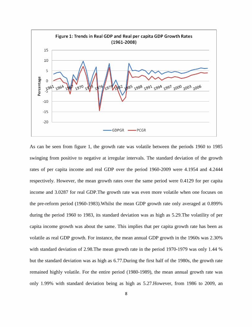
government (political instability) and also policy reversals. Figure 1 shows the trend in the
growth rates of real per capita GDP (PCGR) and real GDP (GDPGR) from 1961 to 2009
inclusive. The stable co-movement of per capita growth indicates that over the period 1961 to
2009, the population growth rate has been constant over the period under study. The growth rates
were highest in 1970 under the second republic constitutional administration headed by Prime
Minister K.A Busia. In 1970, the recorded real GDP growth was 9.72% whilst per capita income
grew at 7.2%. Unfortunately this record level of growth was not sustained following the
February 1972 coup headed by General Acheampong. By 1975, the growth rates of per capita
income and real GDP hit all-time lows of -14.49% and -12.43 % respectively. Growth remained
poor and negative in most of the years from 1972 until reform period in the mid-1980s.
8
As can be seen from figure 1, the growth rate was volatile between the periods 1960 to 1985
swinging from positive to negative at irregular intervals. The standard deviation of the growth
rates of per capita income and real GDP over the period 1960-2009 were 4.1954 and 4.2444
respectively. However, the mean growth rates over the same period were 0.4129 for per capita
income and 3.0287 for real GDP.The growth rate was even more volatile when one focuses on
the pre-reform period (1960-1983).Whilst the mean GDP growth rate only averaged at 0.899%
during the period 1960 to 1983, its standard deviation was as high as 5.29.The volatility of per
capita income growth was about the same. This implies that per capita growth rate has been as
volatile as real GDP growth. For instance, the mean annual GDP growth in the 1960s was 2.30%
with standard deviation of 2.98.The mean growth rate in the period 1970-1979 was only 1.44 %
but the standard deviation was as high as 6.77.During the first half of the 1980s, the growth rate
remained highly volatile. For the entire period (1980-1989), the mean annual growth rate was
only 1.99% with standard deviation being as high as 5.27.However, from 1986 to 2009, an

9
annual growth rate of 5% made it stabilize as can be seen from figure 1.From 1985 to 1989, the
growth rate of real GDP averaged around 5%.Since then, the growth of real GDP has been very
stable at slightly above 4% in the 1990s and 2000s.The above facts about Ghana’s post
independent growth performance calls for a probe into the main drivers of economic growth in
Ghana. In view of the important role that economic growth plays in the development process of
the economy of Ghana, it is important to understand the nature and determinants of economic
growth.
4 Theory
4.1 Financial Development
According to Levine (2004), financial development occurs when financial instruments, markets,
and intermediaries ameliorate though do not necessarily eliminate the effects of information,
enforcement, and transactions cost and therefore perform their core function more effectively.
This implies according to Levine (2004), (i) production of information about possible
investments, (ii) monitoring of investments and implementation of corporate governance, (iii)
trading, diversification and management of risks, (iv) mobilization and pooling of savings, and
(v) exchange of goods and services. The financial functions affect savings and investment and
subsequently lead to economic growth. Since many market imperfections exist and since laws,
regulations, and policies differ markedly across economies and over time, improvements along
any single dimension may have different implications for resource allocation and welfare
depending on other imperfections at play in the economy

10
4.2 Economic Growth
This is generally defined as the percentage change in the real gross domestic product (GDP),
usually on per annum basis. For purposes of international comparison, the per capita GDP
growth is typically used for such purposes. The aim is to adjust for country size, proxy by the
total population of the country. Usually, a distinction is also made between nominal and real
GDP to account for differences in prices across space and time. In this thesis, I measure
economic growth as the annual percentage in Ghana’s real GDP.
4.3 Finance versus Growth: The Theoretical Literature
A large growth accounting literature suggests that physical capital accumulation per se does not
account for much of long run economic growth (Jorgenson, 1995, 2005).Thus, if finance is to
explain economic growth, there should be theories that describe how financial development
influences resource allocation decisions in ways that foster productivity growth and not aim the
analytical spotlight too narrowly on aggregate savings.
There are two general controversies in terms of distinguishing between economic growth and the
emergence of financial arrangements that improve resource allocation and reduce risk.
Specifically, income and substitutions effects make higher returns ambiguously affects savings
rates. According to (Levhari and Srinivasan, 1969), lower risk also ambiguously affects savings
rates. Thus, financial institutions function as improvement in resource allocation and lower risk
may also lower savings rates. Financial development could retard economic growth and lower
welfare if the drop in savings and the externality combine to produce a sufficiently large effect.

11
These controversies are general features of virtually all the models discussed below so I do not
discuss them when describing each model.
Resource allocation is improved when financial intermediaries reduce the costs of acquiring and
processing information (Boyd and Prescott, 1986).Investors would face the large fixed costs
associated with managers, evaluating firms and economic conditions without these
intermediaries.
If groups of individuals form financial intermediaries, the cost of researching investment
possibilities for others may be reduced. Financial intermediaries act like banks by accepting
deposits and making loans (Boyd and Prescott 1986).Models where financial intermediaries arise
to arise to produce information on firms and sell this information to savers were developed by
Ramakrishnan and Thakor (1984),Bhattacharya and Pfeiderer (1985),and Allen (1990)
These intermediaries do not necessarily both mobilize savings and invest those funds in firms
using debt contracts in Boyd and Prescott (1986).Financial intermediaries by economizing on
information acquisition costs improve the ex-ante assessment of investment opportunities with
positive ramifications on resource allocation. Financial intermediaries can accelerate economic
growth by improving information on firms, managers and economic conditions. Taking the
assumption that entrepreneurs solicit for capital and that capital is scarce, financial
intermediaries that produce better information on firms will thereby fund more promising firms
and induce a more efficient allocation of capital (Greenwood and Jovanovic, 1990).
Financial sectors role believed to be growth enhancing from a theoretical perspective is risk
sharing and optimal allocation of capital, risk and returns. The links between cross sectional risk,

12
diversification, and growth was carefully modeled by Acemoglu and Zilibotti (1997) .They
assume that (i) high-return, risky projects are frequently indivisible and require a large initial
investment, (ii) people dislike risk, (iii) there are lower returns, safe projects, and (iv) capital is
scarce. In the absence of financial arrangements that allow agents to hold diversified portfolios,
agents will avoid the high return, risky projects because they require agents to invest
disproportionately in risky endeavours. If financial systems allow agents to hold a diversified
portfolio of risky projects, allocation of savings toward high return ventures with positive
repercussions on growth can be improved. Cross sectional risk diversification can stimulate
innovation activity in terms of technological change (King and Levine (1993b).Agents are
making progress in technological advances to gain a profitable market niche. Engaging in
innovation is risky; however, the ability to hold a diversified portfolio of innovation projects
reduces risk and promotes investment in growth enhancing innovation activities (with
sufficiently risk averse agents).Thus, financial systems that minimize risk diversification can
accelerate technological change and economic growth. Besides cross sectional risk
diversification, financial systems may improve intertemporal risk sharing. In examining the
connection between cross sectional risk sharing and growth, theory has tended to focus on the
role of markets rather than intermediaries. Theories have focused on the advantageous role of
intermediaries in easing intertemporal risk smoothing (Allen and Gale, 1997)
5 Earlier Studies
The nexus between financial development and economic growth has been investigated
empirically by means of time series analysis, panel studies, and industry and firm level studies or

13
as country case studies. Generally these studies emphasize some essential functions of financial
intermediaries in promoting economic growth. One strand of the literature argues that cost is
associated with firm and market condition. Financial intermediaries search investment prospects
for individual savers who may not have the ability to collect and process information on possible
investment opportunities. Thus by analyzing alternative investment projects, financial
intermediaries reduce information costs and improve resource allocation and allocate the funds to
the projects with higher expected returns (Boyd and Prescott, 1986; Allen, 1990; Greenwood and
Jovanovic, 1990; King and Levine, 1993b; Kashyapet al. 1998).
Empirical evidence regarding the financial development-economic growth issue generally
comprise of cross country growth models, panel data analysis, or studies at firm or industry level.
Study that employ a growth model such as Goldsmith (1969), King and Levine (1993a), Levine
and Zervos (1998) and Beck et al. (2000a) give empirical evidence supporting the hypothesis
that financial development enhances economic growth. Rajan and Zingales (1998, 2001),
Demirgüç-Kunt and Maksimovic (1998) and Wurgler (2000), Beck et al. (2005) on the other
hand, employ firm level data and report that financial development accelerates economic growth
by removing growth constraints on small firms.
Even though the bulk of empirical work using cross country data agree that financial
development enhances economic growth,Demetriades and Hussein (1996), Manning (2003) and
Driffil (2003) argue that these studies may not properly consider the role of country
heterogeneity. Instead these cross section finance growth nexus studies treat countries with
different experiences in both economic growth and financial development in addition to different
institutional characteristics as homogenous entities. Demetriades and Hussein (1996) argue that

14
the patterns and direction of causality between financial development and economic growth vary
across countries. Similarly, Ram (1999) reports huge parametric heterogeneity when the data
sample is split into three subgroups according to the growth experience, showing a negligible or
negative financial development- economic growth relationship. Moreover, Andersen and Tarp
(2003) also report that while a positive and significant relationship is found in the full sample
cross section studies, the correlation is negative for the poorest countries. Additionally, Manning
(2003) and Driffil (2003) claim that when dummy variables controlling for some subset of
countries either according to the continent they belong to or their extraordinary growth
performances are included in the analysis, the effect of financial development on economic
growth disappears. Empirical evidence indicates that different causal patterns between financial
development and economic growth are observed for both individual and cross country studies
and empirical results are sensitive to the type of the estimator used, the sample periods and
country subgroups covered. One of the solutions to overcome the problems associated with the
cross country studies is to investigate financial development-economic growth relationship in a
regional analysis framework. Valverde and Fernandez (2004) point out that benefit of regional
perspective come from two sources. First, it appears that the heterogeneity across regions within
single country is lower and more easily controlled for than across countries.Secondly,the
exogenous factors of financial development that affect economic growth, such as the degree of
liberalization and the nature of the legal and institutional framework, may be more efficiently
controlled at the regional level than in cross country studies.Recently,the financial development-
economic growth issue has been investigated in a regional framework for Italy (Gusioet al.
2004), China (Hao, 2006), and Spain (Valverde and Fernandez, 2004).The scarcity of empirical
work at regional framework can be attributed to the hypothesis that financial capital is perfectly

15
mobile among regions and thus the financial development –economic growth issue cannot have a
spatial dimension. Under this assumption financial intermediaries ensure a perfect allocation of
capital between firms and across the space economy leading to a perfect integrated financial
market across regions within a country. However, Hutchinson and McKillop (1990), Harrigan
and McGregor (1997), Greenwald et al. (1993) and Klagge and Martin (2005) argue that
financial capital is not perfectly mobile among regions/provinces and that financial activities
have a spatial dimension.
Even though the issue of regional differences and economic development of the Turkish
economy have been investigated, there is limited empirical evidence regarding growth effects of
financial development.Kar and Pentecost (2000) investigated the financial development-
economic growth relationship for Turkey employing Granger causality tests for the time period
1963-1995.Their empirical analysis cannot reach a clear conclusion as the direction of causality
is sensitive to the choice of proxy used for financial development.
6 Methodology
This study employs modern time series econometric procedures to investigate the nexus between
financial development and economic growth in Ghana. The analysis will follow these sequential
steps. First, I examine the stationary property of the individual series (unit root) using
Augmented Dickey-Fuller (ADF) and the Phillips and Perron (PP) tests for unit roots. I
determine the optimal lag length for the vector autoregressive (VAR) model using some
information criteria. I perform cointegration test to establish the existence of long run stable
equilibrium relationship between economic growth and financial development, after controlling
for other potential drivers of growth such as the investment ratio, labour force, trade openness,

16
inflation and terms of trade shocks. Having established the existence of cointegration
relationship among the variables, I test for the direction of causal linkage between financial
development and economic growth using standard Granger causality test. As a final step, I
estimate the long and short run elasticities by estimating the cointegration equation and the
corresponding vector error correction model (VECM). Variance decomposition and impulse
response analysis are also performed.
7 Data
Various studies on the nexus between financial development and economic growth have utilized
various measures of financial development and growth. I measure growth in this thesis as the
annual percentage change in the real GDP. As indicated in the introduction to this thesis, part of
the disagreement among researchers on whether financial development promotes economic
growth revolves around how financial development is measured. Specifically, financial
development is measured by: i). domestic credit to the private sector as a percentage of GDP
(PSC/GDP); ii) Private sector credit as a percentage of total credit (PSC/TC); iii). Broad money
supply as a ratio to GDP (BMS/GDP); iv) Narrow money to broad money supply ratio
(NMS/BMS); v). Currency as a ratio to broad money supply (CUR/BMS); vi). Currency as a
ratio to GDP (CUR/GDP); vii). Total bank deposit and liabilities as ratio to GDP (DL/GDP) and;
vii). Total credit as a ratio to GDP (TC/GDP). In addition to these, I augment my analysis with
typical growth determinants such as the total labour force to proxy for labour supply, gross
domestic capital formation to proxy for the investment rate for the capital stock, trade openness
and government expenditure to proxy for the size of the public sector. This notwithstanding, the
growth effect of financial development remains my central focus of investigation.

17
The data comprise of post-independence financial developments and growth of the economy and
covers the period from 1960-2010 and are taken from three official sources: Bank of Ghana
Statistical Bulletins (various issues); World Development Indicators (2011) and International
Financial Statistics CD-ROM (December 2011).
Delimitation
The use of time series data may lead to unreliable and inaccurate results due to the short time
spans of typical data sets
8 Econometric Modelling
8.1 Model Specification
The starting point of an empirical study of growth determinants in any given country is the
growth model based on aggregate production function:
( , , )Y f A L K (1)
Where A is the index of technological progress. I thus assume that in Ghana, the level and
change in technological progress satisfy equation (2).
( , , )A h FD GovE OP (2)
Substituting (2) into (1)
( , , , , )Y F L K FD GovE OP (3)
The empirical model takes the following parametric form:

18
0 1 2 3 4 5ln ln ln ln ln lnt t t t t t tGDP L IR FD GovE OP (4)
Where GDP: Gross Domestic Product
L: Labour
IR: Interest rate
FD: Financial Development
Gov: Government expenditure
OP: Openness to trade
:stochastic term.
With the trade openness which is expected to exhibit threshold effects and thus can have either
sign, the remaining covariates in the model are all expected to have positive signs. Labour is a
direct input in the aggregated production function; this together with the assumption that the
aggregate production function is monotonic leads to the conclusion that increases in labour will
lead to increases in output, other things being equal. Similarly, a high investment rate increases
the capital stock and hence aggregate output. Financial development is also expected to have
positive growth effects. Financial development for instance leads to efficient allocation of capital
and risk and hence good for growth.
8.2 Empirical Strategy
The study follows three main steps in modelling the growth and financial development nexus in
Ghana. By utilizing annual time series data over the time space 1960-2010, this paper adopts the
Johansen (1988) multivariate cointegration modelling approach to identify the relationship
between financial development and growth. In the first step, the Augmented Dickey Fuller
(ADF) test and the Phillip and Perron (PP) test are used to check whether each series is
integrated and has a unit root or not. The results of the unit root test leads to the test for the

19
existence of a stable long-run relationship (i.e. co-integration) using the Johansen’s maximum
eigenvalue and trace tests between financial development and growth. The third step involves
Granger causality tests to determine the direction of causality between the various indicators of
financial development and growth (i.e. whether the current and lagged values of one variable
affect the predictability of the other). As a final step, the long-run model and the associated error-
correction equation if co-integration is established are estimated. All estimations are carried out
using EViews 7.0 and STATA 12 econometric packages.
As indicated above, the first step of the analysis involves the determination of the order of
integration of the individual variables (Standard unit root test) In this thesis, I propose the use of
the augmented Dickey-Fuller (ADF) test and the Phillip-Perron test. The application of the ADF
test involves estimation the equation:
1
1
k
t t i t i t
i
y t y y
, (5)
where I have allowed for both constant and deterministic time trend. I will also carry out the test
without the deterministic trend by imposing the a priori assumption that 0 in equation 1. The
unit root null involves testing the hypothesis that 1 against the alternative that 1 . The
acceptance of the null hypothesis of unit root ( 1 ) is an indication that the concerned variable
is nonstationary and hence shocks to the variable tend to have permanent effect. Similarly,
Phillip and Perron (1988) and Perron (1988) suggested non-parametric test statistics for the null
hypothesis of a unit root that explicitly allows for weak dependence and heterogeneity of the
error process. This test involves estimating the equation

20
1( 0.5 )t t ty t T y e (6)
and testing the hypothesis that 1 implying the presence of a unit root in the data against the
alternative that 1 , implying a stationary process. Note that the specification in equation (6)
also allows for a deterministic time trend. As in the case of the ADF, I will also estimate a
restricted version of the equation in (6) by setting 0 to eliminate the effect of the
deterministic time trend.
I test for the existence of long run equilibrium relationship between economic growth and
financial development on the one hand and that existing between economic growth and its broad
determinants which includes measures like the investment rate, labour force, government
spending, trade openness and financial development using Johansen (1988) multivariate
cointegration technique. Since both economic growth and financial development are potentially
endogenous, single equation techniques to cointegration (e.g. Engel-Granger two-step procedure,
the ARDL approach and the fully modified least squares procedure) are deemed inappropriate.
The Johansen approach for cointegration in a general form is expressed as;
t t 1 t-1 P t-p ty =μ +A y +...+A y +ε (7)
Where ytis an nx1 vector of variables, consisting of real GDP, some proxy measure of financial
development and a set of controlled variables, that is integrated of order one-thus I(1). The above
model can further be rewritten as;
1
1
1
p
t t i t i t
i
y y y
(8)

21
Where P = Ai- I
i=1
p
å and Gi= - A
J
j=i+1
p
å , the coefficient matrix P is decomposed into a and b ,
given that P has a reduced rank r < n, where r is the number of cointegrating relationships.
Johansen proposed two different likelihood ratio tests of significance for the coefficient matrix,
P-thus trace test and the maximum eigenvalue test (see Johansen, 1988 for details). The
Johansen approach outlined in the above, is based on the variables being I(1), but as pointed in
Johansen (1995) “there is little need to pre-test the variables in the system to establish their order
of integration” implying that testing for unit- root in variables before undertaking cointegration
test in the Johansen approach is not necessary as it can accommodate a system composed of both
stationary and non-stationary variables.
I test for existence of Granger causal relationship between economic growth and the alternative
measures of financial development. In order to test existence of Granger causal relationship
between economic growth and financial development the models of interest take the following
forms in equations (5) and (6):
1 1
ln ln lnp q
t i t i i t i t
i i
GDP GDP FD
, (9)
1 1
ln ln lnp q
t i t i i t i t
i i
DF GDP FD
(10)
The null hypothesis for equation (9) is that financial development does not Granger cause
economic growth in Ghana. This reduces to testing the restricted hypothesis that:
0 1 2: 0qH . (11)

22
Similarly, the null hypothesis from equation (10) is that the economic growth does not Granger
causes financial development. This hypothesis is tested by imposing the following restrictions on
the parameters on lag differences of real GDP. Specifically, I test the hypothesis that
0 1 2: 0pH . (12)
Rejection of both hypotheses in (11) and (12) implies bidirectional Granger causal relationship
between economic growth and financial development. On the other hand, simultaneous
acceptance of both hypotheses implies no Granger causal relationship exists between the pair of
variables investigated. If only one of the hypotheses is rejected, the implication is that there is
unidirectional causal relationship running from economic growth (financial development) to
financial development (economic growth) in the case of the hypothesis in equation (11)
[equation (12)]. If the hypothesis in (11) is rejected but not (12), then there is one-way causation
from financial development to economic growth.
I estimate the long and short run elasticities of the growth model specification in equation (4) by
estimating an unrestricted vector error correction model. In terms of the specification in equation
(4) the unrestricted vector error correction model takes the following form:
1
1
1
k
t t i t i t
i
X X X u
,
Where the vector tX contains elements GDP, L, IR, FD, GovE and OP. The parameter vector ,
and are the adjustment coefficients, long-run elasticities and short run elasticities
respectively while is the transpose operator and tu is the usual random error term assumed to
be stationary

23
9 Results
9.1 Unit root test
The results indicated that the null hypothesis of unit root (non-stationarity) cannot be rejected on
the levels of the variables, except inflation which appears to be stationary. The two alternative
tests used complemented each other in arriving at this conclusion. Moreover this conclusion is
insensitive to whether the regression includes a constant term or a constant with deterministic
time trend. At their first differences however, all the variables become stationary at the
conventional levels of statistical significance, thus leading to flat rejection of the unit root null.
The statistical implication of this finding is that with the exception of inflation, all the other
variables are integrated of order one [I (1)], and hence have unit roots. This means that least
squares regression on such integrated variables could lead to wrong inference, unless in one
special case where there is stationary equilibrium relationship among the variables in the system.
This special case is often referred to as cointegration relationship.
9.2 Testing for causality: economic growth versus financial development
Before I estimate the growth equation, I first have to investigate the direction of causality
between economic growth and four proxy measures of financial development – broad money to
GDP ratio, private credit to GDP ratio, and total domestic credit to GDP ratio and currency to
GDP ratio. The results established here will help me to decide which indicators are appropriate
for inclusion as a determinant of growth in a standard time series growth regression. The results
are presented below, starting with growth versus broad money supply. The causality tests are

24
based on vector autoregression (VAR) estimates using the first differences of the underlying
variables. The full results of the VAR estimates are found in the appendix.
9.2.1 Growth versus broad money supply
The results indicate the null hypothesis that the growth in broad money supply does not Granger
causes real GDP growth cannot be rejected at any of the conventional levels of statistical
significance. However, the null hypothesis that growth in real GDP does not Granger causes
growth in broad money supply is flatly rejected at the 5% level of statistical significance.
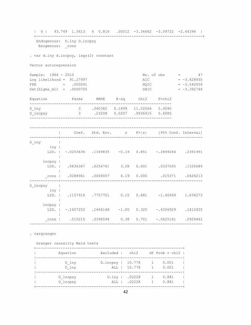
9.2.2 Growth versus domestic credit to the private sector
The null hypothesis that domestic credit to private sector does not Granger causes real GDP
growth is flatly rejected at the 1% level of statistical significance.
However, the null hypothesis that real GDP growth does not Granger causes financial
development, proxied by domestic credit to private sector is not rejected.
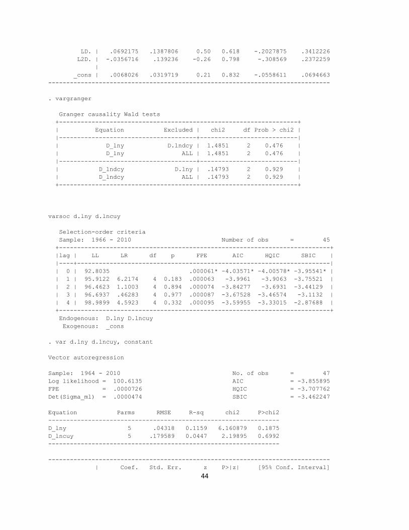
9.2.3 Growth versus total domestic credit
The null hypothesis that total domestic credit does not Granger causes real GDP growth and the
null hypothesis that real GDP growth does not Granger causes growth in total domestic credit as
percent of GDP cannot be rejected at all conventional levels of statistical significance.
9.2.4 Growth versus currency to GDP ratio
Similar to the case where financial development was proxied by total domestic credit, both null
hypothesis of non-causality are not rejected
25
9.3 Investigating the main determinants of growth
I determine the optimal lag differences to include in the vector error-correction and the number
of cointegration ranks. Estimation of the long and short run elasticities via the use of the VECM
is done. The optimal lag selected based on the AIC is 2.
Having determined the optimal lag length of 2 for the VAR based on the AIC, I proceed to test
the existence of cointegration and hence a stable long run equilibrium relationship among the
concerned variables. This is done by the use of Johansen (1988, 1995) multivariate cointegration
technique.
The null hypothesis that the number of cointegration rank is zero is implying no cointegration
among the variables is flatly rejected by the Trace statistic. . However the null hypothesis that
the cointegration rank is equal to 1 cannot be rejected. Therefore I concluded that there is
cointegration between real GDP and its determinants and that the number of cointegrating
equations is unit. The implication of this is that, there is common stochastic trend among the
variables in the selected model.
9.4 The long run relationship between growth and its determinants
From the results of the cointegrating relationship between growth and its determinants, it is
found that all the explanatory variables, with the exception of inflation rate, are statistically
significant at 1% level.
26
9.5 The short run relationship (vector error-correction model)
The short run results show that the error connection term is appropriately signed (negative) and
statistically significant at 1% level ensuring the attainment of long run equilibrium following a
shock. The coefficient of error correction term measures the speed of adjustment of real GDP
growth to long run equilibrium due to changes in the capital stock, labour force, trade openness,
inflation and ratio of domestic credit to private sector to GDP.The coefficient of error correction
term is -0.2366, indicating that only 23.66% of a deviation from the long run in the previous is
corrected in the current year.
10 Analysis
There is evidence of unit root in the variables which means that the variables do not revert to
their means following a shock. In order words, a shock to any of the integrated variables will
have permanent effects on all future time path of the variable.
In testing for causality between economic growth and four proxies of financial development,
growth versus broad money supply indicated that past growth rate in broad money supply does
not help in predicting current and future growth rate of real GDP in Ghana since the lags terms of
money supply in the growth equation are not statistically significant.However,the lags of GDP
growth included in money supply equation are significant; indicating that the past growth rate of
the economy has important predictive power on the current and future growth rates of broad
money supply. This suggests that it is economic growth that leads to financial development,
when financial development is proxied by growth in broad money supply as ratio to GDP, and
27
not the other way round as purported in the finance growth literature. Thus, when financial
development is measured by growth in broad money supply, there will not be any meaningful
causal effect from broad money growth to real GDP; hence I cannot use this variable as a
covariate in a standard growth equation to be presented later in this chapter due to the reverse
causality from growth to broad money supply.
The non rejection of the null hypothesis that real GDP growth does not Granger causes financial
development, proxied by domestic credit to private sector are in sharp contrast to those obtained
when financial development was proxied by broad money supply to GDP ratio. There exist a one
way causality running from financial development proxied by domestic credit to private sector to
real GDP growth.
Interestingly, both the null hypothesis that total domestic credit does not Granger causes real
GDP growth and the null hypothesis that GDP does not Granger causes growth in total domestic
credit as percent of GDP cannot be rejected at all conventional levels of statistical significance.
Furthermore, there is no Granger causal relationship between economic growth and financial
development, when financial development is measured as total currency to GDP ratio.
On the whole, the results emanating from the Granger causality analysis are quite interesting.
The existence and direction of causality depends on what proxy is used for financial
development. When financial development is proxied by either total domestic credit or total
currency as a ratio to GDP, no evidence of causality exists at all, between economic growth and
financial development.

28
These conflicting findings here support the debate in the literature as to whether there is any
causal link at all between finance and growth and whether it is growth that causes financial
development or it is financial development that causes growth.
Another interesting point worth emphasizing from the causality analysis is the fact that it is
credit to private sector that matters for growth and not the total credit. This point to the fact that
capital allocation between private and public sector use has great potential growth effect. This
also supports the crowding-out argument usually used against growing public sector activity.
The results from the cointegration test imply that these variables, namely, capital stock, labour
force, trade openness, and domestic credit to private sector are important determinants of
economic growth in the long-run. Contrary to theoretical expectations, the coefficients of capital
stock, labour force, and domestic credit to the private sector are found to be wrongly signed. In
contrast, the signs on the coefficients of trade openness and inflation rate are consistent with
priori expectations.
The results indicate that the output elasticity of capital stock is -0.2789, implying that, all other
things being equal, a 1% expansion in the economy’s capital stock in a given year will depress
the economy’s output level by 0.279%. Intuitively, this result suggests that growth in capital
stock significantly exerts a negative impact on output and therefore economic growth in the long
run.
Whilst this finding defies the predictions of the neoclassical growth theory, it can be argued that
given the existing production system (and technology) capital is too large and is

29
disproportionately combined with other inputs such that the marginal productivity of capital
diminishes with addition to the economy’s capital.
Once again, it is surprising and intriguing to find that the estimated long run relationship between
GDP and labour is negative and statistically significant. Tentatively, it is expected that additions
to the labour force will increase output in the long run and not reduce it. However, the results
flout this expectation. The cointegration results also show that a 1% growth in the economy’s
labour force (due to population growth) significantly reduces real output by almost 1% (0.9964).
This finding is consistent with the Solow growth model, which posits that an increase in the rate
of population growth is detrimental to economic growth in the long run. Empirically, this
outcome is consistent with the findings of Baafi Antwi (2010), Sakyi (2011) and Aryeetey and
Fosu (2002), who in various ways examined the determinants of economic growth in Ghana.
According to Baafi Antwi (2010) this outcome can be attributed to fact that “…labour is
proportionately too large than capital such that the marginal productivity of labour is negative…”
Baafi further noted that, taking into account the unskilled labour force (in terms of nutrition,
health and education), mass unemployment and underemployment, that are widespread in the
country implies that large proportion of the workforce are not working. In addition to these
factors, Sakyi (2011) argued that the frequent industrial actions and the way the labour market is
regulated, coupled with labour intensive agriculture and petty trading with limited employment
benefits that characterized the labour market in Ghana and other developing economies, and the
possibility of diminishing marginal returns to capital may explain the adverse growth effects of
labour force in Ghana. Thus, additional labour does not add anything to output-They rather
reduce it.

30
From the results, a 1% increase in the degree of the economy’s openness to the foreign trade
promotes growth in real GDP in the long run by 0.392%, all other things being equal. This
provides yet another evidence for the classical view that free trade would cause world resources
to be utilized most efficiently, promote economic growth and maximize world welfare
(Salvatore, 1996). Indeed, openness to trade provides access to imported inputs embodying new
technology, increases the size of the market faced by the domestic producers raising the returns
to innovation, and facilitates a country’s specialization in research-intensive production. This
finding is in harmony with Sakyi (2011), Matadeen, and Seetanah (2011), Azam and Khattak
(2009), Sakar (2007) and Yanikkaya (2003) among others.
This study show that inflationary situation (an indicator of macroeconomic instability and
uncertainty) is found to propel real GDP growth in the long run. However, the results show that
inflation rate has no significant explanatory power as far as growth in real GDP is concern as its
coefficient is very negligible (0.000178) and it is not statistically different from zero at 5%
significance level. Theoretically, a high inflation rate is expected to be deleterious to growth in
real GDP as it raises the cost of borrowing which in turn dampens the rate of investment by the
private sector and thus decreases real output growth. Whilst the result obtained in this study
indicates the reverse, it can be argued that, it is consistent with the structuralist view that
inflation is essential for economic growth and therefore has a positive effect on growth. This
view is based on the contention that inflation is a mechanism which induces forced savings.
When the government of a developing country finds that its fiscal system is inadequate, it may
begin borrowing from the central bank to finance spending and this creates inflationary finance
that increases capital movements necessary for economic growth (Jung & Marshall, 1986). As
Khan and Senhadji (2001) have argued, there is a threshold beyond which inflation is harmful to

31
growth; as such creeping inflation in itself is not detrimental to growth. Antwi, Mills and Zhao
(2010) obtained similar results for Ghana and Hussein and Malik (2011), Chowdhury (2001)
found similar results in Bangladesh, India, Pakistan and Sri Lanka in comparative studies.
Contradictorily, Shahbaz, Ahmad, and Chaudhary (2009) and Prasanna and Gopakumar (n.d.)
found inflation to be rather harmful to growth in the long run in Pakistan and India respectively.
From the results, the estimated elasticity of real GDP with respect to domestic credit to the
private sector is -0.361, indicating that, ceteris paribus, a 1% increase in the domestic credit
available to the private sector reduces real output by 0.361%. Domestic credit to the private
sector indicator of financial development conflicts with Mackinnon-Shaw’s finance-led growth
hypothesis and the findings of many empirical studies that provide credence to this hypothesis.
Goaied and Sassi (2010) suggested that this negative relationship between financial development
and economic growth can be attributed to the underdeveloped financial systems and the high
degree of financial repression in many economies, particularly in developing countries. These,
among other factors, restrain the activity of the financial intermediaries to increase the
mobilization of savings; supply funds and feed economic growth through the channel of
increased investment.
All the explanatory variables preserved their respective signs and statistical status, although
changes in capital stock and labour force turned out to be insignificant in the short run.
11 Conclusion
This study analyses the relationship between financial development and economic growth.
Modern time series econometric techniques were used to examine this nexus. It was found out

32
that the existence and direction of causality depends on what proxy is used for financial
development and it was discovered that finance follows in the direction of economic growth but
does not necessarily lead to it and that capital allocation between private and public sector use
has great potential growth effect.
From the Cointegration results these variables, namely, capital stock, labour force, trade
openness and domestic credit to private sector are important determinants of economic growth
in the long-run but do not establish a long run relationship between financial development and
economic growth.
Another unconventional result obtained in this study is that inflation situation (an indicator of
macroeconomic instability and uncertainty) is found to propel real GDP growth in the long run.
Comparatively, changes in capital stock and inflation are found to have higher impact on real
GDP growth in the short run than in the long run. On the other hand, the elasticities of real GDP
with respect to labour force, trade openness and domestic credit to private sector are lower in the
short run than in long run. Thus the positive impact of changes in trade openness and the
negative effect of domestic credit to private sector on economic growth are more profound in the
long run than in the short run.
This suggests the possibility of sluggish adjustment from disequilibrium to the steady state level.
33
12 References
Abu Nurudeen, Does Stock Market Development Raise Economic Growth?,
2009.
Allen, F. and D. Gale (2000), “Comparing Financial Systems, Cambridge, MA: MIT Press
Allen, F., J. Qian, and M. Qian (2005), “Law, Finance, and Economic Growth in China”, Journal
of Financial Economics, forthcoming
Arestis, P., P. O. Demetriades and K. B. Luintel (2001), “Financial Development and Economic
Growth: The Role of Stock Markets”, Journal of Money, Credit, and Banking, 33: 16-41.
Arestis, P. and P. Demetriades (1997), “Financial Development and Economic Growth:
Assessing the Evidence”, Economic Journal, 107: 783-799.
Atje, R. and B. Jovanovic (1993), "Stock Markets and Development”, European Economic
Review, 37: 632-640.
Beck T., Levine R., Loayza N. (2000), “Finance and the Sources of Growth”, Journal of
Financial Economics, 58(1-2), 261-300.
Beck T. (2008), “The Econometrics of Finance and Growth”, Policy Research Working
Paper Series 4608, the World Bank.
Berger, A.N., I. Hasan, and L.F. Klapper (2004), “Further Evidence on the Link between Finance
and Growth: An International Analysis of Community Banking and Economic
Performance”, Journal of Financial Services Research, forthcoming.
Carlin, W. and C. Mayer (2003), “Finance, Investment, and Growth”, Journal of Financial
Economics, 69: 191-226
Christopoulosa DK, Tsionas EG (2004). Financial development and economic growth: evidence
from panel unit root and cointegration tests. J. Dev. Econ., 73: 55-74.
Christopoulos, D. K. and E. G. Tsionas (2004), “Financial Development and Economic Growth:
Evidence from Panel Unit Root and Cointegration Tests”, Journal of Development Economics,
73: 55-74.
Darrat, A., 1999. Are financial deepening and economic growth causally related? Another look
at the evidence. International Economic Journal 13, 19–35.

34
Demetriades PO, Hussein AK (1996). Does financial development cause economic growth?
Time series evidence from 16 countries. Dev. Econ., 51: 387-411.
Demirgüç-Kunt, A. and R. Levine (2001c), Financial Structures and Economic Growth: A Cross-
Country Comparison of Banks, Markets, and Development, Cambridge, MA: MIT Press.
F. N’zue, Stock Market Development and Economic Growth: Evidence from CoteD’Ivore,
Africa Development Review, 18(1), (2006), 123-145.
Granger C.W.J., Lin J. L. (1995),“Causality in the long run”, Econometric Theory, 11 (3),
530-36.
Hagmayr B., Haiss P.R., Sumegi K. (2007), “Financial Sector Development and Economic
Growth - Evidence for Southeastern Europe” EuropaInstitut Working Paper.
Harrison P., Sussman O., Zeira J. (1999), “Finance and growth: Theory and new evidence”,
Finance and Economics Discussion Series 35, The Federal Reserve Board
Im K., Pesaran M.H., Shin Y. (2003), “Testing for unit roots in heterogeneous panels”,
Journal of Econometrics 115 (1), 53-74.
Im, S.K., Pesaran, H.M., Shin, Y., 1997. Testing for Unit Roots in Heterogeneous Panel.
Department of Applied Econometrics, University of Cambridge.
Jung, W. S. (1986), "Financial Development and Economic Growth: International Evidence”,
Economic Development and Cultural Change, 34: 333-346.
Khan, S.M., Senhadji, A.S., 2000. Financial Development and Economic Growth: An Overview.
IMF Working Paper. International Monetary Fund, Washington.
King R.G., Levine R (1993b), “Finance and Growth: Schumpeter might be right”, Quarterly
Journal of Economics, 108 (3), 717-37.
King, R. G and Ross Levine (1993a) Finance, Entrepreneurship, and Growth, Journal of
Monetary Economics, 32, 513-42.
King, R. G. and R. Levine (1993b), "Finance, Entrepreneurship, and Growth: Theory and
Evidence”, Journal of Monetary Economics, 32: 513-542.
King, R. G. and R. Levine (1993c), "Financial Intermediation and Economic Development”,
Financial Intermediation in the Construction of Europe, Eds: C. Mayer and X. Vives,
Kenourgios D., Samitas A. (2007).” Financial Development and Economic Growth in a
Transition Economy: Evidence for Poland” Journal of Financial Decision Making, 3, (1), 35-
48.

35
Kerry Patterson, An Introduction to Applied Econometrics: A Time Series
Approach, 2000
Levine R., Loayza N., Beck T. (2000), “Financial intermediation and growth: Causality and
Causes”, Journal of Monetary Economics, 46(1), 31-77.
Levine, R., N. Loayza and T. Beck (2000), “Financial Intermediation and Growth: Causality and
Causes”, Journal of Monetary Economics, 46: 31-77.
Levine R., Zervos S. (1996), “Stock Market Development and Long-Run Growth”, World
Bank Economic Review, 10(2), 323-339.
Levine R. (2005), “Finance and Growth: Theory and Evidence,” Handbook of Economic
Growth, in: Aghion P. and S. Durlauf (ed.), vol 1, 865-934.
Levine, R. (1999). "Law, Finance, and Economic Growth”. Journal of Financial
Intermediation. 8, 8-35.
Luintel, K.B. and Khan, M. (1999) A Quantitative Reassessment of the Finance-Growth Nexus:
Evidence from a Multivariate VAR, Journal of Development Economics, 60, 381-405.
London: Centre for Economic Policy Research: 156-189.
Miller, M. H. (1998), "Financial Markets and Economic Growth", Journal of Applied Corporate
Finance, 11: 8-14.
Odhiambo, N.M. (2004). "Is Financial Development still a Spur to Economic Growth?
Patrick HT (1966). Financial development and economic growth in underdeveloped
countries.Econ. Dev. Cultural Change, 14: 174-189.
Patrick, H. (1966). "Financial Development and Economic Growth in Underdeveloped
Countries”. Economic Development and Cultural Change, 174-189.
Rajan, R. G. and L. Zingales (1998), “Financial Dependence and Growth”, American Economic
Review, 88: 559-586.
Robinson, J. (1952). The Rate of Interest and Other Essays. Macmillan, London.
Schumpeter JA (1911). The theory of economic development. (Harvard
University Press, Cambridge, MA).

36
Schumpeter, J.A. (1911). The Theory of Economic Development: An Inquiry into Profits,
Capital, Credit, Interest and the Business Cycle. Translated and Reprinted 1961, New York:
Oxford University Press.
Shan, Jordan Z; Morris, Alan G; Sun, Fiona.(2001). Financial Development and Economic
Growth: An Egg-and-Chicken Problem? , Review of International Economics, 9 (3): 443-454.
Shahnoushi. N, et. Al. (2008). "Causality between Financial Development and Economic Growth
in Iran". World Applied Science Journal. 4(5):736-740.
Shan, J. Z., A. G. Morris and F. Sun (2001), “Financial Development and Economic Growth: An
Egg and Chicken Problem?” Review of International Economics, 9: 443-454.
Stulz, R. M. (2001), “Does Financial Structure Matter for Economic Growth? A Corporate
Finance Perspective”, In: Financial Structure and Economic Growth: A Cross-Country
Comparison of Banks, Markets, and Development, Eds: A. Demirguc-Kunt and R.
Levine. Cambridge, MA: MIT Press: 143-188.
Sussman, O. (1993), “A Theory of Financial Development”, In: Finance and Development:
Issues and Experience, Ed: A. Giovannini, (Cambridge: Cambridge University Press):
29-64.
Temple, J. (1999), “The New Growth Evidence”, Journal of Economic Literature, 37: 112-156.
Wachtel P. (2001), “Growth and Finance: What do we know and how do we know it?”,
International Finance, 4(3), 335-362
13 APPENDIX
Results of the unit root test
Table 1: Results of Unit Root Test
Variables ADF Test Results PP Test Results
Constant Constant &
Trend
Constant Constant &
Trend
LEVEL (LOG LEVELS)
lnY 2.008 -0.387 2.150 -0.196
lnK -1.245 -2.301 -1.506 -2.311
lnL -0.080 -0.844 -0.236 -1.678
lnTrade -1.305 -1.926 -1.485 -2.088
Infl -2.256 -2.242 -4.402*** -4.343***
lnM2+/Y -1.599 -1.821 -1.896 -2.118

37
lncpsy -0.672 -1.105 -0.928 -1.233
lndcy -3.341** -3.254* -3.539** 3.332*
lncuy -2.383 -2.489 -2.865 -3.042
FIRST DIFFERENCES
lnY -3.016** -3.895** -4.767*** -5.301***
lnK -4.470*** -4.654*** -6.864*** -6.933***
lnL -4.698*** -4.639*** -2.789* -2.766
lnTrade -3.439*** -3.392** -4.695*** -4.638***
Infl -5.555*** -5.567*** -13.887*** -13.949***
lnM2+/Y -3.977*** -3.998** -7.005*** -6.955***
lncpsy -3.165** -3.317** -6.474*** -6.527***
lndcy -4.299*** -4.107** -6.369*** -8.095***
lncuy -4.029*** -3.982** -8.185*** -8.095***
proxy of financial development(GRANGER CAUSALITY TEST)
GDP to growth of broad money supply
Table 2: Granger causality Wald tests
+------------------------------------------------------------------+
| Equation Excluded | chi2 df Prob > chi2 |
|--------------------------------------+---------------------------|
| D_lny D.lnm2_y | .00098 1 0.975 |
| D_lny ALL | .00098 1 0.975 |
|--------------------------------------+---------------------------|
| D_lnm2_y D.lny | 4.13 1 0.042 |
| D_lnm2_y ALL | 4.13 1 0.042 |
GDP to domestic credit to the private sector
Table 3: Granger causality Wald tests +------------------------------------------------------------------+ | Equation Excluded | chi2 df Prob > chi2 |
|--------------------------------------+---------------------------|
| D_lny D.lncpsy | 10.778 1 0.001 |
| D_lny ALL | 10.778 1 0.001 |
|--------------------------------------+---------------------------|
| D_lncpsy D.lny | .02228 1 0.881 |
| D_lncpsy ALL | .02228 1 0.881 |
+------------------------------------------------------------------+
Table 4: Granger causality Wald tests +------------------------------------------------------------------+

38
| Equation Excluded | chi2 df Prob > chi2 |
|--------------------------------------+---------------------------|
| D_lny D.lndcy | 1.4851 2 0.476 |
| D_lny ALL | 1.4851 2 0.476 |
|--------------------------------------+---------------------------|
| D_lndcy D.lny | .14793 2 0.929 |
| D_lndcy ALL | .14793 2 0.929 |
+------------------------------------------------------------------+
GDP the total currency as a ratio to GDP (monetization ratio
Table 5: Granger causality Wald tests +------------------------------------------------------------------+
| Equation Excluded | chi2 df Prob > chi2 |
|--------------------------------------+---------------------------|
| D_lny D.lncuy | .48796 2 0.784 |
| D_lny ALL | .48796 2 0.784 |
|--------------------------------------+---------------------------|
| D_lncuy D.lny | .19026 2 0.909 |
| D_lncuy ALL | .19026 2 0.909 |
+------------------------------------------------------------------+
Table 6: Determination of Cointegration Rank
Johansen tests for cointegration
Trend: constant Number of obs = 48
Sample: 1963 - 2010 Lags = 2
-------------------------------------------------------------------------------
5%
Maximum trace critical
Rank parms LL eigenvalue statistic value
0 42 154.27233 . 111.1992 94.15
1 53 177.64184 0.62233 64.4602* 68.52
2 62 192.67818 0.46555 34.3875 47.21
3 69 203.98595 0.37572 11.7720 29.68
4 74 208.02214 0.15479 3.6996 15.41
5 77 209.77259 0.07034 0.1987 3.76
6 78 209.87194 0.00413
-------------------------------------------------------------------------------

39
Table 7: Cointegrating equations
Equation Parms chi2 P>chi2
-------------------------------------------
_ce1 5 1750.707 0.0000
-------------------------------------------
Identification: beta is exactly identified
Johansen normalization restriction imposed
------------------------------------------------------------------------------
beta | Coef. Std. Err. z P>|z| [95% Conf. Interval]
-------------+----------------------------------------------------------------
_ce1 |
lny | 1 . . . . .
lnk | -.2789611 .0623688 -4.47 0.000 -.4012017 -.1567205
lnl | -.9964418 .0370503 -26.89 0.000 -1.069059 -.9238246
lntrade | .392343 .0660534 5.94 0.000 .2628808 .5218053
infl | .0001786 .0007026 0.25 0.799 -.0011984 .0015556
lncpsy | -.3610883 .0347534 -10.39 0.000 -.4292038 -.2929729
_cons | -7.543107 . . . . .
------------------------------------------------------------------------------
9.5 The short run relationship (vector error-correction model)
Sample: 1963 - 2010 No. of obs = 48
AIC = -5.19341
Log likelihood = 177.6418 HQIC = -4.412621
Det(Sigma_ml) = 2.46e-11 SBIC = -3.127292
Equation Parms RMSE R-sq chi2 P>chi2
----------------------------------------------------------------
D_lny 8 .036134 0.6060 61.51541 0.0000
D_lnk 8 .179251 0.5268 44.53697 0.0000
D_lnl 8 .001941 0.9953 8437.037 0.0000
D_lntrade 8 .169705 0.5112 41.83632 0.0000
D_infl 8 26.3366 0.3603 22.53406 0.0040
D_lncpsy 8 .221438 0.2069 10.43335 0.2359
----------------------------------------------------------------
------------------------------------------------------------------------------
| Coef. Std. Err. z P>|z| [95% Conf. Interval]
-------------+----------------------------------------------------------------
D_lny |
_ce1 |
L1. | -.2366001 .0727527 -3.25 0.001 -.3791927 -.0940076
|
lny |

40
LD. | .4287189 .1362157 3.15 0.002 .161741 .6956967
|
lnk |
LD. | -.039353 .0277075 -1.42 0.156 -.0936588 .0149528
|
lnl |
LD. | -.544565 1.36949 -0.40 0.691 -3.228716 2.139586
|
lntrade |
LD. | .1059543 .0302732 3.50 0.000 .04662 .1652886
|
infl |
LD. | .0002535 .0001818 1.39 0.163 -.0001029 .0006099
|
lncpsy |
LD. | -.0711956 .032654 -2.18 0.029 -.1351962 -.007195
|
_cons | .2181337 .0668301 3.26 0.001 .0871492 .3491182
-------------+----------------------------------------------------------------
GRANGER CAUSALITY TEST BASED ON STATIONARY VAR MODEL varsoc d.lny d.lnm2_y
Selection-order criteria
Sample: 1966 - 2010 Number of obs = 45
+---------------------------------------------------------------------------+
|lag | LL LR df p FPE AIC HQIC SBIC |
|----+----------------------------------------------------------------------|
| 0 | 106.142 .000033 -4.62853 -4.5986* -4.54824* |
| 1 | 111.054 9.8241* 4 0.043 .000032* -4.66907* -4.57927 -4.42818 |
| 2 | 112.299 2.4907 4 0.646 .000036 -4.54664 -4.39697 -4.14516 |
| 3 | 112.476 .35246 4 0.986 .000043 -4.3767 -4.16716 -3.81462 |
| 4 | 114.376 3.8001 4 0.434 .000048 -4.28337 -4.01396 -3.5607 |
+---------------------------------------------------------------------------+
Endogenous: D.lny D.lnm2_y
Exogenous: _cons
. var d.lny d.lnm2_y, lags(1) constant
Vector autoregression
Sample: 1963 - 2010 No. of obs = 48
Log likelihood = 119.255 AIC = -4.718958
FPE = .0000306 HQIC = -4.630566
Det(Sigma_ml) = .0000238 SBIC = -4.485057
Equation Parms RMSE R-sq chi2 P>chi2
----------------------------------------------------------------
D_lny 3 .041996 0.1057 5.67211 0.0587

41
D_lnm2_y 3 .125382 0.0800 4.17324 0.1241
----------------------------------------------------------------
------------------------------------------------------------------------------
| Coef. Std. Err. z P>|z| [95% Conf. Interval]
-------------+----------------------------------------------------------------
D_lny |
lny |
LD. | .3272228 .1374791 2.38 0.017 .0577687 .5966769
|
lnm2_y |
LD. | .0014543 .0463543 0.03 0.975 -.0893985 .0923071
|
_cons | .0204744 .0071719 2.85 0.004 .0064177 .0345311
-------------+----------------------------------------------------------------
D_lnm2_y |
lny |
LD. | .8341405 .4104519 2.03 0.042 .0296694 1.638612
|
lnm2_y |
LD. | -.0152001 .1383935 -0.11 0.913 -.2864465 .2560463
|
_cons | -.0166679 .0214121 -0.78 0.436 -.0586349 .0252991
------------------------------------------------------------------------------
vargranger
Granger causality Wald tests
+------------------------------------------------------------------+
| Equation Excluded | chi2 df Prob > chi2 |
|--------------------------------------+---------------------------|
| D_lny D.lnm2_y | .00098 1 0.975 |
| D_lny ALL | .00098 1 0.975 |
|--------------------------------------+---------------------------|
| D_lnm2_y D.lny | 4.13 1 0.042 |
| D_lnm2_y ALL | 4.13 1 0.042 |
+------------------------------------------------------------------+
varsoc d.lny d.lncpsy
Selection-order criteria
Sample: 1966 - 2010 Number of obs = 45
+---------------------------------------------------------------------------+
|lag | LL LR df p FPE AIC HQIC SBIC |
|----+----------------------------------------------------------------------|
| 0 | 79.7121 .000108 -3.45387 -3.42394 -3.37358* |
| 1 | 83.4252 7.4261 4 0.115 .00011 -3.44112 -3.35132 -3.20023 |
| 2 | 90.9603 15.07* 4 0.005 .000094* -3.59823* -3.44857* -3.19675 |
| 3 | 92.9684 4.0162 4 0.404 .000103 -3.50971 -3.30017 -2.94763 |
42
| 4 | 93.749 1.5613 4 0.816 .00012 -3.36662 -3.09722 -2.64396 |
+---------------------------------------------------------------------------+
Endogenous: D.lny D.lncpsy
Exogenous: _cons
. var d.lny d.lncpsy, lags(2) constant
Vector autoregression
Sample: 1964 - 2010 No. of obs = 47
Log likelihood = 91.27997 AIC = -3.628935
FPE = .000091 HQIC = -3.540056
Det(Sigma_ml) = .0000705 SBIC = -3.392746
Equation Parms RMSE R-sq chi2 P>chi2
----------------------------------------------------------------
D_lny 3 .040382 0.1899 11.02064 0.0040
D_lncpsy 3 .23208 0.0207 .9936415 0.6085
----------------------------------------------------------------
------------------------------------------------------------------------------
| Coef. Std. Err. z P>|z| [95% Conf. Interval]
-------------+----------------------------------------------------------------
D_lny |
lny |
L2D. | -.0253636 .1349835 -0.19 0.851 -.2899264 .2391991
|
lncpsy |
L2D. | .0836367 .0254761 3.28 0.001 .0337045 .1335689
|
_cons | .0288961 .0069007 4.19 0.000 .015371 .0424213
-------------+----------------------------------------------------------------
D_lncpsy |
lny |
L2D. | .1157916 .7757701 0.15 0.881 -1.40469 1.636273
|
lncpsy |
L2D. | -.1457252 .1464148 -1.00 0.320 -.4326929 .1412425
|
_cons | .015215 .0396594 0.38 0.701 -.0625161 .0929461
------------------------------------------------------------------------------
. vargranger
Granger causality Wald tests
+------------------------------------------------------------------+
| Equation Excluded | chi2 df Prob > chi2 |
|--------------------------------------+---------------------------|
| D_lny D.lncpsy | 10.778 1 0.001 |
| D_lny ALL | 10.778 1 0.001 |
|--------------------------------------+---------------------------|
| D_lncpsy D.lny | .02228 1 0.881 |
| D_lncpsy ALL | .02228 1 0.881 |
+------------------------------------------------------------------+

43
varsoc d.lny d.lndcy
Selection-order criteria
Sample: 1966 - 2010 Number of obs = 45
+---------------------------------------------------------------------------+
|lag | LL LR df p FPE AIC HQIC SBIC |
|----+----------------------------------------------------------------------|
| 0 | 95.4064 .000054* -4.1514* -4.12146* -4.0711* |
| 1 | 98.2663 5.7197 4 0.221 .000057 -4.10072 -4.01092 -3.85984 |
| 2 | 98.7611 .98961 4 0.911 .000066 -3.94494 -3.79527 -3.54346 |
| 3 | 99.1104 .69852 4 0.952 .000078 -3.78268 -3.57315 -3.22061 |
| 4 | 99.5724 .92404 4 0.921 .000092 -3.62544 -3.35604 -2.90277 |
+---------------------------------------------------------------------------+
Endogenous: D.lny D.lndcy
Exogenous: _cons
. var d.lny d.lndcy, constant
Vector autoregression
Sample: 1964 - 2010 No. of obs = 47
Log likelihood = 102.3205 AIC = -3.92853
FPE = .0000675 HQIC = -3.780398
Det(Sigma_ml) = .0000441 SBIC = -3.534882
Equation Parms RMSE R-sq chi2 P>chi2
----------------------------------------------------------------
D_lny 5 .042734 0.1341 7.27717 0.1219
D_lndcy 5 .174476 0.0097 .4581773 0.9774
----------------------------------------------------------------
------------------------------------------------------------------------------
| Coef. Std. Err. z P>|z| [95% Conf. Interval]
-------------+----------------------------------------------------------------
D_lny |
Lny |
LD. | .3460153 .1456025 2.38 0.017 .0606396 .631391
L2D. | -.0314096 .1448769 -0.22 0.828 -.315363 .2525438
|
lndcy |
LD. | -.0290961 .0339909 -0.86 0.392 -.095717 .0375249
L2D. | .0312036 .0341024 0.91 0.360 -.0356359 .0980432
|
_cons | .0206112 .0078307 2.63 0.008 .0052632 .0359591
-------------+----------------------------------------------------------------
D_lndcy |
lny |
LD. | .2178261 .5944768 0.37 0.714 -.947327 1.382979
L2D. | -.004292 .5915141 -0.01 0.994 -1.163638 1.155054
|
lndcy |
44
LD. | .0692175 .1387806 0.50 0.618 -.2027875 .3412226
L2D. | -.0356716 .139236 -0.26 0.798 -.308569 .2372259
|
_cons | .0068026 .0319719 0.21 0.832 -.0558611 .0694663
------------------------------------------------------------------------------
. vargranger
Granger causality Wald tests
+------------------------------------------------------------------+
| Equation Excluded | chi2 df Prob > chi2 |
|--------------------------------------+---------------------------|
| D_lny D.lndcy | 1.4851 2 0.476 |
| D_lny ALL | 1.4851 2 0.476 |
|--------------------------------------+---------------------------|
| D_lndcy D.lny | .14793 2 0.929 |
| D_lndcy ALL | .14793 2 0.929 |
+------------------------------------------------------------------+
varsoc d.lny d.lncuy
Selection-order criteria
Sample: 1966 - 2010 Number of obs = 45
+---------------------------------------------------------------------------+
|lag | LL LR df p FPE AIC HQIC SBIC |
|----+----------------------------------------------------------------------|
| 0 | 92.8035 .000061* -4.03571* -4.00578* -3.95541* |
| 1 | 95.9122 6.2174 4 0.183 .000063 -3.9961 -3.9063 -3.75521 |
| 2 | 96.4623 1.1003 4 0.894 .000074 -3.84277 -3.6931 -3.44129 |
| 3 | 96.6937 .46283 4 0.977 .000087 -3.67528 -3.46574 -3.1132 |
| 4 | 98.9899 4.5923 4 0.332 .000095 -3.59955 -3.33015 -2.87688 |
+---------------------------------------------------------------------------+
Endogenous: D.lny D.lncuy
Exogenous: _cons
. var d.lny d.lncuy, constant
Vector autoregression
Sample: 1964 - 2010 No. of obs = 47
Log likelihood = 100.6135 AIC = -3.855895
FPE = .0000726 HQIC = -3.707762
Det(Sigma_ml) = .0000474 SBIC = -3.462247
Equation Parms RMSE R-sq chi2 P>chi2
----------------------------------------------------------------
D_lny 5 .04318 0.1159 6.160879 0.1875
D_lncuy 5 .179589 0.0447 2.19895 0.6992
----------------------------------------------------------------
------------------------------------------------------------------------------
| Coef. Std. Err. z P>|z| [95% Conf. Interval]

45
-------------+----------------------------------------------------------------
D_lny |
lny |
LD. | .341448 .1472786 2.32 0.020 .0527871 .6301088
L2D. | -.0340819 .1466948 -0.23 0.816 -.3215984 .2534346
|
lncuy |
LD. | -.0060703 .0353182 -0.17 0.864 -.0752927 .0631522
L2D. | .0222779 .0352185 0.63 0.527 -.046749 .0913048
|
_cons | .0210488 .0077772 2.71 0.007 .0058058 .0362919
-------------+----------------------------------------------------------------
D_lncuy |
lny |
LD. | .0365329 .6125462 0.06 0.952 -1.164036 1.237101
L2D. | .2378781 .6101179 0.39 0.697 -.957931 1.433687
|
lncuy |
LD. | -.1965375 .1468919 -1.34 0.181 -.4844404 .0913653
L2D. | -.0920407 .146477 -0.63 0.530 -.3791304 .195049
|
_cons | -.0185637 .0323462 -0.57 0.566 -.081961 .0448337
------------------------------------------------------------------------------
. vargranger
Granger causality Wald tests
+------------------------------------------------------------------+
| Equation Excluded | chi2 df Prob > chi2 |
|--------------------------------------+---------------------------|
| D_lny D.lncuy | .48796 2 0.784 |
| D_lny ALL | .48796 2 0.784 |
|--------------------------------------+---------------------------|
| D_lncuy D.lny | .19026 2 0.909 |
| D_lncuy ALL | .19026 2 0.909 |
+------------------------------------------------------------------+
Cointegration Rank Determination vecrank lny lnk lnl lntrade infl lncpsy, lags(2)
Johansen tests for cointegration
Trend: constant Number of obs = 48
Sample: 1963 - 2010 Lags = 2
-------------------------------------------------------------------------------
5%
Maximum trace critical

46
Rank parms LL eigenvalue statistic value
0 42 154.27233 . 111.1992 94.15
1 53 177.64184 0.62233 64.4602* 68.52
2 62 192.67818 0.46555 34.3875 47.21
3 69 203.98595 0.37572 11.7720 29.68
4 74 208.02214 0.15479 3.6996 15.41
5 77 209.77259 0.07034 0.1987 3.76
6 78 209.87194 0.00413
-------------------------------------------------------------------------------
VECM Estimates vec lny lnk lnl lntrade infl lncpsy, rank(1)
Vector error-correction model
Sample: 1963 - 2010 No. of obs = 48
AIC = -5.19341
Log likelihood = 177,6418 HQIC = -4.412621
Det(Sigma_ml) = 2.46e-11 SBIC = -3.127292
Equation Parms RMSE R-sq chi2 P>chi2
----------------------------------------------------------------
D_lny 8 .036134 0.6060 61.51541 0.0000
D_lnk 8 .179251 0.5268 44.53697 0.0000
D_lnl 8 .001941 0.9953 8437.037 0.0000
D_lntrade 8 .169705 0.5112 41.83632 0.0000
D_infl 8 26.3366 0.3603 22.53406 0.0040
D_lncpsy 8 .221438 0.2069 10.43335 0.2359
----------------------------------------------------------------
------------------------------------------------------------------------------
| Coef. Std. Err. z P>|z| [95% Conf. Interval]
-------------+----------------------------------------------------------------
D_lny |
_ce1 |
L1. | -.2366001 .0727527 -3.25 0.001 -.3791927 -.0940076
|
lny |
LD. | .4287189 .1362157 3.15 0.002 .161741 .6956967
|
lnk |
LD. | -.039353 .0277075 -1.42 0.156 -.0936588 .0149528
|
lnl |
LD. | -.544565 1.36949 -0.40 0.691 -3.228716 2.139586
|
lntrade |
LD. | .1059543 .0302732 3.50 0.000 .04662 .1652886
|
infl |
LD. | .0002535 .0001818 1.39 0.163 -.0001029 .0006099

47
|
lncpsy |
LD. | -.0711956 .032654 -2.18 0.029 -.1351962 -.007195
|
_cons | .2181337 .0668301 3.26 0.001 .0871492 .3491182
-------------+----------------------------------------------------------------
D_lnk |
_ce1 |
L1. | .8224319 .360901 2.28 0.023 .1150789 1.529785
|
lny |
LD. | .5803091 .6757194 0.86 0.390 -.7440766 1.904695
|
lnk |
LD. | -.4530449 .1374476 -3.30 0.001 -.7224373 -.1836526
|
lnl |
LD. | 15.05858 6.793572 2.22 0.027 1.74342 28.37373
|
lntrade |
LD. | .6179681 .1501748 4.11 0.000 .3236308 .9123053
|
infl |
LD. | -.0008595 .0009021 -0.95 0.341 -.0026275 .0009085
|
lncpsy |
LD. | .1518913 .1619851 0.94 0.348 -.1655937 .4693763
|
_cons | -1.050913 .3315211 -3.17 0.002 -1.700682 -.4011436
-------------+----------------------------------------------------------------
D_lnl |
_ce1 |
L1. | .0038138 .0039079 0.98 0.329 -.0038456 .0114732
|
lny |
LD. | .00312 .0073169 0.43 0.670 -.0112208 .0174608
|
lnk |
LD. | .0005572 .0014883 0.37 0.708 -.0023599 .0034742
|
lnl |
LD. | .9042791 .0735625 12.29 0.000 .7600993 1.048459
|
lntrade |
LD. | -.0024679 .0016261 -1.52 0.129 -.005655 .0007193
|
infl |
LD. | -4.94e-06 9.77e-06 -0.51 0.613 -.0000241 .0000142
|
lncpsy |
LD. | -.0005797 .001754 -0.33 0.741 -.0040175 .0028581
|
_cons | -.0007718 .0035898 -0.22 0.830 -.0078077 .0062641
-------------+----------------------------------------------------------------

48
D_lntrade |
_ce1 |
L1. | -1.035907 .3416816 -3.03 0.002 -1.705591 -.3662236
|
lny |
LD. | .5439914 .6397347 0.85 0.395 -.7098656 1.797848
|
lnk |
LD. | -.3532851 .130128 -2.71 0.007 -.6083312 -.0982389
|
lnl |
LD. | 20.13104 6.431787 3.13 0.002 7.524965 32.73711
|
lntrade |
LD. | .5436228 .1421774 3.82 0.000 .2649602 .8222854
|
infl |
LD. | -.0022042 .000854 -2.58 0.010 -.0038781 -.0005304
|
lncpsy |
LD. | -.2205466 .1533588 -1.44 0.150 -.5211243 .080031
|
_cons | .2876398 .3138663 0.92 0.359 -.3275268 .9028064
-------------+----------------------------------------------------------------
D_infl |
_ce1 |
L1. | 24.72792 53.02577 0.47 0.641 -79.20069 128.6565
|
lny |
LD. | -173.9972 99.28082 -1.75 0.080 -368.5841 20.58958
|
lnk |
LD. | -2.861274 20.19464 -0.14 0.887 -42.44204 36.71949
|
lnl |
LD. | -561.6556 998.153 -0.56 0.574 -2517.999 1394.688
|
lntrade |
LD. | -14.74043 22.0646 -0.67 0.504 -57.98625 28.50538
|
infl |
LD. | -.5560003 .1325372 -4.20 0.000 -.8157685 -.2962322
|
lncpsy |
LD. | 21.49108 23.79984 0.90 0.367 -25.15575 68.13791
|
_cons | .0651494 48.70909 0.00 0.999 -95.40292 95.53322
-------------+----------------------------------------------------------------
D_lncpsy |
_ce1 |
L1. | .5248248 .4458395 1.18 0.239 -.3490047 1.398654
|
lny |
LD. | 1.093047 .8347509 1.31 0.190 -.5430344 2.729129

49
|
lnk |
LD. | .1120416 .1697961 0.66 0.509 -.2207526 .4448359
|
lnl |
LD. | 12.91589 8.392448 1.54 0.124 -3.533001 29.36479
|
lntrade |
LD. | .0186176 .1855186 0.10 0.920 -.3449923 .3822274
|
infl |
LD. | -.0001343 .0011144 -0.12 0.904 -.0023184 .0020498
|
lncpsy |
LD. | .0475814 .2001085 0.24 0.812 -.3446241 .4397869
|
_cons | -.7569095 .409545 -1.85 0.065 -1.559603 .0457839
------------------------------------------------------------------------------
Cointegrating equations
Equation Parms chi2 P>chi2
-------------------------------------------
_ce1 5 1750.707 0.0000
-------------------------------------------
Identification: beta is exactly identified
Johansen normalization restriction imposed
------------------------------------------------------------------------------
beta | Coef. Std. Err. z P>|z| [95% Conf. Interval]
-------------+----------------------------------------------------------------
_ce1 |
lny | 1 . . . . .
lnk | -.2789611 .0623688 -4.47 0.000 -.4012017 -.1567205
lnl | -.9964418 .0370503 -26.89 0.000 -1.069059 -.9238246
lntrade | .392343 .0660534 5.94 0.000 .2628808 .5218053
infl | .0001786 .0007026 0.25 0.799 -.0011984 .0015556
lncpsy | -.3610883 .0347534 -10.39 0.000 -.4292038 -.2929729
_cons | -7.543107 . . . . .
------------------------------------------------------------------------------