financial derivatives section 4 - unipi.grweb.xrh.unipi.gr/faculty/anthropelos/derivatives/section...

Financial DerivativesSection 4

The Binomial Model of Option Pricing

Michail [email protected]

http://web.xrh.unipi.gr/faculty/anthropelos/University of Piraeus

Spring 2018

M. Anthropelos (Un. of Piraeus) Binomial Model Spring 2018 1 / 38

Outline

1 One Period Binomial ModelIntroductionPricing European options

2 Two Periods Binomial ModelPricing of European optionsPricing of American OptionsThe Effect of Dividend

3 Construction of a Binomial Tree


Outline





Option Pricing

What have we seen so far?

Payoffs and P/L functions of options.

Factors that affect the option prices.

Arbitrage-bounds of option prices (with and without dividend).

The next step...

B Is there a way to price an option using only non-arbitrage arguments as wehave done with futures?

Ans: Well...let’s see.


The Binomial Model

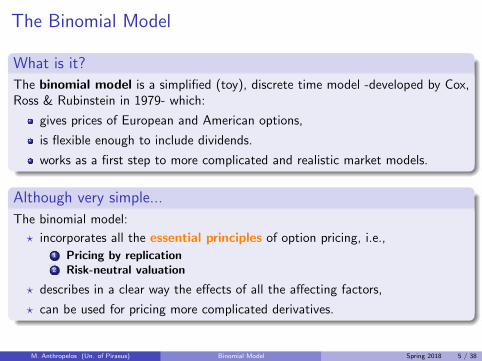
What is it?

The binomial model is a simplified (toy), discrete time model -developed by Cox,Ross & Rubinstein in 1979- which:

gives prices of European and American options,

is flexible enough to include dividends.

works as a first step to more complicated and realistic market models.

Although very simple...

The binomial model:

? incorporates all the essential principles of option pricing, i.e.,1 Pricing by replication2 Risk-neutral valuation

? describes in a clear way the effects of all the affecting factors,

? can be used for pricing more complicated derivatives.


The Stock and the Call OptionThe price of the stock at time t = 0 is S(0). Suppose that at time t = T thereare two possible cases for the stock price:

where, d < 1 + r < u.The situation of a call option written on this stock is the following:


Replication Portfolio

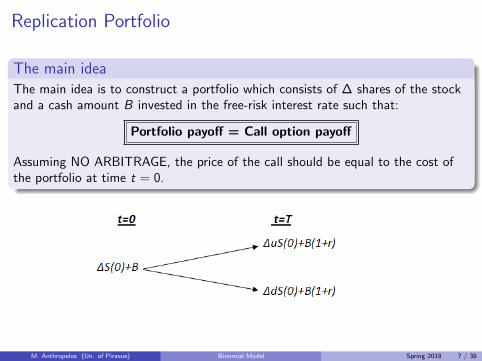
The main ideaThe main idea is to construct a portfolio which consists of ∆ shares of the stockand a cash amount B invested in the free-risk interest rate such that:

Portfolio payoff = Call option payoff

Assuming NO ARBITRAGE, the price of the call should be equal to the cost ofthe portfolio at time t = 0.


Replication Portfolio cont’d

We have to choose ∆ and B such that:

∆uS(0) + B(1 + r) = cu

∆dS(0) + B(1 + r) = cd

If we suppose that, uS(0) > K and dS(0) < K , we have to solve:

∆uS(0) + B(1 + r) = uS(0)− K

∆dS(0) + B(1 + r) = 0

(two linear equations and two unknowns).

Perfect replication

By doing so, we perfectly replicate the call option payoff.


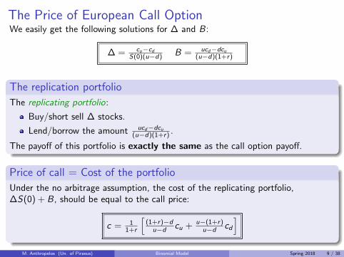
The Price of European Call OptionWe easily get the following solutions for ∆ and B:

∆ = cu−cdS(0)(u−d) B = ucd−dcu

(u−d)(1+r)

The replication portfolio

The replicating portfolio:

Buy/short sell ∆ stocks.

Lend/borrow the amount ucd−dcu(u−d)(1+r) .

The payoff of this portfolio is exactly the same as the call option payoff.

Price of call = Cost of the portfolio

Under the no arbitrage assumption, the cost of the replicating portfolio,∆S(0) + B, should be equal to the call price:

c = 11+r

[(1+r)−d

u−d cu + u−(1+r)u−d cd

]M. Anthropelos (Un. of Piraeus) Binomial Model Spring 2018 9 / 38

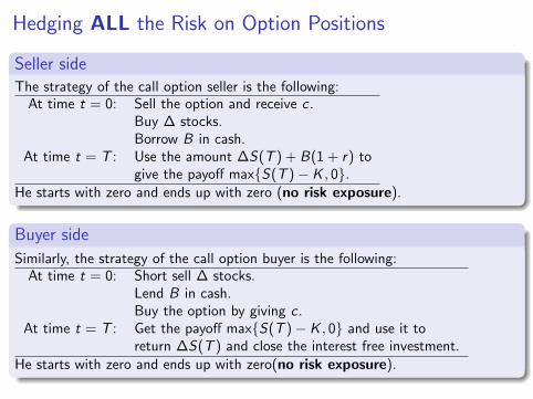
Hedging ALL the Risk on Option Positions

Seller sideThe strategy of the call option seller is the following:

At time t = 0: Sell the option and receive c .Buy ∆ stocks.Borrow B in cash.

At time t = T : Use the amount ∆S(T ) + B(1 + r) togive the payoff max{S(T )− K , 0}.

He starts with zero and ends up with zero (no risk exposure).

Buyer side

Similarly, the strategy of the call option buyer is the following:At time t = 0: Short sell ∆ stocks.

Lend B in cash.Buy the option by giving c .

At time t = T : Get the payoff max{S(T )− K , 0} and use it toreturn ∆S(T ) and close the interest free investment.

He starts with zero and ends up with zero(no risk exposure).

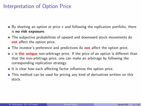
Interpretation of Option Price

By shorting an option at price c and following the replication portfolio, thereis no risk exposure.

The subjective probabilities of upward and downward stock movements donot affect the option price.

The investor’s preference and predictions do not affect the option price.

c is the unique non-arbitrage price. If the price of an option is different thanthat the non-arbitrage price, one can make an arbitrage by following thecorresponding replication strategy.

It is clear how each affecting factor influences the option price.

This method can be used for pricing any kind of derivatives written on thisstock.


Risk-Neutral Valuation

The option price can be written as:

c =1

1 + r

[cu

((1 + r)− d

u − d

)+ cd

(u − (1 + r)

u − d

)].

Note that(

(1+r)−du−d

),(

u−(1+r)u−d

)> 0 and

((1+r)−d

u−d

)+(

u−(1+r)u−d

)= 1.Hence,

c = 11+r [qcu + (1− q)cd ] = 1

1+rEq [C (T )]

In other words, we may consider the option price as the discounted expectation ofthe option payoff, where

the probability of the upward movement of the stock price is given by

q =(

1+r−du−d

)and

the probability of the downward movement is given by 1− q =(

u−1−ru−d

).


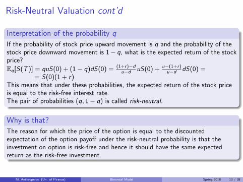
Risk-Neutral Valuation cont’d

Interpretation of the probability q

If the probability of stock price upward movement is q and the probability of thestock price downward movement is 1− q, what is the expected return of the stockprice?

Eq[S(T )] = quS(0) + (1− q)dS(0) = (1+r)−du−d uS(0) + u−(1+r)

u−d dS(0) == S(0)(1 + r)

This means that under these probabilities, the expected return of the stock priceis equal to the risk-free interest rate.The pair of probabilities (q, 1− q) is called risk-neutral.

Why is that?

The reason for which the price of the option is equal to the discountedexpectation of the option payoff under the risk-neutral probability is that theinvestment on option is risk-free and hence it should have the same expectedreturn as the risk-free investment.


Non-Arbitrage and Risk-Neutral Pricing

Synopsis

If the perfect replication of an option payoff is possible, there is no riskinvolved in the option positions and the option price is the uniquenon-arbitrage price.

No risk exposure means that the expected return of the option is equal torisk-free interest rate.

By setting the probabilities of upward and downward movement equal to qand 1− q respectively, we assume that the world is risk-neutral in which:

→ individuals are indifferent to risk.→ the expected return on all securities is the risk-free interest rate.

Important notice

If the perfect replication is possible, the risk-neutral valuation holds not only inthe risk-neutral world but also in the real one.

One Period Binomial Model, an exampleSuppose that the a stock price is $28 today. After one year there are two possibleoutcomes:

A call option written on that stock, with strike price $28 and maturity after oneyear is described below:

One Period Binomial Model, an example

Assume also that r = 5% (annual compounding).The parameters of the replication portfolio are

∆ =cu − cd

S(0)(u − d)=

2.8

28(1.1− 0.9)= 0.5

and

B =ucd − dcu

(u − d)(1 + r)= − 0.9× 2.8

(1.1− 0.9)1.05= −$12.

Hence, the replication strategy is the following:

Borrow $12 at the risk-free rate and

buy 0.5 stocks at the price $28.

The cost of this portfolio is 14− 12 = $2. This means that c = $2.

The risk-neutral probabilities are q = (1+r)−du−d = 1.05−0.9

1.1−0.9 = 0.75 and 1− q = 0.25.Hence, the call option price can also be given by:

c =1

1.05(qcu + (1− q)cd) =

1

1.050.75× 2.8 + 0 = $2.

Outline





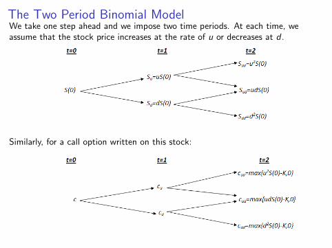
The Two Period Binomial ModelWe take one step ahead and we impose two time periods. At each time, weassume that the stock price increases at the rate of u or decreases at d .

Similarly, for a call option written on this stock:

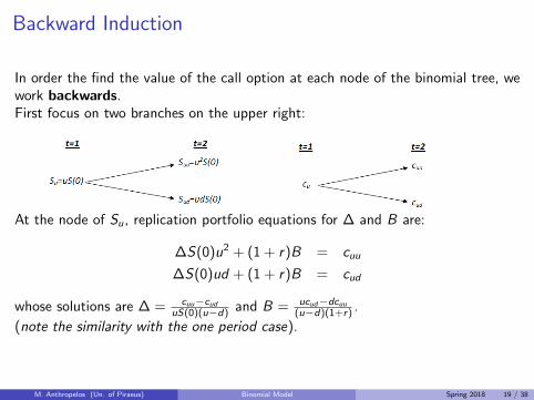
Backward Induction

In order the find the value of the call option at each node of the binomial tree, wework backwards.First focus on two branches on the upper right:

At the node of Su, replication portfolio equations for ∆ and B are:

∆S(0)u2 + (1 + r)B = cuu

∆S(0)ud + (1 + r)B = cud

whose solutions are ∆ = cuu−cuduS(0)(u−d) and B = ucud−dcuu

(u−d)(1+r) .

(note the similarity with the one period case).


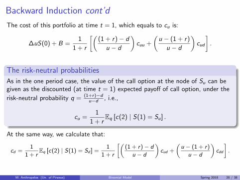
Backward Induction cont’d

The cost of this portfolio at time t = 1, which equals to cu is:

∆uS(0) + B =1

1 + r

[((1 + r)− d

u − d

)cuu +

(u − (1 + r)

u − d

)cud

].

The risk-neutral probabilities

As in the one period case, the value of the call option at the node of Su can begiven as the discounted (at time t = 1) expected payoff of call option, under the

risk-neutral probability q = (1+r)−du−d , i.e.,

cu =1

1 + rEq [c(2) | S(1) = Su] .

At the same way, we calculate that:

cd =1

1 + rEq [c(2) | S(1) = Sd ] =

1

1 + r

[((1 + r)− d

u − d

)cud +

(u − (1 + r)

u − d

)cdd

].


The Price of the Option at Time t = 0

After calculating the option value at time t = 1, we can follow exactly the samemethod in order to value the option at time t = 0. We encounter the followingpart of the binomial tree:

We get:

c =1

(1 + r)Eq[c(1)] =

1

(1 + r)[qcu + (1− q)cd ] =

=1

(1 + r)2[q(qcuu + (1− q)cud) + (1− q)(qcud + (1− q)cdd)] =

=1

(1 + r)2

[q2cuu + 2q(1− q)cud + (1− q)2cdd

]=

=1

(1 + r)2Eq[c(2)].


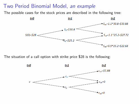
Two Period Binomial Model, an exampleThe possible cases for the stock prices are described in the following tree:

The situation of a call option with strike price $28 is the following:

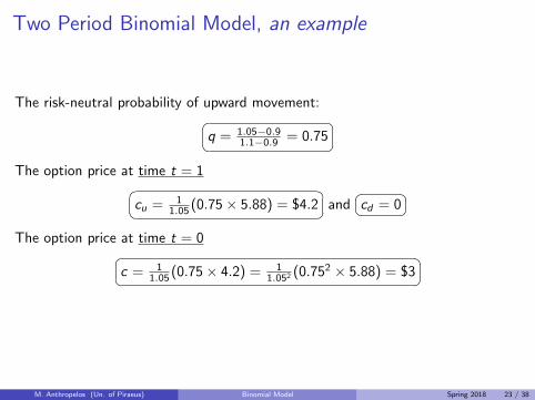
Two Period Binomial Model, an example

The risk-neutral probability of upward movement:�� q = 1.05−0.91.1−0.9 = 0.75

The option price at time t = 1�� cu = 11.05 (0.75× 5.88) = $4.2 and

�� cd = 0

The option price at time t = 0�� c = 11.05 (0.75× 4.2) = 1

1.052 (0.752 × 5.88) = $3


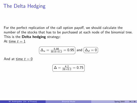
The Delta Hedging

For the perfect replication of the call option payoff, we should calculate thenumber of the stocks that has to be purchased at each node of the binomial tree.This is the Delta hedging strategy:At time t = 1 �� ∆u = 5.88

30.8×0.2 = 0.95 and�� ∆d = 0

And at time t = 0 �� ∆ = 4.228×0.2 = 0.75


The Case of American Options

The ideaFor the price of the American option, we have to take into account the right ofthe option buyer to exercise the option at each node of the binomial tree.Simply, at each node the price of an American option is the maximum betweenthe price of a corresponding European option and the intrinsic option value.In other words, for each note t, we have:�� Ct = max{ct ,S(t)− K} and

�� Pt = max{pt ,K − S(t)}

The early exercise

The early exercise of an American option is optimal if the intrinsic value of theoption is larger than the price of the corresponding European option.


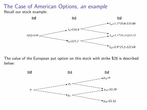
The Case of American Options, an exampleRecall our stock example:

The value of the European put option on this stock with strike $28 is describedbelow:

The Case of American Options, an example

Note that the risk-neutral probability of upward movement remains the same (itdepends on the stock price and the interest rate, but not on the option payoff ):�� q = 1.05−0.9

1.1−0.9 = 0.75

The option price at time t = 1�� pu = 11.05 (0.75× 0 + 0.25× 0.28) = $0.067 and�� pd = 11.05 (0.75× 0.28 + 0.25× 5.32) = $1.467

The option price at time t = 0�� p = 11.05

(0.75 × 0.067 + 0.25 × 1.467) = 11.052 (2 × 0.75 × 0.25 × 0.28 + 0.252 × 5.32) = $0.4


The Case of American Options, an exampleFor the determination of the American put option price at time t = 1, we comparethe two following trees:The tree of the European put option values:

And the tree of the intrinsic option values:

The Case of American Options, an exampleTherefore the price of the American put option at each node of the tree is givenbelow:

At time t = 0, we compare the intrinsic value (=0 in this example) and the value

Eq[P(1)] = q × 0.067 + (1− q)× 2.8 = 0.75025.

The early exercise

At the node Sd , it is optimal for the option holder to exercise the put option andget the payoff of $2.8.


How Dividend Enters the Tree

As we have seen, on the ex-dividend day, the stock price drops by the dividendamount.This decline occurs in two ways:

The dividend is given as a cash amount.

The dividend is given through a continuous dividend yield.


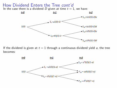
How Dividend Enters the Tree cont’dIn the case there is a dividend D given at time t = 1, we have:

If the dividend is given at t = 1 through a continuous dividend yield a, the treebecomes:

Outline





Starting the Construction of a Tree

How to construct a treeWhen we start the construction of a binomial tree, we have to specify thefollowing parameters:

1 The upward and the downward movement: u and d .

2 The number of the time intervals (periods) which divide the time to maturity.

The more time intervals, the more accuracy we get.

The parameters u and d

The parameters u and d match the stock price volatility.Volatility, , is given by:

Var(Stock return for time period ∆t) = σ2∆t.


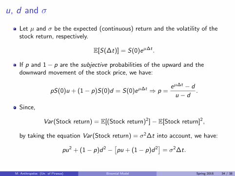
u, d and σ

Let µ and σ be the expected (continuous) return and the volatility of thestock return, respectively.

E[S(∆t)] = S(0)eµ∆t .

If p and 1− p are the subjective probabilities of the upward and thedownward movement of the stock price, we have:

pS(0)u + (1− p)S(0)d = S(0)eµ∆t ⇒ p =eµ∆t − d

u − d.

Since,

Var(Stock return) = E[(Stock return)2]− E[Stock return]2,

by taking the equation Var(Stock return) = σ2∆t into account, we have:

pu2 + (1− p)d2 −[pu + (1− p)d2

]= σ2∆t.


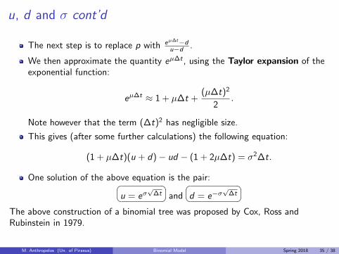
u, d and σ cont’d

The next step is to replace p with eµ∆t−du−d .

We then approximate the quantity eµ∆t , using the Taylor expansion of theexponential function:

eµ∆t ≈ 1 + µ∆t +(µ∆t)2

2.

Note however that the term (∆t)2 has negligible size.

This gives (after some further calculations) the following equation:

(1 + µ∆t)(u + d)− ud − (1 + 2µ∆t) = σ2∆t.

One solution of the above equation is the pair:�� u = eσ√

∆t and

�� d = e−σ√

∆t

The above construction of a binomial tree was proposed by Cox, Ross andRubinstein in 1979.


Facts about the Binomial Tree Construction

F There is a standard and constant relation between u and d :

u ∗ d = 1.

F u and d do not depend on the expected return of the stock price or thesubjective probabilities.

F What matters the most is the volatility of the stock price.

F Volatility and interest rate are constant during the life of the option.


Binomial Tree and Option Pricing, an example

Let’s consider the following example of American put option pricing:

S(0) = 50, K = 50, r = 10% (continuous compounding),σ = 40%, T − t = 5 months = 0.417 and ∆t = 1 month = 0.083

Therefore,

u = eσ√

∆t = 1.224 and d = e−σ√

∆t = 0.891.

And the neutral-risk probability of the upward movement

q = er∆t−du−d = 0.508.


Binomial Tree and Option Pricing, an example

The stock price and the American put option prices are given in the graph of thebinomial tree:


financial derivatives section 4 - unipi.grweb.xrh.unipi.gr/faculty/anthropelos/derivatives/section...

Documents