financial cycles in the euro area: a wavelet...
TRANSCRIPT
Financial cycles in the euro area: a wavelet analysis∗
Michael Scharnagl
Deutsche Bundesbank
Martin Mandler
Deutsche Bundesbank
December 2016
Preliminary and incomplete.
Abstract
We study the relationship of loan to non-financial corporations, loans to house-holds, house prices and equity prices between countries or within countries for nineeuro area countries. Wavelet analysis allows to account for variations in these re-lationships both over time and across frequencies. We find evidence of strong co-movements between the growth rates in loans to non-financial corporations over thesample from 1980 to 2015 for all nine countries. For loans to private households theco-movement increases with the start of EMU. The cycle length is in general shorterthan claimed by the BIS. Equity prices co-move at various frequencies. The degreeof synchronization is in general higher for specific series across the EMU countriesthan across financial series within specific countries.
Keywords: financial cycles, real activity, business cycle, wavelet analysis
JEL classification: C30, E32, E51.
∗Contact address: Deutsche Bundesbank, Wilhelm-Epstein-Strasse 14, D-60431 Frankfurt am Main,Germany. E-Mail: [email protected], [email protected]. This paper rep-resents the authors’ personal opinions and does not necessarily reflect the views of the Deutsche Bundes-bank or its staff.
1
1 Introduction
The financial crisis has led to a renewed interest in macro-financial linkages, with oneimportant aspect being the financial cycle and its possible relationship with cycles in realactivity. A recent literature which has been strongly advanced by researchers from theBIS and IMF has argued for the relevance of financial cycles, i.e. common cycles in variousfinancial variables both within and across countries which operate on lower frequenciesthan business cycles. They have been suggested to represent the build-up of financialimbalances which might culminate in financial crises (Claessens, Kose, and Terrones,2012; Drehmann, Borio, and Tsatsaronis, 2012; Borio, 2014). Empirical analyses suggestthat the length and the amplitude of these financial cycles have increased over time.
A definition of the financial cycle often referred to is that by Borio (2014): ”self-reinforcing interactions between perceptions of value and risk, attitudes towards risk andfinancing constraints, which translate into booms followed by busts”. This kind of rea-soning relates to the pro-cyclicality of the financial system. As the financial cycle is anunobserved variable this concept has to be operationalized. Therefore, a large literatureconcentrates on measurement issues.
Identification of financial cycles has been mainly achieved through the identificationof turning points in time series of financial variables or through the use of statisticalfiltering techniques in order to extract time series components at specific frequencies.The latter approach suffers from selecting the frequency range at which to extract fi-nancial cycles either based upon ex-ante assumptions about the relevant frequency rangeor based on inspection of the spectrum of the financial series which has been estimatedwithout accounting for possible time variation (Aikman, Haldane, and Nelson, 2015). TheBasel committee applies the one-sided HP-filter with a pre-specific smoothing parameter(λ = 400000) based on the credit-to-GDP ratio to measure excessive credit. An alterna-tive approach is applied in Strohsal, Proano, and Wolters (2015) who estimate univariateARMA processes for financial variables and compute their corresponding frequency do-main representations, again, without accounting for possible variation in the relationship.
Wavelet analysis as a tool for time series analysis in the frequency domain can beapplied to estimate dominant frequencies of fluctuations in specific time series as well asthe strength in co-movement among time series. It allows for changes across the frequencyspectrum as well as over time. Furthermore, by computing wavelet cohesion it also beused to study the co-movement of multiple time series with respect to synchronization orsimilarity.
In this paper the relationship between financial variables and real activity is analyzedby wavelet analysis for nine euro area countries. The advantage of this approach isthat there is no need to pre-specify a specific frequency band or turning points. Theanalysis is not restricted to either the time domain or the frequency domain, but usingsimultaneously both approaches. ”Connecting time and frequency analyzes is especiallyrelevant in the current state of the literature, when we have yet to understand the financialcycle and its properties” (Ardila and Sornette, 2016). Section 2 presents a brief overviewof the literature. The applied tools of wavelet methodology are described in Section 3.Empirical results with respect to the duration of cycles, the potential co-movement offinancial cycles and business cycles and the co-movement of financial series are presentedin Section 4. The latter analysis is based on estimating cohesion. This concept was
1
proposed by Croux, Forni, and Reichlin (2001) and applied by Rua and Lopes (2015) inthe context of analyzing the synchronization of business cycles. Section 5 concludes.
2 Literature
The financial cycle can be defined in terms of its duration. In a turning point analysisthe cycle length is measured as the number of periods between two adjacent peaks ortroughs.1 These are a priori defined by a minimum number of periods. This approach isapplied by Claessens et al. (2012) and Drehmann et al. (2012). Claessens et al. (2012)analyze the interaction of financial cycles and business cycles using data for 21 advancedeconomies and 23 emerging market economies from 1960 to 2007. They find that financialvariables (credit, property prices and equity prices) have a greater period and a largeramplitude than real GDP (estimated average length). They find that credit and houseprice cycles are highly synchronized within countries and that recessions that are causedby financial disruptions are longer and deeper. Haavio (2012) combines turning pointanalysis and the calculation of concordance indices for financial variables and real GDPfor 17 OECD countries and finds similar results.
Drehmann et al. (2012) also apply a frequency-based filter (range: 8 to 16 years).Aikman et al. (2015) apply the Christiano-Fitzgerald bandpass filter to analyze the linkbetween the credit cycle and the business cycle. The medium-term frequency is selectedby estimating the spectral densities. They find that the estimated credit cycles havesimilar characteristics as those derived from the turning point analysis.
Koopman and Lucas (2005) and Ruenstler and Vlekke (2016) estimate multivariateunobserved component models for credit, house prices and real GDP. This approach allowsfor testing for similarity of cycle lengths. Ruenstler and Vlekke (2016) find that financialcycles and real GDP are closely related, even at frequencies lower than typical businesscycles frequencies. For US, IT and FR the estimated cycle length is 12 to 15 years. ForUK and ES they are larger and longer, whereas they are very small and short for Germany.
Strohsal et al. (2015) estimate ARMA models to calculate the corresponding spectraldensities. This approach allows for the detection of very long cycles even in the case of alimited sample period. To assess time variation the sample has to be split a priori, as theFourier transform is based on the stationarity of a time series implying the non-existenceof structural breaks. The time series considered are credit, credit-to-GDP, house prices,equity prices and real GDP. For US data they find just a small increase in the period ofreal GDP and equity prices, but a large increase for credit and house prices. For the mostrecent period the duration of the financial cycles in US and UK is around 15 years. ForGermany there is no evidence for a distinct financial cycle.
Verona (2016) applies wavelet methodology to estimate the duration of cycles in credit,house prices, equity prices and GDP for the US. He argues that the financial cycle ismuch longer than the business cycles, although there is spectral power for GDP at similarfrequencies. His conclusion is only valid for credit and house prices, but not for equityprices characterized by higher frequencies. Coherency between financial and real cycles isnot analyzed. In contrast to Strohsal et al. (2015) his results only indicate minor changes
1Ardila and Sornette (2016) propose a wavelet-based estimation of turning points taking uncertaintyinto account. This approach is not applied in this paper as it is based on MODWT.
2

in frequencies over time. Mandler and Scharnagl (2015) show that there is high waveletcoherency of bank-lending and real GDP for Italy and Spain and to a lower degree forFrance even at periods longer than those typically attributed to business cycles. Thesecycles are rather stable over time.
Apart from measuring cycles in individual financial variables, there are some papers oncombining multiple variables into a single measure, i.e. testing whether there are separatecycles in the individual variables (credit cycle, house price cycle, etc.) or whether there issomething like an underlying ”common” financial cycle reflecting the co-movement of the”financial sector”. Drehmann et al. (2012) and Hiebert, Schueler, and Peltonen (2015)estimate cycles for individual variables and average those. Hiebert, Klaus, Peltonen,Schueler, and Welz (2014) estimate individual cycles as well but average those by applyingprincipal component analysis.
3 Wavelet Analysis
Wavelet analysis is an extended form of spectral analysis allowing for time variation.2
Spectral analysis decomposes a time series into a set of cycles with specific periods andestimates the contribution of these cycles to the variance of the series. The co-movementof multiple time series can be analysed at different frequencies. As the underlying trigono-metric functions have infinite support, it is implicitly assumed that the time series arestationary. It is not possible using the estimated spectrum to differentiate between seriesthat are sums of several cycles and series that are characterized by structural changeshaving different sub-sample-specific dominant cycles which is quite common for macroe-conomic time series.
Wavelet analysis is based on finite waves, changes in the importance of specific cyclicalfrequencies can be located in time (Cazelles et al., 2008). Another advantage (also com-pared to rolling window Fourier analysis) is its use of efficient windowing. The windowwidth (sub-sample selection) is scale dependent as the wavelet is stretched or compressed(Aguiar-Conraria, Azevedo, and Soares, 2008).
The continuous wavelet transformation (CWT) is obtained by projecting the timeseries x (t) onto wavelet functions ψ.
Wx (τ, s) =
∞∫
−∞
x (t)1
√
|s|ψ∗
(
t− τ
s
)
dt, (1)
where s represents the scale (”frequency”) and τ the location in time. It is calculatedfor all combinations of scales and time and gives information simultaneously on time andfrequency. High frequency fluctuations imply low values of the scaling factor, while lowfrequency fluctuations imply high values for s. The translation parameter τ controls thelocation of the wavelet, i.e. changes in τ shift the wavelet in time. The function ψ has tofulfil some requirements in order to have the properties of wavelets.3
In the empirical part, the Morlet wavelet is chosen, which is widely used in economic
2This section draws heavily on Aguiar-Conraria and Soares (2014).3For details see, for example Percival and Walden (2002).
3
applications.
ψω0(t) = π− 1
4 eiω0te−t2
2 , (2)
It can be described as a Gaussian modulated sine wave. In its centre it behaves like asine wave, but towards its tails it dies out quite fast (finite support). The Morlet waveletwith ω0 = 6 has optimal joint time-frequency resolution and a direct relation betweenscale and frequency (e.g. Aguiar-Conraria and Soares, 2014, p. 352).
The wavelet power spectrum measures the relative contribution to the variance of thetime series at each scale and at each point in time. It is defined as
WPSx (τ, s) = |Wx (τ, s)|2. (3)
The bigger the wavelet power spectrum WPSx (τi, si), the higher the correlation of thetime series around τi and the wavelet scale si. It will be plotted in a 2-dimensional graph(heat map).
The co-movement of two time series can be estimated by dynamic correlation.
ρxi,xj=
ℜ(
Wxi,xj(τ, s)
)
√
|Wxi(τ, s)|2
√
∣
∣Wxj(τ, s)
∣
∣
2
(4)
where ℜ denotes the real part of the cross-wavelet transform Wxi,xj. The latter is defined
as
Wxi,xj= Wxi
W ∗xj, (5)
where ∗ denotes the complex conjugate. The cross-wavelet transform represents the localcovariance between xi and xj at each time and frequency. Based on dynamic correlationRua and Lopes (2015) propose a measure of cohesion.
coh (τ, s) =
∑
i 6=j
wiwjρxi,xj(τ, s)
∑
i 6=j
wiwj
. (6)
It is a weighted average of all pairwise dynamic correlations (fixed GDP weights).The significance of areas is tested by parametric bootstrap. Based on estimated autore-
gressive processes, a number of simulated replications for each series are generated. Theempirical distribution is based on calculated dynamic correlations for these replications.
To gain deeper insight into divergence between countries, the distances between waveletpower spectra can be analyzed. Following Aguiar-Conraria, Martins, and Soares (2013)wavelet distance matrices are calculated. It can then be tested, whether the estimated
4
similarity is significant.
dist(
Wxi,Wxj
)
=
K∑
k=1
σ2
k
(
d(
lkxi, lkxj
)
+ d(
ukxi, ukxj
))
K∑
k=1
σ2
k
. (7)
The distance matrix dist(
Wxi,Wxj
)
is based on the most important patterns of thewavelet transform (Rouyer, Fromentin, Stensath, and Cazelles, 2008). These are esti-mated via singular value decomposition (maximum covariance analysis).
Wxi≈
K∑
k=1
ukxilkxi
The structure of the distance matrix is then displayed as a cluster tree (dendrogram).Wavelet bandpass filtering is applied to estimate cycles corresponding to specific fre-
quency ranges. This is done by inversion of the wavelet transform of the pre-specifiedinterval.
4 Empirical Results
We use quarterly data for the period from 1980 until the end of 2015 for a series of financialvariables: loans to non-financial corporations (LNFC), loans to private households (LHH),equity prices (EQP) and house prices (HPR). The financial variables are deflated withthe GDP deflator. The data was obtained from the ECB’s statistical warehouse and fromthe BIS (residential property prices). The time series used are annual growth rates. Thisdiffers from other methods applied in the measurement of financial cycles (turning pointanalysis, unobserved component models, etc.). The latter use series in levels. However, thetrends in the levels of the series would lead to spurious coherency and dynamic correlationwhen using spectral analysis. The sample includes data for nine euro area countries:Austria (AT), Belgium (BE), Germany (DE), Spain (ES), Finland (FI), France (FR), Italy(IT), Netherlands (NL) and Portugal (PT). Other member countries are not included asthe approach needs relatively long time series. The lowest frequency to be analyzed isrestricted by the sample length. In some cases, specific variables are not available over thefull sample even for these nine countries: house prices for AT and PT and equity pricesfor PT. These series are then excluded from specific estimations.
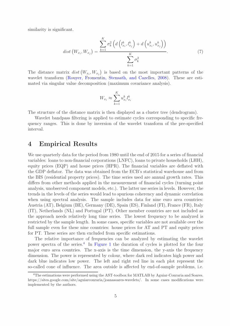
The relative importance of frequencies can be analyzed by estimating the waveletpower spectra of the series.4 In Figure 1 the duration of cycles is plotted for the fourmajor euro area countries. The x-axis is the time dimension, the y-axis the frequencydimension. The power is represented by colour, where dark red indicates high power anddark blue indicates low power. The left and right red line in each plot represent theso-called cone of influence. The area outside is affected by end-of-sample problems, i.e.
4The estimations were performed using the AST-toolbox for MATLAB by Aguiar-Conraria and Soares.https://sites.google.com/site/aguiarconraria/joanasoares-wavelets/. In some cases modifications wereimplemented by the authors.
5
there are not enough data available for calculating the power at specific scales and pointsin time. Corresponding results should not be interpreted as the results might be affectedby zero padding. Loans to non-financial corporations (LNFC) are characterized by cyclesof 10 and 16 years in ES, FR and IT (top panel). These dominant cycles are displayedin the graph as white lines. The durations are relatively stable over time, although thereseems to be a trend towards longer cycles in ES. For Germany there are no long cyclesof 16 years, whereas a shorter cycle of around 6 years is observed. Very short cycles canalso be observed in IT.
DE
LN
FC
1990 2000 2010
36
1016
ES
1990 2000 2010
36
1016
FR
1990 2000 2010
36
1016
IT
1990 2000 2010
36
1016
LH
H
1990 2000 2010
36
1016
1990 2000 2010
36
1016
1990 2000 2010
36
1016
1990 2000 2010
36
1016
HPR
1990 2000 2010
36
1016
1990 2000 2010
36
1016
1990 2000 2010
36
1016
1990 2000 2010
36
1016
EQ
P
1990 2000 2010
36
1016
1990 2000 2010
36
1016
1990 2000 2010
36
1016
1990 2000 2010
36
1016
GD
PR
1990 2000 2010
36
1016
1990 2000 2010
36
1016
1990 2000 2010
36
1016
1990 2000 2010
36
1016
Figure 1: Wavelet power spectra
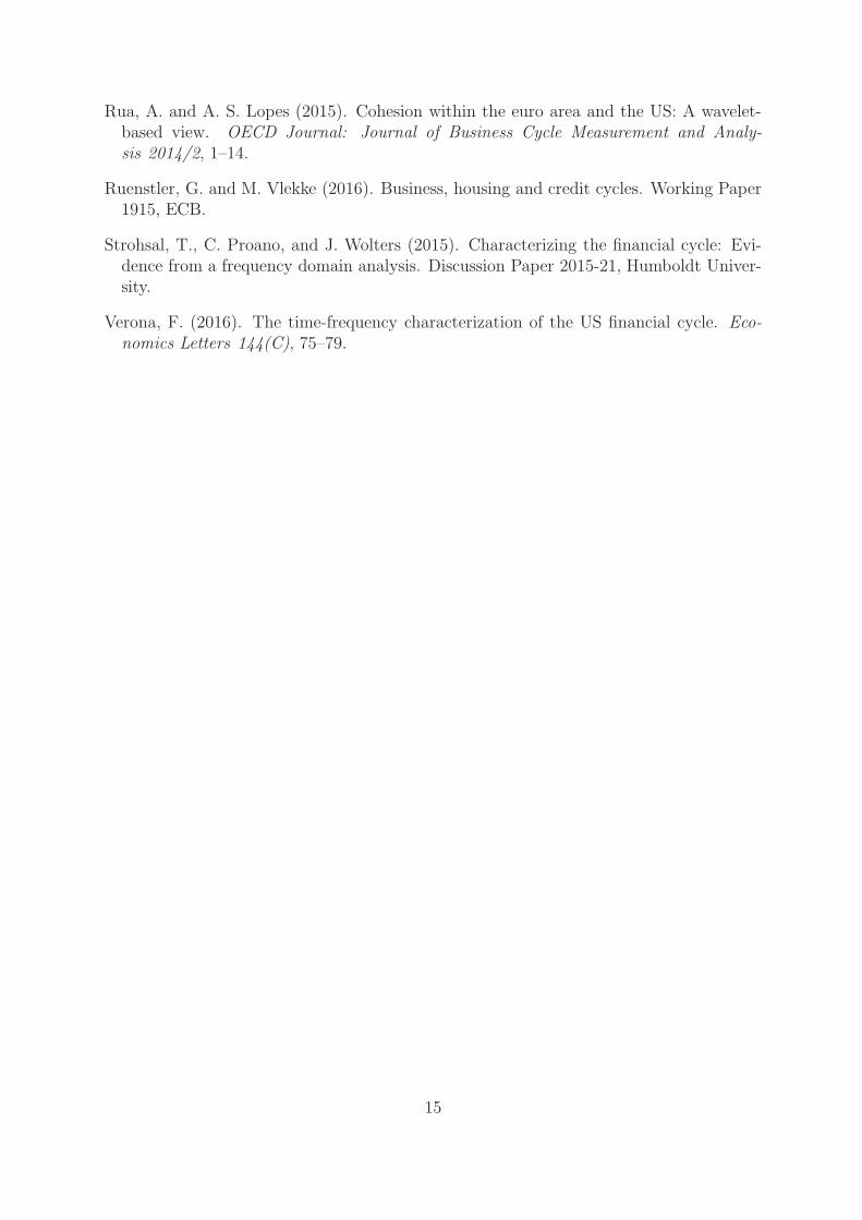
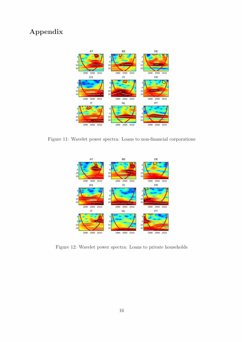
Similar periodicities (10 and 16 years) are estimated for loans to private households(LHH, second panel), with longer cycles showing a tendency to become even longer overtime. Again, the results for DE are different as the low frequency cycle becomes lessimportant after the early 1990s, while the dominant frequency shifts to shorter cycles. Thepower of house prices (third panel) is for most countries mainly in the lower frequenciesaround 14 to 16 years in ES, FR and IT and show a tendency to longer cycles as did loans tohouseholds. For DE the results indicate an important cycle at a somewhat lower frequencybut also a cycle with fluctuations of about ten years which weakens and disappears afterthe late 1990s. The results for the other countries (shown in the appendix) are similar tothose for the large countries shown here with the power spectra for some countries andvariables more similar to ES, FR and IT or more similar to DE (e.g. NL and AT).
6
The wavelet power spectra for equity prices (fourth panel) are in stark contrast tothose for the other financial series with various dominant frequencies within each countrycovering most of the frequency spectrum. Except for IT which also exhibits importantcycles with duration of 16 years, the cycles tend to shorter fluctuations compared to loansand house prices.
The bottom panel shows the spectra for real GDP. The comparison to those for theother series might give a first impression of potential co-movements of financial variablesand real activity. With the exception of DE, periodicities in loans and real GDP seem tobe similar at 10 and 16 years while for DE only the shorter cycle of six years seems tobe reflected in loans and real GDP. The results also suggest co-movement in real outputgrowth and house prices in ES, FR and IT at low frequencies. In contrast there seems tobe less similarity in fluctuations in equity prices and real output.
DE
LN
FC
1990 2000 2010
3
61016
ES
1990 2000 2010
3
61016
FR
1990 2000 2010
3
61016
IT
1990 2000 2010
3
61016
LH
H
1990 2000 2010
3
61016
1990 2000 2010
3
61016
1990 2000 2010
3
61016
1990 2000 2010
3
61016
HPR
1990 2000 2010
3
61016
1990 2000 2010
3
61016
1990 2000 2010
3
61016
1990 2000 2010
3
61016
EQ
P
1990 2000 2010
3
61016
1990 2000 2010
3
61016
1990 2000 2010
3
61016
1990 2000 2010
3
61016
Figure 2: Cohereny of LNFC, LHH, HPR and EQP with real GDP for EA4
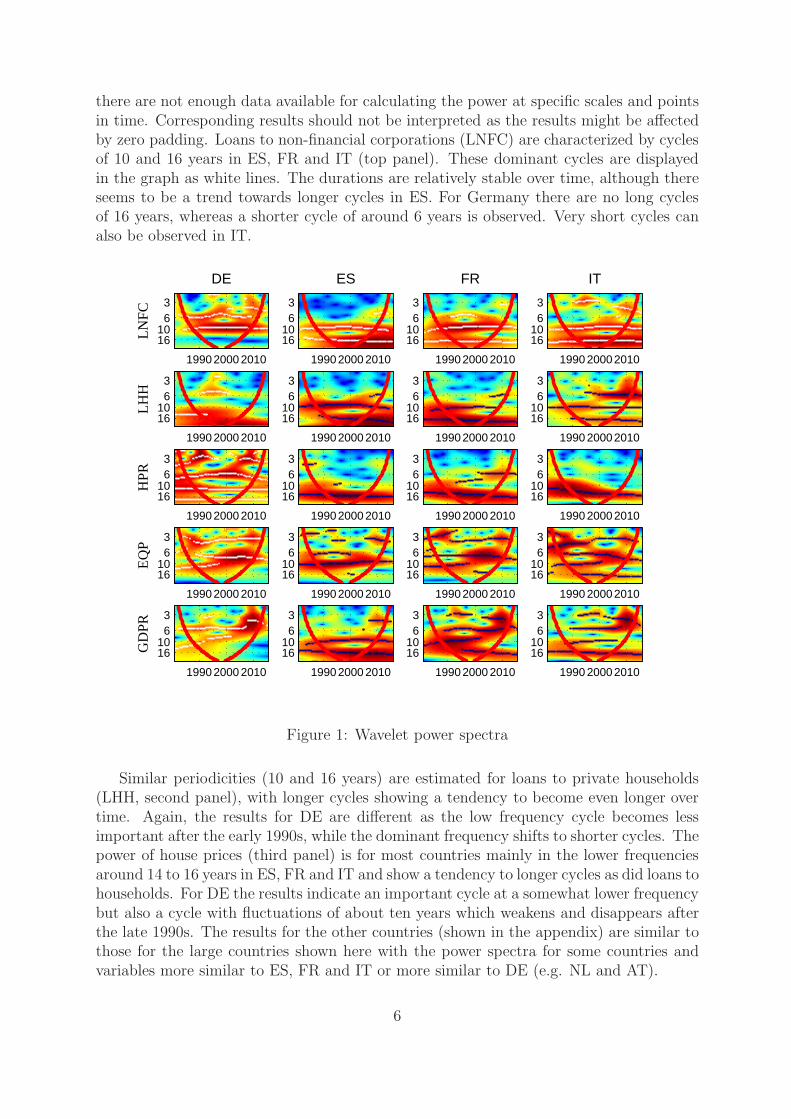
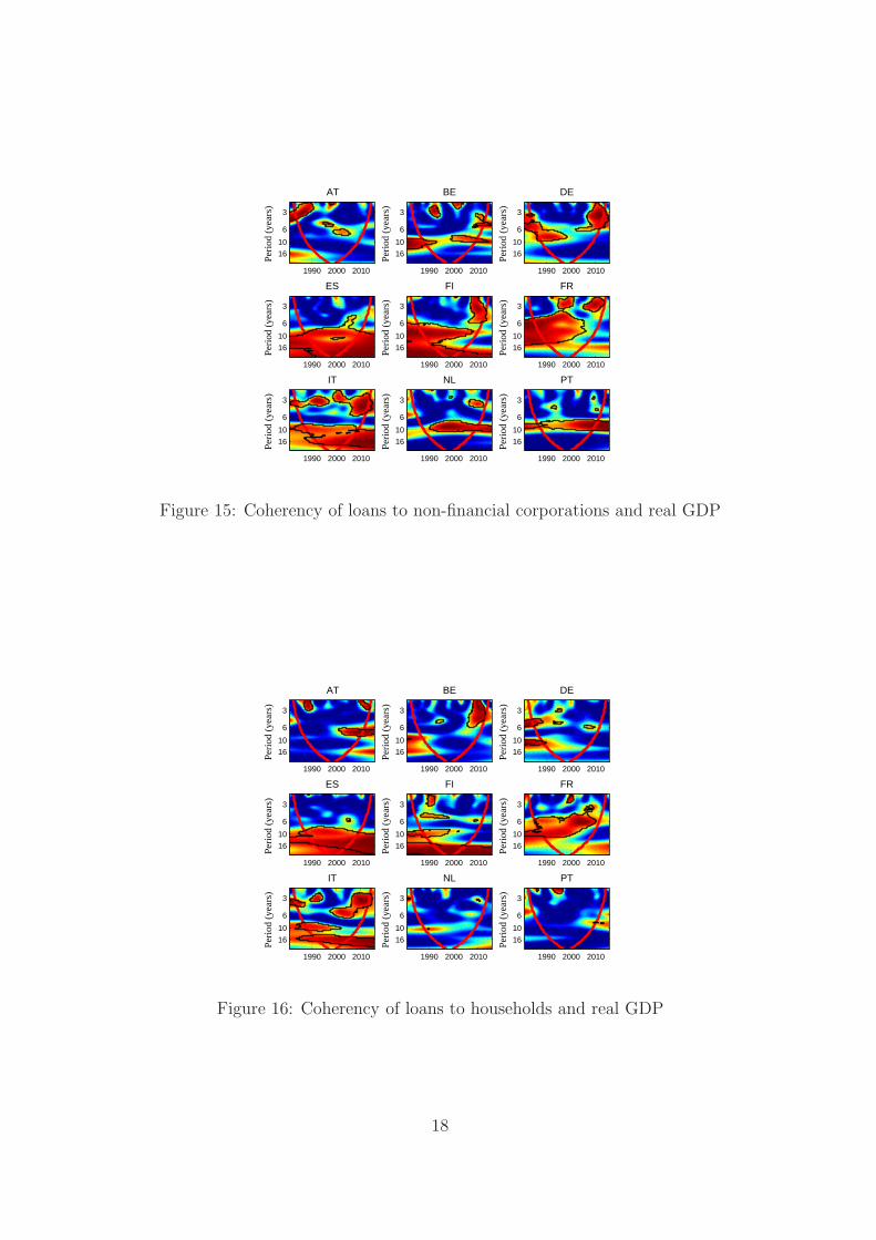
Figure 2 shows the coherency between loans, house prices, equity prices and real GDPwhich provides information on the co-movement between the financial variables and realactivity. The panels show the level of coherency which falls between zero (dark blue)and one (dark red) with the black lines indicating significance at the 5% level.5 Thecurved red lines indicate the cone of influence. Loans to non-financial corporations andreal GDP (top panel) show high coherency for cycles with a duration of between six andten years in ES and IT throughout the sample period. In FR, initially, coherency is large
5Results for all nine countries are in the appendix.
7
and significant across a broad frequency band, but weakens after the mid-2000s. Similarto the results for the wavelet power spectrum high coherency in DE is not estimated atlonger durations but significant coherency is obtained at cycles with periodicities of sixto ten years and is not stable over time. The results for lending to households (secondrow) are broadly similar with a narrower range of frequencies with significant coherencies.Again for ES and IT significant and stable coherency is estimated at low frequencies. ForFR we estimate significant coherency for cycles with duration of between six and yearsbut with a tendency to the shorter end of this frequency spectrum over the 2000s. ForDE, however, we find no evidence of stable co-movements between loans to householdsand real activity at any frequency. Coherency between house prices and real GDP (thirdrow) is close to one and stable in ES and FR at periodicities around 16 years. For DEthere is no evidence of significant co-movements between real GDP and real house pricesat any frequency and for IT only in the late 1980s and early 1990s. Finally, for realequity prices significant coherency is estimated in FR and IT for cycles with durations often to 16 years and around 16 years, respectively. For ES coherency is only temporarilysignificant at higher frequencies and for DE coherency is generally relatively low.
Overall, these results indicate for many countries significant relationships betweenmedium or long-run cycles in financial variables and real activity. However, there are alsoimportant cross-country differences, such as the weak correlations between these cycles inDE.
LNFC
Peri
od (
year
s)
1990 2000 2010
3
6
10
16
LHH
Peri
od (
year
s)
1990 2000 2010
3
6
10
16
HPR
Peri
od (
year
s)
1990 2000 2010
3
6
10
16
EQP
Peri
od (
year
s)
1990 2000 2010
3
6
10
16
−1 −0.5 0 0.5 1
Figure 3: Cohesion across all countries
8

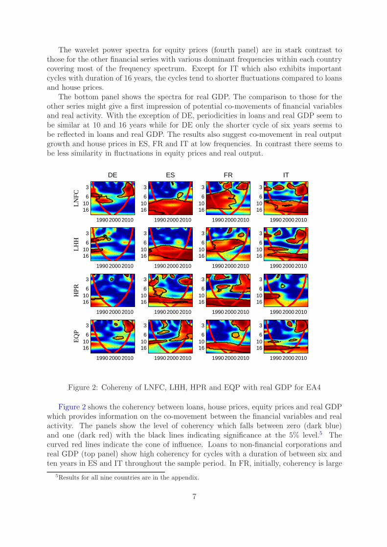
Figure 3 shows the estimated cohesion for these four financial variables, i.e. thestrength of the cross-country dynamic correlation. For each variable the cohesion measureis computed as GDP weighted average of the dynamic correlations between all countrypairs. Here, all nine countries (seven in the case of real house prices and eight in thecase of equity prices) are considered. By construction, cohesion is restricted to the in-terval between minus one (dark blue) and plus one (dark red). Green indicates cohesionaround zero, i.e. no contemporaneous correlation on average across countries. For loansto non-financial corporations (top row, left) cohesion is close to one in the frequencyrange between six and ten years over the full sample suggesting a stable common cycleamong euro area countries in this frequency range. At higher frequencies we also esti-mate increasing cohesion after the introduction of EMU. For loans to households (toprow, right) cohesion is much lower until the late 1990s when it becomes significant overa widening frequency band. The dominant cycles in loans to households with durationsof six and ten years thus do not display strong correlations across countries. In contrast,the co-movements are at higher frequencies. Real house prices (bottom row, left) displaymoderate and not significant cohesion for cycles with duration of six years and more in thelate 1990s but then weakens over time. The estimates indicate a significant co-movementof house prices at low frequencies up to 2000 as highlighted in Figure 1. In contrast,cross-country cohesion of equity prices (bottom row, right) is large and significant foralmost the full sample period and across all frequencies. Overall, these results suggestcommon cycles in the lending to non-financial corporations, households (for part of thesample) and real equity prices while there is little evidence of a common house price cycleat the end of the sample.
Real GDP
Peri
od (
year
s)
1990 2000 2010
3
6
10
16
−1 −0.8 −0.6 −0.4 −0.2 0 0.2 0.4 0.6 0.8 1
Figure 4: Cohesion of real GDP across all countries
For comparison Figure 4 shows the estimated cohesion for real GDP, i.e. synchro-nisation of real activity. We find persistently high cohesion for cycles with duration of
9

about 10 and 16 years which were shown to be dominant frequencies in the wavelet powerspectrum for many countries. Cohesion also attains high values at higher frequencies andthe degree of synchronisation of output growth at these higher frequencies has becomemore pronounced after the 1990s. Thus, the estimated cohesion for the financial vari-ables – with the exception of equity prices – indicates a more narrow frequency range ofco-movements in bank lending and house prices than of co-movements in real activity.
The high cohesion of loans to non-financial corporations is reflected by relatively lowdistances between the wavelet spectra of different countries. Figure 5 shows this measurefor frequencies between 6 and 16 years by means of a dendrogram (left panel). The smallerthe value, the higher the similarity of the corresponding cycles. Cycles for BE and NL aswell as those for ES and IT are quite closely linked. Those of FI and AT are further apartfrom the rest of the group as is also visible for the filtered series generated by inversionof the wavelet transform (right panel).
BE NL FR PT ES IT DE FI AT
0.1
0.15
0.2
0.25
0.3
0.35
Dis
tanc
es
1980 1990 2000 2010 2020-3
-2
-1
0
1
2
3 ATBEDEESFIFRITNLPT
Figure 5: Distances and filtered series: LNFC, 6 to 16 years
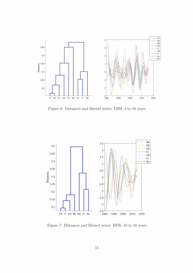
Synchronization of loans to private households changes over time (Figure 6). Up tomid90s the time series evolve quite differently. From then onwards the co-movementbecomes stronger. This is also reflected in the cohesion (upper right panel of Figure 3).Due to low synchronization in the 80s and early 90s the values of the estimated distancesare considerably larger than those of loans to non-financial corporations as these areaverages over the full sample. Starting in 2000 the co-movement of the filtered series inthe frequency range from 4 to 10 years is much higher than before (right panel).
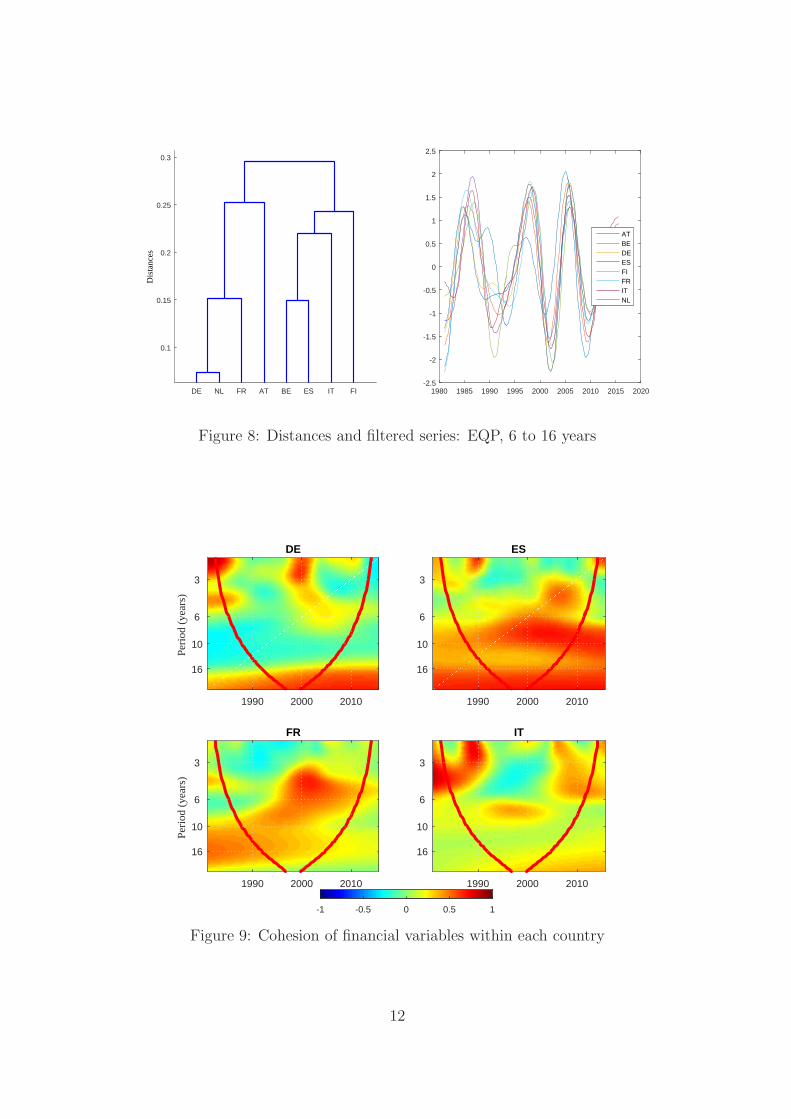
Reflecting the differences in cohesion for house prices and equity prices Figure 7 andFigure 8 show cross-country differences in distances and filtered series. Apart from somedisturbances in the first half of the 90s the cycles in equity prices are highly synchronized.
Cohesion within a specific country is calculated as an un-weighted average of thedynamic correlations of all possible combinations (Figure 9). The correlation of cycles ofall financial variables within DE is in general quite low. This picture is similar to thoseof FR and IT. For ES there is some correlation in the 2000s.
Adding further financial variables (long-term interest rate, spread between the long-term bond yield and the short-term rate and growth rate of M3) potentially reflecting a
10
FI FR NL ES PT BE AT IT DE
0.3
0.35
0.4
0.45
0.5
0.55
Dis
tanc
es
1980 1990 2000 2010 2020-3
-2
-1
0
1
2
3
4ATBEDEESFIFRITNLPT
Figure 6: Distances and filtered series: LHH, 4 to 10 years
FR IT ES BE DE FI NL
0.1
0.15
0.2
0.25
0.3
0.35
0.4
0.45
0.5
Dis
tanc
es
1980 1990 2000 2010 2020-2.5
-2
-1.5
-1
-0.5
0
0.5
1
1.5
2
2.5BEDEESFIFRITNL
Figure 7: Distances and filtered series: HPR, 10 to 16 years
11
DE NL FR AT BE ES IT FI
0.1
0.15
0.2
0.25
0.3D
ista
nces
1980 1985 1990 1995 2000 2005 2010 2015 2020-2.5
-2
-1.5
-1
-0.5
0
0.5
1
1.5
2
2.5
ATBEDEESFIFRITNL
Figure 8: Distances and filtered series: EQP, 6 to 16 years
DE
1990 2000 2010
3
6
10
16
Peri
od (
year
s)
ES
1990 2000 2010
3
6
10
16
FR
1990 2000 2010
3
6
10
16
Peri
od (
year
s)
IT
1990 2000 2010
3
6
10
16
-1 -0.5 0 0.5 1
Figure 9: Cohesion of financial variables within each country
12
DE
1990 2000 2010
3
6
10
16
Peri
od (
year
s)
ES
1990 2000 2010
3
6
10
16
FR
1990 2000 2010
3
6
10
16
Peri
od (
year
s)
IT
1990 2000 2010
3
6
10
16
-1 -0.5 0 0.5 1
Figure 10: Cohesion of (seven) financial variables within each country
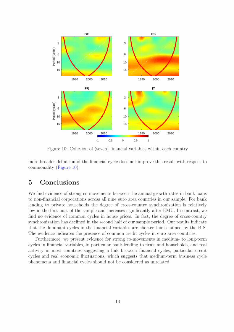
more broader definition of the financial cycle does not improve this result with respect tocommonality (Figure 10).
5 Conclusions
We find evidence of strong co-movements between the annual growth rates in bank loansto non-financial corporations across all nine euro area countries in our sample. For banklending to private households the degree of cross-country synchronization is relativelylow in the first part of the sample and increases significantly after EMU. In contrast, wefind no evidence of common cycles in house prices. In fact, the degree of cross-countrysynchronization has declined in the second half of our sample period. Our results indicatethat the dominant cycles in the financial variables are shorter than claimed by the BIS.The evidence indicates the presence of common credit cycles in euro area countries.
Furthermore, we present evidence for strong co-movements in medium- to long-termcycles in financial variables, in particular bank lending to firms and households, and realactivity in most countries suggesting a link between financial cycles, particular creditcycles and real economic fluctuations, which suggests that medium-term business cyclephenomena and financial cycles should not be considered as unrelated.
13
References
Aguiar-Conraria, L., N. Azevedo, and M. Soares (2008). Using wavelets to decompose thetime-frequency effects of monetary policy. Physica A 387, 2863–2878.
Aguiar-Conraria, L., M. Martins, and M. Soares (2013). Convergence of the economicsentiment cycles in the eurozone: a time-frequency analysis. Journal of Common MarketStudies 51:3, 377–398.
Aguiar-Conraria, L. and M. Soares (2014). The continuous wavelet transform: movingbeyond uni- and bivariate analysis. Journal of Economic Surveys 28:2, 344–375.
Aikman, D., A. Haldane, and B. Nelson (2015). Curbing the credit cycle. The EconomicJournal 125(585), 1072–1109.
Ardila, D. and D. Sornette (2016). Dating the financial cycle with uncertainty estimates:a wavelet proposition. Finance Research Letters 19, 298–304.
Borio, C. (2014). The financial cycle and macroeconomics: What have we learnt? Journalof Banking and Finance 45C, 182–198.
Claessens, S., A. Kose, and M. Terrones (2012). How do business and financial cyclesinteract? Journal of International Economics 87, 178–190.
Croux, C., M. Forni, and L. Reichlin (2001). A measure of comovement for economicvariables: theory and empirics. Review of Economics and Statistics 83:2, 232–241.
Drehmann, M., C. Borio, and K. Tsatsaronis (2012). Characterising the financial cycle:don’t lose sight of the medium term! Working Paper 380, Bank for InternationalSettlements.
Haavio, M. (2012). Financial cycles and business cycles: some stylized facts. BoF Online1.2012, Bank of Finland.
Hiebert, P., B. Klaus, T. Peltonen, Y. Schueler, and P. Welz (2014). Capturing thefinancial cycle in euro area countries. Financial stability review, ECB.
Hiebert, P., Y. Schueler, and T. Peltonen (2015). Characterizing the financial cycle: amultivariate and time-varying approach. Working Paper 1846, ECB.
Koopman, S. and A. Lucas (2005). Business and default cycles for credit risk. Journal ofApplied Econometrics 20:2, 311–323.
Mandler, M. and M. Scharnagl (2015). Bank lending to non-financial corporations andthe real economy: a wavelet analysis. mimeo, Deutsche Bundesbank.
Percival, D. and A. Walden (2002). Wavelet Methods for Time Series Analysis. CambridgeUniversity Press.
Rouyer, T., J.-M. Fromentin, N. Stensath, and B. Cazelles (2008). Analyzing multiple timeseries and extending significance testing in wavelet analysis. Marine Ecology ProgressSeries 359, 11–23.
14
Rua, A. and A. S. Lopes (2015). Cohesion within the euro area and the US: A wavelet-based view. OECD Journal: Journal of Business Cycle Measurement and Analy-sis 2014/2, 1–14.
Ruenstler, G. and M. Vlekke (2016). Business, housing and credit cycles. Working Paper1915, ECB.
Strohsal, T., C. Proano, and J. Wolters (2015). Characterizing the financial cycle: Evi-dence from a frequency domain analysis. Discussion Paper 2015-21, Humboldt Univer-sity.
Verona, F. (2016). The time-frequency characterization of the US financial cycle. Eco-nomics Letters 144(C), 75–79.
15
Appendix
AT
1990 2000 2010
3
6
10
16
BE
1990 2000 2010
3
6
10
16
DE
1990 2000 2010
3
6
10
16
ES
1990 2000 2010
3
6
10
16
FI
1990 2000 2010
3
6
10
16
FR
1990 2000 2010
3
6
10
16
IT
1990 2000 2010
3
6
10
16
NL
1990 2000 2010
3
6
10
16
PT
1990 2000 2010
3
6
10
16
Figure 11: Wavelet power spectra: Loans to non-financial corporations
AT
1990 2000 2010
3
6
10
16
BE
1990 2000 2010
3
6
10
16
DE
1990 2000 2010
3
6
10
16
ES
1990 2000 2010
3
6
10
16
FI
1990 2000 2010
3
6
10
16
FR
1990 2000 2010
3
6
10
16
IT
1990 2000 2010
3
6
10
16
NL
1990 2000 2010
3
6
10
16
PT
1990 2000 2010
3
6
10
16
Figure 12: Wavelet power spectra: Loans to private households
16

BE
1990 2000 2010
3
6
10
16
DE
1990 2000 2010
3
6
10
16
ES
1990 2000 2010
3
6
10
16
FI
1990 2000 2010
3
6
10
16
FR
1990 2000 2010
3
6
10
16
IT
1990 2000 2010
3
6
10
16
NL
1990 2000 2010
3
6
10
16
Figure 13: Wavelet power spectra: House prices
AT
1990 2000 2010
3
6
10
16
BE
1990 2000 2010
3
6
10
16
DE
1990 2000 2010
3
6
10
16
ES
1990 2000 2010
3
6
10
16
FI
1990 2000 2010
3
6
10
16
FR
1990 2000 2010
3
6
10
16
IT
1990 2000 2010
3
6
10
16
NL
1990 2000 2010
3
6
10
16
Figure 14: Wavelet power spectra: Equity prices
17
AT
Peri
od (
year
s)
1990 2000 2010
3
6
10
16
BE
Peri
od (
year
s)
1990 2000 2010
3
6
10
16
DE
Peri
od (
year
s)
1990 2000 2010
3
6
10
16
ES
Peri
od (
year
s)
1990 2000 2010
3
6
10
16
FI
Peri
od (
year
s)
1990 2000 2010
3
6
10
16
FR
Peri
od (
year
s)
1990 2000 2010
3
6
10
16
IT
Peri
od (
year
s)
1990 2000 2010
3
6
10
16
NLPe
riod
(ye
ars)
1990 2000 2010
3
6
10
16
PT
Peri
od (
year
s)
1990 2000 2010
3
6
10
16
Figure 15: Coherency of loans to non-financial corporations and real GDP
AT
Peri
od (
year
s)
1990 2000 2010
3
6
10
16
BE
Peri
od (
year
s)
1990 2000 2010
3
6
10
16
DE
Peri
od (
year
s)
1990 2000 2010
3
6
10
16
ES
Peri
od (
year
s)
1990 2000 2010
3
6
10
16
FI
Peri
od (
year
s)
1990 2000 2010
3
6
10
16
FR
Peri
od (
year
s)
1990 2000 2010
3
6
10
16
IT
Peri
od (
year
s)
1990 2000 2010
3
6
10
16
NL
Peri
od (
year
s)
1990 2000 2010
3
6
10
16
PT
Peri
od (
year
s)
1990 2000 2010
3
6
10
16
Figure 16: Coherency of loans to households and real GDP
18

BE
Peri
od (
year
s)
1990 2000 2010
3
6
10
16
DE
Peri
od (
year
s)
1990 2000 2010
3
6
10
16
ES
Peri
od (
year
s)
1990 2000 2010
3
6
10
16
FI
Peri
od (
year
s)
1990 2000 2010
3
6
10
16
FR
Peri
od (
year
s)
1990 2000 2010
3
6
10
16
IT
Peri
od (
year
s)
1990 2000 2010
3
6
10
16
NLPe
riod
(ye
ars)
1990 2000 2010
3
6
10
16
Figure 17: Coherency of house prices and real GDP
AT
Peri
od (
year
s)
1990 2000 2010
3
6
10
16
BE
Peri
od (
year
s)
1990 2000 2010
3
6
10
16
DE
Peri
od (
year
s)
1990 2000 2010
3
6
10
16
ES
Peri
od (
year
s)
1990 2000 2010
3
6
10
16
FI
Peri
od (
year
s)
1990 2000 2010
3
6
10
16
FR
Peri
od (
year
s)
1990 2000 2010
3
6
10
16
IT
Peri
od (
year
s)
1990 2000 2010
3
6
10
16
NL
Peri
od (
year
s)
1990 2000 2010
3
6
10
16
Figure 18: Coherency of equity prices and real GDP
19