financial crises and systemic bank runs in a dynamic model ...€¦ · financial crises and...
TRANSCRIPT

Working Paper Series
n. 62 ■ December 2014
Financial Crises and Systemic Bank Runs in a Dynamic Model of Banking
Roberto Robatto

1 WORKING PAPER SERIES N. 62 -DECEMBER 2014 ■
Statement of Purpose
The Working Paper series of the UniCredit & Universities Foundation is designed to disseminate and
to provide a platform for discussion of either work of UniCredit economists and researchers or outside
contributors (such as the UniCredit & Universities scholars and fellows) on topics which are of special
interest to UniCredit. To ensure the high quality of their content, the contributions are subjected to an
international refereeing process conducted by the Scientific Committee members of the Foundation.
The opinions are strictly those of the authors and do in no way commit the Foundation and UniCredit
Group.
Scientific Committee
Franco Bruni (Chairman), Silvia Giannini, Tullio Jappelli, Levent Kockesen, Christian Laux; Catherine
Lubochinsky, Massimo Motta, Giovanna Nicodano, Marco Pagano, Reinhard H. Schmidt, Branko
Urosevic.
Editorial Board
Annalisa Aleati
Giannantonio De Roni
The Working Papers are also available on our website (www.unicreditanduniversities.eu)

2 WORKING PAPER SERIES N. 62 -DECEMBER 2014 ■
Contents
Abstract 3
1. Introduction 4
2. Model 9
3. Equilibrium 13
4. Results 21
5. Monetary policy 28
6. Conclusions 33

3 WORKING PAPER SERIES N. 62 -DECEMBER 2014 ■
Financial Crises and Systemic Bank Runs in a Dynamic Model of Banking
Roberto Robatto
Department of Finance, University of Wisconsin-Madison
Abstract
I present a new dynamic general equilibrium model of banking to analyze monetary policy during
financial crises. A novel channel gives rise to multiple equilibria. In the good equilibrium, all banks are
solvent. In the bad equilibrium, many banks are insolvent and subject to runs. The bad equilibrium is
also characterized by deflation and a flight to liquidity. Some central bank interventions are more
effective than others at eliminating the bad equilibrium. Interventions that do not eliminate the bad
equilibrium still counteract deflation and reduce the losses of insolvent banks, but, for some parameter
values, amplify the flight to liquidity.
JEL codes: E44, E52, G0], G2]
University of Wisconsin-Madison, Wisconsin School of Business, 975 University Avenue, Madison WI 53706. E-mail: [email protected]. This paper is based on the main chapter of my Ph.D. dissertation at the University of Chicago. I am grateful to Fernando Alvarez, Veronica Guerrieri, Robert Lucas, and Harald Uhlig for suggestions and guidance, and to Ana Babus, Gadi Barlevy, Philip Barrett, Martin Beraja, Maryam Farboodi, Kinda Hachem, Lars Hansen, Rebecca Myerson, Stefanie Stantcheva, Balázs Szentes, Pietro Veronesi, seminar participants at BFI Financial Markets and Contracts Graduate Student Conference, Chicago Fed, EIEF, Federal Reserve Board, Macro-Financial Modeling Group Meetings, Richmond Fed, University of Chicago, University of Toronto and University of Wisconsin-Madison for comments. I thank the Becker-Friedman Institute and the Macroeconomic Modeling and Systemic Risk Research Initiative for financial support.

4 WORKING PAPER SERIES N. 62 -DECEMBER 2014 ■
1. Introduction
A peculiar event of the 2007-2009 US financial crisis was a dramatic increase in the private sector’s
willingness to hold liquid assets, a “flight to liquidity.” The Federal Reserve reacted aggressively at the
time, implementing unconventional monetary policies. The flight to liquidity and the interventions of the
Fed resulted in an approximately constant price level and a sizable drop in the money multiplier.1 The
Great Depression saw a similar drop in the money multiplier. Friedman and Schwartz (1963) argue
that the absence of adequate Federal Reserve intervention at that time generated deep deflation,
making what would otherwise have been a modest or deep recession the Great Depression.
During both these crises, several financial institutions became insolvent and were subject to runs.
More than one-fifth of the commercial banks in the US suspended operations during the Great
Depression (Friedman and Schwartz, 1963). The collapse of Lehman Brothers in September 2008
was followed by a “run on repo” and on other institutions not covered by deposit insurance, as Gorton
and Metrick (2012a,b) document.
Motivated by these events, the first contribution of this paper is to provide a new dynamic general
equilibrium model of banking with multiple equilibria. The multiplicity of equilibria is based on a debt-
deflation channel similar to Fisher (1933), a novel approach in the panic-based bank runs literature. In
the good equilibrium, all banks are solvent. In the bad equilibrium, many banks are insolvent and
subject to runs. Distress in the banking sector is associated with deflation, a drop in asset prices, and
a flight to liquidity (that is, depositors hold more money and fewer deposits at banks, in comparison to
the good equilibrium). In the model, runs and insolvencies are systemic events, in the sense that many
financial institutions are subject to distress at the same time. Therefore, the model captures the
systemic nature of financial crises.
The second contribution is an application of the model to analyze some of the monetary policies used
during the recent US financial crisis. In the model, a central bank can inject money into the economy
by either 1) buying assets on the market (asset purchases), or 2) setting up liquidity facilities (in order
to provide loans to banks). Using numerical simulations of the model, I show that both asset
purchases and loans to banks counteract deflation, reduce the losses of insolvent banks, and if the
intervention of the central bank is sufficiently large, eliminate the bad equilibrium. This result is
consistent with the Friedman-Schwartz hypothesis regarding the Great Depression. In addition, there
are two novel results. First, in some circumstances loans to banks eliminate the bad equilibrium while
asset purchases do not. Second, for some parameter values, if a temporary monetary injection does
not eliminate the bad equilibrium, it amplifies the flight to liquidity.
In the model, households are subject to uninsurable preference shocks that affect the utility of
consumption, similarly to Diamond and Dybvig (1983). There is an exogenous supply of two assets in
the economy, fiat money and a productive asset (capital). Trading frictions interact with the timing of
preference shocks and create a precautionary demand for money to finance consumption expenditure. 1 The money multiplier is the ratio of broad monetary aggregates, such as M1 or M2, to the monetary base M0.

5 WORKING PAPER SERIES N. 62 -DECEMBER 2014 ■
Banks offer deposits in order to provide money to households on demand. In the model, banks are
unregulated institutions that perform maturity transformation without deposit insurance, similar to
commercial banks in the 1930s and to the shadow banking system in recent years.
In the banking sector, two frictions are crucial. First, deposits are nominal, i.e., specified in terms of
money. Second, capital held by banks is hit by idiosyncratic shocks (in particular, I will consider one-
time unanticipated shocks). For an individual bank, a negative shock destroys some of its capital,
while a positive shock increases its stock of capital. Since the shocks are idiosyncratic, the aggregate
stock of capital is constant. Crucially, there is asymmetric information about the shocks. Each bank
observes its own shock, but it takes time for other banks and households to observe them. Thus,
households do not know whether their own bank has been hit by a positive or a negative shock.2
In a steady-state with no shocks to banks, deposits overcome the frictions that give rise to the
precautionary demand for money. When the one-time unanticipated shocks hit banks, a good
equilibrium always exists wherein all banks are solvent (including banks hit by a negative shock) and
the banking sector functions normally as in steady-state. A bad equilibrium exists for a large subset of
the parameter space. The bad equilibrium lasts one period and then the economy reverts to normal.
However, the model can be extended so that the bad equilibrium lasts many periods.
A bad equilibrium is characterized by three features. First, the economy experiences deflation and a
drop in the nominal price of capital. Second, a bank hit by a negative shock becomes insolvent; the
value of capital drops due to the drop in its nominal price and to the negative idiosyncratic shock, while
liabilities (deposits) are in nominal terms and thus constant (debt-deflation). Banks hit by a positive
shock remain solvent. Asymmetric information prevents depositors from immediately identifying
insolvent banks, but eventually, the insolvency of banks becomes common knowledge and insolvent
banks are subject to runs. Third, anticipating the possibility of runs, households hold more money and
fewer deposits due to the precautionary demand for money (flight to liquidity).
This scenario is an equilibrium because there is a general equilibrium feedback from the flight to
liquidity to the drop in prices. With the flight to liquidity, some money is stored under the mattress for
precautionary reasons, therefore less money is in circulation for transactions. As a result, the price
level drops because it is proportional to the amount of money used for transactions, an argument
related to the quantity theory of money. Because of the drop in the price of consumption goods, the
asset that produces such goods (capital) is less valuable, and its price drops as well. Deflation occurs
(or, more generally, lower-than-anticipated inflation), because all the money is spent in the pre-crisis
period and in the good equilibrium.
As deposits are assets that can be converted easily into money, they are part of broad monetary
aggregates such as M1. The drop in deposits is therefore equivalent to a drop in M1 and thus in the
money multiplier (due to a constant money supply).
2 Gorton (2008) emphasizes the uncertainty regarding the identities of the financial institutions that incurred significant losses associated with the housing market during the Great Recession .

6 WORKING PAPER SERIES N. 62 -DECEMBER 2014 ■
Within the category of bad outcomes there are actually multiple bad equilibria, more precisely up to
three bad equilibria depending on parameters. One bad equilibrium cannot be extended to multi-
period crises. The other two bad equilibria can instead be extended to multi-period crises, and I focus
most of my analysis on these two. The multiplicity of bad equilibria arises from a strategic
complementarity across depositors. That is, if everybody else reduces deposits at banks, an individual
depositor wants to do the same.
The first novel result related to monetary policy is a comparison between the ability of loans to banks
and of asset purchases to eliminate the bad equilibria. Both policies are successful if monetary
injections target a high enough threshold for the price level. If the central bank does not target the
threshold price (perhaps due to considerations not captured by the model such as other welfare costs
or legal restrictions) the result is more complicated. Asset purchases do not eliminate the bad
equilibria, while a moderate monetary injection implemented using loans to banks is successful. It is,
however, crucial that loans to banks have the same seniority as deposits.3 Thus, losses of insolvent
banks are borne not only by depositors, but also by the central bank, so households are willing to hold
more deposits. With equal seniority, the central bank suffers losses on loans to banks that go
bankrupt, even though just off-equilibrium. Crucially, this policy also eliminates the strategic
complementarity that gives rise to multiple bad equilibria.
The second monetary policy result is related to monetary injections that do not eliminate the bad
equilibria and that are temporary (i.e., the money supply reverts to the pre-crisis level when the panic
ceases). For some parameter values, both loans to banks and asset purchases reduce the equilibrium
value of deposits, exacerbating the flight to liquidity. Moreover, if without policy intervention there
exists only one bad equilibrium, some monetary injections give rise to a further bad equilibrium, in
which the flight to liquidity is exacerbated even more. Due to this endogenous amplification, the
conclusions of monetary policy analysis may differ from models in which the flight to liquidity is caused
by exogenous shocks to money demand (such as Allen et al., 2013, Christiano et al., 2003, and
Diamond and Rajan, 2006). This possible amplification of the flight to liquidity is the result of two
counteracting effects. First, monetary policy pushes the equilibrium outcome closer to what would
prevail if agents did not panic, stabilizing the economy and reducing the flight to liquidity. Second,
money injections increase demand for capital regardless of whether the central bank buys capital
directly (asset purchases) or gives loans to banks. In the latter case, demand for capital increases
because private banks increase purchases of capital after receiving loans. This higher demand
increases the price of capital and thus reduces its return. Since banks invest part of their deposits in
capital, the drop in the return on capital implies a drop in the return that banks pay to depositors,
thereby making depositors less willing to hold deposits. This second mechanism counteracts the first
stabilizing force, and the total effect on the equilibrium value of deposits is ambiguous.
3 Seniority refers to the order of repayment in the event of bankruptcy. Senior debts are repaid first during bankruptcy, while other junior debts are repaid thereafter, if residual funds remain.

7 WORKING PAPER SERIES N. 62 -DECEMBER 2014 ■
1.1. Comparison with the literature
Diamond and Dybvig (1983) formalize the notion of bank runs as panics, using multiplicity of equilibria.
There are a number of differences between Diamond and Dybvig (1983) and my work. First, there is
only one real asset in Diamond and Dybvig (1983), so it is difficult to use their model to analyze
monetary injections. In contrast, my model has a specific role for money.4 Second, the model of
Diamond and Dybvig (1983) has exogenous asset returns, and thus is often interpreted as a partial
equilibrium model of one bank. My analysis is instead based on a general equilibrium model with
endogenous returns, and runs are systemic events that involve a fraction of the banking system. Third,
the run equilibrium in Diamond and Dybvig (1983) relies on a coordination failure with regard to the
decision to run-not run. In my model, the bad equilibrium is instead based on a debt-deflation channel,
and the coordination failure is based on the decision to fly-not fly to liquidity.
Angeloni and Faia (2013), Ennis and Keister (2003), Gertler and Kiyotaki (2013), Martin et al. (2011),
and Mattana and Panetti (2014) combine three-period models of runs with the infinite-horizon
formulation of business cycle models. The work of Gertler and Kiyotaki (2013) is closely related to
mine; multiple equilibria are due to a general equilibrium channel, and crises are systemic. Differently,
they do not include money or information asymmetries, and there are runs on all banks rather than just
on a fraction of the banking system as in my model.
The models of Carapella (2012) and Cooper and Corbae (2002) are also closely related to mine. Both
present monetary models with multiple equilibria, but their focus is on banking intermediation rather
than insurance against liquidity risk and runs. In Carapella (2012), multiplicity arises due to a debt-
deflation channel similar to my paper. Policy analysis, however, emphasizes the comparison between
monetary injections and deposit insurance, rather than among alternative monetary policy tools. In
Cooper and Corbae (2002), multiplicity is related to increasing re-turns to scale in intermediation, and
monetary policy eliminates the bad equilibrium by increasing the growth rate rather than increasing the
level of money.
Several studies analyze banks in markets with asymmetric information (see e.g., Freixas and Rochet,
2008), and a recent literature incorporates them into dynamic general equilibrium models (e.g., Bigio,
2012, Boissay et al., 2013, and Martinez-Miera and Suarez, 2012).
The assumptions concerning the structure of trading in my model are very similar to Telyukova and
Visschers (2013) and are also analogous to Bianchi and Bigio (2013), Lagos and Wright (2005), and
Lucas (1990).
Other papers focus on similar aspects of financial crises and policies as mine, but use alternative
models. In Brunnermeier and Sannikov (2011), a shock to financial intermediaries triggers debt
deflation; monetary policies can help bank recapitalization, but no financial institution is insolvent. In
Caballero and Krishnamurthy (2005, 2008), Knightian uncertainty is responsible for a flight to quality.
4 Other papers such as Allen et al. (2013) and Diamond and Rajan (2006) include money in models of banking, but their focus is different from panic-based runs.

8 WORKING PAPER SERIES N. 62 -DECEMBER 2014 ■
Krishna-murthy (2010) analyzes the role of policy (including monetary policy) to counteract balance
sheet amplification and Knightian uncertainty.
Bank runs and the role of asymmetric information have also been analyzed from an empirical
standpoint. For the 2008 financial crisis, runs on the “shadow banking system” are discussed by, e.g.,
Brunnermeier (2009), Duffie (2010), Gorton and Metrick (2012a,b), and Lucas and Stokey (2011),
although the debate about their importance is still open (see Krishnamurthy et al., 2012, and
Krishnamurthy and Nagel, 2013). Ivashina and Scharfstein (2010) document runs by borrowers who
drew down their credit lines. Bank runs are studied by Friedman and Schwartz (1963) for the Great
Depression, and by Gorton (1988) for the national banking era (1863-1914). Asymmetric information
about banks in the Great Recession is discussed by, e.g., Gorton (2008), and can be inferred also
from indirect evidence. Bernanke (2010) and Armantier et al. (2011) emphasize the stigma associated
with borrowing from the discount window. A stigma was also associated with banks that borrowed from
the government-established RFC (Reconstruction Finance Corporation) in 1932, according to
Friedman and Schwartz (1963). Information asymmetries were also important in nineteenth-century
banking panics (Gorton and Mullineaux, 1987).

9 WORKING PAPER SERIES N. 62 -DECEMBER 2014 ■
2. Model
The economy is populated by a unit mass of banks indexed by bϵB ≣ [0,1] and a double continuum of
households indexed by hϵH = [0,1] x [0,1]. I use i ϵ BUH as an index that denotes both households
and banks.
Time is discrete, and each period is divided into two parts, day and night. I use capital letters to denote
quantities and prices during the day, and lower-case letters to denote quantities and prices at night.
Superscripts h and b refer to household h and bank b.
Appendix A describes an extension to the model that produces a well-defined steady-state. As the
extension does not affect the main results of the paper, I postpone it to the Appendix for simplicity.
2.1 Households and banks
Household hϵH enjoys utility from goods cht consumed at night according to:
Where is a preference shock realized at the beginning of the night and:
The preference shock is private information of household h, is i.i.d. over time and across households,
and the law of large numbers holds for each subset of H with a continuum of households. I impose the
normalization:
Therefore, equations (1) and (2) imply
The banking sector is perfectly competitive, and the objective of banks is to maximize profits.
2.2 Assets, trading and shocks to capital
Assets. There are three assets in the economy: capital, money, and deposits. Capital is in fixed
supply . The supply of money Mt is chosen by the central bank and Mt = for all t.5 A deposit
5 The assumption Mt = is relaxed in Section 5 in the discussion of monetary policy.

10 WORKING PAPER SERIES N. 62 -DECEMBER 2014 ■
issued by bank b is a claim that is redeemable on demand at bank b. The supply of deposits is
endogenously determined in equilibrium.
Markets. Trading takes place in a day market and in a night market, as represented in Figure 1.
During the day, there is a Walrasian market in which households and banks trade capital, money, and
deposits. The price of money is normalized to one, and Qt is the price of one unit of capital. Let Kit, M
it,
and Dit be the amount of capital, money, and deposits that agent iϵHUB has after leaving the day
market.
After the day market closes, capital produces output with a linear technology y(K) = ZK, 0 < Z < .
Total output y ( ) = Z is the only consumption good in the economy. There is no depreciation.
At night, there is another centralized market in which household hϵH can buy consumption goods cht at
price pt, subject to a cash-in-advance constraint.6 Capital cannot be traded at night. Let mit and di
t be
the amount of money and deposits of agent i E H U at the end of the night (to be defined later).
State variables and shocks to capital. Each agent i E H U starts the day with a vector of state
variables Xit:
where Kit-1 is capital, mi
t-1 is money, and dit-1 are deposits whose values have been determined at t - 1.
The initial stock of capital of agent i is Kit-1(1 + ) where ti is an idiosyncratic shock realized at time t
with support ϵ { , 0, },
6 Households cannot consume output produced by their own stock of capital, similarly to standard models with a cash-in-
advance constraint such as Lucas and Stokey (1987). Appendix B.1 provides more discussion about the cash-in-advance
constraint assumption.

11 WORKING PAPER SERIES N. 62 -DECEMBER 2014 ■
—1 < < 0 < . The value of is private information of agent i during the day, while it becomes
common knowledge at night.
The shocks { } are idiosyncratic in the sense that the law of large numbers holds: I
also assume that the law of large numbers holds both within the banking sector and within the
household sector:
I assume that Pr ( = 0 for all iϵHUB) = 1, and I will analyze the effects of one-time unanticipated
shocks. When the one-time unanticipated shocks hit the economy, shocks take the values =
(negative shock) with probability ɑϵ(0, 1) and = (positive shock) with probability 1- ɑ.7
2.3 Banking
Deposits (day). I impose a particular demand-deposit contract, rather than deriving it from an explicit
contracting problem. In this Section, I describe the restrictions that I impose on the deposit contract. In
Appendix B.3, I provide some justification for these restrictions.
Assumption 2.1. (Nominal demand-deposit contract) A deposit is redeemable for a value specified in
terms of money.
Assumption 2.2. (One bank per household) Each household hϵH can hold d-posits Dht (at most) at
one bank.
Assumption 2.1 imposes that households and banks can use only demand-deposit contracts in
nominal terms. Assumption 2.2 can be justified by costs of maintaining banking relationships.
Formally, the cost would be zero if household h holds deposits at one bank, and infinite if household h
holds deposits at two or more banks. Assumption 2.2 can be relaxed, but it is crucial that households
cannot hold deposits at a large number of banks.
To clarify the notation and the timing, note that household h starts period t with preexisting deposits
dht-1, and bank b starts period t with preexisting deposits db
t-1. The choice Dht taken by household h is
thus a decision regarding rolling over her preexisting deposits dht-1 (fully or partially) and/or increasing
her deposits. For instance, if Dht = dh
t-1then the value of deposits of household h stays constant. For
bank b, the difference Dbt - db
t-1is the net issuance of deposits. If Dbt > db
t-1, bank b increases its
7 Appendix B.2 provides an interpretation of the shock and presents an alternative formulation to define the shocks.

12 WORKING PAPER SERIES N. 62 -DECEMBER 2014 ■
deposits and thus receives new resources from households. Otherwise, bank b reduces its amount of
preexisting deposits and must pay back some resources to households.8
For future reference, let H(b) H be the set of depositors of bank bϵB, and let b(h)ϵB be the bank of
household hϵH.
Withdrawals (night). At night, households learn the realization of their own preference shock .
They then decide to withdraw wht from their own bank subject to a sequential service constraint. They
then decide to consume cht .
Assumption 2.3. (Withdrawals) As long as bank b (h) ϵ B has money to pay withdrawals, depositor h
can withdraw any amount of money less or equal than the value of her deposits chosen during the
day, Dht .
In the event of large withdrawals from a bank, the bank might not have enough cash to serve all
households. Household h can withdraw any amount 0 wht min {Dh
t ,lht } where lht ϵ{0, + } is a limit on
withdrawals determined by the position in the line. If household h is served when the bank is out of
money, then lht = 0 and thus wht = 0. If household h is served when the bank still has money, then
lht = + and 0 ≤ wht ≤ Dh
t .
Bank b is subject to a run if the limit on withdrawals is lht = 0 for some hϵH (b). If bank b is subject to a
run, the bank is liquidated at t + 1 while the day market is open. Liquidation works as follows. All
assets of the bank are sold on the market, and deposits not withdrawn at night are repaid (if the value
of assets is insufficient, depositors are repaid pro-rata).9
Due to the cash-in-advance constraint, consumption expenditures ptcht cannot exceed the sum of
money Mht chosen during the day and withdrawals wh
t chosen at night, ptcht ≤ Mh
t + wht.
Banks do not make any economic decisions at night. The amount of money withdrawn by depositors
of bank b is wbt = . Withdrawals wb
t are limited by the feasibility constraint wbt ≤ Mb
t (money
that is distributed at night to depositors cannot exceed the amount Mbt that bank b held at the end of
the day).
Return on deposits. During the day of period t, banks promise to pay a return 1 + RDt (in t + 1) on
deposits that are not withdrawn that night.10
Assumption 2.4. (Return on deposits withdrawn) Banks pay no return on deposits withdrawn at night.
8 To describe precisely the interaction between banks and depositors, I must specify what happens if many preexisting deposits are not rolled over during the day and the bank does not have enough resources to repay them, i.e., there is not enough
preexisting money mbt-1 and capital . If such circumstances occur, the bank is shut down immediately and
depositors get pro-rata repayments. 9 The case in which the value of assets of the banks is higher then the value of deposits not withdrawn is discussed for completeness in Appendix A, but it is not relevant for the main results of the paper. 10 The term 1 + RD
t is the face value of deposits, conditional on not withdrawing at night. Note that RDt is a market price that is
taken as given by both banks and households. The results are unchanged if I allow each bank to post a bank-specific return during the day.

13 WORKING PAPER SERIES N. 62 -DECEMBER 2014 ■
Banks might not have enough resources to pay the promised return RDt. Define rb
t ≤ RDt to be the
actual return on deposits. Note that rbt can be lower than the promised return; if that is the case, then
the quantity 1 + rbt has the interpretation of recovery rate. The value of deposits at the end of the night
dht for household h is . For bank bϵB, it is useful to define the value of
deposits at the end of the night as . That is, the value depends on the
promised return RDt rather than the actual return rb
t.
2.4 State of the economy and sunspot
The aggregate state of the economy Xt at the beginning of the day is Xt = { PrBt, st}, where PrB
t, is the
probability distribution over the states of banks Xtb and st is a sunspot.11 The sunspot is an exogenous
process that determines equilibrium selection, when multiple equilibria exist. The sunspot st selects
the good equilibrium with probability one, so the bad equilibrium is unanticipated.
For all agents in the model, knowledge of the aggregate state only conveys information about the
overall distribution of assets and liabilities of banks. It does not clarify the assets, liabilities, and
realization of of any particular bank bϵB.
11 I will impose restrictions on initial conditions so that the states of banks take finitely many values.

14 WORKING PAPER SERIES N. 62 -DECEMBER 2014 ■
3. Equilibrium
I describe the problem of banks (Section 3.1), the problem of households (Section 3.2) and then I
define the notion of equilibrium (Section 3.4). For future reference, let RKt be the nominal return on
capital:
3.1 Bank problem
Given the vector of state variables and the price
of capital Qt, the balance sheet of a bank b at the beginning of the day is:
where net worth is the difference between the value of assets and the value of deposits:
The net worth NtbϵR, so it can be either positive or negative. If Nt
b≥ 0, the bank is solvent (the value of
its assets is larger than deposits dbt). If Nt
b < 0, the bank is insolvent (the value of its assets is less
than deposits dbt). Note that a bank with negative net worth can be active in equilibrium because of
asymmetric information about . Since bank b takes the price Qt as given, the net worth Ntb
summarizes the vector of state variables Xtb for the purpose of understanding the choices of bank b.
Profit maximization is equivalent to maximizing Nbt+1 subject to limited liability, max {0, Nb
t+1 } (see
Appendix A.2 for more details). Given Nbt, bank bϵB chooses deposits Db
t, money Mbt, and capital Kb
t,
taking as given the market return on deposits RDt and withdrawals wb
t by depositors at night:
subject to the budget constraint(7) and the law of motion of worth(8):

15 WORKING PAPER SERIES N. 62 -DECEMBER 2014 ■
where mbt and db
t are money and deposits at the end of the night of time t:
The expectation , is taken with respect to the shock to capital . Banks must also satisfy non-
negativity constraints Dbt > 0, Mb
t > 0, and Kbt > 0. The solution to the problem of banks is summarized
by Proposition 3.1 when the non-negativity constraints are not binding, which is relevant for most of
the paper; the proof is provided in Appendix C. Appendix D presents and discusses a situation in
which the non-negativity constraints are binding.
Proposition 3.1. Given Ntb and prices Qt, R
Kt, R
Dt ≥ 0, the optimal choice of bank b is:
1. deposits:
2. money holding
3. capital holding provided that the non-negativity constraints Mbt > 0 and
Kbt > 0 are not binding.
To understand the result, consider first a bank that starts with zero net worth, Ntb = 0. The law of large
numbers about the preference shocks implies that a fraction k of depositors withdraw at night to
finance consumption expenditures. Thus banks keep an amount of money Mbt = kDb
t that is just
enough to finance such withdrawals. The remaining resources Dbt - M
bt = (1 - k) Db
t are invested in
capital, yielding a net return (1 - k) DbtR
Kt in t + 1. As the bank will have to pay the return (1 - k) Db
tRD
t
on deposits not withdrawn, the profit of the bank is (1 - k) DbtR
Kt. Thus, the bank chooses Db
t=0 if RKt<
RDt (otherwise it would make negative profit), Db
t = if RKt > RD
t (because it can make strictly
positive profits on every dollar of deposit), and it is indifferent among any Dbt if R
Kt = RD
t (making zero
profits).
If a bank has a positive net worth, Ntb > 0, a similar analysis applies. The bank invests a fraction k of
deposits in money and a fraction 1 - k in capital. The whole net worth Ntb is invested in capital to
maximize the value of net worth tomorrow.
For a bank with negative net worth, Ntb < 0, I explain here only the relevant equilibrium case RK
t = RDt.
A bank b with negative net worth does not earn profits on deposits if RKt = RD
t. Therefore, its net worth

16 WORKING PAPER SERIES N. 62 -DECEMBER 2014 ■
at t + 1 remains negative.12 Consequently, the bank is indifferent between its choices (because its
payoff will always be zero due to limited liability) and taking the same choices as a solvent bank is
(weakly) optimal.
3.1.1 Actual return on deposits
The actual return on deposits rbt is defined as:
The variable is the return that can be paid to deposits not withdrawn using proceeds from selling
output ZKbtpt and the value of capital Kb
tQt+1 that a bank has at the beginning of t + 1. Thus, solves:
or, using with probability one and rearranging:
3.1.2 Fraction of depositors served during a run
If all depositors of bank b attempt to withdraw money at night, only a fraction ftb of depositors will be
served. The fraction of depositors served is:
From the viewpoint of household h that has deposits at bank b(h), if all depositors of bank b attempt to
withdraw their deposits, then household h is able to withdraw with probability ftb(h).
3. 2 Household problem
Given the vector of state variables of household h and the price of
capital Qt, the nominal wealth Aht of household h is:
12 Note also that the bank cannot invest 100% of its deposits in money because Mt
b < Dbt + Nt
b using the budget constraint (7) and Nt
b < 0.

17 WORKING PAPER SERIES N. 62 -DECEMBER 2014 ■
Household hϵH is assigned a bank b(h)ϵB. Let be the vector of variables
whose value is learnt by household h at night, where
. First, household h forms
that, combined with the exogenous process for described in (1), imply a
probability distribution over nϵN. Second, during the day, household h chooses money Mht, deposits
Dht, and capital Kh
t. Third, at night, household h observes nht and chooses withdrawals wh(nh
t) and
consumption ch(nht).
Let Vt(Aht) be the value of holding nominal wealth Ah
t. The Bellman equation is:
subject to the budget constraint (15), the limit on withdrawals (16), the cash-in-advance constraint
(17), and a non-negativity constraint on money Mht > 0, de-posits Dh
t > 0, and capital Kht > 0:
where the value of wealth is:
and:
The term dh(nht) represents deposits not withdrawn Dh
t - wh(nh
t) plus the actual return rb(h)t paid by bank
b(h). The term mh(nht) is money at the end of the night, which is the sum of the unspent money at night
(i.e., money held during the day Mht plus withdrawals wh(nh
t) minus consumption expenditure ch(nht)pt)
plus proceeds from selling output ZKht at night at price pt. The expectation is taken with respect to
the beliefs over nϵN, and the expectation is taken with respect to the shock to capital .
If RDt = RK
t and household h has belief rb(h)t = RD
t with probability one (which is the case in the good
equilibrium), households are indifferent between investing directly a fraction of their wealth in capital,
or depositing more and letting banks buy capital on their behalf. To simplify the derivation, I impose
Assumption 3.2.

18 WORKING PAPER SERIES N. 62 -DECEMBER 2014 ■
Assumption 3.2. If household hϵH is indifferent among several choices of Dht , the household selects
the smallest Dht that maximizes her utility.
Assumption 3.2 implies that households use banks only to insure against liquidity risk, and invest
directly in capital all the wealth they want to carry to t + 1. The assumption is irrelevant for the bad
equilibrium (because the optimal Dht is unique), and it does not affect prices in the good equilibrium.
Proposition 3.3 states the solution to problem (14), focusing on the relevant case RDt = RK
t. The proof
is provided in Appendix C.
Proposition 3.3. Given beliefs Prht(·) and prices Q t, R
Kt, and RD
t = RKt, house-hold h chooses:
· (day) where are
independent of and ;
· (night) withdrawals and consumption:
Since the felicity from consumption is log, I guess and verify that household choices during the day are
proportional to initial wealth Aht. At night, an impatient household ( ) withdraws deposits if
unconstrained ( ) and uses money and withdrawals wht to finance her
consumption expenditures. If the household is patient ( ), her choice of consumption is zero,
but she is nonetheless willing to withdraw if the actual return on deposits is negative (rb(h)t < 0). In this
crucial case, the nominal return on money is zero, thus higher than the nominal return on deposits not
withdrawn. The household runs on the bank and withdraws all the available deposits Dht if the bank
still has money while household h is served ( ). If instead the bank has no money (lht = 0), the
household is stuck with zero withdrawals and receives a negative return on deposits.
Since Mht, D
ht, and Kh
t are proportional to initial wealth Aht, Corollary 3.4 holds.
Corollary 3.4. The choices of the household sector can be described by a
representative household with initial wealth
Consequently, the shocks to the capital owned by the household sector are irrelevant from an
equilibrium perspective, because they simply modify the distribution of wealth, but they do not

19 WORKING PAPER SERIES N. 62 -DECEMBER 2014 ■
influence the total value of wealth It is, however, crucial that the idiosyncratic shocks to capital hit
the balance sheet of banks, creating heterogeneity in the banking sector.
3. 3 Market clearing conditions
The market clearing conditions are as follows.
3. 4 Equilibrium definition
Given the state of the economy Xt (described in Section 2.4), the distribution over banks’ state PrBt and
the price of capital Qt imply the distribution PrNt over net
worth defined by:
Although the probability PrBt over Xt
b is given by the state of the economy, the probability PrNt is an
endogenous object because it depends on the price of capital Qt. For a given PrBt , the price of capital
influences the solvency of banks in the economy. The role of Qt in the determination of net worth is
central to the existence of multiple equilibria.
I claim that, given prices, a link between PrNt and the distribution over can be
established. The net worth Ntb of bank bϵB determines the choices of money Mt
b, deposits Dtb, and
capital Ktb (see Proposition 3.1), which in turn determine rt
b and ftb (see equations (10) and (12)).13 I
denote:
to be the probability distribution over the actual return on deposits rtb(h )and the limit on withdrawal lht for
household hϵH. In equilibrium, I require households’ beliefs Prht to be rational, in the sense that they
must be equal to the realized probability distribution (25).
13 Recall from Section 3.1.2 that an household is served ( ) with probability fb(h)
t if all depositors run on bank b.

20 WORKING PAPER SERIES N. 62 -DECEMBER 2014 ■
Note that, since I force RDt to be equalized across all banks, I impose a pooling equilibrium in the
banking market, similar to Akerlof (1970). The results are unchanged if I allow each bank b to post a
bank-specific promised return on deposits. In this case, the equilibrium that arises is still a pooling one
because bad banks want to imitate good banks to survive as long as possible.
The next definition formalizes the equilibrium concept.
Definition 3.5. Given the initial state of the economy Xt, an equilibrium is a col-lection of:
• prices Qt and pt and return on capital RKt and on deposits RD
t ;
• household beliefs Prht (·), for all hϵH;
• Household choices for all hϵH;
• bank choices {Dtb,Mt
b, Ktb} for all bϵB;
• limits on withdrawals for all hϵH;
• actual return on deposits rtb and fraction of depositors served in the event of a run ft
b, for all
bϵB;
• such that:
• (banks: optimality, returns, and limits on withdrawals) banks solve problem(6); rtb and ft
b
satisfy, respectively, equations (10) and (12) and:14
• (households’ optimality) households solve problem (14) and Assumption 3.2 holds;
• (rational expectations) households’ beliefs are rational, i.e., for all hϵH
·
• (market clearing) the market clearing conditions hold.
I focus on symmetric equilibria in which banks with the same net worth make the same choices, in
particular for deposits .
14 This condition says that if a household faces a limit on withdrawals lht = 0, then the unconstrained amount of withdrawals
is not feasible).

21 WORKING PAPER SERIES N. 62 -DECEMBER 2014 ■
4. Results Section 4.1 first describes the steady-state with no shocks to capital. Then, starting from the economy
in steady-state, I consider the effects of one-time unanticipated idiosyncratic shocks to capital at time
t, for all iϵHUB. At time t, multiple equilibria can arise: a good equilibrium where prices
and aggregate quantities are the same as in the steady-state; and up to three bad equilibria described
in Section 4.2. If the economy experiences a crisis at time t (bad equilibrium), the crisis lasts one
period, and the economy is in steady-state from t + 1 onward.
I impose two restrictions on initial conditions. All banks are alike at the beginning of the day, and their
holdings of capital and money are enough to guarantee that banks hit by the negative shock are
solvent in the good equilibrium.
Assumption 4.1. At time t, the vector of state variables Xtb is the same for all banks, i.e., for all b,
b’ϵB, , and they satisfy:
4. 1 Steady-state and good equilibrium
Steady-state.15 In steady-state, prices are constant (Qt=Q*, pt=p* and RKt=R*). Due to Assumption 4.1,
all banks are identical and solvent. The return on de-posits is equal to the return on capital
(RDt=RK
t=R*); all banks pay the promised return on deposits that are not withdrawn (rbt=RD
t=R*); and
there are no runs (lht= for all h). Therefore, banks pool the liquidity risk of households, insuring
them against preference shocks. The representative household holds deposits D* and no money
(Mth=0) because the well-functioning banking system offsets the precautionary demand for money.
Withdrawals at night are used to finance consumption expenditure. Appendix A.4 presents the
complete characterization of Q*, p*, R*, and D* in closed form, as functions of the parameters.
Good equilibrium. If idiosyncratic shocks to capital hit the economy, equation (26)
guarantees that a good equilibrium exists. The idiosyncratic shocks imply a redistribution of capital
within the banking sector and within the household sector, but prices and aggregate quantities in the
good equilibrium are the same as in the steady-state. Intuitively, since the shocks are idiosyncratic,
they have no effects on aggregate variables, because all banks remain solvent (due to Assumption
4.1). The characterization of the good equilibrium is provided in Appendix A.4.
15 The existence of a well-defined steady-state requires an extension described in Appendix A.

22 WORKING PAPER SERIES N. 62 -DECEMBER 2014 ■
4. 2 Bad equilibria
When unanticipated shocks to capital and hit the economy, the good equilibrium is not the unique
one, for a large subset of the parameter space. There can be up to three bad equilibria, depending on
parameters.
In one of the bad equilibria, all banks are insolvent (Ntb < 0 for all b), and the economy experiences a
“bankless crisis”. No bank is active at time t, so households hold money to self-insure against the
preference shocks. As all banks are insolvent, asymmetric information is irrelevant in this equilibrium.16
In t + 1, new banks are active and the economy reverts to normal. The bankless crisis cannot be
extended to result in a multi-period crisis. This bad equilibrium is discussed in Appendix D.
Henceforth, I focus on the other two bad equilibria, in which only a fraction of banks in the economy
are subject to runs and asymmetric information is crucial. These bad equilibria can be extended to
result in multi-period crises. Some discussion about multi-period crises is provided in Appendix B.4,
but the actual analysis is left for future research.
The channel that gives rise to bad equilibria. Since all banks are alike in t - 1, and the shock to
capital can take only two values, ,in equilibrium there are two groups of banks. I will use
and to denote the net worth and the actual return on deposits of bank b hit by shock
, and similarly and for a bank hit by .
A bad equilibrium at time t is characterized by four features.
1. The price level is pt < p*, and the nominal price of capital is Qt < Q*. The economy
experiences deflation and a drop in (nominal) asset prices.
2. Banks hit by the bad idiosyncratic shock < 0 are insolvent, Nt( ) < 0. Banks hit by are
solvent, Nt( ) > 0.
3. Insolvent banks pay a negative actual return on deposits, rt( ) < 0 < RDt, and are subject to
runs at night. Solvent banks pay the promised return RDt > 0 and are not subject to runs.
4. The representative household holds deposits Dht< D* and money Mh
t> 0 (flight to liquidity).
The insolvency of banks hit by (Item 2) is a direct consequence of the drop in Qt (Item 1). Recall
that deposits are expressed in terms of money, so the nominal value of the liabilities of banks is not
affected by prices. Insolvent banks pay the actual return on deposits rt( ) < RDt (Item 3) because they
are insolvent and thus do not have enough resources. Such banks are subject to runs because the
actual return on deposits is negative, rt( ) < 0, while the return from withdrawing and holding money is
zero. Therefore, running is the optimal choice of depositors. The flight to liquidity (Item 4) is a result of
16 In addition, the existence of the bankless crisis equilibrium does not hinge on the shocks and hitting the economy. In fact, if all banks are alike and have “sufficiently low” net worth, the bad bankless equilibrium exists; see Appendix D.

23 WORKING PAPER SERIES N. 62 -DECEMBER 2014 ■
fear of runs (Item 3). Anticipating runs, households hold more money and fewer deposits at banks, in
order to (partially) self-insure against liquidity needs.
The scenario described in Items 1 - 4 is an equilibrium because there is a feedback from the flight to
liquidity (Item 4) to the drop of prices (Item 1). With the flight to money by all households, some money
is held by households whose realized preference shock is . Such money is unspent and stored
under the mattresses, so less money is used for transactions in the economy. Multiplying both sides of
the goods market clearing condition, equation (24), by pt:
In the good equilibrium, the left-hand side is equal to because all the money is spent, so
. In the bad equilibrium, the left-hand side is smaller than because some
money in the economy is unspent; therefore pt < p*. Finally, the real price of capital Qt/pt must be
constant because the bad equilibrium does not influence the productivity of capital. Thus, a drop in pt
is associated with a drop in Qt.17
Welfare. There is a welfare loss in the bad equilibria due to consumption misallocation across
households. Consider households with the same initial wealth. Optimality requires the same level of
consumption for these households. Some households are last in line during a run (lht = 0), however,
and thus their consumption expenditure is limited by the inability to withdraw money from their own
banks. Other households are first in line during runs or face no runs on their own bank ( lht = ), so
they can withdraw money from their own banks and their consumption expenditure is higher.18
Solution method. I cannot solve for the bad equilibria in closed form, so I compute them numerically
using the full non-linear model. I conjecture that, at night, households run on banks hit by the shock .
Under this conjecture, I solve for a “candidate bad equilibrium” by solving the system of non-linear
equations de-scribed in Appendix E, using an approach based on the numerical computation of
Gröbner bases.19 The “candidate bad equilibrium” is an equilibrium if the initial conjecture rt( ) is
verified, so that running is indeed optimal for households.
17 The real price of capital is almost constant (but not exactly constant) due to a small wealth effect. In a version of the model with preferences that eliminate wealth effects (such as quasi-linear preferences), the real price of capital is exactly constant. 18 There is an additional welfare difference between good and bad equilibria, related to the distribution of wealth across households. This effect contributes to increasing welfare in the bad equilibria. In a version of the model with features that rules out wealth effects, such as quasi-linear preferences, consumption misallocation remains the only source of welfare difference, and thus welfare is always lower in the bad equilibrium. 19 See Kubler and Schmedders (2010) for an introduction to Gröbner bases applied to the compu-tation of equilibria in economic models.

24 WORKING PAPER SERIES N. 62 -DECEMBER 2014 ■
4.3 Numerical example
Figure 2 and Table 1 show the results of a numerical simulated example of the model. I focus on two
parameterizations that differ in the value of k (i.e., the probability that household h is hit by the
preference shock > 0), k = 0.5 and k = 0.85.
I set ɑ = 0.1; therefore 10% of the banks are hit by . See Table 2 in Appendix E for the values of the
other parameters.
For k = 0.5, the actual return on deposits of insolvent banks in the bad equilibrium is rt( ) = —0.14 <
0, and the other key endogenous variables are plotted in Figure 2. The economy is in steady-state in t
= 0, experiences a crisis in t = 1, and then reverts to normal in t = 2. The top panel plots the prices Qt,
pt, and the nominal return on capital RKt ì. The middle panel plots the evolution of capital held by
banks (left panel) and households (right panel). During the crisis, banks have fewer resources
because of the flight away from deposits. Therefore banks reduce holdings of capital with respect to
pre-crisis level. Since the supply of capital is fixed, households must increase their holdings of capital
in equilibrium. Interpreting the banking sector in the model as the shadow banking system in the US,
and assuming that commercial banks are part of the household sector in the model, the result
concerning capital holdings is consistent with the data analyzed by He et al. (2010).20
The bottom left panel of Figure 2 plots some key variables in the money market: money held by
households during the day, deposits, and a monetary aggregate denoted M1. M1 is defined as the
sum of deposits and money held by households, in line with the standard definition of such a monetary
aggregate.
The bad equilibrium is associated with a flight to liquidity. Households hold fewer deposits and more
money in comparison to t = 0. As a result, the drop in M1 with constant money supply implies a
drop in the money multiplier or, equivalently, a drop in velocity in the equation of exchange
, which is consistent with empirical evidence about the Great Depression and the
2008-2009 US financial crisis.21
The model qualitatively replicates some key facts of the money market during the Great Depression,
plotted in the bottom right panel of Figure 2 (data are based on Friedman and Schwartz, 1970). During
the Great Depression, the US economy experienced a drop in the total stock of money (top line)
similar to the drop in M1, a drop in total deposits (second line from the top), and an increase in
currency held by the public (bottom line).
20 He et al. (2010) find that, during the recent US financial crisis, securitized assets shifted from sectors dependent on repo financing to commercial banks. 21 In this context, the money multiplier is the ratio between M1 and M.

25 WORKING PAPER SERIES N. 62 -DECEMBER 2014 ■
Table 1 shows the result for k = 0.85. Under this parameterization, there exist two bad equilibria that I
label “mild crisis” and “deep crisis.” The two bad equilibria are qualitatively identical, but in the deep
crisis equilibrium, in comparison with the mild crisis, the drop in prices is more pronounced, the flight to
liquidity and the drop in M1 are greater, and the return on deposits of insolvent banks is lower. The
force that gives rise to multiple bad equilibria is analyzed in the next Section.
4.4 Understanding the multiplicity of bad equilibria
Proposition 4.2 suggests that the driving force behind the multiplicity of bad equilibria is a strategic
complementarity across depositors. Recall that H(b) denotes the depositors of bank b, and thus
is the amount of deposits of bank b.
Proposition 4.2. Taking prices Qt, pt, and RKt as given, the actual return on deposits rb
t of bank b with
negative net worth (Ntb< 0) satisfies
The proof is provided in Appendix C. To understand the result, recall that an insolvent bank b has
preexisting losses that must be borne by depositors holding deposits at bank b. Taking prices as given
(in particular, Qt), Proposition 4.2 fixes

26 WORKING PAPER SERIES N. 62 -DECEMBER 2014 ■
The economy experiences the crisis in period t = 1 and reverts to normal in t+1. Top panel: prices
(price level pt, nominal price of capital Qt and return on capital RKt). Middle panel: stock of capital held
by banks (left) and households (right) at the end of the day market. Bottom left panel: money market
(money supply , deposits , money held by households , and M1 = deposits +
money held by households). Parameter values: see Table 2, k = 0.5.
Bottom right panel: based on Table 2 from Friedman and Schwartz (1970) (“Money Stock” is the sum
of currency held by the public and deposits); data are quarterly and seasonally adjusted, in billions of
dollars.
the value of the net worth Ntb< 0 (see equation (5)) which in turn represents the losses of the bank. If
households decide to hold substantial deposits in bank b, each dollar of deposit bears a small loss; the
opposite is also true. Consequently, the greater the deposits chosen by other
depositors of bank b, the more willing household h is to hold deposits issued by bank b, explaining the
strategic complementarity. Such strategic complementarity does not arise in the good equilibrium
because bank b is solvent, and thus rbt = RD
t is independent of the choices of other depositors.
The result of Proposition 4.2 is a partial equilibrium exercise in the sense that it is derived fixing prices
and analyzing the behavior of only one bank b in the economy. Figure 3 shows how depositors affect

27 WORKING PAPER SERIES N. 62 -DECEMBER 2014 ■
each other’s choices through a general equilibrium channel, computed as follows. First, fixing a value
of deposits , I force the representative household to hold deposits (dropping the FOC
with respect to Dht), and then I solve numerically for equilibrium prices Qt, pt, and the actual return rt
( ). Second, I take as given the prices Qt, pt, and rt ( ) just computed and allow a single household h
to take her optimal choices of money Mth, deposits Dh
t, and capital Kht in a partial-equilibrium setting.
Thus, I obtain a relation between Dht and the value of . A fixed point that satisfies Dh
t = is an
equilibrium of the model.
Figure 3 plots the choices of deposit Dht by the representative household h as a function of . Two
bad equilibria arise if k = 0.85, whereas only one bad equilibrium arises if k = 0.5. To understand this
difference, recall that the maximization problem of banks (6) is subject to the non-negativity constraint
Kbt ≥ 0. I argue that this constraint imposes a lower bound on the value of deposits for which an
equilibrium with runs on a fraction of the banking system exists.22 To see this, combine the non-
negativity constraint Kbt ≥ 0with the budget constraint (7), the decision rule of banks Mb
t = kDbt (from
Proposition 3.1), the market clearing condition for deposits (23), and focus on a bank b with negative
net worth, Nbt = Nt ( ), obtaining:
For the case k = 0.5, equation (27) is satisfied for ≥ 0.5. Therefore it is not possible to fix a value of
lower than 0.5 to look for a deep crisis equilibrium. For k = 0.85, equation (27) is instead satisfied
for ≥ 0.135; the equilibrium value of deposits in the deep crisis equilibrium is 0.136, so it satisfies
the constraint (27).
The value of Nt ( ) is endogenous and thus (possibly) affected by monetary policy. In particular,
monetary injections may reduce the absolute value of Nt ( ), thus relaxing the constraint (27). For k =
0.5, some monetary injections give rise to a second bad equilibrium; see Sections 5.1.
When I solve the model with several values of the parameters, I can find at most two equilibria. It is not
possible to rule out the existence of more than two bad equilibria using more general versions of the
model, but understanding the multiplicity of bad equilibria in such models is beyond the focus of this
paper.
22 See Appendix D for a discussion of the bankless crisis equilibrium, where the non-negativity constraint on capital is binding.

28 WORKING PAPER SERIES N. 62 -DECEMBER 2014 ■
5. Monetary policy I consider the effects of a central bank that injects money into the economy during a crisis. The central
bank announces a policy that will be implemented in the event of a panic, and can credibly commit to
it. The central bank chooses money supply Mt+j= (1 + µt+j) for j = 0, 1, 2,... where t is the period in
which a crisis occurs. The full model with monetary injections is presented in Appendix F.
A monetary injection is characterized by two features. First, I distinguish between temporary and
permanent increases in the money supply. A monetary injection is temporary if µt > 0 and µt+j = 0 (i.e.,
money reverts to the pre-crisis level when the panic ceases). A monetary injection is permanent if µt+j
= µ for all j = 0, 1.23 Second, I distinguish between two methods to deliver the monetary injection: asset
purchases and loans to banks.
In order to simplify the exposition, I further restrict Assumption 4.1 as follows.
Assumption 5.1. Assumption 4.1 holds, and equation (26) holds with equality.
A monetary injection creates inflationary pressure, counteracting the drop of nominal prices. Under
Assumption 5.1, a sufficient condition to eliminate the bad equilibria is to inject enough money to
achieve Qt ≥ Q*. Alternatively, it is possible to define a threshold for the price level (rather than for Qt)
such that targeting pt above the threshold eliminates bad equilibria. A policy that achieves pt ≥ p* also
achieves Qt ≥ Q*, and it is thus sufficient to eliminate bad equilibria.
Note that relaxing Assumption 5.1 (i.e., allowing equation (26) to hold with strict inequality) let us to
obtain similar results. A sufficient condition to eliminate bad equilibria is to achieve Qt above a
threshold, but in this case the threshold is lower than Q* and depends on initial conditions. Intuitively, if
equation (26) holds with strict inequality, banks have a larger net worth and thus more buffer to
counteract the effects of the panic. Therefore a smaller monetary injection is sufficient to eliminate bad
equilibria.
While it is clear, under Assumption 5.1, that a sufficiently large monetary injection achieves Qt ≥ Q*
and thus eliminates bad equilibria, the effects of a smaller monetary injection that results in Qt < Q* are
less clear. Does it eliminate bad equilibria? If not, what are the effects on the endogenous variables?
A complete understanding of the positive implications of monetary injections requires analysis of these
issues, independent of the optimality of policies. This analysis is also important if the central bank is
unable or unwilling to achieve pt ≥ p* for any considerations not captured by the model.24
Sections 5.1 and 5.2 analyze monetary injections that result in Qt < Q* under Assumption 5.1 (similar
results are obtained relaxing Assumption 5.1 and using the relevant threshold for Qt; see Appendix G
23 I ignore the values of µt+j for j > 1 because they do not affect the results. 24 New Keynesian theory suggests that the optimal policy at zero nominal interest rates requires credibility to commit to future inflation (see, e.g., Krugman (1998) and Eggertsson and Woodford (2003)) and does not achieve the level of inflation that would prevail without the zero lower bound constraint. In practice, in the second half of 2008, the zero lower bound became binding, and the US experienced some deflation despite massive monetary injections by the Federal Reserve.

29 WORKING PAPER SERIES N. 62 -DECEMBER 2014 ■
for more discussion). I focus on temporary monetary injections, much like the policies implemented
during the recent US financial crisis.25 Section 5.1 analyzes temporary monetary injections
implemented using asset purchases, and Section 5.2 analyzes temporary monetary injections
implemented using loans to banks.
Permanent monetary injections are discussed in Appendix H.
5.1 Asset purchases
The central bank buys capital in the market during the day of time t and sells it during the day of t + 1.
Therefore money supply reverts to after the crisis. The returns from holding capital are rebated to
households in t + 1.
For each level of µt implemented with asset purchases and resulting in Qt < Q*, Figure 4 displays the
outcome of the most important endogenous variables. More results are provided in Appendix G.26
When the central bank buys capital on the market, the demand for capital rises, and therefore the
price Qt is higher than it would be in an economy without intervention. Due to the monetary injection,
more money is in circulation, and thus the price level pt is also higher.
The higher Qt has two counteracting effects on deposits. First, the higher price of capital reduces
losses of insolvent banks. Consequently, the actual return on deposits rt( ) paid by insolvent banks is
higher. This effect increases the demand for deposits from households since losses on deposits of
insolvent banks are lower.
Second, using the fact that the monetary injection is temporary and thus Qt+1 = Q*, the nominal return
on capital, equation (4), becomes:
The increase in Qt implied by the monetary injections reduces RKt (recall from Section 4.2 that pt/Qt is
approximately constant, and thus the right-hand side of (28) is affected just by Q*/ Qt). Since solvent
banks pay the promised return on deposits RDt = RK
t , the return RDt declines with monetary injections
as well. This effect reduces the demand for deposits by households, because RDt is the return paid on
deposits by solvent banks. The downward pressure on the demand for deposits is thus a
consequence of the temporary nature of the monetary injection. In the numerical example that I
25 In testimony before the Committee on Financial Services of the U.S. House of Representatives, Bernanke (2010) suggests that the monetary expansions of the Federal Reserve are temporary: “In due course [...] as the expansion matures the Federal Reserve will need to begin to tighten monetary conditions to prevent the development of inflationary pressures. The Federal Reserve has a number of tools that will enable it to firm the stance of policy at the appropriate time.” 26 I use here the parameters in Table 2 and k = 0.5. The results are robust to the choices of other parameter values with an important caveat. For some values of the parameters, a bad equilibrium does not exist for some µt. See Appendix G for more discussion.

30 WORKING PAPER SERIES N. 62 -DECEMBER 2014 ■
consider, the higher the monetary injection µt, the lower the deposits.27 (Amplification of the flight to
liquidity arises also with loans to banks that do not eliminate bad equilibria; see Figure 5.)
The effectiveness of monetary policy is reduced by exacerbation of the flight to liquidity. Recall that a
necessary condition for a bad equilibrium is rt( ) < 0. On the one hand, monetary injections increase
Qt, which in turn reduces the losses of insolvent banks, and thus it increases rt( ) . On the other hand,
the reduction in deposits reduces rt( ) (as a consequence of Proposition 4.2). In the numerical
example, rt( ) increases with µt, but the reduction in deposits partially offsets the positive effect of the
higher Qt.
As discussed in Section 4.4, monetary injections affect the value of Nt( ), thus reducing the right-hand
side of equation (27). Therefore, for sufficiently large monetary injections, asset purchases give rise to
a deep crisis equilibrium for k = 0.5 (see Figure 4), characterized by a larger flight to liquidity.
Can the central bank eliminate the bad equilibria using a temporary monetary injection implemented
with asset purchases? Focusing on policies that result in Qt < Q*, the simulations show that there
exists at least one bad equilibrium.
5.2 Liquidity facility: loans to banks
The central bank provides loans to banks during the day at time t. For each dollar borrowed at time t,
banks must repay 1+ RKt dollars during the day in t +1. Banks can use funds borrowed from the central
bank to hold money or buy capital. The budget constraint (7) of bank b during the day becomes:
27 In an alternative calibration with k = 0.2, the equilibrium value of deposits increases with µϵ(0, 0.5).

31 WORKING PAPER SERIES N. 62 -DECEMBER 2014 ■
If some banks are insolvent, I must consider the ability of the central bank to recover, in t + 1, the
loans made in the day at time t. At one extreme, suppose loans from the central bank are senior with
respect to depositors. The central bank is able to recover the full value of loans, and depositors split
the value of assets after the central bank is repaid. Proposition 5.2 states that this case is equivalent
to Section 5.1 in which the central bank buys capital on the market. The result follows from the fact
that the central bank does not bear any losses of insolvent banks in both cases. The proof is provided
in Appendix C.
Proposition 5.2. Given a policy µt > 0 and µt+j = 0 for all j ≥ 1 implemented with asset purchases, if
there exists a bad equilibrium, then the same equilibrium exists in an economy in which the same
policy is implemented using loans to banks with higher seniority than deposits.
I now focus on the other extreme case: loans from the central bank have the same seniority as
deposits. The central bank faces the actual return rt( ) < 0 on loans to insolvent banks. In this case, a
moderate monetary injection eliminates bad equilibria even if it achieves Qt < Q*; see Figure 5. Thus,
achieving Qt ≥ Q* is sufficient but not necessary to eliminate the bad equilibria using this policy.
When loans to banks have the same seniority as deposits, households are willing to hold more
deposits (than under asset purchases) because some of the losses of the insolvent banks will be
borne by the central bank. This behavior of the household sector has two effect. First, from a partial
equilibrium perspective, the actual return on deposits of insolvent banks rt( ) is higher and it turns
positive for a moderate monetary injection (see right-hand panel of Figure 5, and see Proposition 4.2
for an explanation). Second, from a general equilibrium perspective, loans to banks break the strategic
complementarity in the choice of deposits by the household sector, so only the mild crisis equilibrium
exists.28
In the model, loans to banks are more effective than asset purchases at eliminating the bad equilibria.
This is the case even restricting attention to the mild crisis equilibrium; loans to banks eliminate the
mild crisis equilibrium if µt > 0.3, while asset purchases require much larger monetary injections (µt >
0.8; see Figure 4).
I leave to future research whether loans to banks is also a better policy in richer models, but I want to
emphasize here an important case. In a model in which solvent banks are leveraged constrained, from
a partial equilibrium perspective a bank might be unable to get a loan from the central bank without
increasing leverage.29 Yet, loans to banks have two additional general equilibrium effects that
contribute to reduce leverage. First, loans to banks are monetary injections that increase the
equilibrium asset price Qt, which in turn increases the net worth of banks. Second,
28 More precisely, if there exists two bad equilibria with a constant money supply Mt = , the strategic complementarity is weakened by a small monetary injection, but it disappears for a large enough µt. 29 In this model, I refer to leverage as the ratio of assets to net worth at the end of the day market.

32 WORKING PAPER SERIES N. 62 -DECEMBER 2014 ■
as I discussed above, monetary injections may reduce deposits and thus assets (because banks
invest a fraction of deposits into capital). In the numerical example of Figure 5, the general equilibrium
effects prevail, and thus loans to banks reduce leverage in equilibrium.
33 WORKING PAPER SERIES N. 62 -DECEMBER 2014 ■
6. Conclusions I have presented a new framework to analyze bank runs in a dynamic, general equilibrium model, and
I have used it to study unconventional monetary policy during panic-based financial crises. In some
circumstances, loans to banks with the same seniority as deposits eliminate the bad equilibria, while
asset purchases do not. Moreover, for some parameter values, if a temporary monetary injection does
not eliminate the bad equilibrium, it amplifies the flight to liquidity.
In order to provide loans to banks with the same seniority as deposits, the central bank must have the
(legal) ability to take a loss on a loan to a particular bank. Factors that influence credibility become
crucial. For instance, in a more general model in which some banks are insolvent even in the good
equilibrium (because of fundamental shocks), must the central bank take losses on such
fundamentally insolvent banks in order to credibly commit to loans with the same seniority as
deposits? The story suggested by these questions appears consistent with what occurred in 2008.
The failure of Lehman Brothers in September 2008 might have communicated the inability of the
Federal Reserve to make loans to banks facing risk of insolvency (contrary to what happened in
March 2008 regarding Bear Stearns), thus opening up the possibility of a panic-based crisis.
This paper opens up three directions for future research. First, on the theoretical side, more work is
required to identify the frictions that justify some of the assumptions that I have used, such as the
nominal deposit contract. Second, on the empirical side, a richer version of the model would allow
quantitative analysis in order to asses how panics, fundamental shocks, and other financial frictions
contribute to financial crises. Third, on the policy side, the framework that I have presented can be
used to analyze other policies such as capital requirements and equity injections.

34 WORKING PAPER SERIES N. 62 -DECEMBER 2014 ■
References Akerlof, G. A. (1970). The market for "lemons": Quality uncertainty and the market mechanism. The
Quarterly Journal of Economics, 488–500.
Allen, F., E. Carletti, and D. Gale (2013). Money, financial stability and efficiency. Journal of Economic
Theory.
Alvarez, F., A. Atkeson, and P. J. Kehoe (2002). Money, interest rates, and ex-change rates with
endogenously segmented markets. Journal of Political Econ-omy 110(1).
Andolfatto, D., E. Nosal, and B. Sultanum (2014). Preventing bank runs.
Angeloni, I. and E. Faia (2013). Capital regulation and monetary policy with fragile banks. Journal of
Monetary Economics.
Armantier, O., E. Ghysels, A. Sarkar, and J. Shrader (2011). Stigma in financial
markets: Evidence from liquidity auctions and discount window borrowing during the crisis. FRB of
New York Staff Report 483.
Bernanke, B. S. (2010). Statement by Ben S. Bernanke, Chairman, Board of Governors of the Federal
Reserve System, prepared for the Committee on Financial Services, US House of Representatives,
February 10, 2010.
Bianchi, J. and S. Bigio (2013). Liquidity management and monetary policy. Bigio, S. (2012). Financial
risk capacity.
Boissay, F., F. Collard, and F. Smets (2013). Booms and systemic banking crises. Technical report,
European Central Bank.
Brunnermeier, M. K. (2009). Deciphering the liquidity and credit crunch 2007-2008. Journal of
Economic Perspectives 23(1), 77–100.
Brunnermeier, M. K. and Y. Sannikov (2011). The I Theory of money.
Caballero, R. and A. Krishnamurthy (2005). Financial system risk and flight to quality. National Bureau
of Economic Research.
Caballero, R. J. and A. Krishnamurthy (2008). Collective risk management in a flight to quality
episode. The Journal of Finance 63(5), 2195–2230.
Carapella, F. (2012). Banking panics and deflation in dynamic general equilibrium. Christiano, L., R.
Motto, and M. Rostagno (2003). The Great Depression and the
Friedman-Schwartz Hypothesis. Journal of Money, Credit, and Banking 35(6).
Cooper, R. and D. Corbae (2002). Financial collapse: A lesson from the great
depression. Journal of Economic Theory 107(2), 159–190.
Diamond, D. W. and P. H. Dybvig (1983). Bank runs, deposit insurance, and liquidity. The Journal of
Political Economy 91(3), 401–419.
Diamond, D. W. and R. G. Rajan (2006). Money in a theory of banking. The American Economic
Review 96(1), 30–53.

35 WORKING PAPER SERIES N. 62 -DECEMBER 2014 ■
Duffie, D. (2010). The failure mechanics of dealer banks. The Journal of Economic Perspectives 24(1),
51–72.
Eggertsson, G. B. and M. Woodford (2003). Zero bound on interest rates and optimal monetary policy.
Brookings Papers on Economic Activity 2003(1), 139–233. Ennis, H. M. and T. Keister (2003).
Economic growth, liquidity, and bank runs. Journal of Economic Theory 109(2), 220–245.
Fisher, I. (1933). The debt-deflation theory of great depressions. Econometrica: Journal of the
Econometric Society, 337–357.
Freixas, X. and J. Rochet (2008). Microeconomics of Banking.
Friedman, M. and A. J. Schwartz (1963). A monetary history of the United States, 1867-1960.
Princeton University Press.
Friedman, M. and A. J. Schwartz (1970). Monetary statistics of the United States: Estimates, sources,
methods. NBER Books.
Gertler, M. and N. Kiyotaki (2013). Banking, liquidity and bank runs in an infinite horizon economy.
Gorton, G. and D. J. Mullineaux (1987). The joint production of confidence: Endogenous regulation
and nineteenth century commercial-bank clearinghouses. Journal of Money, Credit and Banking 19(4),
457–468.
Gorton, G. B. (1988). Banking panics and business cycles. Oxford Economic Papers 40(4), 751–781.
Gorton, G. B. (2008). The panic of 2007. National Bureau of Economic Research. Gorton, G. B. and A.
Metrick (2012a). Securitized banking and the run on repo. Journal of Financial Economics 104(3), 425
– 451.
Gorton, G. B. and A. Metrick (2012b). Who ran on repo? National Bureau of Economic Research.
Green, E. J. and P. Lin (2003). Implementing efficient allocations in a model of financial
intermediation. Journal of Economic Theory 109(1), 1–23.
He, Z., I. G. Khang, and A. Krishnamurthy (2010). Balance sheet adjustments during the 2008 crisis.
IMF Economic Review 58(1), 118–156.
Ivashina, V. and D. Scharfstein (2010). Bank lending during the financial crisis of 2008. Journal of
Financial Economics 97(3), 319–338.
Jovanovich, B. and V. Tsyrennikov (2014). Trading on sunspots.
Kiyotaki, N. and J. Moore (2012). Liquidity, business cycles, and monetary policy. Krishnamurthy, A.
(2010). Amplification mechanisms in liquidity crises. American Economic Journal: Macroeconomics
2(3), 1–30.
Krishnamurthy, A. and S. Nagel (2013). Interpreting repo statistics in the flow of funds accounts.
Technical report, National Bureau of Economic Research.
Krishnamurthy, A., S. Nagel, and D. Orlov (2012). Sizing up repo.
Krishnamurthy, A. and A. Vissing-Jorgensen (2012). The aggregate demand for Treasury debt.
Journal of Political Economy 120(2), 233–267.
Krugman, P. R. (1998). It’s baaack: Japan’s slump and the return of the liquidity trap. Brookings
Papers on Economic Activity 29(2), 137–206.
36 WORKING PAPER SERIES N. 62 -DECEMBER 2014 ■
Kubler, F. and K. Schmedders (2010). Tackling multiplicity of equilibria with Gröbner bases.
Operations research 58(4-Part-2), 1037–1050.
Lagos, R. and R. Wright (2005). A unified framework for monetary theory and policy analysis. Journal
of Political Economy 113(3), 463–484.
Lester, B., A. Postlewaite, and R. Wright (2012). Information, liquidity, asset prices, and monetary
policy. The Review of Economic Studies 79(3), 1209–1238.
Lichtblau, D. (2000). Solving finite algebraic systems using numeric gröbner bases and eigenvalues.
In Proceedings of the World Conference on Systemics, Cybernetics, and Informatics, Volume 10, pp.
555–560.
Lucas, R. E. (1990). Liquidity and interest rates. Journal of Economic Theory 50(2), 237–264.
Lucas, R. E. and N. L. Stokey (1987). Money and interest in a cash-in-advance economy.
Econometrica, 491–513.
Lucas, R. E. and N. L. Stokey (2011). Liquidity crises. Economic Policy Paper 11-3,. Federal Reserve
Bank of Minneapolis.
Martin, A., D. Skeie, and E.-L. Von Thadden (2011). Repo runs.
Martinez-Miera, D. and J. Suarez (2012). A macroeconomic model of endogenous systemic risk
taking.
Mattana, E. and E. Panetti (2014). A dynamic quantitative macroeconomic model of bank runs.
Technical report.
Peck, J. and K. Shell (2003). Equilibrium bank runs. Journal of Political Econ¬omy 111(1), 103–123.
Telyukova, I. A. and L. Visschers (2013). Precautionary money demand in a business-cycle model.
Journal of Monetary Economics 60(8), 900–916.

37 WORKING PAPER SERIES N. 62 -DECEMBER 2014 ■
Appendix

38 WORKING PAPER SERIES N. 62 -DECEMBER 2014 ■

39 WORKING PAPER SERIES N. 62 -DECEMBER 2014 ■

40 WORKING PAPER SERIES N. 62 -DECEMBER 2014 ■
41 WORKING PAPER SERIES N. 62 -DECEMBER 2014 ■

42 WORKING PAPER SERIES N. 62 -DECEMBER 2014 ■

43 WORKING PAPER SERIES N. 62 -DECEMBER 2014 ■

44 WORKING PAPER SERIES N. 62 -DECEMBER 2014 ■

45 WORKING PAPER SERIES N. 62 -DECEMBER 2014 ■

46 WORKING PAPER SERIES N. 62 -DECEMBER 2014 ■

47 WORKING PAPER SERIES N. 62 -DECEMBER 2014 ■
48 WORKING PAPER SERIES N. 62 -DECEMBER 2014 ■

49 WORKING PAPER SERIES N. 62 -DECEMBER 2014 ■

50 WORKING PAPER SERIES N. 62 -DECEMBER 2014 ■

51 WORKING PAPER SERIES N. 62 -DECEMBER 2014 ■

52 WORKING PAPER SERIES N. 62 -DECEMBER 2014 ■

53 WORKING PAPER SERIES N. 62 -DECEMBER 2014 ■

54 WORKING PAPER SERIES N. 62 -DECEMBER 2014 ■

55 WORKING PAPER SERIES N. 62 -DECEMBER 2014 ■

56 WORKING PAPER SERIES N. 62 -DECEMBER 2014 ■

57 WORKING PAPER SERIES N. 62 -DECEMBER 2014 ■

58 WORKING PAPER SERIES N. 62 -DECEMBER 2014 ■

59 WORKING PAPER SERIES N. 62 -DECEMBER 2014 ■

60 WORKING PAPER SERIES N. 62 -DECEMBER 2014 ■

61 WORKING PAPER SERIES N. 62 -DECEMBER 2014 ■

62 WORKING PAPER SERIES N. 62 -DECEMBER 2014 ■

63 WORKING PAPER SERIES N. 62 -DECEMBER 2014 ■

64 WORKING PAPER SERIES N. 62 -DECEMBER 2014 ■

65 WORKING PAPER SERIES N. 62 -DECEMBER 2014 ■

66 WORKING PAPER SERIES N. 62 -DECEMBER 2014 ■

67 WORKING PAPER SERIES N. 62 -DECEMBER 2014 ■

68 WORKING PAPER SERIES N. 62 -DECEMBER 2014 ■

69 WORKING PAPER SERIES N. 62 -DECEMBER 2014 ■

70 WORKING PAPER SERIES N. 62 -DECEMBER 2014 ■
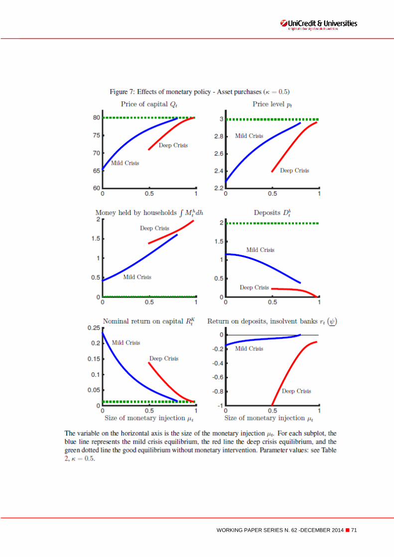
71 WORKING PAPER SERIES N. 62 -DECEMBER 2014 ■

72 WORKING PAPER SERIES N. 62 -DECEMBER 2014 ■

73 WORKING PAPER SERIES N. 62 -DECEMBER 2014 ■

74 WORKING PAPER SERIES N. 62 -DECEMBER 2014 ■

75 WORKING PAPER SERIES N. 62 -DECEMBER 2014 ■

76 WORKING PAPER SERIES N. 62 -DECEMBER 2014 ■
77 WORKING PAPER SERIES N. 62 -DECEMBER 2014 ■
UniCredit & Universities
Knight of Labor Ugo Foscolo Foundation
Piazza Gae Aulenti, UniCredit Tower – Torre A
20154 Milan
Italy
Giannantonio De Roni – Secretary General
Annalisa Aleati - Scientific Director
Sara Colnaghi
Info at:
www.unicreditanduniversities.eu

1