financial constraints and investment: an alternative
TRANSCRIPT

Anales de Estudios Economicos y Empresariales, Vol. XVII, 2007, 9-41 9
Financial Constraints and Investment: An
Alternative Empirical Framework
Sean Cleary1, Bert D’Espallier2
1 Department of Finance, Information Systems, and Management Science, Saint Mary’s
University, Halifax, Canada
2 KIZOK, Research Centre for Entrepreneurship and Innovation, Hasselt University,
Campus Diepenbeek, Belgium
Abstract In the empirical literature on financial constraints, firms are usually
assigned to distinct groups, according to whether or not they are supposed to
be financially constrained (FC). Several recent empirical papers studying the re-
lationship between firms’ cash flows and investment, have found mixed results
regarding whether or not more FC firms show higher or lower sensitivity of invest-
ment to cash flows (CFSI). We show that these mixed results may be attributable
to the use of different “ex-ante” sample-splitting schemes. In response to these is-
sues, we develop a novel research strategy that allows for estimating firm-specific
investment-cash flow sensitivities and identifying the whole distribution of sen-
sitivities across firms. Specifically, we apply entropy-based estimation methods,
which outperform classical estimation methods under various general conditions.
Our empirical results, based on a large panel-data set of U.S. firms, demonstrate
some of the limitations of prevailing classification schemes. The approach we pro-
pose offers new and interesting prospects for re-examining the existing empirical
evidence on financial constraints.
Correspondence to: Bert D’Espallier (e-mail: [email protected])
10 Sean Cleary, Bert D’Espallier
Keywords Corporate finance, investment-cash flow sensitivities, ex-ante sam-
ple splitting, firm heterogeneity, generalized maximum entropy.
JEL Classification G3, G31.
1 Introduction
The impact of capital market frictions on corporate financing policies has been
the focus of a large number of theoretical and empirical studies. Both theory and
empirics highlight the existence of financial constraints (FC) that potentially limit
the capacity of the firm to grow over time. While theoretical arguments, related to
asymmetric information and agency problems, seem compelling and fully in line
with the pecking order corporate finance paradigm (Jensen and Meckling (1977),
Myers and Majluf (1984)), results from the empirical literature are mixed and
are often conflicting, showing a lack of consensus about an adequate and reliable
measure to capture constraints.
The metric most widely believed to be informative about the level of con-
straints, is the cash flow sensitivity of investment (CFSI). This parameter mea-
sures the investment response as a result of an increase in cash flow and was first
proposed in the seminal study by Fazzari et al. (1988). More recent research has
revealed some theoretical inconsistencies as well as conflicting empirical evidence.
On the theoretical side, Kaplan and Zingales (2000) argue that investment-cash
flow sensitivities might not increase monotonically with the level of FC, making
an aggregate sensitivity difficult to interpret. Additionally, Cooper and Ejarque
(2003) and Alti (2003) show that under certain conditions, firms might invest
according to retained earnings, even in the absence of market frictions. On the
empirical side, Kaplan and Zingales (1997), Cleary (1999), and Kadapakkam et
al. (1998) find that investment-cash flow sensitivities may actually be lower for
firms ex-ante identified as being constrained, thereby contradicting most of the
previous empirical evidence. Thus, while the literature recognizes that cash flow
is a significant determinant of corporate investments, it remains unclear to what
Financial Constraints and Investment: An Alternative Empirical Framework 11
extent a significant sensitivity truly reflects the existence of financial constraints
(Pawlina and Renneboog (2005)).
One reason why the CFSI metric is difficult to evaluate lies within its econo-
metrical operationalization. Methodologically, estimation of the CFSI for a cer-
tain sample proceeds along the following line of reasoning: Firstly, the sample
under study is split up in sub-samples according to a criterion that is chosen
to reflect differences in “susceptibility” to capital market imperfections such as
size, payout policy, debt rating, etc. Then, for each sub-sample, an aggregate sen-
sitivity is estimated by regressing corporate investment on operational cash flow
and a number of controls using standard panel data regression techniques. The
“traditional” (i.e., Fazzari et al. (1988)) finding is that the aggregate sensitivity
is higher for the sub-sample most susceptible to capital market imperfections,
which is considered evidence in favour of the CFSI metric. Conversely, the find-
ing that the aggregate sensitivity is lower for the sub-sample most susceptible
to capital market imperfections is considered evidence against the CFSI metric.
This practice, common to all empirical studies in this literature, can be labelled
“ex-ante sample splitting”.
This methodological operationalization is limited and can be misleading be-
cause different splits might produce conflicting estimation results for the sample
under study. In effect, such an inconsistency might reflect two things: (a) the
splitting criterion is unable to distinguish between firms with a different sus-
ceptibility to capital market imperfections (i.e., badly chosen splitting criterion);
and/or, (b) the estimated sensitivity is not indicative of the level of financial con-
straints (i.e., badly chosen metric). The fact that we cannot distinguish between
(a) and (b) makes it very difficult to evaluate the CFSI metric in terms of its
ability to capture financial constraints. Therefore, the results are only as strong
as the choice of the ex-ante sample splitting scheme. Despite the recognition of
this drawback by several authors (Schiantarelli (1995) and Hubbard (1998)), and
despite the limitations of its application, the ex-ante sample splitting remains

12 Sean Cleary, Bert D’Espallier
standard practice even in the most recent literature on investment-cash flow sen-
sitivities (Islam and Mozumdar (2007)), and in the related literature on cash-cash
flow sensitivities (Almeida et al. (2004) and Lin (2007)).
The purpose of this paper is to explore the potential of a new methodolog-
ical operationalization that allows for taking into account firm-specific effects.
We show that the GME estimator developed by Golan et al. (1996) provides
interesting opportunities to model heterogeneous slopes without having to rely
on the assumptions of the classical linear regression model (CLRM). As a result,
firm-specific sensitivities can be estimated making ex-ante sample splitting un-
necessary. Besides the clear benefit of circumventing the ex-ante sample splitting,
the GME estimator has some interesting econometrical properties that make the
estimation results more reliable than traditional GMM estimates (Golan et al.
(1996) and Peeters (2004)).
The remainder of this paper is organized as follows: the next section discusses
existing empirical evidence on financial constraints and on the problems related
to the traditional econometrical operationalization. The third section introduces
the GME estimator and shows how this approach can be applied for estimation
of firm-specific investment-cash flow sensitivities. Section four applies the GME
estimator to a large unbalanced sample of U.S. firms. In section five we conclude
and discuss the benefits and research opportunities this new method provides.
2 Investment-cash flow sensitives and ex-ante sample splitting
The empirical debate on the relationship between financial constraints and firm
investment decisions has been heated. The seminal work of Fazzari et al. (1988)
proposed that investment-cash flow sensitivities are positively related to the ex-
istence of financial constraints. The microeconomic rationale behind this metric
is that financially constrained firms, having only limited access to external funds,
depend mainly on their internally generated funds to finance corporate invest-
ments. As a result, they should display positive investment-cash flow sensitivities,

Financial Constraints and Investment: An Alternative Empirical Framework 13
in contrast with unconstrained firms, who should display no sensitivity to cash
availability. Fazzari et al. (1988) provide empirical evidence supporting their as-
sertion, based on the behaviour of firms exhibiting low payout ratios, which they
argue will be more susceptible to capital market imperfections and, thus, be
more likely to be financially constrained. Many subsequent studies have followed
their approach and have found that investment-cash flow sensitivities are indeed
positively related to the existence of financial constraints, using alternative sam-
ples, investment models or ex-ante sample splitting schemes (Hoshi et al. (1991),
Gilchrist and Himmelberg (1995), Carpenter and Petersen (2002), Bond et al.
(2003), Alayannis and Mozumdar (2004) and Islam and Mozumdar (2007)).
A number of studies have criticized the approach on empirical as well as the-
oretical grounds. Empirical counterexamples have been provided by Kaplan and
Zingales (1997), Kadapakkam et al. (1998) and Cleary (1999), who find that
investment-cash flow sensitivities are lower for firms ex-ante defined as being
constrained. On the theoretical level, some studies have raised questions about
the underlying econometrical design. For example, Bond et al. (2003) suggest
using GMM to account for potential endogeneity of the cash flow parameter,
while Allayannis and Mozumdar (2004) indicate that negative cash flow obser-
vations and influential outliers may have a disproportionately large effect on the
point estimates. Although these studies emphasize a careful econometrical opera-
tionalization of the metric, they do not challenge its usefulness on a fundamental
theoretical level.
Other studies have provided criticism on a more fundamental theoretical
level. Kaplan and Zingales (2007) question the assumed “monotonicity” between
investment-cash flow sensitivities and financial constraints. They also question
the ability of the market-to-book ratio to control for investment opportunities.
Alti (2003) and Cooper and Ejarque (2003) go one step further and show that
under certain conditions, a significant CFSI might occur even in the absence of
capital market imperfections. Finally, Moyen (2004) shows that financially un-

14 Sean Cleary, Bert D’Espallier
constrained firms are inclined to raise more debt in times of high cash flow, which
would be a driving factor for a significant CFSI for unconstrained firms.
While these theoretical considerations cast serious doubt upon the ability of
the CFSI metric to capture financial constraints, it is difficult to assess how strong
this impact is when measuring financial constraints in a “real-world” sample. For
example, Pawlina and Reneboog (2005) and Lin (2007) suggest that the litera-
ture recognizes that investments are driven by internal funds for a large number
of firms, although it remains unclear to what extent these investment-cash flow
sensitivities reflect limited access to external funds as a result of financial con-
straints.
We surmise that the econometric operationalization of “ex-ante sample split-
ting” may contribute to much of the debate in the literature since most previous
studies have split up their sample a priori, using a criterion that is likely to reflect
different susceptibility to capital market imperfections. Popular ex-ante splitting
schemes include: dividend-payout (Fazzari, et al. (1988)); size (Gilchrist and Him-
melberg (1995) and Carpenter and Petersen (2002)); tangibility-ratio (Bhagat et
al. (2005)); debt ratings (Kashyap et al. (1994) and Almeida (2004)); dividend-
investment correlation (Lin (2007)); strength of banking relationships (Hoshi et
al. (1991) and Deloof (1998)); and, cross-country comparison (Kadapakkam et
al. (1998), Bond et al. (2003) and Islam and Mozumdar (2007)). Other studies
have used a statistic that captures a firm’s financial health according to a number
of financial variables (Kaplan and Zingales (1997) and Cleary (1999)).
The main problem with “ex-ante sample splitting” is that an aggregate co-
efficient in a certain sub-sample could be informative about an unobservable
economic phenomenon besides financial constraints. There could be factors re-
lated to the splitting scheme that are not related to financial constraints. To
illustrate this point, consider for instance the commonly used splitting scheme
that uses size as measured by the natural logarithm of total assets. Suppose
the available firm-years are divided into a small group versus a large group, and
Financial Constraints and Investment: An Alternative Empirical Framework 15
the regression analysis reveals a higher aggregate CFSI estimate for the small
sub-sample (as in Gilchrest and Himmelberg (1995), for example). This could
reflect financial constraints, but could equally well reflect another unobservable1
economic phenomenon. For instance, it could reflect that smaller firms invest
mainly in smaller investment projects for which no external capital is required.
In this case, the difference in CFSI reflects a difference in demand for external
funding sources. Alternatively, it could reflect that smaller firms are more active
in industries2 where investments have a shorter time-span but occur more reg-
ularly (i.e. industries that require more capital replacement versus new capital
expenditures). In this case, the difference in CFSI reflects differences in the nature
of the investment projects, rather than financial constraints. Finally, the higher
aggregate CFSI in the smaller sub-sample could simply reflect the presence of
a few influential outliers in the smaller sub-sample that bias the point estimate
upwards.
The conclusion is that estimating an aggregate CFSI can be considered an
indication of financial constraints, but is by no means undisputable empirical
evidence of it. It could be that a researcher is picking up financial constraints,
but it could equally well be that he/she is picking up another unobservable factor
inherent to the splitting criterion. In other words, using ex-ante sample splitting,
a researcher can never be sure whether or not he/she captures constraints. The
results are only as strong as the ex-ante sample splitting criterion is at adequately
reflecting differences in capital market imperfections, which ultimately remains a
matter of assumption (Schiantarelli (1995)). And even if the splitting scheme does
1 Not controlling for unobserved factors is in fact a violation of the “ceteris paribus”principle which might lead to omitted variable bias. Examples of this bias can be foundin standard econometrics textbook such as in Stock and Watson (2007), pg 186-192.
2 Most empirical specifications control for time and industry dummies within eachsub-group, but do not account for industry-differences between the ex-ante definedgroups. Note that using time and industry dummies in each sub-sample separately doesnot solve for differences between the classes.

16 Sean Cleary, Bert D’Espallier
accurately reflect differences in capital market imperfections, the point estimates
might be biased when firm-heterogeneity is ignored.
As Hansen et al. (2004) point out3: “when an economic theory is not a theory
of averages, the econometrical operationalization should account for individual
firm-differences and should not be based on means, which statistically neutralize
firm-differences”. Essentially, financial constraints happen at the firm level, not
at an aggregate level. As such, it seems logical that an econometrical operational-
ization should account for firm differences. Following this line of reasoning, we
explore the possibilities of using the GME estimator in the context of financial
constraints. As we will argue in the next section, this approach allows for firm-
heterogeneity, thereby avoiding some of the pitfalls of using an ex-ante sample
splitting approach.
As an additional benefit, the GME methodology is very much suited to tackle
“ill-posed” or “ill-conditioned” problems, in contrast with the traditional Clas-
sical Linear Regression Model (CLRM) that requires many assumptions about
error terms and unobserved heterogeneity. Based upon some experimental de-
signs, Golan et al. (1996) were able to show that the GME estimator tends to
“outperform” the traditional GMM (2SLS) estimator. Therefore, a second aim
of this paper, besides circumventing ex-ante sample splitting, is to come up with
more reliable estimation results.
3 Heterogeneous slopes using entropy econometrics
3.1 An introduction to GME
The fundamentals that underlie the GME estimation procedure are based upon
the concepts of Information Theory. In this context, Entropy is a measure of
3 The context of Hansen et al. (2004) is a Bayesian operationalization of the ResourceBased View, a predominant paradigm in the strategic management literature. Althoughthis context is very different from the context of capital market imperfections, we believethere are many similarities in terms of econometrical operationalization.

Financial Constraints and Investment: An Alternative Empirical Framework 17
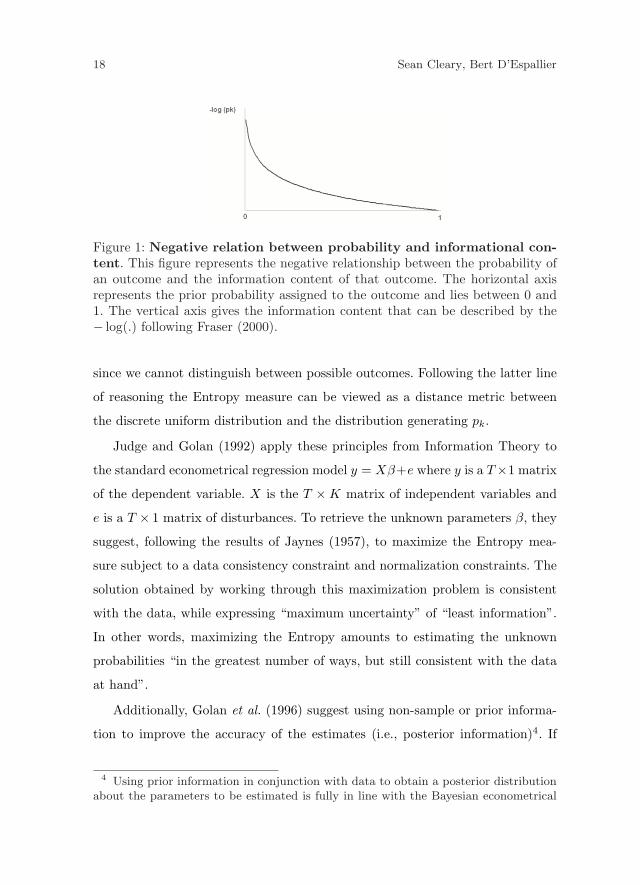
uncertainty or missing information. Let us consider an event X with K discrete
possible outcomes described in a discrete probability distribution (p1, p2, ..., pK).
If an outcome has a small probability of occurring, we would be very surprised
if the outcome did occur, and therefore ascribe a large amount of information
content to that outcome. Vice-versa, for an outcome with a high probability,
occurrence would be anything but surprising and hence occurrence is less in-
formative. Generally the information content of a single outcome is inversely
proportional to its probability and can be written as Ik = − log(pk).
Fraser (2000) provides an intuitive example of the information measure using
the analogy of a cricket match between England and Australia, which we trans-
form to a soccer match between Belgium and the Netherlands. Suppose we define
the soccer match as a Bernoulli trial with success defined as a win for Belgium.
Unfortunately, anyone who has witnessed previous encounters must admit that
success has only a small chance of occurring. Therefore we would be surprised if
Belgium won and this outcome would be very informative about the quality of
Belgian soccer. We would not be surprised if Belgium lost, and the information
content of that outcome provides little information since it was expected with
near certainty. Figure 1 gives a graphical representation of the inverse relation
between probability and uncertainty.
The Entropy or Expected Information of an event is the average information
content of each possible outcome and can be written as:
H(p) = −K∑
k=1
pk ln pk. (1)
The Entropy measure reaches a minimum value of zero when pk = 0, for k =
1, . . . , K. In this case, all possible outcomes have a zero chance of occurring and
missing information is zero. he measure reaches a maximum when p1 = p2 =
... = pK = 1/K. In this special case all outcomes are uniformly distributed and
have an equal chance of occurring. In that case missing information is maximal,
18 Sean Cleary, Bert D’Espallier
Figure 1: Negative relation between probability and informational con-tent. This figure represents the negative relationship between the probability ofan outcome and the information content of that outcome. The horizontal axisrepresents the prior probability assigned to the outcome and lies between 0 and1. The vertical axis gives the information content that can be described by the− log(.) following Fraser (2000).
since we cannot distinguish between possible outcomes. Following the latter line
of reasoning the Entropy measure can be viewed as a distance metric between
the discrete uniform distribution and the distribution generating pk.
Judge and Golan (1992) apply these principles from Information Theory to
the standard econometrical regression model y = Xβ+e where y is a T×1 matrix
of the dependent variable. X is the T ×K matrix of independent variables and
e is a T × 1 matrix of disturbances. To retrieve the unknown parameters β, they
suggest, following the results of Jaynes (1957), to maximize the Entropy mea-
sure subject to a data consistency constraint and normalization constraints. The
solution obtained by working through this maximization problem is consistent
with the data, while expressing “maximum uncertainty” of “least information”.
In other words, maximizing the Entropy amounts to estimating the unknown
probabilities “in the greatest number of ways, but still consistent with the data
at hand”.
Additionally, Golan et al. (1996) suggest using non-sample or prior informa-
tion to improve the accuracy of the estimates (i.e., posterior information)4. If
4 Using prior information in conjunction with data to obtain a posterior distributionabout the parameters to be estimated is fully in line with the Bayesian econometrical
Financial Constraints and Investment: An Alternative Empirical Framework 19
the prior information is fully consistent with the data, zero information is gained
from the data and the posterior distribution will be identical to the prior. When
data do not correspond with prior information, additional information is gained
from the data when calculating the posterior distribution. Since it is necessary for
the support space for β to contain the true value of the parameter, Fraser (2000)
suggests using a discrete support interval around a spike prior with symmetrical
or asymmetrical endpoint depending upon the problem under consideration. The
range should be wide enough to ensure the true value for β to lie within the
interval.
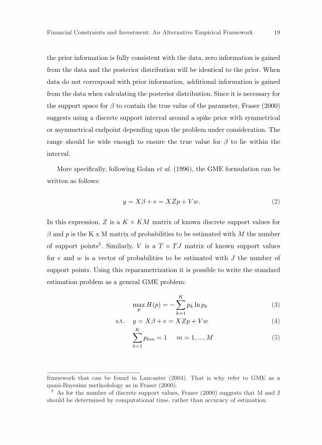
More specifically, following Golan et al. (1996), the GME formulation can be
written as follows:
y = Xβ + e = XZp + V w. (2)
In this expression, Z is a K ×KM matrix of known discrete support values for
β and p is the K x M matrix of probabilities to be estimated with M the number
of support points5. Similarly, V is a T × TJ matrix of known support values
for e and w is a vector of probabilities to be estimated with J the number of
support points. Using this reparametrization it is possible to write the standard
estimation problem as a general GME problem:
maxp
H(p) = −K∑
k=1
pk ln pk (3)
s.t. y = Xβ + e = XZp + V w (4)K∑
k=1
pkm = 1 m = 1, ..., M (5)
framework that can be found in Lancaster (2004). That is why refer to GME as aquasi-Bayesian methodology as in Fraser (2000).
5 As for the number of discrete support values, Fraser (2000) suggests that M and Jshould be determined by computational time, rather than accuracy of estimation.
20 Sean Cleary, Bert D’Espallier
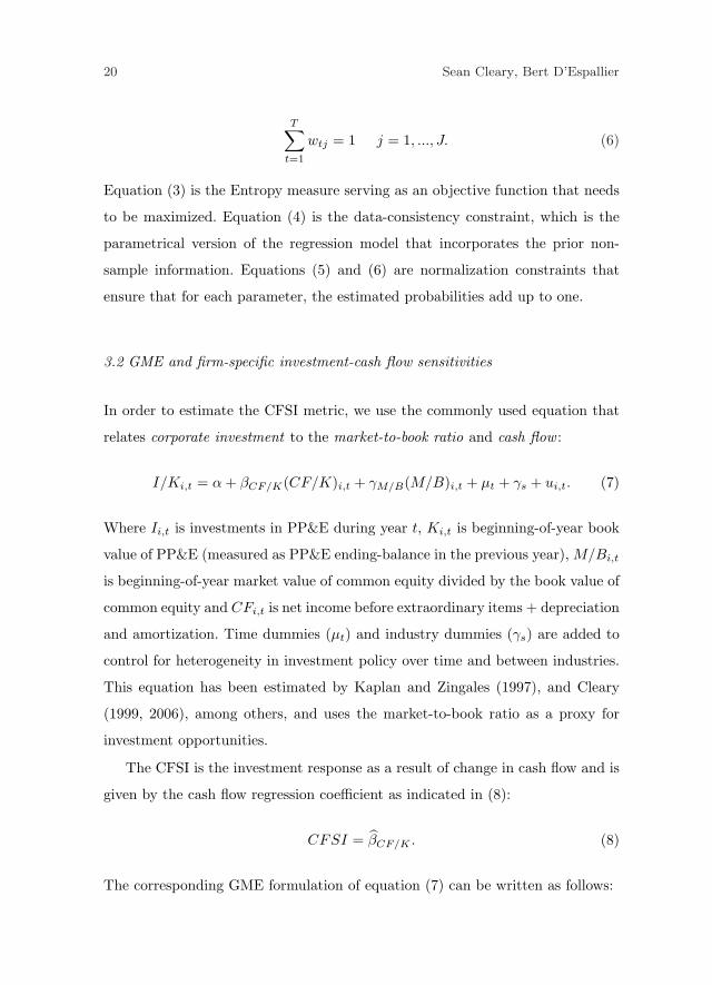
T∑t=1
wtj = 1 j = 1, ..., J. (6)
Equation (3) is the Entropy measure serving as an objective function that needs
to be maximized. Equation (4) is the data-consistency constraint, which is the
parametrical version of the regression model that incorporates the prior non-
sample information. Equations (5) and (6) are normalization constraints that
ensure that for each parameter, the estimated probabilities add up to one.
3.2 GME and firm-specific investment-cash flow sensitivities
In order to estimate the CFSI metric, we use the commonly used equation that
relates corporate investment to the market-to-book ratio and cash flow :
I/Ki,t = α + βCF/K(CF/K)i,t + γM/B(M/B)i,t + µt + γs + ui,t. (7)
Where Ii,t is investments in PP&E during year t, Ki,t is beginning-of-year book
value of PP&E (measured as PP&E ending-balance in the previous year), M/Bi,t
is beginning-of-year market value of common equity divided by the book value of
common equity and CFi,t is net income before extraordinary items + depreciation
and amortization. Time dummies (µt) and industry dummies (γs) are added to
control for heterogeneity in investment policy over time and between industries.
This equation has been estimated by Kaplan and Zingales (1997), and Cleary
(1999, 2006), among others, and uses the market-to-book ratio as a proxy for
investment opportunities.
The CFSI is the investment response as a result of change in cash flow and is
given by the cash flow regression coefficient as indicated in (8):
CFSI = βCF/K . (8)
The corresponding GME formulation of equation (7) can be written as follows:

Financial Constraints and Investment: An Alternative Empirical Framework 21
maxp
H(.) = −∑m
pαm ln pαm −∑m
pβm ln pβm −∑
i
∑m
pνi,m ln pνi,m (9)
−∑m
pγm ln pγm −∑
i
∑m
pµi,mln pµi,m
s.t. I/Ki,t =∑m
pαmsαm +
(∑m
pβmsβm +∑m
pνmsνi,m
)CF/Ki,t (10)
+
(∑m
pγmsγm
)M/Bi,t +
∑m
pµi,msµm
∑m
pαm=
∑m
pβm =∑m
pνi,m=
∑m
pγm=
∑m
pµi,m = 1. (11)
In this formulation equation (9) is the objective function, which is the Entropy-
measure that needs to be maximized with respect to p in order to estimate the
unknown probabilities. Equation (10) is the data-consistency constraint which
is the parametrical version of the CFSI model given in equation (7). In this
equation, each parameter is defined as a linear combination of the predetermined
support vector s and a vector of probabilities p. The support vector s summarizes
the non-sample or prior information in a discrete interval around the spike value
ψ. We model this interval as follows:
sβm = bψβ − 3σβ ; ψβ ; ψβ + 3σβc. (12)
Where ψβ is the spike value for β given by βCF/K , the estimated cash flow
coefficient from running a GMM regression analysis of equation (7). The second
set of constraints in (11) summarizes the normalization constraints, which ensure
that for each parameter, the estimated probabilities sum up to one.
Maximizing equation (9) with respect to p subject to the constraints in (10)
and (11) yields parameter estimates for all unknown parameters; that is:
α =∑m
pαmsαm , β =∑m
pβmsβm , ν =∑m
pνi,msνm , γ =∑m
pγmsνm .
Hence we have model that allows for firm-specific slopes as follows:

22 Sean Cleary, Bert D’Espallier
I/Ki,t = α + (β + νi)CF/Ki,t + γM/B(M/B)i,t + ui,t, (13)
CFSIi = β + νi. (14)
Equation (14) represents the firm-specific investment-cash flow sensitivities esti-
mated with GME as opposed to a single aggregate CFSI estimated in the tra-
ditional regression framework. Hence, it is no longer needed to rely on ex-ante
sample splitting. Instead, we can focus directly on the metric and its ability to
capture constraints. In the discussion section we explore conceptually how these
individual sensitivities can be used to evaluate the metric in its ability to capture
constraints.
Besides the conceptual benefit of circumventing the ex-ante sample splitting
there are two additional econometrical benefits worth mentioning. First, the GME
estimator tackles a number of problems that might bias the estimates of the
CLRM, such as under-determinacy and ill-conditioning. A problem is under-
determined when the number of parameters exceeds the number of data points.
Ill-conditioning occurs when the data are generated non-experimentally or linear
dependencies exist among the set of explanatory variables. Golan et al. (1996)
point out that these problems, which are likely to occur in any practical ap-
plication in economics, could lead to unstable parameter estimates and unreli-
able hypothesis testing. Secondly, econometrical research by Pesaran and Smith
(1995) has shown that pooled regression estimates can be highly misleading when
estimating relationships in heterogeneous panels. In fact, this might be the econo-
metrical rationale behind the finding of Allayannis and Mozumdar (2004) that a
few influential outliers could heavily bias an aggregate CFSI estimate. The GME
estimator does not suffer from this potential bias, because slope heterogeneity
is allowed for. Moreover, studying the distribution of firm-specific sensitivities
could give further insights in the nature of the bias of an aggregate coefficient in
different sub-samples.
Financial Constraints and Investment: An Alternative Empirical Framework 23
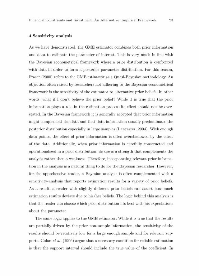
4 Sensitivity analysis
As we have demonstrated, the GME estimator combines both prior information
and data to estimate the parameter of interest. This is very much in line with
the Bayesian econometrical framework where a prior distribution is confronted
with data in order to form a posterior parameter distribution. For this reason,
Fraser (2000) refers to the GME estimator as a Quasi-Bayesian methodology. An
objection often raised by researchers not adhering to the Bayesian econometrical
framework is the sensitivity of the estimator to alternative prior beliefs. In other
words: what if I don’t believe the prior belief? While it is true that the prior
information plays a role in the estimation process its effect should not be over-
stated. In the Bayesian framework it is generally accepted that prior information
might complement the data and that data information usually predominates the
posterior distribution especially in large samples (Lancaster, 2004). With enough
data points, the effect of prior information is often overshadowed by the effect
of the data. Additionally, when prior information is carefully constructed and
operationalized in a prior distribution, its use is a strength that complements the
analysis rather then a weakness. Therefore, incorporating relevant prior informa-
tion in the analysis is a natural thing to do for the Bayesian researcher. However,
for the apprehensive reader, a Bayesian analysis is often complemented with a
sensitivity-analysis that reports estimation results for a variety of prior beliefs.
As a result, a reader with slightly different prior beliefs can assert how much
estimation results deviate due to his/her beliefs. The logic behind this analysis is
that the reader can choose which prior distribution fits best with his expectations
about the parameter.
The same logic applies to the GME estimator. While it is true that the results
are partially driven by the prior non-sample information, the sensitivity of the
results should be relatively low for a large enough sample and for relevant sup-
ports. Golan et al. (1996) argue that a necessary condition for reliable estimation
is that the support interval should include the true value of the coefficient. In
24 Sean Cleary, Bert D’Espallier
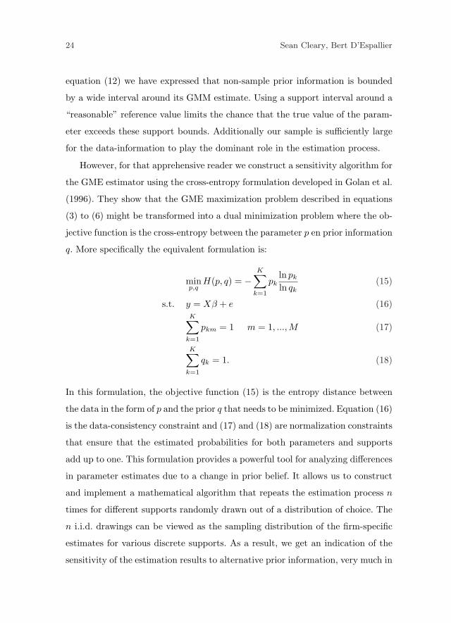
equation (12) we have expressed that non-sample prior information is bounded
by a wide interval around its GMM estimate. Using a support interval around a
“reasonable” reference value limits the chance that the true value of the param-
eter exceeds these support bounds. Additionally our sample is sufficiently large
for the data-information to play the dominant role in the estimation process.
However, for that apprehensive reader we construct a sensitivity algorithm for
the GME estimator using the cross-entropy formulation developed in Golan et al.
(1996). They show that the GME maximization problem described in equations
(3) to (6) might be transformed into a dual minimization problem where the ob-
jective function is the cross-entropy between the parameter p en prior information
q. More specifically the equivalent formulation is:
minp,q
H(p, q) = −K∑
k=1
pkln pk
ln qk(15)
s.t. y = Xβ + e (16)K∑
k=1
pkm = 1 m = 1, ..., M (17)
K∑
k=1
qk = 1. (18)
In this formulation, the objective function (15) is the entropy distance between
the data in the form of p and the prior q that needs to be minimized. Equation (16)
is the data-consistency constraint and (17) and (18) are normalization constraints
that ensure that the estimated probabilities for both parameters and supports
add up to one. This formulation provides a powerful tool for analyzing differences
in parameter estimates due to a change in prior belief. It allows us to construct
and implement a mathematical algorithm that repeats the estimation process n
times for different supports randomly drawn out of a distribution of choice. The
n i.i.d. drawings can be viewed as the sampling distribution of the firm-specific
estimates for various discrete supports. As a result, we get an indication of the
sensitivity of the estimation results to alternative prior information, very much in
Financial Constraints and Investment: An Alternative Empirical Framework 25
line with the sensitivity-analysis that usually complements a Bayesian estimation
problem. The next section includes a table that summarizes a sensitivity-analysis
where the posterior means CFSI is presented for a variety of prior distributions.
5 Results
5.1 Data and summary statistics
Annual data of US-based firms were extracted from the COMPUSTAT database
over the seven year time period from 1998 to 2004. Regulated and Financial
industries according to their two-digit SIC code were deleted (i.e., 43XX, 48XX,
49XX, 6XXX, 9XXX). The only requirement for inclusion in the dataset is that
firms report no negative values for M/B, TA or K during the sample period. In
order to remove outliers, the top and lowest 1% of observations was deleted for
every variable used. As an additional check, all variables required for estimation of
the regression equation (7) were winsorized6 in order to reduce impact of extreme
observations, while keeping as much information in the dataset. These procedures
leave us with a large unbalanced dataset of 25,879 firm-year observations.
Table 1 presents descriptive statistics for a selection of financial variables. The
mean value of total assets is around $2.3 billion. Median sales growth, defined
as the percentage growth of annual sales, is around 8%. The average debt ratio
is about 26% and the mean payout ratio is 12.4%. Mean values for cash flow to
net fixed assets, total capital expenditures to net fixed assets and the market-
to-book ratio are 11.4%, 17.0% and 2.62 respectively. Finally, the averages for
the tangibility-ratio (measured as PP&E divided by net fixed assets), the current
ratio and for ROE (defined as income before extraordinary items divided by
common equity) are 64.1%, 2.8 and 1.2% respectively.
6 The following winsorizing rules were used, as in Cleary (1999): I/Ki,t = 2, ifI/Ki,t > 2; I/Ki,t = −2, if I/Ki;t < −2; MBi,t = 10, if MBi,t > 10; CF/Ki,t = 5, ifCF/Ki,t > 5; CF/Ki,t = −5, if CF/Ki,t < −5.

26 Sean Cleary, Bert D’Espallier
mean Q1 median Q3Total Assets (x $ 1,000) 2,331 42.48 235.33 1164.25Sales growth (%) 3.03% -3.98% 7.99% 23.48%Payout ratio (%) 12.37% 0% 0% 11.20%Debt ratio (%) 26.43% 2.91% 19.90% 36.78%CF/K (%) 11.42% 0.53% 14.11% 33.86%Inv/K (%) 17.01% 5.16% 9.73% 18.64%MB (%) 2.62 0.98 1.78 3.28Slack/K (%) 128.00% 20.04% 65.67% 192%ROE (%) 1.16% -5.54% 7.98% 16.17%Current ratio (%) 2.78 1.19 1.88 3.09PP&E/K (%) 64.12% 22.21% 44.78% 78.02%
Table 1: Descriptive Statistics. This table presents means and Quartiles fora number of financial and growth variables. Payout-ratio is defined as total div-idends and stock repurchases divided by net income. Debt-ratio is total debtdivided by total assets. Slack is defined as (cash holdings + short-term invest-ments + 0.5 inventories + 0.7 accounts receivables – short term loans). Thesample consists of 25,879 observations over a 7 year time-period from 1998-2004.
5.2 Pooled estimation using GMM
Following the traditional econometrical operationalization, equation (7) was es-
timated using GMM7 for various sub-samples split up according to a priori mea-
sures of financing frictions. We experiment with 5 different splitting schemes that
have been used extensively in the literature: payout ratio, size, tangibility ratio,
debt rating and KZ index.
Scheme 1: Payout ratio
Following Fazzari et al. (1988), Almeida et al. (2004) and others, firms were
ranked annually according to their payout ratio, defined as total dividends and
stock repurchases divided by net income. Firms in the bottom (top) three deciles
of the payout distribution were labelled LOW-PAYOUT (HIGH-PAYOUT). The
annual ranking is to ensure that firms are able to change ex-ante constraints
status over the sample period, which makes the sample splitting less rigid, as
pointed out by Schiantarelli (1997).
7 The GMM estimator developed by Arellano and Bond (1991) was used in order tocontrol for potential endogeneity of the cash flow parameter (Bond et al., 2003).

Financial Constraints and Investment: An Alternative Empirical Framework 27
Scheme 2: Size
Following Gilchrest and Himmelberg (1995) and Kadapakkam et al. (1998) among
others, firms were ranked annually according to their size measured as the natural
log of total assets. Firms in the bottom (top) three deciles of this size-distribution
were labelled SMALL (LARGE).
Scheme 3: Tangibility ratio
Following Bhagat et al. (2005), firms were ranked annually according to their
tangibility ratio measured as PP&E divided by net fixed-assets. Again, firms in
the bottom (top) three deciles of the tangibility-distribution were labelled LOW
TANG (HIGH TANG).
Scheme 4: Debt rating
Following Kashyap et al. (1994) among others, firms were labelled RATED if
their debt was rated during that year, and labelled UNRATED if their debt was
not rated. Again, this classification was verified annually in order for firms to
“jump” constraints status during the sample period.
Scheme 5: KZ index
Following Lamont et al. (2001) and Almeida et al. (2004), we construct a linear
index of firm financial constraints that can be written as follows:
KZ = −1.002× CF + 0.283×Q + 3.139× Leverage− 39.368×Dividends
−1.315× Cash holdings.
This index is believed to be positively related to the level of financial constraints
according to a factoring analysis as described in the Kaplan and Zangales (1997)
study. We rank firms annually according to this index and label firms in the
bottom (top) three deciles of the distribution as LOW KZ (HIGH KZ).
28 Sean Cleary, Bert D’Espallier
Table 2 summarizes the number of firm-years for each classification scheme
and the association between the schemes in terms of percentage overlap between
the schemes. For instance, the first column indicates that 8,634 firm-years were
classified as having a LOW PAYOUT-RATIO. Of these 8,634 observations, 38.8%
were labelled SMALL according to the second classification scheme, 34.2% were
labelled LOW TANG according to the third classification scheme, 80.8% were
UNRATED and 32.2% had a HIGH KZ index. As such, this table indicates how
consistently different classification schemes capture observations.
In general, we see that there is a somewhat positive association between the
schemes. However, this positive association is rather low for most of the schemes.
For instance, of the 7,741 firm-years classified as SMALL, 32% had a LOW TANG
RATIO. However, an almost equal share of 27.3% actually received a classification
HIGH TANG RATIO. This means that a substantial share of observations defined
as constrained according to one splitting scheme, received a classification as being
unconstrained according to a second splitting scheme. This is not an exception
as can be seen by going through the table. For instance, of the 9,652 observations
with a HIGH PAYOUT RATIO, 57.5% are labelled UNRATED according to
the debt rating scheme. This means that the majority of observations classified
unconstrained by the first classification scheme, were classified constrained by
the fourth classification scheme.
Generally, the schemes payout, size and debt rating tend to be most positively
correlated, whereas the tangibility ratio and the KZ index produce less clear pos-
itive correlations. But even when the schemes are positively associated, overlaps
between the schemes rarely exceed 50%, which would mean at least half of the
observations would receive the same ex-ante classification according to different
schemes.
We believe that Table 2 indicates a potential problem with the ex-ante sample
splitting framework, namely the inability to capture the same observations. The
schemes are not able to identify undisputably those firms that are more likely

Financial Constraints and Investment: An Alternative Empirical Framework 29
Payoutra
tio
Fir
msi
zeTangib
ility
ratio
Debtra
ting
KZ
index
Low
Hig
hSm
all
Larg
eLow
Hig
hU
nra
ted
Rate
dH
igh
Low
Payout
rati
oLow
8,6
34
Hig
h9,6
52
Fir
msi
ze
Sm
all
38.8
%15.5
%7,7
41
Larg
e18.8
%48.2
%7,7
97
Tangib
ility
rati
oLow
34.2
%21.6
%32.0
%23.0
%7,5
95
Hig
h26.0
%37.1
%27.3
%38.9
%7,8
42
Debt
rati
ng
Unra
ted
80.8
%57.5
%99.8
%25.1
%79.4
%3.0
%18,6
00
Rate
d19.2
%42.5
%0.2
%74.9
%20.6
%54.2
%7,2
79
KZ
Index
Hig
h32.2
%21.9
%27.5
%22.3
%7.9
%54.3
%32.1
%37.3
%7,3
19
Low
27.0
%30.7
%32.1
%31.5
%68.1
%3.0
%28.8
%18.6
%7,3
36
Tab
le2:
Ass
oci
atio
nac
ross
ex-a
nte
splitt
ing
schem
es.
Thi
sta
ble
pres
ents
num
ber
offir
m-y
ears
and
asso
ciat
ion
acro
ssth
edi
ffere
ntex
-ant
esa
mpl
esp
litti
ngsc
hem
es.T
hedi
agon
alel
emen
tsre
pres
ent
the
num
ber
offir
m-y
ears
wit
hin
each
sub-
sam
ple
ofth
eva
riou
ssp
litti
ngsc
hem
es.T
his
num
ber
offir
m-y
ears
isfu
rthe
rsp
litup
inth
eva
riou
ssp
litti
ngsc
hem
esin
the
off-d
iago
nalel
emen
ts.
30 Sean Cleary, Bert D’Espallier
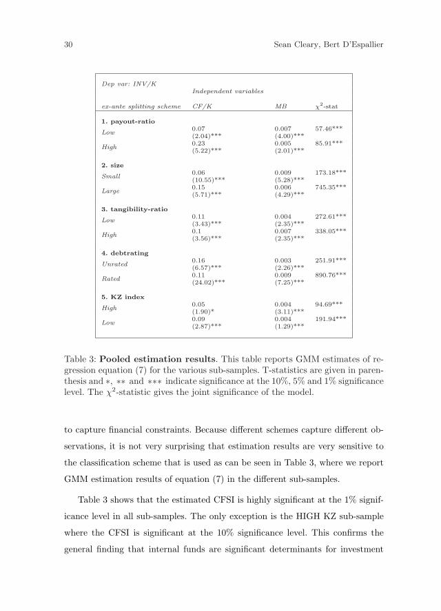
Dep var: INV/KIndependent variables
ex-ante splitting scheme CF/K MB χ2-stat
1. payout-ratio
Low0.07 0.007 57.46***(2.04)*** (4.00)***
High0.23 0.005 85.91***(5.22)*** (2.01)***
2. size
Small0.06 0.009 173.18***(10.55)*** (5.28)***
Large0.15 0.006 745.35***(5.71)*** (4.29)***
3. tangibility-ratio
Low0.11 0.004 272.61***(3.43)*** (2.35)***
High0.1 0.007 338.05***(3.56)*** (2.35)***
4. debtrating
Unrated0.16 0.003 251.91***(6.57)*** (2.26)***
Rated0.11 0.009 890.76***(24.02)*** (7.25)***
5. KZ index
High0.05 0.004 94.69***(1.90)* (3.11)***
Low0.09 0.004 191.94***(2.87)*** (1.29)***
Table 3: Pooled estimation results. This table reports GMM estimates of re-gression equation (7) for the various sub-samples. T-statistics are given in paren-thesis and ∗, ∗∗ and ∗∗∗ indicate significance at the 10%, 5% and 1% significancelevel. The χ2-statistic gives the joint significance of the model.
to capture financial constraints. Because different schemes capture different ob-
servations, it is not very surprising that estimation results are very sensitive to
the classification scheme that is used as can be seen in Table 3, where we report
GMM estimation results of equation (7) in the different sub-samples.
Table 3 shows that the estimated CFSI is highly significant at the 1% signif-
icance level in all sub-samples. The only exception is the HIGH KZ sub-sample
where the CFSI is significant at the 10% significance level. This confirms the
general finding that internal funds are significant determinants for investment
Financial Constraints and Investment: An Alternative Empirical Framework 31
outlays for most firms. However, in terms of magnitude, the CFSI estimates
differ largely across different splitting schemes. For three classification schemes
(payout, size, KZ index), a higher CFSI is found in the unconstrained sub-sample.
HIGH PAYOUT, LARGE and LOW KZ observations have an estimated sensi-
tivity of 0.23, 0.15 and 0.09 respectively. Their constrained counterparts (LOW
PAYOUT, SMALL, and HIGH KZ) have a lower CFSI with values 0.07, 0.06
and 0.05, respectively. These results support the Kaplan and Zingales (1997),
Cleary (1999), and Kapadakkam (1998) results, in the sense that ex-ante defined
constrained firms exhibit lower investment-cash flow sensitivities.
However, using the debt rating and the tangibility scheme, we find opposite
results. The LOW TANGIBILITY and UNRATED observations have a higher
estimated CFSI with values 0.11 and 0.16, respectively. These results are in line
with Fazzari et al. (1988), Carpenter and Petersen (2002), among others who
find that investment-cash flow sensitivities are higher in firms ex-ante defined as
being constrained. As we have argued before, all this is not very surprising given
the low overlap between the different schemes.
5.3 Firm-heterogeneity using GME
In Table 4 we report the firm-specific sensitivities estimated by the GME proce-
dure described in equations (9)- (13). The mean sensitivity is 0.19, which comes
from a wide variation in firm-specific estimates ranging from a minimum of -0.3
to a maximum of 1.3. These are consistent with estimates for the full samples
provided by previous studies. Some 13% of the firms show a negative sensitivity
over the observed sample period, which means positive investments despite nega-
tive cash flows, or vice versa, negative investments (divestitures) despite positive
cash flows. The kernel density graph indicates that the vast majority of the firms
have a positive CFSI with a peak around 0.20. However, closer inspection reveals
that there is also a small bump in the density function around 0.6 indicating
some firms have much higher CFSI estimates.

32 Sean Cleary, Bert D’Espallier
CFSImean 0.19median 0.18minimum -0.3maximum 1.3deciles 10 -0.14
20 -0.0130 0.0740 0.1450 0.1960 0.2370 0.2880 0.3690 0.49
Table 4: GME estimation results. This table reports mean, median, minimum,maximum and deciles of the distribution of firm-specific CFSI estimates estimatedwith the GME estimator described in equations (9)- (13). The table includesthe graph of the kernel density function of the estimated distribution. In thisgraph, the vertical axis represents the percentage of firms and the horizontal axisrepresents the CFSI.
We have identified that an additional benefit of GME is its potential in dealing
with ill-conditioned and ill-posed inference problems. As a result, GME would
produce more accurate and consistent estimation results by reducing the potential
bias from violation of traditional CLRM assumptions. Figure 2 contrasts the
traditional GMM point estimator with the GME distribution for the different
sub-samples resulting from the different ex-ante sample splitting schemes. This
gives us insight into the nature of the bias of an aggregate GMM estimate.
In general, the GMM estimator seems to be influenced to a certain extent
by the observations in the tails of the distribution. For example, the kernel dis-
tribution of high-payout firms is skewed to the right, indicating a small number
of firm-years with rather high investment-cash flow sensitivities. As a result, the
GMM estimate (0.23) lies very much at the right-hand side of the kernel den-
sity. This finding is observable in most sub-samples and is most noticeable in
the last graph of Figure 2 (KZ index). As can be seen, the GME distribution
of high KZ-observations lies further to the right then the distribution of low
KZ-observations. However, the GMM estimate for high KZ-observations (0.05)
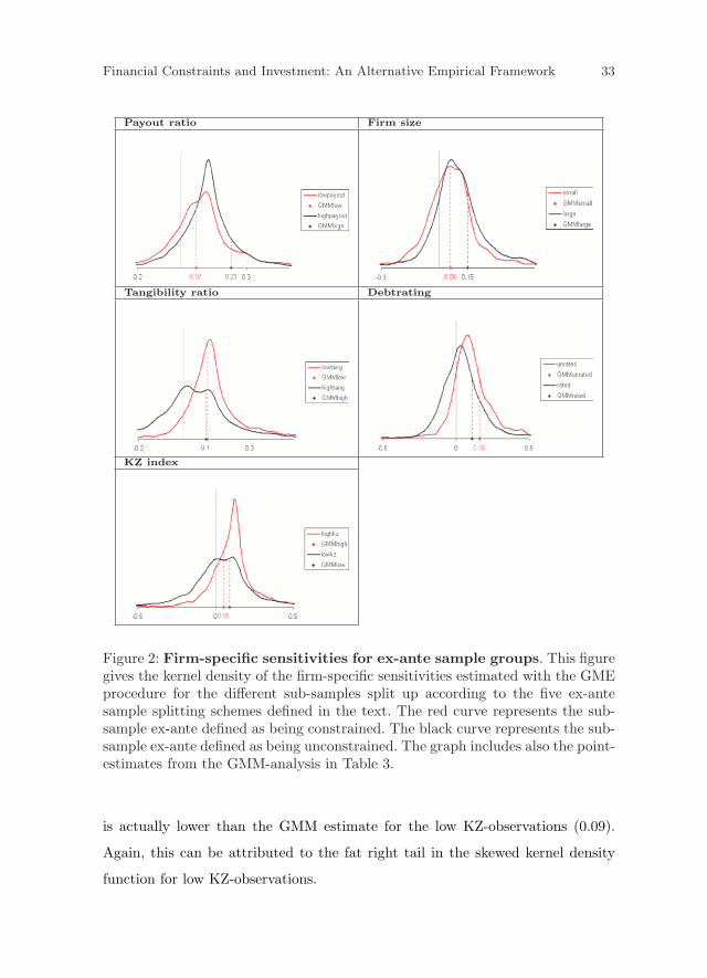
Financial Constraints and Investment: An Alternative Empirical Framework 33
Payout ratio Firm size
Tangibility ratio Debtrating
KZ index
Figure 2: Firm-specific sensitivities for ex-ante sample groups. This figuregives the kernel density of the firm-specific sensitivities estimated with the GMEprocedure for the different sub-samples split up according to the five ex-antesample splitting schemes defined in the text. The red curve represents the sub-sample ex-ante defined as being constrained. The black curve represents the sub-sample ex-ante defined as being unconstrained. The graph includes also the point-estimates from the GMM-analysis in Table 3.
is actually lower than the GMM estimate for the low KZ-observations (0.09).
Again, this can be attributed to the fat right tail in the skewed kernel density
function for low KZ-observations.

34 Sean Cleary, Bert D’Espallier
These findings suggest that a few extreme observations might have a dis-
proportionately large effect on an aggregate sensitivity, which is consistent with
the findings of Allayannis and Mozumdar (2004). The econometrical rationale
behind this finding has been reported by Pesaran and Smith (1994) who argue
that pooled regression estimates can be highly misleading when estimating rela-
tionships in heterogeneous panels. The GME estimator does not suffer from this
potential bias, because slope heterogeneity is allowed for.
5.4 Sensitivity to alternative priors
In the previous section, we described a GCE algorithm for investigating the re-
sponsiveness of the estimation results to the use of alternative prior information.
The idea behind the algorithm is to estimate a posterior mean sensitivity for n
different support values drawn i.i.d. from a prior distribution of choice. Table 5
presents the posterior mean for n = 100 draws from two uniform and a normal
prior distribution. The uniform prior distribution U (-10,10) represents an uni-
formed researcher who has no prior knowledge of the CFSI parameter. The uni-
form prior U (-1,1) represents an equally uninformed researcher, although he/she
has a better clue about the range of the CFSI parameter. The normal prior N
(0.5, 0.3) represents an informed researcher who expects the CFSI parameter to
lie somewhere around 0.5 with a reasonable standard deviation.
Table 5 shows that the mean estimated CFSI is not sensitive to the use of
alternative information. The sensitivity averaged over the different draws is 0.21,
0.21 and 0.19 for the U (-10,10), U (-3,3) and N (0.5,0.3) distribution respectively.
Additionally, for each prior distribution, the standard deviation of the mean
sensitivities is very low (0.0001), indicating a very small variance over the 100
draws. This means that even if we start from very uninformative prior beliefs,
the estimation results will not differ much. In other words, no matter from which
prior information a researcher starts,he/she will reach similar conclusions using
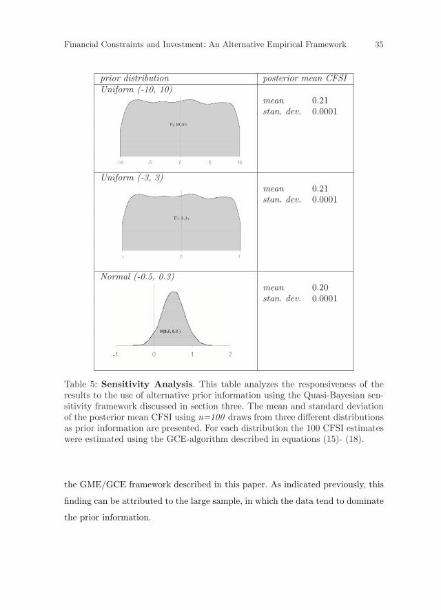
Financial Constraints and Investment: An Alternative Empirical Framework 35
prior distribution posterior mean CFSIUniform (-10, 10)
mean 0.21stan. dev. 0.0001
Uniform (-3, 3)
mean 0.21stan. dev. 0.0001
Normal (-0.5, 0.3)
mean 0.20stan. dev. 0.0001
Table 5: Sensitivity Analysis. This table analyzes the responsiveness of theresults to the use of alternative prior information using the Quasi-Bayesian sen-sitivity framework discussed in section three. The mean and standard deviationof the posterior mean CFSI using n=100 draws from three different distributionsas prior information are presented. For each distribution the 100 CFSI estimateswere estimated using the GCE-algorithm described in equations (15)- (18).
the GME/GCE framework described in this paper. As indicated previously, this
finding can be attributed to the large sample, in which the data tend to dominate
the prior information.

36 Sean Cleary, Bert D’Espallier
6 Conclusions and discussions
This paper uses recent advances in econometrics to address a key problem in
the empirical literature on financial constraints. All existing studies compare ag-
gregate investment-cash flow sensitivities between ex-ante defined sub-samples
using standard regression techniques. Such an ex-ante sample splitting frame-
work, however, comes with a number of limitations. Firstly, the results are only
as strong as the splitting scheme used to reflect different degrees in capital market
imperfections, which is subjective in nature. We have demonstrated that some
“popular” splitting schemes do not necessarily capture the same firm-year ob-
servations and classification overlaps across various schemes are rather low. As
a result, the estimates are sensitive to the splitting scheme that is used. Using
five schemes that have been used extensively in the literature, we find that two
schemes reflect the view of Fazzari et al. (1988), and three schemes contradict
this view. Secondly, a point estimate in a certain sub-sample summarizes all
available firm-year information of that sub-sample into a single aggregate coeffi-
cient, thereby ignoring firm heterogeneity. As a result, much relevant firm-specific
information is ignored and statistically neutralized (Hansen, 2004). Finally, an
aggregate coefficient might be influenced heavily by a few influential outliers as
indicated by Allayannis and Mozumdar (2004) and Pesaran and Smith (1995).
These limitations pose difficulties for the traditional econometrical opera-
tionalization of estimating regressions in ex-ante defined sub-samples. Our ap-
proach allows for firm-specific sensitivities by introducing slope heterogeneity
into the regression equation. Consequently, ex-ante sample splitting is no longer
necessary, and the usefulness of the CFSI metric can be evaluated directly. We
show that the GME estimator developed by Golan et al. (1996) is very much
suited for introducing slope heterogeneity. We show the calculations for a large
unbalanced sample of US listed firms and find a wide sensitivity ranging from
-0.3 through 1.3.
Financial Constraints and Investment: An Alternative Empirical Framework 37
Moreover, allowing for firm differences enables us to study the entire distri-
bution of firm-specific sensitivities, which provides insights into the nature of the
bias of an aggregate point estimate. We find that GMM point estimates tend to
be biased substantially by a few influential outliers. An additional benefit of the
GME estimator is that it does not require any assumptions of the error term
as the CLRM does. As a result, the estimation results should be more accu-
rate and reliable because there is no bias resulting from violations of traditional
assumptions.
It is not our aim in this paper to enter the debate on the relationship between
investment-cash flow sensitivities and financial constraints. Rather, our focus is
on the development of an econometrical operationalization that makes ex-ante
sample splitting unnecessary by taking into account firm-differences. In light of
this, we believe the GME estimator is an exiting new methodology that provides
a number of interesting research opportunities to re-examine the evidence on
financial constraints.
Firstly, as we have indicated before, the firm-specific sensitivities could be
used to make a direct evaluation of the CFSI metric in capturing financial con-
straints. This could be done by isolating different sensitivity classes and com-
paring these classes in terms of financial variables that would be informative
about financial constraints. Building up profiles of different sensitivity classes
would provide valuable insights in the ability if the CFSI metric to capture fi-
nancial constraints. This could be considered an “ex-post” evaluation of financial
constraints in contrast with the ex-ante sample splitting approach.
Secondly, such an evaluative framework of financial constraints could be es-
tablished for alternative metrics of financial constraints as well. Recent research
has witnessed a shift in focus towards an alternative metric, namely the cash
flow sensitivity of cash, believed to be positively related to financial constraints
(Almeida et al. (2004); Khurana et al. (2006); Han and Qiu (2007); Lin (2007)).
Like the CFSI, this metric is also estimated through regression analysis in distinct

38 Sean Cleary, Bert D’Espallier
ex-ante defined sub-samples, and therefore the objections raised in this paper ap-
ply equally well to the literature on cash-cash flow sensitivities. Future research
could aim at evaluating both metrics in their ability to capture financial con-
straints and clear out which metric would be more suitable in different samples
(metric selection).
Finally, in this literature, models differ in several dimensions such as the
time-variation aspect (static versus dynamic models); investment paradigm (Q
models versus neoclassical models versus accelerator models); dependent variable
(investments in fixed assets versus total growth versus R&D assets) and differ-
ent controls for the investment opportunities bias. These different dimensions
yield many possible combinations for model building and results may be sensi-
tive to the specification used. The literature should come to terms as to which
model is best suited to measure constraints for certain populations, by objec-
tively evaluating different models in their ability to capture financial constraints.
Our approach of estimating firm-specific sensitivities and evaluating models on
their discriminating power between ex post defined sensitivity classes provides
interesting research opportunities in this area (model selection).
References
1. Allayannis, G., Mozumdar, A. (2004): The impact of negative cash flow and influen-
tial observations on investment-cash flow sensitivity estimates. Journal of Banking
and Finance, 28 (5), pp. 901-930.
2. Almeida, H., Campello, M., Weisbach, M.S. (2004): The cash flow sensitivity of
cash. Journal of Finance, 59 (4), pp. 1777-1804.
3. Alti, A. (2003): How sensitive is investment to cash flow when financing is friction-
less? Journal of Finance, 58 (2), pp. 707-722.
4. Arellano, M., Bond, S.R. (1991): Some tests of specification for panel data: Monte
Carlo Evidence and an Application to Employment Equations. The Review of Eco-
nomic Studies, 58, pp. 277-297.

Financial Constraints and Investment: An Alternative Empirical Framework 39
5. Bhagat, S., Moyen, N., Suh, I. (2005): Investment and internal funds of distressed
firms. Journal of Corporate Finance, 11 (3), pp. 449-472.
6. Bond, S., Elston, J.A. , Mairesse, J., Mulkay, B. (2003): Financial factors and
investment in Belgium, France, Germany, and the United Kingdom: a comparison
using company panel data. The Review of Economics and Statistics, 85 (1), pp.
153-165.
7. Carpenter, R.E., Petersen, B.C. (2002): Is the growth of small firms constrained by
internal finance? The Review of Economics and Statistics, 84 (2), pp. 298-309.
8. Cleary, S. (1999): The relationship between firm investment and financial status.
Journal of Finance, 54 (2), pp. 673-691.
9. Cleary, S. (2006): International corporate investment and the relationships between
financial constraints measures. Journal of Banking and Finance, 30, pp. 1559-1580.
10. Cleary, S., Povel, P., Raith, M. (2007): The U-shaped investment curve: theory and
evidence. Journal of Financial and Quantitative Analysis, 42 (1), pp. 1-40.
11. Cooper, R., Ejarque, J. (2003): Financial frictions and investment: Requiem in Q.
Review of Economic Dynamics, 6 (4), pp. 710-728.
12. Deloof, M. (1998): Internal capital markets, bank borrowing, and financial con-
straints: evidence from Belgian firms. Journal of Business Finance and Accounting,
25, pp. 945-968.
13. Fazzari, S.M., Hubbard, R.G., Petersen, B.C. (1988): Financing constraints and
corporate investment. Brookings paper on economic activity, 1, pp. 141-195.
14. Fraser, I. (2000): An application of maximum entropy estimation: the demand for
meat in the United Kingdom. Applied Economics, 32, pp. 45-59.
15. Gilchrist, S., Himmelberg, C.P. (1995): Evidence on the role of cash flow for invest-
ment. Journal of Monetary Economics, 36, pp. 541-572.
16. Golan, A., Judge, G.G., Miller, D. (1996): Maximum Entropy Econometrics: Robust
Estimation with Limited Data. Indianapolis: John Wiley & Sons, Ltd.
17. Hansen, M. H., Perry, L.T., Reese, C.S. (2004): A Bayesian operationalization of
the Resource-Based view. Strategic Management Journal, 25, pp. 1279-1295.
18. Han, S., Qiu, J. (2007): Corporate precautionary cash holdings. Journal of Corpo-
rate Finance, 13 (1), pp. 43-57.

40 Sean Cleary, Bert D’Espallier
19. Hubbard, R.G. (1998): Capital-Market Imperfections and Investment. Journal of
Economic Literature, XXXVI, pp. 193-225.
20. Hoshi, T., Kashyap, A., Scharfstein, D. (1991): Corporate structure, liquidity and
investment: evidence from Japanese industrial groups. Quarterly Journal of Busi-
ness and Finance, 106, pp. 33-60.
21. Islam, S.S., Mozumdar, A. (2007): Financial market development and the impor-
tance of internal cash: Evidence from international data. Journal of Banking and
Finance, 31, pp. 641-658.
22. Jaynes, E. T. (1957): Information theory and statistical mechanics. Physics Review,
106, pp. 620-630.
23. Jensen, M., Meckling, W. (1976): Theory of the firm: managerial behaviour, agency
costs, and ownership structure. Journal of Financial Economics, 3 (4), pp. 305-360.
24. Judge, G.G., Golan, A. (1992): Recovering information in the case of ill-posed in-
verse problems with noise. Working Paper (Department of Agricultural and Natural
Resources, University of California, Berkely, CA).
25. Kadapakkam, P.R., Kumar, P.C., Riddick, L.A. (1998): The impact of cash flows
and firm size on investment: The international evidence. Journal of Banking and
Finance, 22, pp. 293-320.
26. Kaplan, S.N., Zingales, L. (1997): Do investment cash flow sensitivities provide
useful measures of financing constraints? Quarterly Journal of Economics, 112 (1),
pp. 169-215.
27. Kaplan, S.N., Zingales, L. (2000): Investment-cash flow sensitivities are not valid
measures of financing constraints. Quarterly Journal of Economics, 115 (2), pp.
707-712.
28. Kashyap, A., Lamont, O., Stein, J. (1994): Credit conditions and the cyclical be-
havior of inventories. Quarterly Joural of Economics, 109, pp. 565-592.
29. Khurana, I.K., Martin, X., Pereira, R. (2006): Financial development and the cash
flow sensitivity of cash. Journal of Financial and Quantitative Analysis, 41 (4), pp.
787-806.
30. Lamont, O., Polk, C., Saa-Requejo, J. (2001): Financial constraints and stock re-
turns. Review of Financial Studies, 14, pp. 529-554.
Financial Constraints and Investment: An Alternative Empirical Framework 41
31. Lancaster, T. (2004): An introduction to modern Bayesian Econometrics (Malden
USA: Blackwell Publishing).
32. Lin, Y.C (2007): The cash flow sensitivity of cash: evidence from Taiwan. Applied
Financial Economics, 17, pp. 1013-1024.
33. Moyen, N. (2004): Investment-cash flow sensitivities: constrained versus uncon-
strained firms. Journal of Finance, 59, pp. 2061-2092.
34. Myers, S., Majluf, N. (1984): Corporate financing and investment decisions when
firms have information that investors do not have. Journal of Financial Economics,
13 (2), pp. 187-221.
35. Pawlina, G., Renneboog, L. (2005): Is investment cash flow sensitivity caused by the
agency costs or asymmetric information? Evidence from the UK. Working Paper
(ECGI Working Paper Series in Finance, No. 69).
36. Peeters, L. (2004): Estimating a random-coefficients sample-selection model using
generalized maximum entropy. Economics Letters, 84, pp. 87-92.
37. Pesaran, M.H., Smith, R. (1995): Estimating long-run relationships from dynamic
heterogeneous panels. Journal of Econometrics, 68, pp. 79-113.
38. Schiantarelli F. (1995): Financial constraints and investment: a critical review of
methodological issues and international evidence. Working Paper (Boston College
Working Papers in Economics, Vol. 293).
39. Stock, J., Watson, M. (2007): Introduction to Econometrics. Pearson International
Edition, Addison Wesley.