financial analysts accuracy do valuation methods matter

Financial Analysts’ Accuracy: Do valuation methods matter?

(Elisa Cavezzali, Ugo Rigoni1)

Abstract

This study investigates how different ways to evaluate a company influence the accuracy of the target price. We know that finance theory and professional practice propose alternative approaches to the evaluation of a company. The literature on the relationship between the valuation methods used and target price accuracy is still scant, and the results are inconclusive and contradictory.

Coding the valuation methods of 1,650 reports, we find that the accuracy of target prices decreases when the target price is based just on a main method. Furthermore, we show that methods based on company fundamentals and those based on market multiples lead to similar levels of accuracy. Among different classes of methods, there are no superior methods. Therefore, we argue that in order to improve forecast accuracy, analysts need to assess company value by choosing and applying a set of different methods, combining them and getting the average value, but regardless of the specific technique chosen.

Keywords: forecast accuracy, sell-side analysts, equity valuation, valuation methods

1Elisa Cavezzali is Assistant Professor of Corporate Finance at Ca’ Foscari University of Venice, Department of Management, San Giobbe 873, 30121 – Venice, Italy (tel: +39(0)41 2346931, email: [email protected]); Ugo Rigoni is Associate Professor of Financial Markets and Institutions at Ca’ Foscari University of Venice, Department of Management, San Giobbe 873, 30121 – Venice, Italy (tel: +39(0)41 2348770, email: [email protected]). The corresponding author is Elisa Cavezzali: [email protected]

1. Introduction

In this paper we examine how different ways to evaluate a company influence the accuracy of

the valuation output, the target price. Our aim is to investigate the task of valuation by sell-side

analysts by examining the valuation methods actually used and testing whether different methods

have different impacts on the accuracy of the target price.

We know that finance theory and professional practice propose alternative approaches to the

evaluation of a company. The traditional distinction is between valuation methods based on the

fundamentals of the company (future cash flows, earnings and so on) and the market ratios

approach, which is based on the company’s market multiples. Furthermore, within each class of

method, there are different ways to apply it. Analysts also frequently use some low-cost

simplifications of the traditional methods, leading to quick and less accurate value estimates than

would have been arrived at with the full implementation of the original models. There are,

therefore, a variety of methods for company valuation used by practitioners. Different methods

may be applied at the same time in the same report in order to arrive at a target price which is the

average result of the various estimation techniques used, while in other cases, the target price is

the result of the application of just one method, sometimes checked with other control methods.

We try to detect whether different choices of valuation process and technique bring the same

final result and this is measured in terms of the accuracy of the target prices.

Through hand coding the valuation content of a sample of 1,650 reports, issued by 53 different

international investment brokerage houses and covering a total of 48 companies across 20

different sectors, we find that the accuracy of target prices decreases when the target price is

based solely on a main method. Thus, we argue that the analysts can obtain better accuracy

performance by simply combining a few selected techniques, instead of using just one method to

evaluate a company. Furthermore, we show that methods based on company fundamentals and

those based on market multiples lead to similar levels of accuracy. Among the different classes

of evaluation method, there are no superior methods in terms of output performance, the one

standout being the net asset method as it gives a visibly poorer accuracy level. This latter

evidence is consistent with those theories arguing that this method is ‘inferior’ since it is static

and does not capture future opportunities and the different levels of risk of the evaluated

company.

Therefore, in summary, we argue that in order to improve forecast accuracy, analysts need to

assess company value by choosing and applying a set of different methods, combining them and

getting the average value, but regardless of the specific technique chosen.

This paper is mainly related to the literature on target prices and the determinants of their

accuracy, providing new empirical evidence. Prior literature has shown that analysts differ in

their ability to forecast. However, the empirical research has focused mainly on market reaction

to analysts’ earnings, recommendations and revisions. Analysis of the accuracy of target prices

and the relevance of valuation models in the valuation process are relatively unexplored areas of

accounting and finance research. Only a small number of studies have focused on the

relationship between the valuation methods used by sell-side analysts in their reports and target

price accuracy (e.g. Demirakos et al. (2004), Demirakos (2009) and Asquith et al. (2005)), and

the results are still inconclusive and contradictory.

By looking at an extended sample of international analysts’ reports covering European

companies, this study assesses the performance of different company valuation methodologies

and helps to fill a gap in the literature by proposing a new approach for analysing and classifying

the valuation methods used in financial analysts’ reports.

The importance of equity research is well known. Brokerage houses and investment banks issue

thousands of reports on a yearly basis, providing trading advice to investors and forecasts

concerning the future market price of listed stocks. The figures on equity research spending are

impressive. Johnson (2006) showed that equity research by investment banks has reached over

US $20 billion in 2006. Furthermore, both The Wall Street Journal and the Institutional Investor

(II) annually award an ‘oscar’ to the best financial analyst on the basis of the performance of the

reports issued.

Accuracy is, therefore, the key feature of the output of equity research. However, since the

reports are not freely available, studies analysing how the valuation methods used influence the

target price accuracy are rare. Consequently, this study may help fill an important gap in the

literature.

The paper is organised as follows: Section 2 discusses the main results obtained by prior

literature; Section 3 describes the theoretical framework; Section 4 reports the data and data

classification criteria; Section 5 presents the research design; Sections 6 and 7 report the

empirical results, their discussion and interpretation; and Section 8 concludes the paper.

2. Literature review

Sell-side analysts issue reports about the equity valuation of companies. The more verifiable

elements of these reports are earnings forecasts, stock recommendations and target prices.

Earlier studies have mainly focused on the market reaction to analysts’ earnings,

recommendations and revisions. Despite the empirical evidence which shows the relevance of

target prices to the market (see, for instance, Asquith et al. (2005) or Brav and Lehavy (2003)),

the research on the accuracy of target prices is still scant and inconclusive. This paper is mainly

related to the literature on target prices and the determinants of their accuracy, providing new

empirical evidence.

A possible reason for the poor attention given to the target price is that earnings forecasts,

recommendations and target price revisions convey homogeneous information to investors,

leading to the same market reaction. However, Francis and Soffer (1997), Brav and Lehavy

(2003) and Asquith et al. (2005) do not confirm this evidence. They report that target prices

convey new information to the market, independent from recommendations and earnings

forecasts. For instance, Brav and Leavy (2003) show market reaction to target prices which is

both unconditional and conditional on stock recommendations and earning forecast revisions.

Similarly, Asquith et al. (2005) demonstrate that the market reacts to target price revisions

regardless of earnings forecasts revisions. Furthermore, target price revisions cause a market

reaction which is greater than that determined by an equivalent revision in the earnings forecast.

Since target prices are relevant for the market, part of the academic interest in them has focused

on the drivers of their accuracy. The empirical evidence shows a certain variability in target price

accuracy. For instance, Asquith et al. (2005) and Bradshaw and Brown (2006) report a good

level of target price accuracy over a time horizon of 12 months (in at least 50% of cases the

target prices are then reached by the market stock prices are, while De Vincentiis (2010) shows a

poor level of accuracy (above the 30% of cases are successful). There are multiple factors which

have the potential to affect this variability and the empirical results are controversial.

Part of the literature has focused on the features of forecasts, such as the well-documented bias in

estimates and the level of analysts’ optimism. The main empirical results show that forecasts

which are highly inflated with respect to the current market price are more difficult to achieve

(Asquith et al. (2005), Bradshaw and Brown (2006), Bonini et al. (2009), Demirakos et al.

(2009) and De Vincentiis (2010)).

Another part of the literature has focused on firm, stock and analyst characteristics which affect

target price accuracy. Specifically, company size, loss-making firms and company coverage are

positively associated with target accuracy, while stock momentum is negatively related (Bonini

et al. (2009) and De Vincentis (2010)).

Finally, only a few studies have analysed how the tools used by analysts to reach the target price,

i.e. the valuation models, can affect the accuracy of the forecast.

Financial analysts can adopt several different valuation methods to evaluate companies, which

are usually categorised into two different macro-classes: single-period valuation methods, i.e.

market multiples, and multi-period valuation methods, such as discounted cash flow (DCF) and

residual income methods (RIM). Empirical research has shown that financial analysts prefer

single-period earnings models, such as market multiples (Barker (1999), Block (1999), Bradshaw

(2002), Demirakos et al. (2004) and Asquith et al. (2005)) as they are simple to apply. Analysts

adopt more complex and time-consuming multi-period models to value companies which are

characterised by high level of uncertainty due to their highly volatile earnings or unstable growth

(Demirakos et al., 2004). Imam et al. (2008) reported that sell-side analysts increased their

preference for DCF models only in recent years, probably influenced by their clients and their

valuation preferences.

Corporate finance theory and the main financial analysis textbooks suggest estimating a

company’s value using, whenever possible, multi-period valuation methods, the reason being

that they should better capture its fair value (Penman (2003) and Koller et al. (2005)). Using

‘superior’ valuation methods should, therefore, lead to more accurate target prices. This theory is

only partially confirmed in practice. Bradshaw (2004) shows that the analysts who issue more

accurate earnings forecasts and who employ rigorous valuation methods such as RIM get better

target prices. Similarly, Gleason, Johnson, and Li (2007) followed Bradshaw (2004) and inputted

analyst earnings forecasts into price-to-earnings-growth (PEG) and RIM in order to generate

pseudo target prices, and found that RIM is a superior method in terms of target prices accuracy.

Gleason et al. (2006, 2008) found evidence which suggests that market ratio methods produce

less accurate and more unreliable target prices than DCF. On the other hand, Demirakos et al.

(2009) compared the DCF and the price-to-earnings (PE) ratio approaches and found that it is

more likely to arrive at the target price by using the PE ratio (69.88%) rather than the DCF

method (56.28%). However, this result holds only for a very short time horizon. Measuring

accuracy over a period of 12 months shows, in fact, that the market ratios approach is no longer

the most accurate. Asquith et al. (2005) do not find any significant correlation between valuation

methods and target accuracy. Specifically, they fail to demonstrate the superiority of the DCF

method with respect to other methods. The probability of getting the target price within 12

months is almost the same, regardless of the specific method used (48.8% used the market ratio

approach and 52.3% DCF). Even less successful are those analysts who employ the Economic

Value Added approach. Finally, Liu, Nissim and Thomas (2002) tested the valuation accuracy of

several market ratios and found that the PE approach based on forecast earnings has the greatest

accuracy.

The results of this stream of research remain inconclusive and, therefore, the topic needs further

investigation. This paper tries to produce new empirical evidence on this relevant issue and aims

to enrich the existing literature by investigating how different unexplored features of the

procedures followed by analysts to assess the company value can affect target price accuracy.

3. Theoretical framework

The task of sell-side analyst evaluation is a complex process. It starts with the collection of

economic and company information, followed by the processing of this qualitative and

quantitative data, and it ends with the production of forecasts to be inputted into one or more

valuation methods, giving the target prices. Finally, depending on the comparison between the

company valuation and the market price, the analyst issues an investment recommendation (buy,

hold, sell and so on).

Finance theory and professional practice propose alternative approaches to the evaluation of a

company. The traditional distinction is between valuation based on the fundamentals of the

company (future cash flows, earnings and so on) and the market ratios approach, which is based

on the market multiples of a company. Penman (2001) gives a definition of the fundamental

analysis as a five-step process consisting of: 1) knowing the business through the strategic

analysis; 2) analysing the accounting and non-accounting information; 3) specifying, measuring

and forecasting the value relevant payoffs; 4) converting the forecast to a valuation; and 5)

trading on the valuation. In contrast to fundamental analysis, the market multiple approach

requires an active market of fair stock prices. A fundamental valuation can be done without

reference to a market.2

With respect to the quality of the different methods, finance theory considers the company

fundamentals-based valuation methods to be superior tools for the evaluation of a company in

comparison to the market multiples approaches. Therefore, finance textbooks recommend their

use whenever possible as they bring a more reasonable and well-grounded estimation of

company value. Thus, market multiples are indicated as control methods, to be used as a second

step in estimating a range of control company values.

Given this theoretical difference between the methods, this paper aims to investigate better

whether different approaches to valuation can have a different impact on the output of the

valuation process conducted by practitioners. Specifically, we test whether different valuation

practices affect the accuracy of target prices.

In order to do this, we analyse the distribution of valuation methods adopted by financial analysts

amongst different industries and the differences in valuation practices over the years. Then, we

test whether there is a link between the method of valuation method and the final output.

Asquith et al. (2005), for instance, found no correlation between valuation methods and their

accuracy in predicting target prices. However, this study suffers from a selection bias issue as it

only focuses on celebrity analysts, excluding others. Demirakos et al. (2009) did not find

significant differences in target price performance depending on the specific model used.

2In reality, the discount rate and the market risk premium, the basic elements for the fundamental analysis, do require an active market.

However, this research was based on a small sample of sell-side analyst reports only covering

UK companies. Furthermore, they did distinguish between DCF and PE methods and did not

consider the wide range of methods which analysts use and personalise.

If a relationship exists, it would be of great interest because it would show that target prices, and

thus investment recommendations, are linked to the specific criteria chosen for the analysis.

Even if there is only a partial relationship or indeed no relationship at all, it would, nevertheless,

be an interesting result. On one hand, for example, the lack of a relationship should rationally

mean that every method employed by analysts should achieve the same result, as expressed by

the recommendation or target price. However, this lack of relationship could also indicate that

valuation methods are regarded as ‘tools’ for achieving a predetermined result, which is

consistent with the conflict of interest hypothesis. Bradshaw (2002), for example, finds that

valuations based on price earnings multiples and expected growth are more likely to be used to

support favourable recommendations, while qualitative analysis (which is less verifiable) of a

firm is more likely to be associated with less favourable recommendations. In other words, the

analyst evaluates firms regardless of the best criteria which could be used and only afterwards

does he or she select the method which better argues and supports the expected result.

First, in line with Bradshaw (2002), we test whether analysts’ reticence in disclosing the methods

used for company valuation is related to the accuracy of their estimates. Our expectation is to

find no significant relationship as, in the absence of opportunistic behaviour, the analyst should

disclose the valuation method used, regardless of the level of boldness of the estimate. The first

hypothesis tested is, therefore, the following:

H1: Analysts who make explicit the valuation methods which they use are more accurate than

those who do not disclose the specific tools which they use to arrive at their estimate of

companies..

Then, we verify whether the different valuation practices which go towards the estimation of the

final target price can produce more or less accurate target prices. By analysing the actual reports

of the financial analysts, it is possible to distinguish between the target prices which have been

obtained as a result of the linear combination of different methods and those which have been

obtained by applying a ‘primary’ method and then checked by the implementation of other

control methods. Since the valuation methods require subjective estimations and assumptions

about a company’s future, our expectation is that target prices which have been obtained as the

result of an average of different techniques are more accurate than those based on a primary

method considered as superior and a set of control methods.

The specification of the second hypothesis is therefore:

H2: Target prices derived from an average of different valuation methods are more accurate than

those obtained with one primary method which is then checked by other valuation techniques.

The third hypothesis follows on from H2. Specifically, we test whether the accuracy level of the

sub-sample of target prices based on just one primary method can change if this method is the

only one implemented by the analyst or if it is considered to be superior amongst a set of

different methods used as controls. The specification of the third hypothesis is:

H3: Target prices based on only one valuation method have a different accuracy level depending

on the analyst’s choice of method.

We then focus on the type of valuation method used in the report. Our aim is to test

whether a hierarchy exists amongst different valuation criteria. According to finance theory, our

expectations should be that alternative fundamental valuation methods should yield the same

results when applied to the same set of data. At the same time, market multiple approaches

should be inferior to fundamental valuation methods and thus perform worse. However, among

the fundamental valuation methods, some of them could be more appropriate for the evaluation

of specific companies than others. For instance, insurance and utility stocks are often considered

to be ‘nearly bond’ because the future cash flows that such stocks generate are usually positive

and easy to predict, and the payout ratio is high and constant. Therefore, the discounted cash

flow or dividend discounted models, which are close to those usually used for bond valuation,

could be preferable for company valuations. Conversely, banking and especially manufacturing

stocks are more similar to dynamic companies which operate in a much more competitive

environment and exposed to higher technological risk. It is much more difficult for an analyst to

forecast the future cash flow, profits and dividends of these types of stock by applying methods

belonging to fundamental analysis; it is much easier to collect data from the market using the

growth rate of future cash flows, profits and dividends implied in the market ratios.

The set of hypotheses for testing different levels of analysis is therefore:

H4: The specific types of valuation method (DCF, DE, NAV and so on) used in the report

overall have different impacts on target price accuracy. In other words, we test whether some

methods are better than others in obtaining more accurate estimates.

H5: At the macro category level, target prices resulting from fundamentals-based methods are

more accurate than those derived from market multiple-based methods.

H6: The latter hypothesis is also verified in correspondence to primary valuation methods. In

other words, we investigate whether the general finance textbook suggestion of using

fundamentals-based methods instead of market multiple methods make sense in terms of

estimate performance.

4. Sample selection & description

4.1. Sample selection

Most of the earlier research on financial analysts is based on commercial financial databases (e.g.

I/B/E/S or First Call), collecting only a small proportion of the overall information which is

potentially included in a report. Usually, these datasets catalogue the basic elements of a report,

such as earnings forecasts, target prices and analyst recommendations, but do not provide any

other additional elements which support the valuation procedure. The full body of the report, at

least in some cases, could be much more exhaustive than this and include the additional

information used by the analysts, such as accounting forecasts, valuation methods, qualitative

analysis, actualisation rates, market risk premium or other justifications. The only way to

discover this information is to read the text of the reports and to code their content by hand.

For our purposes, we downloaded approximately 2,200 reports from Investext, a database which

contains the full text of financial analyst reports. We examined the European market, collecting

reports over a three-year period (from January 2007 to April 2009) for the 50 companies and 20

industries included in the EuroStoxx50 Index.

Some of the reports have been excluded from the analysis because they were too short or did not

contain any relevant information for this analysis. Therefore, the final sample consists of 1,650

reports issued by 53 international investment brokerage houses, covering a total of 48 companies

across 20 sectors. Each report was read in its entirety and its content coded by hand. The aim

was to identify the valuation models employed by the analysts and, in particular, which of them

was chosen to be the main one used in the valuation task.

Some of the variables were easy to classify (e.g. report date, analyst’s name, target prices and so

on), while others (e.g. valuation methods) needed more attention in order to be successfully

classified.

With regard to the recommendations issued, since we refer to the original ones issued by the

analysts, caution needed to be used in their classification. Most analysts use a three-level scale

(i.e., ‘buy’, ‘hold’ and ‘sell’), while others use a larger scale, which also includes ‘strong buy’ or

‘strong sell’. Furthermore, some analysts use different terminology, such as ‘market perform’ or

‘market outperform’, ‘reduce’, ‘add’ and so on. We reduced all of the recommendations to three

different categories, classifying them depending on their meaning, that is, good, bad or neutral.

For firm-level data, such as company market capitalisation, P/BV ratios, the industry code and

the time series of stock prices, we used Datastream.

4.2. A structured analysis of the evaluation methods used in the reports

The identification and classification of the valuation methods used by analysts was a complex

procedure. Differently from Asquith et al. (2005), in the reports which we analysed, the analysts

seldom explained the specific valuation methods used for the company.

Furthermore, the analysts often combine different methods and approaches, creating new ones or

personalising valuation procedures, probably in order to fit them to the firm-specific

characteristics of the companies analysed better. This forced us to deduce, whenever possible,

the methods from the reports by building a structured framework to capture their variety and

reduce the different (and more or less sophisticated) procedures to some known evaluation

methods.

Initially, we started from the theoretical ranking proposed for valuation methods by most of the

finance books which identifies the following five classes of method: net assets-based methods,

cash flow-based methods, earnings-based methods, hybrid methods and market ratios methods.

However, during our empirical work, several valuation methods emerged to a more significant

extent than expected and we needed to add some specifications about each class. Analysts

frequently use low cost simplifications of the traditional techniques leading to quick and less

complex value estimates than those which would be achieved by fully implementing the original

models. For instance, within the net asset methods, we included the net asset value approach

(NAV) and the embedded value (EV) and appraisal value (AV) methods.3 We classified as

‘earnings-based methods’ discounted shareholder profit (DSP) and discounted earnings (DE), but

also other heuristic methods.4 Among these heuristic methods, one is based on the ROIC index,

another one named Warranty Equity Valuation (WEV) and finally, one called Required ROE

(RR).5 We included in ‘financial methods’ the dividend discounted model (DDM), discounted

cash flows (DCF), the Gordon growth model (GGM), the adjusted present value (APV) and a

particular model based on the actualisation of cash flow which is used by a small number of

brokers called HOLT-CFROI.6 We named as ‘hybrid models’ the economic value added (EVA)

and regulatory asset based methods (RAB)7 which are particularly used by the energy companies

3 The NAV approach considers the underlying value of the company assets net of its liabilities. In this approach, the book value is adjusted by substituting the market value of individual assets and liabilities for their carrying value on the balance sheet. This approach is most applicable in the context of asset holding companies, real estate holding companies or natural resources companies. EV is the valuation of a company’s current in-force value without taking into account its capacity to generate new business. It is then a minimum value for the company. The embedded value can then be adjusted by adding the estimated value of future new sales in order to obtain the AV of the company. Both the EV and the AV approaches are particularly appropriate for the evaluation of the insurance industry. 4 According to both DSP and DE, the value of a company’s stock is calculated on an accounting basis and is equal to the present value of all of the expected future profits or earnings, discounted at the shareholders’ required rate of return. 5 The warranty equity evaluation method establishes that the value of equity (E) is given by this formula: E = (ROE – g) / (COE – g). P/BV, where ROE is the return on equity, g is long term growth rate, COE is the cost of equity and P/BV is price to book value. ROE required is the same as WEV, but g is equal to zero. 6 The financial method category is a multi-criteria framework including cash flow-based methods. DDM considers cash flow as company dividends, DCF free cash flow, GGM is a specification of DDM which assumes a constant dividend growth rate and APV first estimates the value of an unlevered firm to consider the net effect on value of both the benefits and costs of borrowing. HOLT-CFROI is the acronym of Cash Flows Return on Investment and is a model originally developed in 2002 by HOLT Value Associates, based in Chicago. Basically, it is an inflation-adjusted indicator for measuring a company’s ability to generate cash flows. 7 Both the EVA and RAB methods are approaches which adjust the NAV approach with the present value of future company performances.

to estimate the value of net invested capital. With regard to market ratio methods, we included

the approaches of both comparable companies and trades.8

Table 1 summarises the classification of these methods.

Insert Table 1

Furthermore, since analysts often adopt two or more methods to evaluate a firm simultaneously,

whenever possible we tried to identify the main one, that is, the valuation method upon which the

final recommendation relies on most. All of the methods not explicitly defined or indicated as

‘primary’ have been classified as ‘secondary.

5. The research design

In order to analyse the effects on the predictive performance of the reports of the different

valuation methods, we run some industry fixed effects regressions. We assumed target price

accuracy as the dependent variable and, as independent variables, both of the alternative variable

specifications related to the valuation method issue and a group of control variables, as the main

literature suggests. By including industry fixed effects in our regressions, we control for average

differences across industries.

With regard to the dependent variable, in order to control for the possibility that the results could

be biased by the accuracy measure, we repeated the analysis using two alternative proxies of the

target prices performance from those proposed by the main literature.9 The first (FE1), derived

from De Vincentiis [2010], is calculated as:

8 The market multiple approaches consider the market value of companies similar to the company being valued, as observed either in the trading prices of publicly traded companies or the purchase prices in business sales, with respect to earnings, cash flow or the book value of those businesses. 9 We also used a naive measure of target price accuracy (ACC) used in Bradshaw and Brown (2006]). According to their definition, a target price can be assumed to be accurate if it is achieved by the market price 365 days after the forecast. However, since the results were not robust, we did not report this analysis.

(1)

where FE represent the forecast error, TP is the target price, Pmax12m (Pmin12m) is the maximum

(minimum) market stock price recorded during the 12 months following the report date and Pt is

the current market stock price.

The second accuracy measure (FE2), derived from Bradshaw and Brown (2006]), Bonini et al.

(2009) and De Vincentiis (2010) is instead:

(2)

where FE is the forecast error, TP is again the target price, Pt is the current market price and P365

is the stock price registered in the market 365 days after the forecast date.

We report and discuss only the results based on FE1 because of their comparability with those

obtained with FE2.

With regard to the independent variables, in order to test the first hypothesis, that is, whether

analysts’ disclosure of their valuation methods is related to the accuracy of their estimates, we

distinguish between the reports which disclose the valuation methodology used and those which

do not. So, the variable DISCLOSED_NOTDISCLOSED is equal to 1 if a valuation method is

disclosed in the report, 0 otherwise. Our expectation is that, because of the conflicts of interest

which beset financial analysts, their accuracy level is greater whether the valuation methodology

used is made explicit. Hiding the valuation procedure could be a tool to justify, for instance, a

price decided a priori by the broker and not supported by any of the valuation techniques.

Secondly, we focus on the hierarchy among the methods in order to test whether the target prices

which are derived as an average of different valuation methods are more accurate than those

obtained by the use of one main method and then checked by other secondary valuation

techniques. So, we distinguish between primary and secondary methods through the

PRIMARY_SECONDARY dummy variable, which is equal to 1 if there is a primary valuation

method, 0 otherwise. Furthermore, we focus only on those reports which contain an explicit main

valuation method. We define the PRIMARY dummy variable as equal to 1 if the analyst uses only

that main method to evaluate the company and 0 if the method is selected as primary in a group

of other, secondary methods.

We then investigate the effect of the type of valuation method used on the accuracy achieved

more specifically. In order to test the fourth hypothesis, we include the different method

categories (financial, income-based, net asset, hybrid and market ratios methods) in the

regression specification.10 We define five dummy variables, each representing one specific

method category, respectively: M_FIN, M_INC, M_NAV, M_HYB and M_MRATIO. Each

dummy gives the value of 1 to the category it represents, 0 otherwise. Conceptually, all of the

five dummies can be inserted simultaneously into the model since the analyst can theoretically

use all of the methods at the same time, so all of the dummies can assume value equal to 1.

In order to test the fifth hypothesis, we only focus on the primary methods, we distinguish

between the methods based on company fundamentals (such as financial, income-based, hybrid

and net asset) and those based on company market multiples. Thus, the regression includes the

dummy FUNDAMENTAL_MULTIPLE, which is equal to 1, if the analyst uses a fundamentals-

based method, 0 if he or she uses a market ratios approach. Then, we include the dummy of each

method category again in the model specification, this time equal to 1, if the analyst uses that

specific method as the main valuation method (MM_FIN, MM_INC, MM_NAV, MM_HYB and

MM_MRATIO). As we just focus on the primary methods, only one dummy per report can

assume the value of 1, i.e. a report has only one primary valuation method. Hence, in this case,

we insert only four out of five dummies as the others residually define the last one.

With regard to the control variables, we first insert the boldness of the target price (BOLDNESS).

This is the absolute value of the difference between the target price and the current stock price,

scaled by the current stock price. We expect that the larger the absolute difference between the

target price and the current price, the more difficult it is to meet the target price. Consistent with

the literature, we expect a negative association between target price accuracy and boldness.

The second control variable included in the regressions is price volatility (VOL), which is a

proxy for the difficulty in predicting the company value. This is measured as the standard

10 For the method classification, see section 4.

deviation of company prices for each of the three years considered. Based on option pricing

theory, Bradshaw and Brown (2006) predicted that target price accuracy is higher for stocks with

higher price volatility. However, consistent with Demirakos et al. (2009), we expect a negative

association between a firm’s risk and the accuracy of the forecast. This is because, although it is

easier for the target price of a highly volatile stock to be met at some point during a 12- month

forecast horizon, it is more challenging for the analyst to predict the price of a volatile stock at

the end of that period.

SIZE is another control variable which we use in the various regression specifications. This is the

natural logarithm of the firm’s market capitalisation on the report’s date of issue. We expect a

positive association between target price accuracy and firm size and a negative association

between forecast error measures and size, based on the argument that it is easier for an analyst to

value a large, mature and well-established firm, which has readily available information about its

future prospects. On the other hand, small firms are less complicated in structure but usually

operate in niche markets and their future performance is more uncertain. For these reasons, we

expect that SIZE is positively related to accuracy and negatively correlated to forecast error.

The GROWTH variable, measured by the price-to-book-value ratio, represents the growth

associated with the firm. As more stable companies are also more predictable than those with

greater growth opportunities, we expect a negative association between this variable and target

price accuracy.

Then, we include the accuracy of earnings forecasts in the model. Consistent with the results

obtained by Loh and Mian (2006), Gleason et al. (2006) and Ertimur et al. (2007), our

expectation is that we will find a positive relationship between the accuracy of the earnings

forecasts and the target price. The prediction is that a more accurate input forecast (earnings

forecast) should provide a better output forecast (target price) in terms of accuracy. In order to

measure the accuracy of earnings forecasts, we use two measures proposed by the main

literature. Specifically, we calculate both the Absolute Forecast Error (AFE) and Proportional

Mean Absolute Forecast Error (PMAFE) measured as the following ratios:

(-1)

(3)

where EPSijt is the actual earnings per share of company j, in year t, AVG(EPSijt) the average

earnings per share forecast issued by analyst i in relation to company j during year t and Pj the

mean price of the stock during year t.

(4)

where AFEijt is defined above and MAFEjt is the mean absolute error of all of the analysts of

company j during year t.

We also include three other control variables. The first (FORAGE) is strictly related to earnings

forecast accuracy and the forecast horizon and is measured as the time interval between the

forecast date and the end of the fiscal year. This variable should capture the effects of factors

which impact upon the accuracy of earnings forecasts, but which are unexplained by earnings

forecast errors. Our expectation, in line with the literature, is to find that this variable has a

negative impact on target price accuracy.

The second control variable is year dummies to distinguish between the different years when

reports are issued (D_2007, D_2008 and D_2009). This variable aims to capture the unexplained

effects of time-related factors which have the potential to modify the dependent variable, but

which are not revealed by the regressions.

The third and final control variable is the analyst’s nationality (NAZ), which controls for the

effect of nationality. The aim of this is to understand whether a coincidence of analyst and

company nationality can improve the level of target price accuracy. It is a dummy variable that is

equal to 1 when the analyst’s nationality coincides with that of the company, 0 otherwise. We

expect a positive correlation between price accuracy and the nationality variable as we assume

that there is less information available to analysts on foreign companies than there is on domestic

firms.

Table 2 summarises the definition of the variables used in the analysis.

Insert Table 2

6. Results

6.1. Descriptive results

This section reports the main descriptive statistics of the variables of the model.

Table 3 reports the main descriptives with regard to the dependent variable of the regression

models, the measures of forecast accuracy, distinguishing by year and recommendation type

(Panel A) and by valuation method features (Panels B to F).

Insert Table 3

First, consistent with prior empirical evidence, Panel A and B show that, on average, forecast

errors fluctuate, but maintain a constant positive sign, indicating a general excess of optimism

through all of the years, regardless of the specific recommendation issued.

Panel C focuses on the relationship between forecast errors and disclosure of the valuation

method. As illustrated, the mean forecast errors (both FE1 and FE2) do not change substantially

between the reports which disclose their valuation method(s) and those which do not.

Similarly, Panels D shows that there is no significant evidence of the superior performance of

those forecasts which were obtained as a result of an average of different valuation methods

rather than those made with only one primary method.

Focusing on the different method categories, and consistent with prior literature, both the

methods based on company fundamentals and those based on market multiples perform in a

similar way in terms of forecast accuracy (see Panel E). Furthermore, we cannot clearly

discriminate whether some specific methods outperform the others from the simple descriptive

analysis as the forecast errors grouped by method depend on the specific forecast error measure

used (Panels F and G). For instance, the hybrid methods are the most accurate, according to FE1

but, according to FE2, they are ranked third. However, this consideration does not apply to NAV-

based methods. The mean forecast errors based on these methods are in fact higher according to

both measures (FE1=45% and FE2=64%).

An analysis of forecast errors by sector is reported in Graph 1.

Insert Graph 1

Overall, the different sectors are ranged around a mean forecast error of 20-30% according to

FE1, and 30-45% according to FE2. The top value is 60%, by the automobile sector. Other

sectors which are quite difficult to predict seem to be the banking and the insurance industries.

Graph 2 shows different boldness classes with respect to target price accuracy. In the lowest

boldness class (between 0% and 10%), the forecast error is approximately 30% (28% with FE1

and 33% with FE2). The difference between FE1 and FE2 increases in the intermediate boldness

classes but returns to a similar level for very high boldness (>70%). In the latter class, the means

of both FE1 and FE2 are very high (approximately 65% of the stock value at the time of the

issue of the report).

Insert Graph 2

With regard to the independent variables in the regression models, Table 4 reports the main

descriptive statistics of the control variables by year, while Table 5 summarises the main

statistical features of the different valuation method variables.

Insert Table 4

Insert Table 5

As indicated in Table 5, in our sample only 39% of reports express the valuation method(s) used

for analysis, meaning that in about 60% of cases, the investor does not know how the target price

has been estimated. This means that, in these latter cases, the valuation procedure is just a black

box for investors. With regard to the group of ‘transparent’ reports, in approximately 40% of

cases the analysts are explicit about the main valuation methodology adopted. Approximately

38% of cases are in line with the finance textbooks which suggest checking the estimate of

company value with just one method (the main one) with a set of control methods (secondary

ones). In the other 62% of cases, there is no main method and the target price is a simple average

of the application of different techniques. Furthermore, at odds with the theory, in about 67% of

cases, the analysts obtain the target price by applying only one method, without any further

checks (see Table 5).

In relation to the choice of valuation method made by the financial analyst, Graphs 3, 4 and 5

show a breakdown of the methods across different years and industries.

Insert Graph 3

Insert Graph 4

Insert Graph 5

As illustrated above, the trend of the methods used over the three years examined changed.

Specifically, in 2007 the proportions of the market ratios approach and the other valuation

procedures based on the fundamentals of a company were clearly unbalanced. In that year,

analysts reduced the market ratios approach considerably and favoured the other methods. In

2009, the proportions of the two approaches were more balanced. Generally, the analysts used

market ratios as the ‘control’ secondary method in the majority of cases (53.33% in 2007,

69.39% in 2008 and 67.36% in 2009).

Graph 4 shows that among the fundamentals-based methods, the most frequently used by

analysts to justify their target prices are financial methods (from 63.6% in 2007 to 98.3% in

2009). The hybrid method (27.3%) and the income-based methods (9.1%) are frequent in 2007,

but decrease in the following two years.

Graph 5 reports the different valuation methods across different industries. In line with other

studies (see, for instance, Abrosetti Stern Stewart Italia (2008) and Bertinetti et al. (2006)),

market ratios are the most used amongst all of the sectors overall. There are some exceptions,

however. For instance, analysts evaluating the banking sector prefer the market ratios approach

(80%), whilst in other sectors, such as technology hardware and equipment, utilities and

electricity, and energy and oil, they prefer fundamental analysis. Net asset value methods are

preferred for the evaluation of the insurance sector, while the automotive sector is characterised

by financial methods.

To conclude the descriptive analysis, Tables 6 and 7 report the Pearson and Spearman

correlations among the variables, respectively. No multicollinearity issues seem to arise.

Insert Table 6

Insert Table 7

6.2. Inferential analysis

In this section, we test our research hypothesis. Specifically, we investigate whether the accuracy

of target prices depends on the financial analyst’s choice of valuation method, controlling for

variables at both firm and analyst level.

The results, obtained using a naïve accuracy measure (ACC) did not show any systematic

relationship between the variables, and the determination coefficient was close to zero.

Therefore, we decided not to report this set of results, focusing only on the other two measures of

accuracy, used alternatively (FE1 and FE2).11

In order to test the first research hypothesis, we run the following fixed-effect regression

model:

(

5)

where i, the fixed effect, represents the sector, t the year and j the single analyst. With respect to

the variables, the dependent variable is forecast error while the independent variables are

DISCLOSED_NOTDISCLOSED, indicating whether or not the report discloses the valuation

method(s) used, and the set of control variables specified and defined above.

Table 8 provides the results of different specifications of the model, obtained with a bottom-up

procedure. Specifically, the columns show that that VOL, PMAFE and FORAGE are not

significant, while the other control variables are significant at 5%. In particular, BOLDNESS and

GROWTH are positively (negatively) related with forecast error (accuracy), while SIZE has a

negative (positive) impact. The DISCLOSED_NOTDISCLOSED variable is statistically

insignificant in all of the model specifications, meaning that the presence of a valuation method

does not affect the level of accuracy.

11 As mentioned earlier, we only report the results based on FE1 as comparable to those obtained with FE2 in this paper.

Insert Table 8

We then test the second hypothesis, investigating the relationship between target price accuracy

(FE1) and the ranking of the primary and secondary valuation models, represented by the

PRIMARY_SECONDARY variable. As control, we add the chosen set of control variables.

Therefore, the tested equation is:

(

6)

Table 9 reports the results.

Insert Table 9

The different model specifications show evidence that VOL, PMAFE and FORAGE are

insignificant, but PRIMARY_SECONDARY is significantly positive, indicating that target prices

based on a main valuation method are systematically less accurate than those based on a group of

methods.

We then substitute in equation (6) the PRIMARY_SECONDARY variable with the PRIMARY

variable, capturing whether the primary valuation technique is also the only one used in the

report (PRIMARY=1) or whether it is chosen from amongst others considered to be superior by

the analyst (PRIMARY=0). In other words, we test the following equation and report the results

in Table 10:

(7)

The columns confirm the prior evidence and specify the previous results. In fact, the set of

control variables is consistent with the previous signs, while the PRIMARY variable is not

statistically significant.

Insert Table 10

This means that the forecasts based on only one primary valuation method are in general less

accurate, regardless of whether it is chosen from amongst others or used as uniquely.

Furthermore, we focus on the specific valuation methods used and examine whether or not target

price accuracy is dependent on the specific technique used, regardless of the ranking between the

consideration of primary or secondary methods. Hence, the model that we test is the following:

(8)

where VALUATION METHOD/S is a matrix of the five dummy variables defined above and

represents the different evaluation methods categories. Table 11 reports the findings.

Insert Table 11

The control variables confirm the results of the previous regressions (Columns (2), (3) and (4)),

while the evaluation method dummies are insignificant (Columns (1) and (4)), with the exception

of the M_NAV variable, which has a positive and statistically significant coefficient.

This means that, in general, the accuracy of target prices is independent of the different valuation

techniques, with the exception of NAV-based prices which are systematically less accurate than

those based on the other methods.

In the following regressions, the analysis focused only on methods considered as primary by

analysts in their reports. The reason is that the target prices often are the output of a main

valuation method, sometimes accompanied by other control methods. In these cases, if the

valuation methods were different in terms of forecasting power, then they should affect the

accuracy of the target price in a clearer way. Hence, we first aggregate the various methods in

two macro-categories of methods: those based on company fundamentals and those on the

comparison with market prices, that is, market multiple approaches. We define the

FUNDAMENTAL_MULTIPLE dummy variable by this distinction. Table 12 reports the results

of the following regression:

(

9)

Insert Table 12

The variable FUNDAMENTAL_MULTIPLE is not significant, indicating that, with regard to the

accuracy of price forecasts, valuation techniques based on market multiples are the equivalent of

more conceptually sophisticated methods, such as, for instance, DCF.

Secondly, we disaggregate the primary methods and test the following regression:

(10)

where TYPE OF PRIMARY METHOD is a matrix of vector variables (dummies), each

representing the specific type of method used as a main valuation technique.

As already discussed, we only insert four out of five dummy variables in the model because of

the problem of over-identification. For this reason, we run five different regressions, excluding

one of the dummies in turn. Table 13 reports the results of this model.

Insert Table 13

Overall, the empirical findings document that financial, income-based, hybrid and market ratios

methods lead to similar levels of accuracy, but perform better than the net asset value method.

A significance test run on the difference between the coefficients confirms this latter result.

7. Discussion of the results

The regression outputs allow the comparison of the results obtained using the two different

accuracy measures.

The determination coefficient (R2 adj) is always not very high. However, this evidence is

consistent with prior literature. The factors influencing the accuracy of target prices can be

various and each study aims to analyse the relationship between the dependent variable and a

specific small group of independent variables.

With regard to the signs of the control variables, when significant they are consistent with our

expectations: BOLD, VOL, GROWTH and PMAFE are negatively correlated with accuracy,

while SIZE is positively correlated. Specifically, with regard to forecast-related variables, these

results indicate that the greater the difference between the forecast and the current stock price

(greater boldness), the lower the probability that the forecast will be achieved (less accuracy).,

Focusing on the accuracy of earnings forecasts, the results show that less precise earnings

forecasts lead to less accurate target prices, which is consistent with prior literature and

expectations.

With regard to firm-specific variables, the findings suggest that stable companies are easier to

predict. Furthermore, the stock volatility coefficient confirms that the more volatile stock prices

are, the more difficult it is to forecast a value 12 months ahead.

At odds with our expectations, the nationality of analysts (NAZ) is not statistically significant in

any of our model specifications, indicating that this variable does not add any useful information

to our analysis.

The age of the forecast is not significant in any of the model specifications. This result is

partially in line with expectations as this variable mainly refers to the age of the earnings

forecast. However, we decided to include it in the analysis since we did not find any significant

correlation between this and PMAFE. It had the potential to affect the accuracy of the prediction

as an individual element.

Focusing on the main variables of interest in this study, that is, the variables related to valuation

methods, as expected, DISCLOSED_NOTDISCLOSED is not significant with both the dependent

variables. This means that the disclosure of the valuation method used in a report is not related to

the level of target price accuracy (Table 8). This result is in line with the descriptive analysis:

with both the accuracy measures, the mean forecast error is similar regardless of the disclosure of

the valuation method. Therefore, there is no evidence to support the initial hypothesis that a

hidden valuation is worst than a disclosed one. We argue that analysts can base their estimations

on very rigorous and precise procedures, but they can decide not to disclose them as they prefer

to keep the data and procedure used private. Another explanation can be derived from the

reputation effect, which assures analysts strong credibility even when they issue black-box

reports.

In the second level analysis, introducing ranking among the valuation methods (primary and

secondary), the results are consistent with our expectations and theory (see Section 3) overall.

They show that the target prices only based on one method are systematically inferior to others

(see Table 9). This result holds regardless of whether the main method is the only one used or it

is chosen as primary from a set of others (Table 10). The message of these results is that in order

to obtain a more accurate forecast, it is better to choose the right combination of different

methods. Hence, the problem can be shifted as it is worth not choosing the right model, but

taking advantage of the benefits and merits of different methods.

In the analysis of the different method categories, the only method which is different from the

others in terms of target price accuracy is the net asset value method. This method leads to

significantly less accurate estimates than those obtained with others (Tables 11 and 12).

Therefore, divergent from both our expectations and finance theory, diverse valuation

approaches (fundamental valuation methods vs market multiple approaches) do not exhibit

different performance in the forecast of target prices. On the contrary, as expected, different

fundamental valuation methods yield the same results when applied to the same sets of data. The

exception of the NAV method can be explained by its features, which are backward oriented and

do not capture the future profitability of the company, the main driver of value. However, this

latter consideration cannot be generalised out of this sample because of the few observations

related to net asset value methods (only 5% of the sample presents this valuation technique).

8. Conclusions

This study analyses the full text of financial analyst reports and aims to understand whether the

choice of a specific evaluation method affects target price accuracy.

The diffusion of numerous, often personalised, techniques and the frequent use of the market

ratios approach to estimate the future value of a company lead the author to speculate whether

different methods should be considered as equivalent to each other or whether there are factors

which differentiate them in terms of final result.

After the recent financial scandals, which have highlighted the poor reliability of the forecasts

issued by financial analysts, the issue of target price accuracy is very timely and bears

investigation, particularly the variable of valuation methods, which has so far been neglected.

The expectation is that both the hypothesis and the assumptions of methods could lead analysts

to greater discretion in their choice of model parameters and, therefore, lead them to different

levels of accuracy.

The literature has already demonstrated that there are some variables which affect the output of

the reports, but only a handful number of prior studies have analysed the impact of ‘structural’

elements of a company valuation, such as valuation methods. Furthermore, prior results are scant

and inconclusive. Some of these studies do not find any evidence to support the notion that

different methods display varying abilities in the forecast of company value, while others show

that a superior forecasting performance is associated with more rigorous techniques. This study

provides new empirical evidence on this issue as it adopts a wider perspective and considers

different features of the actual valuation procedure followed by financial analysts.

We use a sample of 1,650 reports, issued between 1 January 2007 and 30 April 2009, and two

measures of target price accuracy, based on forecast errors.

In relation to our research hypothesis, we find that target prices supported by the disclosure of

the valuation methods used are as accurate as those issued without contemporaneous disclosure.

Moreover, the accuracy of the target price decreases when the target price is based on a main

method. We argue that this result suggests that analysts evaluating companies can obtain more

accurate performances by simply combining a few wisely chosen techniques, instead of using

only one method.

Furthermore, when considering primary methods only, there are no significant differences in the

accuracy associated with methods based on company fundamentals and those on market

multiples.

Lastly, our analysis of the different types of valuation method shows that they lead to the same

level of accuracy. This is a relevant result since it indicates that the development of a complex

and time-consuming company fundamental analysis in the hope of achieving better company

evaluation is not enough. The market and fundamental approaches do not differ significantly in

the accuracy levels of their results, apart from the net asset method, which leads to a visibly

poorer accuracy level. This result is consistent with those theories which have labelled this

method ‘inferior’ since it is static and does not capture either potential future opportunities or the

different levels of risk of the evaluated company.

Overall, this research indicates that target price accuracy does not depend on the choice of

specific valuation method, but on the valuation procedure adopted by the analysts. In other

words, our empirical evidence suggests that in order to improve the accuracy of their forecasts,

analysts need to assess company value by choosing and applying a set of different methods,

combining them and obtaining an average value, regardless of the specific technique chosen.

Therefore, as we find no differences in the performance ability of the methods, we do not

confirm the finance textbooks’ theory of a hierarchy amongst methods, promoting the multi-

period valuation models as superior. If the method is not so important for accuracy, this rationale

may also justify the widespread use among analysts of market ratios approaches or other low-

cost techniques in order to achieve their conclusions on company value.

Furthermore, this research, although with some limitations, provides results which could be a

starting point for future analysis. For instance, since the literature has only been focused on the

contraposition between financial and market ratios methods, it could be interesting to extend this

field of research to all of the valuation methodologies and, in particular, to analyse the

forecasting ability of the net assets-based methods, which are often used to evaluate insurance

companies.

It could also be interesting to re-analyse the numerous reports which do not explicitly disclose

the valuation methods adopted in them. These reports could be without an explicit valuation

method merely because they are an update of a recent report, in which case the target prices

would be estimated starting from the previous valuation procedure. For this reason, the

econometric analysis should be repeated following a new reports classification, whereby the

reports without an explicit valuation procedure could be associated with the last available

method(s) disclosed by the same analyst.

Tables

Table 1. The method classification.

Method class Method technique Net Assets based Methods (NAV) Embedded Value (EV) and Appraisal Value

(AV). Earnings-based Methods Discounted Shareholder Profit (DSP),

Discounted Earnings (DE), heuristic methods (WEV, RR).

Cash flows-based Methods Dividend Discounted Model (DDM), Discounted Cash Flows (DCF), Gordon Growth Model (GGM), Adjusted Present Value (APV), HOLT-CFROI.

“Hybrid” Methods” Economic Value Added (EVA), Regulatory Asset Based methods. (RAB).

Market ratios Methods Comparables companies and comparable trades Notes. This table summarizes the method classification criteria followed. The NAV approach considers the underlying value of the company assets net of its liabilities. In this approach, the book value is adjusted by substituting the market value of individual assets and liabilities for their carrying value on the balance sheet. This approach is most applicable in context of asset holding companies, real estate holding companies or natural resources companies. The Embedded Value is the valuation of a company’s current in-force value without taking into account its capacity to generate new business. it is then a minimum value for the company. The Embedded Value can be then adjusted by adding the estimated value of future new sales to obtain the Appraisal Value of the company. Both the EV and the AV approaches are particularly indicated to evaluate the insurance industry. According to both the DSP and the DE, the value of a company stock is calculated on a n accounting basis and it is equal to the present value of all expected future profits or earnings, discounted at the shareholders required rate of return. Warranty equity evaluation method establishes that the value of equity (E) is given by this formula: E = (ROE – g) / (COE – g) . P/BV, where ROE is return on equity, g is long term growth rate, COE is the cost of equity and P/BV is price to book value. ROE required is the same of WEV, but g is equal to zero. The financial method category is a multicriteria framework including cash flows-based methods. The DDM considers as cash flows company dividends, the DCF the free cash flows, the GGM is a specification of the DDM model, assuming a constant dividend growth rate; the APV estimates first the value o fan unlevered firm to consider the net effect on value of both the benefits and the costs of borrowing. The HOLT-CFROI is the acronym for Cash Flows Return on Investment and it is a model originally developed in 2002 by HOLT Value Associates, based in Chicago. Basically it is an indicator inflation-adjusted to measure the company ability to generate cash flows. Both EVA and RAB methods are approaches that adjust the NAV approach with the present value of future company performances. The market multiple approaches consider the market value of business companies similar to the company being valued, as observed either in trading prices of publicly traded companies or the purchase prices in the business sales, with respect to earnings or cash flows or book value of those business.

Table 2. Summary of variable definitions.

Variable name Description Measure FE1

First proxy for the forecast error

FE2

Second proxy for the forecast error

DISCLOSED_NOTDISCLOSED Indicating those reports disclosing the valuation methodology from those without any explanation of the methods used

Dummy variable equal to 1 if in the report a valuation method is disclosed, 0 otherwise.

PRIMARY_SECONDARY Indicating the method hierarchy (primary vs secondary) in the report.

Dummy variable equal to 1 if there is a primary valuation method, 0 otherwise.

PRIMARY Indicating those reports using just a primary valuation method to get the target price.

Dummy variable equal to 1 if the analyst uses just a main method to evaluate the company, 0 if the method is selected as primary in a group of other, secondary, methods.

M_FIN, M_INC, M_NAV, M_HYB, M_MRATIO

Set of variables indicating the different kinds of valuation methodologies used in the report

Set of dummy variables representing the kind of method/s used in the report (M_FIN is the financial method, M_INC is an earnings-based method, M_NAV a NAV-based method, M_HYB represent the hybrid methods, M_RATIO indicates the market ratios methods). Each dummy gives value 1 to the category it represents, 0 otherwise.

FUNDAMENTAL_MULTIPLE Variable indicating methods based on company fundamentals and methods based on company market multiples

Dummy variable equal to 1 if the analyst uses a fundamentals-based method, 0 if he/she uses a market ratios approach.

MM_FIN, MM_INC, MM_NAV, MM_HYB, MM_MRATIO

Set of variables indicating the different kinds of valuation methodologies used in the report as main method.

Set of dummy variables representing the kind of main method used in the report. Each dummy gives value 1 to the category it represents, 0 otherwise. (MM_FIN is the financial method, MM_INC is an earnings-based method, MM_NAV a NAV-based method, MM_HYB represent the hybrid methods, MM_RATIO indicates the market ratios methods)

BOLDNESS Indicating the analyst boldness with respect to the prices.

It is measured as the absolute value of the difference between the target price and the current stock price scaled by the current stock price

VOL Indicating the price volatility. It is the standard deviation of company prices for each of the three years considered

SIZE Indicating the company size. It is the natural logarithm of the firm’s market capitalization at the report issuing date

GROWTH Indicating the company growth. It is the price-to-book-value ratio PMAFE First proxy for earnings forecasts.

AFE Second proxy for earnings forecasts.

FORAGE It is a proxy for the forecast age. It is measured as the time interval between the forecast

date and the fiscal year end NAZ It is a proxy for the analyst nationality. It is a dummy variable It is a dummy variable that is

equal to 1 when the analyst nationality coincides with the company one, 0 otherwise.

Notes. This table summarizes the definition of the variables used in the regression models.

Table 3. Descriptive statistics on target price accuracy

Panel A. Descriptive statistics on target price accuracy – by analyst’s recommendation type Recommendation Type

Positive Reccomendation

Neutral Reccomendation

Negative Reccomendation Total

FE1 FE2 FE1 FE2 FE1 FE2 FE1 FE2

No. 945 945 356 356 223 223 1524 1524

Mean 0.317 0.404 0.329 0.363 0.294 0.401 0.317 0.394

Std. Dev. 0.353 0.299 0.486 0.309 0.304 0.338 0.382 0.308

Median 0.24 0.36 0.2 0.29 0.19 0.3 0.23 0.34

Max 6 2.38 6.75 2.29 1.89 1.72 6.75 2.38

Min 0 0 0 0 0 0 0 0

Skewness 7.321 1.822 7.334 2.027 1.817 1.375 7.234 1.773

Kurtosis 100.288 9.803 89.124 9.514 6.914 4.823 100.195 8.638

Panel B. Descriptive statistics on target price accuracy – by year

Year 2007 2008 2009 Total

FE1 FE2 FE1 FE2 FE1 FE2 FE1 FE2

No. 162 162 753 753 614 614 1524 1524

Mean 0.247 0.461 0.288 0.410 0.372 0.358 0.317 0.394

Std. Dev. 0.296 0.366 0.260 0.304 0.502 0.292 0.382 0.308

Median 0.16 0.4 0.22 0.36 0.25 0.29 0.23 0.34

Max 1.48 1.99 2.37 2.33 6.75 2.38 6.75 2.38

Min 0.01 0.01 0 0 0 0 0 0

Skewness 2.736 1.618 2.349 1.752 7.160 1.813 7.234 1.773

Kurtosis 10.655 6.278 12.515 9.331 79.195 8.590 100.195 8.638 Notes. Table 3 reports the main descriptives on forecast accuracy measures. Panel A and B report some descriptive statistics on the target price accuracy measures, distinguished by recommendation type and report year. The variable definitions are reported in Table 2.

Panel C. Descriptive statistics on target price accuracy – by level of disclosure of the valuation method used

DISCLOSED_NOTDISCLOSED=0 DISCLOSED_NOTDISCLOSED =1 TOTAL

No. Mean Std. Dev. Median Max Min No. Mean Std. Dev. Median Max Min No. Mean Std. Dev. Median Max Min

FE1 840 0.321 0.328 0.24 4.74 0 584 0.310 0.457 0.21 6.75 0 1424 0.316 0.386 0.23 6.75 0

FE2 840 0.405 0.324 0.35 2.38 0 584 0.371 0.276 0.315 2.29 0 1424 0.391 0.306 0.34 2.38 0

Panel D. Descriptive statistics on target price accuracy – by hierarchy of valuation methods

PRIMARY_SECONDARY =0 PRIMARY_SECONDARY =1 TOTAL


FE1 361 0.285 0.256 0.21 1.49 0 231 0.345 0.651 0.21 6.75 0 592 0.308 0.454 0.21 6.75 0

FE2 361 0.370 0.250 0.33 1.27 0.01 231 0.372 0.309 0.3 2.29 0 592 0.371 0.274 0.32 2.29 0

PRIMARY=0 PRIMARY=1 TOTAL


FE1 78 0.287 0.275 0.205 1.46 0.01 154 0.372 0.773 0.215 6.75 0 232 0.344 0.650 0.21 6.75 0

FE2 78 0.412 0.301 0.375 1.59 0.01 154 0.354 0.313 0.285 2.29 0 232 0.373 0.309 0.305 2.29 0

Panel E. Descriptive statistics on target price accuracy – by fundamental-based and multiple-based valuation methods

FUNDAMENTAL_MULTIPLE =0 FUNDAMENTAL_MULTIPLE =1 TOTAL


FE1 110 0.398 0.860 0.22 6.75 0 123 0.293 0.367 0.2 2.53 0.01 233 0.343 0.649 0.21 6.75 0

FE2 110 0.393 0.282 0.345 1.59 0.01 123 0.356 0.331 0.28 2.29 0 233 0.373 0.309 0.31 2.29 0

Panel F. Descriptive statistics on target price accuracy – by type of valuation method

M_FIN=0 M_FIN=1 TOTAL


FE1 315 0.343 0.563 0.22 6.75 0 269 0.271 0.281 0.2 2.53 0 584 0.310 0.457 0.21 6.75 0

FE2 315 0.393 0.270 0.35 2.29 0.01 269 0.345 0.282 0.28 1.82 0 584 0.371 0.276 0.315 2.29 0

M_INC=0 M_INC=1 TOTAL


FE1 577 0.310 0.459 0.21 6.75 0 7 0.267 0.227 0.21 0.76 0.1 584 0.310 0.457 0.21 6.75 0

FE2 577 0.370 0.276 0.31 2.29 0 7 0.489 0.249 0.56 0.76 0.13 584 0.371 0.276 0.315 2.29 0

M_NAV=0 M_NAV=1 TOTAL


FE1 559 0.303 0.452 0.21 6.75 0 25 0.448 0.551 0.26 2.37 0.04 584 0.310 0.457 0.21 6.75 0

FE2 559 0.359 0.261 0.31 1.82 0 25 0.641 0.426 0.51 2.29 0.15 584 0.371 0.276 0.315 2.29 0

M_HYB=0 M_HYB=1 TOTAL


FE1 570 0.312 0.461 0.21 6.75 0 14 0.198 0.184 0.13 0.53 0.02 584 0.310 0.457 0.21 6.75 0

FE2 570 0.370 0.277 0.31 2.29 0 14 0.416 0.213 0.385 0.8 0.07 584 0.371 0.276 0.315 2.29 0

M_MUL=0 M_MUL=1 TOTAL


FE1 96 0.311 0.395 0.23 2.53 0.01 488 0.309 0.468 0.21 6.75 0 584 0.310 0.457 0.21 6.75 0

FE2 96 0.358 0.351 0.285 2.29 0 488 0.374 0.259 0.33 1.59 0.01 584 0.371 0.276 0.315 2.29 0

Panel G. Descriptive statistics on target price accuracy – by type of main valuation method

MM_FIN=0 MM_FIN=1 TOTAL

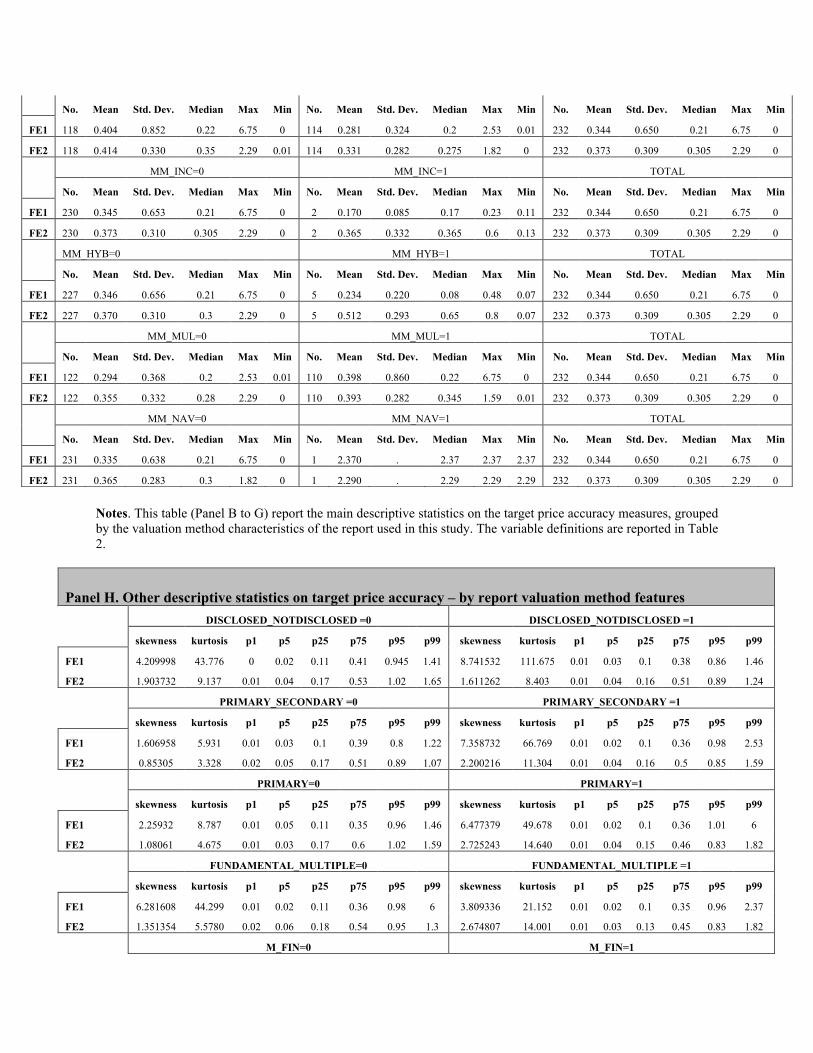
Notes. This table (Panel B to G) report the main descriptive statistics on the target price accuracy measures, grouped by the valuation method characteristics of the report used in this study. The variable definitions are reported in Table 2.

Panel H. Other descriptive statistics on target price accuracy – by report valuation method features DISCLOSED_NOTDISCLOSED =0 DISCLOSED_NOTDISCLOSED =1

skewness kurtosis p1 p5 p25 p75 p95 p99 skewness kurtosis p1 p5 p25 p75 p95 p99

FE1 4.209998 43.776 0 0.02 0.11 0.41 0.945 1.41 8.741532 111.675 0.01 0.03 0.1 0.38 0.86 1.46

FE2 1.903732 9.137 0.01 0.04 0.17 0.53 1.02 1.65 1.611262 8.403 0.01 0.04 0.16 0.51 0.89 1.24

PRIMARY_SECONDARY =0 PRIMARY_SECONDARY =1


FE1 1.606958 5.931 0.01 0.03 0.1 0.39 0.8 1.22 7.358732 66.769 0.01 0.02 0.1 0.36 0.98 2.53

FE2 0.85305 3.328 0.02 0.05 0.17 0.51 0.89 1.07 2.200216 11.304 0.01 0.04 0.16 0.5 0.85 1.59

PRIMARY=0 PRIMARY=1


FE1 2.25932 8.787 0.01 0.05 0.11 0.35 0.96 1.46 6.477379 49.678 0.01 0.02 0.1 0.36 1.01 6

FE2 1.08061 4.675 0.01 0.03 0.17 0.6 1.02 1.59 2.725243 14.640 0.01 0.04 0.15 0.46 0.83 1.82

FUNDAMENTAL_MULTIPLE=0 FUNDAMENTAL_MULTIPLE =1


FE1 6.281608 44.299 0.01 0.02 0.11 0.36 0.98 6 3.809336 21.152 0.01 0.02 0.1 0.35 0.96 2.37

FE2 1.351354 5.5780 0.02 0.06 0.18 0.54 0.95 1.3 2.674807 14.001 0.01 0.03 0.13 0.45 0.83 1.82

M_FIN=0 M_FIN=1


FE1 118 0.404 0.852 0.22 6.75 0 114 0.281 0.324 0.2 2.53 0.01 232 0.344 0.650 0.21 6.75 0

FE2 118 0.414 0.330 0.35 2.29 0.01 114 0.331 0.282 0.275 1.82 0 232 0.373 0.309 0.305 2.29 0

MM_INC=0 MM_INC=1 TOTAL


FE1 230 0.345 0.653 0.21 6.75 0 2 0.170 0.085 0.17 0.23 0.11 232 0.344 0.650 0.21 6.75 0

FE2 230 0.373 0.310 0.305 2.29 0 2 0.365 0.332 0.365 0.6 0.13 232 0.373 0.309 0.305 2.29 0

MM_HYB=0 MM_HYB=1 TOTAL


FE1 227 0.346 0.656 0.21 6.75 0 5 0.234 0.220 0.08 0.48 0.07 232 0.344 0.650 0.21 6.75 0

FE2 227 0.370 0.310 0.3 2.29 0 5 0.512 0.293 0.65 0.8 0.07 232 0.373 0.309 0.305 2.29 0

MM_MUL=0 MM_MUL=1 TOTAL


FE1 122 0.294 0.368 0.2 2.53 0.01 110 0.398 0.860 0.22 6.75 0 232 0.344 0.650 0.21 6.75 0

FE2 122 0.355 0.332 0.28 2.29 0 110 0.393 0.282 0.345 1.59 0.01 232 0.373 0.309 0.305 2.29 0

MM_NAV=0 MM_NAV=1 TOTAL


FE1 231 0.335 0.638 0.21 6.75 0 1 2.370 . 2.37 2.37 2.37 232 0.344 0.650 0.21 6.75 0

FE2 231 0.365 0.283 0.3 1.82 0 1 2.290 . 2.29 2.29 2.29 232 0.373 0.309 0.305 2.29 0


FE1 8.186869 86.807 0.01 0.03 0.11 0.42 0.86 1.49 3.166292 19.812 0.01 0.02 0.09 0.34 0.87 1.33

FE2 1.682951 10.181 0.03 0.07 0.2 0.56 0.85 1.08 1.594552 6.823 0.01 0.03 0.14 0.46 0.9 1.24

M_INC=0 M_INC=1


FE1 8.719091 110.884 0.01 0.02 0.1 0.38 0.87 1.46 1.685403 4.402 0.1 0.1 0.11 0.29 0.76 0.76

FE2 1.635258 8.5016 0.01 0.04 0.16 0.5 0.9 1.24 -0.5852587 1.801 0.13 0.13 0.16 0.7 0.76 0.76

M_NAV=0 M_NAV=1


FE1 9.255953 121.626 0.01 0.02 0.1 0.38 0.84 1.26 2.234125 7.470 0.04 0.09 0.12 0.4 1.49 2.37

FE2 1.282099 5.634 0.01 0.04 0.16 0.5 0.85 1.17 2.373052 9.999 0.15 0.24 0.39 0.84 1.04 2.29

M_HYB=0 M_HYB=1


FE1 8.68665 109.91 0.01 0.03 0.1 0.38 0.87 1.46 0.7789851 2.034 0.02 0.02 0.07 0.36 0.53 0.53

FE2 1.630386 8.442 0.01 0.04 0.16 0.51 0.9 1.24 0.0693842 2.229 0.07 0.07 0.27 0.57 0.8 0.8

M_MUL=0 M_MUL=1


FE1 3.599761 19.076 0.01 0.02 0.075 0.38 0.97 2.53 9.293103 119.2 0.01 0.03 0.1 0.38 0.84 1.43

FE2 2.823189 14.014 0 0.02 0.14 0.445 0.97 2.29 0.9911456 4.035 0.02 0.05 0.17 0.535 0.88 1.08

MM_FIN=0 MM_FIN=1


FE1 6.099276 42.883 0.01 0.02 0.1 0.39 1.02 6 3.774152 23.224 0.01 0.02 0.1 0.34 0.96 1.33

FE2 2.245488 11.664 0.02 0.06 0.18 0.57 1.02 1.59 2.021524 9.552 0.01 0.02 0.13 0.44 0.83 1.24

MM_INC=0 MM_INC=1


FE1 7.34038 66.456 0.01 0.02 0.1 0.36 0.98 2.53 0 1 0.11 0.11 0.11 0.23 0.23 0.23

FE2 2.189838 11.2405 0.01 0.04 0.16 0.5 0.85 1.59 0 1 0.13 0.13 0.13 0.6 0.6 0.6

MM_HYB=0 MM_HYB=1


FE1 7.309883 65.801 0.01 0.02 0.11 0.35 0.98 2.53 0.4079907 1.168 0.07 0.07 0.07 0.47 0.48 0.48

FE2 2.240929 11.501 0.01 0.04 0.16 0.49 0.85 1.59 -0.6554944 1.979 0.07 0.07 0.37 0.67 0.8 0.8

MM_NAV=0 MM_NAV=1


FE1 7.748807 72.716 0.01 0.02 0.1 0.35 0.97 2.53 . . 2.37 2.37 2.37 2.37 2.37 2.37

FE2 1.598129 7.093 0.01 0.04 0.16 0.5 0.85 1.3 . . 2.29 2.29 2.29 2.29 2.29 2.29

MM_MUL=0 MM_MUL=1


FE1 3.791858 20.984 0.01 0.02 0.1 0.35 0.96 2.37 6.281608 44.299 0.01 0.02 0.11 0.36 0.98 6

FE2 2.669866 13.913 0.01 0.03 0.13 0.45 0.83 1.82 1.351354 5.578 0.02 0.06 0.18 0.54 0.95 1.3 Notes. Panel G reports other descriptive statistics on the target price accuracy measures, grouped by the valuation method characteristics of the report used in this study. The variable definitions are reported in Table 2.

Table 4. Descriptive statistics of the control variables of the models

2007

BOLDNESS FORAGE PMAFE VOL GROWTH SIZE NAZ No. 168 132 132 171 171 171 147 Mean 0.22 190.90 0.02 4.31 2.71 10.81 0.69 Std. Dev. 0.34 95.55 0.54 3.53 1.69 0.45 0.46 Median 0.14 192 0 3.45 2.18 10.87 - Max 1.61 354 1.72 13.69 7.69 11.6 1 Min -0.16 21 -0.97 0.12 1.18 9.45 0 Skewness 2.67 0.01 0.67 0.79 1.69 -0.93 -0.84 Kurtosis 10.34 1.85 3.34 2.48 4.80 4.03 1.71 p1 -0.13 24 -0.95 0.12 1.29 9.45 0 p5 -0.06 46 -0.83 0.76 1.34 9.91 0 p25 0.03 103.5 -0.4 1.31 1.51 10.6 0 p75 0.29 257 0.295 7.04 3.15 11.12 1 p95 1.2 340 0.97 11.42 7.06 11.45 1 p99 1.6 353 1.46 12.88 7.66 11.57 1

2008 BOLDNESS FORAGE PMAFE VOL GROWTH SIZE NAZ

No. 753 671 681 813 805 805 774 Mean 0.36 100.97 0.01 6.10 1.85 10.33 0.39 Std. Dev. 0.33 71.00 0.52 5.77 1.27 0.64 0.49 Median 0.3 85 0.02 4.43 1.38 10.4 - Max 2.95 358 4.41 24.29 6.55 11.67 1 Min -0.37 0 -1 0.33 0.26 7.63 0 Skewness 1.993 1.440 2.359 1.734 1.443 -1.075 0.450 Kurtosis 12.627 5.413 17.081 5.663 4.681 4.687 1.203 p1 -0.18 8 -0.95 0.33 0.35 8.24 0 p5 -0.07 16 -0.77 0.62 0.51 9.2 0 p25 0.16 52 -0.24 2.08 0.93 10.01 0 p75 0.5 146 0.17 8.46 2.36 10.79 1 p95 0.89 272 0.63 20.4 4.58 11.17 1 p99 1.45 342 2.13 24.29 6.12 11.37 1

2009 BOLDNESS FORAGE PMAFE VOL GROWTH SIZE NAZ

No. 614 557 550 666 663 663 643 Mean 0.31 306.29 0.00 3.97 1.30 9.99 0.35 Std. Dev. 0.34 30.06 0.54 3.33 0.87 0.75 0.48 Median 0.27 308 -0.01 2.495 1.12 10.04 - Max 3.12 359 6.46 11.32 4.16 11.51 1 Min -0.55 160 -1 0.09 0.03 5.71 0 Skewness 1.782 -0.774 3.522 0.861 1.284 -1.511 0.622 Kurtosis 12.188 5.020 39.603 2.547 4.418 8.666 1.387 p1 -0.3 208 -0.95 0.09 0.2 7.87 0 p5 -0.12 259 -0.77 0.38 0.35 8.55 0 p25 0.1 287 -0.3 1.27 0.68 9.68 0 p75 0.47 328 0.25 5.91 1.73 10.39 1 p95 0.93 353 0.74 11.24 3.2 11.04 1 p99 1.33 358 1.58 11.32 3.9 11.46 1

Total BOLDNESS FORAGE PMAFE VOL GROWTH SIZE NAZ

No. 1535 1360 1363 1650 1639 1639 1564 Mean 0.32 193.79 0.01 5.05 1.72 10.24 0.40 Std. Dev. 0.34 114.79 0.53 4.82 1.26 0.71 0.49 Median 0.27 170 0 3.81 1.36 10.3 - Max 3.12 359 6.46 24.29 7.69 11.67 1 Min -0.55 0 -1 0.09 0.03 5.71 0 Skewness 1.924 -0.092 2.690 39.751 1.781 -1.292 0.396 Kurtosis 11.816 1.411 25.619 1603.309 6.787 7.018 1.157 p1 -0.24 12 -0.95 0.12 0.29 8.11 0 p5 -0.09 26.5 -0.77 0.47 0.395 8.96 0 p25 0.11 78 -0.28 1.76 0.87 9.91 0 p75 0.46 307 0.21 7.04 2.135 10.75 1 p95 0.92 343 0.74 12.88 4.33 11.18 1 p99 1.45 356 1.82 24.29 6.47 11.47 1

Notes. This table reports the descriptive statistics (grouped by year and reported in total) of the control variables used in the different model specifications. Specifically, as reported in Table 2, BOLDNESS is the target price boldness and is measured as the absolute value of the difference between the target price and the current price scaled by current price; VOL indicates the market price volatility measured as the standard deviation of company prices for each of the three years considered; SIZE indicates the natural logarithm of the firm’s market capitalization at the report issuing date; GROWTH is the company price-to-book-value ratio; PMAFE is the Proportional Mean Absolute Forecast Error and is the earnings forecast accuracy measure. It is computed as:

(-1)

It measures the difference between the absolute forecast error (AFE) of analyst i forecasting earnings for firm j in the fiscal year t and the average absolute forecast error across all analyst forecasts of firm j’s fiscal year t earnings, expressed as a fraction of the average absolute forecast error across all analyst forecasts of firm j’s fiscal year t earnings. PMAFE controls for firm-year effects by subtracting the mean absolute forecast error, AAFE , from the analyst’s absolute forecast error. Deflating by AAFE reduces heteroskedasticity in forecast error distributions across firms (Clement (1999)). Multiplying by -1 ensures that higher values for PMAFE correspond to higher levels of accuracy. FORAGE is the time interval (in number of days) between the forecast date and the fiscal year end, while NAZ is a dummy variable equal to 1 whether the analyst’s nationality coincides with the company nationality, 0 otherwise.

Table 5. Descriptive statistics on the main independent variables of the models

Year DISCLOSED_NOTDISCLOSED PRIMARY_SECONDAR

Y PRIMAR

Y FUNDAMENTAL_MULTIPLE MM_FIN MM_INC MM_HYB

2007 No. 166 85 33 33 33 33 33

%

(=1) 51.20% 38.82% 39.39% 33.33% 21.21% 3.03% 9.09%

2008 No. 746 258 90 91 90 90 90

%

(=1) 34.18% 34.50% 68.89% 60.44% 55.56% 0.00% 3.33%

2009 No. 612 262 111 111 111 111 111

%

(=1) 41.99% 42.37% 72.97% 52.25% 51.35% 0.90% 0.00%

Total No. 1524 605 234 235 234 234 234

%

(=1) 39.17% 38.51% 66.67% 52.77% 48.72% 0.85% 2.56%

Year MM_NAV MM_MRATIO M_FIN M_INC M_NAV M_HYB M_MRATIO

2007 No. 33 33 85 85 85 85 85

%

(=1) 0.00% 66.67% 50.59% 2.35% 12.94% 4.71% 91.76%

2008 No. 90 90 255 255 255 255 255

%

(=1) 1.11% 40.00% 43.53% 1.18% 3.14% 2.75% 80.78%

2009 No. 111 111 257 257 257 257 257

%

(=1) 0.00% 47.75% 46.30% 0.78% 3.50% 2.33% 83.27%

Total No. 234 234 597 597 597 597 597

%

(=1) 0.43% 47.44% 45.73% 1.17% 4.69% 2.85% 83.42% Notes. This table reports the descriptive statistics (grouped by year and reported in total) of the main independent variables of the models. They synthesize the report valuation methods features. Specifically, as reported in Table 2, DISCLOSED_NOTDISCLOSED is a dummy variable assuming value equal to 1 whether in the report has a distinguishable valuation method, 0 otherwise. PRIMARY_SECONDARY is equal to 1 if there’s a primary valuation method, 0 otherwise; the PRIMARY variable is equal to 1 if the analyst uses just that method to evaluate the company, 0 if the method is chosen as primary in a group of other secondary methods; M_FIN, M_INC, M_NAV, M_HYB, M_MRATIO indicate different methods categories, respectively financial methods, income-based ones, net asset methods, hybrid and market ratios methods. Each variable is a dummy assuming value 1 in correspondence to the category it represents, 0 otherwise; FUNDAMENTAL_MULTIPLE is a variable assuming value equal to 1 if the analyst uses an absolute method (such as a financial method, an income based method, a hybrid or a net asset method, 0 if he/she uses a market ratios approach).;MM_FIN, MM_INC, MM_NAV, MM_HYB, MM_MRATIO are dummy variables representing the main valuation method used by the analyst. Each one is equal to 1 whether the analyst uses that specific method as main valuation method.

Table 6. The correlation matrix among variables.

Panel A - The Pearson’s correlation.

FE1 FE2 DISCLOSED_NOTDISCLOSED PRIMARY_SECONDARY PRIMARY M_FIN M_INC M_NAV M_MRATIO M_HYB

FE1 1

FE2 0.4617* 1

DISCLOSED _NOTDISCLOSED

-0,0148 -0.0551*

1

PRIMARY _SECONDARY

0,064 0,0034 0.1026* 1

PRIMARY

0,0624 -0,0883 1

M_FIN -0.0785*

-0.0857*

0.1665* -0.3348* 1

M_INC -0,0102 0,047 -0,0237 -0.1313* -0.0687*

1

M_NAV 0,0644 0.2069* 0,0494 -0.3185* -0.0923*

0.1230* 1

M_MRATIO -0,0017 0,0217 -0.3165* -0.4761* -0.4315*

0,0486 0,035 1

M_HYB -0,0384 0,0258 -0,0057 -0,0887 -0,0359 -0,0186 0.1526* -0.0861* 1

FUNDAMENTAL _MULTIPLE

-0,0814 -0,0606 -0.1634* 0.7701* 0,0877 -0.1940*

-0.6351* 0.1658*

MM_FIN -0,0953 -0.1338*

-0.1270* 0.8643* -0,0905 -0.2098*

-0.6170* -0,121

MM_INC -0,0249 -0,0025 -0.1313* -0,1047 1.0000* -0,0234 0,0625 -0,0163

MM_MRATIO 0,0804 0,0614 0.1634* -0.7782*

-0,0882 0.1934* 0.6397* -0.1668*

MM_HYB -0,0251 0,0667 -0,0574 -0.1829*

-0,0151 -0,0409 -0,0658 0.9238*

BOLD 0.3770* 0.3416* -0.1293* -0,0341 0,0248 -0,0541 -0,0493 0,0657 0,0245 0,0629

FORAGE 0.0921* -0,0162 0.0888* 0.0758* -0,0155 0,0075 0,0326 0,0188 0,0491 0,0496

PMAFE 0,0262 0.1035* -0.0492* 0 0,0479 0,0117 -0,0187 -0,0199 -0,0485 -0.0582

VOL 0.0569* 0.1883* -0,028 0,0581 -0,0813 -0.1411*

-0,0119 0,0607 0,0495 -0.0462

GROWTH -0.2277*

-0.1749*

0.0886* 0,0666 -0,0469 0.1488* 0,0012 -0.0904*

-0,0519 -0.0697*

SIZE -0.3878*

-0.1898*

-0,0288 -0,0016 -0.1333* 0,0619 0.0696* -0,0379 0,0341 0,0226

NAZ 0,021 0.0830* -0.1279* -0.0797* -0.1698* -0,0036 -0,0001 0.0973* 0.0842* 0,0319

Panel B - The Pearson’s correlation.


MM_FIN MM_INC MM_MRATIO MM_HYB BOLD FORAGE PMAFE VOL GROWTH SIZE NAZ


1

MM_FIN 0.9259* 1

MM_INC 0,0882 -0,0905 1

MM_MRATIO -1 -0.9259* -0,0882 1

MM_HYB 0.1541* -0.1581* -0,0151 -0.1541* 1

BOLD 0,0066 0,0058 -0,0429 -0,0074 0,008 1

FORAGE -0,0599 -0,0584 -0,046 0,0576 0,0659 -0.0916*

1

PMAFE 0,0799 0,1059 -0,0783 -0,0799 -0,0489 0,0311 0.1270* 1

VOL -0.1253* -0.1270* -0,0749 0.1257* 0,043 0.0460* -0.1249* 0,0109 1

GROWTH 0,0968 0.1240* -0,0085 -0,0945 -0,052 -0.2329*

-0.1227* 0.0471* -0.0992*

1

SIZE 0,0171 -0,0117 0,0322 -0,0175 0.1627* -0.1479*

-0.1472* 0.0742* 0,022 0.3878* 1

NAZ -0,1027 -0.1670* 0,0427 0,1027 0.1814* 0.1060* -0,0027 0,0297 0.0898* -0.0542* 0.0569* 1

Notes. These panels (A and B – Table 6) report the correlation matrix of the different model specification variables. It is based on the Pearson’s correlation definition. Some of the correlations are missing because of the variables definition. All the variables have been defined above. * denotes significance at the 10%

Table 7. The correlation matrix among variables.

Panel A - The Spearman’s correlation.

FE1 FE2 DISCLOSED_ NOTDISCLOSED

PRIMARY _SECONDARY

PRIMARY M_FIN M_INC M_NAV M_MRATIO M_HYB

FE1 1

FE2 0.4955* 1

DISCLOSED_ NOTDISCLOSED

-0.0569* -0,0403 1

PRIMARY _SECONDARY

-0,0014 -0,0298 0.1026* 1

PRIMARY -0,0125 -0.1155*

. . 1

M_FIN -0.0721* -0.1164*

. 0.1665* -0.3348* 1

M_INC 0,0001 0,061 . -0,0237 -0.1313* -0.0687*

1

M_NAV 0,0551 0.1770* . 0,0494 -0.3185* -0.0923*

0.1230* 1

M_MRATIO 0,0128 0,0651 . -0.3165* -0.4761* -0.4315*

0,0486 0,035 1

M_HYB -0,0572 0,0476 . -0,0057 -0,0887 -0,0359 -0,0186 0.1526* -0.0861* 1


-0,0613 -0,1056 . . -0.1634* 0.7701* 0,0877 -0.1940* -0.6351* 0.1658*

MM_FIN -0,0611 -0.1505*

. . -0.1270* 0.8643* -0,0905 -0.2098* -0.6170* -0.1210*

MM_INC -0,0321 0,0041 . . -0.1313* -0,1047 1.0000* -0,0234 0,0625 -0,0163

MM_MRATIO 0,0594 0,108 . . 0.1634* -0.7782*

-0,0882 0.1934* 0.6397* -0.1668*

MM_HYB -0,0282 0,0896 . . -0,0574 -0.1829*

-0,0151 -0,0409 -0,0658 0.9238*

BOLD 0.3102* 0.1991* -0.1515* -0,0356 -0,0018 -0,0623 -0,0605 0.0691* 0,0311 0,0577

FORAGE 0.0779* 0,0007 0.0730* 0,057 -0,009 -0,006 0,0264 0,0157 0,044 0,0518

PMAFE 0,0095 0.0926* -0.0544* -0,0287 0,0547 -0,0156 -0,0023 -0,0204 -0,0198 -0,0648

VOL 0.0527* 0.1335* -0,0081 0.0791* -0.1091* -0.1276*

-0,0157 0,0243 0,0578 -0,0548

GROWTH -0.2836* -0.1905*

0.1166* 0.1231* -0.1242* 0.2087* 0,0374 -0.0799* -0.0699* -0,0456

SIZE -0.2034* -0.0690*

-0,0379 0,012 -0.1256* 0,0394 0.0797* 0,0309 0,0349 0,0438

NAZ 0,0274 0.0960* -0.1279* -0.0797* -0.1698* -0,0036 -0,0001 0.0973* 0.0842* 0,0319

Panel B - The Spearman’s correlation.


MM_FIN MM_INC MM_MRATIO MM_HYB BOLD FORAGE PMAFE VOL GROWTH SIZE NAZ


1

MM_FIN 0.9259* 1

MM_INC 0,0882 -0,0905 1

MM_MRATIO -1 -0.9259* -0,0882 1

MM_HYB 0.1541* -0.1581* -0.0151 -0.1541* 1

BOLD 0,0364 0,0321 -0,0592 -0,0372 0,0163 1

FORAGE -0,0429 -0,0528 -0,0554 0,0419 0,0988 -0.0950*

1

PMAFE 0,0838 0,1013 -0,0694 -0,0839 -0,0411 0.0596* 0.1731* 1

VOL -0.1451* -0.1572* -0,095 0.1473* 0,0696 -0,0152 -0.0644* 0,0442 1

GROWTH 0,1052 0.1183* 0,0219 -0,1019 -0,0099 -0.2847*

-0.1018* 0.0954* 0,02 1

SIZE -0,0077 -0,0613 0,0275 0,0064 0.2028* -0.0782*

-0.1435* 0.1324* 0,0377 0.4842* 1

NAZ -0,1027 -0.1670* 0,0427 0,1027 0.1814* 0.1249* 0,0002 0,0086 0.0971* -0.0666* 0.0827* 1

Notes. These panels (A and B – Table 7) report the correlation matrix among of the different model specification variables. It is based on the Spearman’s correlation definition. Some of the correlations are missing because of the variables definition. All the variables have been defined above. * denotes significance at the 10%

Table 8. The effect on the target price accuracy of the valuation methods disclosure (1) (2) (3) (4)

VARIABLES FE1 FE1 FE1 FE1

BOLD 0.364*** 0.394*** 0.386***

(0) (0) (0)

FORAGE 0.000255 0.000280*

(0.109) (0.0907)

PMAFE 0.0267 0.0155

(0.125) (0.440)

VOL 0.00294 0.00376

(0.238) (0.152)

GROWTH 0.0917*** 0.0996*** 0.0898***

(9.43e-08) (1.26e-08) (2.31e-10)

SIZE -0.346*** -0.348*** -0.311***

(0) (0) (0)

D_2008 -0.109*** -0.0973**

(0.00358) (0.0118)

D_2009 -0.103** -0.0823*

(0.0250) (0.0816)

NAZ -0.00682 0.00402

(0.736) (0.849)

DISCLOSED_NOTDISCL

OSED

-0.0109 0.0277 0.0270

(0.599) (0.165) (0.129)

Constant 0.321*** 3.623*** 3.578*** 3.209***

(0.0000) (0.0000) (0.0000) (0.0000)

Observations 1,424 1,275 1,213 1,424

R-squared 0.000 0.287 0.298 0.281

Number of sector 20 20 20 20

pval in parentheses

*** p<0.01, ** p<0.05, * p<0.1

Notes. This table reports the main results of equation (5), testing the effect on the target price accuracy of the valuation methods disclosure. Table 2 defines all the variables used.

Table 9. The effect on the target price accuracy of the valuation method hierarchy

disclosure (1) (2) (3) (4)


BOLD 0.364*** 0.384*** 0.371***

(0) (5.15e-10) (2.02e-10)

FORAGE 0.000255 0.000294

(0.109) (0.265)

PMAFE 0.0267 -0.00885

(0.125) (0.794)

VOL 0.00294 0.0107**

(0.238) (0.0231)

GROWTH 0.0917*** 0.129*** 0.117***

(9.43e-08) (1.71e-05) (2.50e-06)

SIZE -0.346*** -0.464*** -0.427***

(0.0000) (0.0000) (0.0000)

D_2008 -0.109*** -0.109*

(0.00358) (0.0702)

D_2009 -0.103** -0.110

(0.0250) (0.141)

NAZ -0.00682 -0.00534

(0.736) (0.888)

PRIMARY_SECONDARY 0.110*** 0.104*** 0.116***

(0.00635) (0.00300) (0.000514)

Constant 0.266*** 3.623*** 4.656*** 4.305***

(0.0000) (0.0000) (0.0000) (0.0000)

Observations 592 1,275 541 592

R-squared 0.013 0.287 0.360 0.334


pval in parentheses

*** p<0.01, ** p<0.05, * p<0.1

Notes. This table reports the main results of equation (6), testing the effect on the target price accuracy of the valuation methods hierarchy disclosure. Table 2 defines all the variables used.

Table 10. The effect on the target price accuracy of the main and unique valuation method

disclosure (1) (2) (3) (4)


BOLD 0.364*** 0.805*** 0.821***

(0) (0) (0)

FORAGE 0.000255 6.51e-06

(0.109) (0.988)

PMAFE 0.0267 0.0133

(0.125) (0.815)

VOL 0.00294 0.00405

(0.238) (0.655)

GROWTH 0.0917*** 0.235*** 0.178***

(9.43e-08) (1.90e-05) (2.38e-05)

SIZE -0.346*** -0.747*** -0.684***

(0) (0) (0)

D_2008 -0.109*** -0.193*

(0.00358) (0.0622)

D_2009 -0.103** -0.0654

(0.0250) (0.580)

NAZ -0.00682 0.184***

(0.736) (0.00839)

PRIMARY 0.101 -0.0723 -0.0543

(0.289) (0.237) (0.343)

Constant 0.277*** 3.623*** 7.400*** 6.805***

(0.000285) (0) (0) (0)


R-squared 0.005 0.287 0.694 0.650


pval in parentheses *** p<0.01, ** p<0.05, * p<0.1

Notes. This table reports the main results of equation (7), testing the effect on the target price accuracy of the main and unique valuation method disclosure. Table 2 defines all the variables used.

Table 11. The effect on the target price accuracy of different valuation methods (1) (2) (3) (4)


BOLD 0.364*** 0.396*** 0.382***

(0) (4.66e-10) (1.55e-10)

FORAGE 0.000255 0.000292

(0.109) (0.282)

PMAFE 0.0267 -0.0114

(0.125) (0.745)

VOL 0.00294 0.0111**

(0.238) (0.0227)

GROWTH 0.0917*** 0.127*** 0.108***

(9.43e-08) (3.35e-05) (1.87e-05)

SIZE -0.346*** -0.459*** -0.418***

(0) (0) (0)

D_2008 -0.109*** -0.119*

(0.00358) (0.0561)

D_2009 -0.103** -0.104

(0.0250) (0.185)

NAZ -0.00682 -0.0132

(0.736) (0.737)

M_FIN -0.0198 -0.00885 -0.0163

(0.678) (0.839) (0.681)

M_INC -0.157 0.0214 0.00813

(0.363) (0.892) (0.955)

M_NAV 0.174* 0.112 0.190**

(0.0961) (0.249) (0.0290)

M_MRATIO -0.0657 -0.0534 -0.0503

(0.257) (0.301) (0.295)

M_HYB -0.311** -0.0594 -0.106

(0.0161) (0.636) (0.328)

Constant 0.375*** 3.623*** 4.690*** 4.319***

(4.62e-09) (0) (0) (0)


R-squared 0.016 0.287 0.353 0.329



Notes. This table reports the main results of equation (8), testing the effect on the target price accuracy of different valuation methods used. Table 2 defines all the variables used.

Table 12. The effect on the target price accuracy of the “absolute” and “relative” valuation

methods (1) (2) (3) (4)


BOLD 0.364*** 0.807*** 0.826***

(0) (0) (0)

FORAGE 0.000255 -3.09e-05

(0.109) (0.944)

PMAFE 0.0267 0.0220

(0.125) (0.704)

VOL 0.00294 0.00452

(0.238) (0.618)

GROWTH 0.0917*** 0.228*** 0.175***

(9.43e-08) (2.96e-05) (2.52e-05)

SIZE -0.346*** -0.739*** -0.678***

(0) (0) (0)

D_2008 -0.109*** -0.203**

(0.00358) (0.0488)

D_2009 -0.103** -0.0641

(0.0250) (0.589)

NAZ -0.00682 0.185***

(0.736) (0.00812)

FUNDAMENTAL

_MULTIPLE

-0.0607 -0.0631 -0.0954

(0.549) (0.360) (0.115)

Constant 0.375*** 3.623*** 7.328*** 6.756***

(7.45e-08) (0) (0) (0)


R-squared 0.002 0.287 0.693 0.653



Notes. This table reports the main results of equation (9), testing the effect on the target price accuracy of “absolute” and “relative” valuation methods. Table 2 defines all the variables used.

Table 13. The effect on the target price accuracy of different kinds of main valuation

methods (1) (2) (3) (4) (5)

VARIABLES FE1 FE1 FE1 FE1 FE1

MM_FIN -0.923** 0.0709 0.228 -0.104

(0.0364) (0.738) (0.407) (0.102)

MM_INC -1.152** -0.157 -0.228 -0.332

(0.0249) (0.639) (0.407) (0.220)

MM_MRATIO -0.820* 0.175 0.104 0.332

(0.0601) (0.407) (0.102) (0.220)

MM_HYB -0.994** -0.0709 0.157 -0.175

(0.0441) (0.738) (0.639) (0.407)

MM_NAV 0.994** 0.923** 1.152** 0.820*

(0.0441) (0.0364) (0.0249) (0.0601)

BOLD 0.836*** 0.836*** 0.836*** 0.836*** 0.836***

(0) (0) (0) (0) (0)

GROWTH 0.175*** 0.175*** 0.175*** 0.175*** 0.175***

(2.99e-05) (2.99e-05) (2.99e-05) (2.99e-05) (2.99e-05)

SIZE -0.658*** -0.658*** -0.658*** -0.658*** -0.658***

(0) (0) (0) (0) (0)

Constant 7.380*** 6.386*** 6.457*** 6.229*** 6.560***

(0) (0) (0) (0) (0)

Observations 232 232 232 232 232

R-squared 0.662 0.662 0.662 0.662 0.662

Number of sector 20 20 20 20 20


Notes. This table reports the main results of equation (10), testing the effect on the target price accuracy of different types of main valuation methods used. Table 2 defines all the variables used.

Graphs

Graph 1. Target Price Accuracy across sectors

Graph 2. Target Price Accuracy across different recommendation categories

Graph 3. Percentage of different categories of valuation approaches over the years

Graph 4. Percentage of different kinds of methods over the years

Graph 5. Percentage of different categories of methods across sectors

References

ASQUITH P., MIKHAIL M., AU A. (2005): “Information content of equity analyst reports”, in Journal

of Financial Economics, 75 , pp. 245-282.

BARKER R. (1998) “The market for information: Evidence from Finance Director, Analysts and Fund

Managers”, Accounting and Business Research, 29, 3-20.

BAKER R. (1999), “The role of dividends in valuation models used by analysts and fund managers”, The

European Accounting Review, 8 (2):195-218.

BERTINETTI G., CAVEZZALI E., RIGONI U. (2006): “The content of reports on Italian stocks. Do

evaluation methods matter?”, EFMA Madrid Meetings Working Paper.

BLOCK S. (1999), “A Study of Financial Analysts: Practice and Theory”, Financial Analysts Journal,

55 (4): 86-95.

BONINI S., ZANETTI L., BIANCHINI R. and SALVI A. (2009), “Target Price Accuracy in Equity

Research”, Working Paper. http://papers.ssrn.com/sol3/papers.cfm?abstract_id=676327

BOLLIGER, G, (2004) “The characteristics of individual analysts' forecasts in Europe”, Journal of

Banking and Finance 28, 2283-2309

BRADSHAW M. T. (2002): “The use of target price to justify sell-side analysts’ stock

recommendations”, in Accounting Horizons, 16 No 1, pp. 27-41.

BRADSHAW M. and BROWN L. (2004), “How Do Analysts Use Their Earning Forecasts in

Generating Stock Recommendations?”, The Accounting Review, 79 (1): 25- 50.

BRADSHAW M. and BROWN L. (2006), “Do Sell-Side Analysts Exhibit Differencial Target Price

Forecasting Ability?”, Working paper. http://papers.ssrn.com/sol3/papers.cfm?abstract_id=698581

BRAV A., LEHAVY R. (2003): “An empirical analysis of analysts’ target prices: short term

informativeness and long term dynamics”, in The Journal of Finance, 58 (5), pp. 1933-1967.

BROWN L. (2001), “How Important Is Past Analyst Forecast Accuracy?”, Financial Analysts Journal,

57 (6): 44-49.

DAMODARAN A. (2001): The dark side of valuation: valuing old tech, new tech and new economy

companies, Prentice Hall.

DE VINCENTIIS (2010), “Accuratezza e distorsione delle previsioni degli analisti finanziari in un

contesto di elevata trasparenza. Una verifica empirica nel mercato italiano”, Bancaria, 3: 31-51.

DEMIRAKOS E., STRONG N. and WALKER M: (2004), “What Valuation Models Do Analysts Use?”,

Accounting Horizons, 18 (4): 221-240.

DEMIRAKOS E., STRONG N. and WALKER M (2009), “Does valuation model choice affect target

price accuracy?”, Working Paper. http://papers.ssrn.com/sol3/papers.cfm?abstract_id=1370847

FRANCIS J. and SOFFER L.(1997), “The relative Informativeness of Analysts’ Stock

Recommendations and Earning Forecast Revisions”, Jounal of Accounting Research, 35 (2): 193-211.

GLEASON C., JOHNSON B. and LI H. (2006), “The Earning Forecast Accuracy, Valuation Model Use,

and Price Target Performance of Sell-Side Equity Analysts”, Working Paper.

http://www.nd.edu/~carecob/Paper%20Links/Su'06%20Conf/Gleason%206-06.pdf

GLEASON C., JOHNSON B. and LI H. (2008), “Valuation Model Use and the Price Target

Performance of Sell-Side Equity Analysts”, Working Paper.

http://papers.ssrn.com/sol3/papers.cfm?abstract_id=930720

GLEASON C., LEE C. (2003): “Analyst forecast revisions and market price discovery”, in The

Accounting Review, 78 (1), pp. 193-225.

GLEASON C., LEE C. (2000): “Characteristics of price informative analyst forecast”, University of

Iowa - Department of Accounting and Cornell University - Samuel Curtis Johnson Graduate School of

Management. http://papers.ssrn.com/sol3/papers.cfm?abstract_id=254563

HILL & KNOWLTON (1984). The annual report: A question of credibility. New York: Hill and

Knowlton

IMAM, S., BARKER, R., CLUBB C. (2008) The use of valuation models by UK investment

analysts, European Accounting Review, 17, pp. 503–535.

KOLLER, T., GOEDHART, M., WESSEL, D. (2005) Valuation: Measuring and Managing the

Value of Companies. New York: John Wiley and Sons.

PENMAN S. (2001), Financial Statement Analysis and Security Valuation, McGraw-Hill International

Edition, New York.

PREVITS. G., BRICKER R., ROBINSON T. and YOUNG S. (1994), “ A content analysis of sell-side

financial analyst company reports”, Accounting Horizons, 8 (2): 55-70.

financial analysts accuracy do valuation methods matter

Documents