Meghana Ayyagari

Thorsten Beck

Mohammad Hoseini

Finance and Poverty:

Evidence from India

Motivation Large literature on positive effect of finance and growth

Distributional repercussions of financial deepening?

Theory ambiguous: Credit constraints are particularly binding for the poor (Banerjee and

Newman,1993; Galor and Zeira, 1993; Aghion and Bolton, 1997)

Finance helps overcome barriers of indivisible investment (McKinnon, 1973)

Only rich can pay “entry fee” into financial system (Greenwood and Jovanovic, 1993)

Credit is channeled to incumbent and connected and not to entrepreneurs with best opportunities (Lamoreaux, 1986; Haber, 1991)

Cross-country-level: Beck, Demirguc-Kunt and Levine (2007),

but challenges of

Identification

Measurement

Channels

Beck, Demirguc-Kunt and Levine (2007)

Questions remain

Correlation or causality?

Identification strategies on cross-country level have limitation

Mechanisms Financial deepening alleviates credit constraints on the poor allowing

them accumulate human capital Galor and Zeira (1993)

Financial deepening alleviates credit constraints on the poor allowing them to become entrepreneurs and realize profitable projects Banerjee and Newman (1993)

Muhamed Yunus (Grameen Bank)

Financial deepening lowers cost of capital of non-financial sector, which raises marginal product of labor, wages and demand for labor…

Some preliminary evidence Gine and Townsend (2004)

Financial liberalization led to shift in labor from subsistence agriculture to urban manufacturing; first increase, then reduction in income inequality

Beck, Levine and Levkov (2011)

Branch deregulation led to increase in labor demand for unskilled workers, resulting in reduced wage (income) gap between skilled and unskilled labor, explaining reduction in income inequality following deregulation

Microcredit impact assessments

Mixed picture – how much does direct access to credit help reduce income inequality and poverty?

More on this later…

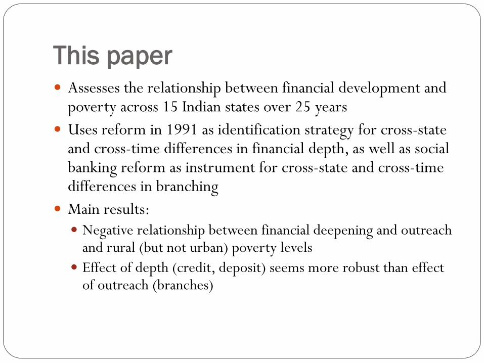
This paper Assesses the relationship between financial development and

poverty across 15 Indian states over 25 years

Uses reform in 1991 as identification strategy for cross-state and cross-time differences in financial depth, as well as social banking reform as instrument for cross-state and cross-time differences in branching

Main results:

Negative relationship between financial deepening and outreach and rural (but not urban) poverty levels

Effect of depth (credit, deposit) seems more robust than effect of outreach (branches)

Rural Poverty Pre and Post-Reform

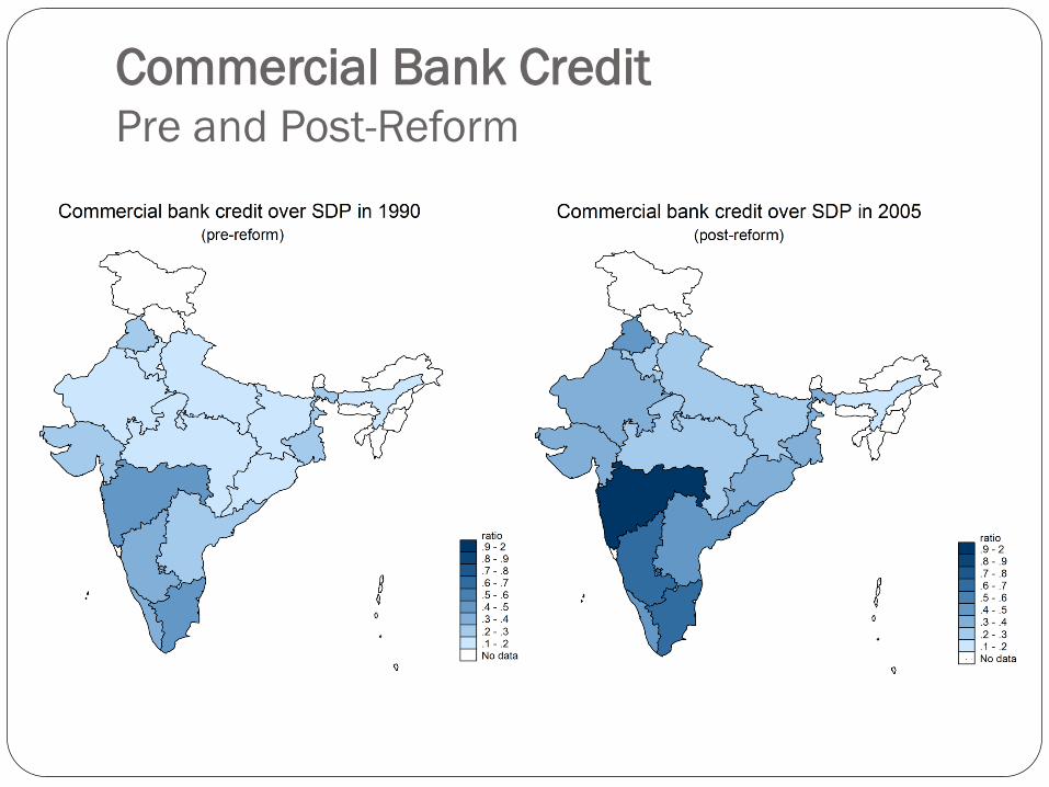
Commercial Bank Credit Pre and Post-Reform

Bank Branches

Pre and Post-Reform

number45 - 5040 - 4535 - 40

30 - 3525 - 3020 - 2515 - 209.999999 - 154.999999 - 9.9999990 - 4.999999

No data

(post-reform)

No. rural branches per mill. capita in 2005

number45 - 5040 - 4535 - 40

30 - 3525 - 3020 - 2515 - 209.999999 - 154.999999 - 9.9999990 - 4.999999

No data

(pre-reform)

No. rural branches per mill. capita in 1990

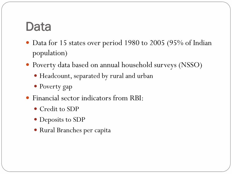
Data

Data for 15 states over period 1980 to 2005 (95% of Indian

population)

Poverty data based on annual household surveys (NSSO)

Headcount, separated by rural and urban

Poverty gap

Financial sector indicators from RBI:

Credit to SDP

Deposits to SDP

Rural Branches per capita

Methodology Annual data 1980-2005, differences in differences, i.e. state and

year-fixed effects

y(i, t) = (i) + (t) + FD(i,t) + C(i,t) + e(i,t) Y = rural/urban head count or poverty gap

State and year fixed effects

Errors clustered on state-level

Time-varying state-level control variables:

SDP per capita

Share rural population

Government expenditures/SDP

Literacy rate

Correlation table

Rural

Poverty

Credit/

SDP

Deposit

/SDP

Rural

Branches

(Mill.

Capita) SDP/Capita

Rural

population

Government

exp. /SDP

Credit/SDP -0.22**

Deposit/SDP -0.48** 0.72**

Rural Branches -0.25** -0.02 -0.02

SDP/Capita -0.74** 0.46** 0.63* 0.14**

Rural population 0.31** -0.78** -0.59** -0.23** -0.49**

Government exp. /SDP -0.08 -0.14** 0.07 -0.08 0.047 0.32**

Literacy rate -0.46** 0.52** 0.60** -0.09 0.53** -0.46** 0.16**

** Significant at 5% level

OLS – differences-in-differences (1) Rural Headcount

(1) (2) (3) (4) (5)

L.Bank Credit /SDP -23.366* -17.066**

(11.053) (7.905)

L.Bank Deposits /SDP -21.781* -24.555**

(11.611) (8.273)

L.Rural branches /mill.capita -1.302*** -1.215*** -1.348***

(0.351) (0.323) (0.331)

L.Log(SDP /capita) -0.677 -3.425 -2.167 -3.654 -8.097

(5.509) (6.072) (6.391) (6.002) (6.002)

L.rural population ratio -43.191 -30.607 62.309 28.026 32.510

(68.386) (73.470) (39.945) (46.202) (39.415)

L.literacy rate 0.112 0.013 0.021 0.039 -0.073

(0.197) (0.196) (0.222) (0.221) (0.210)

L.Government exp. / SDP 29.854 33.082 19.310 18.566 20.038

(24.278) (24.334) (19.114) (19.194) (19.650)

Constant 78.303 91.366 23.391 62.792 98.785

(57.725) (73.847) (57.083) (57.619) (57.532)

Observations 375 375 375 375 375

R-squared 0.909 0.908 0.918 0.920 0.922

Adjusted R-squared 0.897 0.896 0.907 0.910 0.912

# of States 15 15 15 15 15

Economic effects

One SD in credit: 3.5 pp reduction in rural headcount

One w/in SD in credit: 1.3 pp reduction in rural headcount

(26% o w/in variation)

One SD in rural branches: 9.5 pp reduction in rural

headcount

One w/in SD in credit: 2.1 pp reduction in rural headcount

(42% o w/in variation)

OLS – differences-in-differences (2) Rural Poverty Gap

(1) (2) (3) (4) (5)

L.Bank Credit /SDP -11.045** -8.921**

(4.469) (3.198)

L.Bank Deposits /SDP -10.293** -11.273**

(4.516) (3.888)

L.Rural branches /mill.capita -0.455** -0.410** -0.476**

(0.171) (0.161) (0.161)

L.Log(SDP /capita) 1.689 0.391 1.462 0.686 -1.260

(3.132) (3.247) (3.565) (3.476) (3.627)

L.rural population ratio -23.175 -17.222 18.761 0.839 5.080

(29.885) (33.890) (20.655) (23.204) (24.254)

L.literacy rate 0.069 0.023 0.035 0.045 -0.008

(0.095) (0.093) (0.114) (0.112) (0.106)

L.Government exp. / SDP 16.701 18.227* 13.283 12.894 13.617*

(9.702) (9.482) (7.737) (7.405) (7.237)

Constant 15.344 21.508 -10.483 10.114 24.129

(30.721) (36.673) (30.557) (32.506) (34.744)

Observations 375 375 375 375 375

R-squared 0.878 0.877 0.885 0.891 0.894

Adjusted R-squared 0.863 0.861 0.870 0.876 0.879

# of States 15 15 15 15 15

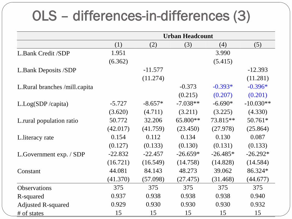
OLS – differences-in-differences (3)

Urban Headcount

(1) (2) (3) (4) (5)

L.Bank Credit /SDP 1.951 3.990

(6.362) (5.415)

L.Bank Deposits /SDP -11.577 -12.393

(11.274) (11.281)

L.Rural branches /mill.capita -0.373 -0.393* -0.396*

(0.215) (0.207) (0.201)

L.Log(SDP /capita) -5.727 -8.657* -7.038** -6.690* -10.030**

(3.620) (4.711) (3.211) (3.225) (4.330)

L.rural population ratio 50.772 32.206 65.800** 73.815** 50.761*

(42.017) (41.759) (23.450) (27.978) (25.864)

L.literacy rate 0.154 0.112 0.134 0.130 0.087

(0.127) (0.133) (0.130) (0.131) (0.133)

L.Government exp. / SDP -22.832 -22.457 -26.659* -26.485* -26.292*

(16.721) (16.549) (14.758) (14.828) (14.584)

Constant 44.081 84.143 48.273 39.062 86.324*

(41.370) (57.098) (27.475) (31.468) (44.677)

Observations 375 375 375 375 375

R-squared 0.937 0.938 0.938 0.938 0.940

Adjusted R-squared 0.929 0.930 0.930 0.930 0.932

# of states 15 15 15 15 15

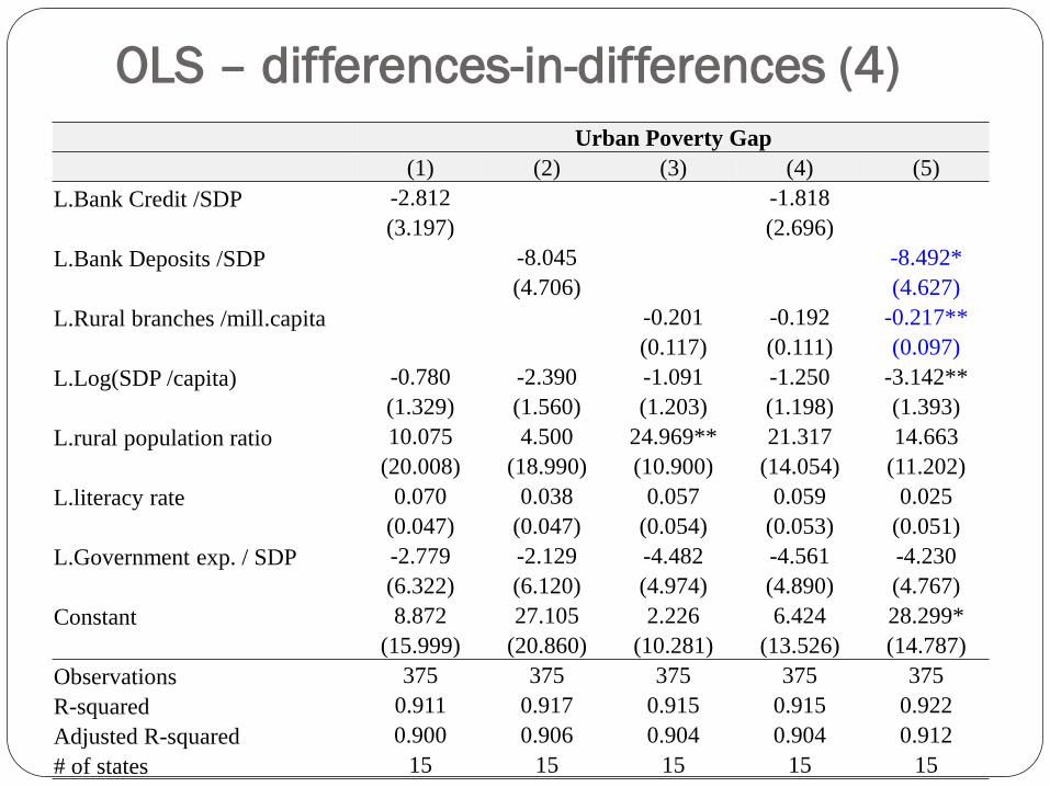
OLS – differences-in-differences (4)

Urban Poverty Gap

(1) (2) (3) (4) (5)

L.Bank Credit /SDP -2.812 -1.818

(3.197) (2.696)

L.Bank Deposits /SDP -8.045 -8.492*

(4.706) (4.627)

L.Rural branches /mill.capita -0.201 -0.192 -0.217**

(0.117) (0.111) (0.097)

L.Log(SDP /capita) -0.780 -2.390 -1.091 -1.250 -3.142**

(1.329) (1.560) (1.203) (1.198) (1.393)

L.rural population ratio 10.075 4.500 24.969** 21.317 14.663

(20.008) (18.990) (10.900) (14.054) (11.202)

L.literacy rate 0.070 0.038 0.057 0.059 0.025

(0.047) (0.047) (0.054) (0.053) (0.051)

L.Government exp. / SDP -2.779 -2.129 -4.482 -4.561 -4.230

(6.322) (6.120) (4.974) (4.890) (4.767)

Constant 8.872 27.105 2.226 6.424 28.299*

(15.999) (20.860) (10.281) (13.526) (14.787)

Observations 375 375 375 375 375

R-squared 0.911 0.917 0.915 0.915 0.922

Adjusted R-squared 0.900 0.906 0.904 0.904 0.912

# of states 15 15 15 15 15

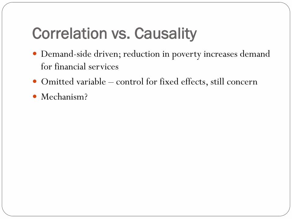
Correlation vs. Causality

Demand-side driven; reduction in poverty increases demand

for financial services

Omitted variable – control for fixed effects, still concern

Mechanism?

Looking for instruments Burgess and Pande: social branching experiment

4:1 rule between 1976 and 1990 for new branches led to increase in branches in previously unbanked areas

Three time trend* initial rural branch penetration

1991 liberalization – differential effects across different states Liberalization starting in 1991 led to more decentralized policy making, with

different states using their opportunities at reform to different extent Liberalization was broad, in the financial sector included interest rate

liberalization and reductions in reserve requirements, private bank entry etc. Reforms in areas of investment incentives, tax policy, power sector,

infrastructure etc. Bajpai and Sachs (1999) distinguish between three groups:

Reform-oriented: Andhra Pradesh, Gujarat, Karnataka, Kerala, Maharashtra and Tamil Nadu

Intermediate Reformers: Haryana, Orissa, Madhya Pradesh, Punjab, Rajasthan and West Bengal

Lagging Reformers: Assam, Bihar, and Uttar Pradesh

Three dummies – post 1991* reform category

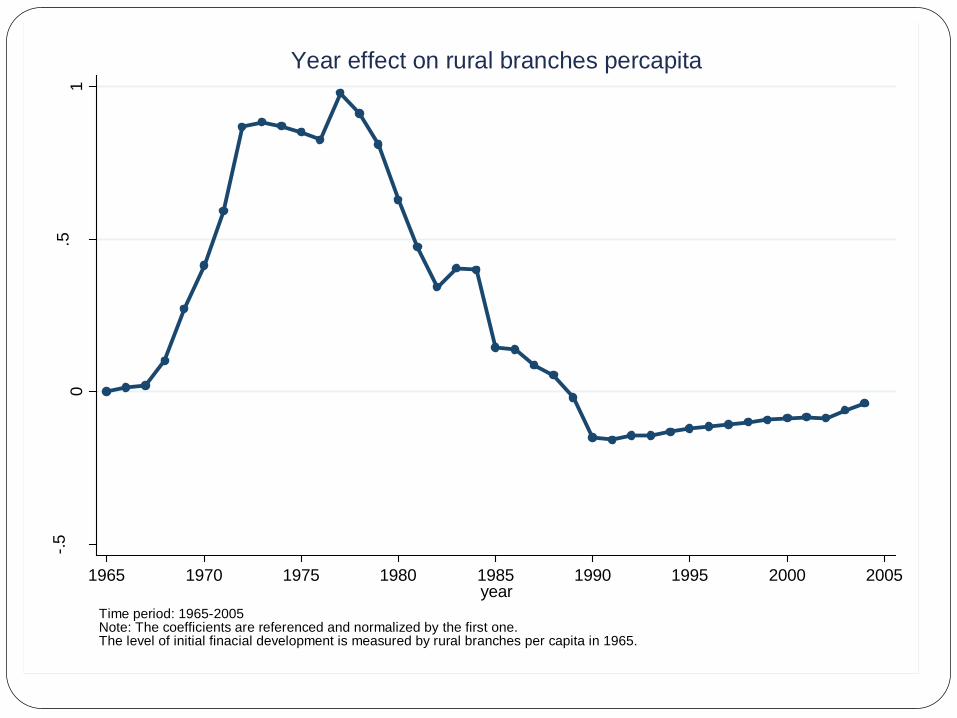
-.5

0.5

1

Initia

l financia

l develo

pm

ent x y

ear

1965 1970 1975 1980 1985 1990 1995 2000 2005year

Time period: 1965-2005Note: The coefficients are referenced and normalized by the first one.The level of initial finacial development is measured by rural branches per capita in 1965.

Year effect on rural branches percapita

0.2

.4.6

1970 1980 1990 2000 2010year

lagging-reformers intermediate-reformes reform-oriented

Credit_over_SDP

First stage regressions

L.Rural

branches /mill.capita

L.Bank Credit /SDP

L.Bank Deposits /SDP

(1) (2) (4)

L.Dummy for post 1991 x Lagging Reformers Dummy 17.961* 0.629** 1.231***

L.Dummy for post 1991 x Intermediate Reformers Dummy 17.922 0.661** 1.245***

L.Dummy for post 1991 x Reform Oriented Dummy 18.919 0.733* 1.331***

L.(year-1965) x Rural Branches in 1965 0.447*** 0.001 0.004***

L.(year-1977) x Rural Branches in 1965 x Dummy for post 1977 -0.606*** -0.001 -0.005***

L.(year-1990) x Rural Branches in 1965 x Dummy for post 1990 0.181* 0.000 0.004**

L.Log(SDP /capita) -3.280 -0.225* -0.368***

L.rural population ratio 51.580 -1.397** -0.854

L.literacy rate -0.058 0.000 -0.003

L.Government exp. / SDP -8.810 -0.024 0.158

Constant -2.477 2.895** 3.616***

Observations 375 375 375

R-squared 0.966 0.908 0.951

Adjusted R-squared 0.961 0.896 0.944

F_test 12.390 4.773 17.232

P_value 0.000 0.008 0.000

# of States 15 15 15

Standard errors not reported in above table

Second stage regressions

Rural

Headcount

Rural

poverty

gap

Urban

Head

count

Urban

poverty

gap

Rural

Headcount

Rural

poverty gap

Urban

Head

count

Urban

poverty

gap

1 2 3 4 5 6 7 8

L.Bank Credit /SDP -116.862* -44.974* -41.069 -22.899

L.Rural branches /mill.capita -2.274 -0.468 -0.937 -0.083 -2.248** -0.467 -0.741 -0.047

L.Bank Deposits /SDP -89.685*** -33.889*** -44.576 -19.729*

L.Log(SDP /capita) -17.011* -3.174 -12.92* -3.079 -26.140** -6.566 -18.649** -5.285**

L.rural population ratio -94.918 -59.625 21.542 -21.130 -8.102 -24.953 25.755 -8.459

L.literacy rate 0.056 0.069 0.134 0.081 -0.365 -0.091 -0.052 -0.008

L.Government exp. / SDP -1.093 8.961 -36.00** -5.460 14.379 14.798* -28.113* -2.024

Constant 291.92** 93.154* 142.460 55.097 298.128** 93.613* 184.909* 62.960

Observations 375 375 375 375 375 375 375 375

R-squared 0.826 0.794 0.911 0.870 0.887 0.858 0.928 0.906

Adjusted R-squared 0.803 0.766 0.899 0.852 0.872 0.839 0.919 0.893

Sargan 2.513 1.310 17.072 10.867 3.249 2.653 11.483 8.803

p_value 0.642 0.860 0.002 0.028 0.517 0.617 0.022 0.066

# of States 15 15 15 15 15 15 15 15

Standard errors not reported in above table

Conclusions

Negative relationship between financial development and

rural poverty across states and over time

New instruments: reform variation across states after 1991

liberalization

Instrumenting confirms results on financial depth (credit and

deposits)

Horse race shows more robustness for depth than for

outreach (branch penetration)