Finance and Economics Discussion SeriesDivisions of Research & Statistics and Monetary Affairs

Federal Reserve Board, Washington, D.C.

Commercial and Residential Land Prices Across the United States

Joseph B. Nichols, Stephen D. Oliner, and Michael R. Mulhall

2010-16

NOTE: Staff working papers in the Finance and Economics Discussion Series (FEDS) are preliminarymaterials circulated to stimulate discussion and critical comment. The analysis and conclusions set forthare those of the authors and do not indicate concurrence by other members of the research staff or theBoard of Governors. References in publications to the Finance and Economics Discussion Series (other thanacknowledgement) should be cleared with the author(s) to protect the tentative character of these papers.

Commercial and Residential Land Prices Across the United States

Joseph B. Nichols, Stephen D. Oliner, and Michael R. Mulhall* Federal Reserve Board

Revised: February 2010 Initial draft: May 2009

Abstract

We use a national dataset of land sales to construct land price indexes for 23 MSAs in the United States and for the aggregate of those MSAs. We construct the price indexes by estimating hedonic regressions with a large sample of land transactions dating back to the mid-1990s. The regressions feature a flexible method of controlling for spatial price patterns within an MSA. The resulting price indexes show a dramatic increase in both commercial and residential land prices over several years prior to their peak in 2006-07 and a steep descent since then. These fluctuations in land prices are considerably larger than those in well-known indexes of commercial real estate and house prices. Because those existing indexes price a bundle of land and structures, this comparison implies that land prices have been more volatile than structures prices over this period. *Contact author: Nichols, joseph.b.nichols@frb.gov, (202) 452-2983. We thank Christopher Reynolds for producing the location maps that we use in the paper. We received valuable comments from numerous Federal Reserve colleagues at an early stage of this study and from Edward Millner and other participants at the AREUEA 2009 mid-year meeting. We also thank Andreas Lehnert, Hui Shan, and Shane Sherlund for helpful conversations on estimation issues and Dan Sichel for useful comments on a recent draft of the paper. The data for this study were provided by the CoStar Group, Inc. The views expressed herein are those of the authors alone and should not be attributed to the Board of Governors of the Federal Reserve System or other members of its staff.

- 1 -

1. Introduction

All types of economic activity require land, either directly or indirectly. The direct use of

land is obvious in industries such as farming and construction. But all other forms of commerce

ultimately require land as well because workers, equipment, and buildings need to be located

somewhere. Even a cutting-edge high-tech company like Google has a corporate campus in

Silicon Valley and more than 65 other offices, research facilities, and data centers around the

world.1

The importance of land is reflected in available estimates of its aggregate value. A broad

measure of the value of residential and commercial land in the United States can be derived from

the Flow of Funds (FOF) accounts published by the Federal Reserve Board. The implied FOF

estimate – which covers land held by households, nonprofit organizations, and businesses other

than farms and financial corporations – equals the market value of real estate minus the

replacement cost of structures. At the end of 2009:Q3, this estimate of land value in the United

States was roughly $4½ trillion.2

With such a large aggregate value, changes in land prices can have a substantial effect on

the net worth of businesses and households. In this regard, Davis and Heathcote (2007) estimate

that swings in residential land prices accounted for most of the variation in house prices over

1975-2006 for the United States as a whole. Davis and Palumbo (2008) reach the same

conclusion for a large set of metropolitan areas over a somewhat shorter sample period, as do

1 See www.google.com/corporate/address.html for a listing of Google’s locations. 2 The data for this estimate are in tables B.100, B.102, and B.103 of the Flow of Funds Accounts of the United States, available at www.federalreserve.gov/release/z1. Barker (2007), Case (2007), and Davis (2009) present analogous estimates from earlier vintages of the Flow of Funds data. Note that all such estimates should be regarded as subject to considerable measurement error. The Flow of Funds accounts stopped publishing an explicit measure of land value in 1995, at least in part because of concerns about the accuracy of the estimates. Nonetheless, the discontinued series on land value can be reconstructed from other series published in the accounts. For other estimates of national land values that do not rely on Flow of Funds data, see Davis and Heathcote (2007), Barker (2007), and the Bureau of Labor Statistics (2007), along with the earlier work by Goldsmith (1951) and Manvel (1968).

- 2 -

Bostic, Longhofer, and Redfearn (2007) in their detailed analysis of home price changes within a

single metropolitan area (Wichita, Kansas).

Land also serves as a form of collateral for loans, especially for construction loans. If the

borrower defaults before a construction project is finished, the lender’s recovery will depend in

large part on the value of the land pledged as collateral. Commercial banks in the United States

have substantial exposure to land prices through their lending activities. At the end of 2009:Q3,

U.S. commercial banks held about $440 billion in construction and land development loans, and

more than 18 percent of these loans were delinquent – by far the highest delinquency rate among

the major types of bank loans.3

Despite the importance of land as a component of wealth, as a source of variation in real

estate prices, and as collateral for loans, only a handful of studies have calculated land price

indexes for the nation as a whole or for a broad set of cities.4 Davis and Heathcote (2007) and

Davis and Palumbo (2008) estimate price indexes for residential land, while Davis (2009)

estimates indexes for both residential and commercial land. These indexes, however, are not

based on transaction prices. Instead, Davis and his coauthors infer land prices as a residual from

data on real estate prices and construction costs, combined with the assumption that the prices of

existing structures always equal their replacement cost. This identifying assumption likely is

reasonable over long spans of time, but it may not be valid over shorter periods.5

3 These figures represent aggregates from the Consolidated Reports of Condition and Income (Call Reports) submitted by domestic commercial banks to the Federal Financial Institutions Examination Council. See Bech and Rice (2009) for an in-depth analysis of the Call Report data. 4 That said, there are numerous studies of land prices for single cities or other narrow geographic areas. See, for example, Brownstone and DeVany (1991), Colwell and Munneke (1997, 2003), Guntermann and Thomas (2005), Haughwout, Orr, and Bedoll (2008), Isakson (1997), Kowalski and Paraskevopoulos (1990), Peiser (1987), and Wieand and Muth (1972). These studies cover commercial land or a combination of commercial and residential land. For studies that focus exclusively on residential land, see Bryan and Sarte (2009), Downing (1970), Greenlees (1980), Ihlanfeldt (2007), Rosenthal and Helsley (1994), and Voith (2001). 5 Indeed, the standard neoclassical theory of investment with adjustment costs, as embodied in Tobin’s q, links the volume of investment spending to the size of the gap between the market value of an asset and its replacement cost.

- 3 -

In contrast, Sirmans and Slade (2009) use transaction prices to calculate national land

price indexes. However, they do not estimate price indexes for individual metropolitan statistical

areas (MSAs), an important limitation given the substantial local variation in real estate markets.

In addition, Sirmans and Slade use a very small set of variables to control for the dispersion in

land prices in their regressions, do not allow the effects of these variables on land prices to differ

across MSAs or property types, and do not weight the data to ensure that their price indexes are

nationally representative. Our study addresses all of these methodological issues and calculates

land price indexes not only at the national level but also for individual MSAs. We provide the

first transaction-based indexes of land prices for a broad swath of MSAs across the United

States.

Using source data obtained from the CoStar Group, Inc., we construct a dataset that

includes more than 170,000 land transactions in 23 MSAs.6 These MSAs include the major

population centers in the United States and some smaller cities. For most MSAs, the data span

the period from the mid- or late 1990s to the middle of 2009. We use these data to estimate a set

of hedonic equations for residential and commercial land prices.7 The explanatory variables in

the equations include a number of characteristics of the property and the sale transaction, a

flexible specification of the effects of location on price within an MSA, and half-yearly dummy

variables to capture the changes in land prices over time after controlling for the other factors.

The specification of locational effects combines the property’s distance from the central business

Davis and Heathcote (2007) and Davis and Palumbo (2008) assume, in effect, that this gap is always zero for residential structures, and Davis (2009) makes the same assumption for both residential and commercial structures. This assumption is valid only if the stock of these structures can be adjusted very rapidly in response to changes in economic conditions, which seems unlikely given the planning and construction lags inherent in real estate projects. 6 In addition to our paper and Sirmans and Slade (2009), other studies that have used the CoStar land-price data include Haughwout, Orr, and Bedoll (2008) for New York City and Colwell and Munneke (2003) for Chicago. 7 The commercial land sales in our dataset cover not only properties slated for office and retail development but also industrial sites. To avoid confusion about the types of land in our dataset, we will use the label “commercial/industrial” rather than “commercial” for the rest of the paper.

- 4 -

district, which has been used in many studies, and the semiparametric specification introduced in

Colwell (1998) that can accommodate a much wider range of spatial patterns.

Our primary focus is on the land price indexes implied by the coefficients on the half-

yearly dummy variables. For the 23 MSAs as an aggregate, we present price indexes for a

composite of residential and commercial/industrial land along with separate indexes for these

two broad types of land. We also report the analogous price indexes for each MSA in all periods

for which sufficient data are available.

The results show that land prices trended up at a moderate pace from 1995 until about

2002, and then accelerated sharply. From the second half of 2002 to the first half of 2007, our

composite index of residential and commercial/industrial land prices for the 23 MSAs jumped

nearly 130 percent, with even larger increases in the MSAs along the East Coast and in the Far

West. However, prices have tumbled over the past few years, leaving the composite index for

the 23 MSAs in the first half of 2009 more than 40 percent below its peak. These moves outstrip

the variation since 2002 in well-known national indexes of house prices and commercial real

estate prices. Because those indexes price a bundle of land and structures, this comparison

implies that land prices have been more volatile than prices of structures over this period. This

greater volatility confirms the findings in Davis and Heathcote (2007) and Davis and Palumbo

(2008) for residential property for an earlier period. Intuitively, land prices should be more

volatile than the prices of structures because the latter are tied, at least loosely, to construction

costs, while land prices have no such anchor.

The remainder of the paper is organized as follows. The next section describes our

dataset on land transactions. Section 3 presents our approach to modeling the effects of location

on land prices, and section 4 describes all other aspects of the empirical methodology. Section 5

- 5 -

presents the estimation results. The final section summarizes our conclusions and lays out the

next steps in this line of research.

2. Data

The data for our analysis were obtained from the CoStar Group, a major provider of

information on commercial real estate in the United States (www.costar.com). Among its

various data products, CoStar maintains a database on sales of commercial property and land in

the United States (the “COMPS” database). CoStar obtains the transaction data from public

records, interviews with parties to the transactions, and field inspection of the properties.

Currently, the COMPS database includes more than one million transactions.

We analyze the transactions in COMPS explicitly identified as land sales. CoStar defines

land sales as transactions that involve vacant property or property with unoccupied structures

that are slated for demolition. These criteria ensure that the value of any existing structures

should be incidental to the total value of the property. A separate field in COMPS indicates

whether the intended use of the land is residential, industrial, or commercial. To be included in

COMPS, a residential land parcel must consist of at least five single-family lots or be large

enough to support multifamily buildings with at least five units. There is no lower size limit in

COMPS for the value of included land sales. However, only seven percent of our sample

consists of sales of $250,000 or less.

Each transaction record contains the sales price, address, and the longitude and latitude of

the land parcel, along with a series of text fields describing the characteristics of the parcel. We

use the information in these text fields to create a number of indicator variables for our hedonic

price regression. The indicators include various improvements to the raw land (whether it has

been paved, graded, finished, fully improved, previously developed, or platted); other

- 6 -

characteristics of the property (the presence of existing structures and the presence of soil or

building contamination); the proposed final use of the land (private development, public use,

open space, or land to be held for investment); and characteristics of the transaction itself

(whether it is a foreclosure sale, an acquisition through eminent domain, or an expansion of a

neighboring property).

For the analysis in this paper, we constructed a dataset with more than 170,000 land

transactions in 23 MSAs.8 These MSAs include five cities in the Northeast corridor (Boston,

New York, Philadelphia, Baltimore, and Washington DC); three areas in Florida (Orlando,

Tampa/St. Petersburg, and South Florida); six cities on the West Coast (Los Angeles, San Diego,

San Francisco, Sacramento, Seattle, and Portland); and nine cities in the interior of the country

(Atlanta, Chicago, Dallas, Denver, Detroit, Houston, Las Vegas, Phoenix, and Tucson). Prior to

1995, the transaction data for most of these MSAs is either sparse or nonexistent. Accordingly,

we standardized the starting point of the analysis in 1995, except for six MSAs for which the

data begin between 1997 and 1999. The transaction data are available through the first half of

2009.

Table 1 provides information on the sample for each MSA and for the 23 MSAs taken

together. As shown, of the roughly 172,000 sales transactions, about 95,000 (or 55 percent)

involve commercial or industrial land, while the other 77,000 represent sales of land intended for

8 Our complete database includes roughly 250,000 transactions in 138 MSAs. However, many of these MSAs have relatively few observations, and we restrict our attention to the MSAs with the richest data. For the 23 MSAs covered by our analysis, we excluded almost five percent of the land sales that we downloaded from COMPS, either because of missing data for the explanatory variables, because the land parcel was geographically isolated from other observations in its MSA, or because we judged the number of observations for an MSA in a given half-year to be insufficient to generate a reliable price index for that period. We settled on minimum half-yearly sample sizes after observing the volatility in the price indexes generated without regard to sample size. Based on these results, we included the residential or commercial/industrial transactions for an MSA in a given half-year only when we had more than 30 observations for that property type. For regressions in which we estimated a single MSA-level price index that covered both property types, we included a given half-year only when we had more than 40 observations in total.

- 7 -

residential projects. The sample sizes for the individual MSAs vary widely, ranging from about

2,400 for Houston to more than 17,000 for Phoenix. This variation reflects, at least in part,

differences in the amount of development activity across the MSAs and does not correlate

closely with the relative shares of the MSAs in national stocks of residential or

commercial/industrial land. Because of this disconnect, we employ MSA-level weights,

described in section 4, to obtain nationally representative results.

The other key dimension of the sample is the number of observations over time. Figure 1

shows one measure of this time pattern – the median sample size across the 23 MSAs for each

half-year since 1995; the figure presents separate series for commercial/industrial and residential

transactions.9 As shown by the dashed line, the median MSA has at least 80 residential land

transactions in every half-year through the first half of 2006, and more than 100 transactions in

most of these periods. However, transaction volume plunged after mid-2006 with the collapse in

housing activity. For commercial/industrial land, transaction volume was well maintained

through 2007 but dropped sharply in 2008 and the first half of 2009. Given the sample-size

cutoffs described above, these patterns imply that we have insufficient data to calculate land

price indexes for some MSAs in recent years, though we are able to calculate indexes through

2009:H1 for the 23 MSAs taken together.

3. Locational Effects on Land Prices

The location of a property is a prime determinant of its value. Home values reflect the

proximity to good schools, employment opportunities, recreation, and transportation, along with

the amount of crime in local neighborhoods and the quality of services provided by local

9 We show the median sample size across MSAs for each period, rather than the average sample size or the total number of observations, to reduce the distorting effect from the increase in the number of MSAs in the sample from 1995 to 1999. Note also that the figure presents the median sample size across MSAs before applying the cutoff rules described in the previous footnote. We do this to display the underlying time patterns in transaction volume.

- 8 -

government. Similarly, the value of commercial property varies with its proximity to

transportation hubs and arteries, the presence of complementary business activities (such as retail

stores interspersed with restaurants), and the income level and other demographics of the local

population. These locational effects would be expected to be even stronger for undeveloped land

than for existing residential or commercial real estate, as the market value of the buildings at

those sites would be tied – at least loosely – to the construction costs for the metropolitan area as

a whole. Land values have no such anchor and are driven by the anticipated profit of developing

a specific site.

Given the likelihood of important locational effects, empirical studies of land prices have

included one or more variables to capture these effects. A simple and very common

specification uses the property’s distance from the central business district (CBD) of its MSA as

a primary measure of its location.10 This specification, however, imposes strong restrictions on

locational effects. Consider two properties located at different points on a circle centered at the

CBD. If the two properties are identical apart from their location on the circle, this specification

implies that they will have the same market value, regardless of differences in their proximity to

various amenities. Recognizing that distance from the CBD is unlikely to fully capture

locational effects, most studies have included other variables as well. The added variables have

included the distance from major roads, rail lines, and airports; distance from suburban business

nodes; distance from the coastline; dummy variables for local topography; dummy variables for

location within the city limits and within specific counties; measures of the amount of street

frontage; and demographic information for the surrounding area.

10 See, for example, Brownstone and DeVany (1991), Colwell and Munneke (1997), and Peiser (1987). In a similar specification for the New York City area, Haughwout, Orr, and Bedoll (2008) use the property’s distance from the Empire State Building.

- 9 -

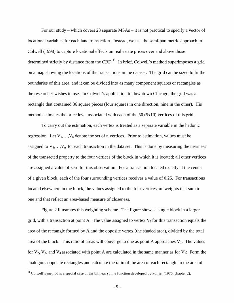
For our study – which covers 23 separate MSAs – it is not practical to specify a vector of

locational variables for each land transaction. Instead, we use the semi-parametric approach in

Colwell (1998) to capture locational effects on real estate prices over and above those

determined strictly by distance from the CBD.11 In brief, Colwell’s method superimposes a grid

on a map showing the locations of the transactions in the dataset. The grid can be sized to fit the

boundaries of this area, and it can be divided into as many component squares or rectangles as

the researcher wishes to use. In Colwell’s application to downtown Chicago, the grid was a

rectangle that contained 36 square pieces (four squares in one direction, nine in the other). His

method estimates the price level associated with each of the 50 (5x10) vertices of this grid.

To carry out the estimation, each vertex is treated as a separate variable in the hedonic

regression. Let V1,…,Vn denote the set of n vertices. Prior to estimation, values must be

assigned to V1,…,Vn for each transaction in the data set. This is done by measuring the nearness

of the transacted property to the four vertices of the block in which it is located; all other vertices

are assigned a value of zero for this observation. For a transaction located exactly at the center

of a given block, each of the four surrounding vertices receives a value of 0.25. For transactions

located elsewhere in the block, the values assigned to the four vertices are weights that sum to

one and that reflect an area-based measure of closeness.

Figure 2 illustrates this weighting scheme. The figure shows a single block in a larger

grid, with a transaction at point A. The value assigned to vertex V1 for this transaction equals the

area of the rectangle formed by A and the opposite vertex (the shaded area), divided by the total

area of the block. This ratio of areas will converge to one as point A approaches V1. The values

for V2, V3, and V4 associated with point A are calculated in the same manner as for V1: Form the

analogous opposite rectangles and calculate the ratio of the area of each rectangle to the area of 11 Colwell’s method is a special case of the bilinear spline function developed by Poirier (1976, chapter 2).

- 10 -

the block. All other vertices in the grid surrounding this block have a value of zero for the

transaction represented by point A.

After the values for V1,…,Vn have been assigned in this manner for each transaction in

the dataset, a hedonic price regression can be estimated with the vertices included as explanatory

variables.12 The estimated coefficient for a given vertex represents the height of the price surface

at that point on the grid. Colwell shows that the surface defined by these estimated grid points is

continuous, piecewise linear along the edges of the individual blocks, and parabolic along slices

within each block.

In implementing this method, we laid out the grids for the individual MSAs to conform to

the spatial pattern of the land transactions. For five of the MSAs (Atlanta, Dallas, Denver, Las

Vegas, and Tucson), we were able to encompass the vast majority of transactions with a

rectangular 5x5 grid composed of individual rectangular blocks. With a 5x5 grid, we estimate

coefficients for 36 vertices (6x6) on the spatial price surface. As an example, figure 3 shows the

5x5 grid for Dallas, superimposed on a scatter plot of the transactions in our dataset. For the

other MSAs, the spatial distribution of transactions did not fit well within a rectangular outline –

generally because of the presence of a body of water or mountains – and we drew the outline of

the grid to fit these patterns. In each case, the grid consists of between 22 and 28 individual

blocks (with between 36 and 42 vertices), arranged in a non-rectangular shape. As an

illustration, figure 4 presents the grid used for South Florida, where the land transactions occupy

a band that parallels the coastline.

In summary, we take a hybrid approach to modeling locational effects on land prices.

We include distance from the CBD as an explanatory variable in the regressions, which we

12 If the regression includes a constant term, one vertex must be omitted to avoid perfect colinearity among the explanatory variables. The colinearity arises because the vertex weights for any observation sum to one.

- 11 -

augment with the semi-parametric grid method described above to capture the features of the

spatial price surface that do not lie on a constant gradient away from the CBD.

4. Specification and Estimation of the Hedonic Price Equation

We use the data described in section 2 to estimate a flexible hedonic regression for land

prices. The dependent variable in the regression is the natural log of the price of land per square

foot. The explanatory variables can be broken into three broad categories: property and

transaction characteristics other than location (X1 ,…, XJ), measures of location (Z1 ,…, ZK), and a

set of half-yearly time dummies (D1 ,…, DT). The regression pools the data for all 23 MSAs, but

it allows the coefficient on each explanatory variable to differ both across MSAs and across the

residential and commercial/industrial land transactions within an MSA. In effect, the pooled

regression stacks 46 separate regressions (23 MSAs with two broad types of land in each MSA)

and provides a convenient framework for testing a wide range of coefficient restrictions across

the MSAs and property types. Each regression in the stack can be written as

(1) , , , , , , , ,ln m l m l j j m l k k m l t t m lj k tP X Z D

where ,m lP is the vector of observations of price per square foot in the mth MSA for the lth broad

land type (l equals either residential or commercial/industrial), and ,m l is the corresponding

vector of errors. The subscripts on the , , and coefficients show that these coefficients are

allowed to vary across MSAs and property types.

The vector of property and transaction characteristics (X1 ,…, XJ) includes the natural log

of the size of the parcel in order to test the so-called “plattage effect”. Plattage refers to the

common empirical finding that the price of a land parcel rises less than proportionally with its

size. This relationship likely arises because there is an optimal scale for buildings of a given

- 12 -

type, which implies that parcels larger than the size needed to support the optimal building scale

earn a lower return.

The other variables in X1 ,…, XJ are the indicator variables mentioned in section 2. These

variables, which are largely the same as those used by Haughwout, Orr, and Bedoll (2008),

include:

Type of property: two sets of dummy variables, one for residential land and another for

commercial/industrial land. The residential set includes separate dummies for land used for

single-family housing and for multifamily rental projects, with condominiums as the omitted

land use. The commercial/industrial set includes dummies for industrial sites and for

commercial development other than office buildings, with office development as the omitted

category.

Condition of the property: separate dummy variables for whether the land has been graded,

paved, finished, fully improved, platted and engineered, or previously developed; whether it

has an existing structure; or whether the improvements are reported as unknown. The

omitted condition is unimproved land. This group of variables also includes a dummy for

whether environment problems exist as defined by reported soil or building contamination.

Intended use of the property: separate dummy variables for property intended for public use,

to be kept as open space, to be held for investment, or with an unknown use. The omitted

category is private development.

Characteristics of the transaction: separate dummy variables for property sold in foreclosure,

taken in an eminent domain proceeding, or purchased as part of the buyer’s plan to expand a

neighboring property.

- 13 -

The vector of location characteristics (Z1 ,…, ZK) includes the MSA-specific sets of grid

vertices described in the previous section, which provide a flexible way to control for the spatial

price patterns within an MSA. We specify a separate grid for residential land and

commercial/industrial land in each MSA. In addition to these grid vertices, we include the

natural log of distance of each property from the population-weighted center of its MSA. The

coefficient on this distance measure is allowed to vary by MSA and by broad property type,

consistent with the treatment of other variables in the regression. Finally, we include a set of

MSA fixed effects, with New York City as the omitted MSA.

We weight the observations in the regression prior to estimation. Weighting is required

because, as discussed in section 2, the number of land sales by MSA in our dataset does not

reflect the relative shares of the MSAs in national stocks of commercial/industrial and residential

land. To illustrate how we correct for this divergence, assume that a particular MSA accounts

for 20 percent of the residential land sales in the dataset but for only five percent of total

residential land in the 23 included MSAs. The dataset, therefore, overweights this MSA’s

residential land sales by a factor of four. As a correction, we would apply a weight of 0.25 to

each residential land sale from this MSA. A weight for commercial/industrial land can be

defined in the same manner; generally, this weight will differ from the weight for the MSA’s

residential land. Ideally, we would construct weights based on information on the available land

area devoted to commercial/industrial and residential real estate by MSA. In the absence of such

land data, we weighted the commercial/industrial land observations using estimates from Torto

Wheaton Research of the total space in commercial and industrial buildings by MSA and the

residential land observations using the number of occupied single-family and multifamily

- 14 -

housing units from the 2000 Census. We re-adjust these weights on a period-by-period basis to

account for the exclusion of MSAs with insufficient observations during particular time periods.

The pooled regression is estimated by maximum likelihood with a variance-covariance

matrix (Σ) that allows the variance of the error term to differ by MSA. Specifically, we assume

that Σ is diagonal, with 2m (m = 1,…,23) as the error variance for every observation in the mth

MSA. This structure accommodates potential differences across MSAs in the amount of

unobserved heterogeneity in land parcels and in the size of the shocks hitting the MSAs.

Our dataset consists of land sold over a given period and is not a random sample of land

parcels, which raises the possibility of sample selection bias. However, the traditional Heckman

(1979) procedure to correct for selection bias is not feasible in our case. To implement this

procedure, we would need data on vacant land parcels that were not sold during the sample

period. Such data would be very difficult to assemble for a large number of MSAs.13 Moreover,

it is unclear whether any such effort would be worthwhile. The results of studies that have

applied the Heckman procedure to real estate prices have been mixed to date. Although there is

some evidence of selection bias in house prices (see, for example, Gatzlaff and Haurin

(1997,1998) and Jud and Seaks (1994)), the few available studies for commercial real estate and

land prices have found that selection effects were generally small and insignificant.14

5. Results

This section presents the results from the estimation of the hedonic price function in

equation 1. We discuss the results in three steps, focusing first on the estimated coefficients for

13 Strictly speaking, data also would be required for previously-developed properties that are candidates for redevelopment because our dataset include properties with structures that are slated for demolition. Obtaining data for unsold properties that meet this criterion would be even more difficult than collecting data on unsold vacant land. 14 See Colwell and Munneke (1997) for an analysis of selection effects for commercial and residential land prices and Fisher, Geltner, and Pollakowski (2007) and Munneke and Slade (2000, 2001) for analyses of selection effects for commercial real estate prices.

- 15 -

the characteristics of the land parcels and the transactions, then on the spatial price effects, and

finally on the estimated variation in land prices over time.

Property and transaction characteristics

Table 2 summarizes the estimated coefficients for property and transaction characteristics

across the 23 MSAs for residential and commercial/industrial land. Each row reports the median

and range of coefficient values across the MSAs, along with the number of MSAs for which the

coefficients were either negative and significant or positive and significant at the five-percent

level.

Starting in the first row, the coefficient on the log of parcel size is strongly significant in

all 23 MSAs for commercial/industrial land and in all but two MSAs for residential land. The

median value of -0.53 for commercial/industrial land indicates that doubling the size of a parcel

reduces price per square foot by 53 percent. An equivalent statement is that doubling parcel size

boosts the total price of the parcel by only 47 percent. The median result for residential land is

essentially the same. These results confirm the plattage effect – that the price of a land parcel

rises less than one-for-one with its size.

The next block of the table shows the differences in price per square foot across the

different types of residential land and commercial/industrial land. For residential land, the price

difference between single-family properties and land used for condominiums (the omitted

category) spans a wide range across MSAs and is not consistently negative or positive. The

same is true for the comparison of multifamily properties and condominiums. In contrast, the

results show that industrial land sells at a discount to land for office development (the omitted

category), with a significant negative effect in 21 of the 23 MSAs. This discount likely arises

because the market-driven distribution of land use in a metropolitan area tends to push

- 16 -

warehousing and manufacturing activities to areas that are removed from amenities that enhance

property values. In the median MSA, land for non-office commercial development sells for less

than office property, but this result is not as consistent across MSAs as the discount for industrial

land.

Most of the indicators of the condition of a property have the expected effects on price.

Considering both residential and commercial/industrial land, property that has been graded,

finished, fully improved, or previously developed sells at an average price that is 11 to 33

percent above that for unimproved land in the median MSA; these price differentials are each

statistically significant for half or more of the 23 MSAs. The other property characteristics have

less consistently significant effects across the MSAs, though land that has been paved or platted

and engineered tends to sell, as expected, for more than unimproved land. One unanticipated

result for commercial/industrial land is the tendency for properties with missing information

about land improvements to sell at a discount to unimproved land. This result probably reflects

correlations with omitted variables that affect prices more for commercial/industrial land than for

residential land.

Among the other variables shown in table 2, land that is intended to be held for

investment, kept as open space, or has an unknown use sells for less than land purchased for

private development, as expected. These results are largely consistent across the two broad

property types. In contrast, with only a few exceptions, the price of land purchased for public

use is not significantly different than that for land purchased for private development. Variables

related to the sale transaction itself, shown in the final block of the table, seldom have a

significant effect on price, with the exception of commercial/industrial land purchased to

facilitate an expansion plan for the buyer. These properties tend to have a lower price in roughly

- 17 -

half of the MSAs than otherwise identical property for reasons that may reflect unobserved

features of such transactions.

The results in table 2 indicate that the coefficient estimates for a given variable can span a

wide range across MSAs and property types. We conducted an extensive set of hypothesis tests

to determine if these observed differences are statistically significant. The details of the tests can

be found in the appendix. However, the results can be summarized quite briefly. For the

variables shown in table 2, the tests overwhelmingly reject the null hypothesis that the

coefficients for residential land equal those for commercial/industrial land within the MSAs.

They also strongly reject the null hypothesis that the coefficients for residential land are the same

across all MSAs; the same result holds for commercial/industrial land. These results imply that

the property types and MSAs should not be aggregated when estimating the price effects of the

variables shown in table 2.

Locational effects

As discussed above, our regression equation features a hybrid specification of the

locational effects on land prices. For each MSA in the regression, we estimate separate

locational grids for residential land and commercial/industrial land, along with a distance

gradient from the CBD for each type of property. Taking all 23 MSAs together, the regression

includes more than 1,800 locational variables (23 measures of distance from the CBD and

roughly 900 grid vertices for each of the two property types).

The distance gradient is negative and significant (at the five-percent level) for residential

land in 17 MSAs and for commercial/industrial land in 15 MSAs; there are no instances of a

significant positive gradient. The median value of the gradient coefficient across MSAs is -0.35

for residential land and -0.30 for commercial/industrial land, so that doubling the distance from

- 18 -

the CBD reduces land value by roughly one-third, all else equal, in the median MSA. Overall,

these results show that a linear price gradient from the CBD is an important feature of land prices

in U.S. metropolitan areas.

However, distance from the CBD does not fully characterize the locational effects, as

indicated by the significant coefficients on many grid vertices. In 17 of the 23 MSAs, at least ten

of the grid vertices for residential land are statistically significant at the five-percent level; the

same result holds for commercial/industrial land in 15 MSAs. Evidently, the classic model of a

monocentric city with a linearly declining price gradient generally does not fit the MSAs in our

sample. This model may break down for any number of reasons, including the existence of

transportation corridors and satellite commercial hubs, differences in the quality of services

provided by different localities in the MSA, and the influence of topography and coast lines.

Figure 5 illustrates the latter effect with the estimated grids for residential land and

commercial/industrial land in South Florida. The back edge of the figure lies along the Atlantic

coast, with the highest part of the contour representing Miami Beach. The figure clearly shows a

price premium for land near the coast after controlling for distance from the CBD.

In sum, both elements of our hybrid approach are needed to model the spatial patterns of

land prices. Distance from the CBD is an essential determinant of prices, but there are other

features of the price surface that can only be captured with a more flexible specification.

Price indexes Given our controls for spatial price effects and for the heterogeneous features of the land

parcels and the sales transactions, the coefficients on the half-yearly dummy variables trace out

time-series indexes of land prices. These price indexes are the most important results in the

paper.

- 19 -

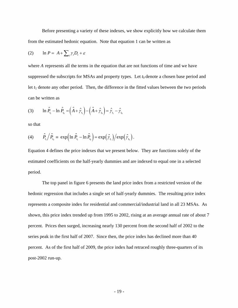
Before presenting a variety of these indexes, we show explicitly how we calculate them

from the estimated hedonic equation. Note that equation 1 can be written as

(2) ln t ttP A D

where A represents all the terms in the equation that are not functions of time and we have

suppressed the subscripts for MSAs and property types. Let t0 denote a chosen base period and

let t1 denote any other period. Then, the difference in the fitted values between the two periods

can be written as

(3) 1 0 1 0 1 0

ˆ ˆˆ ˆ ˆ ˆ ˆ ˆln lnt t t t t tP P A A

so that

(4) 1 0 1 0 1 0

ˆ ˆ ˆ ˆ ˆ ˆexp ln ln exp expt t t t t tP P P P .

Equation 4 defines the price indexes that we present below. They are functions solely of the

estimated coefficients on the half-yearly dummies and are indexed to equal one in a selected

period.

The top panel in figure 6 presents the land price index from a restricted version of the

hedonic regression that includes a single set of half-yearly dummies. The resulting price index

represents a composite index for residential and commercial/industrial land in all 23 MSAs. As

shown, this price index trended up from 1995 to 2002, rising at an average annual rate of about 7

percent. Prices then surged, increasing nearly 130 percent from the second half of 2002 to the

series peak in the first half of 2007. Since then, the price index has declined more than 40

percent. As of the first half of 2009, the price index had retraced roughly three-quarters of its

post-2002 run-up.

- 20 -

The lower panel shows separate price indexes for commercial/industrial and residential

land. To obtain these indexes, we re-estimated the regression using two sets of time dummies,

one for commercial/industrial land in all MSAs and another for residential land in all MSAs.

Both indexes display the same broad patterns as the composite index in the upper panel – a

moderate uptrend through 2002, followed by a sharp acceleration that lasted through 2006 or

2007 and then a steep reversal. However, the index for residential land displays greater

amplitude than either the composite index or the index for commercial/industrial land. A

likelihood ratio test decisively rejects the hypothesis that the residential and the

commercial/industrial price indexes are equal.

The basic features of the land price indexes estimated by Sirmans and Slade (2009) are

similar to those in figure 6. In particular, both sets of indexes indicate that land prices surged at

the national level after 2002 and have fallen sharply in recent years. There are, however, some

notable differences in the indexes. The total increase in the Sirmans-Slade indexes from 2002 to

the peak, while substantial, is not as large as in our indexes, and their indexes peak earlier than

ours. In particular, their composite index of commercial, industrial, and residential land prices

peaked in late 2005, when real estate markets were still booming, which seems less plausible

than the early 2007 peak in our composite index.

Figure 7 presents our land price indexes for the individual MSAs. These price indexes

cover an aggregate of commercial/industrial and residential land in the MSA and are calculated

using MSA-specific time dummies in the regression. The upper row of the figure shows the

indexes for MSAs on the East Coast while the middle row presents the indexes for West Coast

MSAs and the bottom row shows the indexes for MSAs located in the interior of the country.

All the series are indexed to equal 100 in 2002:H2 and every panel has the same scale, so the

- 21 -

magnitude of the post-2002 run-up in land prices and the subsequent decline can be compared

across MSAs.

The most striking feature of figure 7 is that the swing in land prices has been much larger

on the coasts and in Nevada and Arizona than elsewhere in the country, a pattern that mirrors the

boom-bust cycle in the housing market in recent years. In some MSAs – notably, Los Angeles,

Phoenix, Seattle, and South Florida – land prices have unwound most or all of the price spike,

while prices in other MSAs – including New York, Washington D.C., and Tampa – had reversed

only about half of the price spike by the first half of 2009.15 Land prices in Atlanta, Chicago,

Detroit, and Houston (the lower middle and right panels) have experienced a muted version of

this cycle, while the post-2002 price movements in Dallas and Denver are not easy to distinguish

from the underlying volatility in those series.

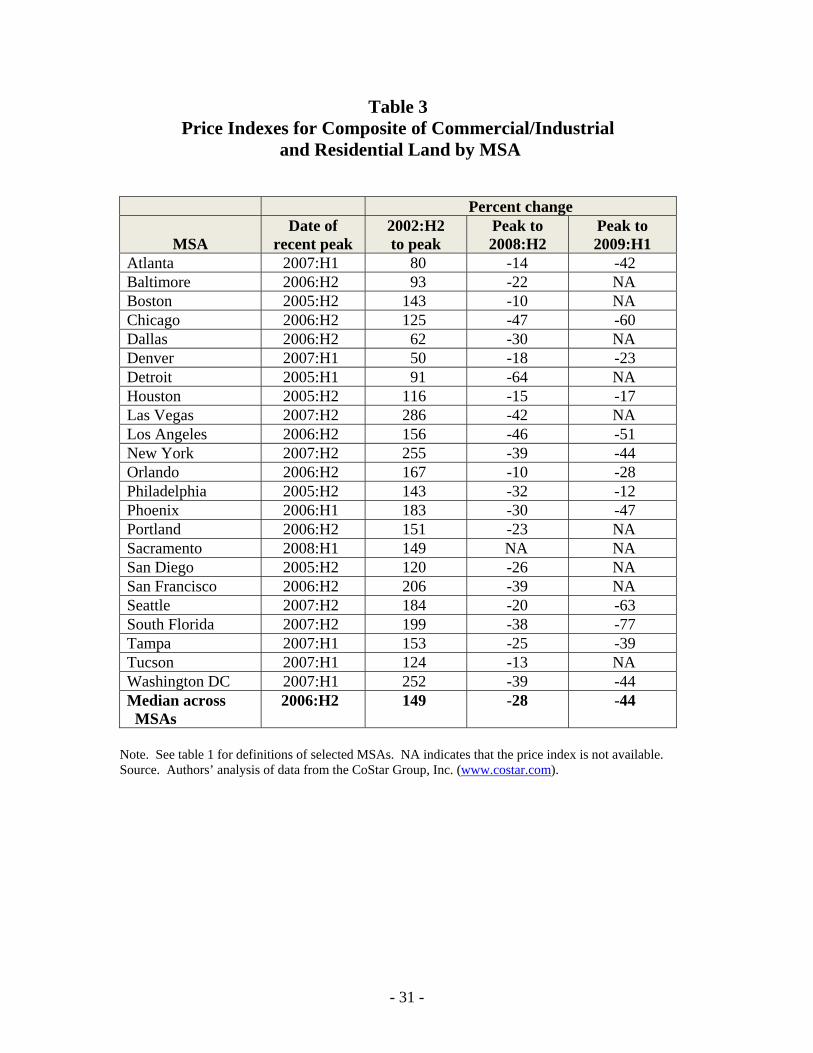
Table 3 provides additional information on the MSA-level land price indexes. As shown,

the price indexes for most MSAs reached a peak in 2006 or 2007, with the median peak date

across the MSAs occurring in the second half of 2006. The total price increase from the second

half of 2002 to the peak ranged from a low of 50 percent in Denver and 62 percent in Dallas to

more than 250 percent in Las Vegas, New York, and Washington DC; the median rise across

MSAs was 149 percent. Although the range is extremely wide, even the increases at the low end

of the range are not small in any absolute sense. More recently, all of the MSAs have

experienced sizable land-price declines from their respective peaks. As of the second half of

2008, the cumulative decline ranged from 10 percent in Boston and Orlando to 64 percent in

Detroit, with a median price drop of 28 percent across the MSAs. Adding in the first half of

15 For some MSAs, we were unable to calculate price indexes beyond the first half or second half of 2008 because the more recent transaction data were too sparse. For these MSAs – which include Baltimore, Boston, Dallas, Detroit, Las Vegas, Tucson, and all the West Coast cities except Los Angeles and Seattle – figure 7 may understate the full extent of the price decline through mid-2009.

- 22 -

2009 boosts the median decline to 44 percent for the 13 MSAs for which we have sufficient

transaction data. We should note, however, that the standard errors for the 2009:H1 dummy

variables for these MSAs are larger than for earlier periods because of the limited volume of land

sales.

Figure 8 and table 4 provide analogous results for the price indexes for

commercial/industrial land by MSA. These series, and the residential price indexes discussed

below, are calculated from the unrestricted version of the regression equation that allows the

coefficients of the half-yearly dummies to vary across both MSAs and property type. The MSA-

level movements in commercial/industrial land prices shown in figure 8 are qualitatively similar

to those displayed in figure 7 for the aggregate land price indexes. Both figures show that the

swings in commercial/industrial land prices generally have been wider in the MSAs on the East

Coast and in the Far West than elsewhere in the country. At the same time, a comparison of

tables 3 and 4 reveals some differences in specifics between the aggregate indexes and the

commercial/industrial indexes. The peak in commercial/industrial land prices occurred in the

first half of 2007 for the median MSA, one-half year after the peak in aggregate land prices. In

addition, in most MSAs the magnitude of the swing in the commercial/industrial series was not

quite as large as that for the aggregate series. For the median MSA, commercial/industrial land

prices rose 128 percent from 2002:H2 to the peak, about 20 percentage points less than the

median rise for aggregate land prices. Similarly, the median price decline from the peak to

2009:H1 was 39 percent, compared with a median drop of 44 percent for the aggregate series.

Finally, figure 9 and table 5 present the MSA-level results for the residential price

indexes. For most MSAs, prices jumped even more sharply for residential land than for

commercial/industrial land. Taking the median across MSAs, residential land prices increased

- 23 -

195 percent from the second half of 2002 to the peak, compared with the 128 percent rise for

commercial/industrial land prices. In addition, prices generally peaked earlier for residential

land than for commercial/industrial land. For the median MSA, residential land prices peaked in

the second half of 2006, a half-year before the peak in the commercial/industrial price series.

The steep decline in transaction volume since 2006 limits the number of MSAs for which we can

estimate the recent behavior of residential land prices. Nonetheless, the MSAs with sufficient

data have experienced a sharp drop in land prices. In the eight MSAs with data through

2008:H2, the median decline from the peak was 34 percent, and in the four MSAs with data all

the way through 2009:H1, the median decline ballooned to 59 percent.

An important issue is how these movements in land prices compare with the price

changes for housing and commercial/industrial real estate over the same period. In their

assessments of this issue, Davis and Heathcote (2007), Davis and Palumbo (2008), and Sirmans

and Slade (2009) found that the price swings for residential land have been wider than those for

home prices over various periods. Sirmans and Slade (2009) obtained the same result when

comparing their price index for industrial land to standard price indexes for industrial real

estate.16

Table 6 compares the land price indexes estimated in this study to well-known indexes of

commercial real estate and house prices. The land price indexes are the aggregate indexes for

commercial/industrial and residential land that were plotted in the lower panel of figure 6. We

compare the index of commercial/industrial land prices to two indexes of commercial real estate

prices: the National Council of Real Estate Investment Fiduciaries (NCREIF) transaction-based

16 However, their comparison of relative price movements for the non-industrial part of the commercial sector was inconclusive because of differences in the sectoral coverage of the indexes.

- 24 -

index and the Moody’s/REAL commercial property price index.17 In addition, we compare the

index of residential land prices to the S&P/Case-Shiller 20-city index of home prices.

As shown in the table, the price indexes for commercial/industrial land and commercial

real estate all peaked in 2007. However, commercial/industrial land prices rose substantially

more from the second half of 2002 to the peak than did either of the measures of commercial real

estate prices. Because the NCREIF and Moody’s/REAL indexes price a bundle of land and

structures, this comparison implies that commercial/industrial land prices increased more than

the prices of such structures. Qualitatively, the same pattern holds for the price declines since

the peak. In the residential sector, the excess amplitude in land prices relative to home prices has

been even starker. Residential land prices are estimated to have risen three times as much as

house prices from 2002:H2 to the peak in 2006 and to have fallen almost twice as much from the

peak through 2009:H1.18

6. Conclusions and Directions for Future Work

This paper constructs land price indexes for a broad set of metropolitan areas in the

United States. To calculate the indexes, we estimate a hedonic regression for land prices in 23

large MSAs with a sample of more than 170,000 land transactions from the mid-1990s to the

present. The regressions control for a variety of characteristics of the land parcels and the sales

transactions; they also feature a flexible method of controlling for spatial price patterns within an

17 Information about both indexes can be found at web.mit.edu/cre/research/credl. For both indexes, the table shows an aggregation of the sub-indexes for office, retail, and industrial properties. We exclude apartment properties to match the coverage of the commercial/industrial land price index. 18 The S&P/Case-Shiller index excludes multifamily properties, while the residential land index includes multifamily land parcels. This coverage difference, however, does not appear to distort the comparison between the residential land and house price indexes. NCREIF and Moody’s/REAL both construct indexes for apartment prices. Averaging the two indexes, the price increase for apartments from the second half of 2002 to the peak was 63 percent and the decline from the peak to the first half of 2009 was 31 percent; both figures closely track the changes in the S&P/Case-Shiller index. Thus, a broader measure of home prices that included apartments would still be considerably less volatile than the index for residential land prices.

- 25 -

MSA. Given these controls, the half-yearly dummy variables in the regressions trace out the

implied land price indexes.

The resulting indexes show a dramatic increase in both residential and

commercial/industrial land prices over several years prior to their peaks in 2006-07 and a steep

descent since then. As of the first half of 2009, our aggregate index of commercial/industrial and

residential land prices for the 23 MSAs had fallen more than 40 percent from its peak in early

2007. The magnitude of the run-up and the subsequent decline differs across the MSAs, with the

largest movements in MSAs on the East Coast and in the Far West. Another key result is that the

swings in land prices have been considerably larger than in well-known indexes of commercial

real estate and house prices. Because those indexes price a bundle of land and structures, this

comparison implies that land prices have been more volatile than structures prices over this

period.

The results reported in this paper represent the initial findings from a larger research

agenda. At this stage, we have documented the substantial swings in land prices but have not

analyzed the sources of these movements. The next step is to examine the degree to which land

prices have been driven by the availability and cost of financing, the use of leverage in property

transactions, supply and demand fundamentals in real estate markets, and broader economic

conditions. In addition, we intend to conduct a more rigorous comparison of the movements in

the prices of land and structures. This can be done by combining the CoStar data for commercial

real estate and land transactions into single dataset, which would allow us to construct price

indexes for commercial/industrial land and structures in an integrated framework.

- 26 -

References

Barker, David. 2007. “Urban Land Rents in the United States”. In Land Policies and Their Outcomes, edited by Gregory K. Ingram and Yu-Hung Hong. Cambridge, MA: Lincoln Institute of Land Policy. Bech, Morten L. and Tara Rice. 2009. “Profits and Balance Sheet Developments at U.S. Commercial Banks in 2008.” Federal Reserve Bulletin 95 (June): A57-97. Posted at www.federalreserve.gov/pubs/bulletin/2009/default.htm. Bostic, Raphael W., Stanley D. Longhofer, and Christian L. Redfearn. 2007. “Land Leverage: Decomposing Home Price Dynamics.” Real Estate Economics 35(2): 183-208. Brownstone, David, and Arthur De Vany. 1991. “Zoning, Returns to Scale, and the Value of Undeveloped Land.” Review of Economics and Statistics 73(4): 699-704. Bryan, Kevin A., and Pierre-Daniel G. Sarte. 2009. “Semiparametric Estimation of Land Price Gradients Using Large Data Sets.” Federal Reserve Bank of Richmond Economic Quarterly 95(1): 53-74. Bureau of Labor Statistics. 2007. “Technical Information About the BLS Multifactor Productivity Measures.” (September 26). Posted at www.bls.gov/mfp/mprtech.pdf Case, Karl E. 2007. “The Value of Land in the United States: 1975-2005”. In Land Policies and Their Outcomes, edited by Gregory K. Ingram and Yu-Hung Hong. Cambridge, MA: Lincoln Institute of Land Policy. Colwell, Peter F. 1998. “A Primer on Piecewise Parabolic Multiple Regression Analysis via Estimations of Chicago CBD Land Prices.” Journal of Real Estate Finance and Economics 17(1): 87-97. Colwell, Peter F., and Henry J. Munneke. 2003. “Estimating a Price Surface for Vacant Land in an Urban Area.” Land Economics 79(1): 15-28. Colwell, Peter F., and Henry J. Munneke. 1997. “The Structure of Urban Land Prices.” Journal of Urban Economics 41(3): 321-36. Davis, Morris A. 2009. “The Price and Quantity of Land by Legal Form of Organization in the United States.” Regional Science and Urban Economics 39(3): 350-9. Davis, Morris A., and Jonathan Heathcote. 2007. “The Price and Quantity of Residential Land in the United States.” Journal of Monetary Economics 54(8): 2595-2620. Davis, Morris A., and Michael G. Palumbo. 2008. “The Price of Residential Land in Large US Cities.” Journal of Urban Economics 63(1): 352-84.

- 27 -

Downing, Paul B. 1970. “Estimating Residential Land Value by Multivariate Analysis.” In The Assessment of Land Value, edited by Daniel M. Holland. Madison, WI: University of Wisconsin Press. Fisher, Jeff, David Geltner, and Henry Pollakowski. 2007. “A Quarterly Transactions-based Index of Institutional Real Estate Investment Performance and Movements in Supply and Demand.” Journal of Real Estate Finance and Economics 34: 5-33. Gatzlaf, Dean H., and Donald R. Haurin. 1998. “Sample Selection and Biases in Local House Value Indices.” Journal of Urban Economics 43: 199-222. Gatzlaf, Dean H., and Donald R. Haurin. 1997. “Sample Selection Bias and Repeat-Sales Index Estimates.” Journal of Real Estate Finance and Economics 14: 33-50. Goldsmith, Raymond W. 1951. “A Perpetual Inventory of National Wealth.” In Studies in Income and Wealth, vol. 14, edited by Martin R. Gainsbrugh and Elwyn T. Bonnell: 5-61. New York: National Bureau of Economic Research. Greenlees, John S. 1980. “Residential Land Price Indices Using Multiple Regression.” In Urban Land Markets: Price Indices, Supply Measures, and Public Policy Effects, edited by J. Thomas Black and James E. Hoben. Washington DC: The Urban Land Institute. Guntermann, Karl L., and Gareth Thomas. 2005. “Parcel Size, Location, and Commercial Land Values.” Journal of Real Estate Research 27(3): 343-54. Haughwout, Andrew, James Orr, and David Bedoll. 2008. “The Price of Land in the New York Metropolitan Area.” Federal Reserve Bank of New York, Current Issues in Economics and Finance 14(3): 1-7 Heckman, James. 1979. “Sample Selection Bias as a Specification Error.” Econometrica 47: 153–61 Ihlanfeldt, Keith R. 2007. “The Effect of Land Use Regulation on Housing and Land Prices.” Journal of Urban Economics 61(3): 420-35. Isakson, Hans R. 1997. “An Empirical Analysis of the Determinants of the Value of Vacant Land.” Journal of Real Estate Research 13(2): 103-14. Jud, G. Donald, and Terry G. Seaks. 1994. “Sample Selection Bias in Estimating Housing Sales Prices.” The Journal of Real Estate Research 9(3): 289-98. Kowalski, Joseph G., and Christos C. Paraskevopoulos. 1990. “The Impact of Location on Urban Industrial Land Prices.” Journal of Urban Economics 27(1): 16-24

- 28 -

Manvel, Allan D. 1968. “Trends in the Value of Real Estate and Land, 1956 to 1966.” In Three Land Research Studies, prepared for the consideration of the National Commission on Urban Problems. Washington DC: Government Printing Office. Munneke, Peter F., and Barrett A. Slade. 2001. “A Metropolitan Transaction-Based Commercial Price Index: A Time-Varying Parameter Approach.” Real Estate Economics 29(1): 55-84. Munneke, Peter F., and Barrett A. Slade. 2000. “An Empirical Study of Sample-Selection Bias in Indices of Commercial Real Estate.” Journal of Real Estate Finance and Economics 21(1): 45-64. Peiser, Richard B. 1987. “The Determinants of Nonresidential Land Values.” Journal of Urban Economics 22(3): 340-60. Poirier, Dale J. 1976. The Econometrics of Structural Change. New York: North Holland. Rosenthal, Stuart S., and Robert W. Helsley. 1994. “Redevelopment and the Urban Land Price Gradient.” Journal of Urban Economics 35(2): 182-200. Sirmans, C.F., and Barrett A. Slade. 2009. “National Transaction-based Land Price Indices.” Working paper (December 14). Voith, Richard. 2001. “How Responsive Is the Demand for Residential Land to Changes in Its Price?” Federal Reserve Bank of Philadelphia Business Review, Q3: 33-9. Wieand, Kenneth, Jr., and Richard F. Muth. 1972. “A Note on the Variation of Land Values with Distance from the CBD in St. Louis.” Journal of Regional Science 12: 469-73.

- 29 -

Table 1 Characteristics of the Sample

Number of sales

MSA Starting period

Total

Commercial/ Industrial

Residential

Total --- 172,405 94,894 77,511 Atlanta 1995:H1 16,118 8,056 8,062 Baltimore 1995:H2 3,281 1,801 1,480 Boston 1995:H1 3,580 1,830 1,750 Chicago 1995:H1 14,330 8,316 6,014 Dallas 1995:H2 4,656 3,954 702 Denver 1995:H2 8,579 4,767 3,812 Detroit 1999:H2 2,943 1,913 1,030 Houston 1999:H2 2,417 2,190 277 Las Vegas 1995:H1 11,027 5,166 5,861 Los Angeles 1995:H1 12,313 8,599 3,714 New York 1998:H2 6,510 3,767 2,743 Orlando 1995:H1 7,325 4,272 3,053 Philadelphia 1998:H1 5,087 2,489 2,598 Phoenix 1995:H1 17,534 8,216 9,318 Portland 1995:H1 6,573 2,599 3,974 Sacramento 1995:H1 2,514 1,961 553 San Diego 1995:H1 3,155 2,204 951 San Francisco 1995:H1 4,524 3,185 1,339 Seattle 1995:H1 9,775 4,094 5,681 South Florida 1997:H2 9,130 6,070 3,060 Tampa/St. Petersburg 1997:H2 6,296 4,029 2,267 Tucson 1995:H1 5,186 2,025 3,161 Washington DC 1995:H1 9,552 3,391 6,161

Note. Los Angeles is defined to include Orange County and the Inland Empire; New York is defined to include northern New Jersey, Westchester County, and Long Island; and San Francisco is defined to include Marin/Sonoma, East Bay/Oakland, and South Bay/San Jose. Source. Authors’ analysis of data from the CoStar Group, Inc. (www.costar.com).

Tab

le 2

C

oeff

icie

nt

Est

imat

es A

cros

s M

SA

s

R

esid

enti

al

Com

mer

cial

/In

du

stri

al

Var

iab

le

Med

ian

R

ange

M

in.

M

ax.

# S

ign

ific

ant1

Neg

.

Pos

. M

edia

n

Ran

ge

Min

.

Max

. #

Sig

nif

ican

t1 N

eg.

P

os.

Log

of

parc

el s

ize

-.54

-

.72

-.2

6 21

0

-.53

-.

67

-.34

23

0

Typ

e of

pro

pert

y

Sin

gle-

Fam

ily

-.25

-

1.43

1

.19

7 2

Mul

tifa

mil

y -.

01

-1.1

4 1.

27

3 5

Ind

ustr

ial

-.

38

-.54

-.

07

21

0

Oth

er C

omm

erci

al

-.

40

-1.5

9 1.

12

11

2 C

ondi

tion

of

prop

erty

Gra

ded

.18

-.02

.3

8 0

13

.12

-.06

.3

0 0

11

P

aved

.3

5 -

.62

.81

0 7

.16

-.39

.5

5 1

11

F

inis

hed

.33

.07

.78

0 20

.1

1 -.

09

.33

0 12

Ful

ly im

prov

ed

.26

-.3

6 .7

6 0

11

.26

.09

.63

0 16

Pla

tted

and

eng

inee

red

.26

-.6

0 .7

2 1

8 .1

6 -.

79

.54

0 3

P

revi

ousl

y de

velo

ped

.27

.02

.44

0 16

.1

8 .0

2 .4

2 0

19

I

mpr

ovem

ents

unk

now

n .0

0 -.

30

.36

5 3

-.09

-.

24

.12

13

1

Str

uctu

re p

rese

nt

.02

-.12

.2

1 2

2 .0

9 -.

16

.21

1 12

Env

iron

men

tal p

robl

ems

.07

-1.0

2 .9

9 0

1 -.

17

-1.4

1 .2

7 2

0 In

ten

ded

use

Hol

d fo

r in

vest

men

t -.

26

-.49

.0

0 13

0

-.24

-.

61

.00

20

0

Pub

lic

use

-.02

-.

36

.42

1

1 .0

5 -.

51

.26

1 2

O

pen

spac

e -.

43

-1.4

8 .1

4 15

0

-.52

-1

.97

1.65

13

0

U

nkno

wn

-.18

-

.42

.03

14

0 -.

19

-.36

-.

01

22

0 C

har

acte

rist

ics

of tr

ansa

ctio

n

For

eclo

sure

tran

sact

ion

-.01

-1

.12

1.93

1

1 -.

19

-1.1

7 .8

7 2

0

Em

inen

t dom

ain

tran

sact

ion

.13

-.68

1.

40

0 2

.12

-1.7

3 .9

1 1

3

Sol

d as

par

t of

expa

nsio

n pl

an-.

03

-.5

6 .4

3 2

1

-.17

-.

52

.07

10

0 1.

At t

he f

ive-

perc

ent l

evel

. N

ote.

The

om

itte

d pr

oper

ty ty

pe is

“co

ndom

iniu

ms”

for

res

iden

tial

and

“of

fice

” fo

r co

mm

erci

al/i

ndus

tria

l. T

he o

mit

ted

cond

itio

n of

pro

pert

y is

“u

nim

prov

ed”,

and

the

omitt

ed in

tend

ed u

se is

“pr

ivat

e de

velo

pmen

t”.

Som

e M

SA

s la

cked

obs

erva

tion

s to

est

imat

e ev

ery

coef

fici

ent.

For

exa

mpl

e, s

ix

MS

As

had

no r

esid

entia

l lan

d sa

les

repo

rted

with

env

iron

men

tal p

robl

ems;

the

resu

lts in

that

line

of

the

tabl

e ar

e ba

sed

on e

stim

ates

for

the

othe

r 17

MS

As.

S

ourc

e. A

utho

rs’

anal

ysis

of

data

fro

m th

e C

oSta

r G

roup

, Inc

. (w

ww

.cos

tar.

com

).

- 30 -

- 31 -

Table 3 Price Indexes for Composite of Commercial/Industrial

and Residential Land by MSA

Percent change

MSA Date of

recent peak 2002:H2 to peak

Peak to 2008:H2

Peak to 2009:H1

Atlanta 2007:H1 80 -14 -42 Baltimore 2006:H2 93 -22 NA Boston 2005:H2 143 -10 NA Chicago 2006:H2 125 -47 -60 Dallas 2006:H2 62 -30 NA Denver 2007:H1 50 -18 -23 Detroit 2005:H1 91 -64 NA Houston 2005:H2 116 -15 -17 Las Vegas 2007:H2 286 -42 NA Los Angeles 2006:H2 156 -46 -51 New York 2007:H2 255 -39 -44 Orlando 2006:H2 167 -10 -28 Philadelphia 2005:H2 143 -32 -12 Phoenix 2006:H1 183 -30 -47 Portland 2006:H2 151 -23 NA Sacramento 2008:H1 149 NA NA San Diego 2005:H2 120 -26 NA San Francisco 2006:H2 206 -39 NA Seattle 2007:H2 184 -20 -63 South Florida 2007:H2 199 -38 -77 Tampa 2007:H1 153 -25 -39 Tucson 2007:H1 124 -13 NA Washington DC 2007:H1 252 -39 -44 Median across MSAs

2006:H2 149 -28 -44

Note. See table 1 for definitions of selected MSAs. NA indicates that the price index is not available. Source. Authors’ analysis of data from the CoStar Group, Inc. (www.costar.com).

- 32 -

Table 4 Price Indexes for Commercial/Industrial Land by MSA

Percent change

MSA Date of

recent peak 2002:H2 to peak

Peak to 2008:H2

Peak to 2009:H1

Atlanta 2007:H1 78 -18 -45 Baltimore 2006:H2 108 -18 NA Boston 2005:H2 168 -5 NA Chicago 2006:H2 128 -30 -30 Dallas 2006:H2 61 -35 -40 Denver 2007:H1 55 -18 -17 Detroit 2005:H2 62 -61 NA Houston 2006:H1 100 -27 -21 Las Vegas 2007:H2 260 -45 NA Los Angeles 2006:H2 149 -40 -42 New York 2007:H2 216 -22 -39 Orlando 2006:H2 153 -14 -23 Philadelphia 2007:H2 134 -25 -10 Phoenix 2007:H1 123 -19 -39 Portland 2006:H1 111 -12 NA Sacramento 2008:H1 159 NA NA San Diego 2005:H2 121 NA NA San Francisco 2008:H1 139 -17 NA Seattle 2007:H2 184 -22 -58 South Florida 2007:H2 223 -40 -74 Tampa 2007:H1 112 -24 -19 Tucson 2007:H1 99 -15 NA Washington DC 2007:H1 230 -35 -48 Median across MSAs

2007:H1 128 -22 -39

Note. See table 1 for definitions of selected MSAs. NA indicates that the price index is not available. Source. Authors’ analysis of data from the CoStar Group, Inc. (www.costar.com).

- 33 -

Table 5 Price Indexes for Residential Land by MSA

Percent change

MSA Date of

recent peak1 2002:H2 to peak1

Peak to 2008:H22

Peak to 2009:H1

Atlanta 2008:H2 112 0 -35 Baltimore 2006:H1 102 NA NA Boston 2005:H2 117 NA NA Chicago 2005:H2 145 -75 -79 Dallas NA NA NA NA Denver 2006:H2 53 NA NA Detroit 2005:H1 158 NA NA Houston NA NA NA NA Las Vegas 2007:H1 317 NA NA Los Angeles 2005:H2 160 -52 -60 New York 2007:H2 343 -58 NA Orlando 2006:H2 256 NA NA Philadelphia 2005:H2 195 NA NA Phoenix 2006:H2 280 -43 -57 Portland 2006:H2 259 NA NA Sacramento NA NA NA NA San Diego 2005:H2 NA NA NA San Francisco 2006:H2 233 NA NA Seattle 2007:H2 221 -17 NA South Florida 2006:H2 226 NA NA Tampa 2005:H2 196 -25 NA Tucson 2008:H1 158 -12 NA Washington DC 2004:H2 127 NA NA Median across MSAs

2006:H2 195 -34 -59

1. Calculated only for MSAs for which the price index is available through at least 2005:H2. 2. For Atlanta, the peak occurred in 2008:H2, so the change is identically zero. Note. See table 1 for definitions of selected MSAs. NA indicates that the price index is not available. Source. Authors’ analysis of data from the CoStar Group, Inc. (www.costar.com).

- 34 -

Table 6 Price Indexes for Land, Commercial Real Estate, and Housing

Percent change

Index Date of

recent peak 2002:H2 to peak

Peak to 2008:H2

Peak to 2009:H1

Commercial/industrial Land price index 2007:H1 111 -18 -37 NCREIF transaction-based index 2007:H1 82 -14 -28 Moody’s/REAL CPPI 2007:H2 74 -12 -27 Residential Land price index 2006:H1 166 -35 -56 S&P/Case-Shiller home price index 2006:H2 55 -22 -31

Note. The land price indexes are those calculated for the aggregate of all 23 MSAs, which were shown in the lower panel of figure 6. CPPI stands for commercial property price index. The figures for the NCREIF and Moody’s/REAL indexes cover office, retail, and industrial properties. The S&P/Case-Shiller index covers single-family homes in twenty cities. All figures in the table are calculated from data that are not seasonally adjusted. Sources. Land price indexes: Authors’ analysis of data from the Costar Group, Inc. (www.costar.com). NCREIF index: MIT Center for Real Estate. Moody’s/REAL index: Moody’s Investors Service. S&P/Case-Shiller index: Standard and Poor’s.

1995 1996 1997 1998 1999 2000 2001 2002 2003 2004 2005 2006 2007 2008 2009 0

20

40

60

80

100

120

140

160

180

200

220

Number of observations

ResidentialCommercial/Industrial

H1

Figure 1Median Half-Yearly Sample Size Across MSAs

- 35 -

- 36 -

Figure 2 Illustration of Vertex Weights

A

V1 V4

V2

V3

Determines weight for V1

Figure 3 Locational Grid for Dallas

 

 

 

- 37 -

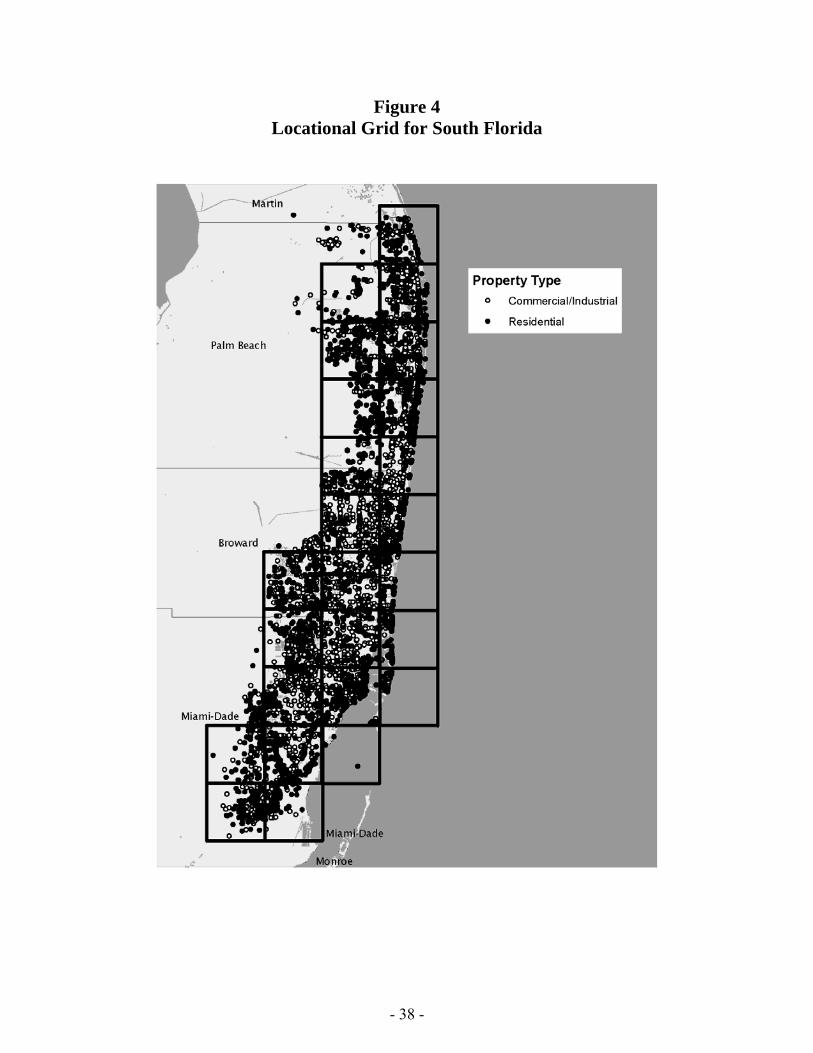
Figure 4 Locational Grid for South Florida

 

- 38 -

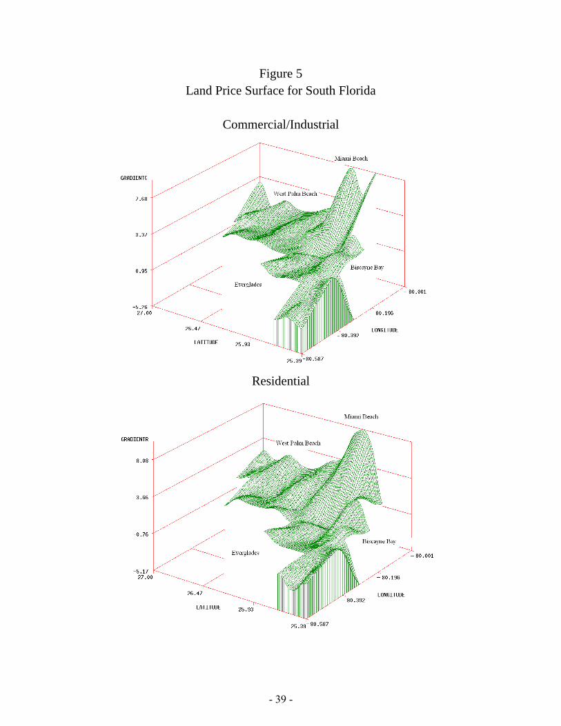
Figure 5 Land Price Surface for South Florida

Commercial/Industrial

 

Residential

 

- 39 -

1995 1997 1999 2001 2003 2005 2007 2009 0

50

100

150

200

250

Index, 2002:H2 = 100

Commercial/IndustrialResidential

Property Type Indexes

H1

1995 1997 1999 2001 2003 2005 2007 2009 0

50

100

150

200

250

Index, 2002:H2 = 100Composite of Commercial/Industrial and Residential Land Prices

H1

Figure 6National Land Price Indexes

Source. Authors’ analysis of data from the CoStar Group, Inc.

- 40 -

1996 2000 2004 2008 0

50

100

150

200

250

300

350

400

450

Index, 2002:H2 = 100

Washington, DCNew York City

1996 2000 2004 2008 0

50

100

150

200

250

300

350

400

450

Index, 2002:H2 = 100

South FloridaTampaOrlando

1996 2000 2004 2008 0

50

100

150

200

250

300

350

400

450

Index, 2002:H2 = 100

PhiladelphiaBostonBaltimore

1996 2000 2004 2008 0

50

100

150

200

250

300

350

400

450

Index, 2002:H2 = 100

Los AngelesSan Diego

1996 2000 2004 2008 0

50

100

150

200

250

300

350

400

450

Index, 2002:H2 = 100

San FranciscoSacramento

1996 2000 2004 2008 0

50

100

150

200

250

300

350

400

450

Index, 2002:H2 = 100

SeattlePortland

1996 2000 2004 2008 0

50

100

150

200

250

300

350

400

450

Index, 2002:H2 = 100

Las VegasTucsonPhoenix

1996 2000 2004 2008 0

50

100

150

200

250

300

350

400

450

Index, 2002:H2 = 100

AtlantaChicagoDetroit

1996 2000 2004 2008 0

50

100

150

200

250

300

350

400

450

Index, 2002:H2 = 100

HoustonDallasDenver

Figure 7Aggregate Land Price Indexes by MSA

Note. Shading begins immediately after 2009:H1.

- 41 -

1996 2000 2004 2008 0

50

100

150

200

250

300

350

400

450

Index, 2002:H2 = 100

Washington, DCNew York City

1996 2000 2004 2008 0

50

100

150

200

250

300

350

400

450

Index, 2002:H2 = 100

South FloridaTampaOrlando

1996 2000 2004 2008 0

50

100

150

200

250

300

350

400

450

Index, 2002:H2 = 100

PhiladelphiaBostonBaltimore

• •

1996 2000 2004 2008 0

50

100

150

200

250

300

350

400

450

Index, 2002:H2 = 100

1996 2000 2004 2008 0

50

100

150

200

250

300

350

400

450

Index, 2002:H2 = 100

Los AngelesSan Diego

1996 2000 2004 2008 0

50

100

150

200

250

300

350

400

450

Index, 2002:H2 = 100

San FranciscoSacramento

••

1996 2000 2004 2008 0

50

100

150

200

250

300

350

400

450

Index, 2002:H2 = 100

1996 2000 2004 2008 0

50

100

150

200

250

300

350

400

450

Index, 2002:H2 = 100

SeattlePortland

1996 2000 2004 2008 0

50

100

150

200

250

300

350

400

450

Index, 2002:H2 = 100

Las VegasTucsonPhoenix

1996 2000 2004 2008 0

50

100

150

200

250

300

350

400

450

Index, 2002:H2 = 100

AtlantaChicagoDetroit

1996 2000 2004 2008 0

50

100

150

200

250

300

350

400

450

Index, 2002:H2 = 100

HoustonDallasDenver

Figure 8Commercial/Industrial Land Price Indexes by MSA

Note. Shading begins immediately after 2009:H1. Segments between dots represent interpolation for missing half-yearly estimates.

- 42 -

1996 2000 2004 2008 0

50

100

150

200

250

300

350

400

450

Index, 2002:H2 = 100

Washington, DCNew York City

1996 2000 2004 2008 0

50

100

150

200

250

300

350

400

450

Index, 2002:H2 = 100

South FloridaTampaOrlando

•

•

1996 2000 2004 2008 0

50

100

150

200

250

300

350

400

450

Index, 2002:H2 = 100

1996 2000 2004 2008 0

50

100

150

200

250

300

350

400

450

Index, 2002:H2 = 100

PhiladelphiaBostonBaltimore

•

•

1996 2000 2004 2008 0

50

100

150

200

250

300

350

400

450

Index, 2002:H2 = 100

1996 2000 2004 2008 0

50

100

150

200

250

300

350

400

450

Index, 2002:H2 = 100

Los AngelesSan Diego

• • •

•

•

1996 2000 2004 2008 0

50

100

150

200

250

300

350

400

450

Index, 2002:H2 = 100

•

1996 2000 2004 2008 0

50

100

150

200

250

300

350

400

450

Index, 2002:H2 = 100

1996 2000 2004 2008 0

50

100

150

200

250

300

350

400

450

Index, 2002:H2 = 100

San FranciscoSacramento

• • ••

1996 2000 2004 2008 0

50

100

150

200

250

300

350

400

450

Index, 2002:H2 = 100

1996 2000 2004 2008 0

50

100

150

200

250

300

350

400

450

Index, 2002:H2 = 100

SeattlePortland

1996 2000 2004 2008 0

50

100

150

200

250

300

350

400

450

Index, 2002:H2 = 100

Las VegasTucsonPhoenix

1996 2000 2004 2008 0

50

100

150

200

250

300

350

400

450

Index, 2002:H2 = 100

AtlantaChicagoDetroit

• •

1996 2000 2004 2008 0

50

100

150

200

250

300

350

400

450

Index, 2002:H2 = 100

1996 2000 2004 2008 0

50

100

150

200

250

300

350

400

450

Index, 2002:H2 = 100

DallasDenver

•• •

•

1996 2000 2004 2008 0

50

100

150

200

250

300

350

400

450

Index, 2002:H2 = 100

Figure 9Residential Land Price Indexes by MSA

Note. Shading begins immediately after 2009:H1. Segments between dots represent interpolation for missing half-yearly estimates.Houston not shown due to small number of half-yearly estimates. - 43 -

- 44 -

Appendix

This appendix presents the results of a large set of likelihood ratio tests for the

equality of coefficients in our hedonic regression equation. For each hypothesis, the test

statistic is -2 ln(λR/λU), where λR is the value of the likelihood function after the equality

restrictions have been imposed and λU is the value of the unrestricted likelihood function.

This statistic is distributed χ2(ρ), where ρ equals the number of restrictions imposed by

the null hypothesis.

Each column in table A.1 reports the test results for a subset of independent

variables. The column labeled “Condition of property,” for example, includes the nine

dummy variables that fall under this heading, for which the coefficient estimates were

summarized in table 2. Similarly, the column labeled “Time effects” includes the full set

of half-yearly dummy variables. For any column in the table, the first row shows the

results for the most restrictive null hypothesis – that every variable in that column has a

single coefficient across all 23 MSAs and both property types. The second row tests a

less restrictive null hypothesis – that each variable has a single coefficient across all

MSAs for residential land and a separate coefficient across all MSAs for

commercial/industrial land. The next row tests the analogous null within MSAs – that

each variable has a single coefficient across residential and commercial/industrial land in

every MSA but that this coefficient differs across MSAs. The remaining rows test the

hypothesis that each variable has the same coefficient across the two property types for

MSAs taken one at a time.

Each entry in table A.1 presents the p-value for a particular hypothesis test. p-

values smaller than 0.05 indicate that the null hypothesis is rejected at the five-percent

- 45 -

level of significance, while p-values smaller than 0.001 indicate rejection at the one-

percent level. The p-values greater than 0.05 have been shaded to highlight the

hypotheses that cannot be rejected at the standard five-percent level.

The results in the first three lines of the table provide strong evidence in favor of

the highly disaggregated regression model that we estimate instead of a model that

aggregates the individual MSAs, the two broad property types, or both. As shown, all of

these aggregation hypotheses are rejected at the one-percent level of significance.1

The remaining rows of the table show that some of the coefficient restrictions

cannot be rejected for individual MSAs. For example, in 13 of the 23 MSAs we cannot

reject the hypothesis that distance from the CBD has the same price effect on residential

and commercial/industrial land. Similarly, in nine MSAs we cannot reject the hypothesis

that parcel size has the same price effect on both types of property. However, in every

MSA at least some of the equality restrictions are rejected at the one-percent level.

Accordingly, it is not appropriate to estimate an aggregated model for residential and

commercial/industrial land prices in any of the MSAs.

1 Note that we do not test the equality of the locational grids across MSAs. Given the differences in geographic features across MSAs, we would expect the price surfaces to differ as well.

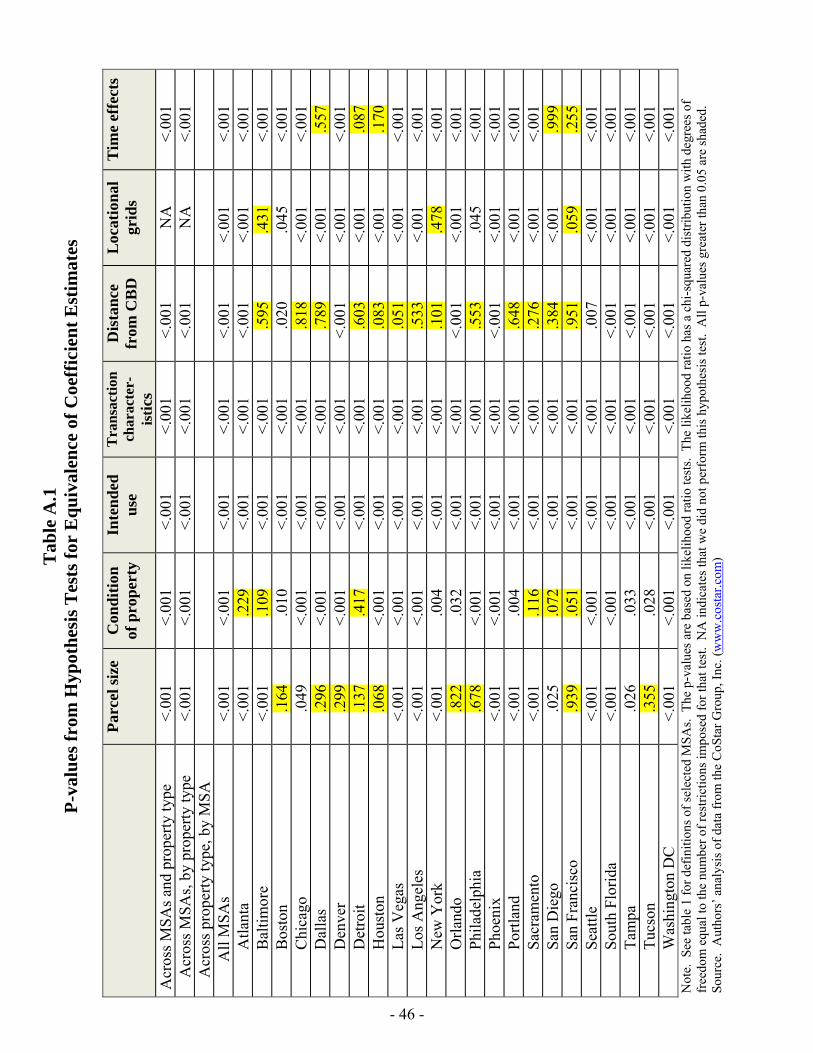
Tab

le A

.1

P-v

alu

es f

rom

Hyp

oth

esis

Tes

ts f

or E

qu

ival

ence

of

Coe

ffic

ien

t E

stim

ates

P

arce

l siz

e C

ond

itio

n

of p

rop

erty

In

ten

ded

u

se

Tra

nsa

ctio

n

char

acte

r-is

tics

Dis

tan

ce

from

CB

D

Loc

atio

nal

gr

ids

T

ime

effe

cts

Acr

oss M

SAs a

nd p

rope

rty ty

pe

<.00

1 <.

001

<.00

1 <.

001

<.00

1 N

A

<.00

1

Acr

oss M

SAs,

by p

rope

rty ty

pe

<.00

1 <.

001

<.00

1 <.

001

<.00

1 N

A

<.00

1

Acr

oss p

rope

rty ty

pe, b

y M

SA

A

ll M

SAs

<.00

1 <.

001

<.00

1 <.

001

<.00

1 <.

001

<.00

1

Atla

nta

<.00

1 .2

29

<.00

1 <.

001

<.00

1 <.

001

<.00

1

Bal

timor

e <.

001

.109

<.

001

<.00

1 .5

95

.431

<.

001

B

osto

n .1

64

.010

<.

001

<.00

1 .0

20

.045

<.

001

C

hica

go

.049

<.

001

<.00

1 <.

001

.818

<.

001

<.00

1

Dal

las

.296

<.

001

<.00

1 <.

001

.789

<.

001

.557

Den

ver

.299

<.

001

<.00

1 <.

001

<.00

1 <.

001

<.00

1

Det

roit

.137

.4

17

<.00

1 <.

001

.603

<.

001

.087

Hou

ston

.0

68

<.00

1 <.

001

<.00

1 .0

83

<.00

1 .1

70

L

as V

egas

<.

001

<.00

1 <.

001

<.00

1 .0

51

<.00

1 <.

001

L

os A

ngel

es

<.00

1 <.

001

<.00

1 <.

001

.533

<.

001

<.00

1

New

Yor

k <.

001

.004

<.

001

<.00

1 .1

01

.478

<.

001

O

rland

o .8

22

.032

<.

001

<.00

1 <.

001

<.00

1 <.

001

P

hila

delp

hia

.678

<.

001

<.00

1 <.

001

.553

.0

45

<.00

1

Pho

enix

<.

001

<.00

1 <.

001

<.00

1 <.

001

<.00

1 <.

001

P

ortla

nd

<.00

1 .0

04

<.00

1 <.

001

.648

<.

001

<.00

1

Sac

ram

ento

<.

001

.116

<.

001

<.00

1 .2

76

<.00

1 <.

001

S

an D

iego

.0

25

.072

<.

001

<.00

1 .3

84

<.00

1 .9

99

S

an F

ranc

isco

.9

39

.051

<.

001

<.00

1 .9

51

.059

.2

55

S

eattl

e <.

001

<.00

1 <.

001

<.00

1 .0

07

<.00

1 <.

001

S

outh

Flo

rida

<.00

1 <.

001

<.00

1 <.

001

<.00

1 <.

001

<.00

1

Tam

pa

.026

.0

33

<.00

1 <.

001

<.00

1 <.

001

<.00

1

Tuc

son

.355

.0

28

<.00

1 <.

001

<.00

1 <.

001

<.00

1

Was

hing

ton

DC

<.

001

<.00

1 <.

001

<.00

1 <.

001

<.00

1 <.

001

Not

e. S

ee ta

ble

1 fo

r def

initi

ons o

f sel

ecte

d M

SAs.

The

p-v

alue

s are

bas

ed o

n lik

elih

ood

ratio

test

s. T

he li

kelih

ood

ratio

has

a c

hi-s

quar

ed d

istri

butio

n w

ith d

egre

es o

f fr

eedo

m e

qual

to th

e nu

mbe

r of r

estri

ctio

ns im

pose

d fo

r tha

t tes

t. N

A in

dica

tes t

hat w

e di

d no

t per

form

this

hyp

othe

sis t

est.

All

p-va

lues

gre

ater

than

0.0

5 ar

e sh

aded

. So

urce

. A

utho

rs’ a

naly

sis o

f dat

a fr

om th

e C

oSta

r Gro

up, I

nc. (

ww

w.c

osta

r.com

)

- 46 -