finalreport - university transportation research center measures to characterize ... negotiation...

Final

January 2016

University Transportation Research Center - Region 2

ReportPerforming Organization: The College of New Jersey

Performance Measures To Characterize Directional Corridor Travel Time Delay Based On Probe Vehicle Data

Sponsor:University Transportation Research Center - Region 2

University Transportation Research Center - Region 2

The Region 2 University Transportation Research Center (UTRC) is one of ten original University Transportation Centers established in 1987 by the U.S. Congress. These Centers were established with the recognition that transportation plays a key role in the nation's economy and the quality of life of its citizens. University faculty members provide a critical link in resolving our national and regional transportation problems while training the professionals who address our transpor-tation systems and their customers on a daily basis.

The UTRC was established in order to support research, education and the transfer of technology in the �ield of transportation. The theme of the Center is "Planning and Managing Regional Transportation Systems in a Changing World." Presently, under the direction of Dr. Camille Kamga, the UTRC represents USDOT Region II, including New York, New Jersey, Puerto Rico and the U.S. Virgin Islands. Functioning as a consortium of twelve major Universities throughout the region, UTRC is located at the CUNY Institute for Transportation Systems at The City College of New York, the lead institution of the consortium. The Center, through its consortium, an Agency-Industry Council and its Director and Staff, supports research, education, and technology transfer under its theme. UTRC’s three main goals are:

Research

The research program objectives are (1) to develop a theme based transportation research program that is responsive to the needs of regional transportation organizations and stakehold-ers, and (2) to conduct that program in cooperation with the partners. The program includes both studies that are identi�ied with research partners of projects targeted to the theme, and targeted, short-term projects. The program develops competitive proposals, which are evaluated to insure the mostresponsive UTRC team conducts the work. The research program is responsive to the UTRC theme: “Planning and Managing Regional Transportation Systems in a Changing World.” The complex transportation system of transit and infrastructure, and the rapidly changing environ-ment impacts the nation’s largest city and metropolitan area. The New York/New Jersey Metropolitan has over 19 million people, 600,000 businesses and 9 million workers. The Region’s intermodal and multimodal systems must serve all customers and stakeholders within the region and globally.Under the current grant, the new research projects and the ongoing research projects concentrate the program efforts on the categories of Transportation Systems Performance and Information Infrastructure to provide needed services to the New Jersey Department of Transpor-tation, New York City Department of Transportation, New York Metropolitan Transportation Council , New York State Department of Transportation, and the New York State Energy and Research Development Authorityand others, all while enhancing the center’s theme.

Education and Workforce Development

The modern professional must combine the technical skills of engineering and planning with knowledge of economics, environmental science, management, �inance, and law as well as negotiation skills, psychology and sociology. And, she/he must be computer literate, wired to the web, and knowledgeable about advances in information technology. UTRC’s education and training efforts provide a multidisciplinary program of course work and experiential learning to train students and provide advanced training or retraining of practitioners to plan and manage regional transportation systems. UTRC must meet the need to educate the undergraduate and graduate student with a foundation of transportation fundamentals that allows for solving complex problems in a world much more dynamic than even a decade ago. Simultaneously, the demand for continuing education is growing – either because of professional license requirements or because the workplace demands it – and provides the opportunity to combine State of Practice education with tailored ways of delivering content.

Technology Transfer

UTRC’s Technology Transfer Program goes beyond what might be considered “traditional” technology transfer activities. Its main objectives are (1) to increase the awareness and level of information concerning transportation issues facing Region 2; (2) to improve the knowledge base and approach to problem solving of the region’s transportation workforce, from those operating the systems to those at the most senior level of managing the system; and by doing so, to improve the overall professional capability of the transportation workforce; (3) to stimulate discussion and debate concerning the integration of new technologies into our culture, our work and our transportation systems; (4) to provide the more traditional but extremely important job of disseminating research and project reports, studies, analysis and use of tools to the education, research and practicing community both nationally and internationally; and (5) to provide unbiased information and testimony to decision-makers concerning regional transportation issues consistent with the UTRC theme.

Project No(s): UTRC/RF Grant No: 49997-18-25

Project Date: October 2015

Project Title: Performance Measures To Characterize Directional Corridor Travel Time Delay Based On Probe Vehicle Data

Project’s Website: http://www.utrc2.org/research/projects/highway-corridor-length Principal Investigator(s):

Dr. Thomas M. Brennan Jr.Assistant ProfessorCivil EngineeringThe College of New JerseyEwing, NJ 08628 Tel: (609) 771-2475Fax: (609) 637-2538Email: [email protected]

Performing Organization: The College of New Jersey

Sponsor(s):)University Transportation Research Center (UTRC)

To request a hard copy of our �inal reports, please send us an email at [email protected]

Mailing Address:

University Transportation Reserch CenterThe City College of New YorkMarshak Hall, Suite 910160 Convent AvenueNew York, NY 10031Tel: 212-650-8051Fax: 212-650-8374Web: www.utrc2.org

Board of Directors

The UTRC Board of Directors consists of one or two members from each Consortium school (each school receives two votes regardless of the number of representatives on the board). The Center Director is an ex-of icio member of the Board and The Center management team serves as staff to the Board.

City University of New York Dr. Hongmian Gong - Geography/Hunter College Dr. Neville A. Parker - Civil Engineering/CCNY

Clarkson University Dr. Kerop D. Janoyan - Civil Engineering

Columbia University Dr. Raimondo Betti - Civil Engineering Dr. Elliott Sclar - Urban and Regional Planning

Cornell University Dr. Huaizhu (Oliver) Gao - Civil Engineering

Hofstra University Dr. Jean-Paul Rodrigue - Global Studies and Geography

Manhattan College Dr. Anirban De - Civil & Environmental Engineering Dr. Matthew Volovski - Civil & Environmental Engineering

New Jersey Institute of Technology Dr. Steven I-Jy Chien - Civil Engineering Dr. Joyoung Lee - Civil & Environmental Engineering

New York University Dr. Mitchell L. Moss - Urban Policy and Planning Dr. Rae Zimmerman - Planning and Public Administration

Polytechnic Institute of NYU Dr. Kaan Ozbay - Civil Engineering Dr. John C. Falcocchio - Civil Engineering Dr. Elena Prassas - Civil Engineering

Rensselaer Polytechnic Institute Dr. José Holguín-Veras - Civil Engineering Dr. William "Al" Wallace - Systems Engineering

Rochester Institute of Technology Dr. James Winebrake - Science, Technology and Society/Public Policy Dr. J. Scott Hawker - Software Engineering

Rowan University Dr. Yusuf Mehta - Civil Engineering Dr. Beena Sukumaran - Civil Engineering

State University of New York Michael M. Fancher - Nanoscience Dr. Catherine T. Lawson - City & Regional Planning Dr. Adel W. Sadek - Transportation Systems Engineering Dr. Shmuel Yahalom - Economics

Stevens Institute of Technology Dr. Sophia Hassiotis - Civil Engineering Dr. Thomas H. Wakeman III - Civil Engineering

Syracuse University Dr. Riyad S. Aboutaha - Civil Engineering Dr. O. Sam Salem - Construction Engineering and Management

The College of New Jersey Dr. Thomas M. Brennan Jr - Civil Engineering

University of Puerto Rico - Mayagüez Dr. Ismael Pagán-Trinidad - Civil Engineering Dr. Didier M. Valdés-Díaz - Civil Engineering

UTRC Consortium Universities

The following universities/colleges are members of the UTRC consor-tium.

City University of New York (CUNY)Clarkson University (Clarkson)Columbia University (Columbia)Cornell University (Cornell)Hofstra University (Hofstra)Manhattan College (MC)New Jersey Institute of Technology (NJIT)New York Institute of Technology (NYIT)New York University (NYU)Rensselaer Polytechnic Institute (RPI)Rochester Institute of Technology (RIT)Rowan University (Rowan)State University of New York (SUNY)Stevens Institute of Technology (Stevens)Syracuse University (SU)The College of New Jersey (TCNJ)University of Puerto Rico - Mayagüez (UPRM)

UTRC Key Staff

Dr. Camille Kamga: Director, Assistant Professor of Civil Engineering

Dr. Robert E. Paaswell: Director Emeritus of UTRC and Distinguished Professor of Civil Engineering, The City College of New York

Herbert Levinson: UTRC Icon Mentor, Transportation Consultant and Professor Emeritus of Transportation

Dr. Ellen Thorson: Senior Research Fellow, University Transportation Research Center

Penny Eickemeyer: Associate Director for Research, UTRC

Dr. Alison Conway: Associate Director for Education

Nadia Aslam: Assistant Director for Technology Transfer

Nathalie Martinez: Research Associate/Budget Analyst

Tierra Fisher: Of ice Assistant

Bahman Moghimi: Research Assistant; Ph.D. Student, Transportation Program

Wei Hao: Research Fellow

Andriy Blagay: Graphic Intern

Membership as of January 2016

TECHNICAL REPORT STANDARD TITLE PAGE

1. Report No. 2.Government Accession No. 3. Recipient’s Catalog No.

UTRC: 49997-18-25

4. Title and Subtitle 5. Report Date

PERFORMANCE MEASURES TO CHARACTERIZE DIRECTIONAL CORRIDOR TRAVEL TIME DELAY BASED ON PROBE VEHICLE DATA 6. Performing Organization Code

7. Author(s) 8. Performing Organization Report No.

Thomas M. Brennan Jr. P.E, Ph.D.

9. Performing Organization Name and Address 10. Work Unit No.

The College of New Jersey 2000 Pennington Road Ewing, NJ 08628

11. Contract or Grant No.

12. Sponsoring Agency Name and Address 13. Type of Report and Period Covered University Transportation Research Center Marshak Hall - Science Building, Suite 910 The City College of New York 138th Street & Convent Avenue ,New York, NY 10031

14. Sponsoring Agency Code

15. Supplementary Notes

16. Abstract

17. Key Words 18. Distribution Statement

Probe Vehicles, Travel Time Analysis, Data Collection

19. Security Classif (of this report) 20. Security Classif. (of this page) 21. No of Pages 22. Price

Unclassified Unclassified

34

Form DOT F 1700.7 (8-69)

49997-18-25

final, Jan. 1, 2014 -June 30, 2015

brennant

Typewritten Text

January 2016

brennant

Typewritten Text

brennant

Typewritten Text

brennant

Typewritten Text

brennant

Typewritten Text

brennant

Typewritten Text

brennant

Typewritten Text

Anonymous probe vehicle data are currently being collected on roadways throughout the United States. These data are being incorporated into local and statewide mobility reports to measure the performance of freeways and arterial systems. Predefined spatially located segments, known as Traffic Message Channels (TMCs), are spatially and temporally joined with probe vehicle speed data. Through the analysis these data, transportation agencies have been developing agency wide travel time performance measures. One widely accepted performance measure is travel time reliability, which is calculated along a series of TMCs. Travel time reliability is usually measured as a percentile of base travel time or speed. When reliable travel times are not achieved because of incidents and recurring congestion, it is desirable to understand the time and location of these occurrences to proactively manage the corridor. This research emphasizes a visually intuitive methodology that aggregates a series of TMC segments based on a cursory review of congestion hot spots within a corridor. Instead of a fixed congestion speed threshold, each TMC link is assigned a congestion threshold based on the 70th percentile of the 15-minute average speeds between 2AM and 6AM. An analysis of approximately 90-million speed records collected in 2013 along I-80 in northern New Jersey was performed for this project. Travel Time Inflation, the time exceeding the expected travel time at 70% of measured free flow speed, was used to evaluate each of the 166 directional TMC segments along 70 miles of I-80. This performance measure accounts for speed variability caused by roadway geometry, heavy traffic flows, and other Highway Capacity Manual speed-reducing friction-factors associated with each TMC. A t-stat analysis based on unequal means was conducted to compare each of the TMC segments to determine statistical similarities of adjacent TMCs. An example analysis of 5 Million records in 2013 during the AM Peak eastbound direction of I-80 in northern New Jersey was performed for this research. The results determined that of the 83 segments in the eastbound direction there were 25 statistically similar groups.

Brennan UTRC 49997-18-25

i

Disclaimer

The contents of this report reflect the views of the authors, who are responsible for the facts and

the accuracy of the information presented herein. The contents do not necessarily reflect the

official views or policies of the UTRC or the Federal Highway Administration. This report does

not constitute a standard, specification or regulation. This document is disseminated under the

sponsorship of the Department of Transportation, University Transportation Centers Program, in

the interest of information exchange. The U.S. Government assumes no liability for the contents

or use thereof


ii

ACKNOWLEDGMENTS

The authors would like to thank the Coordenação de Aperfeiçoamento de Pessoal de Nível

Superior (CAPES) Foundation - Ministry of Education of Brazil for providing funding for our

undergraduate researchers. The contents of this report reflect the views of the authors, who are

responsible for the facts and the accuracy of the data presented herein, and do not necessarily reflect the

official views or policies of the sponsoring organizations. These contents do not constitute a standard,

specification, or regulation. This research is being funded by the Region 2- University Transportation

Research Center (UTRC). The speed data and segment information used in this report was obtained

from INRIX Inc.


iii

FIGURES

Figure 1. I-80 Corridor in northern New Jersey. .......................................................................................... 5

Figure 2. Aggregated directional congestion hours. .................................................................................... 8

Figure 3. I-80 Congestion Hours below a variable congestion threshold speed in 2013. ............................ 9

Figure 4. Total hours of Travel Time Inflation based on Variable Threshold Congestion Speed. ............ 11

Figure 5. One-week example of 24-hour plots of Corridor Travel Time Inflation between westbound

mile markers 52.5 – 39.6. ........................................................................................................... 13

Figure 6. Plan layout of 24-hour plots of Corridor Travel Time Inflation for westbound mile markers

52.5 – 39.6. ................................................................................................................................. 14

Figure 7. Isometric layout of 24-hour plots of Corridor Travel Time Inflation for westbound mile

markers 52.5 – 39.6. ................................................................................................................... 15

Figure 8. One year of 24-hour plots of Corridor Travel Time Inflation for westbound mile markers 52.5

– 39.6. ......................................................................................................................................... 17


markers 52.5 – 39.6. ................................................................................................................... 18

Figure 10. The contributing values of each of the 14 segments on the CTI values for the I-80 westbound

corridor from MM 52.5 – 39.6 during the February 8, 2014 winter storm. ................................ 18

Figure 11. Side by side layout of Corridor Travel Time Inflation plot for eastbound and for westbound

I-80 traffic between mile markers 52.5 – 39.6. ........................................................................... 20

Figure 12. Total hours of Travel Time Inflation based on Variable Threshold Congestion Speed. .......... 21

Figure 13. Relative differences between the mean values of the average percent increase in travel time

per month. ................................................................................................................................... 23

Figure 14. AM Peak eastbound differences between the mean values of the average percent increase in

travel time I-80 ........................................................................................................................... 24

TABLES

Table 1. Example of TMC network spatial attributes .................................................................................. 6

Table 2. Example of 15-minute binned probe data with TMC speeds. ......................................................... 6

Table 3. T-Test grouping of 83 eastbound AM Peak travel time highway segments along I-80, 2013 ...... 25

Table 4. ANOVA analysis for six segments between MM 39.9 – 43.2 ..................................................... 27


1

ABSTRACT

Anonymous probe vehicle data are currently being collected on roadways throughout the United

States. These data are being incorporated into local and statewide mobility reports to measure the

performance of freeways and arterial systems. Predefined spatially located segments, known as Traffic

Message Channels (TMCs), are spatially and temporally joined with probe vehicle speed data. Through

the analysis of these data, transportation agencies have been developing agency wide travel time

performance measures. One widely accepted performance measure is travel time reliability, which is

calculated along a series of TMCs. Travel time reliability is usually measured as a percentile of base

travel time or speed. When reliable travel times are not achieved because of incidents and recurring

congestion, it is desirable to understand the time and location of these occurrences to proactively

manage the corridor.

This research emphasizes a visually intuitive methodology that aggregates a series of TMC

segments based on a cursory review of congestion hot spots within a corridor. Instead of a fixed

congestion speed threshold, each TMC link is assigned a congestion threshold based on the 70th

percentile of the 15-minute average speeds between 2AM and 6AM. An analysis of approximately 90-

million speed records collected in 2013 along I-80 in northern New Jersey was performed for this

project. Travel Time Inflation, the time exceeding the expected travel time at 70% of measured free

flow speed, was used to evaluate each of the 166 directional TMC segments along 70 miles of I-80. This

performance measure accounts for speed variability caused by roadway geometry, heavy traffic flows,

and other Highway Capacity Manual speed-reducing friction-factors associated with each TMC.

A t-stat analysis based on unequal means was conducted to compare each of the TMC segments

to determine statistical similarities of adjacent TMCs. An example analysis of 5 Million records in 2013

during the AM Peak eastbound direction of I-80 in northern New Jersey was performed for this

research. The results determined that of the 83 segments in the eastbound direction there were 25

statistically similar groups.


2

EXECUTIVE SUMMARY

A complete paper can be found in the Transportation Research Record (1) and the compendium

of papers for the ITS World Congress in Bordeaux (2). Based on the research, it is concluded that the

uses of a variable free flow travel time evaluated on a fixed length highway segment, or Traffic Message

Change (TMC), using anonymous prove vehicle data provides a means to account for variably in driver

free flow speed caused by exterior factors as indicated by the Highway Capacity Manual (e.g. lane

widths, shoulder width, etc…). For this research, the proposed 70% of the base free flow speed

accounts for some of the free flow speed reduction friction factors identified by the highway capacity

manual (HCM) along a TMC link. This percentage can be adjusted, but the 70% values has been used

in previous research and is a good indication when congestion condition occur. Although a

comprehensive view of the actual infrastructure was not conducted, it is a reasonable expectation that

the geometric layout and other contributing factors associated with a highway segment will impact a

TMC’s base free flow speed, and ultimately the point when a TMC is considered to be congested. This

new performance measure is graphically presented over a long period of time with intuitive two-

dimensional and three-dimensional graphical representation of the travel times obtained from

anonymous probe vehicle data. Additional findings indicated that fixed highway segments could be

grouped based on similar travel times using a T-Test of adjacent segments. The results showed that out

of 83 fixed highway segments, 25 groups or corridors, could be identified.


3

INTRODUCTION AND BACKGROUND

The development of travel time reliability performance measures using probe vehicle data is

being addressed across the country to satisfy the performance-based portions of the Moving Ahead for

Progress in the 21st Century Act (MAP-21). MAP-21 (3) is a 2-year $105 billion surface transportation

bill initiative that has provisions for better data collection of highway performance monitoring,

continuous travel monitoring, and analysis. Probe vehicle speeds and location data provide a means to

monitor and proactively manage highway systems. Each system experiences a variable number of

conditions including weather, crash incidents, geometry layout, and construction. These data are also

being used to identify areas of the nation’s roadway infrastructure in need of improvement. Currently,

the United States (US) holds a grade of ‘D’ by the American Society of Civil Engineering (ASCE) for

roads (4), meaning that a large number of US roadways that remain congested. With a better

understanding of the location, frequency, type of roadway congestion occurrences, and travel time

reliability over a defined corridor a better capital improvement management plans can be developed.

There have been a number of reports developed in recent years using anonymous probe vehicle

data. The Texas A&M Transportation Institute applied this type of data for their analysis in their

national mobility reports that focused on city and urban centers for their Urban Mobility Reports (5, 6).

Indiana has developed performance measures to rank interstate freeways on a statewide level, including

commuter corridors (7, 8, 9) using different performance methods. Other agencies have also begun to

use this data in their annual reports (10, 11, 12, 13). As probe vehicle data and other types of crowd

data sources become more reliable, it is expected that performance measures developed from this data

will also become more relevant. Before 2010, probe vehicle data was presented in 5-minute increments

and it did not cover all major interstates and highways. However, since 2010 the fidelity of probe

vehicle data has improved greatly and now includes both public and private crowd sources (8).

Congestion is defined in a number of research publications that include a binary measure of

congestion hours, congestion index, and weighted congestion hours (14). These performance measures


4

work well, but they do not account of speed variation across the system due to changes in posted speed

limits, geometric layout and roadway conditions. They instead rely on a fixed congestion threshold.

Other indices that account for travel time or travel time deficiency (9) provide an additional means to

measure travel time reliability, but remain associated with a fixed congestion speed threshold. The

research presented builds upon previously defined congestion performance measures (14, 15) which are

based on fixed speed threshold by proposing highway congestion performance measures that account

for speed variability between Traffic Message Channels (TMCs). The research concludes by presenting

an improved visualization for highway segment, and corridor performance which is currently in press

with the Transportation Research Record (1). In addition, this research proposes a quantitative grouping

of statically similar highway segments into defined travel corridors to better evaluate travel time

reliability under similar congestion conditions.

DATA

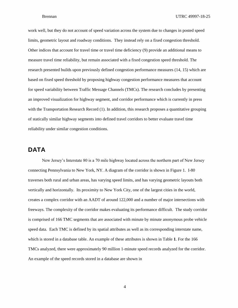
New Jersey’s Interstate 80 is a 70 mile highway located across the northern part of New Jersey

connecting Pennsylvania to New York, NY. A diagram of the corridor is shown in Figure 1. I-80

traverses both rural and urban areas, has varying speed limits, and has varying geometric layouts both

vertically and horizontally. Its proximity to New York City, one of the largest cities in the world,

creates a complex corridor with an AADT of around 122,000 and a number of major intersections with

freeways. The complexity of the corridor makes evaluating its performance difficult. The study corridor

is comprised of 166 TMC segments that are associated with minute by minute anonymous probe vehicle

speed data. Each TMC is defined by its spatial attributes as well as its corresponding interstate name,

which is stored in a database table. An example of these attributes is shown in Table 1. For the 166

TMCs analyzed, there were approximately 90 million 1-minute speed records analyzed for the corridor.

An example of the speed records stored in a database are shown in


5

Table 2. For this research only data points with a confidence score of 30 where used. This

score indicates that a speed measure was obtained directly from probe vehicles, as opposed to a score of

10 or 20, which would indicate the speed value was calculated based in part on historic data. Each

speed associated with a TMC was then aggregated into 15-minute space mean speed (SMS) bins, 96

total, over a 24 hour period for each day in 2013 and subsequently stored in a new database table. The

15-minute speeds associated with each TMC for each day of the year are subsequently used to develop

the traffic performance measure and visualization methods proposed in this report. The use of SMS

instead of average speed provides a more conservative estimate that accounts for the variability in

vehicle speed as it traverses a TMC.

To assess a series of TMCs as a defined corridor with similar speed patterns, the 15-minute

speeds associated with each TMC for each day of the year are subsequently used to develop a method to

group subsections of highway segments that experience similar congestion conditions (2). The use of

SMS accounts for the variability in vehicle speed as it traverses a TMC, while the aggregation method

will account for similar congestion conditions on adjacent segments.

Figure 1. I-80 Corridor in northern New Jersey.

Table 1. Example of Traffic Message Channel (TMC) network spatial attributes


6

TMC Road/

Direction

Length

(Miles)

Lat.

Start

Long.

Start

Lat.

End

Long.

End

103+05337 I-080 W 0.01535 39.0271 -74.4507 39.0325 -74.4674

103P05336 I-080 W 0.01338 39.0229 -74.4439 39.0271 -74.4507

103-05336 I-080 E 0.01338 39.0285 -74.4546 39.0321 -74.4546

103N0533 I-080 E 0.00415 39.0271 -74.4507 39.0285 -74.4546

Table 2. Example of 15-minute binned probe data with TMC speeds.

TMC Date Time Stamp SMS (MPH) Confidence Score

103+05337 2011-01-01 01:00:00 65 30

103+05337 2011-01-01 01:15:00 64 30

103P05336 2011-01-01 01:00:00 45 30

103P05336 2011-01-01 01:15:00 42 30

CONGESTION

Previous research has considered any TMC i to be congested during a period of time j when the

calculated SMS vij falls below a pre-defined speed threshold ve,, typically 45 mph for highways (7, 8,

15). Using a fixed speed threshold does not account for variations in the road geometry, the number of

ramps, changes in posted speed, or other highway capacity manual (HCM) speed-reducing friction

factors that can contribute to reduction in speed. Therefore, presented in this research is a variable

speed threshold used to compare against each calculated SMS (vij) over a 15-minute period. The

variable speed threshold is calculated using the following:

ij

ij

ia vn

v1

70.0 1

where via is the variable speed threshold, ijn is the total count of the 15-minute SMS bins between 0200

and 0600 hours for a full year. The SMS were calculated in the early morning hours when lower

volumes are present and vehicles are expected to be traveling in free flow conditions. A similar

approach, using a dynamic free flows speed based on the maximum average over a time period, was

used to evaluate congested conditions in a report by the European Joint Research Commission (16). The

variable via is based on 70 percent of the average SMS for the defined time period. The 70 percent can


7

be adjusted based on an agency’s need, but was chosen because previous studies used 45 MPH as the

fixed speed threshold, which is approximately 70% of 65 MPH (7,8). Other reports have suggested

threshold speeds around 35 mph in large urban areas and 55 mph in small urban areas (). A binary

indicator (15) was used to calculate the number of times an observed SMS fell below the variable

threshold value for a TMC as shown in the following:

iaij

iaij

ij vv

vv

,0

,1 2

where via is the variable congestion threshold speed for any TMC segment i during any 15-minute

period j andij is a binary indicator that equates to ‘1’ when the SMS falls below via .

Congestion Hours

Aggregating the frequency when a TMC segment falls below the binary congestion threshold

(via) provides a simplistic calculation to quickly identify areas where congestion may be of concern.

This aggregation has been defined in previous research (7, 8, 15) and is redefined in the following

equation:

Gi Tj

TGVCH ij, 25.0 3

where, VCH is the number of congestion hours based on a variable threshold speed, G represents the

group of TMC segments and T represents time periods being considered. The 0.25 constant aggregates

the 15-minute congestion periods into hours.

The fixed speed threshold (45mph) is compared to the variable speed threshold in Figure 2.

Using the variable speed provides a less conservative, but more accurate indication of congestion

because it accounts for speed variation between different TMCs. As shown in the figure, the use of the

variable speed threshold shows less congestion for the aggregated monthly congestion hours along I-80,

thus limiting the number of potential false congestion hour indications. The aggregation of each TMC’s

congestion is shown in Figure 3, which is adapted from previous research used to illustrate congestion

hours along a corridor (7, 8). Each TMC is represented by its mile marker (MM) designations, which


8

provides the relative length of each TMC segment along the corridor. The major change from previous

research is that for this graph the congestion speed threshold values vary for each TCM along the

corridor. Most of the congestion in Figure 3 appears to be recurring with the exception of the

westbound direction when higher values were observed in May, June, and July. The drawback with this

type of graph is that it does not show the intensity of the congestion, the time of day when congestion is

occurring and it does not account for the TMC length. The TMC length is important when comparing

longer and shorter segments that may have the same number of congestion hours. A longer segment will

inherently impact a greater number of drivers under equal volumes and lane numbers.

Figure 2. Aggregated directional congestion hours.

0

1000

2000

3000

4000

5000

6000

JAN FEB MAR APR MAY JUN JUL AUG SEP OCT NOV DEC

2013

I-80 FIXED THRESHOLD CONGESTION HOURS

I-80 VARIABLE THRESHOLD CONGESTION HOURS

CO

NG

ESTI

ON

HO

UR

S

Using Fixed 45 MPH Congestion Threshold

Using Variable Congestion Threshold


9

a) Eastbound

b) Westbound

Figure 3. I-80 Congestion Hours below a variable congestion threshold speed in 2013.

Travel Time Inflation

The Travel Time Inflation (TI) performance measure was developed to take into account both

the distance and speeds for each TMC. Similar to the variable speed congestion hours, each TMC is

assigned a base travel time (BTT) that accounts for the TMC’s length and observed 70th percentile free

flow speed. The base travel time for each TMC is a function of the variable threshold speed and is

defined in the following:

ia

ii

v

xBTT 4

Where BTTi is the base travel time in hours for TMC i and xi is the distance in miles for the TMC. Any

increase in travel time will occur when the binary indicator defined in Eq.2 (ij ) is equal to 1. The

travel time for any TMC segment is defined as the following:

0

300

600

900

1200

1500

0.0

5.0

10.

0

15.

0

20.

0

25.

0

30.

0

35.

0

40.

0

45.

0

50.

0

55.

0

60.

0

65.

0

DecNovOctSepAugJulJunMayAprMarFebJan

Mile Markers (East Bound )

Co

nge

stio

n H

ou

rs Recurring CongestionRecurring Congestion

0

300

600

900

1200

1500

0.0

5.0

10.

0

15.

0

20.

0

25.

0

30.

0

35.

0

40.

0

45.

0

50.

0

55.

0

60.

0

65.

0


Mile Markers (West Bound )

Co

nge

stio

n H

ou

rs

Higher Congestion Hours in May, June, July

Recurring Congestion


10

iaij

iaij

ij

i

ij

vv

vvv

x

TT

,0

, 5

where TTij is travel time in hours of TMC i at time period j. The travel time is only calculated when the

observed speed vij is less than the variable threshold speed via. When vij is greater than the variable

threshold speed via, the level of congestion is considered to be above the threshold and therefore not

counted resulting in TTij = 0. It is the summation of the difference between the actual travel time and the

base travel time that is used to define TI, which is shown in the following:

n

j

iiji BTTTTTI1

)( 6

where TIi is the total Travel Time Inflation for TMC segment i for all 15-minute bin time periods j

within a time frame defined by the analyst. The TI performance measure takes into account the time it

takes to traverse a segment. By aggregating the TI values over time, a representation of the relative

congestion intensity can be evaluated. Using travel time inherently weights the distance when

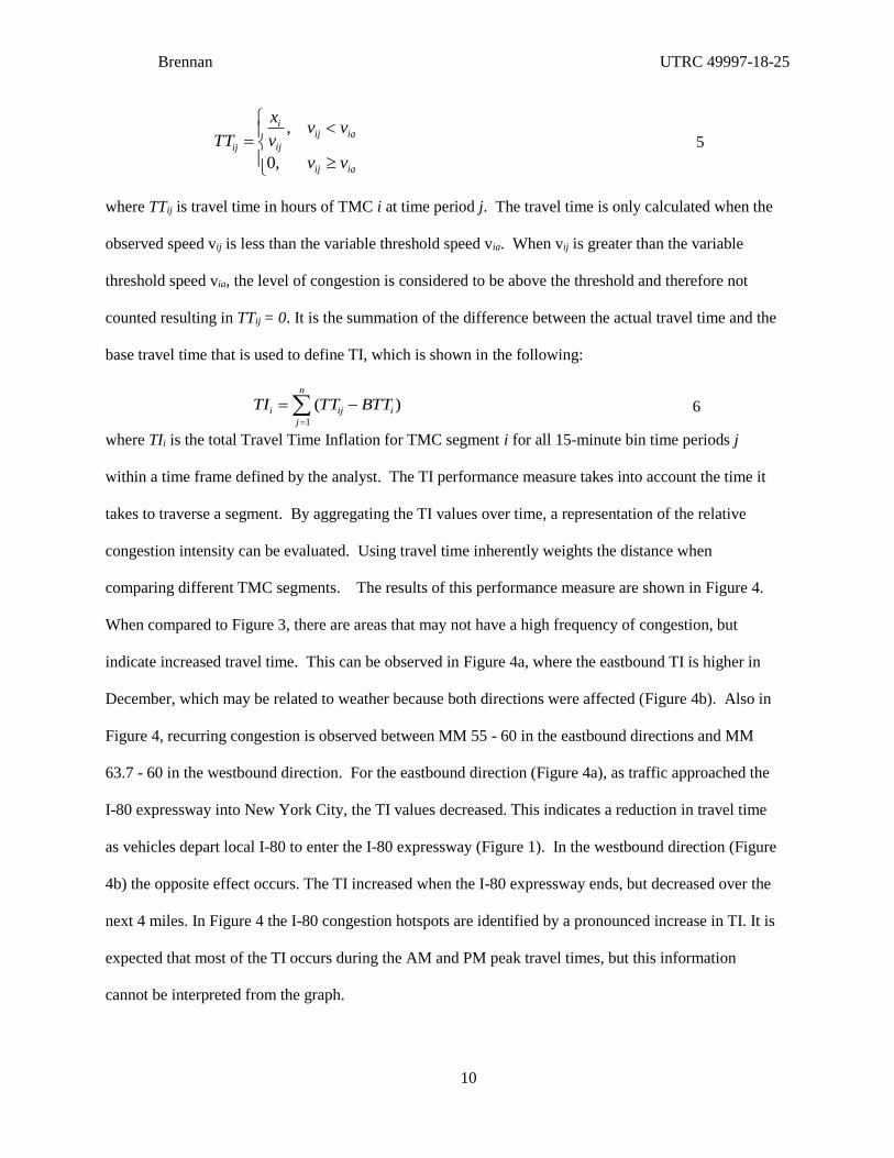
comparing different TMC segments. The results of this performance measure are shown in Figure 4.

When compared to Figure 3, there are areas that may not have a high frequency of congestion, but

indicate increased travel time. This can be observed in Figure 4a, where the eastbound TI is higher in

December, which may be related to weather because both directions were affected (Figure 4b). Also in

Figure 4, recurring congestion is observed between MM 55 - 60 in the eastbound directions and MM

63.7 - 60 in the westbound direction. For the eastbound direction (Figure 4a), as traffic approached the

I-80 expressway into New York City, the TI values decreased. This indicates a reduction in travel time

as vehicles depart local I-80 to enter the I-80 expressway (Figure 1). In the westbound direction (Figure

4b) the opposite effect occurs. The TI increased when the I-80 expressway ends, but decreased over the

next 4 miles. In Figure 4 the I-80 congestion hotspots are identified by a pronounced increase in TI. It is

expected that most of the TI occurs during the AM and PM peak travel times, but this information

cannot be interpreted from the graph.


11

a) Eastbound

b) Westbound

Figure 4. Total hours of Travel Time Inflation based on Variable Threshold Congestion Speed.

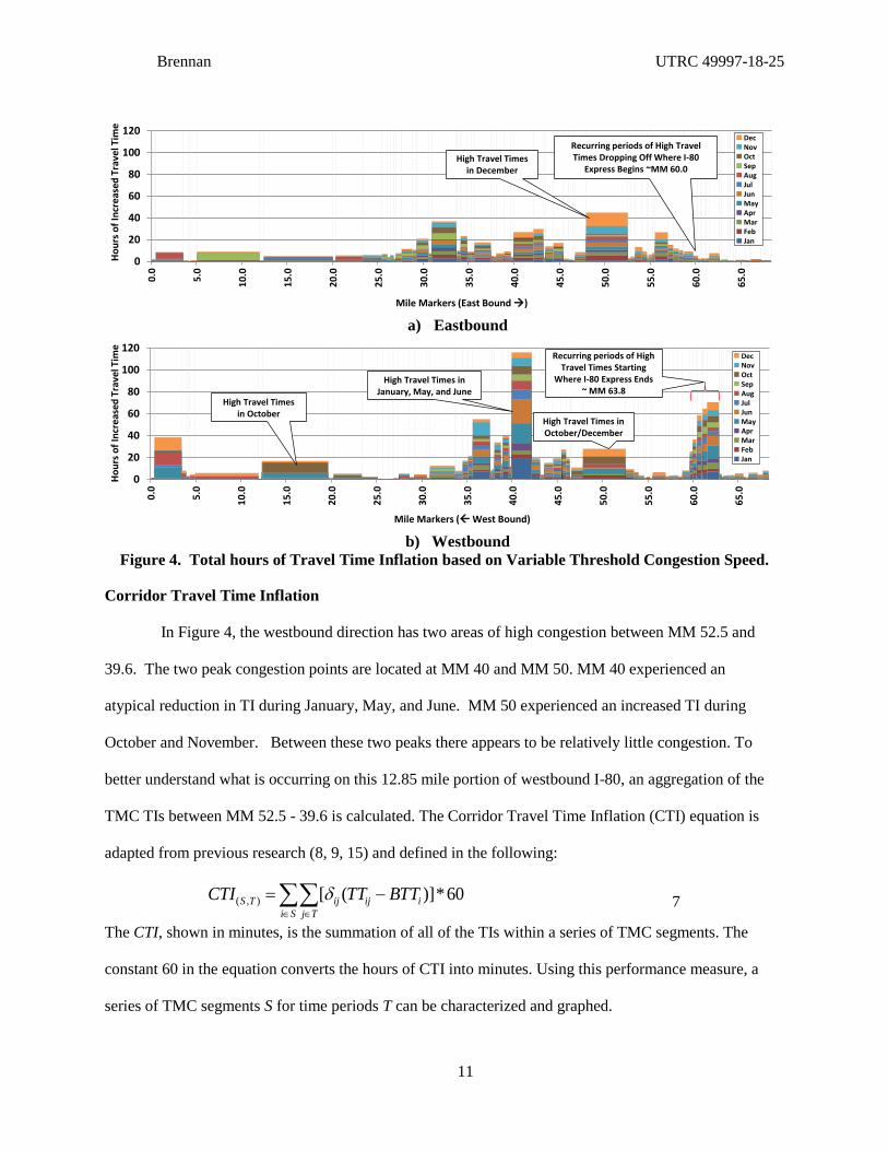
Corridor Travel Time Inflation

In Figure 4, the westbound direction has two areas of high congestion between MM 52.5 and

39.6. The two peak congestion points are located at MM 40 and MM 50. MM 40 experienced an

atypical reduction in TI during January, May, and June. MM 50 experienced an increased TI during

October and November. Between these two peaks there appears to be relatively little congestion. To

better understand what is occurring on this 12.85 mile portion of westbound I-80, an aggregation of the

TMC TIs between MM 52.5 - 39.6 is calculated. The Corridor Travel Time Inflation (CTI) equation is

adapted from previous research (8, 9, 15) and defined in the following:

60*)]([),(

Si Tj

iijijTS BTTTTCTI 7

The CTI, shown in minutes, is the summation of all of the TIs within a series of TMC segments. The

constant 60 in the equation converts the hours of CTI into minutes. Using this performance measure, a

series of TMC segments S for time periods T can be characterized and graphed.

0

20

40

60

80

100

120

0.0

5.0

10.

0

15.

0

20.

0

25.

0

30.

0

35.

0

40.

0

45.

0

50.

0

55.

0

60.

0

65.

0



Ho

urs

of

Incr

ease

d T

rave

l Tim

e

High Travel Times in December

Recurring periods of High Travel Times Dropping Off Where I-80

Express Begins ~MM 60.0

0

20

40

60

80

100

120

0.0

5.0

10.

0

15

.0

20.

0

25.

0

30.

0

35.

0

40.

0

45.

0

50.

0

55.

0

60.

0

65.

0


Mile Markers (West Bound)

Ho

urs

of

Incr

ease

d T

rave

l Tim

e

High Travel Times in January, May, and June

High Travel Times in October

High Travel Times in October/December

Recurring periods of High Travel Times Starting

Where I-80 Express Ends ~ MM 63.8


12

TRAVEL TIME INFLATION VISUALIZTION

The CTI defined in Eq. 7 was applied to the segments between MM 52.5 - 39.6 on westbound I-

80 (Figure 4b). Figure 5 shows a single week (June 9 – 15) illustration of the crowd sourced data to

identify the amount of CTI occurring along the corridor. The longer the TMC the more of an impact it

will have on the CTI. A sample section of one week of data along westbound I-80 from MM 52.8 - 39.6

is shown in Figure 5. In the figure the number of CTI minutes are represented by the color contour

bands (19). The callouts are defined as follows:

Callout i: This line represents the 24-hour time period for the corridor. CTI will appear on this

line and is effectively independent of other days.

Callout ii: This line represents a transitional line from one day to the next. When CTI appears

on this line it could indicate recurring congestion across the corridor. For this case, there is no

recurring congestion at this time.

Callout iii: This small amount of CTI over 5-minutes could represent an incident on June 11

between 1000 and 1345. There is CTI occurring during this time period but it is not observed

on June 10 or June 12, meaning it is isolated to June 11.

Callout iv: This shows the beginning of congestion starting around 1430 on a Friday afternoon.

It is not uncommon to have heavier traffic heading east out of New York on a Friday evening

(Figure 1).

Callout v: The duration of the congested period started at 1430 and ended around 2015,

peaking at 1715. It is noted that on June 15, a Saturday, no congestion delay is observed.

Callout vi: recurring congestion is observed staring June 12 through June 15, with a three day

peak occurring around 1730.

Callout vii: On Jun 13 the congestion duration was less severe when compared to the 14th,

while lasting longer with less intensity when compared to the 12th.


13

Figure 5. One-week example of 24-hour plots of Corridor Travel Time Inflation between

westbound mile markers 52.5 – 39.6.

Visualizing the CTI data in this way allows a temporal representation of congestion. This allows trends

to be seen over the course of a day or week and allows a viewer to understand if the congestion is

recurring or non-recurring. Previously identified in Figure 4b was a high amount of TI during May and

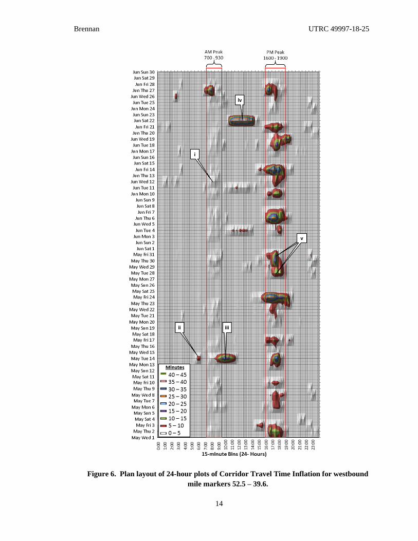
June in the westbound direction of I-80 ending near MM 40. By arranging a series of 1 week graphs, a

two month illustration of the CTI is produced (Figure 6). In the figure the AM and PM peak times can

be observed. Isolated incidents that are outside of the peak travel times, but influenced the overall

congestion (Figure 4) can also be observed. The callouts in Figure 6 are defined as follows:

Callout i: Small, recurring instances of the CTI appear in the AM Peak, heading westbound

away from New York City.

Callout ii: An isolated incident that lasted approximately 45 minutes appears to occur just

before the AM peak.

Callout iii: A more intense incident appears to have occurred in the middle of the AM Peak,

lasting for 2.5 hours.

Callout iv: A major incident lasting from 1000 to 1530 incurred corridor CTI in excess of 40

minutes above the normal threshold for congested travel time.

Callout v: Recurring congestion is observed. Also noted is the decrease in CTI on the

weekends during the PM Peak.

15-minute Bins (24- Hours)

40 – 4535 – 4030 – 3525 – 3020 – 2515 – 2010 – 155 – 100 – 5

Minutes

i iv v viiii

vii

ii


14

Figure 6. Plan layout of 24-hour plots of Corridor Travel Time Inflation for westbound

mile markers 52.5 – 39.6.


15

The two incidents shown in Figure 6 (callouts iii & iv) were major contributors to the TI

observed during May and June in Figure 4b. Viewing the data in series allows recurring congestion to

be viewed with respect to outlier congestion that may adversely impact generalized congestion hour

calculations. Another way to view this data is in an isometric view (Figure 7), where the two incidents

(callouts i & iv) are easily identified. In addition, callout ii shows excessive congestion on the Friday

before Memorial Day weekend, while callout iii shows an incident where the travel time varies every

fifteen minutes. This variation in speed is affiliated with stop and go traffic. Viewing the data in this

perspective provides another means to evaluate the system performance along corridor.


markers 52.5 – 39.6.


40 – 4535 – 4030 – 3525 – 3020 – 2515 – 2010 – 155 – 100 – 5

Minutes

i

ii

iii

iv


16

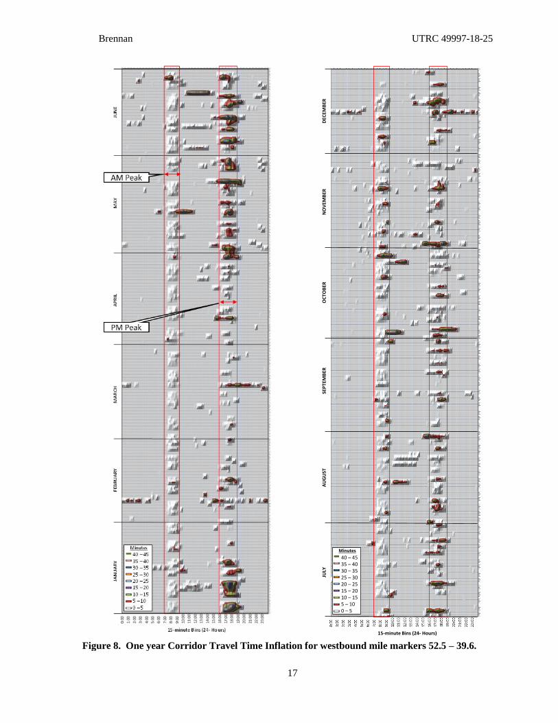
Assembling a series of 24-hour CTI graphs over a one year period provides a method to

evaluate the travel corridor through multiple seasons. The results shown in Figure 8 indicated that the

system appeared to be relatively consistent throughout the year, leading to the conclusion that the travel

time of the corridor is reliable. This does not mean there is no congestion, instead it indicates that the

expectation of a driver leaving New York City at 1630 are reliable for a majority of Fridays throughout

the year. At the beginning of January (Figure 8), there appears to be an unusually high amount of

congestion in the PM Peak period. Viewing the data in an isometric perspective relays a better

understanding of the proportional increase of CTI during the beginning of January (Figure 9 callout i).

In the same figure, callout ii shows a blizzard that occurred on February 8th (18) and callout iii shows an

isolated incident that occurred at the beginning of the PM Peak in April. The individual impacts of each

of the 14 TMC segments that make up the 52.5 to 39.6 westbound corridor during the February 8 storm

are shown in Figure 10. From the figured it can be determined that the smaller the TMC segment, the

less of an impact it has on the total CIT. Conversely, the longer the TMC segment the greater impact I

can have on the CTI.


17

Figure 8. One year Corridor Travel Time Inflation for westbound mile markers 52.5 – 39.6.


JULY

AU

GU

ST

SE

PT

EMB

ER

O

CTO

BER

N

OV

EMB

ER

D

ECEM

BER

PM Peak1600 - 1900

AM Peak700 - 930

40 – 4535 – 4030 – 3525 – 3020 – 2515 – 2010 – 155 – 100 – 5

Minutes


18


markers 52.5 – 39.6.

Figure 10. The contributing values of each of the 14 segments on the CTI values for the I-80

westbound corridor from MM 52.5 – 39.6 during the February 8, 2014 winter storm.


19

Incidents that impact both directions of traffic like weather, rubber necking, construction, and

median crash incidents can be identified when both the eastbound and westbound direction CTIs are

calculated and graphed. In Figure 11, a six month view of the CTI maps for both direction of I-80 are

shown. The AM and PM peak times are labeled on the maps and are relatively consistent in each

direction. Isolated traffic incidents are expected to appear in one direction and not the other, while

weather events and major incidents are expected to impact both directions. On March 18th a late season

winter storm (18) occurred (callout i) that impacted both directions of I-80. The major winter storm

identified in Figure 9 (callout ii) appears in both directions of Figure 11 (callout ii). The use of the

isometric CTI maps provide a definitive means to effectively relay the proportional increases in travel

time incurred along a corridor. These types of illustrations provide a simplistic method to convey

problem areas to an agency when making capital infrastructure investment decisions.


20

Figure 11. Side by side layout of Corridor Travel Time Inflation plot for eastbound and for

westbound I-80 traffic between mile markers 52.5 – 39.6.


21

AGGREGATED SEGMENT TRAVEL TIME

By aggregating the TI values over time, a representation of the relative congestion intensity can

be evaluated. The results of the travel time inflation performance measure are shown in Figure 4, where

thicker bands indicate increased travel time. This can be observed in Figure 4a and Figure 4b where the

eastbound TI is higher in December. For the eastbound direction (Figure 4a), as traffic approached the I-

80 expressway into New York City, the TI values decreased. This indicates a reduction in travel time as

vehicles depart local I-80 to enter the I-80 expressway (Figure 1). In the westbound direction (Figure

4b) the opposite effect occurs. The TI increased when the I-80 expressway ends, but decreased over the

next 4 miles. In Figure 4 the I-80 congestion hotspots are identified by a pronounced increase in TI. It is

expected that most of the TI occurs during the AM and PM peak travel times, but this information

cannot be interpreted from the graph.

a) Eastbound

b) Westbound

Figure 12. Total hours of Travel Time Inflation based on Variable Threshold Congestion Speed.

From Figure 4, it can be observed that the westbound direction has two areas of high congestion

between MM 52.5 and 39.6. The two peak congestion points are located at MM 40 and MM 50. MM 40

0

20

40

60

80

100

120

0.0

5.0

10

.0

15

.0

20

.0

25

.0

30

.0

35

.0

40

.0

45

.0

50

.0

55

.0

60

.0

65

.0



Ho

urs

of

Incr

eas

ed T

rave

l Tim

e

High Travel Times in December

Recurring periods of High Travel Times Dropping Off Where I-80

Express Begins ~MM 60.0

0

20

40

60

80

100

120

0.0

5.0

10.

0

15.

0

20.

0

25.

0

30.

0

35.

0

40.

0

45.

0

50.

0

55.

0

60.

0

65.

0


Mile Markers (West Bound)

Ho

urs

of

Incr

ease

d T

rave

l Tim

e

High Travel Times in January, May, and June

High Travel Times in October

High Travel Times in October/December

Recurring periods of High Travel Times Starting

Where I-80 Express Ends ~ MM 63.8


22

experienced an atypical reduction in TI during January, May, and June. MM 50 experienced an

increased TI during October and November. Between these two peaks there appears to be relatively

little congestion, leading to the conclusion that the segments between the two mile markers can be

grouped together to better understand what is occurring on this 12.85 mile portion of westbound I-80.

An aggregation of the TMC TIs between MM 52.5 - 39.6 using the corridor travel time inflation (CTI)

equation, defined in previous research (1):

Statistical evaluation of travel corridors

Although the approximate location of a change in increased travel times could be qualitatively

observed in Figure 12, the appropriate groups of statistically similar segments cannot be determine

directly from this graph. The problem with using just the TI as a performance measures is that it

inherently reflects greater amounts of congestion for longer TMC segments. This makes it difficult to

statistically compare the congestion characteristics of adjacent TMCs. Normalizing the increase in travel

time with the Percent increases in Mean Travel time (PMTT) performance measure accounts for

differences in TMC lengths. The PMTT is shown in the following equation:

i

iij

BTT

TIPMTT 8

where PMTTij is the percent total Travel Time Inflation compared to the base travel time for a TMC

segment i for a 15-minute bin time period j within a time frame defined by the analyst. A general

representation of this performance measure is shown in Figure 13 where the relative increases in PMTT

are plotted against the months of the year in 2013. Each mile marker (MM) is represented by a line with

the top most line being the western most segment. With reference to the graph, segments with similarly

spaced horizontal lines indicate a potential to consider these segments with similar congestion

characteristics. The graph is plotted with respect to the months of the year to show the variation in this

value during different types of seasons. A similar plot is shown in Figure 14, where each line represents a


23

month of the year plotted along the entire corridor. The PMTT during the AM Peak is shown in Figure

14a, while the aggregated increases are shown in Figure 14b.

Figure 13. Relative differences between the mean values of the average percent increase in travel

time per month.

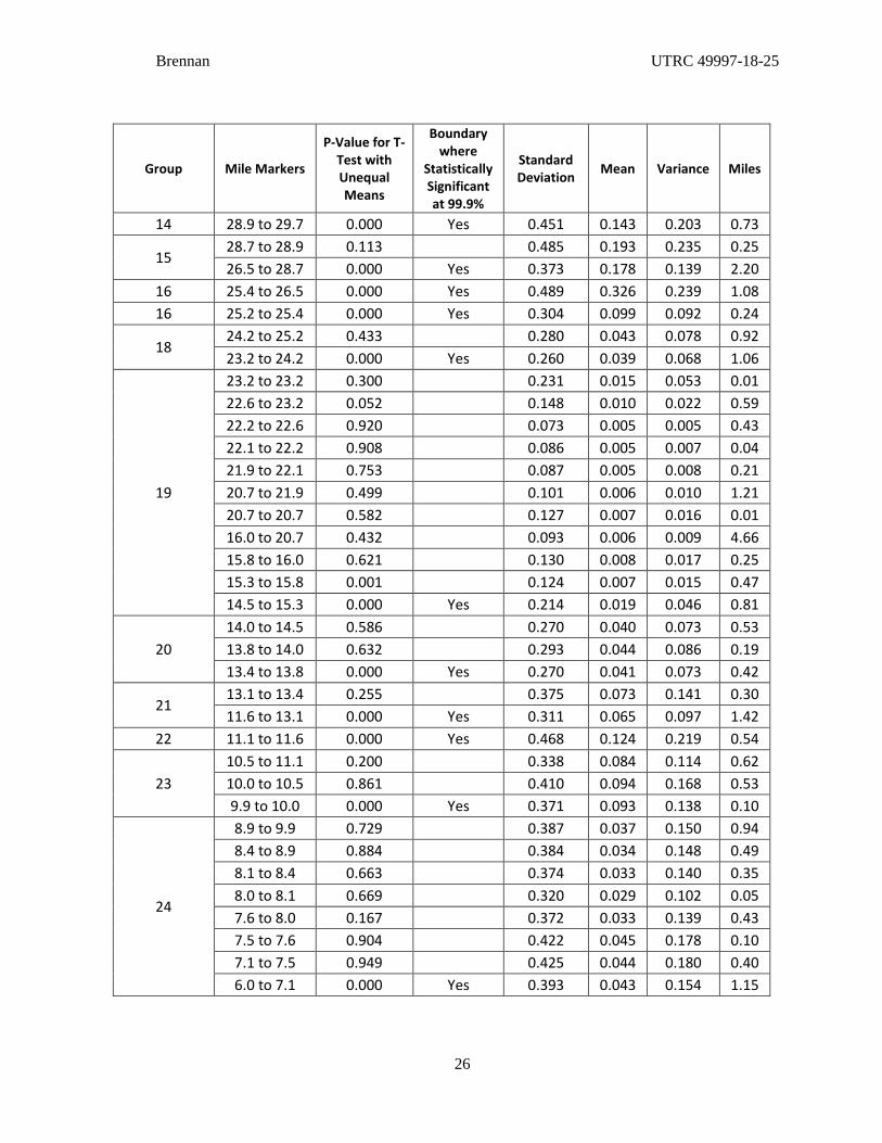
An F-Test was performed on the background data to determine if the travel time mean values

were near equal. From the F-Test it was determined that no highway segment had travel time means

that were statistically similar. This result indicated that in order to perform at T-Test, an assumption

that the mean values are unequal had to be made. The t-test was applied to each adjacent segment at a

99.9% confidence interval to minimize the number of groups. The results of the t-test with the

respective p-values are shown in Table 3. The T-Test results indicate 25 distinct groups of I-80 which

have travel time reliabilities in the eastbound direction during the AM Peak travel time period.


24

a. Average percent increase in Travel Time per Month

b. Aggregated average percent increase in Travel Time per Month

Figure 14. AM Peak eastbound differences between the mean values of the average percent

increase in travel time I-80

0.00

0.10

0.20

0.30

0.40

0.50

0.60

0.70

0.80

68

.5 t

o 6

8.6

68

.2 t

o 6

8.3

65

.1 t

o 6

8.1

64

.5 t

o 6

5.1

64.

3 t

o 6

4.3

56

.7 t

o 6

3.6

48

.6 t

o 5

6.2

45.

3 t

o 4

8.3

42

.6 t

o 4

3.2

41

.8 t

o 4

2.3

41

.0 t

o 4

1.6

39

.3 t

o 3

9.9

37

.7 t

o 3

8.1

34

.9 t

o 3

5.0

33

.7 t

o 3

4.5

33.

0 t

o 3

3.4

30

.8 t

o 3

1.2

29

.7 t

o 3

0.6

28

.9 t

o 2

9.7

26

.5 t

o 2

8.7

25

.2 t

o 2

5.4

23

.2 t

o 2

4.2

22

.6 t

o 2

3.2

22.

1 t

o 2

2.2

20

.7 t

o 2

1.9

16

.0 t

o 2

0.7

15

.3 t

o 1

5.8

14

.0 t

o 1

4.5

13

.4 t

o 1

3.8

11

.6 t

o 1

3.1

10

.5 t

o 1

1.1

9.9

to

10

.0

8.4

to

8.9

8.0

to

8.1

7.5

to

7.6

6.0

to

7.1

5.1

to

5.8

4.4

to

4.8

3.1

to

4.2

2.5

to

2.7

0.9

to

1.4

0.0

to

0.3

1

2

3

4

5

6

7

8

9

10

11

12

Jan

Feb

Mar

Apr

Jun

Jul

Aug

Sep

Oct

Nov

Dec

Ave

rage

% In

cre

ase

in T

rave

l Tim

e P

er

Mo

nth

Mile Markers on I-80

0.00

0.50

1.00

1.50

2.00

2.50

3.00

3.50

4.00

4.50

5.00

68

.5 t

o 6

8.6

68

.2 t

o 6

8.3

65

.1 t

o 6

8.1

64

.5 t

o 6

5.1

64.

3 t

o 6

4.3

56

.7 t

o 6

3.6

48

.6 t

o 5

6.2

45.

3 t

o 4

8.3

42

.6 t

o 4

3.2

41

.8 t

o 4

2.3

41

.0 t

o 4

1.6

39

.3 t

o 3

9.9

37

.7 t

o 3

8.1

34

.9 t

o 3

5.0

33

.7 t

o 3

4.5

33.

0 t

o 3

3.4

30

.8 t

o 3

1.2

29

.7 t

o 3

0.6

28

.9 t

o 2

9.7

26

.5 t

o 2

8.7

25

.2 t

o 2

5.4

23

.2 t

o 2

4.2

22

.6 t

o 2

3.2

22.

1 t

o 2

2.2

20

.7 t

o 2

1.9

16

.0 t

o 2

0.7

15

.3 t

o 1

5.8

14

.0 t

o 1

4.5

13

.4 t

o 1

3.8

11

.6 t

o 1

3.1

10

.5 t

o 1

1.1

9.9

to

10

.0

8.4

to

8.9

8.0

to

8.1

7.5

to

7.6

6.0

to

7.1

5.1

to

5.8

4.4

to

4.8

3.1

to

4.2

2.5

to

2.7

0.9

to

1.4

0.0

to

0.3

0.00

0.10

0.20

0.30

0.40

0.50

0.60

0.70

0.80

68

.5 t

o 6

8.6

68

.2 t

o 6

8.3

65

.1 t

o 6

8.1

64

.5 t

o 6

5.1

64.

3 t

o 6

4.3

56

.7 t

o 6

3.6

48

.6 t

o 5

6.2

45.

3 t

o 4

8.3

42

.6 t

o 4

3.2

41

.8 t

o 4

2.3

41

.0 t

o 4

1.6

39

.3 t

o 3

9.9

37

.7 t

o 3

8.1

34

.9 t

o 3

5.0

33

.7 t

o 3

4.5

33.

0 t

o 3

3.4

30

.8 t

o 3

1.2

29

.7 t

o 3

0.6

28

.9 t

o 2

9.7

26

.5 t

o 2

8.7

25

.2 t

o 2

5.4

23

.2 t

o 2

4.2

22

.6 t

o 2

3.2

22.

1 t

o 2

2.2

20

.7 t

o 2

1.9

16

.0 t

o 2

0.7

15

.3 t

o 1

5.8

14

.0 t

o 1

4.5

13

.4 t

o 1

3.8

11

.6 t

o 1

3.1

10

.5 t

o 1

1.1

9.9

to

10

.0

8.4

to

8.9

8.0

to

8.1

7.5

to

7.6

6.0

to

7.1

5.1

to

5.8

4.4

to

4.8

3.1

to

4.2

2.5

to

2.7

0.9

to

1.4

0.0

to

0.3

1

2

3

4

5

6

7

8

9

10

11

12

Jan

Feb

Mar

Apr

Jun

Jul

Aug

Sep

Oct

Nov

Dec

Re

lati

ve A

vera

ge %

Incr

eas

e in

Tra

vel T

ime

Pe

r M

on

th

Mile Markers on I-80


25

Table 3. T-Test grouping of 83 eastbound AM Peak travel time highway segments along I-80, 2013

Group Mile Markers

P-Value for T-Test with Unequal Means

Boundary where

Statistically Significant at

99.9%

Standard Deviation

Mean Variance Miles

1

68.5 to 68.6 0.890 0.237 0.012 0.056 0.11

68.3 to 68.5 0.993 0.245 0.013 0.060 0.22

68.2 to 68.3 0.730 0.244 0.013 0.059 0.09

68.1 to 68.2 0.001 Yes 0.211 0.011 0.045 0.04

2

65.1 to 68.1 0.129 0.007 0.000 0.000 3.00

65.1 to 65.1 0.342 0.001 0.000 0.000 0.06

64.5 to 65.1 0.249 0.002 0.000 0.000 0.58

64.3 to 64.5 0.195 0.010 0.000 0.000 0.19

64.3 to 64.3 0.034 0.014 0.001 0.000 0.03

63.6 to 64.3 0.146 0.004 0.000 0.000 0.69

56.7 to 63.6 0.317 0.000 0.000 0.000 6.92

56.2 to 56.7 0.317 0.002 0.000 0.000 0.48

48.6 to 56.2 0.082 0.000 0.000 0.000 7.60

48.3 to 48.6 0.432 0.024 0.001 0.001 0.28

45.3 to 48.3 0.000 Yes 0.031 0.001 0.001 3.01

3 43.2 to 45.3 0.000 Yes 0.235 0.017 0.055 2.11

4

42.6 to 43.2 0.402 0.646 0.097 0.417 0.57

42.3 to 42.6 0.153 0.618 0.109 0.382 0.30

41.8 to 42.3 0.981 0.475 0.092 0.226 0.46

41.6 to 41.8 0.033 0.439 0.091 0.192 0.20

41.0 to 41.6 0.669 0.477 0.113 0.228 0.64

39.9 to 41.0 0.000 Yes 0.424 0.109 0.180 1.14

5

39.3 to 39.9 0.036 0.732 0.235 0.535 0.52

38.1 to 39.3 0.604 0.572 0.204 0.328 1.22

37.7 to 38.1 0.000 Yes 0.600 0.211 0.359 0.41

6 35.0 to 37.7 0.000 Yes 0.486 0.159 0.236 2.76

7 34.9 to 35.0 0.004 0.667 0.248 0.445 0.03

34.5 to 34.9 0.000 Yes 0.755 0.293 0.570 0.42

8 33.7 to 34.5 0.000 Yes 0.835 0.381 0.697 0.75

9 33.4 to 33.7 0.000 Yes 0.656 0.315 0.431 0.34

10 33.0 to 33.4 0.000 Yes 0.538 0.236 0.289 0.46

11 31.2 to 33.0 0.000 Yes 0.382 0.124 0.146 1.76

12 30.8 to 31.2 0.133 0.551 0.191 0.304 0.35

30.6 to 30.8 0.000 Yes 0.507 0.209 0.257 0.28

13 29.7 to 30.6 0.582 0.293 0.088 0.086 0.87

29.7 to 29.7 0.000 Yes 0.331 0.084 0.110 0.03


26

Group Mile Markers


Boundary where

Statistically Significant at 99.9%

Standard Deviation

Mean Variance Miles

14 28.9 to 29.7 0.000 Yes 0.451 0.143 0.203 0.73

15 28.7 to 28.9 0.113 0.485 0.193 0.235 0.25

26.5 to 28.7 0.000 Yes 0.373 0.178 0.139 2.20

16 25.4 to 26.5 0.000 Yes 0.489 0.326 0.239 1.08

16 25.2 to 25.4 0.000 Yes 0.304 0.099 0.092 0.24

18 24.2 to 25.2 0.433 0.280 0.043 0.078 0.92

23.2 to 24.2 0.000 Yes 0.260 0.039 0.068 1.06

19

23.2 to 23.2 0.300 0.231 0.015 0.053 0.01

22.6 to 23.2 0.052 0.148 0.010 0.022 0.59

22.2 to 22.6 0.920 0.073 0.005 0.005 0.43

22.1 to 22.2 0.908 0.086 0.005 0.007 0.04

21.9 to 22.1 0.753 0.087 0.005 0.008 0.21

20.7 to 21.9 0.499 0.101 0.006 0.010 1.21

20.7 to 20.7 0.582 0.127 0.007 0.016 0.01

16.0 to 20.7 0.432 0.093 0.006 0.009 4.66

15.8 to 16.0 0.621 0.130 0.008 0.017 0.25

15.3 to 15.8 0.001 0.124 0.007 0.015 0.47

14.5 to 15.3 0.000 Yes 0.214 0.019 0.046 0.81

20

14.0 to 14.5 0.586 0.270 0.040 0.073 0.53

13.8 to 14.0 0.632 0.293 0.044 0.086 0.19

13.4 to 13.8 0.000 Yes 0.270 0.041 0.073 0.42

21 13.1 to 13.4 0.255 0.375 0.073 0.141 0.30

11.6 to 13.1 0.000 Yes 0.311 0.065 0.097 1.42

22 11.1 to 11.6 0.000 Yes 0.468 0.124 0.219 0.54

23

10.5 to 11.1 0.200 0.338 0.084 0.114 0.62

10.0 to 10.5 0.861 0.410 0.094 0.168 0.53

9.9 to 10.0 0.000 Yes 0.371 0.093 0.138 0.10

24

8.9 to 9.9 0.729 0.387 0.037 0.150 0.94

8.4 to 8.9 0.884 0.384 0.034 0.148 0.49

8.1 to 8.4 0.663 0.374 0.033 0.140 0.35

8.0 to 8.1 0.669 0.320 0.029 0.102 0.05

7.6 to 8.0 0.167 0.372 0.033 0.139 0.43

7.5 to 7.6 0.904 0.422 0.045 0.178 0.10

7.1 to 7.5 0.949 0.425 0.044 0.180 0.40

6.0 to 7.1 0.000 Yes 0.393 0.043 0.154 1.15


27

Group Mile Markers


Boundary where

Statistically Significant at 99.9%

Standard Deviation

Mean Variance Miles

25

5.8 to 6.0 0.544 0.208 0.014 0.043 0.18

5.1 to 5.8 0.542 0.244 0.011 0.060 0.71

4.8 to 5.1 0.008 0.185 0.008 0.034 0.23

4.4 to 4.8 0.667 0.021 0.001 0.000 0.47

4.2 to 4.4 0.672 0.022 0.000 0.001 0.19

3.1 to 4.2 0.587 0.010 0.000 0.000 1.10

2.7 to 3.1 0.975 0.032 0.001 0.001 0.35

2.5 to 2.7 0.926 0.034 0.001 0.001 0.27

1.4 to 2.5 0.216 0.031 0.001 0.001 1.03

0.9 to 1.4 0.554 0.001 0.000 0.000 0.52

0.3 to 0.9 0.002 0.002 0.000 0.000 0.65

0.0 to 0.3 NA NA 0.062 0.003 0.004 0.26

Table 4. ANOVA analysis for six segments between MM 39.9 – 43.2

ANOVA

Source of Variation SS df MS F P-value F crit

Segments 1.966228 5 0.393246 1.458947 0.199672 4.104525

CONCLUSION

As probe vehicle data become more reliable, local, state, regional, and national standards need

to be established to leverage this data for better congestion management practices. This report proposed

a scalable means to characterize congestion called that Travel Time Inflation (TI) performance measure.

This performance measure was applied to 68 miles of Interstate-80 in New Jersey. By measuring

anonymous probe vehicle speeds along a highway, a threshold to determine when congestion occurs can

be established. The TI performance measure accounts for speed variation along a corridor which impact

free flow speeds and travel times. Instead of applying a set value, a variable congestion threshold is

calculated along a predetermine series of roadway segments called Traffic Message Channels (TMCs)


28

or Traffic Message Channel (TMC). By establishing a base congestion measure for each TMC segment

a more accurate measurement of the increased travel times that accounts for different roadway

conditions is established. This is particularly important for a corridor like I-80 that experiences a

variety of terrain types, vehicle volumes, and population densities. Because the TI cannot demonstrate

the time of day when congestion is occurring, a Corridor Travel Time Inflation (CTI) was established to

visualize congestion periods on an hourly and daily basis. Although it is not practical to eliminate all

congestion, having a better means to visually document congestion based on individual TMC attributes

provides a better method of locating and ultimately managing congestion occurrences.

The problem with using just the TI as a performance measures is that it inherently reflects

greater amounts of congestion for longer TMC segments. This makes it difficult to directly compare the

congestion characteristics of adjacent TMCs. By normalizing the increase in travel time with the

Percent increases in Mean Travel time (PMTT) performance measure, a statistical comparison can be

made between adjacent TMCs. A T-Test analysis was performed on the PMTT calculated between

adjacent TMCs. The results indicate that of the available TMC segments along the eastbound portion of

I-80, there were 25 groups of TMCs that had similar statistical travel time reliabilities. An ANOVA test

was applied, and showed that in some instances the results agreed with the T-Test. However, further

research will be conducted to compare different statistical methods to group TMC segments and to to

evaluate the consistency of the groups during PM Peak travel times, seasonal travel, and winter weather

travel.

The visualization techniques proposed in the report are an intuitive way to relay the congestion

conditions along a corridor to any person who is making decisions regarding capital improvements,

construction scheduling, and other roadway management tasks. By consolidating a very large number

of speed records for an entire year (Figure 8) into a single picture, a more useable representation of the

corridor’s performance is developed. Furthermore, by viewing the data in an isometric view (Figure 7

and Figure 9), a better understanding of the magnitude of congestion can be interpreted. The graphical

representation of the data also provides a more practical way to archive the data, which can be


29

referenced in the future by analysts who want to determine how long term capital improvements or

policy changes impact a corridor. Ultimately the goal of this type of research is to reduce the overall

congestion through better management practices. With a better understanding of where, when, and over

what distances traffic congestion is occurring, better management practices and policies can be

established.


30

REFERENCES

1. Brennan, T. M., S.M., Remias and L. Marini, “Performance Measures to Characterize Corridor Travel

Time Delay Based on Probe Vehicle Data”, Transportation Research Board, Paper number 15-0167,

Washington, DC, (2015) IN PRESS.

2. Brennan, T. M., Hainen, A. M.., and Remias,. (2015). Characterizing Directional Corridors Based

On Probe Vehicle Data. ITS 23rd World Congress Bordeaux, France (accepted)

3. FHWA, “MAP-21 Moving Ahead for Progress in the 21st Century Act” July 2012

4. ASCE. (2013). Report Card for America’s Infrastructure,

http://www.infrastructurereportcard.org/roads/ (July 9, 2014)

5. Lomax, T., D. Shrank, B. Eiselee. 2012 Annual Urban Mobility Report. College Station, Texas; The

Texas A&M University System, Texas A& M Transportation Institute, 2012.

6. Lomax, T., D. Shrank, B. Eiselee. 2011 Urban Mobility Report Powered by INRIX Traffic Data.

College Station, Texas; The Texas A&M University System, Texas A& M Transportation Institute,

2011.

7. Remias S, Brennan T, Grimmer G, Cox E, Horton D, Bullock D. 2011 Indiana Interstate Mobility

Report - Full Version. West Lafayette, Indiana: Purdue University, Indiana Mobility Reports; 2012.

Report No.: ISBN: 978-1-62260-209-4.

8. Remias S, Brennan T, Day C, Summers H, Cox E, Horton D, Bullock D. 2012 Indiana Mobility

Report - Full Version. West Lafayette, Indiana: Purdue University, Indiana Mobility Reports; 2013.

Report No.: ISBN: 978-1-62260-257-5.

9. Remias, Stephen, M., T.M. Brennan, C.M. Day, H.T. Summers, D.K. Horton, E.D. Cox and D.M.

Bullock, “Spatially Referenced Probe Data Performance Measures for Infrastructure Investment

Decision Makers,” Submitted to Transportation Research Board, August 1, 2013, Paper No. 14-

1062.

10. Maryland Department of Transportation, “2012 Maryland State Highway Mobility Report,” July

2012.

11. California Department of Transportation, “Mobility Performance Report 2009”, February 2011.

12. Washington State Department of Transportation, “The 2012 Congestion Report,” August 2012.

13. Haghani, A., M. Hamdi, K.F. Sadabadi, “I-95 Corridor coalition vehicle probe project: validation of

Inrix data July-September 2008-Final Report,” I-95 Corridor Coalition. January 2009.

14. Brennan Jr., T.M., S.M. Remias, D.K. Horton, and D.M. Bullock, “Probe Vehicle Based Statewide

Mobility Performance Measures for Decision Makers,” Transportation Research Record: Journal of

the Transportation Research Board, 2338(1), 78-90, 2013

15. Brennan, T. M., Day, C.M., Remias, G.M. Horton, D.K., Cox, E.D., Bullock, D. M. (2014).

Alternative Performance Measures and Weighting for Quantifying Spatial and Temporal Congestion

using Probe Data. ITS 21st World Congress


31

16. Christidis, P., & Rivas, J. N. I. (2012). Measuring Road Congestion (No. JRC69961). Institute for

Prospective and Technological Studies, Joint Research Centre, Seville, Spain.

17. Lomax, T., et al. "NCHRP report 398: quantifying congestion." Transportation Research

Board, National Research Council, Washington, DC. Final report (1997).

18. http://www.erh.noaa.gov/okx/StormEvents/storm02082013.html (July 10, 2014)

19. Brennan, T.M, D.M. Bullock, “Regional Travel Time Reliability” The 5th International Symposium

on Transportation Network Reliability (INSTR2012), 18-19 December 2012, Hong Kong.

Univ

ersi

ty T

rans

port

atio

n Re

sear

ch C

ente

r - R

egio

n 2

Fund

ed b

y the

U.S.

Dep

artm

ent o

f Tra

nspo

rtat

ion

Region 2 - University Transportation Research Center

The City College of New YorkMarshak Hall, Suite 910

160 Convent AvenueNew York, NY 10031Tel: (212) 650-8050Fax: (212) 650-8374

Website: www.utrc2.org

finalreport - university transportation research center measures to characterize ... negotiation...

Documents