Final Report TO THE

NATIONAL OCEANIC & ATMOSPHERIC ADMINISTRATION (NOAA)Joint Hurricane Testbed (JHT) Program

For theAtlantic Oceanographic and Meteorological Laboratory

4301 Rickenbacker CausewayMiami, Florida 33149

Project: Drag Coefficient Distribution and Wind Speed Dependence in Tropical Cyclones

Principal Investigator: Mark D Powell NOAA/AOML

PERFORMANCE PERIOD : April 1, 2005 – April 1 , 2007

DATE: April 18, 2006

1

Drag Coefficient Distribution and Wind Speed Dependence in Tropical Cyclones

Principal Investigator:

Mark D. Powell NOAA Hurricane Research DivisionCollaborator: Isaac Ginis, University of Rhode IslandGraduate School of Oceanographyiginis@gso.uri.edu

Executive Summary

A total of 2664 processed GPS sonde profiles from the period 1997-2005 were loaded into a re-lational database. A database schema was designed and an interactive graphical query interface was built utilizing commercial database management software (Oracle 9i). After filtering the pro-files to those within 2-200 km of the tropical cyclone center with MBL (mean (< 500m) bound-ary layer) wind speeds > 20 m s-1, 1270 sonde profiles were available for analysis for MBL wind speed groups of 20-29, 30-39, 40-49, 50-59, 60-69, and 70-79 m s-1. Roughness length, friction velocity, drag coefficient, and 10 m level neutral stability wind speed (U10) were diagnosed in each MBL group using the profile method. The drag coefficient increases linearly with U10

reaching a maximum of 2 x 10-3 at a wind speed of 41 m s-1, thereafter it decreases with increas-ing wind speed to a minimum of 0.6 x 10-3 at U10 of 61 m s-1. When broken down into radial groups of R<= 30 km and R> 30 km, the profiles within 30 km of the center show Cd values that display little variation of Cd with wind speed and smaller values of Cd near 1 x 10-3, consistent with Donelan’s continuous breaking hypothesis. Profiles outside of 30 km show the behavior described earlier (initial increase followed by a decrease). After dividing the R> 30 km profiles into storm relative azimuth sectors, the increase-then-decrease behavior was found to be con-fined to the front left sector where the winds flow across the primary swells. These results have bearing on the current wave-roughness interaction parameterizations being considered for the HWRF model.

2

1. Introduction

Sea surface momentum flux or stress (

€

τ ) in numerical weather prediction of tropical cyclones is modeled using the "bulk aerodynamic method" as:

€

τ = ρCDU102 = ρu *2 (1)

based on a drag coefficient (CD) and the 10 m wind speed (U10) which varies logarithmically

with height as described by the "log law" :

€

U10 =U *kLn z

zo

(2)

where U* is the friction velocity, k is a constant, z is the height. The aerodynamic roughness length (Zo) is typically modeled through the Charnock (1955) relationship, which implies that the aerodynamic roughness of the sea surface increases with wind speed according to:

€

Zo =αu *2

g (3)

where g is the gravitational constant. The Charnock coefficient,

€

α in this expression takes on values ranging from 0.015 to 0.035.

The surface momentum flux is therefore governed by the drag or friction at the sea surface which in turn depends on a roughness which is parameterized as increasing with increasing wind speed. Measurements support this parameterization only up to wind speeds of ~28 m/s. For higher wind speeds the roughness dependence is extrapolated e.g. Large and Pond (1981). The surface enthalpy flux is also modeled using the bulk aerodynamic method and employs an enthalpy ex-change coefficient that is dependent on CD. According to the theory of Emanuel (1995), a hurri-

cane is only maintained if kinetic energy is supplied by oceanic heat sources at a rate exceeding dissipation, suggesting a ratio of enthalpy exchange coefficient (CE) to CD ranging from 1.2 to

1.5 for mature hurricanes. At extreme wind speeds > 50 m/s, the typical extrapolations of wind speed dependent drag coefficients found in most models cause kinetic energy to be destroyed too rapidly to sustain a hurricane (Donelan et al., 2004).

In Powell et al., (2003), hereafter "PVR", analysis of mean profiles documented a logarithmic change of wind speed with height, suggesting the applicability of surface layer similarity in con-ditions associated with MBL winds up to 70 m/s. Using the “Profile Method”, a fit of the pro-files provided information on the surface stress or friction velocity (slope) and roughness (inter-

3

cept) as a function of wind speed. The basis for the Profile method used by PVR method is that each sonde profile is a realization or snap shot of tropical cyclone conditions. By organizing numerous realizations as a function of wind speed, the ergodic hypothesis (Panofsky and Dutton 1984) is invoked to consider each profile as an instance from an ensemble of profile samples in nearly identical conditions. The primary feature controlling the turbulence in these conditions is the ocean surface roughness and this quantity is dependent on the wind stress and sea state, hence the organization by wind speed. The profiles are organized by the "mean boundary layer" wind speed, defined as the average of all values below 500 m. Profiles are filtered to remove under-sampled flow (turbulent eddies, convective- and swell-related features) and noise due to satellite switching. Averaging the profiles removes larger scale convective features such as tran-sient wind maxima or minima and provides information on the mean state and how it changes with the wind forcing.

PVR analyzed 331 GPS sondes dropped in 15 storms from 1997-1999. This analysis determined a leveling off of the surface stress and drag coefficient in wind speeds > 34 m/s and a reduction in roughness length. This was the first time that measurements of drag coefficient were made in winds > 28 m/s.

The PVR findings have recently been corroborated by wind flume experiments (Donelan et al., 2004) and are already influencing model parameterizations of momentum flux in the hurricane boundary layer ( Andreas 2004, Moon et al., 2004, Wang and Wu 2004). Moon et al., 2004 reports significant improvement of momentum flux parameterization using the WAVEWATCH wave model coupled with a new wave-wind model. Their model estimates of the surface rough-ness and drag coefficient in hurricanes compare favorably with PVR and the wave spectrum variation of Wright et al., 2001. The Moon et al., 2004 study suggested that higher and more developed waves produce higher sea drag in the right-front quadrant and lower and younger waves produce lower sea drag in the rear-left quadrant. This asymmetry increased with hurricane translation speed. The group at University of Miami lead by Mark Donelan and Shuyi Chen are also investigating wave dependent momentum flux parameterizations. Wang and Wu (2004) commented on the PVR work in a review article: "This breakthrough can lead to reduction of the uncertainties in the calculation of surface fluxes, thus improving TC intensity forecasts by nu-merical weather prediction models."

The recent CBLAST experiments, together with several additional years of research flights and operational reconnaissance have increased the number of high wind GPS sonde profiles to > 1200. Numerous sonde profiles are unwieldy for analysis with spreadsheet-type tools but ideal for a modern object-relational database. The large number of sondes will make possible more accurate ensemble mean profiles, as well as examination of how the mean profiles change with storm-relative quadrant. The intensive CBLAST investigations of 2003 Hurricanes Fabian and Isabel, together with experiments conducted in Hurricanes Frances, Ivan, and Jeanne of 2004 , and intensive sampling of 2005 Hurricanes Katrina, Rita, and Wilma, provide a wealth of high wind GPS sonde profile measurements to extend the work of PVR.

4

In particular, observational determination of the spatial distribution of roughness relative to the hurricane center to account for azimuthal variation of wave age and steepness as a function of wind speed will provide a data set for validating the current model parameterizations and devel-oping new ones. To evaluate the effect of sea state, which varies in azimuth because of the varia-tion in swell characteristics relative to the wind, a larger (than PVR) data set is needed, ideally containing ~150 profiles for a given MBL grouping. The GPS sonde data through 2005 provide sufficient profiles to study the azimuthal variation of surface stress and roughness.

Current models used to predict hurricane track and intensity use methods similar to (1). For example, an early version of the coupled GFDL model Bender et al., (1993) uses (3) with a con-stant of 0.0185. A new coupled version of GFDL model uses a coupled wave-wind model in which

€

α increases with the input wave age and the surface wind speed. The planned HWRF model has a modular design that allows using different boundary layer physics packages. Care-ful testing will determine the final package used in the operational version of the model but re-gardless of the version, proper modeling of the surface momentum flux will need to account for the observed change in roughness as the wind speed increases, and wave interactions with the wind that cause azimuthal variation in the roughness. In addition, it is expected that our results will also be valuable for wave and storm surge modeling with the coupled HWRF/ocean/ wave model. The project is applied towards JHT numerical weather prediction priorities EMC-1 and EMC-2.

2. Sonde database

a. Inventory

Not all launched GPS sondes undergo post processing. Many undergo onboard processing to enable a coded transmission of profile information from the aircraft but do not receive further post-flight processing. Post-flight processing uses the EditSonde software written by James Franklin (Franklin 1997) and is a time intensive activity involving an experienced analyst. Al-ternative processing software (ASPEN) is available from NCAR but recent experiments by SIm Aberson and Michael Black of HRD indicate that the Editsonde software is superior for research purposes. An inventory was assembled to allow the investigators to determine how many sondes have been launched for each research or recon flight, how many were transmitted, and how many were post processed. As indicated in Table 1, based on GPS sonde launch logs from numerous aircraft missions, 6148 sondes have been launched since 1997. Of these, 2343 post-processed sondes have been loaded into the database as of this report date.

From a total of 42 tropical cyclones since 1997, 460 storm track files were constructed using wind center fixes from the 550 flights in the inventory. The track files allow spline fits to the change in storm latitude and longitude with time, allowing calculation of the storm-relative radial and azimuthal coordinates of the sonde splash locations as well as the radial and tangential wind components. Sondes dropped during NOAA G-4 flights are also contained in the database and

5

must use storm track files created from other flights that took place during the time of a G-4 flight. At the date of this report, 629 sondes (generally dropped in peripheral locations by the NOAA G-4 jet aircraft) await storm track information before they can be loaded into the data-base.

One of the more time consuming aspects of the project was to integrate a database of flight-level observations organized by radial flight legs. A scaled radial coordinate could be determined by using the maximum flight-level wind speed on the particular radial leg on which a sonde has been launched. The flight-level database could then be “joined” to the sonde database to assign each sonde entry a scaled radial coordinate based on azimuthal proximity to to radial flight legs. Problems were encountered in developing logic to objectively determine radial legs from a par-ticular flight. Radial flight-level leg data were joined for sondes the 40-49 m s-1 MBL group but relevant Rmax could only be determined for 180 of the 237 sondes in the group. Work continues to improve the objective Rmax determination but will not be completed for several months. Therefore, analysis of the mean wind profiles focused on a specific radial distance criterion rather than one based on the radius of maximum wind.

6

3. Quality Control and methods

Metadata files have been examined to look for gross errors in the storm relative position and flow calculations, and the derived quantities have been computed using routines developed by Matt Easton. During QC, errors in storm tracks were found and corrected. For each MBL group, based on the distribution of sonde splash radii, we focused on sonde profiles that were close enough to the storm to be associated with the tropical cyclone circulation. For the 20-29 ms-1 MBL group the extent of splash radii was 400 km, and the radial extent tended to decrease as the MBL wind speed increased as shown in Table 2. The frequency distribution of the radial loca-tions of the sondes in each group was examined and a few sondes in each MBL group were identified as radial distance outliers. These were eliminated from further analysis pending fur-ther examination of the associated storm track files. The errors are probably caused by identify-ing a sonde with another storm on the same date.

Table 2 Number of sonde profiles as a function of MBL wind speed group.

MBL group (m/s)

Sonde profiles at 2-200 km from storm (2-400 km for 20-29

MBL group)

Median Rmax (km)

Median Splash Radius (km)

Radial extent(km)

20-29 288 165 400

30-39 294 88.3 200

40-49 237 47.8 57.5 170

50-59 151 29.6 100

60-69 123 28.8 60

70-79 94 30.8 60

80-89 26 28.5 50

At low levels in tropical cyclones, GPS sondes have signal-to-noise ratio problems believed to be associated with turbulent and convective scale motions that limit the ability of the sonde to iden-tify enough satellites to conduct the wind calculation. Fig. 1 shows the distribution of the height of the lowest (in altitude) measured wind. 90% of the sondes measured winds to 83 m, 75% measured winds to 24 m and 60% measured winds to the 10 m level.

7

0 25 50 75 100 125

Fig. 1 Distribution of height of the last measured wind speed.

The code-less sonde receiver (Vaisala RD93) tracks up to eight satellites; < four trigger a failure in the wind calculation. Precise mechanisms for the failures are currently unknown but include problems with the internal phase-lock loop (PLL) method used to track the GPS signals, vibra-tion effects on the electronics, and any process that can degrade the signal-to-noise ratio (SN, M. Keskinen 2003, 2004, T. Hock 2003, Hock and Franklin 1999). The PLL method responds too slowly to large changes (accelerations) in GPS signal resulting in "lost" satellite channels. Near the surface where SN is already minimal, the satellite may not be "found" before sonde splash.

According to Keskinen and Hock the RD93 uses an antenna with a wide radiation pattern and small (3-5 dB) dynamic range. Low SN for code-less GPS receivers are known (Pany 2003) to be associated with low elevation angles, tropospheric attenuation, scintillation, and defocusing. Multipath reflection by ocean waves, vibration, low antenna gain properties, and Intervening attenuation from cloud, ice, rain, sea spray, and sea salt aerosol in the eyewall may decrease SN even more. GPS antenna orientation changes in response to wind fluctuations may also contrib-ute to tracking problems. NCAR and Vaisala have noted failures of the windfinding calculation for the code-less receiver. Given all the processes working against the receiver's ability to track satellites in extreme conditions, factors other than acceleration are also important and it is a trib-ute to the original design that we have so many successful sonde wind measurements in the hur-ricane eyewall.

During sonde post processing of the sondes with EditSonde the processing scientist may assign quality flags to the wind data. Sonde data samples with wind quality flags of 4 (questionable) or 5 (subjectively determined) were removed from consideration. Sonde data are binned to provide relatively high vertical resolution near the surface and then lower resolution above the boundary layer. Height bins are identical to those chosen for the Nature paper with smaller bins near the

8

surface (8-12, 13-20), ten m bins through the surface layer to 300 m (21-30, 31-40), 20 m bins through 500 m (e.g. 301-320, 501-550), 50 m bins through 1000 m, and 100 m bins above 1000 m. Here we focus on the surface layer, which we define as the 10-160 m layer. The standard error of the bin averaged mean wind values (ratio of the standard deviation to the square root of the number of samples) is computed for each bin as an indicator of bins with poor estimates of the mean wind speed. As indicated in Fig. 2a the standard error of the bin-average wind speed is a function of sample size and height. No relationship was found between the standard error and the number of satellites used for the wind calculation so number of satellites was not used as a criterion for quality control. However, the standard deviation of the number of satellites used for the wind calculation (Fig. 2b) increases below 50 m height suggesting that satellite switching may also contribute to the error in computing the bin-average wind speed.

10

10080

60

50

40

30

20

200

300

400

500

Bin

.1 .2 .3 .4 .5 .6 .7 .8 .9 1 1.11.2Std Err(Windspeed(Mps))

10

10080

60

50

40

30

20

200

300

400

500

Bin

0 .5 1 1.5 2Std Dev(Satellite Nbr(deg))

Fig. 2 a) Bin height (m) vs standard error of the bin-average wind speed for the 30-39 ms-1 group. b) as in a but for the standard deviation of the number of satellites used for the GPS sonde wind calculation.

Based on examination of 1071 wind speed profiles all bins with < 10 wind samples and/or stan-dard errors > 2.0 m/s were rejected. This tends to happen at bins in the lowest 50 m when ex-amining the high wind MBL groups, especially after dividing into azimuth or radial categories within an MBL group. Three wind profiles were excluded due to outliers associated with large vertical motion (2) and satellite switching (1).

Sonde wind profile samples processed by EditSonde are filtered by a 5 s (ten samples covering about 50 m of vertical depth) digital Fourier filter, which removes noise associated with satellite switching and undersampled scales. An example of the effect of the filter is shown in Fig. 3.

9

Fig. 3. The lowest 600 m of a sonde wind profile (in pressure coordinates) showing the effect of filter (black squares) compared to unfiltered (blue line) from a profile in Hurricane Mitch of 1998.

10

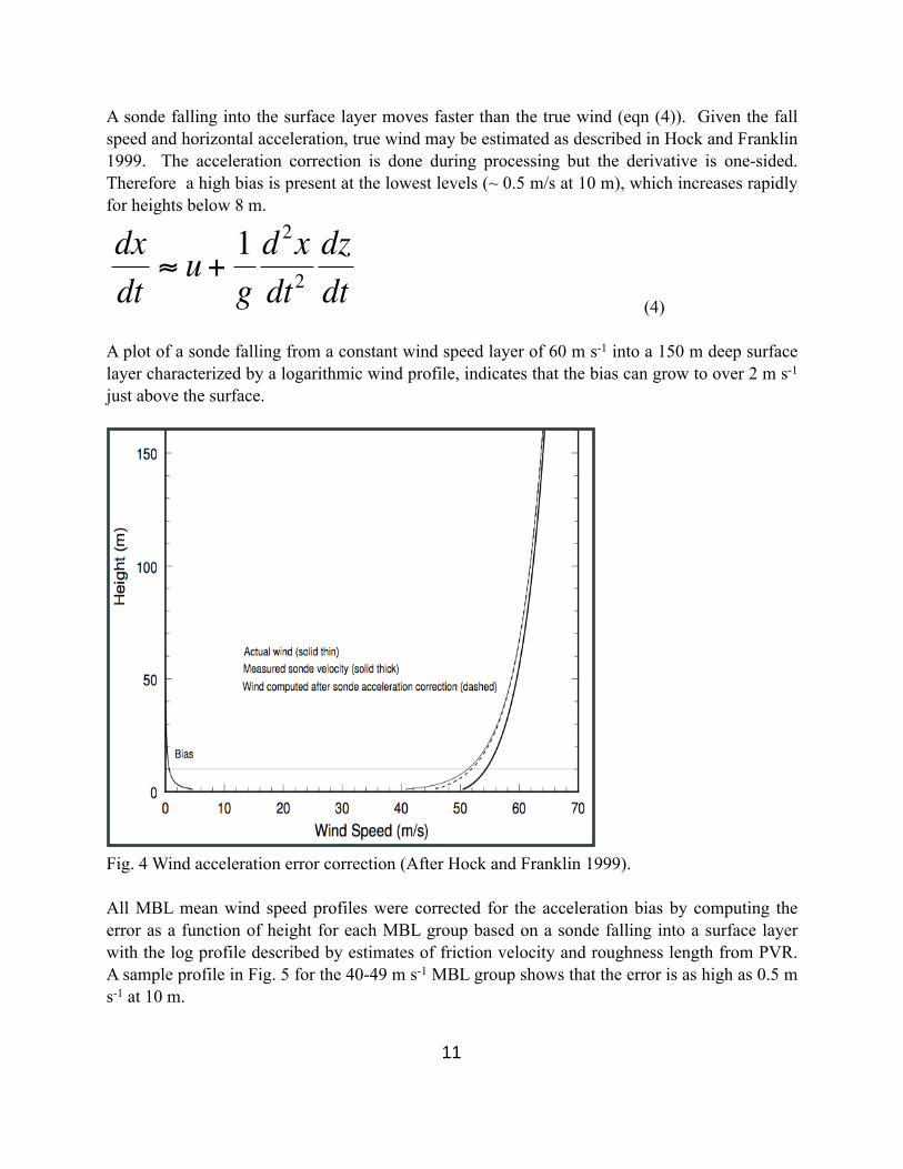
A sonde falling into the surface layer moves faster than the true wind (eqn (4)). Given the fall speed and horizontal acceleration, true wind may be estimated as described in Hock and Franklin 1999. The acceleration correction is done during processing but the derivative is one-sided. Therefore a high bias is present at the lowest levels (~ 0.5 m/s at 10 m), which increases rapidly for heights below 8 m.

€

dxdt

≈ u+1gd 2xdt2

dzdt

(4)

A plot of a sonde falling from a constant wind speed layer of 60 m s-1 into a 150 m deep surface layer characterized by a logarithmic wind profile, indicates that the bias can grow to over 2 m s-1 just above the surface.

Fig. 4 Wind acceleration error correction (After Hock and Franklin 1999).

All MBL mean wind speed profiles were corrected for the acceleration bias by computing the error as a function of height for each MBL group based on a sonde falling into a surface layer with the log profile described by estimates of friction velocity and roughness length from PVR. A sample profile in Fig. 5 for the 40-49 m s-1 MBL group shows that the error is as high as 0.5 m s-1 at 10 m.

11

Fig. 5 Plot of acceleration derivative error vs. Log10 of the height based on the 40-49 m s-1 MBL group in PVR.

Mean wind speed profiles were determined from the bin-average wind speeds for each MBL group. The profiles were plotted as Ln height vs. wind speed and a least squares linear regres-sion fit eqn (5) estimated the slope (ratio of the Von Karman constant (0.4) to the friction veloc-ity) and intercept (Zo, roughness length) for each MBL group.

Ln Z = (k/U*) U + Ln (Zo) (5)

12

€

Cd =.4

Ln Zo10

2

(6)

The drag coefficient was then computed from the roughness length. Since the number of sam-ples within the lowest two bins (8-12 m and 13-19m) was typically much less than that at 20-29 m, two estimates of the surface layer quantities were estimated. One estimate for the 8-150 m surface layer, and the second for the 20-150 m surface layer. Since sea surface temperatures are not available from the sondes, no attempt was made to compute a surface layer ψm value associ-ate with the departure of the wind profile from a neutral stability shape.

4. Results

4.1 Cd behavior with wind speed

Surface layer friction velocity, roughness length, and drag coefficient were computed based on linear least squares fits to the 20-160 m bin-average wind speeds. The mean surface layer wind profiles are shown in Fig. 6 for five MBL wind speed groups above 30 m s-1.

0 20 40 60 80

Wind Speed (m/s)

0.00001

0.0001

0.001

0.01

0.1

1

10

100

He

igh

t (m

)

0.00001

0.0001

0.001

0.01

0.1

1

10

100

0 20 40 60 80

Wind Speed (m/s)

0.0001

0.001

0.01

0.1

1

10

100

Heig

ht (m

)

0.00001

0.0001

0.001

0.01

0.1

1

10

100

60-69MBL40-49 MBL

13

Fig. 6 Mean wind profiles by MBL group. Symbols and bars represent bin mean and standard deviation. Least squares fit lines are extended to show the roughness length associated with the Y axis intercept.

Frequently the wind speed values in the lowest two bins diverge from a line through the remain-ing bins indicative of winds higher than the mean fit. This behavior is not indicative of wave sheltering but rather, near-surface winds stronger than that expected from a neutral stability log law. The lines shown in Fig. 6 were based on the 20-160 m layer, which is above the layer where the points diverge from the log profile. The roughness lengths determined from the inter-cepts of Fig. 6 were used to compute the drag coefficients (red squares) in Fig. 7.

30 35 40 45 50 55 60

U10 Neutral (m/s)

0

0.5

1

1.5

2

2.5

3

Cd

(*

10

00

)

10-160 m

95% Upper

95% Lower

20-160 m

95% Upper

95% Lower

452326 176

83

32

# Samples in 20-30 m bin

Fig. 7 Drag coefficient (squares) as a function of 10 m neutral stability wind speed. Upward and downward pointing triangles indicate the 95% confidence limits on the estimates. Numbers near each symbol indicate the number of wind speed samples in the 21-30 m bin.

Surface layer quantities are summarized in Table 1. Although the confidence intervals are similar with estimates based on the 10-160 m or the 20-160 m surface layers, the 20-160 m surface layer (without the 8-12 m and 13-20 m layers) have in general slightly better r2 values and less influ-ence from the departures of bin averages from the least squares fit line. We consider the 20-160 m layer to be more representative of the lowest levels that might be considered in mesoscale numerical prediction models such as HWRF. Drag coefficient behavior with wind speed shows a similar (to PVR, Fig. 8) initial increase with wind speed up to 10 m neutral stability wind speeds of about 42 m s-1, followed by a decrease as surface winds increase to ~ 62 m s-1. In comparison to PVR, the Cd values are all lower and the decrease is well defined. The large 95% confidence limits in Cd shown in PVR suggested that the Cd could either saturate or perhaps decrease,

14

whereas these results point to a well defined decrease, and now include the 70-79 m s-1 MBL group. This group contained insufficient profiles to conduct analysis in PVR. Too few profiles were available to conduct analysis for the 80-89 m s-1 MBL group. A recent paper in BAMS by Black et al., (2007) determined Cd (Fig. 9) using the SFMR measured surface wind speed and a friction velocity estimated by extrapolation of eddy correlation flux profile estimates between 70 and 400m. A total of 42 flux legs were flown in relatively clear regions outside of the main rainband convection in six regions of stepped-descent flight patterns in Hurricane Fabian and Isabel during the CBLAST field experiment. They claim that where Cd begins to decrease oc-curs at much lower wind speeds of 23 m s-1. The CBLAST Cd estimates have relatively large confidence limits such that it is difficult to attribute a transition wind speed; our Cd at 27 m s-1 falls within their error limits and they have no measurements for wind speeds above 29 m s-1.

20 30 40 50

U10 (m s )

0

1

2

3

4

CD

* 1

000

Hawkins and RubsamLarge and PondPalmen and Riehl

Miller Amorocho and DeVries

Shay

-1

c

10-100 m10-150 m20-100 m20-150 m

Fig. 8 Cd vs U10 from PVR

Fig. 9 Cd vs U10 from Black et al., 2007

15

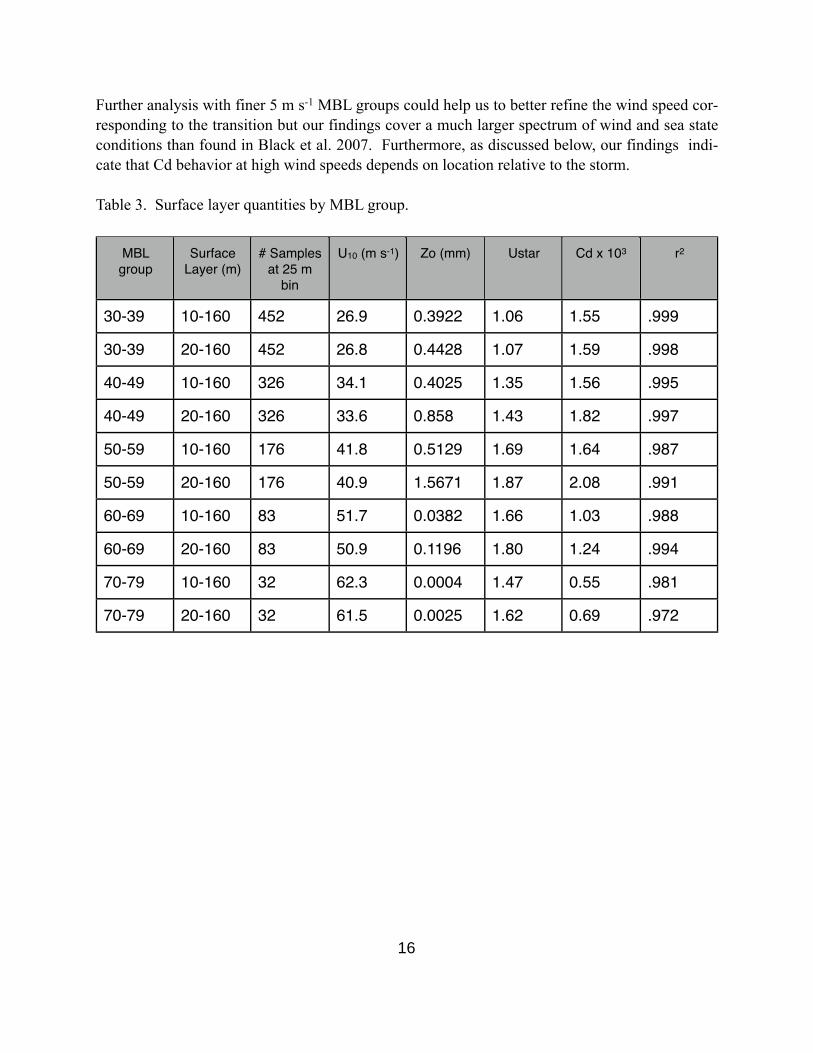
Further analysis with finer 5 m s-1 MBL groups could help us to better refine the wind speed cor-responding to the transition but our findings cover a much larger spectrum of wind and sea state conditions than found in Black et al. 2007. Furthermore, as discussed below, our findings indi-cate that Cd behavior at high wind speeds depends on location relative to the storm.

Table 3. Surface layer quantities by MBL group.

MBL group

Surface Layer (m)

# Samples at 25 m

bin

U10 (m s-1) Zo (mm) Ustar Cd x 103 r2

30-39 10-160 452 26.9 0.3922 1.06 1.55 .999

30-39 20-160 452 26.8 0.4428 1.07 1.59 .998

40-49 10-160 326 34.1 0.4025 1.35 1.56 .995

40-49 20-160 326 33.6 0.858 1.43 1.82 .997

50-59 10-160 176 41.8 0.5129 1.69 1.64 .987

50-59 20-160 176 40.9 1.5671 1.87 2.08 .991

60-69 10-160 83 51.7 0.0382 1.66 1.03 .988

60-69 20-160 83 50.9 0.1196 1.80 1.24 .994

70-79 10-160 32 62.3 0.0004 1.47 0.55 .981

70-79 20-160 32 61.5 0.0025 1.62 0.69 .972

16

4.2 Radial dependence of Cd behavior

Most sondes in the MBL wind speed groups > 50 m s-1 were launched according to a strategy to place them radially inward from the radius of maximum wind (to attempt to sample the surface maximum wind). The median of the radial distance of the drops in MBL groups > 50 m s-1 is near 30 km (Table 2) and we use this as a criterion for examining radial dependence of the mean wind profiles. It is advantageous to look at the mean profiles as a function of the actual radius rather than a scaled radial coordinate. A scaled coordinate would combine large and small storms together whereas, Kepert (2001, 2006) has shown that the curvature of the flow (in how it relates to inertial stability and relative angular momentum) is an important factor in the location and strength of boundary layer jets. A fixed radius of 30 km was selected to examine the de-pendence of the mean wind profile and surface layer characteristics at small and large radii.

30 35 40 45 50 55 60

U10 Neutral (m/s)

0

1

2

3

4

Cd

(*

10

00

)

10-160 m

95% upper

95% lower

20-160 m

95% upper

95% lower

74

58

89

41 21

# Samples in 20-30 m bin

30 35 40 45 50 55 60

U10 Neutral (m/s)

0

1

2

3

4

Cd

(*

10

00

)

10-160 m

95% upper

95% lower

20-160 m

95% upper

95% lower

378 268

87

42

11

# Samples in 20-30 m bin

Fig. 10 Cd vs U10 a) less than 30 km radial distance (top), b) > 30 km radius (bottom).

17

Cd values determined from mean wind profiles < 30 km from the storm center have fewer sam-ples (due to the majority of profiles in the 30-39 and 40-49 m s-1) with lower magnitudes and are relatively insensitive to changes in wind speed. Cd determined from profiles beyond 30 km show a more pronounced increase with wind speed up to about 40 m s-1 followed by a sharp de-crease at higher winds (although few samples are contained in the 70-79 MBL group estimates at surface winds of about 60 m s-1). While Rmax data are not yet available for all drops, it is likely that the profiles < 30 km are also radially inward from Rmax. The mean wind profile at small radii is associated with flow trajectories having greater curvature such that “new” waves are al-ways in a state of development and the sea state is characterized by the continuous breaking mechanism hypothesized by Donelan 2004. At larger radii with smaller trajectory curvature, the mean wind profile may be more influenced by interactions with waves that are in a more devel-oped state.

4.3 Cd behavior Azimuthal dependence

Results of the previous section indicate that region beyond 30 km radial distance is most likely to show an azimuthal signal in Cd behavior and this breakdown of the data have sufficient samples for further binning by storm relative azimuth. Indeed an important objective of this project is to investigate the azimuthal dependence of the drag coefficient. As depicted by this plot from Wright et al and Ed Walsh’s scanning radar altimeter wave data (Fig. 1) superimposed on an H*Wind analysis of Hurricane Bonnie of 1998, we can divide a storm into three regions (Black et al., 2007): 1) Rear sector (151-240 degrees relative to the storm motion vector) with 150-200 m long waves moving with the wind, 2) Right sector (21-150 degrees) with 200-300 m long waves moving outward by up to 45 degrees relative to the wind, and 3) Left front sector (241-020 degrees) where 300 m long waves travel outward at 60-90 degrees to the wind.

Figure 11. from Wright et al., 2001 showing wave and wind field for Hurricane Bonnie.

18

Analysis of the wind speed dependence of Cd in the right sector (Fig. 12) suggests that Cd is relatively invariant with wind speed, although an increase is suggested at winds > 45 m s-1.

30 35 40 45 50 55 60

U10 Neutral (m/s)

0

1

2

3

4

Cd

(*

10

00

)

10-160 m

95% upper

95% lower

20-160 m

95% upper

95% lower

169 123 56

23

# Samples in 20-30 m bin

Fig. 12 Cd vs U10 for radius > 30 km in the right sector of the storm (20-150 degrees) relative to the storm motion.

25 30 35 40 45 50 55 60

U10 Neutral (m/s)

0

1

2

3

4

Cd

(*

10

00

)

10-160 m

95% upper

95% lower

20-160 m

95% upper

95% lower

80

47

23

16

# Samples in 20-30 m bin

SR Az150-020

Fig. 13 Same as Fig. 12 but for Rear sector (151-240 degrees) relative to the storm motion.

19

30 35 40 45 50

U10 Neutral (m/s)

1

2

3

4

5

6C

d (

* 1

00

0)

10-160 m

95% upper

95% lower

20-160 m

95% upper

95% lower

129

98

24

16

# Samples in 20-30 m bin

SR Az150-020

Fig. 14 As in Fig 12 but for left front sector (241-020 degrees) relative to the storm motion.

In the rear sector (151-240 degrees) where the waves tend to move in the same direction as the wind, Cd is relatively constant and then decreases for winds above 34 m s-1 (Fig. 13). In the front left sector (241-020 degrees) the increase with wind speed behavior is very well defined with a maximum at winds of about 36 m s-1 and Cd values up to 4.7 x 10-3, followed by a rapid decrease as wind increase above 37 m s-1. In this sector the primary wave field moves crosswind as depicted in Fig. 11. For comparison, the data in Figs. 12-14 are superimposed in Fig. 15.

25 30 35 40 45 50 55

U10 Neutral (m/s)

1

2

3

4

5

6

Cd

(*

10

00

)

Left Front

Right

Rear

129

98

24

16# Samples in 20-30 m bin

SR Az150-020

80 4723

16

169

123 56

23

Fig. 15. As in Fig. 12 but summarizing results for the 20-160 m surface layer.

20

The superimposed Cd values for all storm relative azimuthal sectors in Fig. 15 show the rear sector slightly higher than the right for winds up to 35 m s-1, but the two sectors are similar for winds up to 42 m s-1. At higher winds Cd in the rear and left front both decrease considerably but the right sector shows a slight increase. These results suggest that Cd is most sensitive to wind speed in the left front sector, where scanning radar altimeter data suggest the waves have the longest wavelengths and tend to move outward 60-90 degrees crosswind. Data were insuffi-cient to establish Cd behavior for the 70-79 m s-1 MBL group. While the long wavelength waves resolved by the scanning radar altimeter are not directly relevant to the surface stress (associated with smaller high-frequency wind waves), the outward moving long period waves in the left front may modulate the wind wave field such that larger roughness elements are present. The sea state condition caused by smaller wind waves interacting with a fast swell moving outward crosswind, is apparently associated with larger surface roughness than found elsewhere in the storm. This condition is corroborated by examination of the Stepped Frequency Microwave Ra-diometer (SFMR) - GPS sonde difference pairs as a function of storm relative azimuth in a recent paper by Uhlhorn and Black (2003) and an updated version of their plot using 416 SFMR-GPS sonde pairs by Powell et al., 2007 (manuscript in preparation), reproduced in Fig. 16.

Fig. 16. Storm-relative azimuthal variation of bin-averaged SFMR-GPS sonde wind speed dif-ferences (m s-1). Curve with squares represents a harmonic fit to the bin averaged differences (x’s) and azimuth is measured clockwise from the direction of storm motion. From Powell et al., 2007.

This fit is used to correct the SFMR (which responds to emission from sea foam) for non-wind sources of roughness related to storm regions where wind seas are in the developing stage (more energy going into building the sea than being dissipated). In the right-rear the swell and wind are going in the same direction so the swell is growing and leaving less foam due to fewer breaking

21

waves (hence negative differences), while on the left front side the swells are generally propa-gating across the wind, leading to more breaking and more foam than wind seas alone (positive differences).

5. Discussion

Surface layer quantities were estimated from five mean wind profiles spanning MBL winds of 30-79 m s-1 and 10 m level neutral stability winds of 26-62 m s-1. All mean wind profiles but the 30-39 MBL exhibit kinks within 20 m of the surface such that some process must be allowing a stronger wind than expected from the log law, close to the surface. Arguments associated with wave sheltering would be associated with a kink in the wind profile in the opposite direction than that observed. Shallow unstable layers associated with relatively cool air over warm water, though observed, are unlikely as a primary mechanism since the instability would lead to greater vertical mixing, a condition that would inhibit profile kinks. A shallow stable layer with rela-tively warm air over a cooler sea surface could support a kink that would show increased shear, but such a kink would be in the opposite direction. The most likely explanation would be inter-facial properties that allow the flow in the lower two bins to be accelerated relative to flow over a more “normal” sea surface. This process would operate in the presence of shear and vertical velocity fluctuations that tend to well-mix the lower layers. Significant vertical motions are pre-sent at the lowest levels as shown in Fig. 17 for the 40-49 MBL group, and in the mean the verti-cal velocities are positive. The presence of generally positive vertical velocities is probably due to a combination of mesoscale forced upward motion associated with horizontal convergence, together with the buoyant plumes where relatively cool air overlies warm water.

1

10

7

5

3

2

100

70

50

30

20

Height(m)

-14 -10 -8 -6 -4 -2 0 2 4 6 8 10 12 14WComp(m/s)

Fig. 17 Vertical component of the wind speed as a function of height for the 40-49 MBL group.

A likely mechanism for the wind profile kinks would be the interfacial property of sea foam. PVR presented photographic evidence supporting enhanced sea foam coverage when winds are > 40 m s-1. They speculated that the surface properties of a sea foam emulsion could promote more

22

of a “slip” surface than a water surface. Andreas (2004) cited an obscure paper by Schmelzer and Schmelzer 2003 finding that bubble layers have lower surface tension and tensile strength than a water surface, hence a bubble layer would have difficulty supporting small-scale capillary waves that are thought to support stress at the sea surface. Andreas also speculated that spume and sea spray droplets support much of the stress near the ocean surface resulting in (assuming the total stress in the surface layer is constant with height) a decrease in stress supported by the air. He also suggested that sea spray and rain help to flatten the sea state and reduce roughness.

The foam mechanism may help to explain the relatively small Cd values within 30 km of the storm. In this location we hypothesize that the continuous breaking process described by Done-lan 2004 together with the resultant foam layer, is the predominant mechanism leading to re-duced Cd over a wide range of wind speeds. At radii beyond 30 km, the surface roughness is greatest and show the most sensitivity to wind in the left front quadrant where the swell propa-gates crosswind. There is a contradiction of processes in this quadrant since the crosswind swell promotes wave breaking and enhanced foam coverage but we also see the highest Cd values anywhere in the storm in this region. Our results suggest that in the left front sector, the interac-tion of the local wind waves with long-period, outward-propagating, crosswind swells contrib-utes to higher roughness and that despite indications of enhanced foam coverage, the scale of wave breaking is not sufficient to reduce the roughness until the winds exceed 36 m s-1.

6. Modeling Implications

The results from PVR and Donelan 2004 have motivated the modeling community to experiment with new parameterizations for the surface drag. Additional field results have corroborated the findings in PVR. Examples of Cd parameterizations include Chen et al., 2007 and Moon et al., 2004a,b. These approaches include “capping” Cd at some value when winds exceed hurricane force speeds. The 95% confidence limits on the PVR estimates of Cd were too large to deter-mine whether Cd saturated or decreased at extreme wind speeds. Now, with nearly 3 times the number of profiles, we have found that Cd indeed decreases in extreme winds. Recent inde-pendent oceanographic measurements in hurricanes support our finding (Shay and Jacob 2006, Jarosz et al., 2007). The behavior of Cd with wind speed is more complicated than a simple capping with wind speed but depends on location relative to the storm. We encourage modelers to experiment with parameterizations that allow Cd-wind behavior to vary by radial distance and storm relative azimuth. In idealized hurricane experiments with a couple wind-wave model , Moon et al., (2004b) found that the higher, longer, more fully developed waves in the right and front of the storm yielded older wave ages with higher values of Cd while lower shorter and younger waves to the rear and left yielded lower drag coefficients. In light of the inconsistencies with the findings reported here, further modeling investigations are warranted.

23

Acknowledgements

The PI benefited from discussions with Dr. Peter Vickery, who is conducting analysis with a sub-set of the GPS sonde data, and Dr. Peter Black, who shared some of his insights on wind wave interactions related to the CLAST experiments. Russell St. Fleur managed the loading and GPS sonde inventory associated with the database, as well as the JAVA interface. Nirva Morisseau-Leroy designed the Oracle database schema and query structure. This project was supported by a grant from the U. S. Weather Research Program’s Joint Hurricane Testbed.

24

References:

Andreas, E.L., 2004: Spray stress revisited. J. Phys. Ocean., 34, 1429-1439.

Black, P. G. and coauthors, 2007: Air-sea exchange in hurricanes: Synthesis of observations from the Coupled Boundary Layer Air-Sea Transfer experiment. Bull. Amer. Meteor. Soc., 88, 357-374.

Bender, M. A., I. Ginis, and Y. Kurihara, 1993: Numerical simulations of tropical cyclones- Ocean interaction with a high-resolution coupled model. J. Geophys. Res., 98, 23245-23263.

Chen S.S. and coauthors, 2007: The CBLAST-hurricane porogram and the next-generation fully coupled atmosphere-wave-ocean models for hurricane research and prediction., Bull. Amer. Me-teor. Soc., 88,311-317.

Donelan, M. A. B. K. Haus, N. Reul, W. Plant, M. Stiassnie, H. Graber, O. Brown, and E. Saltz-man, 2004: On the limiting aerodynamic roughness of the ocean in very strong winds. Geophys. Res. Lett, 31, L18306.

Emanuel, K.A., 1995: Sensitivity of tropical cyclones to surface exchange coefficients and a re-vised steady-state model incorporating eye dynamics. J. Atmos. Sci., 52, 3969-3976.

Franklin, J. L., 2000: Dropwindsonde processing on NOAA aircraft: EditSonde v5.04.

Hock, T.F. and J. L. Franklin, 1999: The NCAR GPS dropsonde . Bull. Amer. Meteor. Soc., 80, 407-420.

Jarosz, E., D. A. Mitchell, W. W. Wang, and W. J. Teague, 2007: Bottom-up determination of air-sea momentum exchange under a major tropical cyclone. Science, 315, 1707-1709.

Kepert, J.D., 2001: The dynamics of boundary layer jets within the tropical cyclone core. Part I: Linear theory. J. Atmos. Sci., 58, 2469-2484.

Kepert, J. D., 2006: Observed boundary layer wind structure and balance in the hurricane core. Part I: Hurricane Georges. J. Atmos. Sci., 63, 2169-2193.

Kepert, J. D., 2006: Observed boundary layer wind structure and balance in the hurricane core. Part II: Hurricane Mitch. J. Atmos. Sci., 63, 2194-2211.

Large, W.G., and S. Pond, 1981: Open ocean momentum flux measurements in moderate to strong winds. J. Phys. Oceanogr., 11, 324-336.

25

Moon, I. J., I. Ginis, and T. Hara, 2004: Effect of surface waves on Charnock coefficient under tropical cyclones., Geophys. Res. Lett, 31, L20302.

Moon, I. J., I. Ginis, and T. Hara, 2004:Effect of surface waves on air-sea momentum exchange. Part II Drag coefficient under tropical cyclones., J. Atmos. Sci., 2334-2348.

Panofsky, H. A. and J. A. Dutton, 1984: Atmospheric turbulence: Models and methods for engi-neering applications. John Wiley and Sons, N. Y., 397 pp. 397.

Pany, T., 2003: Tropospheric GPS slant delays at very low elevations. International workshop on GPS Meteorology. Tsukuba, Japan.

Powell, M. D., P. J. Vickery, and T. Reinhold, 2003: Reduced drag coefficient for high wind speeds in tropical cyclones. Nature, 422, 279-283.

Shay, L.K. and S. D. Jacob 2006: Relationship between oceanic energy fluxes and surface winds during tropical cyclone passage. Atmosphere-Ocean Interactions Volume II, Advances in Fluid mechanics, 115-142.

Uhlhorn, E. and P. G. Black, 2003: Verification of remotely sensed sea surface winds in hurri-canes. J. Atmos and Ocean Tech., 20, 99-116.

Vaisala, 2003: RD93_dropwindsonde.pdf, http://www.vaisala.com.

Wang, Y., and C.-C. Wu, 2004: Current understanding of tropical cyclone structure and intensity changes-A review. Meteor. Atmos. Phys., 87, DOI: 10.1007/s00703-003-0055-6.

Walsh, E. J., others, M. D. Powell, Black, and F. D Marks, Jr., 2002: Hurricane directional wave spectrum spatial variation at landfall. J. Physical Ocean., 32, 1667-1684.

Wright, C.W., others, M.D. Powell, Black, and Marks, 2001: Hurricane directional wave spectrum spatial variation in the open ocean. J. Phys. Ocean., 31, 2472-2488.

26