final report, frdc project 94/075: enhancement of yabby ... · final report, frdc project 94/075:...
TRANSCRIPT

Fisheries Western Australia
Fisheries Research DivisionWA Marine Research Laboratories
PO Box 20 NORTH BEACHWestern Australia 6020
Final Report, FRDC Project 94/075: Enhancement of yabby production from
Western Australian farm dams
FISHERIES RESEARCH REPORT NO. 112, 1998
Principal Investigator: Craig Lawrence
Project Staff: Noel Morrissy, Justin Bellanger
& Yuk Wing Cheng

Fisheries Research ReportTitles in the fisheries research series contain technical and scientific information that represents an important contribution to existing knowledge, but which may not be suitable for publication in national or international scientific journals.
Fisheries Research Reports may be cited as full publications. The correct citation appears with the abstract for each report.
Numbers 1-80 in this series were issued as Reports. Numbers 81-82 were issued as Fisheries Reports, and from number 83 the series has been issued under the current title.
EnquiriesFisheries Western Australia3rd floor SGIO Atrium168-170 St George’s TerracePERTH WA 6000Telephone (08) 9482 7333Facsimile (08) 9482 7389Website: http://www.wa.gov.au/westfish/res
Published byFisheries Western AustraliaPerth, Western AustraliaOctober 1998ISSN: 1035 - 4549ISBN: 0 7309 1984 6
Fisheries research in Western AustraliaThe Fisheries Research Division of Fisheries Western Australia is based at the Western Australian Marine Research Laboratories, P.O. Box 20, North Beach (Perth), Western Australia, 6020. The Marine Research Laboratories serve as the centre for fisheries research in the State of Western Australia.
Research programs conducted by the Fisheries Research Division and laboratories investigate basic fish biology, stock identity and levels, populations dynamics, environmental factors, and other factors related to commercial fisheries, recreational fisheries and aquaculture. The Fisheries Research Division also maintains the State data base of catch and effort fisheries statistics.
The primary function of the Fisheries Research Division is to provide scientific advice to government in the formulation of management policies for developing and sustaining Western Australian fisheries.

Contents PageList of Tables ........................................................................................................................iiiList of Figures .....................................................................................................................vii
Report Summary ................................................................................................................. 1
1.0 General introduction ....................................................................................................41.1 Background .............................................................................................................. 41.2 Need ......................................................................................................................... 51.3 Objectives ................................................................................................................ 5
2.0 General methods ...........................................................................................................62.1 Research station ...................................................................................................... 62.2 Industry farm dam recording system ....................................................................... 82.3 Genetics and Reproduction Laboratory ................................................................... 92.4 Experimental design and data analyses ................................................................. 10
3.0 Research station experiments .................................................................................... 11A) Variation between 25 research ponds .................................................................. 113.1 Physical, chemical and biological variation between 25 research ponds .............. 11
B) Density and feeding ............................................................................................. 193.2 .......................................................Effect of lowering density on the size of yabbies
193.3 Feeding lupins at the current industry standard rate vs non feeding ..................... 273.4 Effect of increased feed rates and alternative feeds on growth of yabbies ............ 29
3.4.1 Increased lupin feed rate vs CRD .............................................................. 293.4.2 Increased lupin feed rate vs CRD vs meat ................................................. 323.4.3 Increased CRD feed rates ........................................................................... 333.4.4 Low cost industry diets .............................................................................. 353.4.5 Variation in lupin control ........................................................................... 38
C) Mono-sex culture ................................................................................................ 403.5 Effect of single sex grow-out on size of male and female yabbies ........................ 40
D) Sediment oxidising agent .................................................................................... 493.6 The use of calcium nitrate to increase dissolved oxygen levels ............................ 49
E) Trap harvesting .................................................................................................... 553.7 Size and sex composition of yabbies in traps ........................................................ 55
4.0 Industry farm dam recording system .......................................................................56A) Baseline survey - yabby size, sex ratio and the farm dam environment ............ 564.1 The relationship between physical, chemical and biological parameters ............. 56
and yabby production in industry farm dams4.2 Size distribution and sex ratio of yabbies from industry harvested dams ............. 69
B) Application of feeding experiment results in farm dams ................................... 714.3 The effect of feeding upon the production of yabbies in farm dams ..................... 71
Fish. Res. Rep. Fish. West. Aust.1998, 112, 1-134
i

5.0 Genetics and reproduction laboratory ......................................................................77A) Habitats, morphology and speciation in the Australian wild yabby ................. 77
complex - significance for aquaculture5.1 Review of literature - taxonomy and distribution of the yabby Cherax ............... 77
albidus and related putative species and strains of freshwater crayfish5.2 Habitats of putative species and strains ................................................................. 905.3 The size of yabbies from different localities throughout Australia ..................... 105
B) The size at sexual maturity and sex ratio of selected yabby strains ................. 1095.4 Size at sexual maturity ......................................................................................... 1095.5 The sex ratio of strains ......................................................................................... 113
C) Hybridisation between yabby species and strains ............................................. 1155.6 Reproductive isolation and hybridisation ............................................................ 1155.7 The sex ratio of hybrids ....................................................................................... 1185.8 F1 fertility of hybrids ........................................................................................... 122
D) Growth rates of yabby strains and hybrids ....................................................... 1265.9 Growth rates of yabby strains and hybrids .......................................................... 126
6.0 General discussion ....................................................................................................129
7.0 Benefits .......................................................................................................................131
8.0 Further Development ...............................................................................................132
9.0 Appendices ................................................................................................................ 133Appendix 1: Intellectual property .............................................................................. 133Appendix 2: Staff ....................................................................................................... 133Appendix 3: Distribution list ..................................................................................... 133Appendix 4: Proximate composition of diets ............................................................ 134
Fish. Res. Rep. Fish. West. Aust.1998, 112, 1-134
ii

List of Tables PageTable 1 Nesting of Avondale research station experiments. .................................................7Table 2 Water chemistry parameters of Avondale research ponds at ...............................14
commencement and conclusion of experiments.Table 3 Average increase in weight per yabby at two different densities .........................21
and feeding regimes over 105 days.Table 4 Survival (mean±s.e., n = 6) of yabbies at two densities and feeding regimes. ......21Table 5 Density, biomass and feed rate for Research Station Experiment 5. .....................22Table 6 Final density and specific growth rate (SGR) of yabbies. .....................................23Table 7 Initial density, final density and survival of yabbies. .............................................23Table 8 Average increase in weight for fed and unfed yabbies at two densities ..............27
over 105 days.Table 9 Survival of yabbies at two densities and feeding regimes. ...................................28Table 10 Survival for the six treatments. .............................................................................30Table 11 Mean weight increase for three feeding regimes. .................................................30Table 12 Food conversion ratios (FCR) for three feeding regimes. ....................................31Table 13 Specific growth rates (SGR) for three feeding regimes. .......................................31Table 14 Mean weight increase for four feeding regimes. ...................................................32Table 15 Food conversion ratios (FCR) for four feeding regimes. ......................................32Table 16 Specific growth rates (SGR) for four feeding regimes. ........................................33Table 17 Survival for the four feeding treatments. ..............................................................33Table 18 Mean weight increase for four feeding regimes. ...................................................34Table 19 Food conversion ratios (FCR) for four feeding regimes. ......................................34Table 20 Specific growth rates (SGR) for four feeding regimes. ........................................34Table 21 Survival for the four feeding treatments. ..............................................................35Table 22 Mean weight increase for eight feeding regimes. .................................................36Table 23 Survival for eight feeding regimes. .......................................................................37Table 24 Food conversion ratios (FCR) for eight feeding regimes. ....................................37Table 25 Specific growth rates (SGR) for eight feeding regimes. ........................................37Table 26 SGR for the controls in five research station experiments. ...................................38Table 27 Table of the expected increase in weight of adult yabbies in each pond .............44
with different treatments and different sex by GLM.Table 28 Weight, growth and survival of male and female yabbies reared in ....................46
either mono-sex or mixed-sex populations over 175 days.Table 29 Table of the expected biomass used for social interaction by ..............................47
GLM, where C250 = CRD 2.5 g/m2/week; L250 = lupin 2.5 g/m2/week; and L500 = lupin 5 g/m2/week.
Table 30 Summary of results for mono-sex and mixed-sex populations of .......................47 C. albidus reared in ponds over 175 days (juveniles included).
Table 31 Mean bottom dissolved oxygen levels (mg/L) in calcium nitrate treated ............56 and untreated ponds for four feeding regimes: lupins at 2.5 g/m2/week (L2.5), lupins at 10 g/m2/week (L10), Crayfish Reference Diet at 10 g/m2/week (CRD10) and Meat at 10 g/m2/week (M10).
Fish. Res. Rep. Fish. West. Aust.1998, 112, 1-134
iii

List of Tables (continued) PageTable 32 Growth of yabbies fed on three different diets with and without ........................54
calcium nitrate.Table 33 Percentage of males and females collected from ponds by trapping ...................55
and draining (n = 410).Table 34 Summary statistics (minimum, maximum, median and mean) of the .................58
response variables for 21 farm dams.Table 35 Summary of water chemistry (mean, minimum and maximum) recorded .........59
during summer and winter from 21 WA farm dams currently harvested for yabbies (water quality criteria adapted from Langdon 1988; Train 1979; Hart 1974; Mills and Geddes 1980).
Table 36 Summary of chemical factors in summer with minimum, maximum, .................60 median and mean.
Table 37 Summary of chemical factors in winter with minimum, maximum, ................60 median and mean.
Table 38 Summary of physical factors with minimum, maximum, median .....................61 and mean.
Table 39 Matrix of correlations (r) between chemical parameters, yield, return ...............62 and density for summer and winter water samples from farm dams.
Table 40 Matrix of correlations (r) between physical parameters, yield, return .................63 and density from farm dams.
Table 41 Multiple linear regression results with “yield” as the response and ....................64 water chemistry in summer as predictor variables. Where R2 = 0.17 and residual standard error = 0.1752 (d.f. = 17).
Table 42 Multiple linear regression results with “return” as the response and ..................64 water chemistry in summer as predictor variables. Where R2 = 0.38 and residual standard error = 0.004343 (d.f. = 17).
Table 43 Multiple linear regression results with “return/cost” as the response ................64 and water chemistry in summer as predictor variables. Where R2 = 0.83 and residual standard error = 7.333 (d.f. = 17).
Table 44 Multiple linear regression results with “density” as the response and ................65 water chemistry in summer as predictor variables. Where R2 = 0 and residual standard error = 5.036 (d.f. = 20).
Table 45 Multiple linear regression results with “yield” as the response and ...................65 water chemistry in winter as predictor variables. Where R2 = 0.83 and residual standard error = 0.1177 (d.f. = 17).
Table 46 Multiple linear regression results with “return” as the response and ..................65 water chemistry in winter as predictor variables. Where R2 = 0.47 and residual standard error = 0.003615 (d.f. = 17).
Table 47 Multiple linear regression results with “return/cost” as the response and ...........65 water chemistry in winter as predictor variables. Where R2 = 0.83 and residual standard error = 7.733 (d.f. = 18).
Fish. Res. Rep. Fish. West. Aust.1998, 112, 1-134
iv

List of Tables (continued) PageTable 48 Multiple linear regression results with “density” as the response and ................65
water chemistry in winter as predictor variables. Where R2 = 0 and residual standard error = 4.429 (d.f. = 18).
Table 49 Multiple linear regression results with “yield” as the response and ...................66 physical factors as predictor variables. Where R2 = 0.85 and residual standard error = 0.083 (d.f. = 14).
Table 50 Multiple linear regression results with “return” as the response and ..................66 physical factors as predictor variables. Where R2 = 0.80 and residual standard error = 0.002088 (d.f. = 17).
Table 51 Multiple linear regression results with “return/cost” as the response and ...........66 physical factors as predictor variables. Where R2 = 0.46 and residual standard error = 8.00 (d.f. = 16).
Table 52 Multiple linear regression results with “density” as the response and ................66 physical factors as predictor variables. Where R2 = 0.997 and residual standard error = 0.2866 (d.f. = 18).
Table 53 Summaries of chemical factors and physical factors on the four responses ..........66Table 54 Size distribution according to weight grade and sex ratios of yabbies ................79
from 27 farm dams. Where n.s. = P > 0.5; * = P < 0.05; ** = P < 0.01; and *** = P < 0.001.
Table 55 Comparison of yield, return, management practices and economic return ..........73 for good and poor dams.
Table 56 Reclassification of C. destructor since Clark (1936). ...........................................78Table 57 Reclassification of C. albidus since Clark (1936). ................................................78Table 58 Summary of characters which distinguish C. albidus from C. destructor ...........79
(adapted from Sokol 1988).Table 59 Reclassification of C. esculus since Reik (1969). .................................................81Table 60 Reclassification of C. davisi since Clark (1941). ..................................................81Table 61 Reclassification of C. dispar since Reik (1951). ...................................................82Table 62 Reclassification of C. cuspidatus since Reik (1969). ............................................82Table 63 Reclassification of C. punctatus since Clark (1936). ............................................83Table 64 Reclassification of C. neopunctatus since Reik (1969). ........................................84Table 65 Reclassification of C. depressus since Reik (1951) ..............................................84Table 66 Reclassification of C. rotundus-setosus since Reik (1951). ..................................84Table 67 Reclassification of C. rotundus since Clark (1941). .............................................85Table 68 Collection sites - physical characteristics (* = max. depth of habitat; ..................93
** = the GPS data for this locality are known, but not presented in this report as it is the subject of a current investigation).
Table 69 Summary of water chemistry for collection sites. ................................................94Table 70 Comparison of relative proportions of ions (meq% l-1 ) of total ..........................95
cations and anions for collection sites.
Fish. Res. Rep. Fish. West. Aust.1998, 112, 1-134
v

List of Tables (continued) PageTable 71 Summary of combined summer and winter water chemistry ..............................96
(mean, minimum and maximum) recorded from a selection of WA farm dams currently harvested for yabbies (n = 52).
Table 72 Comparison of relative proportions of ions (meq%/L) of total ...........................96 cations and anions for a selection of WA farm dams currently harvested for yabbies (n = 52).
Table 73 Environmental parameters for Narrambeen, WA and ..........................................99 Merwyn Swamp, Vic.
Table 74 Size grade and average farm-gate price for yabbies from .................................106 collection localities.
Table 75 Localities, mean, minimum and maximum body weights, and .........................107 collection methods for yabbies.
Table 76 Maximum body weights of yabbies collected or reared in the .........................108 genetics laboratory.
Table 77 Minimum size and age of berried females from nine localities. ......................... 111Table 78 Sex ratio of juveniles from nine strains of yabbies. ............................................114Table 79 Reciprocal crosses from the nine populations of yabbies. ..................................117
Where: - = No mating; A = Berried but aborted eggs prior to hatching; D = Most or all juveniles died soon after release; and J = Juveniles produced.
Table 80 Sex ratio of yabby hybrids. .................................................................................120Table 81 Reproduction in hybrids from geographically separated populations ...............124
of yabbies. Where * = male-only F1 hybrids, refer section 5.7.Table 82 Specific growth rate (SGR), survival and final mean weights for each ...........127
of the nine yabby populations.Table 83 Specific growth rates of hybrids, survival and final weights. .............................127Table 84 Comparison of specific growth rates (SGRs) of hybrids with ...........................128
growth of both parent populations.
Fish. Res. Rep. Fish. West. Aust.1998, 112, 1-134
vi

List of Figures PageFigure 1 Location of logbook dams, Avondale research station and distribution of ...........8
yabby industry in Western Australia.Figure 2 Collection Localities. ..............................................................................................9Figure 3 Turbidity of research ponds at the commencement and conclusion of ................15
the experiment - the higher the Secchi disk depth, the lower the turbidity of the water.
Figure 4 Organic matter of pond sediment at the commencement and conclusion ............15 of the experiment.
Figure 5 Suspended organic matter (%) of pond water at the commencement and ...........16 conclusion of the experiment.
Figure 6 Mean yabby weight at commencement of experiment (Initial) and ....................16 variation in final yabby weights between pond blocks at conclusion of experiment (Block 1-6).
Figure 7 Weight gain of yabbies at different final densities after a 105 day ......................22 grow-out period.
Figure 8 The relationship of yabby survival (%) to initial stocking density. ......................24Figure 9 The relationship of final density at the conclusion of the ...................................24
experiment with initial stocking density.Figure10 The frequency distribution of six ponds with female yabbies .............................42
from different diet treatments (juveniles have been excluded), where F = females; C250 = CRD 2.5 g/m2/week; L250 = lupin 2.5 g/m2/week; and L500 = lupin 5 g/m2/week.
Figure 11 The frequency distribution of six ponds with male yabbies from ........................42 different diet treatments (juveniles have been excluded), where F = females; C250 = CRD 2.5 g/m2/week; L250 = lupin 2.5 g/m2/week; and L500 = lupin 5 g/m2/week.
Figure 12 The frequency distribution of six ponds with mixed-sex (1:1 ratio) ....................43 yabbies on different diet treatments (juveniles have been excluded), where A = mixed-sex; C250 = CRD 2.5 g/m2/week; L250 = lupin 2.5 g/m2/week; and L500 = lupin 5 g/m2/week.
Figure 13 The mean increase in weight of mixed-sex and mono-sex yabby .......................44 populations on three different diets, where M = male; F = female; A = mixed-sex; C250 = CRD 2.5 g/m2/week; L250 = lupin 2.5 g/m2/week; and L500 = lupin 5 g/m2/week.
Figure 14 Survival rate of mixed-sex and mono-sex yabbies fed three different ...............45 diets, where C250 = CRD 2.5 g/m2/week; L250 = lupin 2.5 g/m2/week; and L500 = lupin 5 g/m2/week.
Figure 15 Scatter plot of expected increased weight of yabbies with the number ...............46 of juveniles in each pond, where M = male; F = female; and A = mixed-sex.
Figure 16 Mean (± s.e.) surface and bottom water temperature and bottom ........................51 dissolved oxygen (DO) for calcium nitrate treated Ca(N0
3)
2 and untreated
ponds for four feeding regimes: lupins 2.5 g/m2/week (L2.5); lupins 10 g/m2/week (L10); crayfish reference diet 10 g/m2/week (CRD10); and meat 10 g/m2/week (M10).
Fish. Res. Rep. Fish. West. Aust.1998, 112, 1-134

List of Figures (continued) PageFigure 17: Mean (± s.e.) surface and bottom dissolved oxygen (DO) for calcium .................52
nitrate treated Ca(N03)
2 and untreated ponds for four feeding regimes: lupins
at 2.5 g/m2/week (L2.5); lupins at 10 g/m2/week (L10); crayfish reference diet at 10 g/m2/week (CRD10); and meat at 10 g/m2/week (M10).
Figure 18 Mean (± s.e.) water redox (mv) of calcium nitrate treated Ca(N03)
2 ...................52
and untreated ponds for four feeding regimes: lupins at 2.5 g/m2/week (L2.5); lupins at 10 g/m2/week (L10); crayfish reference diet at 10 g/m2/week (CRD10); and meat at 10 g/m2/week (M10).
Figure 19 Mean (± s.e.) pond sediment redox (mv) of calcium nitrate treated ....................53 Ca(N0
3)
2 and untreated ponds for four feeding regimes: lupins at
2.5 g/m2/week (L2.5); lupins at 10 g/m2/week (L10); crayfish reference diet at 10 g/m2/week (CRD10); and meat at 10 g/m2/week (M10).
Figure 20 Mean (± s.e.) depth of aerobic sediment (cm) of calcium nitrate treated ............53 Ca(N0
3)
2 and untreated ponds for four feeding regimes: lupins at
2.5 g/m2/week (L2.5); lupins at 10 g/m2/week (L10); crayfish reference diet at 10 g/m2/week (CRD10); and meat at 10 g/m2/week (M10).
Figure 21 Location of 21 logbook dams (D) and Avondale research station (A) ................56 in Western Australia.
Figure 22 Percentage composition of male and female yabbies by weight grade. ................70Figure 23 Relationship of average feed rate per week with yield of yabbies/week. .............73Figure 24 Comparative size distribution of good and poor producing dams. .......................74Figure 25 Yabby yield in dams H1 (good producing) and H2 (poor producing). ................74
Lupins were replaced with CRD (0.5 g/m2/week) in H2 January 1997.Figure 26 Yabby yield in dam E2 (good producing) and E3 (poor producing). ..................75
Lupins were replaced with CRD (2.86 g/m2/week) in E3 in March-June 1997.
Figure 27 Yabby yield in dam F1 (poor producing) and F3 (good producing). ...................75 Lupins and oats were supplemented with CRD (2.0 g/m2/week) in F3 in January 1997.
Figure 28 Distribution of yabbies according to Reik (1969). ................................................86Figure 29 Distribution of yabbies according to Sokol (1988). ..............................................87Figure 30 Distribution of yabbies according to Austin (1988). .............................................87Figure 31 Collection localities. Where D = Dalhousie Springs; A = Algebuckina; ............92
C = Clayton; MS = Merwyn Swamp; N = Nurrabiel; B = Barmah Forest; SM = Murrumbidgee River; PR = Nundle, Peel River; BC = Barrack Creek; LH = Lake Hiawatha; OC = Oxley Creek; K = K***; and WA = Narembeen.
Figure 32 Weight (g)-length (OCL mm) relationship for WA yabbies. ...............................110Figure 33 Minimum size (OCL) of berried females from nine localities. ........................... 111
Fish. Res. Rep. Fish. West. Aust.1998, 112, 1-134
viii

Fish. Res. Rep. Fish. West. Aust. 1998, 112, 1-134
1
Report Summary
Report title: 94/075 Enhancement of yabby production from Western Australian farm dams
Principal Investigator: Craig Lawrence
Address: Western Australian Marine Research Laboratories Fisheries WA PO Box 20 NORTH BEACH WA 6020
Objectives
To increase harvests from WA farm dams by providing farmers with: 1. Population control method(s) which increase the proportion of yabbies of marketable
weights; 2. Quantified methods for feeding and improving farm dam environmental factors limiting
yabby production and causing variation in dam productivity; 3. Establishing methods for managing yabby stocks and farm dam productivity to increase
harvest per dam; 4. A manual of methods for stocking and managing farm dams to increase harvest per dam. Non-technical Summary
Farmers receive higher prices per kilo for large yabbies. Yabby farmers have reported that the majority of yabbies trapped from farm dams are below market size (< 30 g) and therefore of no economic value. In addition, farmers also report that while dams produce large yabbies when first harvested, after a number of years the proportion of large animals gradually decreases. To identify why yabbies in farm dams stunted and how farmers could increase the size of small yabbies the project had three main experimental areas. Research station experiments: A field research station consisting of 25 ponds was constructed for running replicated, randomised and reproducible experiments, with controls, in an environment that simulated farm dams. In addition, these ponds were large enough to provide an adequate sample number of yabbies at realistic industry stocking densities. At this facility researchers investigated feed types, feed rates, stocking densities, mono-sex culture, chemical additives and trapping. Industry farm dam recording system: Researchers worked with farmers to establish a recording system covering the 750,000 km2 yabby harvesting region in WA. Farmers maintained logbooks of yabby harvests, feeding regime and management practices. Researchers recorded physical, biological and chemical parameters from each dam. Logbook information provided industry data on factors affecting yabby yields and results of technology transfer from the research station. Genetics and Reproduction Laboratory: Yabbies were collected from around Australia and transported alive back to a secure quarantine laboratory in Perth. The yabby strains were compared under identical controlled conditions to evaluate the relative aquaculture potential of both different “varieties” and hybrids, in particular size, growth, size/age at sexual maturity and sex ratio.

Fish. Res. Rep. Fish. West. Aust. 1998, 112, 1-134
2
Results
This project has shown that population control methods to increase the proportion of marketable yabbies are required, as: • The growth rates of yabbies are inhibited at higher densities • Lower stocking densities result in larger yabbies • Density has over twice the influence upon yabby growth than current industry feeding
regimes using lupins • Trapping of farm dams selectively removes the largest male yabbies, resulting in a higher,
proportion of the remaining population consisting of breeding females and small males • The trapping induced yabby population structure results in a high density of juvenile
yabbies with reduced growth A low cost method of controlling population density is mono-sex culture, the advantages of mono-sex culture are: • Male yabbies grow 68% faster than female yabbies • In mono-sex culture male yabbies grow 17% faster than males in mixed-sex populations.
Female yabbies in mono-sex culture grow 31% faster than in mixed-sex culture • The increased size of yabbies harvested provides a 70% increase in gross return to the
farmer • To enable the practical application of mono-sex culture, and consequently control density,
a method of producing yabbies of only one sex has been discovered
Given that mono-sex culture provides larger yabbies, a strain or hybrid that did not breed would save labour costs required for hand sexing. Investigation of yabby “varieties” around Australia has shown some potential for both strain selection and population control. • There is considerable variation in the aquaculture potential of yabbies from different
regions of Australia. In particular, a number of strains fail to grow to 30 g, the minimum market size
• The introduced WA “albidus strain” appears to be as good as, or superior to, most of the other Australian strains evaluated in this study
• A number of hybrids produced in this study have, at this stage, shown preliminary evidence of hybrid sterility and/or heterosis
• All male hybrids can be produced by mating female K sp. yabbies with male “albidus” yabbies
Feeding farm dams can improve yabby harvests. • The current industry supplementary feeding regime based upon lupins gives an improved
growth rate (32%) • Growth rates can be increased an additional 85% using improved diets • Calcium nitrate can increase dissolved oxygen levels in ponds and oxidise anaerobic
sediments. This technology may permit higher feeding levels, in non-aerated ponds The most important farm dam environmental factors limiting yabby production are: • Feed (low feeding rates, height on catchment), aeration (low wind exposure, high banks)
and production area (small size, high density) • Water chemistry parameters were recorded at levels that may limit yabby production and a
relationship between some of these factors and yield has been demonstrated • Compared with chemical variables, physical factors were more important in limiting yabby
production from WA farm dams
Methods established for managing yabby stocks and farm dam productivity to increase harvest per dam, including different feed types, rates, hybrids, mono-sex and stocking

Fish. Res. Rep. Fish. West. Aust. 1998, 112, 1-134
3
densities are presented in FRDC Report 94/075 and are being prepared for inclusion in the Yabby Industry Code of Practice and a range of extension material. General Conclusions
This study has shown that it is possible to convert yabbies below market size (< 30) to high value animals by improving feeding and management practices. The application of these results will produce larger yabbies and directly result in increased returns to farmers. In addition the increase in market-sized yabbies from farm dams will provide a higher catch rate per unit of trapping effort. Consequently, the harvesting of yabbies from more isolated dams will become economically viable. The current FRDC project (FRDC 97/319) builds upon these results and further investigates feeding, nutrition, aeration, husbandry, indicators of productive dams and polyculture. This information will result in a comprehensive manual on farm dam yabby production. Additional research into the potential of hybrids is the subject of a funding application. Keywords: Cherax albidus, crayfish culture, pond culture, aquaculture techniques, feeding, stocking density, reproduction, hybrid culture.

Fish. Res. Rep. Fish. West. Aust. 1998, 112, 1-134
4
1.0 General introduction
1.1 Background In the large inland south-west agricultural region of Western Australia farmers have considerable incentive to diversify due to decreased returns from traditional cropping and sheep raising. The main new avenue has been harvesting yabbies (Cherax albidus) which have long been introduced to stock dams there. The harvesting of yabbies from dams requires little capital input, since existing water bodies are used. Consequently, this simple form of aquaculture is readily available to farmers and has been increasingly taken up by them, profitably. This success compares to suggested alternative; more intensive methods for yabby aquaculture that require significant capital expenditure for purpose-built ponds or tank systems and water supply and have not been as successful as farm dam harvesting in Australia. The WA yabby aquaculture industry has shown rapid growth, from 1.7 tonnes in 1987 to 286 tonnes in 1994 ($2.8 million), a significant proportion of which was exported alive. Successful export of the premium live product to European and Asian restaurant markets has been led by several WA processing entrepreneurs, committed to high post-harvest product quality.
Using conservative values for annual harvest per dam and the number of exploitable dams (approximately 100,000 at present), the yabby industry has the potential to reach 5,000 tonnes per annum, worth $50 million in export. As well as industry growth via exploitation of an increasing number of dams, examples of expansion provided by developed aquaculture industries elsewhere indicate that growth should also occur through distinctive jumps in efficiency, i.e. increased harvest per unit area of water, provided by appropriate research. The increased efficiency in production may be of the order of five times the start-up level of an embryonic industry.
We and our industry collaborators recognise two main aspects of the yabby production system which have been limiting efficiency, these are:
i) the lack of industry methods for managing yabby stocks, particularly the inherent trend of the species towards stunting of stocks; and
ii) means for overcoming the aquacultural limitations of the farm dam environment, particularly in regards to feeding and aeration.
Although general biological information on yabbies is available and other, more intensive, culture systems have been suggested by researchers elsewhere in Australia (e.g. Mills and McCloud 1983), little of this work is directly applicable to further improvement of the harvest rate per dam for the WA yabby culture system, which is based upon undrainable farm dams in the inland, south-west region. The WA yabby region is characterised by very marked winter rainfall-summer drought pattern, unique water quality and soil (clay) types, and the fact that yabbies are a particular species introduced from the diverse eastern states "yabby complex" of species and sub-species.

Fish. Res. Rep. Fish. West. Aust. 1998, 112, 1-134
5
1.2 Need Farmers, processors and exporters have widely perceived two needs for research.
1. To provide a stock management technique for preventing stunting of yabbies in farm dams.
Current catches generally show a low proportion of yabbies of marketable weight. High density due to uncontrolled reproduction in farm dams, and the high fecundity of yabbies, is thought to result in growth stunting of most of the large biomass of yabbies and poor survival through to larger body weights. The price per kilo of marketed yabbies is strongly related to the weight grade in the 20 to > 80 g range.
2. To identify and provide means for improving dam environmental factors limiting production.
Farmers and harvesters have observed a significant variation in yabby harvests between dams. This variation strongly suggests that production can be increased in many dams. The assumed benefit of the current laissez faire method of feeding readily available lupins to yabbies needs to be quantified experimentally for farmers. As well, the nutritional adequacy of the lupins has been questioned by a leading farmer, noting declining harvests, and so needs to be examined. The interaction between feeding and natural eutrophication of dams, due to valley location and catchment type, needs to be taken into account by farmers and is poorly understood at the moment. Strong relationships between crayfish production and water calcium level have been documented in previous work (Morrissy 1980). Many yabby dams are thought to be deficient in calcium which is needed for crayfish shell formation and this condition may be exacerbated by crayfish removal.
1.3 Objectives To increase harvests from WA farm dams by providing farmers with: • Population control method(s) which increase the proportion of yabbies of marketable
weights • Quantified methods for reducing dam environmental factors limiting yabby production and
causing variation in dam productivity • A manual of methods for stocking and managing farm dams to increase harvest per dam

Fish. Res. Rep. Fish. West. Aust. 1998, 112, 1-134
6
2.0 General methods
2.1 Research station Experiments were performed at the Avondale research station (feed, density, mono-sex, etc.) and results applied to industry farm dams, using the highly successful R&D model provided by Agricultural plot experiments and farmer demonstration trials. Previous studies into yabby production, and in particular grow-out trials, encountered difficulties in obtaining accurate data due to one or more of the following factors. 1. Experiments on crayfish in glass aquaria and fibreglass tanks fail to adequately reflect
complex and dynamic pond ecosystems. The aquaculture industry in general has repeatedly experienced difficulties when attempting to apply the results of small scale laboratory experiments to commercial grow-out farming systems.
2. Farmers will not permit the draining of dams, particularly during the summer growing season, to catch all the yabbies so that researchers may accurately quantify yabby population structure and biomass; which is vital to precisely assess the results of treatments.
3. Experience has shown a need to avoid the time consuming and analytically complex sampling using baited traps for the capture mark release recapture (CMRR) method for indirectly assessing yabby dam populations.
4. Industry has reported significant levels of variation between farm dams.
5. Experimental design and results in field experiments have been compromised by the lack of replication of treatments and a multitude of varying factors which cannot be controlled.
To address these concerns, particularly the problems of environmental variation between dams and adequate replication of treatments, a field facility of experimental dams was constructed. These dams were scaled replicas of the common clay farm dam used for yabby production and could be drained to obtain data on total yabby numbers by weight grade category. The Avondale research station near Beverley demonstrated the following favourable characteristics: • Clay representative of the Wheatbelt yabby farming region. • Known history of cropping and chemical use, similar to yabby industry farming properties
in the region. • Resident caretaker staff. • Adequate rainfall and catchment. • Sufficient room for building ponds. • Centrally located for ease of access by industry. • Security of tenure. • Support and co-operation of farm management and Agriculture WA employees.
The site was surveyed and pegged. The facility was built in the 12 week period between 22 June and 22 September 1994.
The farm dam research facility constructed at the Avondale research station was supplied by a 10,000 m3 water supply dam. The dam filled by run-off from a 4 ha roaded catchment leading to a piped inlet, in addition to the 82 ha of catchment from land used for pasture. This source of water is similar to the water source for WA. Wheatbelt farm dams, i.e. catchment run-off.

Fish. Res. Rep. Fish. West. Aust. 1998, 112, 1-134
7
From the dam a 750 m pipeline supplied water to each of the 25 experimental ponds and thus provided a homogeneous water supply for all experimental ponds. Ball floats maintained water levels in each pond at the same level.
Each experimental pond was a scaled down version of a farm dam: 100 m2 in water surface area and 1.5 m deep, with a drain, standpipe and concrete sump to allow for complete emptying to harvest all yabbies. Each pond profile was built to represent a miniature farm dam and was constructed from clay with a 3:1 batter (bank drop of 1 m in every 3 m) and similar ratios between wall and water surface area to normal full-sized dams. Stainless steel mesh screens were placed on the sump prior to removal of the standpipes to prevent yabbies from being drawn down the drain. The drains consisted of 690 m of pipe laid 3 m below ground level leading to the sump. The system was designed so that water drained from ponds could be salvaged from the sump and returned to the large storage dam for reuse at a later date. The ponds were protected from run-off by a 300 m contour bank up hill of the ponds, which directed excess water away from the ponds and into the sump. Each pond was netted individually to prevent bird predation and each was also fenced to prevent movement of yabbies from one pond to the other, in particular exchange between single sex populations.
Prior to stocking the first experiment in spring 1994, pond sediments were conditioned using sheep manure to obtain similar levels of organic matter (4%) to that found in existing farm dams. Initial water chemistry, sediment organic matter, suspended organic matter, invertebrate composition and turbidity were recorded (section 3.1).
With 25 ponds available for replication, and as the inherent variation between ponds was known after the first experiment, it was possible to examine a number of treatments concurrently by nesting within each experiment (Table 1). Dams were randomly assigned to treatments, which were nested within blocks of ponds. Detailed methods for each research station experiment are provided in sections 3.1 to 3.7. All experiments at the research station ran for a minimum of 100 days and were timed to correspond with the yabby growing season from September to May. At the conclusion of each experiment ponds were trapped and drain-harvested over a five day period (five ponds per day) and all animals were collected, sexed, weighed and measured. Table 1 Nesting of Avondale research station experiments.
Experiment Treatments Investigated
Experiment 1 Physical, chemical and biological variation between research ponds. Growth of yabbies at high vs low stocking density. Growth of yabbies fed lupins vs no feeding.
Experiment 2 Growth of yabbies with increased feeding rates of lupins vs feeding CRD. Comparing the growth of mono-sex with mixed-sex yabby stocking.
Experiment 3 Growth of yabbies with increased lupin feeding vs increased CRD vs meat. Influence of calcium nitrate on dissolved oxygen, water quality, sediments and growth of yabbies.
Experiment 4 Growth of yabbies at increased CRD feed rates.
Experiment 5 Comparison of low cost industry diets (oats, barley, wheat, lupins, fertiliser, CRD and meat meal). The effect of increased stocking density on mean harvest weight of yabbies.

Fish. Res. Rep. Fish. West. Aust. 1998, 112, 1-134
8
2.2 Industry farm dam recording system Farmers reported a large variation in yabby production between individual farm dams in the Western Australian Wheatbelt. In order to identify the most productive dams and farming techniques, the variation between dams, current yields and management practices need to be recorded quantitatively. To record data, a log book system was established.
Individual volunteer farmers filled out log books based upon their anecdotal levels of yabby production and characteristics of farm dams. Each of these farmers was visited during November-December 1995. Researchers explained logbooks to farmers and sampled dams for water and sediment. Dams were photographed, measured and categorised according to aspect, clay type, water colour, turbidity, dissolved oxygen and temperature. This initial survey established the baseline data for a logbook system monitoring yields and management practices covering 750,000 km2, ranging from Northampton in the north, Esperance in the south and east to Mukinbudin (Figure 1). For each of the 30 dams in the study, farmers or harvesters maintained a logbook to provide accurate records of harvests, feeding and management practices for each dam. Dams were selected to reflect the diverse range of locations and environments which are used to farm yabbies in Western Australia (i.e. northern vs southern, coastal vs inland, high on catchment vs low on catchment, new vs old, etc.).
H1 H2H3
D1 D2D3
A1 A2A3
C1 C2
B1 B2
F1 F2F3
E1 E2E3
G1 G2
PERTH
ALBANY
BEVERLEY
NARROGIN
ESPERANCE
MUKINBUDIN
NORTHAMPTON
Avondale Research Station
Figure 1 Location of logbook dams, Avondale research station and distribution of yabby industry in Western Australia.
Logbook dams were trawled using a seine net by research staff between 18 June 1996 and 27 August 1996 to obtain size distributions of yabbies. Although trawling may result in physical damage to the yabbies it provides a more accurate assessment of the population, as unlike sampling by baited traps, it is not size or sex selective.
Fish. Res. Rep. Fish. West. Aust. 1998, 112, 1-134
9
Upon the receipt of yabby yields for the 1995-96 harvesting season, correlations between farm dam production and environmental parameters were obtained. Based upon information from the logbooks giving baseline data, improved feeding and management techniques developed at the Avondale research station were implemented in the logbook dams and records of their effect upon yabby production were obtained in 1996/97 harvesting season.
2.3 Genetics and Reproduction Laboratory This component of the project addresses the first objective: developing a population control method. The aim was to control the reproduction of yabbies in farm dams by either: a) identifying an Australian strain with lower female fecundity or a skewed sex ratio; or b) producing a hybrid which was sterile or had a skewed sex ratio.
In addition, researchers also investigated the question of whether the WA strain is superior or inferior to stocks in the eastern states.
There is a large number of closely related yabby species, subspecies and strains in the wild, adapted to a very wide range of environmental conditions (desert to mountain) (Sokol 1988; Austin 1996). The type localities of the so-called destructor complex have been well documented (Clark 1936, 1941; Reik, 1951, 1956, 1969; Sokol 1988). Within the broad distribution of yabbies, those strains throughout Australia which offer the most potential for contributing to diverse stock were identified. Yabby populations were selected according to the following factors: • Allopatric populations which are likely to have been segregated for sufficient time to have
acquired reproductive incompatibility with each other; • Populations representative of the broad range of ecotypes of yabbies adapted to diverse
environments; and • Genetically “pure” populations, as opposed to populations which are the result of recent
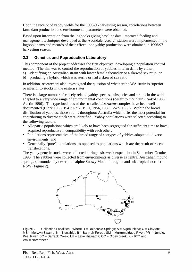
translocations. The yabby genetic stocks were collected during a six-week expedition in September-October 1995. The yabbies were collected from environments as diverse as central Australian mound springs surrounded by desert, the alpine Snowy Mountain region and sub-tropical northern NSW (Figure 2).
#
#
#
##
# #
# #
#
DA
C MSN
B SM
PRBC LH
OC
KWA
Figure 2 Collection Localities. Where D = Dalhousie Springs; A = Algebuckina; C = Clayton; MS = Merwyn Swamp; N = Nurrabiel; B = Barmah Forest; SM = Murrumbidgee River; PR = Nundle, Peel River; BC = Barrack Creek; LH = Lake Hiawatha; OC = Oxley creek; K = K*** and WA = Narembeen.

Fish. Res. Rep. Fish. West. Aust. 1998, 112, 1-134
10
The expedition obtained 12 different populations of yabbies representing strains of Cherax destructor and Cherax albidus, a number of closely related species, such as C. dispar, C. rotundus, C. cuspidatus, and one as yet undescribed yabby thought to be a new species of Cherax. (Note: since the collecting expedition Austin 1996 has published a revised taxonomy of the ‘yabby complex’, see section 5.1).
The yabbies were transported alive back to a newly established genetics laboratory in Perth where they formed the basis of a gene pool for investigating the genetics and reproduction of Cherax spp. The University of Western Australia provided land and a building in Perth and staff from Fisheries WA installed 104 individual aquaria each 120 L capacity and five sets, each of 10 battery tanks, for breeding trials. The facility was prepared to satisfy strict state quarantine protocols. Each aquarium had a recirculating filtration system, and was either heated to allow for winter breeding or maintained at ambient temperature. Water quality was maintained by biofilters. Yabbies were fed daily to satiation on the crayfish reference diet and earthworms. The yabby strains were compared under identical controlled conditions to evaluate the relative aquaculture potential, in particular size, growth, size/age at sexual maturity, fecundity, sex ratio and morphology of different populations of Cherax spp. and hybrids.
Breeding populations of the strains were established and trials of the populations collected commenced in December 1995.
2.4 Experimental design and data analyses Experiments at both the Avondale research station and the Genetics and Reproduction Laboratory were designed in consultation with statisticians from the WA Marine Research Laboratories, Fisheries WA Research Division. This ensured that sound experimental principles (controls, replication, reproducibility and randomisation) were adhered to in this study. Individual experimental designs are presented in greater detail in sections 3.1 to 5.9.
Growth rates are presented as specific growth rate (SGR), in accordance with the standard reporting approach for describing freshwater crayfish growth proposed by Evans and Jussila (1997). Data at the conclusion of experiments have been analysed with the assistance of statisticians from the WA Marine Research Laboratories using S-Plus, SAS, Excel and Arc Info. References
Austin, C.M. 1996. Systematics of the freshwater crayfish genus Cherax Erichson (Decapoda: Parastacidae) in northern and eastern Australia: electrophoretic and morphological variation. Aust. J. Zool., 44: 259-296.
Clark, E. 1936. The freshwater and land crayfishes of Australia. Mem. Nat. Mus. Vict., 10: 5-58.
Clark, E. 1941. New species of Australian freshwater and land crayfishes (Family Parastacidae) Mem. Nat. Mus. Vict., 12: 31-41.
Evans, L and Jussila, J. 1987. Freshwater crayfish growth under culture conditions: Proposition for a standard reporting approach. J. World Aqua. Soc., 28(1): 11-19.
Mills, B.J. and McCloud, P.I. 1983. Effects of stocking and feeding rates on experimental pond production of the crayfish Cherax destructor Clark (Decapoda: Parastacidae). Aquaculture, 43: 51-72.

Fish. Res. Rep. Fish. West. Aust. 1998, 112, 1-134
11
Morrissy, N.M. 1980. Production of marron in Western Australian farm dams. Fish. Res. Bull., 24, 79p.
Raeburn, P. 1995. The last harvest. Simon & Schuster, New York, 269p.
Reik, E.F. 1951. The freshwater crayfish (Family Parastacidae) of Queensland. Rec. Aus. Mus., 22: 368-388.
Reik, E.F. 1956. Additions to the Australian freshwater crayfish. Rec. Aus. Mus., 24: 1-7. Reik, E.F. 1969. The Australian freshwater crayfish (Crustacea: Decapoda: Parastacidae),
with definitions of new species. Aust. J. Zool., 17: 855-918. Sokol, A. 1988. Morphological variation in relation to the taxonomy of the destructor group
of the genus Cherax. Invertebr. Taxon., 2: 55-79.
3.0 Research station experiments
A) Variation between 25 research ponds 3.1 Physical, chemical and biological variation between 25 research ponds Introduction
Agricultural plot experiments on field research stations provide a bridge between glass house experiments and industry paddocks (Fisher 1958, 1960). Similarly, aquaculture pond experiments provide both a bridge between aquarium studies and commercial ponds, and a more realistic estimate of production than laboratory aquarium or tank studies which tend to underestimate yields (Shell 1983).
Research station experiments include most of the advantages of true ecological studies where the population of animals is influenced by many uncontrolled natural factors, as is experienced in commercial ponds. This is in contrast to classical experimentation where usually a single factor is assessed under highly controlled conditions in the laboratory.
However, aquarium experiments on crayfish in tanks do not provide the clay sediment substrate, or algal and clay turbidity present in commercial production systems. Long-term growth performance and nutritional health of crayfish are usually so poor in clean tanks that experimental comparisons are compromised (Morrissy 1984). Furthermore laboratory tank experimentation is impracticable at industry densities of 1-5 yabbies/m2. Since density and growth of freshwater crayfish are highly inversely related (Morrissy 1992), tank experiments at high densities are very unrealistic and give poor growth and survival. Industry farm dams each contain many thousands of yabbies and the labour required to accurately assess growth and population numbers is unnecessarily high. In the yabby farming industry in Western Australia, “commercial ponds” are argillotrophic, clay-based, paddock catchment dams filled by rainfall run-off to provide drinking water for sheep. There are large, mostly uncontrolled variations in many physical, biological and yabby management practices among widely dispersed dams (Morrissy 1974; Cheng et al. in prep). Also stocks of yabbies in these dams cannot be assessed easily or accurately because the dams are not drainable. To carry out yabby grow-out experiments, a research facility consisting of 25 ponds with a homogeneous water supply from a header dam was built near Beverley Western Australia (latitude 32°7’ south, longitude 116°55’ east). This facility was capable of running replicated,

Fish. Res. Rep. Fish. West. Aust. 1998, 112, 1-134
12
randomised and reproducible experiments, with controls, in an environment that simulated farm dams. In addition, these ponds, each 100 m2 in surface area, also provide an adequate sample number of yabbies at realistic industry stocking densities (1-5 yabbies/m2).
Large variability between ponds in aquaculture experiments often leads to imprecise estimates of treatment effects. Previous workers in classical agricultural field experiments, such as at Rothamsted (Fisher 1958, 1960) and aquaculture pond trials at Auburn (Shell 1983), emphasised that in order for results from grow-out experiments to be analysed and evaluated, it is important to first: i) demonstrate that the experimental units are homogeneous; or ii) quantify any variation between plots, ponds or blocks of these experimental units. Cross-over (change-over) designs have been proposed for use in aquaculture experiments to eliminate the variation between ponds (Smart et al. 1997). This was not used as the construction of a good cross-over design is not an easy task (Cheng and Street 1997) as:
i) due to environmental factors, most species in aquaculture respond significantly differently according to seasonal variations over a year; and
ii) the interaction between seasonal and other treatment effects is unknown. It is likely that within a year, the seasonal variation and the effect of the interaction between seasons and other treatments in each pond may be greater than the variation among ponds in the same time frame. Consequently cross-over designs require a longer experimental period and the analysis may involve a more complex statistical model. To increase the degree of precision for estimation of treatment effects, the most efficient way to account for between pond variation is to minimise the variability between ponds and to quantify the level of variation.
By measuring the level of variation between ponds prior to commencing a field trial program it was possible to:
i) take the variation between experimental units into account when planning the randomisation and replication of treatments in future experiments; and
ii) determine whether results recorded from future experiments are due to the application of treatments or merely a result of naturally occurring variability between ponds.
Aim
The aim of this experiment was to test the homogeneity of experimental units, quantify the variation between these units and confirm that the ponds had similar characteristics to Wheatbelt farm dams. Materials and methods
The site for ponds was selected according to clay profiles from the region and to ensure that all ponds were placed as close as practicable to each other. All 25 ponds were constructed within the same soil type and with the same dimensions (10 m x 10 m water surface area and 3:1 side, or batter slopes ). The 25 ponds all received water from the same supply dam.
The twenty-five 0.01 ha ponds were filled from the water storage dam four weeks prior to stocking. Two weeks prior to stocking each pond with yabbies for the first experiment, the ponds received the addition of 50 L of sheep manure to condition pond sediment and increase organic matter to the level commonly found in farm dams.
Within this grow-out trial three experiments were nested: i) pond variation (detailed below)

Fish. Res. Rep. Fish. West. Aust. 1998, 112, 1-134
13
ii) yabby density (see section 3.2) iii) the effect of feeding lupins (see section 3.3) The ponds were divided into 6 blocks; a randomised block design was used, each block contained 4 ponds which received the same four treatments of yabbies 4.5/m2 unfed; yabbies 4.5/m2 fed lupins at the rate of 2.5 g/m2/week; yabbies 1/m2 unfed; and yabbies 1/m2 fed lupins at the rate of 2.5 g/m2/week. The remaining pond received yabbies at a density of 4.5/m2 which were fed lupins at the rate of 2.5 g/m2/week. Prior to stocking each yabby was weighed, orbit carapace length (OCL) was measured, and 10% of the animals were tagged by tail punching according to the methods of Morrissy (1980) and Getchell (1987). The ponds were stocked with yabbies (mean weight 19.41 g, 0.22 s.e., where s.e. = standard error) on 29 November 1994 and the trial was harvested between 8 and 15 March 1995.
At the commencement and conclusion of the experiment samples were collected for water chemistry analyses. Samples were submitted to the Chemistry Centre of WA for analyses of Ca (Calcium), electrical conductivity (25°C), N-NO2 (Nitrogen, nitrite fraction), N-NO3
(Nitrogen, nitrate + nitrite fraction), alkalinity (Alkalinity, total expressed as CaCO3 in mg/L),
CO3 (Carbonate), Cl (Chloride), Cu (Copper, total), Fe (Iron), Fe-total (Iron, total), HCO3 (Hydrogen carbonate), hardness (Hardness, total expressed as CaCO3
in mg/L), K (Potassium), Mn (Manganese.) Mn-total (Manganese, total), Na (Sodium), P-SR (Phosphorous, soluble reactive), SO4-S (Sulphate, sulphur expressed as sulphate), Zn-total (Zinc, total) and pH. At fortnightly intervals subsurface water samples and benthos core samples were collected from the each pond. The percentage of organic matter in the water samples and the sediment was determined by placing samples into pre-dried and weighed crucibles, drying samples in a drying oven (105°C), removing crucibles and cooling in a desiccator, weighing crucible + lid + sample (dry weight), placing samples in a muffle furnace (550°C), cooling in the desiccator and weighing the crucible + lid + sample (ash weight). As the loss in weight is due to combustion of organics, the percentage of organic matter was calculated according to the formula :
% Organic Matter = [weight of organic matter/dry weight] x 100 At fortnightly intervals Secchi disk depth was measured in each pond as an index of turbidity.
All data in the randomised block design were analysed using ANOVA (analysis of variance) to determine significant differences among treatment means. Data were considered significantly different at the 0.05 level of significance. The coefficient of variation (C.V.) is a measure of variation (expressed as a percentage) and was calculated according to the formula:
C.V. = standard deviation/mean x 100 (Shell 1983).

Fish. Res. Rep. Fish. West. Aust. 1998, 112, 1-134
14
Results
Water chemistry Water chemistry parameters at the commencement and conclusion of the experiment are presented below (Table 2). Using the nonparametric Wilcoxon-Mann-Whitney test (Wilcoxon 1945; Mann and Whitney 1947) to examine paired observations, there were no significant differences between the initial chemical parameters and final chemical parameters (P = 0.73). There was no significant difference (P = 0.67) among blocks by ANOVA, (C.V. = 4.74%) in turbidity between the ponds at the commencement of the experiment. Furthermore, it can be observed from Figure 3, that turbidity of ponds decreased during the course of the experiment. Consequently there was also no significant difference in turbidity between ponds at the conclusion of the experiment (P = 0.73) among blocks by ANOVA, (C.V. = 11.75%). There was a significant difference in pond turbidity between the commencement and conclusion of the experiment (P < 0.0001) by two tailed t-test, in all ponds.
Table 2 Water chemistry parameters of Avondale research ponds at commencement and conclusion of experiments.
INITIAL FINAL Parameter Units Mean s.e. Min Max Mean s.e. Min Max Alkalinity mg/L 186 8.85 130 200 172 15.48 130 200 CO3 mg/L 10.87 2.03 < 2.00 22.00 13.25 3.82 < 2.00 18.00 Ca mg/L 33.38 1.73 26.00 38.00 30.25 2.72 26.00 38.00 Cl mg/L 918 48.49 662 1150 936 103.48 662 1150 Cu_total mg/L 0.05 0.02 < 0.02 0.21 0.09 0.04 0.04 0.21 Econd mS/m 343 14.49 259 404 346 31.10 259 404 Fe mg/L 0.07 0.01 < 0.05 0.13 0.08 0.02 < 0.05 0.13 Fe_total mg/L 0.81 0.17 0.10 1.40 0.63 0.28 0.10 1.40 HCO3 mg/L 206 9.81 160 230 185 11.90 160 210 Hardness mg/L 348 17.50 270 430 365 34.76 270 430 K mg/L 7.75 0.49 6.00 10.00 8.75 0.63 7.00 10.00 Mn mg/L 0.02 0.00 < 0.02 0.02 0.02 0.00 < 0.02 0.02 Mn_total mg/L 0.02 0.00 < 0.02 0.02 0.02 0.00 < 0.02 0.02 N_NO3 mg/L 0.46 0.24 0.02 2.00 0.52 0.49 0.02 2.00 Na mg/L 593 27.71 412 678 578 57.89 412 678 P_SR mg/L 0.05 0.01 0.03 0.08 0.055 0.0096 0.04 0.08 SO4_S mg/L 139 5.78 121 173 146 11.03 121 173 Zn_total mg/L 0.41 0.24 0.03 2.00 0.10 0.05 0.03 0.23 pH 8.43 0.14 7.50 8.80 8.43 0.31 7.5 8.8
Fish. Res. Rep. Fish. West. Aust. 1998, 112, 1-134
15
0.00
10.00
20.00
30.00
40.00
50.00
60.00
70.00
29th
Nov
94
BLO
CK
1
BLO
CK
2
BLO
CK
3
BLO
CK
4
BLO
CK
5
BLO
CK
6
8thM
ar 9
5
BLO
CK
1
BLO
CK
2
BLO
CK
3
BLO
CK
4
BLO
CK
5
BLO
CK
6
Block
Sec
chi d
epth
(cm
)
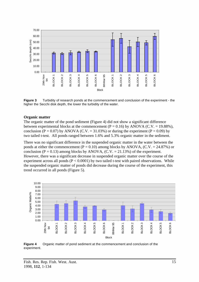
Figure 3 Turbidity of research ponds at the commencement and conclusion of the experiment - the higher the Secchi disk depth, the lower the turbidity of the water.
Organic matter The organic matter of the pond sediment (Figure 4) did not show a significant difference between experimental blocks at the commencement (P = 0.16) by ANOVA (C.V. = 19.88%), conclusion (P = 0.07) by ANOVA (C.V. = 31.03%) or during the experiment (P = 0.09) by two tailed t-test. All ponds ranged between 1.6% and 5.3% organic matter in the sediment.
There was no significant difference in the suspended organic matter in the water between the ponds at either the commencement (P = 0.10) among blocks by ANOVA, (C.V. = 24.87%) or conclusion (P = 0.13) among blocks by ANOVA, (C.V. = 21.13%) of the experiment. However, there was a significant decrease in suspended organic matter over the course of the experiment across all ponds (P < 0.0001) by two tailed t-test with paired observations. While the suspended organic matter of ponds did decrease during the course of the experiment, this trend occurred in all ponds (Figure 5).
0.001.002.003.004.005.006.007.008.009.00
10.00
29th
Nov
94
BLO
CK
1
BLO
CK
2
BLO
CK
3
BLO
CK
4
BLO
CK
5
BLO
CK
6
8thM
ar 9
5
BLO
CK
1
BLO
CK
2
BLO
CK
3
BLO
CK
4
BLO
CK
5
BLO
CK
6
Block
Org
anic
Mat
ter%
Figure 4 Organic matter of pond sediment at the commencement and conclusion of the experiment.

Fish. Res. Rep. Fish. West. Aust. 1998, 112, 1-134
16
0.00
10.00
20.00
30.00
40.00
50.00
60.00
70.00
29th
Nov
94
BLO
CK
1
BLO
CK
2
BLO
CK
3
BLO
CK
4
BLO
CK
5
BLO
CK
6
8thM
ar95
BLO
CK
1
BLO
CK
2
BLO
CK
3
BLO
CK
4
BLO
CK
5
BLO
CK
6
Blocks
Org
anic
mat
ter%
Figure 5 Suspended organic matter (%) of pond water at the commencement and conclusion of the experiment.
Yabby growth and biomass There was no significant block effect on yabby production determined as either change in biomass of adult yabbies stocked (P = 0.26) by ANOVA, total change in biomass of all yabbies harvested (including juveniles) (P = 0.50) by ANOVA, or final mean weight of yabbies (P = 0.47) by ANOVA (Figure 6). The coefficient of variation (C.V.) for yabby growth between the individual research ponds was 9.26%.
0.00
5.00
10.00
15.00
20.00
25.00
30.00
35.00
40.00
BLOCK1
BLOCK2
BLOCK3
BLOCK4
BLOCK5
BLOCK6
INITIAL
BLOCK
WEI
GH
T (g
)
Figure 6 Mean yabby weight at commencement of experiment (Initial) and variation in final yabby weights between pond blocks at conclusion of experiment (Block 1-6).
These results indicate that there was no trend across the ponds for change in yabby growth due to inherent pond factors at the site. The low variation in yabby growth (C.V. = 9.26%) between ponds treated identically showed a highly acceptable homogeneity in the pond site for future experiments.

Fish. Res. Rep. Fish. West. Aust. 1998, 112, 1-134
17
Discussion
To ensure that results of aquaculture grow-out experiments are applicable to industry, research ponds must have similar characteristics to those of industry. In addition the variation in yabby growth between ponds due to inherent site factors needs to be as small as possible to minimise the replication needed for future experiments to be effective in showing real effects due to different treatments.
The water chemistry of the Avondale research station ponds in this experiment is representative of the atypical freshwater found in the south west of WA. This atypical freshwater is dominated by the sea salt ions Na and Cl, rather than by salts from catchment erosion, such as Ca, Mg and SO4 as in other world freshwaters (Francesconi et al. 1995).
The high salinity recorded of 346 mS/m (1885 mg/L), is typical of cleared catchments in the Western Australian Wheatbelt.
Initially, the values of a number of parameters (i.e. Cl, Na, SO4-S and hardness) were higher than those recorded from most farm dams in the lower south west (Morrissy 1980) and Wheatbelt farm dams in general (Cheng et al. in prep.) (Table 2). This may be attributed to initial disturbance of the catchment due to dam construction and subsequent flushing of the catchment. However, these levels dropped during the course of experiments to well within the range experienced in Wheatbelt farm dams in Western Australia.
This experiment in the 25 research ponds at the Avondale research station demonstrated that: • The ponds behaved in a manner similar to farm dams typical of the Western Australian
Wheatbelt. The water chemistry and turbidity profiles of the ponds were within the range recorded for Wheatbelt farm dams. The percentage of organic matter in the sediments of the experimental ponds, mean 3.49%, was within the range recorded for Wheatbelt farm dams in Western Australia, which range from 0.27% to 12.13% organic matter. The 25 research ponds were therefore suitable for conducting experiments on yabby farming and the results were likely to be directly applicable to the farm dam environment; and
• The coefficient of variation between the ponds at the Avondale research station was 9.26%.
Experiments within earthen ponds at the Auburn University aquaculture research station in Alabama have produced coefficients of variation ranging from 4.2% to 34.6%, with an average of 20% (Shell 1983). Previous research using adjacent ponds for marron (Cherax tenuimanus) grow-out experiments attributed 11% of variation to differences between ponds (Morrissy 1992; Morrissy et al. 1995). Ideally the coefficient of variation should be low, since in experiments where differences are smaller than the coefficient of variation the observed differences have a high probability of being a result of chance variation rather than from a treatment effect. Comparative trials between ponds, cages and lined tanks have shown that the primary causes of variation in aquaculture production are differences in environmental conditions (water quality, productivity, soil types, water source, etc.). Furthermore, the distribution of coefficients of variation is generally similar for experiments in earthen ponds, regardless of species (Shell 1983). The comparatively low level of variation between the ponds at the Avondale research station may be attributed to a number of factors including: • The age of the facility; • The planning and design of the facility to ensure a homogeneous environment; and • The homogeneous water supply for all ponds.

Fish. Res. Rep. Fish. West. Aust. 1998, 112, 1-134
18
This experiment demonstrated that the pond site was homogeneous and, although environmental parameters such as turbidity and percentage of suspended organic matter change over time, all 25 ponds followed similar patterns of change. The ponds were therefore suitable for testing treatments, such as diet, stocking rates, mono-sex culture, etc., because any observed difference in yabby growth greater than approximately 10% shown to be the result of environmental variation, was likely to be due to the effect of the experimental treatment. References
Cheng, Y.W. and Street, D.J. 1997. Constructions for optimal non-strongly-balanced change-over designs. Comm. Stats., 26: 1073-1082.
Cheng Y.W., Lawrence C.S. and Morrissy N.M. (in prep.) To study the relationship between physical, chemical and biological parameters and yabby production in Western Australia by multiple regression.
Fisher, R.A. 1958. Statistical methods for research workers. 13th ed. Oliver and Boyd. Edinburgh, 356p.
Fisher, R.A. 1960. The design of experiments. 7th ed. Oliver and Boyd. Edinburgh, 248p. Francesconi, K.A., Morrissy, N.M., Fellows, C.J. and Bird, C. 1995. Survey of marron farms
and the marron recreational fishery in Western Australia for pesticides and water chemistry, with related laboratory experimentation. Fisheries Research Bulletin No. 30. Fisheries Department of WA, 14p.
Getchell, R.G. 1987. Effects of V-notching on the lobster, Homarus americanus. Can. J. Fish. Aquat. Sci., 44: 2033-2037.
Mann, H.B. and Whitney, D.R. 1947. On a test of whether one of two random variables is stochastically larger than the other. Ann. Math. Statist., 18: 50-60.
Morrissy, N.M. 1974. The ecology of marron Cherax tenuimanus (Smith) introduced into some farm dams near Boscabel in the Great Southern area of the Wheatbelt region of Western Australia, Fisheries Research Bulletin No. 12, Department of Fisheries and Fauna, Western Australia, 55p.
Morrissy, N.M. 1980. Production of marron in Western Australian farm dams, Fisheries Research Bulletin No. 24, Fisheries Department of WA, 80p.
Morrissy, N.M. 1984. Assessment of artificial feeds for battery culture of a freshwater crayfish, marron (Cherax tenuimanus) (Decapoda: Parastacidae. Research Report No. 63, Department of Fisheries and Wildlife, Western Australia, 43p.
Morrissy, N.M. 1992. Density-dependent pond growout of single year-class cohorts of a freshwater crayfish Cherax tenuimanus (Smith) to two years of age. J. World Aqua. Soc., 23(2): 154-168.
Morrissy, N.M., Walker, P. and Moore, W. 1995. Predictive equations for managing semi-intensive grow-out of a freshwater crayfish (marron), Cherax tenuimanus (Smith 1912) (Decapoda: Parastacidae), on a commercial farm. Aqua. Res., 26: 71-80.
Shell, E.W. 1983. Fish farming research. Auburn University, 108p. Smart, T.S., Riley, T.S. and Halyor, G. 1997. Eliminating pond differences with cross-over
designs. Aqua. Res, 28: 621-627. Wilcoxon, F. 1945. Individual comparisons by ranking methods, Biometrics Bull. 1: 80-83.
B) Density and feeding

Fish. Res. Rep. Fish. West. Aust. 1998, 112, 1-134
19
3.2 Effect of lowering density on the size of yabbies
Introduction
In general, the major problem faced when farming many species of freshwater crayfish is the production of large numbers of small animals (Avault et al. 1975; Huner and Romaire 1979; Jarboe and Romaire 1995; Morrissy 1979; Francesconi et al. 1995). In farm dams and ponds, yabbies (Cherax albidus) have multiple spawnings from early spring to mid summer. Yabbies spawn so readily, there is generally no need to purchase juveniles, with most farms producing more stock than they require. In fact the major problem faced by yabby farmers is the production of large numbers of animals which are below market size (< 30 g). (Francesconi et al. 1995; Lawrence 1998).
In freshwater crayfish such as yabbies, larger animals receive higher market prices per kilogram, this reflects the demand for larger crayfish and the greater difficulty in producing large yabbies (Lawrence 1998). Stunting of freshwater crayfish is related to population density, the higher the number of animals/m2, the lower the growth rate and the smaller the average size becomes. This has been demonstrated in a number of species including marron (C. tenuimanus) (Morrissy 1979, 1980, 1992; Morrissy et al. 1995), O. virilis (Brown et al. 1995), crawfish (P. clarki) (McClain 1995a, 1995b) and C. destructor (Geddes et al. 1995).
The most obvious cause of stunting in crayfish populations at higher densities is due to lack of food. However, Morrissy (1992) demonstrated that although the biological basis of the density-dependant growth of freshwater crayfish is that the food supply available is a result of pond area per bottom dwelling crayfish, variation in the supply of artificial feed at the demand feeding level had no apparent effect upon cohort growth. Similarly McClain (1995a) reported that weight gain of crawfish (P. clarki) was affected by density but not by feeding rate. Brown et al. (1995) also reported that feeding formulated diets to O. virilis did not give improved weight gain when reared at high densities. It has therefore been proposed that although farmers have traditionally considered that stunted crayfish were a result of lack of feed, the single most limiting factor affecting crayfish growth is population density (McClain and Romaire 1995). Whilst the exact mechanism which results in density dependent growth in crustacea has not been elucidated, it is thought to relate to a finite carrying capacity in ponds due to a number of unquantified factors which may include environment, natural food availability, deterioration of sediments, disease, social interaction, territorial restrictions or dominance hierarchies (Copp 1986; Brown et al. 1995; McClain 1995a; Maguire and Leedow 1983; Allan and Maguire 1992; Jones and Ruscoe 1996).
The impact of density is of considerable importance to a benthic animal, such as freshwater crayfish, that undergoes periods of moulting during which it is vulnerable to cannibalism (Lowery 1988). This is also likely to be true for the WA yabby C. albidus, as the closely related yabby (C. destructor) has been reported to have high intra-specific aggression and are cannibalistic (Geddes et al. 1993; Mills and McCloud 1983).

Fish. Res. Rep. Fish. West. Aust. 1998, 112, 1-134
20
Aim
The aim of two experiments was to investigate the effects of density and feeding upon farm dam populations of yabbies. In the first density experiment (Research Station Experiment 1), yabbies were stocked at two different densities and fed either the standard industry feed and feed rate per m2 or not fed (with production a result of natural food resources only). In the second density experiment (Research Station Experiment 5) yabbies were stocked at eight different densities and feed rates calculated according to the initial number and biomass of animals.
Research Station Experiment 1 Materials and methods
Twenty five 0.01 ha ponds were stocked with 7,050 juvenile yabbies (mean wt = 19.4 g, 0.22 s.e.) at either 1 or 4.5 animals/m2. Within each of these two density treatments, two lupin feeding rates were investigated, either unfed (reliant upon natural pond productivity for food resources) or fed the standard industry feed and rate of lupins at 2.5 g/m2/week. Each of the four treatment combinations was replicated six times.
In accordance with the standard reporting approach for describing freshwater crayfish growth proposed by Evans and Jussila (1997), growth rates are presented as specific growth rate (SGR).
Specific growth rate = ln (Wf)-ln(Wi)/t x 100 Where Wf = final weight, Wi = initial weight and t = time.
The experiment was stocked on 29 November 1994 and completed after 105 days on 13 March 1995. Results
There was a significant difference between the increase in the weight of unfed yabbies stocked at 1/m2 (low density) and 4.5/m2 (high density) (P < 0.001) (Table 3). Similarly there was also a significant difference between the increase in weight of fed yabbies stocked at 1/m2 (low density) and 4.5/m2 (high density) (P < 0.001) (Table 3). The SGR of unfed yabbies stocked at 1/m2 was 0.50, while at a density of 4.5/m2 it was considerably reduced at 0.08 (Table 3). Similarly while the SGR for yabbies stocked at 1/m2 and fed lupins was 0.66, the SGR for yabbies fed at the higher density of 4.5/m2 was 0.21 (Table 3). Therefore, SGR at 1/m2 for unfed yabbies is 525% greater than for the unfed higher density of 4.5/m2, and for fed yabbies the SGR 214% greater at the lower density.
Unfed yabbies grew 745% faster in low density ponds than high density ponds. Similarly fed yabbies grew 300% faster in low density fed ponds compared with high density fed ponds (Table 3). Feeding yabbies at the industry standard rate in the higher density ponds resulted in a 200% increase in growth, whilst feeding yabbies in low density ponds had a 45% increase in growth compared to unfed ponds.
Stocking density was of greater significance for yabby production than feeding lupins. Seventy-nine per cent of the growth of the yabbies could be attributed to the effect of density.
The most production in terms of adult growth and total biomass change occurred in the low density fed pond, then low density unfed, then high density fed and finally high density unfed

Fish. Res. Rep. Fish. West. Aust. 1998, 112, 1-134
21
ponds. Management practices which feed and maintain lower yabby densities can therefore result in an average weight increase of over 1,100% in comparison to unfed yabby populations at higher densities.
There was no significant difference in the survival of yabbies between densities or feeding regimes (P = 0.32) (Table 4) although the lower density and fed yabbies had a fractionally higher survival rate. Table 3 Average increase in weight per yabby at two different densities and feeding regimes over 105 days.
Density Feeding regime SGR Mean increase in s.e. (yabbies/m2) weight(g)/yabby (n = 6) 1.0 Unfed 0.50 13.43 1.1 4.5 Unfed 0.08 1.59 0.5
1.0 Lupins (2.5 g/m2/week) 0.66 19.51 1.6
4.5 Lupins (2.5 g/m2/week) 0.21 4.89 1.1
Table 4 Survival (mean±s.e., n = 6) of yabbies at two densities and feeding regimes.
Density (yabbies/m2) Survival (%) s.e. Feeding regime
4.5 58% 0.04 unfed 4.5 63% 0.06 fed 1.0 69% 0.05 unfed 1.0 68% 0.05 fed
Research Station Experiment 5 Materials and methods
Eight 0.01 ha ponds were stocked with 2,350 yabbies (mean wt = 30 g, 0.23 s.e.) at densities of 0.25, 0.5, 0.75, 1.0, 3, 5, 6, 7 yabbies/m2. In order to record the effect of density, rather than feeding, each pond was fed crayfish reference diet (CRD) at 10% initial body weight/week to ensure that feed was not limiting (Table 5). Which at an initial density of 1 yabby/m2 corresponds to feeding 20 g/m2/week. Based upon results from earlier feeding trials (section 3.4), this feed rate (20 g/m2/week) is considered to be the maximum sustainable feeding rate for a non-aerated pond. Saturation or demand feeding is not possible in farm dams, due either to a lack of aeration or an inability to observe feed in turbid water respectively. Thus, although feed/pond varied, feed/yabby was the same for all treatments. Therefore, differences in weight gain in this experiment were due to the effects of density not feed availability/animal, which otherwise would be reduced at higher stocking densities if a standard (flat) rate was applied for each treatment as in Research Station Experiment 1. The experiment was stocked on 12 February 1997 and completed after 105 days on 28 May 1997. Table 5 Density, biomass and feed rate for Research Station Experiment 5.

Fish. Res. Rep. Fish. West. Aust. 1998, 112, 1-134
22
Density Total no. of Initial Feed/wk/pond (no./m2) yabbies/pond biomass (g) (g)
0.25 25 500 50 0.5 50 1,000 100 0.75 75 1,500 150 1.0 100 2,000 200 3.0 300 6,000 600 5.0 500 10,000 1,000 6.0 600 12,000 1,200 7.0 700 14,000 1,400
Results
There was a significant difference in growth of yabbies stocked at different densities (P < 0.001). Yabbies at low densities gained more weight than yabbies at high densities. The relationship between weight gain and final density is presented in Figure 7. The growth-density relationship for yabbies in this experiment is similar to the hyperbolic relationship previously described for marron (Morrissy 1992).
0.00
10.00
20.00
30.00
40.00
50.00
60.00
70.00
0.00 0.50 1.00 1.50 2.00 2.50 3.00
FINAL DENSITY (yabbies/m2)
WEI
GH
T G
AIN
(g)
Figure 7 Weight gain of yabbies at different final densities after a 105 day grow-out period.

Fish. Res. Rep. Fish. West. Aust. 1998, 112, 1-134
23
Specific growth rate generally increased proportionately with final density (Table 6).
Table 6 Final density and specific growth rate (SGR) of yabbies.
Final SGR density 260 0.47 255 0.53 166 0.51 34 0.51 25 0.65 16 0.65 10 0.89 1 1.10
Survival was highly variable and ranged from 4% to 52% (Table 7). Table 7 Initial density, final density and survival of yabbies.
Initial density Final density Survival (no./m2) (no./m2) (%)
0.25 0.01 4 0.5 0.1 20 0.75 0.16 21 1.0 0.34 34 3.0 0.25 8.3 5.0 2.6 52 6.0 2.55 43 7.0 1.66 24
There was a slight but not significant relationship between the percentage of surviving yabbies with initial stocking density (Figure 8). There was a marked relationship between the initial and final stocking densities (Figure 9). Final stocking densities plateaued at around 2.5 yabbies/m2 (Figures 7 and 9) and may be a result of a maximum carrying capacity being reached at this level.

Fish. Res. Rep. Fish. West. Aust. 1998, 112, 1-134
24
0
10
20
30
40
50
60
0 1 2 3 4 5 6 7
INITIAL DENSITY (yabbies /m2)
SURV
IVAL
(%)
Figure 8 The relationship of yabby survival (%) to initial stocking density.
0
0.5
1
1.5
2
2.5
3
0 1 2 3 4 5 6 7
INITIAL DENSITY(yabbies/m2 )
FINA
L DE
NSIT
Y (y
abbi
es/m
2)
Figure 9 The relationship of final density at the conclusion of the experiment with initial stocking density.

Fish. Res. Rep. Fish. West. Aust. 1998, 112, 1-134
25
Discussion
The first experiment showed that the weight gain of yabbies was affected mainly by density, 79% of the growth of the yabbies could be attributed to the effect of density. Therefore, a reduction in stocking density from 4.5 to 1 yabby/m2 was more significant in increasing growth than the standard industry feeding regime. The results of the second experiment, although highly variable, indicate that yabbies, like marron, demonstrate a hyperbolic growth-density relationship even in the presence of adequate food. Therefore, the lowering of density by regular trapping and removal of yabbies will contribute more to producing larger yabbies than the current industry feeding regime using lupins at 2.5 g/m2/week. Consequently, methods to control the over-population of farm dams, due to excessive reproduction by yabbies, are likely to result in an increase in the average size of yabbies harvested as a direct result of reduced densities. Possible solutions to this problem may include mono-sex stocking, stocking of sterile yabbies, identification of strains with lower fecundity or management of farm dam populations by selective harvesting techniques. These aspects are pursued in other parts of this study. Harvesting of yabbies from farm dams follows the recommendations of Morrissy (1992), in that progressive harvesting throughout the season removes larger individuals, permitting compensatory growth by remaining yabbies. However unlike marron farming, in agricultural dams yabbies do not consist of a single year class cohort. Therefore the effect of harvesting and removal of the largest individuals whilst in the short term can be expected to produce larger yabbies, over the long term may result in a negative selection pressure, leaving smaller, slower growing animals to dominate the remaining gene pool (see section 3.7). References
Allan, G.L. and Maguire, G.B. 1992. Effects of stocking density on production of Penaeus monodon Fabricus in model farming ponds, Aquaculture, 107: 49-66.
Avault, J.W., Bretonne, L.W. and Huner, J.V. 1975. Two major problems in culturing crayfish in ponds: oxygen depletion and overcrowding. In J.W. Avault (ed.) Freshwater Crayfish II, pp. 139-144.
Brown, P.B., Wilson, K.A., Wetzel, J.E. and Hoene, B. 1995. Increased densities result in reduced weight gain of crayfish Orconectes virilis. J. World Aqua. Soc., 26(2): 165-171.
Copp, N.H. 1986. Dominance hierarchies in the freshwater crayfish Procambarus clarkii (Girard, 1852) and the question of learned individual recognition (Decapoda: Astacidea). Crustaceana, 51(1): 9-24.
Evans, L. and Jussila, J. 1987. Freshwater crayfish growth under culture conditions: Proposition for a standard reporting approach. J. World Aqua. Soc., 28(1): 11-19.
Francesconi, K.A., Bird, C., Fellows, C.J. and Morrissy, N.M. 1995. Fenvalerate as a stock management agent in extensive aquaculture for the freshwater crayfish Cherax albidus. J. Applied Aquaculture, 5(1): 11-20.
Geddes, M.C., Smallridge, M. and Clarke, S. 1993. The effect of stocking density, food type and shelters on survival and growth of the Australian freshwater crayfish, Cherax destructor, in experimental ponds. In Holdich, D.M. and Warner, G.F. (eds.) Ninth International Symposium on Astacology, pp. 57-69.
Geddes, M.C., Smallridge, M. and Clarke, S. 1995. Potential for nursery phase in the commercial production of the Australian freshwater crayfish, the yabby Cherax destructor. in Romaire, R.P (ed.) Eighth International Symposium on Astacology, pp. 504-517.

Fish. Res. Rep. Fish. West. Aust. 1998, 112, 1-134
26
Huner, J.V. and Romaire, R.P. 1979. Size at sexual maturity as a means of comparing populations of Procambarus clarkii (Gizzard) (Crustacea: Decapoda) from different habitats. In P.J. Laurent (ed.) Freshwater Crayfish, 4: 53-64.
Jarboe, H.H. and Romaire, R.P. 1995. Effects of density reduction and supplemental feeding on stunted crayfish Procambarus clarkii populations in earthen ponds. J. World Aqua. Soc., 26(1): 29-37.
Jones, C.M. and Ruscoe, I.M. 1996. Production of redclaw crayfish (Cherax quadricarinatus). FRDC Final Report Project 92/119, 154p.
Lawrence, C.S. 1998. Yabbies. In Hyde, K.(ed.) The new rural industries-A handbook for farmers and investors, pp. 147-152.
Lowery, R.S. 1988. Growth, moulting and reproduction. In Holdich, D.M. and Lowery, R.S. (eds.) Freshwater crayfish biology, management and exploitation. Timber Press Oregon 498p, pp. 83-113.
Maguire, G.B. and Leedow, M.I. 1983. A study of the optimum stocking density and feed rate for school prawns Metapenaeus macleayi (Haswell) in some Australia brackish water farming ponds. Aquaculture, 30: 285-297.
McClain, W.R. 1995a. Effects of population density and feeding rate on growth and feed consumption of red swamp crawfish Procambarus clarkii. J. World Aqua. Soc., 26(1): 14-23.
McClain, W.R. 1995b. Growth of crawfish Procambarus clarkii as a function of density and food resources. J. World Aqua. Soc., 26(1): 24-28.
McClain, W.R. and Romaire, R.P. 1995. Management considerations for the production of large procambarid crawfish. J Shellfish Res., 14(2): 553-559.
Mills, B.J. and McCloud, P.I. 1983. Effects of stocking and feeding rates on experimental pond production of the crayfish Cherax destructor Clark (Decapoda: Parastacidae).Aquaculture, 34: 51-74.
Morrissy, N.M. 1979. Experimental pond production of marron, Cherax tenuimanus (Smith) (Decapoda: Parastacidae). Aquaculture, 16: 319-344.
Morrissy, N.M. 1980. Production of marron in Western Australian Wheatbelt farm dams. Fish. Res. Bull. 24, 79p.
Morrissy, N.M. 1992. Density-dependant pond growout of single year-class cohorts of a freshwater crayfish Cherax tenuimanus (Smith) to two years of age. J. World Aqua. Soc., 23(2): 154-168.
Morrissy, N.M., Walker, P. and Moore, W. 1995. Predictive equations for managing semi-intensive grow-out of a freshwater crayfish (marron), Cherax tenuimanus (Smith 1912) (Decapoda: Parastacidae), on a commercial farm. Aquaculture Research, 26: 71-80.

Fish. Res. Rep. Fish. West. Aust. 1998, 112, 1-134
27
3.3 Feeding lupins at the current industry standard rate vs non feeding Introduction
The yabby industry in Western Australia at the start of this study was based upon supplementary feeding of lupins (Lupinus albus) to yabbies in farm dams. Although feeding times, dam size and feed rates varied, the average feeding regime reported by farmers was lupins at the rate of 2.5 g/m2/week.
Although the developing yabby industry rapidly adopted the feeding of lupins, there was no scientific evidence available to support this supplementary feeding regime. Most of the feed of yabbies in farm dams is thought to be derived from natural sources and feed chains, which are known to support a biomass of approximately 400 kg/ha/year (N. Morrissy pers. comm. 1998). Aim
The aim of this first experiment was to measure the effect of supplementary feeding of lupins upon the growth of yabbies. Research Station Experiment 1 Materials and methods
This experiment was nested with density and variation between ponds (sections 3.1 and 3.2). Twenty five 0.01 ha ponds were stocked with 7,050 yabbies (mean wt = 19.4 g, 0.22 s.e.) at an initial stocking density of either 4.5 or 1 yabby/m2. The control was unfed, reliant upon natural dam productivity for food, which was compared with the standard industry supplementary feeding regime of lupins at a rate of 2.5 g/m2/week. In addition the effect of feeding yabbies stocked at a higher density (4.5/m2) was tested. The control and treatments were replicated six times. The SGR was calculated according to the method presented previously (section 3.2). The food conversion ratio (FCR; where FCR = food fed/weight gain) was calculated. The experiment was stocked on 29 November 1994 and completed after 105 days on 13 March 1995. Results
There was a significant difference between the increase in the weight of yabbies fed lupins compared with the unfed control (P < 0.05) (Table 8).
Table 8 Average increase in weight for fed and unfed yabbies at two densities over 105 days.
Treatment Mean increase in weight s.e. % increase in weight (g/yabby) (n = 6) compared to control Control (unfed 1.0 yabbies/m2) 13.43 1.1 0 Fed (1.0 yabbies/m2) 19.51 1.6 45 Unfed (4.5 yabbies/m2) 1.59 0.5 -88 Fed (4.5 yabbies/m2) 4.89 1.1 -64
At a density of 1 yabby/m2 yabbies fed lupins at the industry standard rate were on average 6 g larger, representing an increase in mean weight of 45% over unfed animals during the period of this experiment (Table 8). However, it should be noted from Table 6 that unfed yabbies stocked at 1/m2 increased in size by 13 g, thus natural food production in ponds was responsible for 69% of the growth in this treatment.

Fish. Res. Rep. Fish. West. Aust. 1998, 112, 1-134
28
At higher densities (4.5 yabbies/m2), the increase in weight in the treatment fed lupins was over 200% greater than for unfed yabbies at the same density. However, at this higher density the proportion of yabby growth from natural food production was only 33%. Therefore the benefits gained from feeding lupins are greater at higher densities, probably as a result of the amount of natural food available in the farm dam becoming limiting.
This supports the results in section 3.2 where stocking density was shown to be of greater significance to yabby production in the experimental dams than feeding lupins. It was found that 79% of the growth of the yabbies could be attributed to the effect of density and 21% to the effect of feeding lupins (section 3.2).
Survival is presented in Table 9. There was no significant difference in survival due to feeding (P = 0.32).
Table 9 Survival of yabbies at two densities and feeding regimes.
Feeding Density Survival Ponds regime (yabbies/m2) (n) Unfed 1.0 69% 6 Fed 1.0 68% 6 Unfed 4.5 58% 6 Fed 4.5 63% 6
In the lower density treatment the addition of 3,750 g of lupins per pond over the experimental period resulted in an average increase of 19.51 g (1.60 s.e.) per surviving yabby (Table 8). This equates to an FCR of 2.83. At the higher density of 4.5 yabbies/m2, although growth was less (4.89 g/yabby) the higher total number of yabbies resulted in a slightly improved FCR of 2.74. The FCR does not include natural food, which has been shown in this experiment, particularly at low densities, to provide a significant contribution to yabby growth. Therefore, while these FCRs are useful for demonstrating relative efficiency of feeding, suitable for comparison within this experiment, these apparently low values probably underestimate the true food consumption of crayfish which is actually the sum of supplementary feed + natural feed consumed.
The specific growth rate (SGR) of unfed yabbies at 1/m2 which relied upon natural pond production for food resources was 0.50, while the SGR for yabbies fed lupins was 0.66, representing an increase in growth rate of 32%. SGR for yabbies was considerably lower at the higher density of 4.5/m2. The SGR of unfed yabbies at a density of 4.5/m2 was 0.08 and fed yabbies at the same density was 0.21, representing an increase in growth rate due to feeding of 162%. Discussion
The addition of lupins provided increased yabby growth. However, density had a much greater effect upon growth than the current industry feeding regime (section 3.2). Food appears to be limiting yabby growth particularly at high densities. However, it is not known whether yabbies are consuming lupins directly or the lupins contribute to the natural food chains. Comparison of fed and unfed yabbies demonstrated that up to 69% of the growth of yabbies in industry farm dams can be attributed to the consumption of naturally occurring food sources. The benefits gained from feeding lupins are greater at higher

Fish. Res. Rep. Fish. West. Aust. 1998, 112, 1-134
29
densities, probably as a result of the amount of natural food available in the farm dam becoming limiting. Therefore, density and feed are important and limiting in yabby ponds - density more so - and highly interactive as would be expected. Management practices which feed and maintain lower yabby densities can therefore result in an average weight increase of over 1,100% in comparison with unfed yabby populations at higher densities.
3.4 Effect of increased feed rates and alternative feeds on growth of yabbies Introduction
The previous trial indicated that yabbies give additional growth on the standard industry feeding rate for lupins. However, the lupin diet may be limited by either the quality or quantity of nutrients. The previous experiment suggested a series of experiments, designed to evaluate various low cost readily available alternative food sources considered by industry to show potential for yabby farming, was necessary. As well, increased feed rates were evaluated to investigate whether the quantity of feed was limiting yabby growth.
Growth of yabbies is highly dependant upon temperature and hence the time of year when the experiment is conducted. For this reason, a standard control diet (lupins 2.5 g/m2 at a density of 1 yabby/m2) was maintained in all experiments to: i) permit relative efficiencies and growth to be estimated; and ii) investigate the seasonal variation of growth of yabbies both within years and between
years.
The food conversion ratio (FCR) and specific growth rate (SGR) were calculated for each experiment according to the methods presented previously in sections 3.2 and 3.3.
Proximate analyses for all diets evaluated are presented in Appendix 4.
3.4.1 Increased lupin feed rate vs CRD (Research Station Experiment 2)
Aim
This experiment compared the standard industry feeding rate for lupins with an increased feeding rate of lupins. The experiment also investigated the effectiveness of using a pelletised crayfish reference diet (CRD) for feeding yabbies. The CRD was developed to provide a standardised control diet, based upon an open formulation, which researchers could use as a basis for future feed evaluation experiments for freshwater crayfish (Morrissy 1989, 1992). Lupins, due to their low cost (35-40 c/kg) and ready availability to farmers, have been used by industry to feed yabbies. The CRD is a more complete, low cost (56 c/kg), formulated diet including fish, meat and blood meal, but still considered incomplete as a sole diet for crayfish. The CRD contains 18% animal based protein and 3% vegetable protein, whereas lupins contain around 28% vegetable protein (Appendix 4). Materials and methods
Eighteen ponds were stocked with 1,800 yabbies at an initial density of 1/m2, similar to that of a farm dam. The mean initial stocking weight of yabbies was 19.54 g (0.19 s.e.). Six replicates of three feeding regimes were stocked in 18 ponds according to the following treatments: lupins standard rate = 2.5 g/m2/week; lupins double rate = 5.0 g/m2/week; and CRD at 2.5 g/m2/week.

Fish. Res. Rep. Fish. West. Aust. 1998, 112, 1-134
30
The experiment was stocked on 26 July 1995 and completed after 175 days on 16 January 1996. All yabbies were removed from ponds and individually sexed and weighed. Results
The survival data expressed as the proportion of original yabbies surviving were transformed prior to using analysis of variance to satisfy the assumption of normality. The arcsine square root transformation was used.
There was no significant difference in survival between feed treatments (Table 10, P = 0.31). Therefore, growth differences recorded in this experiment can be considered to be due to the different feed treatments, not the effect of density. Table 10 Survival for the six treatments.
Treatment Sex Survival (%) s.e. n Control lupins (2.5 g/m2/week) female 42 - 1 Control lupins (2.5 g/m2/week) male 69 13.0 2 Control lupins (2.5 g/m2/week) mixed-sex 79 4.50 2 Lupins (5 g/m2/week) female 88 5.50 2 Lupins (5 g/m2/week) male 71 4.00 2 Lupins (5 g/m2/week) mixed-sex 75 11.0 2 Crayfish reference diet (2.5 g/m2/week) female 85 15.0 2 Crayfish reference diet (2.5 g/m2/week) male 69 9.00 2 Crayfish reference diet (2.5 g/m2/week) mixed-sex 56 13.0 2
There was a significant difference in yabby growth between the three feed treatments (P < 0.05) (Table 11). A least significant difference (LSD) test revealed that the mean weight gains for the lupin 2.5 g/m2 and CRD 2.5 g/m2 treatments were significantly different, although the lupin 5 g/m2 diet was not significantly different from the others (Table 11).
Table 11 Mean weight increase for three feeding regimes (means sharing the same subscript letter are not significantly different P > 0.05).
Treatment Mean increase in s.e. Increase in weight weight (g/yabby) compared to control (%) Control lupins 28.2a 3.38 0
(2.5 g/m2/week) Lupins (5 g/m2/week) 32.1ab 4.10 14 Crayfish reference diet 33.9b 4.48 20
(2.5 g/m2/week)
Therefore, although a 100% increase in the feed rate of lupins did provide a slight increase in weight gain (14%), this was not significant statistically. The CRD was a more efficient food source, providing a significant increase in growth (20%) when compared with lupins at the same feeding rate (2.5 g/m2/week).
Furthermore, the results of this experiment demonstrate that it only requires half as much CRD to achieve the same growth as lupins. CRD is therefore considered to be twice as efficient a diet for yabbies as lupins. This is particularly significant in farm dams, as these

Fish. Res. Rep. Fish. West. Aust. 1998, 112, 1-134
31
waterbodies are undrainable and do not have mechanical aeration. They are therefore more susceptible to eutrophication through over-feeding than semi-intensive fish ponds. CRD returned the lowest food conversion ratio and increasing lupin feeding rates resulted in less efficient use of this feed (Table 12). Table 12 Food conversion ratios (FCR) for three feeding regimes.
Diet FCR Lupins (2.5 g/m2/week) 3.31 Lupins (5 g/m2/week) 4.99 Crayfish reference diet (2.5 g/m2/week) 2.63
As observed previously in section 3.3 the FCRs are likely to be underestimates of the true FCRs as they do not take into account natural food production or cannibalism.
The specific growth rate (SGR) of CRD fed at 2.5 g/m2/week is 14% greater than lupins at the same feed rate. Furthermore the SGR of CRD fed at 2.5 g/m2/week is greater than that of lupins fed at 5 g/m2/week. Twice as much lupin is needed to achieve a similar specific growth rate as CRD (Table 13).
Table 13 Specific growth rates (SGR) for three feeding regimes.
Diet SGR Increase in SGR compared to control (%) Lupins (2.5 g/m2/week) 0.51 0 Lupins (5 g/m2/week) 0.55 8 Crayfish reference diet
(2.5 g/m2/week) 0.58 14
Conclusions
Results from the previous trials have indicated that feeding lupins to yabbies at the industry standard rate of 2.5 g/m2/week, depending upon density, provided between 45% and 200% improved growth over not feeding at all. Increasing the lupin feeding rate from 2.5 g/m2/week to 5 g/m2/week provided increased growth (14%), however this was not significant at the P = 0.05 level. The CRD diet fed at 2.5 g/m2/week provided significantly improved growth (20%) over feeding lupins at 2.5 g/m2/week, and improved, though not significant, growth (6%) compared with lupins at 5 g/m2/week.

Fish. Res. Rep. Fish. West. Aust. 1998, 112, 1-134
32
3.4.2 Increased lupin feed rate vs CRD vs meat (Research Station Experiment 3)
Aim
The aim of this experiment was to determine whether further increases in feed rates of lupins and crayfish reference diet (CRD) increased growth. In addition, the feeding of meat was tested. Materials and methods
Twelve experimental 0.01 ha ponds were used. Each pond was drained after the previous experiment then refilled. All 12 ponds were stocked at the same density of 1/m2. The mean weight of yabbies stocked was 25.92 g (0.40 s.e.). The experiment compared four feeding regimes as follows: i) lupins at 2.5 g/m2 for 1 yabby/m2 was retained as a control; ii) lupins at 10 g/m2/week, which is four times the industry average feeding rate; iii) CRD at 10 g/m2/week; and iv) meat at 10 g/m2/week. The experimental ponds were stocked on 22 January 1996 and completed after 108 days on 8 May 1996. Results
There was a significant difference in the mean weight gain of yabbies between diet treatments (P < 0.0001) (Table 14). CRD provided improved growth.
Table 14 Mean weight increase for four feeding regimes.
Treatment Mean increase in weight s.e. Increase in weight (g/yabby) (n = 3) compared to control (%) Control lupins
(2.5 g/m2/week) 15.19 1.38 0 Lupins (10 g/m2/week) 21.14 1.56 39 Meat (10 g/m2/week) 19.88 1.54 31 Crayfish reference diet
(10 g/m2/week) 27.99 1.07 84
In comparison with the control diet, yabbies fed lupins at 10 g/m2/week grew an additional 39%, while yabbies fed CRD grew 84% more than the control.
Feed was utilised less efficiently with increasing rates of feeding. At the higher feeding rate of 10 g/m2/week the CRD diet provided the best FCR (Table 15).
Table 15 Food conversion ratios (FCR) for four feeding regimes.
Treatment FCR Lupins (2.5 g/m2/week) 3.06 Lupins (10 g/m2/week) 9.10 Meat (10 g/m2/week) 11.03 Crayfish reference diet (10 g/m2/week) 6.76

Fish. Res. Rep. Fish. West. Aust. 1998, 112, 1-134
33
Growth rate increases with increased feed rate additions (Table 16). Of the three feeds in this experiment, CRD gave the highest SGR and is 58% faster than the current industry standard feeding regime. Table 16 Specific growth rates (SGR) for four feeding regimes.
Treatment SGR Increase in SGR compared to control (%) Lupins (2.5 g/m2/week) 0.43 0 Lupins (10 g/m2/week) 0.55 28 Meat (10 g/m2/week) 0.53 23 Crayfish reference diet (10 g/m2/week) 0.68 58
Survival was relatively high and similar across all the treatments, ranging from 72% to 87% (Table 17). Table 17 Survival for the four feeding treatments.
Treatment Survival (%) s.e. n Crayfish reference diet (10 g/m2/week) 80 3.18 3 Lupins (10 g/m2/week) 82 4.04 3 Lupins (2.5 g/m2/week) 87 3.71 3 Meat (10 g/m2/week) 72 9.26 3
Conclusions
Increased feeding rates of lupins resulted in an additional 39% increase in the weight of yabbies compared with the industry control diet. Increased feeding rates of CRD gave an additional 84% increase in the weight of yabbies, when compared with the industry control diet.
3.4.3 Increased CRD feed rates (Research Station Experiment 4)
Aim
Three feeding rates were tested to confirm the increased growth on crayfish reference diet (CRD) and to determine the upper range of feeding before growth rates declined due to degradation of environmental conditions. Materials and methods
Twelve ponds each 0.01 ha in size were used. The 12 ponds were stocked at a density of 1 yabby/m2. The initial stocking weight of yabbies was 25.36 g (0.30 s.e.).
Four feeding regimes each replicated three times were evaluated in this trial. 1) The control diet of Lupin 2.5 g/m2/week was retained. 2) Three CRD feed rates were tested:
a) 10 g/m2/week; b) 20 g/m2/week; and c) 30 g/m2/week.

Fish. Res. Rep. Fish. West. Aust. 1998, 112, 1-134
34
The experiment was stocked on 8 October 1996 and completed after 100 days on 15 January 1997. Results
There was a significant difference in the mean weight gain of yabbies between diet treatments (P < 0.05) (Table 18). CRD at 20 g/m2/week provided the largest mean weight gain (66%) for yabbies in this experiment (Table 18).
Table 18 Mean weight increase for four feeding regimes.
Treatment Mean increase in weight s.e. Increase in weight (g/yabby) (n = 3) compared to control (%) Control lupins (2.5 g/m2/week) 23.24 0.99 0 CRD (10 g/m2/week) 32.51 0.95 40 CRD (20 g/m2/week) 38.61 2.19 66 CRD (30 g/m2/week) 35.09 1.24 51
Although CRD provided increased growth at 20 g/m2/week, less growth was achieved when feeding at 30 g/m2/week. It is therefore possible that at higher application rates CRD is utilised increasingly inefficiently and/or that the yabbies were being over fed at the feed rate of 30 g/m2/week(Table 19). Table 19 Food conversion ratios (FCR) for four feeding regimes.
Treatment FCR Lupins (2.5 g/m2/week) 2.11 CRD (10 g/m2/week) 6.59 CRD (20 g/m2/week) 9.87 CRD (30 g/m2/week) 18.98
Specific growth rate was highest at feeding CRD at the rate of 20 g/m2/week, and is 43% greater than the industry standard feeding regime of lupins at 2.5 g/m2/week, but the highest feed rate of CRD at 30 g/m2/week resulted in a lower SGR than 20 g/m2/week (Table 20).
Table 20 Specific growth rates (SGR) for four feeding regimes.
Treatment SGR Increase in SGR compared to control (%) Lupins (2.5 g/m2/week) 0.65 0 CRD (10 g/m2/week) 0.83 28 CRD (20 g/m2/week) 0.93 43 CRD (30 g/m2/week) 0.87 34

Fish. Res. Rep. Fish. West. Aust. 1998, 112, 1-134
35
Survival was high and similar across all treatments (Table 21).
Table 21 Survival for the four feeding treatments.
Treatment Survival(%) s.e. n Lupins (2.5 g/m2/week) 82 7.62 3 Crayfish reference diet (10 g/m2/week) 75 7.26 3 Crayfish reference diet (20 g/m2/week) 63 21.84 3 Crayfish reference diet (30 g/m2/week) 72 8.09 3
It should be noted from Tables 18 and 20 (Research Station Experiment 4) and Tables 14 and 16 (Research Station Experiment 3), that the per cent increase in both weight and SGR for CRD at 10 g/m2/week compared with the control were lower in Research Station Experiment 4. As the SGR for both the control and CRD (10 g/m2/week) was in fact higher in Research Station Experiment 4 than Research Station Experiment 3, the reduced percentage increase may, in fact, be a result of improved growth in the control diet due to annual or seasonal variation in natural food production; which has been shown to have a significant contribution to yabby growth (section 3.3).
Alternatively the variation recorded may be due to as yet undetermined factors which are the focus of a current experiment or may indicate that these higher feeding rates are not sustainable in the farm dam environment over the longer-term. Conclusions
Feeding CRD provided increased weight gain, in comparison with the industry control diet, up to a feeding rate of 20 g/m2/week. Growth plateaued at the higher feed rate of 30 g/m2/week, most probably due to over-feeding which results in poor water quality.
3.4.4 Low cost industry diets (Research Station Experiment 5)
Introduction
Industry encourages the use of readily available cheap farm produce for feeding yabbies. The feeds selected for this experiment were already being used by farmers. However, the effectiveness of these feeds in enhancing yabby growth had not been quantified.
It has been shown that a significant proportion of yabby feed is derived from natural productivity in farm dams (section 3.3). Although a fertiliser has not been used by yabby farmers in WA, this is used internationally to stimulate natural productivity in aquaculture ponds. Aim
The aims were to investigate and compare: i) low cost feeds used by farmers (i.e. lupins, wheat, oats, barley and meat meal); ii) any difference between feeding whole or rolled lupins (i.e. are the yabbies eating the
sprouts from whole lupins); and iii) if inorganic fertilisers stimulate natural food production as effectively as current
industry feeds for yabbies.
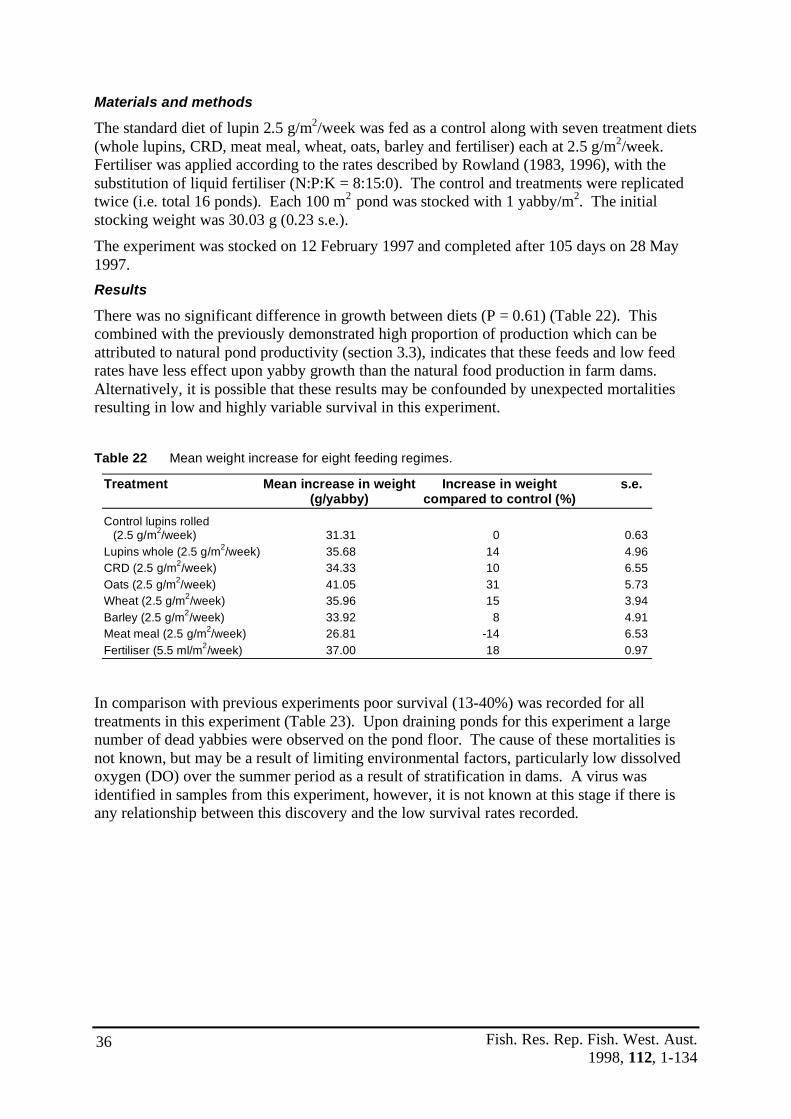
Fish. Res. Rep. Fish. West. Aust. 1998, 112, 1-134
36
Materials and methods
The standard diet of lupin 2.5 g/m2/week was fed as a control along with seven treatment diets (whole lupins, CRD, meat meal, wheat, oats, barley and fertiliser) each at 2.5 g/m2/week. Fertiliser was applied according to the rates described by Rowland (1983, 1996), with the substitution of liquid fertiliser (N:P:K = 8:15:0). The control and treatments were replicated twice (i.e. total 16 ponds). Each 100 m2 pond was stocked with 1 yabby/m2. The initial stocking weight was 30.03 g (0.23 s.e.). The experiment was stocked on 12 February 1997 and completed after 105 days on 28 May 1997. Results
There was no significant difference in growth between diets (P = 0.61) (Table 22). This combined with the previously demonstrated high proportion of production which can be attributed to natural pond productivity (section 3.3), indicates that these feeds and low feed rates have less effect upon yabby growth than the natural food production in farm dams. Alternatively, it is possible that these results may be confounded by unexpected mortalities resulting in low and highly variable survival in this experiment.
Table 22 Mean weight increase for eight feeding regimes.
Treatment Mean increase in weight Increase in weight s.e. (g/yabby) compared to control (%) Control lupins rolled
(2.5 g/m2/week) 31.31 0 0.63 Lupins whole (2.5 g/m2/week) 35.68 14 4.96 CRD (2.5 g/m2/week) 34.33 10 6.55 Oats (2.5 g/m2/week) 41.05 31 5.73 Wheat (2.5 g/m2/week) 35.96 15 3.94 Barley (2.5 g/m2/week) 33.92 8 4.91 Meat meal (2.5 g/m2/week) 26.81 -14 6.53 Fertiliser (5.5 ml/m2/week) 37.00 18 0.97
In comparison with previous experiments poor survival (13-40%) was recorded for all treatments in this experiment (Table 23). Upon draining ponds for this experiment a large number of dead yabbies were observed on the pond floor. The cause of these mortalities is not known, but may be a result of limiting environmental factors, particularly low dissolved oxygen (DO) over the summer period as a result of stratification in dams. A virus was identified in samples from this experiment, however, it is not known at this stage if there is any relationship between this discovery and the low survival rates recorded.

Fish. Res. Rep. Fish. West. Aust. 1998, 112, 1-134
37
Table 23 Survival for eight feeding regimes.
Treatment Survival (%) s.e. n Lupins rolled (2.5 g/m2/week) 13 0.09 2 Lupins whole (2.5 g/m2/week) 22 0.01 2 CRD (2.5 g/m2/week) 28 0.11 2 Oats (2.5 g/m2/week) 40 0.10 2 Wheat (2.5 g/m2/week) 22 0.00 2 Barley (2.5 g/m2/week) 24 0.01 2 Meat Meal (2.5 g/m2/week) 28 0.09 2 Fertiliser (5.5 ml/m2/week) 34 0.09 2
Table 24 Food conversion ratios (FCR) for eight feeding regimes.
Treatment FCR Lupins rolled (2.5 g/m2/week) 6.84 Lupins whole (2.5 g/m2/week) 6.18 CRD (2.5 g/m2/week) 3.90 Oats (2.5 g/m2/week) 2.31 Wheat (2.5 g/m2/week) 4.97 Barley (2.5 g/m2/week) 4.61 Meat meal (2.5 g/m2/week) 4.99 Fertiliser N/A
Table 25 Specific growth rates (SGR) for eight feeding regimes.
Treatment SGR Increase in SGR compared to control (%) Lupins rolled (2.5 g/m2/week) 0.68 0 Lupins whole (2.5 g/m2/week) 0.73 7 CRD (2.5 g/m2/week) 0.73 7 Oats (2.5 g/m2/week) 0.82 21 Wheat (2.5 g/m2/week) 0.75 10 Barley (2.5 g/m2/week) 0.72 6 Meat meal (2.5 g/m2/week) 0.61 -10 Fertiliser (5.5 ml/m2/week) 0.76 12
The increase in weight, survival and SGR of the liquid fertiliser treatment (Tables 22, 23 and 25), show that this treatment, which cannot be consumed directly by the yabbies, is comparable to the addition of supplementary feeds. This result lends support to the hypotheses that yabbies do not directly consume the food which is being added to farm dams. Instead, current supplementary feeding practices feed the farm dam ecosystem, thus increasing the natural food resources for yabbies. There are, however, a number of mechanisms by which fertiliser can affect growth (i.e. feed, water quality), this is the focus of current experiments designed to elucidate the function of feed in the farm dam environment. Conclusions
The low value feeds compared in this experiment, combined with relatively low feed rates provided only small increases in yabby weight. Of the low cost industry supplementary feeds, oats provided the best growth.
The survival in this experiment may have been reduced due to other, as yet unidentified, factors.

Fish. Res. Rep. Fish. West. Aust. 1998, 112, 1-134
38
3.4.5 Variation in lupin control (Research Station Experiments 1-5)
Aim
A control diet of lupins fed at the rate of 2.5 g/m2/week was included in all experiments to determine the amount of variation in yabby growth between experiments. Weight gain data from each experiment was expressed as a specific growth rate (SGR). SGRs express the increase in yabby weight relative to initial weight based upon a log (curved) model.
In a recent review, Evans and Jussila (1997) recommended that SGR should be used to provide a standard reporting approach for crayfish growth experiments. SGRs are therefore included to permit comparison by other freshwater crayfish researchers. Materials and methods
The SGR was calculated for each of the lupin 2.5 g/m2/week controls in each experiment according to the methods presented previously in section 3.3 as:
Specific growth rate (SGR) = ln (Wf)-ln(Wi)/t x 100 Where Wf = final weight, Wi = initial weight and t = time.
Results
Specific growth rates were similar for all experiments, except for Research Station Experiments 2 and 3 which were slightly lower (Table 26). Table 26 SGR for the controls in five research station experiments.
Experiment Wi Wf d SGR s.e. Water Temp Range (0C) 1 19.4 38.91 105 0.66 0.03 19-27 2 19.54 47.74 175 0.51 0.02 18-27 3 25.92 41.11 108 0.43 0.04 25-26 4 25.36 48.6 100 0.65 0.01 20-27 5 30.03 61.34 105 0.68 0.01 18-26
Research Station Experiment 2 was stocked during winter in July 1995. As the growth of yabbies is related to water temperature, the reduced SGR in Experiment 2 is likely to be due to the effect of lower winter/spring water temperatures being limiting. This may be either a result of temperature directly limiting growth or indirectly reducing pond productivity and consequently naturally occurring food resources. These results highlight the difficulty of attempting to compare freshwater crayfish grow-out experiments that are conducted over different periods of time, in particular seasons, as SGRs are affected by variations in temperature.
The reason for the reduced growth in Experiment 3 is unknown at this stage. In comparison to the other four experiments the most obvious difference in Experiment 3 was that the ponds were not allowed to dry out between Experiment 2 and Experiment 3. After draining, the ponds were refilled and stocked within a six-day period. The other experiments ranged from a minimum of 28 to a maximum of 155 days between experiments. Alternatively the reduced SGR in Experiment 3 may be a result of a carry over effect, limiting environmental factors, or seasonal variations between years.

Fish. Res. Rep. Fish. West. Aust. 1998, 112, 1-134
39
However the reduced SGR in Experiment 3 does indicate that growth of the treatments in this experiment may have been underestimated. This supports the higher SGR obtained for CRD (10 g/m2/week) in Experiment 4 (0.83) (Table 20), compared with 0.68 (Table 16) in Experiment 3. Conclusion
Growth rates for controls in all experiments were less than 1% per day. Growth rates were similar for Experiments 1, 4 and 5, but were slightly lower for Experiments 2 and 3. While Evans and Jussilla (1997) observed that SGRs tended to be higher for longer studies, they proposed that this was due to the age of the crayfish in the experiments. This is based upon the findings of Hartnoll (1982) that growth rates decrease with increase in size. The results of this experiment do not show a clear relationship between SGR and initial weight. The lower SGRs in longer experiments, such as Experiment 2, may also be due to reduced growth if experiments extend past the optimal growing period into winter. Consequently SGRs which are not corrected for temperature are more useful for comparing experiments that run for an entire year or experiments run during the same season and period in years with similar temperatures. The issue of variation in growth rates due to temperature has been discussed by Morrissy (1990, 1992), who recommends that a correction factor for temperature should be included in growth studies of freshwater crayfish. General discussion
This series of experiments has demonstrated that improved feeds and feed rates can result in increased mean weight gain and therefore an increased proportion of yabbies that are of market size.
The maximum growth was achieved feeding CRD at the rate of 20 g/m2/week. However, it is unlikely that this relatively high feeding rate is sustainable and economically viable in the farm dam environment, which does not have mechanical paddle wheel aeration. The maximum feeding rate for CRD in paddle wheel aerated marron ponds is 35 g/m2/week (Morrissy pers. comm., Boyd pers. comm.) CRD is a suitable reference diet for yabbies and it is therefore recommended as a control diet for future evaluation of yabby feeding and management regimes. The SGR of the control treatment for five separate experiments over a period of three years ranged from 0.47 to 0.68 (Table 26). The use of SGR as an indicator of yabby growth has some limitations when attempting to compare growth between experiments. The use of a standard control diet has shown that specific growth rate varies between experiments conducted at different times of the year. It is known that yabby growth and reproduction is related to temperature; and it has also been shown previously (section 3.2) that a significant proportion of food in farm dams is derived from natural productivity which may vary according to environmental parameters such as temperature, photoperiod, nutrients and season. SGR does however provide a useful method for comparing growth rates between treatments within experiments and between experiments of similar duration.

Fish. Res. Rep. Fish. West. Aust. 1998, 112, 1-134
40
References
Evans, L. and Jussila, J. 1987. Freshwater crayfish growth under culture conditions: Proposition for a standard reporting approach . J. World Aqua. Soc., 28(1): 11-19.
Hartnoll, R.G. 1982. Growth. In Abele, L.G. (ed.) The Biology of Crustacea, Academic Press: New York, 2: 111-196.
Morrissy, N.M. 1982. A standard reference diet for crustacean nutrition research. IV: Growth of freshwater crayfish Cherax tenuimanus. J. World Aqua. Soc., 20(3): 114-117.
Morrissy, N.M. 1990. Optimum and favourable temperatures for growth of Cherax tenuimanus (Smith 1912) (Decapoda: Parastacidae), Aust. J. Mar. Freshwater Res., 41: 735-746.
Morrissy, N.M. 1992. Feed development for marron Cherax tenuimanus, in Western Australia. In Allan, G.L. and Dall, W. (eds.), Proc. Aquaculture Nutrition Workshop, Salamander Bay, 15-17 April 1991.,. NSW Fisheries, pp. 72-76.
Rowland, S.J. 1983. The hormone-induced spawning and larval rearing of Australian native freshwater fish, with particular emphasis on the golden perch, Macquaria ambigua. Proceedings of the 1st Freshwater Aquaculture Workshop, pp. 23-32.
Rowland, S.J. 1996. Development of techniques for the large-scale rearing of the larvae of the Australian freshwater fish Golden Perch, Macquaria ambigua (Richardson, 1845) Mar. Freshwater Res. 47: 233-242.
C) Mono-sex culture 3.5 Effect of single sex grow-out on size of male and female yabbies Introduction
Poor growth of yabbies (Cherax albidus) reduces the value of farm dam crayfish production, since the price received per kg for crayfish is directly related to the individual weight of the animals. There are several mechanisms, other than food supply, that may limit the growth of crayfish and, hence, lead to stunting at increased densities, such as increased energy requirements to compete for food, or diversion of energy from somatic growth to reproductive effort (i.e. competition for mates and production of gametes). Female crayfish develop large yolky eggs and the effect of this reproductive effort can be observed in female yabbies, which grow at the same rate as males until sexual maturity at about 20 g, after which, relative to males, female growth slows markedly (Woodland 1967). The yabby is an r-selected species and consequently has the potential to produce large numbers of offspring by repeated spawning each season and/or at an early age and size (Stearns 1976; Faragher 1983; Lake and Sokol 1986). If population growth is uncontrolled by mortality due to periodic drought, yabbies can rapidly reach a population density where growth of individuals is greatly reduced.
One way to control population density is to prevent reproduction. However, juvenile yabbies are produced over the warmer months of the year (September-May) by broodstock contained within farm dams where there is currently little or no control by harvesters over yabby reproduction or density. If farm dams were to be stocked with single sex individuals, however, then reproduction would not occur and density could not increase.

Fish. Res. Rep. Fish. West. Aust. 1998, 112, 1-134
41
Controlling reproductive effort and density with single sex individuals has been shown to be an effective way of increasing production in other freshwater crustaceans; e.g. mono-sex culture of the freshwater prawn M. rosenbergii, has demonstrated increased average weights for male populations in comparison to mixed-sex or female-only populations (Sagi et al. 1986; Cohen et al. 1988). Mono-sex culture of the tropical Australian freshwater crayfish redclaw (C. quadricarinatus) by Curtis and Jones (1995), demonstrated improved growth rate for male-only populations (1.12 g/week) over mixed-sex populations (0.52 g/week) and female only populations (0.27 g/week). In their experiment, reproduction occurred in ponds and the increased growth rate in all-male populations compared to all-female and mixed-sex cultivation was attributed to changes in density and retardation of female somatic growth due to the onset of sexual maturity. Aim
This research was aimed at evaluating the potential of single sex production as a method for producing larger yabbies. Materials and methods
Eighteen 0.01 ha ponds were stocked with yabbies at an initial density of 1/m2. Prior to stocking, the yabbies were sexed by manual examination for the presence of penes at the base of the fifth pair of periopods for males, or gonopores at the base of the third pair of periopods for females. Inter-sex animals were excluded from the study. A completely randomized block design with two factors, sex and diet, was used. Factor sex had three levels, male (M), female (F) and mixed-sex (A, 1:1 ratio). Factor diet had three levels, lupin (Lupinus albus) at 2.5 g/m2/week (L250), lupin (Lupinus albus) at 5.0 g/m2/week (L500), and crayfish reference diet at 2.5 g/m2/week (C250). There were two blocks. A random sample of yabbies was weighed prior to stocking each treatment. The mean stocking weight of yabbies in this experiment was 19 g (0.19 s.e.) (n = 180). The ponds were stocked in July 1995 and harvested after 175 days so as to include five months of the yabby breeding season. All yabbies were then harvested by trapping and then draining the ponds to collect the remaining animals. Immediately after harvesting all yabbies were individually sexed and weighed. Production of juveniles occurred in mixed-sex ponds. A small number of juveniles were also found in some mono-sex ponds. As yabbies have previously been recorded to mature at 20 g, it is possible that some females had mated prior to stocking (Woodland 1967).
Construction of weight frequency histograms, showed cohorts of juveniles from reproduction in ponds during the experiment as animals with weights below the initial stocking weights; these animals could therefore be identified during the analyses of the data. Results
Size frequency distribution In comparison with female and mixed-sex ponds, those stocked with only male yabbies resulted in a greater proportion of animals in the larger size classes at harvest for each diet treatment. The frequency distribution of adult yabbies in each pond is shown in Figures 10, 11 and 12.

Fish. Res. Rep. Fish. West. Aust. 1998, 112, 1-134
42
0 20 40 60 80 100
010
2030
40
FL250
increased body weight (g)
0 20 40 60 80 100
010
2030
40
FL500
final body weight (g)
0 20 40 60 80 100
010
2030
40
C250
final body weight (g)
0 20 40 60 80 100
010
2030
40
FL250
final body weight (g)
0 20 40 60 80 100
010
2030
40FL500
final body weight (g)
0 20 40 60 80 1000
1020
3040
C250
final body weight (g)
Figure 10 The frequency distribution of six ponds with female yabbies from different diet treatments (juveniles have been excluded), where F = female; C250 = CRD 2.5 g/m2/week; L250 = lupin 2.5 g/m2/week; and L500 = lupin 5 g/m2/week.
0 20 40 60 80 100
010
2030
40
ML250
final body weight (g)
0 20 40 60 80 100
010
2030
40
ML500
final body weight (g)
0 20 40 60 80 100
010
2030
40
MC250
final body weight (g)
0 20 40 60 80 100
010
2030
40
ML250
final body weight (g)
0 20 40 60 80 100
010
2030
40
ML500
final body weight (g)
0 20 40 60 80 100
010
2030
40
MC250
final body weight (g)
Figure 11 The frequency distribution of six ponds with male yabbies from different diet treatments (juveniles have been excluded), where M = male; C250 = CRD 2.5 g/m2/week; L250 = lupin 2.5 g/m2/week; and L500 = lupin 5 g/m2/week.

Fish. Res. Rep. Fish. West. Aust. 1998, 112, 1-134
43
0 20 40 60 80 100
010
2030
40
AL250
final body weight (g)
0 20 40 60 80 100
010
2030
40
AL500
final body weight (g)
0 20 40 60 80 100
010
2030
40
AC250
final body weight (g)
0 20 40 60 80 100
010
2030
40
AL250
final body weight (g)
0 20 40 60 80 100
010
2030
40AL500
final body weight (g)
0 20 40 60 80 1000
1020
3040
AC250
final body weight (g)
Figure 12 The frequency distribution of six ponds with mixed-sex (1:1 ratio) yabbies on different diet treatments (juveniles have been excluded), where A = mixed-sex; C250 = CRD 2.5 g/m2/week; L250 = lupin 2.5 g/m2/week; and L500 = lupin 5 g/m2/week.
Growth and survival of stocked yabbies Analysis of variance Neither the block effect (P = 0.17) nor the interaction between sex and diet were significant (P = 0.70) by analysis of variance. The effect of sex (P = 0.00) and diet (P = 0.049) on yabby growth were both significant. Generalized linear models Generalized linear model (GLM) direct treatment contrast (McCullagh and Neldar 1986) was used to predict the effect of each level of the two different factors (sex and diet) on the mean yabby body weight increase in each pond. The control for sex is A (1:1 sex ratio) and for diet L250 (lupin 2.5 g/m2/week). It is assumed that the error is independently normally distributed. To select the best fit model AIC criterion was used (Akaike 1974). The results of both GLM and analysis of variance are similar. The effect of the interaction between sex and diet is not significant (AIC criterion). The residual deviance is 189.87 with 13 degrees of freedom. There are no outliers and the residuals are independently normally distributed from quantile-quantile plot and residual plot. Excluding juveniles in the pond, the increase in average weight of yabbies in male-only ponds with L250 treatment was 62.37% greater than that of mixed-sex ponds, and was 82.03% greater than female sex ponds (Table 27). The increase in weight of yabbies in male-only ponds with L500 treatment was 50.87% greater than that of mixed-sex ponds, and 65.33% greater than female sex ponds (Table 27). The increase in weight of yabbies in male-only ponds with C250 treatment was 49.68% greater than that of mixed-sex ponds, and 63.58% greater than female sex ponds (Table 27).

Fish. Res. Rep. Fish. West. Aust. 1998, 112, 1-134
44
Table 27 Table of the expected increase in weight of adult yabbies in each pond with different treatments and different sex by GLM.
Treatment Sex Expected increase in weight (g) L250 A 23.33 L500 A 28.60 C250 A 29.29 L250 F 20.81 L500 F 26.10 C250 F 26.80 L250 M 37.88 L500 M 43.15 C250 M 43.84
Therefore, for each diet treatment the mean weight of male-only yabby populations was greater than mixed-sex or female-only populations (Figure 13). Furthermore, CRD consistently provided increased growth in comparison with the two lupin feeding regimes (Figure 13). Consequently, mono-sex male populations fed CRD at 2.5 g/m2/week produced yabbies that, on average, grew 88% faster than those on the current standard industry practice of mixed-sex populations fed lupins at the rate of 2.5 g/m2/week (Figure 13).
AL25
0
AL50
0
AC25
0
FL25
0
FL50
0
FC25
0
ML2
50
ML5
00
MC2
50
010
2030
4050
Different treatments and sex
pred
icted
exp
ecte
d we
ight
incr
ease
(g)
Figure 13 The mean increase in weight of mixed-sex and mono-sex yabby populations on three different diets, where M = male; F = female; A = mixed-sex; C250 = CRD 2.5 g/m2/week; L250 = lupin 2.5 g/m2/week; and L500 = lupin 5 g/m2/week.
For simplicity, if we group the all the ponds with the same sex level together, the final mean weight of yabbies in male-only ponds (60.62 g, 0.64 s.e.) was greater than that of females in female-only (43.58 g, 0.34 s.e.) (P < 0.001) or mixed-sex populations (46.08 g, 0.61 s.e.) (P < 0.0001). The growth rate in male-only yabby ponds was 52.77% higher (1.66 g/week) than that of mixed-sex populations (1.08 g/week), and 68.36% greater than that of female-

Fish. Res. Rep. Fish. West. Aust. 1998, 112, 1-134
45
only ponds (0.98 g/week) (Table 3). Female yabbies in mono-sex culture did not grow faster than females in mixed-sex populations. Female yabbies in mono-sex culture grew 9.26% slower than females in mixed-sex populations, but this was not significant (P = 0.31) (Table 3) by analysis of variance. Survival rate of yabbies Generalized linear model with logit link was used to examine the survival of yabbies. The residual deviance was 198.67 with 13 degrees of freedom. The survival rate of female-only populations was 7% (P = 0.005) higher than yabbies in male-only or mixed-sex populations (Figure 14). The survival rate of yabbies with treatment L500 was 9% (P = 0.00) higher than for other treatments (Figure 14).
feeding treatments
prob
abilit
y of
sur
viva
l
0.0
0.2
0.4
0.6
0.8
1.0
F
FF
F
F
MM
MM
M
MA
A
A
A
A
A
L250 L500 C250
Female (F)Male (M)Male and female (A)
Figure 14 Survival rate of mixed-sex and mono-sex yabbies fed three different diets, where C250 = CRD 2.5 g/m2/week; L250 = lupin 2.5 g/m2/week; and L500 = lupin 5 g/m2/week.
The final density was higher in mixed-sex populations than mono-sex populations. This was due to reproduction in the mixed-sex ponds (Table 30). The decreased number of juveniles and therefore lower density in mono-sex ponds favoured growth in these treatments.
Figure 15 shows the relationship of the net mean increase in body weight in each pond with the number of juveniles in that pond. One way analysis of variance (ANOVA) was used to investigate the net mean increase in body weight with sex as the factor (three levels being male, female and mixed-sex) and the number of juveniles as covariates. The effect of the sex on the net mean increase in body weight was significant (P = 0.00), while the effect of juveniles on the net mean increase in body weight is not significant (P = 0.92). The relationship between the net mean increase in body weight of yabbies in each pond and the number of juveniles was significant (P = 0.03).

Fish. Res. Rep. Fish. West. Aust. 1998, 112, 1-134
46
No. of juveniles
Expe
cted
incr
ease
d w
eigh
t in
g
0 500 1000 1500 2000
2030
4050
AA A
AA A
M
M
M
M
M
M
F
F
FF F
Figure 15 Scatter plot of expected increased weight of yabbies with the number of juveniles in each pond, where M = male; F = female; and A = mixed-sex.
Comparison of growth and survival between males in mixed-sex with males in mono-sex, and between females in mixed-sex with females in mono-sex ponds Males in mono-sex culture grew 17% faster than males in mixed-sex populations (P < 0.05) (Table 28). Females in mono-sex culture grew 31% faster than females in mixed-sex populations (P < 0.05) (Table 28).
Table 28 Weight, growth and survival of male and female yabbies reared in either mono-sex or mixed-sex populations over 175 days.
WEIGHT GROWTH SURVIVAL Initial Final Wt gain Growth rate (g) (g) (g) (g/week) Males in mixed-sex (s.e.) 19 (0.34) 54 (0.61) 35 1.40 65% (3.6) Males in mono-sex (s.e.) 19 (0.16) 61 (0.64) 42 1.65 67% (7.4) Females in mixed-sex (s.e.) 19 (0.34) 38 (0.61) 19 0.75 61% (6.8) Females in mono-sex (s.e.) 19 (0.35) 44 (0.34) 24 0.98 60% (10.8)
There was no significant difference in the survival of males in mono-sex culture compared with males in mixed-sex culture (P = 0.86) (Table 28). There was no significant difference in the survival of females in mono-sex culture compared with females in mixed-sex culture (P = 0.64) (Table 28). For the three diet treatments, the energy diverted from growth to satisfy demands from social interaction between the male and female yabbies in mixed-sex populations, when compared with mono-sex populations where no inter-sex interaction occurred, resulted in an average decrease in mean weight gain of 6 g (Table 29).
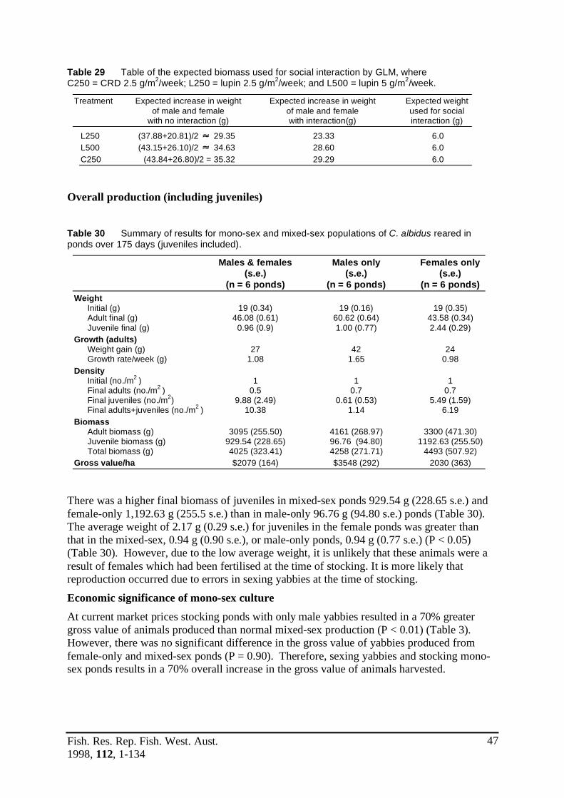
Fish. Res. Rep. Fish. West. Aust. 1998, 112, 1-134
47
Table 29 Table of the expected biomass used for social interaction by GLM, where C250 = CRD 2.5 g/m2/week; L250 = lupin 2.5 g/m2/week; and L500 = lupin 5 g/m2/week.
Treatment Expected increase in weight Expected increase in weight Expected weight of male and female of male and female used for social with no interaction (g) with interaction(g) interaction (g)
L250 (37.88+20.81)/2 ! 29.35 23.33 6.0 L500 (43.15+26.10)/2 ! 34.63 28.60 6.0 C250 (43.84+26.80)/2 = 35.32 29.29 6.0
Overall production (including juveniles) Table 30 Summary of results for mono-sex and mixed-sex populations of C. albidus reared in ponds over 175 days (juveniles included).
Males & females Males only Females only (s.e.) (s.e.) (s.e.) (n = 6 ponds) (n = 6 ponds) (n = 6 ponds) Weight
Initial (g) 19 (0.34) 19 (0.16) 19 (0.35) Adult final (g) 46.08 (0.61) 60.62 (0.64) 43.58 (0.34) Juvenile final (g) 0.96 (0.9) 1.00 (0.77) 2.44 (0.29)
Growth (adults) Weight gain (g) 27 42 24 Growth rate/week (g) 1.08 1.65 0.98
Density Initial (no./m2 ) 1 1 1 Final adults (no./m2 ) 0.5 0.7 0.7 Final juveniles (no./m2) 9.88 (2.49) 0.61 (0.53) 5.49 (1.59) Final adults+juveniles (no./m2 ) 10.38 1.14 6.19
Biomass Adult biomass (g) 3095 (255.50) 4161 (268.97) 3300 (471.30) Juvenile biomass (g) 929.54 (228.65) 96.76 (94.80) 1192.63 (255.50) Total biomass (g) 4025 (323.41) 4258 (271.71) 4493 (507.92)
Gross value/ha $2079 (164) $3548 (292) 2030 (363)
There was a higher final biomass of juveniles in mixed-sex ponds 929.54 g (228.65 s.e.) and female-only 1,192.63 g (255.5 s.e.) than in male-only 96.76 g (94.80 s.e.) ponds (Table 30). The average weight of 2.17 g (0.29 s.e.) for juveniles in the female ponds was greater than that in the mixed-sex, 0.94 g (0.90 s.e.), or male-only ponds, 0.94 g (0.77 s.e.) (P < 0.05) (Table 30). However, due to the low average weight, it is unlikely that these animals were a result of females which had been fertilised at the time of stocking. It is more likely that reproduction occurred due to errors in sexing yabbies at the time of stocking.
Economic significance of mono-sex culture At current market prices stocking ponds with only male yabbies resulted in a 70% greater gross value of animals produced than normal mixed-sex production (P < 0.01) (Table 3). However, there was no significant difference in the gross value of yabbies produced from female-only and mixed-sex ponds (P = 0.90). Therefore, sexing yabbies and stocking mono-sex ponds results in a 70% overall increase in the gross value of animals harvested.
Fish. Res. Rep. Fish. West. Aust. 1998, 112, 1-134
48
Discussion
Yabbies in a male mono-sex population grow faster than yabbies in either a female mono-sex population or in a mixed-sex (1:1) population. In this study the male mono-sex populations grew on average 68.36% faster than the female mono-sex animals and 52.77% faster than the mixed-sex population. Female yabbies in mono-sex culture grow 9.26% slower than those in mixed-sex populations, but this was not significant (P = 0.31).
The increased growth of male-only populations in comparison with the female-only populations may be attributable to sexual dimorphism, Woodland (1967) reported that male yabbies grow at the same rate as females until sexual maturity, after which female growth slows relative to that of males.
Both males and females in mono-sex cultures grew faster than males or females in a mixed-sex culture. Males in mono-sex culture grew 17% faster than males in mixed-sex populations; similarly, females in a mono-sex cultures grew 31% faster than those in mixed-sex populations.
The improved growth of both male and female mono-sex populations, relative to each sex in mixed-sex populations, may be due to the diversion of energy in mixed-sex populations from somatic growth to reproductive effort i.e. competition for mates and production of gametes. Alternatively, the observed increase in growth may be a result of limiting the production of juveniles and therefore density in the mono-sex treatments. There was no significant difference in the survival of either males or females in mono-sex culture compared with yabbies in mixed-sex culture. This experiment has shown that stocking ponds with only male yabbies results in a 70% greater gross value of animals produced than normal mixed-sex production. References
Akaike, H. 1974. A new look at the statistical model identification. IEEE Transactions on Automatic Control, 19(6): 716-721.
Cohen, D., Sagi, A., Ra’anan, Z. and Zohar, G. 1988. The production of Macrobrachium rosenbergii in mono-sex populations III: yield characteristics under intensive monoculture conditions in earthen ponds. Bamidgeh, 40: 57-63.
Curtis, M.C. and Jones, C.M. 1995. Observations on mono-sex culture of redclaw crayfish Cherax quadricarinatus von Martens (Decapoda: Parastacidae) in earthen ponds. J. World Aqua. Soc., 26(2): 154-159.
Faragher, R.A. 1983. Role of the crayfish Cherax destructor Clark as food for trout in Lake Eucumbene, New South Wales. Aust. J. Mar. Freshwater Res., 33: 407-417.
Lake, P.S. and Sokol, A. 1986. Ecology of the yabby Cherax destructor Clark (Crustacea : Decapoda : Parastacidae) and its potential as a sentinel animal for mercury and lead pollution. Australian Water Resources Council Technical Paper No. 87, 186p.
McClain, W.R., 1994. Investigations of crayfish density and supplemental feeding as factors influencing growth and production of Procambarus clarkii. In: Geddes, M.C., Fielder, D.R. and Richardson, A.M. / (eds.) Freshwater Crayfish X, Proceedings of the International Association of Astacology Tenth Symposium 1994, Adelaide, Australia, 10: 512-520.
McCullagh, P. and Nedler, J.A., 1986. Generalized Linear Models, 2nd ed, Chapman and Hall, London.

Fish. Res. Rep. Fish. West. Aust. 1998, 112, 1-134
49
Sagi, A., Ra’anan, Z., Cohen, D. and Wax, Y. 1986. Production of Macrobrachium rosenbergii in mono-sex populations: yield characteristics under intensive monoculture conditions in cages. Aquaculture, 51: 265-275.
Stearns, S.C. 1976. Life history tactics: A review of the ideas. Quart. Rev. Biol., 51(1): 3-45. Woodland, D.J. 1967. Population study of a freshwater crayfish Cherax albidus Clark: with
particular reference to the ecoenergetics of a population. PhD thesis, University of New England, Armidale, NSW, 283p.
D) Sediment oxidising agent 3.6 The use of calcium nitrate to increase dissolved oxygen levels Introduction
The farming of yabbies in Western Australia is based upon the use of existing undrainable ponds referred to as farm dams. This relatively new form of aquaculture is reliant upon natural food chains, low cost supplementary feeds and annual rainfall run-off into dams for water supply. Due to the use of existing farm dams, which have been constructed for the prime purpose of watering agricultural stock, design limitations necessitate the extensive (i.e. low stocking densities, low feed inputs) nature of this industry. It is impractical to drain these deep dams for aquaculture stock management to control populations, and it is uneconomic to connect power to farm dams for operating electric aerators. Consequently, the amount of supplementary feed that may be added without resulting in low dissolved oxygen due to biological oxygen demand (BOD) is limited. As a natural consequence of the annual cycle of inundation of dams, often incorporating substantial inputs of allochthanous (produced outside and brought into the dam) organic matter in run-off from pasture, and in addition to supplementary feeding, the bottom of the farm dams have high levels of dark anaerobic sediments and low dissolved oxygen levels. These conditions are not conducive to the rearing of aquatic species and limit the carrying capacity of the water body and therefore total production of bottom living freshwater crayfish species such as yabbies.
The addition of sodium nitrate has been proposed by Boyd (1995), Masuda and Boyd (1994) and Avnimelech and Zohar (1986) as a method for improving denitrification which is a process through which organic substances in sediments are oxidised with nitrate. Addition of nitrates to the pond may serve to oxidise anaerobic sediment pockets in the system. The advantage of nitrates over alternative oxidising agents is that nitrates operate as such only at redox potentials below 340 mV and thus will be activated only at anaerobic sites (Avnimelech and Zohar 1986). It is inappropriate to add sodium in the form of sodium nitrate to farm dams, which are already facing increasing salinity, for this experiment. Calcium nitrate was selected as a suitable substance for oxidising the anaerobic benthos while simultaneously releasing calcium available for uptake for shell formation during ecdysis by yabbies.

Fish. Res. Rep. Fish. West. Aust. 1998, 112, 1-134
50
Aim
The aim of this experiment was to record whether the addition of calcium nitrate to ponds could increase dissolved oxygen at the pond bottom and decrease the depth of the anaerobic sediments.
Research Station Experiment 3 Materials and methods
The effect of calcium nitrate upon the pond environment under four feeding regimes was investigated: lupins at 2.5 g/m2/week; lupins at 10 g/m2/week; crayfish reference diet at 10 g/m2/week; and meat at 10 g/m2/week. Each of these four feeding regimes (controls) was replicated three times. For each feeding regime, three ponds were fed in an identical manner with the addition of calcium nitrate. Calcium nitrate was added according to the rate described by Musada and Boyd (1994) for sodium nitrate, 50 g/L/week.
Each of the eight treatments, (four control diets and four control diets + calcium nitrate), were replicated three times in a randomised block design using 24 ponds each 100 m2. Ponds were stocked with yabbies at the rate of 1/m2. Initial mean stocking weight was 25.92 g (0.40 s.e.). The experimental ponds were stocked on 22 January 1996 and completed after 108 days on 8 May 1996. During the experiment, surface and bottom temperature (oC), and dissolved oxygen (mg/L) concentrations were recorded for each treatment using a YSI 55 dissolved oxygen meter. Water samples were obtained from each pond at the beginning, middle and end of the trial. Samples were submitted to the WA Chemistry Centre for analysis of calcium concentration (by ICP-AES), electrical conductivity (at 25°C by ion selective electrode method) and nitrogen-nitrate fraction (by copperised cadmium reduction method and colorimetric analysis of dye formation using a segmented flow auto analyser).
At the conclusion of the experiment sediment cores were taken from each pond using a corer with a clear perspex tube. From each pond three core samples each 20 cm deep were obtained. While in the clear perspex tube each core was measured to determine the depth from the sediment-water interface to the bottom of the aerobic sediment (brown), where the anaerobic sediment (black) layer commenced. An ORP Scan redox meter was used to measure redox potential at the water surface and bottom (sediment-water interface) at the conclusion of the experiment. Results
Dissolved oxygen Surface and bottom water temperature data demonstrated that the ponds were thermally stratified as would be expected for a farm dam or pond without mechanical aeration at this time of the year (Figure 16). Any increase in bottom dissolved oxygen levels in the thermally stratified ponds can therefore be attributed to the effect of calcium nitrate, rather than to mixing (as could occur in an unstratified water body).
The bottom dissolved oxygen data showed that dissolved oxygen concentrations at the benthos in ponds receiving calcium nitrate was higher than in untreated ponds for each of the diet treatments (Figure 16, Table 31). For each of the diet regimes, a t-test demonstrated a significant difference (P < 0.05) in bottom dissolved oxygen concentration between ponds

Fish. Res. Rep. Fish. West. Aust. 1998, 112, 1-134
51
with calcium nitrate treatment and those without, except for the crayfish reference diet (P = 0.06) regime.
0
5
10
15
20
25L2
.5
L2.5
+Cal
cium
nitra
te
L10
L10+
Cal
cium
nitra
te M10
M10
+Cal
cium
nitra
te
CR
D10
CR
D10
+Cal
cium
nitra
teTreatment
Tem
pera
ture
(0 C)
0
2
4
6
8
10
12
14
16
18
20
D.O
. (m
g/l)
SURFACE TEMPBOTTOM TEMPBOTTOM DO
Figure 16 Mean (± s.e.) surface and bottom water temperature and bottom dissolved oxygen (DO) for calcium nitrate treated Ca(N03)2 and untreated ponds for four feeding regimes: lupins 2.5 g/m2/week (L2.5); lupins 10 g/m2/week (L10); crayfish reference diet 10 g/m2/week (CRD10); and meat 10 g/m2/week (M10).
Table 31 Mean bottom dissolved oxygen levels (mg/L) in calcium nitrate treated and untreated ponds for four feeding regimes: lupins at 2.5 g/m2/week (L2.5); lupins at 10 g/m2/week (L10); crayfish reference diet at 10 g/m2/week (CRD10); and meat at 10 g/m2/week (M10).
Feeding regime Untreated (s.e.) Calcium nitrate (s.e.) L2.5 2.75 (0.11) 7.40 (1.03) L10 4.12 (0.28) 10.02 (0.75) M10 4.77 (0.77) 11.05 (0.77) CRD10 3.87 (1.26) 8.34 (1.97)
The addition of calcium nitrate increased both the surface and bottom dissolved oxygen concentrations for each of the treated pond-diet combinations (Figure 17). In addition the application of calcium nitrate decreased the difference between surface and bottom dissolved oxygen concentration.

Fish. Res. Rep. Fish. West. Aust. 1998, 112, 1-134
52
0
2
4
6
8
10
12
14
L2.5
L2.5
+Calc
iumni
trate
L10
L10+
Calci
umni
trate M
10
M10
+Calc
iumni
trate CR
D10
CRD1
0+Ca
lciu
m n
itrat
e
Treatment
D.O.
(mg/
l)
SURFACE DOBOTTOM DO
Figure 17 Mean (± s.e.) surface and bottom dissolved oxygen (DO) for calcium nitrate treated Ca(N03)2 and untreated ponds for four feeding regimes: lupins at 2.5 g/m2/week (L2.5); lupins at 10 g/m2/week (L10); crayfish reference diet at 10 g/m2/week (CRD10); and meat at 10 g/m2/week (M10).
Redox potential The redox potential of water in ponds treated with calcium nitrate was higher than for corresponding diet treatments without calcium nitrate additions (Figure 18). However, the difference between control and calcium nitrate treated ponds was not significant at the 0.05 level.
0
10
20
30
40
50
60
70
L2.5
L2.5
+Cal
ciu
m n
itrat
e L10
L10+
Cal
cium
nitra
te M10
M10
+Cal
ciu
m n
itrat
e
CR
D10
CR
D10
+Cal
cium
nitr
ate
Treatment
Redo
x (m
v)
Figure 18 Mean (± s.e.) water redox (mv) of calcium nitrate treated Ca(N03)2 and untreated ponds for four feeding regimes: lupins at 2.5 g/m2/week (L2.5); lupins at 10 g/m2/week (L10); crayfish reference diet at 10 g/m2/week (CRD10); and meat at 10 g/m2/week (M10).
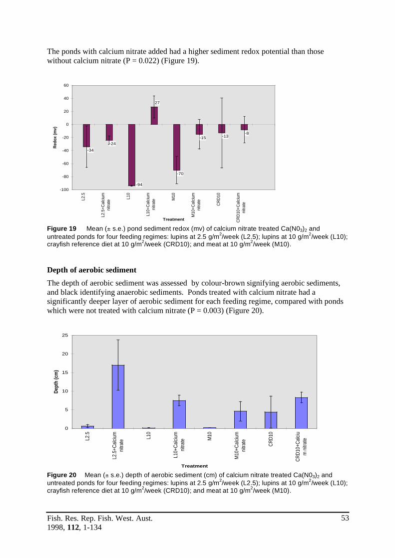
Fish. Res. Rep. Fish. West. Aust. 1998, 112, 1-134
53
The ponds with calcium nitrate added had a higher sediment redox potential than those without calcium nitrate (P = 0.022) (Figure 19).
-8-13-15
-70
27
-94
-24-34
-100
-80
-60
-40
-20
0
20
40
60L2
.5
L2.5
+Cal
cium
nitra
te
L10
L10+
Calci
umni
trate M
10
M10
+Cal
cium
nitra
te
CRD1
0
CRD1
0+Ca
lcium
nitra
te
Treatment
Redo
x (m
v)
Figure 19 Mean (± s.e.) pond sediment redox (mv) of calcium nitrate treated Ca(N03)2 and untreated ponds for four feeding regimes: lupins at 2.5 g/m2/week (L2.5); lupins at 10 g/m2/week (L10); crayfish reference diet at 10 g/m2/week (CRD10); and meat at 10 g/m2/week (M10).
Depth of aerobic sediment The depth of aerobic sediment was assessed by colour-brown signifying aerobic sediments, and black identifying anaerobic sediments. Ponds treated with calcium nitrate had a significantly deeper layer of aerobic sediment for each feeding regime, compared with ponds which were not treated with calcium nitrate (P = 0.003) (Figure 20).
0
5
10
15
20
25
L2.5
L2.5
+Calc
iumnit
rate
L10
L10+
Calci
umnit
rate M
10
M10
+Calc
iumnit
rate CR
D10
CRD1
0+Ca
lciu
m n
itrat
e
Treatment
Dept
h (c
m)
Figure 20 Mean (± s.e.) depth of aerobic sediment (cm) of calcium nitrate treated Ca(N03)2 and untreated ponds for four feeding regimes: lupins at 2.5 g/m2/week (L2.5); lupins at 10 g/m2/week (L10); crayfish reference diet at 10 g/m2/week (CRD10); and meat at 10 g/m2/week (M10).

Fish. Res. Rep. Fish. West. Aust. 1998, 112, 1-134
54
Although calcium nitrate improved the environmental conditions for yabby growth, there was no significant improvement in growth for either of the four feeding regimes: for lupins at 2.5 g/m2/week, P = 0.07; for lupins at 10 g/m2/week, P = 0.09; for the crayfish reference diet at 10 g/m2/week, P = 0.15; and for the meat at 10 g/m2/week, P = 0.57 (Table 32). Table 32 Growth of yabbies fed on three different diets with and without calcium nitrate.
Diet Mean weight increase (g) s.e. Lupins at 2.5 g/m2/week 18.69 2.48 Lupins at 2.5 g/m2/week + Ca(N03)2 11.68 1.57 Crayfish Reference Diet at 10 g/m2/week 29.26 1.10 Crayfish Reference Diet at 10 g/m2/week + Ca(N03)2 26.71 0.96 Lupins at 10 g/m2/week 23.81 2.10 Lupins at 10 g/m2/week + Ca(N03)2 18.48 1.31 Meat at 10 g/m2/week 18.91 2.17 Meat at 10 g/m2/week + Ca(N03)2 20.84 2.23
The reduced growth in the majority of the feeding regimes is thought to be due to the high levels of nitrate, as up to 97 mg/L was recorded in the ponds receiving calcium nitrate. While acceptable nitrate levels for yabbies are not known; for fish, levels below 1.0 mg/L are considered acceptable for continuous exposure and concentrations greater than 100 mg/L have been associated with fish kills (Langdon 1988). Discussion
The application of calcium nitrate to farm dam research ponds increased dissolved oxygen levels at both the surface and, in particular, the bottom sediment-water interface which yabbies inhabit.
The calcium nitrate prevented the build up of anaerobic waste from supplementary feeding, commonly observed in pond culture and farm dams in particular.
The application of calcium nitrate had therefore demonstrated potential for improving environmental conditions for aquaculture of crayfish in farm dams and ponds.
However, the rate of nitrate application used in this study gave very high nitrate levels and depths of aerobic sediments which indicated that reduced application rates may prove to be effective in farm dams and ponds. The effects of reduced rates of calcium nitrate on growth rate are currently being evaluated. References
Avnimelech, Y. and Zohar, G. 1986. The effect of local anaerobic conditions on growth retardation in aquaculture systems. Aquaculture, 58: 167-174.
Boyd, C.E. 1995. Potential of sodium nitrate to improve environmental conditions in aquaculture ponds. World Aquaculture, 26(2): 38-40.
Langdon, J.S. 1988. Investigation of fish kills. I: History and causes. In Bryden, D.I. (ed.) Fish diseases refresher course for veterinarians, Proceedings 106: 167-194.
Masuda, K. and Boyd, C.E. 1994. Effects of aeration, alum treatment, liming, and organic matter application on phosphorus exchange between soil and water in aquaculture ponds at Auburn, Alabama. J. World Aqua. Soc., 25(3): 405-416.

Fish. Res. Rep. Fish. West. Aust. 1998, 112, 1-134
55
E) Trap harvesting 3.7 Size and sex composition of yabbies in traps Introduction
Unlike most aquaculture ponds that can be drained to harvest animals, farm dams although subject to fluctuating water levels, usually retain some water throughout the year and are not designed to be drained. Furthermore, as the main purpose of farm dams is to water sheep during the annual period of summer drought, wasting water by draining is impracticable. Consequently, yabbies in Western Australian farm dams are harvested using baited traps. Aim
To record the effect of trapping on the yabby population. Materials and methods
At the conclusion of the first research station experiment, traps were placed in each of the six control ponds prior to emptying. Traps were placed at a density of one trap per 25 m2 and remained in the pond overnight. Total numbers of male and female yabbies collected from each trap were recorded. Immediately after removing traps, the ponds were drained. After draining, the total numbers of male and female yabbies collected from each pond were recorded. To satisfy the assumption of normality, the proportions of male and female yabbies trapped were transformed with the arcsine square root transformation, prior to using analysis of variance. Results
There was a significant difference in the percentage of males collected by trapping compared with draining (P < 0.001). Males are 2.7 times more likely to be caught by trapping (Table 33). There was no significant difference in the percentage of females collected by either trapping or draining (P = 0.34). Table 33 Percentage of males and females collected from ponds by trapping and draining (n = 410).
% Males % Males % Females % Females trapped drained trapped drained Mean 73 27 52 48 s.e. 4.91 4.91 3.31 3.31
Of the berried females in this experiment, 14% were removed from the ponds by trapping, while 86% remained in the ponds after trapping and were collected after draining the ponds. Therefore, berried females are either less likely to enter traps or are prevented from doing so by males already in the traps. Discussion
The harvesting method currently used by the farm dam yabby industry in Western Australia, selectively removes males while leaving females, in particular berried females, in farm dams. This trapping bias is likely to result in a skewed sex ratio which favours the slower growing, but high fecundity females.

Fish. Res. Rep. Fish. West. Aust. 1998, 112, 1-134
56
Repeated trapping of industry farm dams will magnify the results obtained here from a single trapping experiment. In addition, as industry harvesters remove the largest yabbies for market and throw back smaller animals “to grow more”, the large males are being removed from the farm dams, while smaller and possibly slower growing males (i.e. runts), along with females are thrown back to contribute to the gene pool.
It has been shown that yabbies grow slower at higher densities (section 3.2) and that male yabbies grow faster than female yabbies (section 3.5). Industry’s reports of high numbers of yabbies below market size (< 30 g) and dams becoming less productive over time, may be a result of trapping selectivity, which leaves berried females capable of producing large numbers of juveniles in farm dams with a resultant increase in density. The hypothesis that the sex ratio and size distribution of yabbies is skewed in industry farm dams by trapping is further investigated in section 4.2. Methods for managing this problem in the farm dam yabby population are currently being evaluated at the Avondale research station and, if successful, will be trialed in industry farm dams.
4.0 Industry farm dam recording system
A) Baseline survey - yabby size, sex ratio and the farm dam environment
4.1 The relationship between physical, chemical and biological parameters and yabby production in industry farm dams
Introduction
The harvesting of yabbies (Cherax albidus) from farms dams in Western Australia occurs over an area of approximately 750,000 km2 throughout the south-west inland Wheatbelt region (Figure 21).
Longitude (East)
Latit
ude
(Sou
th)
115 116 117 118 119 120
36
35
34
33
32
31
Perth
Albany
Enlarged region
DDD
DDDD
D DD
DDD
DDD
DD
DDD
A
Figure 21 Location of the 21 logbook dams (D) and the Avondale research station (A) in Western Australia.

Fish. Res. Rep. Fish. West. Aust. 1998, 112, 1-134
57
Farm dams were constructed for the prime purpose of watering sheep during the annual period of summer drought, not for rearing yabbies. Consequently, while water quality and environmental parameters are usually within the range acceptable for sheep, they are not necessarily ideal for the aquaculture of yabbies. Yabby farmers have reported considerable variation in yabby yields between farm dams and changes in production from individual dams over time (Table 34). However, it is not known whether this variation is due to regional physical, chemical and/or biological parameters (Morrissy 1980). The investigation of environmental parameters from industry farm dams, recorded here, was based upon information obtained from logbooks and research sampling. The study provided baseline industry data on physical, chemical and biological parameters of dams, stocks and harvesting practices. This study investigates the effect of physical and chemical factors upon yabby production from farm dams in WA. The four responses investigated were: Yield (g/m2/year); Density (yabbies/m2); Return ($/m2/year); and Return/Cost ($return/$cost). Yield was defined as the total weight of yabbies harvested as g/m2. Density (yabbies/m2) was determined by trawling each dam according to the methods described in section 4.2. Return was calculated by attributing standard industry values according to weight grades of yabbies trapped from each dam expressed as $/m2/week. Return/cost was calculated as value of yabbies harvested divided by value of feed fed and expressed as $return/$cost. Multiple regression was used to select the most important physical and chemical factors that would affect yabby production for these responses. Materials and methods
Data were collected on 21 farm dams used for commercial yabby harvesting (Figure 21). Dams were selected to represent the diverse range of conditions and feeding protocols observed in Western Australia. Each dam was assigned an identifying code number (D1,...,H3). Water samples were collected for water chemistry analyses twice, in December 1994 and June-August 1996. Samples were submitted to the Chemistry Centre of WA for analyses of: Alkalinity, total expressed as CaCO3
(mg/L); CO3 (Carbonate); Ca (Calcium); Cl (Chloride); Cu (Copper, total); Electrical conductivity (25°C); Fe (Iron); Fe-total (Iron, total); HCO3 (bicarbonate); Hardness, total expressed as CaCO3
(mg/L); K (Potassium); Mn (Manganese); Mn-total (Manganese, total); N-NO3 (Nitrogen, nitrate + nitrite fraction); Na (Sodium); P-SR (Phosphorous, soluble reactive); SO4-S (Sulphate, sulphur expressed as sulphate); TSS (Total soluble salts); Zn-total (Zinc, total); and pH.
Physical data were recorded on altitude of farm dam on catchment height (1 = low; 2 = medium; 3 = high), dam size (surface area, m2; volume, m3), clay colour (1 = red; 0 = white), rainfall (mm), Secchi disk depth (cm) (as an indicator of turbidity), wind exposure (average speed and direction in relationship to dam mouth), bank height (m), percentage of organic matter in sediments, age of dam (years), and latitude and longitude. Farmers were interviewed to record the past history of each dam, including the periods over which it had been harvested, feed type and the age of the dam in years. During the summer harvesting period of 1994-95, farmers filled in logbooks to record biological data on feeding and yield of yabbies from each dam. Yabbies from each trapping were graded according to numbers in each weight grade: < 20 g, 20-30 g, 30-40 g, 40-50 g, 50-70 g, 70-100 g and > 100 g. The type and quantity of food added between each trapping period were recorded by farmers.

Fish. Res. Rep. Fish. West. Aust. 1998, 112, 1-134
58
Multiple linear regression methods In most field biological research problems where regression analysis is applied, more than one predictor variable is needed in the regression model, therefore a multiple regression is needed. When this model is linear in the coefficients, it is called a multiple linear regression model. If the k predictor variable is x x xk1 2, ,..., , and the response variable is y, the multiple linear regression model is:
y x xk k= + + + +! ! ! "0 1 1 ...
and the estimated response is obtained from the sample regression equation:
$ $ $ ... $y x xk k= + + +! ! !0 1 1
Where ! "~ ( , )NID 0 2 and regression coefficients !i , i = 1,...,k, are estimated by $!i from the sample data using the method of least squares.
The dams in this study permitted 21 observations with 10 to 20 predicator variables, (although in some cases there were 2 to 4 predicator variables missing from the data). It was assumed there is no higher order interaction and the effect from each predictor variable is linear.
It is necessary to check whether there are outlier(s), collinearity between predictor variables, and that the residuals are independently normally distributed. Cook’s distance and residual plots were used to select possible outlier(s) in each sample multiple regression. Residual plots and quantile-normal quantile plots were used to check the various assumptions of the multiple regression models. Student’s t-test was used to test whether !i i k= =0 1 2, , ,..., or not. The criterion used to select the necessary parameters in the models was AIC (Akaike 1974) where:
AIC n RSS n p= +log( / ) 2 Where RSS is residual sum of square, n is the number of observations and p is number of parameters need to be estimated.
Results
There was a wide range in each of the response variables, yield, yield/harvest, return, return/cost, density and total annual return, for the 21 dams in the study (Table 34). This supports reports from industry that some dams are more productive. The most productive dams produced a yield of 34 g/m2/year of yabbies valued at over $2,000 per year.
Table 34 Summary statistics (minimum, maximum, median and mean) of the response variables for 21 farm dams.
Response Minimum Maximum Median Mean Yield (g/m2/week) 0.0058 0.67 0.11 0.19 Yield/year (g/m2/year) 0.31 34.82 10.23 5.77 Mean yield/harvest (g/m2/harvest) 0.0015 0.096 0.028 0.035 Return ($/m2/week) 0.0008 0.02 0.0058 0.0077 Return/cost ($return/$cost) 3.11 33.06 10.94 14.63 Density (yabbies/m2) 0.13 17.43 3.32 4.86 Total annual return ($) 61.07 2037 478.50 570.90
Chemical toxicities to fish species vary considerably (according to species, age, stress and environmental variables) and even though in many cases they are unknown for yabbies, the

Fish. Res. Rep. Fish. West. Aust. 1998, 112, 1-134
59
levels associated with fish kills and acceptable continuous exposure, provide a basis for evaluating water quality (Langdon 1988). The water chemistry analyses show that, on average, levels of zinc, nitrate, iron and copper in WA farm dams are above those recommended for continuous exposure (Table 35). Maximum levels of manganese are greater than those recommended for continuous exposure (Table 35). In addition, the maximum levels recorded for alkalinity, iron, hardness and zinc exceed those previously associated with fish kills (Table 35).
Table 35 Summary of water chemistry (mean, minimum and maximum) recorded during summer and winter from 21 WA farm dams currently harvested for yabbies (water quality criteria adapted from Langdon 1988; Train 1979; Hart 1974; Mills and Geddes 1980).
Parameter Unit Mean Min Max Levels Acceptable associated continuous with fish kills exposure levels Alkalinity mg/L 127 20 270 >200 20-200 Copper total mg/L 0.024 < 0.02 0.05 >0.03-0.07 (soft water) >0.6-6.4 (hard water) < 0.006 Salinity mg/L 323 120 690 25 000 < 12 000 Iron mg/L 0.56 0.05 7.10 >0.5 < 0.1 Hardness mg/L 82.43 16 270 >200 20-200 Manganese total mg/L 0.062 < 0.02 0.05 >75 < 0.01 Nitrate mg/L 1.85 0.02 16 >100 < 1.0 Zinc total mg/L 0.045 0.02 0.68 >0.4-1.76 < 0.005 pH 7.63 5.00 8.20 < 4-5, >9-10 6.7-8.6
While water chemistry parameters may not necessarily result in yabby mortalities, levels which exceed those recommended for continuous exposure may limit yabby growth and production (i.e. alkalinity, Copper, Iron, hardness, manganese, nitrate and zinc). In addition minimum parameters for alkalinity, CO3, Ca, Cl, conductivity, HCO3, hardness, Na and pH are considered to be very low.
Summaries of chemical factors in summer, chemical factors in winter and physical factors (Tables 36, 37 and 38) show that the mean of each chemical factor in summer and winter was similar.

Fish. Res. Rep. Fish. West. Aust. 1998, 112, 1-134
60
Table 36 Summary of chemical factors in summer with minimum, maximum, median and mean.
Predictor variable(s) Unit Min. Max. Median Mean Alkalinity mg/L 20.00 250.00 99.00 111.80 Calcium mg/L 2.00 32.00 11.00 13.00 Chloride mg/L 23.00 260.00 63.00 82.43 Econd mS/m 19.70 126.00 44.20 53.92 Iron mg/L 0.050 7.10 0.17 0.88 Iron total mg/L 2.00 250.00 14.00 34.01 Hydrogen Carbonate mg/L 33.00 300.00 120.00 139.10 Hardness mg/L 26.00 160.00 69.00 82.57 Potassium mg/L 5.00 27.00 11.00 13.00 Manganese total mg/L 0.020 0.18 0.030 0.051 Nitrate mg/L 0.02 16.00 1.30 2.30 Sodium mg/L 24.00 233.00 67.00 86.05 Phosphorous mg/L 0.01 1.40 0.07 0.16 Sulphate mg/L 6.00 54.00 19.00 21.00 Total soluble salts mg/L 120.00 690.00 270.00 323.00 Zinc total mg/L 0.020 0.18 0.03 0.045 pH 7.10 8.50 7.70 7.74
Table 37 Summary of chemical factors in winter with minimum, maximum, median and mean.
Predictor variable(s) Unit Min. Max. Median Mean Alkalinity mg/L 33.00 270.00 140.00 142.4 Calcium mg/L 2.00 35.00 11.00 13.38 Chloride mg/L 22.00 220.00 98.00 98.52 Copper total mg/L 0.020 0.050 0.020 0.024 Econd mS/m 20.90 112.00 64.10 58.51 Iron mg/L 0.050 1.00 0.18 0.24 Iron total mg/L 2.90 160.00 13.00 26.31 Hydrogen Carbonate mg/L 40.00 330.00 170.00 174.20 Hardness mg/L 29.00 170.00 65.00 82.29 Potassium mg/L 6.00 33.00 13.00 14.76 Manganese total mg/L 0.02 0.46 0.04 0.072 Nitrate mg/L 0.32 3.00 1.10 1.40 Sodium mg/L 20.00 220.00 89.00 87.81 Phosphorous mg/L 0.02 5.90 0.12 0.62 Sulphate mg/L 4.00 59.00 19.00 21.62 Total soluble salts mg/L 120.00 620.00 350.00 322.90 Zinc total mg/L 0.02 0.13 0.030 0.044 pH 5.00 8.20 7.80 7.51

Fish. Res. Rep. Fish. West. Aust. 1998, 112, 1-134
61
Table 38 Summary of physical factors with minimum, maximum, median and mean.
PHYSICAL RESPONSES FACTORS Unit Min. Max. Median Mean Mean feed g/m2/week 0.017 3.38 0.31 0.61
rate Farmer opinion 0 = bad; 0.0 2.0 1.0 0.6
1 = good; 2 = very good
Age of dam years 0.13 17.43 5.10 7.01 Clay colour red = 1, 0.00 1.00 0.50 0.43
white = 0 Catchment 1 = low; 0.00 3.00 2.00 1.73
height 2 = medium; 3 = high
Harvests no./year 4.86 12.49 6.84 7.91 per year
Dam size m2 583 4039 1173 1477 Total feed kg/year 28.27 1847 145.10 305.20 Bank height m 0.50 4.00 1.00 1.55 Wind factor bank height x wind 0.17 4.08 0.60 1.37
direction/wind speed Wind speed m/sec 1.75 5.99 2.64 3.23 Wind 1 = front; 1.0 3.0 2.0 2.05
direction 2 = side; 3 = back
Latitude deg. min. 30.43 33.87 33.02 32.56 Longitude deg. min. 115.5 119.2 117.6 117.6 Rainfall mm 316.7 624.7 443.0 450.9 Secchi depth cm 2.50 28.00 7.50 9.33

Fish. Res. Rep. Fish. West. Aust. 1998, 112, 1-134
62
A matrix of correlation (r) between the responses (yield, return, return/cost and density) with water chemistry variables was constructed to show relationships. Most values for r were close to zero, with a range from-0.50 to 0.51, which indicates that no single water chemistry variable recorded has a strong relationship with yield, return, return/cost or density (Table 39).
Table 39 Matrix of correlations (r) between chemical parameters, yield, return and density for summer and winter water samples from farm dams.
CHEMICAL SUMMER WINTER PARAMETERS Yield Return Return/cost Density Yield Return Return/cost Density
Alkalinity 0.0026 -0.003 -0.15 -0.11 0.39 0.21 0.15 0.25 Calcium 0.10 0.18 -0.047 -0.22 0.34 0.27 0.31 0.0078 Chloride -0.18 0.16 0.18 -0.012 0.13 0.18 0.37 0.20 Copper total nil nil nil nil -0.27 -0.037 -0.10 0.20 ECond -0.099 0.14 0.090 -0.063 0.19 0.25 0.35 0.20 Iron -0.18 -0.18 -0.19 -0.13 0.21 -0.016 0.24 -0.071 Iron total -0.23 -0.23 -0.17 -0.098 -0.29 -0.19 -0.22 -0.11 Hydrogen -0.063 -0.073 -0.18 -0.17 0.39 0.21 0.16 0.24
Carbonate Hardness -0.13 0.085 -0.10 -0.32 0.34 0.41 0.40 0.18 Potassium 0.013 0.16 0.25 -0.22 0.21 0.24 0.51 -0.046 Manganese total -0.20 -0.28 0.059 -0.18 -0.26 -0.26 0.12 -0.028 Nitrate -0.19 0.016 0.047 -0.091 0.37 0.36 -0.16 0.13 Sodium -0.25 -0.15 0.024 -0.14 0.17 0.15 0.27 0.23 Phosphorus -0.12 0.060 0.042 -0.21 -0.25 -0.26 -0.095 -0.29 Sulphate -0.10 -0.007 0.22 -0.22 0.20 0.29 0.40 -0.15 Total soluble -0.27 -0.080 0.014 -0.22 0.20 0.25 0.35 0.20
salts Zinc total -0.33 -0.35 -0.20 -0.13 -0.43 -0.50 -0.31 -0.068 pH -0.21 -0.42 -0.039 -0.094 0.20 0.21 0.34 0.21
For density, all r values in summer were negative (Table 39). This indicates that the chemical variables which contribute to the water quality in farm dams during summer have a limiting effect upon yabby survival. In addition, it is highly likely that there are other chemical factors which have an important role in affecting the yabby production and/or the concentration of the chemical factors recorded was not low or high enough to affect yabby yields, return or return/cost. A matrix of correlation (r) between physical parameters, yield, return, return/cost and density varies from-0.43 to 0.998 (Table 40). Age of dam and density had a high correlation (r = 0.998), and therefore a good prediction of yabby density based upon a simple equation with the predictor variable Age of dam would be expected. There were strong relationships between Mean feed rate with Yield and Return.
In summer the correlation of alkalinity and hydrogen carbonate was 0.96; Chloride and electrical conductivity was 0.91; Chloride and Sodium was 0.7; Calcium and hardness was 0.72; Sodium and Chloride was 0.69; and Iron and Iron total was 0.95. Multiple linear regression used Electrical conductivity, Sodium (instead of Chloride), and Iron (instead of Iron total). Both Calcium and hardness were kept.

Fish. Res. Rep. Fish. West. Aust. 1998, 112, 1-134
63
Table 40 Matrix of correlations (r) between physical parameters, yield, return and density from farm dams.
PHYSICAL FACTORS RESPONSES Yield Return Return/cost Density Mean feed rate (g/m2/week) 0.76 0.67 -0.36 0.28 Farmer opinion 0.076 0.22 0.26 0.13
(0 = bad; 1 = good; 2 = very good) Age of dam (years) 0.38 0.28 -0.10 0.998 Density (yabby/m2) 0.30 0.22 -0.16 0.80 Clay colour -0.1 0.33 0.36 0.29
(red = 1; white = 0) Catchment height -0.59 -0.43 -0.18 -0.046
(1 = low; 2 = medium; 3 = high) Harvests per year 0.12 0.19 0.42 -0.11 Dam size (m2) -0.20 -0.11 0.050 0.044 Total feed (g/week) 0.55 0.69 -0.27 0.41 Bank height (m) 0.31 -0.022 -0.0043 0.38 Wind speed (m/sec) -0.26 -0.32 0.15 -0.36 Wind direction 0.41 -0.045 -0.0034 -0.073
(1 = front; 2 = side; 3 = back) Latitude (deg. min.) 0.36 0.32 -0.038 0.20 Longitude (deg. min.) -0.019 -0.036 -0.045 0.22 Rainfall (mm) 0.49 0.33 0.19 0.13 Secchi disk depth (cm) -0.027 0.0230 0.30 0.27
Some of the chemical factors for both winter and summer had a high correlation. To avoid collinearity between predictor variables. The cut-out point of |0.85| was used to select water chemistry variables for multiple linear regression in both summer and winter.
In summer the correlation of: Alkalinity and Hydrogen carbonate was 0.96; Chloride and electrical conductivity was 0.91; Chloride and Sodium was 0.7; Calcium and hardness was 0.72; Sodium and Chloride was 0.69; and Iron and Iron total was 0.95.
For multiple linear regression we used electrical conductivity, Sodium (instead of Chloride) and Iron (instead of Iron total). Both Calcium and hardness were kept. In winter the correlation of:
Electrical conductivity and total soluble salts was 1.0; Alkalinity and Hydrogen carbonate was 1.0; Sodium and Chloride was 0.89; Chloride and electrical conductivity was 0.91; Calcium and hardness was 0.89; Electrical conductivity and Sodium was 0.93; and Sodium and total soluble salts was 0.93.
Electrical conductivity (instead of total soluble salts, Sodium or Chloride); Calcium (instead of hardness); and alkalinity instead of Hydrogen carbonate were kept. There was also a high correlation between a number of physical factors. The correlation of wind factor and bank height was 0.86. Bank Height was kept because wind factor was

Fish. Res. Rep. Fish. West. Aust. 1998, 112, 1-134
64
dependent on bank height. The correlation of wind speed and latitude was-0.86. Both were kept because we expected they were independent predictor variables. Multiple linear regression results Multiple linear regression analyses were completed to determine how the responses yield (g/m2/week), return ($/m2/week), return/cost ($) and density (yabbies /m2) relate with the physical and chemical factors in the farm dams. Multiple linear regression analyses were completed for the significant coefficients of predictor variables for each of the four response variables for chemical factors in both summer and winter and for the physical factors. Using multiple linear regression, it is assumed that each predictor variable is approximately normally distributed and the product of the mean of each predictor variable and its estimated coefficient can be used to weight how important that predictor variable is in relation to the response. The results of multiple linear regression for important chemical factors in summer are listed in Tables 41, 42, 43 and 44; chemical factors in winter are listed in Tables 45, 46, 47 and 48; and physical factors are listed in Tables 49, 50, 51 and 52. A summary of all the factors with positive (+) and negative effects (-) are listed in Table 53. Table 41 Multiple linear regression results with “yield” as the response and water chemistry in summer as predictor variables. Where R2 = 0.17 and residual standard error = 0.1752 (d.f. = 17).
Predictor Mean Estimated P = Pr(>|t|) variable(s) coefficient( $!i )
Intercept - 0.18 0.08 Calcium 13.00 0.016 0.08 Hardness 82.57 -0.0022 0.14
Table 42 Multiple linear regression results with “return” as the response and water chemistry in summer as predictor variables. Where R2 = 0.38 and residual standard error = 0.004343 (d.f. = 17).
Predictor Mean Estimated P = Pr(>|t|) variable(s) coefficient( $!i )
Intercept - 0.0050 0.00 Nitrate 2.30 0.0019 0.00
Table 43 Multiple linear regression results with “return/cost” as the response and water chemistry in summer as predictor variables. Where R2 = 0.83 and residual standard error = 7.333 (d.f. = 17).
Predictor Mean Estimated P = Pr(>|t|) variable(s) coefficient( $!i )
Hardness 82.57 -0.12 0.04 Potassium 13.00 1.11 0.00 Sulphate 21.00 0.40 0.00

Fish. Res. Rep. Fish. West. Aust. 1998, 112, 1-134
65
Table 44 Multiple linear regression results with “density” as the response and water chemistry in summer as predictor variables. Where R2 = 0 and residual standard error = 5.036 (d.f. = 20).
Predictor Mean Estimated P = Pr(>|t|) variable(s) coefficient( $!i )
Intercept 4.86 0.00
Table 45 Multiple linear regression results with “yield” as the response and water chemistry in winter as predictor variables. Where R2 = 0.83 and residual standard error = 0.1177 (d.f. = 17).
Predictor Mean Estimated P = Pr(>|t|) variable(s) coefficient( $!i )
Alkalinity 142.4 0.0010 0.00 Copper total 0.024 -9.75 0.00 Iron 0.24 0.23 0.07 Nitrate 1.40 0.15 0.00
Table 46 Multiple linear regression results with “return” as the response and water chemistry in winter as predictor variables. Where R2 = 0.47 and residual standard error = 0.003615 (d.f. = 17).
Predictor Mean Estimated P = Pr(>|t|) variable(s) coefficient( $!i )
Intercept 0.0079 0.00 Nitrate 1.40 0.0024 0.03 Zinc total 0.044 -0.092 0.00
Table 47 Multiple linear regression results with “return/cost” as the response and water chemistry in winter as predictor variables. Where R2 = 0.83 and residual standard error = 7.733 (d.f. = 18).
Predictor Mean Estimated P = Pr(>|t|) variable(s) coefficient ( $!i )
Potassium 14.76 0.71 0.00 Sulphate 21.62 0.23 0.04
Table 48 Multiple linear regression results with “density” as the response and water chemistry in winter as predictor variables. Where R2 = 0 and residual standard error = 4.429 (d.f. = 18).
Predictor Mean Estimated P = Pr(>|t|) variable(s) coefficient( $!i )
Intercept 4.42 0.00
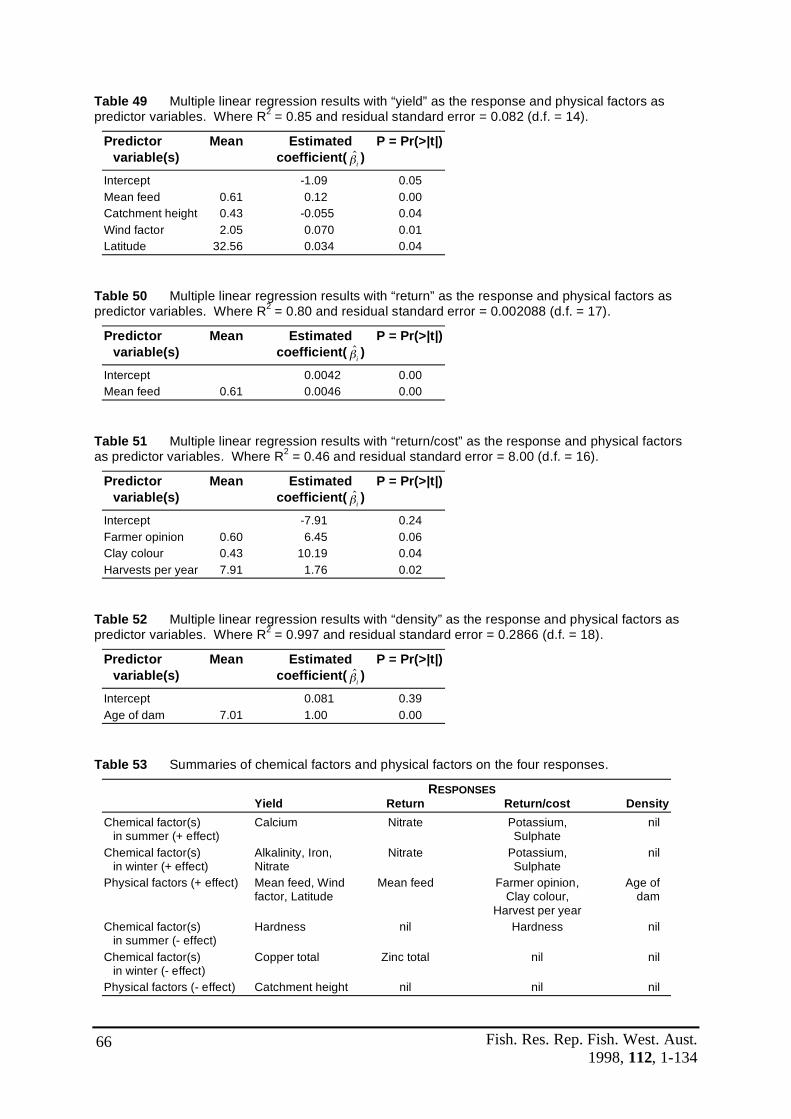
Fish. Res. Rep. Fish. West. Aust. 1998, 112, 1-134
66
Table 49 Multiple linear regression results with “yield” as the response and physical factors as predictor variables. Where R2 = 0.85 and residual standard error = 0.082 (d.f. = 14).
Predictor Mean Estimated P = Pr(>|t|) variable(s) coefficient( $!i )
Intercept -1.09 0.05 Mean feed 0.61 0.12 0.00 Catchment height 0.43 -0.055 0.04 Wind factor 2.05 0.070 0.01 Latitude 32.56 0.034 0.04
Table 50 Multiple linear regression results with “return” as the response and physical factors as predictor variables. Where R2 = 0.80 and residual standard error = 0.002088 (d.f. = 17).
Predictor Mean Estimated P = Pr(>|t|) variable(s) coefficient( $!i )
Intercept 0.0042 0.00 Mean feed 0.61 0.0046 0.00
Table 51 Multiple linear regression results with “return/cost” as the response and physical factors as predictor variables. Where R2 = 0.46 and residual standard error = 8.00 (d.f. = 16).
Predictor Mean Estimated P = Pr(>|t|) variable(s) coefficient( $!i )
Intercept -7.91 0.24 Farmer opinion 0.60 6.45 0.06 Clay colour 0.43 10.19 0.04 Harvests per year 7.91 1.76 0.02
Table 52 Multiple linear regression results with “density” as the response and physical factors as predictor variables. Where R2 = 0.997 and residual standard error = 0.2866 (d.f. = 18).
Predictor Mean Estimated P = Pr(>|t|) variable(s) coefficient( $!i )
Intercept 0.081 0.39 Age of dam 7.01 1.00 0.00
Table 53 Summaries of chemical factors and physical factors on the four responses.
RESPONSES Yield Return Return/cost Density Chemical factor(s) Calcium Nitrate Potassium, nil
in summer (+ effect) Sulphate Chemical factor(s) Alkalinity, Iron, Nitrate Potassium, nil
in winter (+ effect) Nitrate Sulphate Physical factors (+ effect) Mean feed, Wind Mean feed Farmer opinion, Age of
factor, Latitude Clay colour, dam Harvest per year
Chemical factor(s) Hardness nil Hardness nil in summer (- effect)
Chemical factor(s) Copper total Zinc total nil nil in winter (- effect)
Physical factors (- effect) Catchment height nil nil nil

Fish. Res. Rep. Fish. West. Aust. 1998, 112, 1-134
67
The R2 for chemical factors varied from 0 to 0.83 (Tables 41-48). As the R2 in Tables 43 and 45 both fitted with intercept equal to zero they could not properly explain for the random errors from the responses. Therefore, R2 should be from 0 to 0.47, this could be explained by the low correlation (r) between responses and predictor variables in Table 39. Chemical factors in both summer and winter did not have any effects on the density of yabbies in dams. Density of yabbies was 4.86 yabbies/m2 in summer. Nitrate in summer and winter had a positive effect on yield and return and is likely to be an indicator of productivity and therefore food resources in the farm dam environment. During summer, when yabbies grow and moult, calcium played a very important part in the water chemistry. As calcium is required for moulting and therefore growth of yabbies, this chemical parameter may limit production if it is not readily available.
Potassium and sulphate related with the return/cost and therefore contributed to production of larger yabbies, as the price received is directly related to the size of yabbies harvested. The reason for this is still unknown. Copper total, zinc and hardness had a negative impact on yabby production. These three chemical parameters were all recorded at levels above those recommended for continuous exposure (Table 35).
In the four tables of physical factors, R2 varied from 0.46 to 1.00 (Tables 49-52). This could be explained by the correlation (r) between the responses and predictor variables in Table 40. Mean feed rate was the most important variable positively effecting both yield and return. Mean feed rate could increase the yield with a slope equal to 0.0046, which was higher than the intercept 0.0042 (without feed) (Table 50). Wind direction had a positive effect on yield, most likely due to improved aeration and destratification due to wind mixing in those dams which faced the prevailing winds. Red clay was better than white clay for yabby production, the reason for this is unknown although the suggestion that red clay possesses a greater mineral content warrants investigation. Latitude had a positive effect on yield, with dams in southern regions producing more yabbies. This may be due to temperature or rainfall, or as a result of replicating environmental conditions similar to those of Victoria from where yabbies were translocated to WA.
The return on investment (return/cost) increased with the number of harvests per year. Farmer opinion was also very important and indicated that farmers can identify high producing dams based on past experience and trap yields. Dams which were low on the catchment were more productive than dams which were high on the catchment. This supports the farm dam production-eutrophication model, with dams low on the catchment receiving higher levels of allochthanous material, resulting in an increase in production due to increased food resources. The density of yabbies in dams was only affected by the age of dams. Older dams had higher densities of yabbies. As growth of yabbies is density dependent (section 3.2) this is likely to result in large numbers of small animals and may be due to selection pressure by trapping and/or inbreeding leading to stunted populations.
Fish. Res. Rep. Fish. West. Aust. 1998, 112, 1-134
68
Discussion
Compared with chemical factors, physical factors played a more important role in determining the yield, cost, return/cost and density. The main parameters limiting production in WA farm dams were feed and physical factors.
Limiting factors: i) Feed
Low feeding rates, high on catchment (reduced run-off) and low latitude (i.e. lower rainfall and/or less run-off) appear to limit food resources.
ii) Physical factors a) Aeration/stratification
Low wind exposure, low prevailing wind speed and high bank height (i.e. reduces the mixing effect of prevailing winds) reduce farm dam aeration;
b) Production area Small sized farm dams do not produce as many yabbies/dam, due to the obvious size constraint; high densities in dams reduce yabby production.
The high degree of variation between farm dams in this study has supported the hypothesis that some farm dams are more productive than others. Water chemistry parameters, while unlikely to be responsible for fish kills, were recorded at levels which may limit yabby production. Relationships between some of these factors and yield have been demonstrated (i.e. zinc, copper, hardness). The chemical factors investigated, however, have not indicated a very strong relationship between yield, return, return/cost and density, and therefore it is unlikely that any single chemical factor recorded in this study is the major factor limiting yabby production in WA farm dams. Linear or nonlinear regression gave values of R2 from 0.1 to 0.4 (except one with 0.6). With the omission of some outliers, the value of R2 varied from 0.1 to 0.5. This indicates that in order to predict the response with higher precision, it is necessary to obtain more predictor variables for each response. Alternatively higher order interactions may exist between the water chemistry predictor variables. Additional samples are required for estimation of higher order interaction between predictor variables.
The results obtained indicate that factors which may be limiting yabby production in WA farm dams are likely to be related to the "dam eutrophication-crayfish production continuum" model which previous work developed as the most promising basis for explaining the highly variable farm dam environment in WA (Morrissy 1980).
Current harvesting practices appear to have a negative affect upon yield of yabbies harvested and value of harvests. This may be a result of changes to the water chemistry or, alternatively, due to changes in population structure of yabbies as a result of harvesting. References
Akaike, H. 1974. A new look at statistical model identification. IEEE Transactions on Automatic Control, AU-19: 716-722.
Draper, N. and Smith, H. 1981. Applied Regression Analysis. John Wiley and Son.
Hart, B. 1974. A compilation of Australian water quality criteria. Australian Water Resources Council Technical Paper No. 7, 349p.
Langdon, J.S. 1988. Investigation of fish kills. I. History and causes. In Bryden, D.I. (ed.) Fish diseases refresher course for veterinarians. Proceedings 106: 167-194.

Fish. Res. Rep. Fish. West. Aust. 1998, 112, 1-134
69
Merrick, J.R. and Lambert, C.N. 1991. The Yabby, Marron and Red Claw Production and Marketing. JR Merrick Productions, Artarmon, NSW.
Mills, B.J. 1983. Aquaculture of yabbies. Proceedings of the first Freshwater Aquaculture Workshop. Dept. of Agriculture, NSW, pp. 89-98.
Mills, B.J. and Geddes, M.C. 1980. Salinity tolerance and osmoregulation of the Australian freshwater crayfish Cherax destructor Clark (Decapoda: Parastacidae). Aust. J. Mar. Freshwater Res., 31: 667-676.
Morrissy, N.M. 1980. Production of marron in Western Australian farm dams. Fish. Res. Bull. West. Aust., 24: 1-80.
Morrissy, N.M. & Cassells, G. 1992. Spread of the introduced yabby Cherax albidus Clark, 1936 in Western Australia. Fisheries Research Report (Fisheries WA), 92, 27p.
Morrissy, N.M. Evans, L. and Huner, J.V. 1990. Australian freshwater crayfish: Aquaculture species. World Aquaculture, 21(2): 113-122.
Train, R.E. 1979. Quality criteria for water. Castle House Publications Ltd. 256p.
4.2 Size distribution and sex ratio of yabbies from industry harvested dams Introduction
Many farmers report that the majority of yabbies in their farm dams are below market size (< 30 g). Many commercial growers attribute the large numbers of small yabbies in dams to under-feeding. In contrast, new dams which have not previously been trapped or fed, often yield exceptionally large yabbies. Therefore, it is hypothesised that harvesting farm dams by trapping may have a negative effect upon the yabby population structure. The catch composition of yabbies from trapping known populations at Avondale research station (section 3.7), showed that trapping selectively removes males in preference to females. Therefore, it is likely that with continued trapping the sex ratio of yabbies in farm dams would be skewed in favour of females. Furthermore, berried females are less likely to enter traps and are regarded as seconds, so when they are caught in traps, industry generally returns them to the dam. As industry generally remove the largest yabbies for market and throw back smaller animals “to grow more”, it is probable that large males are being removed from the farm dams, while slower growing males (runts) and females are thrown back to contribute to the gene pool. Aim
To determine the sex ratio of yabbies in farm dams being harvested by industry. Materials and methods
Twenty-seven farm dams which were being harvested using baited traps, were trawled by research staff between 18 June 1996 and 27 August 1996 to obtain the sex ratio and size distribution of yabbies.
Trawling gives an unbiased sex and size sample of the farm dam yabby population. However, it is destructive as it can result in damage to limbs and therefore trawling is not suitable for commercial harvesting. The trawl net, 3.6 m long and 2 m wide with a 5 mm mesh size, was dragged along the bottom across the diameter of each dam three times.

Fish. Res. Rep. Fish. West. Aust. 1998, 112, 1-134
70
Yabbies collected from trawls were graded and sexed. Results
While the sex ratio of yabbies was approximately equal in the lower size grades, in all of the larger size grades there were more females than males (Figure 22).
0
10
20
30
40
50
60
70
80
5-10 10-20 20-30 30-40 40-50 >50
Weight grade(g)
% c
ompo
sitio
n of
tot
al c
atch
Male
Female
Figure 22 Percentage composition of male and female yabbies by weight grade.
There was no significant difference in the percentage of males and females for the size grades 5-10 g, 10-20 g and over 50 g (Table 54). However, the proportion of females was significantly greater than males in the size grades 20-30 g, 40-50 g and 50-60 g (Table 54).
In total, across all size grades, there were more females than males in the 27 farm dams sampled, with an average sex ratio of 1 male to 1.2 females (Table 54).
Table 54 Size distribution according to weight grade and sex ratios of yabbies from 27 farm dams. Where n.s. = P > 0.5; * = P < 0.05; ** = P < 0.01; and *** = P < 0.001.
Weight No. No. Total Male Female P Statistical grade (G) male female (%) (%) significance 5-10 828 866 1694 49 51 0.82 n.s. 10-20 819 853 1672 49 51 0.08 n.s. 20-30 298 385 683 44 56 0.01 ** 30-40 111 253 364 30 70 0.0004 *** 40-50 68 145 213 32 68 0.005 ** >50 58 80 138 42 58 0.67 n.s. SUM 2181 2582 4763

Fish. Res. Rep. Fish. West. Aust. 1998, 112, 1-134
71
Discussion
The results obtained from this experiment are the opposite to what would be expected from the results of section 3.5 which demonstrated that male yabbies grow faster than females. Hence, it would be expected that in a natural water body, males would dominate the higher size grades, while females would be more prevalent in the lower size grades. It is possible that male yabbies, which have been shown to grow faster (section 3.5), have a higher rate of mortality, due to increased moulting. Recently moulted, soft yabbies are at a greater risk of cannibalism than inter-moult yabbies with hard shells.
However, it has been shown that traps used by industry to harvest yabbies from farm dams selectively remove more male than female yabbies (section 3.7).
Consequently, these results based upon a survey of 27 farm dams which are harvested by industry using traps, indicate that male yabbies in the larger size grades are being removed or more of them are dying, leaving the less easily trapped females in the dam. This hypothesis is supported by the data which demonstrate that the sex ratio of yabbies below market size is approximately 1:1, however, above market size the proportion of males compared with females is lower in all size categories.
These data support the hypothesis proposed in section 3.7 that reports of high numbers of yabbies below market size (< 30 g) and dams becoming less productive over time, may be a result of negative genetic selection due to trapping; as trapping removes the larger, faster growing males, while leaving berried females capable of producing large numbers of juveniles, with a resultant increase in density. The implications of this harvesting practice upon the density of yabbies, along with developing techniques for managing the sex composition of animals within farm dams, is being investigated in the current project.
B) Application of feeding experiment results in farm dams 4.3 The effect of feeding upon the production of yabbies in farm dams Introduction
Harvesting of yabbies from farm dams in Western Australia is based upon supplementary feeding of low cost, readily available lupins. At the commencement of this study in 1994, farmers and processors were interviewed to determine the average feeding regime for industry farm dams in Western Australia. The average feeding regime was reputedly lupins at the rate of 2.5 g/m2/week. Experiments at the Avondale research station showed that while a significant proportion of yabby growth could be attributed to natural food production, lupins provided increased yabby growth. However, increased feeding rates of lupins and more complete diets could provide further improvements in yabby growth (sections 3.3 and 3.4). Within the farm dam environment, which does not have water exchange or aeration, feeding rates will be limited to low levels to avoid deoxygenation due to eutrophication.

Fish. Res. Rep. Fish. West. Aust. 1998, 112, 1-134
72
Aims
1. To quantify the effect of feeding lupins in industry farm dams; and
2. To determine if feeds shown to provide increased growth at the research station can increase yabby production in poor yabby producing dams.
Materials and methods
Baseline data were collected on 27 farm dams being used for commercial yabby harvesting in December 1994. Each dam was assigned an identifying code number. Data were collected on dam size, feed type and feed quantities. During the summer harvesting period of 1994-95, farmers filled in logbooks to record management practices and yield of yabbies from each trapping harvest. Yabbies from each trapping were graded according to numbers in each weight grade of less than 20 g, 20-30 g, 30-40 g, 40-50 g, 50-70 g, 70-100 g and >100 g. The type and quantity of food added between each trapping period were recorded by farmers.
During the summer of 1995-96, the feed type which had shown the best growth in the research station experiments (CRD) was provided to six farm dams, at the rate of 2 g/m2/week to one dam (a conservative rate), 2.5 g/m2/week to four dams and 5 g/m2/week to the remaining dam. While feed was supplied in marked containers, the feed rates applied by farmers were considerably lower than had been previously planned in this experiment. Actual feed rates by farmers for CRD fed dams ranged from 0.5-3.38 g/m2/week.
The dams which were selected for feeding were those considered by farmers to be poorer producing in quality and quantity of yabbies. The remaining farm dams on each property retained the same feed and rate as the previous year to permit relative changes in yabby production to be recorded. Logbooks were completed by farmers to record information as in the previous year. Density and size distribution of yabbies in dams were assessed by research trawling of dams according to the methods previously presented in section 4.2. Results
Baseline survey of yabby production and feeding in farm dams During the study, feed rates for lupins ranged from 0.02 to 3.38 g/m2/week. The average feed rate for dams in this study was 0.59 g/m2/week. In general farmers were actually feeding a lower quantity of lupins than they had originally thought. The average feeding rate of dams in this experiment of 0.59 g/m2/week is considerably below the average feed rate of the industry (2.5 g/m2/week). The dams in this study, however, were chosen to represent a diverse range of conditions (region, location of paddock, perceived level of production) and hence were not a random sample. In particular, poor producing dams were sought in order to investigate factors causing lower production and methods for enhancing production. There was a high positive relationship (r = 0.84) between the feeding rate of lupins and yield of yabbies from farm dams (Figure 23). The dam with the highest mean weekly yield (G2) produced 0.67 g of yabbies/m2/week, with a feed rate of 3.38 g/m2/week.
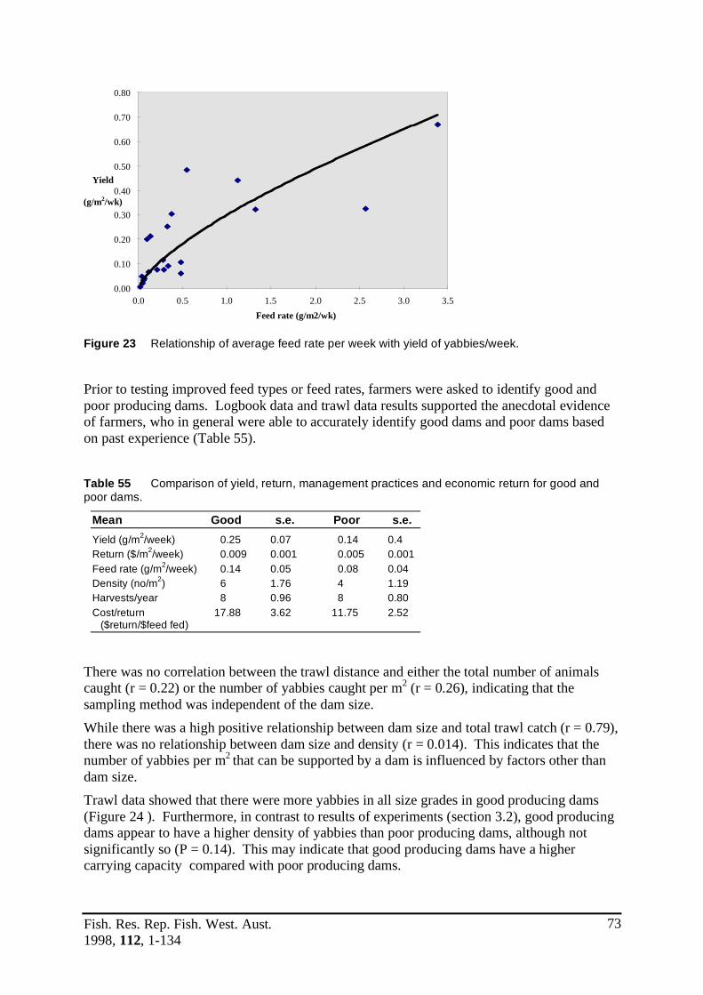
Fish. Res. Rep. Fish. West. Aust. 1998, 112, 1-134
73
0.00
0.10
0.20
0.30
0.40
0.50
0.60
0.70
0.80
0.0 0.5 1.0 1.5 2.0 2.5 3.0 3.5Feed rate (g/m2/wk)
Yield
(g/m2/wk)
Figure 23 Relationship of average feed rate per week with yield of yabbies/week.
Prior to testing improved feed types or feed rates, farmers were asked to identify good and poor producing dams. Logbook data and trawl data results supported the anecdotal evidence of farmers, who in general were able to accurately identify good dams and poor dams based on past experience (Table 55). Table 55 Comparison of yield, return, management practices and economic return for good and poor dams.
Mean Good s.e. Poor s.e. Yield (g/m2/week) 0.25 0.07 0.14 0.4 Return ($/m2/week) 0.009 0.001 0.005 0.001 Feed rate (g/m2/week) 0.14 0.05 0.08 0.04 Density (no/m2) 6 1.76 4 1.19 Harvests/year 8 0.96 8 0.80 Cost/return 17.88 3.62 11.75 2.52
($return/$feed fed)
There was no correlation between the trawl distance and either the total number of animals caught (r = 0.22) or the number of yabbies caught per m2 (r = 0.26), indicating that the sampling method was independent of the dam size. While there was a high positive relationship between dam size and total trawl catch (r = 0.79), there was no relationship between dam size and density (r = 0.014). This indicates that the number of yabbies per m2 that can be supported by a dam is influenced by factors other than dam size. Trawl data showed that there were more yabbies in all size grades in good producing dams (Figure 24 ). Furthermore, in contrast to results of experiments (section 3.2), good producing dams appear to have a higher density of yabbies than poor producing dams, although not significantly so (P = 0.14). This may indicate that good producing dams have a higher carrying capacity compared with poor producing dams.

Fish. Res. Rep. Fish. West. Aust. 1998, 112, 1-134
74
Good dams were fed, on average, 75% more lupins than poor dams. Whether the improved production is a direct result of increased feeding, or merely that farmers intuitively feed more to their most productive dams is unknown at this stage.
0
1
1
2
2
3
3
4
4
<5 5-10 10-20 20-30 30-40 40-50 >50
Weight grade (g)
Mea
n de
nsity
+/-
S.E.
(#
yabb
ies.m
2 )
Good
Poor
Figure 24 Comparative size distribution of good and poor producing dams.
The effect of feeding CRD in farm dams Yield increased in dam H2 following the change in January from feeding lupins to feeding CRD (0.5 g/m2/week). With continued feeding of CRD at the rate of 0.5 g/m2/week, the yield from this previously “poor” producing dam eventually exceeded that of the “good” dam H1 in July 1997 (Figure 25).
0
0.1
0.2
0.3
0.4
0.5
0.6
0.7
0.8
Mar
ch
June
Aug
ust
Nov
embe
r
Janu
ary
Febu
ary
Mar
ch
July
Harvest month (1996/97)
Yie
ld (
g/m
2 /wk)
H1 (Good)
H2 (Poor)
Figure 25 Yabby yield in dams H1 (good producing) and H2 (poor producing). Lupins were replaced with CRD (0.5 g/m2/week) in H2 January 1997.

Fish. Res. Rep. Fish. West. Aust. 1998, 112, 1-134
75
Replacing lupins with CRD fed at 7.86 g/m2/week in the poor producing dam (E3) in February 1997 resulted in a rapid increase in yield (Figure 26). The reason for the decrease in yield from E3 in June is not known but could be due to feeding, trapping or environmental variables. It is most probable that decreasing water temperatures in conjunction with the use of a more suitable diet affected trapping success.
0
0.1
0.2
0.3
0.4
0.5
0.6
0.7
Febuary April May June
Harvest month (1997)
Yie
ld (
g/m
2 /wk)
E2 (Good)
E3 (Poor)
Figure 26 Yabby yield in dam E2 (good producing) and E3 (poor producing). Lupins were replaced with CRD (2.86 g/m2/week) in E3 in March-June 1997.
Supplementing existing feeding with CRD was tested in dams F1 and F3. The poor producing dam F1 continued to receive the same feed as the good producing dam F3 (oats at 1 g/m2/ week and lupins at 1 g/m2/ week). However, in addition F1 also received CRD at the rate of 2 g/m2/ week. Although production in F1 was higher than in the previous year, it declined in comparison to F3 (Figure 27). This may be a result of over-feeding dam F1. However, as feed rates were well below that used at the research station during a similar period, other factors which could also contribute to the decrease in production are being investigated. Dam F1 received the run-off from a severe summer thunderstorm in 30 March 1997 which resulted in a mass mortality of yabbies. This dam is currently in a recovery phase.
0
0.2
0.4
0.6
0.8
1
1.2
1.4
Janu
ary
May
June
Oct
ober
Nov
embe
r
Janu
ary
Febu
ary
Harvest month (1996/97)
Yie
ld (
g/m
2 /wk)
F3 (Good)
F1 (Poor)
Figure 27 Yabby yield in dam F1 (poor producing) and F3 (good producing). Lupins and oats were supplemented with CRD (2.0 g/m2/week) in F3 in January 1997.

Fish. Res. Rep. Fish. West. Aust. 1998, 112, 1-134
76
The results of replacing lupins with CRD in poor producing dams were inconclusive. Indicating that feed alone is not the only factor limiting yabby production in poor producing farm dams. Discussion
The dam with the highest feed rate for lupins (3.38 g/m2/week) produced the most yabbies (0.67 g/m2/week). This feed rate is however, considerably less than the highest feed rate tested at the research station (10 g/m2/week). The sustainability of increased feed rates for lupins is being evaluated in the current project.
The replacement of lupins with a feeding regime which had given increased yabby yields at the research station, provided improved growth in some cases but not others. This highlights the difficulties of experiments within the highly variable farm dam environment which experience large seasonal changes. It also indicates that while in some dams feed is a limiting factor, in other dams production may be limited by other variables such as water chemistry or environmental factors. Furthermore, feed rates of CRD fed by farmers were considerably lower than had been originally planned. Therefore, feed applied may not have been sufficient to increase growth.
Additionally, for feed to affect yabby production in farm dams, which are larger than the research ponds, an increased time interval may be required to achieve improvements in yield which can be recorded. While this experiment recorded the feed types and quantities fed by farmers, no measurement of run-off from the catchment has been made. Therefore, the quantity and effect of allochthonous material, arising from inorganic fertiliser for crops and organic fertiliser from manure and crop stubble, is unknown. The value of running replicated experiments in a field station, with controls and known variation, compared with farm dams has been emphasised in this study. Farmers contributed a significant amount of effort to the recording of data on yabby production from their dams. Even so, the large degree of variation between dams suggests that the results of this study are not conclusive until further replication is completed. The study could be further improved by co-ordinating harvesting and feeding schedules, however, this is impractical from a commercial sense for industry farmers who are spread over an area of 75,000 km2. The recording of yabby yields from farm dams is continuing in the current project with additional dams being added to the study to provide a more robust data set. The assistance of farmers in this project is gratefully acknowledged.

Fish. Res. Rep. Fish. West. Aust. 1998, 112, 1-134
77
5.0 Genetics and reproduction laboratory
A) Habitats, morphology and speciation in the Australian wild yabby complex - significance for aquaculture
5.1 Review of literature - taxonomy and distribution of the yabby Cherax albidus and related putative species and strains of freshwater crayfish
Introduction
The common name “yabby” is derived from one of the numerous aboriginal terms used to describe a group of freshwater crustaceans which are found in south eastern and central Australia (Olszewski 1980). The “yabby complex” has been the subject of ongoing taxonomic studies and debate since 1878, when it was reported that the nomenclature of Australian crayfishes required a thorough revision (Huxley 1878). Over 100 years later, Sokol (1988) and subsequently Campbell et al. (1994) and Austin (1996), still felt that the taxonomy of some Cherax species was confused. In support of their argument they highlighted the issue of the taxonomic validity of a number of the species of yabbies, in particular those that make up the “destructor complex” (Sokol 1988; Campbell et al. 1994; Austin 1996). Taxonomy
Reik (1969) categorised Cherax in Australia into five broad groups: Astaconephrops, quinquecarinatus, destructor, punctatus and dispar. After removal of animals which originated from WA (quinquecarinatus group), Queensland and the Northern Territory (northern members of the dispar group and Astaconephrops group), which are beyond the scope of this study, the remaining species from the destructor group, the punctatus group and the dispar group, represent the “yabby complex”. However, the taxonomic validity of a number of the species and the categories described by Reik (1969), particularly those within the “destructor complex”, has recently been disputed by Sokol (1988), Campbell et al. (1994) and Austin (1996). Within the “yabby complex” a number of species have been described, these include Cherax rotundus (Clark 1941), C. rotundus-setosus (Reik 1951), C. punctatus (Clark 1936), C. neopunctatus (Reik 1969), C. depressus (Reik 1951), C. cuspidatus (Reik 1969), C. dispar (Reik 1951) and the “destructor group” (Reik 1969) consisting of C. destructor (Clark 1936), C. albidus (Clark 1936), C. davisi (Clark 1941) and C. esculus (Reik 1956).
Since yabbies were originally described, a number of authors have subsequently redefined the synonymy of species within the yabby complex utilising morphology (Clark 1936, 1941; Reik 1951, 1969); quantitative morphology (Sokol 1988); serological testing of antigens (Clark and Burnet 1942); haemocyanin electrophoresis and immunochemistry (Patak and Baldwin 1984); and electrophoresis and morphology (Campbell et al. 1994; Austin 1996). The current status of each group of species according to Reik (1969), and the method by which each subsequent author reappraised the original classification, is as follows.

Fish. Res. Rep. Fish. West. Aust. 1998, 112, 1-134
78
Destructor group C. destructor Clark 1936 Type locality: Melbourne University pond, Vic. Distribution: Widespread throughout inland Vic, NSW, Qld and NT (Reik 1969). Table 56 Reclassification of C. destructor since Clark (1936).
Species Name Method Author C. destructor sp. nov morphology Clark 1936 C. destructor quantitative morphology Sokol 1988 C. destructor morphology and electrophoresis Campbell et al. 1994 C. destructor destructor morphology and electrophoresis Austin 1996
Investigators have consistently confirmed the taxonomic validity of C. destructor (Table 56).
While Sokol (1988) looked at specimens from both the C. destructor type locality and from 45 locations throughout its range in SA, Vic, NSW and Qld, subsequent authors (Campbell et al. 1994; Austin 1996) did not sample from the type locality of this species, but from within its wide distribution (Campbell et al. 1994: 14 localities, mainly southern SA; Austin 1996: 10 localities, southern and north eastern Australia). Although C. destructor demonstrated a high degree of morphological variation over its range, little electrophoretic variation was found between populations of this species despite its wide geographic distribution (Austin 1996). The morphological variation in populations of C. destructor followed a geographic pattern which distinguished southern from northern populations (Austin 1996).
Reik (1969) proposed that allopatric specimens of C. destructor at the extremes of this species range may be specifically distinct. While Austin (1996) did not sample from the extremes of C. destructor’s range, and in fact only sampled from a small part of this species distribution, he hypothesised that C. destructor may show even greater genetic subdivision. This hypothesis is supported by the results of Campbell (1988) and, in respect to remote arid regions, by Sokol (1987) and Zeilder (1989).
C. albidus Clark 1936 Type Locality: Nurrabiel, Vic. Distribution: Western Victoria to eastern SA (Reik 1969). Table 57 Reclassification of C. albidus since Clark (1936).
Species Name Method Author C. albidus sp. nov morphology Clark 1936 C. albidus morphology Kane 1964 C. destructor haemocyanin electrophoresis Patak & Baldwin 1984
and immunochemistry C. albidus quantitative morphology Sokol 1988 C. destructor albidus morphology and electrophoresis Campbell et al., 1994 C. destructor albidus morphology and electrophoresis Austin 1996

Fish. Res. Rep. Fish. West. Aust. 1998, 112, 1-134
79
Of all members within the “yabby complex” the validity of the taxon C. albidus has attracted the most controversy (Table 57). While Sokol (1988) and Austin (1996) both analysed specimens from the C. albidus type locality, Nurrabiel, Vic, Campbell et al. (1994) sampled yabbies from the south eastern periphery of the “albidus” region described by Reik (1969) and Sokol (1988), but not the type locality. Sokol’s (1988) survey sampled C. albidus from 24 localities within the range reported for this species. While Campbell (1988) and Austin (1996) both sampled from only three localities within the recorded distribution of C. albidus. The difficulty in distinguishing C. albidus from C. destructor was observed as early as 1942 by Clark and Burnet (1942), and also subsequently noted by Zeilder (1982), who postulated that they may actually represent a single, variable species.
Reik (1951) contributed to the confusion surrounding this taxon by mistakenly referring to C. destructor as C. albidus, when he described C. albidus as being the common species of crayfish of western Queensland, even though this species had not previously been reported from Queensland (Reik 1951, p. 373). In further support of the theory of Reik’s (1951) misidentification of C. albidus and C. destructor, Reik (1951, p. 373) did not find any evidence of the latter species in Queensland. Sokol (1988) has attributed this apparent misidentification to Clark’s (1936) original description relying upon the sharpness of the sternal keel and the openings on the lateral processes to distinguish between C. albidus and C. destructor; a trait which both Kane (1964) and Sokol (1988) found to be unreliable. Kane (1964) proposed that although C. albidus had a wider areola than C. destructor, it was not clear that they were distinct species. In a comprehensive study of the morphology of C. albidus and C. destructor, Sokol (1988) supported Clark’s (1951) findings that there were two separate species. Sokol (1988) proposed that C. albidus can be separated from C. destructor on the basis of a number of characters (Table 58), in particular, areola width and abdomen length; with C. albidus having a wider areola and a longer abdomen (Sokol 1988).
Table 58 Summary of characters which distinguish C. albidus from C. destructor (adapted from Sokol 1988).
Character C. albidus C. destructor Areola width relative to OCL* Wide Narrow Abdomen length relative to OCL* Long Short Branchiostegal spines Well developed Blunt Shape of IMRP# Straight Convex Serration on IMRP# weak strong Extent of serration on IMRP# < 3/4 > 3/4 Density of setation on IMRP# Very dense Moderate-sparse Area of serration Broad Confined to edge of IMRP#
* Ocular-carapace length, # Inner margin ridge of propodus
The analyses by Campbell et al.(1994), although relying upon only five of the eight key characteristics identified by Sokol (1988) for distinguishing C. destructor from C. albidus (Table 58), clearly confirmed the existence of allopatric distributions for two morphologically distinct species, C. albidus and C. destructor. In addition, the electrophoretic analyses of muscle samples by Campbell et al. (1994) demonstrated (in contrast to Austin’s 1996 findings) that the C. albidus populations showed greater average genetic distance from the

Fish. Res. Rep. Fish. West. Aust. 1998, 112, 1-134
80
C. destructor populations than from each other. However, the level of genetic divergence between the “albidus” and “destructor” morphotypes, estimated by electrophoresis at 4.72%, lay below the level expected (10%) for congeneric species (Campbell et al. 1994). This, combined with the finding that the two “albidus” populations sampled were almost as divergent from one another as they were from the “destructor” populations, resulted in Campbell et al. (1994) advocating subspecific status for albidus, since they conformed to Mayr’s (1969) definition of being geographically isolated and morphologically distinct groups within a species. Austin (1996) agreed with Campbell et al. (1994), and using morphology and electrophoresis determined that C. albidus was a subspecies of C. destructor and should thus be included within the “C. destructor complex”. While Austin’s (1996) electrophoretic analyses did not distinguish C. albidus from C. destructor, his morphometric analyses agreed with the findings of both Campbell et al. (1994) and Sokol (1988) and clearly distinguished C. albidus from C. destructor. While agreeing that C. albidus is a distinct allopatric morphotype, distinguishable from C. destructor, Sokol (1988) advocates specific status. In contrast, Campbell et al. (1984) and Austin (1996) advocate subspecific status, due to the similarities recorded, geographical distributions and distinctive morphology of these yabbies (Campbell et al. 1988; Austin 1996).
While Campbell et al. (1994) and Austin (1996) felt that C. albidus should be synonymised with C. destructor based upon electrophoretic evidence, Sokol (1988) disagrees, emphasising that the discovery of similarity for a number of enzymes has as much relevance as similarity for a number of other morphological features (Sokol 1988).
According to Johnson (1977), the major limitation of electrophoresis is that it can underestimate the amount of variation at a given locus. That is, while electrophoresis can be relied upon to separate species according to different band positions, the same position of bands on a gel does not necessarily infer that they are identical species. Therefore, Sokol (1988) concludes that Austin’s (1987) PhD data (published in 1996) combining C. albidus and C. destructor based upon similarities in electrophoretic data, must be considered more tenuous than any conclusions of dissimilarity. Furthermore, a major problem of electrophoresis is that it looks at protein and thus infers differences, as opposed to more modern techniques, such as polymerase chain reaction (PCR) techniques which focus upon DNA directly.
Austin (1996) however, feels that although electrophoresis is not always a reliable guide to distinguishing species (for examples see Johnson et al. 1977; Leary and Booke 1990), this method has been used successfully in previous taxonomic studies of crustaceans including freshwater crayfish (Chow et al. 1988; Austin and Knott 1996; Horwitz et al. 1990). Furthermore, it has been proposed that electrophoresis is more reliable than morphology, as results are not affected by environmental influences or bias in the selection of characters, and it can also discriminate between species which demonstrate little or no morphological distinctions (Austin 1996). Austin (1996) therefore feels that morphological-based taxonomies of Cherax should be viewed with caution due to the misinterpretation of the significance of morphological or phenotypic variation as opposed to genetic variation. Austin (1996) also raises the possibility that, on the basis of his electrophoretic results, “albidus” and “destructor” may be capable of hybridisation thus supporting his recommendation of subspecific status. This is supported by Leary and Booke (1990) who

Fish. Res. Rep. Fish. West. Aust. 1998, 112, 1-134
81
propose that where reproductive isolation occurs, allele frequencies begin to diverge so reproductive isolation is likely to occur between species. C. esculus Riek 1956 Type locality: Peel River, Nundle, NSW. Distribution: Only known from type locality (Reik 1956,1969).
Table 59 Reclassification of C. esculus since Reik (1969).
Species Name Method Author C. esculus sp. nov morphology Riek 1956 C. destructor quantitative morphology Sokol 1988
While Sokol (1988) analysed the putative C. esculus type-specimens that Reik had placed in the Australian Museum, no other researchers have sampled the C. esculus type locality since Reik (1956) (Table 59). Austin (1996) did not examine this species in his study due to the remoteness of its recorded distribution.
Sokol’s (1988) analyses could not distinguish C. esculus from C. destructor. C. davisi Clark 1941 Type locality: Dumaresq Creek, Armidale, NSW. Distribution: North from Armidale to Dawson River, Qld. (Reik 1969).
Table 60 Reclassification of C. davisi since Clark (1941).
Species Name Method Author C. davisi sp. nov morphology Clark 1941 C. destructor quantitative morphology Sokol 1988 C. destructor destructor morphology and electrophoresis Austin 1996
This species was originally described by Clark (1941), who noted that it was distinct from C. albidus, but made no comment in regards to any similarities with C. destructor (Clark 1941) (Table 60).
Reik (1969) examined specimens from the type locality and noted that C. davisi may be a subspecies of C. destructor. In addition, Reik (1969) extended the distribution of C. davisi to include inland areas extending north from Armidale to the Dawson River, Queensland. Sokol (1988) looked at C. davisi specimens from nine locations including the type locality and concluded that this species should be synonymised with C. destructor. The electrophoretic and morphological analyses of Austin (1996) examined specimens from a number of localities (including the type locality) and supported the findings of Sokol (1988). Austin (1988) concluded that the degree of variation between populations of C. davisi and C. destructor was no greater than that within each species alone and therefore C. davisi should be included in the morphologically variable “C. destructor destructor complex” (Austin 1996).

Fish. Res. Rep. Fish. West. Aust. 1998, 112, 1-134
82
Dispar group C. dispar Reik 1951 Type locality: Sandy Creek, Moorooka, Brisbane. Distribution: Widespread in the permanent small streams of south-eastern Queensland (Reik
1969).
Table 61 Reclassification of C. dispar since Reik (1951).
Species Name Method Author C. dispar sp. nov morphology Reik 1951 C. dispar quantitative morphology Sokol 1988 C. dispar morphology and electrophoresis Austin 1996
Sokol (1988) did not examine specimens from the C. dispar type locality; rather his sample was from Fraser Is, Qld, close to the type locality Reik (1969) gave for C. dispar elongatus. He did, however, support Reik’s (1951) description of the taxon C. dispar (Table 61). Similarly, although Austin (1996) did not sample from Sandy Creek, the type locality for this species, he did collect from two localities, one of which, Oxley Creek, was less than 7 km from Sandy Creek. Upon examining C. dispar using electrophoresis and morphology, Austin (1996) agreed with Sokol (1988) and confirmed the early findings of Reik (1951).
C. cuspidatus Reik 1969 Type locality: 20 miles south of Port Macquarie, NSW. Distribution: Only known from type locality and Lake Hiawatha, west of Grafton (Reik 1969).
Table 62 Reclassification of C. cuspidatus since Reik (1969).
Species Name Method Author C. cuspidatus sp. nov Morphology Reik 1969 C. cuspidatus morphology and electrophoresis Austin 1996
The type locality for C. cuspidatus is 20 miles south of Port Macquarie (Reik 1969). This coincides with a point at which the Pacific Hwy crosses Herons Creek (Reik pers. comm.). The distribution of this species is limited, having been found only in the type locality and at Lake Hiawatha east of Grafton (Reik 1969).
Austin did not sample the type locality for this species, in addition he considerably extended the previously described range for C. cuspidatus to include coastal streams from Camden Haven River to Cooran (Austin 1996). Reik (1969) observed that this species was similar to C. dispar, the main distinguishing feature being the broader rostrum of C. cuspidatus. C. cuspidatus was the most electrophoretically variable species of Cherax examined in Austin’s study, with variation increasing with distance between populations (Austin 1996). Although C. cuspidatus and C. destructor were electrophoretically distinct, due to the high degree of morphological variation between populations in both these species, they were

Fish. Res. Rep. Fish. West. Aust. 1998, 112, 1-134
83
difficult to distinguish, not only from other species of Cherax but also between their own populations, using morphology (Austin 1996). The morphological variation in populations of C. cuspidatus reflects their geographic relationships, with a number of characteristics including areolar width, abdomen length and claw setation distinguishing southern from northern populations (Austin 1996).
The separation of the C. cuspidatus populations into northern and southern populations correlated with a geographical barrier in the form of the McPherson Range, which extends to the coast at Coolangatta on the Queensland-New South Wales border (Austin 1996). There was however, evidence in electrophoretic analyses, of a hybrid zone between the most southern Queensland populations and the most northern New South Wales populations (Austin 1996).
Austin (1996) using morphology and electrophoresis was unable to distinguish either C. neopunctatus or C. punctatus identified by Reik (1951, 1969) from C. cuspidatus. Although the name C. punctatus has chronological priority (Clark 1936), Austin (1996) concluded that it should not be applied to this species as C. punctatus refers to a morphologically distinctive, but uncommon, species that was not examined by Reik (1969). Therefore, Austin (1996) recommended the adoption of a redefined C. cuspidatus that is distributed along the coast from Port Macquarie, NSW to Brisbane, Qld. However, due to the variation in allozymes and morphology over this new redefined species range, the south-east Queensland populations, which are separated by the McPherson Range from NSW populations, may deserve recognition as a subspecies (Austin 1996).
Punctatus group C. punctatus Clark 1936 Type locality: Cooran, Qld. Distribution: Coastal zone of south-eastern Queensland (Reik 1969).
Table 63 Reclassification of C. punctatus since Clark (1936).
Species Name Method Author C. punctatus sp. nov morphology Clark 1936 C. punctatus quantitative morphology Sokol 1988 C. cuspidatus morphology and electrophoresis Austin 1996
Sokol (1988) examined specimens from the type locality for C. punctatus along with three additional sample locations. Austin also sampled the type locality for C. punctatus along with an additional 14 localities which included C. cuspidatus samples.
While Sokol (1988) concluded that C. punctatus was distinct from C. destructor, he did not compare samples of C. cuspidatus with this taxon.
In his more comprehensive survey of this taxon, Austin (1996), as outlined previously, could not distinguish C. punctatus from C. cuspidatus, as defined by Reik (1969). In addition, Austin (1987, 1996) observed that a morphologically distinctive species (in particular a very narrow areola), from Maryborough not examined by Reik (1951, 1969), probably deserved recognition as the taxon C. punctatus originally described by Clark (1936).

Fish. Res. Rep. Fish. West. Aust. 1998, 112, 1-134
84
C. neopunctatus Reik 1969 Type locality: Coffs Harbour, NSW. Distribution: Harwood Is, Clarence River, small creek, 17 miles west of Grafton on the Glen
Innes Road and Ballina, NSW (Reik 1969). Table 64 Reclassification of C. neopunctatus since Reik (1969).
Species Name Method Author C. neopunctatus sp. nov morphology Reik 1969 C. cuspidatus morphology and electrophoresis Austin 1996
Austin (1996) sampled the type locality for this species along with an additional 14 localities which included C. cuspidatus samples. As noted earlier, using electrophoresis and morphology Austin (1996) could not distinguish C. neopunctatus from C. cuspidatus. C. depressus Reik 1951 Type locality: Mt Coot-tha, Brisbane. Distribution: Southern portion of coastal Queensland (Reik 1969). Table 65 Reclassification of C. depressus since Reik (1951).
Species Name Method Author C. depressus sp. nov morphology Reik 1951 C. depressus morphology and electrophoresis Austin 1996
Sokol (1988) looked at specimens from the C. depressus type locality, however putatively labelled them as C. punctatus. Austin (1996) obtained two samples near the original type locality. Austin (1996) was able to distinguish C. depressus from the closely related C. cairnsensis using electrophoresis and morphology; this distinction followed a geographical pattern between southern and northern populations. While supporting the findings of Reik (1951), Austin (1996) felt that C. depressus was restricted to the southern part of the distribution that Reik (1969) gave for this species.
C. rotundus setosus Reik 1951 Type locality: Booral, Karnah River, Port Stephens, NSW. Distribution: Coastal NSW south to Newcastle. Table 66 Reclassification of C. rotundus-setosus since Reik (1951).
Species Name Method Author C. rotundus-setosus syn. nov morphology Reik 1951
The type locality for this species has not been sampled since described by Reik (1951). Subsequently this species was not examined in either Sokol’s (1988) or Austin’s (1996) studies.

Fish. Res. Rep. Fish. West. Aust. 1998, 112, 1-134
85
This subspecies differs from C. rotundus by the development of long setae on the undersurface of the propodus of the chelae (Reik 1951). As Clark (1941) had previously noted the presence of short setae on the lower surface of the propodus of C. rotundus, this brings into question the validity of Reik’s (1951) description of C. rotundus setosus. C. rotundus Clark 1941 Type locality: Muddy River, Severn, Qld. Distribution: Also known from Newcastle, NSW (Sokol 1988).
Table 67 Reclassification of C. rotundus since Clark (1941).
Species Name Method Author C. rotundus sp. nov morphology Clark 1941 C. rotundus quantitative morphology Sokol 1988 C. destructor rotundus morphology and electrophoresis Austin 1996
Sokol (1988) examined the type specimens along with samples from four other localities, two of which (from the Newcastle area) were designated by Reik as being C. rotundus setosus. Austin examined two populations of the species he designated C. destructor rotundus from near Karuah and Maitland, and noted that the species designated as C. rotundus by Reik (1969) may be restricted to the Newcastle area.
Both Sokol (1988) and Austin (1996) reported that the original type locality for this species in Muddy River, Severn (Clark 1941) and later corrected by Reik (1969) to Severnlea is incorrect, as the only specimen found from Severn, Queensland is that of Clark (1941). The error in type localities may be a result of mislabelling of museum specimens (E. Reik pers. comm.). Although statistically C. rotundus is morphologically similar to C. destructor, Sokol (1988) maintained that it can be separated by the regression analysis of areola width on orbit carapace length (OCL). Although Sokol (1988) admitted that he underestimated the differences between C. destructor and C. rotundus, they could be clearly distinguished from each other particularly by the dense mat of setae on the ventral surface of the propodus of the cheliped of C rotundus (Sokol 1988). Sokol (1988) and Austin (1996) both observed that the distribution of C. rotundus is isolated from C. destructor by geographical barriers. C. rotundus is found in central NSW east of the Great Dividing Range, while C. destructor occurs west of the Great Dividing Range throughout central and south eastern Australia. Using electrophoresis, Austin (1996) demonstrated that C. rotundus, originally described by Clark (1941), should be included as a subspecies within the “C. destructor complex”; this was also supported by Austin’s morphometic analyses of C. rotundus and C. destructor (Austin 1996). The morphological analysis by Austin (1996), in agreeance with Sokol (1988), distinguished C. rotundus on the basis of setae on the ventral surface of the propodus.
Although agreeing that C. rotundus is a distinct allopatric morphotype, distinguishable from C. destructor, Sokol (1988) advocates specific status; while Austin (1996) advocates subspecific status due to both the geographical distributions (east and west of the Great Dividing Range) and distinctive morphology of these yabbies.
Although Austin found electrophoretic differences between C. destructor and C. rotundus, he asserts that they are conspecific as the differences between them are less than between other

Fish. Res. Rep. Fish. West. Aust. 1998, 112, 1-134
86
species in the genus Cherax (Sokol 1988). Accordingly, Sokol (1988) disagrees with Austin (1996) and proposes that the electrophoretic differences actually reinforce C. rotundus’ distinctive status, due to the characteristic chelae morphology, and that electrophoresis underestimates, perhaps grossly, the amount of variation at a given locus (Johnson 1977). This leads Sokol (1988) to conclude, that synonymy would not appear to be justified and C. rotundus should be recognised at the species level. Austin (1996) disagrees with Sokol (1988) and concludes that none of Sokol’s analyses clearly separates C. rotundus from C. destructor. Austin (1996) asserts that the characters used by Sokol (1988) to distinguish these two species (i.e. setae on the ventral surface of the propodus and a very narrow areolar), are unreliable characters on which to base conclusions, due to the geographical variation of these traits in Cherax.
Sokol (1988) reports that although C. rotundus is thought to be restricted to the east of the dividing range, two specimens were reported from Buxton and Taggerty in Victoria, (in 1963 and 1983 respectively), both specimens show the characteristic setation and very narrow areola of the other C. rotundus specimens. Attempts to locate more specimens in this region in 1985, found only C. destructor. Although it was possible that C. rotundus was translocated 1,300 km from central coastal NSW, Sokol felt this was unlikely when yabbies could be collected locally. Austin (1996) proposes that these two samples included in Sokol’s (1988) analyses of C. rotundus, represent an undescribed species of Cherax from the Goulburn Valley region in central Victoria. While this as yet undescribed species also possesses setae on the ventral surface of the propodus and a narrow areolar, it is specifically distinct from the C. rotundus of central NSW, and can be distinguished by electrophoresis (Austin 1996). This hypothesis resolves Sokol’s difficulty in attempting to account for the allopatric distribution of C. rotundus.
Figure 28 Distribution of yabbies according to Reik (1969).

Fish. Res. Rep. Fish. West. Aust. 1998, 112, 1-134
87
Figure 29 Distribution of yabbies according to Sokol (1988).
Figure 30 Distribution of yabbies according to Austin (1988).

Fish. Res. Rep. Fish. West. Aust. 1998, 112, 1-134
88
Discussion
It is clear that at least part of the confusion regarding the taxonomy of the “yabby complex” may be attributed to the high degree of both morphological and electrophoretic variation reported, combined with a lack of sampling from type localities. In a number of cases this was due to errors in type locality (i.e. Muddy River, Severn), the remoteness of locations (i.e. C. esculus), or reliance upon mislabelled museum specimens (E. Reik pers. comm.). The misidentification of species in the “yabby complex” has occurred repeatedly throughout the taxonomic history of this group, none highlighted more so than the reputed misidentification by Reik (1951, 1969) of C. punctatus (Clark 1936) as reported by Austin (1996). In addition, considerable debate has occurred between two taxonomic schools, belonging to either the “traditional” morphological based analyses, or the “modern” electrophoretic techniques. Both schools have highlighted problems inherent in the others techniques. In Austin’s (1996) study, the morphometric relationships differed significantly from the electrophoretic analysis, in that, while both methods separated the “yabby complex” into two major groups (northern and south eastern), the morphometric analyses, unlike the electrophoretic analyses, did not group the populations on a geographical basis. Austin (1996) highlighted the fact that the large variability in conventional taxonomic characters used for morphological analyses made the identification of several species of Cherax very difficult. In addition, morphology of Cherax species, including a number of traits previously used to discriminate between species, has been found to vary according to habitat (Austin and Knott 1996). Alternatively, Sokol (1988) does not support Austin’s (1996) conclusions and, although recent authors have lumped species together, Reik (pers. comm.) maintains that the species which he originally described can still be distinguished according to sternal keel morphology. The recognition of C. albidus and C. rotundus at the species or subspecies level has been debated by Sokol (1988), Campbell et al. (1994) and Austin (1996). Austin (1996) concludes that in order for these to be recognised at the species level genetic, reproductive or ecological data are required. Austin (1996) proposed that inter-breeding studies between species identified in his study would increase confidence in the validity of his putative species. Electrophoretic data (on which he based his conclusions) provide indirect evidence of reproductive isolation and permit the reproductive status of allopatric populations to be inferred with a far greater degree of confidence than from morphological studies; thus supporting the definition of a species according to the biological species concept (Leary & Booke 1990; Austin 1996; Mayr 1963). Austin (1996) proposed that inter-breeding studies could take the form of transplantation experiments using electrophoretic markers. However, given the concerns previously expressed relating to the translocation of freshwater crayfish, particularly with regards to disease and genetic diversity issues (Horwitz 1990; Lawrence 1993; Horwitz and Knott 1995), this approach is unlikely to be feasible. While it is not the intention of this study to enter the debate regarding the taxonomy of the “yabby complex”, it is clear from the results of previous studies that within the “yabby complex” species, subspecies or varieties exist which: • are separated by geographical barriers; • demonstrate morphological variation between geographically isolated groups; and • may demonstrate full or partial reproductive isolation and therefore their hybrids may show
some potential for aquaculture. References

Fish. Res. Rep. Fish. West. Aust. 1998, 112, 1-134
89
Austin, C.M. 1987. Electrophoretic and morphological systematic studies of the genus Cherax (Decapoda: Parastacidae) in Australia. PhD thesis, University of Western Australia.
Austin, C.M. 1996. Systematics of the freshwater crayfish genus Cherax Erichson (Decapoda: Parastacidae) in northern and eastern Australia: electrophoretic and morphological variation. Aust.. J. Zool., 44: 259-296.
Campbell, N.J.H., Geddes, M.C. and Adams, M. 1994. Genetic variation in yabbies Cherax destructor and C. albidus (Crustacea: Decapoda: Parastacidae), indicates the presence of a single highly sub-structured species. Aust. J. Zool., 42: 745-760.
Chow, S., Fujio, Y. and Nomura, T. 1988. Reproductive isolation and distinct population structures in two types of the freshwater shrimp Palaemon paucidens. Evolution, 42(4): 804-813.
Clark, E. 1936. The freshwater and land crayfishes of Australia. Mem. Nat. Mus. Vict., 10: 5-58.
Clark, E. 1941. New species of Australian freshwater and land crayfishes (Family Parastacidae) Mem. Nat. Mus. Vict. 12: 31-41.
Clark, E. and Burnet, F.M. 1942. The application of serological methods to the study of crustacea. Aust. J. Exp. Biol. Med. Sci., 20: 89-95.
Horwitz, P. 1990. The translocation of freshwater crayfish in Australia: potential impact, the need for control and global relevance. Biological Conservation, 54: 291-306.
Horwitz, P., Adams, M. and Baverstock, P.R. 1990. Electrophoretic contributions to the systematics of the freshwater crayfish genus Engaeus Erichson (Decapoda: Parastacidae). Invertebrate Taxonomy, 4: 615-641.
Horwitz, P. and Knott, B. 1995. The distribution and spread of the yabby Cherax destructor complex in Australia: speculations, hypotheses and the need for research. In Geddes, M., Fielder, D. and Richardson, A. (eds.) Freshwater Crayfish, 10: 81-91.
Huxley, T.H. 1878. On the classification and the distribution of the crayfishes. Proc. Zool. Soc., Lond., pp. 752-788.
Johnson, G.B. 1977. Assessing electrophoretic similarity: The problem of hidden heterogeneity. Ann. Rev. Ecol. Syst., 8: 309-328.
Kane, J.R. 1964. The Australian freshwater Malacostraca and their epizoic fauna. MSc thesis, University of Melbourne, Victoria.
Lawrence, C.S. 1993. The introduction and translocation of fish, crustaceans and molluscs in Western Australia, Fisheries Management Paper No. 58, 36p.
Leary, R. and Booke, H. 1990. Starch gel electrophoresis and species distinctions. In Schreck, C. and Moyle, P. (eds.) Meth. Fish Biol., pp. 141-166.
Mayr, E. 1963. Animal Species and Evolution, Harvard University Press, 797p.
Mayr, E. 1969. Principles of Systemic Zoology, McGraw-Hill, USA. Olszewski, P. 1980. A salute to the humble yabby. Angus & Robertson Publishers, Sydney.
Patak, A and Baldwin, J. 1984. Electrophoretic and immunochemical comparisons of haemocyanins from Australian fresh-water crayfish (Family Parastacidae): Phylogenetic implications. J. Crustacean Biol., 4(4): 528-535.

Fish. Res. Rep. Fish. West. Aust. 1998, 112, 1-134
90
Reik, E.F. 1951. The freshwater crayfish (Family Parastacidae) of Queensland. Rec. Aus. Mus., 22: 368-388.
Reik, E.F. 1956. Additions to the Australian freshwater crayfish. Rec. Aus. Mus., 24: 1-7.
Reik, E.F. 1969. The Australian freshwater crayfish (Crustacea: Decapoda: Parastacidae), with definitions of new species. Aust. J. Zool., 17: 855-918.
Sokol, A. 1987. Yabbies at Dalhousie Springs, northern South Australia: morphological evidence for long term isolation. Transcripts of the Royal Society of South Australia, 3: 207-209.
Sokol, A. 1988. Morphological variation in relation to the taxonomy of the destructor group of the genus Cherax. Invertebr. Taxon., 2: 55-79.
Zielder, W. 1982. South Australian freshwater crayfish. South Australian Naturalist, 56(3): 36-43.
Zeilder, W. 1989. Crustacea. In Zeilder, W. and Ponder, W.F. (eds.) Natural History of Dalhousie Springs, South Australian Museum Adelaide, pp. 79-88.
5.2 Habitats of putative species and strains Introduction
The “yabby complex” is spread throughout south-eastern and central Australia. These small to large decapod crustaceans are found in a wide variety of habitats including desert mound springs, alpine streams, subtropical creeks, rivers, billabongs, ephemeral lakes and swamps. Due to the broad range of ecotypes in which yabbies have evolved, the “yabby complex” is thought to have a wide tolerance to environmental parameters. However, since allopatric populations of yabbies exist which have clearly been segregated for an extended period of time in diverse environments, some populations may represent “varieties” (not necessarily species) which are more suited to the farm dam environment in the Western Australian Wheatbelt. Yabbies were introduced to Western Australia 66 years ago (Morrissy and Cassells 1992), and have been farmed in the Wheatbelt region for over 10 years. In general, the most suitable species for aquaculture are those that have evolved in an environment which is similar to that in which it will be farmed. Therefore, a comparison between the environments of the different yabby “varieties” from around Australia and the WA farm dam environment was undertaken for this project.
With the increased interest in yabby farming, these crustaceans have, in a number of cases, been translocated over large distances. This study concentrated on populations from a diverse range of ecotypes which were unlikely to have been the subject of translocations and are therefore likely to represent endemic populations adapted to a variety of habitats. Where possible, varieties were collected from either type localities, or regions from which previous studies had already defined the taxonomic status of the endemic yabbies (see section 5.1).

Fish. Res. Rep. Fish. West. Aust. 1998, 112, 1-134
91
Aims
1. To compare environmental and water quality parameters between Western Australian industry farm dams and the locality of the WA ancestral yabby population in Victoria; and
2. To compare the habitats of Australian yabby “varieties” to the Western Australian Wheatbelt environment.
Materials and methods
In September 1995, during a six week collecting expedition, yabbies, water samples and physical data were collected from 12 localities in SA, Vic, NSW and Qld (Figure 31). In addition, yabbies were collected from the site of the original introduction to WA, Narembeen, Vic (Figure 39).
Localities were selected according to the criteria of: 1. Allopatric populations which are separated by geographical barriers from neighbouring
waterbodies; 2. Localities which represented the diverse variety of ecotypes in which yabbies live; 3. Waterbodies which are unlikely to have received translocations of yabbies; and 4. Type localities and/or localities sampled or examined in previous studies (Clark 1936,
1941; Reik 1951, 1956, 1969; Zielder 1982, 1989; Austin 1987; Sokol 1988; Campbell et al. 1994).
At each locality yabbies were collected by hand, scoop net, seine net and/or baited traps. In general, the habitat determined the most appropriate collection techniques. Yabbies were collected from shallow water (springs, creeks, etc.) by hand or scoop net; waist deep water by seine net; and from deep water (lakes, swamps) by trapping. Although it is possible that the choice of collection method may affect the population sampled, it was impractical to attempt to use one single method for all localities.
Water samples were collected for water chemistry analyses. Standard methods were used by the Chemistry Centre (WA) for analysis of: Ca (Calcium); electrical conductivity (25°C); N-NO3(Nitrogen, nitrate + nitrite fraction); alkalinity, total expressed as CaCO3
mg/L); CO3 (Carbonate); Cl (Chloride); Cu (total); Fe (Iron); Fe-total (Iron, total); HCO3 (Hydrogen Carbonate); hardness, total expressed as CaCO3
(mg/L); K (Potassium); Mn (Manganese); Mn-total (Manganese, total); Na (Sodium); P-SR (Phosphorous, soluble reactive); SO4-S (Sulphate, sulphur expressed as sulphate); TSS; Zn-total (Zinc, total); and pH. The concentrations in mg/L of individual cations and anions were converted to meq/L (milli-equivalents per litre) and then expressed as relative proportions (meq%/L) of total cations and anions, respectively (according to the methods of Bayley and Williams 1973). This permits comparisons for the representation of particular ions between waters differing in total salinity. For each collection site, physical data including latitude, longitude and altitude were recorded by hand-held GPS; turbidity measured by secchi disk; temperature by mercury thermometer; and dissolved oxygen using a YSI dissolved oxygen meter. Due to time constraints, data were collected at different times at separate localities, therefore dissolved oxygen and temperature information only provide an indication of these parameters at the actual time of sampling.

Fish. Res. Rep. Fish. West. Aust. 1998, 112, 1-134
92
Results
Of the total of 24 sites selected, yabbies were collected from 13 localities (Figure 31), while yabbies were not found at 11 sites (Opossum, SA; Running Water Creek, NSW; Karuah River, Booral, NSW; Herons Creek, NSW; Hastings River, NSW; Seven Oaks Drain, NSW; Dumaresq Creek, Armidale, NSW; Sandy Creek, Brisbane, Qld; Boambee Creek & Orara River, Coffs Harbour, NSW; and Lake Urana, NSW). Of the 11 sites where yabbies were not present, eight had been sampled by previous taxonomic studies, and five of these were type localities for yabby species. In general, habitat degradation in the form of eutrophication, urban sprawl and pollution was attributed to the disappearance of yabbies and, in some cases, the actual locality does not exist anymore. In apparently undegraded habitats, the most common variable, which when present correlated with the absence of yabbies, was tortoises and/or eels.
#
#
#
##
# #
# #
#
DA
C MSN
B SM
PRBC LH
OC
KWA
Figure 31 Collection localities. Where D = Dalhousie Springs; A = Algebuckina; C = Clayton; MS = Merwyn Swamp; N = Nurrabiel; B = Barmah Forest; SM = Murrumbidgee River; PR = Nundle, Peel River; BC = Barrack Creek; LH = Lake Hiawatha; OC = Oxley Creek; K = K***; and WA = Narembeen.

Fish. Res. Rep. Fish. West. Aust. 1998, 112, 1-134
93
The physical characteristics of each collection site are presented in Table 68. Water chemistry data and meq%/L of total cations and anions are presented in Tables 69 and 70, respectively. For comparative purposes the mean, maximum and minimum water chemistry data and meq%/L of total cations and anions recorded for WA farm dams are presented in Tables 71 and 72, respectively.
Table 68 Collection sites - physical characteristics (* = max. depth of habitat; ** = the GPS data for this locality are known, but not presented in this report as it is the subject of a current investigation).
Location Classification GPS Altitude Temp DO Secchi (ft) (°C) (mg/L) disk (cm)
Dalhousie Springs Desert mound spring S 26° 31.199’ 219 17.6 9.55 >5 * E135° 29.716’ Algebuckina Desert water hole S 27° 53.952’ 172 21 9.09 41 E135° 49.250’ Clayton Murray River mouth S 35° 29.708’ 141 12.5 8.39 20 E138° 54.812’ Merwyn Swamp Swamp S 36° 25.552’ 303 12.1 4.33 6 E141° 24.613’ Nurrabiel Swamp S 36° 58.821’ 745 12.5 6.78 7 E142° 01.868’ Barmah Forest Swamp S 35° 57.405’ 728 21.1 4.55 37 E144° 59.248’ Murrumbidgee River Alpine stream S 35° 58.940’ 4,157 13.1 7.6 73 E148° 50.325’ Nundle Peel River S 31° 34.839’ 3,212 14.3 6.34 >80* E152° 43.544’ Nundle River headwaters S 31° 34.320’ 2,759 12.0 8.1 32 E151° 07.380’ Nundle Peel River dam S 31° 29.999’ 3,295 14.2 7.44 >80* E151° 11.689’ Barrack Creek Shallow spring-fed S 30° 02.453’ 2,166 14.2 7.23 >60* creek E150° 37.898’ Lake Hiawatha Spring S 29° 47.394’ 105 16.5 6.81 40 E153° 15.152’ Lake Hiawatha Swamp S 29° 47.394’ 105 13.6 4.96 >5* E153° 15.152’ Oxley Creek Subtropical river S 27° 36.713’ 107 18.9 6.15 >80 E153° 01.319’ K*** Spring/swamp ** 218 18 5.05 13 Narembeen Dam S 32° 401’ 1,100 22.5 4.72 31 E118° 23.5’
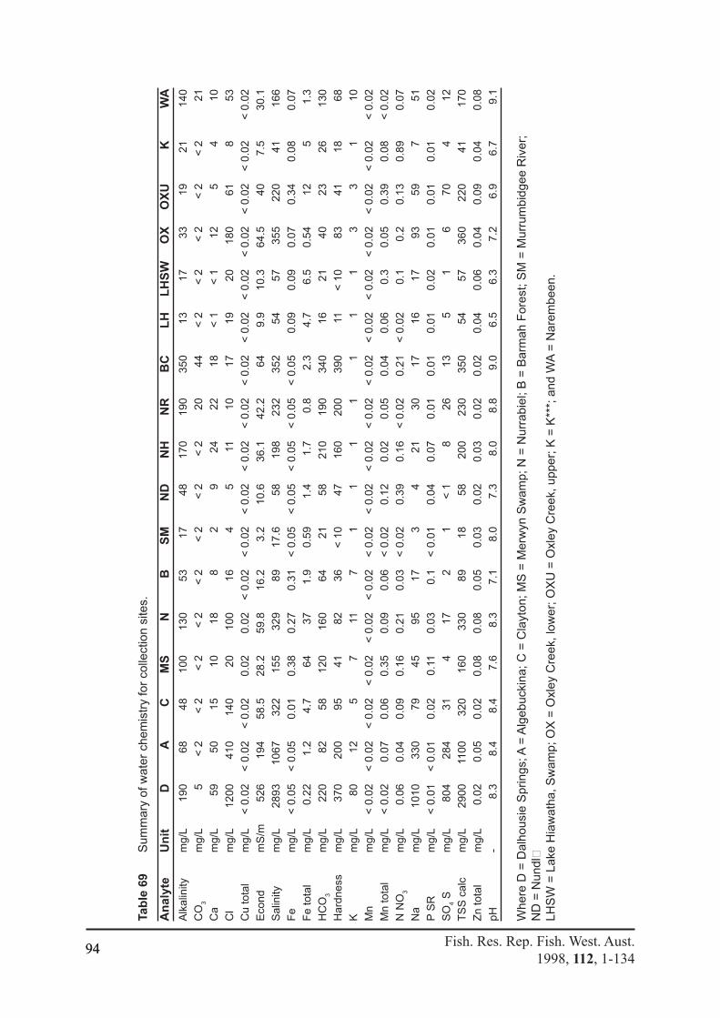
Fish. Res. Rep. Fish. West. Aust.1998, 112, 1-134
94
Tab
le 6
9 S
umm
ary
of w
ater
che
mis
try
for
colle
ctio
n si
tes.
An
alyt
e U
nit
D
A
C
M
S
N
B
SM
N
D
NH
N
R
BC
L
H
LH
SW
O
X
OX
U
K
WA
Alk
alin
ity
mg/
L 19
0 68
48
10
0 13
0 53
17
48
17
0 19
0 35
0 13
17
33
19
21
14
0
CO
3 m
g/L
5 <
2
< 2
<
2
< 2
<
2
< 2
<
2
< 2
20
44
<
2
< 2
<
2
< 2
<
2
21
Ca
mg/
L 59
50
15
10
18
8
2 9
24
22
18
< 1
<
1
12
5 4
10
Cl
mg/
L 12
00
410
140
20
100
16
4 5
11
10
17
19
20
180
61
8 53
Cu
tota
l m
g/L
< 0
.02
< 0
.02
< 0
.02
0.02
0.
02
< 0
.02
< 0
.02
< 0
.02
< 0
.02
< 0
.02
< 0
.02
< 0
.02
< 0
.02
< 0
.02
< 0
.02
< 0
.02
< 0
.02
Eco
nd
mS
/m
526
194
58.5
28
.2
59.8
16
.2
3.2
10.6
36
.1
42.2
64
9.
9 10
.3
64.5
40
7.
5 30
.1
Sal
inity
m
g/L
2893
10
67
322
155
329
89
17.6
58
19
8 23
2 35
2 54
57
35
5 22
0 41
16
6
Fe
mg/
L <
0.0
5 <
0.0
5 0.
01
0.38
0.
27
0.31
<
0.0
5 <
0.0
5 <
0.0
5 <
0.0
5 <
0.0
5 0.
09
0.09
0.
07
0.34
0.
08
0.07
Fe
tota
l m
g/L
0.22
1.
2 4.
7 64
37
1.
9 0.
59
1.4
1.7
0.8
2.3
4.7
6.5
0.54
12
5
1.3
HC
O3
mg/
L 22
0 82
58
12
0 16
0 64
21
58
21
0 19
0 34
0 16
21
40
23
26
13
0
Har
dnes
s m
g/L
370
200
95
41
82
36
< 1
0 47
16
0 20
0 39
0 11
<
10
83
41
18
68
K
mg/
L 80
12
5
7 11
7
1 1
1 1
1 1
1 3
3 1
10
Mn
mg/
L <
0.0
2 <
0.0
2 <
0.0
2 <
0.0
2 <
0.0
2 <
0.0
2 <
0.0
2 <
0.0
2 <
0.0
2 <
0.0
2 <
0.0
2 <
0.0
2 <
0.0
2 <
0.0
2 <
0.0
2 <
0.0
2 <
0.0
2
Mn
tota
l m
g/L
< 0
.02
0.07
0.
06
0.35
0.
09
0.06
<
0.0
2 0.
12
0.02
0.
05
0.04
0.
06
0.3
0.05
0.
39
0.08
<
0.0
2
N N
O3
mg/
L 0.
06
0.04
0.
09
0.16
0.
21
0.03
<
0.0
2 0.
39
0.16
<
0.0
2 0.
21
< 0
.02
0.1
0.2
0.13
0.
89
0.07
Na
mg/
L 10
10
330
79
45
95
17
3 4
21
30
17
16
17
93
59
7 51
P S
R
mg/
L <
0.0
1 <
0.0
1 0.
02
0.11
0.
03
0.1
< 0
.01
0.04
0.
07
0.01
0.
01
0.01
0.
02
0.01
0.
01
0.01
0.
02
SO
4 S
m
g/L
804
284
31
4 17
2
1 <
1
8 26
13
5
1 6
70
4 12
TS
S c
alc
mg/
L 29
00
1100
32
0 16
0 33
0 89
18
58
20
0 23
0 35
0 54
57
36
0 22
0 41
17
0
Zn
tota
l m
g/L
0.02
0.
05
0.02
0.
08
0.08
0.
05
0.03
0.
02
0.03
0.
02
0.02
0.
04
0.06
0.
04
0.09
0.
04
0.08
pH
- 8.
3 8.
4 8.
4 7.
6 8.
3 7.
1 8.
0 7.
3 8.
0 8.
8 9.
0 6.
5 6.
3 7.
2 6.
9 6.
7 9.
1
Whe
re D
= D
alho
usie
Spr
ings
; A =
Alg
ebuc
kina
; C =
Cla
yton
; MS
= M
erw
yn S
wam
p; N
= N
urra
biel
; B =
Bar
mah
For
est;
SM
= M
urru
mbi
dgee
Riv
er;
ND
= N
undl
LH
SW
= L
ake
Hia
wat
ha, S
wam
p; O
X =
Oxl
ey C
reek
, low
er; O
XU
= O
xley
Cre
ek, u
pper
; K =
K**
*; a
nd W
A =
Nar
embe
en.
94
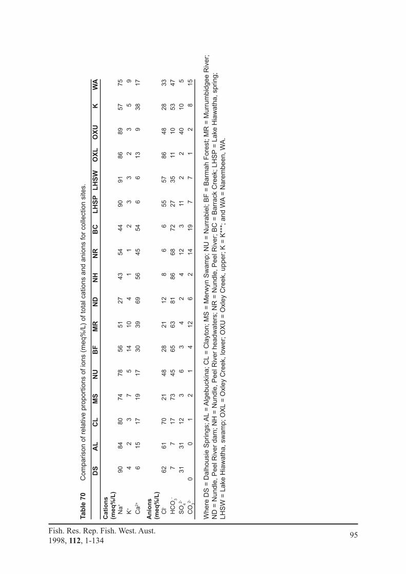
Fish. Res. Rep. Fish. West. Aust.1998, 112, 1-134
95
Tab
le 7
0 C
ompa
rison
of r
elat
ive
prop
ortio
ns o
f ion
s (m
eq%
/L)
of to
tal c
atio
ns a
nd a
nion
s fo
r co
llect
ion
site
s.
D
S
AL
C
L
MS
N
U
BF
M
R
ND
N
H
NR
B
C
LH
SP
L
HS
W
OX
L
OX
U
K
WA
Cat
ion
s (m
eq%
/L)
N
a+
90
84
80
74
78
56
51
27
43
54
44
90
91
86
89
57
75
K
+
4 2
3 7
5 14
10
4
1 1
2 3
3 2
3 5
9
C
a2+
6 15
17
19
17
30
39
69
56
45
54
6
6 13
9
38
17
An
ion
s (m
eq%
/L)
C
l- 62
61
70
21
48
28
21
12
8
6 6
55
57
86
48
28
33
H
CO
3- 7
7 17
73
45
65
63
81
86
68
72
27
35
11
10
53
47
S
O42-
31
31
12
3
6 3
4 2
4 12
3
11
2 2
40
10
5
C
O32-
0
0 1
2 1
4 12
6
2 14
19
7
7 1
2 8
15
Whe
re D
S =
Dal
hous
ie S
prin
gs; A
L =
Alg
ebuc
kina
; CL
= C
layt
on; M
S =
Mer
wyn
Sw
amp;
NU
= N
urra
biel
; BF
= B
arm
ah F
ores
t; M
R =
Mur
rum
bidg
ee R
iver
; N
D =
Nun
dle,
Pee
l Riv
er d
am; N
H =
Nun
dle,
Pee
l Riv
er h
eadw
ater
s; N
R =
Nun
dle,
Pee
l Riv
er; B
C =
Bar
rack
Cre
ek; L
HS
P =
Lak
e H
iaw
atha
, spr
ing;
LH
SW
= L
ake
Hia
wat
ha, s
wam
p; O
XL
= O
xley
Cre
ek, l
ower
; OX
U =
Oxl
ey C
reek
, upp
er; K
= K
***;
and
WA
= N
arem
been
, WA
.

Fish. Res. Rep. Fish. West. Aust. 1998, 112, 1-134
96
Table 71 Summary of combined summer and winter water chemistry (mean, minimum and maximum) recorded from a selection of WA farm dams currently harvested for yabbies (n = 52).
Unit Mean Min Max Alkalinity mg/L 139 16 450 CO3 mg/L 3 < 2 45 Ca mg/L 14 2 44 Cl mg/L 117 15 560 Cu_total mg/L 0.02 < 0.02 0.05 ECond mS/m 68 16 234 Salinity (mg/L) mg/L 375 90 1287 Fe mg/L 0.47 0.05 7.10 Fe_total mg/L 24 0.06 250 HCO3 mg/L 168 19 450 Hardness mg/L 95 16 270 K mg/L 13 5 35 Mn mg/L 0.02 < 0.02 0.05 Mn_total mg/L 0.06 < 0.02 0.46 N_NO3 mg/L 4 0.02 46 Na mg/L 107 20 469 P_SR mg/L 0.30 0.01 5.90 SO4_S mg/L 24 4 81 Zn_total mg/L 0.06 0.02 0.68 pH 7.71 5.00 8.60
Table 72 Comparison of relative proportions of ions (meq%/L) of total cations and anions for a selection of WA farm dams currently harvested for yabbies (n = 52).
meq%/L MEAN MIN MAX Cations Na+ 82 79 87 K+ 6 12 4 Ca2+ 12 9 9 Anions Cl- 50 33 60 HCO3
- 41 35 28 SO4
2- 8 9 6 CO3
2- 1 8 6

Fish. Res. Rep. Fish. West. Aust. 1998, 112, 1-134
97
Dalhousie Springs, SA Dalhousie Springs are Australia’s largest active mound spring complex and are located on the western edge of the Simpson Desert in central Australia. The spring water is of constant temperature and chemistry, and, aside from the ocean, constitutes one of the most stable aquatic environments found on earth (Ponder 1986). The mound springs arise as a result of vertical movement of artesian water, which frequently results in the surface deposition of shale, predominantly calcium carbonate, creating the mound from which they derive their name (Ponder 1986; Armstrong 1990). Although previous publications indicate that there are around 60 springs (Sokol 1987; Horwitz 1990), Dalhousie Springs is actually a collection of 100 springs and mounds of which 80 are active. These springs are spread over an area of 70 km2 (Zeidler and Ponder 1989; A. Ah Chee pers. comm.). While a number of researchers have published papers on yabbies at Dalhousie Springs (Sokol 1987; Horwitz 1990), the last scientific expedition to this region (prior to this one) to collect crayfish was that of Zeidler, who organised a multidisciplinary expedition to this region from 1 to 14 June, 1985. Zeidler’s expedition found crayfish in a total of 24 out of 38 springs (Zeidler 1989). However, in this expedition yabbies were absent from five of six springs which Zeidler had previously found to contain yabbies. In addition, yabbies were absent from nearby Opossum Waterhole and Dalhousie Homestead springs.
The yabbies collected by our expedition to Dalhousie Springs came from a remote spring, surrounded by desert and inaccessible by 4WD vehicle, so the likelihood of translocation is extremely remote. The yabbies were collected by hand scoop net from the dense algal mat on the bottom of this shallow spring (Table 68). There was no evidence of burrows in this location. Yabbies from Dalhousie Springs were considered by Sokol (1987), to be an intermediate form between C. destructor and C. albidus, based upon the areolar width, and, although inhabiting what is now an essentially arid region, may be relics from a wetter climate in the tertiary period (Boyd 1990; Ponder 1986). Sokol (1987) further proposed that these animals may represent an undescribed species of yabby.
The yabbies at Dalhousie Springs have received considerable attention due to their reputed ability to withstand high temperatures up to 44°C (Sokol 1987; Horwitz 1990; Horwitz and Knott 1995). The optimum temperature reported for growth of yabbies (C. destructor) is 28°C and growth ceases over 34°C (Merrick and Lambert 1991; Mills 1983; Morrissy et al. 1990). At their vents, the mound springs at Dalhousie range in temperature from 30° to 46°C and in contrast to the reports of Sokol (1987) and Horwitz (1990), our expedition found yabbies only in the cooler out-flow channels with temperatures of 17.6°C (Table 68). This agrees with the findings of the previous expedition by Zeidler which only found yabbies in the cool drain channels (Zeidler 1989; W. Zeidler pers. comm.).
Ground water reaching the surface at Dalhousie is generally low in dissolved oxygen (DO), but rapidly becomes saturated, as demonstrated by the high DO level (9.55 mg/L) recorded (Table 68). In common with farm dams in Western Australia, Dalhousie Springs, being in the western group of the Lake Eyre supergroup, are sodium chloride dominated with a low bicarbonate component and relatively high levels of sulphate (Tables 69, 70, 71 and 72).
The Dalhousie strain of yabbies therefore represents an ecotype which has evolved in permanent waters of high NaCl dominated salinity, similar to the south-west of WA. The

Fish. Res. Rep. Fish. West. Aust. 1998, 112, 1-134
98
upper level of salinity tolerance at which yabbies maintain normal behaviour, is reported to be 12,000 mg/L (Mills and Geddes 1980). The salinity recorded at this location (2,893 mg/L), is considerably higher than the maximum salinity recorded for yabby dams in production in WA (1,287 mg/L) (Tables 69 and 71), but well below the upper limit of salinity tolerance reported for yabbies.
The water in this habitat is very clear, shelter from predators is provided by a dense algal mat formed by what appeared to be the stonewort Chara sp. into which these yabbies burrow.
This variety of yabby may have relevance to aquaculture as a result of evolving in a habitat which requires a high salinity tolerance, while not requiring burrowing or high levels of seasonal reproduction to ensure that populations survive drought. Although the largest mound spring group, Dalhousie is only one of many groups of permanent springs in central Australia and a more comprehensive expedition is likely to discover additional strains of yabbies which may have evolved physical adaptations relevant to inland aquaculture, particularly in saline or arid regions. Algebuckina, SA The Algebuckina waterhole is a large permanent water body on the Neales River, north of Oodnadatta. The waterhole has steep banks leading into a relatively exposed, turbid, stretch of water. Yabbies were collected by baited traps. As opposed to the purely artesian water source in Dalhousie Springs, the Algebuckina waterhole is also filled by the Neales River, which arises in central Australia and discharges into Lake Eyre (Armstrong 1990). The high salinity of the water (1,067 mg/L) (Table 69) comes from nearby artesian springs, which flow into the Algebuckina waterhole. In common with Dalhousie Springs, this water is sodium chloride dominated with a low bicarbonate component and relatively high sulphate levels which are similar to saline dams in Western Australia (Tables 69, 70, 71 and 72).
The yabby population in the Algebuckina waterhole therefore survives in a permanent but chemically variable habitat which, like WA farm dams, ranges from fresh after recent rains through to saline during periods of drought. However, yabbies have not been reported in Lake Eyre, when the vast salt pan fills (Williams 1990), therefore this yabby variety is restricted, most likely due to salinity, to the upper reaches of the Neales River.
Clayton, SA Clayton is located on the western edge of Lake Alexandrina, at the mouth of the Murray River. The sampling locality is a permanent, broad expanse of water with little shelter which is exposed to prevailing coastal winds and has a mild climate.
Yabbies are fished commercially from Lake Alexandrina between October and April each year. Yabbies suffered a major population crash in the early 1970s with the dispersal of the introduced carp to this locality. The yabbies collected from Clayton represent C. destructor from Lake Alexandrina at the mouth of the Murray River. This corresponds with Sokol’s (1987) collection locality in Lake Alexandrina (locality DE21), which he described as C. destructor and later confirmed by Campbell et al. (1994) at locality LA in the same area. This water, like that of farm dams in Western Australia, is NaCl dominated but in comparison with the above more inland habitats in SA, it is relatively low in sulphate (Tables 68 and 69).

Fish. Res. Rep. Fish. West. Aust. 1998, 112, 1-134
99
Merwyn Swamp, Vic Although yabbies had previously been thought to have been translocated to Western Australia from a “Miram Swamp”, it became clear that the correct source location is Merwyn Swamp, located south of the town of Miram. In February 1927, Ivan Smith (1897-1973) moved from his family’s property, which bordered Merwyn Swamp, to Bruce Rock then later to Narembeen, Western Australia. He returned briefly to Miram to attend a wedding in August 1932. When Ivan Smith returned to Narembeen, Western Australia, he brought with him 10 yabbies from Merwyn Swamp in a wet hessian bag placed in a kerosene tin (M. Bristow pers. comm.). This was confirmed by the records from the Wheaton family store, which go back over 100 years (H. Wheaton pers. comm.; L. Wheaton pers. comm.; Merret 1979). These yabbies were placed into a small dam near Ivan Smith’s house. In early January 1935, Ivan Smith’s house dam went dry. Frank Bristow and Ivan Smith collected eight yabbies from the mud, these were stocked into a dam on Frank Bristow’s property and, as the population grew, they were distributed to farmers throughout the Narembeen, Bruce Rock, Bonnie Rock and also Bencubbin district (M. Bristow pers. comm.; Morrissy and Cassells 1992). Merwyn Swamp is a shallow turbid, heavily wooded swamp, south of the small town of Miram in the Wimmera region of Victoria. Merwyn Swamp is bordered to the north by the Big Desert and to the south by the Little Desert.
Merwyn Swamp is an ephemeral swamp where the yabbies must burrow during summer to avoid desiccation when the water evaporates. This environment is one which would favour an “r” selected species capable of producing large numbers of juveniles within a short period of time when water returns.
The general topography, latitude and land use in the Merwyn Swamp district is similar to that of the Wheatbelt in Western Australia (Table 73).
Table 73 Environmental parameters for Narrambeen, WA and Merwyn Swamp, Vic.
Characteristic Merwyn Swamp (Vic.) Narrambeen (WA) Latitude 36° 21′ south 32° 4′ south Altitude (m) 101 276 Temperature range Max (mean) 21.6 24.8 Min (mean) 8.0 10.5 Rainfall mean (mm) 421 332 Topography Flat Flat Land use Crops Wheat and sheep Soil type Clay Clay
However, unlike most Wheatbelt farm dams, the water in Merwyn Swamp is dominated by sodium and hydrogen bicarbonate, not sodium chloride (Table 70 and 72). Of particular interest is the calcium level recorded for Merwyn Swamp, which is similar to the average of harvested farm dams in WA; as are most environmental and important chemical parameters (i.e. electrical conductivity, salinity, hydrogen carbonates, sodium and total zinc) we recorded at this locality (Tables 69 and 71). Variability in chemistry between these sites was displayed by parameters that typically vary widely through the day (i.e. alkalinity, carbonates, hardness and pH). However, as both Merwyn Swamp and Narembeen were sampled in the morning, the large differences in pH and carbonate may have significance to yabby production in

Fish. Res. Rep. Fish. West. Aust. 1998, 112, 1-134
100
Wheatbelt farm dams (Table 69). Similarly there were large differences in iron, manganese and phosphorus between Merwyn Swamp and Narembeen, although these parameters were still within the range recorded from WA farm dams (Tables 69 and 71). Nurrabiel, Vic The Nurrabiel water body is very similar to Merwyn Swamp, i.e. a shallow, turbid lake fringed by partially submerged trees. Nurrabiel, Victoria is the type locality designated by Clark (1936) for C. albidus. The yabbies from this site were also included on Sokol’s (1988) study (locality Al11), in which he described them as C. albidus. Samples collected from this locality by Sokol were also used in Austin’s study (locality NUR) who designated them as C. destructor-albidus (Austin 1987). In this region local residents refer to C. albidus as the “White Yabby”, so as to distinguish them from the common yabby, C. destructor. Barmah Forest, Vic The Barmah Forest is located in northern Victoria on the edge of the Murray River. This is a series of inter-connecting swamps, subject to annual flooding through predominantly redgum forest. These swamps drain into the Barmah Lakes and the Murray River. The Barmah Lakes are also connected to the Moira Irrigation Scheme. Two types of yabby were collected from this region, one was the typical C. destructor and the other an undescribed species easily distinguished from C. destructor by its broad chelae and dense setae on the ventral surface of these claws. The first of these undescribed yabbies were caught by locals in 1991 as the floods of that year receded (F. Piper pers. comm.). However, they may also have been collected previously in 1963 and 1983, as they closely fit the description provided by Sokol (1988). Austin (1996) proposes that these two samples included in Sokol’s (1988) analyses of C. rotundus, represent an undescribed species of Cherax from central Victoria and can be distinguished by electrophoresis (Austin 1996) (section 5.1). Local collectors report that the “normal” C. destructor is usually found in the lakes, creeks and irrigation canals; while the undescribed Cherax sp. is more common in the ephemeral swamps. The “new” species of Cherax is thought to burrow in the swamp, but it is “washed” into creeks and lakes as a result of annual flooding. These yabbies are only present in traps when, or soon after, the forest has been flooded (F. Piper pers. comm.). Large numbers of C. destructor could be obtained by placing traps where water was flowing. i.e. under a waterfall or weir. A large number of burrows were observed in the irrigation canal banks. Upon excavation many of these burrows were occupied at water level. However, all burrows excavated were a u-shape, with openings above and below the water level. The maximum depth of these burrows was 50 cm. In comparison to other C. destructor destructor habitats, the water in the Barmah Forest is acidic and is relatively high in iron (Table 69).

Fish. Res. Rep. Fish. West. Aust. 1998, 112, 1-134
101
Murrumbidgee River, NSW The head waters of the Murrumbidgee River location represent an alpine ecotype in the Great Dividing Range. This area is subject to regular snow falls with relatively low summer temperatures. The headwaters of the Murrumbidgee River support one of the highest and most easterly populations of C. destructor (Figure 31, Table 68).
As expected for an alpine stream, this locality is characterised by clear rapid flowing water (Tables 68 and 69). The water chemistry demonstrates that this area has low calcium and very low salinity. The water is sodium and hydrogen carbonate dominated and has low hardness.
Nundle, NSW The Peel River in Nundle is the type locality for C. esculus, which has only been reported from this locality (Reik 1956, 1969). Sokol (1988) analysed the putative C. esculus type-specimens that Reik had placed in the Australian Museum and synonymised C. esculus with C. destructor. Austin (1996) did not examine this species in his study due to the remoteness of its recorded distribution. Consequently, no other researchers have sampled the C. esculus type locality since Reik (1956). The Peel River runs west from the Great Dividing Range. Yabbies were collected from three areas on the Peel River: Sheba dam, the river headwaters, and the low lying river after it exits the town of Nundle.
Yabbies were trapped and collected by hand from the headwaters. In the lower reaches of the river, no yabbies were found, however, tortoises were trapped and there were signs of platypus. In comparison to the other collecting localities, the Peel River has a high alkalinity (Table 69), however, this is well within the range recorded in Western Australian farm dams (Table 71). This river is calcium dominated in its upper reaches and sodium dominated in the lower reaches. Barrack Creek, NSW Barrack Creek is located in the Upper Bingarra goldfields, NSW. This is a rapid flowing shallow spring-fed creek. The spring arises in a limestone cave and has eroded a course through the limestone. This is reflected in the water chemistry, particularly high levels of alkalinity, hardness and pH (Table 69).
Due to the solid rock creek bed, the yabbies are unable to burrow and instead were found under ledges or hidden under weed. The depth of this creek ranged from 1 to 60 cm in the area sampled. The size of yabbies from this shallow spring (like those of Dalhousie Springs) were small (section 5.3). Lake Hiawatha, NSW Lake Hiawatha is 315 ha in area and is a unique coastal water body. It is a large permanent body of freshwater located in northern NSW. The lake is not filled by surface run-off, but rather via a deep aquifer in the bottom of the lake’s western area. Although the type locality for C. cuspidatus is Heron Creek, 20 miles south of Port Macquarie (Reik 1969), the first specimens of C. cuspidatus were actually obtained from the outlet of Lake Hiawatha in 1954 by Dr A.A. Racek, who sent them to Edgar Reik for identification (Dr A.A. Racek pers. comm.). Some confusion has arisen as to the exact location of Lake Hiawatha due to the original description for C. cuspidatus stating that it is west of Grafton,

Fish. Res. Rep. Fish. West. Aust. 1998, 112, 1-134
102
when it is actually east of Grafton (Reik 1969). Austin (1987) sampled C. cuspidatus from 2 km west of Lake Hiawatha, this coincides with Bookram Creek, just prior to entering the tidal Wooli Wooli River estuary. The sampling site of C. cuspidatus by Austin (locality LAH) is therefore different from that of the original collection locality reported by Reik, using the specimens provided by Dr A.A. Racek.
No yabbies were collected from Austin’s (1987) locality LAH, this is most likely due to the high tidal salinity of over 15 parts per thousand (ppt) recorded from this location.
Yabbies were collected from a spring on the high western edge of the lake and a neighbouring swamp created by the out-flow from the spring which then drains into Lake Hiawatha. No yabbies were caught in the main lake, the out-flows from the lake (which had recently been the site of a bushfire) or the neighbouring Minnie Waters. Many tortoises were found in the main lake and pygmy perch and rainbow fish in Minnie Waters. Lake Hiawatha is a permanent water body which, in comparison to farm dams, has very low calcium levels, alkalinity, hydrogen carbonate, hardness and pH. The water in Lake Hiawatha is sodium chloride dominated.
Oxley Creek, Qld Sandy Creek, Marooka, Brisbane is the type locality for C. dispar (Reik 1951); however, Sandy Creek now has a waste water treatment plant which releases into the creek and this has resulted in dark anaerobic sediments down stream from the plant. While no water was present up stream (i.e. entire flow was due to treated waste water), no yabbies were found in this locality.
Although no Cherax were found in Sandy Creek, the type locality for this species, they were obtained from Oxley Creek, less than 7 km from Sandy Creek, which had previously been sampled by Austin (1996) (locality OXL). Oxley Creek is a slow flowing warm-water river. At the time of sampling, however, Oxley Creek was being mined for sand by Readymix. Water chemistry presented in Table 62 indicates that parameters vary between sample sites upstream (locality OXU) and downstream (locality OXL) from the sand mining. Although C. dispar from this location was only found in small numbers, they did occur both above and below the sand mining operation. K***, NSW This spring near K*** is a small permanent water body surrounded by dense vegetation. Yabbies were collected from both the spring and resulting over-flow, by using traps and hand scoop nets. The water from the spring was turbid and had a very low salinity (41 mg/L) (Table 69).
Narembeen, WA Narembeen is the locality in WA to which yabbies were reported to have been translocated by Ivan Smith in 1932. Unlike Merwyn Swamp this is a man-made farm dam. In this region, farmers report a high production problem, with females producing large numbers of juveniles which stunt (M. Bristow pers. comm.).

Fish. Res. Rep. Fish. West. Aust. 1998, 112, 1-134
103
Discussion
In this study, yabbies have been sampled from a wide variety of ecotypes including desert mound springs, inland billabongs, alpine streams, river mouths, swamps, lakes, headwater springs, subtropical springs and creeks. It is clear that some regions have varieties of yabbies which are more suited environmentally to the arid regions of Western Australia. It is fortuitous that the animals introduced from Merwyn Swamp originated in a region that is very similar, in terms of the important chemical and environmental aspects, to the Western Australian Wheatbelt situation. This, in part, must be considered to be a major contributing factor to the rapid multiplication of the original the yabbies, the offspring of which are now farmed over an area greater than 750,000 km2 in WA.
Tables 68-72, indicate that water quality is within the ranges well tolerated by freshwater species (Langdon 1988) and, in addition, there does not appear to be a fundamental chemical difference between the original locality and WA waterbodies which would limit the growth of yabbies in WA farm dams. Therefore, while four possible reasons for the stunting of yabby stocks in farm dams in WA have been proposed (namely: over-population due to an “r” selected species being stocked into a permanent waterbody; inbreeding resulting in a genetic bottleneck; limiting environmental factors; and differences in water chemistry between type localities and WA), the water chemistry variation between WA and Merwyn Swamp does not appear to be a major factor. The most consistent factor which resulted in the absence of yabbies, was when eels and tortoises were present in the eastern native localities. Where rivers contained eels and tortoises, yabbies were confined to the headwater springs and the individuals were of small size, unlike inland stocks, the exception being the microhabitat of Dalhousie Springs. A large number of habitats of the putative species and strains of the “yabby complex” are currently under pressure due to the impact of man. The mechanisms by which man has an impact upon yabby ecosystems may be either direct, such as sand mining, urban sprawl or sewerage outfalls, or indirect, such as the introduction of carp, increasing salinization due to land clearing or the grazing of cattle on mound springs. In particular, a number of the type localities, recorded for putative species of the “yabby complex”, and some of the collection localities, of previous researchers, no longer exist or have been severely degraded. Most of the locations sampled represent “varieties” of yabbies which have previously been the subject of taxonomic investigations (Austin 1987, 1988; Reik 1951, 1956, 1969; Sokol 1987, 1988). However, a future taxonomic study to confirm the identity of the species actually collected during this expedition would add considerably to our current knowledge of the habitats and selection of suitable yabby species for aquaculture. Until the animals collected for this study have been classified by a taxonomist, the yabby “varieties” collected will be referred to according to their collection locality rather than a putative species name, both in the following chapters and in future publications.
Fish. Res. Rep. Fish. West. Aust. 1998, 112, 1-134
104
References
Armstrong, D. 1990. Hydrology. In Tyler, M.J., Twidale, C.R., Davies, M. and Wells, C.B. (eds.) Natural history of the north east deserts, Royal Society of SA, pp. 75-80.
Austin, C.M. 1987. Electrophoretic and morphological systematic studies of the genus Cherax (Decapoda: Parastacidae) in Australia. PhD thesis, University of Western Australia.
Austin, C.M. 1996. Systematics of the freshwater crayfish genus Cherax Erichson (Decapoda: Parastacidae) in northern and eastern Australia: electrophoretic and morphological variation. Aust. J. Zool., 44: 259-296.
Bayley, I.A.E. and Williams, W.D. 1973. Inland waters and their ecology. Longman Cheshire, Melbourne, 314p.
Campbell, N.J.H., Geddes, M.C. and Adams, M. 1994. Genetic variation in yabbies Cherax destructor and C. albidus (Crustacea: Decapoda: Parastacidae), indicates the presence of a single highly sub-structured species. Aust. J. Zool. 42: 745-760.
Clark, E. 1936. The freshwater and land crayfishes of Australia. Mem. Nat. Mus. Vict., 10: 5-58.
Clark, E. 1941. New species of Australian freshwater and land crayfishes (Family Parastacidae) Mem. Nat. Mus. Vict., 12: 31-41.
Francesconi, K.A., Morrissy, N.M., Fellows, C.J. and Bird, C. 1995. Survey of marron farms and the marron recreational fishery in Western Australia for pesticides and water chemistry, with related laboratory experimentation. Fisheries Research Bulletin No. 30. Fisheries Department of WA, 14p.
Horwitz, P. 1990. The conservation status of Australian freshwater crustacea. 121p. Horwitz, P. and Knott, B. 1995. The distribution and spread of the yabby Cherax destructor
complex in Australia: speculations, hypotheses and the need for research. In Geddes, M., Fielder, D. and Richardson, A. (eds.) Freshwater Crayfish, 10: 81-91.
Langdon, J.S. 1989. Environment and management factors in diseases of fish In Bryden, D.I. (ed.) Fish Disease: Refresher Course for Veterinarians. Postgraduate committee in Veterinary Science, University of Sydney, pp. 329-353.
Merrick, J.R. and Lambert, C.N. 1991. The Yabby, Marron and Red Claw Production and Marketing, JR Merrick Productions, Artarmon, NSW, 80p.
Mills, B.J. 1983. Aquaculture of yabbies. Proceedings of the first Freshwater Aquaculture Workshop. Dept. of Agriculture, NSW, pp. 89-98.
Mills, B.J. and Geddes, M.C. 1980. Salinity tolerance and osmoregulation of the Australian freshwater crayfish Cherax destructor Clark (Decapoda: Parastacidae). Aust. J. Mar. Freshwater Res., 31: 667-676.
Merret, L. 1979. Family history of James Smith 1829-1910 and his wife Alice Twining 1841-1926. Lutheran Publishing House, 306p.
Morrissy, N.M., Evans, L. and Huner, J.V. 1990. Australian freshwater crayfish: Aquaculture species. World Aquaculture 21(2): 113-122.

Fish. Res. Rep. Fish. West. Aust. 1998, 112, 1-134
105
Morrissy, N.M and Cassells, G. 1992. Spread of the introduced yabby Cherax albidus Clark 1936 in Western Australia. Fisheries Research Report No. 92, Fisheries Department of WA, 27p.
Ponder, W.F. 1986. Mound springs of the Great Artesian Basin. In De Deckker, P. (ed.) Limnology in Australia, pp. 403-420.
Reik, E.F. 1951. The freshwater crayfish (Family Parastacidae) of Queensland, Rec. Aus. Mus. 22: 368-388.
Reik, E.F. 1956. Additions to the Australian freshwater crayfish. Rec. Aus. Mus., 24: 1-7.
Reik, E.F. 1969. The Australian freshwater crayfish (Crustacea: Decapoda: Parastacidae), with definitions of new species. Aust. J. Zool., 17: 855-918.
Sokol, A. 1987. Yabbies at Dalhousie Springs, northern South Australia: morphological evidence for long term isolation. Transcripts of the Royal Society of South Australia. 3: 207-209.
Sokol, A. 1988. Morphological variation in relation to the taxonomy of the destructor group of the genus Cherax. Invertebr. Taxon., 2: 55-79.
Williams, W.D. 1990. Salt lakes: The limnology of Lake Eyre. In Tyler, M.J., Twidale, C.R., Davies, M. and Wells, C.B. (eds.) Natural history of the north east deserts. Royal Society of SA. pp. 85-99.
Zielder, W. 1982. South Australian freshwater crayfish. South Australian Naturalist. 56(3): 36-43.
Zeidler, W. 1989. Crustacea. In Zeidler, W. and Ponder, W.F. (eds.) Natural History of Dalhousie Springs. South Australian Museum Adelaide, pp. 79-88.
Zeidler, W. and Ponder, W.F. 1989. Natural History of Dalhousie Springs. South Australian Museum Adelaide, 138p.
5.3 The size of yabbies from different localities throughout Australia Introduction
Most previous studies on the morphology of different “varieties” of yabbies have concentrated upon the taxonomy of the genus Cherax (see section 5.1), using either morphological or biochemical variation to discriminate between species (Clark 1936, 1941; Reik 1951, 1969; Sokol 1988; Campbell et al. 1994; Austin 1996).
Species are often subdivided into local populations or demes and substantial genetic differences may evolve among demes which have limited gene exchange (Hedgecock et al. 1979). Previous studies have shown that isolated populations of freshwater crayfish of the same species (Astacus astacus) and from the same ancestral population, can show changes in morphology after being separated for less than a century (Fevolden and Hessen 1989).
Genotypic variation is the genetic makeup of the individual, while phenotypic variance refers to the observed variation and is composed of both genetic and environmental sources of variation. Therefore, while allopatric populations of yabbies may have genetic variation, they may also show phenotypic variation as a result of their surrounding environment. Aim

Fish. Res. Rep. Fish. West. Aust. 1998, 112, 1-134
106
From the yabby aquaculture industry’s point of view, the major factor overlooked by previous taxonomic studies is whether the average size of yabbies varies according to different species or geographical varieties. Body weight is the main factor of importance to the aquaculture industry as yabbies are graded according to weight and condition. Although weight grades and prices vary around Australia, yabbies below 30 g are considered by industry to be of no commercial value. Most processors pay higher prices for larger yabbies, which reflects the demand for larger crayfish and the greater difficulty in producing large yabbies. Materials and methods
Yabbies were collected from sites according to the methods presented previously in sections 2.3 and 5.2.
Immediately after capture, yabbies from each collection locality were weighed using a Sartorius balance and the weights were recorded to two significant figures. To account for possible skewed size distributions due to different collecting techniques (i.e. trapping, hand net, seine net, hand collection) and the effect of environmental conditions which may have limited the maximum size of animals from each locality (i.e. water depth, feed, density), yabbies were held in aquaria for two years under homogeneous conditions. The animals were weighed at the conclusion of the study to record the maximum size of yabbies from each population. Results
The mean weight of yabbies from most collection sites was below 30 g, which is the minimum weight grade considered to be of commercial value (Tables 73 and 74). Consequently, commercial harvesting of yabbies from most of the localities sampled in this study is unlikely to be economically viable. Table 74 Size grade and average farm-gate price for yabbies from collection localities.
Locality Size grade Farm-gate price (mean) ($/kg) Dalhousie Springs below 30 g No commercial value Algebuckina “ “ Nurrabiel “ “ Murrumbidgee River “ “ Nundle “ “ Barrack Creek “ “ Lake Hiawatha “ “ Oxley Creek “ “ K*** “ “ Clayton 30-40 g 5.00 Narembeen 40-50 g 7.00 Barmah Forest 50-60 g 8.00 - 60-70 g 9.00 Merwyn Swamp 70-80 g 10.00

Fish. Res. Rep. Fish. West. Aust. 1998, 112, 1-134
107
Although yabbies from Narembeen, WA are reported to have come from Merwyn Swamp, Vic, they appear, on average to be smaller than animals from the ancestral population (Tables 74 and 75). In the Narembeen region, farmers report a high production problem, with females producing large numbers of juveniles which stunt (M.. Bristow pers. comm.). This may be the result of a high level of inbreeding (due to the low number of original broodstock-eight animals), selection pressure due to trapping (section 3.7) and/or environmental conditions which may have contributed to stunting in the population from the Narembeen collection site. These results should, however, be confirmed on a larger scale to determine if the lower sizes are specific to the dam sampled and, if this is the case, if populations from other regions within WA are larger in size than those in the Narembeen locality. Table 75 Localities, mean, minimum and maximum body weights, and collection methods for yabbies.
Location Mean (g) Min (g) Max (g) Collection Method n Dalhousie Springs 6 1 24 hand and scoop net 23 Algebuckina 29 8 71 traps 26 Clayton 34 5 130 traps 23 Merwyn Swamp 74 41 74 traps 41 Nurrabiel 15 5 89 traps 141 Barmah Forest 55 5 146 traps 118 Murrumbidgee River 27 14 51 traps 4 Nundle 19 2. 72 traps and hand 31 Barrack Creek 5 1 16 hand and scoop net 42 Lake Hiawatha 6 1 14 traps and scoop net 129 Oxley Creek 10 10 11 traps 6 K*** 8 2 23 traps, scoop net and seine 91 Narembeen 48 33 63 traps 86
Trapping proved an effective method for collecting a large size range of animals (1-146 g) (Table 75). However, the size selectivity of trapping for each of the populations sampled is not known. In general, smaller yabbies were collected by hand or with scoop nets while larger animals were caught in traps. Alternatively, the collection of larger animals by trapping may be due to environmental limitations, such as predation and water depth, as the selection of sampling technique was dictated by the water depth. In shallow waters (below 30 cm) traps could not be submerged so animals were collected by hand; while in deeper waters hand collection was often not practical, so trapping was the most successful technique. Furthermore, in waters with a gradual slope or with a maximum depth between 30-100 cm, trapping, scoop net and seine net could be used. Even after two years in aquaria, yabbies from Lake Hiawatha and Oxley Creek failed to reach a minimum market size of 30 g (Table 76). Although the weight of yabbies grown in aquarium trials gives some indication of relative sizes of varieties of crayfish, these values must be interpreted with caution as growth and size is affected by density, and reduced growth in aquaria has been recorded in comparison to pond systems.
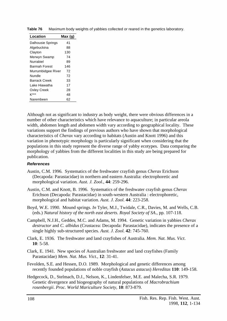
Fish. Res. Rep. Fish. West. Aust. 1998, 112, 1-134
108
Table 76 Maximum body weights of yabbies collected or reared in the genetics laboratory.
Location Max (g) Dalhousie Springs 41 Algebuckina 88 Clayton 130 Merwyn Swamp 74 Nurrabiel 89 Barmah Forest 146 Murrumbidgee River 72 Nundle 72 Barrack Creek 33 Lake Hiawatha 17 Oxley Creek 28 K*** 48 Narembeen 62
Although not as significant to industry as body weight, there were obvious differences in a number of other characteristics which have relevance to aquaculture; in particular areola width, abdomen length and abdomen width vary according to geographical locality. These variations support the findings of previous authors who have shown that morphological characteristics of Cherax vary according to habitats (Austin and Knott 1996) and this variation in phenotypic morphology is particularly significant when considering that the populations in this study represent the diverse range of yabby ecotypes. Data comparing the morphology of yabbies from the different localities in this study are being prepared for publication. References
Austin, C.M. 1996. Systematics of the freshwater crayfish genus Cherax Erichson (Decapoda: Parastacidae) in northern and eastern Australia: electrophoretic and morphological variation. Aust. J. Zool., 44: 259-296.
Austin, C.M. and Knott, B. 1996. Systematics of the freshwater crayfish genus Cherax Erichson (Decapoda: Parastacidae) in south-western Australia : electrophoretic, morphological and habitat variation. Aust. J. Zool. 44: 223-258.
Boyd, W.E. 1990. Mound springs. In Tyler, M.J., Twidale, C.R., Davies, M. and Wells, C.B. (eds.) Natural history of the north east deserts. Royal Society of SA., pp. 107-118.
Campbell, N.J.H., Geddes, M.C. and Adams, M. 1994. Genetic variation in yabbies Cherax destructor and C. albidus (Crustacea: Decapoda: Parastacidae), indicates the presence of a single highly sub-structured species. Aust. J. Zool. 42: 745-760.
Clark, E. 1936. The freshwater and land crayfishes of Australia. Mem. Nat. Mus. Vict. 10: 5-58.
Clark, E. 1941. New species of Australian freshwater and land crayfishes (Family Parastacidae) Mem. Nat. Mus. Vict., 12: 31-41.
Fevolden, S.E. and Hessen, D.O. 1989. Morphological and genetic differences among recently founded populations of noble crayfish (Astacus astacus) Hereditas 110: 149-158.
Hedgecock, D., Stelmach, D.J., Nelson, K., Lindenfelser, M.E. and Malecha, S.R. 1979. Genetic divergence and biogeography of natural populations of Macrobrachium rosenbergii. Proc. World Mariculture Society, 10: 873-879.

Fish. Res. Rep. Fish. West. Aust. 1998, 112, 1-134
109
Ponder, W.F. 1986. Mound springs of the Great Artesian Basin. In De Deckker, P. (ed.) Limnology in Australia. pp. 403-420.
Reik, E.F. 1951. The freshwater crayfish (Family Parastacidae) of Queensland. Rec. Aus. Mus. 22: 368-388.
Reik, E.F. 1969. The Australian freshwater crayfish (Crustacea: Decapoda: Parastacidae), with definitions of new species. Aust. J. Zool., 17: 855-918.
Sokol, A. 1987. Yabbies at Dalhousie Springs, northern South Australia: morphological evidence for long term isolation. Transcripts of the Royal Society of South Australia. 3: 207-209.
Sokol, A. 1988. Morphological variation in relation to the taxonomy of the destructor group of the genus Cherax. Invertebr. Taxon., 2: 55-79.
B) The size at sexual maturity and sex ratio of selected yabby strains 5.4 Size at sexual maturity Introduction
In contrast to permanent waterbodies with a constant environment, fluctuating environments such as farm dams, favour r-strategist species or strains, in which age and size at first reproduction are respectively lower and smaller (Stearns 1976). In farm dams, this uncontrolled reproduction of yabbies results in increased densities and consequently stunted populations.
One approach to controlling reproduction is to harvest animals prior to sexual maturity. This requires the selection of a strain or species which reaches sexual maturity at a larger size, preferably above 30 g, the minimum market size for yabbies. Size at sexual maturity has been reported to vary between populations of freshwater crayfish species including P. Clarkii (Huner and Romaire 1978) and Euastacus bispinosus (Honan and Mitchell 1995). Evidence exists which supports the hypothesis that the size of sexual maturity, as determined by the smallest berried females recorded in a population, varies between localities (Faragher 1983; Johnson 1979; Lewis 1976; Mills and McCloud 1983; Reynolds 1980; Sokol 1987; Woodland 1967). The smallest recorded size at sexual maturity for a yabby is for the strain from Dalhousie Springs, with an orbit carapace length (OCL) of 19.8 mm (Sokol 1987). While the smallest minimum size of berried females in a population of C. destructor from western NSW was an OCL of 38.8 mm (Reynolds 1980).
A study of farm dams in the Pingelly region of the WA Wheatbelt showed that on average, female yabbies mature at approximately 20 g (5 s.e.) (Morrissy pers. comm.). According to a weight-length relationship based upon measurements of over 5,000 yabbies from WA, this equates to an OCL of around 32 mm (Figure 32).

Fish. Res. Rep. Fish. West. Aust. 1998, 112, 1-134
110
y = 0.0006x3.0107
R2 = 0.9061
0
10
20
30
40
50
60
70
80
0 10 20 30 40 50
O CL (mm)
WEI
GHT
(g)
Figure 32 Weight (g)-length (OCL mm) relationship for WA yabbies.
As size at sexual maturity in decapods may be due to genetic and/or environmental factors, the age and size at sexual maturity of the yabby strains were compared in a controlled environment within the Reproduction and Genetics Laboratory.
Aim
To record the minimum size at sexual maturity of yabbies from different localities under homogeneous conditions. Materials and methods
Yabbies were collected and maintained according to the methods described previously in section 2.
As it has been shown that morphological changes for other species of decapods do not always correlate with functional sexual maturity (Aiken and Waddy 1980; Wenner et al. 1985) and to permit comparison with the results of previous researchers, the minimum age/size at sexual maturity was recorded as the age/size at which females in mixed-sex population tanks first became berried. Size and age at sexual maturity was recorded by measuring weight and OCL of F1 generation berried females from breeding populations of each strain over a period of three years. Results
The minimum age and size of berried females varied between populations under controlled homogeneous conditions. Yabbies from Oxley Creek had the smallest size at sexual maturity, while animals from Nurrabiel had the largest minimum size at first berry (Figure 33).

Fish. Res. Rep. Fish. West. Aust. 1998, 112, 1-134
111
0
5
10
15
20
25
30
35
OXLE
YCR
EEK
DALH
OUSIE
LAKE
HIAWA
THA WA
MERW
YNSW
AMP
BARM
AH K***
BARR
ACK
CREE
K
NURR
ABRIE
L
STRAIN
OCL A
T SEX
UAL M
ATUR
ITY (m
m)
Figure 33 Minimum size (OCL) of berried females from nine localities.
The smallest size previously recorded for a berried female yabby is an OCL of 19.8 mm (Sokol 1987). In this study the smallest size for a berried female was 15.53 mm OCL, from Oxley Creek, which is from the dispar group. The minimum size recorded for a berried female from the destructor group was 17.17 mm OCL, from Dalhousie Springs, which is over 2.5 mm less than the previously reported minimum size for a berried female “destructor” yabby (Sokol 1987) (Table 77). No strains reached first berry at above the current minimum market size of 30 g (Table 77).
Table 77 Minimum size and age of berried females from nine localities.
Strain OCL (mm) Weight (g) Age (months) Oxley Creek 15.53 3 10 Dalhousie 17.17 3 9 Lake Hiawatha 17.87 3 6 WA 24.36 10 5 Merwyn Swamp 25.33 12 9 Barmah 27.93 9 4 K*** 29.36 12 7 Barrack Creek 30.46 16 11 Nurrabriel 32.07 20 7
Within the “albidus complex” the WA yabby strain matured at a smaller size, 24.36 mm OCL, than yabbies from both the ancestral population at Merwyn Swamp, 25.33 mm OCL, and the type locality at Nurrabiel, 32.07 mm OCL (Table 77, Figure 33). All strains reproduced at less than 12 months of age (Table 77). Discussion
Under homogenous controlled conditions in aquaria yabbies from a variety of localities reached sexual maturity at different sizes. It is not known whether the minimum age and size recorded for F1 berried females in this study differ from those in their natural habitat, where they are subject to environmental variations. Similarly, it has not been determined if the

Fish. Res. Rep. Fish. West. Aust. 1998, 112, 1-134
112
minimum age and size of berried females for subsequent generations remains the same or varies in controlled conditions. The WA yabby strain matured at a smaller size than animals from the ancestral locality. This may be the result of fluctuating environments, such as farm dams, favouring early maturing r-strategists, inbreeding or selection pressure, due to trap harvesting increasing the proportion of smaller yabbies contributing to the reproductive effort of the population. In salmonids, selective breeding programs have increased the age at which sexual maturity occurs. The variation in age and size of sexual maturity shown for yabbies in this study may indicate potential for selective breeding for this trait if it is heritable. Further studies on a larger scale in a commercial aquaculture environment, could confirm whether variations in the age and size at sexual maturity occur outside of the homogeneous conditions maintained in this experiment and determine the heritability of age/size at sexual maturity for yabbies. References
Aiken, D.E. and Waddy, S.L. 1980. Reproductive biology. In Cobb, J.S. and Phillips, B.F. (eds.) The biology and management of lobsters, Academic Press, 1: 215-276.
Faragher, R.A. 1983. Role of the crayfish Cherax destructor Clark as food for trout in Lake Eucumbene, New South Wales. Aust. J. Mar. Freshwater Res., 33: 407-417.
Honan, J.A. and Mitchell, B.D. 1995. Reproduction of Euastacus bispinosus Clark (Decapoda: Parastacidae), and trends in the reproductive characteristics of freshwater crayfish. Mar. Freshwater Res., 46: 485-499.
Huner, J.V. and Romaire, R.P. 1978. Size at sexual maturity as a means of comparing populations of Procambarus clarkii (Girrard) (Crustacea: Decapoda) from different habitats. Freshwater Crayfish, 4: 53-64.
Johnson, H.T. 1979. Reproduction, development and breeding activity in the freshwater crayfish Cherax destructor Clark. MSc thesis, University of Sydney, NSW.
Lewis, R.B. 1976. Aspects of the life history, growth, respiration and feeding efficiencies of the yabby, Cherax destructor Clark with regard to potential for aquaculture. BSc (Hons) thesis, University of Adelaide, South Australia, 73p.
Mills, B.J. and McCloud, P.I. 1983. Effects of stocking and feeding rates on experimental pond production of the crayfish Cherax destructor Clark (Decapoda: Parastacidae). Aquaculture. 43: 51-72.
Reynolds, K.M. 1980. Aspects of the biology of the freshwater crayfish Cherax destructor in farm dams in far-western NSW. MSc thesis, University of NSW, NSW, 184p.
Sokol, A. 1987. Yabbies at Dalhousie Springs, northern South Australia: morphological evidence for long term isolation. Transcripts of the Royal Society of South Australia, 3: 207-209.
Stearns, S.C. 1976. Life history tactics: A review of the ideas. Quart. Rev. Biol., 51(1): 3-47. Wenner, A.M., Page, H.M. and Siegel, P.R. 1985. Variation in size at onset of egg
production. In Wenner, A.M. (ed.) Crustacean Issues: Factors in adult growth, Balkema, Rotterdam, 3: 149-164.
Woodland, D.J. 1967. Population study of a freshwater crayfish Cherax albidus Clark. PhD thesis, University of New England, NSW, 283p.

Fish. Res. Rep. Fish. West. Aust. 1998, 112, 1-134
113
5.5 The sex ratio of strains Introduction
It has been shown that the sex ratio of yabbies in WA farm dams is biased in favour of females (1 male:1.2 females) (section 4.2). It has also been shown that trapping removes more males than females (section 3.7) and may therefore cause a skewed sex ratio in favour of females. In addition, male yabbies grow faster than female yabbies (section 3.5) and so a variety of yabby that produces more male than female offspring could have potential benefits for industry.
Previous studies on the sex ratio of yabbies from farm dams recorded a sex ratios of 1 male:1.14 females (Woodland 1967) and 1 male:1 female (Reynolds 1980). However, the data of Reynolds (1980) are likely to under represent the proportion of females in these dams due to sampling bias by the use of baited traps.
In their natural environment, the sex ratio of both C. dispar from Brisbane and Japanese crayfish Cambroides japonicus, was 1:1 (Reik 1967; Kawai, Hamano and Matsuura 1995).
Data on the primary sex ratio of freshwater crayfish are limited, however, a recent study of five stocks of redclaw (Cherax quadricarinatus), by Jones and Ruscoe (1996), reported these stocks all had sex ratios close to 1 male:1 female. The sex ratios in their study ranged from 1 male:0.94 female to 1 male:1.15 females; with four of the five strains having slightly more females than males. Aim
To determine the sex ratio of male to female yabbies from a variety of strains. Materials and methods
Yabbies were collected and maintained in 120 L glass aquaria with in situ biofilters, according to the methods described previously in section 2.
The sex ratios of progeny from breeding populations of each strain were recorded over a period of three years. To enable breeding in winter, heated aquaria were used. The number of matings attempted was dependant on tank and animal availability (given specimens were also being used for hybrid crosses), however, each cross was replicated at least four times (Table 78). The sex ratio of progeny from each strain was determined by manual examination of each juvenile with the aid of a magnifying glass, for the presence of penes at the base of the fifth pair of periopods for males, or gonopores at the base of the third pair of periopods for females. Yabbies which had both male and female reproductive organs were designated as inter-sex animals. Results
Sex ratios ranged from 1:0.56 to 1:1.17 (Table 78). Using ANOVA none of the yabby strains in this study had a highly skewed sex ratio in favour of either males or females (P = 0.44). Although not significant, the Merwyn Swamp strain had a sex ratio of 1 male:0.56 females (Table 78).

Fish. Res. Rep. Fish. West. Aust. 1998, 112, 1-134
114
Table 78 Sex ratio of juveniles from nine strains of yabbies.
Strain Males Females Inter-sex Sex ratio No. of (%) (%) (%) (males:females) spawnings WA 46 54 0 1:1.17 6 Nurrabriel 51 49 0 1:0.96 5 Merwyn Swamp 64 36 0 1:0.56 9 Dalhousie 49 51 0 1:1.04 6 Barmah 49 50 1 1:1.02 16 Barrack 55 45 0 1:0.82 6 Oxley 49 51 0 1:1.04 10 Hiawatha 55 45 0 1:0.83 10 K*** 58 42 0 1:0.72 4
Discussion
In this study, the sex ratio of juveniles from the WA strain of yabbies did not vary significantly from 1:1. Despite this, the sex ratio of yabbies from Western Australian farm dams has been shown to be significantly skewed towards females (section 4.2). Therefore, the sex ratio of yabbies in WA farm dams must change due to environmental factors or management practices after juveniles have been released from females. This hypothesis is supported by the results in sections 4.2 and 3.5, that the skewed sex ratio in favour of female yabbies recorded from WA farm dams is a result of current trapping methods. The sex ratio of the nine strains in this study did not indicate that any of these strains have a primary sex ratio that is superior to that of the WA strain. References
Kawai, T., Hamano, T. and Matsuura, S. 1995. Sex ratio of the Japanese crayfish Cambroides japonicus (de Haan 1841) (Crustacea: Decapoda: Astacoidea) in a stream and a small lake in Hokkaido. J. Nat. Fish. Uni., 44(1): 21-23.
Jones, C.M. and Ruscoe, I.M. 1996. Production technology for redclaw crayfish (Cherax quadricarinatus) Final report Project 92/119 Fisheries Research and Development Corporation, DPI Queensland, Freshwater Fisheries and Aquaculture Centre, Walkamin, Australia, 154p.
Reik, E. 1967. Synopsis of biological data on the freshwater crayfish Cherax dispar Reik. Handout accompanying a presentation given at the Australian/New Zealand meeting on Decapod crustacea, Sydney, October 24-28, 1967, 12p.

Fish. Res. Rep. Fish. West. Aust. 1998, 112, 1-134
115
C) Hybridisation between yabby species and strains 5.6 Reproductive isolation and hybridisation Introduction
Reproductive isolating mechanisms may be either pre-mating or post-mating. Pre-mating isolating mechanisms include factors such as physical reproductive incompatibility, seasonality of reproduction or habitat isolation. Post-mating isolating mechanisms include gamete mortality, hybrid nonviability and hybrid sterility.
Reproductive isolation between populations has been reported to occur between geographically isolated subspecies (Chow et al. 1988). Although mating has been reported to occur between the two species of freshwater crayfish, Astacus astacus from Europe and Pacifastacus leniusculus from America, reciprocal crosses between these animals aborted eggs prior to hatching (Soderback 1994). In other aquaculture species (e.g. sunfish), incomplete post-mating reproductive isolation has been demonstrated with decreased survival corresponding to increased phylogenetic distance (Hester 1970). According to the biological species concept definition of a species, biological species are described as those individuals which are capable of producing fertile offspring (Mayer 1963). Thus inter-breeding studies are considered to be a decisive criterion in species definitions (Mayer 1963). In a number of cases, reproductive isolation has been utilised to confirm phylogenetic relationships between populations (Chow et al. 1988; Hester 1970; Dowling and Moore 1984; Gardner 1997). Austin (1996) proposed that inter-breeding studies between species identified in his study would increase confidence in the validity of his putative yabby species. Electrophoretic data (upon which Austin based his conclusions) provide indirect evidence of reproductive isolation, permitting the reproductive status of allopatric populations to be inferred with a far greater degree of confidence than it can be from morphological studies, thus supporting the definition of a species according to the biological species concept (Leary and Booke 1990; Austin 1996; Mayr 1963).
While it is not the intention of this study to enter the debate regarding the taxonomy of the “yabby complex”, it is clear from the results of previous studies, that within the “yabby complex” there exist species, subspecies or varieties which are separated by geographical barriers and demonstrate morphological variation between geographically isolated groups (section 5.1). These varieties may demonstrate full or partial reproductive isolation and hence their hybrids may show some potential for aquaculture as they may be sterile, as a result of this reproductive isolation (section 5.8), or demonstrate heterosis (section 5.9). Aim
To produce hybrids from geographically isolated yabby populations. Materials and methods
Yabbies were collected and maintained in the Genetics and Reproduction Laboratory, according to the methods described previously in section 2. Differing levels of reproductive isolation have been shown between reciprocal crosses in fish where, in a number of cases, while hybrids can be produced, the reciprocal cross results in deformed or non-surviving juveniles (Hester 1970; Rahman et al. 1995). Therefore, to permit

Fish. Res. Rep. Fish. West. Aust. 1998, 112, 1-134
116
reciprocal crosses (male x female and female x male) for each of the nine populations in this experiment, 81 separate aquaria were established. Reciprocal crosses (male x female and female x male) were established for the following nine strains collected:
WA - translocated stock collected from Narrembeen C. albidus (WA) Nurrabiel - Type locality for C. albidus (NUR) Merwyn Swamp - Ancestral population for WA yabbies C. albidus (MS) Dalhousie Springs - Intermediate species between C. albidus and C. destructor (DAL) Barmah - C. destructor (BARM) Barrack Creek - putatively C. destructor (BAR) Oxley Creek - C. dispar (OX) Lake Hiawatha - C. cuspidatus (HIA) K*** - K sp. (KAR)
For each of the populations and potential hybrid crosses, matings were repeated three times, resulting in a total of 243 matings.
The hybrid crosses were completed between October 1995 and January 1998. Data that were not available for a number of hybrids in time for this report will be published in late 1998. Results
Differing levels of reproductive isolation were shown for reciprocal crosses (Table 79). Pre-mating reproductive isolation was shown in 19 mating combinations which failed to produce eggs (Table 79). Post-mating reproductive isolation was common, with 21 crosses berrying but aborting eggs. Incomplete reproductive isolation was shown for 9 crosses with low survival of juveniles (Table 79).

Fish. Res. Rep. Fish. West. Aust. 1998, 112, 1-134
117
Table 79 Reciprocal crosses from the nine populations of yabbies. Where: - = No mating; A = Berried but aborted eggs prior to hatching; D = Most or all juveniles died soon after release; and J = Juveniles produced.
MALE
WA NUR MS DAL BARM BARR OX HIA KAR
WA J J J J D J D - D
NUR J J A A D A A - A
MS J J J J - - D A -
FEM
ALE
DAL - J J J J J J - J
BARM J D J J J A D A D
BARR A J J J - J A A A
OX - - A - - - J D -
HIA A A - - - A A J -
KAR J J J A A A - A J
Discussion
These results show that varying levels of both pre- and post-mating reproductive isolation exist between populations within the “yabby complex”. The significance of the reproductive isolation recorded and the potential application of these hybrids to aquaculture is discussed in the following sections 5.6, 5.7, 5.8 and 5.9. This investigation recommends a taxonomic study to demonstrate the phylogenetic relationships between the populations to contribute to our understanding of yabby taxonomy, evolution and speciation. An independently funded pilot study on four populations using DNA analyses (RAPD PCR) was successful in distinguishing between putative species; and, in addition, provided a tool for comparison of genetic distance as determined by DNA fingerprinting with historical methods of defining species, such as morphology (i.e. Clark 1936; Reik 1968) and reproductive isolation (Mayr 1963, 1969). However, although a methodology has been developed, funding restrictions prevented this analysis being completed for all the populations in this study. A grant application has been submitted to complete this research. References
Austin, C.M. 1996. Systematics of the freshwater crayfish genus Cherax Erichson (Decapoda: Parastacidae) in northern and eastern Australia: electrophoretic and morphological variation. Aust.. J. Zool., 44: 259-296.
Chow, A., Fujio, Y. and Nomura, T. 1988. Reproductive isolation and distinct population structures in two types of the freshwater shrimp Palaemon paucidens. Evolution, 42(4): 804-813.
Dowling, T.E. and Moore, W.S. 1984. Level of reproductive isolation between two cyprinid fishes, Notropis cornutus and N. chrysocephalus. Copeia, 3: 617-628.

Fish. Res. Rep. Fish. West. Aust. 1998, 112, 1-134
118
Gardner, J.P.A. 1997. Hybridization in the sea. In Blaxter, J.H.S. and Southward, A.J. (eds.) Adv. Mar. Biol., 31: 2-78.
Hester, F.E. 1970. Phylogenetic relationships of sunfishes as demonstrated by hybridisation. Trans. Am. Fish. Soc., 99(1): 100-104.
Leary, R. and Booke, H. 1990. Starch gel electrophoresis and species distinctions. In Schreck, C. and Moyle, P. (eds.) Meth. Fish Biol., pp. 141-166.
Mayr, E. 1963. Animal species and evolution. Harvard University Press, Cambridge, Massachusetts, 797p.
Rahman, M. A., Bhadra, A., Begum, N., Islam, M. S. and Hussain, M. G. 1995. Production of hybrid vigor through cross breeding between Clarias batrachus Lin. and Clarias gariepinus Bur. Aquaculture, 138(1-4): 125-130.
Soderback, B. 1994. Reproductive interference between two co-occurring crayfish species Astacus astacus L. and Pacifastacus leniusculus Dana. Nordic J. Freshwater Res. 69: 137-143.
5.7 The sex ratio of hybrids Introduction
Species are often categorised by ecologists as either “r” or “k” selection ecotype strategists, where “r” and “k” are the slope (rate of population increasing) and upper limit (maximum population steady state number) respectively, of a population growth curve. Fluctuating environments favour an “r” selected species, such as yabbies which mature at a smaller size and are capable of producing large numbers of young, while stable environments favour “k” selected species such as marron (Stearns 1976). Yabbies are an "r selected" species adapted for an extremely high reproductive rate in ephemeral surface water to ensure the survival of a core breeding stock in burrows through a subsequent protracted drought. In permanent water, such as farm dams, this high level of reproduction and consequently large number of juveniles, leads to stunting of a dam’s population, as growth is density dependent (section 3.2), and results in a lower number of market-sized animals (section 4.2).
A large number of possible management techniques for overcoming the stunting problem exist, some of which are being pursued elsewhere, such as hormonal control of female breeding and hatchery production of sterile populations by chromosome set manipulation. However, these strategies require a level of capital investment which is currently economically unrealistic for the farm dam yabby industry. The control of reproduction, over-population and consequent density-induced stunting, may be achieved by sex control of yabby populations. The problem of early maturity and pond breeding during grow-out, and consequently stunted populations, has been encountered in the fish species tilapia which is now farmed world-wide. With tilapia, a major step in stock improvement, by overcoming the breeding problem, was to investigate hybrids of closely related species, resulting in single sex progeny and the development of more efficient strains (Lovshin 1982).
With the “C. destructor complex” of putative subspecies and species, there is the same, if not better, opportunity for such research with similar industry application. The “destructor

Fish. Res. Rep. Fish. West. Aust. 1998, 112, 1-134
119
complex” consists of a large number of closely related species, subspecies and strains in the wild which are adapted to a wide range of environmental conditions (desert to mountain) (Sokol 1988) (section 5.2). The type localities of the so-called “destructor complex” have been well documented (section 5.1). Hybrids between allopatric populations may demonstrate decreased fecundity or single sex offspring (Gardner 1997). Upon removal of physical barriers by translocation, post-mating reproductive isolating mechanisms, such as those which exist for a number of other hybrid aquatic species (Gardner 1997), may be utilised to contribute to aquaculture production of yabbies. As discussed previously, this approach has already proven successful in controlling the reproduction of tilapia, which although now farmed world-wide, initially presented the problem of uncontrolled spawning and stunting in aquaculture ponds (Lovshin 1982). Aim
To investigate the hypothesis that according to the allopatric isolation theory and the taxonomy of sister-group yabbies, discrete genetic populations of yabbies exist; and consequently sufficient variation has been established between gene pools for reproductive isolating mechanisms to occur. Materials and methods
In order to test the validity of this hypothesis, samples of reproductively isolated populations were collected according to the methods described in sections 2.3 and 5.2. Reciprocal crosses (male x female and female x male) were established for 9 of the 13 strains collected as detailed below:
WA - translocated stock collected from Narembeen, C. albidus. Nurrabiel - type locality for C. albidus. Merwyn Swamp - ancestral population for WA yabbies, C. albidus. Dalhousie Springs - intermediate species between C. albidus and C. destructor. Barmah - C. destructor. Barrack Creek - putatively C. destructor. Oxley Creek - C. dispar. Lake Hiawatha - C. cuspidatus. K*** - K sp.
Data were compiled upon the sex ratio of hybrids determined by manual examination for the presence of penes at the base of the fifth pair of periopods for males, or gonopores at the base of the third pair of periopods for females. Yabbies designated as inter-sex animals possessed both pene(s) and gonopore(s).
The hybrid crosses were completed between October 1995 and January 1998. Results Of the 81 possible reciprocal mating combinations, F1 progeny were produced from the nine strains along with 21 hybrids. The sex ratio of six additional hybrids was not discernible at the time of this publication. While in general most hybrids demonstrated a low survival rate from egg to juvenile and the sex ratio of the 21 hybrids varied, the majority of hybrids had a higher proportion of males than females (Table 80). The K sp. female x albidus male hybrid is of particular significance to the aquaculture of yabbies in farm dams. Juveniles produced from nine spawnings of K sp. females x albidus

Fish. Res. Rep. Fish. West. Aust. 1998, 112, 1-134
120
males resulted in only male progeny. The reciprocal cross for this combination (albidus male x K sp. female) produced a 1:1 sex ratio (Table 80). Although male-only populations were produced from albidus female x destructor male and Barrack Creek female x Dalhousie male matings, the low number of replicates and surviving animals for these combinations means that these results have limited commercial potential. Table 80 Sex ratio of yabby hybrids.
Female Male No. No. No. Male:Female:Inter-sex No. male female inter-sex % spawnings albidus destructor
WA Barmah 10 0 - 100:0:0 2 destructor albidus
Barmah WA 14 6 2 64:27:9 3 Barmah Nurrabiel 12 5 71:29:0 3 Barmah Merwyn Sw 28 27 2 49:47:4 2
K sp. albidus K*** WA 31 0 - 100:0:0 3 K*** Nurrabiel 70 0 - 100:0:0 3 K*** Merwyn SW 30 0 - 100:0:0 3
albidus K sp. WA K*** 6 6 - 50:50:0 3
albidus dispar Merwyn Sw Oxley 15 10 - 60:40:0 1
albidus Dalhousie sp. WA Dalhousie 8 17 - 32:68:0 2
Dalhousie sp. albidus Dalhousie Merwyn Sw 46 20 - 70:30:0 3
destructor Dalhousie sp. Barmah Dalhousie 11 10 - 52:48:0 2
Dalhousie sp. dispar Dalhousie Oxley Creek 65 36 - 64:36:0 3
Barrack sp. albidus Barrack Ck Nurrabiel 27 17 6 54:34:12 2 Barrack Ck Merwyn Sw 4 5 - 45:55:0 1
albidus Barrack sp. WA Barrack Ck 33 29 - 53:47:0 2
Barrack sp. Dalhousie sp. Barrack Ck Dalhousie 3 0 - 100:0:0 2
Dalhousie sp. Barrack sp. Dalhousie Barrack Ck 30 20 - 60:40:0 1
albidus albidus Merwyn Sw WA 18 15 4 55:45:0 2 Nurrabiel WA 13 8 1 59:36:5 3 WA Nurrabriel 57 33 - 63:36:0 4

Fish. Res. Rep. Fish. West. Aust. 1998, 112, 1-134
121
Discussion
This experiment has demonstrated that it is possible to produce male-only offspring by mating female yabbies from K*** with male albidus animals from either WA or Victoria. The farming of male-only yabbies will prevent any uncontrolled breeding and over-population of farm dams. The mechanism which results in male-only progeny is unknown at this stage. A further study into the reproductive physiology and sex determination of these two strains along with a taxonomic study to classify strains tested in this experiment would contribute to our understanding of the underlying mechanism which results in single-sex yabby production from hybridisation.
The results of our experiments suggest that the underlying mechanism for single-sex production of yabbies is not the same as that for tilapia; where all-male progeny are thought to be the result of mating a homogametic female (xx), such as S. mossambicus, with a homogametic male (zz), such as S. hornorum (however, the influence of autosomes on sex determination in tilapias is still not fully understood, Lovshin 1982). Consequently, the reverse cross for these tilapia species results in three males for every female (Lovshin 1982), which is not the result obtained for the reciprocal cross for yabbies in this experiment. Alternative hypotheses for the all-male yabby offspring, such as a lethal factor killing the female eggs or embryos, differential mortality, (i.e. female offspring having a higher rate of mortality than males) and autosomes influencing sex determination in yabbies, warrant further investigations. The performance of hybrids in ponds has not been evaluated in this study, as in order to comply with existing quarantine protocols in Western Australia, this experiment was completed in aquaria. Consequently, the growth of hybrids in comparison with various strains of yabbies in the farm dam environment is unknown at this stage. It has been demonstrated that male yabbies grow faster than female yabbies (section 3.5) and in tilapia production, where a similar technique is used, male-only hybrids grow faster than either parent stock (Lovshin 1982; Hickling 1968). However, should the all-male hybrid yabbies, resulting from mating female K sp. with male albidus animals, demonstrate similar or superior growth to yabbies currently in farm dams, the commercial application of this technology will solve the over-population and consequent stunting difficulties currently faced by industry. This relatively simple technique, which does not require expensive or specialised equipment, can easily be applied by farmers and removes the current labour intensive practice of hand-sorting male and female yabbies to ensure a mono-sex culture.
Given the potential benefits to the yabby industry, consideration should be given to the preservation of pure yabby gene pools to prevent genetic pollution as a result of translocation. Contamination of pure broodstock lines through mixing of populations has been the major factor limiting this technique in tilapia aquaculture (Loveshin 1982).

Fish. Res. Rep. Fish. West. Aust. 1998, 112, 1-134
122
It is recommended that: 1. The aquaculture potential of the K sp. female x WA albidus male hybrid be evaluated in
ponds to determine the growth and production of this new animal in conditions more closely representing the commercial environment;
2. The reproductive physiology and sex determination of these two strains be investigated to identify the mechanism which results in male-only progeny; and
3. Genetic markers be developed to permit identification and taxonomic classification of these two strains and their progeny.
References
Gardner, J.P. 1997. Hybridisation in the sea. In Blaxter, J.H.S. and Southward, A.J. (eds.) Adv. Mar. Biol., 31: 2-78.
Lovshin, L.L. 1982. Tilapia hybridization. In Pullin, R.S.V. and Lowe-McConnell, R.H. (eds.). The biology and culture of tilapias. ICLARM Conference proceedings 7: 279-307.
Sokol, A. 1988. Morphological variation in relation to the taxonomy of the destructor group of the genus Cherax. Invertebr. Taxon., 2: 55-79.
Stearns, S.C. 1976. Life history tactics: A review of the ideas. Quart. Rev. Biol., 51(1): 3-47.
5.8 F1 fertility of hybrids Introduction
One method to control the over-populating of yabbies would be to farm an animal that cannot reproduce. Hybridisation usually results in the production of sterile offspring or animals which posses a greatly reduced reproductive potential, when compared with their parent types (Gardner 1997). Therefore, one method proposed to prevent unwanted reproduction in culture systems is to produce sterile offspring by hybridisation of two species (Dunham 1990; Lutz 1997; Naevdal and Dalpadado 1986). Although sterility may not be complete, with at least one report of F1 hybrid females producing eggs while the males are sterile (Hamaguchi and Sakaizumi 1992), the resultant diminished fecundity may still control population density.
Sterile hybrids have been reported for fish species of interest to aquaculture (Stoumboudi and Abraham 1996; Varadi et al. 1995; Knibb 1994). However, the scientific literature on hybridisation among crustacea of aquacultural importance is sparse. Among the decapods, marine shrimp, freshwater prawns and clawed lobsters have been hybridised artificially (Hedgecock 1987). Artificial hybridisation of crustaceans is constrained by the lack of control over their reproductive processes. Subsequently, the most important potential benefits of interspecific hybridisation, hybrid vigor and sterility, have not yet been realised in commercial crustacean culture (Hedgecock 1987). Allopatric populations of other species have shown full or partial hybrid sterility as a result of genetic divergence resulting from geographic isolation (Ganz and Burton, 1995). There are a large number of closely related species, subspecies and strains of yabbies which have been separated by geographical barriers since the Tertiary period (Sokol 1988). It is therefore possible that allopatric populations of yabbies which have been segregated for sufficient time may have diverged and acquired reproductive incompatibility with each other.

Fish. Res. Rep. Fish. West. Aust. 1998, 112, 1-134
123
Aim
To determine whether hybrids from allopatric populations are fertile. Materials and methods
Yabbies were collected and maintained according to the methods described previously in section 2. Hybrids were bred according to the methods described in sections 5.6 and 5.7.
The F1 hybrids were kept in separate aquaria and sexual maturity determined by observing populations for berried females daily. Results
Of the 27 populations of F1 hybrids produced, seven mated and berried. From these matings, four populations produced juveniles, while four (WA x K***) aborted eggs prior to release. In the Barmah x Nurrabiel hybrid, one mating aborted eggs, whilst three females released small numbers of juveniles (Tables 80 and 81). However, the survival of juveniles from these three spawnings was low (mean fecundity = four juveniles per spawning).
The remaining 20 populations of hybrids did not mate during this study. However, the results of this study are not conclusive as, although a number of the hybrids did not breed before the study was concluded, it is not known if this was due to sterile hybrids or merely that they had not yet reached sexual maturity. In Table 80, the six populations of hybrids which had not yet reached the minimum size of sexual maturity recorded in this study (section 5.4) are designated as not yet sexually mature.
As matings of K*** females x WA males, K*** females x Nurrabiel males and K*** females x Merwyn Swamp males produced only male F1 hybrids, the fertility of these crosses has not been determined (Table 81).

Fish. Res. Rep. Fish. West. Aust. 1998, 112, 1-134
124
Table 81 Reproduction in hybrids from geographically separated populations of yabbies. Where * = male-only F1 hybrids, refer section 5.7.
Female Male Sexually Not Berried Aborted F2 mature berried Juveniles albidus albidus
Merwyn Sw WA Y X - - - Nurrabiel WA Y X - - - WA Nurrabriel Y X - X WA Merwyn Sw N X - - - Merwyn Sw Nurrabiel N X - - -
albidus destructor WA Barmah Y * - - -
destructor albidus Barmah WA Y - X - X Barmah Nurrabiel Y - X X X Barmah Merwyn Sw Y - X - X
albidus K sp. WA K*** Y - X X -
K sp. albidus K*** WA Y * - - - K*** Nurrabiel Y * - - - K*** Merwyn Sw Y * - - -
albidus dispar Merwyn Sw Oxley Ck Y X - - - WA Oxley Ck N X - - -
albidus Dalhousie sp. WA Dalhousie Y - X X - Merwyn Sw Dalhousie N X - - -
Dalhousie sp. albidus Dalhousie Merwyn Sw Y X X X -
albidus Barrack sp. WA Barrack Ck Y - - - -
Barrack sp. albidus Barrack Ck Nurrabiel Y X - - - Barrack Ck Merwyn Sw Y X - - -
destructor Dalhousie sp. Barmah Dalhousie Y X - - -
Dalhousie sp. destructor Dalhousie Barmah N X - - -
Barrack sp. Dalhousie sp. Barrack Ck Dalhousie Y * - - -
Dalhousie sp. Barrack sp. Dalhousie Barrack Ck Y X - - -
Dalhousie sp. dispar Dalhousie Oxley Creek Y X - - -
Dalhousie sp. K sp. Dalhousie K*** N X - - -
The low level of survival of WA females x Barmah males and Barrack Creek females x Dalhousie males crosses resulted in only a few males surviving at three months after hatching (section 5.7), therefore the fertility of these hybrids was not confirmed (Table 80).
This leaves nine hybrids which, although considered to be sexually mature, failed to mate during the period of this study.

Fish. Res. Rep. Fish. West. Aust. 1998, 112, 1-134
125
Discussion
Hybrids produced in this study have, at this stage, shown preliminary evidence of hybrid sterility. This may, however, be a result of the hybrids still being reproductively immature at the conclusion of the study. If this is the case, then a number of the hybrids in this study mature at a larger size than either parent population. Hybrid sterility does, to some extent, conform to the taxonomy proposed by Austin (1996) and, in addition, supports the hypothesis that animals separated by greater distances are more likely to show full or partial hybrid sterility as a result of genetic divergence resulting from geographic isolation (Austin 1996; Sokol 1988). Further investigations to confirm the fecundity and age/size of sexual maturity of the hybrids developed during this study, may identify hybrids with potential for aquaculture. References
Austin, C.M. 1996. Systematics of the freshwater crayfish genus Cherax Erichson (DeCapoda: Parastacidae) in northern and eastern Australia: electrophoretic and morphological variation. Aust. J. Zool., 44: 259-296.
Dunham, R.A. 1990. Production and use of mono-sex or sterile fishes in aquaculture. Rev. Aquatic Sci., 2(1): 1-17.
Gardner, J.P.A. 1997. Hybridization in the sea. In Blaxter, J.H.S. and Southward, A.J. (eds.) Adv. Mar. Biol., 31: 2-78.
Ganz, H.H. and Burton, R.S. 1995. Genetic differentiation and reproductive incompatibility among Baja California populations of the copepod Tigriopus californicus. Mar. Biol., 123(4): 821-827.
Hamaguchi, S. and Sakaizumi, M. 1992. Sexually differentiated mechanisms of sterility in interspecific hybrids between Oryzias latipes and O. curvinotus. J. Exp. Zool., 263(3): 323-329.
Hedgecock, D. 1987. Interspecific hybridization of economically important crustaceans. In Tiews, K (ed.) Selection, hybridization, and genetic engineering in aquaculture. Proceedings of a world symposium sponsored and supported by European Inland Fisheries Advisory Commission of FAO and International Council for the Exploration of the Sea, Bordeaux, June 27-30, 2: 61-69.
Knibb, W.R. 1994. Genetic improvement of warmwater fish and their environmental impact. 3rd. International Marine Biotechnology Conference, Tromsoe, Norway, 7-12 Aug 1994, p. 90.
Lutz, C.G. 1997. What do you get when you cross. Aquaculture magazine. Asheville NC; 23(2): 84-90.
Naevdal, G. and Dalpadado, P. 1986. Intraspecific hybridization-cold water species. In Tiews, K (ed.) Selection, hybridization, and genetic engineering in aquaculture. Proceedings of a world symposium sponsored and supported by European Inland Fisheries Advisory Commission of FAO and International Council for the Exploration of the Sea, Bordeaux, June 27-30, 2: 23-33.
Sokol, A. 1988. Morphological variation in relation to the taxonomy of the destructor group of the genus Cherax. Invertebr. Taxon. 2: 55-79.

Fish. Res. Rep. Fish. West. Aust. 1998, 112, 1-134
126
Stoumboudi, M.T. and Abraham, M. 1996. The spermatogenetic process in Barbus longiceps, Capoeta damascina and their natural sterile hybrid (Teleostei, Cyprinidae). J. Fish Biol. 49(3): 458-468.
Varadi, L., Hidas, A., Varkonyi, E. and Horvath, L. 1995. Interesting phenomena in hybridization of carp (Cyprinus carpio) and rosy barb (Barbus conchonius). Aquaculture, 129(1-4): 211-214.
D) Growth rates of yabby strains and hybrids 5.9 Growth rates of yabby strains and hybrids Introduction
Previous studies have shown that geographically isolated species and strains may show different growth rates. A comparison of strains of redclaw (C. quadricarinatus) from four different regions has shown a variation in growth between stocks from different regions (Jones and Ruscoe 1996). Similarly, a study of marron (C. tenuimanus), although based upon young animals, has shown that populations of this species have different growth rates; with faster growing strains showing up to 37% better growth than the slower growing populations (Henryon 1994).
Often the aim of hybridising two species is to produce a faster growing animal as a result of heterosis, or hybrid vigour (Lutz 1997). In aquaculture, a number of species which have been hybridised have resulted in a faster growing animal due to heterosis (Tave et al. 1990; Thien and Trong 1995; Bakos and Gorda 1995; Rahman et al. 1995). Aim
To compare the growth rates of yabby strains and hybrids. Materials and methods
Yabbies were collected and maintained according to the methods described previously in section 2.
Hybrids were bred and reared according to the methods described in sections 5.6 and 5.7. The specific growth rate (SGR) was calculated according to the method presented previously in section 3.2. SGRs of yabby strains born during the 95-96 and 96-97 spawning seasons were calculated over a six month period from 22 April 1997 to 30 October 1997. Results
Juvenile yabbies from the nine populations showed different SGRs (Table 82). However, the effect of varying densities in tanks due to different initial brood size and survival has not been quantified (i.e. Merwyn Swamp vs WA vs Nurrabriel). Within these constraints however, K*** yabbies showed the highest SGR, followed by Barrack Creek, Nurrabiel and WA strains (Table 82).
The data showed no evidence to support the hypothesis that the WA strain has a decreased growth rate due to inbreeding or selection pressure. The juvenile yabbies from WA grew 166% faster than those from the ancestral population strain from Merwyn Swamp (Table 82). However, the WA strain of yabbies did grow 73% slower than the other “albidus” strain in this study from Nurrabiel (Table 82). Thus, it is possible that Merwyn Swamp and WA

Fish. Res. Rep. Fish. West. Aust. 1998, 112, 1-134
127
yabbies may both represent inbred slower-growing yabbies in comparison with other “albidus” strains. The Dalhousie strain, which showed the slowest SGR (Table 82), comes from the most marginal and isolated habitat in this study. The majority of the hybrids (nine) grew faster than both parent strains; seven of the hybrids had growth rates intermediate between the parent strains; and two hybrids showed slower growth than either parent strain (Tables 83 and 84). Therefore, yabbies from most of the hybrid crosses showed heterosis (Table 84). The all-male hybrids, resulting from K sp. females x albidus males, all grew faster than the albidus parent strain, and 30-172% faster than the WA yabbies. The reciprocal cross (albidus males x K sp. females) grew slower than either the WA or K*** parent strain (Table 83).
Table 82 Specific growth rate (SGR), survival and final mean weights for each of the nine yabby populations.
Strain SGR Survival (%) Mean wt (g) s.e. WA 0.48 74 3.96 0.73 Merwyn Swamp 0.18 35 7.74 1.17 Nurrabiel 0.66 71 4.12 1.08 Dalhousie 0.14 57 7.21 2.16 Barmah 0.32 52 7.15 2.17 Barrack Creek 0.66 69 5.18 1.73 Oxley Creek 0.20 57 2.70 0.49 Lake Hiawatha 0.33 46 2.11 0.52 K*** 1.29 75 18.52 5.51
Table 83 Specific growth rates of hybrids, survival and final weights.
Strain (female x male) SGR Survival (%) Mean wt (g) s.e. WA x Nurrabiel 0.60 75 13.15 2.29 WA x Dalhousie 0.46 56 6.44 2.19 WA x Barmah 0.20 100 15.33 7.14 WA x Barrack Ck 0.54 59 3.00 0.84 WA x K*** 0.34 60 8.28 1.03 Barmah x WA 0.61 21 7.8 1.00 Barmah x Nurrabiel 0.40 36 13.23 5.03 Barmah x Dalhousie 0.68 57 4.06 2.04 Barmah x Merwyn 0.90 44 2.05 0.56 K*** x WA 0.62 23 14.87 7.18 K*** x Nurrabiel 1.31 12 6.81 3.92 K*** x Merwyn Sw 1.12 40 4.53 0.88 Merwyn x WA 0.85 94 2.06 0.48 Nurrabiel x WA 0.61 50 4.30 4.30 Barrack Ck x Nurrabiel 0.86 100 1.45 0.21 Barrack Ck x Dalhousie 1.24 50 17.1 0.14 Dalhousie x Oxley Ck 0.92 54 1.76 0.36 Dalhousie x Merwyn Sw 0.76 95 1.94 0.37

Fish. Res. Rep. Fish. West. Aust. 1998, 112, 1-134
128
Table 84 Comparison of specific growth rates (SGRs) of hybrids with both parent populations.
Strain (female x male) Slower Intermediate Faster WA x Nurrabiel - X - WA x Dalhousie - X - WA x Barmah X - - WA x Barrack Ck - X - WA x K*** X - - Barmah x WA - - X Barmah x Nurrabiel - X - Barmah x Dalhousie - - X Barmah x Merwyn - - X K*** x WA - X - K*** x Nurrabiel - - X K*** x Merwyn Sw - X - Merwyn x WA - - X Nurrabiel x WA - X - Barrack Ck x Nurrabiel - - X Barrack Ck x Dalhousie - - X Dalhousie x Oxley Ck - - X Dalhousie x Merwyn Sw - - X
Discussion
The data showed no evidence to support the hypothesis that the WA strain has a decreased growth rate due to inbreeding or selection pressure. The juvenile yabbies from WA grew 166% faster than those from the ancestral population strain from Merwyn Swamp.
Hybrid vigour, or heterosis, was shown for a number of hybrids produced in this study. Relative to the specific growth rates of the control population from WA, strains or hybrids have the potential for faster growth. A number of strains and hybrids investigated in this study showed SGRs above those achieved for pond grow-out of WA yabbies (section 3.4).
The SGRs of yabbies in this study represent growth under homogenous conditions, therefore, interpretation of these results should take into account that:
1. due to time limitations of this study the SGRs only represent growth of juveniles, not growth to commercial size;
2. growth rates are those in aquaria, not in a commercial pond or farm dam environment; and 3. density in aquaria varied and, as density has been shown to have a significant effect upon
growth rates, the results presented here are confounded by this density effect. The SGRs obtained in this study should be confirmed in an environment which represents commercial pond or farm dam conditions. References
Bakos, J. and Gorda, S. 1995. Genetic improvement of common carp strains using intraspecific hybridization. Aquaculture, 129(1-4): 183-186.
Henryon, M. 1994. Genetic variation in wild marron can be used to develop an improved commercial strain. PhD thesis, University of Western Australia, 128p.
Jones, C.M. and Ruscoe, I.M. 1996. Production technology for redclaw crayfish (Cherax quadricarinatus). Final report Project 92/119 Fisheries Research and Development

Fish. Res. Rep. Fish. West. Aust. 1998, 112, 1-134
129
Corporation, DPI Queensland, Freshwater Fisheries and Aquaculture Centre, Walkamin, Australia, 154p.
Lutz, C.G. 1997. What do you get when you cross. Aquaculture magazine. Asheville NC, 23(2): 84-90.
Rahman, M. A., Bhadra, A., Begum, N., Islam, M. S. and Hussain, M. G. 1995. Production of hybrid vigor through cross breeding between Clarias batrachus Lin. and Clarias gariepinus Bur. Aquaculture, 138(1-4): 125-130.
Tave, D., Smitherman, R.O., Jayaprakas, V. and Kuhlers, D. 1990. Estimates of additive genetic effects, maternal genetic effects, individual heterosis, maternal heterosis, and egg cytoplasmic effects for growth in Tilapia nilotica, L. J. World Aquaculture Soc., 21(4): 263-270.
Thien, T.M. and Trong, T.D. 1995. Genetic resources of common carp in Vietnam. Aquaculture, 129(1-4): 216.
6.0 General discussion Yabby farmers throughout the WA Wheatbelt have reported that the majority of yabbies harvested from farm dams by trapping are below market size and therefore of no economic value. In addition, farmers have also reported that while many dams produce large yabbies when first harvested, after a number of years the proportion of large animals gradually decreases, until eventually only small undersized animals are caught in traps.
This study has shown that it is possible to convert yabbies below market size (< 30 g) to higher-value animals by improving feeding and management practices. In particular, reduced stocking densities, improved feed quality and increased feed rates are the main factors which, in combination, result in larger, higher-value animals.
It has been shown that the sex ratio and size distribution of yabbies in commercially harvested farm dams is strongly skewed towards females and small animals below market size. The current industry practice of harvesting yabbies by baited traps removes male yabbies in preference to the females, this results in farm dam populations having a higher proportion of females than males. In addition, while trapping has a negative effect upon the size distribution and sex ratio of yabbies, it also indirectly results in a greater level of reproduction, with associated higher densities and stunting due to the increased proportion of female yabbies in the population.
Harvesting and management practices to improve the sex ratio and size distribution of yabbies in farm dams are being evaluated during the current FRDC project 97/319.
One method of controlling stocking density in undrainable farm dams, is to prevent reproduction by separating male and female yabbies. Industry currently hand-sex yabbies and then stock males and females in different dams. This technique, termed mono-sex culture, has been rapidly adopted by industry and our results show that this method provides a 70% increase in gross return. While we have shown that mono-sex culture can improve growth of yabbies in farm dams, it is recognised that hand-sexing of yabbies is labour intensive. A simpler solution is to breed a hybrid which is sterile. Certain hybrids produced in this study from Australian strains have, at this stage, shown preliminary evidence of hybrid sterility.

Fish. Res. Rep. Fish. West. Aust. 1998, 112, 1-134
130
A hybrid has been discovered in this study which results in male-only progeny. This alternative solution to hand-sexing, by breeding only male juveniles, is particularly promising as male yabbies grow significantly faster than female yabbies. This technique may provide a relatively simple and low cost method to increase the size of yabbies harvested from WA farm dams. The commercial application of this technology is currently being investigated.
Currently most yabbies in farm dams are fed on lupins. This project has shown that one of the main factors limiting production from farm dams is lack of feed. Increased feeding rates result in increased yabby production. With increased feed rates, water quality deteriorates. This is of particular concern in farm dams which do not have aerators, drains or water exchange. The application of a chemical additive, calcium nitrate, has been shown to have potential for improving farm dam environments by increasing dissolved oxygen levels and reducing the depth of anaerobic sediments. However, while the use of calcium nitrate has been identified to potentially to improve the farm dam environment, further research is necessary to identify suitable application rates to enhance production. The commercial application of calcium nitrate in WA farm dams is being investigated during the current FRDC project 97/319. In addition to increased feed rates, yabbies grow faster on higher quality feeds and, in particular, the formulated crayfish reference diet (CRD) tested in this project consistently provided improved growth rates in comparison with low cost agricultural by-products. However, the economic viability of both increased feed rates and formulated diets, in comparison to the readily available low cost technique of feeding lupins, is not known. In the current FRDC Project 97/319 a number of feeds and feed formulations are being evaluated, both from a biological and economic perspective.
The anecdotally reported wide variation in yabby production between farm dams has been confirmed. Feed rate, aeration/stratification and differences in the production area of dams were identified as the most important factors affecting the production of yabbies from farm dams. Water chemistry parameters, while unlikely to be responsible for fish kills, were recorded at levels which may limit yabby production, and a relationship between some of these factors and yield has been demonstrated. The major factors limiting yabby production and practical solutions are the focus of the current FRDC project 97/319. There is considerable variability in the potential for aquaculture of yabby varieties from around Australia. In particular, a number of yabby “varieties” failed to reach 30 g, the minimum market size in WA. The introduced WA “albidus strain” appears to be as good as, or superior to, most of the Australian strains evaluated in this study.

Fish. Res. Rep. Fish. West. Aust. 1998, 112, 1-134
131
7.0 Benefits The direct benefits of this research project are the identification of techniques that can be used to enhance the production of yabbies from farm dams. Additionally, new methods which display potential for improving the value of the West Australian yabby industry have been proposed and have been incorporated into the current research plan (FRDC 97/319). The direct beneficiaries of this project range from farmers and harvesters wishing to increase yabby production from existing dams, to suppliers of local markets, retailers and exporters. Farmers and harvesters will benefit from this research by producing more yabbies above the minimum market size of 30 g. Production of larger yabbies will directly result in increased returns to farmers as larger yabbies receive higher prices per kg. In addition, the increase in the number of market-sized yabbies from farm dams will provide a higher catch rate per unit of trapping effort. Consequently, the harvesting of yabbies from more isolated dams will become more economically viable. Currently the yabby industry harvests less than 10% of farm dams in WA, increasing the economic viability of harvesting dams will conservatively result in a 500% increase in yabby production.
Processors will benefit from this research as the increased supply of yabbies in the larger sized categories will enable them to guarantee a consistent supply of higher-value large animals to satisfy demand from existing local and international markets. Farmers producing yabbies in purpose-built ponds will obtain increased growth and a greater proportion of larger animals by applying the results of this research. The above benefits and beneficiaries are the same as those included in the original application.

Fish. Res. Rep. Fish. West. Aust. 1998, 112, 1-134
132
8.0 Further development The current FRDC Project 97/319, “Enhancement of yabby production from farm dams”, will continue R&D according to industry research priorities of feeding and nutrition, oxygenation, husbandry and polyculture in farm dams.
The objectives of FRDC Project 97/319 are divided into those which are A) “Continuing” and build upon results of current research, or B) “New” which are new areas of research requested by industry at the annual Yabby Producers Association seminar; these objectives are as follows: 1. Feeding and Nutrition
A) Continuing: i) Evaluate alternative feeds using on-farm sources of low cost feed ingredients. ii) Determine the optimum feeding rates.
B) New: iii) Evaluate application methods such as autofeeders. iv) Test new diets and feeding regimes currently being formulated by small
business, farmers and universities. 2. Oxygenation
A) Continuing: i) Determine optimum application rate of chemical pond additive. ii) Quantify the effects of pond additive upon dissolved oxygen and yabby
production. B) New:
iii) Trial alternative aeration methods.
3. Husbandry A) Continuing:
i) Identify the most productive south-west regions. ii) Identify indicators of productive dams.
B) New: iii) Economic evaluation of winter production in shallow purpose-built ponds. iv) Evaluate harvesting and management strategies to improve yabby gene pool.
4. Polyculture B) New:
i) Test species for polyculture as requested by industry. ii) Evaluate stocking rates for these species. iii) Prepare an economic evaluation on polyculture.
A number of additional projects would contribute to our improving yabby production and commercial application of the results presented in this report. It is therefore recommended that: 1. The aquaculture potential of the K*** females x WA males hybrid be evaluated in ponds
to determine the growth and production of this new animal in conditions more closely representing the commercial environment;
2. The reproductive physiology and sex determination of these two strains be investigated to identify the mechanism which results in male-only progeny;
3. Genetic markers be developed to permit identification and taxonomic classification of these two strains and their progeny.

Fish. Res. Rep. Fish. West. Aust. 1998, 112, 1-134
133
9.0 Appendices
Appendix 1: Intellectual property Saleable intellectual property arising from this from this project relating to i) the hybrid developed and ii) the application of calcium nitrate to oxidise anaerobic sediments in farm dams and ponds will be shared between FRDC and Fisheries WA according to the terms described in the project conditions.
Appendix 2: Staff Acknowledgements The authors wish to express their appreciation to George Cassells, Karen Parker, Chris Bird, Rick Allison, Juana Roe and Michelle Stuckey for their considerable technical assistance throughout the three-year project. Assistance during construction of facilities was provided by Fisheries WA workshop staff Ivan Lightbody and John Gilbody. Assistance with experimental design and data analyses was provided by Fisheries WA statisticians Nick Caputi and Neil Sumner. Assistance with final editing and layout was provided by Kelly Jacoby, Fisheries WA. The co-operation and assistance of the Peter Jenkins, Farm Manager and the Avondale research station staff is gratefully acknowledged. The assistance and support of the Yabby Producers Association, farmers, harvesters and processors in collecting logbook data and stocking experiments was essential to the success of the project and is gratefully acknowledged. The refereeing assistance from Patrick Hone (FRDC) and anonymous referees in improving the manuscript was appreciated and is gratefully acknowledged.
Appendix 3: Distribution list Yabby Producers Association (WA) PO Box 55 Mt Hawthorne WA 6915 Aquaculture Council of WA PO Box 55 Mt Hawthorne WA 6915
WAFIC PO Box 55 Mt Hawthorne WA 6915 The Librarian Fisheries WA Research Division PO Box 20 North Beach WA 6020
The Librarian SARDI PO Box 120 Henly Beach SA 5022
The, Librarian CSIRO Division of Marine Research GPO Box 1538 Hobart Tas 7001
Agriculture WA Avondale research station PO Box 74 Beverley WA 6304

Fish. Res. Rep. Fish. West. Aust. 1998, 112, 1-134
134
Appendix 4: Proximate composition of diets. Diet Protein Lipid Fibre ( Moisture Ash Carbohydrate (g/100 g) (g/100 g) g/100 g) (g/100 g) (g/100 g) (g/100 g) (Nx6.25) (crude) (by difference)
Crayfish reference 21 8 4 10 4 52 diet
Whole lupins 28 5 12 8 2 45 (Lupinus albus)
Rolled lupins 30 5 5 8 3 49 (Lupinus albus)
Meatmeal 47 14 2 7 30 1
Wheat 11 2 4 12 2 70 (Triticum aestivum)
Oats 9 5 12 10 2 61 (Avena sativa)
Barley 9 2 5 13 2 69 (Hordeum vulgare)
Liquid fertiliser (N-ergy 6) - - - - - - (N:P:K = 8:15:0)