final report fdot contract number: bdv-31 … · vi executive summary background the florida...

FINAL REPORT

FDOT CONTRACT NUMBER: BDV-31-977-65

DURABILITY EVALUATION OF TERNARY MIX DESIGNS

FOR EXTREMELY AGGRESSIVE EXPOSURES

Submitted to

[email protected]

The Florida Department of Transportation Research Center

605 Suwannee Street, MS 30 Tallahassee, FL 32399

c/o Dr. Harvey DeFord, Ph.D.

Structures Materials Research Specialist

State Materials Office

Submitted by:

Dr. Kyle A. Riding ([email protected]) (Principal Investigator)

Dr. Christopher C. Ferraro (Co-Principal Investigator)

Mohammed Almarshoud

Hossein Mosavi

Raid Alrashidi

Mohammed Hussain Alyami

May 2018

Department of Civil Engineering

Engineering School of Sustainable Infrastructure and Environment

College of Engineering

University of Florida

Gainesville, Florida 32611

mailto:[email protected]

ii

DISCLAIMER

The opinions, findings, and conclusions expressed in

this publication are those of the authors and not

necessarily those of the State of Florida Department

of Transportation or the U.S. Department of

Transportation.

Prepared in cooperation with the State of Florida

Department of Transportation and the U.S.

Department of Transportation.

iii

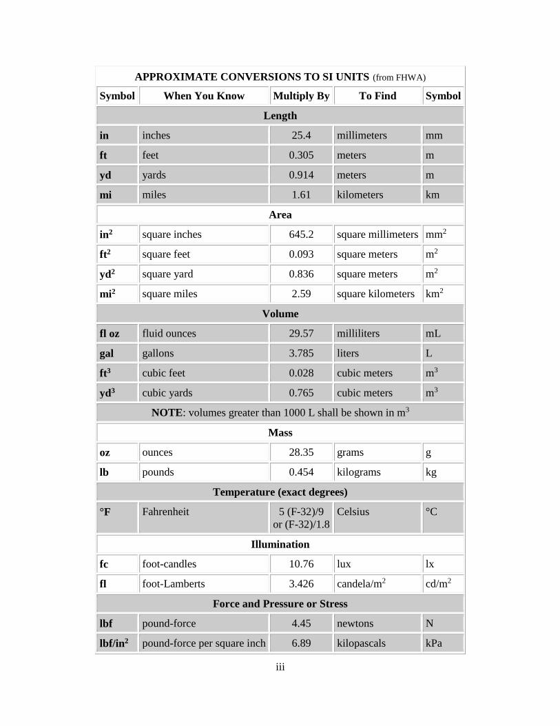
APPROXIMATE CONVERSIONS TO SI UNITS (from FHWA)

Symbol When You Know Multiply By To Find Symbol

Length

in inches 25.4 millimeters mm

ft feet 0.305 meters m

yd yards 0.914 meters m

mi miles 1.61 kilometers km

Area

in2 square inches 645.2 square millimeters mm2

ft2 square feet 0.093 square meters m2

yd2 square yard 0.836 square meters m2

mi2 square miles 2.59 square kilometers km2

Volume

fl oz fluid ounces 29.57 milliliters mL

gal gallons 3.785 liters L

ft3 cubic feet 0.028 cubic meters m3

yd3 cubic yards 0.765 cubic meters m3

NOTE: volumes greater than 1000 L shall be shown in m3

Mass

oz ounces 28.35 grams g

lb pounds 0.454 kilograms kg

Temperature (exact degrees)

°F Fahrenheit 5 (F-32)/9

or (F-32)/1.8

Celsius °C

Illumination

fc foot-candles 10.76 lux lx

fl foot-Lamberts 3.426 candela/m2 cd/m2

Force and Pressure or Stress

lbf pound-force 4.45 newtons N

lbf/in2 pound-force per square inch 6.89 kilopascals kPa

iv

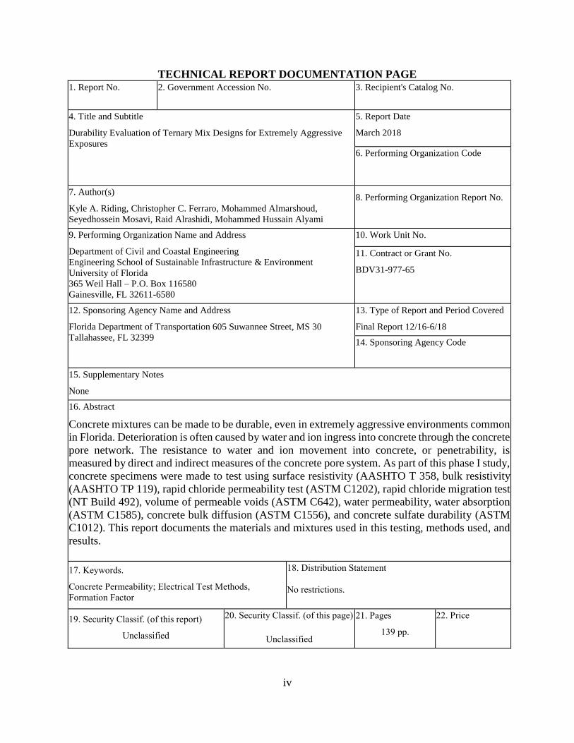
TECHNICAL REPORT DOCUMENTATION PAGE 1. Report No. 2. Government Accession No. 3. Recipient's Catalog No.

4. Title and Subtitle

Durability Evaluation of Ternary Mix Designs for Extremely Aggressive

Exposures

5. Report Date

March 2018

6. Performing Organization Code

7. Author(s)

Kyle A. Riding, Christopher C. Ferraro, Mohammed Almarshoud,

Seyedhossein Mosavi, Raid Alrashidi, Mohammed Hussain Alyami

8. Performing Organization Report No.

9. Performing Organization Name and Address

Department of Civil and Coastal Engineering

Engineering School of Sustainable Infrastructure & Environment

University of Florida

365 Weil Hall – P.O. Box 116580

Gainesville, FL 32611-6580

10. Work Unit No.

11. Contract or Grant No.

BDV31-977-65

12. Sponsoring Agency Name and Address

Florida Department of Transportation 605 Suwannee Street, MS 30

Tallahassee, FL 32399

13. Type of Report and Period Covered

Final Report 12/16-6/18

14. Sponsoring Agency Code

15. Supplementary Notes

None

16. Abstract

Concrete mixtures can be made to be durable, even in extremely aggressive environments common

in Florida. Deterioration is often caused by water and ion ingress into concrete through the concrete

pore network. The resistance to water and ion movement into concrete, or penetrability, is

measured by direct and indirect measures of the concrete pore system. As part of this phase I study,

concrete specimens were made to test using surface resistivity (AASHTO T 358, bulk resistivity

(AASHTO TP 119), rapid chloride permeability test (ASTM C1202), rapid chloride migration test

(NT Build 492), volume of permeable voids (ASTM C642), water permeability, water absorption

(ASTM C1585), concrete bulk diffusion (ASTM C1556), and concrete sulfate durability (ASTM

C1012). This report documents the materials and mixtures used in this testing, methods used, and

results.

17. Keywords.

Concrete Permeability; Electrical Test Methods,

Formation Factor

18. Distribution Statement

No restrictions.

19. Security Classif. (of this report)

Unclassified

20. Security Classif. (of this page)

Unclassified

21. Pages

139 pp.

22. Price

v

ACKNOWLEDGMENTS

The Florida Department of Transportation (FDOT) is acknowledged for funding this project. The

assistance of Dr. H.D. DeFord, Michael Bergin, Jose Armenteros, Ron Simmons, Teresa Risher,

and David Hudson is gratefully acknowledged.

vi

EXECUTIVE SUMMARY

Background

The Florida Department of Transportation (FDOT) currently uses the surface resistivity (SR) test

AASHTO T358 [1] as a standard test method for concrete mixture durability in aggressive chloride

environments. SR measures the concrete’s electrical resistance as an indicator of pore network

size, connectivity, and tortuosity. Previous testing by FDOT gave concern that this test may not

adequately measure concrete’s resistance to ion transport, especially for ternary-blend mixtures

that contain more than one type of supplementary cementitious material (SCM). Electrical

resistivity and chloride ion diffusivity are linked in theory by an empirical material parameter

called the formation factor, which is the ratio of the concrete diffusion coefficient to the free

chloride diffusion coefficient in the pore solution. It is also equal to the concrete electrical

conductivity divided by the electrical conductivity of the concrete pore solution. The formation

factor may normalize for pore solution differences in materials with the same ion penetrability and

allow for better comparisons of concrete mixtures.

Research Objectives

The research objective for this project was to find a correlation between concrete mixture

proportions for ternary blends and surface resistivity and other alternate concrete transport

property indexes. This phase I study aimed to make the concrete samples required for testing

concrete mixtures for resistance to water and ion ingress. Concrete testing at 28 and 56 days was

performed under this study.

Main Findings

The main findings from this study are summarized as follows:

Curing concrete samples in simulated pore solution greatly reduced the measured concrete

surface resistivity. Concrete curing method has a large effect on leaching and measured

resistivity results.

Correlations were found between surface resistivity and bulk resistivity, rapid chloride

permeability, concrete diffusivity measured by rapid chloride migration, and secondary

water absorption rate.

vii

Recommendations

Based on the correlations found so far in this study, FDOT should continue work to measure the

specimen properties at 1 year.

Future Work

Samples made under this phase I project to measure bulk diffusion after 6 and 12 months of

chloride exposure should be measured for chloride concentration with depth as part of a phase II

project. Samples made for the other transport property tests should also be measured at 12 months

in a phase II project. The ability of the formation factor to be normalized for differences between

material pore solution conductivities and improve correlation of electrical tests to other transport

property indexes should be explored in a phase II study.

viii

TABLE OF CONTENTS

DISCLAIMER ................................................................................................................................ ii

TECHNICAL REPORT DOCUMENTATION PAGE ................................................................. iv

ACKNOWLEDGMENTS .............................................................................................................. v

EXECUTIVE SUMMARY ........................................................................................................... vi

Background ................................................................................................................................ vi

Research Objectives ................................................................................................................... vi

Main Findings ............................................................................................................................ vi

Recommendations ..................................................................................................................... vii

Future Work .............................................................................................................................. vii

TABLE OF CONTENTS ............................................................................................................. viii

LIST OF TABLES ......................................................................................................................... xi

LIST OF FIGURES ..................................................................................................................... xiii

Chapter 1. Introduction ............................................................................................................ 1

1.1 Background ........................................................................................................................... 1

1.2 Research Objectives .............................................................................................................. 1

1.3 Research Approach ............................................................................................................... 1

Chapter 2. Literature Review .................................................................................................. 3

2.1 Introduction ........................................................................................................................... 3

2.2 Concrete Permeability and Transport Properties .................................................................. 4

2.3 Chloride Binding ................................................................................................................... 7

2.4 Permeability (Penetration Resistance) Test Methods ......................................................... 13

2.5 Supplementary Cementitious Materials .............................................................................. 34

Chapter 3. Concrete Mixture Design ..................................................................................... 39

ix

3.1 Type of Cement................................................................................................................... 39

3.2 Supplementary Cementitious Materials .............................................................................. 41

3.3 Aggregates .......................................................................................................................... 43

3.4 Chemical Admixtures ......................................................................................................... 43

Chapter 4. Materials Characterization ................................................................................... 45

4.1 Aggregate Properties ........................................................................................................... 45

4.2 Cementitious Materials ....................................................................................................... 46

Chapter 5. Specimen Fabrication for Transport and Electrical Property Testing ................. 50

5.1 Concrete Methodology........................................................................................................ 50

5.2 Electrical Tests .................................................................................................................... 56

Chapter 6. Fabricate Sample for Bulk Diffusion Testing ...................................................... 72

6.1 Introduction ......................................................................................................................... 72

6.2 Sample Preparation ............................................................................................................. 72

6.3 Epoxy Coating .................................................................................................................... 74

6.4 Calcium Hydroxide Bath .................................................................................................... 74

6.5 Exposure Condition ............................................................................................................ 74

Chapter 7. Chloride Binding Sample Fabrication ................................................................. 78

7.1 Cement Paste Mixtures ....................................................................................................... 78

7.2 Sample Preparation and Testing ......................................................................................... 80

Chapter 8. Sulfate Attack Specimen Fabrication .................................................................. 87

8.1 Introduction ......................................................................................................................... 87

8.2 Prism Preparation ................................................................................................................ 87

8.3 Modified ASTM C1012 ...................................................................................................... 90

8.4 Results to Date .................................................................................................................... 92

Chapter 9. Results.................................................................................................................. 94

x

9.1 Introduction ......................................................................................................................... 94

9.2 Compressive Strength ......................................................................................................... 94

9.3 Volume of Permeable Voids ............................................................................................... 97

9.4 Water Absorption ................................................................................................................ 99

9.5 Water Permeability ........................................................................................................... 101

9.6 Rapid Chloride Permeability Test ..................................................................................... 103

9.7 Rapid Chloride Migration Test (NT-Build 492) ............................................................... 105

9.8 Bulk (ASTM C1760) and Surface resistivity test (AASHTO T 358) ............................... 107

9.9 Discussion ......................................................................................................................... 110

9.9.2 Effect of Silica Fume ......................................................................................................... 113

9.9.3 Effect of Metakaolin .......................................................................................................... 118

9.9.4 Effect of Water-to-Cementitious Materials Ratio (W/CM) ............................................... 123

9.10 Comparison between Test Methods ................................................................................ 127

Chapter 10. Conclusions and recommendations ................................................................... 136

References ................................................................................................................................... 137

xi

LIST OF TABLES

Table 2-1: Sampling intervals for ponding test ASTM C1543 ..................................................... 15

Table 2-2: Applied voltage and duration of RCMT...................................................................... 17

Table 2-3: Advantages and disadvantages of common chloride diffusion tests ........................... 19

Table 2-4: Water absorption tests: advantage and disadvantages ................................................. 22

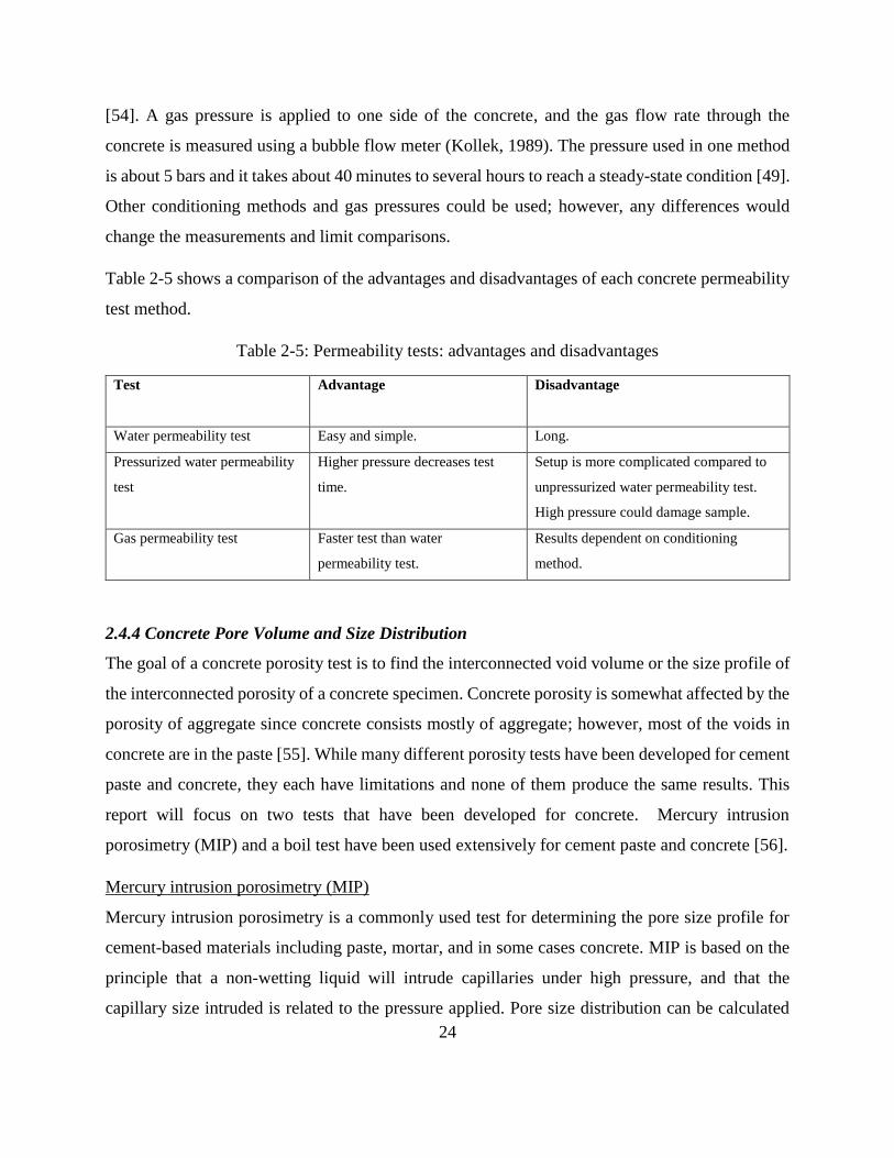
Table 2-5: Permeability tests: advantages and disadvantages ...................................................... 24

Table 2-6: Concrete pore volume and size distribution tests: advantages and disadvantages. ..... 28

Table 2-7: Chloride ion permeability classification [2] ................................................................ 31

Table 2-8: Self-diffusion coefficient of ionic species [66] ........................................................... 33

Table 3-1: Concrete mixture proportions ...................................................................................... 39

Table 4-1: Coarse aggregate specific gravity and absorption ....................................................... 45

Table 4-2: Coarse aggregate particle size distribution .................................................................. 45

Table 4-3: Fine aggregate specific gravity and absorption ........................................................... 46

Table 4-4: Fine aggregate particle size distribution ...................................................................... 46

Table 4-5: CCRL samples used to validate XRF calibration ........................................................ 47

Table 4-6: Cement and supplementary cementitious material composition as measured by XRF

....................................................................................................................................................... 48

Table 4-7: Cement composition analyzed by X-Ray diffraction and rietveld refinement ............ 49

Table 5-1: Measured concrete plastic properties .......................................................................... 53

Table 6-1: Mixing date and testing dates for the samples at different times ................................ 76

Table 7-1: Cement Paste Mixture Proportions.............................................................................. 78

Table 7-2: Chloride solution volume used during autotitration .................................................... 85

Table 8-1: Preliminary length change readings for concrete prisms exposed to 5% sodium sulfate

solution .......................................................................................................................................... 92

Table 9-1: Compressive strength of the mixtures at 28 days ........................................................ 94

Table 9-2: Volume of permeable voids for concrete mixtures at 28 days and 56 days of age ..... 98

Table 9-3: Absorption rate for 28 and 56 days ........................................................................... 100

Table 9-4: Permeability results ................................................................................................... 101

Table 9-5: Rapid chloride permeability test results at 28 and 56 days ....................................... 104

Table 9-6: RCMT at 28 and 56 days ........................................................................................... 105

Table 9-7: Surface and bulk resistivity measurements for SPS curing ....................................... 107

xii

Table 9-8: Surface and bulk resistivity measurements for moist room curing ........................... 109

xiii

LIST OF FIGURES

Figure 2-1: Chloride ponding test. ................................................................................................ 15

Figure 2-2: Rapid chloride migration test setup. .......................................................................... 17

Figure 2-3: RCMT concrete specimen split open showing area near surface with elevated

chloride levels stained by silver nitrate solution ........................................................................... 18

Figure 2-4: The concrete cover absorption test (CAT) setup. ...................................................... 21

Figure 2-5: The initial surface absorption test (ISAT) setup. ....................................................... 22

Figure 2-6: The difference between an actual and assumed pore shape. ...................................... 26

Figure 2-7: Four-point Wenner array probe test setup used in the SR test. .................................. 29

Figure 2-8: BR concrete specimen setup. ..................................................................................... 30

Figure 5-1: Determination of slump ............................................................................................. 51

Figure 5-2: Determination of unit weight ..................................................................................... 51

Figure 5-3: Determination of air content ...................................................................................... 52

Figure 5-4: Concrete temperature measurement ........................................................................... 53

Figure 5-5: Cylinders after being filled with the first layer of concrete ....................................... 55

Figure 5-6: Concrete prism mold after first layer of concrete added ............................................ 55

Figure 5-7: Surface resistivity meter used in this study ................................................................ 56

Figure 5-8: Specimen holder used in this study ............................................................................ 57

Figure 5-9: Surface resistivity measurement ................................................................................ 58

Figure 5-10: Grinding samples for bulk resistivity measurement ................................................ 59

Figure 5-11: Bulk resistivity test................................................................................................... 59

Figure 5-12: RCPT samples during testing ................................................................................... 61

Figure 5-13: RCMT during testing ............................................................................................... 62

Figure 5-14: Split surface of the specimen sprayed with silver nitrate ......................................... 63

Figure 5-15: Test specimen selection from different cylinders .................................................... 64

Figure 5-16: Water permeability specimen placed in the center of mold ..................................... 65

Figure 5-17: Schematic view of pouring epoxy ............................................................................ 66

Figure 5-18: Test specimen prepared to run the test ..................................................................... 67

Figure 5-19: Water permeability apparatus .................................................................................. 68

Figure 5-20: Immersion of sample in water .................................................................................. 69

Figure 5-21: Schematic of the water absorption procedure .......................................................... 70

xiv

Figure 5-22: Measuring sample weight at the specific time intervals .......................................... 70

Figure 6-1: Schematic view of the test specimen and reference sample obtained from the cylinder

....................................................................................................................................................... 73

Figure 6-2: Bulk diffusion samples during storage at 23±2ºC and 50% RH ................................ 74

Figure 6-3: Tank containing 16.5% NaCl solution and bulk diffusion samples ........................... 75

Figure 6-4: One-dimensional chloride ingress in the tank ............................................................ 75

Figure 7-1: High shear cement paste mixer .................................................................................. 80

Figure 7-2: Water bath to control the paste temperature. ............................................................. 81

Figure 7-3: Cement paste mixed with cooling base and feeder lid ............................................... 82

Figure 7-4: Paste rotator................................................................................................................ 82

Figure 7-5: Wavering saw used in cutting the cement paste disks ............................................... 83

Figure 7-6: Paste samples placed in chloride solution .................................................................. 84

Figure 7-7: Paste in chloride solution samples for all 38 mixtures............................................... 84

Figure 7-8: Autotitrator and the titrant.......................................................................................... 86

Figure 8-1: Prism molds assembled and ready for use ................................................................. 87

Figure 8-2: Concrete placement in mold ...................................................................................... 88

Figure 8-3: Prism being finished................................................................................................... 88

Figure 8-4: Sample after finishing ................................................................................................ 89

Figure 8-5: Prism demolding after initial curing .......................................................................... 89

Figure 8-6: Samples placed in moist curing room for curing prior to sulfate exposure ............... 90

Figure 8-7: Concrete prism in length comparator ......................................................................... 91

Figure 8-8: Prisms stored in 5% sodium sulfate solution ............................................................. 92

Figure 9-1: Water/cement ratio vs. compressive strength at 28 days ........................................... 96

Figure 9-2: Effect of metakaolin on concrete compressive strength (ASTM C39) at 28 days ..... 97

Figure 9-3: Water/cement ratio vs. volume of permeable voids at 28 days ................................. 99

Figure 9-4: Water permeability vs. w/cm ................................................................................... 103

Figure 9-5: Secondary absorption rate (ASTM C1585) vs Slag replacement at 28 days. Samples

contained Type I/II cement and 10% fly ash, with a w/cm of 0.35. ........................................... 111

Figure 9-6: Rapid chloride permeability (ASTM C1202) vs slag replacement at 28 days.

Samples contained Type I/II cement and 10% fly ash, with a w/cm of 0.35. ............................. 111

xv

Figure 9-7: Rapid chloride migration (NT Build 492) vs slag replacement at 28 days. Samples


Figure 9-8: Surface resistivity (AASHTO T 358) vs slag replacement at different ages (Moist

room). Samples contained Type I/II cement and 10% fly ash, with a w/cm of 0.35. ................ 112

Figure 9-9: Surface resistivity (AASHTO T 358) vs slag replacement at different ages (SPS).


Figure 9-10: Compressive strength (ASTM C39) vs. silica fume replacement at 28 days.


Figure 9-11: Volume of permeable voids (ASTM C642) vs silica fume replacement at 28 days.


Figure 9-12: Secondary absorption rate (ASTM C1585) vs silica fume replacement at 28 days.


Figure 9-13: Rapid chloride permeability (ASTM C1202) vs. silica fume replacement at 28 days.


Figure 9-14: Rapid chloride migration (NT Build 492) vs. silica fume replacement at 28 days.


Figure 9-15: Surface resistivity (AASHTO T358) vs silica fume replacement at different ages

(Moist room). Samples contained Type I/II cement and 20% fly ash, with a w/cm of 0.35. .... 117

Figure 9-16: Bulk resistivity (ASTM C1760) vs silica fume replacement at different ages (Moist


Figure 9-17: Bulk resistivity (ASTM C1760) vs silica fume replacement at different ages (SPS).


Figure 9-18: Compressive strength (ASTM C39) vs metakaolin replacement at 28 days. Samples


Figure 9-19: Secondary absorption rate (ASTM C1585) vs metakaolin replacement at 28 days.


Figure 9-20: Rapid chloride permeability (ASTM C1202) vs metakaolin replacement at 28 days.


Figure 9-21: Rapid chloride migration (NT Build 492) vs metakaolin replacement at 28 days.


xvi

Figure 9-22: Surface resistivity (AASHTO T 358) vs metakaolin replacement at different ages

(moist room). Samples contained Type I/II cement and 20% fly ash, with a w/cm of 0.35...... 122


(SPS). Samples contained Type I/II cement and 20% fly ash, with a w/cm of 0.35. ................ 122

Figure 9-24: Bulk resistivity (ASTM C1760) vs. metakaolin replacement at different ages (Moist


Figure 9-25: Compressive strength (ASTM C39) vs. fly ash replacement and w/cm ratio at 28

days. Samples contained Type I/II cement. ............................................................................... 124

Figure 9-26: Volume of permeable voids (ASTM C642) vs. fly ash and w/cm ratio replacement

at 28 days. Samples contained Type I/II cement. ...................................................................... 124

Figure 9-27: Secondary absorption rate ASTM C1585) vs. fly ash replacement and w/cm ratio at

28 days. Samples contained Type I/II cement. .......................................................................... 125

Figure 9-28: Rapid chloride permeability (ASTM C1202) vs. fly ash and w/cm ratio replacement

at 28 days. Samples contained Type I/II cement. ...................................................................... 126

Figure 9-29: Rapid chloride migration (NT Build 492) vs. fly ash replacement and w/cm ratio at

28 days. Samples contained Type I/II cement. .......................................................................... 126

Figure 9-30: Compressive strength vs. volume of permeable voids at 28 days ......................... 127

Figure 9-31: Compressive strength vs. secondary absorption at 28 days ................................... 128

Figure 9-32: Water permeability vs. secondary absorption rate at 28 days ................................ 129

Figure 9-33: Water permeability vs rapid chloride permeability (ASTM C1202) at 28 days .... 130

Figure 9-34: Initial and secondary absorption rate for each mix group ...................................... 131

Figure 9-35: RCMT vs. RCPT at 28 days .................................................................................. 132

Figure 9-36: RCPT (ASTM C1202) vs. surface resistivity (SR, AASHTO T 358)) at 28 days. SR

samples were cured in the moist room with one group exposed to the moist air (blue) and the

other stored in SPS in closed containers (red). ........................................................................... 133

Figure 9-37: Bulk resistivity vs. secondary absorption rate at 28 days ...................................... 134

Figure 9-38: Surface resistivity vs. bulk resistivity at 28 days ................................................... 135

CHAPTER 1. INTRODUCTION

1.1 Background


AASHTO T358 [1] as the standard test method for concrete mixture durability in aggressive

chloride environments. SR measures the concrete’s electrical resistance as an indicator of the

concrete pore network size, connectivity, and tortuosity. Chlorides and other aggressive ions,

which can cause reinforcement corrosion or other concrete deterioration, penetrate into the

concrete through the pore network. A reduction in the concrete pore network connectivity and

increase in tortuosity reduce the chloride ingress rate and increase durability. Reductions in the

concrete pore network permeability should be reflected by an increase in the SR. Previous testing

by FDOT gave concern that this test may not adequately measure concrete’s resistance to ion

transport, especially for ternary-blend mixtures that contain more than one type of supplementary

cementitious material (SCM). Electrical resistivity and chloride ion diffusivity are linked in theory

by an empirical material parameter called the formation factor, which is the ratio of the concrete

diffusion coefficient to the free chloride diffusion coefficient in the pore solution. It is also equal

to the concrete electrical conductivity divided by the electrical conductivity of the concrete pore

solution. The formation factor is considered a material property in that it normalizes the effect of

pore solution chemistry (conductivity), giving a measure of the ionic penetrability of the concrete.

1.2 Research Objectives

This is Phase I of a project with a primary objective to determine which test methods best indicate

the aqueous intrusion resistance for representative classes of concrete and ternary combinations of

cementitious materials. This work also examined whether use of the formation factor can mitigate

the effect of pore solution concentration on concrete electrical properties. Another important

objective was to select ternary concrete mix designs for long-term durability testing.

1.3 Research Approach

The research approach used consisted of performing a literature review covering concrete ion

penetrability, the effect of mixture proportions on concrete ion penetrability, and test methods to

2

measure the concrete resistance to ion penetrability. Specimens for the following electrical tests

were made as an indirect measure of concrete transport properties:

Surface resistivity (AASHTO T 358)

Bulk resistivity (AASHTO TP 119) [2]

Rapid Chloride Permeability Test (ASTM C1202) [3]

Specimens for the following tests related to concrete transport properties were made:

Rapid Chloride Migration Test (NT Build 492) [4]

Water Permeability

Concrete Water Absorption Rate (ASTM C1585)

Concrete Pore System Using Mercury Intrusion Porosimetry. Procedures developed

during the FDOT project “Evaluation of Porometry, Permeability and Transport of

Structural Concrete” BDV31-977-42 performed at UF will be followed after samples

have reached the appropriate age.

Concrete volume of permeable voids (ASTM C642)

Samples to measure the concrete chloride bulk diffusivity were made. Samples to measure the

cementitious material chloride binding isotherms were made to separate the chloride binding from

chloride diffusion in the concrete bulk diffusion testing (ASTM C1556). Concrete samples for

sulfate durability were also made for comparison. Test results to date are presented in this Phase I

repot, with final results of all testing presented in the Phase II final report.

3

CHAPTER 2. LITERATURE REVIEW

2.1 Introduction


AASHTO T358 [1] as a standard test method for concrete mixture durability in aggressive

chloride-containing environments. SR measures the concrete’s electrical resistance as an indicator

of the concrete pore network size, connectivity, and tortuosity. Chlorides and other aggressive ions

that can cause reinforcement corrosion or other concrete deterioration enter into the concrete

through the pore network. Reduction in the concrete pore network connectivity and increase in

tortuosity reduce the chloride ingress rate and increase durability. Reductions in the concrete pore

network permeability typically increase SR.

Electrical resistivity and chloride ion diffusivity are linked by the formation factor, which is the

ratio of the concrete diffusion coefficient to that of the free chloride diffusion coefficient in the

pore solution [5]. Formation factor is likewise equal to the concrete electrical conductivity divided

by the electrical conductivity of the concrete pore solution. In theory, if the concrete pore solution

conductivity and chloride free diffusion coefficient are known, and the electrical resistivity is

measured, the concrete diffusion coefficient can be calculated [5,6]. There are three methods for

estimating the pore solution conductivity: measure the conductivity using a simple sensor, extract

the pore solution through high pressure, or estimate the pore solution conductivity using the cement

composition and an online calculator [7]. A past attempt at correlating the chloride diffusion with

the surface resistivity failed most likely because the measurements did not account for chloride

binding [5]. Accounting for chloride binding could improve the measured correlation between the

formation factor and chloride diffusion coefficient.

Ternary mixtures that combine more than one supplementary cementitious material (SCM) in

concrete and low water-to-cementitious material ratio (w/cm) have been promoted by FDOT as a

cost-effective means to reduce concrete permeability. Recent FDOT results, however, have shown

that for ternary mixtures, expected relationships between SR and silica fume content or w/cm were

not found [8]. Other factors that influence the concrete electrical resistivity, such as pore solution

conductivity, temperature, and specimen surface drying could affect results [6]. For samples that

are well cured and do not have temperature or surface drying effects, the formation factor could

4

account for the effect of differences in pore solution conductivity on the concrete electrical

resistivity. It is possible that other available tests that measure concrete properties related to

transport, besides electrical resistivity tests, could correlate with performance. These test methods

include mercury intrusion porosimetry, water absorption (ASTM C1585) [9], water permeability,

and bulk diffusion (ASTM C1556) [10].

SR has been used as a gauge of the concrete performance in aggressive chloride environments.

Very little work has been done though to determine if SR can be used as an index of the concrete

performance in sulfate environments. Sulfate attack can occur in two different ways: degradation

through chemical reactions and breakdown of the concrete or salt weathering. Both mechanisms

require sulfate ions to be transported through the concrete pore system in order to cause damage

[9]. In chemical sulfate attack, sulfate ions react with calcium hydroxide located in the pore

solution to produce gypsum. The products further react with un-hydrated C3A causing the

formation of ettringite and monosulfate. The formation of gypsum and ettringite will cause an

increase in volume of 1.2 and 2.5 times, respectively. Physical salt attack occurs when salts in the

pores undergo an expansive phase change. This can occur with sodium sulfate salts that can convert

from thenardite (Na2SO4) to mirabilite (Na2SO4·10H2O) during diurnal temperature changes. This

phase change causes a 4 to 5 times increase in volume [11]. These chemical reactions and the

crystallization of salts will cause internal stresses in the concrete structure due to expansion, which

causes reduction in strength due to cracking, spalling, and deterioration [12]. An increase in the

concrete surface resistivity could correlate well with improvements in sulfate attack resistance

because concrete with lower permeability could keep sulfate ions out of the concrete.

2.2 Concrete Permeability and Transport Properties

2.2.1 Transport Properties

Transport property tests can provide an indication of the ability of concrete to prevent water and

ion ingress into concrete since transport of water and ions occurs in the concrete pore network.

Concrete transport property tests either directly measure water or ion transport or indirectly

measure properties controlled by the pore system. Because all transport property tests relate to the

pore system, for a given cementitious system, there are correlations between transport properties

5

results. Water and its associated ions can enter the concrete through five principal mechanisms:

diffusion, electromigration, thermal migration, absorption, and pressure [13,14]. All of these

mechanisms occur because of a driving force based on a driving gradient. Diffusion, absorption,

and pressure-based mechanisms are responsible for a majority of chloride ingress in most concrete

structures.

Diffusion is driven by a concentration gradient and can be described as the movement of an ion

without any fluid flow. Solutions with different concentrations tend toward the same concentration

when put in contact with each other. For example, putting salt in water will cause the salt to

dissolve, and through a diffusion process, to assume a uniform concentration. Similarly, ions that

are present in the concrete pore solution will redistribute, due to the concentration gradients, until

there is an equal concentration throughout the sample. Fick’s second law of diffusion can be used

to model mass transport through diffusion in saturated concrete according to Equation 2-1 [15]:

2

2

dx

CdD

dt

dC

Equation 2-1

where, C is the concentration (%), t is time (s), x is distance (m), and D is the diffusion coefficient

(m2/s). The diffusion coefficient is dependent on the ion of interest, the concrete pore size

distribution and total porosity, and the pore connectivity [16]. Equation 1 can be simplified

assuming a constant diffusion coefficient with time and location, a constant surface concentration,

no chloride binding, and using the error function, as shown in Equation 2-2 [17]:

𝐶 = 𝐶𝑠(1 − erf (𝑥

2√𝐷𝑡))

Equation 2-2

where CS is the surface chloride content (mass percentage), and t is the exposure duration.

Pressure differentials may be created by external water pressure in some types of structures, such

as dams and tunnel lining. As the water flows through concrete, it will typically bring with it

dissolved ions that can deteriorate the concrete or embedded reinforcing steel [15]. The concrete

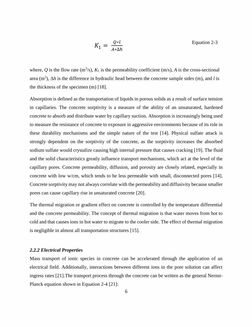
permeability coefficient K1 can be calculated using Darcy’s law as shown in Equation 2-3 [18]:

6

𝐾1 = 𝑄∗𝑙

𝐴∗∆ℎ

Equation 2-3

where, Q is the flow rate (m3/s), K1 is the permeability coefficient (m/s), A is the cross-sectional

area (m2), Δh is the difference in hydraulic head between the concrete sample sides (m), and l is

the thickness of the specimen (m) [18].

Absorption is defined as the transportation of liquids in porous solids as a result of surface tension

in capillaries. The concrete sorptivity is a measure of the ability of an unsaturated, hardened

concrete to absorb and distribute water by capillary suction. Absorption is increasingly being used

to measure the resistance of concrete to exposure in aggressive environments because of its role in

these durability mechanisms and the simple nature of the test [14]. Physical sulfate attack is

strongly dependent on the sorptivity of the concrete, as the sorptivity increases the absorbed

sodium sulfate would crystalize causing high internal pressure that causes cracking [19]. The fluid

and the solid characteristics greatly influence transport mechanisms, which act at the level of the

capillary pores. Concrete permeability, diffusion, and porosity are closely related, especially in

concrete with low w/cm, which tends to be less permeable with small, disconnected pores [14].

Concrete sorptivity may not always correlate with the permeability and diffusivity because smaller

pores can cause capillary rise in unsaturated concrete [20].

The thermal migration or gradient effect on concrete is controlled by the temperature differential

and the concrete permeability. The concept of thermal migration is that water moves from hot to

cold and that causes ions in hot water to migrate to the cooler side. The effect of thermal migration

is negligible in almost all transportation structures [15].

2.2.2 Electrical Properties

Mass transport of ionic species in concrete can be accelerated through the application of an

electrical field. Additionally, interactions between different ions in the pore solution can affect

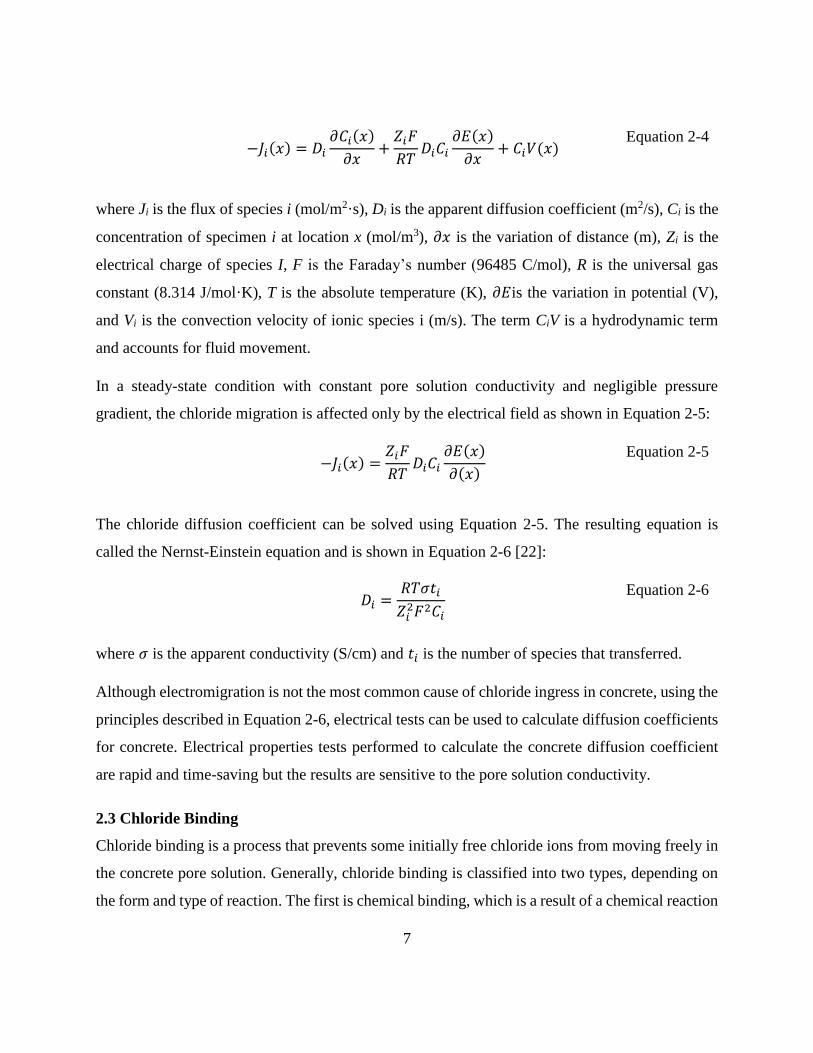
ingress rates [21].The transport process through the concrete can be written as the general Nernst-

Planck equation shown in Equation 2-4 [21]:

7

−𝐽𝑖(𝑥) = 𝐷𝑖

𝜕𝐶𝑖(𝑥)

𝜕𝑥+

𝑍𝑖𝐹

𝑅𝑇𝐷𝑖𝐶𝑖

𝜕𝐸(𝑥)

𝜕𝑥+ 𝐶𝑖𝑉(𝑥)

Equation 2-4

where Ji is the flux of species i (mol/m2·s), Di is the apparent diffusion coefficient (m2/s), Ci is the

concentration of specimen i at location x (mol/m3), 𝜕𝑥 is the variation of distance (m), Zi is the

electrical charge of species I, F is the Faraday’s number (96485 C/mol), R is the universal gas

constant (8.314 J/mol·K), T is the absolute temperature (K), 𝜕𝐸is the variation in potential (V),

and Vi is the convection velocity of ionic species i (m/s). The term CiV is a hydrodynamic term

and accounts for fluid movement.

In a steady-state condition with constant pore solution conductivity and negligible pressure

gradient, the chloride migration is affected only by the electrical field as shown in Equation 2-5:

−𝐽𝑖(𝑥) =

𝑍𝑖𝐹

𝑅𝑇𝐷𝑖𝐶𝑖

𝜕𝐸(𝑥)

𝜕(𝑥)

Equation 2-5

The chloride diffusion coefficient can be solved using Equation 2-5. The resulting equation is

called the Nernst-Einstein equation and is shown in Equation 2-6 [22]:

𝐷𝑖 =

𝑅𝑇𝜎𝑡𝑖

𝑍𝑖2𝐹2𝐶𝑖

Equation 2-6

where 𝜎 is the apparent conductivity (S/cm) and 𝑡𝑖 is the number of species that transferred.

Although electromigration is not the most common cause of chloride ingress in concrete, using the

principles described in Equation 2-6, electrical tests can be used to calculate diffusion coefficients

for concrete. Electrical properties tests performed to calculate the concrete diffusion coefficient

are rapid and time-saving but the results are sensitive to the pore solution conductivity.

2.3 Chloride Binding

Chloride binding is a process that prevents some initially free chloride ions from moving freely in

the concrete pore solution. Generally, chloride binding is classified into two types, depending on

the form and type of reaction. The first is chemical binding, which is a result of a chemical reaction

8

between chloride ions and un-hydrated cementitious material or hydrated product. The second is

physical binding, which is holding the chloride ions by adsorption in the calcium silicate hydrate

(C-S-H) gel. Note: in cement chemistry notation, C = CaO, S = SiO2 $ = SO3, F = Fe2O3, A =

Al2O3, and H = H2O [23].

2.3.1 Chemical Bonding

Chemical binding is a result of chemical reaction between free chloride ions in pore solution and

un-hydrated cement and cement hydration products. The chloride chemical binding is the main

factor dominating free chloride ion binding in concrete, and it is highly dependent on unhydrated

C3A content. C4AF also contributes to free chloride binding [24]. Friedel’s salt (C3F.CaCl2.10H2O)

forms as a result of the reaction of C3A and C4AF with the free chloride ions in the concrete pore

solution. Chemical bonding of chloride is, however, strongly affected by the presence of sulfate

ions in the pore solution. Free sulfates react with the un-hydrated C3A, which reduces the chemical

binding of free chloride ions [23]. Ettringite is formed until all the sulfate is consumed during the

hydration process of portland cement, after that the formation of Friedel’s salt binds free chlorides

[25]. The free chloride binding results from the direct chemical reaction between the C3A phase in

the portland cement and CaCl2 leading to the formation of Kuzel’s and Friedel’s salts as shown in

Equation 2-7, Equation 2-8 and Equation 2-9 [26]:

Ca(OH)2 + 2NaCl ↔ CaCl2 + 2Na- + 2OH- Equation 2-7

C3A + ½ CaCl2 + ½ CaSO4 + 10H2O →

C3A·½CaSO4·½CaCl2·10H2O

Equation 2-8

C3A + CaCl2 + 10H2O → C3A·CaCl2·10H2O Equation 2-9

The negative effect of sulfate on free chloride ion binding is dominant at low chloride

concentrations (0.1 M). The reaction of sulfates with C3A and C4AF results in the formation of

ettringite or monosulfate. As the free chloride ion concentration increases, the monosulfate

transforms into Kuzel’s salt first, and then into Friedel’s salt. Ettringite also starts to react to form

Friedel’s salt at higher concentrations of chlorides (≥3.0 M) [23].

9

Hydroxyl ions in the AFm (Al2O3-Fe2O3-monosulfate) interlayers can be replaced with free

chloride ions through an ion exchange mechanism, as shown in Equation 2-10. This ion exchange

mechanism leads to the formation of Friedel’s salt from AFm phases [27]:

R- OH-+ Na+ + Cl- → R-Cl- + Na+ + OH- Equation 2-10

where R is the principal layer of the hydroxy-AFm [Ca2Al(OH-)6·nH2O]-, where the value of n is

related to the type of hydoxy-AFm.

2.3.2 Physical Binding

Chloride physical binding is a result of free chloride ions entrapped in C-S-H gel. This process is

highly dependent on the formation of C-S-H gel. Physical binding is mainly controlled by the

adsorption of free chloride ions by the C-S-H gel. Binding is not only influenced by the quantity

of C-S-H, but also by the calcia-to-silica ratio (C/S). Lower C/S causes a reduction in the chloride

binding capacity of C-S-H gel [24].

C-S-H hydrates adsorb chloride ions onto their surface by electrostatic or van der Waals forces

between charged particles. The surfaces of the hydrated cement are negatively charged, but due to

the adsorption of cations (Ca2+, Na+) in the alkaline pore solution and the formation of the so-

called Stem-layer, the surfaces appear to be positively charged. This leads to the formation of an

electrical, diffuse double layer (known as the Gouy-Chapman layer), and the adsorption of the

negatively-charged chloride ions takes place in the diffuse double layer to satisfy the electro-

neutrality [28].

The surface area of the C-S-H gel is considered the main factor influencing the adsorption capacity

in the double layer. The zeta potential is a measure of the surface charge potential. The valence of

the adsorbed cations, temperature, and the concentration in the pore solution all affect the zeta

potential [23].

10

2.3.3 Effect of Chloride Binding on Chloride Migration

Fick’s second law can adequately describe chloride diffusion in concrete in submerged

environments [24]. In cases where chloride binding is present, the bound chloride ion will be

removed from the diffusion flux and can be subtracted from the conservation of mass equation as

shown in Equation 2-11 and Equation 2-12 [24]:

ct = cb + cf ωe Equation 2-11

𝜔𝑒

𝜕𝑐𝑓

𝜕𝑡=

𝜕

𝜕𝑥𝐷𝑒 × 𝜔𝑒

𝜕𝑐𝑓

𝜕𝑥−

𝜕𝑐𝑏

𝜕𝑡

Equation 2-12

where cf is the free chloride concentration (kg/m3) in the pore solution, cb is the bound chloride

concentration (kg/m3) in the concrete, ct is the total chloride concentration (kg/m3) in the concrete,

De is the effective diffusion coefficient and ωe is the evaporable water content (m3 solution/m3

concrete).

2.3.4 Chloride Binding Isotherm

The chloride binding isotherm is defined as the relationship between free and bound chloride ions

over a range of chloride concentrations at a given temperature. Tuutti proposed in 1982 the first

mathematical relationship to approximate the relationship between free and bound chloride

concentrations, which was a linear binding isotherm. Langmuir and Freundlich isotherms have

also been proposed to describe chloride binding [29].

1) Linear binding isotherm

The linear binding isotherm is described by Equation 2-13:

Cb = kCf Equation 2-13

11

where Cb is the concentration of bound chlorides, k is a unitless constant, and Cf is the concentration

of free chlorides. The linear binding isotherm approximates well the actual free and bound chloride

concentration relationship for free chloride concentrations lower than 20 g/l, but not above. The

actual free and bound chloride concentration relationship is too nonlinear to be well approximated

by a linear mathematical relationship for the range of free chloride concentrations found in

concrete. The linear binding isotherm is not recommended for use in concrete applications [30].

2) Langmuir binding isotherm

The Langmuir isotherm assumes monolayer adsorption. The slope of a plot of the isotherm curve

at high concentrations approaches zero, as indicated from Equation 2-14:

Cb =

𝛼 𝐶𝑓

(1+𝛽 𝐶𝑓) Equation 2-14

where α and β are unitless coefficients that depend on the compositions of the cementitious

materials. These coefficients are obtained by nonlinear curve-fitting of experimental data. The

Langmuir isotherm shows an excellent fit to measured data at concentrations lower than 0.05 M

(1.77 g/L) [31].

3) Freundlich binding isotherm

The Freundlich binding isotherm defines the relationship between bound and free chloride ions as

shown in Equation 2-15:

Cb = α Cf β Equation 2-15

where α and β are unitless coefficients.

The absorption of free chloride ions becomes more complicated in concentrations higher than 0.05

M, and the relationship between free and bound chlorides is described better by using the

Freundlich isotherm instead of Langmuir [31].

12

2.3.5 Factors Affecting Chloride Binding

The binding of free chloride ions with chemical components and hydration products of

cementitious materials is very complicated, and is influenced by many factors including chloride

concentration, cement composition, hydroxyl concentration, chloride salt cation, temperature,

SCM contents, carbonation, and sulfate concentration [32].

Portland cement type and composition

Numerous studies have shown that as the C3A content increases, the chloride binding capacity

increases [27]. The increase in chloride binding is due to the reactions between chloride ions and

C3A or C4AF, resulting in the formation of Friedel’s salt and its analogue [23]. Carbonation or

intruded sulfate could affect the chemically bound chloride and reverse the chloride chemical

bonding reactions [33]. The C3A content is considered a good indicator of the chloride binding

capacity of portland cement in high chloride concentrations (1.0–3.0 M), while it is a poor indicator

of chloride binding at low concentration (0.1 M). The chloride binding capacity of C4AF is about

one third of that of C3A [23].

C3S and C2S contents are the major components that control the formation of C-S-H as a product

of the portland cement hydration process. Since C-S-H adsorbs chloride ions, higher amounts of

C-S-H produced by the cement correspond with higher chloride binding [31]. The C/S ratio in the

C-S-H also affects chloride binding. Higher C/S ratios correspond with increased chloride binding

capacities [34]. Physical binding from C-S-H can account for 25 to 50% of the total binding

capacity [23].

Sulfate ions reduce chloride chemical binding due to their reaction with unhydrated C3A and C4AF

to form ettringite until all of the sulfate is consumed. After that, the free chloride ions react with

the remaining unhydrated C3A and C4AF to form Kuzel’s salt in low free chloride ion

concentration (0.1 M), and Friedel’s salt at higher concentration (3.0 M) [23,24].

13

pH

For a given total chloride content, the chloride binding increases with the decrease of hydroxyl ion

concentration. This is due to the competition between free chloride ions and hydroxyl ions for

adsorption sites on cement surfaces [35].

Water-to-cement ratio (w/c)

As the w/c ratio increases in a particular mixture, there is a proportional decrease in the chloride

concentration in the mix water. This might have been expected to cause a reduction in chloride

binding. However, chloride binding increases as w/c increases. This is probably due to the increase

in porosity and permeability of the higher w/c paste allowing greater access of chloride ions to the

cement particles [32]. Reducing the w/c could reduce the adsorption capacity of the C-S-H gel.

Temperature

Some studies show that at a low chloride concentration (<1.0 M), an increase in the temperature

will result in decreased free chloride ion binding. On the other hand, in high chloride

concentrations (~3.0 M), an increase in the temperature will cause an increase in free chloride ion

binding [23]. At higher temperatures, ettringite is less stable, favoring the decomposition of

ettringite and formation of Friedel’s salt [24].

Carbonation

Carbonation reacts with cement hydration products to form CaCO3, silica gel, and alumina gel.

During this process, concrete pH value will drop from 12.5 to around 9. The decomposition of C–

S–H due to the carbonation of calcium ions and the reduction in total porosity could cause

reduction in ion exchange and physical binding. Lower pH from carbonation greatly decreases

hydroxyl ion availability and increases the solubility of Friedel’s salt [36,37]. In general,

carbonation decreases the chemical binding capacity of cement-based materials, which causes

chlorides from Friedel’s salt to release into pore solution. This results in an increase in the pore

solution free chloride concentration.

2.4 Permeability (Penetration Resistance) Test Methods

Methods used to quantify the permeability of concrete attempt to determine the concrete’s

resistance to penetration by gases or liquids that can reduce the long-term durability. Multiple

14

methods are used to gage concrete’s penetrability to deleterious substances, many of which

correlate to one another [15]. The ability of fluids to transport through concrete depends on the

number and size of the pores and their connectivity [16]. The most common methods for assessing

concrete penetrability are discussed in the following sections.

2.4.1 Chloride Diffusion Testing

Chloride diffusion testing is used to quantify the concrete’s ability to resist chloride penetration

and assess the potential service life [38,39]. The traditional way to test chloride ion penetration is

by exposing the concrete sample to a chloride solution and measuring, for a given time of exposure,

the resulting chloride concentration as a function of depth from the ponded surface. Applying an

electrical voltage to accelerate the chloride ion penetration through concrete is also used in some

standardized test methods [24].

Chloride ponding test

The chloride ponding test is a standard test method for determining the penetration of chloride ion

into concrete by ponding as described in ASTM C1543 and AASHTO T259. The test exposes a

concrete specimen to a ponded 3% sodium chloride solution for a period of testing in a controlled

temperature and relative humidity as shown in Figure 2-1. A dike made out of mortar or other

means is used to contain the chloride solution on the concrete surface. A glass plate or polyethylene

sheet is also placed over the sample to reduce evaporation. The chloride penetration is determined

per depth and ponding duration [40]. The concrete chloride concentration with depth is typically

measured for the first time after 3 months of ponding. It can be re-measured after 6 months, 12

months of ponding, and annually thereafter. After ponding the concrete sample for the required

duration, concrete cores or powdered samples from a rotary impact hammer are taken according

to ASTM C1152 at different depths and measured for chloride content. The sample diameter for

cores shall be more than triple the nominal aggregate size used in the concrete mixture. Finally,

the chloride profile is found by testing at least four different depth intervals as indicated in Table

2-1 [40]. The chloride content is determined by using the ASTM C1152 acid-soluble chloride in

mortar and concrete testing method. The background chloride content measured from a companion

15

cylinder that was not exposed to chlorides is subtracted from the measured chloride content at each

depth to give the final chloride increase at each depth from ponding.

Figure 2-1: Chloride ponding test.

Table 2-1: Sampling intervals for ponding test ASTM C1543

Interval Interval depth (mm)

1 10 – 20

2 25 – 35

3 40 – 50

4 55 - 65

The chloride ponding test gives a reasonable estimate of the concrete resistance to chloride

penetration. The test does not provide any information on chloride binding. It is an expensive

16

and very time-consuming test that makes it difficult for widespread mixture qualification and

quality control testing.

Rapid chloride migration test (RCMT)

The rapid chloride migration test (RCMT, NT Build 492) uses electrical voltage to accelerate

chloride migration as shown in Figure 2-2. The test specimen shall be 4 inches in diameter and 2

inches thick, and prior testing the specimen is vacuum-impregnated with saturated lime solution

as described in NT Build 492 [4]. After the specimen is prepared, the concrete is exposed to a 10%

NaCl solution on one side and a 0.3 N NaOH solution on the other. The test starts by measuring

the initial current through the sample for an applied 30 volts. Based on the measured initial current,

the test duration and voltage for the remainder of the test are determined according to Table 2-2.

The initial and final current through the specimen and specimen temperature are measured. After

the test duration is completed, the concrete specimen is split open and a 0.1 M silver nitrate reagent

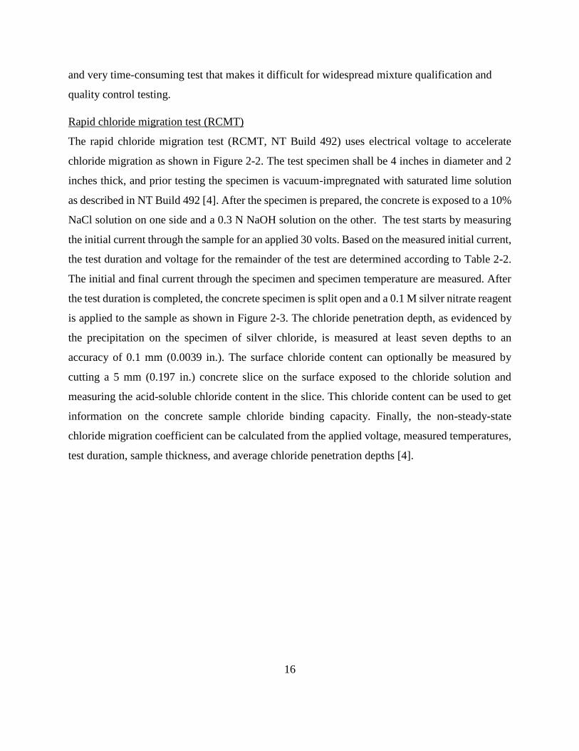
is applied to the sample as shown in Figure 2-3. The chloride penetration depth, as evidenced by

the precipitation on the specimen of silver chloride, is measured at least seven depths to an

accuracy of 0.1 mm (0.0039 in.). The surface chloride content can optionally be measured by

cutting a 5 mm (0.197 in.) concrete slice on the surface exposed to the chloride solution and

measuring the acid-soluble chloride content in the slice. This chloride content can be used to get

information on the concrete sample chloride binding capacity. Finally, the non-steady-state

chloride migration coefficient can be calculated from the applied voltage, measured temperatures,

test duration, sample thickness, and average chloride penetration depths [4].

17

Figure 2-2: Rapid chloride migration test setup.

Table 2-2: Applied voltage and duration of RCMT

Initial current (mA) Testing voltage (V) Possible new initial current (mA) Duration (h)

I30 < 5 60 I0 < 10 96

5 < I30 < 10 60 10 < I0 < 20 48

10 < I30 < 15 60 20 < I0 < 30 24

15 < I30 < 20 50 25 < I0 < 35 24

20 < I30 < 30 40 25 < I0 < 40 24

30 < I30 < 40 35 35 < I0 < 50 24

40 < I30 < 60 30 40 < I0 < 60 24

60 < I30 < 90 25 50 < I0 < 75 24

90 < I30 < 120 20 60 < I0 < 80 24

120 < I30 < 180 15 60 < I0 < 90 24

180 < I30 < 360 10 60 < I0 < 120 24

I30 > 360 10 I0 > 120 6

Rubber sleeve

18

Figure 2-3: RCMT concrete specimen split open showing area near surface with elevated

chloride levels stained by silver nitrate solution

This test method, while it is much more rapid than the chloride ponding test, has some drawbacks.

The electrical field can change the test and concrete properties. The concrete sample temperature,

mass, and resistivity have been shown to increase during the test. The NaCl solution pH increases

from hydroxyl ion migration, changing the OH-/Cl- ratio in the solution and the Cl- migration rate.

The sample saturation is also thought to increase during the test. This contradicts the test

assumption that the sample is saturated from the vacuum saturation process used to prepare the

samples. It was found that the calculated diffusion coefficient is about 10% higher for samples

tested at 60 V than those at 35 V, unless nonlinear chloride binding was accounted for in the

calculations [41].

Chloride bulk diffusion test

The chloride bulk diffusion test is described in ASTM C1556 [10]. In this test, a concrete core,

cylinder, or cube is divided into two parts. The top 3 inches of the sample is sealed from all sides,

except the finished surface, with epoxy and then vacuum-saturated with calcium hydroxide

solution. The bottom portion of the sample is used to measure the concrete initial chloride

concentration. After sealing the sides and bottom of the top specimen, it is submerged in sodium

19

chloride solution for at least 35 days. The chloride content with depth in the chloride-exposed

sample and the initial chloride content from the bottom sample are measured using titration as

specified in ASTM C1152 [10]. The chloride diffusion coefficient can then be calculated by fitting

a calculated chloride profile to the measured chloride profile. The main disadvantage of the test is

the time required to prepare and expose the sample to chlorides. Some studies have shown that

RCMT and Chloride bulk diffusion results show similar improvements in concrete chloride ingress

properties with the use of SCMs [42].

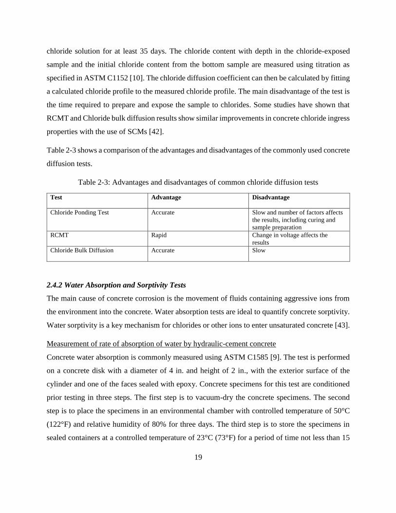
Table 2-3 shows a comparison of the advantages and disadvantages of the commonly used concrete

diffusion tests.

Table 2-3: Advantages and disadvantages of common chloride diffusion tests

Test

Advantage Disadvantage

Chloride Ponding Test

Accurate Slow and number of factors affects

the results, including curing and

sample preparation

RCMT Rapid Change in voltage affects the

results

Chloride Bulk Diffusion Accurate

Slow

2.4.2 Water Absorption and Sorptivity Tests

The main cause of concrete corrosion is the movement of fluids containing aggressive ions from

the environment into the concrete. Water absorption tests are ideal to quantify concrete sorptivity.

Water sorptivity is a key mechanism for chlorides or other ions to enter unsaturated concrete [43].

Measurement of rate of absorption of water by hydraulic-cement concrete

Concrete water absorption is commonly measured using ASTM C1585 [9]. The test is performed

on a concrete disk with a diameter of 4 in. and height of 2 in., with the exterior surface of the

cylinder and one of the faces sealed with epoxy. Concrete specimens for this test are conditioned

prior testing in three steps. The first step is to vacuum-dry the concrete specimens. The second

step is to place the specimens in an environmental chamber with controlled temperature of 50°C

(122°F) and relative humidity of 80% for three days. The third step is to store the specimens in

sealed containers at a controlled temperature of 23°C (73°F) for a period of time not less than 15

20

days. After conditioning, the concrete specimens are placed in a pan with the exposed faces in

water, with the water level 1 to 3 mm (0.039 to 0.118 in.) above the exposed concrete surface.

Periodically, the samples are weighed after removing from the water and quickly blotting off

excess water on the concrete surfaces. The absorption at a point in time is the change in mass of

water absorbed divided by the product of the cross-sectional area of the exposed face of the

concrete specimen and the density of water. The test duration is about 7 to 9 days [9]. The initial

absorption rate is the slope of the best-fit line to the absorption versus time from 1 min. to 6 hrs.

The secondary absorption rate is the slope of the best-fit line to the absorption from 1 to 7 days.

The main disadvantage of the test is the influence of sample curing history and sample conditioning

on the test accuracy, especially for field-cured cylinders or cores [44].

Double-sided sorption test

The double-sided sorption test is similar to ASTM C1585 with respect to conditioning the sample

and reporting results. The test is run using a 1-inch-thick specimen instead of a 2-inch-thick

specimen. The testing specimen’s cylindrical sides are sealed with a double layer of epoxy resin.

After the epoxy sets, the specimens are placed under water. The specimens are placed on spacers

to allow absorption from the top and bottom sides of the specimen. Since this test method allows

water to absorb from two surfaces instead of one, as stipulated in ASTM C1585, the test duration

is reduced [45]. This test takes less time than ASTM C1585 because it absorbs water from two

sides instead of just one. It is also simpler to run because the water level above the sample in the

test container will not affect the results. The same variability issues with curing history that apply

to the single-sided absorption test ASTM C1585 apply to this test as well.

Cover concrete absorption test (CAT)

The cover concrete absorption test (CAT) method is a field test performed on a 13-mm diameter

hole drilled 50-mm deep. The concept of the test is based on the assumption that dried concrete

absorbs water by capillary action at a higher rate in the beginning, and the rate decreases as the

water fills the voids and the capillary connections. The test is conducted by applying constant

pressure and flow at constant temperature to the drilled hole and measuring the absorption as flow

per unit area. The main advantage of the test is reducing and minimizing the effect of

environmental changes on the test results by excluding the concrete outer surface from the testing

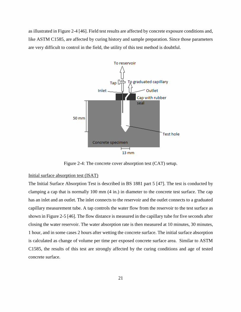
21

as illustrated in Figure 2-4 [46]. Field test results are affected by concrete exposure conditions and,

like ASTM C1585, are affected by curing history and sample preparation. Since those parameters

are very difficult to control in the field, the utility of this test method is doubtful.

Figure 2-4: The concrete cover absorption test (CAT) setup.

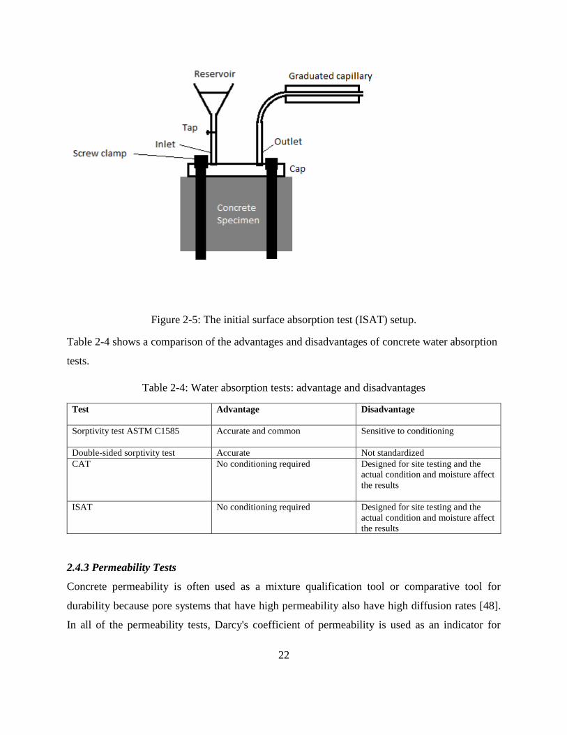
Initial surface absorption test (ISAT)

The Initial Surface Absorption Test is described in BS 1881 part 5 [47]. The test is conducted by

clamping a cap that is normally 100 mm (4 in.) in diameter to the concrete test surface. The cap

has an inlet and an outlet. The inlet connects to the reservoir and the outlet connects to a graduated

capillary measurement tube. A tap controls the water flow from the reservoir to the test surface as

shown in Figure 2-5 [46]. The flow distance is measured in the capillary tube for five seconds after

closing the water reservoir. The water absorption rate is then measured at 10 minutes, 30 minutes,

1 hour, and in some cases 2 hours after wetting the concrete surface. The initial surface absorption

is calculated as change of volume per time per exposed concrete surface area. Similar to ASTM

C1585, the results of this test are strongly affected by the curing conditions and age of tested

concrete surface.

22

Figure 2-5: The initial surface absorption test (ISAT) setup.

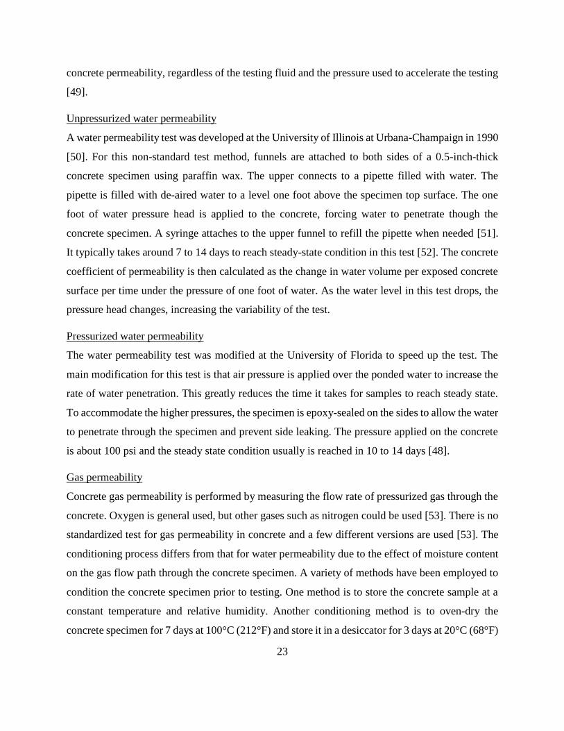
Table 2-4 shows a comparison of the advantages and disadvantages of concrete water absorption

tests.

Table 2-4: Water absorption tests: advantage and disadvantages

Test


Sorptivity test ASTM C1585 Accurate and common Sensitive to conditioning

Double-sided sorptivity test Accurate Not standardized

CAT No conditioning required Designed for site testing and the

actual condition and moisture affect

the results

ISAT No conditioning required Designed for site testing and the

actual condition and moisture affect

the results

2.4.3 Permeability Tests

Concrete permeability is often used as a mixture qualification tool or comparative tool for

durability because pore systems that have high permeability also have high diffusion rates [48].

In all of the permeability tests, Darcy's coefficient of permeability is used as an indicator for

23

concrete permeability, regardless of the testing fluid and the pressure used to accelerate the testing

[49].

Unpressurized water permeability

A water permeability test was developed at the University of Illinois at Urbana-Champaign in 1990

[50]. For this non-standard test method, funnels are attached to both sides of a 0.5-inch-thick

concrete specimen using paraffin wax. The upper connects to a pipette filled with water. The

pipette is filled with de-aired water to a level one foot above the specimen top surface. The one

foot of water pressure head is applied to the concrete, forcing water to penetrate though the

concrete specimen. A syringe attaches to the upper funnel to refill the pipette when needed [51].

It typically takes around 7 to 14 days to reach steady-state condition in this test [52]. The concrete

coefficient of permeability is then calculated as the change in water volume per exposed concrete

surface per time under the pressure of one foot of water. As the water level in this test drops, the

pressure head changes, increasing the variability of the test.

Pressurized water permeability

The water permeability test was modified at the University of Florida to speed up the test. The

main modification for this test is that air pressure is applied over the ponded water to increase the

rate of water penetration. This greatly reduces the time it takes for samples to reach steady state.

To accommodate the higher pressures, the specimen is epoxy-sealed on the sides to allow the water

to penetrate through the specimen and prevent side leaking. The pressure applied on the concrete

is about 100 psi and the steady state condition usually is reached in 10 to 14 days [48].

Gas permeability

Concrete gas permeability is performed by measuring the flow rate of pressurized gas through the

concrete. Oxygen is general used, but other gases such as nitrogen could be used [53]. There is no

standardized test for gas permeability in concrete and a few different versions are used [53]. The

conditioning process differs from that for water permeability due to the effect of moisture content

on the gas flow path through the concrete specimen. A variety of methods have been employed to

condition the concrete specimen prior to testing. One method is to store the concrete sample at a

constant temperature and relative humidity. Another conditioning method is to oven-dry the

concrete specimen for 7 days at 100°C (212°F) and store it in a desiccator for 3 days at 20°C (68°F)

24

[54]. A gas pressure is applied to one side of the concrete, and the gas flow rate through the

concrete is measured using a bubble flow meter (Kollek, 1989). The pressure used in one method

is about 5 bars and it takes about 40 minutes to several hours to reach a steady-state condition [49].

Other conditioning methods and gas pressures could be used; however, any differences would

change the measurements and limit comparisons.

Table 2-5 shows a comparison of the advantages and disadvantages of each concrete permeability

test method.

Table 2-5: Permeability tests: advantages and disadvantages

Test


Water permeability test Easy and simple. Long.

Pressurized water permeability

test

Higher pressure decreases test

time.

Setup is more complicated compared to

unpressurized water permeability test.

High pressure could damage sample.

Gas permeability test Faster test than water

permeability test.

Results dependent on conditioning

method.

2.4.4 Concrete Pore Volume and Size Distribution

The goal of a concrete porosity test is to find the interconnected void volume or the size profile of

the interconnected porosity of a concrete specimen. Concrete porosity is somewhat affected by the

porosity of aggregate since concrete consists mostly of aggregate; however, most of the voids in

concrete are in the paste [55]. While many different porosity tests have been developed for cement

paste and concrete, they each have limitations and none of them produce the same results. This

report will focus on two tests that have been developed for concrete. Mercury intrusion

porosimetry (MIP) and a boil test have been used extensively for cement paste and concrete [56].

Mercury intrusion porosimetry (MIP)

Mercury intrusion porosimetry is a commonly used test for determining the pore size profile for

cement-based materials including paste, mortar, and in some cases concrete. MIP is based on the

principle that a non-wetting liquid will intrude capillaries under high pressure, and that the

capillary size intruded is related to the pressure applied. Pore size distribution can be calculated

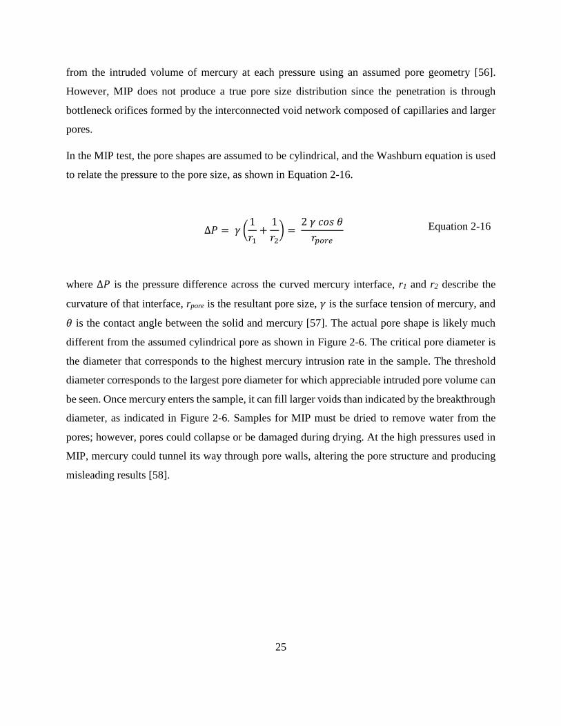
25

from the intruded volume of mercury at each pressure using an assumed pore geometry [56].

However, MIP does not produce a true pore size distribution since the penetration is through

bottleneck orifices formed by the interconnected void network composed of capillaries and larger

pores.

In the MIP test, the pore shapes are assumed to be cylindrical, and the Washburn equation is used

to relate the pressure to the pore size, as shown in Equation 2-16.

∆𝑃 = 𝛾 (

1

𝑟1+

1

𝑟2) =

2 𝛾 𝑐𝑜𝑠 𝜃

𝑟𝑝𝑜𝑟𝑒 Equation 2-16

where ∆𝑃 is the pressure difference across the curved mercury interface, r1 and r2 describe the

curvature of that interface, rpore is the resultant pore size, 𝛾 is the surface tension of mercury, and

𝜃 is the contact angle between the solid and mercury [57]. The actual pore shape is likely much

different from the assumed cylindrical pore as shown in Figure 2-6. The critical pore diameter is

the diameter that corresponds to the highest mercury intrusion rate in the sample. The threshold

diameter corresponds to the largest pore diameter for which appreciable intruded pore volume can

be seen. Once mercury enters the sample, it can fill larger voids than indicated by the breakthrough

diameter, as indicated in Figure 2-6. Samples for MIP must be dried to remove water from the

pores; however, pores could collapse or be damaged during drying. At the high pressures used in

MIP, mercury could tunnel its way through pore walls, altering the pore structure and producing

misleading results [58].

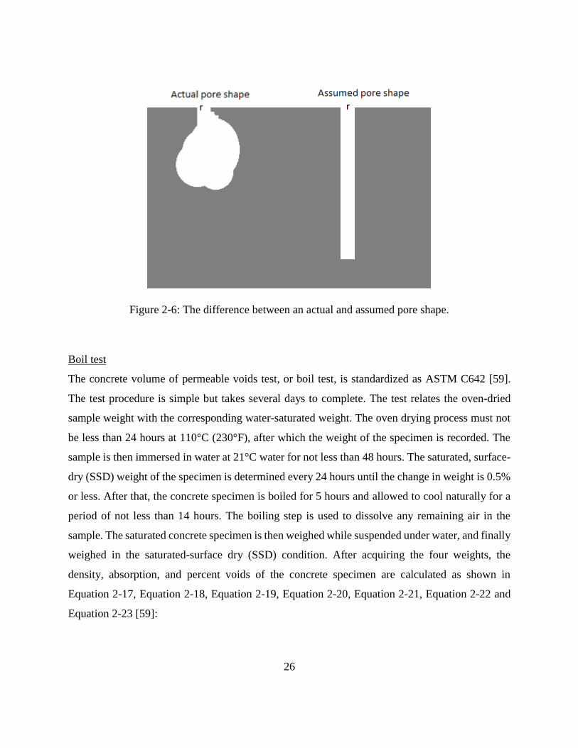
26

Figure 2-6: The difference between an actual and assumed pore shape.

Boil test

The concrete volume of permeable voids test, or boil test, is standardized as ASTM C642 [59].

The test procedure is simple but takes several days to complete. The test relates the oven-dried

sample weight with the corresponding water-saturated weight. The oven drying process must not

be less than 24 hours at 110°C (230°F), after which the weight of the specimen is recorded. The

sample is then immersed in water at 21°C water for not less than 48 hours. The saturated, surface-

dry (SSD) weight of the specimen is determined every 24 hours until the change in weight is 0.5%

or less. After that, the concrete specimen is boiled for 5 hours and allowed to cool naturally for a

period of not less than 14 hours. The boiling step is used to dissolve any remaining air in the

sample. The saturated concrete specimen is then weighed while suspended under water, and finally

weighed in the saturated-surface dry (SSD) condition. After acquiring the four weights, the

density, absorption, and percent voids of the concrete specimen are calculated as shown in

Equation 2-17, Equation 2-18, Equation 2-19, Equation 2-20, Equation 2-21, Equation 2-22 and

Equation 2-23 [59]:

27

𝐴𝑏𝑠𝑜𝑟𝑝𝑡𝑖𝑜𝑛 𝑎𝑓𝑡𝑒𝑟 𝑖𝑚𝑚𝑒𝑟𝑠𝑖𝑜𝑛 (%)= 𝐵−𝐴

𝐴×100 Equation 2-17

𝐴𝑏𝑠𝑜𝑟𝑝𝑡𝑖𝑜𝑛 𝑎𝑓𝑡𝑒𝑟 𝑖𝑚𝑚𝑒𝑟𝑠𝑖𝑜𝑛 𝑎𝑛𝑑 𝑏𝑜𝑖𝑙𝑖𝑛𝑔 (%)= 𝐶−𝐴

𝐴×100 Equation 2-18

𝐵𝑢𝑙𝑘 𝑑𝑒𝑛𝑠𝑖𝑡𝑦 (𝑑𝑟𝑦)= 𝐴

𝐶−𝐷∙𝜌=𝑔1 Equation 2-19

𝐵𝑢𝑙𝑘 𝑑𝑒𝑛𝑠𝑖𝑡𝑦 𝑎𝑓𝑡𝑒𝑟 𝑖𝑚𝑚𝑒𝑟𝑠𝑖𝑜𝑛= 𝐵

𝐶−𝐷∙𝜌 Equation 2-20

𝐵𝑢𝑙𝑘 𝑑𝑒𝑛𝑠𝑖𝑡𝑦 𝑎𝑓𝑡𝑒𝑟 𝑖𝑚𝑚𝑒𝑟𝑠𝑖𝑜𝑛 𝑎𝑛𝑑 𝑏𝑜𝑖𝑙𝑖𝑛𝑔= 𝐶

𝐶−𝐷∙𝜌 Equation 2-21

𝐴𝑝𝑝𝑎𝑟𝑒𝑛𝑡 𝑑𝑒𝑛𝑠𝑖𝑡𝑦= 𝐴

𝐴−𝐷∙𝜌=𝑔2 Equation 2-22

𝑉𝑜𝑙𝑢𝑚𝑒 𝑜𝑓 𝑝𝑒𝑟𝑚𝑒𝑎𝑏𝑙𝑒 𝑝𝑜𝑟𝑒 𝑠𝑝𝑎𝑐𝑒 (𝑣𝑜𝑖𝑑𝑠 %)= 𝑔2−𝑔1

𝑔2×100 𝑜𝑟

𝐶−𝐴

𝐶−𝐷×100

Equation 2-23

where A is the mass of the oven-dried sample in air (g), B is the mass of the saturated, surface-dry

sample in air after immersion (g), C is the mass of the saturated, surface-dry sample in air after

immersion and boiling (g), D is the apparent mass of the saturated sample suspended in water after

immersion and boiling (g), g1 = dry bulk density (Mg/m3), g2 = apparent density (Mg/m3), and ρ

= density of water (g/cm3).

Table 2-6 shows a comparison of the advantages and disadvantages of the concrete porosity tests.

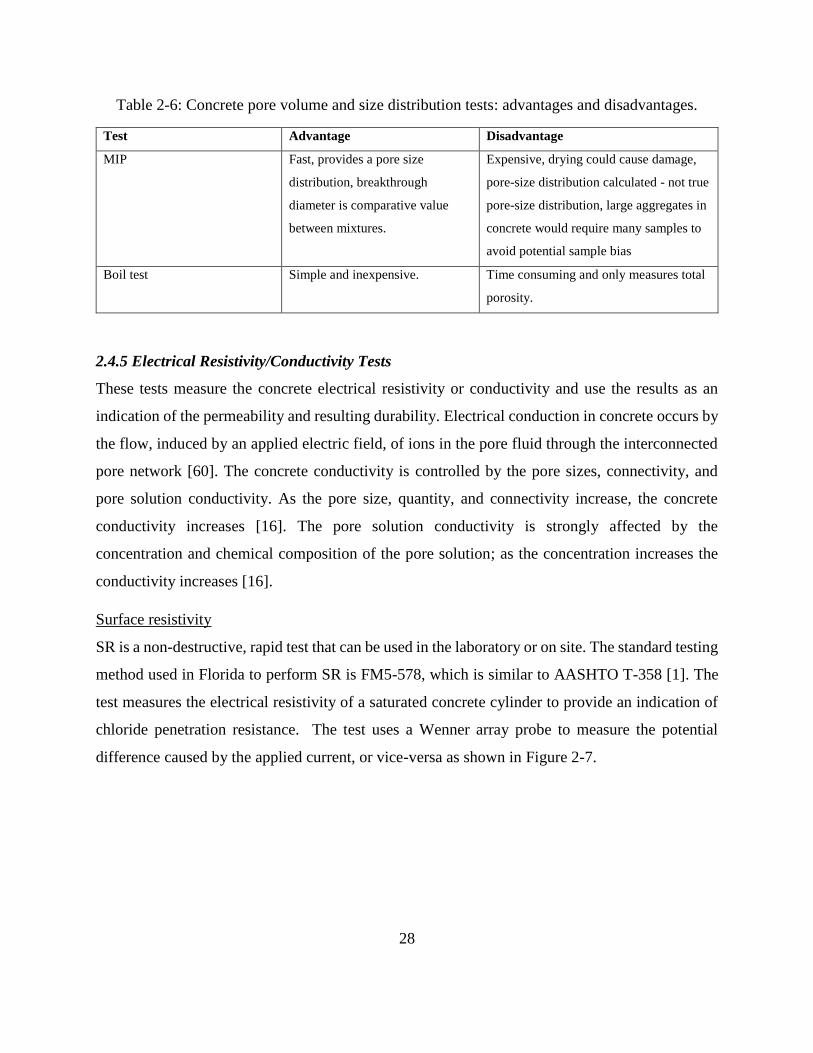
28

Table 2-6: Concrete pore volume and size distribution tests: advantages and disadvantages.

Test Advantage Disadvantage

MIP Fast, provides a pore size

distribution, breakthrough

diameter is comparative value

between mixtures.

Expensive, drying could cause damage,

pore-size distribution calculated - not true

pore-size distribution, large aggregates in

concrete would require many samples to

avoid potential sample bias

Boil test

Simple and inexpensive. Time consuming and only measures total

porosity.

2.4.5 Electrical Resistivity/Conductivity Tests

These tests measure the concrete electrical resistivity or conductivity and use the results as an

indication of the permeability and resulting durability. Electrical conduction in concrete occurs by

the flow, induced by an applied electric field, of ions in the pore fluid through the interconnected

pore network [60]. The concrete conductivity is controlled by the pore sizes, connectivity, and

pore solution conductivity. As the pore size, quantity, and connectivity increase, the concrete

conductivity increases [16]. The pore solution conductivity is strongly affected by the

concentration and chemical composition of the pore solution; as the concentration increases the

conductivity increases [16].

Surface resistivity

SR is a non-destructive, rapid test that can be used in the laboratory or on site. The standard testing

method used in Florida to perform SR is FM5-578, which is similar to AASHTO T-358 [1]. The

test measures the electrical resistivity of a saturated concrete cylinder to provide an indication of

chloride penetration resistance. The test uses a Wenner array probe to measure the potential

difference caused by the applied current, or vice-versa as shown in Figure 2-7.

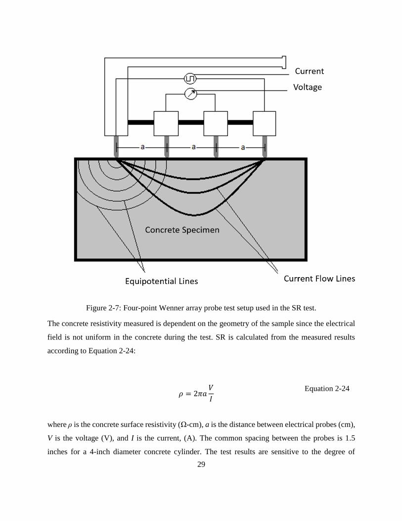
29

Figure 2-7: Four-point Wenner array probe test setup used in the SR test.

The concrete resistivity measured is dependent on the geometry of the sample since the electrical

field is not uniform in the concrete during the test. SR is calculated from the measured results

according to Equation 2-24:

𝜌 = 2𝜋𝑎

𝑉

𝐼

Equation 2-24

where ρ is the concrete surface resistivity (Ω-cm), a is the distance between electrical probes (cm),

V is the voltage (V), and I is the current, (A). The common spacing between the probes is 1.5

inches for a 4-inch diameter concrete cylinder. The test results are sensitive to the degree of

30

saturation and the saturation method, the pore solution conductivity, and temperature during

testing. Admixtures used in the concrete mixture that add ionic species to the pore solution, such

as calcium nitrite, increase the measured conductivity, which indicates that the concrete has a

higher permeability than its actual permeability [1]

Bulk resistivity

Bulk resistivity (BR) is similar to SR in concept but it measures the concrete resistivity through

the length of a concrete cylinder instead of just the surface, as shown in Figure 2-8. The BR test

method used in Florida is AASHTO TP119-15, which is the standard test for the uniaxial electrical

resistivity of a concrete cylinder [2]. BR can be measured using the same equipment as SR with

an attachment to connect Wenner surface resistivity meter probes to two conductive plates that go

on the ends of the cylinder. The end plates are typically electrically connected to the concrete

cylinder using saturated sponges. The electrical resistivity of the top and bottom saturated sponges

must be measured prior to testing so that the measured cylinder resistance can be corrected. BR is

often related to the chloride ion permeability classification using Table 2-7.

Figure 2-8: BR concrete specimen setup.

31

Table 2-7: Chloride ion permeability classification [2]

Chloride ion permeability classification BR (kΩ-cm)

High < 5.2

Moderate 5.2 - 10.4

Low 10.4 – 20.8

Very low 20.8 – 207

Negligible > 207

Rapid chloride permeability test (RCPT)

The Rapid chloride permeability test (RCPT) is a test that uses the total charge, driven by an

applied electric field of 60 Volts, passing through a 2-inch thick and 4-inch diameter concrete

sample over a period of 6 hours, as an index of the concrete permeability. This test has been

standardized as ASTM C1202 / AASHTO T 277 [3]. The specimens are vacuum-saturated with

de-aired water before testing [3]. An electrical current is conducted from the power source by

placing one end of the sample in a 0.3 N NaOH solution and the other end in a 3.0% NaCl solution.

Although the test is intended as an indirect measure of the concrete pore system network, anything

that changes the concrete resistivity will change the results. For example, certain admixtures such

as calcium nitrite change the pore solution conductivity and change the results. Likewise,

conductive fibers or aggregates that contain hematite can change the concrete electrical resistivity

without changing diffusion properties. Changes in the vacuum pressure used during saturation or

other specimen conditioning prior to testing can also change the sample resistivity due to the effect

of the degree of saturation of the tested specimen on the measured result. The change in

temperature due to high voltage passing through the specimen could affect the results as well [61].

Pore solution composition effect

Most of the electrical tests that are conducted on concrete to evaluate concrete resistivity or

conductivity are strongly affected by the concrete pore structure characteristics and pore solution

composition. The use of supplementary cementitious materials has an effect on the chemical

composition of the concrete pore solution due to the secondary reactions between CH and SCMs.

32

The consumption of hydroxyl ions in the pore solution causes an increase in the electrical

resistivity compared to the controlled ordinary concrete sample [62,63].

There are three known methods to find the pore solution composition in order to reflect its effect

on the concrete electrical conductivity. The first method involves pore solution extraction, which

was first used in 1970 and was performed by applying 370-MPa pressure on a cement paste

cylinder with a diameter of 45 mm and height of 80 mm. A bottom plate collects the expressed

pore solution and directs it through a Teflon tube into a syringe. Compositional testing on the

extracted pore solution must be performed immediately to avoid any changes in the chemical

characteristics of the pore solution. Each pore solution extraction process produces 4 – 10 ml of

pore solution, depending on the w/cm and the age of the specimen [64]. The second method

comprises using the Bentz pore solution electrical conductivity calculator, which is available

online http://concrete.nist.gov/poresolncalc.html. The calculator uses the chemical composition of

the cementitious materials and other factors to predict the pore solution electrical conductivity [7].

The third method uses a pore solution electrical conductivity sensor placed inside the concrete

specimen. The sensor is made of a porous material connected to electrodes in both ends, with a

known electrical conductivity in a saturated surface dry (SSD) condition. The porous material

absorbs the pore solution, which affects the electrical conductivity of the sensor. The difference in

conductivity between the SSD sensor and the sensor placed inside the concrete specimen is

considered the pore solution conductivity [16].

Formation factor

The correlation between the concrete and the pore solution conductivities is a result of the pore

sizes, distribution, and capillary connection of these pores as illustrated in Equation 2-25:

𝜌T

𝜌0=

1

𝛼𝛽= 𝐹 =

𝐷0

𝐷 Equation 2-25

where ρT is the concrete bulk resistivity (Ω-m), ρ0 is the pore solution resistivity (Ω-m), F is the

formation factor, D is the effective diffusion coefficient (m2/s), D0 is the ionic diffusion coefficient

in an infinitely dilute solution (m2/s), α is the pore volume fraction that contains fluid, and β is the

connectivity of the pores. The pore volume fraction coefficient (α) relates positively to the concrete

conductivity, as the porosity increases the electrical conductivity increases due to the increase in

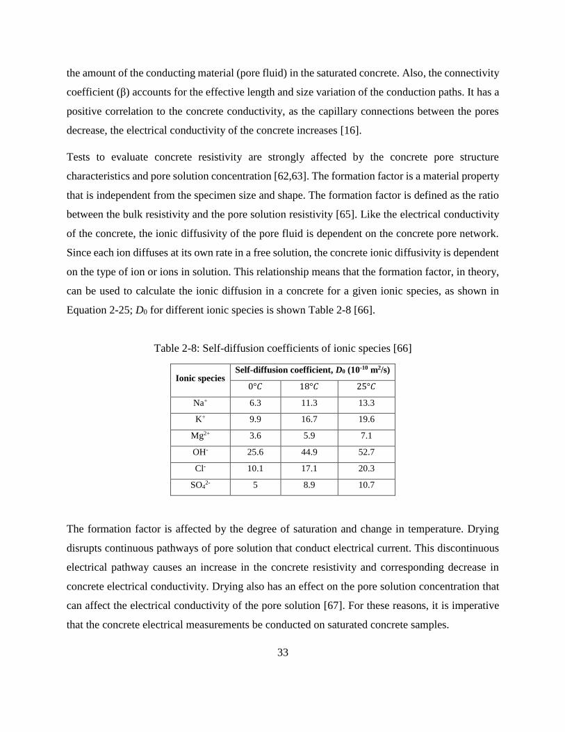
http://concrete.nist.gov/poresolncalc.html

33

the amount of the conducting material (pore fluid) in the saturated concrete. Also, the connectivity

coefficient (β) accounts for the effective length and size variation of the conduction paths. It has a

positive correlation to the concrete conductivity, as the capillary connections between the pores

decrease, the electrical conductivity of the concrete increases [16].

Tests to evaluate concrete resistivity are strongly affected by the concrete pore structure

characteristics and pore solution concentration [62,63]. The formation factor is a material property

that is independent from the specimen size and shape. The formation factor is defined as the ratio

between the bulk resistivity and the pore solution resistivity [65]. Like the electrical conductivity

of the concrete, the ionic diffusivity of the pore fluid is dependent on the concrete pore network.

Since each ion diffuses at its own rate in a free solution, the concrete ionic diffusivity is dependent

on the type of ion or ions in solution. This relationship means that the formation factor, in theory,

can be used to calculate the ionic diffusion in a concrete for a given ionic species, as shown in

Equation 2-25; D0 for different ionic species is shown Table 2-8 [66].

Table 2-8: Self-diffusion coefficients of ionic species [66]

Ionic species Self-diffusion coefficient, D0 (10-10 m2/s)

0°𝐶 18°𝐶 25°𝐶

Na+ 6.3 11.3 13.3

K+ 9.9 16.7 19.6

Mg2+ 3.6 5.9 7.1

OH- 25.6 44.9 52.7

Cl- 10.1 17.1 20.3

SO42- 5 8.9 10.7

The formation factor is affected by the degree of saturation and change in temperature. Drying

disrupts continuous pathways of pore solution that conduct electrical current. This discontinuous

electrical pathway causes an increase in the concrete resistivity and corresponding decrease in

concrete electrical conductivity. Drying also has an effect on the pore solution concentration that

can affect the electrical conductivity of the pore solution [67]. For these reasons, it is imperative

that the concrete electrical measurements be conducted on saturated concrete samples.

34

The effect of temperature changes is noticeable on the solubility of ions and the pore solution

composition. It also has an effect on the concrete microstructure at early ages [16]. The chemical

composition of the pore solution might be affected by the change in temperature. The increase in

temperature increases the solubility and concentration of ions in the pore solution and that

increases the concrete conductivity [68].

2.5 Supplementary Cementitious Materials

2.5.1 Background

Supplementary cementitious materials (SCM) can be divided into two main categories: pozzolanic

and hydraulic materials. Hydraulic cementitious materials react with water to produce a binder that

sets and hardens by chemical reaction with water and is stable under water. Hydraulic cements are

also capable of reacting under water. Examples of hydraulic materials include portland cement,

calcium aluminate cement, and slag cement. Pozzolanic materials are fine silicate or

aluminosilicate materials that react with calcium hydroxide at room temperature to produce

binding phases such as C-S-H or calcium aluminosilicate hydrate (C-A-S-H). Examples of

pozzolanic materials include silica fume, sugar can bagasse ash, and Class F fly ash. Some SCMs

such as slag and some Class C fly ashes can be both hydraulic and pozzolanic. SCMs are

frequently used in concrete to reduce concrete porosity and pore connectivity, mitigate alkali-silica

reaction and sulfate attack, or improve workability. The most commonly used SCMs in ternary

blends are fly ash, slag cement, and silica fume.

Fly ash

Fly ash is a by-product of coal-fired electric power plants. Fly ash particles travel with the flue gas

stream out of the boiler to filtration equipment such as electrostatic precipitators or bag filters

where they are captured. FA is categorized into two general classes, Class F fly ash and Class C

fly ash, as described in ASTM C618 [69]. Class F fly ash is produced by burning anthracite or

bituminous coal. For Class F fly ash, the sum of the silicon dioxide, aluminum oxide, and iron

oxide content must be at least 70 percent. This requirement means that Class F fly ash typically

has a low CaO content. Class C fly ash is produced by burning lignite or sub-bituminous coal. For

Class C fly ash, the sum of the silicon dioxide, aluminum oxide, and iron oxide content must be at

35

least 50 percent. This lower composition limit allows Class C fly ash to have high CaO contents

typically between 20 and 30 percent [12].

Class F fly ash is categorized as a pozzolanic material. Because of its high silica content, it reacts

with CH to form additional C-S-H and C-A-S-H to fill in voids and increase strength. It is used as

a partial replacement of portland cement [70]. Class F fly ash is often used to lower the heat of

hydration, improve workability, and mitigate alkali-silica reaction and sulfate attack. Class C fly

is both pozzolanic and hydraulic. Class C fly ash will sometimes contain C3A, gypsum/

hemihydrate, free lime, or other crystalline phases. For some Class C fly ash, the C3A and gypsum

can form monosulfoaluminate and ettringite to make the cementitious system perform poorly in

sulfate attack, and cause gypsum imbalance issues [19]. Free lime and the glassy material in the

fly ash will react in the high pH environment found in concrete to form C-S-H or C-A-S-H. Class

C fly ash is more reactive at early ages than Class F fly ash and is often preferred by contractors

because of the higher early strength gain rates [70].

Slag cement

Slag cement is a byproduct of the steel industry and predominantly consists of silicates and

aluminosilicates of lime and magnesia. The chemical and physical composition of slag cement are

strongly affected by the source and the plant’s main production material [71]. Slag is removed

from the molten ore during manufacture and rapidly chilled to lock in an amorphous structure and

increase reactivity. This rapid cooling produces small granules, mostly smaller than # 4 sieve that

are later ground into a fine powder. Partial portland cement replacement with slag cement typically

reduces early-age strength, but increases long term strength [72]. It also greatly reduces

permeability and can improve durability. It is often used to reduce the rate of heat development in

structural mass concrete and mitigate alkali-silica reaction. The effect of slag cement on hydration

is dominated by C/S and the alumina content. These reactions produce secondary C-S-H gel and

ettringite that fill in voids and reduce permeability [73].

Silica fume

Silica fume is a byproduct of the silicon and ferrosilicon industry. Silica fume color is typically

either white or gray, depending on the carbon content. Silica fume consists of extremely fine

particles between 0.1 and 0.2 µm in diameter. This makes silica fume particles 100 times smaller

36

than the average cement particle. It also gives silica fume an extremely high surface area between

13,000 and 30,000 m2/kg [12]. Silica fume requirements are given in ASTM C1240. To be used

in concrete, silica fume must be at least 85% SiO2, although it typically contains 92 to 97% SiO2.

Silica fume’s small particle size is known to increase strength and reduce permeability by

improving particle packing and acting as a nucleation site for C-S-H to form. The very high

amorphous silica content also makes it highly reactive in cementitious systems with small

replacement percentages. The use of silica fume as an SCM in concrete has been found to improve

compressive strength, bond strength, and durability [12].

Metakaolin

Metakaolin is a product of calcining clay containing typically high contents of kaolinite between

500 and 900°C. Metakaolin is considered a high quality mineral addition to concrete due to its

pozzolanic properties. The high alumina content of metakaolin makes it very effective in

mitigating alkali-silica reaction and delayed ettringite formation (DEF) in concrete. It is also very

effective in reducing concrete permeability through the formation of C-S-H, C-A-S-H and C-A-H

as a product of reacting with calcium hydroxide [12,60]. Metakaolin’s high surface area greatly

reduces the concrete workability; however, when used at relatively low levels of addition in ternary

blends, the loss of workability is minimized while still improving the durability.

2.5.2 Effect of Supplementary Cementitious Materials on Chloride Binding

Fly ash

The partial replacement of portland cement with fly ash increases the chloride binding capacity.

Chloride binding is significantly less effective in pastes containing fly ash exposed to external

chlorides than in those with premixed chlorides [32]. The increase in chloride binding can be

affected by the formation of secondary C-S-H, which causes the formation of physical bonding

between free chloride ions and the secondary C-S-H [24]. The high alumina content in fly ash

could affect chemical bond formation between free chloride ions and alumina to produce Friedel’s

salt [23,74]. The correlation between bound chloride and fly ash content seems to be linear up to

50% replacement of portland cement with fly ash [75]. The chloride binding of fly ash-cement

paste is strongly time-dependent and affected by the curing time and exposure period. In the case

37

of using fly ash as a supplementary cementitious material, as the curing age increases the chloride

binding capacity decreases for the same cementitious material composition [76]

Slag cement

Most studies show that increasing ground blast furnace slag content increases the chloride binding

capacity [23]. The free-chloride binding capacity of slag-cement paste with 66.7% slag cement is

about five times that of OPC paste. The use of slag cement in binary, ternary and quaternary blend

concrete mixtures increases magnesium content in the cementitious materials, which causes the

formation of hydrotalcite. Hydrotalcite has a positively charged outer layer that binds free chloride

ions in pore solution. Hydrotalcite binds chloride ions at a much higher rate than free hydroxyl

ions, causing a noticeable reduction in the Cl-/OH- ratio in the pore solution [77]. Slag cement also

participates in the formation of Friedel’s salt as a result of the alumina present in the slag; however,

hydrotalcite is responsible for a higher percentage of the chloride binding ability of slag concrete

[77].

Silica fume

Using silica fume as a partial replacement of portland cement reduces chloride binding capacity

regardless of the w/cm. This reduction occurs because silica fume reduces the C/S ratio of the C-

S-H. This reduction in the C/S ratio reduces the C-S-H binding capacity [23]. Silica fume also

decreases chloride binding by decreasing the pore solution pH and dilution of the C3A content of

the cementitious system, which causes a reduction in the Friedel’s salt formation [78]. The increase

in C–S–H from the silica fume pozzolanic reaction offsets some of the chloride binding reduction,

but not all [24].

Metakaolin

The use of metakaolin as a supplementary cementitious material will increase the chloride binding

capacity of a cementitious system regardless of the curing time [79]. Chloride binding with

metakaolin-cement paste is strongly dependent on the chloride concentration. In low

concentration, Friedel’s salt starts forming and then decomposes due to the formation of stratlingite

(C2ASH8). As the chloride content increases, the chloride binding increases, and the formation of

Friedel’s salt is stabilized. In high chloride concentrations, the absence of stratlingite is clear due

to the high stability of the formed Friedel’s salt [80].

38

2.5.3 Supplementary Cementitious Material Effect on Electrical Conductivity

The electrical conductivity of SCM mixes is lower than ordinary portland cement mixes due to

two major effects. SCMs reduce pore size volume, size, and connectivity through the formation of

pozzolanic products [68]. SCMs also change the pore solution composition and, consequently, the

pore solution conductivity.

Fly ash

Using fly ash as partial replacement of portland cement reduces the concentration of the pore

solution due to the pozzolanic reaction that decreases calcium hydroxide content and improves the

concrete microstructure. The reduction in pore connectivity and solution concentration causes a

conspicuous increase in the electrical resistivity [81].

Slag Cement

Slag cement increases the concrete electrical resistivity due to pozzolanic reactions that consume

calcium hydroxide, reduce pore connectivity, and reduce pore solution concentration. The effect

is controlled by the calcium oxide, alumina, and alkali contents [62,68].

Silica fume

Partial replacement of portland cement with silica fume causes a reduction in the induced electrical

charge, as well as in the measured corrosion current [77]. The reduction in C/S reduces the pH

value due to the consumption of calcium hydroxide in producing secondary C-S-H gel. This

process causes reduction in the pore solution concentration and conductivity, which affects the

electrical resistivity of concrete [23]. The pore size and connectivity are reduced due to the

formation of secondary C-S-H and consumption of soluble calcium hydroxide. This process

reduces the water permeability as well [23].

Metakaolin

The electrical resistivity of concrete increases when metakaolin is used as partial replacement of

portland cement. Some studies show that by using a 15% replacement, the electrical resistivity

increases 2 to 4 times [60]. The reduction is strongly affected by the reduction in permeability due

to the reaction between metakaolin and calcium hydroxide forming C-S-H, C-A-H, and C-A-S-H.

This reaction reduces the pore solution concentration due to the consumption of calcium

hydroxide, which will reduce the electrical conductivity of the pore solution [12,60].

39

CHAPTER 3. CONCRETE MIXTURE DESIGN

3.1 Type of Cement

Cement classification is dependent on the cement chemical composition and fineness [82]. The

cement C3A content affects the concrete chloride binding potential. The cement alkali content

strongly affects the pore solution composition and electrical conductivity. Cements with different

C3A contents and alkali contents were used in this project. Type IL cements with fine limestone

additions are increasingly being used in Florida and will also be included in this project. Since this

project is focused on cast-in-place concrete, this project focuses on cements used in Florida for

cast-in-place concrete. For this reason, type III cement was not studied in this project. Table 3-1

summarizes the concrete mixture proportions that the research team used in this study.

Table 3-1: Concrete mixture proportions

Mix

# Mix ID

Cement content (%) SCM Type (%)

w/cm Type

I/II

Type

V

Type

IL

Type I

HA

Fly

Ash

Slag

Cement

Silica

Fume Metakaolin

1 C-100 100 0.35

2 C-100h 100 0.44

3 C-F10 90 10 0.35

4 C-F20 80 20 0.35

5 C-F10h 90 10 0.44

6 C-F20h 80 20 0.44

7 C-G60 40 60 0.35

8 C-S8 92 8 0.35

9 C-M10 90 10 0.35

10 C-F10G30 60 10 30 0.35

11 C-F10G45 45 10 45 0.35

12 C-F10G60 30 10 60 0.35

13 C-F10G60h 30 10 60 0.44

14 C-F20S4 76 20 4 0.35

15 C-F20S6 74 20 6 0.35

16 C-F20S8 72 20 8 0.35

17 C-F20S8h 72 20 8 0.44

18 C-F20M6 74 20 6 0.35

19 C-F20M8 72 20 8 0.35

20 C-F20M10 70 20 10 0.35

40

Mix

# Mix ID

Cement content (%) SCM Type (%)

w/cm Type

I/II

Type

V

Type

IL

Type I

HA

Fly

Ash

Slag

Cement

Silica

Fume Metakaolin

21 C-F20M10h 70 20 10 0.44

22 C-G55M8 37 55 8 0.35

23 C-G55M10 35 55 10 0.35

24 CV-100 100 0.35

25 CV-100h 100 0.44

26 CV-F10G60 30 10 60 0.35

27 CV-F20S8 72 20 8 0.35

28 CV-M10 90 10 0.35

29 CL-100 100 0.35

30 CL-100h 100 0.44

31 CL-F10G60 30 10 60 0.35

32 CL-F20S8 72 20 8 0.35

33 CL-M10 90 10 0.35

34 CHA-100 100 0.35

35 CHA-100h 100 0.44

36 CHA-

F10G60 30 10 60 0.35

37 CHA-F20S8 72 20 8 0.35

38 CHA-M10 90 10 0.35

3.1.1 Type I/II

ASTM C150 [83] Type I/II cement is the most commonly used cement in the Florida concrete

industry. The type I/II cement was the control cement for this study. Variation in the other cement

types was used to address the effect of the chemical composition on transport properties, chloride

binding, and sulfate attack durability.

3.1.2 Type V

The main difference between ASTM C150 type I/II and ASTM C150 type V cements is the C3A

content. Type V cement must have a C3A content lower than 5% in order to improve the concrete

sulfate attack resistance. Type V cement is not available in Florida and the FDOT standard suggests

using type I/II cement with slag or pozzolan instead of type V cement in aggressive environments

41

[84]. A cement with a C3A content of 2.2% was used in this study to address the effect of reducing

the C3A content on chloride binding and sulfate attack durability.

3.1.3 Type IL

Type IL cement is a type I or I/II cement with limestone additions up to 15% of the total cement

by weight. Limestone additions help improve the cement’s strength, durability, and plastic

properties [82]. This type of cement is not commonly used yet by FDOT-sponsored construction

projects; however, it is expected that in the near future it will be commonly used [84].

3.1.4 High Alkali Cement (HA)

Cement alkali content is typically reported as the sodium-equivalent alkali content, Na2Oeq. It is

calculated using the sodium and potassium content in the cement as shown in Equation 3-1[84]:

Na2Oeq = Na2O + (0.658 × K2O) Equation 3-1

where Na2O is the sodium oxide content in the cement by mass (%), and K2O is the potassium

oxide content in the cement by mass. In Equation 3-1, K2O is multiplied by 0.658 to account for

the difference in molecular weight between K2O and Na2O. Most cements used in Florida have a

Na2Oeq content below 0.6%. A cement with an alkali content between 0.8 and 1.0 was procured

for use in this project. Differences in the cement alkali content are responsible for most differences

in the pore solution electrical conductivity based on cement type. Inclusion of a high-alkali cement

may determine if the formation factor can account for differences seen in electrical tests conducted.

3.2 Supplementary Cementitious Materials

Supplementary cementitious materials (SCMs) are used in concrete to improve the concrete

strength, workability, and durability [85]. SCMs greatly reduce concrete transport properties and

change the pore solution electrical conductivity. In this project, concrete mixtures without SCMs,

with binary blends, and with ternary concrete blends were made to study the synergistic effect of

using multiple SCMs, as shown in Table 3-1. Four commonly used SCMs were used in this project

[8]. Binary concrete blends are mixtures that have one supplementary cementitious material (SCM)

to improve concrete properties, while ternary blends contain two SCMs in addition to the cement.

42

In this project, limestone fines were not treated as SCM additions, but as part of the cement. For

example, in this study, a type IL cement with fly ash would be considered a binary blend, not a

ternary blend. In this project, ten binary concrete mixtures were made to assess the effect of each

SCM independently on the concrete electrical, transport, and durability properties. SCMs have

positive effects and negative effects on different properties. For example, fly ash could reduce the

concrete early strength but increase the ultimate strength [86]. Multiple SCMs are sometimes used

in concrete mixtures to positively impact more concrete properties than possible by an individual

SCM. For example, silica fume will increase the early-age concrete strength, while fly ash will

increase the later-age concrete strength. In this project, sixteen ternary concrete mixtures were used

to address the effect of multiple SCMs on the concrete electrical, transport, and durability

properties.

3.2.1 Fly Ash

In this project, twenty-two concrete mixtures were made with an ASTM C618 [69] Class F fly ash.

The Class F fly ash was used at a 10 or 20% equivalent weight replacement of portland cement, as

shown in Table 3-1, to study the influence of fly ash content on concrete properties. These dosages

were selected because they are commonly used in FDOT ternary mixtures.

3.2.2 Slag Cement

In this project, an ASTM C989 [87] grade 120 slag cement was procured for use in this study. As

shown in Table 3-1, ten concrete mixtures will use slag cement at 30, 45, 55, or 60% equivalent

weight replacement of portland cement to address the effect of slag in binary and ternary blends

concrete. These dosages were selected to study the effect of slag cement dosage on water transport

properties and because these dosages have been used in FDOT concrete mixtures.

3.2.3 Silica Fume

An ASTM C1240 [88]-compliant silica fume was procured for use in this project. In this project,

nine concrete mixtures used silica fume as an SCM at 4, 6, or 8% equivalent weight replacement

of portland cement. As illustrated in Table 3-1, 8% addition was selected to comply with the 7-9%

silica fume usage range in approved FDOT concrete mixtures [8]. Lower dosages were also used

in this study to see the effects of dosage on the concrete transport properties and electrical

conductivity.

43

3.2.4 Metakaolin

A commercially-available metakaolin was procured for use in this project. The use of metakaolin

as an SCM in this project was limited to nine concrete mixtures using 6, 8, or 10% equivalent

weight replacement of portland cement, as shown in Table 3-1. Metakaolin was selected for fewer

mixtures in this study because it is used in FDOT ternary mixtures less frequently than the other

SCMs [8].

3.3 Aggregates

Aggregates were selected that are representative of FDOT mixtures and are compatible with the

test requirements.

3.3.1 Coarse Aggregates

An ASTM C33 [89] #57 Brooksville limestone was used in all of the concrete mixtures shown in

Table 3-1. Concrete Mixtures 1 and 16 were reproduced using an ASTM C33 #89 Miami Oolite

limestone to determine the effects of aggregate size on MIP sample results and labeled as mixtures

39 and 40.

3.3.2 Fine Aggregates

A locally available, ASTM C33 natural siliceous concrete sand was procured for use in this project.

A fixed coarse-aggregate–to-fine-aggregate ratio was used for all mixtures with the total quantities

of each adjusted based on the volume of paste used in each mixture.

3.4 Chemical Admixtures

Chemical admixtures are added to FDOT concrete mixtures to improve workability, decrease

water-to-cementitious material ratio (w/cm), increase strength, reduce concrete transport

properties, and increase durability in extremely aggressive environments [85]. An ASTM C494

[90] Type F high-range water-reducing admixture was used in the concrete mixtures. The high-

range water-reducing admixture dosage was altered for each mixture for workability.

In this project, two w/cm ratios, 0.35 and 0.44 were used to determine the effect of w/cm. The 0.35

ratio was chosen because it is the w/cm required when silica fume is used (0.35), and 0.44 was

44

chosen because it is the maximum approved by FDOT for use in Class IV concrete mix designs

(the class used in this study) [84].

45

CHAPTER 4. MATERIALS CHARACTERIZATION

4.1 Aggregate Properties

The coarse aggregate used in this project was a Miami Oolite limestone. The coarse aggregate

specific gravity and absorption were measured according to ASTM C127 [91] and are shown in

Table 4-1. The coarse aggregate particle size distribution was measured according to ASTM C136

[92] and is shown in Table 4-2.

Table 4-1: Coarse aggregate specific gravity and absorption

Property Value

Bulk specific gravity dry 2.29

Bulk specific gravity SSD 2.40

Apparent specific gravity 2.56

Absorption (%) 4.66

Table 4-2: Coarse aggregate particle size distribution

Sieve Size Percent Passing FDOT Specification

1 ½” 100 100

1” 99.8 95-100

¾” 92.7 ---

½” 45.6 25-60

3/8” 19.1 ---

No. 4 5.3 0-10

No. 8 4.7 0-5

The fine aggregate used in this project was a Georgia silica sand. The fine aggregate specific

gravity and absorption were measured according to ASTM C128 [93] and are shown in Table 4-

3, and the sieve analysis gradation was performed according to ASTM C 136 and is shown in

Table 4-4.

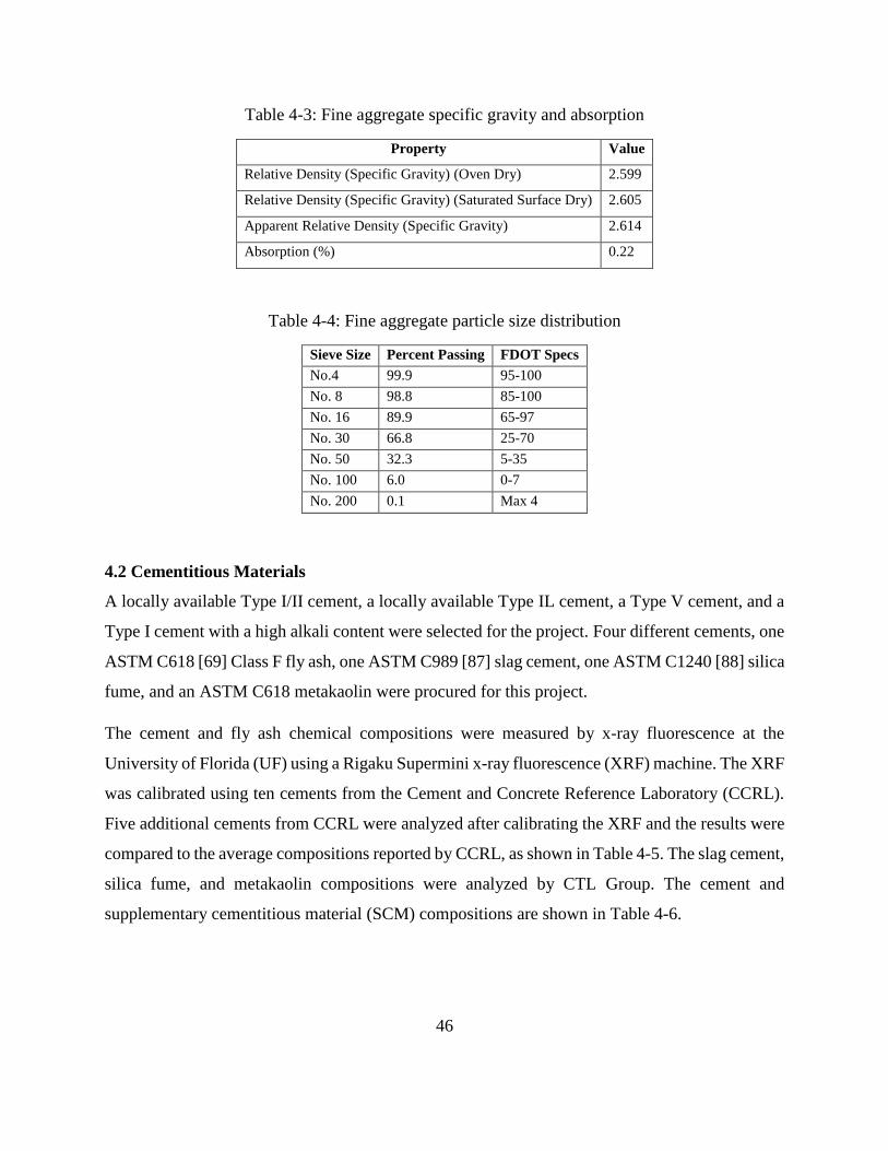
46

Table 4-3: Fine aggregate specific gravity and absorption

Property Value

Relative Density (Specific Gravity) (Oven Dry) 2.599

Relative Density (Specific Gravity) (Saturated Surface Dry) 2.605

Apparent Relative Density (Specific Gravity) 2.614

Absorption (%) 0.22

Table 4-4: Fine aggregate particle size distribution

Sieve Size Percent Passing FDOT Specs

No.4 99.9 95-100

No. 8 98.8 85-100

No. 16 89.9 65-97

No. 30 66.8 25-70

No. 50 32.3 5-35

No. 100 6.0 0-7

No. 200 0.1 Max 4

4.2 Cementitious Materials

A locally available Type I/II cement, a locally available Type IL cement, a Type V cement, and a

Type I cement with a high alkali content were selected for the project. Four different cements, one

ASTM C618 [69] Class F fly ash, one ASTM C989 [87] slag cement, one ASTM C1240 [88] silica

fume, and an ASTM C618 metakaolin were procured for this project.

The cement and fly ash chemical compositions were measured by x-ray fluorescence at the

University of Florida (UF) using a Rigaku Supermini x-ray fluorescence (XRF) machine. The XRF

was calibrated using ten cements from the Cement and Concrete Reference Laboratory (CCRL).

Five additional cements from CCRL were analyzed after calibrating the XRF and the results were

compared to the average compositions reported by CCRL, as shown in Table 4-5. The slag cement,

silica fume, and metakaolin compositions were analyzed by CTL Group. The cement and

supplementary cementitious material (SCM) compositions are shown in Table 4-6.

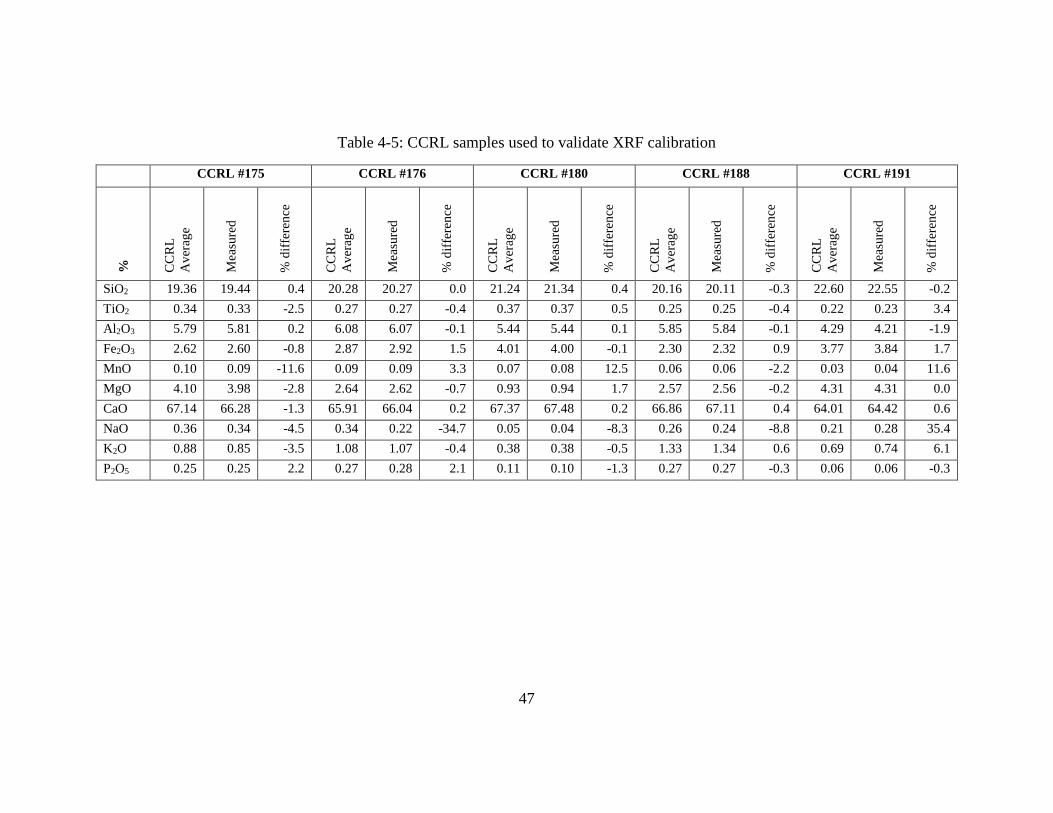
47

Table 4-5: CCRL samples used to validate XRF calibration

CCRL #175 CCRL #176 CCRL #180 CCRL #188 CCRL #191

%

CC

RL

Av

erag

e

Mea

sure

d

% d

iffe

ren

ce

CC

RL

Av

erag

e

Mea

sure

d

% d

iffe

ren

ce

CC

RL

Av

erag

e

Mea

sure

d

% d

iffe

ren

ce

CC

RL

Av

erag

e

Mea

sure

d

% d

iffe

ren

ce

CC

RL

Av

erag

e

Mea

sure

d

% d

iffe

ren

ce

SiO2 19.36 19.44 0.4 20.28 20.27 0.0 21.24 21.34 0.4 20.16 20.11 -0.3 22.60 22.55 -0.2

TiO2 0.34 0.33 -2.5 0.27 0.27 -0.4 0.37 0.37 0.5 0.25 0.25 -0.4 0.22 0.23 3.4

Al2O3 5.79 5.81 0.2 6.08 6.07 -0.1 5.44 5.44 0.1 5.85 5.84 -0.1 4.29 4.21 -1.9

Fe2O3 2.62 2.60 -0.8 2.87 2.92 1.5 4.01 4.00 -0.1 2.30 2.32 0.9 3.77 3.84 1.7

MnO 0.10 0.09 -11.6 0.09 0.09 3.3 0.07 0.08 12.5 0.06 0.06 -2.2 0.03 0.04 11.6

MgO 4.10 3.98 -2.8 2.64 2.62 -0.7 0.93 0.94 1.7 2.57 2.56 -0.2 4.31 4.31 0.0

CaO 67.14 66.28 -1.3 65.91 66.04 0.2 67.37 67.48 0.2 66.86 67.11 0.4 64.01 64.42 0.6

NaO 0.36 0.34 -4.5 0.34 0.22 -34.7 0.05 0.04 -8.3 0.26 0.24 -8.8 0.21 0.28 35.4

K2O 0.88 0.85 -3.5 1.08 1.07 -0.4 0.38 0.38 -0.5 1.33 1.34 0.6 0.69 0.74 6.1

P2O5 0.25 0.25 2.2 0.27 0.28 2.1 0.11 0.10 -1.3 0.27 0.27 -0.3 0.06 0.06 -0.3

48

Table 4-6: Cement and supplementary cementitious material composition as measured by XRF

Material SiO2 TiO2 Al2O3 Fe2O3 MnO MgO CaO Na2O K2O P2O5 LOI

wt% wt% wt% wt% wt% wt% wt% wt% wt% wt% wt%

Cement IL(11) 19.93 0.39 4.47 3.63 0.02 0.86 64.03 0.07 0.33 0.10 5.21

Cement type V 20.83 0.21 4.12 3.88 0.16 0.87 66.24 0.02 0.62 0.11 2.86

Cement type I/II 21.00 0.23 5.06 3.28 0.08 0.68 66.74 0.10 0.24 0.15 3.02

High alkali cement 20.56 0.21 4.55 3.78 0.09 3.06 63.65 0.29 0.87 0.12 2.68

Class F Fly Ash 48.59 1.00 19.49 19.68 0.04 0.84 5.08 0.83 2.09 0.12 1.88

Slag 34.1 0.58 14.04 0.59 0.25 5.45 41.27 0.23 0.24 0.01 0.47

Silica fume 87.67 <0.01 0.34 0.89 0.09 6.71 0.63 0.75 0.99 0.10 3.12

Metakaolin 52.53 1.8 42.96 1.49 <0.01 0.18 <0.01 0.05 0.14 0.15 1.46

49

The cement crystalline compositions were analyzed using x-ray diffraction and Rietveld

refinement. The x-ray diffraction patterns were collected using a 0.008 2θ step size, 10 seconds

per step, and Cu K. radiation. The open-source software Profex 3.11.1 was used to perform the

Rietveld refinement. The resolved cement compositions are shown in Table 4-7.

Table 4-7: Cement composition analyzed by X-Ray diffraction and Rietveld refinement

Phase Type I/II Type V IL(11) High Alkali Type I/II

Alite (%) 49.87 59.80 49.98 53.29

Belite (%) 18.34 11.52 14.78 19.27

Aluminate (%) 9.73 2.21 4.41 3.79

Ferrite (%) 10.33 15.36 13.93 14.52

Anhydrite (%) 0.55 0.41 0.37 0.56

Bassanite (%) 0.00 2.53 3.11 0.64

Gypsum (%) 5.22 1.25 0.77 3.47

Arcanite (%) 0.87 0.40 0.51 1.39

Calcite (%) 3.97 5.78 10.73 0.98

Free Lime (%) 0.79 0.00 0.39 0.19

MgO (%) 0.32 0.74 0.05 1.90

Quartz (%) 0.00 0.00 0.96 0.00

50

CHAPTER 5. SPECIMEN FABRICATION FOR TRANSPORT AND ELECTRICAL

PROPERTY TESTING

5.1 Concrete Methodology

Cylinders used for measuring concrete transport and electrical properties were made according to

ASTM C192, Standard Practice for Making and Curing Concrete Test Specimens in the

Laboratory [94]. All concrete batches were made in the concrete mixing facilities at the University

of Florida (UF).

5.1.1 Concrete Mixing

Three days prior to mixing, the coarse aggregate was soaked in a water tub, and the fine aggregate

was oven-dried at 230°F (110°C). One day prior to mixing, all the aggregates and cementitious

materials were weighed and sealed using five-gallon buckets. On the day of mixing, the mixer was

rinsed with water to clean it and buttered with fine aggregates, cement, and water to compensate

for mortar loss when fresh concrete is discharged from the mixer. After that, the coarse and fine

aggregate were added to the mixer and mixed for 30 seconds. While the mixer was running, the

cementitious materials and more than half of the mixing water were added. The admixtures and

the remaining water were added gradually over about one minute. The total mixing time for adding

all the materials was about three minutes, followed by a three-minute rest, and followed by mixing

for two additional minutes. After the mixing was done, the fresh concrete properties were

measured.

5.1.2 Fresh Concrete Properties

Standard concrete fresh quality control tests were performed [95-98]. Concrete slump was

measured according to ASTM C143 “Standard Test Method for Slump of Hydraulic-Cement

Concrete” [95] as shown in Figure 5-1. For most of the batches made, the slump values were

between 1.5 and 7.5 in. (38 and 191 mm).

51

Figure 5-1: Determination of slump

The unit weight test is used to verify the density of fresh concrete for quality control purposes and

can help pick up problems with incorrect ingredients or air content. This test was performed

according to ASTM C138 “Standard Test Method for Density (Unit Weight), Yield, and Air

Content (Gravimetric) of Concrete” [96] as shown in Figure 5-2. For most of the mixtures made,

the unit weight values were 139 to 144 lb/ft3 (2227 to 2307 kg/m3).

Figure 5-2: Determination of unit weight

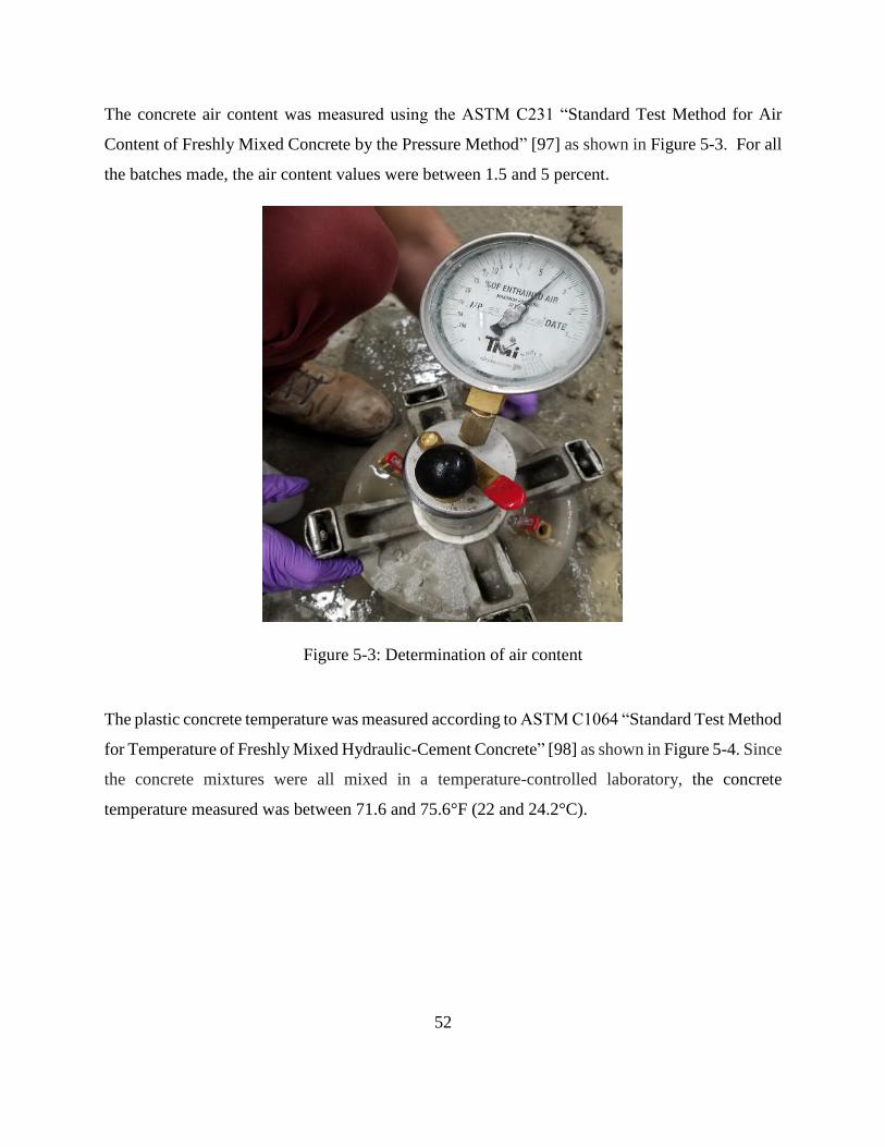
52

The concrete air content was measured using the ASTM C231 “Standard Test Method for Air

Content of Freshly Mixed Concrete by the Pressure Method” [97] as shown in Figure 5-3. For all

the batches made, the air content values were between 1.5 and 5 percent.

Figure 5-3: Determination of air content

The plastic concrete temperature was measured according to ASTM C1064 “Standard Test Method

for Temperature of Freshly Mixed Hydraulic-Cement Concrete” [98] as shown in Figure 5-4. Since

the concrete mixtures were all mixed in a temperature-controlled laboratory, the concrete

temperature measured was between 71.6 and 75.6°F (22 and 24.2°C).

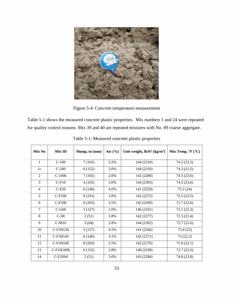
53

Figure 5-4: Concrete temperature measurement

Table 5-1 shows the measured concrete plastic properties. Mix numbers 1 and 24 were repeated

for quality control reasons. Mix 39 and 40 are repeated mixtures with No. 89 coarse aggregate.

Table 5-1: Measured concrete plastic properties

Mix No Mix ID Slump, in (mm) Air (%) Unit weight, lb/ft3 (kg/m3) Mix Temp, °F (°C)

1 C-100 7 (165) 3.2% 144 (2310) 74.3 (23.5)

1r C-100 6 (152) 3.0% 144 (2310) 74.3 (23.5)

2 C-100h 7 (165) 2.0% 142 (2280) 74.5 (23.6)

3 C-F10 4 (102) 3.0% 144 (2303) 74.5 (23.6)

4 C-F20 6 (140) 4.0% 141 (2259) 75.2 (24)

5 C-F10h 8 (191) 3.0% 142 (2272) 72.5 (22.5)

6 C-F20h 8 (203) 3.5% 142 (2269) 72.7 (22.6)

7 C-G60 5 (127) 2.0% 146 (2331) 72.1 (22.3)

8 C-S8 2 (51) 3.8% 142 (2277) 72.3 (22.4)

9 C-M10 3 (64) 2.8% 144 (2302) 72.7 (22.6)

10 C-F10G30 5 (127) 4.5% 141 (2266) 73.4 (23)

11 C-F10G45 6 (140) 3.1% 142 (2271) 72 (22.2)

12 C-F10G60 8 (203) 2.5% 142 (2276) 71.8 (22.1)

13 C-F10G60h 6 (152) 2.8% 140 (2249) 72.7 (22.6)

14 C-F20S4 2 (51) 3.0% 143 (2284) 74.8 (23.8)

54

Mix No Mix ID Slump, in (mm) Air (%) Unit weight, lb/ft3 (kg/m3) Mix Temp, °F (°C)

15 C-F20S6 3 (64) 3.4% 142 (2282) 75.4 (24.1)

16 C-F20S8 6 (152) 5.0% 141 (2262) 74.1 (23.4)

17 C-F20S8h 6 (152) 1.6% 140 (2244) 72.1 (22.3)

18 C-F20M6 4 (102) 3.4% 141 (2252) 73.8 (23.2)

19 C-F20M8 2 (51) 4.0% 144 (2305) 73.8 (23.2)

20 C-F20M10 2 (51) 2.5% 145 (2316) 73.6 (23.1)

21 C-F20M10h 6 (152) 2.0% 141 (2261) 73.9 (23.3)

22 C-G55S8 3 (64) 3.5% 140 (2240) 72.5 (22.5)

23 C-G55M10 2 (51) 2.5% 140 (2240) 72.7 (22.6)

24 CV-100 9 (229) 7.5% 131 (2098) 74.3 (23.5)

24r CV-100 3 (64) 2.75% 144 (2309) 74.7 (23.7)

25 CV-100h 6 (152) 1.5% 140 (2249) 75.4 (24.1)

26 CV-F10G60 7 (178) 3.0% 142 (2278) 71.8 (22.1)

27 CV-F20S8 4 (89) 4.5% 140 (2240) 73 (22.8)

28 CV-M10 3 (70) 3.1% 142 (2267) 72.7 (22.6)

29 CL-100 4 (108) 3.5% 141 (2258) 76.5 (24.7)

30 CL-100h 5 (114) 4.0% 140 (2239) 76.8 (24.9)

31 CL-F10G60 5 (127) 3.2% 142 (2277) 71.6 (22)

32 CL-F20S8 3 (64) 4.0% 139 (2228) 75.6 (24.2)

33 CL-M10 2 (38) 2.7% 144 (2307) 75.2 (24)

34 CHA-100 3 (83) 3.0% 143 (2284) 75 (23.9)

35 CHA-100h 7 (184) 2.8% 142 (2269) 75.6 (24.2)

36 CHA-F10G60 5 (114) 3.2% 141 (2255) 71.8 (22.1)

37 CHA-F20S8 3 (64) 4.0% 140 (2239) 74.8 (23.8)

38 CHA-M10 2 (51) 2.5% 140 (2239) 74.7 (23.7)

39 C-100 1 (25) 2.5% 145 (2323) 74.7 (23.7)

40 C-F20S8 1 (25) 2 141 (2264) 75.2 (24)

5.1.3 Concrete Specimen Preparation

After measuring the fresh concrete properties, 4 × 8 in. (100 × 200 mm) concrete cylinders and 4

× 4 × 11.25 in. (100 × 100 × 286 mm) concrete prisms were made according to ASTM C192 [94].

The concrete was placed into the cylinder molds and prism molds in two equal layers as shown in

Figure 5-5 and Figure 5-6. The concrete samples were consolidated using vibration from a

55

vibrating table. After the concrete was placed in the cylinder molds, they were finished and capped

to prevent moisture loss during the first 24 hours. The prisms were covered in plastic for the first

24 hours after mixing.

Figure 5-5: Cylinders after being filled with the first layer of concrete

Figure 5-6: Concrete prism mold after first layer of concrete added

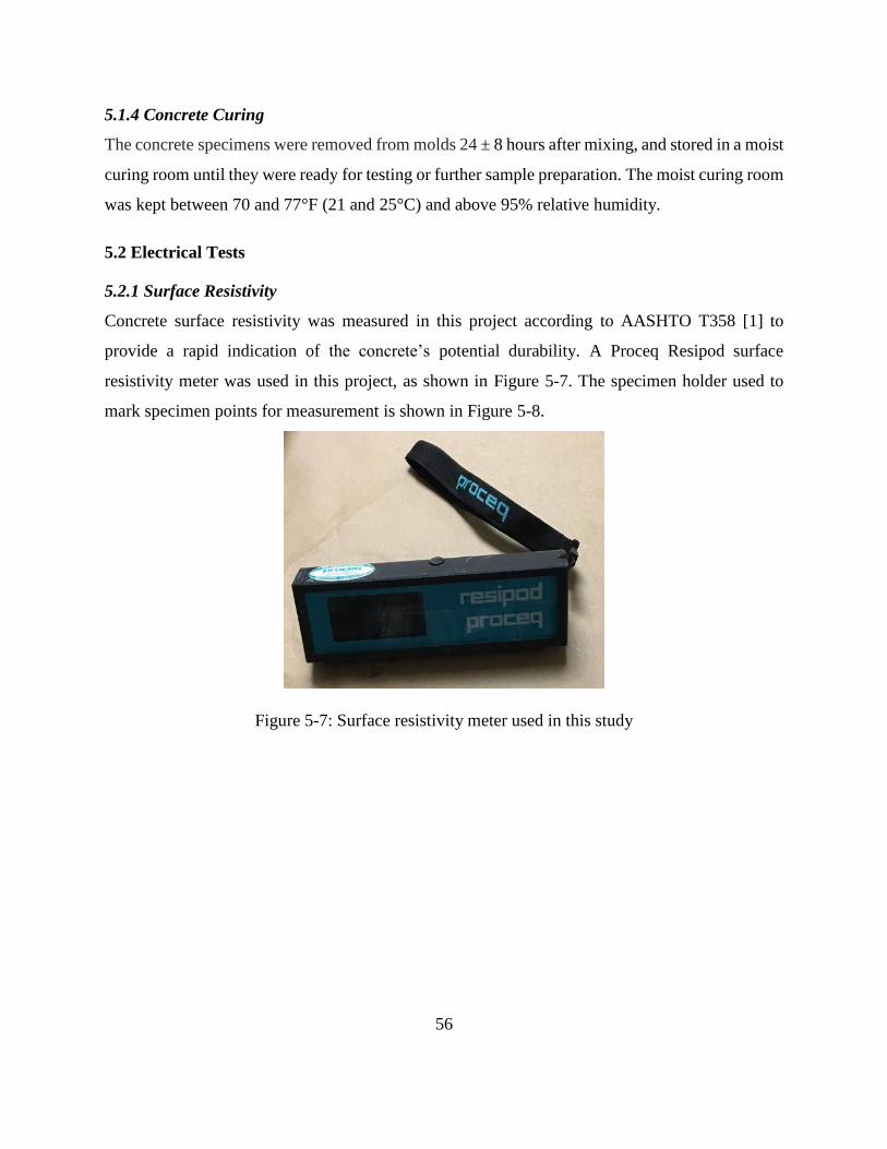
56

5.1.4 Concrete Curing

The concrete specimens were removed from molds 24 ± 8 hours after mixing, and stored in a moist

curing room until they were ready for testing or further sample preparation. The moist curing room

was kept between 70 and 77°F (21 and 25°C) and above 95% relative humidity.

5.2 Electrical Tests

5.2.1 Surface Resistivity

Concrete surface resistivity was measured in this project according to AASHTO T358 [1] to

provide a rapid indication of the concrete’s potential durability. A Proceq Resipod surface

resistivity meter was used in this project, as shown in Figure 5-7. The specimen holder used to

mark specimen points for measurement is shown in Figure 5-8.

Figure 5-7: Surface resistivity meter used in this study

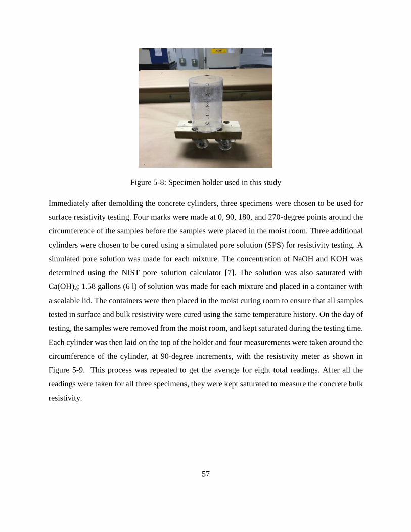
57

Figure 5-8: Specimen holder used in this study

Immediately after demolding the concrete cylinders, three specimens were chosen to be used for

surface resistivity testing. Four marks were made at 0, 90, 180, and 270-degree points around the

circumference of the samples before the samples were placed in the moist room. Three additional

cylinders were chosen to be cured using a simulated pore solution (SPS) for resistivity testing. A

simulated pore solution was made for each mixture. The concentration of NaOH and KOH was

determined using the NIST pore solution calculator [7]. The solution was also saturated with

Ca(OH)2; 1.58 gallons (6 l) of solution was made for each mixture and placed in a container with

a sealable lid. The containers were then placed in the moist curing room to ensure that all samples

tested in surface and bulk resistivity were cured using the same temperature history. On the day of

testing, the samples were removed from the moist room, and kept saturated during the testing time.

Each cylinder was then laid on the top of the holder and four measurements were taken around the

circumference of the cylinder, at 90-degree increments, with the resistivity meter as shown in

Figure 5-9. This process was repeated to get the average for eight total readings. After all the

readings were taken for all three specimens, they were kept saturated to measure the concrete bulk

resistivity.

58

Figure 5-9: Surface resistivity measurement

5.2.2 Bulk Resistivity

This concrete bulk resistivity was measured according to AASHTO TP 119 [2] to provide a rapid

indication of concrete mixture durability. The electrical current passes along the height (bulk) of

the cylinder in the bulk resistivity test, while with the surface resistivity test, the electrical current

passes across the outer pins of the Wenner probe.

Prior to testing, the concrete specimen end faces were ground with a cylinder grinding machine

[99] as shown in Figure 5-10. To measure the concrete bulk resistivity, plates were attached to the

probe tips of the surface resistivity meter. Every two probe tips were connected to one plate. The

sponges were saturated, and their resistance was recorded to provide a correction for their

resistance. After recording the sponges’ resistivity, the bottom sponge was placed on the bottom

plate, and the top sponge was placed on the top plate. After that, the concrete specimen was placed

between the plates and the reading was taken as shown in Figure 5-11. After recording the concrete

specimen resistivity, the temperature of the cylinder was taken using an infrared thermometer.

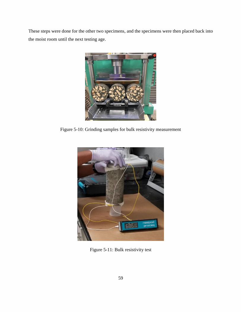
59

These steps were done for the other two specimens, and the specimens were then placed back into

the moist room until the next testing age.

Figure 5-10: Grinding samples for bulk resistivity measurement

Figure 5-11: Bulk resistivity test

60

5.2.3 Rapid Chloride Permeability Test

Concrete samples were measured according to ASTM C1202 “Standard Test Method for Electrical

Indication of Concrete's Ability to Resist Chloride Ion Penetration” [3]. This test method is meant

to provide a relatively quick indication of the concrete specimen’s resistance to the penetration of

chloride ions.

Sample preparation was performed over the two days prior to testing. On the first day, the samples

were removed from the moist room and cut into 3 slices that were each 2 in. (50 mm) thick, making

sure that ¼ in. (5 mm) of the top surface was removed. The samples were kept saturated during

the cutting time. The vacuum saturation process began the day before testing. The specimens were

placed in a vacuum desiccator with both ends exposed. The desiccator was then sealed and

connected to a vacuum pump. The vacuum was maintained for three hours in the desiccator. After

that, the desiccator was filled with de-aired water until the specimens were submerged while the

vacuum pump was still running. The vacuum pump was left running and connected to the

desiccator for an additional hour. The desiccator was then opened and the specimens were left to

soak in the water for 18 ± 2 hours.

After removing the samples from the desiccator, they were placed inside the RCPT test cell,

clamped, and checked to make sure they did not leak. The negative side of the cell was filled with

a 3% NaCl solution, and the positive side of the cell was filled with a 0.3 N NaOH solution. The

positive (red) wire, negative (black) wire, and the thermocouple (to monitor the testing solution

temperature) were connected to the testing cell and the testing unit as shown in Figure 5-12. The

voltage was set to 60 ± 0.1 V, and the test was left running for 6 hours. The current reading was

recorded at the beginning of the test and every 30 minutes thereafter.

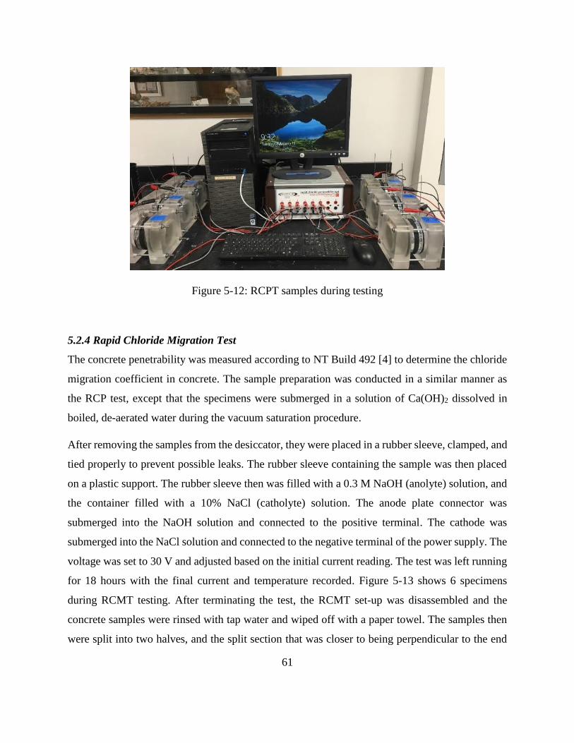
61

Figure 5-12: RCPT samples during testing

5.2.4 Rapid Chloride Migration Test

The concrete penetrability was measured according to NT Build 492 [4] to determine the chloride

migration coefficient in concrete. The sample preparation was conducted in a similar manner as

the RCP test, except that the specimens were submerged in a solution of Ca(OH)2 dissolved in

boiled, de-aerated water during the vacuum saturation procedure.

After removing the samples from the desiccator, they were placed in a rubber sleeve, clamped, and

tied properly to prevent possible leaks. The rubber sleeve containing the sample was then placed

on a plastic support. The rubber sleeve then was filled with a 0.3 M NaOH (anolyte) solution, and

the container filled with a 10% NaCl (catholyte) solution. The anode plate connector was

submerged into the NaOH solution and connected to the positive terminal. The cathode was

submerged into the NaCl solution and connected to the negative terminal of the power supply. The

voltage was set to 30 V and adjusted based on the initial current reading. The test was left running

for 18 hours with the final current and temperature recorded. Figure 5-13 shows 6 specimens

during RCMT testing. After terminating the test, the RCMT set-up was disassembled and the

concrete samples were rinsed with tap water and wiped off with a paper towel. The samples then

were split into two halves, and the split section that was closer to being perpendicular to the end

62

surfaces was sprayed with 0.1 M silver nitrate. Approximately 20 minutes after spraying the

specimens, the penetration depth of chlorides was then measured from the center to both edges at

intervals of 10 mm, at an accuracy of 0.1 mm, with a slide caliper as shown in Figure 5-14. A total

of eight readings were then averaged to get the relative depth of chloride penetration for each

specimen.

Figure 5-13: RCMT during testing

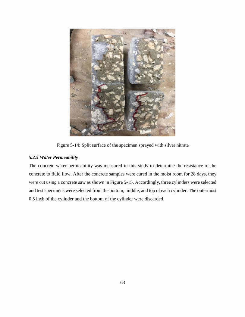
63

Figure 5-14: Split surface of the specimen sprayed with silver nitrate

5.2.5 Water Permeability

The concrete water permeability was measured in this study to determine the resistance of the

concrete to fluid flow. After the concrete samples were cured in the moist room for 28 days, they

were cut using a concrete saw as shown in Figure 5-15. Accordingly, three cylinders were selected

and test specimens were selected from the bottom, middle, and top of each cylinder. The outermost

0.5 inch of the cylinder and the bottom of the cylinder were discarded.

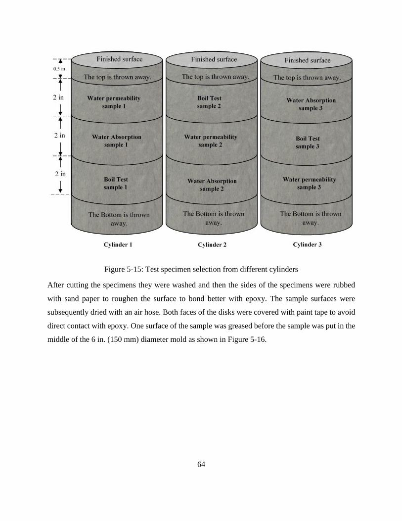
64

Figure 5-15: Test specimen selection from different cylinders

After cutting the specimens they were washed and then the sides of the specimens were rubbed

with sand paper to roughen the surface to bond better with epoxy. The sample surfaces were

subsequently dried with an air hose. Both faces of the disks were covered with paint tape to avoid

direct contact with epoxy. One surface of the sample was greased before the sample was put in the

middle of the 6 in. (150 mm) diameter mold as shown in Figure 5-16.

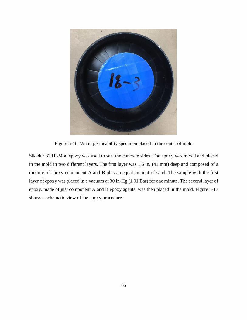
65

Figure 5-16: Water permeability specimen placed in the center of mold

Sikadur 32 Hi-Mod epoxy was used to seal the concrete sides. The epoxy was mixed and placed

in the mold in two different layers. The first layer was 1.6 in. (41 mm) deep and composed of a

mixture of epoxy component A and B plus an equal amount of sand. The sample with the first

layer of epoxy was placed in a vacuum at 30 in-Hg (1.01 Bar) for one minute. The second layer of

epoxy, made of just component A and B epoxy agents, was then placed in the mold. Figure 5-17

shows a schematic view of the epoxy procedure.

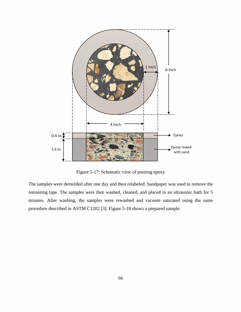
66

Figure 5-17: Schematic view of pouring epoxy

The samples were demolded after one day and then relabeled. Sandpaper was used to remove the

remaining tape. The samples were then washed, cleaned, and placed in an ultrasonic bath for 5

minutes. After washing, the samples were rewashed and vacuum saturated using the same

procedure described in ASTM C1202 [3]. Figure 5-18 shows a prepared sample.

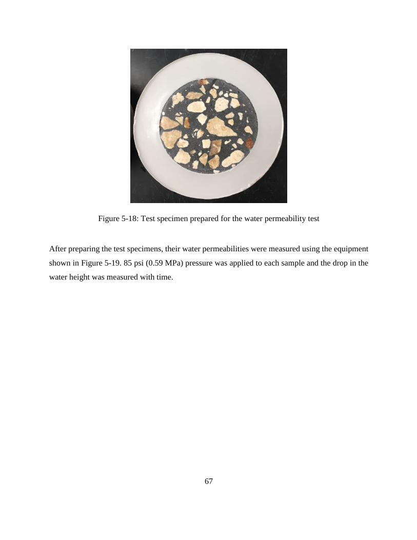
67

Figure 5-18: Test specimen prepared for the water permeability test

After preparing the test specimens, their water permeabilities were measured using the equipment

shown in Figure 5-19. 85 psi (0.59 MPa) pressure was applied to each sample and the drop in the

water height was measured with time.

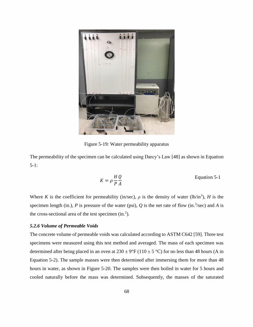
68

Figure 5-19: Water permeability apparatus

The permeability of the specimen can be calculated using Darcy’s Law [48] as shown in Equation

5-1:

𝐾 = 𝜌𝐻

𝑃

𝑄

𝐴

Equation 5-1

Where K is the coefficient for permeability (in/sec), ρ is the density of water (lb/in3), H is the

specimen length (in.), P is pressure of the water (psi), Q is the net rate of flow (in.3/sec) and A is

the cross-sectional area of the test specimen (in.2).

5.2.6 Volume of Permeable Voids

The concrete volume of permeable voids was calculated according to ASTM C642 [59]. Three test

specimens were measured using this test method and averaged. The mass of each specimen was

determined after being placed in an oven at 230 ± 9°F (110 ± 5 °C) for no less than 48 hours (A in

Equation 5-2). The sample masses were then determined after immersing them for more than 48

hours in water, as shown in Figure 5-20. The samples were then boiled in water for 5 hours and

cooled naturally before the mass was determined. Subsequently, the masses of the saturated

69

samples were measured while suspended in water (D), and then the masses of the saturated samples

were measured after the surfaces were towel-dried (C).

Figure 5-20: Immersion of sample in water

The volume of permeable voids can be calculated using Equation 5-2:

𝑉𝑜𝑙𝑢𝑚𝑒 𝑜𝑓 𝑝𝑒𝑟𝑚𝑒𝑎𝑏𝑙𝑒 𝑝𝑜𝑟𝑒 𝑠𝑝𝑎𝑐𝑒 (𝑣𝑜𝑖𝑑𝑠 %) = 𝐶 − 𝐴

𝐶 − 𝐷× 100 Equation 5-2

where A is mass of the oven-dried sample in air (g), C is mass of surface-dry sample in air after

immersion and boiling (g) and D is apparent mass of sample suspended in water after immersion

and boiling (g).

5.2.7 Water Absorption

The water absorption of concrete mixtures was measured according to ASTM C1585 “Standard

Test Method for Measurement of Rate of Absorption of Water by Hydraulic-Cement Concretes.”

[9] This test measures the concrete’s rate of water absorption due to capillary suction. Three

specimens were placed inside an oven at 122 ± 3.6°F (50 ± 2°C) for 3 days in a sealed container

where a saturated potassium bromide solution was placed below the samples in the bottom of the

container to control the relative humidity, followed by 15 days at 73 ± 3.6°F (23 ± 2°C) in a

sealable container. The samples were kept in sealable containers with minimum contact to the wall

of the container to allow free flow of air around the specimen, then the top and sides of the

specimens were sealed with plastic sheeting and duct tape. The absorption test was then started by

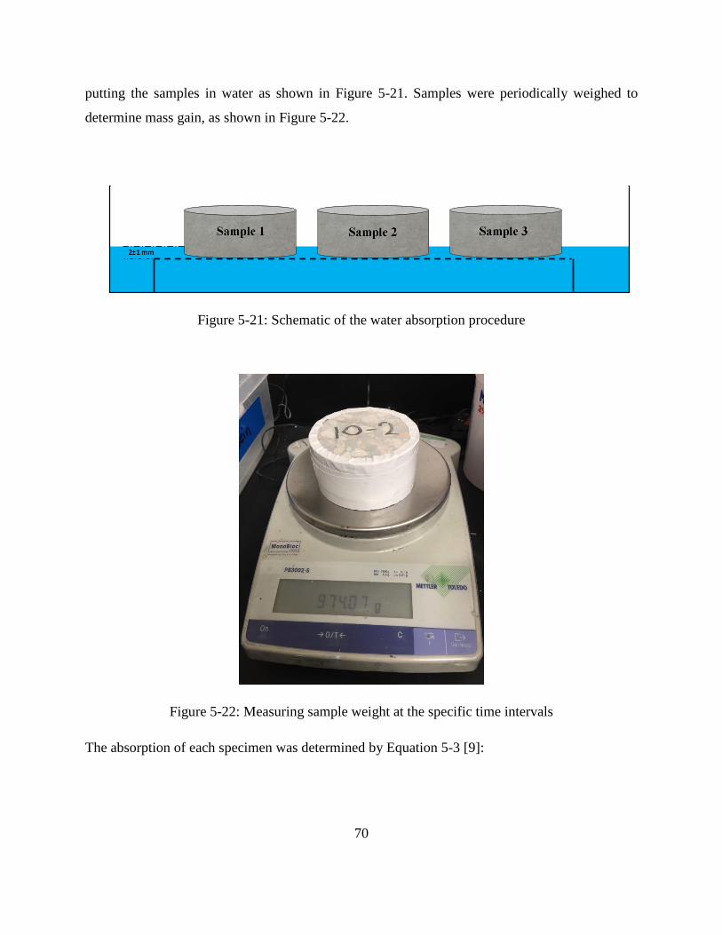
70

putting the samples in water as shown in Figure 5-21. Samples were periodically weighed to

determine mass gain, as shown in Figure 5-22.

Figure 5-21: Schematic of the water absorption procedure

Figure 5-22: Measuring sample weight at the specific time intervals

The absorption of each specimen was determined by Equation 5-3 [9]:

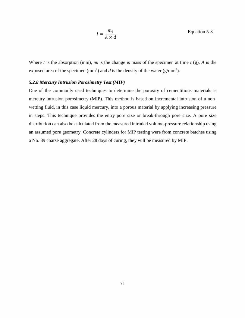
71

𝐼 =𝑚𝑡

𝐴 × 𝑑

Equation 5-3

Where I is the absorption (mm), mt is the change is mass of the specimen at time t (g), A is the

exposed area of the specimen (mm2) and d is the density of the water (g/mm3).

5.2.8 Mercury Intrusion Porosimetry Test (MIP)

One of the commonly used techniques to determine the porosity of cementitious materials is

mercury intrusion porosimetry (MIP). This method is based on incremental intrusion of a non-

wetting fluid, in this case liquid mercury, into a porous material by applying increasing pressure

in steps. This technique provides the entry pore size or break-through pore size. A pore size

distribution can also be calculated from the measured intruded volume-pressure relationship using

an assumed pore geometry. Concrete cylinders for MIP testing were from concrete batches using

a No. 89 coarse aggregate. After 28 days of curing, they will be measured by MIP.

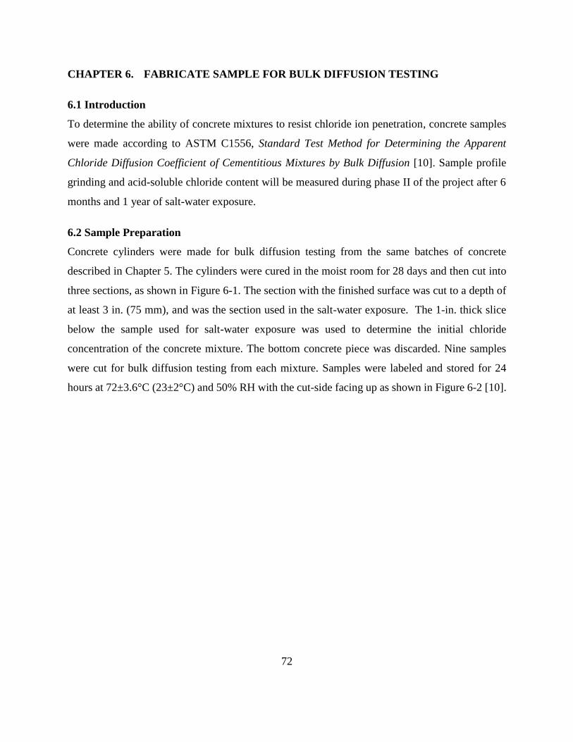
72

CHAPTER 6. FABRICATE SAMPLE FOR BULK DIFFUSION TESTING

6.1 Introduction

To determine the ability of concrete mixtures to resist chloride ion penetration, concrete samples

were made according to ASTM C1556, Standard Test Method for Determining the Apparent

Chloride Diffusion Coefficient of Cementitious Mixtures by Bulk Diffusion [10]. Sample profile

grinding and acid-soluble chloride content will be measured during phase II of the project after 6

months and 1 year of salt-water exposure.

6.2 Sample Preparation

Concrete cylinders were made for bulk diffusion testing from the same batches of concrete

described in Chapter 5. The cylinders were cured in the moist room for 28 days and then cut into

three sections, as shown in Figure 6-1. The section with the finished surface was cut to a depth of

at least 3 in. (75 mm), and was the section used in the salt-water exposure. The 1-in. thick slice

below the sample used for salt-water exposure was used to determine the initial chloride

concentration of the concrete mixture. The bottom concrete piece was discarded. Nine samples

were cut for bulk diffusion testing from each mixture. Samples were labeled and stored for 24

hours at 72±3.6°C (23±2°C) and 50% RH with the cut-side facing up as shown in Figure 6-2 [10].

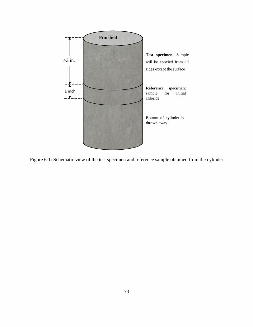
73

Figure 6-1: Schematic view of the test specimen and reference sample obtained from the cylinder

Finished

>3 in.

1 inch

Test specimen: Sample

will be epoxied from all

sides except the surface

Reference specimen:

sample for initial

chloride

Bottom of cylinder is

thrown away.

74

Figure 6-2: Bulk diffusion samples during storage at 23±2ºC and 50% RH

6.3 Epoxy Coating

After the concrete surfaces were dry, the bottom and sides of each sample were sealed with epoxy

to force one-dimensional chloride ingress through the finished surface. A two-component epoxy

(Sikadur 32 Hi-Mod) was used as the sealant. To mix the epoxy, component B was shaken in a

paint shaker for 5 minutes prior to use. Equal volumes of the A and B components were mixed for

3 minutes before coating the sample sides and bottom. After five hours, the specimens were coated

with a second layer of epoxy. The epoxied samples were then cured overnight.

6.4 Calcium Hydroxide Bath

The epoxied specimens were immersed in a saturated calcium hydroxide water bath for 48 hours

prior to chloride exposure. The samples were soaked in the calcium hydroxide solution to reduce

the effects of absorption on chloride ingress.

6.5 Exposure Condition

After the calcium hydroxide soak period was finished, the samples were rinsed with tap water and

placed in tanks containing 16.5% of sodium chloride (NaCl) at the Florida Department of

75

Transportation (FDOT) State Materials Office (SMO), as shown in Figure 6-3. The chloride

solution is circulated throughout the tank to ensure uniform chloride concentration and exposure

for all samples. Figure 6-4 illustrates the sample placement in the tank.

Figure 6-3: Tank containing 16.5% NaCl solution and bulk diffusion samples

Figure 6-4: One-dimensional chloride ingress in the tank

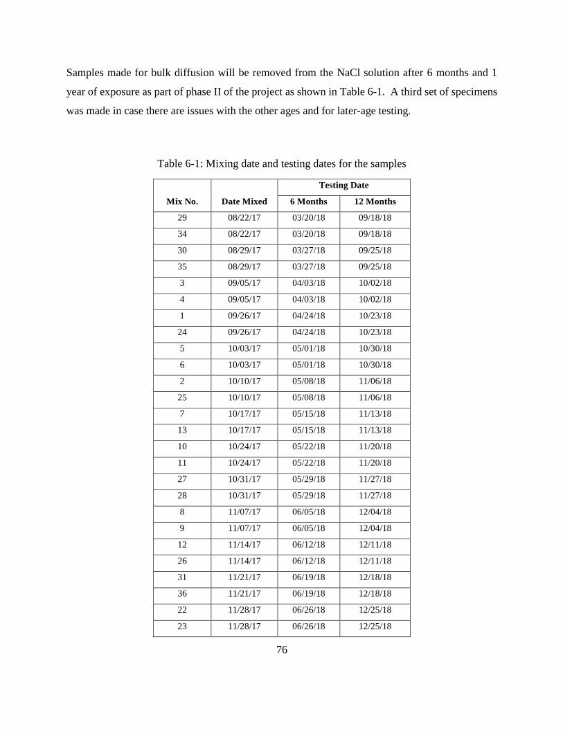
76

Samples made for bulk diffusion will be removed from the NaCl solution after 6 months and 1

year of exposure as part of phase II of the project as shown in Table 6-1. A third set of specimens

was made in case there are issues with the other ages and for later-age testing.

Table 6-1: Mixing date and testing dates for the samples

Mix No. Date Mixed

Testing Date

6 Months 12 Months

29 08/22/17 03/20/18 09/18/18

34 08/22/17 03/20/18 09/18/18

30 08/29/17 03/27/18 09/25/18

35 08/29/17 03/27/18 09/25/18

3 09/05/17 04/03/18 10/02/18

4 09/05/17 04/03/18 10/02/18

1 09/26/17 04/24/18 10/23/18

24 09/26/17 04/24/18 10/23/18

5 10/03/17 05/01/18 10/30/18

6 10/03/17 05/01/18 10/30/18

2 10/10/17 05/08/18 11/06/18

25 10/10/17 05/08/18 11/06/18

7 10/17/17 05/15/18 11/13/18

13 10/17/17 05/15/18 11/13/18

10 10/24/17 05/22/18 11/20/18

11 10/24/17 05/22/18 11/20/18

27 10/31/17 05/29/18 11/27/18

28 10/31/17 05/29/18 11/27/18

8 11/07/17 06/05/18 12/04/18

9 11/07/17 06/05/18 12/04/18

12 11/14/17 06/12/18 12/11/18

26 11/14/17 06/12/18 12/11/18

31 11/21/17 06/19/18 12/18/18

36 11/21/17 06/19/18 12/18/18

22 11/28/17 06/26/18 12/25/18

23 11/28/17 06/26/18 12/25/18

77

Mix No. Date Mixed

Testing Date

6 Months 12 Months

32 12/12/17 07/10/18 01/08/19

37 12/12/17 07/10/18 01/08/19

33 12/19/17 07/17/18 01/15/19

38 12/19/17 07/17/18 01/15/19

17 01/02/18 07/31/18 01/29/19

21 01/02/18 07/31/18 01/29/19

14 01/09/18 08/07/18 02/05/19

15 01/09/18 08/07/18 02/05/19

16 01/16/18 08/14/18 02/12/19

18 01/16/18 08/14/18 02/12/19

19 01/23/18 08/21/18 02/19/19

20 01/23/18 08/21/18 02/19/19

39 01/30/18 08/28/18 02/26/19

40 01/30/18 08/28/18 02/26/19

1 r 2/6/2018 09/04/18 03/05/19

24 r 2/6/2018 09/04/18 03/05/19

78

CHAPTER 7. CHLORIDE BINDING SAMPLE FABRICATION

7.1 Cement Paste Mixtures

Cement paste mixtures were made in order to measure the chloride binding isotherm for the

cementitious material used in each concrete mixture made in this study. The chloride binding

isotherms will be used to separate chloride binding effects from diffusion effects in the chloride

bulk diffusion (ASTM C1556 [10]) samples made in this study. Table 7-1 summarizes the cement

paste mixture proportions that the research team used in studying chloride binding.

Table 7-1: Cement Paste Mixture Proportions

Mix

# Mix ID

Cement (%) SCM Type (%)

w/cm

Type

I/II

Type

V

Type

IL

Type I

HA

Fly

Ash

Slag

Cement

Silica

Fume Metakaolin

1 C-100 100 0.35

2 C-100h 100 0.44

3 C-F10 90 10 0.35

4 C-F20 80 20 0.35

5 C-F10h 90 10 0.44

6 C-F20h 80 20 0.44

7 C-G60 40 60 0.35

8 C-S8 92 8 0.35

9 C-M10 90 10 0.35

10 C-F10G30 60 10 30 0.35

11 C-F10G45 45 10 45 0.35

12 C-F10G60 30 10 60 0.35

13 C-F10G60h 30 10 60 0.44

14 C-F20S4 76 20 4 0.35

15 C-F20S6 74 20 6 0.35

16 C-F20S8 72 20 8 0.35

17 C-F20S8h 72 20 8 0.44

18 C-F20M6 74 20 6 0.35

19 C-F20M8 72 20 8 0.35

20 C-F20M10 70 20 10 0.35

21 C-F20M10h 70 20 10 0.44

22 C-G55S8 37 55 8 0.35

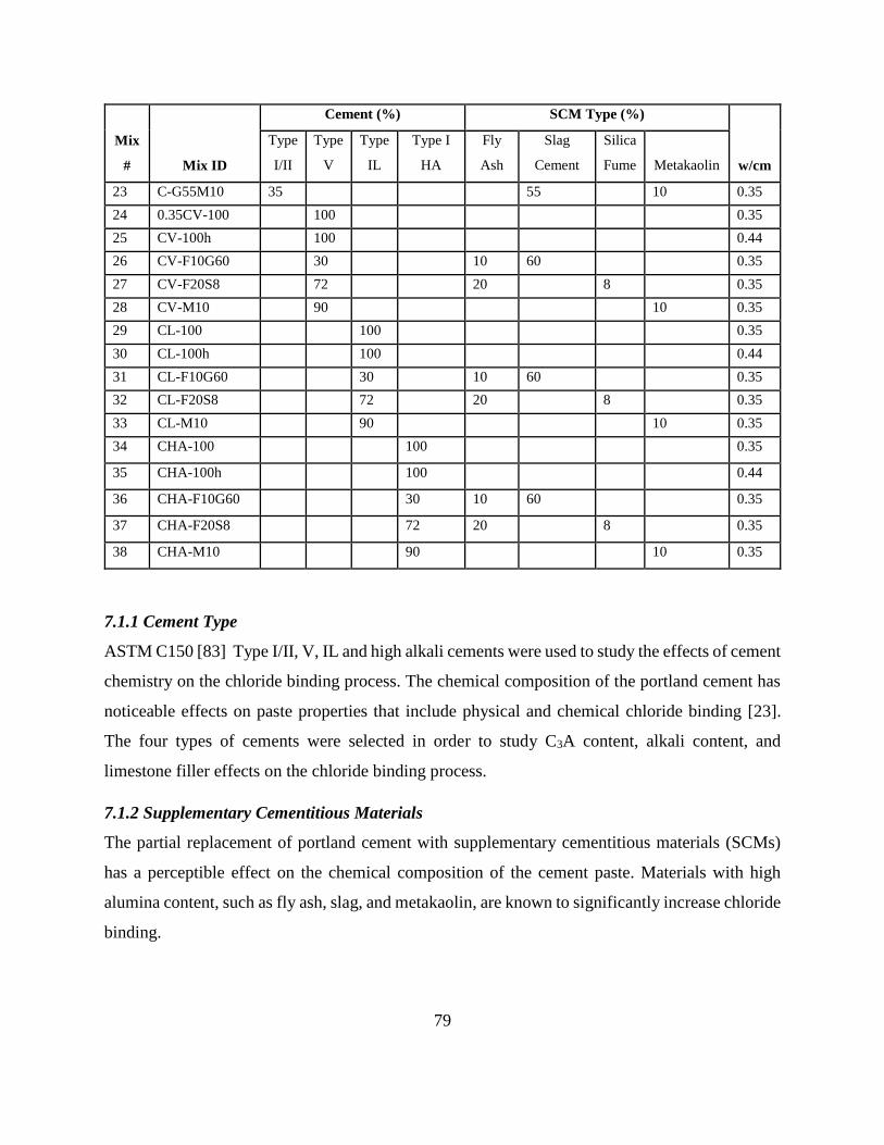
79

Mix

# Mix ID

Cement (%) SCM Type (%)

w/cm

Type

I/II

Type

V

Type

IL

Type I

HA

Fly

Ash

Slag

Cement

Silica

Fume Metakaolin

23 C-G55M10 35 55 10 0.35

24 0.35CV-100 100 0.35

25 CV-100h 100 0.44

26 CV-F10G60 30 10 60 0.35

27 CV-F20S8 72 20 8 0.35

28 CV-M10 90 10 0.35

29 CL-100 100 0.35

30 CL-100h 100 0.44

31 CL-F10G60 30 10 60 0.35

32 CL-F20S8 72 20 8 0.35

33 CL-M10 90 10 0.35

34 CHA-100 100 0.35

35 CHA-100h 100 0.44

36 CHA-F10G60 30 10 60 0.35

37 CHA-F20S8 72 20 8 0.35

38 CHA-M10 90 10 0.35

7.1.1 Cement Type

ASTM C150 [83] Type I/II, V, IL and high alkali cements were used to study the effects of cement

chemistry on the chloride binding process. The chemical composition of the portland cement has

noticeable effects on paste properties that include physical and chemical chloride binding [23].

The four types of cements were selected in order to study C3A content, alkali content, and

limestone filler effects on the chloride binding process.

7.1.2 Supplementary Cementitious Materials

The partial replacement of portland cement with supplementary cementitious materials (SCMs)

has a perceptible effect on the chemical composition of the cement paste. Materials with high

alumina content, such as fly ash, slag, and metakaolin, are known to significantly increase chloride

binding.

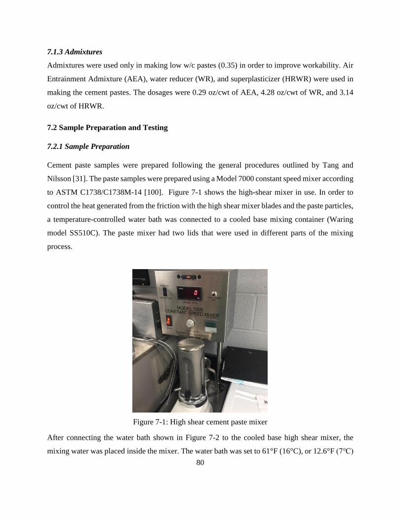
80

7.1.3 Admixtures

Admixtures were used only in making low w/c pastes (0.35) in order to improve workability. Air

Entrainment Admixture (AEA), water reducer (WR), and superplasticizer (HRWR) were used in

making the cement pastes. The dosages were 0.29 oz/cwt of AEA, 4.28 oz/cwt of WR, and 3.14

oz/cwt of HRWR.

7.2 Sample Preparation and Testing

7.2.1 Sample Preparation

Cement paste samples were prepared following the general procedures outlined by Tang and

Nilsson [31]. The paste samples were prepared using a Model 7000 constant speed mixer according

to ASTM C1738/C1738M-14 [100]. Figure 7-1 shows the high-shear mixer in use. In order to

control the heat generated from the friction with the high shear mixer blades and the paste particles,

a temperature-controlled water bath was connected to a cooled base mixing container (Waring

model SS510C). The paste mixer had two lids that were used in different parts of the mixing

process.

Figure 7-1: High shear cement paste mixer

After connecting the water bath shown in Figure 7-2 to the cooled base high shear mixer, the

mixing water was placed inside the mixer. The water bath was set to 61°F (16°C), or 12.6°F (7℃)

81

below the target mixing temperature in order to cool the mixing water. After cooling the mixing

water, the cementitious materials were placed in the mixer through the feeder lid while the mixer

was running at 4000 rpm, shown in Figure 7-3. Uniform distribution of materials was ensured

during material addition and was completed in 60 seconds. After adding the cementitious

materials, the feeder lid was replaced with the high shear lid as shown in Figure 7-1. The paste

was mixed at 10,000 rpm for 30 seconds, followed by a rest period of 150 seconds, and a final

mixing at 10,000 rpm for 30 seconds. During the first 15 seconds of the rest period, the temperature

was checked and the sides of the mixer were scraped using a scraper.

Figure 7-2: Water bath to control the paste temperature.

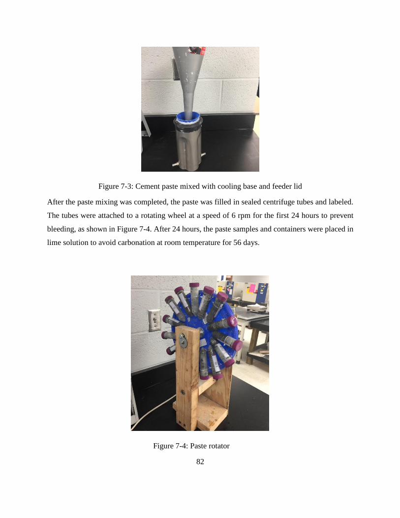
82

Figure 7-3: Cement paste mixed with cooling base and feeder lid

After the paste mixing was completed, the paste was filled in sealed centrifuge tubes and labeled.

The tubes were attached to a rotating wheel at a speed of 6 rpm for the first 24 hours to prevent

bleeding, as shown in Figure 7-4. After 24 hours, the paste samples and containers were placed in

lime solution to avoid carbonation at room temperature for 56 days.

Figure 7-4: Paste rotator

83

7.2.2 Sample Conditioning

After the curing period, the samples were demolded and cut into approximately 3 mm thick disks

using a wafering saw, as shown in Figure 7-5. The disks were vacuum-dried for 3 days.

Figure 7-5: Wavering saw used in cutting the cement paste disks

Paste samples were placed in five different chloride solutions. Approximately 0.88 oz (25 g) of

paste was placed in each container containing 100 mL of solution, as shown in Figure 7-6. Chloride

concentrations of 0.1, 0.3, 0.5, 1.0 and 3.0 M were used. Each solution was additionally saturated

(3 g/L) with calcium hydroxide to reduce leaching. The containers were sealed and stored at room

temperature for 12 weeks, as shown in Figure 7-7.

84

Figure 7-6: Paste samples placed in chloride solution

Figure 7-7: Paste in chloride solution samples for all 38 mixtures

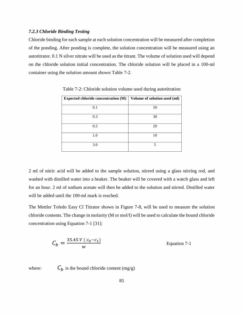
85

7.2.3 Chloride Binding Testing

Chloride binding for each sample at each solution concentration will be measured after completion

of the ponding. After ponding is complete, the solution concentration will be measured using an

autotitrator. 0.1 N silver nitrate will be used as the titrant. The volume of solution used will depend

on the chloride solution initial concentration. The chloride solution will be placed in a 100-ml

container using the solution amount shown Table 7-2.

Table 7-2: Chloride solution volume used during autotitration

Expected chloride concentration (M) Volume of solution used (ml)

0.1 50

0.3 30

0.5 20

1.0 10

3.0 5

2 ml of nitric acid will be added to the sample solution, stirred using a glass stirring rod, and

washed with distilled water into a beaker. The beaker will be covered with a watch glass and left

for an hour. 2 ml of sodium acetate will then be added to the solution and stirred. Distilled water

will be added until the 100-ml mark is reached.

The Mettler Toledo Easy Cl Titrator shown in Figure 7-8, will be used to measure the solution

chloride contents. The change in molarity (M or mol/l) will be used to calculate the bound chloride

concentration using Equation 7-1 [31]:

𝐶𝑏 =35.45 𝑉 ( 𝑐0−𝑐1)

𝑤 Equation 7-1

where: 𝐶𝑏 is the bound chloride content (mg/g)

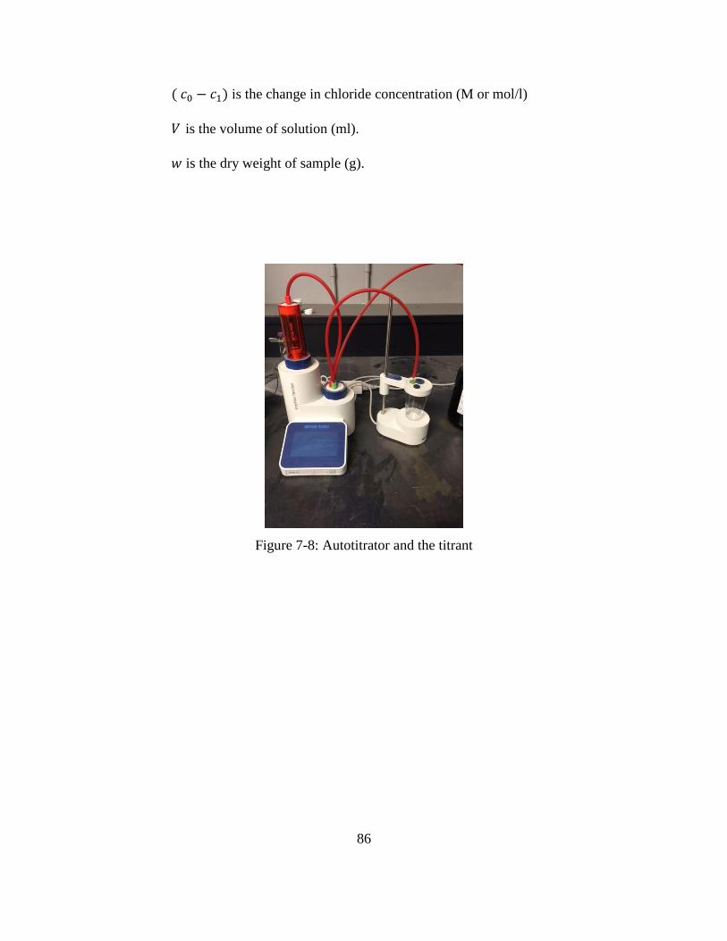
86

( 𝑐0 − 𝑐1) is the change in chloride concentration (M or mol/l)

𝑉 is the volume of solution (ml).

𝑤 is the dry weight of sample (g).

Figure 7-8: Autotitrator and the titrant

87

CHAPTER 8. SULFATE ATTACK SPECIMEN FABRICATION

8.1 Introduction

The durability of concrete mixtures to sulfate attack is being measured in this study. This durability

will be compared to the concrete penetrability measured. The durability of concrete to sulfate

attack is a function both of the ability of the concrete to keep sulfate ions out of the concrete and

the chemical composition of the cementitious materials. The durability of concrete made with two

water-to-cementitious material ratios (w/cm) and several different combinations of supplementary

cementitious materials (SCMs) are being tested during exposure to a 5% sodium sulfate solution.

8.2 Prism Preparation

For every mix, three steel prism molds were assembled with gauge studs attached to each inner

mold end in accordance with ASTM C490 [101]. An example of prism molds ready for use is

shown in Figure 8-1. The steel molds were oiled with 5W-20 motor oil to facilitate concrete

removal. After mixing the concrete following ASTM C192 [94] and measuring the fresh properties

of the mixture, concrete was placed in the molds in two layers, as shown in Figure 8-2.

Figure 8-1: Prism molds assembled and ready for use

88

Figure 8-2: Concrete placement in mold

After the first layer of concrete was placed, the prism mold was vibrated on a vibrating table as

shown in Figure 8-2, after which the second layer was added. The mold was vibrated again and

finished using a trowel as seen in Figure 8-3. Figure 8-4 shows a prism after finishing. The prisms

were demolded after 24 hours and moist cured for 28 days in accordance with the requirements of

ASTM C511 [102], as shown in Figure 8-5 and Figure 8-6.

Figure 8-3: Prism being finished

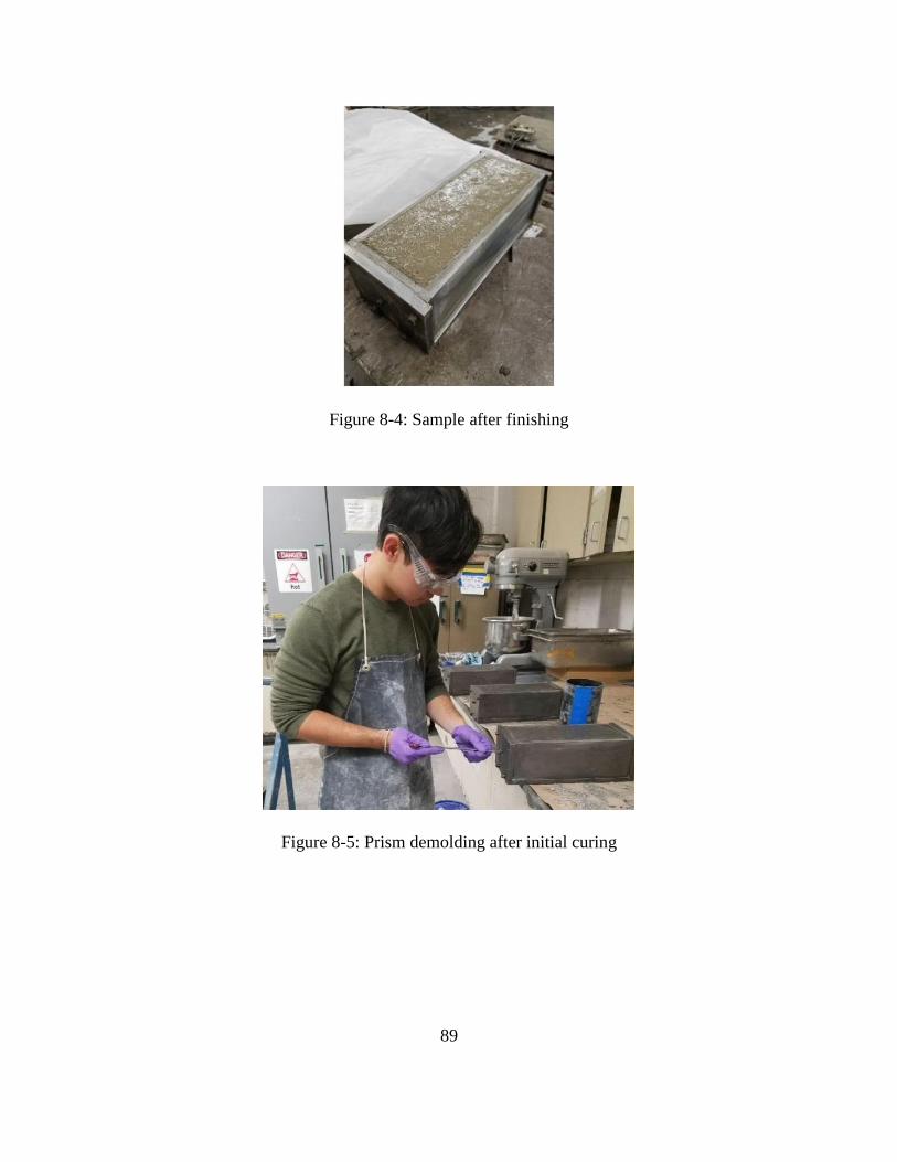
89

Figure 8-4: Sample after finishing

Figure 8-5: Prism demolding after initial curing

90

Figure 8-6: Samples placed in moist curing room for curing prior to sulfate exposure

8.3 Modified ASTM C1012

The purpose of ASTM C1012 “Standard Test Method for Length Change of Hydraulic-Cement

Mortars Exposed to a Sulfate Solution” [103] is to assess the inherent susceptibility of a

cementitious system to sulfate attack by exposure to a 5% sodium sulfate solution. Since ASTM

C1012 does not account for variations in water-cementitious material ratio (w/cm) on the

durability, it was modified to use concrete prisms. Drimalas [19] modified ASTM C1012 to use 3

x 3 x 11.25 in. concrete prisms instead of mortar bars. To accommodate larger aggregates than

used by Drimalas, 4 x 4 x 11.25 in. concrete prisms were used in this study.

After moist curing for 28 days, initial length readings of three prisms from each mix were

measured. As shown in Figure 8-7, the readings were performed using a length change comparator

as specified in ASTM C490. After the initial reading, the three prisms were put in a sealable

container that contained 3.5 to 4.5 times their volumes in a 5% concentration sodium sulfate

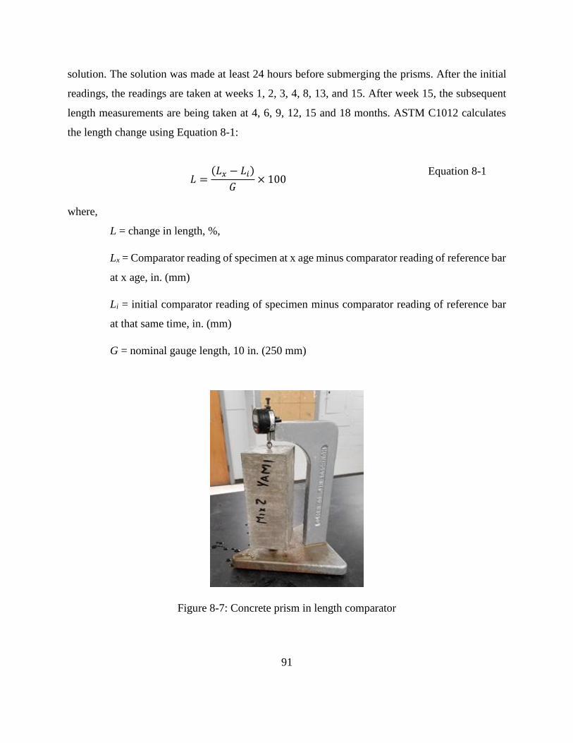
91

solution. The solution was made at least 24 hours before submerging the prisms. After the initial

readings, the readings are taken at weeks 1, 2, 3, 4, 8, 13, and 15. After week 15, the subsequent

length measurements are being taken at 4, 6, 9, 12, 15 and 18 months. ASTM C1012 calculates

the length change using Equation 8-1:

𝐿 =(𝐿𝑥 − 𝐿𝑖)

𝐺× 100

Equation 8-1

where,

L = change in length, %,

Lx = Comparator reading of specimen at x age minus comparator reading of reference bar

at x age, in. (mm)

Li = initial comparator reading of specimen minus comparator reading of reference bar

at that same time, in. (mm)

G = nominal gauge length, 10 in. (250 mm)

Figure 8-7: Concrete prism in length comparator

92

The prisms are placed back in a 5% sodium sulfate solution in a sealed container after every

reading, as shown in Figure 8-8. The solution is replaced with new sodium sulfate solution at the

time of each measurement age.

Figure 8-8: Prisms stored in 5% sodium sulfate solution

8.4 Results to Date

Samples have started their exposure period to the 5% sodium sulfate solution. Table 8-1 shows the

average prism length change of the mixtures tested so far. Sample mixtures are listed in the order

that they were made. Length change measurements will continue and finish during phase II of the

project.

Table 8-1: Preliminary length change readings for concrete prisms exposed to 5% sodium sulfate

solution

Mix No.

Concrete Age (Weeks)

Initial Reading W1 W2 W3 W4 W8 W13 W15 W17

Mix 29 0.000 -0.010 0.000 0.000 -0.004 -0.001 0.000 -0.001 0.001

Mix34 0.000 -0.001 0.005 0.004 0.005 0.006 0.008 0.011 0.011

Mix 30 0.000 0.006 0.006 0.005 0.002 0.006 0.003 0.008 0.007

Mix 35 0.000 0.003 0.004 0.000 0.002 0.008 -0.002 0.010 0.009

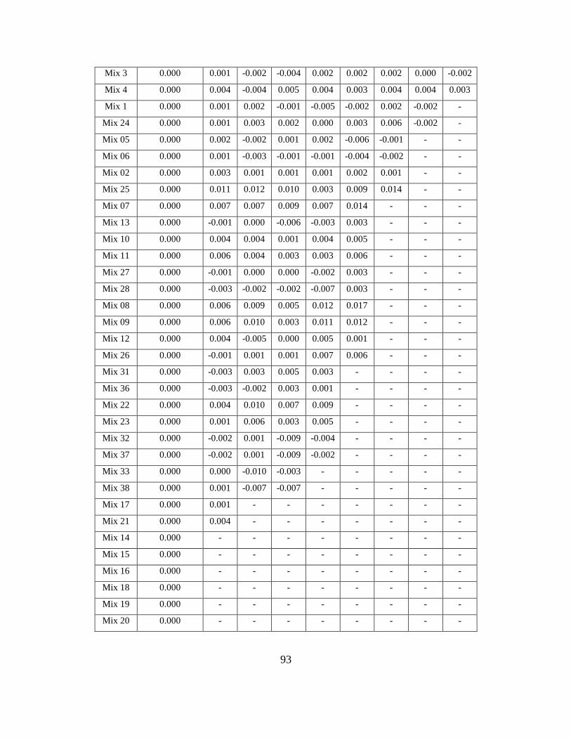
93

Mix 3 0.000 0.001 -0.002 -0.004 0.002 0.002 0.002 0.000 -0.002

Mix 4 0.000 0.004 -0.004 0.005 0.004 0.003 0.004 0.004 0.003

Mix 1 0.000 0.001 0.002 -0.001 -0.005 -0.002 0.002 -0.002 -

Mix 24 0.000 0.001 0.003 0.002 0.000 0.003 0.006 -0.002 -

Mix 05 0.000 0.002 -0.002 0.001 0.002 -0.006 -0.001 - -

Mix 06 0.000 0.001 -0.003 -0.001 -0.001 -0.004 -0.002 - -

Mix 02 0.000 0.003 0.001 0.001 0.001 0.002 0.001 - -

Mix 25 0.000 0.011 0.012 0.010 0.003 0.009 0.014 - -

Mix 07 0.000 0.007 0.007 0.009 0.007 0.014 - - -

Mix 13 0.000 -0.001 0.000 -0.006 -0.003 0.003 - - -

Mix 10 0.000 0.004 0.004 0.001 0.004 0.005 - - -

Mix 11 0.000 0.006 0.004 0.003 0.003 0.006 - - -

Mix 27 0.000 -0.001 0.000 0.000 -0.002 0.003 - - -

Mix 28 0.000 -0.003 -0.002 -0.002 -0.007 0.003 - - -

Mix 08 0.000 0.006 0.009 0.005 0.012 0.017 - - -

Mix 09 0.000 0.006 0.010 0.003 0.011 0.012 - - -

Mix 12 0.000 0.004 -0.005 0.000 0.005 0.001 - - -

Mix 26 0.000 -0.001 0.001 0.001 0.007 0.006 - - -

Mix 31 0.000 -0.003 0.003 0.005 0.003 - - - -

Mix 36 0.000 -0.003 -0.002 0.003 0.001 - - - -

Mix 22 0.000 0.004 0.010 0.007 0.009 - - - -

Mix 23 0.000 0.001 0.006 0.003 0.005 - - - -

Mix 32 0.000 -0.002 0.001 -0.009 -0.004 - - - -

Mix 37 0.000 -0.002 0.001 -0.009 -0.002 - - - -

Mix 33 0.000 0.000 -0.010 -0.003 - - - - -

Mix 38 0.000 0.001 -0.007 -0.007 - - - - -

Mix 17 0.000 0.001 - - - - - - -

Mix 21 0.000 0.004 - - - - - - -

Mix 14 0.000 - - - - - - - -

Mix 15 0.000 - - - - - - - -

Mix 16 0.000 - - - - - - - -

Mix 18 0.000 - - - - - - - -

Mix 19 0.000 - - - - - - - -

Mix 20 0.000 - - - - - - - -

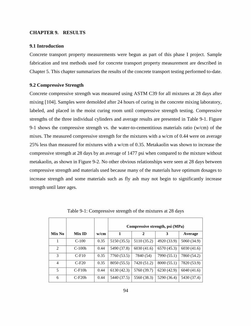
94

CHAPTER 9. RESULTS

9.1 Introduction

Concrete transport property measurements were begun as part of this phase I project. Sample

fabrication and test methods used for concrete transport property measurement are described in

Chapter 5. This chapter summarizes the results of the concrete transport testing performed to-date.

9.2 Compressive Strength

Concrete compressive strength was measured using ASTM C39 for all mixtures at 28 days after

mixing [104]. Samples were demolded after 24 hours of curing in the concrete mixing laboratory,

labeled, and placed in the moist curing room until compressive strength testing. Compressive

strengths of the three individual cylinders and average results are presented in Table 9-1. Figure

9-1 shows the compressive strength vs. the water-to-cementitious materials ratio (w/cm) of the

mixes. The measured compressive strength for the mixtures with a w/cm of 0.44 were on average

25% less than measured for mixtures with a w/cm of 0.35. Metakaolin was shown to increase the

compressive strength at 28 days by an average of 1477 psi when compared to the mixture without

metakaolin, as shown in Figure 9-2. No other obvious relationships were seen at 28 days between

compressive strength and materials used because many of the materials have optimum dosages to

increase strength and some materials such as fly ash may not begin to significantly increase

strength until later ages.

Table 9-1: Compressive strength of the mixtures at 28 days

Mix No Mix ID w/cm

Compressive strength, psi (MPa)

1 2 3 Average

1 C-100 0.35 5150 (35.5) 5110 (35.2) 4920 (33.9) 5060 (34.9)

2 C-100h 0.44 5490 (37.8) 6030 (41.6) 6570 (45.3) 6030 (41.6)

3 C-F10 0.35 7760 (53.5) 7840 (54) 7990 (55.1) 7860 (54.2)

4 C-F20 0.35 8050 (55.5) 7420 (51.2) 8000 (55.1) 7820 (53.9)

5 C-F10h 0.44 6130 (42.3) 5760 (39.7) 6230 (42.9) 6040 (41.6)

6 C-F20h 0.44 5440 (37.5) 5560 (38.3) 5290 (36.4) 5430 (37.4)

95

7 C-G60 0.35 9170 (63.3) 9140 (63) 9180 (63.3) 9160 (63.2)

8 C-S8 0.35 8190 (56.5) 8370 (57.7) 8060 (55.6) 8200 (56.6)

9 C-M10 0.35 9460 (65.2) 8920 (61.5) 7990 (55.1) 8790 (60.6)

10 C-F10G30 0.35 8310 (57.3) 8060 (55.6) 7000 (48.2) 7790 (53.7)

11 C-F10G45 0.35 7680 (53) 8440 (58.2) 7880 (54.3) 8000 (55.2)

12 C-F10G60 0.35 7620 (52.5) 8380 (57.8) 7790 (53.7) 7930 (54.7)

13 C-F10G60h 0.44 6300 (43.4) 6290 (43.4) 6310 (43.5) 6300 (43.5)

14 C-F20S4 0.35 8800 (60.7) 7770 (53.6) 7570 (52.2) 8050 (55.5)

15 C-F20S6 0.35 8530 (58.8) 8890 (61.3) 7040 (48.5) 8160 (56.2)

16 C-F20S8 0.35 8630 (59.5) 7910 (54.6) 7610 (52.5) 8050 (55.5)

17 C-F20S8h 0.44 5930 (40.9) 7070 (48.7) 6440 (44.4) 6480 (44.7)

18 C-F20M6 0.35 7980 (55.1) 8810 (60.7) 8900 (61.4) 8560 (59)

19 C-F20M8 0.35 9190 (63.3) 7540 (52) 9550 (65.9) 8760 (60.4)

20 C-F20M10 0.35 9160 (63.2) 8880 (61.2) 9690 (66.8) 9240 (63.7)

21 C-F20M10h 0.44 5950 (41) 7380 (50.9) 7030 (48.5) 6790 (46.8)

22 C-G55S8 0.35 7600 (52.4) 9070 (62.6) 8950 (61.7) 8540 (58.9)

23 C-G55M10 0.35 8480 (58.5) 8500 (58.6) 7800 (53.8) 8260 (57)

24 CV-100 0.35 7380 (50.9) 8400 (57.9) 8000 (55.2) 7930 (54.7)

25 CV-100h 0.44 6540 (45.1) 6600 (45.5) 6460 (44.5) 6530 (45)

26 CV-F10G60 0.35 8390 (57.8) 7280 (50.2) 8070 (55.6) 7910 (54.6)

27 CV-F20S8 0.35 6890 (47.5) 7300 (50.3) 6190 (42.7) 6790 (46.8)

28 CV-M10 0.35 9010 (62.1) 9530 (65.7) 8580 (59.2) 9040 (62.3)

29 CL-100 0.35 7200 (49.6) 8200 (56.5) 8260 (56.9) 7890 (54.4)

30 CL-100h 0.44 5920 (40.8) 6390 (44.1) 6720 (46.4) 6350 (43.8)

31 CL-F10G60 0.35 7070 (48.7) 7680 (52.9) 6870 (47.4) 7200 (49.7)

32 CL-F20S8 0.35 6860 (47.3) 7600 (52.4) 8360 (57.6) 7600 (52.4)

33 CL-M10 0.35 8710 (60) 9640 (66.5) 9670 (66.7) 9340 (64.4)

34 CHA-100 0.35 6690 (46.1) 6260 (43.2) 6440 (44.4) 6460 (44.6)

35 CHA-100h 0.44 4430 (30.6) 5900 (40.7) 5380 (37.1) 5240 (36.1)

36 CHA-F10G60 0.35 7680 (52.9) 6110 (42.1) 8290 (57.1) 7360 (50.7)

37 CHA-F20S8 0.35 6700 (46.2) 5820 (40.1) 6870 (47.3) 6460 (44.5)

38 CHA-M10 0.35 7640 (52.6) 6760 (46.6) 8190 (56.5) 7530 (51.9)

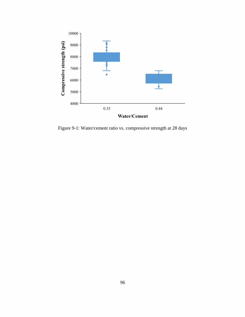
96

Figure 9-1: Water/cement ratio vs. compressive strength at 28 days

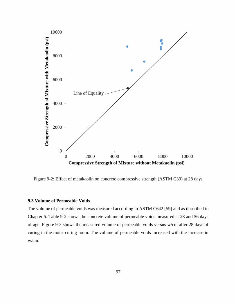
97

Figure 9-2: Effect of metakaolin on concrete compressive strength (ASTM C39) at 28 days

9.3 Volume of Permeable Voids

The volume of permeable voids was measured according to ASTM C642 [59] and as described in

Chapter 5. Table 9-2 shows the concrete volume of permeable voids measured at 28 and 56 days

of age. Figure 9-3 shows the measured volume of permeable voids versus w/cm after 28 days of

curing in the moist curing room. The volume of permeable voids increased with the increase in

w/cm.

0

2000

4000

6000

8000

10000

0 2000 4000 6000 8000 10000

Com

pre

ssiv

e S

tren

gth

of

Mix

ture

wit

h M

etak

aoli

n (

psi

)

Compressive Strength of Mixture without Metakaolin (psi)

Line of Equality

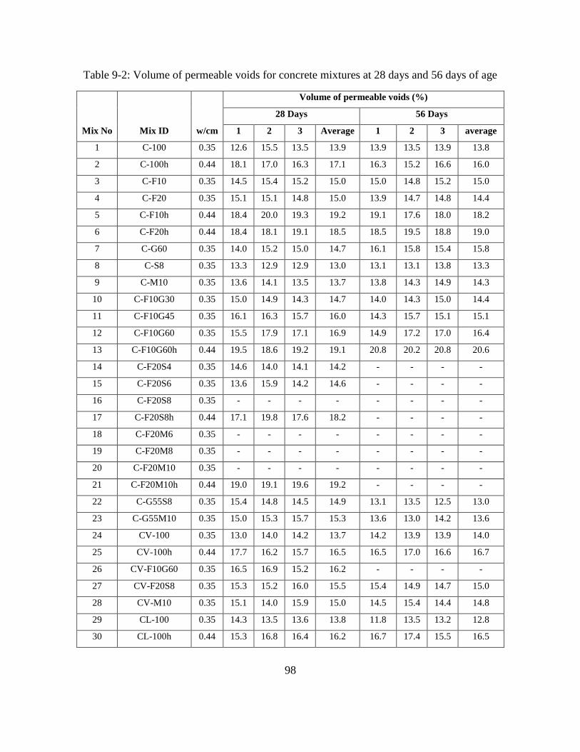
98

Table 9-2: Volume of permeable voids for concrete mixtures at 28 days and 56 days of age

Mix No Mix ID w/cm

Volume of permeable voids (%)

28 Days 56 Days

1 2 3 Average 1 2 3 average

1 C-100 0.35 12.6 15.5 13.5 13.9 13.9 13.5 13.9 13.8

2 C-100h 0.44 18.1 17.0 16.3 17.1 16.3 15.2 16.6 16.0

3 C-F10 0.35 14.5 15.4 15.2 15.0 15.0 14.8 15.2 15.0

4 C-F20 0.35 15.1 15.1 14.8 15.0 13.9 14.7 14.8 14.4

5 C-F10h 0.44 18.4 20.0 19.3 19.2 19.1 17.6 18.0 18.2

6 C-F20h 0.44 18.4 18.1 19.1 18.5 18.5 19.5 18.8 19.0

7 C-G60 0.35 14.0 15.2 15.0 14.7 16.1 15.8 15.4 15.8

8 C-S8 0.35 13.3 12.9 12.9 13.0 13.1 13.1 13.8 13.3

9 C-M10 0.35 13.6 14.1 13.5 13.7 13.8 14.3 14.9 14.3

10 C-F10G30 0.35 15.0 14.9 14.3 14.7 14.0 14.3 15.0 14.4

11 C-F10G45 0.35 16.1 16.3 15.7 16.0 14.3 15.7 15.1 15.1

12 C-F10G60 0.35 15.5 17.9 17.1 16.9 14.9 17.2 17.0 16.4

13 C-F10G60h 0.44 19.5 18.6 19.2 19.1 20.8 20.2 20.8 20.6

14 C-F20S4 0.35 14.6 14.0 14.1 14.2 - - - -

15 C-F20S6 0.35 13.6 15.9 14.2 14.6 - - - -

16 C-F20S8 0.35 - - - - - - - -

17 C-F20S8h 0.44 17.1 19.8 17.6 18.2 - - - -

18 C-F20M6 0.35 - - - - - - - -

19 C-F20M8 0.35 - - - - - - - -

20 C-F20M10 0.35 - - - - - - - -

21 C-F20M10h 0.44 19.0 19.1 19.6 19.2 - - - -

22 C-G55S8 0.35 15.4 14.8 14.5 14.9 13.1 13.5 12.5 13.0

23 C-G55M10 0.35 15.0 15.3 15.7 15.3 13.6 13.0 14.2 13.6

24 CV-100 0.35 13.0 14.0 14.2 13.7 14.2 13.9 13.9 14.0

25 CV-100h 0.44 17.7 16.2 15.7 16.5 16.5 17.0 16.6 16.7

26 CV-F10G60 0.35 16.5 16.9 15.2 16.2 - - - -

27 CV-F20S8 0.35 15.3 15.2 16.0 15.5 15.4 14.9 14.7 15.0

28 CV-M10 0.35 15.1 14.0 15.9 15.0 14.5 15.4 14.4 14.8

29 CL-100 0.35 14.3 13.5 13.6 13.8 11.8 13.5 13.2 12.8

30 CL-100h 0.44 15.3 16.8 16.4 16.2 16.7 17.4 15.5 16.5

99

Mix No Mix ID w/cm

Volume of permeable voids (%)

28 Days 56 Days

1 2 3 Average 1 2 3 average

31 CL-F10G60 0.35 17.0 17.4 16.8 17.1 16.5 17.6 17.2 17.1

32 CL-F20S8 0.35 15.2 15.4 15.4 15.3 15.1 15.8 15.2 15.4

33 CL-M10 0.35 13.6 13.5 14.3 13.8 - - - -

34 CHA-100 0.35 16.2 15.9 16.1 16.1 15.3 14.4 14.7 14.8

35 CHA-100h 0.44 18.0 18.5 17.2 17.9 17.1 23.7 17.5 19.4

36 CHA-F10G60 0.35 17.0 17.3 17.5 17.3 17.6 16.2 16.6 16.8

37 CHA-F20S8 0.35 15.6 16.3 16.9 16.3 17.4 16.6 16.6 16.9

38 CHA-M10 0.35 15.4 15.7 16.3 15.8 - - - -

Note: Dash shown in tables represent samples that have not yet reached the age required for

testing or are still being tested

Figure 9-3: Water/cement ratio vs. volume of permeable voids at 28 days

9.4 Water Absorption

Concrete mixtures were made and tested for water absorption according to ASTM C1585 [9].

The initial and secondary absorption rates for tests beginning at 28 and 56 days after concrete

mixing are presented in Table 9-3.

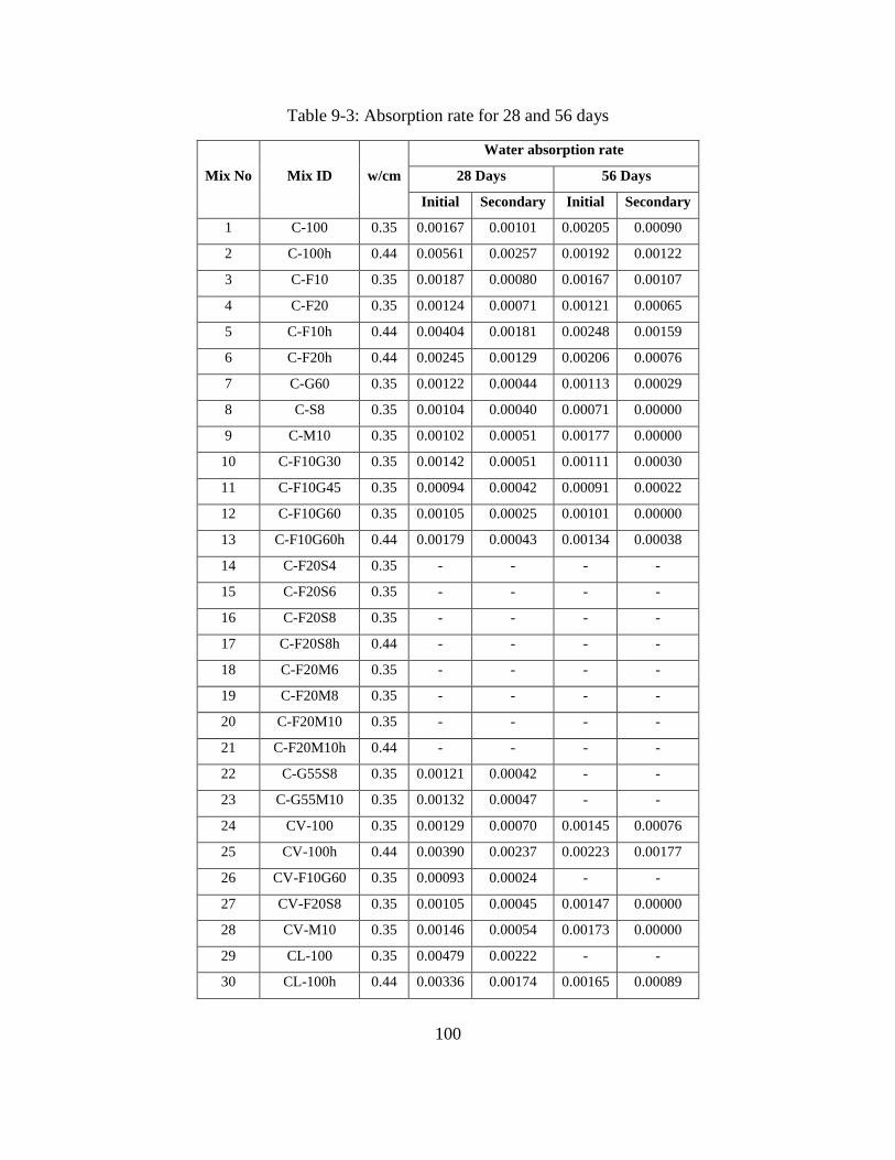
100

Table 9-3: Absorption rate for 28 and 56 days

Mix No Mix ID w/cm

Water absorption rate

28 Days 56 Days

Initial Secondary Initial Secondary

1 C-100 0.35 0.00167 0.00101 0.00205 0.00090

2 C-100h 0.44 0.00561 0.00257 0.00192 0.00122

3 C-F10 0.35 0.00187 0.00080 0.00167 0.00107

4 C-F20 0.35 0.00124 0.00071 0.00121 0.00065

5 C-F10h 0.44 0.00404 0.00181 0.00248 0.00159

6 C-F20h 0.44 0.00245 0.00129 0.00206 0.00076

7 C-G60 0.35 0.00122 0.00044 0.00113 0.00029

8 C-S8 0.35 0.00104 0.00040 0.00071 0.00000

9 C-M10 0.35 0.00102 0.00051 0.00177 0.00000

10 C-F10G30 0.35 0.00142 0.00051 0.00111 0.00030

11 C-F10G45 0.35 0.00094 0.00042 0.00091 0.00022

12 C-F10G60 0.35 0.00105 0.00025 0.00101 0.00000

13 C-F10G60h 0.44 0.00179 0.00043 0.00134 0.00038

14 C-F20S4 0.35 - - - -

15 C-F20S6 0.35 - - - -

16 C-F20S8 0.35 - - - -

17 C-F20S8h 0.44 - - - -

18 C-F20M6 0.35 - - - -

19 C-F20M8 0.35 - - - -

20 C-F20M10 0.35 - - - -

21 C-F20M10h 0.44 - - - -

22 C-G55S8 0.35 0.00121 0.00042 - -

23 C-G55M10 0.35 0.00132 0.00047 - -

24 CV-100 0.35 0.00129 0.00070 0.00145 0.00076

25 CV-100h 0.44 0.00390 0.00237 0.00223 0.00177

26 CV-F10G60 0.35 0.00093 0.00024 - -

27 CV-F20S8 0.35 0.00105 0.00045 0.00147 0.00000

28 CV-M10 0.35 0.00146 0.00054 0.00173 0.00000

29 CL-100 0.35 0.00479 0.00222 - -

30 CL-100h 0.44 0.00336 0.00174 0.00165 0.00089

101

31 CL-F10G60 0.35 0.00105 0.00020 - -

32 CL-F20S8 0.35 - - - -

33 CL-M10 0.35 - - - -

34 CHA-100 0.35 0.00407 0.00150 0.00198 0.00101

35 CHA-100h 0.44 0.00368 0.00165 0.00157 0.00099

36 CHA-F10G60 0.35 0.00156 0.00040 - -

37 CHA-F20S8 0.35 - - - -

38 CHA-M10 0.35 - - - -

9.5 Water Permeability

Concrete samples were made and tested for water permeability as described in Chapter 5. Table 9-

4 shows the water permeability results of the concrete mixtures at 28 and 56 days of age. Figure

9-4 shows the water permeability grouped by w/cm. The higher w/cm resulted in much more

variability in water permeability, probably because of a more connected microstructure.

Table 9-4: Permeability results

Mix No Mix ID w/cm

Permeability

(m/s) – 28 days

(x10-13)

Permeability

(m/s) – 56 days

(x10-13)

1 C-100 0.35 79.0 51.3

2 C-100h 0.44 83.1 73.2

3 C-F10 0.35 38.8 23.1

4 C-F20 0.35 35.7 17.2

5 C-F10h 0.44 19.0 72.3

6 C-F20h 0.44 19.0 67.9

7 C-G60 0.35 8.8 9.1

8 C-S8 0.35 13.3 16.0

9 C-M10 0.35 22.9 29.0

10 C-F10G30 0.35 12.0 12.0

11 C-F10G45 0.35 8.1 5.3

12 C-F10G60 0.35 - -

13 C-F10G60h 0.44 16.6 -

14 C-F20S4 0.35 - -

102

15 C-F20S6 0.35 - -

16 C-F20S8 0.35 - -

17 C-F20S8h 0.44 21.9 -

18 C-F20M6 0.35 - -

19 C-F20M8 0.35 - -

20 C-F20M10 0.35 - -

21 C-F20M10h 0.44 15.9 -

22 C-G55S8 0.35 11.2 -

23 C-G55M10 0.35 9.4 -

24 CV-100 0.35 - -

25 CV-100h 0.44 85.7 -

26 CV-F10G60 0.35 6.8 -

27 CV-F20S8 0.35 28.5 27.6

28 CV-M10 0.35 16.6 16.1

29 CL-100 0.35 30.0 -

30 CL-100h 0.44 47.0 -

31 CL-F10G60 0.35 6.5 13.1

32 CL-F20S8 0.35 - -

33 CL-M10 0.35 - -

34 CHA-100 0.35 - -

35 CHA-100h 0.44 49.0 -

36 CHA-F10G60 0.35 11.0 9.7

37 CHA-F20S8 0.35 14.1 -

38 CHA-M10 0.35 - -

103

Figure 9-4: Water permeability vs. w/cm

9.6 Rapid Chloride Permeability Test

Concrete samples were made and tested using the ASTM C1202 [3] rapid chloride permeability

test (RCPT) as described in Chapter 5. Mixtures 2, 29, 30, 33, 34, and 38 showed slightly higher

RCPT values at 56 days than 28 days. None of the differences between the 28- and 56-day results

were greater than the 12.3% coefficient of variation expected for a single operator [3]. This

indicates that the concrete permeability had statistically insignificant change in pore system

properties between 28 and 56 days. Four of the mixtures with higher 56-day RCPT values were

made without SCMs and would typically be expected to have only a slight increase in degree of

hydration between 28 and 56 days. The other two mixtures contained metakaolin and already had

very low permeabilities at 28 days. They also only had an increase of 5 Coulombs. This indicates

that the change in the pore system measured was not statistically significant. Table 9-5 shows the

RCPT results measured at 28 and 56 days after mixing. There was a large range of measured charge

passed, depending principally on the w/cm, age, and supplementary cementitious materials

(SCMs) type and dosage used. Mixtures 2, 29, 30, 33, 34, and 38 showed slightly higher RCPT

values at 56 days than 28 days. None of the differences between the 28- and 56-day results were

greater than the 12.3% coefficient of variation expected for a single operator [3]. This indicates

104

that the concrete permeability had statistically insignificant change in pore system properties

between 28 and 56 days. Four of the mixtures with higher 56-day RCPT values were made without

SCMs and would typically be expected to have only a slight increase in degree of hydration

between 28 and 56 days. The other two mixtures contained metakaolin and already had very low

permeabilities at 28 days. They also only had an increase of 5 Coulombs. This indicates that the

change in the pore system measured was not statistically significant.

Table 9-5: Rapid chloride permeability test results at 28 and 56 days

Mix No Mix ID w/cm RCPT (coulombs)

28 Days 56 Days

1 C-100 0.35 2630 2567

2 C-100h 0.44 4666 5296

3 C-F10 0.35 3730 2866

4 C-F20 0.35 3407 1981

5 C-F10h 0.44 5966 3493

6 C-F20h 0.44 5427 2664

7 C-G60 0.35 807 715

8 C-S8 0.35 1061 691

9 C-M10 0.35 932 736

10 C-F10G30 0.35 1520 1037

11 C-F10G45 0.35 1042 780

12 C-F10G60 0.35 809 540

13 C-F10G60h 0.44 699 533

14 C-F20S4 0.35 1458 -

15 C-F20S6 0.35 1101 -

16 C-F20S8 0.35 1073 -

17 C-F20S8h 0.44 1445 -

18 C-F20M6 0.35 1360 -

19 C-F20M8 0.35 1158 -

20 C-F20M10 0.35 940 -

21 C-F20M10h 0.44 1279 -

22 C-G55S8 0.35 585 409

23 C-G55M10 0.35 529 425

24 CV-100 0.35 4336 3612

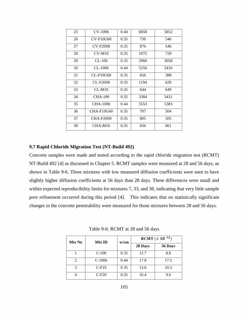
105

25 CV-100h 0.44 6858 5852

26 CV-F10G60 0.35 750 546

27 CV-F20S8 0.35 876 546

28 CV-M10 0.35 1075 729

29 CL-100 0.35 2960 3058

30 CL-100h 0.44 5250 5410

31 CL-F10G60 0.35 656 388

32 CL-F20S8 0.35 1194 629

33 CL-M10 0.35 644 649

34 CHA-100 0.35 3384 3431

35 CHA-100h 0.44 5553 5383

36 CHA-F10G60 0.35 707 504

37 CHA-F20S8 0.35 805 505

38 CHA-M10 0.35 656 661

9.7 Rapid Chloride Migration Test (NT-Build 492)

Concrete samples were made and tested according to the rapid chloride migration test (RCMT)

NT-Build 492 [4] as discussed in Chapter 5. RCMT samples were measured at 28 and 56 days, as

shown in Table 9-6. Three mixtures with low measured diffusion coefficients were seen to have

slightly higher diffusion coefficients at 56 days than 28 days. These differences were small and

within expected reproducibility limits for mixtures 7, 33, and 38, indicating that very little sample

pore refinement occurred during this period [4]. This indicates that no statistically significant

changes in the concrete penetrability were measured for those mixtures between 28 and 56 days.

Table 9-6: RCMT at 28 and 56 days

Mix No Mix ID w/cm RCMT (× 𝟏𝟎−𝟏𝟐)

28 Days 56 Days

1 C-100 0.35 12.7 8.8

2 C-100h 0.44 17.8 17.5

3 C-F10 0.35 13.6 10.3

4 C-F20 0.35 16.4 9.0

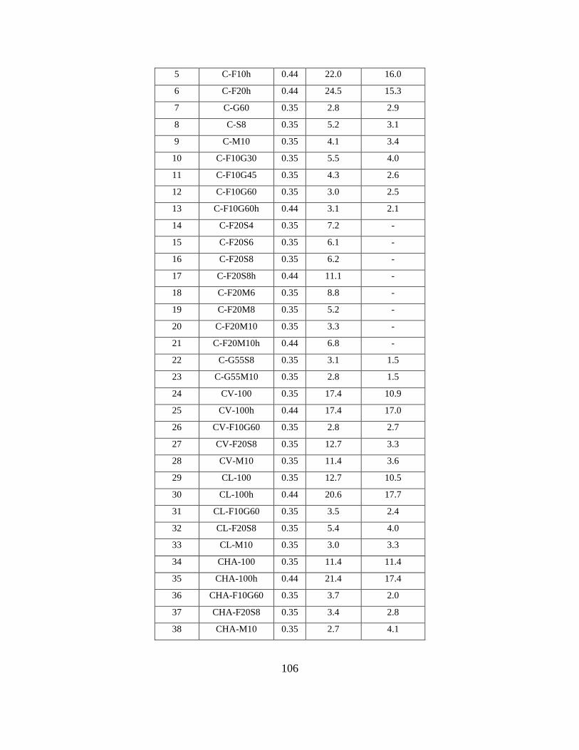
106

5 C-F10h 0.44 22.0 16.0

6 C-F20h 0.44 24.5 15.3

7 C-G60 0.35 2.8 2.9

8 C-S8 0.35 5.2 3.1

9 C-M10 0.35 4.1 3.4

10 C-F10G30 0.35 5.5 4.0

11 C-F10G45 0.35 4.3 2.6

12 C-F10G60 0.35 3.0 2.5

13 C-F10G60h 0.44 3.1 2.1

14 C-F20S4 0.35 7.2 -

15 C-F20S6 0.35 6.1 -

16 C-F20S8 0.35 6.2 -

17 C-F20S8h 0.44 11.1 -

18 C-F20M6 0.35 8.8 -

19 C-F20M8 0.35 5.2 -

20 C-F20M10 0.35 3.3 -

21 C-F20M10h 0.44 6.8 -

22 C-G55S8 0.35 3.1 1.5

23 C-G55M10 0.35 2.8 1.5

24 CV-100 0.35 17.4 10.9

25 CV-100h 0.44 17.4 17.0

26 CV-F10G60 0.35 2.8 2.7

27 CV-F20S8 0.35 12.7 3.3

28 CV-M10 0.35 11.4 3.6

29 CL-100 0.35 12.7 10.5

30 CL-100h 0.44 20.6 17.7

31 CL-F10G60 0.35 3.5 2.4

32 CL-F20S8 0.35 5.4 4.0

33 CL-M10 0.35 3.0 3.3

34 CHA-100 0.35 11.4 11.4

35 CHA-100h 0.44 21.4 17.4

36 CHA-F10G60 0.35 3.7 2.0

37 CHA-F20S8 0.35 3.4 2.8

38 CHA-M10 0.35 2.7 4.1

107

9.8 Bulk (ASTM C1760) and Surface resistivity test (AASHTO T 358)

Samples for bulk and surface resistivity were made and tested as described in Chapter 5. Two

curing environments were used. The first group of samples were cured after demolding in the

moist curing room and the second group were immersed, after demolding, in simulated pore

solution (SPS) in sealed buckets to determine the effects of leaching on resistivity measurements.

The sealed buckets containing the simulated pore solution were kept in the moist curing room to

ensure that they were cured at the same temperature as those cured in the moist curing room. Bulk

and surface resistivity measurements were made at 28, 56, and 91 days after concrete mixing.

Table 9-7 shows the surface and bulk resistivity measurement for curing in SPS. Table 9-8 shows

the surface and bulk resistivity measurements for moist room curing. Bulk resistivity

measurements for mixtures 13, 25, 26, 29, 33, 34, and 36 cured in SPS, and for mixture 1 cured in

the moist curing room, showed slight decreases with age that were well within the 12.34%

acceptable range of results for properly conducted tests by a single operator, indicating no

statistically significant difference in results [105]. Mixture 38 cured in SPS and mixture 24 cured

in the moist room indicated a decrease in bulk resistivity between 28 and 56 days that was just

outside the bounds of acceptable range of results for a single operator, but within the range of

acceptable results for multiple operators.

Table 9-7: Surface and bulk resistivity measurements for SPS curing

Mix No Mix ID w/cm

Surface resistivity (KΩ-cm) Bulk resistivity (KΩ-cm)

28 Days 56 Days 91 Days 28 Days 56 Days 91 Days

1 C-100 0.35 8.98 9.63 10.59 5.11 5.56 6.83

2 C-100h 0.44 5.56 5.85 6.12 2.92 3.48 3.53

3 C-F10 0.35 7.79 9.25 11.13 4.02 5.56 7.35

4 C-F20 0.35 8.21 12.10 14.20 4.26 7.15 10.17

5 C-F10h 0.44 4.57 5.63 6.71 2.86 3.63 4.51

6 C-F20h 0.44 4.65 6.62 9.50 3.01 4.80 7.78

7 C-G60 0.35 16.92 16.34 16.28 11.35 17.24 18.04

8 C-S8 0.35 15.31 19.51 17.67 11.44 17.20 18.91

9 C-M10 0.35 20.03 20.01 20.39 13.79 15.68 18.75

10 C-F10G30 0.35 10.00 11.77 11.33 7.27 11.25 13.63

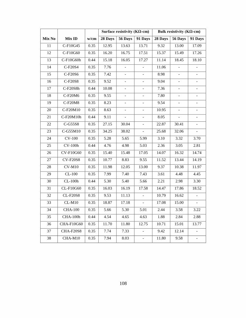
108

Mix No Mix ID w/cm



11 C-F10G45 0.35 12.95 13.63 13.71 9.32 13.00 17.09

12 C-F10G60 0.35 16.20 16.75 17.51 15.37 15.49 17.26

13 C-F10G60h 0.44 15.18 16.05 17.27 11.14 18.45 18.10

14 C-F20S4 0.35 7.76 - - 11.06 - -

15 C-F20S6 0.35 7.42 - - 8.98 - -

16 C-F20S8 0.35 9.52 - - 9.04 - -

17 C-F20S8h 0.44 10.08 - - 7.36 - -

18 C-F20M6 0.35 9.55 - - 7.80 - -

19 C-F20M8 0.35 8.23 - - 9.54 - -

20 C-F20M10 0.35 8.63 - - 10.95 - -

21 C-F20M10h 0.44 9.11 - - 8.05 - -

22 C-G55S8 0.35 27.15 30.04 - 22.87 30.41 -

23 C-G55M10 0.35 34.25 38.02 - 25.68 32.06 -

24 CV-100 0.35 5.28 5.65 5.99 3.10 3.32 3.70

25 CV-100h 0.44 4.76 4.98 5.03 2.36 3.05 2.81

26 CV-F10G60 0.35 15.40 15.48 17.05 14.07 16.32 14.74

27 CV-F20S8 0.35 10.77 8.83 9.55 11.52 13.44 14.19

28 CV-M10 0.35 11.98 12.05 13.00 9.37 10.38 11.97

29 CL-100 0.35 7.99 7.40 7.43 3.61 4.48 4.45

30 CL-100h 0.44 5.30 5.40 5.66 2.21 2.98 3.30

31 CL-F10G60 0.35 16.03 16.19 17.58 14.47 17.86 18.52

32 CL-F20S8 0.35 9.53 11.13 - 10.79 16.62 -

33 CL-M10 0.35 18.87 17.18 - 17.08 15.00 -

34 CHA-100 0.35 5.66 5.30 5.01 2.44 3.58 3.22

35 CHA-100h 0.44 4.54 4.65 4.63 1.88 2.84 2.88

36 CHA-F10G60 0.35 11.70 11.80 12.75 10.71 15.01 13.77

37 CHA-F20S8 0.35 7.74 7.33 - 9.42 12.14 -

38 CHA-M10 0.35 7.94 8.03 - 11.80 9.58 -

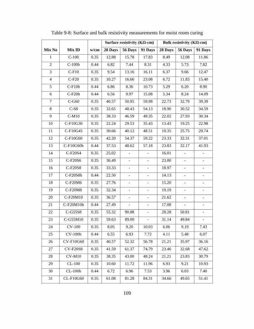
109

Table 9-8: Surface and bulk resistivity measurements for moist room curing

Mix No Mix ID w/cm



1 C-100 0.35 12.88 15.78 17.83 8.49 12.08 11.86

2 C-100h 0.44 6.82 7.44 8.31 4.33 5.73 7.82

3 C-F10 0.35 9.54 13.16 16.11 6.37 9.66 12.47

4 C-F20 0.35 10.27 16.66 23.08 6.72 11.83 15.40

5 C-F10h 0.44 6.86 8.36 10.73 5.29 6.20 8.90

6 C-F20h 0.44 6.56 9.97 15.08 5.34 8.24 14.09

7 C-G60 0.35 40.57 50.95 59.98 22.73 32.79 39.39

8 C-S8 0.35 32.65 48.43 54.13 18.90 30.52 34.59

9 C-M10 0.35 38.33 46.59 49.35 22.02 27.93 30.34

10 C-F10G30 0.35 22.24 29.53 35.43 13.43 19.25 22.98

11 C-F10G45 0.35 30.66 40.12 48.51 19.35 25.75 29.74

12 C-F10G60 0.35 42.20 54.37 59.22 23.33 32.31 37.01

13 C-F10G60h 0.44 37.53 48.62 57.18 23.83 32.17 41.93

14 C-F20S4 0.35 25.02 - - 16.01 - -

15 C-F20S6 0.35 36.49 - - 23.00 - -

16 C-F20S8 0.35 33.33 - - 18.97 - -

17 C-F20S8h 0.44 22.50 - - 14.13 - -

18 C-F20M6 0.35 27.76 - - 15.20 - -

19 C-F20M8 0.35 32.34 - - 19.19 - -

20 C-F20M10 0.35 36.57 - - 21.62 - -

21 C-F20M10h 0.44 27.49 - - 17.08 - -

22 C-G55S8 0.35 55.32 90.88 - 28.28 50.81 -

23 C-G55M10 0.35 59.63 89.00 - 31.14 49.84 -

24 CV-100 0.35 8.05 9.20 10.03 6.06 9.19 7.43

25 CV-100h 0.44 6.55 6.93 7.72 4.11 5.48 6.07

26 CV-F10G60 0.35 40.57 52.32 56.78 21.21 35.97 36.16

27 CV-F20S8 0.35 41.59 61.37 74.79 23.46 32.68 47.62

28 CV-M10 0.35 38.35 43.00 48.24 21.21 23.83 30.79

29 CL-100 0.35 10.60 11.72 11.96 6.93 9.21 10.93

30 CL-100h 0.44 6.72 6.96 7.53 3.96 6.03 7.40

31 CL-F10G60 0.35 61.08 81.28 84.31 34.66 49.65 51.41

110

Mix No Mix ID w/cm



32 CL-F20S8 0.35 29.73 47.84 - 19.35 31.90 -

33 CL-M10 0.35 45.02 48.21 - 25.09 28.71 -

34 CHA-100 0.35 8.60 10.09 10.67 5.41 7.71 10.41

35 CHA-100h 0.44 6.04 6.53 7.25 3.35 4.99 6.60

36 CHA-F10G60 0.35 38.37 49.33 53.81 24.64 32.83 37.29

37 CHA-F20S8 0.35 41.75 57.66 - 24.14 36.73 -

38 CHA-M10 0.35 45.31 45.77 - 24.29 26.48 -

9.9 Discussion

Some trends were found in the preliminary results between material composition and properties

of concrete that are discussed in the following sections.

9.9.1 Effect of Slag Cement

In this section, mixes containing cement I/II with 10 % fly ash, a water-to-cementitious ratio

(w/cm) of 0.35, and slag replacements of 0, 30, 45, and 60% are compared. The slag dosage was

found to have a clear effect on concrete penetrability properties. Figure 9-5 shows that as the slag

replacement increased, the absorption rate decreased. Figure 9-6 shows an inverse relation between

coulombs passed in the rapid chloride permeability test and the slag percentage; as the replacement

increased, the charge passed decreased. Figure 9-7 shows that slag cement had a similar effect on

RCMT results as RCPT.

111

Figure 9-5: Secondary absorption rate (ASTM C1585) vs Slag replacement at 28 days. Samples

contained Type I/II cement and 10% fly ash, with a w/cm of 0.35.

Figure 9-6: Rapid chloride permeability (ASTM C1202) vs slag replacement at 28 days.

Samples contained Type I/II cement and 10% fly ash, with a w/cm of 0.35.

0.E+00

1.E-04

2.E-04

3.E-04

4.E-04

5.E-04

6.E-04

7.E-04

8.E-04

9.E-04

0 10 20 30 40 50 60Sec

on

da

ry a

bso

rpti

on

ra

te (

mm

/s^

0.5

)

Slag (%)

0

500

1000

1500

2000

2500

3000

3500

4000

0 10 20 30 40 50 60

RC

PT

(C

ou

lom

bs)

Slag (%)

112

Figure 9-7: Rapid chloride migration (NT Build 492) vs slag replacement at 28 days. Samples


Figure 9-8 shows the surface resistivity vs slag replacement at 28, 56, and 91 days of moist curing;

as the replacement increased, the surface resistivity increased. Figure 9-9 shows the surface

resistivity vs slag replacement for SPS; accordingly, as slag replacement increased, the surface

resistivity increased, although at much lower values.

Figure 9-8: Surface resistivity (AASHTO T 358) vs slag replacement at different ages (Moist

room). Samples contained Type I/II cement and 10% fly ash, with a w/cm of 0.35.

0

2

4

6

8

10

12

14

16

0 10 20 30 40 50 60

RC

MT

(m

^2/s

) *10

-12

Slag (%)

0

10

20

30

40

50

60

70

0 10 20 30 40 50 60

Su

rface

res

isti

vit

y (

KΩ

-cm

)

Slag (%)

28-days

56-days

91-days

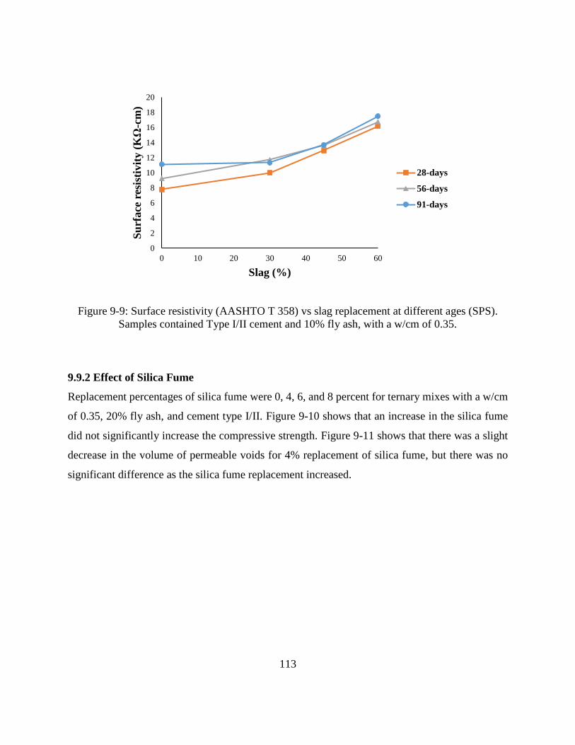
113

Figure 9-9: Surface resistivity (AASHTO T 358) vs slag replacement at different ages (SPS).


9.9.2 Effect of Silica Fume

Replacement percentages of silica fume were 0, 4, 6, and 8 percent for ternary mixes with a w/cm

of 0.35, 20% fly ash, and cement type I/II. Figure 9-10 shows that an increase in the silica fume

did not significantly increase the compressive strength. Figure 9-11 shows that there was a slight

decrease in the volume of permeable voids for 4% replacement of silica fume, but there was no

significant difference as the silica fume replacement increased.

0

2

4

6

8

10

12

14

16

18

20

0 10 20 30 40 50 60

Su

rface

res

isti

vit

y (

KΩ

-cm

)

Slag (%)

28-days

56-days

91-days

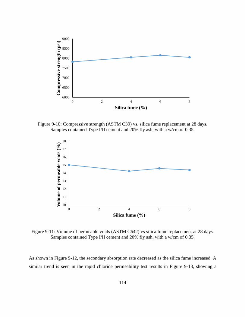
114

Figure 9-10: Compressive strength (ASTM C39) vs. silica fume replacement at 28 days.


Figure 9-11: Volume of permeable voids (ASTM C642) vs silica fume replacement at 28 days.


As shown in Figure 9-12, the secondary absorption rate decreased as the silica fume increased. A

similar trend is seen in the rapid chloride permeability test results in Figure 9-13, showing a

6000

6500

7000

7500

8000

8500

9000

0 2 4 6 8

Com

pre

ssiv

e st

ren

gth

(p

si)

Silica fume (%)

10

11

12

13

14

15

16

17

18

0 2 4 6 8

Volu

me

of

per

mea

ble

void

s (%

)

Silica fume (%)

115

decrease in charge passed of more than 50% for the 4% silica fume addition. Likewise, a decrease

was seen in the rapid chloride migration test results, as shown in Figure 9-14.

Figure 9-12: Secondary absorption rate (ASTM C1585) vs silica fume replacement at 28 days.


Figure 9-13: Rapid chloride permeability (ASTM C1202) vs. silica fume replacement at 28 days.


0.E+00

1.E-04

2.E-04

3.E-04

4.E-04

5.E-04

6.E-04

7.E-04

8.E-04

0 2 4 6 8

Sec

on

da

ry a

bso

rpti

on

ra

te

(mm

/s^

0.5

)

Silica fume (%)

0

500

1000

1500

2000

2500

3000

3500

4000

0 2 4 6 8

RC

PT

(C

ou

lom

bs)

Silica fume (%)

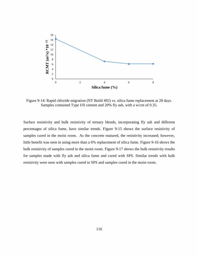
116

Figure 9-14: Rapid chloride migration (NT Build 492) vs. silica fume replacement at 28 days.


Surface resistivity and bulk resistivity of ternary blends, incorporating fly ash and different

percentages of silica fume, have similar trends. Figure 9-15 shows the surface resistivity of

samples cured in the moist room. As the concrete matured, the resistivity increased; however,

little benefit was seen in using more than a 6% replacement of silica fume. Figure 9-16 shows the

bulk resistivity of samples cured in the moist room. Figure 9-17 shows the bulk resistivity results

for samples made with fly ash and silica fume and cured with SPS. Similar trends with bulk

resistivity were seen with samples cured in SPS and samples cured in the moist room.

0

2

4

6

8

10

12

14

16

18

0 2 4 6 8

RC

MT

(m

2/s

) *10 -1

2

Silica fume (%)

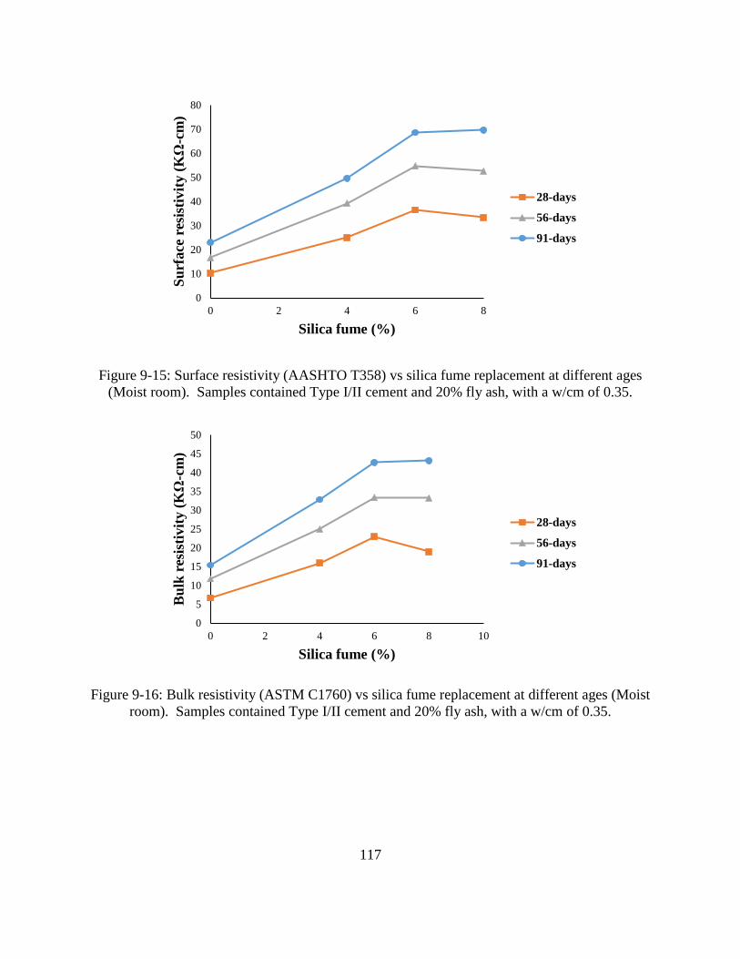
117

Figure 9-15: Surface resistivity (AASHTO T358) vs silica fume replacement at different ages

(Moist room). Samples contained Type I/II cement and 20% fly ash, with a w/cm of 0.35.

Figure 9-16: Bulk resistivity (ASTM C1760) vs silica fume replacement at different ages (Moist


0

10

20

30

40

50

60

70

80

0 2 4 6 8

Su

rface

res

isti

vit

y (

KΩ

-cm

)

Silica fume (%)

28-days

56-days

91-days

0

5

10

15

20

25

30

35

40

45

50

0 2 4 6 8 10

Bu

lk r

esis

tivit

y (

KΩ

-cm

)

Silica fume (%)

28-days

56-days

91-days

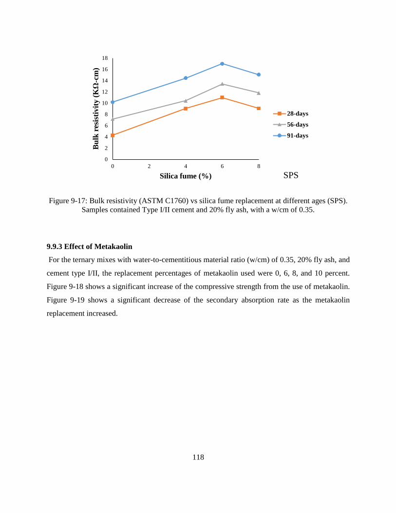
118

Figure 9-17: Bulk resistivity (ASTM C1760) vs silica fume replacement at different ages (SPS).


9.9.3 Effect of Metakaolin

For the ternary mixes with water-to-cementitious material ratio (w/cm) of 0.35, 20% fly ash, and

cement type I/II, the replacement percentages of metakaolin used were 0, 6, 8, and 10 percent.

Figure 9-18 shows a significant increase of the compressive strength from the use of metakaolin.

Figure 9-19 shows a significant decrease of the secondary absorption rate as the metakaolin

replacement increased.

0

2

4

6

8

10

12

14

16

18

0 2 4 6 8

Bu

lk r

esis

tivit

y (

KΩ

-cm

)

Silica fume (%) SPS

28-days

56-days

91-days

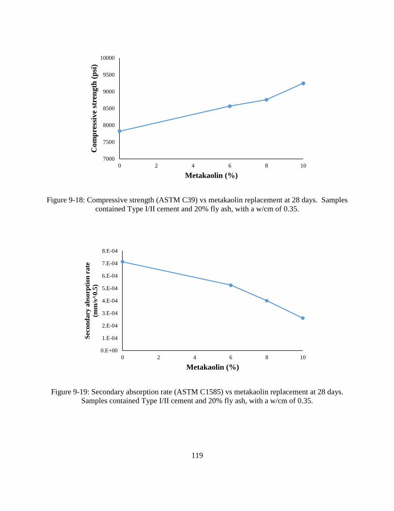
119

Figure 9-18: Compressive strength (ASTM C39) vs metakaolin replacement at 28 days. Samples


Figure 9-19: Secondary absorption rate (ASTM C1585) vs metakaolin replacement at 28 days.


7000

7500

8000

8500

9000

9500

10000

0 2 4 6 8 10

Com

pre

ssiv

e st

ren

gth

(p

si)

Metakaolin (%)

0.E+00

1.E-04

2.E-04

3.E-04

4.E-04

5.E-04

6.E-04

7.E-04

8.E-04

0 2 4 6 8 10

Sec

on

dary

ab

sorp

tion

rate

(mm

/s^

0.5

)

Metakaolin (%)

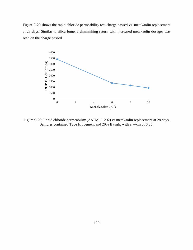
120

Figure 9-20 shows the rapid chloride permeability test charge passed vs. metakaolin replacement

at 28 days. Similar to silica fume, a diminishing return with increased metakaolin dosages was

seen on the charge passed.

Figure 9-20: Rapid chloride permeability (ASTM C1202) vs metakaolin replacement at 28 days.


0

500

1000

1500

2000

2500

3000

3500

4000

0 2 4 6 8 10

RC

PT

(C

ou

lom

bs)

Metakaolin (%)

121

Metakaolin affected the rapid chloride migration significantly as shown in Figure 9-21; using 10%

metakaolin as the replacement dropped the migration rate up to 80%.

Figure 9-21: Rapid chloride migration (NT Build 492) vs metakaolin replacement at 28 days.


Figure 9-22 shows the surface resistivity increased significantly with metakaolin replacement at

28 days, 56 days, and 91 days for samples cured in the moist room; however, SPS-cured samples

showed insignificant changes (Figure 9-23) with metakaolin replacement, possibly because the

SPS concentration was significantly different than expected. Figure 9-24 shows the bulk resistivity

vs metakaolin replacement for the moist room curing at 28 days, 56 days, and 91 days.

0

2

4

6

8

10

12

14

16

18

0 2 4 6 8 10

RC

MT

(m

2/s

) *10

-12

Metakaolin (%)

122


(moist room). Samples contained Type I/II cement and 20% fly ash, with a w/cm of 0.35.


(SPS). Samples contained Type I/II cement and 20% fly ash, with a w/cm of 0.35.

0

10

20

30

40

50

60

0 2 4 6 8 10

Su

rface

res

isti

vit

y (

KΩ

-cm

)

Metakaolin (%)

28-days

56-days

91-days

0

2

4

6

8

10

12

14

16

0 2 4 6 8 10

Su

rface

res

isti

vit

y (

KΩ

-cm

)

Metakaolin (%)

28-days

56-days

91-days

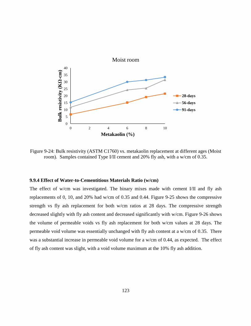
123

Figure 9-24: Bulk resistivity (ASTM C1760) vs. metakaolin replacement at different ages (Moist


9.9.4 Effect of Water-to-Cementitious Materials Ratio (w/cm)

The effect of w/cm was investigated. The binary mixes made with cement I/II and fly ash

replacements of 0, 10, and 20% had w/cm of 0.35 and 0.44. Figure 9-25 shows the compressive

strength vs fly ash replacement for both w/cm ratios at 28 days. The compressive strength

decreased slightly with fly ash content and decreased significantly with w/cm. Figure 9-26 shows

the volume of permeable voids vs fly ash replacement for both w/cm values at 28 days. The

permeable void volume was essentially unchanged with fly ash content at a w/cm of 0.35. There

was a substantial increase in permeable void volume for a w/cm of 0.44, as expected. The effect

of fly ash content was slight, with a void volume maximum at the 10% fly ash addition.

0

5

10

15

20

25

30

35

40

0 2 4 6 8 10

Bu

lk r

esis

tivit

y (

KΩ

-cm

)

Metakaolin (%)

Moist room

28-days

56-days

91-days

124

Figure 9-25: Compressive strength (ASTM C39) vs. fly ash replacement and w/cm ratio at 28

days. Samples contained Type I/II cement.

Figure 9-26: Volume of permeable voids (ASTM C642) vs. fly ash and w/cm ratio replacement

at 28 days. Samples contained Type I/II cement.

Figure 9-27 shows the secondary absorption rate vs. fly ash replacement for w/cm of 0.35 and

0.44. The higher w/cm ratio had a higher absorption rate, as expected, due to the higher permeable

void volume, and as the fly ash replacement increased, the absorption rate decreased.

0

1000

2000

3000

4000

5000

6000

7000

8000

9000

0 5 10 15 20

Com

pre

ssiv

e st

ren

gth

(p

si)

Fly ash (%)

w/c=0.35

w/c=0.44

10

11

12

13

14

15

16

17

18

19

20

0 5 10 15 20

Volu

me

of

per

mea

ble

void

s (%

)

Fly ash (%)

w/c=0.35

w/c=0.44

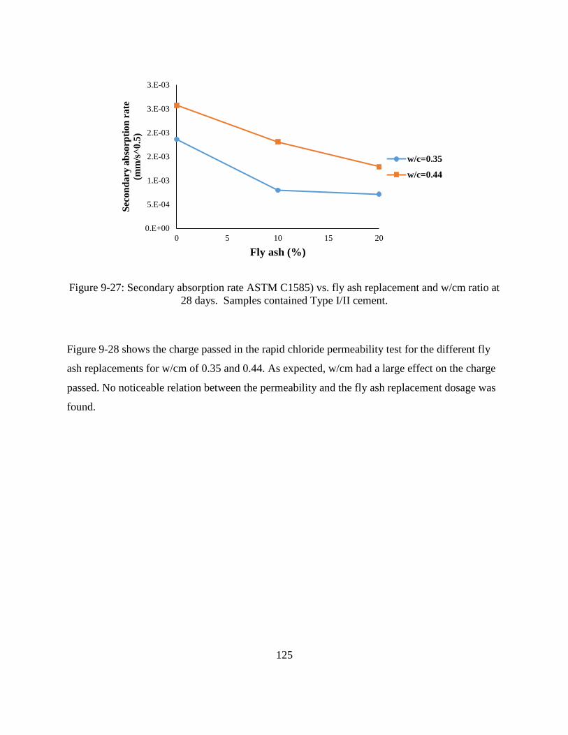
125

Figure 9-27: Secondary absorption rate ASTM C1585) vs. fly ash replacement and w/cm ratio at

28 days. Samples contained Type I/II cement.

Figure 9-28 shows the charge passed in the rapid chloride permeability test for the different fly

ash replacements for w/cm of 0.35 and 0.44. As expected, w/cm had a large effect on the charge

passed. No noticeable relation between the permeability and the fly ash replacement dosage was

found.

0.E+00

5.E-04

1.E-03

2.E-03

2.E-03

3.E-03

3.E-03

0 5 10 15 20

Sec

on

da

ry a

bso

rpti

on

ra

te

(mm

/s^

0.5

)

Fly ash (%)

w/c=0.35

w/c=0.44

126

Figure 9-28: Rapid chloride permeability (ASTM C1202) vs. fly ash and w/cm ratio replacement

at 28 days. Samples contained Type I/II cement.

Figure 9-29 shows the rapid chloride migration vs fly ash replacement for w/cm of 0.44 and 0.35

at 28 days; as the fly ash increased, the diffusion from migration increased, and as the w/cm

increased, the migration results increased.

Figure 9-29: Rapid chloride migration (NT Build 492) vs. fly ash replacement and w/cm ratio at

28 days. Samples contained Type I/II cement.

0

1000

2000

3000

4000

5000

6000

7000

0 5 10 15 20

RC

PT

(C

ou

lom

bs)

Fly ash (%)

w/c=0.35

w/c=0.44

0

5

10

15

20

25

30

0 5 10 15 20

RC

MT

(m

^2/s

) *10

-12

Fly ash (%)

w/c=0.35

w/c=0.44

127

9.10 Comparison between Test Methods

Some trends were found between test methods and concrete properties in the preliminary data that

merit examination. It is known that strength is a function of the gel porosity [106]. The relationship

between the compressive strength and volume of permeable voids at 28 days is shown in Figure

9-30. This relationship demonstrates that while the volume of permeable voids is not a direct

measure of the paste gel porosity, they are related. SCM use at 28 days increased the variance

between the compressive strength and volume of permeable voids, most likely because the fly ash

at 28 days was not well reacted. The compressive strength was shown to have a weak inverse

relation with absorption rate as shown in Figure 9-31. Water absorption is greatly affected by both

the pore size distribution and volume, whereas compressive strength is more related to the pore

volume [107].

Figure 9-30: Compressive strength vs. volume of permeable voids at 28 days

4000

5000

6000

7000

8000

9000

10000

12 14 16 18 20

Co

mp

ress

ive

Str

eng

th (

psi

)

Volume of Permeable voids (%)

No SCM w/cm:Low

No SCM w/cm:High

Binary w/cm:Low

Binary w/cm:High

Ternary w/cm:Low

Ternary w/cm:High

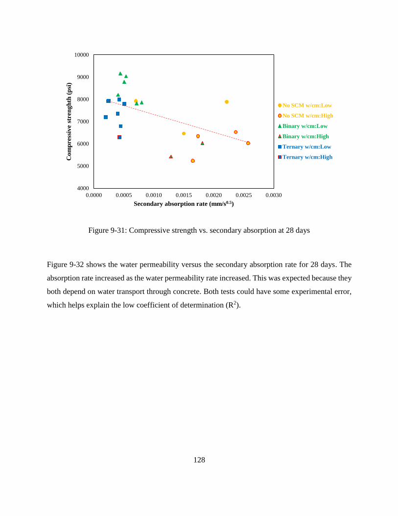
128

Figure 9-31: Compressive strength vs. secondary absorption at 28 days

Figure 9-32 shows the water permeability versus the secondary absorption rate for 28 days. The

absorption rate increased as the water permeability rate increased. This was expected because they

both depend on water transport through concrete. Both tests could have some experimental error,

which helps explain the low coefficient of determination (R2).

4000

5000

6000

7000

8000

9000

10000

0.0000 0.0005 0.0010 0.0015 0.0020 0.0025 0.0030

Co

mp

ress

ive

stre

ng

hth

(p

si)

Secondary absorption rate (mm/s0.5)

No SCM w/cm:Low

No SCM w/cm:High

Binary w/cm:Low

Binary w/cm:High

Ternary w/cm:Low

Ternary w/cm:High

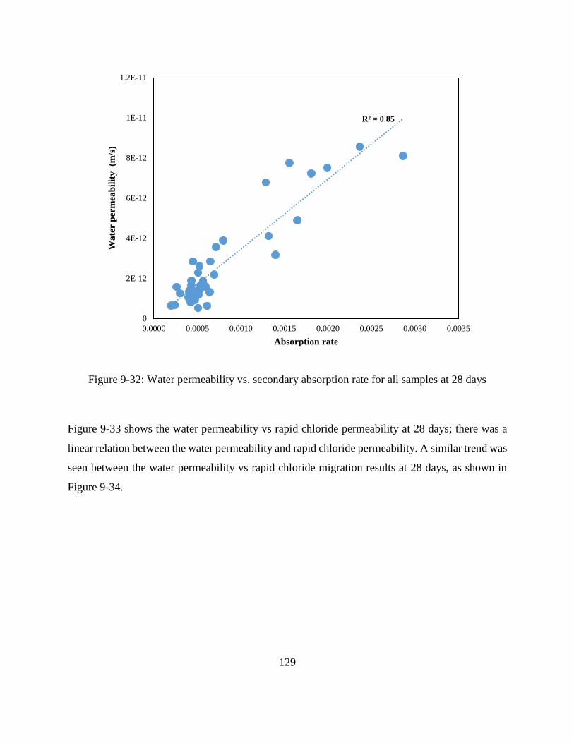
129

Figure 9-32: Water permeability vs. secondary absorption rate for all samples at 28 days

Figure 9-33 shows the water permeability vs rapid chloride permeability at 28 days; there was a

linear relation between the water permeability and rapid chloride permeability. A similar trend was

seen between the water permeability vs rapid chloride migration results at 28 days, as shown in

Figure 9-34.

R² = 0.85

0

2E-12

4E-12

6E-12

8E-12

1E-11

1.2E-11

0.0000 0.0005 0.0010 0.0015 0.0020 0.0025 0.0030 0.0035

Wa

ter p

erm

eab

ilit

y

(m/s

)

Absorption rate

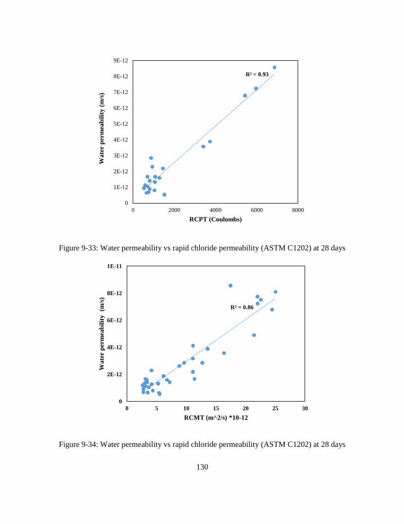
130

Figure 9-33: Water permeability vs rapid chloride permeability (ASTM C1202) at 28 days

Figure 9-34: Water permeability vs rapid chloride permeability (ASTM C1202) at 28 days

R² = 0.93

0

1E-12

2E-12

3E-12

4E-12

5E-12

6E-12

7E-12

8E-12

9E-12

0 2000 4000 6000 8000

Wa

ter p

erm

eab

ilit

y (

m/s

)

RCPT (Coulombs)

R² = 0.86

0

2E-12

4E-12

6E-12

8E-12

1E-11

0 5 10 15 20 25 30

Wa

ter p

erm

eab

ilit

y

(m/s

)

RCMT (m^2/s) *10-12

131

A linear relationship between the initial and secondary absorption rate is shown in Figure 9-35.

The ternary blend mixtures had on average the lowest water absorption rate, likely due to pore

refinement increasing the tortuosity of the interconnected capillary network.

Figure 9-35: Initial and secondary absorption rate for each mix group

A comparison of the different concrete electrical test methods showed the strong relationship

between each test. Figure 9-36 shows the relation between rapid chloride migration and rapid

chloride permeability test results at 28 days. The RCMT is not a pure electrical test. It measures

diffusion of chloride ions in concrete exposed to an electrical potential. The surface resistivity

was compared to the RCPT results for samples cured in the moist curing room and SPS in Figure

9-37. The coefficient of determination (R2) for the surface resistivity samples cured in the moist

curing room was much higher than for the SPS-cured samples kept in the moist curing room. This

0.000

0.001

0.002

0.003

0.004

0.005

0.006

0.000 0.001 0.002 0.003

Init

ial

ab

sorp

tio

n r

ate

(m

m/s

0.5

)


No SCM w/cm:Low

No SCM w/cm:High

Binary w/cm:Low

Binary w/cm:High

Ternary w/cm:Low

Ternary w/cm:High

132

could be explained by considering that the RCPT samples exposed to the moist air in the moist

room likely leached in a manner similar to the surface resistivity samples cured in the moist room

[108]. Thus, the microstructures (porosity and tortuosity) and, consequently, the fluid transport of

the leached SR and RCPT samples could be much more alike than the unleached (SPS) and leached

SR samples.

Figure 9-36: RCMT vs. RCPT at 28 days

0

1000

2000

3000

4000

5000

6000

7000

0 5 10 15 20 25 30

RC

PT

(C

ou

lom

bs)

RCMT (10-12 m2/s)

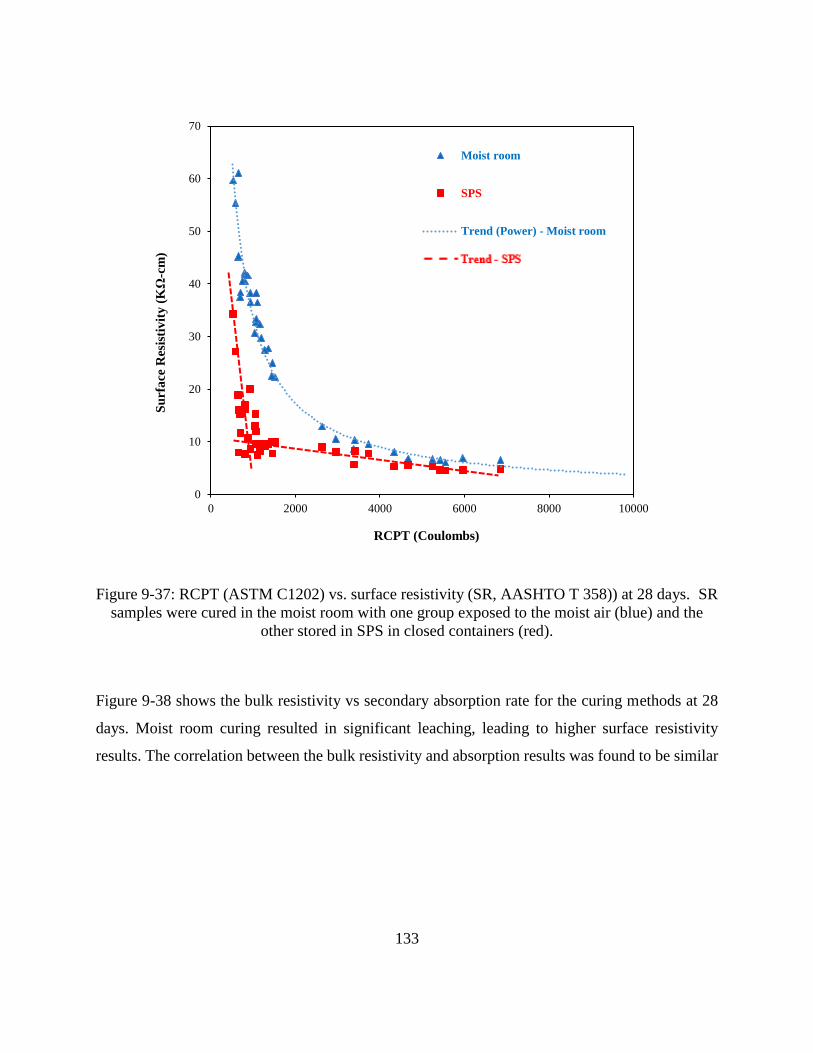
133

Figure 9-37: RCPT (ASTM C1202) vs. surface resistivity (SR, AASHTO T 358)) at 28 days. SR

samples were cured in the moist room with one group exposed to the moist air (blue) and the

other stored in SPS in closed containers (red).

Figure 9-38 shows the bulk resistivity vs secondary absorption rate for the curing methods at 28

days. Moist room curing resulted in significant leaching, leading to higher surface resistivity

results. The correlation between the bulk resistivity and absorption results was found to be similar

0

10

20

30

40

50

60

70

0 2000 4000 6000 8000 10000

Su

rfa

ce R

esis

tiv

ity

(K

Ω-c

m)

RCPT (Coulombs)

Moist room

SPS

Trend (Power) - Moist room

134

for both methods of curing. This is because the absorption results, unlike the RCPT results, are not

dependent on the concrete pore solution conductivity.

Figure 9-38: Bulk resistivity vs. secondary absorption rate at 28 days

Comparison of the bulk and surface resistivity results in Figure 9-39 helps illustrate the problem

with leaching in concrete samples in the moist curing room. Calcium hydroxide and alkalis will

leach from the outside surface, giving lower pore solution concentrations at the surface than

interior. This will result in differences between the surface and bulk resistivity results because

leaching will affect the surface resistivity results more than bulk resistivity measurements [109].

R² = 0.82

R² = 0.83

0

5

10

15

20

25

30

35

40

0.000 0.001 0.002 0.003

Bu

lk r

esis

tivit

y (

KΩ

-cm

)


Moist room

SPS

Trend (Power) - Moist room

Trend (Power) - SPS

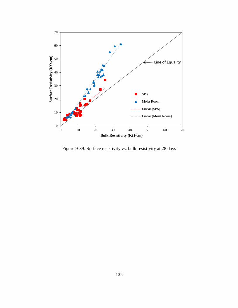
135

Figure 9-39: Surface resistivity vs. bulk resistivity at 28 days

0

10

20

30

40

50

60

70

0 10 20 30 40 50 60 70

Su

rfa

ce R

esis

tiv

ity

(K

Ω-c

m)

Bulk Resistivity (KΩ-cm)

SPS

Moist Room

Linear (SPS)

Linear (Moist Room)

Line of Equality

136

CHAPTER 10. CONCLUSIONS AND RECOMMENDATIONS

Concrete mixture performance for marine environments has been measured using surface

resistivity measurements (AASHTO T358). Concern over the ability of this test to reliably indicate

long-term durability for the wide variety of cementitious material combinations in use led to

development of a testing program to quantify the correlation of the surface resistivity test to other

concrete water and ionic transport tests. As part of this phase I study, samples were fabricated to

measure the concrete surface resistivity (AASHTO T358), bulk resistivity (AASHTO TP119),

rapid chloride permeability (ASTM C1202), rapid chloride migration (NT-Build 492), water

absorption (ASTM C1585), water permeability, and volume of permeable voids (ASTM C642).

Some mixtures were made with #89 aggregates to measure the concrete pore system using mercury

intrusion porosimetry. Samples were made to test at 28, 56, and 365 days. Samples were also made

for bulk diffusion testing (ASTM C1556) after 6 and 12 months of chloride exposure. In addition,

samples were fabricated to measure the concrete expansion after exposure to a 5% sodium sulfate

solution. Preliminary results indicate that the surface resistivity measurements correlate well to the

concrete water absorption, rapid chloride permeability, and rapid chloride migration test results. It

is recommended that the samples tested under this phase I project be tested under a phase II project

to confirm the ability of the surface resistivity test, and to test the feasibility of using the formation

factor to predict mixture water and ionic transport properties.

137

REFERENCES

[1] AASHTO T358-15. Standard Method of Test for Surface Resistivity Indication of Concrete’s

Ability to Resist Chloride Ion Penetration. American Association of State Highway and

Transportation Officials, Washington, D.C. 2015.

[2] AASHTO TP 119-15. Standard Method of Test for Electrical Resistivity of a Concrete Cylinder

Tested in a Uniaxial Resistance Test. American Association of State Highway and Transportation

Officials, Washington, D.C. 2015.

[3] ASTM C1202-12. Standard Test Method for Electrical Indication of Concrete's Ability to

Resist Chloride Ion Penetration. ASTM International, West Conshohocken, PA 23 Feb 2017.

[4] NT Build 492. Concrete, Mortar and Cement-based Repair Materials: Chloride Migration

Coefficient from Non-steady-state Migration Experiments. Nordtest Method 1999.

[5] Smith D. The development of a rapid test for determining the transport properties of concrete.

Portland Cement Association 2006:125.

[6] Spragg R, Bu Y, Snyder K, Bentz D, Weiss J. Electrical testing of cement-based materials:

Role of testing techniques, sample conditioning, and accelerated curing. Publication

FHWA/IN/JTRP-2013/28. Joint Transportation Research Program, Indiana Department of

Transportation and Purdue University, West Lafayette, Indiana, 2013.

[7] Bentz DP. A virtual rapid chloride permeability test. Cement and Concrete Composites

2007;29:723-31.

[8] DeFord HD. Personal Communication. August 30, 2016.

[9] ASTM C1585 − 13. Standard Test Method for Measurement of Rate of Absorption of Water

by Hydraulic Cement Concretes. ASTM International, West Conshohocken, PA 2013.

[10] ASTM C1556-11a. Standard Test Method for Determining the Apparent Chloride Diffusion

Coefficient of Cementitious Mixtures by Bulk Diffusion. ASTM International, West

Conshohocken, PA 2016.

138

[11] Irassar E, Di Maio A, Batic O. Sulfate attack on concrete with mineral admixtures. Cem Concr

Res 1996;26:113-23.

[12] Kurdowski W. Cement and concrete chemistry. Springer Science & Business, 2014.

[13] Bentz D, Garboczi E, Martys N, Snyder K, Guthrie W, Kyritsis K et al. Virtual testing of

concrete transport properties. submitted to ACI Fall 2009 session on Material Science Modeling

as a Solution to Concrete Problems 2009.

[14] Pitroda J, Umrigar DF, Principal B, Anand G. Evaluation of sorptivity and water absorption

of concrete with partial replacement of cement by thermal industry waste (Fly Ash). International

Journal of Engineering and Innovative Technology (IJEIT) Volume 2013;2.

[15] Claisse P. Transport Properties of Concrete. Concrete International 2005;27:43-8.

[16] Rajabipour F, Sant G, Weiss J. Development of electrical conductivity-based sensors for

health monitoring of concrete materials. TRB 86th Annual Meeting Compendium of Papers CD-

ROM 2007.

[17] Luping T, Gulikers J. On the mathematics of time-dependent apparent chloride diffusion

coefficient in concrete. Cem Concr Res 2007;37:589-95.

[18] Dolen TP, Scott GA, von Fay KF, Hamilton B. Effects of Concrete Deterioration on Safety

of Dams. Report No. DSO-03-05, Department of the Interior, Bureau of Reclamation. December

2003.

[19] Drimalas T. Laboratory and field evaluations of external sulfate attack. The University of

Texas at Austin, 2007.

[20] Lampacher B, Blight G. Permeability and sorption properties of mature near-surface concrete.

J Mater Civ Eng 1998;10:21-5.

[21] Andrade C. Calculation of chloride diffusion coefficients in concrete from ionic migration

measurements. Cem Concr Res 1993;23:724-42.

[22] Xiao L, Ren Z, Shi W, Wei X. Experimental study on chloride permeability in concrete by

non-contact electrical resistivity measurement and RCM. Constr Build Mater 2016;123:27-34.

139

[23] Zibara H. Binding of external chlorides by cement pastes. University of Toronto 2001.

[24] Yuan Q, Shi C, De Schutter G, Audenaert K, Deng D. Chloride binding of cement-based

materials subjected to external chloride environment - A review. Construction and Building

Materials 2009;23:1-13.

[25] Richartz W. Die Bindung von Chlorid bei der Zementerhärtung. Zement-Kalk-Gips

1969;22:447-56.

[26] Ben-Yair M. The effect of chlorides on concrete in hot and arid regions. Cem Concr Res

1974;4:405-16.

[27] Glasser F. Role of chemical binding in diffusion and mass transport. 1999:129-54.

[28] Larsen C. Chloride binding in concrete, Effect of surrounding environment and concrete

composition. Dr.ing.Thesis, NTNU, Trondheim 1998;95:337-0.

[29] Tuutti K. Corrosion of steel in concrete. Swedish Cement and Concrete Research Institute,

Stockholms 1982.

[30] Ramachandran VS, Seeley R, Polomark G. Free and combined chloride in hydrating cement

and cement components. Mater Struct 1984;17:285-9.

[31] Luping T, Nilsson L. Chloride binding capacity and binding isotherms of OPC pastes and

mortars. Cem Concr Res 1993;23:247-53.

[32] Arya C, Buenfeld N, Newman J. Factors influencing chloride-binding in concrete. Cem Concr

Res 1990;20:291-300.

[33] Justnes H. A review of chloride binding in cementitious systems. NORDIC CONCRETE

RESEARCH-PUBLICATIONS- 1998;21:48-63.

[34] Beaudoin JJ, Ramachandran VS, Feldman RF. Interaction of chloride and C-S-H. Cem Concr

Res 1990;20:875-83.

[35] Tritthart J. Chloride binding in cement II. The influence of the hydroxide concentration in the

pore solution of hardened cement paste on chloride binding. Cem Concr Res 1989;19:683-91.

140

[36] Suryavanshi A, Scantlebury J, Lyon S. Mechanism of Friedel's salt formation in cements rich

in tri-calcium aluminate. Cem Concr Res 1996;26:717-27.

[37] Suryavanshi A, Swamy RN. Stability of Friedel's salt in carbonated concrete structural

elements. Cem Concr Res 1996;26:729-41.

[38] Chalee W, Jaturapitakkul Ca, Chindaprasirt P. Predicting the chloride penetration of fly ash

concrete in seawater. Mar Struct 2009;22:341-53.

[39] Ahmed MS, Kayali O, Anderson W. Chloride penetration in binary and ternary blended

cement concretes as measured by two different rapid methods. Cement and Concrete Composites

2008;30:576-82.

[40] ASTM C1543-10a. Standard Test Method for Determining the Penetration of Chloride Ion

into Concrete by Ponding. ASTM International, West Conshohocken, PA 2010.

[41] Spiesz P, Brouwers H. Influence of the applied voltage on the Rapid Chloride Migration

(RCM) test. Cem Concr Res 2012;42:1072-82.

[42] Hooton R, Titherington M. Chloride resistance of high-performance concretes subjected to

accelerated curing. Cem Concr Res 2004;34:1561-7.

[43] Dias W. Reduction of concrete sorptivity with age through carbonation. Cem Concr Res

2000;30:1255-61.

[44] Castro J, Bentz D, Weiss J. Effect of sample conditioning on the water absorption of concrete.

Cement and Concrete Composites 2011;33:805-13.

[45] Li W, Pour-Ghaz M, Castro J, Weiss J. Water absorption and critical degree of saturation

relating to freeze-thaw damage in concrete pavement joints. J Mater Civ Eng 2011;24:299-307.

[46] Claisse PA, Elsayad HI, Shaaban IG. Absorption and sorptivity of cover concrete. J Mater

Civ Eng 1997;9:105-10.

[47] BS 1881-5. Testing concrete. Methods of testing hardened concrete for other than strength.

BSI 1970.

141

[48] Soongswang P, Tia M, Bloomquist DG, Meletiou C, Sessions LM. Efficient test setup for

determining the water-permeability of concrete. Transp Res Rec 1988.

[49] Abbas A, Carcasses M, Ollivier J-. Gas permeability of concrete in relation to its degree of

saturation. Mater Struct 1999;32:3-8.

[50] Aldea C, Shah SP, Karr A. Effect of cracking on water and chloride permeability of concrete.

J Mater Civ Eng 1999;11:181-7.

[51] Ludirdja D, Berger RL, Young J. Simple method for measuring water permeability of

concrete. Materials Journal 1989;86:433-9.

[52] Wang K, Jansen DC, Shah SP, Karr AF. Permeability study of cracked concrete. Cem Concr

Res 1997;27:381-93.

[53] Shi H, Xu B, Zhou X. Influence of mineral admixtures on compressive strength, gas

permeability and carbonation of high performance concrete. Constr Build Mater 2009;23:1980-5.

[54] Kollek J. The determination of the permeability of concrete to oxygen by the Cembureau

method—a recommendation. Mater Struct 1989;22:225-30.

[55] Kumar R, Bhattacharjee B. Porosity, pore size distribution and in situ strength of concrete.

Cem Concr Res 2003;33:155-64.

[56] Abell A, Willis K, Lange D. Mercury intrusion porosimetry and image analysis of cement-

based materials. J Colloid Interface Sci 1999;211:39-44.

[57] Giesche H. Mercury porosimetry: a general (practical) overview. Particle & particle systems

characterization 2006;23:9-19.

[58] Cook RA, Hover KC. Mercury porosimetry of hardened cement pastes. Cem Concr Res

1999;29:933-43.

[59] ASTM C642-13. Standard Test Method for Density, Absorption, and Voids in Hardened

Concrete. ASTM International, West Conshohocken, PA 2013.

142

[60] Ramezanianpour A, Jovein HB. Influence of metakaolin as supplementary cementing material

on strength and durability of concretes. Constr Build Mater 2012;30:470-9.

[61] Feldman RF, Chan GW, Brousseau RJ, Tumidajski PJ. Investigation of the rapid chloride

permeability test. Materials Journal 1994;91:246-55.

[62] Shi C. Effect of mixing proportions of concrete on its electrical conductivity and the rapid

chloride permeability test (ASTM C1202 or ASSHTO T277) results. Cem Concr Res 2004;34:537-

45.

[63] Shi C, Stegemann JA, Caldwell RJ. Effect of supplementary cementing materials on the

specific conductivity of pore solution and its implications on the rapid chloride permeability test

(AASHTO T277 and ASTM C1202) results. Materials Journal 1998;95:389-94.

[64] Andersson K, Allard B, Bengtsson M, Magnusson B. Chemical composition of cement pore

solutions. Cem Concr Res 1989;19:327-32.

[65] Snyder K. The relationship between the formation factor and the diffusion coefficient of

porous materials saturated with concentrated electrolytes: theoretical and experimental

considerations. Concrete Science and Engineering 2001;3:216-24.

[66] Spragg R, Qiao C, Barrett T, Weiss J. Assessing a concrete’s resistance to chloride ion ingress

using the formation factor. Elsevier, London, 2016.

[67] Rajabipour F, Weiss J. Electrical conductivity of drying cement paste. Mater Struct

2007;40:1143-60.

[68] McCarter W, Starrs G, Chrisp T. Electrical conductivity, diffusion, and permeability of

Portland cement-based mortars. Cem Concr Res 2000;30:1395-400.

[69] ASTM C618-15. Standard Specification for Coal Fly Ash and Raw or Calcined Natural

Pozzolan for Use in Concrete. ASTM International, West Conshohocken, PA 2015.

[70] Nochaiya T, Wongkeo W, Chaipanich A. Utilization of fly ash with silica fume and properties

of Portland cement–fly ash–silica fume concrete. Fuel 2010;89:768-74.

[71] Bapat JD. Mineral admixtures in cement and concrete. : CRC Press, 2012.

143

[72] Oner A, Akyuz S. An experimental study on optimum usage of GGBS for the compressive

strength of concrete. Cement and Concrete Composites 2007;29:505-14.

[73] Häkkinen T. The influence of slag content on the microstructure, permeability and mechanical

properties of concrete Part 1 Microstructural studies and basic mechanical properties. Cem Concr

Res 1993;23:407-21.

[74] Wiens U, Schiessl P. Chloride binding of cement paste containing fly ash. Proceedings of the

10th ICCC, Goteborg, Sweden 1997:4-10.

[75] S. Muthulingam, B. N. Rao. Chloride binding and time-dependent surface chloride content

models for fly ash concrete. Frontiers of Structural and Civil Engineering 2016;10:112-20.

[76] Sumranwanich T, Tangtermisiriku S. A chloride binding capacity model for cement-fly ash

pastes. 2002:29-30.

[77] Kayali O, Khan M, Ahmed MS. The role of hydrotalcite in chloride binding and corrosion

protection in concretes with ground granulated blast furnace slag. Cement and Concrete

Composites 2012;34:936-45.

[78] Page C, Vennesland Ø. Pore solution composition and chloride binding capacity of silica-

fume cement pastes. Matériaux et Construction 1983;16:19-25.

[79] Coleman N, Page C. Aspects of the pore solution chemistry of hydrated cement pastes

containing metakaolin. Cem Concr Res 1997;27:147-54.

[80] Saikia N, Kato S, Kojima T. Thermogravimetric investigation on the chloride binding

behaviour of MK–lime paste. Thermochimica Acta 2006;444:16-25.

[81] Hussain SE. Corrosion resistance performance of fly ash blended cement concrete. Materials

Journal 1994;91:264-72.

[82] Vuk T, Tinta V, Gabrovšek R, Kaučič V. The effects of limestone addition, clinker type and

fineness on properties of Portland cement. Cem Concr Res 2001;31:135-9.

[83] ASTM C150/C150M-16e1. Standard Specification for Portland Cement. ASTM

International, West Conshohocken, PA 2016.

144

[84] Florida Department of Transportation. STANDARD SPECIFICATIONS FOR ROAD AND

BRIDGE CONSTRUCTION. Jan 2016.

[85] Erdem TK, Kırca Ö. Use of binary and ternary blends in high strength concrete. Constr Build

Mater 2008;22:1477-83.

[86] Khan M, Lynsdale C. Strength, permeability, and carbonation of high-performance concrete.

Cem Concr Res 2002;32:123-31.

[87] ASTM C989/C989M-16. Standard Specification for Slag Cement for Use in Concrete and

Mortars. ASTM International, West Conshohocken, PA 2016.

[88] ASTM C1240-15. Standard Specification for Silica Fume Used in Cementitious Mixtures.

ASTM International, West Conshohocken, PA 2015.

[89] ASTM C33/C33M-16e1. Standard Specification for Concrete Aggregates. ASTM


[90] ASTM C494/C494M-16. Standard Specification for Chemical Admixtures for Concrete.


[91] ASTM C127-15. Standard Test Method for Relative Density (Specific Gravity) and

Absorption of Coarse Aggregate. ASTM International, West Conshohocken, PA 2015.

[92] ASTM C136/C136M-14. Standard Test Method for Sieve Analysis of Fine and Coarse

Aggregates. ASTM International, West Conshohocken, PA 2014.

[93] ASTM C128-15. Standard Test Method for Relative Density (Specific Gravity) and

Absorption of Fine Aggregate. ASTM International, West Conshohocken, PA 2015.

[94] ASTM C192/C192M-16a. Standard Practice for Making and Curing Concrete Test Specimens

in the Laboratory. ASTM International, West Conshohocken, PA 2016.

[95] ASTM C143/C143M-15a. Standard Test Method for Slump of Hydraulic-Cement Concrete.


145

[96] ASTM C138/C138M-09. Standard Test Method for Density (Unit Weight), Yield, and Air

Content (Gravimetric) of Concrete. ASTM International, West Conshohocken, PA 2009.

[97] ASTM C231-09. Standard Test Method for Air Content of Freshly Mixed Concrete by the

Pressure Method. ASTM International, West Conshohocken, PA 2009.

[98] ASTM C1064/C1064M-01. Standard Test Method for Temperature of Freshly Mixed

Portland Cement Concrete. ASTM International, West Conshohocken, PA 2001.

[99] ASTM C42/C42M-16. Standard Test Method for Obtaining and Testing Drilled Cores and

Sawed Beams of Concrete. ASTM International, West Conshohocken, PA 2016.

[100] ASTM C1738/C1738M-14. Standard Practice for High-Shear Mixing of Hydraulic Cement

Pastes. ASTM International, West Conshohocken, PA 2014.

[101] ASTM C490-07. Standard Practice for Use of Apparatus for the Determination of Length

Change of Hardened Cement Paste, Mortar, and Concrete. ASTM International, West

Conshohocken, PA 2007.

[102] ASTM C511-13. Standard Specification for Mixing Rooms, Moist Cabinets, Moist Rooms,

and Water Storage Tanks Used in the Testing of Hydraulic Cements and Concretes. ASTM


[103] ASTM C1012/C1012M-15. Standard Test Method for Length Change of Hydraulic-Cement

Mortars Exposed to a Sulfate Solution. ASTM International, West Conshohocken, PA 2015.

[104] ASTM C39/C39M-18. Standard Test Method for Compressive Strength of Cylindrical

Concrete Specimens. ASTM International, West Conshohocken, PA 2018.

[105] Spragg RP, Castro J, Nantung T, Paredes M, Weiss J. Variability analysis of the bulk

resistivity measured using concrete cylinders. Advances in Civil Engineering Materials 2012;1:1-

17.

[106] Zingg L, Briffaut M, Baroth J, Malecot Y. Influence of cement matrix porosity on the triaxial

behaviour of concrete. Cement and Concrete Research 2016;80:52-9.

146

[107] Iffat S. Relation Between Density and Compressive Strength of Hardened Concrete.

Concrete Research Letters 2015;6:182-9.

[108] Ghosh P, Tran Q. Correlation between bulk and surface resistivity of concrete. International

Journal of Concrete Structures and Materials 2015;9:119-32.

[109] Spragg R, Jones S, Bu Y, Lu Y, Bentz D, Snyder K et al. Leaching of conductive species:

Implications to measurements of electrical resistivity. Cement and Concrete Composites

2017;79:94-105.

final report fdot contract number: bdv-31 … · vi executive summary background the florida...

Documents