Final Report

To Conduct a Pilot Study for How Compensation Earning Data Could Be Collected From Employers on EEOC’s Survey Collection Systems (EEO-1, EEO-4, and EEO-5 Survey Reports) and Develop Burden Cost Estimates for Both EEOC and Respondents for Each of EEOC Surveys (EEO-1, EEO-4, and EEO-5)

Dated: September 2015

Submitted to:

EEOC

Submitted By:

Sage Computing

Authors and Acknowledgment This research was directed by Fidan Kurtulus, Associate Professor of Economics at the University of Massachusetts Amherst and Conrad Miller, Postdoctoral Research Associate in the Industrial Relations Section at Princeton University. Constance F. Citro, Ph.D., director of the Committee on National Statistics at the National Science Foundation provided technical review of the report. The statistical issues in the analysis of pay disparities section was written by Stanislav Kolenikov, Ph.D. and Kelly Daley, Ph.D. from Abt-SRBI under the leadership of Ricki Jarmon. The report was helped greatly by the research and writing assistance provided by Manisha Singh and Kanthi Karipineni of Sage Computing.

The authors of this report are indebted to the many persons who contributed their time and expertise to this research effort. In particular, Professor Charles Brown at the University of Michigan provided guidance for the definition of compensation recommendations; the HRIS/PeopleSoft/SAP experts including Charles Roberts, D.V. Rastogi, Hareesh Venkateswaran, and K. Jayabalan reviewed and provided comments and recommendations on collection of pay data; and V. Sanku, R. Bansal, Hariprakash Reddy, and J. Thoppil reviewed the current data collection systems and provided suggestions for enhancements.

The authors also would like to acknowledge the thoroughness of the guidance provided by Lucius Brown, Ron Edwards, and Bliss Cartwright from the EEOC.

1

Table of Contents Authors and Acknowledgment...................................................................................................................... 1

Objective and Background ............................................................................................................................ 4

Section I: Definitions and Measures of Earnings .......................................................................................... 5

Occupational Employment Statistics .................................................................................................... 5

National Compensation Survey ............................................................................................................ 5

Current Employment Statistics ............................................................................................................. 6

Administrative Definitions .................................................................................................................... 6

Defining Pay for EEOC ........................................................................................................................ 6

Determining a Unit of Measurement for Data Collection ..................................................................... 9

Overview of Methodology Followed by BLS for the OES Survey ........................................................ 10

Measure of Central Tendencies and Dispersion .................................................................................. 12

Calculating Central Tendencies and Dispersion for Binned Data ....................................................... 14

Section II: Statistical Issues in the Analysis of Pay Disparities .................................................................. 16

General Considerations ........................................................................................................................... 16

Wage Equation as the Primary Tool ................................................................................................... 16

Applicable Statistical Approaches ...................................................................................................... 18

Distributional Characteristics and Comparisons of Distributions ........................................................... 20

Comparisons of Specific Aspects of the Pay Distribution .................................................................. 21

Parametric Distribution Modeling and Comparison ........................................................................... 24

Nonparametric Distribution Comparison ............................................................................................ 26

Stochastic Dominance ......................................................................................................................... 29

Permutation Testing ............................................................................................................................ 33

Analysis with Grouped Data Within Firm .......................................................................................... 33

Analysis with Grouped Data Between Firms ...................................................................................... 36

Analysis with Grouped Data For the Overall Distribution of Earnings .............................................. 37

Survey Design and Its Impact on the Measures of Dispersion, Degrees of Freedom, and Statistical Power ...................................................................................................................................................... 41

Survey Design Options ....................................................................................................................... 41

Measures of Dispersion ....................................................................................................................... 43

Degrees of Freedom ............................................................................................................................ 43

Error Rates of Statistical Tests ............................................................................................................ 46

Sparse Cells and Unbalanced Groups ..................................................................................................... 51

2

Sample Sizes ....................................................................................................................................... 51

Degrees of Freedom in Unbalanced Groups ....................................................................................... 52

Improving Estimates’ Accuracy by Borrowing Strength Across Industries and Locations ................ 52

Measures of Unequal Pay Dispersion ..................................................................................................... 54

Tests for Outlying Pay Disparities Greater Than Industry or Location Pay Differences........................ 56

Determination of Appropriate Tests for Different Units of Analysis ..................................................... 56

Analyses With the Individual Data ..................................................................................................... 56

Analyses With the Group-Level Data ................................................................................................. 57

Analyses That May Be Feasible With the Grouped Data ................................................................... 57

Examples ................................................................................................................................................. 57

CPS 2014 ASEC Data ......................................................................................................................... 57

Simulated EEOC Data ........................................................................................................................ 79

Summary ................................................................................................................................................. 98

Section III: Burden Cost Estimates for EEOC and Its Respondents ......................................................... 101

Burden Costs for EEOC ........................................................................................................................ 101

One-Time Costs ................................................................................................................................ 101

Ongoing Costs ................................................................................................................................... 103

Burden on Respondents ........................................................................................................................ 103

EEO-1 ............................................................................................................................................... 103

EEO-4 ............................................................................................................................................... 104

EEO-5 ............................................................................................................................................... 105

Section IV: System Enhancements ....................................................................................................... 106

Section V: Conclusions ......................................................................................................................... 108

Appendix A: Background Material on Piecewise Quadratic Density Estimation ................................ A-1

Appendix B: Sample EEO-1 Form ....................................................................................................... B-1

Appendix C: Sample EEO-4 Form ....................................................................................................... C-1

Appendix D: Sample EEO-5 Form ....................................................................................................... D-1

3

Objective and Background The objective of this report is to provide the Program Research and Surveys Division of the Office of Research, Information and Planning (ORIP) at the Equal Employment Opportunity Commission (EEOC) the most efficient means of collecting compensation data from employers.

EEOC currently has a significant data collection program that focuses primarily on the race and gender of employees by occupation group. The EEO-1 report collects annual data from private employers with 100 or more employees and federal contractors with 50 or more employees. The data are collected from any pay period from July to September and include 7 race and ethnicity categories and 10 broad occupation groups, by gender. There are different types of reports for single-establishment and multiple-establishment employers. The EEO-3 report draws from referral unions, generally those with exclusive hiring arrangements. It collects data on membership and referrals by race, ethnicity, and gender. This report is required in even-numbered years and has a due date of December 31. The EEO-4 report is required from state and local government employers in odd-numbered years and has a due date of September 30. This report is the only one that collects employment data by occupation group and salary range for race, ethnicity, and gender. Finally, the EEO-5 report is used for primary and secondary public school districts. It is required in even-numbered years and has a due date of November 30.

EEOC does collect some pay-related data to enforce antidiscrimination laws; however, the data from employers are limited and do not include ongoing measurement of possible discrimination in compensation. Data on private-sector employers are collected on a case-by-case basis to support investigations into discriminatory practices.1

In 2010, the White House National Equal Pay Enforcement Task Force identified several challenges to the successful enforcement of compensation discrimination laws and recommended that EEOC take measures to identify the data needed to enhance its efforts to enforce these laws.2 To follow up on the task force’s recommendations, EEOC asked the National Research Council of the National Academy of Sciences (NAS) to convene a panel that would review methods for measuring and collecting pay information from U.S. employers by gender, race, and national origin. The panel evaluated currently available and potential data sources, methodological requirements, and appropriate statistical techniques for the measurement and collection of employer pay data and presented its findings to EEOC in a 2012 study. Among other recommendations, the panel suggested conducting a pilot study to estimate the costs and benefits of the proposed data collection, the burden on respondents, and the fitness of the data collected.3

This report presents the findings of the independent pilot study that EEOC commissioned. In addition to an overview of existing definitions of pay, the report recommends the most appropriate definition and unit of pay to be collected and the most appropriate statistical tests to analyze compensation data.

1 National Research Council. 2012. Collecting Compensation Data From Employers. Washington, DC: National Academies Press, 8. Available at http://www.nap.edu/openbook.php?record_id=13496 2 White House. 2010. “National Equal Pay Enforcement Task Force,” 6. Available at http://www.whitehouse.gov/sites/default/files/rss_viewer/equal_pay_task_force.pdf. 3 National Research Council 2012, 3.

4

Section I: Definitions and Measures of Earnings One of the major challenges in collecting compensation data is the lack of a uniform definition of pay. EEOC needs to identify the definition that would place the least burden on the respondent and enable the organization to develop tools to identify pay disparity.

The following section summarizes the different measures of compensation used by existing data collection systems.

Occupational Employment Statistics

Occupational Employment Statistics (OES), a cooperative program between U.S. Bureau of Labor Statistics (BLS) and state workforce agencies, is a large survey designed to measure occupational employment and wage rates among full- and part-time nonfarm workers. The semiannual survey is sent to a sample of 200,000 establishments. The estimates are based on a sample size of 1.2 million establishments that responded in six panels over a 3-year period. OES produces hourly and annual wage data for more than 800 detailed occupations based on the federal Office of Management and Budget’s Standard Occupational Classification (SOC) system. OES requires establishments to report the number of workers in a certain occupation who fall within each of 12 wage intervals instead of exact wages. The measures of earnings used in this program include base rate of pay, cost of living allowances, guaranteed pay, hazardous-duty pay, incentive pay such as commissions and production bonuses, tips, and on-call pay. Back pay, jury duty pay, overtime pay, severance pay, shift differentials, nonproduction bonuses, employer costs for supplementary benefits, and tuition reimbursements are excluded.4

National Compensation Survey

The National Compensation Survey (NCS) is a BLS establishment survey of employee salaries, wages, and benefits. The survey produces estimates of occupational earnings and employers’ cost for employee compensation as well as data on compensation and wage trends by geographic location, employer-provided employee benefits, and provision of benefits. The survey excludes federal and quasi-federal employees along with agricultural workers, self-employed workers, volunteers, individuals receiving disability compensation, workers in private households, proprietors, major stockholders, family members being paid token wages, unpaid workers, and partners in unincorporated firms. “Earnings are defined as regular payments from employers to their employees as compensation for straight-time hourly wages or for any salaried work performed.” They include incentive pay such as commissions, piece-rate payments, production bonuses, cost of living adjustments, hazard pay, payments for income deferred due to participation in a salary reduction plan, and deadhead pay. Premium pay for overtime, holidays, and weekends; shift differentials; draws; nonproduction bonuses; tips; and uniform and tool allowances are excluded.5, 6

4 U.S. Bureau of Labor Statistics. n.d. “Occupational Employment Statistics.” Available at http://www.bls.gov/oes/current/oes_tec.htm. For the 12 wage intervals, see also U.S. Bureau of Labor Statistics. 2015a. “Survey Methods and Reliability Statement for the May 2014 Occupational Employment Statistics Survey,” 4. Available at http://www.bls.gov/oes/current/methods_statement.pdf. 5 U.S. Bureau of Labor Statistics. 2013. “Overview on BLS Statistics on Pay and Benefits.” Available at http://www.bls.gov/bls/wages.htm. 6 U.S. Bureau of Labor Statistics. 2011. “National Compensation Survey: Occupational Earnings in the United States, 2010,” 8–9. Available at http://www.bls.gov/ncs/ncswage2010.pdf.

5

Current Employment Statistics

The Current Employment Statistics (CES) survey program is a BLS and state cooperative program that produces data on earnings but not wages. CES publishes average hourly earnings by industry that are measured by dividing gross payrolls by total paid hours during the pay period that includes the 12th day of the month. Averages of hourly earnings differ from wage rates. Earnings are the return to an employee for a stated period in an industry; rates are the amount stipulated for a given unit of work or time in a specific job. Average hourly earnings do not represent employers’ total compensation costs (as calculated by the NCS) because they exclude items such as employee benefits, irregular bonuses and commissions, retroactive payments, and the employers’ share of payroll taxes.7

The three BLS surveys do not include demographic information useful for identifying pay discrimination or enforcing antidiscriminatory laws.

Administrative Definitions The Social Security Administration (SSA) defines income as any payment received during a calendar month that can be used to meet a person’s needs for food or shelter. Income may be in cash or in kind. In-kind income can be food or shelter, or something that can be used to get food or shelter. Under Social Security law, income means both earned income and unearned income. Examples of unearned income are pay received for work while an inmate in a penal institution, interest and dividends, retirement income, Social Security, unemployment benefits, alimony, and child support.8

The Internal Revenue Service (IRS) defines gross income (as reported on Form W-2) as including wages, salaries, fees, commissions, tips, taxable fringe benefits, and elective deferrals. Amounts withheld for taxes, including but not limited to income tax, Social Security, and Medicare taxes, are considered "received" and must be included as gross income of the given year they are withheld.9,10

Defining Pay for EEOC

As previously discussed, no clear and consistent definition of earnings exists. For EEOC to collect data that provides valuable information on pay disparity, the definition of earnings needs to be consistent, well defined, and compatible with the data elements in respondents’ human resources and pay systems. In addition, the definition needs to encompass all the types of income that individuals earn. Of all the definitions provided above, the OES and W-2 definitions of wages would be most widely known to employers. BLS collects OES data through a semiannual survey. The May 2013 survey was sent to 1,120,628 establishments and had a response rate of 75.3 percent.11 The IRS requires all employers, regardless of size and industry, to file W-2 data

7 National Research Council 2012, 8. 8 Social Security Administration. n.d. “Compilation of the Social Security Laws: Income.” Available at http://www.ssa.gov/OP_Home/ssact/title16b/1612.htm. 9 Internal Revenue Service. 2014. “Wages, Salaries, and Other Earnings.” In: Internal Revenue Service. Your Federal Income Tax (Individuals). Available at http://www.irs.gov/publications/p17/ch05.html. 10 Internal Revenue Service. 2015. “What Is Earned Income?” Available at http://www.irs.gov/Individuals/What-is-Earned-Income%3F. 11 U.S. Bureau of Labor Statistics 2015a.

6

for their employees. The following section reviews the strengths and weaknesses of each measure to determine the definition that best fits the needs of EEOC.

The NAS study recommends using OES’ wage definition because of its widespread coverage. The W-2 definition, however, includes certain components that the OES measure excludes. “The W-2 earnings variables,” according to the NAS study, “provide a unique and comprehensive window on earnings data at the employee level.”

OES defines earnings as straight-time, gross pay, excluding premium pay. Wage data include base rate, hazardous duty pay, cost of living allowances, guaranteed pay, incentive pay, tips, commissions, and production bonuses. However, other types of compensation such as overtime pay, severance pay, shift differentials, nonproduction bonuses, year-end bonuses, holiday bonuses, and tuition reimbursement are excluded.12

The W-2 definition considers all earned income, including supplemental pay components such as overtime pay, shift differentials, and nonproduction bonuses (year-end bonuses, hiring and referral bonuses, and profit-sharing cash bonuses etc.).13 Data published by BLS show that supplemental pay accounts for 2.4 percent of total compensation for all civilian workers and nearly 4 percent of total compensation for workers in goods-producing industries.14 A panel of Human Resource Information System (HRIS) experts convened for this study noted that current compensation trends involve giving high-level executives bonuses, which are not counted as salary under OES.15 Although supplemental pay components constitute only a small part of employee compensation, they are important for certain occupations. For example, nonproduction bonuses account for more than 11 percent of cash compensation for management and business and financial operations, and shift differentials are a large part of compensation for healthcare workers.16 In addition, compensation structures in recent years have been expanded to focus on variable pay, which includes production and nonproduction bonuses.17 According to a 2014 survey of 1,064 U.S. companies, “91 percent of organizations offer a variable pay program and expect to spend 12.7 percent of payroll on variable pay for salaried exempt employees in

12 U.S. Bureau of Labor Statistics. 2015b. “Occupational Employment Statistics: Frequently Asked Questions.” Available at http://www.bls.gov/oes/oes_ques.htm. 13 U.S. Bureau of Labor Statistics. 2000. “Fact Sheet for the June 2000 Employment Cost Index Release.” Available at http://www.bls.gov/ncs/ect/sp/ecrp0003.pdf. 14 U.S. Bureau of Labor Statistics. 2015c. “Economic News Release: Table 1 — Civilian Workers, by Major Occupational and Industry Group.” Available at http://www.bls.gov/news.release/ecec.t01.htm. 15 Members of the panel included Charles Roberts, HRIS/PeopleSoft consultant; D.V. Rastogi of Exa AG, an SAP services provider; Hareesh Venkateswaran, HRIS consultant with expertise in compensation, payroll, and benefits; and K. Jayabalan, SAP Human Resources module expert. 16 Bishow, J.L. 2009. “A Look at Supplemental Pay: Overtime Pay, Bonuses, and Shift Differentials.” Compensation and Working Conditions Online, 5–7. Available at http://www.bls.gov/opub/mlr/cwc/a-look-at-supplemental-pay-overtime-pay-bonuses-and-shift-differentials.pdf. “Analysis is limited to only jobs that receive positive payments — that is, those jobs that actually receive supplemental pay, as opposed to the average for all jobs — the percentage for each type of supplemental pay is higher.” 17 At the executive level, direct compensation grew by 4.6 percent from 1990 to 2003, but when long-term bonus payments are included in the compensation calculation, the increase amounts to more than 7.5 percent per year. See Frydman, C., and R. Saks. 2005. “Historical Trends in Executive Compensation 1936–2003.” Harvard University Working Paper, 17. Available at http://web.stanford.edu/group/scspi/_media/pdf/Reference%20Media/Frydman%20and%20Saks_2005_Elites.pdf.

7

2015.”18 Another survey conducted to determine trends in companies’ bonus practices found that in 2014, 74 percent of respondents used a sign-on bonus program and 61 percent used a retention bonus program.19

The W-2 definition of income, which includes these important compensation elements, offers a more comprehensive picture of earnings data and therefore is more appropriate for identifying discriminatory practices.

Furthermore, extracting W-2 data may not create a measurable burden for most respondents. Federal law requires all employers to generate W-2 forms for their employees. According to HRIS experts, most of the major payroll software systems (such as ADP, PeopleSoft, SAP, and Kronos) and off-the-shelf payroll software are preprogrammed to compile data for generating W-2s; employers using these systems to run their payroll in house can report these data with minimal burden.

However, companies that outsource their payroll would need to bear a one-time burden to write custom programs to import the data from their payroll companies into their HRIS systems. The only information readily available from HRIS systems is the rate of pay, which is static information. The rate of pay changes only for a job change or to adjust for shift differentials. However, the rate of pay alone does not reflect the total earned income of an employee at any given time. As the HRIS experts pointed out, all the basic information regarding position, pay bands, and job code is stored in PeopleSoft or SAP or similar human resources systems. This information is transferred to ADP or other payroll processing engines for processing paychecks. In addition, most companies use total compensation data rather than pay rates alone for recruiting, especially for high-level positions, and therefore have access to this level of information.

Another potential issue highlighted by the HRIS experts was that the EEO-1 data are collected in October of each year while W-2 data are compiled at the end of the calendar year. Third-party payroll vendors may need to adjust their business model because W-2 data will be required in October. Earnings information for employees, however, is available on a year-to-date basis. Employers could therefore use payroll reports for the previous four quarters to generate the necessary data. Furthermore, payroll records are accumulative, and for employers with automated payroll systems, generating reports at any given time should not be burdensome. The W-2 data can be imported into an HRIS and a data field can be established to accumulate for reporting. This process would be a one-time burden on the respondents.

In February 2012, EEOC held a 2-day forum for EEOC survey respondents, statisticians, HRIS experts, and information technology specialists to review current data collection procedures, obtain feedback on future modernization, and get initial feedback on collecting compensation data as well as multiple-race category data. The participants unanimously agreed that, other than the one-time burden for writing necessary custom programs, providing compensation data would incur a minimal burden on employers. EEO-5 survey respondents stated that as long as they

18 Aon Hewitt. 2014. “New Aon Hewitt Survey Shows 2014 Variable Pay Spending Spikes to Record-High Level.” Press release, 27 August. Available at http://aon.mediaroom.com/New-Aon-Hewitt-Survey-Shows-2014-Variable-Pay-Spending-Spikes-to-Record-High-Level. 19 WorldatWork. 2014. Bonus Programs and Practices, Scottsdale, Arizona: WorldatWork, 10. Available at http://www.worldatwork.org/adimLink?id=75444.

8

knew which components were included in the definition of compensation, providing compensation data would not be an excessive burden. In the words of one EEO-5 respondent, “[T]he pay data is public knowledge. Though there is no consistent reporting mechanism, to provide such data would be fairly simple.”20 The EEO-1 respondents stated that although reporting means would incur less expense than reporting pay bands, they were concerned about the confidentiality of the data.

Determining a Unit of Measurement for Data Collection

To determine a unit of measurement, it is important to consider issues such as collectability, respondent burden, data utility, and data processing and maintenance costs.21 Detailed individual level earnings data would eliminate ambiguity and lead to a better-informed assessment of existence of discrimination, but obtaining such data is very expensive and the costs may outweigh the benefits. Furthermore, data collection of this magnitude would not only place excessive burden on both the respondents and EEOC, but it could also lead to serious privacy and confidentiality issues requiring the implementation of carefully designed data security systems. Maintaining the confidentiality of compensation data was one of the main concerns that EEO-1 survey respondents expressed at the 2012 EEOC forum. Using aggregate data in place of data at the individual level can address some of the confidentiality issues along with lowering costs and employer burden, but it can also result in loss of information. This loss of information, however, can be minimized by applying an appropriate data grouping system.22

Various options are available for collecting aggregate pay information, including pay rates (calculated by the employer), range of pay (with a maximum and minimum provided by the employer), total pay, and average or median pay. These measures, however, place an undue burden on respondents, and there is no data check on the calculations. Average pay by occupation would give limited information about variation. Collecting the range of pay and average can produce biased estimates for the typical right-skewed populations encountered in the analysis of pay data. Simply asking for rates of pay, without standard deviation measures, would not help with parity/disparity analysis; doing so would not only be burdensome to employers but would also reduce overall accuracy. Based on these considerations, we recommend collecting aggregate compensation information for the 10 EEO-1 occupation categories into pay bands. This strategy is currently used by OES, whose wage data are based on narrow pay bands that are defined both through hourly and corresponding annual rates. Micklewright and Schnepf’s 2007 study finds that although collecting income data in bands rather than on a continuous scale results in a loss of information, that loss would likely be small and of little concern to many researchers, and is balanced by reduced cost and burden.23 In addition, pay bands would allow computation within-occupation variation, across occupation variation, and overall variation.24

We also recommend collecting total hours worked — in addition to reporting the number of employees that fall within each pay interval by occupation, race/ethnicity and gender, employers

20 Unpublished report from February 2012 Forum to Modernize EEO Data Collection. 21 National Research Council 2012. 22 Clark, W.A.V., and K.L. Avery. “The Effects of Data Aggregation in Statistical Analysis.” Geographical Analysis 8(4), 430. 23 Micklewright, J., and S.V. Schnepf. 2007. “How Reliable Are Income Data Collected With a Single Question?” IZA Discussion Paper, no. 3177. Available at http://ftp.iza.org/dp3177.pdf. 24 Micklewright and Schnepf 2007.

9

will provide the total number of hours worked by all employees in each cell. The number of hours worked is available in HRIS systems or can be downloaded with the compensation data and, according to HRIS experts, the total number of hours worked is information that is part of all payroll systems. This information is available for the previous quarter, the previous four quarters, and also for the previous year, depending on the date specified in the query. Nearly all payroll systems maintain these data. The number of hours worked is collected along with the wage information. For respondents who outsource their payroll, this variable could be added to the one-time reporting query that is written to download income data. Asking respondents to provide the total number of hours worked would impose a minimal burden. In addition to collecting data on the number of employees in each occupation by race and gender, calculating average hours worked (using total hours worked reported by employers) will increase analysis possibilities and balance out the marginal increase in reporting burden. Although this places the burden of calculating average hours worked on EEOC, it will minimize the burden on the survey respondent.

This report recommends that EEOC collect compensation data from employers using the W-2 definition of total income but to do so using pay bands for the 10 EEO-1 occupation categories rather than point estimates or pay rates. In addition to the compensation data, total hours worked by each group should also be collected to increase the value of the data and to account for pay differences due to variation in the number of hours worked.

Overview of Methodology Followed by BLS for the OES Survey The semiannual OES survey collects occupational employment and wage rates for all 50 states using interval data.25 The following section provides an overview of the methodology followed in updating intervals, nonrespondents, and estimating measures of central tendency.

OES collects wage data within 12 nonoverlapping intervals. The lowest interval (Interval A) is based on federal and state minimum wage rates and the uppermost interval (Interval L) is based on inflation. The bounds for all other intervals in between are calculated using an exponential equation that ensures that the relative maximum error and relative standard error within each interval are approximately the same.

Lower bound A = state minimum wage rate

Lower Bound B = 𝑒𝑒𝑒𝑒𝑒𝑒�𝑙𝑙𝑙𝑙𝑙𝑙+�𝑙𝑙𝑙𝑙𝑙𝑙−𝑙𝑙𝑙𝑙𝑙𝑙

11 ��

Lower Bound C = 𝑒𝑒𝑒𝑒𝑒𝑒�𝑙𝑙𝑙𝑙𝑙𝑙+2∗�𝑙𝑙𝑙𝑙𝑙𝑙−𝑙𝑙𝑙𝑙𝑙𝑙

11 ��

Lower Bound D = 𝑒𝑒𝑒𝑒𝑒𝑒�𝑙𝑙𝑙𝑙𝑙𝑙+3∗�𝑙𝑙𝑙𝑙𝑙𝑙−𝑙𝑙𝑙𝑙𝑙𝑙

11 ��

where 11 stands for the number of closed intervals, ln A is the natural log of the lower bound of interval A, and ln L is the natural log of the chosen lower bound of interval L. According to BLS, interval boundaries are to be user friendly and end in $x.00, $x.25, $x.50, or $x.75, and interval A must encompass the federal minimum wage rate as well as minimum wage

25 U.S. Bureau of Labor Statistics 2015a.

10

rates for all states.26 In addition, the lower bound of interval L must be aged properly to account for inflation. In the words of a BLS economist, “the importance of the bounds of the wage intervals lies in trying to keep the relative maximum error (RME) and relative standard error (RSE) for each interval roughly the same.” She defined RME and RSE as follows:

RSE = �𝑊𝑊𝑊𝑊𝑊𝑊𝑊𝑊ℎ2

12

𝑋𝑋�

RME = .5*𝑊𝑊𝑊𝑊𝑊𝑊𝑊𝑊ℎ

𝑋𝑋� , where Width is the width of the interval and 𝑋𝑋� is the midpoint (or arithmetic mean) of the interval.

BLS staff also said that “the bounds are examined over time, comparing the employment distributions and how much interval L changes after aging it. The interval boundaries are examined annually but updated only when the lower bound of Interval L needs to be adjusted as a result of wage aging.”27, 28 OES imputes data for nonrespondents using a two-step process. The first step is to identify donor respondents with similar characteristics for employment, geographic area, industry, and employment size. In the second step, employment distribution is imputed across wage intervals.29

BLS has compared various methods to estimate the mean wage rates, including interval midpoints and geometric means. Through this comparison, BLS found that, although the geometric mean worked well, using mean wages calculated from the NCS was the best option. Mean wage rates for each interval, derived using external point data from the NCS, are currently used to calculate occupational mean wages. Occupation mean wage variances are estimated using a Taylor series linearization technique. The primary component that accounts for variability is estimated using the standard estimator of variance for a ratio estimator. NCS data are used to calculate some components of wage variance.30 Hesley and Duff have provided a method using O’Malley’s Piecewise Quadratic Density Estimator (PQDE) to calculate mean wages using binned data.31 Although the PQDE method seems to have worked well for most intervals, its application for interval A data requires more research.

26 Email correspondence from Audrey Watson, economist, Occupational Employment Statistics, U.S. Bureau of Labor Statistics. April 2015. 27 Kasturirangan, M., S. Butani, and T. Zimmerman. 2007. “Methodologies for Estimating Mean Wages for Occupational Employment Statistics (OES) Data,” 3–5. 28 Information provided by Bureau of Labor Statistics, OES Statistics and Methodology Group, 1 April 2015. 29 U.S. Bureau of Labor Statistics 2015a, 10–11. 30 U.S. Bureau of Labor Statistics 2015a, 16–22. 31 Hesley, T.E., and M. Duff. 2009. “Application of Piecewise Quadratic Density Estimator to OES Wage Data.” U.S. Bureau of Labor Statistics. Available at www.bls.gov/osmr/pdf/st090150.pdf.

11

Measure of Central Tendencies and Dispersion

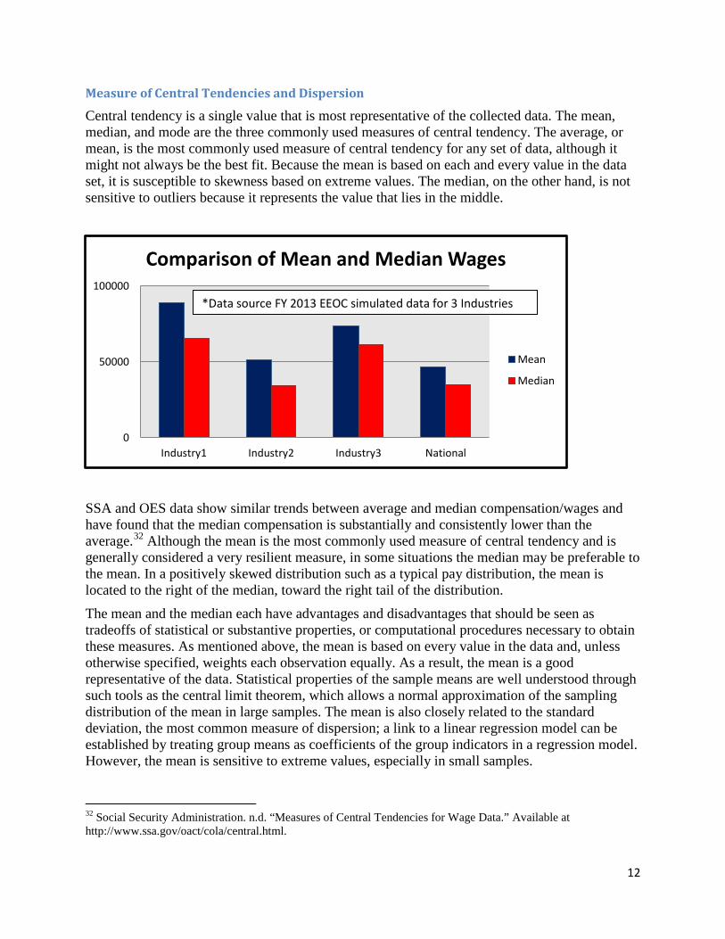
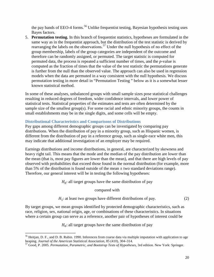
Central tendency is a single value that is most representative of the collected data. The mean, median, and mode are the three commonly used measures of central tendency. The average, or mean, is the most commonly used measure of central tendency for any set of data, although it might not always be the best fit. Because the mean is based on each and every value in the data set, it is susceptible to skewness based on extreme values. The median, on the other hand, is not sensitive to outliers because it represents the value that lies in the middle.

SSA and OES data show similar trends between average and median compensation/wages and have found that the median compensation is substantially and consistently lower than the average.32 Although the mean is the most commonly used measure of central tendency and is generally considered a very resilient measure, in some situations the median may be preferable to the mean. In a positively skewed distribution such as a typical pay distribution, the mean is located to the right of the median, toward the right tail of the distribution.

The mean and the median each have advantages and disadvantages that should be seen as tradeoffs of statistical or substantive properties, or computational procedures necessary to obtain these measures. As mentioned above, the mean is based on every value in the data and, unless otherwise specified, weights each observation equally. As a result, the mean is a good representative of the data. Statistical properties of the sample means are well understood through such tools as the central limit theorem, which allows a normal approximation of the sampling distribution of the mean in large samples. The mean is also closely related to the standard deviation, the most common measure of dispersion; a link to a linear regression model can be established by treating group means as coefficients of the group indicators in a regression model. However, the mean is sensitive to extreme values, especially in small samples.

32 Social Security Administration. n.d. “Measures of Central Tendencies for Wage Data.” Available at http://www.ssa.gov/oact/cola/central.html.

0

50000

100000

Industry1 Industry2 Industry3 National

Comparison of Mean and Median Wages

Mean

Median

*Data source FY 2013 EEOC simulated data for 3 Industries

12

On the other hand, the median may be a better indicator if the data values are skewed or have outlier(s). A generalization of median is to include auxiliary information that leads to the quantile regression model.33 The median, however, only uses the values in the middle of the data and does not reflect information in the tail of the distribution. Statistical inference for medians is more complicated than that for means. The version of the central limit theorem that can be used to obtain the normal distribution of the median in large samples depends on a complicated ancillary statistic that is difficult to estimate, and the missing data add to the difficulty.

Often, having both the mean and the median calculated and reported is best; however, doing so might considerably increase the burden on the agency. Although mean earnings data are consistently higher than the median, reflecting asymmetric distribution, they are the most reliable measure of central tendencies and, along with a measure of dispersion, will yield valuable information. If the standard deviation is collected along with the mean, then statistical inference for the mean will be possible using the standard results, such as Student’s t-distribution of the test statistic comparing the means of two samples.

A measure of dispersion provides a summary statistic that indicates the magnitude of the distribution dispersion. There are two different measures of dispersion: the range or interval measure, which is the difference between the two extreme values and interquartile range, and deviation, which is the average distance of the data points from the mean, such as variance, coefficient of variance, standard deviation, and median absolute deviation.

Range is the simplest to calculate; it is the difference between the two extreme values of the distribution. However, because the range calculation uses only the two extreme values of the data, it ignores a considerable amount of information. In continuous distributions with the tails extending to infinity (such as the earnings distributions), the range grows with the sample size and does not converge to any population quantity. Interquartile range is defined as the difference between the 25th and 75th percentile. Although interquartile range is not affected by extreme values (because it considers the middle 50 percent of the observations) and can be used as a measure of variability in open-ended distributions, it may be poorly defined in small samples, where its calculation depends on the working definitions of the percentiles.

Variance is defined as the average squared distance between the data values and the mean. Because variance is a symmetric function of the data points based on the sum across all data, it shares many conceptual properties, advantages, and disadvantages with the mean and therefore is also affected by outliers. Variance is the only measure of wage inequality that is amenable to an additive decomposition by sources, or factors, such as straight line pay versus bonuses versus the total value of benefits.34

One of the most commonly used measures of dispersion is the standard deviation. Standard deviation is the square root of the variance and, like variance, uses all the observations in a data set symmetrically and is sensitive to outliers. Interpretation of the standard deviation for skewed distributions may be complicated.

33 Koenker, R. 2005. Quantile Regression. Econometric Society Monographs, Cambridge University Press. 34 Shorrocks ,A.F. 1982. “Inequality Decomposition by Factor Components.” Econometrica 50(1), 193–211.

13

The coefficient of variation (CV) is the ratio of the standard deviation to the mean. Provided that the standard deviation and the mean are collected, CV can be easily computed. If a lognormal distribution of pay is implicitly assumed, then standard deviation of the residuals corresponds to the coefficient of variation of the distribution of pay. CV is a unit-free measure, and as such is relatively stable between groups that differ in mean pay. CV, however, relies on the collection of the standard deviation and the mean and also inherits sensitivity to outliers from the source statistics (mean and standard deviation).

Median absolute deviation (MAD) is the median of the absolute values of the deviations from the median. Although this measure is very robust to outliers for skewed populations, MAD treats the positive and negative deviations from the median differently; thus, its interpretation is complicated.

In a study published by BLS, authors Carl Barsky and Martin Personick compared the used index of dispersion and coefficient of variance to measure differences in the degree of wage dispersion among various industries.35 The index of dispersion was calculated by dividing the interquartile range (the difference between the third and first quartiles) by the median (second quartile). In this study the authors concluded that the dispersion measured by both methods was similar, and neither method changed the study’s result. However, they considered the coefficient of variation a more refined measurement because it is calculated based on each observation of the wage distribution, and no information is lost.

The measures of central tendency and dispersion reviewed above naturally fall into the moment-based measures (that is, those defined based on sums over all cases; mean, variance, and standard deviation) and order-statistics-based measures (median, range, interquartile range, MAD). The moment-based measures, as a rule, have statistical properties that are better understood; however, because they give extreme observations as much weight as observations in the middle of the range, moment-based measures are sensitive to outliers. The order-statistics-based measures, although more robust to outliers, are less frequently used in statistical practice. The fact that they use only a handful of observations around the required percentile (the 50th percentile for the median; the 25th and the 75th for the interquartile range) may be seen as a disadvantage in describing a whole demographic group in a given cell of the EEO form.

Computing or collecting the standard deviation or the coefficient of variance along with the mean will make statistical inference for the mean possible by using standard results such as Student’s t-distribution of the test statistic comparing the means of two samples.

Calculating Central Tendencies and Dispersion for Binned Data Many studies have been published that discuss the benefits and challenges of collecting interval data and the need for methodologies that can be applied to produce reliable summary estimates for such data sets. Several methods have been proposed for estimating the mean for interval data, including the arithmetic mean (midpoint) and geometric mean. Arithmetic mean is the sum of the upper and lower bound of each interval, divided by 2. OES previously used this method to estimate wage interval mean. Geometric mean is the product of upper and lower bound of the bin

35 Barsky, C.B., and M.E. Personick. 1981. “Measuring Wage Dispersion: Pay Ranges Reflect Industry Traits.” Monthly Labor Review 104, 35-41.

14

to the power of 1/2. In an article published by OES, the performance of these methodologies was compared, and the authors noted that all the methods performed well.36 In a 2005 study, Hozo et al. discussed methods to estimate mean and variance for interval data using the median, range, and sample size. The researchers showed that median can be used to estimate mean when the sample size is larger than 25. For smaller samples, they devised a new

formula, , that can be used to estimate the mean using the values of the median (m) and of the low and high end of the range (a and b, respectively). Range was also used to estimate the standard deviation. The study authors used estimators such as Range/4 for a normal distribution (the best estimator for the standard deviation and variance for sample sizes greater than 15 and less than 70), and Range/6 for any random distribution (for sample sizes above 70). For very small samples (up to 15), the best estimator was determined to be

, where a is the lower bound of the interval, b is the upper bound, and m is the median. 37

In another study published by BLS in 2009, Hesley and Duff found that O’Malley’s PQDE is a more effective method to generate occupational wage estimates than the current OES practice of using NCS data. The PQDE “has the advantage of being able to more fully use the information available in large quantities of interval data by considering both the proportions in the intervals and their relationship to adjacent intervals.” The researchers found that OES Intervals B through K “are adequately represented by the PQDE at the national major occupation group level of detail.” For the end intervals, some manipulations to the upper Interval L allow it “to be reasonably estimated using an exponential function of the estimator.” Interval A, the researchers note, requires additional research.38 Hesley and Duff compared the current OES method and the PQDE method by applying a new random group Jackknife variance estimator to both to calculate variance estimates on mean wages; they found that PDQE generated mean wages had a lower variance for 62 percent of the occupations.39

An exhaustive literature search did not show any applicable examples of the PQDE method being utilized for large data samples including applications for estimating sparse cell values. A detailed exploration of more applications of this method is outside the scope of this study. More information on the PDQE method is provided in Appendix A.

36 Kasturirangan et al. 2007. 37 Hozo, S.P., B. Djulbegovic, and I. Hozo. 2005. “Estimating the Mean and Variance From the Median, Range and the Size of a Sample.” BMC Medical Research Methodology 5(13), doi:10.1186/1471-2288-5-13. 38 Helsey and Duff 2009. 39 Helsey and Duff 2009, 1200.

15

Section II: Statistical Issues in the Analysis of Pay Disparities The following section reviews the appropriate earnings’ summaries for statistical analysis and testing. It concentrates on testing for pay disparities by protected target groups, such as those based on race, ethnicity, religion, gender, pregnancy status, national origin, age (40 or older), disability, or genetic information.

General Considerations The primary complication in establishing pay discrimination is that, in well-functioning economic systems, market forces determine one’s level of pay, and variation in pay is both necessary and inevitable. Employees who demonstrate higher productivity command higher wages because they produce more products or services for their employers and may have better outside opportunities. Federal legislation forbids discrimination in pay based on race, ethnicity, religion, sex (including pregnancy), national origin, age (40 or older), disability, or genetic information. In other words, although differences in pay that can be associated with the labor market characteristics of an employee are natural and necessary to bring labor markets into equilibrium and align the economic interests of employees and employers, the differences beyond these characteristics are less desirable and, in the case of differences that can be associated with protected groups, are prohibited.

Wage Equation as the Primary Tool To reflect this understanding in discussing pay discrimination, the Committee on National Statistics (CNSTAT) puts forward a popular model for labor income known in labor economics as the Mincer equation:

𝑙𝑙𝑙𝑙 𝑦𝑦𝑖𝑖 = 𝛽𝛽0 + 𝛽𝛽1′𝑑𝑑𝑖𝑖 + 𝛽𝛽2′𝑒𝑒𝑖𝑖 + 𝜀𝜀𝑖𝑖 (1)

where 𝑦𝑦𝑖𝑖 is the pay measure for individual 𝑖𝑖, 𝑑𝑑𝑖𝑖 is a vector of their design variables that indicate the demographic group, 𝑒𝑒𝑖𝑖 is a vector of control variables that can have a justifiable impact on difference in pay (such as education, certification, or work experience), 𝜀𝜀𝑖𝑖 is the regression error with zero mean and variance 𝜎𝜎2, and 𝛽𝛽1 and 𝛽𝛽2 are the vectors of regression coefficients. 40, 41 For an economic process that is characterized by no discrimination, 𝛽𝛽1 = 0; this is a statistical hypothesis that can be tested once the regression model (1) is estimated. Good notes that

[b]ecause of the complexity of the multiple regression model, it can be attacked on a variety of grounds:

• The data are incomplete or inaccurate. • Essential variables are omitted. • Tainted variables are included. • Distinct groups are wrongly aggregated in a single regression. • The model is not unique.

40 Mincer, J. 1974. Schooling, Experience, and Earnings. National Bureau of Economic Research. New York: Columbia University Press. 41 National Research Council 2012.

16

• The model is a poor predictor and thus inadequate or incorrect. • The wrong methodology is used to derive the coefficients. • The regression assumptions are not satisfied.42

Regression equation (1) works best in the context of large-scale data across multiple locations and industries. In the context of the data for a single establishment, the different demographic groups can be analyzed and contrasted with one another within that establishment. When the distribution of pay in a minority group (such as Hispanic women) is different from the distribution of pay in a reference group (such as single-race white men), this difference may indicate that an additional investigation may be required for this employer. Without explicitly accounting for the relevant control variables, however, meaningful comparisons between groups that can provide evidence of discrimination must be based on sufficiently narrow categories of job groups, occupations, and other variables determining the natural differences in pay. Good suggests that “in a discrimination case, the composition of the sample should be comparable (age, race, sex, years of experience) to that of the plaintiff… in all aspects but the one at issue.”43

CNSTAT argues that the best-fitting regression model should be chosen based on statistics such as Mallows’ 𝐶𝐶𝑝𝑝 or information criteria.44 Although this makes sense in many statistical applications because it reduces the number of degrees of freedom required to estimate all the model parameters, several issues are associated with model selection in the context of discrimination. First, reducing the degrees of freedom may not be a straightforward process, as discussed in “Degrees of Freedom” discussion below. Second, inference, including correctly determining standard errors and confidence intervals around predictions formed from selected models, needs to account for model uncertainty.45 Finally, both the design variables and the control variables play very specific and very distinct roles in equation (1). The design, or demographic, variables are included to test for discrimination, and omitting them from the model precludes conducting the required tests. The control variables are included to account for economically viable differences among industries, locations, job categories, and qualifications and certifications, among others. If these viable differences are related to the demographic variables — for example, specific locations that have unique demographic structures or certain demographic groups that have different education or certification profiles — then multicollinearity may drive the valid control variables to become insignificant, and if they are omitted from the model, the explanatory power is shifted to the demographic variable, creating the appearance of discrimination. Gastwirth cites the existing discrimination cases recommending that “regression analysis [does not need] to incorporate all measurable variables but should account for the major ones,” and gives example of cases in which model specifications that were too terse (for example, including only race and seniority without education or work experience) were deemed inadmissible in court.46 Some predictors may be

42 Good, P. 2001. Applying Statistics in the Courtroom: A New Approach for Attorneys and Expert Witnesses. Boca Raton, Florida: Chapman & Hall/CRC, 186. 43 Good 2001, 129. 44 Committee on National Statistics 2012. 45 Efron, B. 2014. “Estimation and Accuracy After Model Selection.” Journal of the American Statistical Association 109(507), 991–1006, with discussion and rejoinder, 1007–1022. 46 Gastwirth, J.L. 2000. “Issues Arising in the Use of Statistical Evidence in Discrimination Cases.” In: Gastwirth, J.L. (ed.), Statistical Science in the Courtroom. New York: Springer, 227–243.

17

treated with caution; for example, if minority employees with adequate qualifications are placed in lower-level jobs, then the job title variable suffers from the existing discriminatory practices that the statistical analysis is aimed at uncovering (that is, the explanatory variable is endogenous, in econometric terms) and therefore may not be a suitable regressor.47 To the extent possible, we would recommend retaining all the relevant variables as long as the sample sizes are sufficient; an often-used rule of thumb is to have 10 observations per parameter in the regression model.48 In discussing discrimination in hiring, Gastwirth writes, “As the defendant controls what information employment decisions and what data is preserved in its files, it is reasonable to assume that information on the important factors for on-the-job success are systematically obtained for all applicants or eligible employees and kept in their personnel records. This is why plaintiffs should consider all the job-related factors for which the employer has gathered data. If they do, then the employers should not be able to use information that was not obtained for all job candidates to rebut an inference derived from a statistical analysis using their complete files, since this would not give the plaintiffs a ‘full and fair opportunity’ to show pretext.”49 This advice clearly will be equally applicable to the study of compensation patterns.

Applicable Statistical Approaches When the regression approach cannot be used (for example, when no employee-level microdata are collected and aggregated data need to be used instead), other methods would need to be used instead. Because EEOC’s main task is measuring, interpreting, and testing pay disparities based on aggregate group-level measures, most of the statistical procedures discussed in this report are intended to identify differences between groups defined, for instance, by gender, race, and ethnicity, or a combination thereof. Several statistical approaches could be used:

1. Descriptive rankings. An investigator can sort business establishments by a chosen measure of pay inequality/dispersion and focus more in-depth analysis on those with the highest values of that measure. Such rankings, however, should be approached with caution. Similar procedures have been used in education research to identify the best-performing schools. Descriptive rankings would indicate that small schools often achieve the greatest gains in student performance. However, this result is simply an artifact of higher sampling variance due to lower sample size.50 Rankings may therefore need to be based on measures that are adjusted for measures of imprecision linked to the size of the establishment or to the sizes of the demographic cells within the establishment.

2. Frequentist modeling statistical inference. The data are assumed to come from an economic process, and outcomes such as pay are assumed to follow a specific distribution (such as normal, binomial, or lognormal). The measures of statistical uncertainty are derived by considering the outcomes to be random draws from these distributions. Distributions of statistics derived from the data, such as group means or regression coefficients, are obtained by appropriately aggregating over the distributions of the original outcomes. An investigator

47 Wooldridge, J. 2010. Econometric Analysis of Cross Section and Panel Data, 2nd edition. Cambridge, Massachusetts: MIT Press. 48 Long, J.S. 1997. Regression Models for Categorical and Limited Dependent Variables. Thousand Oaks, California: SAGE. 49 Gastwirth 2000. 50 Kane, T. J., and D. O. Staiger. 2002. The Promise and Pitfalls of Using Imprecise School Accountability Measures. Journal of Economic Perspectives, 16(4): 91-114.

18

then identifies the establishments that demonstrate pay gaps that are statistically significantly different from the assumed status quo value (such as zero, indicating no difference between groups) or from the population value, for example, by using an F-test based on regression (1). This is conceptually similar to what is currently being done using the data from EEO-1 forms to identify discriminatory practices in hiring.

3. Survey inference. The data are assumed to come from a fixed population. The measured characteristics of the observation units (employees’ demographics and pay) are assumed to be fixed quantities, and the only randomness is the result of taking random samples according to a prespecified probability sampling design. Many large scale labor statistics programs, such as the National Compensation Survey and Occupational Employment Statistics, rely on the data collected via a complex survey design. Within the existing data collection EEOC protocols, however, information is provided for all eligible employees of the establishment. Therefore, no sampling variability is present in the numerical summaries,, and as a result, there are always nonzero differences in pay among demographic groups (unless all employees work fixed hours for a fixed wage, such as the minimum wage, resulting in identical pay for each person). There are modifications of survey inference to bring it closer to the model-based frequentist inference as described above, in which the finite population at hand is assumed to have come from a statistical model.51,52 As the sample size approaches the population size, the sampling variability component shrinks to zero, leaving the model uncertainty as the leading term and reproducing the frequentist modeling results for the censuses of observation units. As with the frequentist approach, discrimination can be tested using a Wald F-test in the context of regression (1).

4. Bayesian inference. As with the frequentist paradigm, the data are assumed to be coming from an economic process, and outcomes are assumed to follow a specific distribution (such as normal, binomial, or lognormal). However, like the survey paradigm, the Bayesian paradigm treats the data as fixed, whereas the measures of uncertainty are associated with the knowledge, or lack thereof, of the parameters generating the data at hand. Without any data, knowledge about the parameters is described by a prior distribution of the parameter values. A vague prior may be used to indicate no knowledge whatsoever, whereas stronger priors that are more tightly concentrated near the parameter values known to be typical may reflect existing knowledge, such as that derived from prior studies, or the assumed situation, such as assuming no pay gaps. The observed data are then used to update the distribution of parameters and produce a posterior distribution through Bayes’ theorem.53 In the context of government statistics applications, Bayesian methods have been used very successfully to create synthetic microdata that protect the individual identity.54, 55 Special versions of these methods can be applied to create synthetic data sets for grouped income categories used in

51 Brewer, K. 2002. Combined Survey Sampling Inference: Weighing Basu’s Elephants. London: Arnold. 52 Demnati, A., and J.N.K. Rao. 2010. “Linearization Variance Estimators for Model Parameters From Complex Survey Data.” Survey Methodology 36(2), 193–202. 53 Gelman, A., and J.B. Carlin. 2013. Bayesian Data Analysis, 3rd edition. Boca Raton, Florida: Chapman and Hall/CRC. 54 Reiter, J.P. 2002. “Satisfying Disclosure Restrictions With Synthetic Data Sets.” Journal of Official Statistics 18(4), 531–543. 55 Drechsler, J. 2011. Synthetic Datasets for Statistical Disclosure Control. New York: Springer.

19

the pay bands of EEO-4 forms.56 Unlike frequentist testing, Bayesian hypothesis testing uses Bayes factors.

5. Permutation testing. In this branch of frequentist statistics, hypotheses are formulated in the same way as in the frequentist approach, but the distribution of the test statistic is derived by rearranging the labels on the observations.57 Under the null hypothesis of no effect of the group membership, labels of the group categories are independent of the outcome and therefore can be randomly assigned, or permuted. The target statistic is computed for permuted data, the process is repeated a sufficient number of times, and the p-value is computed as the fraction of times that the value of the test statistic the permutations generate is further from the null than the observed value. The approach can also be used in regression models when the data are permuted in a way consistent with the null hypothesis. We discuss permutation testing in more detail in “Permutation Testing ” below as it is a somewhat lesser known statistical method.

In some of these analyses, unbalanced groups with small sample sizes pose statistical challenges resulting in reduced degrees of freedom, wider confidence intervals, and lower power of statistical tests. Statistical properties of the estimates and tests are often determined by the sample size of the smallest group(s). For some racial and ethnic minority groups, the counts in small establishments may be in the single digits, and some cells will be empty.

Distributional Characteristics and Comparisons of Distributions Pay gaps among different demographic groups can be investigated by comparing pay distributions. When the distribution of pay in a minority group, such as Hispanic women, is different from the distribution of pay in a reference group, such as single-race white men, this may indicate that additional investigation of an employer may be required.

Earnings distributions and income distributions, in general, are characterized by skewness and heavy right tail. This means that the mode and the median of the pay distribution are lower than the mean (that is, most pay figures are lower than the mean), and that there are high levels of pay observed with probabilities that exceed those found in the normal distribution (for example, more than 5% of the distribution is found outside of the mean ± two standard deviations range). Therefore, our general interest will be in testing the following hypotheses:

𝐻𝐻0: all target groups have the same distribution of pay

compared with

𝐻𝐻1: at least two groups have different distributions of pay. (2)

By target groups, we mean groups identified by protected demographic characteristics, such as race, religion, sex, national origin, age, or combinations of these characteristics. In situations where a certain group can serve as a reference, another pair of hypotheses of interest could be

𝐻𝐻0: all target groups have the same distribution of pay

56 Heitjan, D. F., and D. B. Rubin. 1990. Inferences from coarse data via multiple imputation with application to age heaping. Journal of the American Statistical Association, 85 (410), 304–314. 57 Good, P. 2005. Permutation, Parametric, and Bootstrap Tests of Hypotheses, 3rd edition. New York: Springer.

20

compared with

𝐻𝐻1′ : at least one minority group has a distribution of pay that is different from the reference group. (3)

Because comparing full distributions is likely to be complicated and often relies on having precise pay measurements for each individual in the sample, some simplifications are often pursued, such as comparing distributions in terms of their means, medians, means + variances, or some other meaningful summaries. Direct testing of the equality of distributions of two or more groups, or summaries of these distributions, makes a very important implicit assumption that the groups are homogeneous with respect to the control variables. This assumption is relaxed when the regression approach based on wage equation (1) is being used. The standard test based on Mincer wage equations of labor economics is to test whether the demographic group is a significant predictor of the (differences in) log wages. Because regression models such as (1) deal with differences in (conditional) means, and that the log transformation converts differences in ratios into differences in the absolute levels of the transformed variable, this test checks for multiplicative differences between groups (such as whether females earn the same pay as males versus whether their pay is proportionally lower than that of males). In other words, rather than testing whether the distributions are identical, this test assumes that the distributions only differ by a multiplicative factor and tests for that specific aspect of the differences in distributions. Outside of regression models, comparisons between groups must be based on sufficiently narrow categories of job groups, occupations, and other variables that are associated with labor market characteristics determining the natural differences in pay.

Comparisons of Specific Aspects of the Pay Distribution The most common comparison of two samples is that of their means. In his comment on Vinod,58 Gastwirth shows that the difference in means is the natural expression of the overall economic advantage one group has over the other.59 For distributions that are approximately normal, a very common test is the t-test (sometimes referred to as the Welch t-test, as opposed to the original t-test by Student, which uses a pooled variance estimate)

𝑡𝑡 = 𝑦𝑦�1,𝑙𝑙1−𝑦𝑦�2,𝑙𝑙2

�𝑠𝑠12

𝑙𝑙1+𝑠𝑠22

𝑙𝑙2

(4)

that needs to be referred to the Student t-distribution with degrees of freedom,

𝜈𝜈 =�𝑠𝑠1

2

𝑙𝑙1+𝑠𝑠2

2

𝑙𝑙2�2

�𝑠𝑠12𝑙𝑙1

�2

𝑙𝑙1−1+�𝑠𝑠22𝑙𝑙2

�2

𝑙𝑙2−1

(5)

58 Vinod, H.D. 1985. “Measurement of Economics Distance Between Blacks and Whites.” Journal of Business and Economic Statistics 3(1), 78–88. 59 Gastwirth, J.L. (1985). “Comment on ‘Measurement of Economics Distance’ by H. D. Vinod.” Journal of Business and Economic Statistics 3(4), 405–407.

21

(see “Degrees of Freedom in Unbalanced Groups” for a discussion of degrees of freedom). 60 While the t-test compares only two groups, a generalization to multiple groups is provided by analysis of variance (ANOVA). The explicit expressions are omitted from this report, as this is a standard technique implemented in any statistical package.61 Generalizations of Satterthwaite’s formula (5) for degrees of freedom are also straightforward.

Another common comparison of distributions is in terms of their variances through Bartlett’s test:

𝑣𝑣 =(𝑙𝑙−𝑘𝑘) 𝑙𝑙𝑙𝑙 𝑆𝑆𝑝𝑝2−∑ �𝑙𝑙𝑗𝑗−1� 𝑙𝑙𝑙𝑙 𝑆𝑆𝑗𝑗

2𝑘𝑘𝑗𝑗=1

1+ 13(𝑘𝑘−1) �∑ 1

𝑙𝑙𝑗𝑗−1− 1𝑙𝑙−𝑘𝑘

𝑘𝑘𝑗𝑗=1 �

, 𝑙𝑙 = ∑ 𝑙𝑙𝑗𝑗 , 𝑆𝑆𝑝𝑝2 = 1𝑙𝑙−𝑘𝑘

∑ �𝑙𝑙𝑗𝑗 − 1�𝑆𝑆𝑗𝑗2, 𝑆𝑆𝑗𝑗2 = 1𝑙𝑙𝑗𝑗−1

∑ �𝑦𝑦𝑗𝑗𝑖𝑖 −𝑙𝑙𝑗𝑗𝑖𝑖=1

𝑘𝑘𝑗𝑗=1

𝑘𝑘𝑗𝑗=1

𝑦𝑦�𝑗𝑗�2(6),

presented here in the form appropriate for comparison of variances of k groups.

All of the t-tests, ANOVA, and especially the Bartlett variance tests are known to be sensitive to departures from normality. Johnson gave a correction for skewness of the one-sample t-test, and Cressie and Whitford proposed a two-sample generalization:

𝑢𝑢 = 𝑦𝑦�1,𝑙𝑙1−𝑦𝑦�2,𝑙𝑙2

�𝑠𝑠12

𝑙𝑙1+𝑠𝑠22

𝑙𝑙2

+ (𝐵𝐵1∗ − 𝐵𝐵2∗),

𝐵𝐵1∗ =

𝑏𝑏1𝑠𝑠13

6𝑙𝑙12�

𝑠𝑠12

𝑙𝑙1+𝑠𝑠22

𝑙𝑙2� +𝑏𝑏1𝑠𝑠1

3�𝑦𝑦�1,𝑙𝑙1−𝑦𝑦�2,𝑙𝑙2�2

3𝑙𝑙12�

𝑠𝑠12𝑙𝑙1

+𝑠𝑠22𝑙𝑙2

�2

�𝑠𝑠12

𝑙𝑙1+𝑠𝑠22

𝑙𝑙2

, 𝑏𝑏𝑗𝑗 =∑ �𝑦𝑦𝑗𝑗𝑊𝑊−𝑦𝑦�𝑗𝑗�

3𝑙𝑙𝑗𝑗𝑊𝑊=1

𝑠𝑠𝑗𝑗3 (7)

with 𝐵𝐵2∗ defined by flipping the sample indices 1 and 2 and 𝑏𝑏1, 𝑏𝑏2 being the estimates of skewness in the corresponding samples.62, 63 Interestingly, corrections for kurtosis are of a higher order, in that corrections for skewness have a greater effect in small samples. Cressie and Whitford also note that the preliminary test of equal variances that may lead to apparent simplification of the expression “was not helpful,” which supports the use of the Welch form (4) of the t-test.64 Also, in applying (7), note that the finite sample skewness and kurtosis have algebraic limits,65 which renders them only partially useful for small samples:

60 Satterthwaite, F.E. 1946. “An Approximate Distribution of Estimates of Variance Components.” Biometrics Bulletin 2(6), 110–114. 61 Rao, C.R. 2001. Linear Statistical Inference and Its Applications, 2nd ed. New York: Wiley. 62 Jonson, N. J. 1978. Modified t Tests and Confidence Intervals for Asymmetrical Populations. Journal of the American Statistical Association, 73 (363), 536–544. 63 Cressie, N.A.C., and H.J. Whitford. 1986. “How To Use the Two Sample t-Test.” Biometrical Journal 28(2), 131–148. 64 Cressie and Whitford 1986. 65 Cox, N.J. 2010. “The Limits of Sample Skewness and Kurtosis.” The Stata Journal 10(3), 482–495.

22

|𝑏𝑏| ≤ 𝑙𝑙−2√𝑙𝑙−1

. (8)

If the sample size is insufficient to produce an estimate of skewness comparable to the typical values of skewness observed elsewhere, then less biased and more stable estimates obtained from the population as a whole can be used.

Corrections for the nonnormal distribution can also be obtained through bootstrap or permutation approaches.66, 67 (The permutation approach is discussed below in “Permutation Testing .”) In the bootstrap approach, the reference distribution of the test statistic is obtained by sampling, with replacement, from the original data, and computing the statistic of interest for the resampled data. The data often need to be aligned to ensure that the data to be resampled satisfy the null hypothesis.68 Because there may be multiple ways to adjust the data, the problem can become fairly complicated. For example, if the mean level of pay is not equal between two groups, either the proportional/multiplicative change may be considered, or a shift (that is, an increase by a fixed number of dollars) can be considered.

Several economic measures intended to capture economic effects of inequality and discrimination have been proposed in the literature. Suppose that there are two groups to compare: the majority group (such as whites or males) and the minority group (such as other races or females), and their cumulative distribution functions (CDFs) are given by 𝐹𝐹𝑋𝑋(𝑒𝑒) and 𝐺𝐺𝑌𝑌(𝑦𝑦), respectively. Vinod defined the projected quantile estimated at 𝑦𝑦0 as

𝑦𝑦0∗ = 𝐹𝐹𝑋𝑋−1𝐺𝐺(𝑦𝑦0) (9)

and economic advantage at the income level of the disadvantaged group 𝑦𝑦0 as

𝐸𝐸𝐸𝐸[𝑒𝑒,𝑦𝑦|𝐺𝐺(𝑦𝑦0)] = 𝑦𝑦0∗ − 𝑦𝑦0.69 (10)

It can be integrated over a range of incomes, with integration over all possible incomes giving the difference in mean incomes as discussed by Gastwirth.70 Vinod demonstrated that defined in this way, the economic advantage of whites over blacks decreased in real terms between 1967 and 1979, especially among middle- and upper-middle-class income groups.

Butler and McDonald used partial moments

𝜙𝜙(𝑒𝑒;ℎ) = ∫ 𝑧𝑧ℎ𝑓𝑓(𝑧𝑧)𝑑𝑑𝑧𝑧 𝑥𝑥0

𝔼𝔼[𝑧𝑧ℎ] (11)

to define indices

66 Luh, W.-M., and J.H. Guo. 2000. “Johnson's Transformation Two-Sample Trimmed t and Its Bootstrap Method for Heterogeneity and Non-Normality.” Journal of Applied Statistics 27(8), 965–973. 67 Good 2005. 68 Hall, P., and S.R. Wilson. 1991. “Two Guidelines for Bootstrap Hypothesis Testing.” Biometrics 47(2), 757–762. 69 Vinod 1985. 70 Gatswirth 1985.

23

𝑃𝑃(𝑠𝑠, 𝑡𝑡) = 𝜙𝜙𝑌𝑌(𝜇𝜇𝑋𝑋 , 𝑠𝑠) − 𝜙𝜙𝑋𝑋(𝜇𝜇𝑌𝑌, 𝑡𝑡).71 (12)

In particular, 𝑃𝑃(0,0) = ℙ[𝑌𝑌 ≤ 𝜇𝜇𝑋𝑋]− ℙ[𝑋𝑋 ≤ 𝜇𝜇𝑌𝑌] is the difference between the fraction of the minority group with incomes less than the mean income of the majority group and the fraction for the majority group with incomes less than the mean income for the minority group, and 𝑃𝑃(1,1) = 𝔼𝔼[𝑌𝑌|𝑌𝑌 ≤ 𝜇𝜇𝑋𝑋]/𝜇𝜇𝑌𝑌 − 𝔼𝔼[𝑋𝑋|𝑋𝑋 ≤ 𝜇𝜇𝑌𝑌]/𝜇𝜇𝑋𝑋 is the difference between the fraction of total income of minority group with income less than the mean income of the majority group and the fraction of total income for the majority group with incomes less than the mean income for the minority group. Butler and McDonald introduced a social welfare function as the difference between aggregate utility functions for the two groups. When the utility is linear in incomes, the social welfare becomes 𝑃𝑃(0,0) + 𝑃𝑃(1,1) = 𝑃𝑃(0,1) + 𝑃𝑃(1,0).72 Fitting the generalized beta of the second kind (GB2) distribution to Current Population Survey (CPS) household data, they demonstrated decline in all four of these indices from 1948 to 1980 when comparing the incomes of whites and blacks. They also argued that P(0,0) may be the most relevant measure because of its clearer relation with concentration curves and Vinod’s quantile-based measures.73

The measures described above have been proposed in a descriptive sense of “making sense from a substantive economic perspective. The mathematical tradition of income inequality research is based on more stringent axiomatic approaches that involve principles such as the exchangeability of population members, principles of transfers (a transfer from a richer person to a poorer person cannot increase inequality), and homogeneity (a proportional increase in all incomes should have a proportional effect on dollar-denominated measures of inequality such as between-group differences, or no effect on scale-free measures such as the Gini index).74 Also, for the distance between two distributions, the standard axioms on the distance should apply (such as the property that the distance of the distribution to itself is zero, as well as the triangle inequality). Based on such axioms, Ebert arrives at a class of distances between income distributions given by

𝑑𝑑𝑟𝑟(𝑋𝑋,𝑌𝑌) = �∫ | 𝐹𝐹𝑋𝑋−1(𝑣𝑣) − 𝐺𝐺𝑌𝑌−1(𝑣𝑣)|𝑟𝑟𝑑𝑑𝑣𝑣10 �

𝑟𝑟, 𝑟𝑟 ≥ 1 .75 (13)

This measure simplifies to Vinod’s overall economic advantage when one of the income distributions is stochastically dominated by the other (see “Stochastic Dominance” below), so that the sign of 𝐹𝐹𝑋𝑋−1(𝑣𝑣) − 𝐺𝐺𝑌𝑌−1(𝑣𝑣) is the same for all 𝑣𝑣 ∈ (0,1).76

Parametric Distribution Modeling and Comparison If the error terms 𝜀𝜀𝑖𝑖 in regression model (1) are assumed to have a normal distribution, then the distribution of the pay measure 𝑦𝑦𝑖𝑖 is lognormal.77 In other words, if the differences in pay between different people are due to small multiplicative factors (for example, if person A is 15

71 Butler, R.J., and J.B. McDonald. 1987. “Interdistributional Income Inequality.” Journal of Business and Economic Statistics 5(1), 13–18. 72 Butler and McDonald 1987. 73 Vinod 1985. 74 Lambert, P.J. 1993. Distribution and Redistribution of Income: A Mathematical Analysis. New York: Manchester University Press. 75 Ebert, U. 1984. “Measures of Distance Between Income Distributions.” Journal of Economic Theory 32, 266–274. 76 Vinod 1985. 77 Aitchison, J., and J.A.C. Brown. 1957. The Lognormal Distribution. New York: Cambridge University Press.

24

percent more productive than person B when completing the same tasks), the lognormal distribution of the resulting wages would rise. The density of the lognormal distribution is given by

𝑙𝑙𝑙𝑙 𝑦𝑦 ∼ 𝑁𝑁(𝜇𝜇,𝜎𝜎2); 𝑓𝑓(𝑦𝑦; 𝜇𝜇,𝜎𝜎2) = 1𝑦𝑦𝑦𝑦√2𝜋𝜋

𝑒𝑒𝑒𝑒𝑒𝑒 �− (𝑙𝑙𝑙𝑙 𝑦𝑦−𝜇𝜇)2

2𝑦𝑦2� ,𝑦𝑦 > 0 , (14)

and its mean and variance are

𝔼𝔼𝑦𝑦 = 𝑒𝑒𝑒𝑒𝑒𝑒 �𝜇𝜇 + 𝑦𝑦2

2� ,𝕍𝕍𝑦𝑦 = [𝑒𝑒𝑒𝑒𝑒𝑒(𝜎𝜎2) − 1] 𝑒𝑒𝑒𝑒𝑒𝑒(2𝜇𝜇 + 𝜎𝜎2) . (15)

The grouped lognormal data can be analyzed using the CDF of this distribution, which can be easily found because of its relation to normal distribution:

𝐹𝐹(𝑦𝑦; 𝜇𝜇,𝜎𝜎2) = 𝛷𝛷(𝑙𝑙𝑙𝑙 𝑦𝑦−𝜇𝜇𝑦𝑦

). (16)

Within the context of the lognormal distribution, a popular alternative measure of dispersion is the coefficient of variation, defined as the ratio of the standard deviation of the distribution to its mean: CV 𝑦𝑦 = [exp(𝜎𝜎2) − 1]. Whereas the mean of the distribution can be measured in dollars and the variance in squared dollars, the coefficient of variation has no units and therefore is scale-free. Also, the correction by the mean allows for a meaningful comparison of the lognormal distributions that are known to only differ by scaling factors, such as inflation or location-based cost of living adjustments.

In practice, the lognormal distribution does not provide a sufficiently accurate fit to pay data. Of the other functional forms that have been proposed, one of the most general is the GB2.78 The density of GB2 distribution is given by

𝑓𝑓(𝑦𝑦;𝑎𝑎, 𝑏𝑏,𝑒𝑒, 𝑞𝑞) = 𝑎𝑎𝑦𝑦𝑎𝑎𝑝𝑝−1

𝑏𝑏𝑎𝑎𝑝𝑝𝐵𝐵(𝑝𝑝,𝑞𝑞)�1+�𝑦𝑦𝑏𝑏�𝑎𝑎�𝑝𝑝+𝑞𝑞 ,𝑦𝑦 > 0,𝑎𝑎, 𝑏𝑏,𝑒𝑒, 𝑞𝑞 > 0 , (17)

where 𝐵𝐵(𝑒𝑒, 𝑞𝑞) is the beta function

𝐵𝐵(𝑒𝑒, 𝑞𝑞) = ∫ 𝑡𝑡𝑝𝑝−110 (1 − 𝑡𝑡)𝑞𝑞−1 𝑑𝑑𝑡𝑡 = 𝛤𝛤(𝑝𝑝)𝛤𝛤(𝑞𝑞)

𝛤𝛤(𝑝𝑝+𝑞𝑞) , 𝛤𝛤(𝑧𝑧) = ∫ 𝑡𝑡𝑧𝑧−1+∞0 𝑒𝑒−𝑡𝑡 𝑑𝑑𝑡𝑡 .79 (18)

This distribution has absolute moments

𝔼𝔼𝑦𝑦𝑘𝑘 =𝑏𝑏𝑘𝑘𝐵𝐵(𝑝𝑝+𝑘𝑘𝑎𝑎,𝑞𝑞−𝑘𝑘𝑎𝑎)

𝐵𝐵(𝑝𝑝,𝑞𝑞) (19)

from which characteristics such as mean, variance, or inequality indices can be derived.80 It generalizes not only the beta distribution but also such distributions as the Dagum distribution81

78 McDonald, J.B. 1984. “Some Generalized Functions for the Size Distribution of Income.” Econometrica 55(3), 647–665. 79 Abramowitz, M., and I.A. Stegun. 1964. Handbook of Mathematical Functions. Washington, DC: National Bureau of Standards.

25

and the lognormal distribution implied by the Mincer equations (with 𝑎𝑎 → 0, 𝑞𝑞 → ∞ and 𝑏𝑏 = (𝜎𝜎2𝑎𝑎2)1/𝑎𝑎,𝑒𝑒 = 𝑎𝑎𝜇𝜇+1

𝑦𝑦2𝑎𝑎2, 𝑏𝑏 = 𝛽𝛽𝑞𝑞1/𝑎𝑎). To conduct an analysis with the banded data, the

distribution function was shown in McDonald to have a CDF given by

𝐹𝐹(𝑦𝑦;𝑎𝑎, 𝑏𝑏,𝑒𝑒, 𝑞𝑞) = ∫ 𝑓𝑓(𝑒𝑒;𝑎𝑎, 𝑏𝑏,𝑒𝑒, 𝑞𝑞)𝑑𝑑𝑒𝑒 =�

�𝑦𝑦𝑏𝑏�𝑎𝑎

1+�𝑦𝑦𝑏𝑏�𝑎𝑎�

𝑝𝑝

𝑝𝑝𝐵𝐵(𝑝𝑝,𝑞𝑞)𝑡𝑡0 2𝐹𝐹1 �𝑒𝑒, 1 − 𝑞𝑞;𝑒𝑒 + 1;

�𝑦𝑦𝑏𝑏�𝑎𝑎

1+�𝑦𝑦𝑏𝑏�𝑎𝑎� , (20)

where 2𝐹𝐹1(⋅) is the hypergeometric function

2𝐹𝐹1(𝑞𝑞, 𝑏𝑏; 𝑐𝑐; 𝑧𝑧) = ∑ (𝑞𝑞)𝑙𝑙(𝑏𝑏)𝑙𝑙(𝑐𝑐)𝑙𝑙

𝑧𝑧𝑙𝑙

𝑙𝑙!∞𝑙𝑙=0 , (𝑎𝑎)𝑙𝑙 = 𝑎𝑎(𝑎𝑎 + 1) … (𝑎𝑎 + 𝑙𝑙 − 1) .82 (21)

This function is notoriously difficult to compute in the general case, and approximations to it are known for their instability.

Once the parameters of statistical models describing the demographic groups are estimated, they can be compared using standard statistical tests based on the maximum likelihood estimates.83

Good warns that “forcing a statistical test to depend upon a specific distribution can result in bad choices.”84 As a body of empirical literature shows, a parametric modeling of income distributions may face the problem of poor fit. In their analysis of eight distributions (including six countries, with two countries analyzed separately in urban and rural areas), Hajargasht et al. found significant misfit in three out of eight cases, even for the most flexible GB2 distribution.85 In three out of five remaining cases, however, beta-2 distribution could be used instead, which is obtained from GB2 distribution by setting 𝑎𝑎 = 1.

Nonparametric Distribution Comparison When precise measurements are available for all units in the sample, nonparametric methods can be used as an alternative approach to comparing distributions between groups.86 These methods work with order statistics, ranks, or cumulative distribution functions without involving summary statistics such as means or variances. As a result, nonparametric methods achieve greater robustness for distributions that do not conform to the standard assumptions of t-tests or ANOVA, but this robustness generally comes at the expense of lower power (see Error Rates of Statistical Tests).

80 Jenkins, S. 2009. “Distributionally-Sensitive Inequality Indices and the GB2 Income Distribution.” Review of Income and Wealth 55(2), 392–398. 81 Dagum, C. 1977. “A New Model for Personal Income Distribution: Specification and Estimation.” Economie Appliquée 30, 413–443. 82 McDonald 1984. 83 Buse, A. 1982. “The Likelihood Ratio, Wald, and Lagrange Multiplier Tests: An Expository Note.” The American Statistician 36(3), 153–157. 84 Good 2001, 142. 85 Hajargasht, G., W.E. Griffiths, J. Brice, D.S. Prasada Rao, and D. Chotikapanich. 2012. “Inference for Income Distribution Using Grouped Data.” Journal of Business and Economic Statistics 30(4), 563–575. 86 Conover, W.J. 1999. Practical Nonparametric Statistics, 3rd edition. Hoboken, New Jersey: Wiley.

26

Several nonparametric tests exist to compare distributions between two groups. The Kolmogorov-Smirnov test compares the distribution functions between two groups, with the test statistic defined as

𝐷𝐷 = 𝑠𝑠𝑢𝑢𝑒𝑒 |𝐹𝐹1,𝑙𝑙1(𝑒𝑒) − 𝐹𝐹2,𝑙𝑙2(𝑒𝑒)|, 𝐹𝐹𝑘𝑘,𝑙𝑙𝑘𝑘(𝑒𝑒) = 1𝑙𝑙𝑘𝑘∑ 1{𝑒𝑒𝑖𝑖 ≤ 𝑒𝑒}𝑙𝑙𝑘𝑘𝑖𝑖=1 , (22)

where 𝐹𝐹𝑘𝑘,𝑙𝑙𝑘𝑘(𝑒𝑒) is the cumulative distribution function in group 𝑘𝑘, and the subindices are used to highlight the dependence on the sample size. The test rejects the null hypothesis of equality of

the two distributions when 𝐷𝐷 > 𝑐𝑐(𝛼𝛼)�𝑙𝑙1+𝑙𝑙2𝑙𝑙1𝑙𝑙2

, and 𝑐𝑐(𝛼𝛼) is a calibration constant based on the size

of the test, 𝑐𝑐(𝛼𝛼) = 1.36 for 𝛼𝛼 = 0.05. This test is most sensitive to the departures in the middle part of the distribution, which can be viewed as an advantage in the current application. It is not very sensitive to the outliers at the tails of the distribution and deals with most of the population in the middle of it. Although the Kolmogorov-Smirnov test is applicable to the two-group comparisons, such as comparing males and females, it does not allow generalizations for multiple groups, such as multiple racial categories or the interaction between gender and race. The Kolmogorov-Smirnov test assumes independence between the CDFs being compared and does not perform well when the distributions being compared are based on parametric functional forms with estimated parameters.

A popular two-sample nonparametric test to compare two populations is the two-sample Wilcoxon rank-sum test, which is equivalent to Mann-Whitney two-sample test. The underlying population parameter of the Wilcoxon-Mann-Whitney test is the probability that a randomly selected observation from group 1 is greater than a randomly selected observation from group 2.87, 88 Gastwirth argues that this parameter can be a useful supplement to the difference in means underlying the t-test and a relevant policy parameter in itself.89, 90 Implementations in R package incorrectly identify the alternative hypothesis of the test as that of a nonzero shift. Although the test is sensitive to pure shifts, it has the more general interpretation of a test of the differences between two or more distributions. To form the Wilcoxon test statistic, the two samples are pooled, the observations are sorted to produce ranks, and the test statistic, with reference to the first group, is 𝑇𝑇 = ∑ 𝑅𝑅1𝑖𝑖

𝑙𝑙1𝑖𝑖=1 , where 𝑅𝑅1𝑖𝑖 is the rank of the 𝑖𝑖-th observation from the first sample. It

has an asymptotic normal distribution with mean 𝑙𝑙1(𝑙𝑙1 + 1)/2 and variance 𝑙𝑙1𝑙𝑙2(𝑙𝑙1 + 𝑙𝑙2 +1)/12, giving rise to a 𝑧𝑧-statistic. The Mann-Whitney 𝑈𝑈-statistic is the number of times in all pairwise comparisons that an observation from the second group is less than an observation from the first group: 𝑈𝑈 = ∑ ∑ 1�𝑋𝑋2𝑗𝑗 < 𝑋𝑋1𝑖𝑖�𝑗𝑗𝑖𝑖 . For the two-sample comparisons problem, the two statistics only differ by a constant: 𝑈𝑈 = 𝑇𝑇 − 𝑙𝑙1(𝑙𝑙1 + 1)/2. The later analyses in this report utilize this asymptotic approximation; for smaller samples, exact 𝑒𝑒-values can be utilized. Gibbons and Chakaborti91 note that “[the asymptotic] approximation has been found reasonably

87 Gastwirth, J.L. 1975. “Statistical Measures of Earnings Differentials.” The American Statistician 29(1), 32–35 88 Conroy, R.M. 2012. “What Hypotheses Do ‘Nonparametric’ Two-Group Tests Actually Test?” The Stata Journal 12(2), 182–190. 89 Gastwirth 1975. 90 Gastwirth 1985. 91 Gibbons, J. D., and S. Chakraborti. 2011. Nonparametric Statistical Inference, 5th edn. Boca Raton, FL: Chapman & Hall/CRC.

27

accurate for equal sample sizes as small as 6”. The exact 𝑒𝑒-values are computationally

demanding as they require a recursive enumeration of at least 𝛼𝛼 �𝑙𝑙1 + 𝑙𝑙2𝑙𝑙1

� orderings of the observations from the two samples, where 𝛼𝛼 is the target significance level. This number becomes very large very quickly, with little accuracy gains on top of the asymptotic expression in large samples.

There also exists a more straightforward non-parametric analogue of the 𝑡𝑡-test: rather than a test of two means, the medians of the two groups are explicitly compared. This test, however, is known to have a power that is much lower than other applicable tests, especially in small samples, which makes it difficult to recommend for the current practical application.92

Rosenbaum introduced the concept of sensitivity analysis, in which the differences in the observed outcomes between two groups are attributed to the different prevalence of an unobserved (unmeasured) factor 𝑈𝑈 in these groups.93, 94 Sensitivity analysis then aims to obtain the bounds on the ratio 𝛤𝛤 of the prevalences of 𝑈𝑈 in these groups that would fully explain the observed differences in the outcomes. Gastwirth explains this approach in context of discrimination as follows: Let the success rates of the majority and minority groups be 𝑒𝑒1 and 𝑒𝑒2, respectively, and the prevalence of the unmeasured factor 𝑈𝑈 in these groups, 𝑓𝑓1 and 𝑓𝑓2, respectively.95 Let the observed relative risk be 𝑅𝑅𝑜𝑜 = 𝑒𝑒2/𝑒𝑒1 (that is, by how much the majority success rate exceeds that of the minority). Then, for a given value of the relative risk 𝛤𝛤 = 𝑅𝑅𝑢𝑢 associated with the factor 𝑈𝑈 (that is, the relative increase in the success rate between otherwise identical individuals that differ only in the presence of this factor), the prevalence of 𝑈𝑈 in the minority group must be at least 𝑓𝑓2 ≥ 𝑅𝑅0𝑓𝑓1 + 𝑅𝑅0−1

𝑅𝑅𝑢𝑢−1 for the presence 𝑈𝑈 to explain the observed

differences in success rates. In the most conservative case, if 𝑅𝑅𝑢𝑢 = +∞ (meaning that the presence of 𝑈𝑈 makes a person arbitrarily more attractive for hire) and 𝑓𝑓1 = 1 (that is, everybody in the majority population has the trait 𝑈𝑈), then if at least 𝑓𝑓2 × 100% of the minority population have 𝑈𝑈, this factor could not reduce the disparity to insignificance.

For continuous data, such as pay levels, Rosenbaum notes that extensions are possible for continuous outcomes when the test statistic has the functional form 𝑇𝑇 = ∑ 𝑍𝑍𝑖𝑖𝑞𝑞𝑖𝑖𝑙𝑙

𝑖𝑖=1 , where 𝑍𝑍𝑖𝑖 is the “treatment” (minority group) indicator and 𝑞𝑞𝑖𝑖 is a function of the response (for example, ranks of the pay levels in Wilcoxon test statistic) and is asymptotically normal, so that a one-sided hypothesis has a critical region 𝑇𝑇 ≥ 𝑘𝑘 for some 𝑘𝑘.96, 97 This approach is implemented in the rbounds package in R.98

92 Freidlin, B., and J.L. Gastwirth. 2000. “Should the Median Test Be Retired from General Use?” The American Statistician 54(3), 161–164. 93 Rosenbaum, P.R. 1987. “Sensitivity Analysis for Certain Permutation Inferences in Matched Observational Studies.” Biometrika 74(1), 13–26. 94 Rosenbaum, P.R. 2002. Observational Studies, 2nd ed. New York: Springer. 95 Gastwirth 2000. 96 Rosenbaum 1987. 97 Rosenbaum 2002, 140–148. 98 Keele, L. J. 2014. “rbounds: Perform Rosenbaum Bounds Sensitivity Tests for Matched and Unmatched Data.” R package, version 2.1. Available at http://cran.r-project.org/web/packages/rbounds/.

28

A multigroup nonparametric comparison can be conducted using the Kruskal-Wallis test, which is a one-way analysis of variance for ranks of observations within the pooled data set. If the null hypothesis of the Kruskal-Wallis test is rejected, then at least one group stochastically dominates at least one other group. In other words, the CDF of the dominating group lies to the right, or below, the CDF of the dominated group.

Stochastic Dominance As discussed later in “Analyses with the Group-Level Data,” much of the research into the methodology of grouped income data that has been accumulated in distribution economics deals with estimation of the shape of income distribution from reported aggregates at quintile or decile levels. On most occasions, income distribution economists are interested in normalized measures of inequality concerned with within-group inequality. These measures are often based on the Lorenz curve, which is a reparameterization of income distribution.99 The abscissa of the Lorenz curve shows the cumulative proportion of the population ordered by income, and the ordinate shows the cumulative proportion of income this lower part of the population has:

𝐿𝐿(𝑒𝑒) = ∫ 𝑥𝑥 𝑓𝑓(𝑥𝑥)𝜇𝜇

𝑑𝑑𝑒𝑒 , 𝐿𝐿(0) = 0, 𝐿𝐿(1) = 1𝐹𝐹−1(𝑝𝑝)0 . (23)

For example, the point (0.20, 0.03) would mean that the poorest 20 percent of the population together receive 3 percent of the total income. Figure 1 shows the Lorenz curve based on CPS data. It has a typical convex shape, starting with a certain proportion of zero incomes and sloping upwards. The line of perfect equality is the diagonal line, and twice the area between that line and Lorenz curve is a popular inequality measure, the Gini index.

99 Lambert 1993.

29

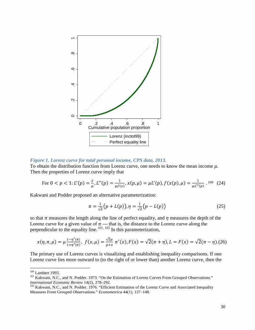
Figure 1. Lorenz curve for total personal income, CPS data, 2013. To obtain the distribution function from Lorenz curve, one needs to know the mean income 𝜇𝜇. Then the properties of Lorenz curve imply that

For 0 < 𝑒𝑒 < 1: 𝐿𝐿′(𝑒𝑒) = 𝑥𝑥𝜇𝜇

, 𝐿𝐿′′(𝑒𝑒) = 1𝜇𝜇𝑓𝑓(𝑥𝑥) , 𝑒𝑒(𝑒𝑒, 𝜇𝜇) = 𝜇𝜇𝐿𝐿′(𝑒𝑒),𝑓𝑓(𝑒𝑒(𝑒𝑒), 𝜇𝜇) = 1

𝜇𝜇𝐿𝐿′′(𝑝𝑝) . 100 (24)

Kakwani and Podder proposed an alternative parameterization:

𝜋𝜋 = 1√2�𝑒𝑒 + 𝐿𝐿(𝑒𝑒)�,𝜂𝜂 = 1

√2�𝑒𝑒 − 𝐿𝐿(𝑒𝑒)� (25)

so that 𝜋𝜋 measures the length along the line of perfect equality, and 𝜂𝜂 measures the depth of the Lorenz curve for a given value of 𝜋𝜋 — that is, the distance to the Lorenz curve along the perpendicular to the equality line.101, 102 In this parameterization,

𝑒𝑒(𝜂𝜂,𝜋𝜋, 𝜇𝜇) = 𝜇𝜇 1−𝜂𝜂′(𝜋𝜋)1+𝜂𝜂′(𝜋𝜋) , 𝑓𝑓(𝑒𝑒, 𝜇𝜇) = √2𝜇𝜇

𝜇𝜇+𝑥𝑥 𝜋𝜋′(𝑒𝑒),𝐹𝐹(𝑒𝑒) = √2(𝜋𝜋 + 𝜂𝜂), 𝐿𝐿 = 𝐹𝐹(𝑒𝑒) = √2(𝜋𝜋 − 𝜂𝜂).(26)

The primary use of Lorenz curves is visualizing and establishing inequality comparisons. If one Lorenz curve lies more outward to (to the right of or lower than) another Lorenz curve, then the

100 Lambert 1993. 101 Kakwani, N.C., and N. Podder. 1973. “On the Estimation of Lorenz Curves From Grouped Observations.” International Economic Review 14(2), 278–292. 102 Kakwani, N.C., and N. Podder. 1976. “Efficient Estimation of the Lorenz Curve and Associated Inequality Measures From Grouped Observations.” Econometrica 44(1), 137–148.

0.2

.4.6

.81

0 .2 .4 .6 .8 1Cumulative population proportion

Lorenz (inctot99)Perfect equality line

30

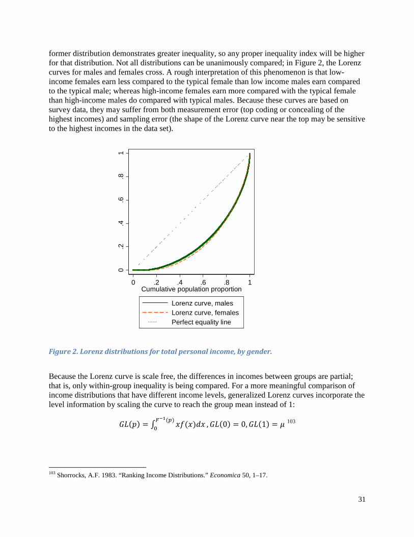
former distribution demonstrates greater inequality, so any proper inequality index will be higher for that distribution. Not all distributions can be unanimously compared; in Figure 2, the Lorenz curves for males and females cross. A rough interpretation of this phenomenon is that low-income females earn less compared to the typical female than low income males earn compared to the typical male; whereas high-income females earn more compared with the typical female than high-income males do compared with typical males. Because these curves are based on survey data, they may suffer from both measurement error (top coding or concealing of the highest incomes) and sampling error (the shape of the Lorenz curve near the top may be sensitive to the highest incomes in the data set).

Figure 2. Lorenz distributions for total personal income, by gender.

Because the Lorenz curve is scale free, the differences in incomes between groups are partial; that is, only within-group inequality is being compared. For a more meaningful comparison of income distributions that have different income levels, generalized Lorenz curves incorporate the level information by scaling the curve to reach the group mean instead of 1:

𝐺𝐺𝐿𝐿(𝑒𝑒) = ∫ 𝑒𝑒𝑓𝑓(𝑒𝑒)𝑑𝑑𝑒𝑒𝐹𝐹−1(𝑝𝑝)0 ,𝐺𝐺𝐿𝐿(0) = 0,𝐺𝐺𝐿𝐿(1) = 𝜇𝜇 103

103 Shorrocks, A.F. 1983. “Ranking Income Distributions.” Economica 50, 1–17.

0.2

.4.6

.81

0 .2 .4 .6 .8 1Cumulative population proportion

Lorenz curve, malesLorenz curve, femalesPerfect equality line

31

Figure 3 depicts the generalized Lorenz curves based on the CPS data, with the curve for males above that for females.

Figure 3. Generalized Lorenz curves for the total personal income, by gender.

Generalized Lorenz curves have an important relation to the concept of stochastic dominance. For two distributions 𝐹𝐹(𝑒𝑒) and 𝐺𝐺(𝑦𝑦), the following three statements are equivalent:

1. For all 0 < 𝑒𝑒 < 1,𝐹𝐹−1(𝑒𝑒) ≥ 𝐺𝐺−1(𝑒𝑒), that is, the cumulative distribution of 𝐹𝐹(⋅) lies to the right of the CDF of 𝐺𝐺(⋅).

2. For all increasing strictly concave utility functions, ∫ 𝑈𝑈(𝑒𝑒)𝑓𝑓(𝑒𝑒)d𝑒𝑒 ≥ ∫ 𝑈𝑈(𝑦𝑦)𝑔𝑔(𝑦𝑦)d𝑦𝑦, where 𝑓𝑓(𝑒𝑒) and 𝑔𝑔(𝑦𝑦) are the pdf functions of the two distributions; that is, the social welfare is unanimously higher for distribution 𝐹𝐹(⋅).

3. For all 0 < 𝑒𝑒 < 1, 𝐺𝐺𝐿𝐿𝐹𝐹(𝑒𝑒) ≥ 𝐺𝐺𝐿𝐿𝐺𝐺(𝑒𝑒), that is, the generalized Lorenz curve for 𝐹𝐹(⋅) lies above that of 𝐺𝐺(⋅).

This means that the generalized Lorenz curves provide a compact visual representation of the stochastic dominance of one distribution over another. For the applications in the current project, the Lorenz curve can be reconstructed from the grouped data — and the generalized Lorenz curve can be obtained by multiplying the Lorenz curve by the group mean income — for an EEOC investigator to review whether the demographic groups have stochastic dominance relations with one another.

Mean male income = $45189

Mean female income = $27064

010

000

2000

030

000

4000

050

000

Gen

. Lor

enz

(inct

ot99

)

0 .2 .4 .6 .8 1Cumulative population proportion

Gen. Lorenz curve, malesGen. Lorenz curve, females

32

Permutation Testing Permutation testing represents a simulation-based approach to frequentist statistical hypothesis testing.104 In this approach, the distribution of the chosen test statistics is explicitly created by simulating from the existing data upon imposing the null hypothesis. For tests of equality between groups, this approach boils down to scrapping the existing labels of the categorical variables and assigning the labels randomly, as the null hypothesis of no differences implies. Alternatively, the values of the outcome can be randomly assigned to the observations within groups defined by control variables. The target statistic is computed for permuted data, the process is repeated sufficiently many times, and the p-value is computed as the fraction of times the value of the test statistic generated by the permutations is further from the null than the observed value. The process and the results can be easily visualized with a histogram of the simulated values of the test statistic with the observed value overlaid. Permutation tests are exact in that they do not rely on any large-sample approximations, although Monte Carlo simulation error may present (and is quantifiable). Some of the parametric tests, such as the test for equal means of two groups, are asymptotically equivalent to permutation procedures; if that is the case, the permutation test is usually as powerful as the most powerful parametric test.

Permutation tests can be modified to account for covariates known to affect the outcome using the approach of conditional permutations, or restricted randomization.105 In this approach, permutations of the design variable labels, such as race or gender, can be made within the groups defined by the control variables, such as job categories. Justification of the conditional permutation requires assumptions similar to those found in the literature on impact evaluation, such as conditional independence, or selection on observables; the observed demographic category of an individual 𝑖𝑖 and the vector of potential outcomes (levels of pay for that individual should that individual belong to a different demographic group) are conditionally independent given the control variables (such as job categories).

Analysis with Grouped Data Within Firm Because we recommend collecting pay data by bands within the target groups (see Section I), we will also need to analyze the data in bands rather than exact measurements of the level of pay. Several options are available:

1. The data can be analyzed as a contingency table, with the demographic groups as the table’s columns and pay bands as rows, ignoring the ordinal relations between the pay bands. This approach is the most conservative in that it makes the fewest assumptions about the underlying pay data.

2. Nonparametric rank-based tests can be applied to the grouped data, retaining the information regarding the relative ordering of the levels but ignoring the specific cutoff values associated with a given band.

104 Good 2005. 105 Rosenbaum, P.R. 1984. “Conditional Permutation Tests and the Propensity Score in Observational Studies.” Journal of the American Statistical Association 79(387), 565–574.

33

3. A median regression model can be fit instead of the conditional mean model (estimated by ordinary least squares). Median regression is a version of quantile regression that models a specific quantile of the conditional distribution.106

4. By making an assumption of an underlying normal or lognormal distribution, an interval regression model can be fit to the grouped data.107, 108 Unlike other approaches that effectively assume that employees in the same pay band are paid the same amount, interval regression explicitly models the distribution within the pay band.

5. Rosenbaum’s sensitivity analysis continues to be applicable, although subject to the caveats regarding performance of Wilcoxon test with grouped data (ties).109

Compared with the analysis of the original data with accurate pay amounts, the Mann-Whitney-Wilcoxon test with grouped data is still applicable but will suffer from the presence of ties.110 Ties are observations with identical values. When the underlying variable is a truly continuous one, all ranks are unique. However, when the underlying variable is only an ordinal one, identical values (i.e., workers in the same pay band) are likely to be found in the data in one or more groups being compared. When ties are present, the exact computation of 𝑒𝑒-values for small samples becomes infeasible, and the test has to rely on asymptotic approximation. Implementing the test requires that (a) the test statistic accounts for ties properly (such as by incrementing the Mann-Whitney 𝑈𝑈-statistic by 0.5 when the observations are tied), and (b) the variance is corrected for ties: 𝕍𝕍[𝑈𝑈] = 𝑙𝑙1𝑙𝑙2(𝑙𝑙1+𝑙𝑙2+1)

12{1 − ∑𝑡𝑡�𝑡𝑡2−1�

(𝑙𝑙1+𝑙𝑙2)[ (𝑙𝑙1+𝑙𝑙2)2−1]} where 𝑡𝑡 is the multiplicity of a tie, and the summation is over all sets of ties. Software packages typically either default to these modifications when ties are encountered or provide options for analysis with ties.

Power of the MWW test has been discussed by Noether111: the power of a one-sided MWW test is given by

𝑃𝑃𝑃𝑃𝑃𝑃𝑒𝑒𝑟𝑟 = 𝑃𝑃𝑟𝑟𝑃𝑃𝑏𝑏 �𝑍𝑍 > 𝜇𝜇0(𝑇𝑇)−𝜇𝜇1(𝑇𝑇)𝜌𝜌𝑦𝑦0(𝑇𝑇) + 𝑧𝑧𝛼𝛼

𝜌𝜌�, (27)

where 𝜇𝜇0(𝑇𝑇) and 𝜇𝜇1(𝑇𝑇) are the means of the sampling distribution under the null and under the alternative, respectively; 𝜎𝜎02(𝑇𝑇) is the variance of the test statistic under the null; 𝜌𝜌 =𝜎𝜎1(𝑇𝑇)/𝜎𝜎0(𝑇𝑇) is the ratio of the standard deviations of the sampling distributions of the test statistics under the null and the alternative, usually assumed to be 1 when the distributions are sufficiently close; and 𝑧𝑧𝛼𝛼 is the upper 𝛼𝛼-level significance point. The Mann-Whitney test statistic 𝑈𝑈 has the mean 𝑙𝑙1𝑙𝑙2𝑒𝑒′, where 𝑒𝑒′ = Prob[𝑌𝑌2𝑖𝑖 > 𝑌𝑌1𝑖𝑖] + 1

2Prob[𝑌𝑌2𝑖𝑖 = 𝑌𝑌1𝑖𝑖]. Under the null of equal

106 Koenker, R. 2005. Quantile Regression. Econometric Society Monographs, no. 38. New York: Cambridge University Press. 107 McCullagh, P. 1980. “Regression Models for Ordinal Data.” Journal of the Royal Statistical Society, Series B: Methodology 42(2), 109–142. 108 Stewart, M.B. 1983. “On Least Squares Estimation When the Dependent Variable Is Grouped.” Review of Economic Studies 50(4), 737. 109 Rosenbaum 2002, 140–144. 110 Gibbons, J. D., and S. Chakraborti. 2011. 111 Noether, G. E. (1987). Sample Size Determination for Some Common Nonparametric Tests. Journal of the American Statistical Association, 82 (398), 645–647.

34

earnings distributions (no discrimination), 𝑒𝑒′ = 1/2. The value of this parameter under alternatives depends on both the degree of discrimination, and the groupings used.

Median regression is a variant of linear regression in which the focus is on the conditional quantiles of the distribution 𝑦𝑦𝑖𝑖|𝑒𝑒𝑖𝑖, such as, the conditional median 𝐹𝐹𝑦𝑦𝑊𝑊|𝑥𝑥𝑊𝑊

−1(1/2), rather than the conditional mean 𝔼𝔼[𝑦𝑦𝑖𝑖|𝑒𝑒𝑖𝑖]. Initially proposed as a variant of a regression method robust to outliers, quantile regression has become a widely used econometric tool to study distributional impacts.112 While applicable with Mincer wage equation (1), quantile regression appears to be a promising method for grouped data to model the median income group into which individuals with different demographic characteristics fall. Unfortunately, the straightforward application of median regression with simulated data produced unsatisfactory results (see “Simulated EEOC data”). When the outcome variable in the median regression is the sequential number of the pay band, then the coefficient estimates are integer numbers (zero if the median pay of a demographic group is the same as that of the reference group, –1 if it the median pay group for a demographic group is the next lowest pay band, and so on). A greater complication involves standard errors, which are calculated by comparing the conditional sample median with its nearby observations within a demographic group. However, if the dependent variable does not vary in the neighborhood of the median (all cases with incomes near the median are contained in the same pay group and therefore have the same value of the left-hand-side variable), then the standard error is zero, making statistical inference impossible. In other words, a violation of the assumption that the dependent variable is continuous may render the quantile regression method inapplicable.

The interval regression model incorporates measurement error in measuring the true pay level into the regression model (1) by explicitly assuming the normal distribution of the error terms 𝜖𝜖𝑖𝑖of the model for the log pay. Then the probability of an event that an individual 𝑖𝑖 has income between 𝑎𝑎𝑖𝑖 and 𝑏𝑏𝑖𝑖 is

ℙ [ 𝑦𝑦𝑖𝑖 ∈ (𝑎𝑎𝑖𝑖, 𝑏𝑏𝑖𝑖)] = ℙ[𝑙𝑙𝑙𝑙 𝑎𝑎𝑖𝑖 < 𝛽𝛽0 + 𝛽𝛽1′𝑑𝑑𝑖𝑖 + 𝛽𝛽2′𝑒𝑒𝑖𝑖 + 𝜖𝜖𝑖𝑖 < 𝑙𝑙𝑙𝑙 𝑏𝑏𝑖𝑖] = = ℙ[𝑙𝑙𝑙𝑙 𝑎𝑎𝑖𝑖 − 𝛽𝛽0 − 𝛽𝛽1′𝑑𝑑𝑖𝑖 − 𝛽𝛽2′𝑒𝑒𝑖𝑖 < 𝜖𝜖𝑖𝑖 < 𝑙𝑙𝑙𝑙 𝑏𝑏𝑖𝑖 − 𝛽𝛽0 − 𝛽𝛽1′𝑑𝑑𝑖𝑖 − 𝛽𝛽2′𝑒𝑒𝑖𝑖] =

=𝛷𝛷 �𝑙𝑙𝑙𝑙𝑏𝑏𝑊𝑊−𝛽𝛽0−𝛽𝛽1′𝑑𝑑𝑊𝑊−𝛽𝛽2′𝑥𝑥𝑊𝑊

𝑦𝑦� − 𝛷𝛷 �𝑙𝑙𝑙𝑙𝑎𝑎𝑊𝑊−𝛽𝛽0−𝛽𝛽1

′𝑑𝑑𝑊𝑊−𝛽𝛽2′𝑥𝑥𝑊𝑊𝑦𝑦

� , (28)

where Φ(𝑧𝑧) is the distribution function of a standard normal variable. Note that the normality assumption pertains to the distribution of log incomes within a demographic group defined by regressors 𝑒𝑒𝑖𝑖. Within a pay band, the distribution of the log-pay is truncated normal. Note also that because of the log normality assumption, the boundaries of the group are defined in log terms. With the individual-level data, the model can be estimated by maximum likelihood assuming independence of observations, in which case the overall likelihood is the product of such contributions. With the group-level data, these contributions need to be weighted by frequency weights — that is, the counts of the number of employees in each cell. The interpretation of coefficients and tests based on them is going to be the same as for the linear regression case. Note that the interval regression model produces an estimate of variance 𝜎𝜎�,

112 Bassett, G., and R. Koenker. 1978. “Asymptotic Theory of Least Absolute Error Regression.” Journal of the American Statistical Association 73(363), 618–622.

35

which can be used if means but not variances are collected. (For an extensive treatment of this interval regression model, see Cameron and Triverdi.113) In the current application, the bounds 𝑎𝑎𝑖𝑖 and 𝑏𝑏𝑖𝑖 are fixed by the design: 𝑎𝑎𝑖𝑖 ∈ {𝑧𝑧0 = 0, 𝑧𝑧1, 𝑧𝑧2, … , 𝑧𝑧𝐾𝐾−1}, 𝑏𝑏𝑖𝑖 ∈ {𝑧𝑧1, 𝑧𝑧2, … , 𝑧𝑧𝐾𝐾−1, 𝑧𝑧𝐾𝐾 = +∞), so if 𝑚𝑚𝑖𝑖 is the consecutive number of the pay band of individual 𝑖𝑖, then 𝑎𝑎𝑖𝑖 = 𝑧𝑧𝑚𝑚𝑊𝑊−1, 𝑏𝑏𝑖𝑖 = 𝑧𝑧𝑚𝑚𝑊𝑊 .

Analysis with Grouped Data Between Firms While the above methods of ordinal grouped data are applicable to the analysis of pay disparities based on firm microdata, other aggregated analyses may be of interest for the purposes of conducting an initial investigation into an establishment. EEOC has extensive experience in investigation of hiring practices, where it uses two-way contingency tables with the protected group status as one of the margins, and the establishment being investigated vs. an appropriate level of industry as the other margin. A significant Pearson 𝜒𝜒2 test is an indication that the establishment has a hiring profile distinct from that of the rest of the industry, which may require more detailed investigation.

In a similar way, earning categories can be tabulated across those of the whole industry, to compare whether protected groups employed at a given establishment have an earnings profile comparable to that of the industry as a whole. While one margin of the comparison will be the establishment vs. industry, the other margin may be defined in a number of ways:

1. An interaction of earning groups and the protected status (i.e., gender). A schematic is given below with a simple case of high and low earnings:

Males Females Low earnings High earnings Low earnings High earnings

This firm Firm’s % males with low earnings

Firm’s % males with high earnings

Firm’s % females with low earnings

Firm’s % females with high earnings

Its industry

Industry % males with low earnings

Industry % males with high earnings

Industry % females with low earnings

Industry % females with high earnings

The resulting test will detect differences of the joint distribution of the earnings of both males and females vs. the distribution of male and female earnings prevailing in the industry. The drawback of this approach, , is that it bakes in the existing practices, so if an industry suffers from gender discrimination, the test will be comparing the distribution of earnings against the skewed distribution in the given industry. Using manufacturing as an example, comparing the earnings distribution of women factory workers at a given firm shows whether that firms’ earnings for women is low for manufacturing, but tells us nothing about that firm relative to other low-skilled jobs in other industries, for example agriculture or janitorial services.

113 Cameron, A.C., and P.K. Triverdi. 2005. Microeconometrics: Methods and Applications, section 16.2, pp. 530–535. New York: Cambridge University Press.

36

2. An interaction of earning groups and the protected status (i.e., gender) compared against the overall distribution of earnings. A schematic is given below with a simple case of high and low earnings:

Males Females Low earnings High earnings Low earnings High earnings

This firm Firm’s % males with low earnings

Firm’s % males with high earnings

Firm’s % females with low earnings

Firm’s % females with high earnings

Its industry

Industry % with low earnings (combined genders)

Industry % with high earnings (combined genders)

Industry % with low earnings (combined genders)

Industry % with high earnings (combined genders)

The resulting test will detect differences of the joint distribution of the earnings of both males and females vs. the distribution earnings prevailing across genders. An equivalent representation will be the following one:

Low earnings High earnings This firm: males Firm’s % males with low

earnings Firm’s % males with high earnings

This firm: females Firm’s % females with low earnings

Firm’s % females with high earnings

Its industry Industry % with low earnings (combined genders)

Industry % with high earnings (combined genders)

As we do not have access to sufficiently detailed economy-wide data, this proposal will require additional evaluation and assessment. Any form of the test will be sensitive when the distribution of earnings in a firm differs from that of the industry for reasons that may not have anything to do with discrimination. For example, the earnings distribution in a small, privately owned chemical manufacturing firm in Mississippi with non-unionized factory work force will likely differ from a large, publicly owned, unionized chemical manufacturingfirm in New York. While contingency table analysis can be broken down by job groups, this could lead to problems with multiple testing and control over type I error (see section “Error Rates of Statistical Tests” below).

Analysis with Grouped Data For the Overall Distribution of Earnings Extensive literature exists on estimating income distribution parameters with grouped data, which comes from two motivations. As is traditional in labor economics, wage equations with grouped data may need to be analyzed if income data are available only in the grouped form.114 Because of the peculiarities of the instrument design, a lot of attention has been focused on South Africa’s Labour Force Surveys, which allow respondents to state either their exact income or an

114 Stewart 1983.

37

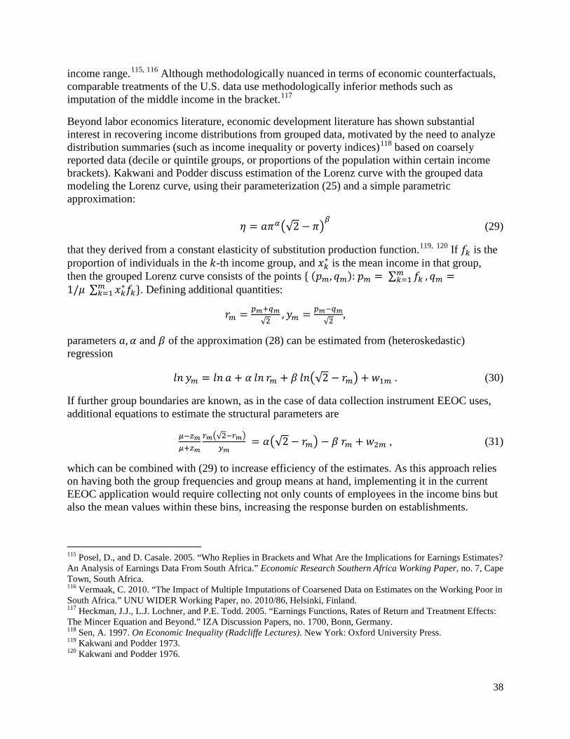
income range.115, 116 Although methodologically nuanced in terms of economic counterfactuals, comparable treatments of the U.S. data use methodologically inferior methods such as imputation of the middle income in the bracket.117

Beyond labor economics literature, economic development literature has shown substantial interest in recovering income distributions from grouped data, motivated by the need to analyze distribution summaries (such as income inequality or poverty indices)118 based on coarsely reported data (decile or quintile groups, or proportions of the population within certain income brackets). Kakwani and Podder discuss estimation of the Lorenz curve with the grouped data modeling the Lorenz curve, using their parameterization (25) and a simple parametric approximation:

𝜂𝜂 = 𝑎𝑎𝜋𝜋𝛼𝛼�√2 − 𝜋𝜋�𝛽𝛽

(29)

that they derived from a constant elasticity of substitution production function.119, 120 If 𝑓𝑓𝑘𝑘 is the proportion of individuals in the 𝑘𝑘-th income group, and 𝑒𝑒𝑘𝑘∗ is the mean income in that group, then the grouped Lorenz curve consists of the points { (𝑒𝑒𝑚𝑚, 𝑞𝑞𝑚𝑚): 𝑒𝑒𝑚𝑚 = ∑ 𝑓𝑓𝑘𝑘𝑚𝑚

𝑘𝑘=1 , 𝑞𝑞𝑚𝑚 =1/𝜇𝜇 ∑ 𝑒𝑒𝑘𝑘∗𝑓𝑓𝑘𝑘}𝑚𝑚

𝑘𝑘=1 . Defining additional quantities:

𝑟𝑟𝑚𝑚 = 𝑝𝑝𝑚𝑚+𝑞𝑞𝑚𝑚√2

,𝑦𝑦𝑚𝑚 = 𝑝𝑝𝑚𝑚−𝑞𝑞𝑚𝑚√2

,

parameters 𝑎𝑎,𝛼𝛼 and 𝛽𝛽 of the approximation (28) can be estimated from (heteroskedastic) regression

𝑙𝑙𝑙𝑙 𝑦𝑦𝑚𝑚 = 𝑙𝑙𝑙𝑙 𝑎𝑎 + 𝛼𝛼 𝑙𝑙𝑙𝑙 𝑟𝑟𝑚𝑚 + 𝛽𝛽 𝑙𝑙𝑙𝑙�√2 − 𝑟𝑟𝑚𝑚� + 𝑃𝑃1𝑚𝑚 . (30)

If further group boundaries are known, as in the case of data collection instrument EEOC uses, additional equations to estimate the structural parameters are

𝜇𝜇−𝑧𝑧𝑚𝑚𝜇𝜇+𝑧𝑧𝑚𝑚

𝑟𝑟𝑚𝑚�√2−𝑟𝑟𝑚𝑚�𝑦𝑦𝑚𝑚

= 𝛼𝛼�√2 − 𝑟𝑟𝑚𝑚� − 𝛽𝛽 𝑟𝑟𝑚𝑚 + 𝑃𝑃2𝑚𝑚 , (31)

which can be combined with (29) to increase efficiency of the estimates. As this approach relies on having both the group frequencies and group means at hand, implementing it in the current EEOC application would require collecting not only counts of employees in the income bins but also the mean values within these bins, increasing the response burden on establishments.

115 Posel, D., and D. Casale. 2005. “Who Replies in Brackets and What Are the Implications for Earnings Estimates? An Analysis of Earnings Data From South Africa.” Economic Research Southern Africa Working Paper, no. 7, Cape Town, South Africa. 116 Vermaak, C. 2010. “The Impact of Multiple Imputations of Coarsened Data on Estimates on the Working Poor in South Africa.” UNU WIDER Working Paper, no. 2010/86, Helsinki, Finland. 117 Heckman, J.J., L.J. Lochner, and P.E. Todd. 2005. “Earnings Functions, Rates of Return and Treatment Effects: The Mincer Equation and Beyond.” IZA Discussion Papers, no. 1700, Bonn, Germany. 118 Sen, A. 1997. On Economic Inequality (Radcliffe Lectures). New York: Oxford University Press. 119 Kakwani and Podder 1973. 120 Kakwani and Podder 1976.

38

Bishop et al. note that estimates of income inequality (and hence, potentially, discrimination in the current application) are highly sensitive to the assumptions made regarding the highest incomes when the latter are top-coded.121 In their analysis, the Pareto distribution with polynomial tails was used to obtain the mean income in the top bracket that does not have the right end point, and leads to revised estimates of income inequality expressed as the Gini coefficient from 0.38 to 0.44 (which, in terms of income distributions in the late 2000s, is the difference between Iceland and Canada; the United States has an even higher level of income inequality, with a Gini index of at least 0.48). They noted, however, that using this model, mean income was only 92 percent of the true mean income obtained from microdata; as a result their model may not be fully adjusting the truncation biases.

To arrive at an estimate of global income inequality, Chotikapanich et al. make a convenient assumption that income is lognormally distributed within a country to create their model of global income distribution.122 When only grouped income data are available, they use a linear interpolation to estimate the Gini index, through which they obtain the lower bound.

Schader and Schmid review the various proposed models based on grouped data, both for parametric representation of the Lorenz curve itself and for the underlying income distributions, when both the proportions and the means within classes are available. They note that “advances in this field of research were fairly erratic.” 123 Using 16 years of data on income distribution in Western Germany covering a 40-year range, they compared 13 parametric approximations to either the underlying income distributions or the Lorenz curve itself. They found that (1) one model produced implausible (non-convex) Lorenz curves; (2) most models produced estimates of the Gini index that were outside of Gastwirth’s nonparametric bounds,124 and some models never produced the values of the Gini index inside these bounds; (3) only three methods produced all estimates within the bounds: Kakwani and Podder’s two-parameter approximation to Lorenz curve,125 Kakwani’s two-parameter beta approximation,126 and Schader and Schmid’s own three-parameter functional form of the curve, which is a generalization of Kakwani’s two parameter functional form.

Hajargasht et al. provided the most general framework of estimating the parameters of the GB2, distribution reviewed in “Parametric Distribution Modeling and Comparison,” and five of its special cases.127 They analytically derived the asymptotic covariance matrix of the group

121 Bishop, J. A., Chiou, J.-R., Formby, J. P., Jan. 1994. Truncation bias and the ordinal evaluation of income inequality. Journal of Business & Economic Statistics 12 (1), 123–127. URL http://dx.doi.org/10.1080/07350015.1994.10509995. 122 Chotikapanich, D., Valenzuela, R., D. S. Prasada Rao, 1998. Global and regional inequality in the distribution of income: Estimation with limited and incomplete data. In: Slottje, D., Raj, B. (Eds.), Income Inequality, Poverty, and Economic Welfare. Studies in Empirical Economics. Physica-Verlag HD, pp. 65-78. URL http://dx.doi.org/10.1007/978-3-642-51073-1_5 123 Schader, M., and F. Schmid. 1994. “Fitting Parametric Lorenz Curves to Grouped Income Distributions – A Critical Note.” Empirical Economics 19(3), 361–370. 124 Gastwirth, J.L. 1972. “The Estimation of the Lorenz Curve and Gini Index.” Review of Economics and Statistics 54, 306–316. 125 Kakwani and Podder 1976. 126 Kakwani, N. 1986. Analyzing Redistribution Policies: A Study Using Australian Data. New York: Cambridge University Press. 127 Hajargasht et al. 2012.

39

proportions and means, making it feasible to use the asymptotically efficient generalized method of moment estimation and obtain goodness of fit tests. Although this work’s generalization was important, it neglected other contributions highlighted in this report, such as Kakwani and Podder;128 Gastwirth, Nayak, and Krieger;129 and Schader and Schmid,130 and thus failed to reveal whether their fully parametric approach did or did not work better than these alternative approaches and nonparametric bounds on inequality coefficients.

Instead of relying on the best-fitting model, von Hippel, Scarpino, and Holas propose using multimodel inference averaging results from different models with weights based on Bayesian information criteria.131 They applied the methodology to the data on 3,221 U.S. counties using the GB2 family of distributions (GB2 root and nine other special cases). They found that fitting the GB2 distribution did not converge 1.0 percent of the time. The estimated parameters implied undefined distribution moments such as means and variance 4.4 percent of the time. The fit of the GB2 model, measured by the likelihood ratio, was rejected 76.0 percent of the time (the authors, however, did not attempt to adjust for multiple testing, as discussed in “Error Rates of Statistical Tests”). Their definition of reliability, taken uncritically from mainstream measurement theory in social sciences, is based on the correlation between their estimate and the true reported value and therefore improperly centers the between-county distribution of the Gini indices, sweeping potential biases under the carpet as a result (as observed by Schader and Schmid, the members of the GB2 family tend to overestimate the value of the Gini index).132 The discrepancies between the model-based and actual values of Gini are due to biases because of model misfit rather than a Gaussian mean zero noise, as assumed in the measurement literature where the concept of reliability is introduced. A better measure of the performance of their estimates would have been the use of Gastwirth bounds on the Gini index, as was done in Schader and Schmid.133, 134

An entirely different approach can be taken to create fully synthetic data sets that are compatible with the reported group data.135 The resulting synthetic data sets can be analyzed using any of the methods that can be used for the individual-level data. Shorrocks and Wan developed an approach to recover the marginal income distribution using the reported summaries by income groups.136 Their two-step algorithm first creates a rough approximation to the underlying distribution using a reasonably close-fitting parametric distribution, such as a lognormal, generalized beta, or Singh-Maddala, and then fine-tuning the income values within each bracket to obtain the match with the reported data. Although it is specifically formulated as a large sample synthetic data simulation approach (they indicate that the method works best with

128 Kakwani and Podder 1976. 129 Gastwirth, J. L., Nayak, T. K., Krieger, A. M., 1986. Large sample theory for the bounds on the Gini and related indices of inequality estimated from grouped data. Journal of Business & Economic Statistics 4 (2), 269-273. 130 Schader and Schmid 1994. 131 von Hippel, P. T., Scarpino, S. V., Holas, I. 2015. Multimodel estimates of inequality from binned incomes. arXiv:1402.4061 [stat.ME], available from http://arxiv.org/abs/1402.4061v5 132 Schader and Schmid 1994. 133 Gastwirth 1972. 134 Schader and Schmid 1994. 135 Drechsler 2011. 136 Shorrocks, A.F., and G. Wan. 2008. “Ungrouping Income Distributions: Synthesizing Samples for Inequality and Poverty Analysis.” UNU-WIDER Working Paper, no. 2008/16, Helsinki, Finland.

40

𝑙𝑙 ≥ 2000), the Shorrocks-Wan approach can plausibly be utilized to create synthetic data sets using the paybands in the separate demographic groups, although it would need to be reformulated as a multiple imputation approach. In passing, Shorrockas and Wan noted that some of the existing approaches to approximate Lorenz curves (including the production code in the World Bank’s POVCAL program) produced implausible negative values when applied to some of the actual income distributions.137

There exists limited literature on the optimal choice of the cutoff points for the groups. Aghevli and Mehran approach the problem by minimizing the difference between the Gini coefficients of the original continuous and the crude grouped data.138 They propose the following rule:

𝑧𝑧𝑘𝑘 = 𝔼𝔼[𝑦𝑦|𝑧𝑧𝑘𝑘−1 ≤ 𝑦𝑦 ≤ 𝑧𝑧𝑘𝑘+1] , (32)

that is, the cutoff point should be the conditional mean of incomes of the two groups it separates. They show that the income grouping using intervals of equal length on income scale is optimal for the uniform distribution of income, and income grouping that allocates equal shares of the total income to each group is optimal for Pareto distribution with shape parameter 2 (with CDF given by 𝐹𝐹(𝑒𝑒) = 1 − (𝑎𝑎/𝑒𝑒)2, 𝑒𝑒 ≥ 𝑎𝑎). They also discuss other potential objective functions for income grouping. Davies and Shorrocks refine their work to point out that the condition (31) is neither necessary nor sufficient for optimal grouping and may not even be feasible with finite population or samples.139 They derive a different condition:

𝑚𝑚𝑎𝑎𝑒𝑒{𝑦𝑦:𝑦𝑦 ≤ 𝑧𝑧𝑘𝑘} ≤ 𝔼𝔼[𝑦𝑦|𝑧𝑧𝑘𝑘−1 ≤ 𝑦𝑦 ≤ 𝑧𝑧𝑘𝑘+1] ≤ 𝑚𝑚𝑖𝑖𝑙𝑙{𝑦𝑦:𝑦𝑦 ≥ 𝑧𝑧𝑘𝑘} , (33)

that is, they provide bounds for 𝑧𝑧𝑘𝑘 rather than exact equality. Davies and Shorrocks provide an algorithm to obtain the groupings and prove that it converges in a finite number of steps.140 They applied their approach to income distribution in Canada and found that in breaking income into 20 groups, their optimal grouping broke down the lower 80 percent of the distribution into groups composed of about 6.5 percent each, and the upper quintile was broken into finer groups, each with about 4 percent of the population, with the top group composed of 1 percent of the top earners. This structure illustrates the importance of accurately tracking income distribution at the very top, which was also noted by other authors (including Bishop et al.).141

Survey Design and Its Impact on the Measures of Dispersion, Degrees of Freedom, and Statistical Power

Survey Design Options Among the survey design options, the following have been considered:

1. Modify the current EEO forms, such as by adding pay bands to the EEO-1 form as in the EEO-4 form. The resulting ordinal pay data would prevent direct use of regression model

137 Shorrocks and Wan 2008. 138 Aghevli, B.B., and F. Mehran. 1981. “Optimal Grouping of Income Distribution Data.” Journal of the American Statistical Association 76(373), 22–26. 139 Davies, J.B., and A.F. Shorrocks. 1989. “Optimal Grouping of Income and Wealth Data.” Journal of Econometrics 42, 97–108. 140 Davies and Shorrocks 1989. 141 Bishop et. al. 1994

41

(1) with microdata, although modifications of the model accounting for the aggregated nature of the data would be feasible.142 (See “Analyses With the Group-Level Data” for a detailed description of this option.)

2. Multiway matching of administrative data, for example, based on existing EEOC forms with other employer-side data and employee-side data, including SSA data on Social Security wages and salaries and Internal Revenue Service (IRS) data from W-2 forms. As is often the case with administrative data, the existing data are collected for purposes other than the analysis of pay discrimination. The definitions of wages and salaries for SSA or IRS purposes may not match the definitions that are appropriate for the analysis of pay discrimination. In particular, because SSA and IRS collect only the annual totals, pay rates may not be determined from these data unless additional data on hours worked are collected for each employee.

3. One of the possibilities that was discussed involved collecting the range of pay along with the average pay and using techniques such as those proposed by Hozo et al.143 We cannot consider their approach as viable because it produces biased estimates for the typical right-skewed populations encountered in the analysis of pay data and therefore inappropriate for important policy applications.

Other components of the design that may have implications for the analysis relate to industry and geographic classification. The primary industry classification system used in the United States is the North American Industry Classification System (NAICS), which uses a six-digit hierarchical coding system to classify all economic activity into 20 industry sectors. Five sectors are mainly goods-producing sectors and 15 are entirely services-producing sectors.144 NAICS allows for the identification of 1,170 industries. Beyond the top two-digit level identifying the 20 primary sectors, there are 99 sectors defined by 3 digits, 312 sectors defined by 4 digits, 716 sectors defined by 5 digits, and 1065 sectors defined by 6 digits. The levels of geography likewise have a multilevel hierarchical structure. The U.S. Census Bureau divides the nation into 4 regions, 9 divisions, 50 states, and 3,141 counties or statistically equivalent entities within states. The U.S. Census Bureau also defines ZIP code tabulation areas (ZCTAs) that are closely related to the U.S. Postal Service’s five-digit ZIP code service areas; ZCTAs may cross county and even state lines. Independently of states, the U.S. Census Bureau also defines urban areas, 250 metropolitan areas (a city or an urban area of at least 50,000 inhabitants with a total population of at least 75,000 in New England or 100,000 everywhere else), micro areas (areas with an urban core of at least 10,000 but less than 50,000), and other types of geographies. Bureau of Labor Statistics defines 4,742 labor market areas based on metropolitan, micropolitan and small labor market areas, and commuting patterns. The appropriate location definitions should be chosen to ensure that establishments that are compared in the same location correspond to the same labor market.

Because Section I of this report proposes the use of W-2 data arranged in pay bands, investigators must consider whether individuals within a demographic group and a pay band are really comparable. In particular, individuals with different pay rates may end up in the same bin

142 Long 1997. 143 Hozo et al. 2005. 144 Office of Management and Budget. 2012. North American Industry Classification System: 2012 NAICS Definitions. Available at http://www.census.gov/eos/www/naics/2012NAICS/2012_Definition_File.pdf.

42

if they worked a different number of hours, such as when a more highly paid individual joined or left the company in midyear. To account for these circumstances, the new EEOC form will record the total hours worked. The log of total hours can be used in Mincer wage equation (1) with a fixed coefficient of 1 (often referred to as offset in biometric literature, where such offsets are used in Poisson regression for counts of adverse events to correct for the different exposures to the risk factors by different individuals). If an individual performed work at rates that are higher than the regular rates (such as for overtime work), these hours may have to be accounted at these higher rates to ensure comparability of pay rates.

Measures of Dispersion In most tests discussed above, measures of dispersion play a crucial role in obtaining the test statistics. The sample variances figure explicitly in t-tests (4) and (7), and the estimate of the residual variance 𝜎𝜎2 appears in the denominator of the F-test associated with Mincer wage equation (1). The available measures of dispersion will depend on the survey design. With detailed individual-level pay data, such as that obtained from the matched IRS Form W-2 data, any relevant measure can be computed. With the aggregated group-level data, the measures of dispersion will have to be either collected explicitly (for example, by augmenting the EEO-1 form to include the mean and the standard deviation of pay levels in addition to the number of employees in a given job category by race/ethnicity and gender cells) or estimated from other data (such as pay band data; see “Analyses With the Group-Level Data” on the use of interval regression for this statistical task).

Degrees of Freedom The number of degrees of freedom is the number of values in the calculation of statistics that are allowed to vary freely; that is, the number of ways in which the final result can be modified by changing the inputs. In many statistical problems, the number of degrees of freedom is given by the number of observations in the sample 𝑙𝑙, and this number is reduced for each parameter that is estimated. For linear problems, such as estimation of a group mean or a regression coefficient, one degree of freedom is taken out for each estimated parameter.

Many distributions used as the reference distributions for statistical tests are characterized by degrees of freedom as one of their parameters. For instance, the chi-square distribution with 𝑘𝑘 degrees of freedom is the distribution of the sum of squares of 𝑘𝑘 independent standard normal variates. Related to the chi-square are Student’s t-distribution, which is the ratio of a standard normal variate to a chi-square with 𝑘𝑘 degrees of freedom independent from it, and Fisher’s F-distribution, commonly arising in linear models, which is the ratio of two independent chi-squares or, in the context of linear models, including ANOVA, the variance of the outcome explained by the model to the residual variance.145 These distributions typically are used to produce critical values for frequentist tests or to form confidence intervals around parameter estimates. As lower degrees of freedom are usually associated with smaller sample sizes, t and 𝐹𝐹 distributions with low degrees of freedom demonstrate heavy-tailed behaviors, allowing for greater uncertainties associated with smaller sample sizes.

A common rule of thumb is that the number of degrees of freedom is equal to the number of observations minus the number of estimated parameters. This rule, however, does not work in

145 Rao 2001.

43

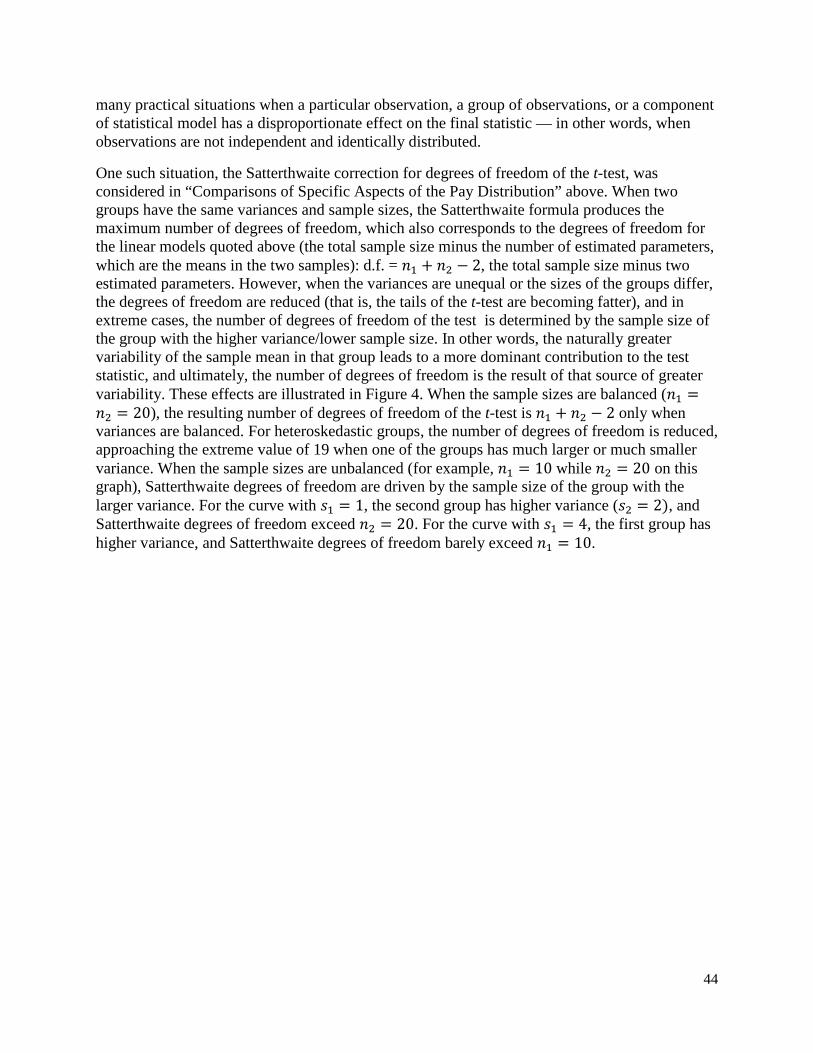
many practical situations when a particular observation, a group of observations, or a component of statistical model has a disproportionate effect on the final statistic — in other words, when observations are not independent and identically distributed.

One such situation, the Satterthwaite correction for degrees of freedom of the t-test, was considered in “Comparisons of Specific Aspects of the Pay Distribution” above. When two groups have the same variances and sample sizes, the Satterthwaite formula produces the maximum number of degrees of freedom, which also corresponds to the degrees of freedom for the linear models quoted above (the total sample size minus the number of estimated parameters, which are the means in the two samples): d.f. = 𝑙𝑙1 + 𝑙𝑙2 − 2, the total sample size minus two estimated parameters. However, when the variances are unequal or the sizes of the groups differ, the degrees of freedom are reduced (that is, the tails of the t-test are becoming fatter), and in extreme cases, the number of degrees of freedom of the test is determined by the sample size of the group with the higher variance/lower sample size. In other words, the naturally greater variability of the sample mean in that group leads to a more dominant contribution to the test statistic, and ultimately, the number of degrees of freedom is the result of that source of greater variability. These effects are illustrated in Figure 4. When the sample sizes are balanced (𝑙𝑙1 =𝑙𝑙2 = 20), the resulting number of degrees of freedom of the t-test is 𝑙𝑙1 + 𝑙𝑙2 − 2 only when variances are balanced. For heteroskedastic groups, the number of degrees of freedom is reduced, approaching the extreme value of 19 when one of the groups has much larger or much smaller variance. When the sample sizes are unbalanced (for example, 𝑙𝑙1 = 10 while 𝑙𝑙2 = 20 on this graph), Satterthwaite degrees of freedom are driven by the sample size of the group with the larger variance. For the curve with 𝑠𝑠1 = 1, the second group has higher variance (𝑠𝑠2 = 2), and Satterthwaite degrees of freedom exceed 𝑙𝑙2 = 20. For the curve with 𝑠𝑠1 = 4, the first group has higher variance, and Satterthwaite degrees of freedom barely exceed 𝑙𝑙1 = 10.

44

Figure 4. Satterthwaite degrees of freedom for Welch t-test. ( function ((s11^2/x) + (s2^2/n2))^2 / ( s11^4/(x*x*(x-1)) + s2^4/(n2*n2*(n2-1) 1 "s{subscript:1}=1" ) label( 2 "s{subscript:1}=2" ) label(3 "s{subscript:1}=4") label( 4 "d.f. =

Another situation of reduced degrees of freedom arises in complex survey sampling designs. When the sample is taken in a multistage design, producing a clustered sample, the degrees of freedom are commonly computed as the number of primary sampling units (because in cases in which all observations within a primary sampling unit are identical, it contributes only one degree of freedom along which the results can vary) minus the number of strata (because strata means are estimated when computing sampling variances). In this case, a group of observations, a primary sampling unit, contributes less to the ultimate degrees of freedom than the full number of observations in that group. When the sample has unequal weights because of differing sampling and response probabilities, observations with greater weights have greater effect on the final statistics than observations with smaller weights, and the final result varies less in response to these lower-weight observations. Unequal weighting therefore has effect on both the sample size, resulting in an effective sample size that is typically smaller than the nominal sample size

𝑙𝑙� = �∑ 𝑤𝑤𝑊𝑊𝑙𝑙𝑊𝑊=1 �2

∑ 𝑤𝑤𝑊𝑊2𝑙𝑙

𝑊𝑊=1, (34)

as well as on the degrees of freedom for variance estimation.146 Potthoff et al. propose alternative expressions for the degrees of freedom of unequally weighted complex survey data that depend on the third and the fourth moments of weights:

146 Korn, E. K., and B. I. Graubard. 1999. Analysis of Health Surveys. New York: Wiley & Sons, pp. 172–176.

020

4060

80S

atte

rthw

aite

d.f.

0 10 20 30 40 50n1

s1=1 s1=2s1=4 d.f. = n1+n2-2

s2=2, n2=20

45

𝑑𝑑.𝑓𝑓. = 2(𝑙𝑙�−1)2

𝐵𝐵, 𝐵𝐵 = 2 + (𝜅𝜅 − 1)𝑙𝑙� − 2

𝑙𝑙�(𝜅𝜅 − 1)∑ 𝑃𝑃𝑖𝑖

3𝑙𝑙𝑖𝑖=1 + 1

𝑙𝑙�2(𝜅𝜅 − 3)∑ 𝑃𝑃𝑖𝑖

4𝑙𝑙𝑖𝑖=1 , 𝜅𝜅 = 𝔼𝔼[ (𝑦𝑦𝑊𝑊−𝜇𝜇)4]

𝑦𝑦4. 147(35)

Valliant and Rust consider a stratified sample with unequal strata variances 𝜎𝜎ℎ2 and sample sizes 𝑙𝑙ℎ in stratum ℎ = 1, … , 𝐿𝐿, and arrive at an expression for degrees of freedom that involves higher order moments of data:

𝑑𝑑.𝑓𝑓. =2�∑

𝜎𝜎ℎ2

𝑙𝑙ℎ𝑙𝑙ℎ=1 �

2

∑𝜎𝜎ℎ4

𝑙𝑙ℎ3

𝑙𝑙ℎ=1 �𝜅𝜅ℎ−

𝑙𝑙ℎ−3𝑙𝑙ℎ−1

� .148 (36)

The cumulative effect of all features of complex survey designs is accommodated in the degrees of freedom of statistical tests and information criteria via the generalized design effects.149, 150

Finally, in flexible models such as those arising in machine learning, more than one degree of freedom may need to be removed — for example, in regression trees, one node corresponds to about three degrees of freedom.151

The issue of degrees of freedom can become even more complicated when analyzing aggregated data, such as in pay bands by target group. While the number of people in a given cell can be used in computing the Satterthwaite degrees of freedom (5) for a two-sample t-test, the use of the cell values in other analyses, such as regression models, may produce as little as one degree of freedom per cell, so that the overall sample size is the number of cells rather than the number of individuals in these cells.

Error Rates of Statistical Tests Statistical testing procedures are usually characterized by two error rates:

1. Type I error rate (denoted as 𝛼𝛼), or significance level, characterizes the probability of a false alarm when the test concludes that there is evidence against the null hypothesis even though the null hypothesis is actually true. When the null is that of no discrimination, such as posited in hypotheses (2) or (3), a type I error occurs when a flag is raised against a company that does not discriminate against its employees, with the test producing a significant result simply by chance. Significance level is then the proportion of investigations that will end up not finding any evidence of discrimination. This parameter therefore characterizes the operational efficiency of the EEOC statistical procedures.

147 Potthoff, R. F., M.A. Woodbury, and K.G. Manton. 1992. “‘Equivalent Sample Size’ and ‘Equivalent Degrees of Freedom’ Refinements for Inference Using Survey Weights Under Superpopulation Models.” Journal of the American Statistical Association 87(418), 383–396. 148 Valliant, R., and K.F. Rust. 2010. “Degrees of Freedom Approximations and Rules-of-Thumb.” Journal of Official Statistics 26(4), 585–602. 149 Rao, J.N.K., and D.R. Thomas. 2003. “Analysis of Categorical Response Data From Complex Surveys: An Appraisal and Update.” In: Chambers, R.L., and C.J. Skinner Analysis of Survey Data. New York: Wiley, 85–108. 150 Lumley, T., and A. Scott. 2015. “AIC and BIC for Modeling With Complex Survey Data.” Journal of Survey Statistics and Methodology, in press. 151 Ye, J. 1998. “On Measuring and Correcting the Effects of Data Mining and Model Selection.” Journal of the American Statistical Association 93(441), 120–131.

46

2. Type II error rate (denoted as 𝛽𝛽, not to be confused with the symbol used to denote regression coefficients) is an error of omission rate, in which the test concludes that there is not enough evidence against the null hypothesis even though the alternative hypothesis is true. When the null is that of no discrimination, a type II error is that of missing an establishment because its discriminatory practices do not manifest strongly enough. This parameter thus characterizes equitability of the EEOC statistical procedures.

The complement of the type II error rate, 1 − 𝛽𝛽, is referred to as power of the test. The type I error rate is also called the significance level, or the size of the test. The most common values used in statistical practice are values of 1%, 5%, and 10% for 𝛼𝛼, and 80% for power.

Some tests, such as the t-test or the Wilcoxon-Mann-Whitney test, can be made directional, or one-sided. That is, the statistical test can be formulated to be sensitive to differences only when the mean pay of the protected group is lower than the mean pay of the majority group. Considerations for the use of one-sided tests in establishing discrimination usually involve the known history of discrimination that manifests in lower pay. A two-sided statistical test, on the other hand, is the one that is sensitive to either positive or negative differences between the two groups. Both the t-test and Wilcoxon-Mann-Whitney test can be formulated as either one-sided or two-sided tests. Other tests, such as Kolmogorov-Smirnov test or tests that rely on squared quantities (and have 𝜒𝜒2 or 𝐹𝐹-distributions, such as those arising in analysis of contingency tables or in regression models with multiple coefficients being tested simultaneously), are inherently two-sided. The one-sided tests have greater power when the alternative is in the hypothesized direction but have no power when the alternative is in the opposite direction (that is, when the protected group earns more than the reference group). Good notes that the use of one-tail vs. two-tail tests often causes confusion and argues in favor of one-sided tests when the direction of the socially undesirable outcome that the court needs to guard against is clear.152 He cites the toxicity of a chemical compound as an example, in which basic biology implies that an increase in a dose leads to higher cancer rates, thus justifying the use of one-sided test.

When different tests for the same null hypotheses are available, one can compare the tests that have the same size (the probability of a false alarm or type I error). For example, Durbin derives the power of Kolmogorov-Smirnov test and, in one of the applications of the theoretical result, compares its power with that of the power of the “optimal” test for an exponential distribution based on the sample mean.153 He found that the asymptotic power of Kolmogorov-Smirnov test was lower (about 81% asymptotic power against a sequence of local alternatives where the optimal test is calibrated to have 95% power), and the small sample power of Kolmogorov-Smirnov test was worse still. However, the primary strength of a nonparametric test such as the Kolmogorov-Smirnov test is that it does not depend on whether the researcher has correctly identified the parametric distribution, such as the normal distribution, as required by parametric tests that assume a specific distribution.

152 Good 2001, pp. 150–152. 153 Durbin, J. 1971. “Boundary-Crossing Probabilities for the Brownian Motion and Poisson Processes and Techniques for Computing the Power of the Kolmogorov-Smirnov Test.” Journal of Applied Probability 8(3), 431–453.

47

In most statistical applications, the issue of power arises at the planning stages of a study when determining the sample size to be collected.154 In the current application, because the EEOC data are collected for all full-time employees of all eligible establishments, the sample size is fixed in advance and is equal to the number of establishments in the industry or industry-location cells for analysis of the industry as a whole, and to the number of eligible employees of the establishment for the analysis and investigation of an establishment. In addition, EEOC’s routine practices lead to the issue of multiple testing (that is, the same hypothesis is applied to a number of establishments), which can create problems with controlling the overall size of the test.155

As a simple example, consider conducting 𝐾𝐾 = 100 independent tests at the 5% significance level. When the null hypothesis is true, about 5 tests would come out significant at 5% level (strictly speaking, the number of significant tests will follow a binomial distribution with n=100 and p=0.05 that has a mean of 5). If the alternative is that in at least one of the 100 tests, the null hypothesis is wrong, and the rejection rule is to reject when at least one test is significant at level 𝛼𝛼0, then the overall probability of rejection is 𝛼𝛼 = 1 − (1 − 𝛼𝛼0)𝐾𝐾. If this is to be set to 5%, then the individual rejection level is to be set to 𝛼𝛼0 = 1 − √1 − 𝛼𝛼𝐾𝐾 = 1 − 0.051/100 = 0.000513, much lower than the original value of 5%. A similar value is given by a conservative bound known as the Bonferroni correction, 𝛼𝛼𝐵𝐵 = 𝛼𝛼/𝐾𝐾 = 0.0005. More accurate testing procedures aimed at controlling false discovery rates have been used during the past 20 years in areas such as genomics, where the statistical tasks are often formulated for microarrays that may register tens of thousands genes, leading to the corresponding number of hypothesis being tested (e.g., whether a given gene affects a disease).156 The Benjamini-Hochberg-Yekutieli false discovery rate procedure identifies the hypotheses that should be rejected as follows:

1. Sort the 𝑒𝑒-values of individual hypotheses in an ascending order: 𝑃𝑃(1),≤ 𝑃𝑃(2) ≤ ⋯ ≤𝑃𝑃(𝐾𝐾).

2. For a given 𝛼𝛼, find the largest 𝑘𝑘 such that 𝑃𝑃(𝑘𝑘) ≤𝑘𝑘𝛼𝛼

𝑚𝑚𝑐𝑐(𝑚𝑚) , 𝑐𝑐(𝑚𝑚) = ∑ 𝑙𝑙−1𝑚𝑚𝑙𝑙=1 ≈ ln𝑚𝑚 +

𝛾𝛾 = ln𝑙𝑙 + 0.5772. 3. Reject all the null hypotheses 𝐻𝐻(1),𝐻𝐻(2), … ,𝐻𝐻(𝑚𝑚) corresponding to the 𝑒𝑒-values

𝑃𝑃(1),𝑃𝑃(2), … ,𝑃𝑃(𝑚𝑚).

This procedure provides justification for the descriptive ranking approach outlined earlier, where we suggested listing the companies that seem to deviate most from the null hypothesis (or the values typical for the industry), and provides the cutoff for the establishments that need to be investigated.

Good calls for the government regulations to “be drafted so as to specify either the sample size and cut-off criteria or acceptable values of Type I and Type II errors.”157 In the context of the current application, one can argue that the EEOC may want to consider setting the parameters of

154 Ryan, T.P. 2013. Sample Size Determination and Power. Hoboken, New Jersey: Wiley. 155 Dmitrienko, A., A.C. Tamhane, and F. Bretz (eds.). 2009. Multiple Testing Problems in Pharmaceutical Statistics. Chapman & Hall/CRC Biostatistics Series. Boca Raton, Florida: Chapman and Hall/CRC. 156 Benjamini, Y., and Y. Hochberg. 1995. “Controlling the False Discovery Rate: A Practical and Powerful Approach to Multiple Testing.” Journal of the Royal Statistical Society, Series B (Methodological) 57(1), 289–300. 157 Good 2001, 129.

48

statistical tests to optimize their performance.158 Within the framework of statistical decision theory, one needs to define the loss function associated with the costs of different errors.

The cost of type I errors to society includes (1) the cost of EEOC to investigate the case, plus, potentially, (2) the cost for the establishment to respond to the discrimination claim, plus, potentially, (3) the cost to cover court fees if the charges are brought to court but no evidence of discrimination is found (recall that type I errors occur under the null hypothesis of no discrimination).

The cost of type II errors includes (1) the lost income of the employees who have been discriminated against, as well as (2) the reputation costs of discrimination to society at large. If these costs can be quantified, EEOC can optimize the decision rules by choosing the significance level, or action threshold, over which an investigation is to be triggered. If this threshold is set too low (on a scale where large values are associated with stronger evidence of discrimination), too many establishments will be investigated, including many that do not discriminate, wasting EEOC resources. If this threshold is set too high, then some companies that engage in discrimination may fall below the radar and avoid being investigated.

Without quantifying these costs, it is difficult to provide further advice regarding the error rates that EEOC should be targeting in its investigations. The frequently used figures of 5% or 1% significance (false alarm rates; establishments investigated where no discrimination exists) and 80% power (probability of finding discrimination in an organization that truly discriminates) are guided by considerations entirely different than those EEOC is facing. In particular, if EEOC adopts the framework of optimizing the error rates based on the costs of incorrect decisions, a sliding scale will be created in which the optimal rates depend on the establishment size: while the cost of investigation varies slowly over establishments of different sizes, the societal costs are increasing proportionally to the establishment size, assuming that a constant fraction of the employees are experiencing discriminated. Thus with higher societal costs in larger establishments, the action threshold should be lowered for larger establishments.

Suppose an EEOC investigator is investigating a company with 80 employees, of whom 50% are women, and average earnings are $20,000. If the female employees are discriminated so that their pay rate is 10% lower than that of males, the annual societal cost of discrimination is 𝐶𝐶𝑆𝑆 = 80 employees × 50% female × $20,000 average × 10% disparity = $80,000. Suppose the cost (to the EEOC) of investigation is 20 hours of investigator’s time = $2,000=𝐶𝐶𝐼𝐼. Using the traditional statistical notation for the Type I error rate as 𝛼𝛼 and type II error as 𝛽𝛽, the total expected cost is the sum of the cost for each outcome times its probability: 𝐶𝐶𝐸𝐸 = 𝛼𝛼𝐶𝐶𝐼𝐼 + 𝛽𝛽𝐶𝐶𝑆𝑆. If the (asymptotic) distributions of the test statistic 𝑇𝑇 under both the null and the alternative are normal159 𝑁𝑁(𝜇𝜇0,𝜎𝜎2) and 𝑁𝑁(𝜇𝜇1,𝜎𝜎2), respectively, then the one-sided critical value for a rejection region 𝑇𝑇 > 𝑇𝑇0 is given by 𝑇𝑇𝑐𝑐 = 𝜇𝜇0 + 𝜎𝜎𝑧𝑧𝛼𝛼, and the probability of type II error of inclusion is Prob[𝑇𝑇 < 𝑇𝑇𝑐𝑐] = Φ(𝜇𝜇0−𝜇𝜇1

𝑦𝑦+ 𝑧𝑧𝛼𝛼), where the 𝛼𝛼-level upper percentile is 𝑧𝑧𝛼𝛼 = Φ−1(1 − 𝛼𝛼), and Φ(𝑧𝑧) is the

standard normal cdf. Thus the final expression for the expected cost is

158 DeGroot, M. H. 2004. Optimal Statistical Decisions. New York: Wiley-Interscience. 159 Noether 1987.

49

𝐶𝐶𝐸𝐸(𝛼𝛼) = 𝛼𝛼𝐶𝐶𝐼𝐼 + 𝛷𝛷 �𝜇𝜇0−𝜇𝜇1𝑦𝑦

+ 𝛷𝛷−1(1− 𝛼𝛼)� 𝐶𝐶𝑆𝑆 (37)

Differentiating with respect to α and setting the derivative to zero, we can find the optimal enforcement level α as the solution to:

0 = 𝑑𝑑 𝐶𝐶𝐸𝐸𝑑𝑑𝛼𝛼

= 𝐶𝐶𝐼𝐼 + 𝜑𝜑 �𝜇𝜇0−𝜇𝜇1𝑦𝑦

+ 𝑧𝑧𝛼𝛼� �−1

𝜑𝜑(𝑧𝑧𝛼𝛼)� 𝐶𝐶𝑆𝑆;

𝐶𝐶𝐼𝐼𝐶𝐶𝑆𝑆� =

𝜑𝜑 �𝜇𝜇0−𝜇𝜇1𝑦𝑦

+ 𝑧𝑧𝛼𝛼�𝜑𝜑(𝑧𝑧𝛼𝛼)� .

The asymptotic distribution of Mann-Whitney-Wilcoxon test is 𝑁𝑁(𝑙𝑙1𝑙𝑙2𝑒𝑒′,𝑙𝑙1𝑙𝑙2(𝑙𝑙1 + 𝑙𝑙2 +1)/12) where 𝑒𝑒′ is the probability that an observation from one group (male earnings) is greater than an observation from the other group (female earnings); 𝑒𝑒′ = 0.5 under the null of no discrimination. Using the “middle income” scenario results from section “Power analysis with grouped data” below, we find that 𝑒𝑒′ = 0.609 for MWW test under the alternative using the optimal grouping of incomes proposed in that section. For the selected company size, 𝑙𝑙1 = 𝑙𝑙2 =40. Thus we need to solve for 𝑧𝑧𝛼𝛼 from equation

0.025 = $2,000$80,000� = 𝜑𝜑(1.678 + 𝑧𝑧𝛼𝛼)

𝜑𝜑(𝑧𝑧𝛼𝛼)�

Figure 5. Numeric solution for the optimization of error rates.

0.0

5.1

.15

.2.2

5R

atio

of n

orm

al d

ensi

ties

0 .1 .2 .3 .4 .5Type I error

50

Solution to this equation (see Figure 5) is given by 𝑧𝑧𝛼𝛼 = 1.36, which corresponds to the optimal type I error rate (significance) level of 𝛼𝛼 = 8.7%. This is a somewhat more lax criterion than the traditionally used 5% level. For the given company size and gender ratio of the employee pool, the increase in the ratio of the EEOC investigation cost to the societal cost of discrimination is going to lead to an increase in the optimal error rate. An increase in the company size will likely lead to a proportional increase of the societal cost, a disproportionately smaller increase in the investigation costs, and an increase of the noncentrality parameter (𝜇𝜇0 − 𝜇𝜇1)/𝜎𝜎. A more unequal gender ratio will decrease the noncentrality parameter, reducing the power of the test, increasing the type I error rate, and eventually shifting the curve down.

Sparse Cells and Unbalanced Groups

Sample Sizes For most establishments, counts of the number of employees in some, if not most, demographic cells will likely be anywhere from single digits to the low double digits, especially for minorities who are of primary interest. The resulting summaries of pay, such as means, medians, or standard deviations, are inevitably going to be imprecise, which may prevent EEOC from acting on these small companies. Good160 summarizes several dozen court cases focusing on how various courts perceived the sample size issues. In most reported cases, sample sizes below 10 usually were found inadequate to serve as evidence. He finds that the courts use sensitivity analysis (the leave-out-one-or-two rule: the results should not be sensitive to removing or reclassifying one or two persons) and statistical significance as criteria for their decisions. Gastwirth notes that although courts may leave specific significance levels unspecified, a difference of two or three standard deviations, in cases concerning the observed versus expected counts, is likely to provide the data support for a prima facie case of discrimination.161 Two standard deviations correspond to a two-sided significance level of 0.05 and a one-sided significance level of 0.025; three standard deviations correspond to a two-sided significance level of 0.0026 and a one-sided significance level of 0.0013.

The above issues of precision can be viewed as the issue of balancing the error rates as discussed in “Error Rates of Statistical Tests” above. For a fixed level of significance, analysis for smaller establishments will be more likely to miss true discrimination; if the power of tests is fixed, the significance level has to be higher for small establishments — that is, the procedure will generate more false positives. Besides the issue of higher error rates inevitable in smaller samples, there is also the issue of approximations of the test statistics when tests rely on asymptotic arguments. For all of the nonparametric tests we have considered (Wilcoxon-Mann-Whitney, Kruskal-Wallis, Kolmogorov-Smirnov), exact distributions in finite samples are available. Distributions of the two-sample t-tests are based on a normality assumption, and both the Satterthwaite approximate degrees of freedom and Cressie-Whitford corrections for skewness are approximations for the true distributions based on matching several lower order distribution moments. Besides the sample sizes, these distributions have the ancillary parameters of the underlying population variances and, for any sample size, depend on the ratio of these variances, with greater ratios producing worse approximations. Finally, regression-type procedures such as the quantile regression and the interval regression are based on solving estimating equations and

160 Good 2001, pp. 115–129. 161 Gastwirth 2000.

51

have only an asymptotic justification. The degree to which the estimates agree with the asymptotic normal distribution is a complicated function of the sample size and nonlinearity in these estimating equations. Higher-order asymptotic arguments or simulations can provide better insight into the accuracy of inferential decisions based on the use of asymptotic distributions in these models.

Degrees of Freedom in Unbalanced Groups As a more subtle effect, the lower degrees of freedom for smaller samples also lead to wider confidence intervals because of the heavier tails of the t-, 𝜒𝜒2 or 𝐹𝐹-distributions. As demonstrated by the t-test degrees of freedom expression (5) and the discussion that followed there and in “Degrees of Freedom” above, unbalanced groups with small sample sizes pose statistical challenges, resulting in reduced degrees of freedom and, as a result, wider confidence intervals and lower power of statistical tests. Statistical properties of the estimates and tests are often determined by the sample size of the smallest group(s), and for some racial and ethnic minority groups, the counts in small establishments may be in the single digits, and some cells will be empty.

Improving Estimates’ Accuracy by Borrowing Strength Across Industries and Locations One potential way to improve the statistical quality of the estimates is by “borrowing strength” from other, similar units, such as establishments in the same industry or location. In statistics, the approach is best known as small area estimation.162 Small area estimation is an area of active growth and research in survey statistics that emerged in the 1990s following the greater availability of computing power. It concerns the problem of obtaining reasonable estimates for domains where small sample sizes do not allow direct estimation using only survey data (including domains with zero sample observations), such as at the level of a county or a metropolitan area. Because typical national surveys contain at most several dozen observations at these levels, models have been developed to support inference by borrowing strength from the whole data set. A number of large federal statistics programs rely on small area estimates. For example, in 1989 the U.S. Census Bureau launched Small Area Income and Poverty Estimates (SAIPE) for school districts, counties, and states, which have been updated annually since 1995.163 SAIPE data are being used for Title I allocations. The National Cancer Institute runs Small Area Estimates for Cancer Risk Factors and Screening Behaviors to produce estimates of smoking and mammography at the health service-area level.164 The National Center for Health Statistics produces small area estimates for a range of health outcomes.165 Small area estimation approaches are used not only in surveys of individuals but also in establishment surveys.166

162 Rao, J.N.K. 2003. Small Area Estimation. New York: Wiley. 163 National Research Council. 2000. Small-Area Income and Poverty Estimates: Priorities for 2000 and Beyond. Washington, DC: The National Academies Press. 164Raghunathan, T. E., D. Xie, N. Schenker, V. L. Parsons, W. W. Davis, K. W. Dodd, and E. J. Feuer. 2007. Combining information from two surveys to estimate County-Level prevalence rates of cancer risk factors and screening. Journal of the American Statistical Association 102 (478), 474-486. 165 Blumberg, S.J., N. Ganesh, J.V. Luke, and G. Gonzales. 2013. “Wireless Substitution: State-Level Estimates From the National Health Interview Survey, 2012.” National Health Statistics Report 70, National Center for Health Statistics. 166 Hidiroglou, M.A., and P. Smith. 2005. “Developing Small Area Estimates for Business Surveys at the ONS.” Statistics in Transition 7(3), 527–539.

52

The modern approach to small area estimation involves the use of statistical models to predict the variable of interest (such as the proportion of population with a rare characteristic, or measures of central tendency of a continuous variable such as income), typically proceeding in the following steps:

1. An appropriate regression model (linear for continuous response, logistic for binary response, Poisson for counts, etc.) is first formulated for the response of interest. It would use variables available for all sampled areas and all sampled units.

2. This model is fitted to the existing survey data, with sampling weights if available and necessary.

3. Predictions from the model (called synthetic estimators) are obtained. 4. If the area-level data are available from the survey data, direct survey estimators

(weighted means, rates, proportions) are calculated, along with their estimated variances. 5. The synthetic estimators are combined with the direct estimators to minimize the mean

squared error of the resulting composite estimator.

The statistical models underlying small area estimates are typically variations of models called mixed models in biostatistics167 as well as hierarchical or multilevel models in social sciences.168, 169 In a typical two-level model, the regression equation includes not only a random term for the “individual” but also random terms for the “areas,” or the units in which the individuals are nested (such as establishments):

𝑦𝑦𝑖𝑖𝑗𝑗 = 𝑒𝑒𝑖𝑖𝑗𝑗′ 𝛽𝛽 + 𝑢𝑢𝑖𝑖 + 𝜖𝜖𝑖𝑖𝑗𝑗 , (38)

where index 𝑖𝑖 enumerates “areas” and index 𝑗𝑗 enumerates observation units within the areas. Assuming normality of the error terms 𝑢𝑢𝑖𝑖 and 𝜖𝜖𝑖𝑖𝑗𝑗, likelihood for the model as a whole can be derived and maximized to give parameter estimates. Model (17) allows the analyst to answer a variety of questions, including both the standard questions of the traditional regression analysis, such as the impact of covariates 𝑒𝑒𝑖𝑖𝑗𝑗, as well as questions regarding the variability of the outcome due to areas (variance 𝜎𝜎𝑢𝑢2 of the area-specific terms 𝑢𝑢). Predictions of the area effects that “borrow strength” across similar units, referred to as empirical Bayes predictions, are given by

𝑢𝑢�𝑖𝑖𝐸𝐸𝐵𝐵 = 𝛾𝛾𝑖𝑖1𝑙𝑙𝑊𝑊∑ (𝑦𝑦𝑖𝑖𝑗𝑗 − 𝑒𝑒𝑖𝑖𝑗𝑗′ �̂�𝛽)𝑙𝑙𝑊𝑊𝑗𝑗=1 ; 𝛾𝛾𝑖𝑖 = 𝑦𝑦�𝑢𝑢2

𝑦𝑦�𝑢𝑢2+𝜎𝜎�𝜖𝜖2

𝑙𝑙𝑊𝑊

; 𝕍𝕍[𝑢𝑢�𝑖𝑖𝐸𝐸𝐵𝐵] = (1 − 𝛾𝛾𝑖𝑖)𝜎𝜎�𝑢𝑢2 . (39)

The final composite estimates of the area means are given by

𝜇𝜇�𝑖𝑖 = 𝑋𝑋𝑖𝑖⋅′ �̂�𝛽 + 𝑢𝑢�𝑖𝑖𝐸𝐸𝐵𝐵; 𝕍𝕍[𝑦𝑦�𝑖𝑖⋅] = 𝕍𝕍[𝑢𝑢�𝑖𝑖𝐸𝐸𝐵𝐵] + 𝑋𝑋𝑖𝑖⋅′ 𝕍𝕍��̂�𝛽�𝑋𝑋𝑖𝑖⋅ . (40)

This is a simplified expression for the census situation typical for the current application. Full expressions for the small area estimates when the units 𝑗𝑗 are sampled within area 𝑖𝑖 are given in

167 Demidenko, E. 2013. Mixed Models: Theory and Applications with R, 2nd edition. Hoboken, New Jersey: Wiley. 168 Raudenbush, S.W., and A.S. Bryk. 2002. Hierarchical Linear Models, 2nd edition. Thousand Oaks, California: SAGE Publications. 169 Hox, J. 2010. Multilevel Analysis: Techniques and Applications, 2nd edition. New York: Routledge.

53

Rao.170 The second term in the variance expression in (19) is the textbook variance of the prediction error from a linear regression model. From expression (18) for empirical Bayes prediction and its variance, it can be seen how the multilevel model improves the quality of the estimates by trading off the sources of information with different precision. Part of the reduction comes from the explanatory power of the model, so that 𝜎𝜎𝜖𝜖2 + 𝜎𝜎𝑢𝑢2 < 𝜎𝜎𝑦𝑦2 . The variance is reduced to the extent that the model drives the error variances 𝜎𝜎𝑢𝑢2 and 𝜎𝜎𝜖𝜖2 down. Also, empirical Bayes estimates of the area effects are being shrunk toward zero so that the area estimates of the outcome are shrunk toward the model-implied mean, with shrinkage multipliers producing additional variance reduction. Although this effect is generally desirable for estimates that are otherwise imprecise, shrinkage towards the mean may be undesirable for the EEOC applications; it effectively implies that the company behaves like others in the reference group in terms of wage setting, whereas the analysis task at hand is to determine whether the company actually differs from others (assumed compliant with the nondiscrimination requirements). Nevertheless, if shrinkage affects companies of similar sizes in a similar way, their ordering in terms of deviations from the appropriately set wages will likely be retained, still providing valuable information to the EEOC investigator.

Arguably, for the current application, the statistical model may need to incorporate more terms to account for the complex impacts of the different attributes of an establishment:

𝑦𝑦𝑖𝑖𝑗𝑗𝑘𝑘𝑙𝑙 = 𝑒𝑒𝑖𝑖𝑗𝑗𝑘𝑘𝑙𝑙′ 𝛽𝛽 + 𝑢𝑢1𝑖𝑖 + 𝑢𝑢2𝑗𝑗 + 𝑣𝑣𝑖𝑖𝑗𝑗 + 𝑃𝑃𝑘𝑘 + 𝜖𝜖𝑖𝑖𝑗𝑗𝑘𝑘𝑙𝑙 , (41)

where the outcome is log of pay measure, index 𝑖𝑖 enumerates industries, index 𝑗𝑗 enumerates locations, index 𝑘𝑘 enumerates establishments (nested in the interaction of industry and location), and index 𝑙𝑙, individuals working in these establishments. Interactions are represented with double indices; they may or may not be present in the data, which is a testable assumption. A model of such structure is referred to as a cross-classified model. Estimation of such models is more complicated than estimation of the simpler multilevel models such as (17) because it requires multidimensional numeric integration and other special computational tricks. Once parameter estimates are obtained, the empirical best linear unbiased prediction can also be obtained from cross-classified models. So far, applications of cross-classified models in small area literature have been limited. Fabrizi, Ferrante, and Trivisano adopted a full Bayesian approach to produce their estimates, and report efficiency gains equivalent to a 20 percent reduction in standard errors for their final estimates.171 Cross-classified models have been finding use in other applications that have limited information and cell sizes, such as risk assessment in industrial safety.172

Measures of Unequal Pay Dispersion Most of the above discussion has focused on measures of central tendency of pay because the regression models discussed throughout this report are aimed at the measures of central

170 Rao 2003, pp. 134–141. 171 Fabrizi, E., M. Ferrante, and C. Trivisano. 2013. “Small Area Estimation of Labor Productivity for the Italian Manufacturing SME Cross-Classified by Region, Industry and Size.” Paper presented at the European Regional Science Association. 172 Yan, Z., and Y.Y. Haimes. 2010. Cross-Classified Hierarchical Bayesian Models for Risk-Based Analysis of Complex Systems Under Sparse Data. Reliability Engineering & System Safety 95(7), 764–776.

54

tendency. Tests of other aspects of (conditional) distributions may also be worthy of attention. Even when the means of two pay distributions are equal, higher variance in one of the groups likely means a presence of a small fraction of highly paid individuals and a larger body of individuals that are paid less than the comparison group. Such cases may be worth additional investigation.

The starting point for the analysis of unequal pay dispersion is a comparison of variances. “Comparisons of Specific Aspects of the Pay Distribution” above mentioned Bartlett’s test (6) of equal variances between groups. Conover, Johnson, and Johnson provide a staggering list of 56 tests to compare homogeneity of variances.173 As with the test for the measures of central tendencies, these tests have limitations in the context of the current application. Good notes that these tests rely on some combination of the following assumptions: normal distribution of the samples, equal means or other location parameters, equal sizes of samples, and samples that are large enough for asymptotic approximations.174 These conditions are likely to be violated with the typical pay data that EEOC will encounter. He then proceeds to offer a permutation test based on the absolute deviations from the median (excluding the zero value for the median itself when the sample size is odd, and one of the two identical nearest values when the sample size is even), and a permutation test based on the spacings between the successive ranks. Good also proposes a bootstrap procedure to obtain an asymptotically exact confidence interval for the ratio of variances.175

Just like regression models can be formulated for outcomes per se, specifying the mean conditional on covariates, models for the variance can be formulated by running regression with an appropriately specified function of residuals as the dependent variable in regression. Harvey discussed a two-equation model

�𝑦𝑦𝑖𝑖 = 𝑒𝑒𝑖𝑖′𝛽𝛽 + 𝑢𝑢𝑖𝑖 ,

𝑙𝑙𝑙𝑙 𝜎𝜎𝑖𝑖2 = 𝑧𝑧𝑖𝑖′𝛼𝛼 + 𝑃𝑃𝑖𝑖, 𝑃𝑃𝑖𝑖 = 𝑙𝑙𝑙𝑙 𝑢𝑢�𝑊𝑊

2

𝑦𝑦𝑊𝑊2 .

176 (42)

He notes that a naive two-step estimation procedure (retrieving residuals from the first equation and running the second equation) produces inconsistent estimates for the intercept term of the second equation (due to skewness of the distribution of the log-variance error terms 𝑃𝑃𝑖𝑖) and produces inefficient estimates for the second equation; he argues in favor of a joint maximum likelihood estimation procedure. Davidian and Carroll extend this approach to allow the variance function to be of arbitrary form and to contain the parameters from the first equation.177 They stress that when variances are a function of the mean (as is the case with the popular lognormal distribution, see (10)), or heteroskedasticity is exacerbated by skewness, then the ordinary least squares regression is unstable, and the generalized least squares that takes into account the different variances and other forms of joint estimation of the system such as (21) improves the

173 Conover, W.J., M.E. Johnson, and M.M. Johnson. 1981. “A Comparative Study of Tests for Homogeneity of Variances, With Applications to the Outer Continental Shelf Bidding Data.” Technometrics 23(4), 351–361. 174 Good 2005, p. 58. 175 Good 2005, p. 61. 176 Harvey, A.C. 1976. “Estimating Regression Models With Multiplicative Heteroscedasticity.” Econometrica 44(3), 461–465. 177 Davidian, M., and R.J. Carroll. 1987. “Variance Function Estimation.” Journal of the American Statistical Association 82(400), 1079–1091.

55

results notably. Extensions of hierarchical models that incorporate explicit models for heteroskedasticity are discussed in Skrondal and Rabe-Hesketh.178

Tests for Outlying Pay Disparities Greater Than Industry or Location Pay Differences The best statistical procedures that account for both the industry and the location differentials seem to be the mixed model (24) or its appropriate interval regression version for band data. Therefore, the following procedure can be proposed:

1. Fit a cross-classified, multilevel model of pay using location and industry as cross-classified random effects, and both the control variables (job categories) and design variables (demographics such as race, ethnicity, and gender) as fixed effects.

a. Implementation option: exclude the current establishment from the model (jackknife/cross-validation approach).

2. Obtain predictions for the level of pay for industry-location combination for the given levels of the control variables (job categories) and the reference level of the design variables (such as white males). Retrieve both the mean and the standard error of the prediction; account for the variances of random effects in the latter.

3. Compare the group means from the establishment with the predictions.

This procedure is exemplified in the “Examples” section below.

Determination of Appropriate Tests for Different Units of Analysis In an earlier report, we identified the following potential groups for analysis: an individual, a group, or a social organization. Currently, individual-level data are collected through IRS Form W-2 data. OES and EEOC collect data by group, such as occupation; EEOC also collects data by race, ethnicity, and gender.

Analyses With the Individual Data The individual-level data, if available and properly collected, would provide the most accurate input to analysis of discrimination. The following are the unique analyses that are feasible only with the individual data:

1. Direct estimation of the most relevant regression model (1) would be feasible with such data, leading to direct tests of discrimination in pay (in the form of the average ratios of the levels of pay per analyzed target groups, adjusting for the control variables).

2. Permutation testing of hypotheses (2) or (3) of equal pay across groups (see “Permutation Testing” above).

3. Comparisons of the distributions via nonparametric tests (see “Nonparametric Distribution Comparison” above).

4. Modified t-tests (7) of equality of the means of two samples.

For all of the above statistical procedures, because individual-level data are available, either the original levels of pay or their transformed values can be analyzed. Regression (1) implies taking logs of pay levels as the preferred transformation. Because of the burden it would impose on

178 Skrondal, A., and S. Rabe-Hesketh. 2004. Generalized Latent Variables Modeling. Boca Raton: Florida: Chapman & Hall/CRC.

56

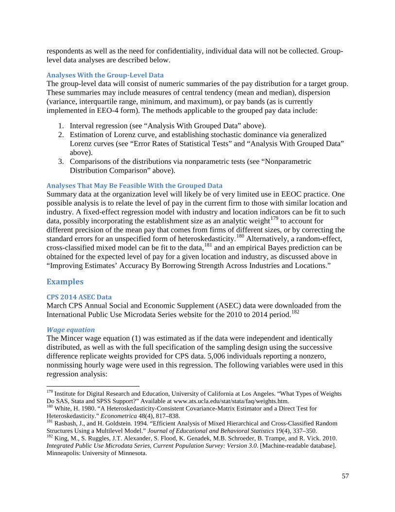
respondents as well as the need for confidentiality, individual data will not be collected. Group-level data analyses are described below.

Analyses With the Group-Level Data The group-level data will consist of numeric summaries of the pay distribution for a target group. These summaries may include measures of central tendency (mean and median), dispersion (variance, interquartile range, minimum, and maximum), or pay bands (as is currently implemented in EEO-4 form). The methods applicable to the grouped pay data include:

1. Interval regression (see “Analysis With Grouped Data” above). 2. Estimation of Lorenz curve, and establishing stochastic dominance via generalized

Lorenz curves (see “Error Rates of Statistical Tests” and “Analysis With Grouped Data” above).

3. Comparisons of the distributions via nonparametric tests (see “Nonparametric Distribution Comparison” above).

Analyses That May Be Feasible With the Grouped Data Summary data at the organization level will likely be of very limited use in EEOC practice. One possible analysis is to relate the level of pay in the current firm to those with similar location and industry. A fixed-effect regression model with industry and location indicators can be fit to such data, possibly incorporating the establishment size as an analytic weight179 to account for different precision of the mean pay that comes from firms of different sizes, or by correcting the standard errors for an unspecified form of heteroskedasticity.180 Alternatively, a random-effect, cross-classified mixed model can be fit to the data,181 and an empirical Bayes prediction can be obtained for the expected level of pay for a given location and industry, as discussed above in “Improving Estimates’ Accuracy By Borrowing Strength Across Industries and Locations.”

Examples

CPS 2014 ASEC Data March CPS Annual Social and Economic Supplement (ASEC) data were downloaded from the International Public Use Microdata Series website for the 2010 to 2014 period.182

Wage equation The Mincer wage equation (1) was estimated as if the data were independent and identically distributed, as well as with the full specification of the sampling design using the successive difference replicate weights provided for CPS data. 5,006 individuals reporting a nonzero, nonmissing hourly wage were used in this regression. The following variables were used in this regression analysis:

179 Institute for Digital Research and Education, University of California at Los Angeles. “What Types of Weights Do SAS, Stata and SPSS Support?” Available at www.ats.ucla.edu/stat/stata/faq/weights.htm. 180 White, H. 1980. “A Heteroskedasticity-Consistent Covariance-Matrix Estimator and a Direct Test for Heteroskedasticity.” Econometrica 48(4), 817–838. 181 Rasbash, J., and H. Goldstein. 1994. “Efficient Analysis of Mixed Hierarchical and Cross-Classified Random Structures Using a Multilevel Model.” Journal of Educational and Behavioral Statistics 19(4), 337–350. 182 King, M., S. Ruggles, J.T. Alexander, S. Flood, K. Genadek, M.B. Schroeder, B. Trampe, and R. Vick. 2010. Integrated Public Use Microdata Series, Current Population Survey: Version 3.0. [Machine-readable database]. Minneapolis: University of Minnesota.

57

1. Control variables: a. Identifiers of industry: It is unclear whether CPS uses a standard scheme such as

NAICS; the original four-digit variable with 261 unique values was recoded into two-digit variable by dropping the last two digits, producing 92 unique values, of which 90 values occur with the usable wage data.

b. Identifiers of occupation: CPS uses a 4-digit coding scheme with 484 unique values; they were recoded to a 2-digit variable by dropping the last 2 digits, producing 99 unique values, of which 98 values occur with the usable wage data.

c. Education: The five categories used were below high school, high school/GED, some college, bachelor’s degree, and professional or doctoral degree.

d. Class of worker: Four values across the usable wage data were used: wage/salary with private employers, federal government, state government, and local government.

2. Design/demographic variables: a. Sex. b. Race/ethnicity: The categories used were non-Hispanic white, non-Hispanic

black, non-Hispanic Asian, non-Hispanic all other races or multiple races, and Hispanic.

c. Interaction of sex and race.

The results of the wage equation estimation are reported in Table 1. Three regressions were run with no survey design specifications and with full survey design settings. The coding of sex and race/ethnicity is in terms of the main effects. Sufficient degrees of freedom exist in the unweighted regression. In the regression that accounts for survey design, the survey design degrees of freedom are based on the number of replicate weights provided for CPS data, which is equal to 160. This number is exceeded with the specifications that involve control variables, so the standard errors may need to be treated with caution. Comparison of the specification with demographic variables only (columns 2 and 5) and control + demographic variables (columns 3 and 6) illustrates the danger of not having enough controls. When only the demographic variables are being used, black race and Hispanic ethnicity appear with significantly negative coefficients, implying that these groups are paid less than the reference group (white males). However, once additional controls are added, the effect of race/ethnicity is reduced, with the effect explained by the differences in education and occupations among these demographic groups. Coefficients for females are consistently negative: –13 percent in the demographics-only specification (overstating the effect) and –10 percent with the appropriate controls for industry, occupation, and education. The estimate of the coefficient for black race indicates pay reduced by14 percent (highly significant) to 7.5 percent (significant only at the 5% level).

Table 1. Results of wage equation estimation, with 95% CI. Unweighted (assumed independent and

identically distributed) Accounting for survey design

Control only

Design only Control + design

Control only

Design only Control + design

White male Base Base Base Base Base Base Black race -0.129*** -0.052 -0.137** -0.075* [ -0.202,-

0.055] [ -0.115, 0.012]

[-0.221, -0.053]

[-0.146,-0.004]

58

Asian race -0.019 0.007 -0.015 0.011 [-0.115,

0.077] [-0.071, 0.086]

[-0.115,0.086] [-0.067, 0.088]

Other race -0.086 -0.060 -0.119 -0.089 [-0.221,

0.050] [-0.164, 0.045]

[-0.268,0.030] [-0.209,0.032]

Hispanic race -0.187*** -0.040 -0.185*** -0.047 [-0.237, -

0.137] [-0.090, 0.010]

[-0.234,-0.136]

[-0.104,0.010]

Female -0.134*** -0.096*** -0.133*** -0.102*** [-0.168, -

0.100] [-0.129, -0.063]

[-0.168,-0.098]

[-0.135,-0.069]

Black female 0.057 0.036 0.048 0.045 [-0.036,

0.150] [-0.044, 0.115]

[-0.050, 0.146]

[-0.042,0.133]

Asian female 0.073 0.075 0.096 0.051 [-0.061,

0.207] [-0.030, 0.181]

[-0.036, 0.229]

[-0.055,0.157]

Other female -0.090 -0.081 -0.124 -0.066 [-0.273,

0.092] [-0.221, 0.059]

[-0.335, 0.088]

[-0.244, 0.111]

Hispanic female

0.040 0.038 0.038 0.052

[-0.030, 0.109]

[-0.024, 0.100]

[-0.030, 0.105]

[-0.013, 0.116]

R2 0.423 0.032 0.431 0.414 0.034 0.422 Var[residual] 0.1489 0.2408 0.1473 n/a n/a D.f. per parameter

25.9 556.2 24.8 n/a n/a n/a

Note: Dummy variables for 92 industries, 98 occupations, 5 education groups and 4 class of worker groups are incorporated in the specifications “Control” and “Control + Design.” The entries are regression coefficients and 95% confidence intervals. *Significant at 5% level; **Significant at 1% level; ***Significant at 0.1% level.

Wage and salary income corrected for hours worked To illustrate how the correction of the total wage and salary income for hours worked can be developed, the regression model was fit to a different set of variables and a different set of CPS respondents who provided the data. Using a much larger sample of 61,617 individuals, we analyzed the log of wage and salary income as the dependent variable and the sum of logs of the usual hours worked per week and weeks worked last year (the sum of logs is the log of the approximate total hours worked last year) as regression offset. The coefficient of the latter variable was restricted to be negative one, effectively providing the interpretation of the model as a whole as the effective pay rate per hour. The results are provided in Table 2.

59

Table 2. Results of estimation for wage/salary income corrected for hours worked. Unweighted (assumed independent and identically distributed) Offset

only Control only

Design only Control + design Control + design + FTE

White male Not used

Not used

Base Base Base

Black race -0.261 -0.120 -0.117 [-0.291,-0.231]*** [-0.146,-0.093]*** [-0.143,-0.091]*** Asian race 0.011 -0.068 -0.072 [-0.028,0.051] [-0.101,-0.036]*** [-0.104,-0.041]*** Other race -0.246 -0.093 -0.089 [-0.298,-0.194]*** [-0.138,-0.049]*** [-0.133,-0.045]*** Hispanic race -0.367 -0.101 -0.108 [-0.387,-0.347]*** [-0.119,-0.082]*** [-0.126,-0.089]*** Female -0.240 -0.185 -0.178 [-0.255,-0.224]*** [-0.200,-0.170]*** [-0.193,-0.163]*** Black female 0.110 0.064 0.055 [0.069,0.150]*** [0.029,0.099]*** [0.021,0.090]** Asian female 0.072 0.100 0.098 [0.017,0.127]* [0.056,0.144]*** [0.054,0.142]*** Other female 0.107 0.052 0.044 [0.035,0.179]** [-0.010,0.114] [-0.018,0.105] Hispanic female

0.097 0.066 0.070

[0.068,0.126]*** [0.041,0.092]*** [0.045,0.096]*** Full-time work F(10,61399)=106.99 R2 0 0.354 0.046 0.363 0.377 D.f. per parameter

311.2 7242.6 297.7 283.9

Var[residual] 0.6289 0.4061 0.6003 0.4004 0.3919 Accounting for survey design Offset

only Control only

Design only Control + design Control + design + FTE

White male Not used

Not used

Base Base Base

Black race -0.283 -0.124 -0.120 [-0.316,-0.249]*** [-0.152,-0.096]*** [-0.148,-0.093]*** Asian race 0.054 -0.057 -0.063 [0.005,0.102]* [-0.097,-0.017]** [-0.101,-0.024]** Other race -0.276 -0.114 -0.108 [-0.350,-0.203]*** [-0.177,-0.051]*** [-0.170,-0.046]*** Hispanic race -0.387 -0.117 -0.124 [-0.413,-0.361]*** [-0.138,-0.095]*** [-0.146,-0.103]*** Female -0.227 -0.177 -0.171 [-0.245,-0.209]*** [-0.196,-0.158]*** [-0.190,-0.152]*** Black female 0.108 0.056 0.048 [0.063,0.152]*** [0.019,0.093]** [0.013,0.084]** Asian female 0.018 0.070 0.074 [-0.040,0.077] [0.021,0.120]** [0.025,0.122]**

60

Other female 0.132 0.061 0.052 [0.049,0.216]** [-0.017,0.139] [-0.023,0.127] Hispanic female

0.108 0.074 0.080

[0.075,0.141]*** [0.043,0.104]*** [0.050,0.110]*** Full-time work 𝜒𝜒2(10) = 765.00 Note: Dummy variables for 92 industries, 98 occupations, 5 education groups and 4 class of worker groups are incorporated in all the specifications with “Control.” Six dummy variables for weeks worked last year and the interaction of hours worked per week with full-time status (<35 hours/week, part time; 35 to 50 hours/week, full time; >50 hours/week, overtime) are incorporated in the “Control + design + FTE” specifications. Coefficient of the total hours worked last year is constrained to –1. The entries are regression coefficients and 95% confidence intervals. *Significant at 5% level; **Significant at 1% level; ***Significant at 0.1% level.

One immediate observation is that the demographic variables are highly significant in all specifications, with main effects of race/ethnicity and gender suggesting significantly lower incomes. The interactions of race/ethnicity and female, however, are all positive and significant, except for other female, although the magnitudes are all lower than the main effect of gender; that is, nonwhite females earn less than nonwhite males in the same race/ethnicity group, but the difference from the males in their respective race/ethnicity group is smaller than the difference between white males and females. Accounting for survey design and reweighting of the demographic groups reduced the significance of some of these demographic variables. To investigate sensitivity to the assumption of a linear relation between the total hours worked in a year and the total wage/salary compensation, additional variables were introduced in the last column: six dummy variables for weeks worked last year (1–13 weeks, 14–26 weeks, 27–39 weeks, 40–47 weeks, 48–49 weeks, 50–52 weeks), and the interaction of hours worked per week with the full-time status (coded with three categories: <35 hours/week, part time; 35 to 50 hours/week, full time; and >50 hours/week, overtime). With these variables included, the R2 improved somewhat, but the coefficients of the demographic variables remained mostly unchanged (in the survey regression, nearly uniformly by a factor of two). The coefficients of these additional variables (not reported) indicated that the compensation of workers who did not work the full year was approximately 10 percent lower per hour whenever they worked fewer than 50 weeks. The economic interpretation of this finding is that employers provide higher compensation per hour (that is, disproportionately higher total compensation) to the permanent employees. The effect of hours per week was inconclusive (see Figure 5). Although the stability of the demographic coefficients between the last two columns is encouraging, we have to recognize the varying patterns of compensation for employees who work different hours. As a result, pooling together into a single cell the employees who may have received the same compensation from working different hours, and analyzing them with a single offset as the format of the proposed EEOC form suggests, may lead to biases that are difficult to quantify because of the model misspecification with respect to the time commitments required by the different positions.

61

Figure 6. Differences in pay per hour as a function of the number of hours worked in a week.

62

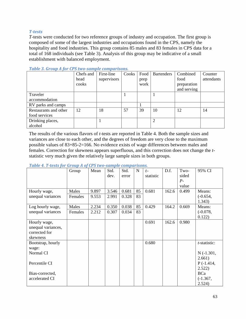
T-tests T-tests were conducted for two reference groups of industry and occupation. The first group is composed of some of the largest industries and occupations found in the CPS, namely the hospitality and food industries. This group contains 85 males and 83 females in CPS data for a total of 168 individuals (see Table 3). Analysis of this group may be indicative of a small establishment with balanced employment.

Table 3. Group A for CPS two-sample comparisons. Chefs and

head cooks

First-line supervisors

Cooks Food prep work

Bartenders Combined food preparation and serving

Counter attendants

Traveler accommodation

1 1

RV parks and camps 1 Restaurants and other food services

12 18 57 39 10 12 14

Drinking places, alcohol

1 2

The results of the various flavors of t-tests are reported in Table 4. Both the sample sizes and variances are close to each other, and the degrees of freedom are very close to the maximum possible values of 83+85-2=166. No evidence exists of wage differences between males and females. Correction for skewness appears superfluous, and this correction does not change the t-statistic very much given the relatively large sample sizes in both groups.

Table 4. T-tests for Group A of CPS two-sample comparisons. Group Mean Std.

dev. Std. error

N 𝑡𝑡-statistic

D.f. Two-sided P-value

95% CI

Hourly wage, unequal variances

Males 9.897 3.546 0.681 85 0.681 162.6 0.499 Means: (-0.654, 1.343)

Females 9.553 2.991 0.328 83

Log hourly wage, unequal variances

Males 2.234 0.350 0.038 85 0.429 164.2 0.669 Means: (-0.078, 0.122)

Females 2.212 0.307 0.034 83

Hourly wage, unequal variances, corrected for skewness

0.691 162.6 0.980

Bootstrap, hourly wage: Normal CI Percentile CI Bias-corrected, accelerated CI

0.680 t-statistic: N (-1.301, 2.661) P (-1.414, 2.522) BCa (-1.367, 2.524)

63

The second group used in comparisons of males and females is the group of elementary and secondary school teachers, which consisted of 4 males and 22 females (see Table 5). It thus represents a small sample that is heavily unbalanced by gender. A somewhat protective effect is offered by the smaller variance (8.58 vs. 10.05) of the smaller group (males). Still, the Satterthwaite degrees of freedom pretty much correspond to the smallest sample size (4.64 for comparisons of mean levels of pay, 6.10 for comparisons of the mean levels of logs). Correction for skewness produces a more pronounced effect on the test statistic than in the previous group and results in a p-value that is very similar to that in the t-test of logs. Imbalance and asymmetry of the situation are especially vividly seen in the difference of the bootstrap confidence intervals; although the bootstrap bias correction brings the t-statistic down, both percentile and bias-corrected intervals bring the confidence limits up compared with the symmetric normal interval. The implicit p-values from these confidence intervals are below 0.05, because they do not cover zero.

Table 5. T-tests for Group B of CPS two-sample comparisons. Group Mean Std.

dev. Std. error

N 𝑡𝑡-statistic

D.f. Two-sided P-value

95% CI

Hourly wage, unequal variances

Males 30.94 8.58 4.292 4 1.697 4.64 0.155 Mean: (-4.484, 20.76)

Females 22.80 10.05 2.142 22

Log hourly wage, unequal variances

Males 3.403 0.276 0.138 4 2.208 6.10 0.069 Mean: (-0.039, 0.770)

Females 3.037 0.432 0.092 22

Hourly wage, unequal variances, corrected for skewness

1.824 4.64 0.132

Bootstrap, hourly wage: Normal CI Percentile CI Bias-corrected, accelerated CI

1.516 t-statistic: N (-0.288, 3.320) P (0.083, 3.617) BCa (0.086, 3.644)

Distribution comparison tests Nonparametric tests were conducted for the two groups identified in the previous sections. The results are given in Table 6. This analysis unveiled differences in a categorical variable of race/ethnicity that has more than two levels (and therefore is not amenable to modified t-tests or Kolmogorov-Smirnov tests) in the first group. These analyses were conducted on unweighted data, which is inappropriate for CPS given its complex survey design.

64

Table 6. Nonparametric distribution comparison tests for subsets of CPS data. CPS subset Factor Kolmogorov-

Smirnov p-value Kruskal-Wallis

p-value Group A: food industry Gender 0.715 0.6219 Race/ethnicity N/A 0.001 Gender by race/ethnicity N/A 0.018 Group B: elementary and secondary schools

Gender 0.158 0.094

Permutation tests For permutation testing, several implementation options should be considered. Either the outcome variables (pay) or the variables of interest (demographics) can be permuted. Permutations can be carried out for the full data set, or within cells identified by the control variables (industry, location, job category). We produced permutation analogues of t-tests to compare mean pay across sex as well as an analysis of variables with multiple categories through ANOVA. Because permutation testing works best for one-sided rejection regions, the appropriate permutation test statistic to compare means of two groups is the total for one of the groups.183 The rejection region for F-statistics is already of the form “F > critical value,” so the ANOVA F-statistic was permuted with no modifications. One thousand permutations were taken in each of the analyses. The results are reported in Table 7. They are qualitatively comparable to the findings reported above.

Table 7. Permutation testing of differences between demographic groups in subsets of CPS data. CPS subset Analysis and statistic permuted Permutation by… p-value Group A: Food industry

Total, males, unweighted Outcome (hourly wage) 0.262 Total, males, using survey weights Outcome (hourly wage) 0.079 ANOVA (hourly wage on sex), unweighted, F-statistic

Outcome (hourly wage) 0.473

ANOVA (hourly wage on sex), unweighted, F-statistic

Demographic variable (sex) 0.495

ANOVA (hourly wage on race/ethnicity), unweighted, F-statistic

Outcome (hourly wage) 0.032

ANOVA (hourly wage on sex), unweighted, F-statistic

Demographic variable (sex by race/ethnicity interaction)

0.177

Group B: Elementary and secondary schools

Total, males, unweighted Outcome (hourly wage) 0.069 Total, males, using survey weights Outcome (hourly wage) 0.042 ANOVA (hourly wage on sex), F-statistic

Outcome (hourly wage) 0.139

ANOVA (hourly wage on sex), F-statistic

Demographic variable (sex) 0.155

Permutation can also be applied in regression analysis. We applied permutation of the outcome for the regression model with survey design in control + design model specification, last column of Table 1. The permuted statistic was the Wald test for whether the coefficient of sex is equal to

183 Good 2005, pp. 51–54.

65

zero (that is, the square of the t-statistic, the ratio of the coefficient estimate to its standard error). In none of the 1,000 replicates did the permuted statistic exceed its observed value, resulting in the permutation p-value < 0.001.

The permutation testing approach provides for a simple visualization via plots of the permuted values with overlaid observed values and the graphical interpretation of the p-value. These distributions are simulated sampling distributions of the test statistics under the null, and they include the potential deviations from the standard reference distributions due to nonnormality, small cell sizes, and so on. The distribution of the total in Figure 6(a) is approximately normal, whereas the distribution of the F-statistic in Figure 6(b) shows the features of the F-distribution with one degree of freedom in the numerator (a vertical asymptote of the density near 0, long right tail). The p-values are based on the counts of the number of permuted samples that produced values greater than the observed ones, which are shown by vertical lines on the plots.

66

(a) Permutation test statistic = total for males (Group A, outcome = hourly wage).

(b) Permutation test statistic = F-statistics from ANOVA (Group A, outcome = hourly wage).

Figure 7. Permutation distributions of the test statistics.

p-value = % to the right0

2.0e

-06

4.0e

-06

6.0e

-06

Den

sity

1900000 2000000 2100000 2200000 2300000 2400000Weighted total

p-value = .079

p-value = % to the right

0.5

11.

5D

ensi

ty

0 2 4 6 8 10ANOVA F-statistic

p-value = .473

67

Summary of the findings Table 8 summarizes the findings, reporting the lowest and the highest p-values across the various tests reported in the previous sections.

Table 8. Summary of the testing of differences between demographic groups in subsets of CPS data. CPS subset Factor Lowest p-value Highest p-value Group A: Food industry

Gender 0.079 (permutation test, weighted means)

0.715 (Kolmogorov-Smirnov test of equality of distributions,

unweighted) Race/ethnicity 0.001

(Kruskal-Wallis non-parametric ANOVA,

unweighted)

0.155 (t-test assuming unequal variances, no skewness

corrections, unweighted) Gender by race/ethnicity 0.018

(Kruskal-Wallis non-parametric ANOVA,

unweighted)

0.177 (permutation test,

unweighted)

Group B: Elementary and secondary schools

Gender 0.042 (permutation test, weighted means)

0.158 (Kolmogorov-Smirnov test of equality of distributions,

unweighted)

Power analysis with continuous data Ad-hoc power analysis was conducted with the estimates from the full survey specification of the control + design regression specification reported in Table 1, with standard errors accounting for the survey design effects. The power curves for the traditional 1% and 5% levels of significance are shown in Figure 7. Only for the medium size companies with several hundred employees does the power exceed 50 percent.

68

Figure 8. Power curves for detecting the 10% difference of female wages/salaries.

As argued above in “Error Rates of Statistical Tests,” an alternative view on the issue of error rates and power may involve fixing the effect size and the target power and varying the significance level (or the size of the test) with the sample size (establishment size) to equate enforcement efforts across the spectrum of company sizes. The significance levels that would equate the power of the test are shown in Figure 8. The significance level is the fraction of companies that do not discriminate that will be flagged for investigation, which is a measure of operational efficiency. A high rate of type I error may be wasteful.

69

Figure 9. Significance level of the tests for detecting the 10% difference of female wages/salaries at a given power.

Mixed/multilevel model analysis As discussed previously, multilevel models can be used to incorporate a large number of random effects for locations, industries, or occupations to borrow strength across establishments that share similar characteristics. Specification (24) with cross-classified random effects of location (51 states and the District of Columbia), industry (90 values of ind100 variable) and occupation (99 values of occ100 variable) was run, with the results reported in Table 9 (which is directly comparable with Table 1). Weights were not included because weighted estimation with cross-classified models is not supported. As with the linear regression model, the mixed multilevel model finds that the wages/salaries of females are about 10% lower than those of males. Weaker evidence exists that the wages/salaries of Hispanic employees are lower than those of the reference group (white males).

Table 9. Mixed effect modeling of the wage equation with CPS data. Unweighted (assumed independent and identically

distributed) Control only Control + design

White male Base Base Black race -0.054

[-0.111,0.004] Asian race -0.011

[-0.086,0.064] Other race -0.074

.000

1.0

01.0

1.1

.5S

igni

fican

ce le

vel

30 100 300 1000 3000 10000Sample size

Power = 50% Power = 80% Power = 90%

70

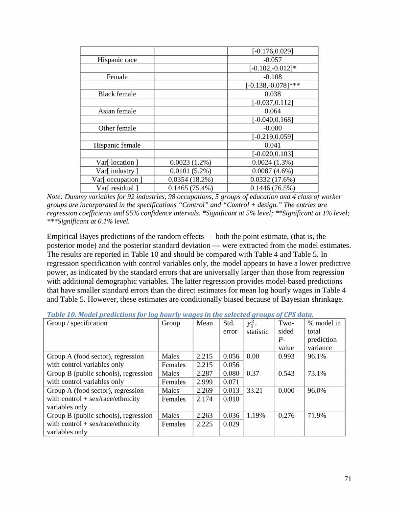
[-0.176,0.029] Hispanic race -0.057

[-0.102,-0.012]* Female -0.108

[-0.138,-0.078]*** Black female 0.038

[-0.037,0.112] Asian female 0.064

[-0.040,0.168] Other female -0.080

[-0.219,0.059] Hispanic female 0.041

[-0.020,0.103] Var[ location ] 0.0023 (1.2%) 0.0024 (1.3%) Var[ industry ] 0.0101 (5.2%) 0.0087 (4.6%)

Var[ occupation ] 0.0354 (18.2%) 0.0332 (17.6%) Var[ residual ] 0.1465 (75.4%) 0.1446 (76.5%)

Note: Dummy variables for 92 industries, 98 occupations, 5 groups of education and 4 class of worker groups are incorporated in the specifications “Control” and “Control + design.” The entries are regression coefficients and 95% confidence intervals. *Significant at 5% level; **Significant at 1% level; ***Significant at 0.1% level.

Empirical Bayes predictions of the random effects — both the point estimate, (that is, the posterior mode) and the posterior standard deviation — were extracted from the model estimates. The results are reported in Table 10 and should be compared with Table 4 and Table 5. In regression specification with control variables only, the model appears to have a lower predictive power, as indicated by the standard errors that are universally larger than those from regression with additional demographic variables. The latter regression provides model-based predictions that have smaller standard errors than the direct estimates for mean log hourly wages in Table 4 and Table 5. However, these estimates are conditionally biased because of Bayesian shrinkage.

Table 10. Model predictions for log hourly wages in the selected groups of CPS data. Group / specification Group Mean Std.

error 𝜒𝜒12-statistic

Two-sided P-value

% model in total prediction variance

Group A (food sector), regression with control variables only

Males 2.215 0.056 0.00 0.993 96.1% Females 2.215 0.056

Group B (public schools), regression with control variables only

Males 2.287 0.080 0.37 0.543 73.1% Females 2.999 0.071

Group A (food sector), regression with control + sex/race/ethnicity variables only

Males 2.269 0.013 33.21 0.000 96.0% Females 2.174 0.010

Group B (public schools), regression with control + sex/race/ethnicity variables only

Males 2.263 0.036 1.19% 0.276 71.9% Females 2.225 0.029

71

Note that although the methodology is widely used in areas ranging from educational research (to model the hierarchical structures of districts, schools, classes, and students nested one into another) to biostatistics (to model visits nested in patients nested in clinics), economists tend to rely on fixed-effects methods (as exemplified by the default regression model (1) with the full set of dummy variables for locations, industries and occupations) rather than random-effects methods. In many panel data econometric applications, random-effect models are often found to fail Hausman specification tests and therefore are at risk of producing biased estimates of regression parameters.184

Optimal grouping of incomes Davies and Shorrocks’ optimal grouping procedure to maximize the Gini index of the grouped data was applied to the CPS data for total wage and salary income (incwage) because it provides the economy-wide distribution of labor incomes.185 First, the search for the bounds of the optimal partition was implemented on the full data set of 65,183 individuals with nonzero wage and salary incomes for groups of 8, 10, 12, 15, and 20. The first part of Davies-Shorrocks algorithm provides the lower and upper bounds on the partitions that satisfy the optimality conditions of distorting inequality as little as possible. Within the first part of the algorithm, the possible cutoff points are enumerated from the bottom of the distribution up, in an optimized way guided by the mathematical properties of the distribution, to generate the lower bounds on the optimal cutoff points; and then the cutoff points are enumerated again from the top of the distribution down, to generate the upper bounds. The second part of the algorithm performs an exhaustive search within the bounds thus found to find the optimal grouping. Since most of the enumerated combinations satisfy the optimality conditions, the Gini index has to be computed for each considered combination of cutoff points. The computational load increases combinatorially with the sample size and the number of groups. The final weights were used in the analysis to ensure that the distribution is representative of the economy as a whole. The results are reported in Table 11.

184 Wooldridge 2010. 185 Davies and Shorrocks 1989.

72

Table 11. Upper cutoff points of the optimal groupings of wage and salary income in CPS data. Class Lower bound Upper bound Class Lower bound Upper bound

8 groups 15 groups 35 combinations compared 62 combinations compared 1 8986 13027 1 2137 10775 2 18175 25259 2 4776 21220 3 27907 38246 3 7758 31151 4 39412 52385 4 10940 41081 5 54738 72450 5 14792 50775 6 79693 102556 6 18817 61250 7 138500 184500 7 23547 72750 8 ∞ ∞ 8 29951 85900

10 groups 9 37174 103039 52 combinations compared 10 46494 126156 1 6753 10775 11 59648 157263 2 14445 21270 12 76650 207233 3 21378 31612 13 107501 312500 4 29157 42620 14 189500 575000 5 37915 55030 15 ∞ ∞ 6 49658 70763 20 groups 7 65890 91450 79 combinations compared 8 94363 127250 1 829 10775 9 164000 228500 2 1759 21220 10 ∞ ∞ 3 2955 31032

12 groups 4 4225 40970 60 combinations compared 5 5837 50468 1 5388 10775 6 7531 60746 2 11553 21220 7 9428 71101 3 17153 31187 8 11305 81550 4 22957 41454 9 13988 95126 5 29615 52475 10 16436 110807 6 37138 65950 11 19944 133410 7 46457 81350 12 23847 162250 8 59648 101847 13 29995 200501 9 76650 131300 14 37174 252000 10 107501 186178 15 46494 321500 11 189500 355000 16 59648 410000 12 ∞ ∞ 17 76650 525000 18 107501 722500 19 189500 980000 20 ∞ ∞

73

Table 12. Detailed upper cutoff points of the optimal groupings of wage and salary income in subsamples of the CPS data. Class Lower

bound Upper bound Optimal Class Lower

bound Upper bound

Optimal

8 groups (5% sample; n=3,256) 15 groups (2% sample; n=1,303) Run time = 4 hr 24 min; 757,571 combinations Run time = 14 hr 44 min; 1,141,950 combinations

1 9080 13625 11600 1 1290 11120 4975 2 18754 25450 22305 2 2880 21546 11620 3 27795 38111 33265 3 4841 30750 17250 4 39700 53500 46300 4 7751 40923 22250 5 56500 73200 64500 5 10828 51350 27750 6 83500 104500 92500 6 14580 62250 32550 7 143000 176500 155500 7 18700 74500 39251 8 ∞ ∞ ∞ 8 23160 90822 46578

10 groups (5% sample; n=3,256) 9 29688 111600 55750 Run time = 3 hr 40 min; 612,175 combinations 10 37489 132000 66500 1 8210 11270 8537 11 49350 155250 81348 2 16942 21550 17050 12 64500 192500 104000 3 24450 31412 24930 13 93500 265000 137500 4 32880 42061 33126 14 155250 525000 212500 5 43500 55750 43500 15 ∞ ∞ ∞ 6 56500 70564 57750 20 groups (1% sample; n=651) 7 74500 92500 75501 Run time = 5 hr 45 min; 2,419,605 combinations 8 105500 126000 107000 1 250 11500 3800 9 176500 217500 179500 2 441 22250 8337 10 ∞ ∞ ∞ 3 850 31500 13198

12 groups (2% sample; n=1,303) 4 1750 41500 18500 Run time = 3 hr 31 min; 1,143,950 combinations 5 2880 51600 22750 1 3850 11120 6200 6 3300 61000 27250 2 8537 21546 14580 7 4725 72500 31500 3 13750 30750 20749 8 6700 87500 36750 4 18700 41500 27270 9 9800 110600 41500 5 23160 53500 34501 10 13750 132500 47500 6 29688 65750 43500 11 18500 155000 54000 7 37489 81348 53500 12 22750 189500 61000 8 49350 104000 66500 13 27750 212500 68275 9 64500 132000 84155 14 34501 237500 78195 10 93500 182500 116500 15 43500 275000 90822 11 155250 317500 182500 16 56250 307500 113100 12 ∞ ∞ ∞ 17 74000 332500 137500 18 108000 525000 164000 19 174000 725000 275000 20 ∞ ∞ ∞

The bounds clearly are not sufficiently tight to determine the optimal allocation. To obtain one, a subsample of CPS data was taken to reduce the computational burden (the algorithms did not

74

converge within 12 hours), and the extension discussed by Davies and Shorrocks to obtain the optimal solution was implemented for these subsamples. The results are reported in Table 12.186

The lower and upper bounds differ from those in Table 11 because of subsampling variability. The optimal grouping in the last column provides the cutoff between income groups at which the income inequality of the distribution of the total wage and salary income, as expressed by the Gini coefficient, is best preserved. For practical purposes, the numbers could be rounded or truncated down. The distribution of CPS wage and salary income reflects the total annual income that an individual may have received from multiple jobs, so if W-2 income is used in EEOC data collection, it may reflect only a part of the total income that an individual received in the part of the year they worked for a given establishment. For example, with 10 groups, the brackets could be defined as $0 to $7,999, $8,000 to $16,999, $17,000 to $24,999, $25,000 to $32,999, $33,000 to $42,999, $43,000 to $56,999, $57,000 to $74,999, $75,000 to $104,999, $105,000 to $179,999, and $180,000 and above.

The challenges that we encounter are computational. CPS March Supplement (ASEC) by itself is the representative data set of the U.S. economy, but implementing the algorithm on the full data set is nearly impossible as computation time increases combinatorially fast (i.e., faster than exponentially; more like 𝑂𝑂(𝑙𝑙!) ∼ 𝑂𝑂(𝑙𝑙𝑙𝑙/e𝑙𝑙) than 𝑂𝑂(𝑙𝑙𝑘𝑘) or 𝑂𝑂(𝐸𝐸𝑙𝑙).) The optimization task only needs to be performed once, though, so running the algorithm on a larger subset of CPS on a more powerful computer remains a possibility.

The quality of approximation of the earnings distribution by the categorical versions is gauged by Figure 9 that plots Lorenz curves based on the original and discretized earnings data. Midpoints of the intervals were imputed for the interior points. The value of $115,000 was imputed for the upper range of EEO-4 brackets, and the value of $235,000 was imputed for the upper range of the proposed brackets, so that the mean incomes with the imputed variables match the original mean income. Clearly, while capturing the major aspects of the earnings distribution, both versions clearly underestimate inequality in it, as they lie strictly above the Lorenz curve based on the original data.

186 Davies and Shorrocks 1989.

75

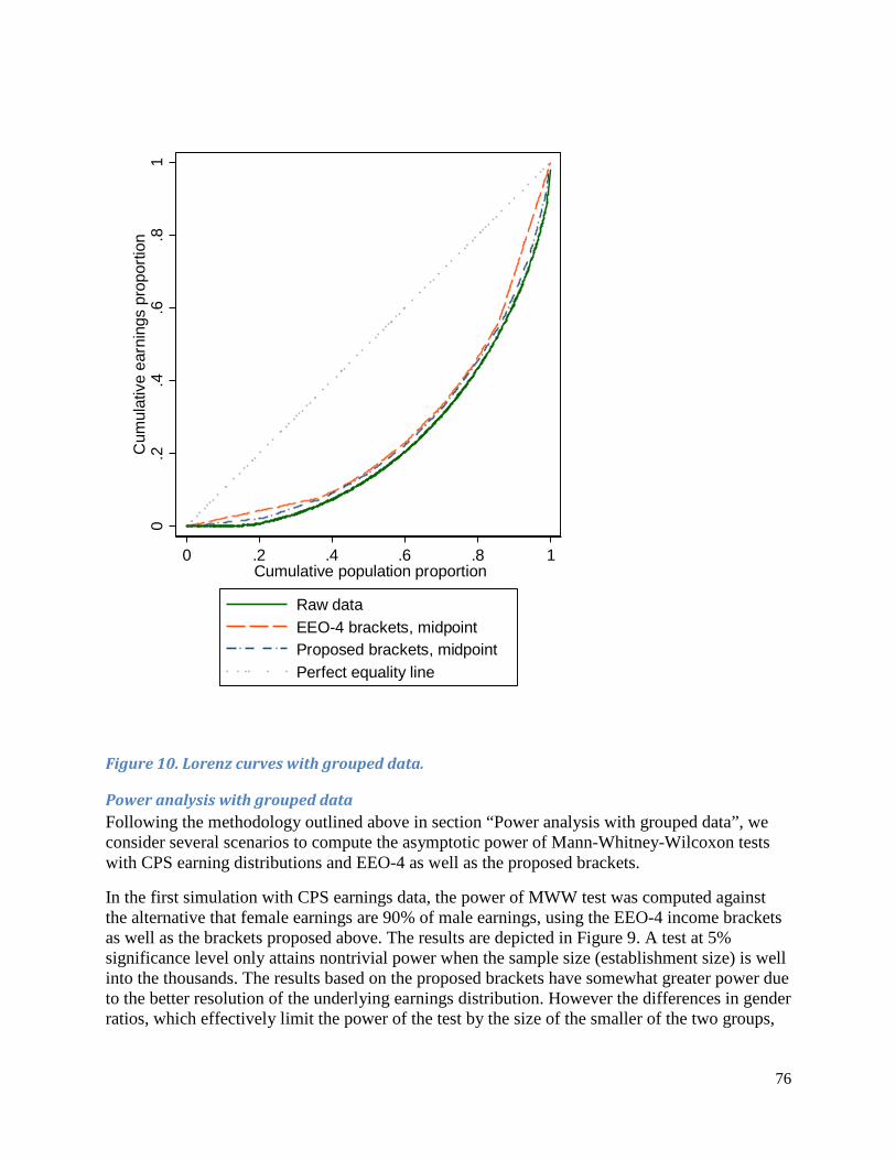
Figure 10. Lorenz curves with grouped data.

Power analysis with grouped data Following the methodology outlined above in section “Power analysis with grouped data”, we consider several scenarios to compute the asymptotic power of Mann-Whitney-Wilcoxon tests with CPS earning distributions and EEO-4 as well as the proposed brackets.

In the first simulation with CPS earnings data, the power of MWW test was computed against the alternative that female earnings are 90% of male earnings, using the EEO-4 income brackets as well as the brackets proposed above. The results are depicted in Figure 9. A test at 5% significance level only attains nontrivial power when the sample size (establishment size) is well into the thousands. The results based on the proposed brackets have somewhat greater power due to the better resolution of the underlying earnings distribution. However the differences in gender ratios, which effectively limit the power of the test by the size of the smaller of the two groups,

0.2

.4.6

.81

Cum

ulat

ive

earn

ings

pro

porti

on

0 .2 .4 .6 .8 1Cumulative population proportion

Raw dataEEO-4 brackets, midpointProposed brackets, midpointPerfect equality line

76

also have a pronounced effect on the power of the test, with unbalanced groups producing tests of lower power.

While having the advantage of utilizing the economy-wide, nation-wide distribution of earnings, the analysis with CPS data does not condition on control variables, i.e., does not take into account the potentially different demographic compositions of different occupations and job groups. Earning distributions within more tightly defined economic groups are tighter; while the coefficient of variation (ratio of the standard deviation to the mean, a common measure of dispersion for skewed distributions) is about 1 for the CPS distribution as a whole, it is much lower within job groups, with typical values of 0.1 to 0.2.

To analyze the power of the MWW test in these circumstances, we simulated earnings data from lognormal distributions with standard deviation of logs (approximately equal to the coefficient of variation) of 0.2, and the distribution means of $20,000, $50,000 and $80,000. As the EEO-4 income brackets are somewhat more detailed at lower levels, the EEO-4 brackets provide better power for the group of $20,000. As the proposed brackets are more detailed at higher levels of earnings, they provide better power for higher earnings for the group with mean earnings of $80,000. The instruments perform about the same for the middle value of $50,000.

Figure 11. Power of Mann-Whitney-Wilcoxon test for CPS data.

0.2

.4.6

.81

5 10 20 50 100 200 500 1000 2000n

EEO-4 brackets; 1:4 gender EEO-4 brackets; 1:1 genderProposed brackets; 1:4 gender Proposed brackets; 1:1 gender

Discrimination earnings ratio = 90%; significance = 5%

77

Figure 12. Power of Mann-Whitney-Wilcoxon test; mean earnings = $20,000, CV=0.2.

Figure 13. Power of Mann-Whitney-Wilcoxon test; mean earnings = $50,000, CV=0.2.

0.2

.4.6

.81

5 10 20 50 100 200 500 1000 2000n

EEO-4 brackets; 1:4 gender EEO-4 brackets; 1:1 genderProposed brackets; 1:4 gender Proposed brackets; 1:1 gender

Discrimination earnings ratio = 90%; significance = 5%Simulated lognormal mean = $ 20000, CV=20%

0.2

.4.6

.81

5 10 20 50 100 200 500 1000 2000n

EEO-4 brackets; 1:4 gender EEO-4 brackets; 1:1 genderProposed brackets; 1:4 gender Proposed brackets; 1:1 gender

Discrimination earnings ratio = 90%; significance = 5%Simulated lognormal mean = $ 50000, CV=20%

78

Figure 14. Power of Mann-Whitney-Wilcoxon test; mean earnings = $80,000, CV=0.2.

Simulated EEOC Data To analyze realistic person-level data that can be encountered within a company, SAS code was written to simulate pay data. The simulation code creates a realistic employment structure that reflects the average racial/ethnic and gender composition of job groups in industry. Then the Standard Occupational Classification (SOC) job codes are assigned using stratified sampling / hot deck from the existing structure of these codes. Finally, wages are imputed by hot deck from distributions of the OES wages within a given SOC category. See “Simulation Background” memo provided elsewhere for full description. The data set generated with the seed 3344 (wages_e2012_oes2013_n3344.sas7bdat) was used in the subsequent analysis. The gender composition of this simulated firm is given in Table 13. Males dominate in higher paid executive, managerial and professional jobs, while females dominate lower paid clerical and operator jobs. The simulated firm employs workers of 77 occupations.

Table 13. Composition of the workforce employed by the simulated firm. Job groups MALE FEMALE Total Senior Executive 6 1 7 Middle Manager 27 7 34 Professional 79 24 103 Technical 29 6 35 Sales 4 1 5 Clerical 4 10 14 Craft 8 2 10 Operator 27 31 58

0.2

.4.6

.81

5 10 20 50 100 200 500 1000 2000n

EEO-4 brackets; 1:4 gender EEO-4 brackets; 1:1 genderProposed brackets; 1:4 gender Proposed brackets; 1:1 gender

Discrimination earnings ratio = 90%; significance = 5%Simulated lognormal mean = $ 80000, CV=20%

79

Laborer 3 3 6 Total 187 85 272

The differences in distributions of salaries of males and females across the firm are striking. As Figure 14 shows, both distributions are heavily right skewed, even after the log transformation, and there is a greater share of women who receive lower salaries in lower job categories, as shown in Table 13. The plots of generalized Lorenz curves (Figure 14) allow avoidance of crossings seen in the kernel density plot, which may make the latter somewhat more difficult to interpret, and clearly shows that females in the company earn less males.

0.2

.4.6

.8kd

ensi

ty ln

wag

es

10 11 12 13 14Log annual salary

Male Female

80

Figure 15. Kernel density estimates of annual salaries (in logs) in simulated data.

Figure 16. Generalized Lorenz curves by gender in simulated data.

Wage equation As the first benchmark step in the analysis, wage equation was fit to the simulated data. The results are shown in Table 14. The control variables in this regression are job type and occupation, truncated to the first two digits. Because demographic categories and salaries were assigned independently in the simulated data, it is reasonable to expect that the demographic variables will not be significant predictors of salary. The simulated data reproduce the qualitative results of CPS data, with females and Hispanics showing lower salaries; however, the inclusion of the control variables corrects these results, making the demographic predictors insignificant. There is also a substantially higher R2 and lower residual variance than in the CPS regression, although it should be noted that the CPS regression is fit across a variety of industries and locations. The full control + design specification approaches the lower suggested number of observations per parameter (13.60 in the current data set, compared with the rule of thumb of 10 per parameter).

020

4060

8010

0G

en. L

oren

z kw

ages

(by

gend

er)

0 .2 .4 .6 .8 1Cumulative population proportion

MALE FEMALE

81

Table 14. Wage equation for simulated data. Control only Design only Control + design

White male Base Base Base Female -0.371 -0.046 [-0.620,-0.122]** [-0.115,0.023] Black race -0.168 0.168 [-0.591,0.255] [-0.019,0.355] Hispanic -0.408 0.011 [-0.744,-0.072]* [-0.066,0.087] Asian race -0.050 -0.004 [-0.251,0.151] [-0.069,0.061] Black female -0.283 -0.204 [-0.910,0.344] [-0.429,0.021] Hispanic female 0.127 0.063 [-0.414,0.667] [-0.066,0.191] Asian female -0.006 0.010 [-0.394,0.382] [-0.112,0.132] R2 0.9344 0.6573 0.9374 Var[residual] 0.0325 0.4321 0.0319 D. f. per parameter 20.92 38.86 13.60 Note: *, significant at 5% level; **, significant at 1% level.

A version of wage equation was run in the quantile regression form. The quantile being predicted was the median. The coefficients in the regression have the interpretation of the differences in conditional medians; that is, by how much a median in the distribution of annual salaries differ between males and females if that is the only difference between the two employees. Because quantile regression does not make distributional assumptions (other than existence of a well-defined median of the population distribution), it was run both on the original annual salaries variable (scaled in thousands of dollars), shown in the top half of Table 15, and for the logs of salaries, as shown in the bottom half. The regression with demographic variables only identifies the pronounced difference between males and females, however, this difference disappears once the job categories and occupations are controlled for. Note however that in the final regression, the salaries of black employees have a median that is significantly higher than that of whites. The sums of absolute deviations in the last two rows of each block serve as the variant of the total and residual variance used in computing R2. It is clear that the regression with demographic variables only does not have as much explanatory power as the models with job categories and occupations do.

82

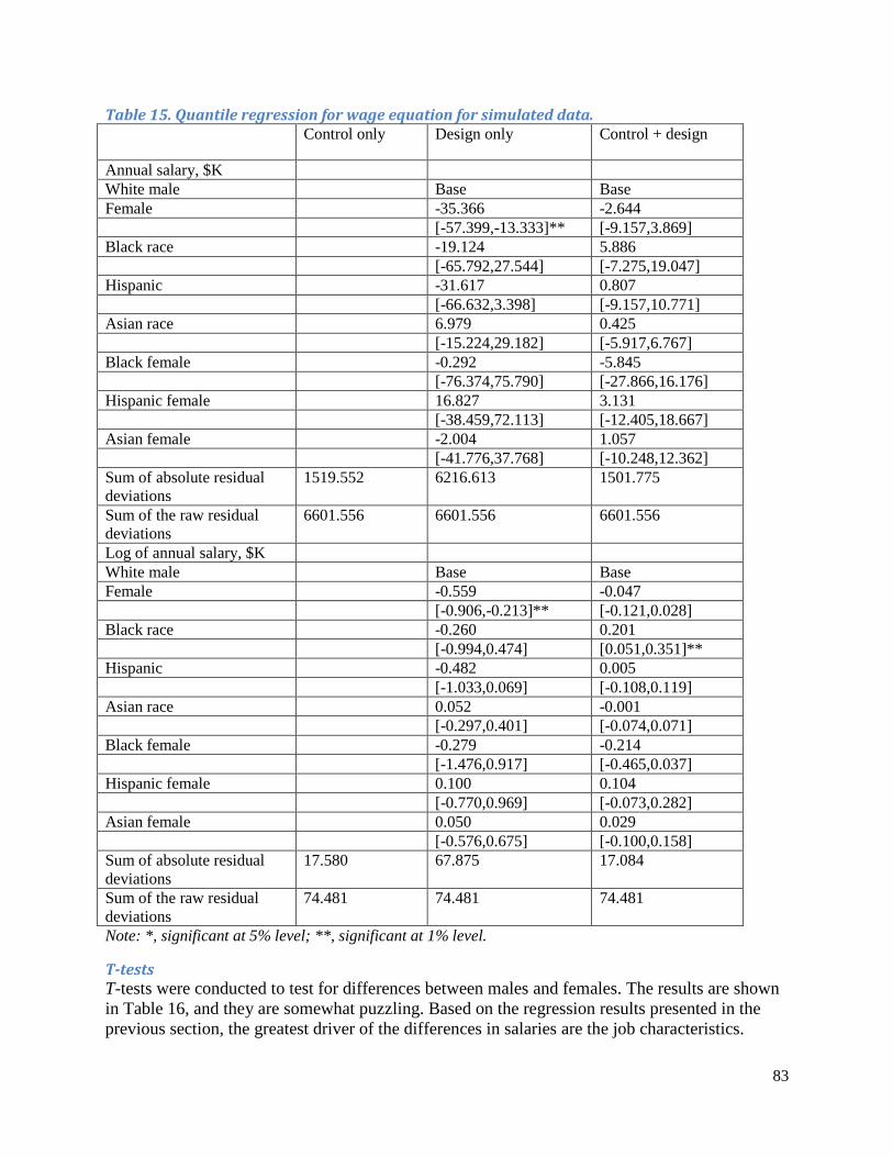
Table 15. Quantile regression for wage equation for simulated data. Control only Design only Control + design

Annual salary, $K White male Base Base Female -35.366 -2.644 [-57.399,-13.333]** [-9.157,3.869] Black race -19.124 5.886 [-65.792,27.544] [-7.275,19.047] Hispanic -31.617 0.807 [-66.632,3.398] [-9.157,10.771] Asian race 6.979 0.425 [-15.224,29.182] [-5.917,6.767] Black female -0.292 -5.845 [-76.374,75.790] [-27.866,16.176] Hispanic female 16.827 3.131 [-38.459,72.113] [-12.405,18.667] Asian female -2.004 1.057 [-41.776,37.768] [-10.248,12.362] Sum of absolute residual deviations

1519.552 6216.613 1501.775

Sum of the raw residual deviations

6601.556 6601.556 6601.556

Log of annual salary, $K White male Base Base Female -0.559 -0.047 [-0.906,-0.213]** [-0.121,0.028] Black race -0.260 0.201 [-0.994,0.474] [0.051,0.351]** Hispanic -0.482 0.005 [-1.033,0.069] [-0.108,0.119] Asian race 0.052 -0.001 [-0.297,0.401] [-0.074,0.071] Black female -0.279 -0.214 [-1.476,0.917] [-0.465,0.037] Hispanic female 0.100 0.104 [-0.770,0.969] [-0.073,0.282] Asian female 0.050 0.029 [-0.576,0.675] [-0.100,0.158] Sum of absolute residual deviations

17.580 67.875 17.084

Sum of the raw residual deviations

74.481 74.481 74.481

Note: *, significant at 5% level; **, significant at 1% level.

T-tests T-tests were conducted to test for differences between males and females. The results are shown in Table 16, and they are somewhat puzzling. Based on the regression results presented in the previous section, the greatest driver of the differences in salaries are the job characteristics.

83

Nevertheless, the results across the establishment show significant differences between males and females, which must be driven by the differences in the types of jobs they have in the firm shown in Table 13. For the t-tests, the group with greater variability (males) has a larger sample size, which to some extent balances out the larger variance and boosts the degrees of freedom. The tests that assume normal distributions (the t-test in the first line of the table and normal CI in the bootstrap section) appear to provide evidence of differences between males and females. However, tests that are more accurate in small samples (skewness-corrected t-test; percentile and bias-corrected, accelerated bootstrap confidence intervals) dampen that finding and make it insignificant at 5% level. This is an example in which the use of statistical technique does matter for actionable conclusions.

A more detailed analysis within job groups was conducted for the larger groups that have five or more workers of either gender (middle managers, professionals, technicians, and operators). Differences between males and females were not found in any of these groups.

84

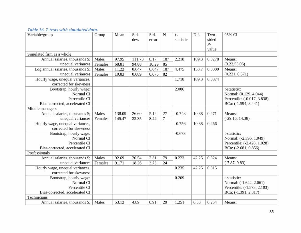
Table 16. T-tests with simulated data. Variable/group Group Mean Std.

dev. Std. error

N 𝑡𝑡-statistic

D.f. Two-sided P-value

95% CI

Simulated firm as a whole Annual salaries, thousands $;

unequal variances Males 97.95 111.73 8.17 187 2.218 189.3 0.0278 Means:

(3.22,55.06) Females 68.81 94.88 10.29 85 Log annual salaries, thousands $;

unequal variances Males 11.22 0.647 0.047 187 4.475 153.7 0.0000 Means:

(0.221, 0.571) Females 10.83 0.689 0.075 82 Hourly wage, unequal variances,

corrected for skewness 1.718 189.3 0.0874

Bootstrap, hourly wage: Normal CI

Percentile CI Bias-corrected, accelerated CI

2.086 t-statistic: Normal: (0.129, 4.044) Percentile: (-0.017, 3.838) BCa: (-1.594, 3.441)

Middle managers Annual salaries, thousands $;

unequal variances Males 138.09 26.60 5.12 27 -0.748 10.88 0.471 Means:

(-29.16, 14.38) Females 145.47 22.35 8.44 7 Hourly wage, unequal variances,

corrected for skewness -0.756 10.88 0.466

Bootstrap, hourly wage: Normal CI

Percentile CI Bias-corrected, accelerated CI

-0.673 t-statistic: Normal: (-2.396, 1.049) Percentile: (-2.428, 1.028) BCa: (-2.681, 0.856)

Professionals Annual salaries, thousands $;

unequal variances Males 92.69 20.54 2.31 79 0.223 42.25 0.824 Means:

(-7.87, 9.83) Females 91.71 18.26 3.73 24 Hourly wage, unequal variances,

corrected for skewness 0.235 42.25 0.815

Bootstrap, hourly wage: Normal CI

Percentile CI Bias-corrected, accelerated CI

0.209 t-statistic: Normal: (-1.642, 2.061) Percentile: (-1.573, 2.103) BCa: (-1.391, 2.317)

Technicians Annual salaries, thousands $; Males 53.12 4.89 0.91 29 1.251 6.53 0.254 Means:

85

unequal variances Females 49.93 5.85 2.39 6 (-2.93, 9.32) Hourly wage, unequal variances,

corrected for skewness 1.297 6.53 0.240

Bootstrap, hourly wage: Normal CI

Percentile CI Bias-corrected, accelerated CI

1.410 t-statistic: Normal: (-0.777, 3.597) Percentile: (-0.567, 3.812) BCa: (-0.569, 3.795)

Operators Annual salaries, thousands $;

unequal variances Males 32.86 7.77 1.49 27 1.614 55.91 0.112 Means:

(-0.84, 7.77) Females 29.39 8.59 1.54 31 Hourly wage, unequal variances,

corrected for skewness 1.523 55.91 0.133

Bootstrap, hourly wage: Normal CI

Percentile CI Bias-corrected, accelerated CI

1.603 t-statistic: Normal: (-0.905, 4.112) Percentile: (-0.249, 4.571) BCa: (-1.063, 3.842)

86

Distribution comparisons Table 17 presents comparisons of distributions of wages by nonparametric Kolmogorov-Smirnov, Kruskal-Wallis and Wilcoxon tests. Although the Kolmogorov-Smirnov and Wilcoxon tests are two-sample comparison tests and therefore applicable only to the analysis of the differences between a majority group and a compound minority (white compared with nonwhite, or male compared with female), the Kruskal-Wallis test is applicable for comparisons in which multiple groups are involved (such as race/ethnicity). The p-values of Wilcoxon test are based on asymptotic approximation with the exact first two moments of the test statistic distribution. For the establishment as a whole, the tests strongly reject the null hypothesis of equality. However, more detailed analysis within subgroups shows absence of differences by gender. These tests replicate the findings of the overall t-test, producing a strong rejection of equality of distributions. Once again, this is not surprising given the distributions plotted in Figure 9.

Table 17. Nonparametric distribution comparison tests for simulated data. Factor Kolmogorov-

Smirnov p-value Kruskal-Wallis p-value

Wilcoxon p-value Wilcoxon test stratified by job group, p-value

Gender 0.000 0.000 0.000 0.064 Race/ethnicity N/A 0.022 Gender by race/ethnicity N/A 0.000

Sensitivity analysis, reported in Table 18, was undertaken to quantify the strength of a hypothetical confounder that would be necessary to explain the observed differences between genders.187 The results in the second column suggest that, should the gender have zero effect and the differences between males and females be due only to an unobserved factor, then this factor must have the relative odds of about 2.4 of presence between the two groups to make the results insignificant. The results are moderately sensitive to the lack of the measurement of the factor responsible for differences in salaries. As a matter of fact, such a factor is the classification into job groups, as in the simulation processes the job groups rather than gender drove the difference in salaries. Table 13 shows that the odds ratios of employment in the different job groups range from a 6:1 male-to-female ratio among senior executives to a 4:10 ratio among clerks. When job groups are incorporated, the results are highly sensitive, with values of Γ=1.3 sufficient to remove significance of the finding. In other words, the significance of the original Wilcoxon test can be easily explained by incorporating job groups as a matching variable.

Table 18. Sensitivity analysis of the differences between salaries of males and females. Γ , the bound on the odds ratio of the confounder

Pooled analysis, upper bound for p-value

Matched job groups analysis, upper bound for p-value

1.0 0.0000 0.0000 1.1 0.0000 0.0000 1.2 0.0000 0.0002 1.3 0.0000 0.0547 1.4 0.0000 0.5722 1.5 0.0001 0.9673 1.6 0.0004 0.9997 1.7 0.0013 1.0000

187 Rosenbaum 2002.

87

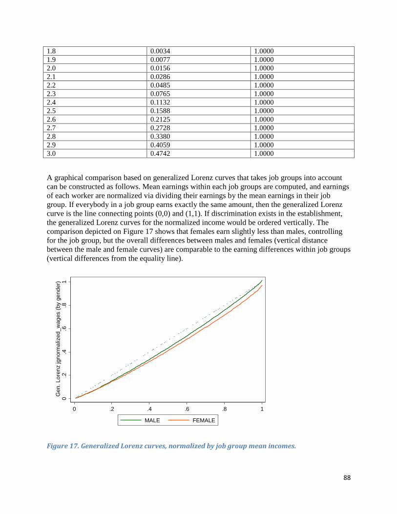
1.8 0.0034 1.0000 1.9 0.0077 1.0000 2.0 0.0156 1.0000 2.1 0.0286 1.0000 2.2 0.0485 1.0000 2.3 0.0765 1.0000 2.4 0.1132 1.0000 2.5 0.1588 1.0000 2.6 0.2125 1.0000 2.7 0.2728 1.0000 2.8 0.3380 1.0000 2.9 0.4059 1.0000 3.0 0.4742 1.0000

A graphical comparison based on generalized Lorenz curves that takes job groups into account can be constructed as follows. Mean earnings within each job groups are computed, and earnings of each worker are normalized via dividing their earnings by the mean earnings in their job group. If everybody in a job group earns exactly the same amount, then the generalized Lorenz curve is the line connecting points (0,0) and (1,1). If discrimination exists in the establishment, the generalized Lorenz curves for the normalized income would be ordered vertically. The comparison depicted on Figure 17 shows that females earn slightly less than males, controlling for the job group, but the overall differences between males and females (vertical distance between the male and female curves) are comparable to the earning differences within job groups (vertical differences from the equality line).

Figure 17. Generalized Lorenz curves, normalized by job group mean incomes.

0.2

.4.6

.81

Gen

. Lor

enz

jgno

rmal

ized

_wag

es (b

y ge

nder

)

0 .2 .4 .6 .8 1

MALE FEMALE

88

Permutation tests Permutation tests were performed on the simulated data, with results provided in Table 19. Although the within-job-group t-tests in Table 16 did not show the differences in the mean pay between genders, permutation testing found these differences within some of the job groups. Although the analysis across the whole establishment demonstrated differences in salaries between males and females, stratified permutation within job groups removed the biases due to different gender compositions of the different job groups. In the regression approach, no tangible difference existed between permutation across the whole establishment and within the job groups, because the method itself controls for the differences in salaries between the job groups.

Table 19. Permutation tests with simulated data. Analysis and statistic permuted Job groups Permutation by… p-value Total, males Establishment as a whole Outcome (annual salary) 0.011 Total, males Establishment as a whole Outcome (annual salary)

within job groups 0.708

Total, males Middle managers Outcome (annual salary) 0.018 Total, males Professionals Outcome (annual salary) 0.365 Total, males Technicians Outcome (annual salary) 0.999 Total, males Operators Outcome (annual salary) 1.000 ANOVA (annual salary on gender), F-statistic

Establishment as a whole Demographic variable (gender)

0.031

ANOVA (annual salary on gender), F-statistic

Establishment as a whole Demographic variable (gender) within job groups

0.723

ANOVA (annual salary on race), F-statistic

Establishment as a whole Demographic variable (race)

0.182

ANOVA (annual salary on race), F-statistic

Establishment as a whole Demographic variable (race) within job groups

0.815

Regression (control + design specification), F-statistic of the Wald test for gender

Establishment as a whole Demographic variables (gender and race)

0.153

Regression (control + design specification), F-statistic of the Wald test for gender

Establishment as a whole Demographic variables (gender and race) within job groups

0.152

Regression (control + design specification), F-statistic of the Wald test for race

Establishment as a whole Demographic variables (gender and race)

0.490

Regression (control + design specification), F-statistic of the Wald test for race

Establishment as a whole Demographic variables (gender and race) within job groups

0.464

Visualization of the permutation tests is provided in Figure 10. Simulated permutation distributions are shown as histograms, and the observed statistics as vertical lines, so that p-values are given by the area of the histogram to the right of the observed test statistic. Figure 10(a) is the permutation of gender across the whole establishment, demonstrating significant differences between males and females across it. Figure 10(b) shows conditional permutation within job groups. As the job groups drive the difference between pay levels, including them in the regression helps explaining most of the between-person variability, leaving gender insignificant. Although close to normal, both distributions are asymmetric and slightly skewed to

89

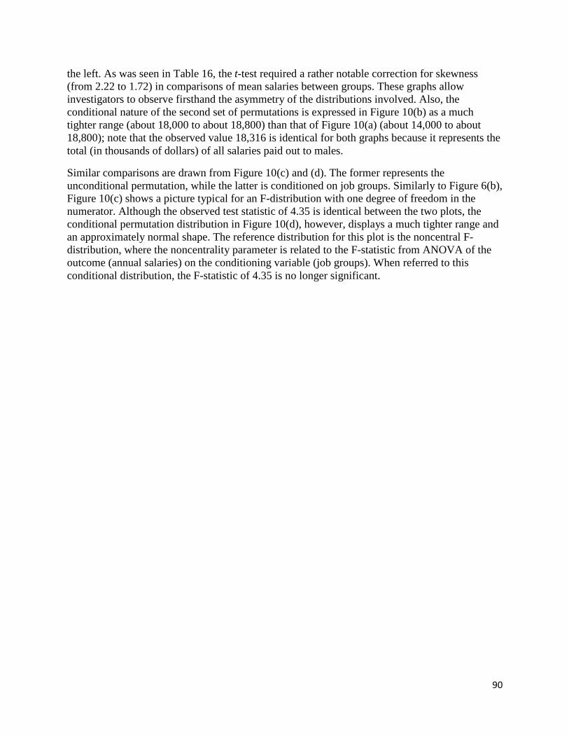
the left. As was seen in Table 16, the t-test required a rather notable correction for skewness (from 2.22 to 1.72) in comparisons of mean salaries between groups. These graphs allow investigators to observe firsthand the asymmetry of the distributions involved. Also, the conditional nature of the second set of permutations is expressed in Figure 10(b) as a much tighter range (about 18,000 to about 18,800) than that of Figure 10(a) (about 14,000 to about 18,800); note that the observed value 18,316 is identical for both graphs because it represents the total (in thousands of dollars) of all salaries paid out to males.

Similar comparisons are drawn from Figure 10(c) and (d). The former represents the unconditional permutation, while the latter is conditioned on job groups. Similarly to Figure 6(b), Figure 10(c) shows a picture typical for an F-distribution with one degree of freedom in the numerator. Although the observed test statistic of 4.35 is identical between the two plots, the conditional permutation distribution in Figure 10(d), however, displays a much tighter range and an approximately normal shape. The reference distribution for this plot is the noncentral F-distribution, where the noncentrality parameter is related to the F-statistic from ANOVA of the outcome (annual salaries) on the conditioning variable (job groups). When referred to this conditional distribution, the F-statistic of 4.35 is no longer significant.

90

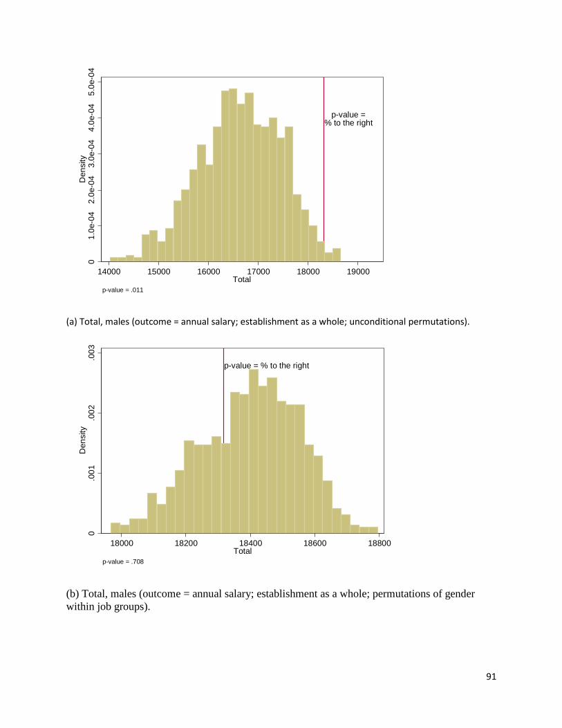
(a) Total, males (outcome = annual salary; establishment as a whole; unconditional permutations).

(b) Total, males (outcome = annual salary; establishment as a whole; permutations of gender within job groups).

p-value =% to the right

01.

0e-0

42.

0e-0

43.

0e-0

44.

0e-0

45.

0e-0

4D

ensi

ty

14000 15000 16000 17000 18000 19000Total

p-value = .011

p-value = % to the right

0.0

01.0

02.0

03D

ensi

ty

18000 18200 18400 18600 18800Total

p-value = .708

91

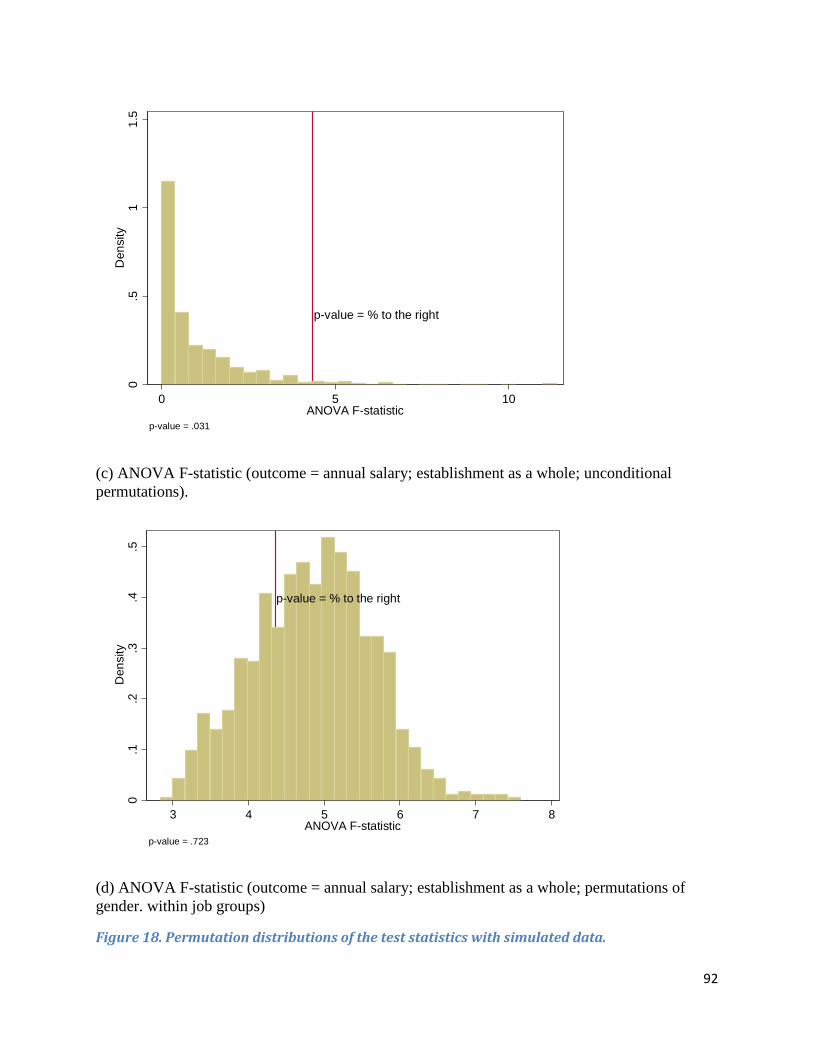
(c) ANOVA F-statistic (outcome = annual salary; establishment as a whole; unconditional permutations).

(d) ANOVA F-statistic (outcome = annual salary; establishment as a whole; permutations of gender. within job groups)

Figure 18. Permutation distributions of the test statistics with simulated data.

p-value = % to the right

0.5

11.

5D

ensi

ty

0 5 10ANOVA F-statistic

p-value = .031

p-value = % to the right

0.1

.2.3

.4.5

Den

sity

3 4 5 6 7 8ANOVA F-statistic

p-value = .723

92

Analysis of grouped salary data To illustrate the analysis of salary data organized in pay bands, the existing simulated salaries were recorded according to the categories currently used in EEO-4. The categories and distribution for this simulated firm are reported in Table 20. This tabulation shows issues with the categories: the two lowest categories are not used at all, whereas the highest salary category is overpopulated, with nearly a half of all simulated employees having salaries in the above $70,000 range.

Table 20. Distribution of salaries in the simulated firm in EEO-4 categories. EEO-4 bracket Salary range Count Percent 1 0–15.9K 0 0% 2 16K–19.9K 0 0% 3 20K–24.9K 12 4.41% 4 25K–32.9K 41 15.07% 5 33K–42.9K 25 9.19% 6 43K–54.9K 34 12.50% 7 55K–69.9K 31 11.40% 8 70K+ 129 47.43%

Since most of the implementations of the nonparametric tests expect raw data as inputs, the EEO-4 (or similar proposed) forms need to be converted into a micro data set by expanding each of the responding cells and creating the observations representing workers in the given cell. For instance, in the simulated firm, there are 10 males and 2 females in the professional job group earning $55,000 to $69,999. For these cells, 10 observations would need to be created with professional job group designation, male gender, and the value of 7 for the 7th income bracket that they fall into; and 2 observations would need to be created with professional group designation, female gender, and income rank equal to 7.

Because the salary variable in its grouped form is only an ordinal variable, most of the applicable analyses are based on ranks. As discussed previously in “Nonparametric Distribution Comparison,” the analogue of the t-test is the test of medians, with the results reported in Table 21. It shows strong differences for the company as a whole as well as for the operator subgroup. All of the salaries for middle managers are above $70,000, so no test with the salary brackets can be performed. A somewhat weaker test is the cross-tabulation with Pearson or the likelihood ratio 𝜒𝜒2 test for independence of the margins. Unlike the tests based on ranks, the cross-tabulation ignores ordering that exists between the categories of the grouped variable.

Table 21. Nonparametric tests for grouped simulated data. Group Wilcoxon rank sum

(two-sample Mann-Whitney test) Cross-tabulation

𝑧𝑧-statistic Two-sided P-value Pearson 𝜒𝜒2 (d.f.) p-value Whole establishment 4.483 0.000 41.77 (5) 0.000 Middle managers . . . . Professionals -0.287 0.774 0.480 (2) 0.787 Technicians 0.545 0.586 5.026 (2) 0.081 Operators 2.978 0.003 15.34 (2) 0.004

Permutation tests were performed for some of the test statistics listed above, conditional on job groups. The permutation p-value for the cross-tabulation of salary ranges against gender

93

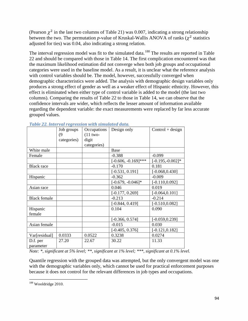
(Pearson 𝜒𝜒2 in the last two columns of Table 21) was 0.007, indicating a strong relationship between the two. The permutation p-value of Kruskal-Wallis ANOVA of ranks (𝜒𝜒2 statistics adjusted for ties) was 0.04, also indicating a strong relation.

The interval regression model was fit to the simulated data.188 The results are reported in Table 22 and should be compared with those in Table 14. The first complication encountered was that the maximum likelihood estimation did not converge when both job groups and occupational categories were used in the baseline model. As a result, it is unclear what the reference analysis with control variables should be. The model, however, successfully converged when demographic characteristics were added. The analysis with demographic design variables only produces a strong effect of gender as well as a weaker effect of Hispanic ethnicity. However, this effect is eliminated when either type of control variable is added to the model (the last two columns). Comparing the results of Table 22 to those in Table 14, we can observe that the confidence intervals are wider, which reflects the lesser amount of information available regarding the dependent variable: the exact measurements were replaced by far less accurate grouped values.

Table 22. Interval regression with simulated data. Job groups

(9 categories)

Occupations (11 two-digit categories)

Design only Control + design

White male Base Female -0.388 -0.099 [-0.606, -0.169]*** [-0.195,-0.002]* Black race -0.170 0.181 [-0.531, 0.191] [-0.068,0.430] Hispanic -0.362 -0.009 [-0.679, -0.046]* [-0.110,0.092] Asian race 0.046 0.019 [-0.177, 0.269] [-0.064,0.101] Black female -0.213 -0.214 [-0.844, 0.419] [-0.510,0.082] Hispanic female

0.104 0.090

[-0.366, 0.574] [-0.059,0.239] Asian female -0.015 0.030 [-0.405, 0.376] [-0.121,0.182] Var[residual] 0.0333 0.0522 0.3238 0.0274 D.f. per parameter

27.20 22.67 30.22 11.33

Note: *, significant at 5% level; **, significant at 1% level; ***, significant at 0.1% level.

Quantile regression with the grouped data was attempted, but the only convergent model was one with the demographic variables only, which cannot be used for practical enforcement purposes because it does not control for the relevant differences in job types and occupations.

188 Wooldridge 2010.

94

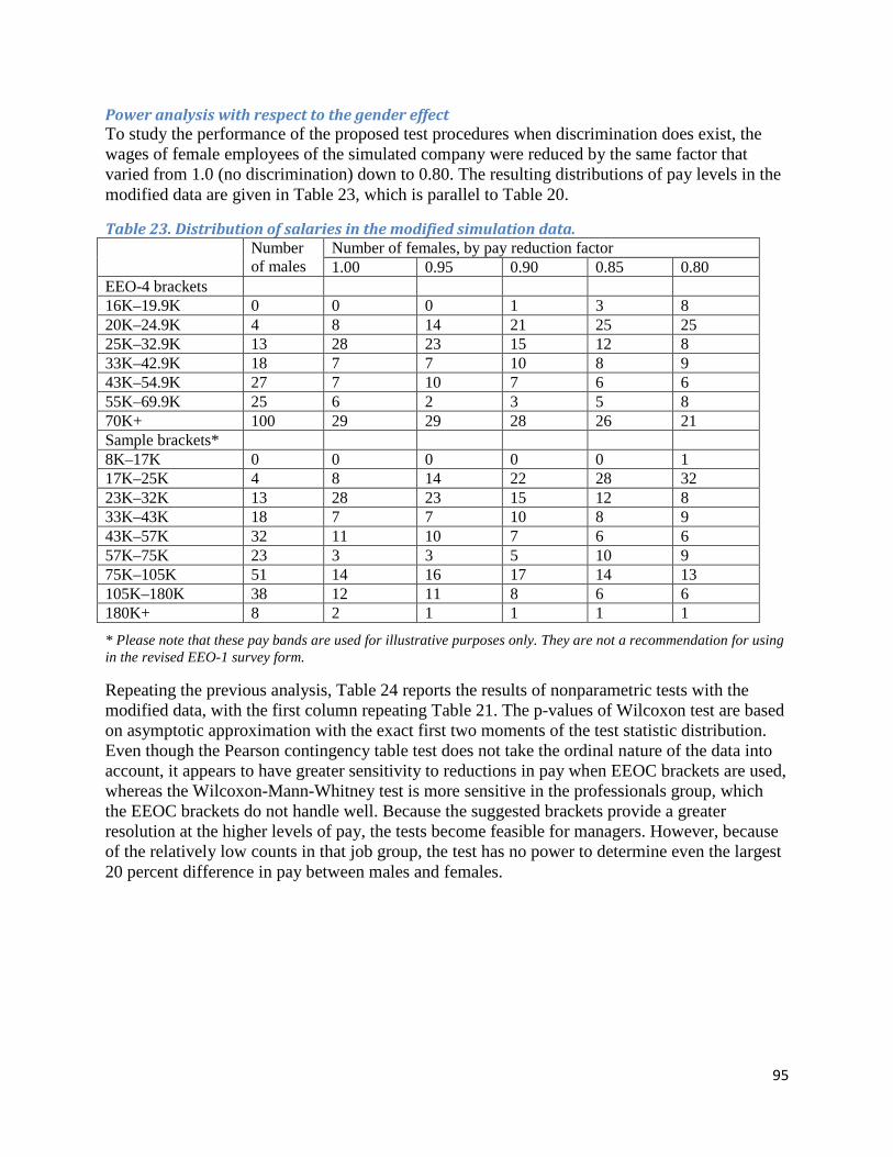
Power analysis with respect to the gender effect To study the performance of the proposed test procedures when discrimination does exist, the wages of female employees of the simulated company were reduced by the same factor that varied from 1.0 (no discrimination) down to 0.80. The resulting distributions of pay levels in the modified data are given in Table 23, which is parallel to Table 20.

Table 23. Distribution of salaries in the modified simulation data. Number

of males Number of females, by pay reduction factor 1.00 0.95 0.90 0.85 0.80

EEO-4 brackets 16K–19.9K 0 0 0 1 3 8 20K–24.9K 4 8 14 21 25 25 25K–32.9K 13 28 23 15 12 8 33K–42.9K 18 7 7 10 8 9 43K–54.9K 27 7 10 7 6 6 55K–69.9K 25 6 2 3 5 8 70K+ 100 29 29 28 26 21 Sample brackets* 8K–17K 0 0 0 0 0 1 17K–25K 4 8 14 22 28 32 23K–32K 13 28 23 15 12 8 33K–43K 18 7 7 10 8 9 43K–57K 32 11 10 7 6 6 57K–75K 23 3 3 5 10 9 75K–105K 51 14 16 17 14 13 105K–180K 38 12 11 8 6 6 180K+ 8 2 1 1 1 1

* Please note that these pay bands are used for illustrative purposes only. They are not a recommendation for using in the revised EEO-1 survey form.

Repeating the previous analysis, Table 24 reports the results of nonparametric tests with the modified data, with the first column repeating Table 21. The p-values of Wilcoxon test are based on asymptotic approximation with the exact first two moments of the test statistic distribution. Even though the Pearson contingency table test does not take the ordinal nature of the data into account, it appears to have greater sensitivity to reductions in pay when EEOC brackets are used, whereas the Wilcoxon-Mann-Whitney test is more sensitive in the professionals group, which the EEOC brackets do not handle well. Because the suggested brackets provide a greater resolution at the higher levels of pay, the tests become feasible for managers. However, because of the relatively low counts in that job group, the test has no power to determine even the largest 20 percent difference in pay between males and females.

95

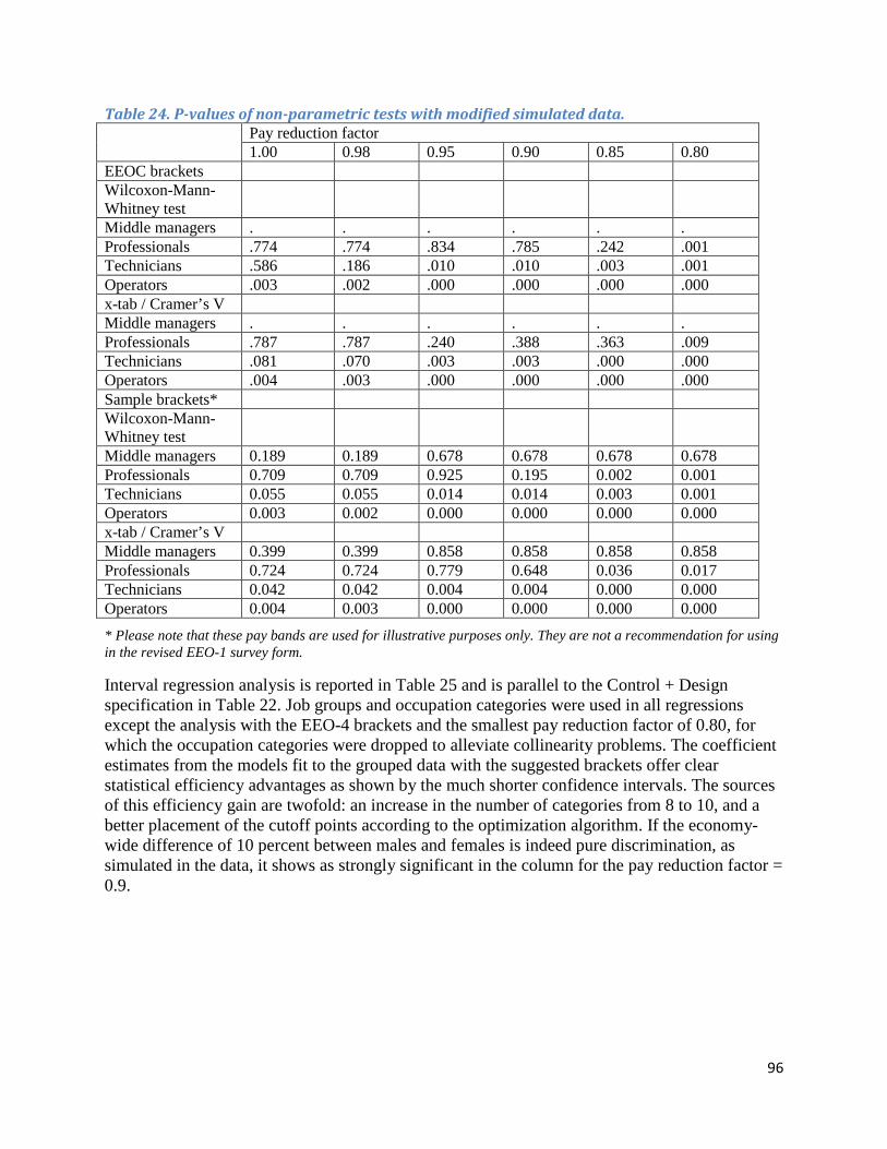
Table 24. P-values of non-parametric tests with modified simulated data. Pay reduction factor

1.00 0.98 0.95 0.90 0.85 0.80 EEOC brackets Wilcoxon-Mann-Whitney test

Middle managers . . . . . . Professionals .774 .774 .834 .785 .242 .001 Technicians .586 .186 .010 .010 .003 .001 Operators .003 .002 .000 .000 .000 .000 x-tab / Cramer’s V Middle managers . . . . . . Professionals .787 .787 .240 .388 .363 .009 Technicians .081 .070 .003 .003 .000 .000 Operators .004 .003 .000 .000 .000 .000 Sample brackets* Wilcoxon-Mann-Whitney test

Middle managers 0.189 0.189 0.678 0.678 0.678 0.678 Professionals 0.709 0.709 0.925 0.195 0.002 0.001 Technicians 0.055 0.055 0.014 0.014 0.003 0.001 Operators 0.003 0.002 0.000 0.000 0.000 0.000 x-tab / Cramer’s V Middle managers 0.399 0.399 0.858 0.858 0.858 0.858 Professionals 0.724 0.724 0.779 0.648 0.036 0.017 Technicians 0.042 0.042 0.004 0.004 0.000 0.000 Operators 0.004 0.003 0.000 0.000 0.000 0.000 * Please note that these pay bands are used for illustrative purposes only. They are not a recommendation for using in the revised EEO-1 survey form.

Interval regression analysis is reported in Table 25 and is parallel to the Control + Design specification in Table 22. Job groups and occupation categories were used in all regressions except the analysis with the EEO-4 brackets and the smallest pay reduction factor of 0.80, for which the occupation categories were dropped to alleviate collinearity problems. The coefficient estimates from the models fit to the grouped data with the suggested brackets offer clear statistical efficiency advantages as shown by the much shorter confidence intervals. The sources of this efficiency gain are twofold: an increase in the number of categories from 8 to 10, and a better placement of the cutoff points according to the optimization algorithm. If the economy-wide difference of 10 percent between males and females is indeed pure discrimination, as simulated in the data, it shows as strongly significant in the column for the pay reduction factor = 0.9.

96

Table 25. Interval regression analysis with modified simulated data. Pay reduction factor

1.00 0.98 0.95 0.90 0.85 0.80 EEO-4 brackets

White male Base Base Base Base Base Base Female -0.099 -0.112 -0.151 -0.244 -0.435 -0.621 [-0.195, -

0.002]* [-0.207, -0.017]*

[-0.251, -0.050]**

[-0.340, -0.148]***

[-0.526, -0.344]***

[-0.709, -0.533]***

Black race 0.181 0.178 0.179 0.184 0.182 0.198 [-0.068,

0.430] [-0.068, 0.424]

[-0.066, 0.423]

[-0.062, 0.431]

[-0.065, 0.429]

[-0.046, 0.442]

Hispanic -0.009 -0.014 -0.013 -0.004 -0.011 0.024 [-0.110,

0.092] [-0.116, 0.087]

[-0.117, 0.092]

[-0.105, 0.096]

[-0.112, 0.090]

[-0.076, 0.125]

Asian race 0.019 0.014 0.013 0.012 0.012 0.002 [-0.064,

0.101] [-0.069, 0.097]

[-0.071, 0.098]

[-0.074, 0.098]

[-0.073, 0.097]

[-0.097, 0.102]

Black female -0.214 -0.206 -0.177 -0.230 -0.185 -0.335 [-0.510,

0.082] [-0.500, 0.087]

[-0.467, 0.114]

[-0.496, 0.035]

[-0.471, 0.102]

[-0.639, -0.031]*

Hispanic female

0.090 0.046 0.059 0.074 0.048 -0.056

[-0.059, 0.239]

[-0.107, 0.200]

[-0.094, 0.212]

[-0.083, 0.232]

[-0.101, 0.198]

[-0.210, 0.099]

Asian female 0.030 0.043 -0.035 0.009 0.009 -0.060 [-0.121,

0.182] [-0.108, 0.194]

[-0.192, 0.121]

[-0.139, 0.157]

[-0.139, 0.157]

[-0.229, 0.109]

D.f. per parameter

11.33 11.83 11.33 11.83 11.83 16.00†

Var[residual] 0.0274 0.0276 0.0296 0.0306 0.0312 0.0397 Proposed brackets

White male Base Base Base Base Base Base Female -0.067 -0.076 -0.106 -0.179 -0.365 -0.695 [-0.137,

0.002] [-0.146, -0.007]*

[-0.181, -0.030]**

[-0.262, -0.097]***

[-0.466, -0.263]***

[-0.837, -0.552]***

Black race 0.134 0.132 0.133 0.141 0.153 0.192 [-0.054,

0.321] [-0.054, 0.318]

[-0.055, 0.321]

[-0.054, 0.336]

[-0.063, 0.369]

[-0.076, 0.460]

Hispanic -0.004 -0.008 -0.001 0.012 0.029 0.070 [-0.082,

0.074] [-0.086, 0.070]

[-0.080, 0.079]

[-0.064, 0.088]

[-0.051, 0.109]

[-0.032, 0.173]

Asian race 0.013 0.010 0.010 0.010 0.013 0.016 [-0.037,

0.064] [-0.040, 0.061]

[-0.040, 0.061]

[-0.042, 0.062]

[-0.042, 0.068]

[-0.052, 0.084]

Black female -0.197 -0.193 -0.168 -0.257 -0.300 -0.546 [-0.448,

0.055] [-0.444, 0.058]

[-0.420, 0.084]

[-0.483, -0.030]*

[-0.637, 0.038]

[-1.065, -0.027]*

97

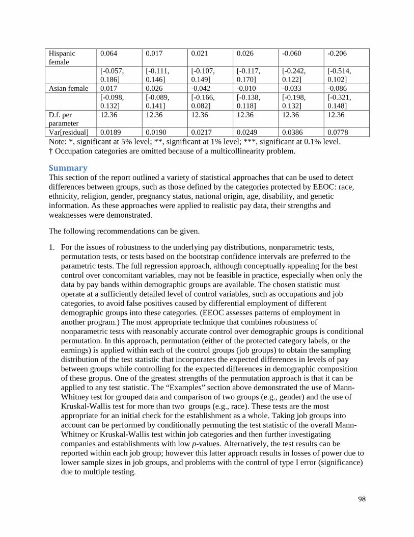
Hispanic female

0.064 0.017 0.021 0.026 -0.060 -0.206

[-0.057, 0.186]

[-0.111, 0.146]

[-0.107, 0.149]

[-0.117, 0.170]

[-0.242, 0.122]

[-0.514, 0.102]

Asian female 0.017 0.026 -0.042 -0.010 -0.033 -0.086 [-0.098,

0.132] [-0.089, 0.141]

[-0.166, 0.082]

[-0.138, 0.118]

[-0.198, 0.132]

[-0.321, 0.148]

D.f. per parameter

12.36 12.36 12.36 12.36 12.36 12.36

Var[residual] 0.0189 0.0190 0.0217 0.0249 0.0386 0.0778 Note: *, significant at 5% level; **, significant at 1% level; ***, significant at 0.1% level. † Occupation categories are omitted because of a multicollinearity problem.

Summary This section of the report outlined a variety of statistical approaches that can be used to detect differences between groups, such as those defined by the categories protected by EEOC: race, ethnicity, religion, gender, pregnancy status, national origin, age, disability, and genetic information. As these approaches were applied to realistic pay data, their strengths and weaknesses were demonstrated.

The following recommendations can be given.

1. For the issues of robustness to the underlying pay distributions, nonparametric tests, permutation tests, or tests based on the bootstrap confidence intervals are preferred to the parametric tests. The full regression approach, although conceptually appealing for the best control over concomitant variables, may not be feasible in practice, especially when only the data by pay bands within demographic groups are available. The chosen statistic must operate at a sufficiently detailed level of control variables, such as occupations and job categories, to avoid false positives caused by differential employment of different demographic groups into these categories. (EEOC assesses patterns of employment in another program.) The most appropriate technique that combines robustness of nonparametric tests with reasonably accurate control over demographic groups is conditional permutation. In this approach, permutation (either of the protected category labels, or the earnings) is applied within each of the control groups (job groups) to obtain the sampling distribution of the test statistic that incorporates the expected differences in levels of pay between groups while controlling for the expected differences in demographic composition of these gropus. One of the greatest strengths of the permutation approach is that it can be applied to any test statistic. The “Examples” section above demonstrated the use of Mann-Whitney test for grouped data and comparison of two groups (e.g., gender) and the use of Kruskal-Wallis test for more than two groups (e.g., race). These tests are the most appropriate for an initial check for the establishment as a whole. Taking job groups into account can be performed by conditionally permuting the test statistic of the overall Mann-Whitney or Kruskal-Wallis test within job categories and then further investigating companies and establishments with low p-values. Alternatively, the test results can be reported within each job group; however this latter approach results in losses of power due to lower sample sizes in job groups, and problems with the control of type I error (significance) due to multiple testing.

98

2. The issue of calibrating the error rates (power versus significance level) needs to be addressed ethically, in a way that balances the operational costs of detecting discrimination with the need to avoid false positives. Setting higher significance levels would improve the detection of discrimination but would also increase the number of false positives, leading to unnecessary investigations and eventually increasing operational costs of EEOC enforcement programs. Looking into the error rates across the sizes of companies may also be necessary, because for a given effect size, larger companies will be more likely to come under scrutiny. A three-way balancing of the effect sizes, significance levels, and power of the chosen test will be required to fine-tune the procedure in a way that is compatible with the mission of EEOC while keeping the whole operation manageable.

3. Operationally, a dashboard can be created that would relate the nominal results of statistical tests (that is, test statistics or their p-values) to those encountered in the location and the industry. On such a dashboard, the EEOC investigator would see technical information such as the values of the main statistics used to describe the establishment, and its relation to the same statistic encountered in other establishments, which could report statistics of interest as shown in Figure 11.

4. Because pay data are to be collected by salary brackets and hours worked, the pay bands would need to be carefully designed to balance usefulness of data with response burden. The brackets that EEO-4 currently uses may not be appropriate given that pay structure and levels in the economy as a whole are different from those in state and local governments. It is recommended that EEOC follow the methodology followed by OES (and outlined in earlier sections) to establish appropriate salary brackets. The number of salary brackets can also be reconsidered to balance the usability of the data and the response burden. A greater number of brackets (for example, 10 or 12 compared with the 8 salary ranges in the current EEO-4 instrument) will provide more accurate data that would correspondingly allow more detailed analysis. However, the collection of these more detailed data will proportionately increase the response burden. Producing optimal brackets remains a computational challenge. This report only provides a partial solution based on a small subsample of the existing rich CPS data.

99

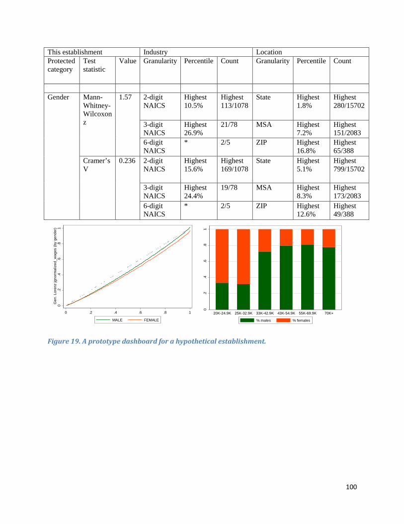
This establishment Industry Location Protected category

Test statistic

Value Granularity Percentile Count Granularity Percentile Count

Gender Mann-

Whitney-Wilcoxon z

1.57 2-digit NAICS

Highest 10.5%

Highest 113/1078

State Highest 1.8%

Highest 280/15702

3-digit NAICS

Highest 26.9%

21/78 MSA Highest 7.2%

Highest 151/2083

6-digit NAICS

* 2/5 ZIP Highest 16.8%

Highest 65/388

Cramer’s V

0.236 2-digit NAICS

Highest 15.6%

Highest 169/1078

State Highest 5.1%

Highest 799/15702

3-digit NAICS

Highest 24.4%

19/78 MSA Highest 8.3%

Highest 173/2083

6-digit NAICS

* 2/5 ZIP Highest 12.6%

Highest 49/388

Figure 19. A prototype dashboard for a hypothetical establishment.

0.2

.4.6

.81

Gen

. Lor

enz

jgno

rmal

ized

_wag

es (b

y ge

nder

)

0 .2 .4 .6 .8 1

MALE FEMALE

0.2

.4.6

.81

20K-24.9K 25K-32.9K 33K-42.9K 43K-54.9K 55K-69.9K 70K+

% males % females

100

Section III: Burden Cost Estimates for EEOC and Its Respondents This section of the report addresses the burden costs for EEOC and its respondents if compensation data were collected.

Burden Costs for EEOC With the collection of compensation data, EEOC will experience increased demands on both its information technology (IT) infrastructure and the ORIP staff who process the surveys. These one-time and ongoing burden costs are presented in this section. Costs were estimated by talking to both the survey group at EEOC and the staff responsible for the information technology (IT) infrastructure. Burden cost estimates include estimated costs for developing and implementing the systems for collecting compensation data, the hardware costs, the security concerns, and time for ORIP staff to develop the business logic for the data validation and edit checks. Both one-time and ongoing costs were estimated. For one-time costs, the charges were further divided into two categories: costs for developing the system and time spent in writing the SAS program and developing edit checks.

One-Time Costs If EEOC were to proceed to collect compensation data from employers, the online systems for EEO-1, EEO-4, and EEO-5 would need to be modified to enable this data collection. It is expected that there would be a one-time increase on the workload of ORIP staff to develop the logic and validation checks that need to be included in the online system before the report can be certified. In addition, there would be a burden on the survey staff to develop the SAS programs to validate and verify the data. One-time costs were estimated for developing the three systems and a second estimate was prepared for the increase in labor hours for data edits, validation, and analysis.

Estimated One-Time Costs for Developing Online Systems The specific tasks included in estimating system development costs are:

• Time spent to develop the logic to verify the data’s accuracy; • Programming and testing the online systems to collect compensation data; and • Hardware upgrades necessary

The following Table 26 shows the estimated one-time cost of developing the three EEOC applications to collect compensation data. To estimate some of these costs, mean hourly wages for staff anticipated to work on the development and security administration side were collected from BLS’ yearly OES for the 2014 reporting year.189 Hourly estimations were compiled by speaking with subject-matter experts about the respective job functions, using standard project management methods for burden estimation, using the program evaluation and review technique, and referencing experts in the field of project management.190,191

189 U.S. Bureau of Labor Statistics. n.d. “May 2014 National Occupational Employment and Wage Estimates: United States.” Available at http://www.bls.gov/oes/current/oes_nat.htm. 190 Ahmed, S. 2011. “How Long Does Software Development Really Take?” Project Management in Practice (blog), 18 March. Available at http://prince2msp.com/2011/03/18/how-long-does-software-development-really-take/.

101

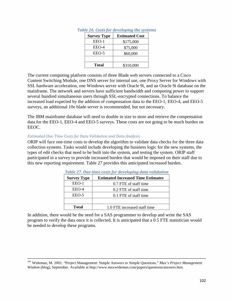
Table 26. Costs for developing the systems Survey Type Estimated Cost

EEO-1 $175,000 EEO-4 $75,000 EEO-5 $60,000

Total $310,000

The current computing platform consists of three Blade web servers connected to a Cisco Content Switching Module, one DNS server for internal use, one Proxy Server for Windows with SSL hardware acceleration, one Windows server with Oracle 9i, and an Oracle 9i database on the mainframe. The network and servers have sufficient bandwidth and computing power to support several hundred simultaneous users through SSL-encrypted connections. To balance the increased load expected by the addition of compensation data to the EEO-1, EEO-4, and EEO-5 surveys, an additional 10e blade server is recommended, but not necessary.

The IBM mainframe database will need to double in size to store and retrieve the compensation data for the EEO-1, EEO-4 and EEO-5 surveys. These costs are not going to be much burden on EEOC.

Estimated One-Time Costs for Data Validation and Data Analysis ORIP will face one-time costs to develop the algorithm to validate data checks for the three data collection systems. Tasks would include developing the business logic for the new systems, the types of edit checks that need to be built into the system, and testing the system. ORIP staff participated in a survey to provide increased burden that would be imposed on their staff due to this new reporting requirement. Table 27 provides this anticipated increased burden.

Table 27. One-time costs for developing data validation Survey Type Estimated Increased Time Estimates

EEO-1 0.7 FTE of staff time EEO-4 0.2 FTE of staff time EEO-5 0.1 FTE of staff time

Total 1.0 FTE increased staff time

In addition, there would be the need for a SAS programmer to develop and write the SAS program to verify the data once it is collected. It is anticipated that a 0.5 FTE statistician would be needed to develop these programs.

191 Wideman, M. 2001. “Project Management: Simple Answers to Simple Questions.” Max’s Project Management Wisdom (blog), September. Available at http://www.maxwideman.com/papers/questions/answers.htm.

102

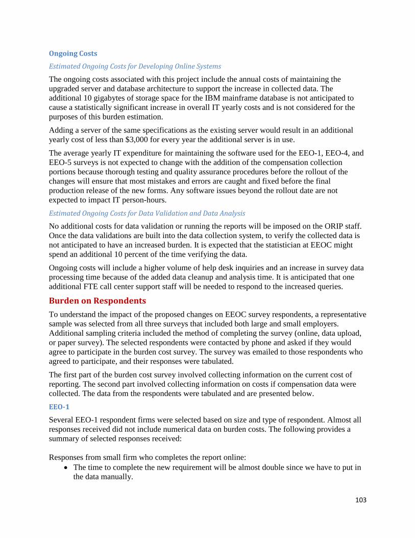
Ongoing Costs

Estimated Ongoing Costs for Developing Online Systems

The ongoing costs associated with this project include the annual costs of maintaining the upgraded server and database architecture to support the increase in collected data. The additional 10 gigabytes of storage space for the IBM mainframe database is not anticipated to cause a statistically significant increase in overall IT yearly costs and is not considered for the purposes of this burden estimation.

Adding a server of the same specifications as the existing server would result in an additional yearly cost of less than $3,000 for every year the additional server is in use.

The average yearly IT expenditure for maintaining the software used for the EEO-1, EEO-4, and EEO-5 surveys is not expected to change with the addition of the compensation collection portions because thorough testing and quality assurance procedures before the rollout of the changes will ensure that most mistakes and errors are caught and fixed before the final production release of the new forms. Any software issues beyond the rollout date are not expected to impact IT person-hours. Estimated Ongoing Costs for Data Validation and Data Analysis

No additional costs for data validation or running the reports will be imposed on the ORIP staff. Once the data validations are built into the data collection system, to verify the collected data is not anticipated to have an increased burden. It is expected that the statistician at EEOC might spend an additional 10 percent of the time verifying the data.

Ongoing costs will include a higher volume of help desk inquiries and an increase in survey data processing time because of the added data cleanup and analysis time. It is anticipated that one additional FTE call center support staff will be needed to respond to the increased queries.

Burden on Respondents To understand the impact of the proposed changes on EEOC survey respondents, a representative sample was selected from all three surveys that included both large and small employers. Additional sampling criteria included the method of completing the survey (online, data upload, or paper survey). The selected respondents were contacted by phone and asked if they would agree to participate in the burden cost survey. The survey was emailed to those respondents who agreed to participate, and their responses were tabulated.

The first part of the burden cost survey involved collecting information on the current cost of reporting. The second part involved collecting information on costs if compensation data were collected. The data from the respondents were tabulated and are presented below. EEO-1

Several EEO-1 respondent firms were selected based on size and type of respondent. Almost all responses received did not include numerical data on burden costs. The following provides a summary of selected responses received: Responses from small firm who completes the report online:

• The time to complete the new requirement will be almost double since we have to put in the data manually.

103

Responses from respondent who completes report by data upload: • There will be some one-time costs but then there should not be much impact. • I am more concerned with the time it will take for EEOC to approve the data as there is

now going to be twice the data to approve. • We will need to work with our vendor to get the new query. Don’t see it as much of a

problem as long as we know what to report and we don’t have to change dates of reporting period.

As there was no quantitative data provided, it is not possible to provide estimates on the burden. However, in February 2012, EEOC held a two-day forum on modernization of the surveys.192 Representatives from the EEO-1 respondents were also in attendance at this forum. One of the roundtable discussions was about the impact of collecting compensation data from the survey respondents. Though the forum presented the scenario of collecting mean salary data, some of the burden cost estimates are relevant. All EEO-1 respondents agreed that collecting additional race information would be cost-prohibitive since there would be a need to collect revised race definitions from all employees. However, for reporting compensation data, the average estimate increase was approximately 96 percent. The participants at the forum were unwilling to provide detailed cost estimates or provide more data on their burden costs citing confidentiality reasons.

EEO-4 Data was calculated for large filers (such as state governments) and for smaller filers such as local governments. Table 28 provides the estimated current costs and the cost for reporting compensation data. The cost estimates show a higher cost burden for larger employers or districts. For large EEO-4 respondents such as state governments, the average one-time burden cost would be $46,234 with annual costs going down to $27,202. The annual burden costs for the large employers are estimated to be a little higher than current costs. For smaller filers such as local governments, the one-time cost would be significantly less ($150) and the annual cost for reporting would remain about the same.

Table 28. Burden costs for EEO-4 respondents

EEO-4 Respondent Size Current Costs for Reporting

Anticipated Cost for Reporting Compensation One-time

Cost Annual Cost

Large jurisdictions $21,217 $46,234 $27,202 Small jurisdictions $428 $150 $426

Please note that one large EEO-4 respondent was removed from the analysis. This respondent reported a significant decrease in the annual recurring costs for reporting compensation data. When asked for an explanation, it was explained that they were currently reporting data by entering it manually in the online system. However, they planned to upload all the data starting with the next survey cycle, which would significantly reduce their burden. Since this respondent was changing method of reporting, irrespective of the change in reporting requirements, the respondent’s responses were removed from the final analysis.

192 Unpublished report from February 2012 Forum to Modernize EEO Data Collection.

104

EEO-5 EEO-5 respondents were sampled by the method of filing their report. There were not enough responses received from EEO-5 respondents who file their report via data upload. However, of the small number who reported, they did not anticipate any significant recurring costs. They were also not able to report the one-time cost to prepare to meet this new requirement. For employers that use the online form, the average one-time burden cost would be $5,483. They expect the annual recurring cost to increase by approximately 30 percent from $1,146 to $1,484.

105

Section IV: System Enhancements The EEO-1, EEO-5, and EEO-4 are online data collection systems that allow respondents to submit data via an online form, upload data, and give directions on how to submit paper reports.

The current survey systems use Oracle database on the back end. EEO-4 and EEO-5 use J2EE Spring framework while EEO-1 is mainly JSP-based. The EEO-1 application is old and has several issues. Each JSP file has its own header information and it does not use any framework/standard, and each page has its own code. This makes it a difficult system to maintain. EEO-4 and EEO-5 systems have the capability of auto validation of data uploads which allows for an efficient data transfer. Recent changes to the EEO-1 system added the capability to allow respondents to test their upload data prior to submission. However, several validation processes are manual and time consuming.

A panel of experts in web technologies reviewed the existing systems to identify ways the data transfers can be modernized and improved. 193 The recommendations made were keeping in mind that adding compensation data would increase the burden on the respondents. The additional security concerns that would be raised by employers if compensation data collected were also taken into account. The volume of data collected would almost double and it is critical that the online systems be robust and efficient to meet this new demand.

A review of the existing systems found that EEO-4 and EEO-5 data upload allows the respondent to view their uploaded files in “real time”. The data is validated and errors are displayed prior to submission. For EEO-1, the data is uploaded to a “test” database. Even though the respondents have the option to test their upload files and check for errors, not all validation checks are made at this point. A large number of validation and edit checks are manual and lead to delay in approval of the submitted data file. Survey respondents have to wait for EEOC support staff to approve the data. If there are errors, it takes a few weeks for EEOC to transmit this information to the respondent. It is recommended that EEO-1 system data upload functionality be updated. It should include real-time data validation and testing functionality. The respondents should be given real time access to correct and fix errors. In addition, most organizational changes that impact EEO-1 data collection are manual edits. In particular, merger and acquisition increase EEOC staff workload and slows down the data collection process. It is recommended that the steps and process for approving merger and acquisition are defined further and documented. The process should be automated to the maximum extent possible.

All three systems currently allow text and CSV file uploads. It is recommended that EEOC consider using the latest platform independent lightweight data-interchange format, JSON (JavaScript Object Notation). This is text-based format with name/value pairs. JSON has many advantages over XML and other popular technologies. For example, JSON is smaller than corresponding XML files and also faster to process. In addition, transferring data using JSON is much easier because the data is stored in arrays and records while XML stores data in trees. Both have their advantages, but data transfers are much easier when the data is stored in a structure that is familiar to object-oriented languages.

193 V. Sanku, certified Java programmer; J. Thoppil, FISMA security expert; H. Reddy, a certified database programmer; and R. Bansal, an information technology expert specifically in web-based technologies.

106

Another advantage of using JSON is that it will allow the use of web-based services such as WorkDay to transmit files directly to the EEO-1 systems reducing the burden on respondents to run programs/queries to create files compatible for data upload.

All EEOC surveys initiate the data collection process by sending a hard copy letter to respondents. The hard copy contains a link to the survey and at least the login id (starting from 2015, EEO-1 survey letters will not have the password in the letter). In order to increase security and make the process more efficient, it is recommended that email be used to send the login id and the link to the survey. Once compensation data is collected, it will be imperative to assure respondents, especially the private employers, that data collection is secure. The email method is more user friendly and secure, as compared to a physical letter. The hard copy should be sent to users who either do not have a valid email id or in instances where the registered email bounces back.

Currently minimal address validation is done for EEO-1 and other surveys. It is recommended that the organization address should be validated and a geocoded address should be stored in the database. The geocoding will enable spatial and location-based analysis of data. The geocoding will also allow map-based user interfaces and reports.

The suggested recommendations for system enhancements will make the data collection more efficient and robust and also ensure data security. The one-time burden costs on EEOC to implement these changes are balanced by the reduced annual burden on the ORIP staff to perform manual data edits and validation checks as well as reduced burden in responding to emails and phone calls.

107

Section V: Conclusions This report provides recommendations to EEOC on the most appropriate definition of pay, unit of pay, and statistical tests to analyze compensation data for the purpose of identifying pay disparities and discriminatory practices. The report looks at different measures of compensation and identifies IRS’ W-2 definition of pay as most appropriate. The W-2 definition of total income, which includes supplemental compensation components, such as production and nonproduction bonuses, offers a more comprehensive picture of earnings data and may not create a measurable burden for most respondents. The report recommends collecting aggregate W-2 compensation information for the 10 EEO-1 occupation categories into pay bands, which would allow computation of within-occupation variation, across-occupation variation, and overall variation. In addition to the compensation data, total hours worked by each group should also be collected to increase the value of the data and to account for pay differences due to variation in the number of hours worked.

The pay bands would need to be carefully designed to balance usefulness of data with response burden. Determining the number of salary brackets and upper and lower bounds of each bracket is beyond the scope of this study. For purposes of this study and to illustrate the statistical methods, data from CPS was used to create 10 income ranges. The methodology followed is described in the report. The report also outlines the steps followed for the OES survey. It is, however, recommended that EEOC undertake a study to determine the actual bounds. However, if further research is not feasible due to budget constraints, an alternative would be to use the OES survey bounds. A large majority of the EEO-1 respondents are familiar with the bounds and as described in the report, BLS follows strict methodology in keeping the bounds updated.

Sample forms for the three surveys, included in the Appendix, do not specify the bounds for the pay bands but are meant to be representative of how compensation data should be collected.

The report also looked at different methods of analyzing the data. Simulated data provided by EEOC was used to provide illustrative examples of the proposed statistical methodology of use of Mann-Whitney test for grouped data and the use of Kruskal-Wallis test. An initial check for the establishment as a whole can be performed by conditionally permuting the test statistic of the overall Kruskal-Wallis test within job categories and then further investigating companies and establishments with low p-values. To account for the fact that individuals with different pay rates may end up in the same bin if they worked a different number of hours, such as when a more highly paid individual joined or left the company in midyear, the number of hours worked will be used. The report outlines methods for incorporating it in the analysis.

The report also looks at survey design and addresses concerns of balancing power versus significance level in a way that balances the operational costs of detecting discrimination with the need to avoid false positives. Setting higher significance levels would improve the detection of discrimination but would also increase the number of false positives, leading to unnecessary investigations and eventually increasing operational costs of EEOC enforcement programs.

We recommend that a dashboard be created that would relate the nominal results of statistical tests (that is, test statistics or their p-values) to those encountered in the location and the industry. On such a dashboard, the EEOC investigator would see technical information such as the values of the main statistics used to describe the establishment, and its relation to the same statistic encountered in other establishments.

108

With the collection of compensation data, EEOC will experience one-time and ongoing burden costs. Developing the three EEOC applications to collect compensation data will be a one-time cost. ORIP will face one-time costs to develop the algorithm to validate data checks. The ongoing costs associated with this project include the annual costs of maintaining the upgraded server. Adding a server of the same specifications as the existing server would result in an additional yearly cost of less than $3,000 for every year the additional server is in use.

The burden on respondents was ascertained with the aid of a burden cost survey. A representative sample was selected from all three EEOC surveys that included both large and small employers and the survey was emailed to those respondents who agreed to participate. For EEO-1, the respondents did not provide any quantitative data, so it is not possible to provide estimates on the burden. For EEO-4, the cost estimates show a higher one-time cost burden for larger employers or districts, such as state governments, compared to smaller filers. There were not enough responses received from EEO-5 respondents who file their report via data upload. However, of the small number who reported, they did not anticipate any significant recurring costs. EEO-5 respondents who use the online form expect the annual cost to increase by approximately 30 percent from $1,146 to $1,484.

A panel of experts evaluated the current data collection systems and provided recommendations to improve the data transfer process. The current data collection systems for EEO-1, EEO-5, and EEO-4 allow respondents to submit data via an online form or upload data. It is recommended that EEOC consider using the latest platform-independent lightweight data-interchange format, JSON (JavaScript Object Notation), which has many advantages over XML and other popular technologies. Additionally, the JSP-based EEO-1 system should be re-designed using J2EE framework and the data upload functionality should be updated to include real-time data validation and testing functionality.

109

Appendix A: Background Material on Piecewise Quadratic Density Estimation

A-1

The Piecewise Quadratic Density Estimation (PQDE) method offers an alternative to using assumed mean methods for deriving reliable estimates for interval censored data. PQDE is a density estimator derived from a single histogram and is defined as “a piecemeal quadratic polynomial with adjustments made at the right and left extremes of the domain.” O’Malley notes that the PQDE method is based on the assumption that the “area in each interval of a frequency histogram is preserved” and that “the curve should be somewhat smooth with no large spikes or jumps between intervals.” These assumptions while not essential for a density estimator, allow for one that is simple and potentially well suited for large samples, such as the OES data.

OES estimates are derived from a large sample of over 1.2 million establishments. Wage information is collected in 12 non-overlapping wage rate intervals and the means and variances for the 12 intervals are calculated using point data from the National Compensation Survey (NCS). Hesley and Duff apply O’Malley’s PQDE to OES data as an alternative to the current NCS method. When using PQDE, “employment within a wage interval is represented by the area under a curve drawn to show the estimated relationship between employment and hourly wage rate within the wage interval.” Hesley and Duff start with plotting weighted proportions in each interval as a histogram of wage intervals “where the height of the histogram in each interval represents the employment in that interval.” The area in each of the intervals and the interval boundaries are used to derive a quadratic equation to represent the relationship between wage and employment in each interval. This procedure applies only to “center intervals where adjacent histogram bars are present on the right and left.” To maintain continuity, if either adjacent interval is zero the boundary (the average of the heights of the adjacent histogram bars) values are set to zero.

When intervals with small proportion of employment are in between or adjacent to intervals with very large proportion of employment, it is possible for parabolas in those intervals with small proportions to fall below zero. In such a case, the parabola is “replaced by one or more lines which drop from the larger interval to zero in a way that preserves area.” To handle the end intervals in OES, where the beginning Interval A is closed bound and the uppermost Interval L is unbounded, O’Malley suggests the area under the Interval A should be represented with a linear polynomial. However, in applying the PQDE method to OES data, Hesley and Duff find that a straight line estimator is not appropriate for the lowermost Interval A. The interval is not suited for PQDE since it does not have another interval below to gather information from. Interval L is particularly difficult as there is little information regarding the location and spread of the data and this interval can have a large impact on the mean and higher percentiles. O’Malley notes that the “extent of this problem must be limited by raising the lower bound of the last interval until it is large enough that only a small tail remains in the rightmost interval.” An exponential distribution can then be used to describe the tail.

Hesley and Duff conclude that the PQDE method shows “promising results” and adequately represents intervals B through K at the national major occupation group level of data. They also note that further research is required on applying PQDE to Interval A.

An exhaustive literature search did not show any applicable examples of the PQDE method being utilized for large data samples, but this is an area that EEOC researchers can explore further, especially if the application of this method for sparse cells is possible. This type of research, however, is outside the scope of this study.

A-2

Appendix B: Sample EEO-1 Form

B-1

● Equal Employment Opportunity Commission ● Office of Federal Contract Compliance Programs (Labor)

a.b.c.◦d.

County State ZIP code

f.

City or Town State ZIP code2. Establishment for which this report is fi led (omit if same as label)a. Name of establishment

2. Is your company affi l iated through common ownership and/or centralized management with other entities in an enterprise with a total employment of 100 or more?

NOTE: If the answer is yes to questions 1, 2, or 3, complete the entire form, otherwise skip to Section G.

□ Yes □ No

□ Yes □ No

□ Yes □ No

If the response to question C-3 is yes, please enter your Dun and Bradstreet identification number (if you have one): │ │ │ │ │ │ │ │ │ │

3. Does the company or any of its establishments (a) have 50 or more employees AND (b) is not exempt as provided by 41 CFR 60-1.5, AND either (1) is a prime government contractor or first-tier subcontractor, and has a contract, subcontract, or purchase order amounting to $50,000 or more, or (2) serves as a depository of Government funds in any amount or is a financial institution which is an issuing and paying agent for U.S. Savings Bonds and Savings Notes?

1. Does the entire company have at least 1 00 employees in the payroll period for which you are reporting?

Address (Number and street) City or Town e.

b. Employer identification No. (IRS 9-DIGIT TAX NUMBER) │ │ │ │ │ │ │ │ c. Was an EEO-1 report fi led for this establishment last year? □ Yes □ No

Section C- EMPLOYERS WHO ARE REQUIRED TO FILE (To be answered by all employers)

a. Name of parent company (owns or controls establishment in item 2) omit if same as labelAddress (Number and street)

Section A-TYPE OF REPORT Refer to instructions for number and types of reports to be filed

(1) □ Single-establishment Employer Report

1. Indicate by marking in the appropriate box the type of reporting unit for which this copy of the form is submitted (MARK ONLY ONE BOX).

Multi-establishment Employer: (2) □ Consolidation Report (Required) (3) □ Headquarters Unit Report (Required) (4) □ Individual Establishment Report (submit one for each establishment with 50 or more employees) (5) □ Special Report

2. Total number of reports being fi led by this Company (Answer on Consolidated Report only) _______________

OFFICE USE ONLY

O.M.B.No.FORM APPROVAL:

EQUAL EMPLOYMENT OPPORTUNITY EMPLOYER INFORMATION REPORT EEO-1

Standard Form 100REV. MM/YYYY

Section B-COMPANY IDENTIFICATION (T o be answered by all employers) 1. Parent Company

Joint ReportingCommittee

B-1

B-2

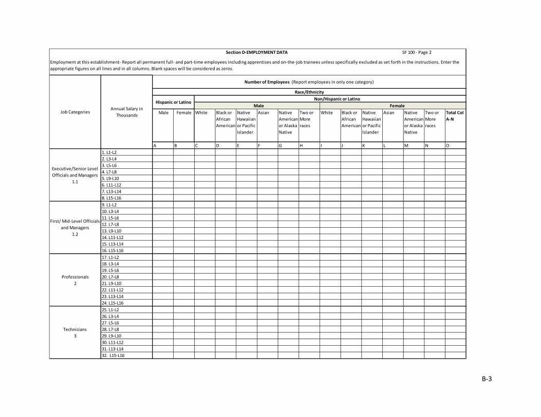
Male Female Male Female White Black or

African American

Native Hawaiian or Pacific Islander

Asian Native American or Alaska Native

Two or More races

White Black or African American

Native Hawaiian or Pacific Islander

Asian Native American or Alaska Native

Two or More races

Total Col A-N

A B C D E F G H I J K L M N O1. L1-L22. L3-L43. L5-L64. L7-L85. L9-L106. L11-L127. L13-L148. L15-L169. L1-L210. L3-L411. L5-L612. L7-L813. L9-L1014. L11-L1215. L13-L1416. L15-L1617. L1-L218. L3-L419. L5-L620. L7-L821. L9-L1022. L11-L1223. L13-L1424. L15-L1625. L1-L226. L3-L427. L5-L628. L7-L829. L9-L1030. L11-L1231. L13-L1432. L15-L16

Hispanic or Latino

Employment at this establishment- Report all permanent full- and part-time employees including apprentices and on-the-job trainees unless specifically excluded as set forth in the instructions. Enter the appropriate figures on all lines and in all columns. Blank spaces will be considered as zeros.

Number of Employees (Report employees in only one category)

Race/Ethnicity Non/Hispanic or Latino

Executive/Senior Level Officials and Managers

1.1

First/ Mid-Level Officials and Managers

1.2

Job CategoriesAnnual Salary in

Thousands

Section D-EMPLOYMENT DATA SF 100 - Page 2

Professionals 2

Technicians 3

B-3

33. L1-L234. L3-L435. L5-L636. L7-L837. L9-L1038. L11-L1239. L13-L1440. L15-L1641. L1-L242. L3-L443. L5-L644. L7-L845. L9-L1046. L11-L1247. L13-L1448. L15-L1649. L1-L250. L3-L451. L5-L652. L7-L853. L9-L1054. L11-L1255. L13-L1456. L15-L1657. L1-L258. L3-L459. L5-L660. L7-L861. L9-L1062. L11-L1263. L13-L1464. L15-L1665. L1-L266.L3-L467. L5-L668. L7-L869. L9-L1070. L11-L1271. L13-L1472. L15-L1673. L1-L274. L3-L475. L5-L676. L7-L877. L9-L1078. L11-L1279. L13-L1480. L15-L16

Total 81.PREVIOUS YEAR TOTAL 82.

Administrative Support Workers

5

Operatives 7

Laborers and Helpers 8

Service Workers 9

Sales Workers 4

Craft Workers 6

B-4

Male Female Male Female White Black or

African American

Native Hawaiian or Pacific Islander

Asian Native American or Alaska Native

Two or More races

White Black or African American

Native Hawaiian or Pacific Islander

Asian Native American or Alaska Native

Two or More races

Total Col A-N

A B C D E F G H I J K L M N O1. L1-L22. L3-L43. L5-L64. L7-L85. L9-L106. L11-L127. L13-L148. L15-L169. L1-L210. L3-L411. L5-L612. L7-L813. L9-L1014. L11-L1215. L13-L1416. L15-L1617. L1-L218. L3-L419. L5-L620. L7-L821. L9-L1022. L11-L1223. L13-L1424. L15-L1625. L1-L226. L3-L427. L5-L628. L7-L829. L9-L1030. L11-L1231. L13-L1432. L15-L16

Section D-EMPLOYMENT DATA SF 100 - Page 2

Employment at this establishment- Report all permanent full- and part-time employees including apprentices and on-the-job trainees unless specifically excluded as set forth in the instructions. Enter the appropriate figures on all lines and in all columns. Blank spaces will be considered as zeros.

Job CategoriesAnnual Salary in

Thousands

Non/Hispanic or LatinoHispanic or Latino

For each cell provide the TOTAL Number of Hours worked in last year

Executive/Senior Level Officials and

Managers 1.1

First/ Mid-Level Officials and

Managers 1.2

Professionals 2

Technicians 3

Race/Ethnicity

B-5

33. L1-L234. L3-L435. L5-L636. L7-L837. L9-L1038. L11-L1239. L13-L1440. L15-L1641. L1-L242. L3-L443. L5-L644. L7-L845. L9-L1046. L11-L1247. L13-L1448. L15-L1649. L1-L250. L3-L451. L5-L652. L7-L853. L9-L1054. L11-L1255. L13-L1456. L15-L1657. L1-L258. L3-L459. L5-L660. L7-L861. L9-L1062. L11-L1263. L13-L1464. L15-L1665. L1-L266.L3-L467. L5-L668. L7-L869. L9-L1070. L11-L1271. L13-L1472. L15-L16

Craft Workers 6

Administrative Support Workers

5

Sales Workers 4

Operatives 7

Laborers and Helpers

8

B-6

73. L1-L274. L3-L475. L5-L676. L7-L877. L9-L1078. L11-L1279. L13-L1480. L15-L16

Check 1 □one 2 □

Service Workers 9

Total 81.

Name of person to contact regarding this report

PREVIOUS YEAR TOTAL 82.

Title Address (Number and Street)

City and State Zip Code Telephone No. (including Area Code abd Extenstion Email Address

Date

1. Date(s) of payroll period used: ________________________________________________________(Omit on the Consolidate Report)

Section E -ESTABLISHMENT INFORMATION (Omit on the Consolidate Report)

All reports are accurate and were prepared in accordance with instructions. (Check on This report is accurate and was prepared in accordance with the instructions.

Name of Certifying Official Title Signature

1. What is the major activity of this establishment? (Be specific, i.e., manufacturing steel castings, retail grocer, wholesale plumbing supplies, title insurance, etc.Include the specific type of product or type of service provided, as well as the principal business or industrial activity.)

Section F- REMARKSUse this item to give any identification data appearing on the last EE0-1 report which differs from that given above, explain major changes in composition of reporting units and other pertinent information.

Section G- CERTIFICATION

B-7

Appendix C: Sample EEO-4 Form

C-1

EEOC USE ONLY

A

B

2. STREETS AND HIGHWAYS. Maintenance, repair, construction and administration of streets, alleys, sidewalks, roads, highways and bridges.

10. COMMUNITY DEVELOPMENT. Planning, zoning, land development, open space, beautification, preservation.

3. PUBLIC WELFARE. Maintenance of homes andother institutions for the needy; administration ofpublic assistance. (Hospitals and sanatoriums should be reported as item7.)

11. CORRECTIONS. Jails, reformatories, detention homes, halfway houses, prisons, parole and probation activities.

1.Financial Administration. Tax billing andcollection, budgeting, purchasing, centralaccounting and similar financial administrationcarried on by a treasurer's, auditor's orcomptroller's office andGENERAL CONTROL. Duties usually performed byboards of supervisors or commissioners, centraladministration offices and agencies, centralpersonnel or planning agencies, all judicial officesand employees (judges, magistrates, bailiffs, etc.)

9. HOUSING. Code enforcement, low rent public housing, fair housing ordinance enforcement, housing for elderly, housing rehabilitation, rent control.

A. TYPE OF GOVERNMENT (Check one box only)

□ 1. State □ 2. County □ 3. City □ 4. Township □ 5. Special District □ 6. Other (Specify)______________________________________________________________________________

B. IDENTIFICATION 1. NAME OF POLITICAL JURISDICTION (If same as label, skip to Item C)

8. HEALTH. Provision of public health services, outpatient clinics, visiting nurses, food and sanitary inspections, mental health, alcohol rehabilitation service, etc.

State/ZIPCountyCity/Town2. Address--Number and Street

C. FUNCTION

(Check one box to indicate the function(s) for which this form is being submitted. Data should be reported for all departments and agencies in your government covered by the function(s) indicated. If you cannot supply the data for every agency within the function(s) attach a list showing name and address of agencies whose data are not included.)

EQUAL EMPLOYMENT OPPORTUNITY COMMISSIONSTATE AND LOCAL GOVERNMENT INFORMATION (EEO-4)

EXCLUDE SCHOOL SYSTEMS AND EDUCATIONAL INSTITUTIONS(Read attached instructions prior to completing this form)

APPROVED BY OMB 3046-0008

EXPIRES 5/31/2018MAIL COMPLETED

FORM TO: EEO-4 Reporting CenterPO Box 8127 Reston VA 20195

DO NOT ALTER INFORMATION PRINTED IN THIS BOX

C-2

15. OTHER (Specify on Page Four)

7. HOSPITALS AND SANATORIUMS. Operation andmaintenance of institutions for inpatient medical care.

13. SANITATION AND SEWAGE. Street cleaning, garbage and refuse collection and disposal. Provision, maintenance and operation of sanitary and storm sewer systems and sewage disposal plants.

5. FIRE PROTECTION. Duties of the uniformed fireforce and clerical employees. (Report any forest fire protection activities as item 6.)

6. NATURAL RESOURCES. Agriculture, forestry, forestfire protection, irrigation drainage, flood control, etc., andPARKS AND RECREATION. Provision, maintenanceand operation of parks, playgrounds, swimming pools, auditoriums, museums, marinas, zoos, etc.

14. EMPLOYMENT SECURITY STATEGOVERNMENTS ONLY

12. UTILITIES AND TRANSPORTATION. Includes water supply, electric power, transit, gas, airports, water transportation and terminals.

4. POLICE PROTECTION. Duties of a policedepartment sheriff's, constable's, coroner's office, etc., including technical and clerical employees engaged in police activities.

C-3

Male Female

Male Female White

Black or African American Asian

Native Hawaiian or Other Pacific Islander

American Indian or Alaska Native

Two or More races White

Black or African American Asian

Native Hawaiian or Other Pacific Islander

American Indian or Alaska Native

Two or More races Total Col A-N

A B C D E F G H I J K L M N O

1. $0.1-15.92. 16.0-19.93. 20.0-24.94. 25.0-32.95. 33.0-42.96. 43.0-54.97. 55.0-69.98. 70.0 PLUS9. $0.1-15.9 10. 16.0-19.9 11. 20.0-24.9 12. 25.0-32.9 13. 33.0-42.9 14. 43.0-54.9 15. 55.0-69.9 16. 70.0 PLUS17. $0.1-15.9 18. 16.0-19.9 19. 20.0-24.9 20. 25.0-32.9 21. 33.0-42.9 22. 43.0-54.9 23. 55.0-69.9 24. 70.0 PLUS

25. $0.1-15.9 26. 16.0-19.9 27. 20.0-24.9 28. 25.0-32.9 29. 33.0-42.9 30. 43.0-54.9 31. 55.0-69.9 32. 70.0 PLUS

33. $0.1-15.9 34. 16.0-19.9 35. 20.0-24.9 36. 25.0-32.9 37. 33.0-42.9 38. 43.0-54.9 39. 55.0-69.9 40. 70.0 PLUS

41. $0.1-15.9 42. 16.0-19.9 43. 20.0-24.9 44. 25.0-32.9 45. 33.0-42.9 46. 43.0-54.9 47. 55.0-69.9 48. 70.0 PLUS

Administrative Support

Annual Salary (in thousands

000)Job Categories

D. EMPLOYMENT DATA AS OF JUNE 30 (Do not include elected/appointed officials. Blanks will be counted as zero) 1. FULLTIME EMPLOYEES (Temporary employees are not included)

Hispanic or LatinoRace/Ethnicity

Non/Hispanic or Latino

Officials Administrators

Professionals

Technicians

Protective Service

Para-Professionals

C-4

Male Female

Male Female White

Black or African American As ian

Native Hawai ian or Other Paci fic Is lander

American Indian or Alaska Native

Two or More races White

Black or African American As ian

Native Hawai ian or Other Paci fic Is lander

American Indian or Alaska Native

Two or More races

Total Col A-N

A B C D E F G H I J K L M N O49. $0.1-15.9 50. 16.0-19.9 51. 20.0-24.9 52. 25.0-32.9 53. 33.0-42.9 54. 43.0-54.9 55. 55.0-69.9 56. 70.0 PLUS57. $0.1-15.9 58. 16.0-19.9 59. 20.0-24.9 60. 25.0-32.9 61. 33.0-42.9 62. 43.0-54.9 63. 55.0-69.9 64. 70.0 PLUS

72. SKILLED CRAFT 73. SERVICE/MAINTENANCE

74. TOTAL OTHER THAN FULL TIME (LINES 66 – 73)

67. PROFESSIONALS 68. TECHNICIANS 69. PROTECTIVE SERVICE70. PARAPROFESSIONAL 71. ADMIN. SUPPORT

D. EMPLOYMENT DATA AS OF JUNE 30 (Cont.)(Do not include elected/appointed officials. Blanks will be counted as zero)

Skilled Craft

Service Maintenance

65. TOTAL FULL TIME

(LINES 1 – 64)

66. OFFICIALS/ADMIN

2. OTHER THAN FULLTIME EMPLOYEES (Including temporary employees

1. FULLTIME EMPLOYEES (Temporary employees are not included)

Categories Annual Salary (in thousands

000)

Hispanic or LatinoRace/Ethnicity

Non/Hispanic or Latino

3. NEW HIRES DURING FISCAL YEAR Permanent full time only JULY 1 – JUNE 30

75. OFFICIALS/ADMIN 76. PROFESSIONALS 77. TECHNICIANS 78. PROTECTIVE SERVICE79. PARAPROFESSIONAL 80. ADMIN. SUPPORT 81. SKILLED CRAFT 82. SERVICE/MAINTENANCE

83. TOTAL NEW HIRES (LINES 75 – 82)

C-5

Male Female

Male Female White

Black or African American As ian

Native Hawai ian or Other Paci fic Is lander

American Indian or Alaska Native

Two or More races White

Black or African American As ian

Native Hawai ian or Other Paci fic Is lander

American Indian or Alaska Native

Two or More races

Total Col A-N

A B C D E F G H I J K L M N O

1. $0.1-15.92. 16.0-19.93. 20.0-24.94. 25.0-32.9

5. 33.0-42.96. 43.0-54.97. 55.0-69.98. 70.0 PLUS9. $0.1-15.9 10. 16.0-19.9 11. 20.0-24.9

12. 25.0-32.9

13. 33.0-42.9 14. 43.0-54.9

15. 55.0-69.9

16. 70.0 PLUS

17. $0.1-15.9 18. 16.0-19.9 19. 20.0-24.9 20. 25.0-32.9

21. 33.0-42.9 22. 43.0-54.9 23. 55.0-69.9 24. 70.0 PLUS

25. $0.1-15.9 26. 16.0-19.9 27. 20.0-24.9 28. 25.0-32.9 29. 33.0-42.9 30. 43.0-54.9 31. 55.0-69.9 32. 70.0 PLUS33. $0.1-15.9 34. 16.0-19.9 35. 20.0-24.9 36. 25.0-32.9 37. 33.0-42.9 38. 43.0-54.9 39. 55.0-69.9 40. 70.0 PLUS41. $0.1-15.9 42. 16.0-19.9 43. 20.0-24.9 44. 25.0-32.9 45. 33.0-42.9 46. 43.0-54.9 47. 55.0-69.9 48. 70.0 PLUS

Administrative

Support

D. EMPLOYMENT DATA AS OF JUNE 30 (Do not include elected/appointed officials. Blanks will be counted as zero)

For each cell provide the TOTAL Number of Hours worked in last year

Job Categories

Annual Salary (in thousands

000)

Hispanic or LatinoRace/Ethnicity

Non/Hispanic or Latino

Officials Administr

ators

Professionals

Technicians

Protective Service

Para-Profession

als

C-6

Male Female

Male Female White

Black or African American As ian

Native Hawai ian or Other Paci fic Is lander

American Indian or Alaska Native

Two or More races White

Black or African American As ian

Native Hawai ian or Other Paci fic Is lander

American Indian or Alaska Native

Two or More races

Total Col A-N

A B C D E F G H I J K L M N O49. $0.1-15.9 50. 16.0-19.9 51. 20.0-24.9 52. 25.0-32.9 53. 33.0-42.9 54. 43.0-54.9 55. 55.0-69.9 56. 70.0 PLUS57. $0.1-15.9 58. 16.0-19.9 59. 20.0-24.9 60. 25.0-32.9 61. 33.0-42.9 62. 43.0-54.9 63. 55.0-69.9 64. 70.0 PLUS

Skilled Craft

Service Maintena

nce

65. TOTAL FULL TIME

D. EMPLOYMENT DATA AS OF JUNE 30 (Cont.)(Do not include elected/appointed officials. Blanks will be counted as zero)

For each cell provide the TOTAL Number of Hours worked in last year

Categories Annual Salary (in thousands

000)

Hispanic or LatinoRace/Ethnicity

Non/Hispanic or Latino

2. OTHER THAN FULLTIME EMPLOYEE Hours (Including temporary employee hours)

66. OFFICIALS/ADMIN 67. PROFESSIONALS 68. TECHNICIANS 69. PROTECTIVE SERVICE70. PARAPROFESSIONAL 71. ADMIN. SUPPORT 72. SKILLED CRAFT 73. SERVICE/MAINTENANC

74. TOTAL OTHER THAN FULL TIME (LINES 66 – 73)

3. NEW HIRES DURING FISCAL YEAR Permanent full time only JULY 1 – JUNE 30 hours

75. OFFICIALS/ADMIN 76. PROFESSIONALS 77. TECHNICIANS 78. PROTECTIVE SERVICE79. PARAPROFESSIONAL 80. ADMIN. SUPPORT 81. SKILLED CRAFT 82. SERVICE/MAINTENANC

83. TOTAL NEW HIRES (LINES 75 – 82)

C-7

YPED NAME/TITLE OF AUTHORIZED OFFICIASIGNATUREDATE

E-MAIL

NAME OF PERSON TO CONTACT REGARDING THIS FO

ADDRESS (Number and Street, City, State, Zip Code)

REMARKS (List National Crime Information Center (NCIC) number assigned to any Criminal Justice Agencies whose data are included in this report)

***LIST AGENCIES INCLUDED ON THIS FORM***

CERTIFICATION. I certify that the information given in this report is correct and true to the best of my knowledge and was reported in accordance with accompanying instructions. (Willfully false statements on this report are punishable by law, US Code, Title 18, Section

TITLE

TELEPHONE NUMBERextension: FAX NUMBER

C-8

Appendix D: Sample EEO-5 Form

D-1

EEOC FORM 168A Page 1

C. GENERAL STATISTICSNUMBER OF SCHOOLS OPERATED NUMBER OF ANNEXES OPERATED OCTOBER 1st ENROLLMENT

D. REMARK

B. SCHOOL SYSTEMS IDENTIFICATION (OMIT IS SAME AS LABEL)NAME

STREET AND NO. OR POST OFFICE BOX CITY/TOWN COUNTY STATE ZIP

Local Publ ic School Specia l Regional Agency State Education Agency Other (Speci fy)

FORM APPROVED BY OMB NO. 3046-0003

APPROVAL EXPIRES 7/31/17

EQUAL EMPLOYMENT OPPORTUNITY COMMISSION ELEMENTARY -SECONDARY STAFF INFORMATION (EEO-5)

Public school systems

This a joint requirement of the EEOC and the Office for Civi l Rights , U.S. Department of Education and the U.S. Department of Justice.

DO NOT ALTER INFORMATION PRINTED IN THIS BOX

NOTE: ALL EMPLOYEES IN YOUR SCHOOL DISTRICT MUST BE INCLUDED ON THIS FORM. Additional Copies of this form may be obta ined from the address below. Send your ful l report to:

PART I. IDENTIFICATIONA. TYPE OF AGENCY WHICH OPERATES THE REPORTING SCHOOL SYSTEM

D-2

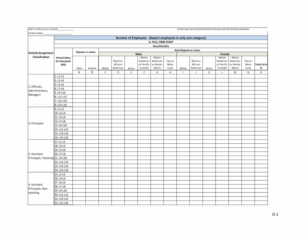
PART II. Staff Statistics of (DATE) _______________ DO NOT INCLUDE ELECTED/APPOINTED OFFICIALS (SEE DEFINITION IN APPENDIX

DISTRICT NAME:_____________________________

Male Female

Male Female White

Black or African

American Asian

Native Hawaiian or Pacific Islander

Native American or Alaska

Native

Two or More races White

Black or African

American Asian

Native Hawaiian or Pacific Islander

Native American or Alaska

Native

Two or More races

Total Col A-N

A B C D E F G H I J K L M N O

1. L1-L22. L3-L43. L5-L64. L7-L85. L9-L106. L11-L127. L13-L148. L15-L169. L1-L210. L3-L411. L5-L612. L7-L813. L9-L1014. L11-L1215. L13-L1416. L15-L1617. L1-L218. L3-L419. L5-L620. L7-L821. L9-L1022. L11-L1223. L13-L1424. L15-L1625. L1-L226. L3-L427. L5-L628. L7-L829. L9-L1030. L11-L1231. L13-L1432. L15-L16

2. Principals

3. Assistant Principals, Teaching

4. Assistant Principals, Non-teaching

1. Officials, Administrators, Managers

Race/Ethnicity

Hispanic or Latino

Number of Employees (Report employees in only one category)

Activity Assignment Classification Annual Salary

(in thousands 000)

Non/Hispanic or Latino

A. FULL-TIME STAFF

D-1

33. L1-L234. L3-L435. L5-L636. L7-L837. L9-L1038. L11-L1239. L13-L1440. L15-L1641. L1-L242. L3-L443. L5-L644. L7-L845. L9-L1046. L11-L1247. L13-L1448. L15-L1649. L1-L250. L3-L451. L5-L652. L7-L853. L9-L1054. L11-L1255. L13-L1456. L15-L1657. L1-L258. L3-L459. L5-L660. L7-L861. L9-L1062. L11-L1263. L13-L1464. L15-L1665. L1-L266.L3-L467. L5-L668. L7-L869. L9-L1070. L11-L1271. L13-L1472. L15-L1673. L1-L274. L3-L475. L5-L676. L7-L877. L9-L1078. L11-L1279. L13-L1480. L15-L16

5. Elementary Classroom Teachers

6. Secondary Classroom Teachers

7. Other Classroom Teachers

8. Guidance

9. Psychological

10. Librarians/Audiovisual Staff

D-2

81. L1-L282. L3-L483. L5-L684. L7-L885. L9-L1086. L11-L1287. L13-L1488. L15-L1689. L1-L290. L3-L491. L5-L692. L7-L893. L9-L1094. L11-L1295. L13-L1496. L15-L1697. L1-L298. L3-L499. L5-L6100. L7-L8101. L9-L10102. L11-L12103. L13-L14104. L15-L16105. L1-L2106. L3-L4107. L5-L6108. L7-L8109. L9-L10110. L11-L12111. L13-L14112. L15-L16113. L1-L2114. L3-L4115. L5-L6116. L7-L8117. L9-L10118. L11-L12119. L13-L14120. L15-L16

11. Consultants & Supervisors of Instruction

12. Other Professional Staff

13.Teacher Aides

14. Technicians

15. Administrative Support Workers

D-3

121. L1-L2122. L3-L4123. L5-L6124. L7-L8125. L9-L10126. L11-L12127. L13-L14128. L15-L16129. L1-L2130. L3-L4131. L5-L6132. L7-L8133. L9-L10134. L11-L12135. L13-L14136. L15-L16137. L1-L2138. L3-L4139. L5-L6140. L7-L8141. L9-L10142. L11-L12143. L13-L14144. L15-L16145. L1-L2146. L3-L4147. L5-L6148. L7-L8149. L9-L10150. L11-L12151. L13-L14152. L15-L16

16. Service Workers

17. Skilled Crafts

18. Laborers and Helpers

19. TOTALS (1-18)

D-4

Race/Ethnicity Non/Hispanic or Latino

Hispanic or Latino Male FemaleAnnual Salary (in thousands 000)

Male Female White

Black or African American Asian

Native Hawaiian or Pacific Islander

Native American or Alaska Native

Two or More races White

Black or African American Asian

Native Hawaiian or Pacific Islander

Native American or Alaska Native

Two or More races

Total Col A-N

153. L1-L2154. L3-L4155. L5-L6156. L7-L8157. L9-L10158. L11-L12159. L13-L14160. L15-L16161. L1-L2162. L3-L4163. L5-L6164. L7-L8165. L9-L10166. L11-L12167. L13-L14168. L15-L16169. L1-L2170. L3-L4171. L5-L6172. L7-L8173. L9-L10174. L11-L12175. L13-L14176. L15-L16

B. PART-TIME STAFF

20. Professional Instructional

Activity Assignment Classification

21. All Other

22. TOTALS (20-21)

D-5

177. L1-L2178. L3-L4179. L5-L6180. L7-L8181. L9-L10182. L11-L12183. L13-L14184. L15-L16185. L1-L2186. L3-L4187. L5-L6188. L7-L8189. L9-L10190. L11-L12191. L13-L14192. L15-L16193. L1-L2194. L3-L4195. L5-L6196. L7-L8197. L9-L10198. L11-L12199. L13-L14200. L15-L16201. L1-L2202. L3-L4203. L5-L6204. L7-L8205. L9-L10206. L11-L12207. L13-L14208. L15-L16209. L1-L2210. L3-L4211. L5-L6212. L7-L8213. L9-L10214. L11-L12215. L13-L14216. L15-L16217. L1-L2218. L3-L4219. L5-L6220. L7-L8221. L9-L10222. L11-L12223. L13-L14224. L15-L16

23. Officials, Administrators,

Managers

C. NEW HIRES FULL-TIME (JULY THRU SEPT. OF THE SURVEY YEAR)

24. Principals/ Assistant Principals

25. Classroom Teachers

26. Other Professional Staff

27. Nonprofessional Staff

28. TOTALS (23-27)

D-6

PART III. Staff Statistics of (DATE) _______________ DO NOT INCLUDE ELECTED/APPOINTED OFFICIALS (SEE DEFINITION IN APPENDIX

DISTRICT NAME:_____________________________

Male Female

Male Female White

Black or African American Asian

Native Hawaiian or Pacific Islander

Native American or Alaska Native

Two or More races White

Black or African American Asian

Native Hawaiian or Pacific Islander

Native American or Alaska Native

Two or More races Total Col A-N

A B C D E F G H I J K L M N O

1. L1-L22. L3-L43. L5-L64. L7-L85. L9-L106. L11-L127. L13-L148. L15-L16

9. L1-L210. L3-L411. L5-L612. L7-L813. L9-L1014. L11-L1215. L13-L1416. L15-L1617. L1-L218. L3-L419. L5-L620. L7-L821. L9-L1022. L11-L1223. L13-L1424. L15-L1625. L1-L226. L3-L427. L5-L628. L7-L829. L9-L1030. L11-L1231. L13-L1432. L15-L16

For each cell provide the TOTAL Number of Hours worked in last year A. FULL-TIME STAFF

4. Assistant Principals, Non-teaching

1. Officials, Administrators, Managers

2. Principals

3. Assistant Principals, Teaching

Hispanic or Latino

Race/Ethnicity Non/Hispanic or Latino

Activity Assignment Classification

Salary (in thousands

000)

D-7

33. L1-L234. L3-L435. L5-L636. L7-L837. L9-L1038. L11-L1239. L13-L1440. L15-L1641. L1-L242. L3-L443. L5-L644. L7-L845. L9-L1046. L11-L1247. L13-L1448. L15-L1649. L1-L250. L3-L451. L5-L652. L7-L853. L9-L1054. L11-L1255. L13-L1456. L15-L1657. L1-L258. L3-L459. L5-L660. L7-L861. L9-L1062. L11-L1263. L13-L1464. L15-L1665. L1-L266.L3-L467. L5-L668. L7-L869. L9-L1070. L11-L1271. L13-L1472. L15-L1673. L1-L274. L3-L475. L5-L676. L7-L877. L9-L1078. L11-L1279. L13-L1480. L15-L16

5. Elementary Classroom Teachers

6. Secondary Classroom Teachers

7. Other Classroom Teachers

8. Guidance

9. Psychological

10. Librarians/Audiovisual Staff

D-8

81. L1-L282. L3-L483. L5-L684. L7-L885. L9-L1086. L11-L1287. L13-L1488. L15-L1689. L1-L290. L3-L491. L5-L692. L7-L893. L9-L1094. L11-L1295. L13-L1496. L15-L1697. L1-L298. L3-L499. L5-L6100. L7-L8101. L9-L10102. L11-L12103. L13-L14104. L15-L16105. L1-L2106. L3-L4107. L5-L6108. L7-L8109. L9-L10110. L11-L12111. L13-L14112. L15-L16113. L1-L2114. L3-L4115. L5-L6116. L7-L8117. L9-L10118. L11-L12119. L13-L14120. L15-L16121. L1-L2122. L3-L4123. L5-L6124. L7-L8125. L9-L10126. L11-L12127. L13-L14128. L15-L16

16. Service Workers

11. Consultants & Supervisors of Instruction

12. Other Professional Staff

13.Teacher Aides

14. Technicians

15. Administrative Support Workers

D-9

129. L1-L2130. L3-L4131. L5-L6132. L7-L8133. L9-L10134. L11-L12135. L13-L14136. L15-L16137. L1-L2138. L3-L4139. L5-L6140. L7-L8141. L9-L10142. L11-L12143. L13-L14144. L15-L16145. L1-L2146. L3-L4147. L5-L6148. L7-L8149. L9-L10150. L11-L12151. L13-L14152. L15-L16

17. Skilled Crafts

18. Laborers and Helpers

19. TOTALS (1-18)

D-10

Race/Ethnicity Non/Hispanic or Latino

Hispanic or Latino Male FemaleAnnual Salary (in thousands 000)

Male Female White

Black or African American Asian

Native Hawaiian or Pacific Islander

Native American or Alaska Native

Two or More races White

Black or African American Asian

Native Hawaiian or Pacific Islander

Native American or Alaska Native

Two or More races Total Col A-N

153. L1-L2154. L3-L4155. L5-L6156. L7-L8157. L9-L10158. L11-L12159. L13-L14160. L15-L16161. L1-L2162. L3-L4163. L5-L6164. L7-L8165. L9-L10166. L11-L12167. L13-L14168. L15-L16169. L1-L2170. L3-L4171. L5-L6172. L7-L8173. L9-L10174. L11-L12175. L13-L14176. L15-L16

B. PART-TIME STAFF

Activity Assignment Classification

20. Professional Instructional

21. All Other

22. TOTALS (20-21)

D-11

177. L1-L2178. L3-L4179. L5-L6180. L7-L8181. L9-L10182. L11-L12183. L13-L14184. L15-L16185. L1-L2186. L3-L4187. L5-L6188. L7-L8189. L9-L10190. L11-L12191. L13-L14192. L15-L16193. L1-L2194. L3-L4195. L5-L6196. L7-L8197. L9-L10198. L11-L12199. L13-L14200. L15-L16201. L1-L2202. L3-L4203. L5-L6204. L7-L8205. L9-L10206. L11-L12207. L13-L14208. L15-L16

25. Classroom Teachers

C. NEW HIRES FULL-TIME (JULY THRU SEPT. OF THE SURVEY YEAR)

23. Officials, Administrators,

Managers

24. Principals/ Assistant Principals

26. Other Professional Staff

D-12

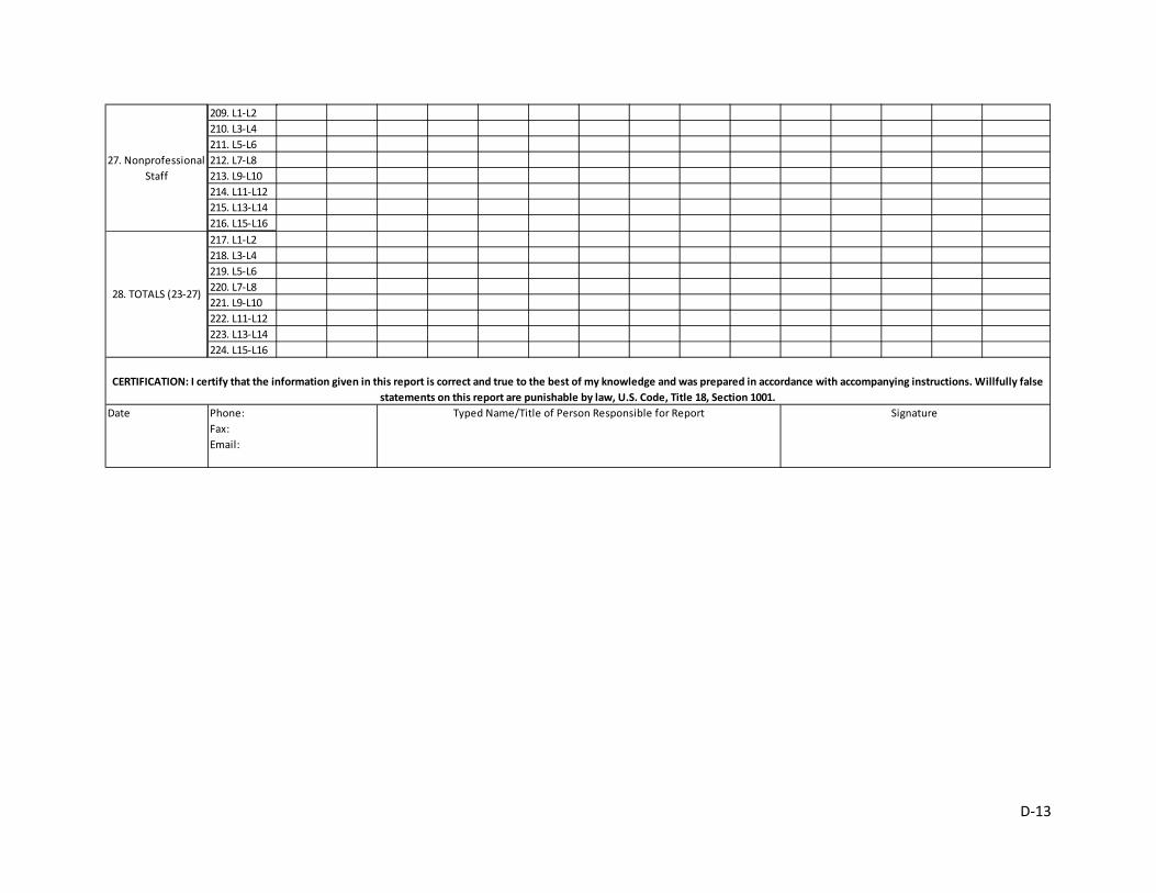
209. L1-L2210. L3-L4211. L5-L6212. L7-L8213. L9-L10214. L11-L12215. L13-L14216. L15-L16217. L1-L2218. L3-L4219. L5-L6220. L7-L8221. L9-L10222. L11-L12223. L13-L14224. L15-L16

Phone:Fax: Email:

27. Nonprofessional Staff

28. TOTALS (23-27)

CERTIFICATION: I certify that the information given in this report is correct and true to the best of my knowledge and was prepared in accordance with accompanying instructions. Willfully false statements on this report are punishable by law, U.S. Code, Title 18, Section 1001.

Date Typed Name/Title of Person Responsible for Report Signature

D-13