final report cie619

1

REPORT OF EXAMPLE 5 BRIDGE PLACED ON A SITE IN TACOMA

Eight-Span Continuous Steel Girder Curved Bridge

Group 6 Course: CIE 619

Structural Dynamics and Earthquake Engineering II

Report Prepared by: Lemuria Pathfinders

Supratik Bose

Sathvika Meenakshisundaram Sharath Chandra Ranganath

Sandhya Ravindran Amy Ruby

2

ACKNOWLEDGEMENTS Lemuria Pathfinders would like to acknowledge that this seismic bridge design

has been adapted from design example 5 in the US Department of

Transportation Federal Highway Administrations Seismic Design of Bridges,

from October 1996. In addition, the original nine span viaduct steel girder bridge

was prepared by BERGER/ABAM Engineers Inc.

-o-o-o-

3

TABLE OF CONTENTS

ACKNOWLEDGMENTS ................................................................................................. 2

LIST OF TABLES ................................................................................................................. 4

LIST OF FIGURES .................................... .......................................................... 5

CHAPTER

1. UNIFORM LOAD METHOD – ELASTIC ANALYSIS ............................................. 12

1.1 General Description of Bridge ............................................................................... 12 1.1.1 Structural System ................................................................................................. 13 1.1.2 Superstructure ...................................................................................................... 14 1.1.3 Substructure ......................................................................................................... 15 1.1.4 Location of Bridge................................................................................................ 17 1.1.5 Site Conditions ..................................................................................................... 18

1.2 Objectives .................................................................................................................. 18

1.3 Modeling Description ............................................................................................. 19 1.3.1 Superstructure ...................................................................................................... 19 1.3.2 Substructure ......................................................................................................... 22

1.4 Initial Elastic Analysis ............................................................................................. 27 1.4.1 Uniform Load Method ........................................................................................ 27 1.4.2 Results and Discussions ...................................................................................... 28

1.5 Summary and Conclusions .................................................................................... 37

2. MODAL ANALYSIS, DEVELOPMENT OF RESPONSE SPECTRA AND SCALING OF GROUND MOTIONS ........................................................................... 39

2.1 Introduction .............................................................................................................. 39

2.2 Eigen Value Analysis .............................................................................................. 39 2.2.1 Natural Periods and Mode Shapes of Structure .............................................. 42 2.2.2 Higher Modes associated with Vibration of Piers .......................................... 44 2.2.3 Comparison with Elastic Analysis Results in SAP 2000 ................................ 45 2.2.4 Analytical Calculations of Bridge Stiffness along local directions ............... 47 2.2.5 Analytical Calculations of Bridge Stiffness along global directions ............. 52

2.3 Response Spectra ..................................................................................................... 54 2.3.1 Seismic Design Spectra ....................................................................................... 55 2.3.2 Seismic Design Spectra of our Site .................................................................... 56

4

2.3.3 Ground Motion Selection ................................................................................... 58 2.3.4 Development of Response Spectra and Scaling of Ground Motions ........... 58

2.4 Development of SDoF Model ................................................................................ 60 2.4.1 Modeling Assumptions....................................................................................... 61 2.4.2 Analysis Procedure .............................................................................................. 62 2.4.3 Results and Discussions ...................................................................................... 62

2.5 Summary and Conclusions .................................................................................... 64

3. UNIFORM LOAD, DYNAMIC MULTIMODE AND PUSHOVER ANALYSIS . 65

3.1 General Overview ................................................................................................... 65

3.2 Uniform Load Method ............................................................................................ 65 3.2.1 Introduction .......................................................................................................... 65 3.2.2 Analysis Procedure .............................................................................................. 66 3.2.3 Results and Discussions ...................................................................................... 68 3.2.4 Summary ............................................................................................................... 72

3.3 Dynamic Multi-Mode Analysis ............................................................................. 72 3.3.1 Introduction .......................................................................................................... 72 3.3.2 Analysis Procedure .............................................................................................. 72 3.3.3 Results and Discussions ...................................................................................... 77

3.4 Push-Over Analysis................................................................................................. 81 3.4.1 Introduction .......................................................................................................... 81 3.4.2 Description of Model ........................................................................................... 82 3.4.3 Plastic Hinge Model ............................................................................................ 84 3.4.4 Non-linear models for pushover analysis ........................................................ 84 3.4.5 Analysis Procedure .............................................................................................. 89 3.4.6 Results and Discussions ...................................................................................... 93 3.4.7 Comparison of stiffness with analytical results ............................................ 101

3.5 Summary and Conclusions .................................................................................. 101

4. TIME HISTORY ANALYSIS ........................................................................................ 103

4.1 General Overview ................................................................................................. 103

4.2 Selected Ground Motions ..................................................................................... 103

4.3 Linear Elastic Time History Analysis ................................................................. 104 4.3.1 Analysis Procedure ............................................................................................ 104 4.3.2 Results 106 4.3.3 Summary ............................................................................................................. 108

4.4 Non Linear Dynamic Time History Analysis .................................................... 109 4.4.1 Introduction ........................................................................................................ 109 4.4.2 Code Specification ............................................................................................. 109

4.5 Non Linear SDoF Time History Analysis .......................................................... 109 4.5.1 Analysis Procedure ............................................................................................ 109 4.5.2 Results 110 4.5.3 Summary ............................................................................................................. 113

4.6 Non Linear MDoF Time History Analysis ......................................................... 113

5

4.6.1 Introduction ........................................................................................................ 113 4.6.2 Description of Model ......................................................................................... 113 4.6.3 Analysis Procedure ............................................................................................ 114 4.6.4 Results and Discussions .................................................................................... 117


5. CAPACITY SPECTRUM AND FLOWCHARTS ...................................................... 124


5.2 Capacity Spectrum Analysis ................................................................................ 124

5.3 Flowcharts .............................................................................................................. 127


6. FINAL CONCLUSIONS................................................................................................ 133


6.2 Comparison from Various Analysis Procedure ................................................ 133

6.3 Performance of Structure ...................................................................................... 135

6.4 Scope of Future work ............................................................................................ 138

6.5 Recommendations for Improvement of Performance ...................................... 138

7. APPENDIX A – VALIDATION OF MODEL ........................................................ 13340

Validation of Elastic Analysis in SAP 2000 ................................................................. 139 Validation of spring stiffness in SAP 2000 .................................................................. 141 Validation of equivalent concrete rectangular section in SAP 2000 ........................ 143 Calibration of Eigen Value Analysis in SAP 2000 ...................................................... 147 Validation of USGS Ground Motion Information and Response Spectra .............. 150 Calibration of SDoF Model in NONLIN Program ..................................................... 151 Calibration of the Program used for Response Spectrum Development ................ 153 Validation of Pushover Analysis and Fiber PMM hinge in SAP 2000 .................... 160

Validation of Time History Analysis .......................................................................... 1647

8. APPENDIX B – TEAM MANAGEMENT PLAN .................................................. 13368

REFERENCES …....................................................................................................................178

-o-o-o-

6

LIST OF TABLES

Table 1.1 Deflection, moment and shear force along the spans under gravity load 30

Table 1.2 Variation of axial forces in superstructure under gravity load .................. 30

Table 1.3 Deflection, moment and shear force along the spans under transverse load ...................................................................................................................... 33

Table 1.4 Maximum resultant forces along piers under transverse load ................... 34

Table 1.5 Maximum resultant forces along piers under longitudinal load on deck 35

Table 2.1 Natural periods and cumulative mass participation of different modes .. 41

Table 2.2 Modal mass participation of first three modes ............................................. 42

Table 2.3 Comparison of periods of the modified bridge and the FHWA original bridge .................................................................................................................. 44

Table 2.4 Calculation of period of bridge from uniform load method ....................... 47

Table 2.5 Deflected shape corresponding to 2nd mode (Transverse) .......................... 48

Table 2.6 Calculation of overall transverse stiffness analytically................................ 48

Table 2.7 Calculation of overall transverse stiffness analytically................................ 51

Table 2.8 Comparison of stiffness of the piers obtained analytically and in SAP 2000.............................................................................................................................. 52

Table 2.9 Calculation of overall stiffness analytically along global direction ........... 53

Table 2.10 Stiffness and mass used in the development of the SDoF model ............... 54

Table 2.11 Response Spectra parameters obtained from USGS .................................... 56

Table 2.12 Scaled ground motions selected from PEER Database ................................ 60

Table 2.13 Results of time history analysis in NONLIN using elastic linear SDoF models along local directions (longitudinal and transverse) ...................... 63

Table 2.14 Results of time history analysis in NONLIN using elastic linear SDoF models along global directions (X and Y) ...................................................... 63

Table 3.1 Summary of uniform load method results obtained from SAP 2000 ........ 69

Table 3.2 Forces, moments and displacements - 100% EE_Trans + 40% EE_long .... 70

Table 3.3 Forces, moments and displacement - 40% EE_Trans + 100% EE_long ..... 70

Table 3.4 Forces, moments and displacements - 100% MCE_Trans + 40% MCE_long.............................................................................................................................. 71

Table 3.5 Forces, moments and displacements - 40% MCE_Trans + 100% MCE_long.............................................................................................................................. 71

Table 3.6 Forces and moments under dead load ........................................................... 77

Table 3.7 Forces and moments for EE - 100% EE_Long + 40% EE_Trans .................. 78

Table 3.8 Forces and moments for EE - 100% EE_Trans + 40% EE_Long .................. 78

7

Table 3.9 Forces and moments for MCE - 100% MCE_Long + 40% MCE_Trans ..... 79

Table 3.10 Forces and moments for MCE - 100% MCE_Trans + 40% MCE_Long ..... 79

Table 3.11 Displacement under Expected Earthquake ................................................... 80

Table 3.12 Displacement under Maximum Credible Earthquake ................................. 80

Table 3.13 Comparison of stiffness .................................................................................. 101

Table 4.1 Selected Ground Motions .............................................................................. 104

Table 4.2 Mass and stiffness values ............................................................................... 104

Table 4.3 Scaled PGA (g) of respective GMs ................................................................ 106

Table 4.4 Resultant forces and displacements in local directions ............................. 106

Table 4.5 Resultant forces and displacements in global directions .......................... 107

Table 4.6 Resultant forces and displacements obtained in linear elastic time history analysis in SAP 2000 program at EE ............................................................. 107

Table 4.7 Resultant forces and displacements obtained in linear elastic time history analysis in SAP 2000 program at MCE......................................................... 108

Table 4.8 Comparison of maximum values recorded for linear time history analysis in SAP 2000 and NONLIN ............................................................................. 108



Table 4.11 Nomenclature used for defining the GMs ................................................... 116

Table 4.12 Maximum resultant forces and displacement recorded at piers during expected earthquake ....................................................................................... 119

Table 4.13 Maximum resultant forces and displacement recorded at piers during maximum credible earthquake ..................................................................... 121

Table 5.1 Comparison of results from various analysis procedure .......................... 126

Table 5.2 Summary of Cc values at EE ........................................................................... 127

Table 5.3 Summary of operational performance level at MCE ................................. 127

Table 5.4 Summary of life safety performance level at MCE ..................................... 127

Table 6.1 Comparison of results from various analysis procedure .......................... 134

Table 6.2 Calculation of R factor at EE and MCE ........................................................ 136

Table 6.3 Performance evaluation of the structure ..................................................... 137

-o-o-o-

8

LIST OF FIGURES

Figure 1.1 Plan View of 8-span continuous; [adapted from FHWA-SA-97-010 Figure 1a] ........................................................................................................................ 12

Figure 1.2 Elevation View of 8-span continuous; [adapted from FHWA-SA-97-010 Figure 1] .............................................................................................................. 13

Figure 1.4 Typical Cross Section; [adapted from FHWA-SA-97-010 Fig 1b] .............. 14

Figure 1.5 Section at Seat-Type-Abutment; [adapted from FHWA-SA-97-010 Fig 1c].............................................................................................................................. 15

Figure 1.6 Intermediate Pier Elevations; [adapted from FHWA-SA-97-010 Fig 1c] ... 16

Figure 1.8 Sliding action of the bearings [adapted from FHWA-SA-97-010 Figure 2].............................................................................................................................. 17

Figure 1.9 Location of the bridge (Source: Google Maps) .............................................. 18

Figure 1.10 Subsurface Soil Conditions; [adapted from FHWA-SA-97-010 Fig A1] .... 18

Figure 1.11 Stick element bridge model in SAP 2000 ....................................................... 19

Figure 1.12 Rigid link element connecting the pier to the superstructure in SAP ....... 21

Figure 1.13 Relationship between actual pier and stick model of 3-D frame elements [adapted from FHWA-SA-97-010] .................................................................. 22

Figure 1.14 Typical view of an intermediate pier in SAP 2000 ....................................... 23

Figure 1.15 Details of sliding bearings at piers [adapted from FHWA-SA-97-010 Figure 10] ............................................................................................................ 24

Figure 1.16 Releases provided in SAP 2000 at top of pier to simulate bearing action . 24

Figure 1.17 Typical plan view of the pile arrangements [adapted from FHWA-SA-97-010] ...................................................................................................................... 25

Figure 1.18 Details of support for spring foundation model [FHWA-SA-97-010 Figure 11] ........................................................................................................................ 26

Figure 1.19 Details of foundation springs in SAP 2000 .................................................... 26

Figure 1.20 Details of abutment supports [FHWA-SA-97-010 Figure 16] ..................... 27

Figure 1.21 Deflected shape of modeled bridge under gravity load .............................. 28

Figure 1.22 Bending moment diagram (major) of modeled bridge under gravity load.............................................................................................................................. 29

Figure 1.23 Shear force diagram (major) of modeled bridge under gravity load ........ 29

Figure 1.24 Settlement of the foundation under pier-1 .................................................... 31

Figure 1.25 Deflected shape of modeled bridge under transverse loading ................... 31

Figure 1.26 Bending moment diagram (major) of modeled bridge under transverse load ...................................................................................................................... 32

Figure 1.27 Shear force diagram (major) of modeled bridge under transverse load ... 32

9

Figure 1.28 Bending moment diagram of modeled bridge under longitudinal load on deck ..................................................................................................................... 35

Figure 1.29 Shear force diagram (major) of modeled bridge under longitudinal load on deck ................................................................................................................ 35

Figure 1.30 Deflected shape of modeled bridge under loangitudinal load ................... 36

Figure 1.31 Bending moment diagram of modeled bridge under longitudinal load on piers ..................................................................................................................... 36

Figure 1.32 Shear force diagram of modeled bridge under longitudinal load on piers.............................................................................................................................. 37

Figure 2.1 Mass source defined for modal analysis in SAP 2000 .................................. 40

Figure 2.2 3D view of the mode shape corresponding to first mode (Longitudinal) 42

Figure 2.3 Plan view of the mode shape corresponding to first mode (Longitudinal).............................................................................................................................. 43

Figure 2.4 3D view of the mode shape corresponding to second mode (Transverse)43

Figure 2.5 Plan view of the mode shape corresponding to second mode (Transverse).............................................................................................................................. 43

Figure 2.6 3D view of the mode shape corresponding to third mode (Torsional) ..... 43

Figure 2.7 Plan view of the mode shape corresponding to third mode (Torsional) .. 44

Figure 2.8 Mode shape corresponding to vibration of pier (4th Mode) ........................ 45

Figure 2.9 Mass Source considering only the weight of the superstructure ............... 46

Figure 2.10 Load applied in local directions for stiffness calculations of 50ft and 70ft piers ..................................................................................................................... 51

Figure 2.11 Displacement recorded in local directions at top of the piers .................... 52

Figure 2.12 Construction of design response spectra using 2-point method [MCEER/ATC 49] ............................................................................................. 54

Figure 2.13 Response Spectra used in the design example .............................................. 55

Figure 2.14 Response Spectra obtained for our site from USGS website for MCE and EE ......................................................................................................................... 57

Figure 2.15 Response Spectra in PEER Ground motion Database .................................. 58

Figure 2.16 Resultant ground motion spectra compared with target spectra in PEER 59

Figure 2.17 Comparison of the mean response spectra of the selected GMs with the target spectra and 85% of target spectra at EE .............................................. 59

Figure 2.18 Comparison of the mean response spectra of the selected GMs with the target spectra and 85% of target spectra at MCE .......................................... 60

Figure 3.1 Distribution of load Po in transverse direction ............................................. 66

Figure 3.2 Distribution of load Po in longitudinal direction .......................................... 66

Figure 3.3 Maximum displacement recorded in transverse direction ......................... 67

Figure 3.4 Maximum displacement recorded in longitudinal direction ...................... 67

Figure 3.5 Response Spectrum function for MCE ........................................................... 74

10

Figure 3.6 Response Spectrum function for EE ............................................................... 74

Figure 3.7 Load case 100 MCE - Long + 40 MCE - Trans ............................................... 75

Figure 3.8 Load case 100 MCE - Trans + 40 MCE - Long ............................................... 75

Figure 3.9 Load case 100 EE - Long + 40 EE - Trans ....................................................... 76

Figure 3.10 Load case 100 EE - Trans + 40 EE - Long ....................................................... 76

Figure 3.11 Column cross-section at base........................................................................... 83

Figure 3.12 Column reinforcement details ......................................................................... 83

Figure 3.13 Pushover Model of the 70 feet pier ................................................................. 84

Figure 3.14 Reinforcement detailing in section designer for the column top section .. 85

Figure 3.15 Reinforcement detailing in section designer for the column bottom section.............................................................................................................................. 85

Figure 3.16 Fiber model of column top in section designer ............................................. 86

Figure 3.17 Fiber model of column base in section designer ........................................... 86

Figure 3.18 Bilinear Stress strain model of concrete ......................................................... 86

Figure 3.19 Non-linear material property of concrete ...................................................... 87

Figure 3.20 Bilinear Stress strain model of rebar ............................................................... 87

Figure 3.21 Material Property input in SAP 2000.............................................................. 87

Figure 3.22 Plastic hinge definition in SAP 2000 program at pier bottom .................... 88

Figure 3.23 Fiber hinge model in SAP 2000 ....................................................................... 88

Figure 3.24 Triangular loading pattern used in SAP 2000 program............................... 89

Figure 3.25 Typical pushover load case in SAP 2000 program ....................................... 90

Figure 3.26 Cross section of the pier considered for Push over analysis ...................... 91

Figure 3.27 Typical plastic hinge assignment at pier bottom in SAP 2000 .................... 92

Figure 3.28 Typical plastic hinge assignment at the column neck in SAP 2000 ........... 93

Figure 3.29 Typical deflected shape of the 70 feet pier in transverse direction ............ 94

Figure 3.30 Force displacement relationship of the 70 feet pier in transverse direction.............................................................................................................................. 94

Figure 3.31 Moment rotation plot of the plastic hinge at the bottom of the 70 feet pier in transverse direction ...................................................................................... 95

Figure 3.32 Typical deflected shape of the 70 feet pier in longitudinal direction ........ 96

Figure 3.33 Force displacement relationship of the 70 feet pier in longitudinal direction .............................................................................................................. 96

Figure 3.34 Moment rotation plot of the plastic hinge at the bottom of the 70 feet pier in longitudinal direction .................................................................................. 97

Figure 3.35 Force displacement relationship of the 50 feet pier in transverse direction.............................................................................................................................. 97

11

Figure 3.36 Moment rotation plot of the plastic hinge at the bottom of the 50 feet pier in transverse direction ...................................................................................... 98

Figure 3.37 Force displacement relationship of the 50 feet pier in longitudinal direction .............................................................................................................. 98

Figure 3.38 Moment rotation plot of the plastic hinge at the bottom of the 50 feet pier in longitudinal direction .................................................................................. 99

Figure 3.39 Typical deflected shape of the pier in transverse direction ........................ 99

Figure 3.40 Force displacement relationship of the bridge in transverse direction ... 100

Figure 3.41 Typical deflected shape of the pier in longitudinal direction ................... 100

Figure 3.42 Force displacement relationship of the bridge in longitudinal direction 101

Figure 4.1 Inputs in NONLIN program for linear analysis along longitudinal direction ............................................................................................................ 105

Figure 4.2 Inputs in NONLIN program for nonlinear analysis along chord direction............................................................................................................................ 110

Figure 4.3 Definition of a time history function in SAP 2000 program ...................... 114

Figure 4.4 Typical Time History Load Case defined in SAP 2000 .............................. 115

Figure 4.5 Type of direct integration procedure followed in SAP 2000 ..................... 115

Figure 4.6 Mass and stiffness coefficients for damping ............................................... 116

Figure 4.7 Definition of mass source for time history analysis ................................... 116

Figure 4.8 Time history load cases defined in SAP 2000 .............................................. 117

Figure 4.9 Maximum displacement response recorded for pier 4 during North Ridge GM ..................................................................................................................... 117

Figure 4.10 Base shear in global X direction with time recorded during North Ridge GM ..................................................................................................................... 118

Figure 4.11 Hysteretic loop of the base shear observed during North Ridge GM ..... 118

Figure 4.12 Hysteretic loop of the plastic moment rotation observed at one of the bottom hinges during North Ridge GM ...................................................... 119

Figure 5.1 Flowchart as applicable to our bridge .......................................................... 131

-o-o-o-

12

CHAPTER 1 1. UNIFORM LOAD METHOD – ELASTIC ANALYSIS

UNIFORM LOAD METHOD – ELASTIC ANALYSIS

1.1 GENERAL DESCRIPTION OF BRIDGE

The bridge being evaluated here is an adapted version of a nine-span viaduct steel

girder bridge, totaling in 1488 feet, presented by a report via the FHWA. The afore-

mentioned bridge has varying span lengths on the left side of the bridge. In addition,

the bridge has expansion joints. The bridge being analyzed in this report is an eight-

span curved continuous bridge, having no expansion joints. The total length of this

bridge is 1384 feet. The eight-spans are a mirror image of the four spans to the right of

the original bridge. All of the properties of the original bridge are mirrored, such that

on each side there are four 173’ spans as shown below in Figure 1.1. The radius of this

curved bridge is 1300 feet. The superstructure consists of four steel plate girders and a

concrete composite cast-in-place deck. The substructure elements, abutments and piers

are all cast-in-place concrete and supported on steel H-piles. The plan and the elevation

views are shown in Figure 1.1 and Figure 1.2.

Figure 1.1 Plan View of 8-span continuous; [adapted from FHWA-SA-97-010 Figure 1a]

13

Figure 1.2 Elevation View of 8-span continuous; [adapted from FHWA-SA-97-010 Figure 1]

1.1.1 Structural System

The structural system of the bridge can be classified into two broader sections:

superstructure and the substructure. The superstructure consists of the deck and the

steel girders while the substructure comprises the abutments and pier columns, pile

foundations and bearings to connect the piers to the girders. The load from the deck is

transferred to the girders which transfer the entire load to the foundation through

bearings thus acting as a rigid element.

14

1.1.2 Superstructure

The two main components of the superstructure to be designed and analyzed are the

deck and the girder. The deck is simply the surface of the bridge on which the vehicles

run. It’s generally made of concrete covered with another layer of asphalt concrete or

pavement to account for the wearing of the surface due to friction and damage from the

vehicle loads. In the present project, also the bridge is made of concrete. The deck is

supported on steel girders which effectively take the loads of the vehicles running on

the deck and the self-weight of the deck itself. In this case the bridge has ‘I’ shaped steel

sections for girders.

The geometric properties of the superstructure are as follows:

The bridge consists of eight spans, with all the spans 173 feet long. The right four

spans are mirror image of the other four spans.

The width and thickness of the deck is 42 ft and 9 inch throughout the length of

the bridge.

The bridge slab is made of concrete of characteristic compressive strength 4 ksi

and supported by four steel girders.

Chevron bracings are provided to connect the girders to the deck. The bracings

are used to transfer the lateral internal load of the superstructure to the bearing.

The cross-section of the superstructure is shown below in Figure 1.3.

Figure 1.3 Typical Cross Section; [adapted from FHWA-SA-97-010 Fig 1b]

15

1.1.3 Substructure

The substructure of a bridge is mainly used to transfer the loads from the superstructure

to the soil through the foundation and is a combination of all the components that

support the superstructure. It mainly consists of abutments, piers, piles and bearings.

Abutments

Abutments are the part of the substructure which, in case of a multi-span bridge,

supports the ends near the approach slab. They are meant to resist and transfer loads

like the self-weight, lateral loads (wind loads) and the ones from the superstructure to

the foundation elements. The abutments are mainly provided in the design bridge to

accommodate the thermal movement of the superstructure which will also allow for a

tolerance of movement in the longitudinal direction, and restraint in the transverse

direction. A clearance of 4 in was provided at the end of the girder-abutment connection.

The typical cross-section of a seat-type abutment of the design bridge is presented in

Figure 1.4.

Figure 1.4 Section at Seat-Type-Abutment; [adapted from FHWA-SA-97-010 Fig 1c]

16

Piers

When bridges are too long to be supported by abutments alone, that is, in case of multi-

span bridges the intermediate support is provided by piers which are built like walls

shaped like girders. Piers are supported by elements called piles. These are slender

columns that are generally placed in a group to support loads transferred from the piers

via a pier cap. They are designed in such a way that they support loads through bearing

at the tip, friction along the sides, adhesion to the soil or a combination of all these.

Figure 1.5 shows the elevation of the piers of the design bridge.

Figure 1.5 Intermediate Pier Elevations; [adapted from FHWA-SA-97-010 Fig 1c]

Bearings

The devices that transfer the loads and movements from the deck to the substructure

and the foundation are called bearings. These movements are accommodated by the

basic mechanisms of internal deformation (elastomeric), sliding (PTFE) or rolling.

17

Conventional types of pinned bearings are assumed at the piers 2, 3, 5 and 6 to ensure

transfer of both longitudinal and transverse seismic forces to the substructure through

anchor bolts. For the piers 1, 4 and 7 bearings were provided to accommodate expected

displacements. Elastomeric bearing with provisions for sliding between the bearing and

girder under large displacements was used for this purpose. Polytetraflouralethylene

(PTFE) bearings were provided against the sliding surface (stainless steel). In addition,

no expansion joints are present in the modified bridge used in the present project.

Figure 1.6 Sliding action of the bearings [adapted from FHWA-SA-97-010 Figure 2]

Figure 1.6 shows the action of the bearings during longitudinal deflection. During

longitudinal loads only the pinned piers (Pier 2,3,5,6) participate and the piers with

elastomeric bearing will slide (Pier 1,4,7) without resisting any longitudinal forces.

However transverse shear will be transferred in all the bearings during transverse

loading.

It is also to be noted that the values and numbering systems in the figures taken from

the previous report done by the FHWA do not necessarily coincide with the numbering

system and calculated values for this configuration. The height of the middle five and

outer two piers will be 70’ and 50’, respectively and enclosed between two abutments,

one on either side.

1.1.4 Location of Bridge

The bridge is located at coordinates 47.2663 N and 122.395105 W, in Tacoma,

Washington. Figure 1.7 present the location of the bridge from google maps. Tacoma is

a mid-sized port city named after the nearby Mount Rainier, originally called Mount

Tahoma. Known as the ‘City of Destiny’ because it was chosen to be the western

terminal of the Northern Pacific Railroad in the late 19th century.

18

The Tacoma fault, is an active east-west striking north dipping reverse fault with close

to 35 miles of identified surface rupture, capable of generating earthquakes of atleast

magnitude 7.

Figure 1.7 Location of the bridge (Source: Google Maps)

1.1.5 Site Conditions

Although the soil in Tacoma, Washington is generally gravelly loam, for purpose of

analysis, the soil conditions will be taken as the same as the conditions given in the

FHWA report. Therefore, the soil profile will be taken as Type I- “Stable deposits of

sands and gravels where the soil depth is less than 200 feet.” The soil properties are

summarized in the Figure 1.8.

Figure 1.8 Subsurface Soil Conditions; [adapted from FHWA-SA-97-010 Fig A1]

1.2 OBJECTIVES

The bridge analyzed here is the fifth of seismic design examples developed using

AASHTO for the FHWA. The bridge was relocated in Tacoma nearby Mount Rainer

from Pacific Northwest to evaluate the seismic performance of the bridge. The analysis

19

presented in the present project was done in accordance with the provisions of MCEER-

ATC/49 document and AASHTO 2009 LRFD Seismic Design Guide Specifications.

The primary objective was to evaluate the bridge response using various analysis

procedures given in the codes and compare the results obtained from them and critical

assessments were made from the results. The elastic analysis approach based on

uniform load method is carried out in the present chapter and the results are presented.

1.3 MODELING DESCRIPTION

The bridge model was developed in a commonly used structural analysis program SAP

2000 v. 16.0.1 [CSI, 2009].

Figure 1.9 shows the stick model used to simulate its behaviour in SAP 2000 program in

which single line frame elements were used for both superstructure and intermediate

piers. The nodes and the work line elements were located at the center of gravity of the

superstructure, which is 8 feet above the top of the piers. Dimensions of the bridges are

presented earlier in the report.

Figure 1.9 Stick element bridge model in SAP 2000

1.3.1 Superstructure

Some the basic modeling assumptions are listed as follows:

Only bridges which subtend an angle of more than 30 degrees are required to be

analyzed as a curved structure, else they are allowed be analyzed as a straight

20

one. In our case, the bridge has a span of 1384 ft (173*8) and a radius of curvature

of 1300 ft, thus subtending an angle of theta= 1384/1300 = 1.065 radians = 60.097

degrees> 30 degrees. Therefore, the superstructure of the bridge was analyzed

using the actual curved geometry.

The bridge superstructure considered in this project has 8 spans over which a

uniformly distributed load (dead load) of 9.3 kips/feet was acting. The

calculations for the dead load are similar to the design example 5 and presented

as follows.

Weight of the superstructure is calculated as following:

concrete 0.15 kip/feet3 Unit weight of concrete

Deck 42’ X 9 “ Width and thickness of bridge deck

wslab 5 kip/feet Weight of concrete deck and girder pads

wsteel 1.9 kip/feet Weight of steel plate girders and cross

frames

wmisc 2.4 kip/feet Weight of barriers, stay-in-place metal

forms and future overlay

wsuper = wslab + wsteel + wmisc

wsuper 9.3 kip/feet Weight per length of the superstructure

The superstructure is a composite structure comprising of I shaped steel girders

and a concrete deck. To simulate this model in SAP 2000, we consider an

equivalent concrete cross-section which has the same Area and Moment of

Inertia as that of the composite cross section. The modifiers used to model the

superstructure is calculated in the succeeding sections

While analyzing ,the additional loads due to traffic barriers, wearing surface

overlay and stay-in-place metal forms are included and taken to be 2.4 kips per

lineal foot of superstructure.

To account for the height of the bearings and the levelling pedestal, the centroid

of the superstructure is taken at a height of 8 feet above the top of the pier. The

girders are modeled as rigid link element in SAP 2000 program which was done

21

by providing end length offset to the elements with rigid zone factor 1 indicating

full rigidity (Figure 1.10).

To compute the bending stiffness full composite action between deck and girder

was assumed. The slipping at higher levels of loadings were neglected.

The torsional properties are simulated considering that only the deck was

effective in providing torsional stiffness.

Strength of concrete was taken to be 4000 psi, while steel was assumed to be

A615Gr60. Uncracked section properties were used to determine area and

moments of inertia assuming full composite action between deck and girders.

Figure 1.10 Rigid link element connecting the pier to the superstructure in SAP

Mass and Stiffness property of superstructure

In the design example, the spans are divided into four parts and the masses are lumped

in the nodes based on tributary area consideration. However, in SAP 2000 program, the

superstructure is modelled as frame elements with each span divided into eight stations.

Also, the gravity load calculated as 9.3 kips/feet (same as the design example 5 as the

cross-section of the superstructure remains same) was applied as uniformly distributed

throughout the spans. So, masses were not needed to be lumped at the nodes in SAP

2000 model.

Calculation of modifiers used in SAP 2000 to model the superstructure

For analysis, the deck and girder are considered to be a composite concrete structure

which has the same Area and the moment of inertia as that of the composite beam. Also

the torsional constant of the deck alone was used to model the superstructure.

Rigid Link

22

For this we consider the composite section to be a square and thus calculate its width as

follows:

Area of the composite section = b2 = 60 ft2

Calculation was done by equating MIX of the transformed section to that of the actual

section

Moment of Inertia about horizontal axis= 518 ft4

= b^4/12

= b = 8.879 ft ~ 8.8 ft

Therefore, the Area modifier = 60 / 8.8792 = 0.76

The moment about the Y axis is given to be 9003 ft4.

The modifier used for Moment of Inertia along vertical axis = 9003/518 = 17.37.

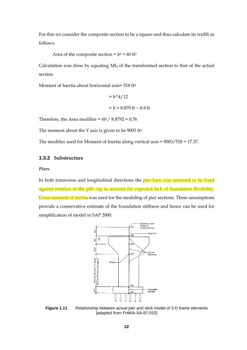
1.3.2 Substructure

Piers

In both transverse and longitudinal directions the pier base was assumed to be fixed

against rotation at the pile cap to account for expected lack of foundation flexibility.

Gross moment of inertia was used for the modeling of pier sections. These assumptions

provide a conservative estimate of the foundation stiffness and hence can be used for

simplification of model in SAP 2000.

Figure 1.11 Relationship between actual pier and stick model of 3-D frame elements [adapted from FHWA-SA-97-010]

sharathchandra

Highlight

sharathchandra

Highlight

23

The intermediate piers are modeled as 3D frame elements that represent the represent

the individual columns. The relationship between the stick element and the actual pier

cross section is presented in Figure 1.11. Three elements were used to model the pier in

SAP 2000 to take into account the varying cross-section by interpolating between the

member end notes. All the properties are based on uncracked sectional details.

Foundation stiffness were attached to the bottommost nodes of the piers (2XX) by means

of spring supports. The intermediate pier modeled in SAP 2000 program is shown in

Figure 1.12.

Figure 1.12 Typical view of an intermediate pier in SAP 2000

Connection of piers to superstructure

In the actual bridge, the internal forces are transferred from the superstructure to the

piers through the bearings. In the SAP 2000 program, the forces are transferred through

a single point where the superstructure and the pier intersects, node 6XX in Figure 1.11.

At the pinned piers, node 6XX transfers shears in all directions from the superstructure,

but is released in moment along longitudinal direction. To account for this, the M3

moment is released at the top of the piers in SAP 2000 program (Figure 1.14). The other

sliding piers with elastomeric bearing are free to move longitudinally and hence only

transverse shear were transferred. So, in addition to M3, V2 are also released at the top

of those piers.

sharathchandra

Highlight

24

Figure 1.13 Details of sliding bearings at piers [adapted from FHWA-SA-97-010 Figure 10]

Translational and rotational releases were provided at the top of the piers with sliding

bearings to allow unrestrained longitudinal motion. The releases were made in local

coordinate system in SAP 2000 program to ensure its tangential orientation with respect

to the point of curvature at the center of the pier.

Figure 1.14 Releases provided in SAP 2000 at top of pier to simulate bearing action

Foundation Stiffness’s

Generally, soil contribution under a pile cap is not included because it is assumed that

soil will settle away from the cap. The piers are assumed to be located in flood plain of

a large river. The scour and loss of contact of soil around and beneath the pile cap, only

sharathchandra

Highlight

25

the stiffness of the pile group will be considered and the resulting forces at the

foundation level will only be applied to pile group to determine design loads to the pile.

Flexibility of pile cap is also neglected. To compute linear springs, elastic subgrade

approach is used as described in the seismic design, FHWA.

Since the relative stiffness of the foundation to the stiffness of the pier column is very

large, the resulting force for design of the pier and foundations will not vary

significantly, generally less than 5 percent. Generally, any reasonable development of

spring stiffness will produce acceptable results.

Considering he pile group, as shown in Figure 1.15, the foundation stiffness is calculated

in FHWA-SA-97-010. As the soil conditions are similar to the design example 5, the

spring stiffness obtained for foundation can be directly used in SAP 2000 model. Figure

1.16 and Figure 1.17 shows the modeling of foundation stiffness. The values of the

spring constants used in SAP 2000 program are as follows:

k11 2.66 × 104 Kip/ft

k22 7.847 × 105 Kip/ft

k33 1.70× 104 Kip/ft

k44 7.96 × 107 Kip-ft/rad

k55 4.785 × 106 Kip-ft/rad

K66 9.628 × 107 Kip-ft/rad

Figure 1.15 Typical plan view of the pile arrangements [adapted from FHWA-SA-97-010]

sharathchandra

Highlight

26

Figure 1.16 Details of support for spring foundation model [FHWA-SA-97-010 Figure 11]

Figure 1.17 Details of foundation springs in SAP 2000

Abutments

The abutments were modeled as simple nodes with a combination of full restraints

(vertical translation and superstructure torsional rotation) and an equivalent spring

stiffness along transverse direction as shown in Figure 1.18. The calculation of the spring

stiffness was based on the pile stiffness of the intermediate piles and it was similar to

the one calculated in design example 5. Spring stiffness of 4663.64 kips/feet was

provided in transverse direction to model the abutments in SAP 2000 program. The

restraints and the springs are all provided relative to the local coordinate geometry.

sharathchandra

Highlight

27

Figure 1.18 Details of abutment supports [FHWA-SA-97-010 Figure 16]

1.4 INITIAL ELASTIC ANALYSIS

1.4.1 Uniform Load Method

The objective of the uniform load method is to estimate the displacement demand for

the simplistic model of the superstructure done in SAP 2000 program. In this analysis

procedure, the structure was subjected to gravity load (9.3 kips/feet) only considering

the weight of the superstructure and an arbitrary distributed load (40 kip/feet) applied

both longitudinally and transversely, separately, to study the behaviour of bridge

subjected to longitudinal and transverse forces.

The following basic assumptions were made during elastic analysis in SAP 2000

The superstructure was subjected to uniformly distributed load of 40 kips/feet

to ensure high workable displacement.

Linear elastic analysis was done, no plastic hinges were assumed to be formed

throughout the analysis.

Lateral load along transverse direction was subjected only on the superstructure

while the lateral load along longitudinal direction was subjected both on the

superstructure and piers separately.

sharathchandra

Highlight

28

1.4.2 Results and Discussions

The bridge modeled in SAP 2000 program was subjected to both gravity load and lateral

loads and elastic analysis was performed. The results obtained from the analysis in

terms of deflected shapes, bending moment and shear forces are discussed in this

section. As seen from the Figure 1.19 to Figure 1.30, the bridge behave symmetrically

under the gravity load which further validate the model produced in SAP 2000 to

simulate the bridge behaviour.

Gravity Load

The deflected shape, bending moment and shear force diagrams under gravity load of

9.3 kips/feet are presented in Figure 1.19 to Figure 1.21. The deflection observed was

more along the end spans compared to the intermediate spans as expected. Maximum

displacement of 0.25 feet was observed under the gravity loads at the end spans. The

bending moment and shear force diagrams obtained for the bridge model are similar to

that obtained for a multi-span continuous beam, which was expected. Also, it was

observed that there was no deflection at the nodes of the superstructure, as rigid

elements were considered to model the girders thereby allowing zero displacement.

Table 1.1 shows the deflection, bending moment and shear force in the spans under

gravity load. As the bridge is symmetric in geometry only the first four spans were

considered for critical assessment of the bridge. The maximum values were also

obtained and presented in the Tables so that the critical sections can be identified.

Figure 1.19 Deflected shape of modeled bridge under gravity load

sharathchandra

Highlight

29

Figure 1.20 Bending moment diagram (major) of modeled bridge under gravity load

Figure 1.21 Shear force diagram (major) of modeled bridge under gravity load

30

Table 1.1 Deflection, moment and shear force along the spans under gravity load

Span Location Deflection

(feet)

Bending Moment

(Kips-feet)

Shear Force (Kips)

Gra

vit

y L

oad

ing

Span-1

Left 0 -2504.1 -694.4

Middle 0.25 22225.2 161.2

Right 0 -32125.2 1020.25

Maximum 0.25 32125.2 1020.25

Span-2

Left 0 -30325.3 -863.2

Middle 0.06 9555.0 -54.1

Right 0 -21050.7 756.0

Maximum 0.06 -30325.3 -863.2

Span-3

Left 0 -21213.5 -778.3

Middle 0.08 11290.3 12.3

Right 0 -21817.0 785.5

Maximum 0.08 -21817.0 785.5

Span-4

Left 0 -21799.2 -774.3

Middle 0.07 10381.2 -11.7

Right 0 -20944.8 763.9

Maximum 0.07 -21799.2 -774.3

It can be seen from the Table 1.1, that maximum deflection for all the spans were

observed at the middle with the value maximum for end span. Negative moments were

observed at all the supports, while positive bending moment were observed at the

middle, indicating double curvature bending of the spans. Also, it was observed that

for all the spans the bending moments and shear forces are maximum at the same

sections, mostly along the girder supports. Maximum shear force and moment was

observed at the right end of the first span.

Table 1.2 Variation of axial forces in superstructure under gravity load

Spans Span-1 Span-2 Span-3 Span-4

Axial Force (Kips) 12.7 24.9 17.1 17.9

Resultant Torsion (kips-feet) -4321.1 700.2 -342.2 261.1

31

Figure 1.22 Settlement of the foundation under pier-1

The variation of the axial forces under gravity load was not much, however it can be

seen from Table 1.2, that the superstructure was subjected to some amount of torsion

under gravity loading. Figure 1.22 shows the settlement of the foundation at the pier-1.

There was slight settlement observed in the foundations of the order of 0.0010 feet, as

they were not modelled as fixed supports. The restraints were provided in form of

spring constants as described earlier. Similar observations were also made with the

other foundation supports.

Transverse Load

A transverse load of 40 kips/feet was applied along the superstructure throughout the

entire length of the bridge. The deflected shape, bending moment and shear force

diagrams under transverse load are presented in Figure 1.23 to Figure 1.25. As it can be

seen from the deflected shape, the entire superstructure moves like a rigid body in the

direction of the force. Maximum deflection of 1.36 feet was observed at the center of the

bridge as expected.

Figure 1.23 Deflected shape of modeled bridge under transverse loading

sharathchandra

Highlight

32

Figure 1.24 Bending moment diagram (major) of modeled bridge under transverse load

Figure 1.25 Shear force diagram (major) of modeled bridge under transverse load

33

Table 1.3 Deflection, moment and shear force along the spans under transverse load

Span Location Absolute

Deflection (inch)

Bending Moment

(Kips-feet)

Shear Force (Kips)

Tra

nsv

erse

Lo

adin

g

Span-1

Left 0 0 -2055.9

Middle 0.87 71364.8 565.0

Right 0.81 -106905.9 3401.6

Maximum 0.87 -106905.9 3401.6

Span-2

Left 0.86 -106904.5 -2668.5

Middle 0.89 3298.9 133.1

Right 0.92 -137042.6 3140.7

Maximum 0.92 -137042.6 -2668.5

Span-3

Left 0.96 -137047.9 -3518.9

Middle 1.11 34346.2 -543.1

Right 1.22 -45548.6 2504.9

Maximum 1.22 -135047.9 -3518.9

Span-4

Left 1.24 -45555.2 -3076.3

Middle 1.35 81644.6 0

Right 1.36 -43980.1 3081.3

Maximum 1.36 81644.6 3081.3

As it can be observed from Table 1.3, the deflection of the superstructure was observed

to be more or less similar throughout the length of the beam with the maximum value

being observed at the end of span 4, which is actually the center point of the bridge. The

maximum bending moment and shear force was observed at same sections with one

exception in span 4. Again change in sign of bending moment and shear force was

observed indicating double curvature bending. In almost all the cases the maximum

resultant forces were recorded at the supports as also observed under gravity load. So

the sections near the girder support are critical sections and needs tension reinforcement

at the top as negative bending moment (hogging) was observed both during transverse

and gravity loading.

sharathchandra

Highlight

34

Table 1.4 Maximum resultant forces along piers under transverse load

Piers Shear(kips) Moment (kips-feet)

Displacement (feet) Axial force

(kips) Long Trans Trans Long Long Trans

Left Abut 285.3 3115.9 0.0 1095.3 0.60 0.65 51.8

Pier 1 0.0 7098.1 405837.3 0.0 0.49 0.97 797.6

Pier 2 1393.0 7502.9 490020.7 80793.5 0.35 1.11 1165.0

Pier 3 361.3 6218.5 509082.6 28182.6 0.19 1.39 782.3

Pier 4 0.0 6696.7 547189.6 0.0 0.00 1.50 253.6

Pier 5 35.0 6309.6 514862.2 2724.7 0.19 1.39 754.4

Pier 6 952.3 7518.7 491541.5 55232.9 0.35 1.11 1142.9

Pier 7 0.0 7105.7 406414.8 0.0 0.49 0.97 797.6

Right Abut 285.0 3115.4 0.0 1097.1 0.61 0.65 51.8

Table 1.4 presents the maximum resultant forces in the piers under transverse load both

in its weak and strong direction. The resultant forces were observed to be more in its

strong direction compared to weak direction, as the load was applied along transverse

direction. High negative moment was observed along the piers in strong direction with

the pier-4 having maximum value. The bending moment in the piers are much higher

than the superstructure as evident from Figure 1.24 and Table 1.4. The deflection of the

pier along the direction of loading increases from the ends to the center with a maximum

displacement of 1.00 feet at the center pier. However, along weak direction the

deflection of the pier is not varying much.

Longitudinal Load on Superstructure

Longitudinal load of 40 kips/feet was applied to the superstructure of the bridge to

investigate its behaviour under longitudinal forces. Thus it can be seen from the Figure

1.26 and Figure 1.27 that the siding piers (pier 1, 4 and 7) don’t participate in the

longitudinal direction which is in accordance with the assumption made in Figure 2 of

FHWA design example. In order to take into account the sliding action of those piers

only transverse shear was transferred and hence no shear and bending moment was

observed under longitudinal loading in the corresponding piers.

sharathchandra

Highlight

35

Figure 1.26 Bending moment diagram of modeled bridge under longitudinal load on deck

Figure 1.27 Shear force diagram (major) of modeled bridge under longitudinal load on deck

Table 1.5 Maximum resultant forces along piers under longitudinal load on deck


Displacement (feet) Axial force


Left Abut 46.8 165.7 0.0 102.6 5.75 0.04 2.8

Pier 1 0.0 786.5 40110.1 0.0 5.72 0.12 280.0

Pier 2 19407.5 403.5 24143.2 1125633.3 5.65 0.07 84.3

Pier 3 8243.4 192.2 3540.7 642988.9 5.66 0.03 470.8

Pier 4 0.0 877.4 38889.6 0.0 5.68 0.00 1341.6

Pier 5 8192.2 2545.3 159735.9 638990.5 5.66 0.03 1917.7

Pier 6 19181.3 501.2 3814.0 1112512.6 5.65 0.07 1291.7

Pier 7 0.0 907.3 42467.7 0.0 5.72 0.12 573.3

Right Abut 82.3 231.2 0.0 102.6 5.75 0.04 3.8

36

Longitudinal Load on Piers

Longitudinal load of 40 kips/feet was applied to the piers to investigate the behaviour

bridge under longitudinal forces. The load was applied in SAP 2000 program in global

X direction along the piers, therefore, it was not applied in purely longitudinal direction

due to curved geometry. Hence, some transverse displacement was also evident from

the Figure 1.28. As it can be seen from the Figure 1.29 and Figure 1.30, the bending

moments and shear forces were maximum at the pier bottom, where the foundation

stiffness’s were provided. Also, the resultant forces (V and M) was more in the piers

compared to the superstructure. This was mainly because, the deflection of the

superstructure was much less compared to that of the piers.

Figure 1.28 Deflected shape of modeled bridge under loangitudinal load

Figure 1.29 Bending moment diagram of modeled bridge under longitudinal load on piers

sharathchandra

Highlight

37

Figure 1.30 Shear force diagram of modeled bridge under longitudinal load on piers

1.5 SUMMARY AND CONCLUSIONS

A uniform load method of analysis was used to get response of a simplified model of

the bridge in SAP 2000 program. The general description of the bridge and assumptions

made in the model are discussed in details and the results obtained from the analysis

are presented. The bridge used in the project is symmetric in geometry and hence

symmetry is also observed in the resultant forces. It can be observed that all the bending

moment and shear force diagrams are symmetric in nature. The behaviour of the bridge

under gravity and lateral loads can be summarized as follows:

The superstructure of the bridge almost behave as a rigid body under transverse

loading with partial restrain at both abutment and at pier location.

Maximum deflection was observed at the end spans under gravity loading, however

the deflection was maximum at the center of the bridge under transverse loading.

The bending moment diagrams indicated that the superstructure was under double

curvature bending both under gravity and transverse loads.

Maximum shear forces and bending moments were observed at the girder supports

for both gravity and transverse loading.

The maximum displacement of the superstructure observed in transverse direction

for 40 kips/feet of uniformly distributed load was 1.36 feet, while the maximum

deflection was observed to be 0.25 feet for gravity loading.

sharathchandra

Highlight

sharathchandra

Highlight

sharathchandra

Highlight

sharathchandra

Highlight

38

The maximum deflection of the substructure (pier 4) was 1.00 feet under transverse

direction along the direction of loading.

The variation in axial force in the superstructure was not much due to gravity load

along the length of the bridge. However, torsional moments were present in the

superstructure under the action of gravity loads.

It was also observed that the foundation nodes have undergone some settlement, as

springs were used for modeling.

-o-o-o-

39

CHAPTER 2 2. MODAL ANALYSIS, DEVELOPMENT OF RESPONSE SPECTRA AND SCALING OF GROUND MOTIONS

MODAL ANALYSIS, DEVELOPMENT OF RESPONSE SPECTRA AND SCALING OF

GROUND MOTIONS

2.1 INTRODUCTION

In the previous chapter, the general description of the bridge was presented and its

behaviour under generic lateral load, both transverse and longitudinal, was

investigated. Therefore, the two principle directions were considered for analysis. In

this chapter multimode analysis of the bridge is carried out in SAP 2000 program

considering all the modes which contribute significantly to the overall behaviour of the

structure. The response spectra for our site (Tacoma) has been obtained for both design

earthquake (DE) and maximum credible earthquake (MCE). A suite of ground motions

is selected for time history analysis and scaled by comparing their corresponding

response spectra to the design spectra for our site. Further, a simplified single degree of

freedom (SDoF) model of the bridge was developed in NONLIN software to examine

its behaviour and compared with the response obtained in SAP 2000 program.

2.2 EIGEN VALUE ANALYSIS

The model developed in SAP 2000 program for the analysis using uniform load method

(described in previous chapter) is also used for the multimode method of analysis and

therefore, the same modeling assumptions are valid. The load considered for the modal

analysis in SAP 2000 program is the total dead load of the superstructure coming from

the element self-weight. The live load and other miscellaneous loads are neglected in

40

modal analysis to avoid complications. The load of the structure is defined in SAP 2000

by defining mass source as shown in Error! Reference source not found..

Figure 2.1 Mass source defined for modal analysis in SAP 2000

The maximum number of modes were initially set to 12 in SAP 2000 program, as it was

expected that the modal participation factor of the first 12 modes will be greater than

90%. However, as the analysis was carried out, it was observed that about 83 Eigen

values were needed to capture 100% mass participation in both translation and rotation

along all the three directions. However, modal participation factor of 90% was observed

in the 27th mode for the principle directions (X and Y). Therefore, the results obtained

from the first 30 modes are shown in Table 2.1 to also demonstrate the contribution of

the higher modes on the structure. The natural periods and the corresponding mode

shapes are presented in the succeeding sections. It can be seen from Table 2.1, that the

cumulative modal mass participation had reached 90% first in rotation along vertical

axis at 13th mode, while for translational motion it is reached only after 20th and 27th

modes for transverse and longitudinal directions, respectively.

41

Table 2.1 Natural periods and cumulative mass participation of different modes

Mode Period

(s)

Cumulative Modal Mass Participation

SumUX SumUY SumUZ SumRX SumRY SumRZ

1.00 1.54 0.57 0.00 0.00 0.00 0.00 0.06

2.00 0.88 0.57 0.59 0.00 0.02 0.00 0.06

3.00 0.75 0.62 0.59 0.00 0.02 0.00 0.60

4.00 0.75 0.67 0.59 0.00 0.02 0.00 0.60

5.00 0.71 0.67 0.59 0.00 0.02 0.02 0.60

6.00 0.69 0.67 0.87 0.00 0.03 0.02 0.60

7.00 0.68 0.67 0.87 0.01 0.09 0.02 0.60

8.00 0.62 0.70 0.87 0.01 0.09 0.02 0.89

9.00 0.62 0.70 0.87 0.01 0.09 0.07 0.89

10.00 0.54 0.70 0.87 0.03 0.18 0.07 0.89

11.00 0.52 0.70 0.88 0.03 0.18 0.07 0.89

12.00 0.48 0.70 0.88 0.03 0.18 0.15 0.89

13.00 0.45 0.76 0.88 0.03 0.18 0.15 0.90

14.00 0.45 0.78 0.89 0.03 0.18 0.15 0.91

15.00 0.43 0.78 0.89 0.03 0.18 0.15 0.93

16.00 0.43 0.78 0.89 0.07 0.35 0.15 0.93

17.00 0.39 0.78 0.89 0.07 0.35 0.47 0.93

18.00 0.37 0.78 0.89 0.42 0.38 0.47 0.93

19.00 0.36 0.78 0.89 0.42 0.38 0.47 0.93

20.00 0.31 0.78 0.91 0.42 0.42 0.47 0.93

21.00 0.30 0.78 0.91 0.42 0.42 0.47 0.93

22.00 0.30 0.78 0.91 0.42 0.43 0.47 0.93

23.00 0.27 0.78 0.95 0.42 0.52 0.47 0.93

24.00 0.27 0.86 0.95 0.42 0.52 0.47 0.93

25.00 0.27 0.86 0.96 0.42 0.56 0.47 0.93

26.00 0.27 0.86 0.96 0.42 0.56 0.47 0.94

27.00 0.26 0.90 0.96 0.42 0.56 0.47 0.94

28.00 0.25 0.96 0.96 0.42 0.56 0.47 0.95

29.00 0.24 0.96 0.97 0.42 0.56 0.47 0.95

30.00 0.24 0.96 0.97 0.42 0.57 0.47 0.95

42

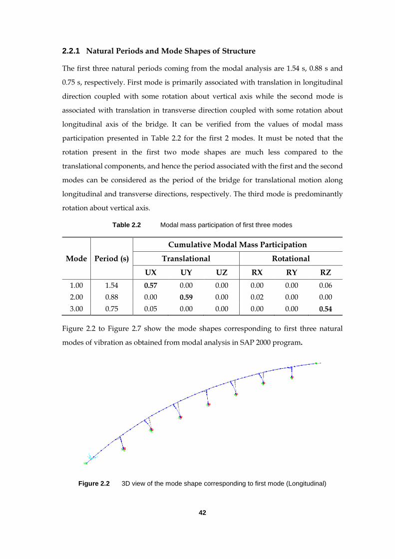
2.2.1 Natural Periods and Mode Shapes of Structure

The first three natural periods coming from the modal analysis are 1.54 s, 0.88 s and

0.75 s, respectively. First mode is primarily associated with translation in longitudinal

direction coupled with some rotation about vertical axis while the second mode is

associated with translation in transverse direction coupled with some rotation about

longitudinal axis of the bridge. It can be verified from the values of modal mass

participation presented in Table 2.2 for the first 2 modes. It must be noted that the

rotation present in the first two mode shapes are much less compared to the

translational components, and hence the period associated with the first and the second

modes can be considered as the period of the bridge for translational motion along

longitudinal and transverse directions, respectively. The third mode is predominantly

rotation about vertical axis.

Table 2.2 Modal mass participation of first three modes

Mode Period (s)

Cumulative Modal Mass Participation

Translational Rotational

UX UY UZ RX RY RZ

1.00 1.54 0.57 0.00 0.00 0.00 0.00 0.06

2.00 0.88 0.00 0.59 0.00 0.02 0.00 0.00

3.00 0.75 0.05 0.00 0.00 0.00 0.00 0.54

Figure 2.2 to Figure 2.7 show the mode shapes corresponding to first three natural

modes of vibration as obtained from modal analysis in SAP 2000 program.

Figure 2.2 3D view of the mode shape corresponding to first mode (Longitudinal)

43

Figure 2.3 Plan view of the mode shape corresponding to first mode (Longitudinal)

Figure 2.4 3D view of the mode shape corresponding to second mode (Transverse)

Figure 2.5 Plan view of the mode shape corresponding to second mode (Transverse)

Figure 2.6 3D view of the mode shape corresponding to third mode (Torsional)

44

Figure 2.7 Plan view of the mode shape corresponding to third mode (Torsional)

For comparison of the multi-mode analysis results obtained in SAP 2000 program with

the periods obtained in FHWA Design Example 5, the results are presented in Table 2.3.

It can be seen from the Table that the results obtained from SAP 2000 program are in

close agreement with the results obtained in the design example. The longitudinal

periods of unit-1 and unit-2 of the original bridge in the design example are 1.52 s and

1.20 s respectively. Since the modified bridge analyzed in this project is eight span

bridge similar to the unit-2 of the original bridge, therefore its longitudinal period

obtained from modal analysis in SAP 2000 matches closely with that obtained for Unit-2

of the design example. In addition, the period associated with translational motion in

transverse direction is also similar in both SAP 2000 and the design example. However,

the small difference is due to presence of expansion joints in the original bridge.

Therefore, the similarity in time periods of the bridge in principle directions obtained

from SAP 2000 with the periods of the original bridge presented in FHWA design

example further validates our model.

Table 2.3 Comparison of periods of the modified bridge and the FHWA original bridge

SAP 2000 Analytical Calculation in

Design Example Multimode analysis in

Design Example

Mode Period Mode Period Mode Period

1 Longitudinal 1.54 Longitudinal

Unit 2 1.55 1 Unit-2 Long 1.52

2 Transverse 0.88 Unit 1 1.26 2 Unit-1 Long 1.20

3 Torsion 0.75 Transverse 0.43 3 Transverse 0.80

2.2.2 Higher Modes associated with Vibration of Piers

Piers are rigid compared to the bearings provided at the top of the piers, as a result of

which, the initial modes of vibration are mostly dominated by the vibrations of the

bearings, particularly at the top of the piers 1,4 and 7, which allows sliding. The first

45

mode associated only with vibration of pier is the fourth mode with period of 0.75 s,

with vibration of pier 4 along longitudinal direction, as presented in Figure 2.8. The next

modes that are dominated by vibration of piers have natural period less than 0.4 s. Thus

it can be concluded that the vibration of pier was negligible in the first few modes and

hence the contribution of piers to the inertia forces can be neglected for those modes.

Therefore, for the simplified SDoF model that is developed to consider the vibration of

the bridge along its principal directions, it is safe to neglect the inertia of the piers and

only the weight of the superstructure is considered.

However, for better results it is recommended that the weight of the substructure should

also be considered and a comparative study is carried out in the later section. It can be

found that the period obtained by considering the weight of the superstructure and the

piers are in better agreement with the SAP 2000 results and actual period of the structure

obtained analytically.

Figure 2.8 Mode shape corresponding to vibration of pier (4th Mode)

2.2.3 Comparison with Elastic Analysis Results in SAP 2000

As stated in Chapter 1, the primary objective of the uniform load method is to estimate

the displacement demands of the superstructure under generic lateral loads. A

transverse and longitudinal lateral load of 40 kips/feet were applied along the

superstructure. Based on the following equation, the lateral stiffness of the bridge can

be estimated for longitudinal and transverse vibrations.

max

Lat

wLK

v

where, w = 40 kips/feet, L = total length of the superstructure along which the uniformly

distributed load is acting and vmax is the maximum displacement recorded in SAP 2000

program along longitudinal and transverse directions. So, once the lateral stiffness is

obtained, the periods can be calculated based on the following equation.

2m

Lat

WT

K g

sharathchandra

Highlight

46

The period of the bridge obtained from the above method is presented in Table 2.4. As,

it can be seen, the periods obtained from SAP 2000 was higher (almost 25%) than those

calculated based on displacement recorded during uniform load method. This was

probably because, the weight used to calculate the periods was the weight of the

superstructure alone, which is 9.3 kips/feet. Therefore, the modal analysis is repeated

in SAP 2000 by using the mass source as 9.3 kips/feet (Figure 2.9) and it was observed

that the periods exactly matches with those calculated based on uniform load method,

which further validates our model in SAP 2000.

Figure 2.9 Mass Source considering only the weight of the superstructure

The time period was also calculated considering both the weight of the superstructure

and piers. The weight of the 50 feet and the 70 feet piers are 690 and 880 kips,

respectively as reported in the design example. It can be seen that the periods along both

longitudinal and transverse direction are in good agreement with the values obtained

from SAP 2000 program considering the element weights. Therefore, the lumped mass

is considered as 18461.2 kips considering both the weight of the superstructure and the

piers half the height above the pile cap.

The stiffness of the bridge obtained from this simplified procedure is presented in Table

2.4. It can be seen later that the longitudinal stiffness calculated using fixed base is in

close agreement with the analytical calculations, but the transverse stiffness is much

lesser compared to the analytical solution. The possible reason is stated in the

succeeding section and a more rigorous calculation of mass and stiffness is presented

which is to be further used for the development of the SDoF model in NONLIN.

47

Table 2.4 Calculation of period of bridge from uniform load method

Notations

Considering only weight of superstructure

Considering the weight of superstructure and piers

Longitudinal Transverse Longitudinal Transverse

Un

ifo

rm L

oa

d

Me

tho

d

vmax (feet) 5.75 1.52 5.75 1.52

wL(kips) 55360 55360 55360 55360

KLat (kips/feet) 9629.5 36514.74 9629.5 36514.74

W (kips) 12871.2 12871.2 18271.2 18271.2

Tm (s) 1.27 0.66 1.52 0.79

SA

P

20

00 T (Element mass) 1.54 0.88 1.54 0.88

T (9.3 kips/feet) 1.27 0.66 1.27 0.66

2.2.4 Analytical Calculations of Bridge Stiffness along local directions

The stiffness of the bridge along the longitudinal and transverse directions are

calculated analytically and compared with the results obtained from the simplified

procedure presented in the preceding section. Two procedures were used for analytical

calculation of bridge stiffness and designated as method 1 and 2 in this report.

Method 1: The piers are assumed to be fixed at the base and the springs attached to the

foundation is neglected. The objective of such assumption is to check if this simplified

model can efficiently predict the stiffness of the bridge.

Method 2: The foundation springs are considered at the pier base and the stiffness of

the individual piers are calculated in local directions. It must be noted that this will

capture the bridge behaviour with more efficiency, however the calculations will be

more complex.

Method 1: Piers assumed fixed at base

Longitudinal

It can be seen from the mode shape corresponding to first mode, the entire

superstructure moves like a rigid body along longitudinal direction. The piers that will

contribute in the longitudinal direction are the pinned piers as the sliding piers are

taking only transverse shear. So the stiffness of the piers in longitudinal direction can

be calculated by considering the pinned piers in parallel. The values of the pier stiffness

are taken directly from the calculations presented in FHWA design example.

48

K50 3509 kips/feet

K70 1413 kips/feet

Klong = 2(K50 + K70) 9844 kips/feet

Transverse

In the transverse direction all the piers and the abutments participate, but it can be seen

from the corresponding mode shape that the superstructure does not move like a rigid

body. The maximum transverse displacement was observed at the center (Pier 4) of the

bridge. The mode shape corresponding to the 1st mode is used to calculate the

participation of each piers to the overall stiffness of the bridge along transverse

direction. Table 2.5 shows the deflection recorded at each piers in transverse direction

normalized with the maximum deflection observed at the center pier for mode shape

corresponding to 2nd mode.

Table 2.5 Deflected shape corresponding to 2nd mode (Transverse)

A P1 P2 P3 P4 P5 P6 P7 B

0.0024 0.0046 0.0216 0.0494 0.0628 0.0494 0.0216 0.0046 0.0024

0.038 0.073 0.344 0.787 1 0.787 0.344 0.073 0.038

So the stiffness of the bridge along the transverse direction is calculated by considering

the stiffness of the individual elements (piers and abutments) to be proportional to the

normalized displacement and calculated as follows:

Table 2.6 Calculation of overall transverse stiffness analytically

K50 Trans = 35928 kips/feet K70 Trans =14474 kips/feet

A P1 P2 P3 P4 P5 P6 P7 B

Factor 0.038 0.073 0.344 0.787 1 0.787 0.344 0.073 0.038

K 176.1 2622.7 12359.2 11391.0 14474 11391.0 12359.2 2622.7 176.1

Overall Transverse Stiffness 67572 kips/feet

The longitudinal stiffness calculated based on the displacement recorded in the uniform

load method in SAP 2000 program as shown in Section 2.2.3 is 9629.5 kips/feet, which

is in good agreement with the value calculated analytically (9844 kips/feet). In this

simplified procedure, the foundations were considered to be fixed at the base of the pile

49

cap while calculating the stiffness of the individual piers. So, it can be concluded that

assuming the foundations to be fixed at the base of the pile cap gives a close

approximation of the longitudinal foundation spring stiffness’s used in the modal

analysis. However, the transverse stiffness calculated analytically is much higher than

value reported in Section 2.2.3. This is mainly because, it is not correct to calculate the

pier stiffness in transverse direction considering it to be fixed at the base.

Method 2: Calculation of local stiffness: Considering foundation springs at pier bottom

Longitudinal Direction (Mode 1)

As mentioned in the previous chapter, the piers 1, 4 and 7 are sliding in nature and

hence does not contribute to the longitudinal stiffness of the bridge. The stiffness of the

individual piers are first calculated both analytically and in SAP 2000 program by

applying an unit load and then the total stiffness is obtained by considering the piers in

parallel. The stiffness of the individual piers are obtained analytically as follows by

considering the translational spring, the rotational spring and the stiffness of the

columns in series.

7

4

4503

470

7.96 10 /

2.67 10

3 3509 / ( 56.5 , 408 )

1414 / ( 76.5 , 408 )

rot

tran

pier pier

pier

k kip feet rad

k kip feet

EIk k kip feet h feet I feet

h

k kip feet h feet I feet

eff pier

rot tran pier

eff pier

rot tran pier

Lk L feet

k k k

kip feet

Lk L feet

k k k

kip feet

12

50

50

12

70

70

1 1, 56.5 6.5 63

2983 /

1 1, 76.5 6.5 83

1259 /

50 702 2

8484 /

long eff pier eff pierk k k

kip feet

50

sup

sup

50 70

9.3 1384 12871.2

Weight from half of the participating piers

2 2 2 690 2 880 3140

16011.2

long er sub

er

sub

long

W W W

W kips

W

W W kips

W kips

(Mode 1) 2 1.52 long

long

long

WT s

gK

Thus the period of the bridge obtained analytically in longitudinal direction (Mode 1) is

in good agreement with that obtained from SAP 2000 program.

Transverse Direction (Mode 2)

As mentioned in the previous chapter, all the piers contribute to the transverse stiffness

of the bridge. The stiffness of the individual piers are first calculated both analytically

and in SAP 2000 program by applying an unit load and then the total stiffness is

obtained by considering the piers in parallel along with the abutment stiffness. The

stiffness of the individual piers are obtained analytically as follows by considering the

translational spring, the rotational spring and the stiffness of the columns in series.

7

4

4503

70

9.63 10 /

1.71 10

3 35928 / ( 56.5 , 4166 )

14474 / ( 76.5 , 4166

rot

tran

pier pier

pier

k kip feet rad

k kip feet

EIk k kip feet h feet I feet

h

k kip feet h feet I feet

4 )

eff pier

rot tran pier

eff pier

rot tran pier

Lk L feet

k k k

kip feet

Lk L feet

k k k

kip feet

12

50

50

12

70

70

1 1, 56.5 6.5 63

7841 /

1 1, 76.5 6.5 83

5022 /

51

Table 2.7 Calculation of overall transverse stiffness analytically

A P1 P2 P3 P4 P5 P6 P7 B

Factor 1 0.073 0.344 0.787 1 0.787 0.344 0.073 1

K 4664 572.4 2697.3 3952.3 5022 3952.3 2697.3 472.4 4664

Overall Transverse Stiffness 28793 kips/feet

28793 / calculated based on the participation

factor in above Tabletransk kip feet

sup

sup 9.3 1384 12871.2

Weight from half of the piers calculated based on participation of each piers

2840.6

15711.8

trans er sub

er

sub

trans

W W W

W kips

W

kips

W kips

(Mode 2) 2 0.82 transtrans

trans

WT s

gK

Thus the period of the bridge obtained analytically in transverse direction (Mode 2) is

in good agreement with that obtained from SAP 2000 program.

A load of 40 kips, was applied in the longitudinal and transverse directions at the top of

the piers in SAP 2000 (Figure 2.10) and the maximum deflection was recorded for the 50

feet and 70 feet piers (Figure 2.11) based on which the effective stiffness of the individual

piers were obtained.

Figure 2.10 Load applied in local directions for stiffness calculations of 50ft and 70ft piers

52

Figure 2.11 Displacement recorded in local directions at top of the piers

The stiffness obtained based on this displacement was compared with those obtained

analytically and presented in Table 2.8. A good agreement was observed between the

results which further validate the analytical procedure for stiffness calculation.

Table 2.8 Comparison of stiffness of the piers obtained analytically and in SAP 2000

Direction 50 feet pier 70 feet pier

SAP 2000 Analytical SAP 2000 Analytical

Longitudinal 3478 2983 1476 1259

Transverse 8163 7841 5128 5022

The simplified procedure presented in Section 2.2.3 and simplified method 1 of section

2.2.4 gives a quick and good approximation of the actual periods of the structure in

longitudinal and transverse directions. However, for this project the stiffness obtained

according to method 2 in this section along the longitudinal and transverse directions

are used for development of the SDoF model in NONLIN program.

2.2.5 Analytical Calculations of Bridge Stiffness along global directions

However, it must be taken into account, that for better understanding of the behaviour

of the bridge during seismic activity, its response must also be investigated in the two

principal directions (X and Y) orthogonal to each other and hence the stiffness was also

calculated for global X and Y directions.

53

The stiffness obtained in the local directions were transferred to the global directions, as

shown in the Table 2.9, based on the angle of the respective piers with the global axes.

2

2

2

2

cos and siny long

x trans

y long trans

x long trans

k kc csc s

k kcs s

k c k csk

k csk s k

Table 2.9 Calculation of overall stiffness analytically along global direction

Piers Angle

(rad)

klong (kips/feet)

ktrans (kips/feet)

Ky (kips/feet)

Kx (kips/feet)

Abut A 0.53 0 4664 2034 1192

P1 0.41 2983 7841 5375 2336

P2 0.28 2983 7841 4838 1391

P3 0.13 1259 5022 1883 246

P4 0.00 1259 5022 1259 0

P5 0.13 1259 5022 1883 246

P6 0.28 2983 7841 4838 1391

P7 0.41 2983 7841 5375 2336

Abut B 0.53 0 4664 2034 1192

Total Global Stiffness 29521 10331

A uniformly distributed load was applied in the superstructure in SAP 2000 model

along global X and Y directions and a maximum displacement of 0.1343 and 0.0465 feet

was recorded, respectively. The stiffness, thus obtained was 10305 and 29763 kips/feet

along X and Y directions, respectively, and hence are in good agreement with the values

obtained analytically.

Therefore, the final values of mass and stiffness along the principal directions (both local

and global) that were used for development of the SDoF model is shown in Table 2.10.

54

Table 2.10 Stiffness and mass used in the development of the SDoF model

Direction Mass (kips) Stiffness (kips/feet)

Longitudinal (Local X) 16011.2 8484

Transverse (Local Y) 15711.8 28793

Chord (Global X) 18271.2 10331

Radial (Global Y) 18271.2 29521

2.3 RESPONSE SPECTRA

The ATC 49 report suggests to consider two level of earthquakes for analysis and design

of the structures. The design expected earthquake (EE) is considered to be the one

associated with 50% probability of exceedance in 75 years, while maximum credible

earthquake (MCE) corresponds to 3% probability of exceedance in 75 years (Table 3.2-1

of ATC-MCEER 49). The construction of the design response response spectra using the

two point method and the definition of the parameters as presented in the ATC 49 is

shown in the Figure 2.12.

Figure 2.12 Construction of design response spectra using 2-point method [MCEER/ATC 49]

The input Response spectra graph (as specified in FHWA 1996 design example 5) that

gives information about the effect of earthquake for the given bridge is shown below in

Figure 2.13. However, the site of the modified bridge being analyzed in the present

project differs from the one given in design example and hence the response spectra is

developed in USGS website as presented in the succeeding sections.

sharathchandra

Highlight

55

Figure 2.13 Response Spectra used in the design example

2.3.1 Seismic Design Spectra

Since the time histories with respect to ground acceleration vary for each earthquake,

the resulting response spectrum will also be different. Hence when a structure is

designed for earthquake, the design spectra is generated based on average values of the

previous earthquakes. In order to provide loading for the model, a design response

spectrum was created following the specifications in Article 3.6.2 of MCEER/ATC 49

for both transverse and longitudinal directions.

The parameters of seismic design spectra were obtained from the USGS website based

on the following assumptions:

The expected life span of the bridge is considered to be 75 years

Presence of any active fault in the nearby region is not considered

The bridge is expected to overcome the EE level ground motion with minimal

damage and the MCE level ground motion without collapse.

The soil profile is considered to be same as that reported in the design example

which is site class C.

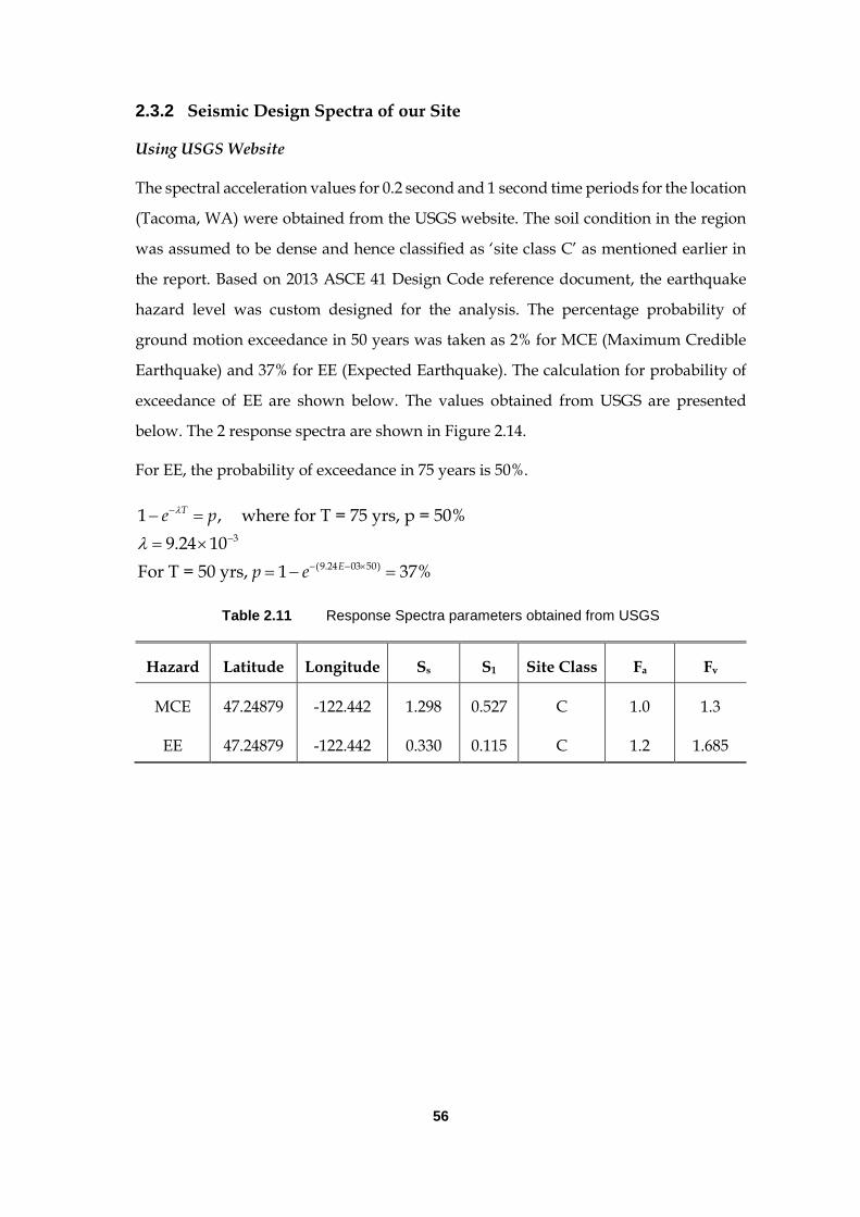
56

2.3.2 Seismic Design Spectra of our Site

Using USGS Website

The spectral acceleration values for 0.2 second and 1 second time periods for the location

(Tacoma, WA) were obtained from the USGS website. The soil condition in the region

was assumed to be dense and hence classified as ‘site class C’ as mentioned earlier in

the report. Based on 2013 ASCE 41 Design Code reference document, the earthquake

hazard level was custom designed for the analysis. The percentage probability of

ground motion exceedance in 50 years was taken as 2% for MCE (Maximum Credible

Earthquake) and 37% for EE (Expected Earthquake). The calculation for probability of

exceedance of EE are shown below. The values obtained from USGS are presented

below. The 2 response spectra are shown in Figure 2.14.

For EE, the probability of exceedance in 75 years is 50%.

3

(9.24 03 50)

1 , where for T = 75 yrs, p = 50%

9.24 10

For T = 50 yrs, 1 37%

T

E

e p

p e

Table 2.11 Response Spectra parameters obtained from USGS

Hazard Latitude Longitude Ss S1 Site Class Fa Fv

MCE 47.24879 -122.442 1.298 0.527 C 1.0 1.3

EE 47.24879 -122.442 0.330 0.115 C 1.2 1.685

57

MCE EE

Figure 2.14 Response Spectra obtained for our site from USGS website for MCE and EE

Using PEER Ground Motion Database

The values of S1 and Sd obtained from USGS were input into PEER Ground Motion

Database to obtain the scaled design spectra. The target spectrum was generated based

on ASCE Spectrum. The long period transition period (TL) was taken as 6 second as

obtained from USGS website. The values for the site coefficients Fa (Short period range)

and Fv (long period range) were obtained from MCEER/ATC-49(Part 1) Table 3.4.2.3-1

and 2. The Sds and Sd1 values were calculated as follows.

MCE – 2% in 50 years

Fa = 1

Fv = 1.3

Sds = Ss *Fa= 1.298 * 1= 1.298

Sd1 = S1*Fv= 0.527 * 1.3= 0.685

EE – 37% in 50 years

Fa = 1.2 (Interpolated)

Fv = 1.685 (interpolated)

Sds = Ss *Fa= 0.330 * 1.2 = 0.396 g

Sd1 = S1*Fv= 0.115 * 1.685 = 0.193 g

58

MCE EE

Figure 2.15 Response Spectra in PEER Ground motion Database

2.3.3 Ground Motion Selection

Ground motion selection is one of the most important factors for performing time

history analysis and should not be affected by performance characteristics of the

structure. In the present project the ground motions were selected and scaled in PEER

ground motion database.

2.3.4 Development of Response Spectra and Scaling of Ground Motions

The selected ground motions are scaled w.r.t. MCE and EE level spectra according to

MCEER ATC 49 such that

The mean response spectra never lies below 15% of the design spectra for any

period and,

The average ratio of the mean spectra and the target spectra shall not be less than

unity over the period range of significance.

So these two considerations were made while scaling the ground motions to the target

spectrum in PEER database.

After generating the target spectrum with the above values in PEER Ground Motion

Database, a magnitude range of 6.5-8.5 was selected to generate a list of ground motions

in that range. The period of interest was given between 0.2 and 1.8 s which more or less

capture the first 30 modes of the structure to ensure better match between the response

spectra of the selected GMs and the target spectra. 3 locations were selected from the

list of records each for MCE and EE hazard level to scale the target spectrum using the

59

average of their spectral acceleration curves. The curves of the selected locations were

chosen so that the scaling factor would be 2.5 or less. In addition, the ground motions

already present in the NONLIN database was selected, so that scaling will be easy for

the time history analysis in NONLIN program, the result of which is presented in the

succeeding sections. The resultant ground motion average spectra is compared with the

target spectra in Figure 2.16 to Figure 2.18. The list of ground motions and their

corresponding scale factors are presented in Table 2.12. It can be seen from the Figures

that the mean response spectra of the selected ground motions after scaling never falls

below 0.85 times the target spectra and also the ratio of the mean spectra to the target

spectra is approximately 1.02 for both MCE and EE. Thus, both the considerations of

ATC 49 are duly met.

MCE EE

Figure 2.16 Resultant ground motion spectra compared with target spectra in PEER

Figure 2.17 Comparison of the mean response spectra of the selected GMs with the target spectra and 85% of target spectra at EE

60

Figure 2.18 Comparison of the mean response spectra of the selected GMs with the target spectra and 85% of target spectra at MCE

Table 2.12 Scaled ground motions selected from PEER Database

No Ground Motion NGA# Scale M Year Station

MC

E

1 Cape Mendocino 828 1.0 7.01 1992 Petrolia

2 North Ridge 960 1.0 6.69 1994 Canyon Country

-W Lost Cany

3 Loma-Prieto 753 1.0 6.93 1989 Corralitos

EE

1 North Ridge 1048 0.3788 6.69 1994 North Ridge 17645

Saticoy St

2 Imperial Valley 181 0.4671 6.53 1979 El-Centro #6

3 Kobe Japan 1116 0.7236 6.90 1995 Shin-Osake

2.4 DEVELOPMENT OF SDOF MODEL

A simple elastic SDoF analysis of the bridge was performed using the program

NONLIN, in which a lumped mass model was developed with the entire mass of the

superstructure and the piers lumped at the node. The piers of the bridge were modeled

as a single column with effective stiffness values in longitudinal and transverse

directions (local) and global X (chord) and Y (radial) directions. The primary objective

to carry out this simplified analysis was to get a preliminary idea about the response of

the bridge along two principal directions, when subjected to different level of ground

motions scaled with the design spectra of our site. The maximum resultant forces of the

piers in both strong and weak directions can also be obtained from this simplified

analysis.

61

2.4.1 Modeling Assumptions

Elastic analysis of the bridge was performed using NONLIN software with a simple

SDoF model in which representative mass and stiffness was assigned to evaluate its

performance in two orthogonal directions. The scaled ground motions were used for

analysis and the maximum resultant forces are reported. The modeling assumptions are

presented as follows:

Mass

As presented earlier in this Chapter, close to 80 modes of vibration are necessary to

entirely capture the overall response of the structure. The following assumptions were

made to consider the mass of structure in local directions (longitudinal and transverse)

and in the two orthogonal directions (chord and radial).

Local Directions: The mass lumped at the node of the SDoF model is the weight

of the superstructure and part of the weight of the participating piers based on

their participation in the respective directions. The masses considered in the

SDoF model in the longitudinal and transverse directions as shown in Section

2.2.4 is 16011.2 and 15711.8 kips, respectively.

Global Directions: The mass lumped at the node of the SDoF model is the weight

of the superstructure and half the weight of the piers, which is 18271.2 kips,

active in both the principal directions along global X and Y.

Stiffness

It is very difficult to characterize the bridge response with a single value of stiffness and

therefore the method 2 presented in Section 2.2.4 and Section 2.2.5 was used to calculate

the bridge lateral stiffness along local ( longitudinal and transverse) and global (chord

and radial) directions, respectively. Therefore, the key assumptions related to stiffness

of the bridge are as follows:

The stiffness of the bridge was calculated along the local and global directions

of bridge both analytically and based on the displacement recorded by applying

unit load in SAP 2000 program.

Local Directions: The values of the equivalent bridge stiffness in the transverse

and longitudinal directions are 28793 kips/feet and 8484 kips/feet, respectively.

62

Global Directions: The values of the equivalent bridge stiffness in the chord (X)

and radial (Y) directions are 10331 kips/feet and 29521 kips/feet, respectively.

Damping

The value of damping used for SDoF analysis was 5% of critical damping, which is

typical for concrete bridges.

2.4.2 Analysis Procedure

A series of time history analysis was performed in NONLIN program using the

simplistic SDoF model of the concerned bridge as described in the preceding sections.

The ground motions selected are scaled according to two seismic hazard levels as

described in Section 2.3.2. The elastic dynamic analysis was performed for the principal

directions, longitudinal and transverse direction (local X and Y), chord and radial

direction (global X and Y) which are corresponding to the weak and strong directions

of the piers respectively. In all there were twelve ground motions (6 for EE and 6 for

MCE) and so, in total, 48 time history analysis were run, 12 along each of the four

directions as described above.


The results of the time history analysis considering simplified elastic linear SDoF model

are presented in Table 2.13. Expected earthquakes has lesser demand on the structure

and hence impose smaller displacement on the piers as compared to the maximum

considered earthquake which impose a demand about 3 times of that of EE as far as

displacements and shear forces are concerned in both transverse and longitudinal

direction. This comes from the difference in response spectra itself. The spectral

acceleration of MCE at short period was 1.298g which is 3.3 times the spectral

acceleration at same period for EE and hence the difference in demands between MCE

and EE is justified.

63

Table 2.13 Results of time history analysis in NONLIN using elastic linear SDoF models along local directions (longitudinal and transverse)

Hazard Level

Ground Motion

Longitudinal Transverse Maximum

Shear (kips)

Disp. (feet)

Shear (kips)

Disp. (feet)

Shear (kips)

Disp (feet)

MC

E

NGA 753-FN 2108.23 .2485 6866.14 .2385

Lo

ng

7496.66 0.8464 NGA 753-FP 5494.80 .6477 21294.58 .7396

NGA 828-FN 3475.63 .4097 19715.00 .6847

NGA 828-FP 7181.12 .8464 20814.34 .7229

Tra

ns

21294.5 0.7396 NGA 960-FN 7496.66 .6738 8520.73 .2959

NGA 960-FP 3135.31 .3696 6486.10 .2253

EE

NGA 181-FN 2349.51 .2769 6424.55 .2231

Lo

ng

3669.45 0.4325 NGA 181-FP 2807.07 .3309 3862.65 .1342

NGA 1048-FP 2373.31 .2797 2698.36 .0397

NGA 1048-FP 2132.93 .2514 4507.14 .1565

Tra

ns

7075.49 0.2457 NGA 1116-FP 1748.23 .2061 4438.99 .1542

NGA 1116-FP 3669.45 .4325 7075.49 .2457

Table 2.14 Results of time history analysis in NONLIN using elastic linear SDoF models along global directions (X and Y)

Hazard Level

Ground Motion Global X Global Y Maximum

Shear (kips)

Disp. (feet)

Shear (kips)

Disp. (feet)

Shear (kips)

Disp (feet)

MC

E

NGA 753-FN 2757.22 .2669 7356.05 .2492

X

8426.75 .8157

NGA 753-FP 6905.20 .6684 20409.00 .6913

NGA 828-FN 4165.44 .4032 18875.97 .6394

NGA 828-FP 8426.75 .8157 20743.91 .7027

Y

20743.91

.7027

NGA 960-FN 6136.84 .5940 9195.69 .3115

NGA 960-FP 3801.43 .3680 7144.12 .2420

EE

NGA 181-FN 2950.20 .2856 6803.53 .2305

X

4051.63 .3922

NGA 181-FP 3160.45 .3059 4206.73 .1425

NGA 1048-FP 3048.14 .2950 3168.14 .1073

NGA 1048-FP 3105.05 .3006 5007.08 .1696

Y

6803.53 .2305

NGA 1116-FP 2296.96 .2223 5644.35 .1912

NGA 1116-FP 4051.63 .3922 6282.22 .2128

64


Multimode analysis of the bridge is carried out in SAP 2000 program considering all the

modes which contribute significantly to the overall behaviour of the structure. The

response spectra for our site (Tacoma) has been obtained for both design earthquake

(DE) and maximum credible earthquake (MCE). A suite of ground motions is selected

for time history analysis and scaled by comparing their corresponding response spectra

to the design spectra for our site. Further, a simplified single degree of freedom (SDoF)

model of the bridge was developed in NONLIN software to examine its behaviour and

compared with the response obtained in SAP 2000 program. The following observations

were made during the analysis process.

83 Eigen values were needed to capture 100% mass participation in both

translation and rotation along all the three directions.

The first three natural periods coming from the modal analysis are 1.54 s, 0.88 s

and 0.75 s, respectively.

First mode is primarily associated with translation in longitudinal direction

while the second mode is associated with translation in transverse direction. The

third mode is associated with torsion (rotation about vertical axis)

The longitudinal stiffness calculated based on the displacement recorded in the

uniform load method in SAP 2000 program is in good agreement with the value

calculated analytically (9844 kips/feet).

However, the transverse stiffness calculated analytically is much higher because,

it is not correct to calculate the pier stiffness in transverse direction considering

it to be fixed at the base.

Expected earthquakes has lesser demand on the structure and hence impose

smaller displacement on the piers as compared to the maximum considered

earthquake which impose a demand about 3 times of that of EE as far as

displacements and shear forces are concerned in both transverse and

longitudinal direction.

-o-o-o-

65

CHAPTER 3 3. UNIFORM LOAD, DYNAMIC MULTIMODE AND PUSHOVER ANALYSIS

UNIFORM LOAD, DYNAMIC MULTIMODE AND PUSHOVER ANALYSIS

3.1 GENERAL OVERVIEW

The bridge was subjected to a uniform load and the stiffness was calculated according

to uniform load method presented in MCEER/ATC 49 document. The previous chapter

deals with the modal analysis and development of the response spectra for the site. In

this chapter the response of the bridge is obtained by appropriately considering the

effects of all the natural modes of vibration significantly contributing to the overall

response according to multimode analysis. A nonlinear static analysis referred to as

pushover analysis is conducted to find out the force-displacement relationship of the

structure in global coordinate system. Triangular lateral load was applied to an

individual pier and to the entire bridge in both longitudinal and transverse directions.

The lateral load-displacement response and the moment curvature plots of the plastic

hinges developed are presented herein.

3.2 UNIFORM LOAD METHOD

3.2.1 Introduction

As stated previously in Chapter 1, the primary objective of uniform load method is to

determine the displacement demand of the superstructure of the bridge. This method is

based on fundamental mode of vibration in the longitudinal or transverse directions.

66


The uniform load method was performed according to MCEER/ATC-49 section 5.4.2.2.

Unit load was applied laterally to the superstructure along longitudinal and transverse

direction and the maximum displacement was determined, based on which the stiffness

and the corresponding time periods were obtained. The elastic seismic response

demand coefficient was obtained from the MCE and EE response spectrum developed

for the site as presented in Chapter 2 corresponding to the period of the structure in

longitudinal and transverse directions.

STEP 1:-The maximum displacement is obtained by assigning uniform distributed load,

Po of 1 kip/ft on entire superstructure in both local transverse and longitudinal

directions respectively.

Figure 3.1 Distribution of load Po in transverse direction

Figure 3.2 Distribution of load Po in longitudinal direction

67

Figure 3.3 Maximum displacement recorded in transverse direction

Figure 3.4 Maximum displacement recorded in longitudinal direction

STEP 2:- Lateral stiffness of the bridge, K is calculated from the expression

o

s

s

P LK

v

v

L

max

maxwhere, Maximum value of displacement recorded on either direction

Length of the superstructure = 1384 ft

STEP 3:- The dead load, W acting on the superstructure was calculated by the following

equation and the weight of the participating piers was added to the self-weight of the

superstructure to get the total mass.

L

super

super

long super piers long

trans er piers trans

W W x dx

W kips

W W W kips

W W W kips

0

sup

( )

9.3 1384 12871.2

16011.2

18271.2

The calculations are based on the participation of the piers in either direction.

68

STEP 4:- Based on the stiffness and weight calculated in the previous steps, the time

period associated with the longitudinal and transverse vibration was calculated

according to the following expression.

2m

WT

Kg

STEP 5:- From the response spectra curve, the demand coefficient, Cd was obtained

corresponding to the longitudinal and transverse period, based on which the equivalent

static earthquake loading, Pe was calculated.

e d

WP C

L

STEP 6:- Finally, the load Pe was applied to the superstructure and the maximum

displacement, base shear and maximum moments were obtained

Following assumptions were made in the analysis

• The analysis was linear.

• The value for acceleration due to gravity, g is 32.174 ft/s2.

• Since linear elastic analysis was done, the results obtained in this section will be

proportional to those obtained in Chapter 1 due to application of a uniform load of 40

kips/feet.


Summary of the results obtained from the Uniform Load Method as extracted from SAP

2000 program is shown in Table 1.1.

69

Table 3.1 Summary of uniform load method results obtained from SAP 2000

Direction of applied load

Transverse Longitudinal

Max displacement (ft) 0.037 0.144

Lateral Stiffness (kip/ft) 36808.5 9631.17

Time Period (s) 0.78 1.43

Hazard level EE MCE EE MCE

Cd 0.2486 0.8825 0.133 0.47

Pe (kip/ft) 3.281 11.65 1.5386 5.437

Base Shear (kips) 4542.22 16124.33 2129.49 7525.26

Maximum Moment (kips-feet) 5698.64 20234.42 2704.91 9558.44

Max Displacement after Pe (ft) 0.124 0.442 0.228 0.775

The stiffness and the time period values are in close agreement with the modal analysis

results both in transverse and longitudinal direction which further validates the

uniform load method procedure followed in SAP 2000 program. For transverse

direction, corresponding displacements for EE and MCE are 0.124 feet and 0.442 feet

respectively which translates into base shear of 4542.22 kip and 16124.33 kip, and a

maximum bending moment of 5698.64 kip-ft and 20234.42 kip-ft. Similarly, for

longitudinal direction, corresponding displacements for EE and MCE are 0.228 feet and

0.775 feet, respectively which translates into base shear of 2129.49 kip and 7525.26 kip,

and a maximum bending moment of 2704.91 kip-ft and 9558.44 kip-ft, respectively. The

100%-40% combination rule was applied also to uniform load method, so that it can be

compared with the multimode analysis results. The shear force, bending moment,

displacement and axial force at the piers recorded for 40 kips/feet applied to the

superstructure in longitudinal and transverse directions as described in Chapter 1 is

used in this section for the 100-40 combination. Since the analysis is elastic, all the

resultant forces will be Pe/40 times of those presented in Table 1.4 and Table 1.5 of

Chapter 1. The results thus obtained are shown in Table 3.2 to Table 3.5.

70

Table 3.2 Forces, moments and displacements - 100% EE_Trans + 40% EE_long

Piers Shear(kips)

Moment (kips-feet)

Displacement (feet)

Axial force


Left Abut 24.12 258.13 0.00 91.42 0.05 0.14 4.29

Pier 1 0.00 594.34 33906.50 0.00 0.08 0.13 69.74

Pier 2 413.14 621.64 40565.75 23961.84 0.09 0.12 96.86

Pier 3 156.59 513.03 41812.02 12213.71 0.11 0.10 71.41

Pier 4 0.00 562.81 45482.13 0.00 0.12 0.09 41.46

Pier 5 129.03 556.75 44691.50 10063.95 0.11 0.10 91.41

Pier 6 373.50 624.44 40377.43 21663.17 0.09 0.12 113.64

Pier 7 0.00 596.82 33990.18 0.00 0.08 0.13 74.25

Right Abut

24.65 259.10 0.00 91.57 0.05 0.14 4.31

Table 3.3 Forces, moments and displacement - 40% EE_Trans + 100% EE_long

Piers Shear(kips)

Moment (kips-feet)

Displacement (feet)

Axial force


Left Abut 11.16 108.61 0.00 39.89 0.02 0.24 1.81

Pier 1 0.00 263.17 14859.76 0.00 0.04 0.24 36.95

Pier 2 792.89 261.70 17007.09 45987.72 0.04 0.23 41.47

Pier 3 329.23 211.43 16839.31 25679.75 0.05 0.22 43.79

Pier 4 0.00 253.50 19450.54 0.00 0.05 0.22 59.97

Pier 5 316.55 305.01 23042.46 24690.53 0.05 0.22 98.58

Pier 6 769.72 265.98 16274.32 44643.93 0.04 0.23 87.23

Pier 7 0.00 268.07 14969.48 0.00 0.04 0.24 48.24

Right Abut

12.52 111.12 0.00 39.95 0.02 0.24 1.85

71

Table 3.4 Forces, moments and displacements - 100% MCE_Trans + 40% MCE_long


Displacement (feet)

Axial force


Left Abut 85.64 916.51 0.00 324.59 0.19 0.49 15.25

Pier 1 0.00 2110.12 120382.09 0.00 0.29 0.45 247.54

Pier 2 1461.48 2207.17 144031.92 84765.56 0.33 0.41 343.89

Pier 3 553.67 1821.60 148462.91 43186.79 0.41 0.36 253.44

Pier 4 0.00 1998.14 161484.56 0.00 0.44 0.31 146.83

Pier 5 455.85 1976.14 158643.25 35554.65 0.41 0.36 324.03

Pier 6 1320.82 2217.09 143368.95 76607.26 0.33 0.41 403.14

Pier 7 0.00 2118.90 120678.56 0.00 0.29 0.45 263.49

Right Abut

87.49 919.95 0.00 325.11 0.19 0.49 15.30

Table 3.5 Forces, moments and displacements - 40% MCE_Trans + 100% MCE_long


Displacement (feet)

Axial force


Left Abut 39.61 385.54 0.00 141.55 0.08 0.85 6.41

Pier 1 0.00 933.90 52735.02 0.00 0.13 0.83 131.01

Pier 2 2801.70 928.96 60370.89 162498.57 0.14 0.81 147.19

Pier 3 1163.20 750.60 59789.65 90729.77 0.17 0.79 155.16

Pier 4 0.00 899.49 69036.57 0.00 0.18 0.77 211.99

Pier 5 1118.21 1081.23 81705.52 87220.14 0.17 0.79 348.69

Pier 6 2719.59 944.09 57783.29 157736.35 0.14 0.81 308.82

Pier 7 0.00 951.20 53122.94 0.00 0.13 0.83 170.88

Right Abut

44.40 394.39 0.00 141.76 0.08 0.85 6.56

72

3.2.4 Summary

The demand is higher for MCE than EE as expected. The maximum moment, shear and

displacement was observed to be approximately 3.5 times for MCE compared to EE,

similar to the results obtained for simplified SDoF model in NONLIN program as

presented in Chapter 2. The observed maximum displacements are 0.44 feet and

0.78 feet in transverse and longitudinal directions, respectively. Coupling of modes in

orthogonal directions are neglected for the analysis purpose. However, from the results,

it can be seen that there are some traces of coupling between the orthogonal modes

which is because there is some moment and shear generated in the direction orthogonal

to loading.

3.3 DYNAMIC MULTI-MODE ANALYSIS

3.3.1 Introduction

The seismic analysis for the bridge as modeled in SAP 2000 program is done by Dynamic

Multimode method. This method is used to obtain information about the contribution

of each mode towards the motion of the structure. The dynamic multimode behaviour

is investigated based on the participation of various modes. The various mode shapes

and corresponding periods obtained from modal analysis are used. According to

MCEER/ATC 49 report, the number of modes included in the analysis shall be atleast 3

times the number of spans in the model for regular bridges and a total mass

participation of 90%. This is achieved at the 27th mode for the bridge as presented in the

previous chapter.


The response of the structure during a seismic event of MCE and EE level was

determined using the multimode method of analysis. EE and MCE response spectra

corresponding to 5% damping was constructed in Chapter 2. The spectra were assigned

in two principal orthogonal directions, longitudinal and transverse. As suggested in

Article 5.4.2.3 of MCEER ATC 49, the member forces and displacements due to a single

component of ground motion can be estimated by combining the respective response

quantities from the individual modes by Complete Quadratic Combination (CQC)

method. In addition, according to Article 3.6, the maximum force due to two or three

73

orthogonal ground motion components, shall be obtained by the 100%-40%

combination forces due to the individual seismic loads. Thus, in the present project the

modes were combined using CQC method and the directional effects were considered

by 100%-40% rule. Ambient damping of 5% was considered to be typical for concrete

bridges and hence used in the analysis.

The analysis procedure followed in SAP 2000 program is presented as follows:

The load case type was defined for response spectra in SAP2000 and calculations

are done based on CQC (Complete Quadratic Combination) rule.

The General Modal Combination (GMC) values for f1 and f2 are taken as 1 and

0 respectively, where f1 and f2 are frequencies that define the rigid response

content of the ground motion

The default value of f2 is taken as 0 indicating infinite frequency. For the default

value, GMC method gives results similar CQC method.

The response spectra for EE and MCE earthquakes are defined in SAP 2000

program.

The load combinations are calculated by 100%-40% rule as specified in MCEER

ATC 49. Based on this, for ‘Absolute’ Directional Combination the scale factor is

taken as 1. The SRSS directional combination was not considered.

The structure is analyzed for these load combinations of EE and MCE, in both

transverse and longitudinal directions.

74

Figure 3.5 Response Spectrum function for MCE

Figure 3.6 Response Spectrum function for EE

75

Figure 3.7 Load case 100 MCE - Long + 40 MCE - Trans

Figure 3.8 Load case 100 MCE - Trans + 40 MCE - Long

76

Figure 3.9 Load case 100 EE - Long + 40 EE - Trans

Figure 3.10 Load case 100 EE - Trans + 40 EE - Long

77


The 2D stick model of the bridge was subjected to Expected Earthquake and Maximum

Considered Earthquake loads in SAP2000 program. The response of bridge was

computed in terms of joint displacement, shear force and bending moments for different

members. It should be noted that the effect of the dead load have been tabulated

separately in Table 3.6.Table 3.7 to Table 3.10 contain the resultant forces, Table 3.11 and

Table 3.12 presented the resultant displacements only due to seismic loading. The

discussion of the results in terms of force and displacement demands are presented

herein.

Table 3.6 Forces and moments under dead load

Forces and moments in Substructure

Longitudinal direction

Transverse direction Axial force

(kip) Support location

Shear

(kip)

Moment

(kip ft)

Shear

(kip)

Moment

(kip ft)

Left abutment 637.2 0 0.142 13.25 0

Pier 1 0 144.46 0.245 0 1818.00

Pier 2 4.85 181.49 0.247 248.08 1557.00

Pier 3 1.21 125.89 0.801 094.16 1623.19

Pier 4 0 172.58 0.840 0 1623.18

Pier 5 0 122.59 0.840 0 1623.18

Pier 6 7.692 177.98 0.310 446.11 1557.00

Pier 7 0 142.35 0.246 0 1818.78

Right abutment 637.196 0 0.143 13.4 0

78

Table 3.7 Forces and moments for EE - 100% EE_Long + 40% EE_Trans

Pier No.

Longitudinal Transverse Axial Force

(Kip) Shear

(Kip)

Moment

(Kip-ft)

Shear

(Kip)

Moment

(Kip-ft)

Abutment 1 8.135 344.809 168.917 7308.002 33.398

Pier 1 275.635 10352.7729 643.082 32312.918 15.568

Pier 2 375.995 19503.749 657.851 35476.902 9.087

Pier 3 196.118 10108.8446 650.734 44985.486 18.234

Pier 4 122.583 5739.428 761.313 52667.77 7.330

Pier 5 196.176 10110.4316 650.753 44987.154 18.236

Pier 6 376.003 19503.5557 657.840 35476.85 9.084

Pier 7 275.713 10355.72 643.078 32313.08 15.566

Abutment 2 8.134 344.6982 168.921 7308.2031 33.416

Table 3.8 Forces and moments for EE - 100% EE_Trans + 40% EE_Long

Pier No.


(Kip) Shear

(Kip)

Moment

(Kip-ft)

Shear

(Kip)

Moment

(Kip-ft)

Abutment 1 9.311 402.5184 128.528 5559.594 32.879

Pier 1 391.975 14722.46 447.424 22348.29 25.359

Pier 2 656.854 35290.76 444.287 23835.345 13.715

Pier 3 367.409 20216.915 387.613 25900.009 28.402

Pier 4 306.358 14478.88 304.634 21074.615 2.936

Pier 5 367.433 20218.201 387.649 25902.866 28.403

Pier 6 656.893 35292.95 444.364 23839.715 13.714

Pier 7 391.972 14722.38 447.513 22353.22 25.359

Abutment 2 9.310 402.4965 128.504 5560.6226 32.895

79

Table 3.9 Forces and moments for MCE - 100% MCE_Long + 40% MCE_Trans

Pier No.


(Kip) Shear

(Kip)

Moment

(Kip-ft)

Shear

(Kip)

Moment

(Kip-ft)

Abutment 1 28.907 1225.3025 600.342 25973.152 118.613

Pier 1 993.817 37327.497 2281.680 114662.0898 55.595

Pier 2 1322.079 68960.6176 2330.013 125658.266 32.422

Pier 3 699.845 35743.099 2301.748 159105.412 64.916

Pier 4 437.150 20518.7347 2692.952 186279.955 26.289

Pier 5 700.052 35748.710 2301.818 159111.3039 64.924

Pier 6 1332.109 68959.936 2329.973 125658.03 32.413

Pier 7 994.1 37338.153 2281.664 114662.62 55.589

Abutment 2 28.906 1224.8778 600.358 25973.854 118.677

Table 3.10 Forces and moments for MCE - 100% MCE_Trans + 40% MCE_Long

Pier No.


(Kip) Shear

(Kip)

Moment

(Kip-ft)

Shear

(Kip)

Moment

(Kip-ft)

Abutment 1 8.135 344.6892 168.917 7308.002 33.398

Pier 1 1413.287 53082.645 1587.481 79300.82 90.609

Pier 2 2325.673 124775.2836 1573.527 84425.745 48.969

Pier 3 1309.983 71479.3927 1371.968 91656.6892 101.202

Pier 4 1092.524 51280.258 1077.564 74358.529 10.529

Pier 5 1310.067 71483.940 1372.099 91666.7887 101.203

Pier 6 2325.81 124783.011 1573.801 84441.21 48.966

Pier 7 1413.278 53082.3679 1587.797 79318.310 90.609

Abutment 2 8.134 344.6892 168.921 7308.2031 33.416

80

Table 3.11 Displacement under Expected Earthquake

Location

100% EE_Long + 40% EE_Trans

100% EE_Trans + 40% EE_Long

Long (ft) Trans (ft) Long (ft) Trans (ft)

Left Abutment 0.0433 0.1095 0.0333 0.1813

Pier 1 0.0814 0.1053 0.0565 0.1813

Pier 2 0.0859 0.0975 0.0579 0.1766

Pier 3 0.1252 0.0852 0.0729 0.1721

Pier 4 0.1463 0.066 0.0586 0.1650

Pier 5 0.1252 0.0852 0.0729 0.1722

Pier 6 0.0859 0.0975 0.0579 0.1766

Pier 7 0.0814 0.1053 0.0565 0.1813

Right Abutment 0.0433 0.1095 0.0333 0.1837

Table 3.12 Displacement under Maximum Credible Earthquake

Location

100% MCE_Long + 40% MCE_Trans

100% MCE_Trans + 40% MCE_Long

Long (ft) Trans (ft) Long (ft) Trans (ft)

Left Abutment 0.1541 0.3873 0.0433 0.1095

Pier 1 0.2886 0.3723 0.2003 0.6410

Pier 2 0.3044 0.3447 0.2050 0.6245

Pier 3 0.4428 0.3013 0.2578 0.6068

Pier 4 0.5174 0.2335 0.2070 0.5835

Pier 5 0.4428 0.3014 0.2578 0.6087

Pier 6 0.3044 0.3447 0.2051 0.6426

Pier 7 0.2886 0.3723 0.2003 0.6411

Right Abutment 0.1541 0.3873 0.0433 0.1095

The following observations are made:

i. When the bridge is tested under pure dead load very large axial forces but small

shear and moment values are obtained.

ii. On application of Expected Earthquake, the axial force and shear values are

small but large moments are obtained in the piers as expected.

iii. As for Maximum Credible Earthquake load, very large shear and moment values

are observed compared to expected earthquake due to higher demand.

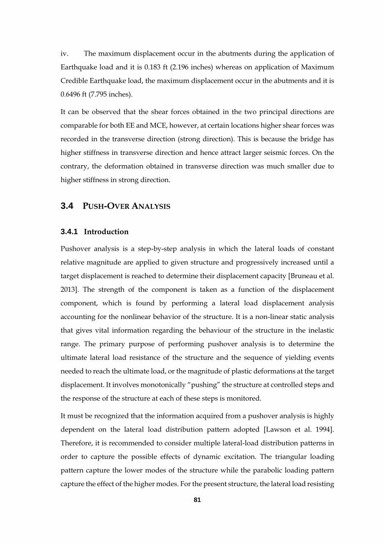
81

iv. The maximum displacement occur in the abutments during the application of

Earthquake load and it is 0.183 ft (2.196 inches) whereas on application of Maximum

Credible Earthquake load, the maximum displacement occur in the abutments and it is

0.6496 ft (7.795 inches).

It can be observed that the shear forces obtained in the two principal directions are

comparable for both EE and MCE, however, at certain locations higher shear forces was

recorded in the transverse direction (strong direction). This is because the bridge has

higher stiffness in transverse direction and hence attract larger seismic forces. On the

contrary, the deformation obtained in transverse direction was much smaller due to

higher stiffness in strong direction.

3.4 PUSH-OVER ANALYSIS

3.4.1 Introduction

Pushover analysis is a step-by-step analysis in which the lateral loads of constant

relative magnitude are applied to given structure and progressively increased until a

target displacement is reached to determine their displacement capacity [Bruneau et al.

2013]. The strength of the component is taken as a function of the displacement

component, which is found by performing a lateral load displacement analysis

accounting for the nonlinear behavior of the structure. It is a non-linear static analysis

that gives vital information regarding the behaviour of the structure in the inelastic

range. The primary purpose of performing pushover analysis is to determine the

ultimate lateral load resistance of the structure and the sequence of yielding events

needed to reach the ultimate load, or the magnitude of plastic deformations at the target

displacement. It involves monotonically “pushing” the structure at controlled steps and

the response of the structure at each of these steps is monitored.

It must be recognized that the information acquired from a pushover analysis is highly

dependent on the lateral load distribution pattern adopted [Lawson et al. 1994].

Therefore, it is recommended to consider multiple lateral-load distribution patterns in

order to capture the possible effects of dynamic excitation. The triangular loading

pattern capture the lower modes of the structure while the parabolic loading pattern

capture the effect of the higher modes. For the present structure, the lateral load resisting

82

system of the bridge (piers) were subjected to triangular load pattern and the response

was studied in details. In our case, out of the various components of the bridge, the

columns/piers designed are considered to be the weakest out of the lot and are thus

checked for their inelastic behavior under lateral loading. The analysis is performed on

individual pier in both longitudinal and transverse direction separately.

Section ATC-C5.4.3, states that the analysis determines the component which reaches

its inelastic deformation capacity first and the corresponding displacement for the

maximum allowable deformation defines the maximum displacement capacity.

Damages can be of various sorts, one of them being plastic hinge rotation. A plastic

hinge, in effect is defined as the part of an element which deforms inelastically as a result

of plastic bending at that point.

3.4.2 Description of Model

According to MCEER/ATC 49 Report, the displacement capacity verification analysis

(pushover analysis) shall be applied to the individual piers to determine the lateral load

displacement behaviour of the pier. The capacity evaluation was performed on

individual piers in the longitudinal and transverse directions separately. The pushover

response of the entire structure was also evaluated and presented in detail.

The model of the bridge developed in SAP 2000 program was used for this purpose. A

six member model is generated, with the top member representing the rigid link and

the bottom most member for the foundation. Four elements were used to model the pier,

to take into account the various cross-sections and reinforcement detailing. The

reinforcement and concrete detailing is imbibed into the structure based on the design

details presented in FHWA Design Example 5 and shown in Figure 3.11 and Figure 3.12.

The pushover model is as shown in the Figure 3.13 below.

83

Figure 3.11 Column cross-section at base

Figure 3.12 Column reinforcement details

84

Figure 3.13 Pushover Model of the 70 feet pier

3.4.3 Plastic Hinge Model

A variety of plastic hinge properties are available in SAP 2000 program. The fiber PMM

hinge was selected to be used for the present project as it is expected to give more

realistic results. This hinge is more “natural” than the Coupled PMM hinge, since it

automatically accounts for axial force-moment interaction, changing moment-rotation

curve, and plastic axial strain.

The Fiber P-M2-M3 (Fiber PMM) hinge models the axial behavior of a number of

representative axial “fibers” distributed across the cross section of the frame element.

Each fiber has a location, a tributary area, and a stress-strain curve. Axial force (P), major

axis moment (M2) and minor axis moment (M3) are calculated by numerically

combining the axial stresses. Similarly, the axial strains of each fiber element are

computed from the axial deformation (U1) and the corresponding rotations, R2 (major

axis) and R3 (minor axis). The nonlinear stress-strain properties of the individual fibers

are presented in the succeeding sections.

3.4.4 Non-linear models for pushover analysis

The reinforcement detailing was done using the Section Designer property of SAP 2000

program. Both the longitudinal bars and the transverse ties were provided as shown in

Figure 3.14 and Figure 3.15. In section designer the section was sub divided into various

fibers with 16 fibers along 2 axis and 90 fibers along 3 axis thus ensuring that each of the

fibers passes through one reinforcement bars in either directions as shown in Figure 3.16

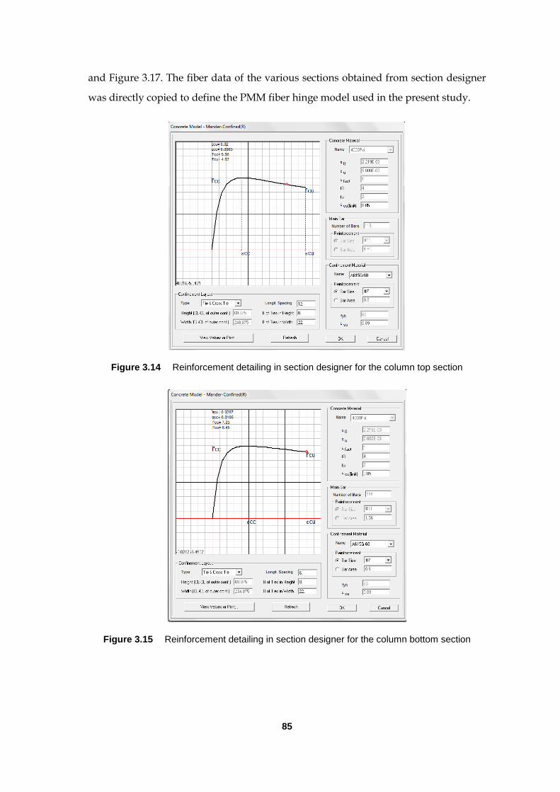
85

and Figure 3.17. The fiber data of the various sections obtained from section designer

was directly copied to define the PMM fiber hinge model used in the present study.

Figure 3.14 Reinforcement detailing in section designer for the column top section

Figure 3.15 Reinforcement detailing in section designer for the column bottom section

86

Figure 3.16 Fiber model of column top in section designer

Figure 3.17 Fiber model of column base in section designer

Bilinear model

A simplified stress-strain model was used to incorporate the non-linear material

behaviour for both concrete and rebar. Perfectly bilinear behavior is assumed for

pushover analysis as shown in Figure 1.8 to Figure 3.21.

Figure 3.18 Bilinear Stress strain model of concrete

87

Figure 3.19 Non-linear material property of concrete

Figure 3.20 Bilinear Stress strain model of rebar

Figure 3.21 Material Property input in SAP 2000

-80

-60

-40

-20

0

20

40

60

80

-0.24 -0.12 0 0.12 0.24

Str

ess (

ksi)

Strain

88

Plastic Hinge Definition

The definition of the plastic hinge at the top of the pier is shown in Figure 3.22. The

fibers created at the section designer was copied to the fiber hinge as shown in Figure

3.23. The plastic hinge definition in the other locations are similar to the one shown in

Figure and hence not shown separately. Shear hinge was not added to the members as

it was checked manually that the shear capacity of the section won’t be reached before

reaching the maximum flexural capacity. Hence, only flexural hinges were considered.

Figure 3.22 Plastic hinge definition in SAP 2000 program at pier bottom

Figure 3.23 Fiber hinge model in SAP 2000

89


The load patterns that are needed for the pushover analysis include the gravity load that

may be acting on the structure before the lateral seismic loads are applied [CSI 2009]

and the lateral loads that will be used to push the structure in the principal directions.

In SAP 2000 program a nonlinear load case is required to be defined and run in sequence

with the lateral pushover load case. Dead load was used in the present model to define

the initial static non-linear load at zero step and the lateral pushover load was assumed

to start from this case. The gravity load coming from the deck was applied as a point

load at the top of the pier. The pushover load case was applied in a displacement

controlled mode a pre-determined target displacement set at 2 feet. Triangular loading

pattern was used to study the pushover behaviour of the bridge as shown in Figure 3.24.

For the individual piers load was applied in local directions to investigate the behaviour

of the piers in longitudinal and transverse directions. However, for the pushover

analysis of the entire bridge the load is applied in global directions to study its

behaviour in radial and chord directions.

Figure 3.24 Triangular loading pattern used in SAP 2000 program

90

Figure 3.25 Typical pushover load case in SAP 2000 program

For the individual piers, the displacement monitored is the displacement of the node

located at the top of the respective piers, while for the pushover analysis of the entire

bridge the displacement of the center of the superstructure is monitored.

Plastic Hinge Length

The calculation of the plastic hinge length and the plastic rotation capacity was carried

out in accordance with the Article 7.8.6 of MCEER/ATC 49 document.

For life Safety Performance,

The plastic rotational capacity is determined by the following equation:

p = 0.11*𝐿𝑝

𝐷′∗ (𝑁f)-0.5 radians (ATC 49 – 7.8.6.1-1)

Where

Nf = Number of cycles of loading expected at the maximum displacement amplitude=

3.5 (Tn)-1/3

Lp = Effective plastic hinge length = 0.08 ∗𝑀

𝑉+ 4400 𝐸𝑌𝐷𝑏

D’ = center-to-center distance between the extreme reinforcement on opposite faces of

the member

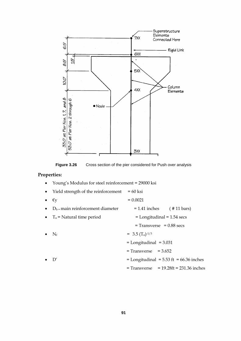
91

Figure 3.26 Cross section of the pier considered for Push over analysis

Properties:

Young’s Modulus for steel reinforcement = 29000 ksi

Yield strength of the reinforcement = 60 ksi

€y = 0.0021

Db = main reinforcement diameter = 1.41 inches ( # 11 bars)

Tn = Natural time period = Longitudinal = 1.54 secs

= Transverse = 0.88 secs

Nf = 3.5 (Tn)-1/3

= Longitudinal = 3.031

= Transverse = 3.652

D’ = Longitudinal = 5.53 ft = 66.36 inches

= Transverse = 19.28ft = 231.36 inches

92

Tabulating the above results,

For Triangular Loading Lp (inches) ᶱp (radians)

For the 70 feet tall pier L T

Plastic hinge at the bottom 57.63 0.0548 0.0143

Plastic hinge at the neck 22.167 0.0210 0.0055

Plastic hinge at the top 12.83 0.0122 0.0032

For the 50 feet tall pier

Plastic hinge at the bottom 44.84 0.0427 0.0112

Plastic hinge at the neck 22.38 0.0211 0.0056

Plastic hinge at the top 12.83 0.0122 0.0032

Based on ATC 49-7.8.6.2, for Immediate Use Performance, the maximum rotational

capacity should be limited to 0.01 radians.

Location of Plastic Hinge

For the individual piers, plastic hinges were considered only at the bottom of the

members, as under lateral loading cantilever action is expected, and plastic hinges will

only be formed at the pier bottom. However, while performing pushover analysis of the

entire structure, plastic hinges were initially to be formed at the base of the pier above

the foundation, the neck and at the top of the pier. After the first analysis it was observed

that the plastic moment capacity was not reached at the top and hence the plastic hinge

at the top of the pier was not considered for further analysis.

In SAP 2000, the plastic hinge is assigned at a discrete point. In the present project the

hinges were assigned at a distance Lp/2 from the nodes, where Lp represent the effective

plastic hinge length calculated according to MCEER/ATC 49.

Figure 3.27 Typical plastic hinge assignment at pier bottom in SAP 2000

93

Figure 3.28 Typical plastic hinge assignment at the column neck in SAP 2000


70 feet pier

The 70 feet pier at the middle of the bridge was considered for pushover analysis. It was

subjected to both longitudinal and transverse directions and the behaviour observed is

presented in this section.

Transverse

The deflected shape of the 70 feet individual pier during pushover analysis in transverse

direction is shown in Figure 3.29. The transverse shear is transferred in the SAP 2000

model and hence the rigid link connecting the pier to the superstructure does not move

with the pier. However, the pier acts as a simple cantilever with plastic hinges formed

only at the bottom. The lateral force-displacement relationship of the individual 70 feet

pier in transverse direction is shown in Figure 3.30. Bilinear load –displacement

relationship was observed as the material properties considered for both steel and

concrete was bilinear in nature.

94

Figure 3.29 Typical deflected shape of the 70 feet pier in transverse direction

Figure 3.30 Force displacement relationship of the 70 feet pier in transverse direction

It was observed that the plastic moment capacity of 1.15 X 106 kips/inch was from the

moment rotation plot of the plastic hinge at the bottom of the pier, which was actually

the maximum capacity of the section as observed in section designer which further

validates our definition of plastic hinge. The typical bilinear behaviour of the 70 feet pier

is shown and the stiffness calculated from pushover curve was compared with the one

obtained in Chapter 2 analytically in succeeding section.

0

500

1000

1500

2000

2500

0 5 10 15 20 25

La

tera

l F

orc

e (

kip

s)

Displacement (inches)

95

Figure 3.31 Moment rotation plot of the plastic hinge at the bottom of the 70 feet pier in transverse direction

From the moment rotation plot, it can be seen that the plastic moment capacity of the

pier in the transverse direction is Mp = 1.15 * 106 kips-inches.

So based on the plastic moment capacity, the maximum shear reached in the pier section

considering cantilever action can be calculated according to the equation pV M L

which comes out to be approximately 1379 kips. The shear strength provided by the

concrete alone in the transverse direction was 2229 kips as reported in the FHWA

Design Example 5, which is much higher than the maximum shear reached. Also, it must

be noted that the actual shear capacity of the section at the bottom of the pier will be

even greater than 2229 kips due to the shear strength of the confining steel reinforcement

and hence, it will be much higher than the maximum base shear (2200 kips) observed

during this case.

Therefore, the shear capacity of the section is greater than the maximum base shear

achieved and shear hinging is thus not possible before flexural yielding along transverse

direction at the bottom of the pier. Similar checks were also carried out along

longitudinal and transverse directions at other plastic hinge locations. In all the cases

the shear capacity of the section was observed to be higher than the maximum base

shear and hence our assumption of not considering the shear hinges is validated.

Longitudinal

The deflected shape of the individual pier in longitudinal direction is shown in Figure

3.32. As the pier 4 was sliding in nature along longitudinal direction as described

0

5 105

1 106

1.5 106

0 0.005 0.01 0.015 0.02 0.025

Mo

me

nt

(kip

s-i

nch

es)

Rotation (radians)

96

previously, cantilever action was observed with plastic hinge being developed only at

the bottom of the pier. The lateral force-displacement relationship of the individual 70

feet pier in transverse direction is shown in Figure 3.33. Exactly bilinear load –

displacement relationship was observed as the material properties considered for both

steel and concrete was bilinear in nature.

Figure 3.32 Typical deflected shape of the 70 feet pier in longitudinal direction

Figure 3.33 Force displacement relationship of the 70 feet pier in longitudinal direction

It can be observed that much higher lateral strength was observed in the transverse

direction compared to longitudinal direction, mainly because of higher plastic moment

capacity in transverse direction.

0

200

400

600

800

1000

0 5 10 15 20 25

La

tre

al F

orc

e (

kip

s)


97

Figure 3.34 Moment rotation plot of the plastic hinge at the bottom of the 70 feet pier in longitudinal direction

50 feet pier

The 50 feet pier at the middle of the bridge was considered for pushover analysis. It was

subjected to both longitudinal and transverse directions.

Transverse

Figure 3.35 Force displacement relationship of the 50 feet pier in transverse direction

0

1 105

2 105

3 105

4 105

5 105

0 0.005 0.01 0.015 0.02 0.025

Mo

me

nt

(kip

s-i

nch

es)

Rotation (radians)

0

600

1200

1800

2400

3000

0 5 10 15 20 25

La

tera

l F

orc

e (

kip

s)


98

Figure 3.36 Moment rotation plot of the plastic hinge at the bottom of the 50 feet pier in transverse direction

Longitudinal

Figure 3.37 Force displacement relationship of the 50 feet pier in longitudinal direction

0

5 x 105

1 x 106

1.5 x 106

0 0.007 0.014 0.021 0.028 0.035

Mo

me

nt

(kip

s-i

nch

es)

Rotation (radians)

0

200

400

600

800

1000

0 5 10 15 20 25

La

tre

al F

orc

e (

kip

s)


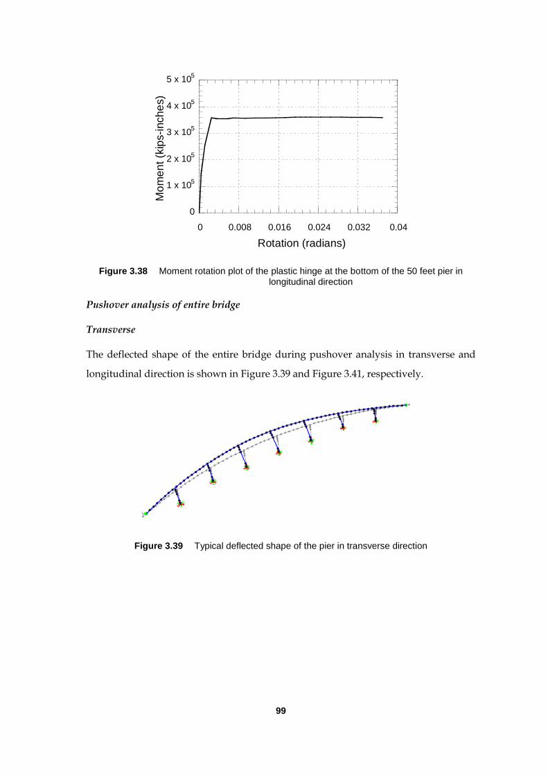
99

Figure 3.38 Moment rotation plot of the plastic hinge at the bottom of the 50 feet pier in longitudinal direction

Pushover analysis of entire bridge

Transverse

The deflected shape of the entire bridge during pushover analysis in transverse and

longitudinal direction is shown in Figure 3.39 and Figure 3.41, respectively.

Figure 3.39 Typical deflected shape of the pier in transverse direction

0

1 x 105

2 x 105

3 x 105

4 x 105

5 x 105

0 0.008 0.016 0.024 0.032 0.04

Mo

me

nt

(kip

s-i

nch

es)

Rotation (radians)

100

Figure 3.40 Force displacement relationship of the bridge in transverse direction

Hinges were observed to be formed at the bottom of the piers initially. The hinges at the

neck were formed at a much higher displacement thereby resulting in much higher

lateral strength in the transverse direction. The moment curvature plots were checked

in SAP 2000 program and it was observed that the maximum plastic capacity of the

section was reached at a plastic rotation of approximately in 0.005 radians, while plastic

hinges were formed at the top only after 0.02 radians approximately.

Longitudinal

Figure 3.41 Typical deflected shape of the pier in longitudinal direction

The lateral force displacement relationship of the entire bridge in longitudinal direction

is presented in Figure 3.42. It can be seen much higher capacity was achieved in the

transverse direction, primarily due to high plastic moment capacity along that direction.

0

5000

10000

15000

20000

25000

30000

0 2 4 6 8

La

tera

l F

orc

e (

kip

s)

Displacement (feet)

101

Figure 3.42 Force displacement relationship of the bridge in longitudinal direction

3.4.7 Comparison of stiffness with analytical results

The initial stiffness obtained from the pushover curves are compared with the stiffness

obtained in Chapter 2 analytically. It can be seen that the values are comparable which

further validates the pushover curves obtained.

Table 3.13 Comparison of stiffness

Stiffness (kips/feet) Longitudinal Transverse

Pushover Analytical Pushover Analytical

70 feet pier 5872 5022 1728 1259

50 feet pier 8100 7841 3375 2983

Stiffness (kips/feet) Chord Radial

Bridge 10500 10331 28889 29521


The results of uniform load method are as follows

A uniform load method of analysis was used to get response of a simplified

model of the bridge was calculated in terms of Max displacement (ft), Lateral

Stiffness (kip/ft) and Time Period (s). these values are observed to be higher

along the longitudinal direction than in transverse

0

1000

2000

3000

4000

5000

0 2 4 6 8

La

tera

l F

orc

e (

kip

s)

Displacement (feet)

102

The stiffness and the time period values are in close agreement with the modal

analysis results both in transverse and longitudinal direction which further

validates the uniform load method procedure followed in SAP 2000 program.

The force, base shear, bending moment and maximum displacement values

calculated along transverse and longitudinal directions for MCE are larger than

those of EE.

In multimode analysis, 27 modes are required to achieve a total mass

participation factor of 90% to comply MCEER/ATC 49 specification according

to which the number of modes included in the analysis shall be atleast 3 times

the number of spans in the model for regular bridges (presented in previous

chapter)

The results of multimode analysis are as follows

When bridge was tested only under dead load, very large axial forces but small

shear and moment values are obtained.

Very large shear and moment values are observed for Maximum Credible

Earthquake in contrast to Expected Earthquake.

The displacement due to MCE is higher than that of EE as expected.

The results of Pushover Analysis are as follows:

For the individual pier model, along both transverse and longitudinal directions,

the shear developed is much greater than the shear capacity of the section and

hence no shear hinge is formed. Hence a flexural plastic hinge is developed at

the base.

The moment curvature plots were checked in SAP 2000 and it was observed that

the maximum plastic capacity of the section was reached.

-o-o-o-

103

CHAPTER 4 4. TIME HISTORY ANALYSIS

TIME HISTORY ANALYSIS


In the previous chapters linear static analysis was carried out which can estimate the

seismic demand of the structure when the material and geometric nonlinearity is not

considered. However, nonlinearity is most likely expected during a seismic event.

Therefore, it is not possible to capture the dynamic behaviour of the structure using

static methods of analysis. Therefore, time history analysis is carried out to investigate

the dynamic response of the bridge both at MCE and EE hazard levels. Initially linear

SDoF analysis was carried out on the bridge to get an idea of its elastic dynamic

response. Both nonlinear SDoF and MDoF analysis was then carried out to capture the

nonlinear dynamic response of the bridge according to MCEER/ATC 49 report. The

nonlinear behaviour of the structural components were included by assigning PMM

fiber hinges in the column elements as described in the previous chapter for pushover

analysis. This chapter deals with the response of the bridge obtained by Nonlinear

Dynamic Analysis. Ground motions scaled to the response spectra for both MCE and

EE hazard levels obtained in Chapter 2, is used for time history analysis. The resultant

forces and the maximum displacements recorded at various hazard levels are tabulated

and compared.

4.2 SELECTED GROUND MOTIONS

According to Cl. 3.4.1 of MCEER ATC 49 report, the design spectra for expected

earthquake (EE) and maximum considered earthquake (MCE) was constructed in USGS

website. Based on this, 3 ground motions were scaled in PEER at each hazard level as

sharathchandra

Highlight

sharathchandra

Highlight

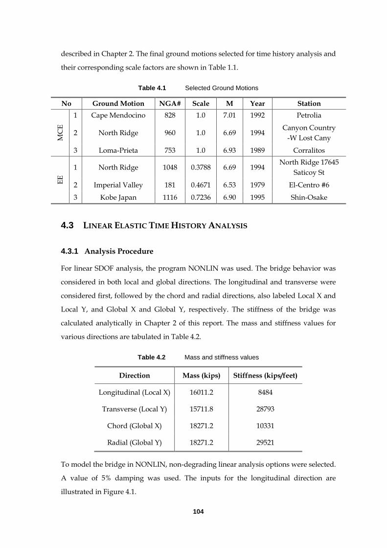
104

described in Chapter 2. The final ground motions selected for time history analysis and

their corresponding scale factors are shown in Table 1.1.

Table 4.1 Selected Ground Motions

No Ground Motion NGA# Scale M Year Station

MC

E

1 Cape Mendocino 828 1.0 7.01 1992 Petrolia

2 North Ridge 960 1.0 6.69 1994 Canyon Country

-W Lost Cany

3 Loma-Prieta 753 1.0 6.93 1989 Corralitos

EE

1 North Ridge 1048 0.3788 6.69 1994 North Ridge 17645

Saticoy St

2 Imperial Valley 181 0.4671 6.53 1979 El-Centro #6

3 Kobe Japan 1116 0.7236 6.90 1995 Shin-Osake

4.3 LINEAR ELASTIC TIME HISTORY ANALYSIS


For linear SDOF analysis, the program NONLIN was used. The bridge behavior was

considered in both local and global directions. The longitudinal and transverse were

considered first, followed by the chord and radial directions, also labeled Local X and

Local Y, and Global X and Global Y, respectively. The stiffness of the bridge was

calculated analytically in Chapter 2 of this report. The mass and stiffness values for

various directions are tabulated in Table 4.2.

Table 4.2 Mass and stiffness values

Direction Mass (kips) Stiffness (kips/feet)

Longitudinal (Local X) 16011.2 8484

Transverse (Local Y) 15711.8 28793

Chord (Global X) 18271.2 10331

Radial (Global Y) 18271.2 29521

To model the bridge in NONLIN, non-degrading linear analysis options were selected.

A value of 5% damping was used. The inputs for the longitudinal direction are

illustrated in Figure 4.1.

105

Figure 4.1 Inputs in NONLIN program for linear analysis along longitudinal direction

A total of 12 ground motions were applied for each of the four directions, totaling in 48

analyses. Three ground motions were considered for both MCE and EE, in two

directions. The ground motions were obtained from the PEER database. The MCE

ground motions obtained from the PEER database had a scale factor of 1.0, while the EE

ground motion scale factors varied. In order to use these ground motions in NONLIN,

the .acc files from PEER were inputted into an excel spreadsheet and the maximum

absolute value was found for each one. Then, this value was multiplied by the scale

factor to get the maximum acceleration in terms of g that would be used for NONLIN.

The ground motions were chosen specifically to match up with the ones already in

NONLIN so that no further inputs would be needed. When inputting the ground

motions for analyses, the motion with the corresponding NGA # was selected and then

the maximum acceleration was specified. The ground motions used, as well as their

PGAs scaled at various hazard levels are listed in Table 4.3.

106

Table 4.3 Scaled PGA (g) of respective GMs

EE MAX SCALED MCE MAX SCALED

181 FN 0.441714 0.206325 753 FN 0.484298 0.484298

181 FP 0.400183 0.186925 753 FP 0.513568 0.513568

1048 FN 0.413276 0.156549 828 FN 0.614812 0.614812

1048 FP 0.422155 0.159912 828 FP 0.629605 0.629605

1116 FN 0.186614 0.135034 960 FN 0.465964 0.465964

1116 FP 0.271347 0.196347 960 FP 0.336958 0.336958

4.3.2 Results

For each ground motion, maximum displacement, and base shear values were obtained

from NONLIN program. The base shear was taken as the maximum spring force from

the output file. These values are shown in Table 4.4.

Table 4.4 Resultant forces and displacements in local directions

Hazard Level

Ground Motion

Longitudinal Transverse Maximum

Shear (kips)

Disp. (feet)

Shear (kips)

Disp. (feet)

Shear (kips)

Disp (feet)

MC

E

NGA 753-FN 2108.23 .2485 6866.14 .2385

Lo

ng

7496.66 0.8464 NGA 753-FP 5494.80 .6477 21294.58 .7396

NGA 828-FN 3475.63 .4097 19715.00 .6847

NGA 828-FP 7181.12 .8464 20814.34 .7229

Tra

ns

21294.5 0.7396 NGA 960-FN 7496.66 .6738 8520.73 .2959

NGA 960-FP 3135.31 .3696 6486.10 .2253

EE

NGA 181-FN 2349.51 .2769 6424.55 .2231

Lo

ng

3669.45 0.4325 NGA 181-FP 2807.07 .3309 3862.65 .1342

NGA 1048-FP 2373.31 .2797 2698.36 .0397

NGA 1048-FP 2132.93 .2514 4507.14 .1565

Tra

ns

7075.49 0.2457 NGA 1116-FP 1748.23 .2061 4438.99 .1542

NGA 1116-FP 3669.45 .4325 7075.49 .2457

107

Table 4.5 Resultant forces and displacements in global directions

Hazard Level

Ground Motion Global X Global Y Maximum

Shear (kips)

Disp. (feet)

Shear (kips)

Disp. (feet)

Shear (kips)

Disp (feet)

MC

E

NGA 753-FN 2757.22 .2669 7356.05 .2492

X

8426.75 .8157 NGA 753-FP 6905.20 .6684 20409.00 .6913

NGA 828-FN 4165.44 .4032 18875.97 .6394

NGA 828-FP 8426.75 .8157 20743.91 .7027

Y

20743.9 .7027 NGA 960-FN 6136.84 .5940 9195.69 .3115

NGA 960-FP 3801.43 .3680 7144.12 .2420

EE

NGA 181-FN 2950.20 .2856 6803.53 .2305

X

4051.63 .3922 NGA 181-FP 3160.45 .3059 4206.73 .1425

NGA 1048-FP 3048.14 .2950 3168.14 .1073

NGA 1048-FP 3105.05 .3006 5007.08 .1696

Y

6803.53 .2305 NGA 1116-FP 2296.96 .2223 5644.35 .1912

NGA 1116-FP 4051.63 .3922 6282.22 .2128

Linear elastic time history analysis was also carried out in SAP 2000 program and the

results obtained are tabulated in Table 4.6 and Table 4.7. The comparison of the

maximum values obtained from elastic analysis in SAP 2000 and NONLIN is presented

in Table 4.8. The values obtained from NONLIN were different from those obtained

from SAP 2000. There is a difference of about 20% in the results with the values obtained

from SAP2000 being higher.

Table 4.6 Resultant forces and displacements obtained in linear elastic time history analysis in SAP 2000 program at EE

Load Case Moment (kips-feet)) Shear (kips)

Displacement (feet)

Trans Long Long Trans Long Trans

IV_FNU1+FPU2_EE 12916.67 22408.33 637.30 2058.00 0.18 0.35

IV_FNU2+FPU1_EE 78825.00 29700.00 645.90 1161.00 0.24 0.20

NR_FNU1+FPU2_EE 64891.67 39416.67 666.40 909.00 0.32 0.16

NR_FNU2+FPU1_EE 100000.00 17691.67 483.00 1639.00 0.14 0.27

KJ_FNU1+FPU2_EE 113333.33 32416.67 547.00 1800.00 0.26 0.31

KJ_FNU2+FPU1_EE 127500.00 42416.67 672.00 1950.00 0.34 0.34

108

Table 4.7 Resultant forces and displacements obtained in linear elastic time history analysis in SAP 2000 program at MCE

Load Case Moment (kips-feet)) Shear (kips)

Displacement (feet)


NR_FNU1+FPU2_MCE 227500.00 77416.67 1300.00 3820.00 0.62 0.63

NR_FNU2+FPU1_MCE 230833.33 83090.33 1450.00 3690.00 0.67 0.63

LM_FNU1+FPU2_MCE 259166.67 152500.00 2730.00 3790.00 0.12 0.65

LM_FNU2+FPU1_MCE 406666.67 68583.33 1820.00 5946.00 0.56 1.05

CM_FNU1+FPU2_MCE 495833.33 124166.67 2400.00 7810.00 1.16 1.33

CM_FNU2+FPU1_MCE 492500.00 133333.33 2850.00 7170.00 1.08 1.29

Table 4.8 Comparison of maximum values recorded for linear time history analysis in SAP 2000 and NONLIN

Hazard

Level

Base Shear (kips) Displacement (feet)

Long Trans Long Trans

NON SAP NON SAP NON SAP NON SAP

MCE 8426.75 12130 20743.9 32080 0.81 1.16 0.70 1.33

EE 4051.63 5731 6803.53 10250 0.39 0.34 0.23 0.35

4.3.3 Summary

As observed from the results of linear elastic SDoF analysis in NONLIN expected

earthquakes has lesser demand on the structure and hence impose smaller displacement

on the piers as compared to the maximum considered earthquake which impose a

demand about 3 times of that of EE as far as displacements and shear forces are

concerned in both local (longitudinal and transverse) and global (chord and radial)

directions. This comes from the difference in response spectra itself. The spectral

acceleration of MCE at short period was 1.298g which is 3.3 times the spectral

acceleration at same period for EE and hence the difference in demands between MCE

and EE is justified.

sharathchandra

Highlight

109

4.4 NON LINEAR DYNAMIC TIME HISTORY ANALYSIS

4.4.1 Introduction

Nonlinear Dynamic Analysis gives the displacement of each node of the structure, thus

giving a good approximation about the response of a structure towards an earthquake.

Ground motions for different locations are fed into NONLIN and SAP2000 program for

SDoF and MDoF, respectively and the structure is analyzed for each. In order to ensure

that the results obtained for each GM are stable, GMs for three different locations are

chosen and the results are compared. A nonlinear mathematical model of bridge has

been defined for the analysis and analysis has been performed for different load cases

to obtain the response quantities.

4.4.2 Code Specification

As mentioned in MCEER ATC 49 under section 5.1.2, “When required the Seismic

Design and Analysis Procedure use the following seismic demand and analysis and/or

seismic displacement capacity verification procedures in order of increasingly higher

level of ability to represent structural behavior. Nonlinear dynamic analysis using

earthquake ground motion records are used to evaluate the displacement and force

demands accounting for inelastic behavior of components”.

4.5 NON LINEAR SDOF TIME HISTORY ANALYSIS


For the non-linear inelastic time history analysis, exact bilinear behavior was

approximated for simplicity. The mass and stiffness values used are the same as those

used for the Linear SDOF analysis, except that only the global directions were

considered. The second stiffness value was considered to be zero to model elastic

perfectly plastic behavior. To model the bridge in NONLIN, Simple Bilinear, nonlinear

analysis criteria were selected. In order to model the bridge this way, a strength value

was required. These values were obtained from the pushover analysis previously done

in SAP2000 and taken as the yield forces (the force until which the behavior of the bridge

is linear) in the global directions. For Global Y, a value of 26000 kips was used and for

Global X, 4250 kips was used as obtained from the pushover curves of the entire bridge

sharathchandra

Highlight

110

in radial and chord directions respectively. An example in the chord direction is

illustrated in Figure 4.2.

Figure 4.2 Inputs in NONLIN program for nonlinear analysis along chord direction

4.5.2 Results

The ground motions were inputted in the same way as they were previously done for

linear SDoF analysis. A total of 24 analyses were run, 12 each in chord and radial

directions and their results are shown in Table 4.9.

111


Hazard Level

Ground Motion

Global X Global Y Maximum

Shear (kips)

Disp. (feet)

Ductility Shear (kips)

Disp. (feet)

Ductility Shear (kips)

Disp (feet)

MC

E

NGA 753-FN 2757.22 0.2669 0.6488 7356.05 0.2492 0.2840

X

4250 0.915 NGA 753-FP 4250.00 0.7177 1.7447 20409.00 0.6913 0.7880

NGA 828-FN 4165.44 0.4032 0.9801 18875.96 0.6394 0.7288

NGA 828-FP 4250.00 0.915 2.2241 20743.91 0.7027 0.8009

Y

20744 0.703 NGA 960-FN 4250.00 0.5911 1.4369 9195.69 0.3115 0.3550

NGA 960-FP 3801.43 0.368 0.8945 7144.12 0.242 0.2758

EE

NGA 181-FN 2950.20 0.2856 0.6942 6803.53 0.2305 0.2627

X

4052 0.392 NGA 181-FP 3160.45 0.3059 0.7436 4206.73 0.1425 0.1624

NGA 1048-FP 3048.14 0.295 0.7172 3168.14 0.1073 0.1233

NGA 1048-FP 3105.05 0.3006 0.7306 5007.08 0.1696 0.1933

Y

6803 0.231 NGA 1116-FP 2296.96 0.2223 0.5405 5644.35 0.1912 0.2179

NGA 1116-FP 4051.63 0.3922 0.9533 6282.22 0.2128 0.2426

112

A comparison of the linear and non-linear analyses obtained in NONLIN program are shown in the Table 4.10 below:


Hazard Level

GM

Global X Linear Global X Non Global Y Linear Global Y Non

Shear (kips)

Disp. (feet)

Shear (kips)

Disp. (feet)

Shear (kips)

Disp. (feet)

Shear (kips)

Disp.(feet)

MC

E

NGA 753-FN 2757.22 .2669 2757.22 0.2669 7356.05 .2492 7356.05 0.2492

NGA 753-FP 6905.20 .6684 4250.00 0.7177 20409.00 .6913 20409.00 0.6913

NGA 828-FN 4165.44 .4032 4165.44 0.4032 18875.96 .6394 18875.97 0.6394

NGA 828-FP 8426.75 .8157 4250.00 0.915 20743.91 .7027 20743.91 0.7027

NGA 960-FN 6136.84 .5940 4250.00 0.5911 9195.69 .3115 9195.69 0.3115

NGA 960-FP 3801.43 .3680 3801.43 0.368 7144.12 .2420 7144.12 0.242

EE

NGA 181-FN 2950.20 .2856 2950.20 0.2856 6803.53 .2305 6803.53 0.2305

NGA 181-FP 3160.45 .3059 3160.45 0.3059 4206.73 .1425 4206.73 0.1425

NGA 1048-FP 3048.14 .2950 3048.14 0.295 3168.14 .1073 3168.14 0.1073

NGA 1048-FP 3105.05 .3006 3105.05 0.3006 5007.08 .1696 5007.08 0.1696

NGA 1116-FP 2296.96 .2223 2296.96 0.2223 5644.35 .1912 5644.35 0.1912

NGA 1116-FP 4051.63 .3922 4051.63 0.3922 6282.22 .2128 6282.22 0.2128

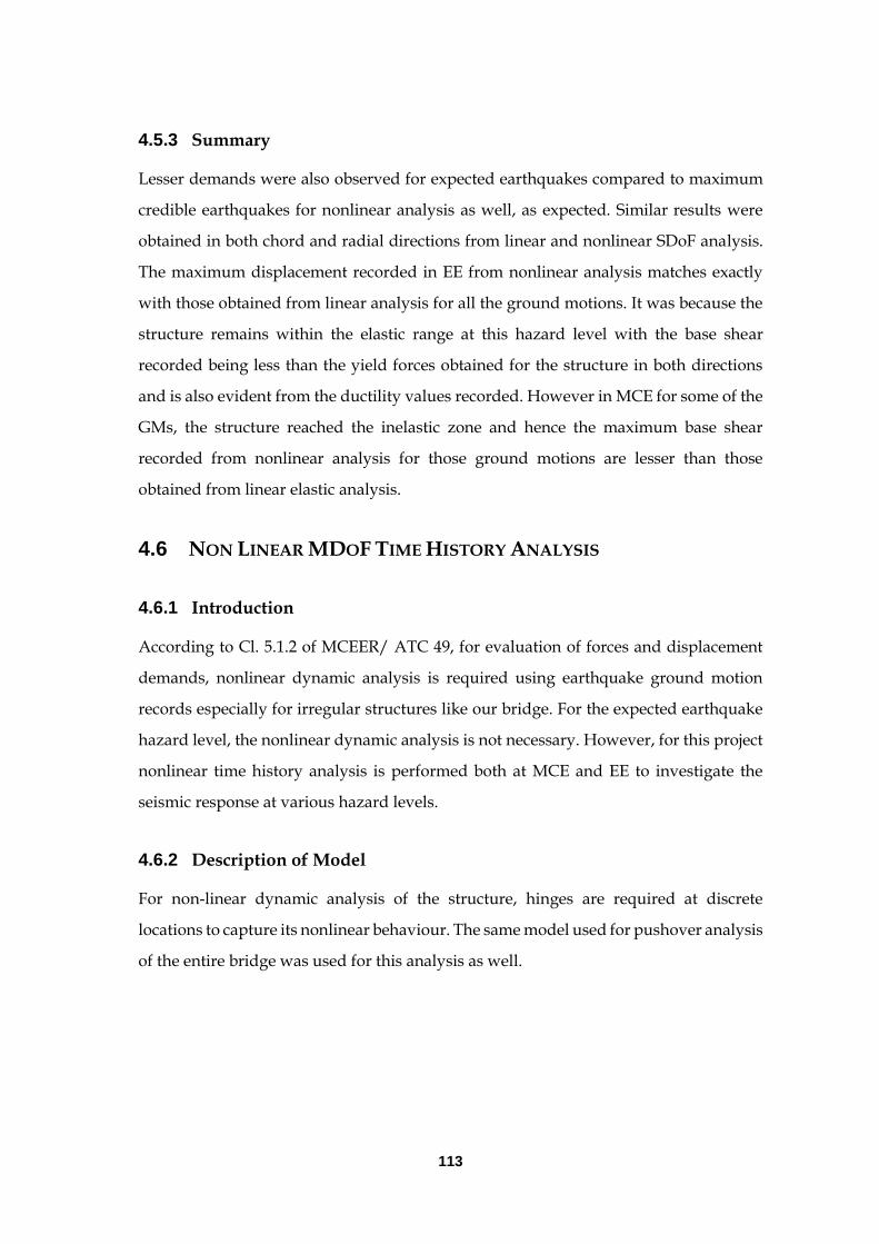
113

4.5.3 Summary

Lesser demands were also observed for expected earthquakes compared to maximum

credible earthquakes for nonlinear analysis as well, as expected. Similar results were

obtained in both chord and radial directions from linear and nonlinear SDoF analysis.

The maximum displacement recorded in EE from nonlinear analysis matches exactly

with those obtained from linear analysis for all the ground motions. It was because the

structure remains within the elastic range at this hazard level with the base shear

recorded being less than the yield forces obtained for the structure in both directions

and is also evident from the ductility values recorded. However in MCE for some of the

GMs, the structure reached the inelastic zone and hence the maximum base shear

recorded from nonlinear analysis for those ground motions are lesser than those

obtained from linear elastic analysis.

4.6 NON LINEAR MDOF TIME HISTORY ANALYSIS

4.6.1 Introduction

According to Cl. 5.1.2 of MCEER/ ATC 49, for evaluation of forces and displacement

demands, nonlinear dynamic analysis is required using earthquake ground motion

records especially for irregular structures like our bridge. For the expected earthquake

hazard level, the nonlinear dynamic analysis is not necessary. However, for this project

nonlinear time history analysis is performed both at MCE and EE to investigate the

seismic response at various hazard levels.

4.6.2 Description of Model

For non-linear dynamic analysis of the structure, hinges are required at discrete

locations to capture its nonlinear behaviour. The same model used for pushover analysis

of the entire bridge was used for this analysis as well.

114


The load cases are defined for each GM corresponding to Time History Analysis.

Analysis type is nonlinear and solution type adopted is Direct Integration. Newmark

Beta method was used with values of and equal to 0.5 and 0.25, respectively, which

represent constant linear acceleration approximation of GM.

Figure 4.3 Definition of a time history function in SAP 2000 program

115

Figure 4.4 Typical Time History Load Case defined in SAP 2000

Figure 4.5 Type of direct integration procedure followed in SAP 2000

The Raileigh damping was used for this purpose with both the first and second periods

subjected to 5% damping as shown in Figure 4.6. The mass source used for time history

analysis was similar to the modal analysis as shown in Figure 4.7.

116

Figure 4.6 Mass and stiffness coefficients for damping

Figure 4.7 Definition of mass source for time history analysis

The nomenclature for a load case for EE and MCE is shown in the Table 4.11 below

Table 4.11 Nomenclature used for defining the GMs

Load type Load name Function Scale factor

Accel U1 IV_FN_EE g X SF = 180.48 (in)

Accel U2 IV_FP_EE g X SF = 180.48 (in)

Accel U1 LP_FN_MCE 32.2 (feet)

Accel U2 LP_FP_MCE 32.2 (feet)

117

Where, LP_FN_MCE stands for Loma Prieta Fault Normal Maximum Considered

Earthquake and LP_FP_MCE stands for Loma Prieta Fault Parallel Maximum

Considered Earthquake. Similarly load cases are defined for all the ground motions for

EE and MCE.

Figure 4.8 Time history load cases defined in SAP 2000


The response of the structure in terms of joint displacement, base shear, plastic hinge

rotation and hysteretic loops are shown in Figure 4.9 to Figure 4.12 for the North Ridge

Earthquake scaled to MCE hazard level.

Figure 4.9 Maximum displacement response recorded for pier 4 during North Ridge GM

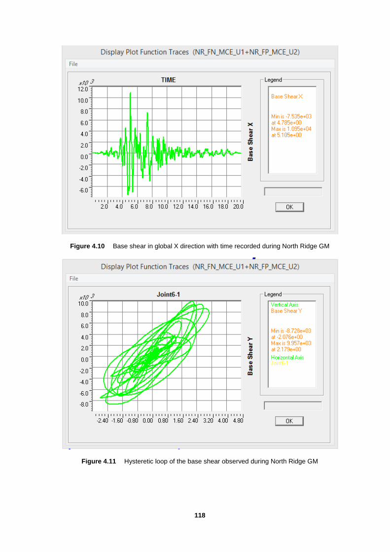
118

Figure 4.10 Base shear in global X direction with time recorded during North Ridge GM

Figure 4.11 Hysteretic loop of the base shear observed during North Ridge GM

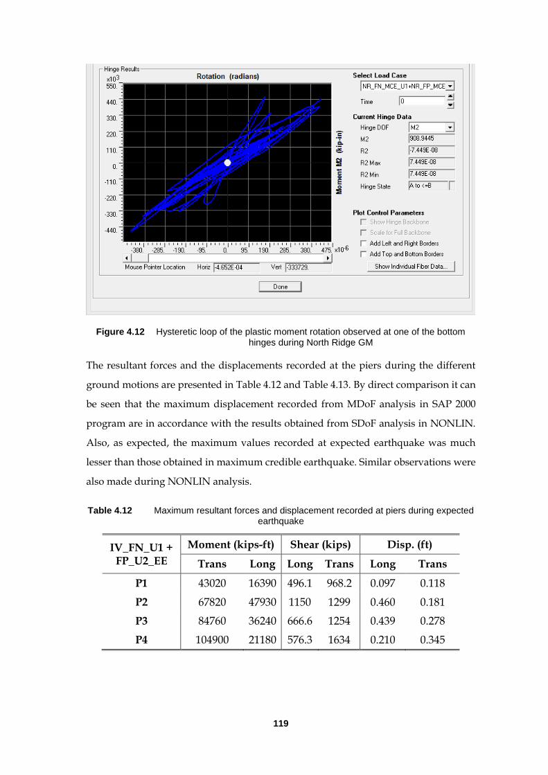
119

Figure 4.12 Hysteretic loop of the plastic moment rotation observed at one of the bottom hinges during North Ridge GM

The resultant forces and the displacements recorded at the piers during the different

ground motions are presented in Table 4.12 and Table 4.13. By direct comparison it can

be seen that the maximum displacement recorded from MDoF analysis in SAP 2000

program are in accordance with the results obtained from SDoF analysis in NONLIN.

Also, as expected, the maximum values recorded at expected earthquake was much

lesser than those obtained in maximum credible earthquake. Similar observations were

also made during NONLIN analysis.

Table 4.12 Maximum resultant forces and displacement recorded at piers during expected earthquake

IV_FN_U1 + FP_U2_EE

Moment (kips-ft) Shear (kips) Disp. (ft)


P1 43020 16390 496.1 968.2 0.097 0.118

P2 67820 47930 1150 1299 0.460 0.181

P3 84760 36240 666.6 1254 0.439 0.278

P4 104900 21180 576.3 1634 0.210 0.345

120

IV_FN_U2 + FP_U1_EE



P1 45280 11510 356.5 880.3 0.068 0.111

P2 56470 35150 858.2 999.3 0.259 0.134

P3 60950 24790 526.2 839.4 0.260 0.169

P4 71260 28210 617.3 1178 0.297 0.214

KJ_FN_U1 + FP_U2_EE



P1 86000 16400 440.1 1858 0.100 0.234

P2 65790 32000 598.8 1288 0.242 0.184

P3 68950 19920 394.6 1019 0.223 0.202

P4 86240 26730 538.3 1315 0.331 0.271

KJ_FN_U2 + FP_U1_EE



P1 65690 27380 722.5 1318 0.175 0.169

P2 101300 35830 619.9 1959 0.435 0.280

P3 104700 23790 444.8 1584 0.391 0.363

P4 93970 17300 435.1 1437 0.207 0.369

NR_FN_U1 + FP_U2_EE



P1 43160 27670 754.1 946.6 0.168 0.117

P2 45280 34330 681.7 894.4 0.261 0.128

P3 54110 22570 573 961.7 0.251 0.166

P4 59430 21780 509.5 952 0.220 0.168

121

NR_FN_U2 + FP_U1_EE



P1 52210 23940 646.2 1088 0.148 0.136

P2 49770 31980 607.8 923.6 0.250 0.126

P3 63100 22690 580.2 880.7 0.245 0.174

P4 83650 16400 475.2 1455 0.173 0.269

Maximum Moment (kips-ft) Shear (kips) Disp. (ft)


P1 86000 27670 754.1 1858 0.175 0.234

P2 101300 47930 1150 1959 0.460 0.280

P3 104700 36240 666.6 1584 0.439 0.363

P4 104900 28210 617.3 1634 0.331 0.369

Table 4.13 Maximum resultant forces and displacement recorded at piers during maximum credible earthquake

LP_FN_U1 + FP_U2_MCE



P1 102800 53740 1728 2260 0.451 0.338

P2 111000 44810 1413 2283 0.432 0.401

P3 110800 27280 1759 1728 0.436 0.466

P4 114700 31890 1559 1518 0.541 0.470

LP_FN_U2 + FP_U1_MCE



P1 122300 50910 1526 2834 0.484 0.463

P2 123100 31470 1224 2534 0.298 0.410

P3 99800 22720 2064 1361 0.312 0.411

P4 112200 30270 1824 1769 0.484 0.497

122

CM_FN_U1 + FP_U2_MCE



P1 138000 36590 1076 3302 0.543 0.492

P2 140600 56600 1340 3275 0.853 0.596

P3 128900 51320 1191 2122 0.915 0.654

P4 133400 43820 1147 1932 1.305 0.701

CM_FN_U2 + FP_U1_MCE



P1 141500 36090 892.8 3403 0.699 0.647

P2 145800 50600 1096 3003 0.720 0.801

P3 140700 35690 901.1 2325 0.633 1.106

P4 147300 34900 936.3 2462 0.988 1.124

NR_FN_U1 + FP_U2_MCE



P1 92380 42310 1284 1915 0.416 0.291

P2 95810 43890 1003 2066 0.614 0.356

P3 82020 34610 1123 1512 0.583 0.32

P4 99880 43620 980.8 1664 0.504 0.380

NR_FN_U2 + FP_U1_MCE



P1 123500 34280 1068 2577 0.467 0.387

P2 120700 39150 1075 2495 0.452 0.396

P3 133200 27660 959.2 2094 0.439 0.396

P4 144300 21350 870.8 2127 0.533 0.460

123

Maximum Moment (kips-ft) Shear (kips) Disp. (ft)


P1 141500 53740 1728 3403 0.699 0.647

P2 145800 56600 1413 3275 0.853 0.801

P3 140700 51320 2064 2325 0.915 1.106

P4 147300 43820 1824 2462 1.305 1.124


Lesser demands were also observed for expected earthquakes compared to maximum

credible earthquakes for both linear and nonlinear analysis in SAP 2000 and NONLIN

program, as expected. Similar results were obtained in both chord and radial directions

from linear and nonlinear SDoF analysis. The structure was observed to remain within

the elastic range at EE hazard level with the base shear recorded being less than the

yield forces obtained for the structure in both directions. However in MCE for some of

the GMs, the structure reached the inelastic zone. By direct comparison, it can be

observed that the maximum displacement recorded from MDoF analysis in SAP 2000

program was higher compared to SDoF analysis in NONLIN.

-o-o-o-

124

CHAPTER 5 5. CAPACITY SPECTRUM AND FLOWCHARTS

CAPACITY SPECTRUM ANALYSIS AND FLOWCHARTS


Capacity Spectral method is one of the latest analysis procedures for seismic evaluation

of a structure. In This procedure the capacity obtained from pushover analysis are

balanced with the seismic demand represented by the response spectrum at that

location. The primary objective of capacity spectrum analysis is to predict the ability of

the structure to resist a seismic event. The capacity of the structure was obtained from

the nonlinear static pushover analysis. The base shear-pier top displacement obtained

from the pushover analysis was converted into equivalent spectral acceleration and

displacement on which the response spectra curves at MCE and EE were superimposed.

Calculations were carried out until the ductility of the capacity and demand curve

matches each other. The structure will be safe during the earthquake at required

performance level, if it is designed for the ductility thus obtained from this analysis.

The flow chart prescribed in MCEER/ATC 49 report as applicable to our bridge is

presented in this Chapter.

5.2 CAPACITY SPECTRUM ANALYSIS

Capacity spectrum method is essentially a nonlinear static analysis approach which

compares the force-displacement curve of the structure with the response spectra of the

site at various hazard levels. This method applies only to structures that essentially

behave as a single degree of freedom system.

sharathchandra

Highlight

sharathchandra

Highlight

sharathchandra

Highlight

125


Assumptions

1. To calculate the Seismic Capacity Coefficient Cc for the piers, the tributary

weight of the superstructure supported by the individual piers is the only

seismic load considered.

2. The abutments take very less seismic load, hence their contribution to seismic

resistance is considered negligible.

3. The Δy value is taken as 1.3 times the Seismic Capacity Coefficient Cc found

using the lateral strength and the weight of the structure.

Calculations

To check the applicability of the equations given in Commentary section 5.4.1.1(C4.4-1)

MCEER-ATC 49 , the natural time period of the structure is compared with the Ts of

both Expected and Maximum Considered Earthquake.

With a Tn of 1.54 secs in longitudinal direction and 0.88 secs in the transverse direction

which are greater than their corresponding Ts values of 1.42 secs and 0.77secs, the

structure was found to be in velocity sensitive region for both MCE and EE.

As per MCEER-ATC –C5.4.1 , bridges that have elastomeric or sliding bearings at each

pier shall be designed as an isolated structure using the provisions of Article 5.4.1.2 and

Article 15.

The BL factor was obtained from table 5.4.1-1, where BL values are for configurations

where the columns are primary resisting elements.

From MCEER-ATC 49-5.4.1.-1,

2

11

2

2v

C

L y

nc

gF SC

B

VC

W

The values for calculating the displacements were obtained from the Push over analysis

and are tabulated below for reference.

126

Table 5.1 Comparison of results from various analysis procedure

From Pushover

𝑽𝒏

(kips)

θp

(rad)

Trans Long Trans Long

50ft 2300 920 0.0112 0.0427

70ft 2250 720 0.0143 0.0548

Entire bridge 26000 4300 0.057 2.01

Sample calculation:

EE (Operational and Life safety)- Transverse direction

Cc *∆𝑦 = 2.02*4*1.3 = 21.84

(𝐹𝑣.𝑆1

2𝜋𝐵𝐿)

2. 𝑔 = (

1.685∗.0.115

2𝜋∗1)

2∗ 386.4 = 0.367 < 21.84 𝑆𝑎𝑓𝑒

The bridge is expected to meet the performance requirement for the expected

earthquake.

MCE – Life Safety –Longitudinal direction

∆𝑦 =1

Cc*(

𝐹𝑣.𝑆1

2𝜋𝐵𝐿)

2. 𝑔 =

1

0.334*(

1.3∗0.527

2𝜋∗1.6)

2∗ 386.4 = 5.372

θp*H = 0.035*50 = 1.75 < 5.372 Not safe

From MCEER-ATC 49 (Commentary),from equation C4.4-6,

We take ∆𝑦 = 1.75,

Required Seismic Coefficient Cc =1

∆𝑦*(

𝐹𝑣.𝑆1

2𝜋𝐵𝐿)

2. 𝑔 =

1

1.75*(

1.3∗0.527

2𝜋∗1.6)

2. 386.4 = 1.023

The required lateral strength is 𝑉𝑛 = Cc * W =1.023* 12871.2 = 13174.017 kips

MCE – Operational –Longitudinal direction

P – Δ check :

0.25 CcH = 0.25* 0.334* 50 = 4.175 < 13.728 (Not safe)

From MCEER-ATC 49 (Commentary),from equation C4.4-7,

We take ∆𝑦 = 13.728,

Required Seismic Coefficient Cc = 4*𝚫

H =1.098

EE (Operational and Life safety)

127

.Table 5.2 Summary of Cc values at EE

Limiting value = 0.367 Cc *∆𝒚

Longitudinal (L) 1.389 (safe)

Transverse (T) 21.84 (safe)

Table 5.3 Summary of operational performance level at MCE

Dir. ∆𝒚 θp*H 0.25 CcH Modified Cc

Modified Vn θp*H P–Δ

L 13.72 1.75 4.175 2.62 1.098 33722.54

T 2.27 1.75 25.25 2.62 - 33722.54

Table 5.4 Summary of life safety performance level at MCE

Dir ∆𝒚 θp*H 0.25 CcH Modified Cc Modified Vn

L 5.372 1.75 4.175 2.62 13174.017

T 0.888 1.75 25.25 - -

The bridge is expected to be safe for Expected earthquake. For MCE, the bridge was

found to be safe only for Life safety performance along the transverse direction and

unsafe for the rest of the cases. The required lateral strength for the unsafe cases was

calculated to be 33722.54 kips in transverse direction and 13174.017 kips in longitudinal

direction. As for the rest of the cases, the bridge seems to have enough capacity to

withstand the demand displacement for both Expected and Maximum Considered

earthquakes for Operational and Life safety performances as can be seen from the

calculations done based on MCEER-ATC(49) -5.4.1-1(C4.4-1).

5.3 FLOWCHARTS

The following design charts illustrate the process that should be followed for design

and analysis of a bridge project such as the one shown in this report. While the design

charts illustrate several different options for analysis, not all being necessary, please

note that LP has explored all of these options. The results from such analyses are shown

in further depth within the earlier chapters of this report.

131

Figure 5.1 Flowchart as applicable to our bridge

132


It was observed from the results that the entire bridge wasn’t safe for Expected

earthquake in the longitudinal direction. The same was observed in the case of 70 feet

piers too. As for the rest of the cases, the bridge seems to have enough capacity to

withstand the demand displacement for both Expected and Maximum Considered

earthquakes for Operational and Life safety performances.

-o-o-o-

133

CHAPTER 6 6. FINAL CONCLUSIONS

FINAL CONCLUSIONS


The bridge example 5 of Federal High Way Authority (FHWA) was analyzed at a

different site at Tacoma with certain modifications in the geometry of the bridge as

described in Chapter 1. However the material properties of the bridge along with the

soil conditions were taken directly from the original example. Various analysis as

mentioned in MCEER /ATC 49 report were performed on the bridge as a part of the

project including simple SDOF analysis to more sophisticated nonlinear MDOF time

history analysis. The resultant demand on the structure in terms of maximum bending

moment, shear force and displacement obtained from the various analysis procedure

are compared in this Chapter. The performance of the bridge at MCE and EE was

evaluated by comparing the demand with the capacity of the columns. The safety of the

bridge at MCE and EE and further recommendations are also stated.

6.2 COMPARISON FROM VARIOUS ANALYSIS PROCEDURE

The comparison of the uniform load method, multimode response spectrum analysis,

linear and nonlinear time history analysis were carried out with respect to the maximum

shear force, bending moment and displacement recorded at the piers and presented in

table. It must be noted that 100-40 combination was carried out in both uniform load

method and multimode method so that the results can be compared.

134

Table 6.1 Comparison of results from various analysis procedure

Maximum Values

Expected earthquake Maximum Credible earthquake

Shear (kips)

Moment (kips-feet)

Displacement (feet)

Shear (kips)

Moment (kips-feet)

Displacement (feet)

Long Trans Trans Long Long Trans Long Trans Trans Long Long Trans

Uniform Load method

793 624 45482 45988 0.24 0.12 2217 2802 161485 162499 0.85 0.44

Multimode analysis

761 657 52668 35293 0.18 0.15 2326 2693 186280 124783 0.64 0.51

Elastic Time History

Analysis 672 2058 127500 42417 0.34 0.35 2850 7810 495833 152500 1.33 1.16

Inelastic Time History analysis

1150 1959 104900 47930 0.46 0.37 2064 3403 147300 116600 1.31 1.12

135

The maximum shear force at MCE as obtained from uniform load method, multimode

analysis, linear and nonlinear time history analysis are 2217 kips, 2326 kips, 2850 kips

and 2064 kips, respectively considering all the cases. The maximum moment from the

analysis are 162499 kip-ft, 124783 kip-ft, 152500 kip-ft and 116600 kip-ft, respectively.

These results are for longitudinal direction of the piers. The maximum displacement

from these four analysis procedures at MCE in the longitudinal direction are 0.85 ft, 064

ft, 1.33 ft and 1.31 ft, respectively. The corresponding transverse displacements are 0.44

ft, 0.51 ft., 1.16 ft. and 1.12 ft. From direct comparison it can be concluded that the results

obtained from various procedures are in close agreement with each other, especially as

far as the shear force and displacements are concerned. However, bending moment in

some of the cases are different and the possible reason is the irregular curved geometry

of the bridge.

6.3 PERFORMANCE OF STRUCTURE

As it was observed from the response spectra curves at MCE and EE for our site, there

is a large difference in the hazard level, with the maximum spectral acceleration at short

periods is almost thrice for MCE compared to EE. So it is likely, that the designed bridge

should perform better during expected earthquake, but possibly cannot survive the

maximum credible earthquake hazard level.

The maximum demands obtained in the earlier chapters for multimode analysis,

uniform load method, elastic and inelastic time history analysis were compared with

the capacity of the piers from pushover analysis and the performance of the bridge is

investigated both at MCE and EE for operational and life safety performance levels. The

maximum demands obtained for the linear elastic analysis cases was to be divided by

the response reduction factor (R) as per MCEER/ATC 49 report based on the following

equation.

1 ( 1)1.25

B B

S

TR R R

T

where, RB can be obtained from Table 4.7.1 of the MCEER report and T is the period of

the structure in the respective direction. Detailed calculations were carried out for all

the four analysis cases and the safety of the bridge at various performance levels are

summarized in Table 6.2 and Table 6.3.

136

Table 6.2 Calculation of R factor at EE and MCE

Steps

EE MCE


Life Safety Operational Life Safety Operational Life Safety Operational Life Safety Operational

Sd1 0.193 0.193 0.193 0.193 0.685 0.685 0.685 0.685

Sds 0.396 0.396 0.396 0.396 1.298 1.298 1.298 1.298

Ts 0.487 0.487 0.487 0.487 0.528 0.528 0.528 0.528

1.25Ts 0.609 0.609 0.609 0.609 0.660 0.660 0.660 0.660

T 1.54 1.54 0.88 0.88 1.54 1.54 0.88 0.88

T/(1.25Ts) 2.528 2.528 1.444 1.444 2.335 2.335 1.334 1.334

Rb 1.3 0.9 1.3 0.9 4 1.5 4 1.5

(Rb-1) 0.3 -0.1 0.3 -0.1 3 0.5 3 0.5

(Rb-1)*(T/1.25Ts) 0.76 -0.25 0.43 -0.14 7.00 1.17 4.00 0.67

R 1.76 0.75 1.43 0.86 8.00 2.17 5.00 1.67

Final R 1.300 0.750 1.300 0.860 4.000 1.500 4.000 1.500

137

Table 6.3 Performance evaluation of the structure

Analysis

Maximum Moments

EE MCE


Life Safety Operational Life Safety Operational Life Safety Operational Life Safety Operational

ULM 45988 45988 45482 45482 162499 162499 161485 161485

ULM/R 35375 61317 34986 52886 40625 108332 40371 107656

ULM 35293 35293 52668 52668 124783 124783 186280 186280

MM/R 27148 47057 40514 61242 31196 83189 46570 124187

Elastic THA 42417 42417 127500 127500 152500 152500 495833 495833

Elastic THA/R 32628 56556 98077 148256 38125 101667 123958 330556

Inelastic THA 47930 47930 104900 104900 56600 56600 147300 147300

Capacity of the pier obtained from pushover analysis

Moment Capacity

35000 35000 100000 100000 35000 35000 100000 100000

Final Conclusion on the performance of the bridge

ULM Safe Unsafe Safe Safe Unsafe Unsafe Safe Unsafe

MM Safe Safe Safe Safe Unsafe Unsafe Unsafe Unsafe

Elastic THA Safe Unsafe Safe Safe Safe Unsafe Safe Unsafe

Inelastic THA Unsafe Unsafe Unsafe Unsafe Unsafe Unsafe Unsafe Unsafe

138

Therefore it can be concluded that performance of bridge remains operational in case of

EE but leads to possible failure in MCE.

6.4 SCOPE OF FUTURE WORK

The scope for future work is presented in this section

1. A more sophisticated model of the bridge (3D) with better computing capability

can improve the results obtained from MDOF nonlinear time history analysis

2. P-delta effects can be included to consider geometrical nonlinearity.

3. Time history analysis was carried out only according to seismic hazard as per

ATC MCEER 49 document. In future time history analysis can also be performed

with hazard level defined in AASHTO document.

6.5 RECOMMENDATIONS FOR IMPROVEMENT OF PERFORMANCE

The performance of the bridge was unsatisfactory at MCE. Therefore, recommendations

have been presented in this section to ensure collapse prevention of the existing bridge

at MCE.

1. The bearings used in the present model were simple bridge bearings, which

were good enough for small displacement demands at EE but cannot

accommodate the high displacement demand at MCE. Therefore, seismic

isolation bearings can be used to accommodate the excess displacement

demands during high seismic event. Sliding friction pendulum bearings can be

a good alternative to those used in the present model to ensure better

performance at MCE.

2. Use of dampers along with the isolators can also improve the performance of the

bridge at high earthquakes.

3. All the piers can be converted to sliding piers to accommodate the high

displacement demands expected at MCE.

-o-o-o-

139

APPENDIX A –C1

VALIDATION OF MODEL

The model of the bridge produced in the SAP 2000 program and some of the

assumptions made during modelling are validated using simpler examples. The

description of calibration examples used to verify elastic analysis modelling options of

SAP 2000 are discussed in this section. The model bridge is subjected to uniform lateral

load, hence an elastic analysis of a portal frame subjected to lateral load is carried out in

SAP 2000 program. Moment diagrams and shear forces obtained from the program are

compared with the known analytical results. In addition, multi span continuous beam

with spring supports are analyzed to validate the spring models which are used in SAP

2000 model to account for the foundation stiffness’s. In the present project, the

superstructure is a composite element with concrete deck and steel girders, however,

for simplicity equivalent transformed concrete section was used to model the

superstructure behaviour. For validation of the use of equivalent concrete section in the

bridge model, a simply supported steel bridge is transformed into an equivalent

concrete section and their deflections are compared.

Validation of Elastic Analysis in SAP 2000

A single story single bay frame as shown in Figure A1 was modelled in SAP 2000

[CSI, 2009] program to calibrate/validate the static analysis procedure used in this

project. The bending moment and shear force diagrams obtained from the SAP 2000

program was compared with the results obtained analytically. For simplicity, a statically

determinate portal frame (Figure A1) analyzed in the text book “Fundamentals of

Structural Analysis” (Example 5.5) was used for this purpose. The shear force and the

bending moment diagram obtained in SAP 2000 program are presented in Figures A2

and A3, respectively.

140

Figure A1 Simple portal frame

Figure A2 Shear force diagram obtained from SAP 2000

Figure A3 Bending Moment Diagram obtained from SAP 2000

Analytical results obtained from Text Book

The free body diagram of the frame members and the bending moment and shear force

diagram as presented in the text book is shown in Figure A4

141

Figure A4 Analytical results obtained from text book [Chakraborty et al. 2009, Example 5.5]

Thus it can be seen from the Figures, that the bending moment and shear force diagrams

obtained from SAP 2000 program and analytically from the text book matches with each

other. Hence, the static/elastic analysis procedure of SAP 2000 is validated.

Validation of spring stiffness in SAP 2000

A spring of K = 10 kN/m was modelled in SAP 2000 program and a load of 5kN (P) was

applied at the node. So, deflection, can be obtained analytically as,

P

K

From the above equation, the deflection of the node comes out to be 0.5 m, which was

also obtained in the SAP 2000 program as shown in Figure A4 and hence in agreement

with the analytical result. Therefore, spring supports can be used in the bridge model to

account for the foundation stiffness. A simple multi-span beam with spring at one

support was also analyzed in SAP 2000 program to further validate the spring model.

142

Figure A5 Spring model analyzed in SAP 2000

Multi span beam with spring at one support

A 12m two-span beam (Figure A5), with a spring of K = 1 kN/m at the middle and a

load of 20kN quarter point was analyzed in SAP 2000 program. The cross section of the

beam was considered as 5000 mm square and material was assumed to be concrete with

elastic modulus 25000 MPa. The deflection, and the reaction, R of the spring obtained

in SAP 2000 program was compared with the values obtained analytically.

Figure A6 Multi span continuous beam with spring support analyzed in SAP 2000

As can be seen from Example 10.6 of text book “Fundamentals of Structural Analysis”,

R and can be obtained according to the following equations.

3

3

11 768

48 1

PL EIR

L EI K

3 311

48 768

RL PL R

EI EI K

From these equations R comes out to be 147.12 N and deflection of spring comes out to

be 0.147 mm which is in good agreement with the values obtained in SAP 2000 program

as can be seen in Figures A7 and A8.

Figure A7 Reaction at supports of the multi span continuous beam obtained in SAP 2000

143

Figure A8 Deflection of the continuous beam at spring support obtained from SAP 2000

Hence it can be concluded, that spring model can be used in SAP 2000 program to take

into account the foundation stiffness.

Validation of equivalent concrete rectangular section in SAP 2000

A simply supported beam with 2 – 6 m spans (Figure A9) is analyzed in SAP 2000, first

considering the cross section to be steel I-section and then transforming the section as

shown in Figures A13 to A15 into an equivalent concrete section using modular ratio of

8. However, while transforming the steel section into concrete, the moment of inertia of

the concrete section was made equal to the transformed steel section, but the cross-

sectional area was not equal. Therefore, area modifier property in SAP 2000 was used

for proper transformation of the cross-section. The area modifier factor was calculated

as 0.416 as the ratio of the cross- sectional area of the actual transformed steel section to

that of the equivalent concrete section. The deflection under the point loads are

calculated and it was observed to be similar for both the cases.

Figure A9 Beam used for validation of transformed section in SAP 2000

144

Figure A10 Cross-section details of the actual steel section

Figure A11 Sectional properties of the actual steel cross-section

Figure A12 Deflection of the original steel beam

145

Figure A13 Cross-sectional details of the transformed steel section

Figure A14 Sectional properties of the transformed steel cross-section

146

Figure A15 Sectional properties of the transformed concrete cross-section

Figure A16 Deflection of the transformed equivalent concrete beam

As it can be seen from Figures A12 and A16, the maximum deflection of the beam is

same for both the original steel section and the transformed concrete section. Hence, the

equivalent transformed section concept is validated and therefore, used in the present

project to simulate the superstructure behaviour in SAP 2000.

-o-o-o-

147

APPENDIX A –C2

VALIDATION OF MODEL

The modal analysis procedure of the SAP 2000 program is validated using simpler

example. The response spectra parameters for our site was obtained from the ATC 49

report and matched with the design spectra obtained from the USGS website. A simple

lumped mass model with known spring stiffness was developed in NONLIN program

and its response obtained is matched with the analytical solution for calibration. The

response spectra obtained from PEER strong motion database was also matched with

the one obtained analytically.

Calibration of Eigen Value Analysis in SAP 2000

A three story single bay frame as shown in Figure A18 was modelled in SAP 2000

[CSI, 2009] program to calibrate/validate the modal analysis procedure used in this

project. The frame used in the validation of modal analysis was taken from the text book

“Dynamics of Structures: Theory and Applications to Earthquake Engineering”

[Chopra, 2005] and the sections and geometric dimensions were chosen arbitrarily to

get numerical values for comparison with SAP 2000 results. The natural frequencies and

the corresponding mode shapes obtained in SAP 2000 program was compared with the

analytical results and presented in this section.

Height (h) 12 feet

Weight 10 kips

Mass (m) 25.91 lbs-sec2/inch

Elastic Modulus (E) 29000 ksi

Moment of Inertia (I) 184 in4 [W 8 X 48 sections]

148

Figure A18 Mass Source considering only the weight of the superstructure

Analytical Solution

Stiffness from 2

columns

348EI h

Equation of motion 3 3

2 2

3 3

2 0 0 0

0 0 2 0

0 0 0 2

m u k k u

m u k k k u

m u k k u

Eigen Value

Problem 2 0M K

Solution

1

2

3

21.06 rad/s

57.54 rad/s

78.60 rad/s

2Period =

1 1

2 2

3 3

0.30 s 3.34 Hz

0.11 s 9.15 Hz

0.08 s 12.5 Hz

T f

T f

T f

149

Mode 1 Mode 2 Mode 3

Figure A19 Mode shapes obtained analytically

SAP 2000 Model

The three story frame presented in Figure A18 was modeled in SAP 2000 program and

the modal analysis was done along XZ plane to ensure planer behaviour. The column

sections were selected as W 8X48 with E = 29000 ksi and considered fixed at their base.

The beams were considered to be rigid elements and hence the E of beam was increased

to 2.9 X E10 ksi. The masses were assumed to be lumped at the center nodes of the beams

at each floor level. The comparison of the results obtained analytically and in SAP 2000

program is presented in Table A1. The mode shapes obtained are shown in Figure A20.

150

Mode-1 Mode 2 Mode 3

Figure A20 Mode Shapes obtained from SAP 2000

Table A1 Comparison of natural frequencies obtained from SAP with analytical results

Mode Analytical Solution SAP 2000

1 Freq. (Hz) 3.34 3.28

Period (s) 0.30 0.31

2 Freq. (Hz) 9.15 9.17

Period (s) 0.11 0.11

3 Freq. (Hz) 12.5 12.8

Period (s) 0.08 0.08

So it can be seen from Table A1 and Figures A2 and A3, the natural frequencies and the

corresponding mode shapes obtained from SAP 2000 program are in close agreement

with the analytical solution, which validates modal analysis procedure of the software.

Validation of USGS Ground Motion Information and Response Spectra

The response spectra was developed based on the procedure prescribed in MCEER

ATC 49, Section 3.4.1. For maximum credible earthquake, the values of spectral

acceleration at short period, SMS and the spectral acceleration at 1 s period, SM1, were

obtained according to the following equations,

MS a SS F S

1 1M vS F S

151

where, the values of SS and S1 were obtained from Fig. 3.4.1-2(a) and Fig. 3.4.1-2 (b)

[USGS Hazard Maps presented in ATC 49], and the values Fa and Fv were obtained from

Tables 3.4.2.3-1 and 3.4.2.3-2, respectively, of MCEER ATC 49 for our location [Latitude

= 47.25N and Longitude = 122.44W] and site class C [very dense soil and soft rock]. The

Table A2 presented the calculation of the values from ATC 49 and compared with the

values obtained from USGS website for Maximum Credible Earthquake (MCE). It can

be seen that the % variation from the ATC 49 document is even less than 1% and

therefore, the response spectra obtained from the USGS website can be used as the

design spectra for our site. The parameters for Expected Earthquake (EE) were also

obtained using the same procedure and hence, the calculations are not shown

separately.

Table A2 Comparison of response spectra parameters for MCE

Source Ss (g) S1 (g) Fa Fv SMS (g) SM1 (g)

ATC 49 1.30 0.53 1.0 1.3 1.30 0.689

USGS 1.298 0.527 1.0 1.3 1.298 0.685

Variation (%) 0.4 1.0 0 0 0.4 0.6

Calibration of SDoF Model in NONLIN Program

The example used to validate the calculations in NONLIN were taken from Example 6.2

[Chopra, 2008]. The problem is a SDOF system and important values are as follows:

𝑊𝑒𝑖𝑔ℎ𝑡 = 𝑊 = 5200 𝑙𝑏

𝑆𝑡𝑖𝑓𝑓𝑛𝑒𝑠𝑠 = 𝐾 = .211𝑘𝑖𝑝

𝑖𝑛

𝑀𝑎𝑠𝑠 = 𝑚 =𝑊

𝑔=

5.2

386= 0.01347 𝑘𝑖𝑝 ∗

𝑠𝑒𝑐2

𝑖𝑛

𝐷𝑎𝑚𝑝𝑖𝑛𝑔 = 𝜉 = 2%

Natural frequency and period: 𝜔𝑛 = √𝑘

𝑚= √

0.211

0.01347= 3.958 𝑟𝑎𝑑/𝑠𝑒𝑐

𝑇𝑛 = 1.59

From Response Spectrum Shown Below,

152

Figure A21 Response Spectrum of the GM considered [Chopra 2008, Figure 6.8.3]

For 𝜉 = 2%, 𝑇𝑛 = 1.59, 𝐷 = 5.0 𝑖𝑛𝑐ℎ𝑒𝑠, 𝑎𝑛𝑑 𝐴 = 0.2𝑔,

𝑀𝑎𝑥𝑖𝑚𝑢𝑚 𝐷𝑖𝑠𝑝𝑙𝑎𝑐𝑒𝑚𝑒𝑛𝑡 = 𝑢0 = 𝐷 = 5.0 𝑖𝑛𝑐ℎ𝑒𝑠

In order to run this analysis in NONLIN, the inputs were a lumped mass of 5200 lbs, 2%

damping, and 211 lb/in, run in linear, simple bilinear analysis. A ground motion at

Imperial Valley was implemented, to match the El Centro ground motion from the

above example, and a maximum of 0.2g was applied on the ground acceleration as

described in the Example.

The results of the analysis are 5.223 inches displacement. There is only 4.36% difference

between the calculated value in the textbook and NONLIN and is therefore acceptable.

These values can be seen in the following Figure. As an additional check, it is noted that

the period calculated in NONLIN is 1.587, therefore matching that of the example and

hence validated.

153

Figure A22 NONLIN output of the Example Problem

Calibration of the Program used for Response Spectrum Development

The target spectrum was scaled using the Ground Motion data for various places

obtained from the PEER Ground Motion database based on the magnitude range

specified. The validity of the time history- ground motion data /graphs extracted from

PEER was ensured by checking it against the already available ground motion data of

two sites,namely, Landers and Northridge in California, with the spectrums from PEER.

In PEER, we select the ‘Unscaled’ option to get the Response Spectrum for a particular

site whose vibrations were recorded from a station,which needs to be specified too.

Shown below is the procedure followed to subtantiate the results used .

154

The Landers Earthquake

Figure A23 Landers Earthquake Time history [Villaverde, Figure 5.31]

The Time history GM spectrum(Velocity v/s Time) for the Landers Earthquake : a)Fault

Parallel b) Fault Normal

Figure A24 Spectral Acceleration values

155

Components of ground horizontal velocity corresponding to the ground acceleration

records obtained at Lucerne Valley Station during the 1992 landers, California

earthquake.

Figure A25 PEER Output File

The Peak Ground Velocity values for both Fault Normal and parallel calculated from

the graphs in the text book are:

Normal : Close to 120 cm/s

156

Parallel : Close to 35 cm/s

From PEER : Normal : 142.878 cm/s

Parallel : 36.1024 cm/s

Figure A26 Northridge earthquake time history [Villaverde, Figure 5.32]

The time history graph (Acceleration v/s Time) for the Northridge Earthquake : a)Fault

Normal b) Fault Parallel

Figure A27 Spectral Acceleration Values

Components of ground horizontal acceleration corresponding to to the ground

acceleration records obtained at Rinaldi receiving station during the 1994 Northridge,

California earthquake.

We can clearly see that the graphs obtained from PEER match the ones from the

Textbook.

157

Figure A28 PEER Output for Northridge

The Peak acceleration values for both Fault Normal and parallel calculated from the

graph in the text book are:

Normal : Close to 425 cm/s2

Parallel : Close to 800 cm/s2

From PEER : Normal : 0.8698 g = 0.8698 * 9.8 * 100 = 852 cm/s2

Parallel : 0.4236 g = 0.4236 * 9.8 * 100 = 415 cm/s2

158

Calibration of Response Spectra

Figure A29 Response Spectrum in tripartite representation of Imperial Valley Earthquake (El Centro Station) [Villaverde, Figure 6.5]

Figure A30 Response Spectrum of Imperial Valley Earthquake from PEER ground motion database (El Centro Station Array#5)

159

Table A3: SA values obtained from Textbook

Period PEER GM database Textbook

SA (g) SA (g)

0.1 0.43 0.42

0.2 0.42 0.41

0.4 0.39 0.4

0.6 0.47 0.46

0.8 0.795 0.80

0.6 0.47 0.46

The response spectrum for Imperial Valley earthquake extracted from PEER GM

database is checked with figure A12 and we obtained the same results. Hence it’s

acceptable and validated.

-o-o-o-

160

APPENDIX A-C3

VALIDATION OF MODEL

The model of the bridge produced in the SAP 2000 program and some of the

assumptions made during modelling are validated using simpler examples. The

description of calibration examples used to verify elastic analysis modelling options of

SAP 2000 are discussed in this section. The model bridge is subjected to uniform lateral

Validation of Pushover Analysis and Fiber PMM hinge in SAP 2000

A single story single bay frame as shown in Figure A1 was modelled in SAP 2000

[CSI, 2009] program to calibrate/validate the static analysis procedure.

Plastic Hinge

In order to validate the pushover analysis performed in SAP 2000, the nonlinear static

displacement capacity verification, commonly known as ‘Pushover Analysis’ is

performed on a single degree of freedom structure. The strength of the component is

taken as a function of the displacement component, which is found by performing a

lateral load displacement analysis accounting for the nonlinear behavior of the

structure.

Here, we study a cantilever subjected to a point load of 1 KN which is increased

gradually until a target displacement of 1 feet is reached, thus determining its strength

capacity which is a function of the element’s displacement. The plastic hinge length is

assumed to be 0.1 times the length of the cantilever column.

Section used: W12 X 40.

Member length: 1 feet

161

Fig. A31 Resultant base shear Vs Monitored Displacement

The maximum shear developed during pushover by the element is 23.04 kips.

Fig. A32 Hinge Result: Plastic Moment Capacity of the pier

162

Fig. A33 Moment curvature of the section used.

From the moment curve of the section, we see the moment capacity is 276 kips-ft.

For the cantilever section considered the maximum shear capacity of the section

is 276

12 = 23 kips .

From the pushover graph we can see that , the maximum shear developed

is 23.04 kips ~ 23 kips.

The plastic moment capacity of the pier = Mp = 274 kips-ft

The corresponding plastic shear developed = 𝑀𝑃

12 =

274

12 = 22.833 kips

This shows that the base shear developed during push over almost reaches the shear

carrying capacity of the section and thus results in the development of a plastic hinge at

the base of the cantilever.

Sensitivity of Plastic Hinge Length

The plastic hinge length of the calibration example was changed from 0.1 to 0.2 and 0.3

times the length of the member to see the effect of hinge length on the lateral load

displacement capacity of the member. As it can be seen from the Figure, there is not

much difference in the ultimate lateral strength of the structure with variation of the

plastic hinge length. However, the stiffness decreases as the plastic hinge length

increases along with a slight increase in lateral strength. Therefore, the plastic hinge

163

length in the present project was calculated in accordance with the equation given in

Article 8.8.6 of MCEER/ATC 49.

Fig. A34 Effect of hinge length on force displacement relationship.

-o-o-o-

0

5

10

15

20

25

30

0 0.2 0.4 0.6 0.8 1 1.2

Lp=0.1 Lp=0.2 Lp=0.3

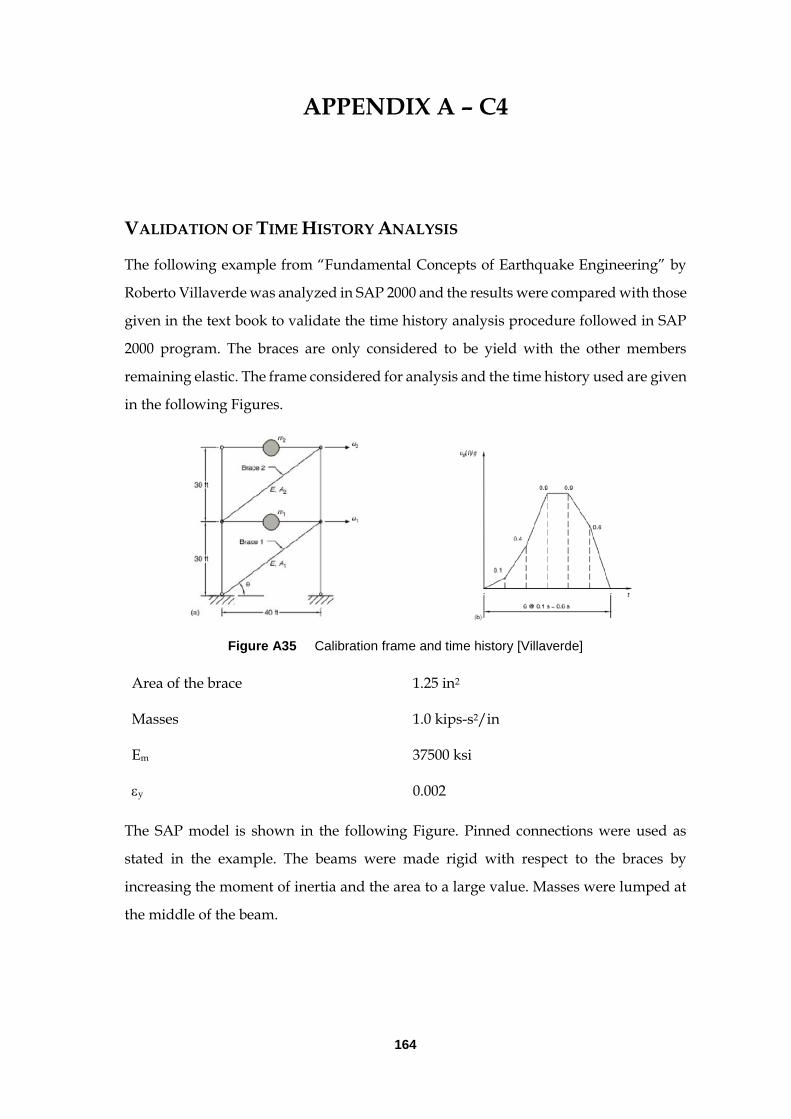
164

APPENDIX A – C4

VALIDATION OF TIME HISTORY ANALYSIS

The following example from “Fundamental Concepts of Earthquake Engineering” by

Roberto Villaverde was analyzed in SAP 2000 and the results were compared with those

given in the text book to validate the time history analysis procedure followed in SAP

2000 program. The braces are only considered to be yield with the other members

remaining elastic. The frame considered for analysis and the time history used are given

in the following Figures.

Figure A35 Calibration frame and time history [Villaverde]

Area of the brace 1.25 in2

Masses 1.0 kips-s2/in

Em 37500 ksi

y 0.002

The SAP model is shown in the following Figure. Pinned connections were used as

stated in the example. The beams were made rigid with respect to the braces by

increasing the moment of inertia and the area to a large value. Masses were lumped at

the middle of the beam.

165

Figure A36 Calibration frame and time history

The ground motion was inputted into the SAP 2000 program as shown in the Figure

A37. The nonlinear behaviour of the braces were given in form of discrete hinges using

default PMM fiber hinges as defined for the time history analysis in the present project.

The hinge definition is shown in the following Figure A38. Hinges were provided at the

middle of the braces. The nonlinear time history analysis case was then run in SAP 2000

following the same procedure as described in Chapter 5 and the results obtained are

presented in the following Table.

Figure A37 Time history defined in SAP 2000

166

Figure A38 Hinge definition in SAP 2000

Table A4 Comparison of the results obtained in SAP 2000 with textbook

Time Steps U1 (SAP) (in) U2 (Book) (in)

2 0.0684 0.0685

4 0.6048 0.6050

6 -2.5123 -2.4738

8 -6.9781 -6.6135

10 -14.4231 -13.2758

12 -22.1234 -21.4458

14 -30.1256 -29.3837

16 -38.1123 -36.3561

18 -42.1132 -41.9192

20 -45.8978 -45.7438

So the results obtained in SAP 2000 program are in accordance with those given in text

book and hence the procedure followed for non linear time history analysis is validated.

-o-o-o-

167

APPENDIX B – TEAM MANAGEMENT

Table B1 Worksheet for the Project

Weeks Amy Sandhya Sathvika Sharath Supratik

Week 2 Management plan Management plan Management plan Management plan Management plan

Week 3

Peer review of team management plan

Write up review

Peer review of team

management plan

Peer review of team

management plan

Peer review of team

management plan

Peer review of team

management plan

Week 4

Development of final team management plan

Write up for final team management plan

General description of bridge

Calculations related to stiffness values for substructure

Development of SAP2000 model of the bridge

Established the assumptions made for the analysis of the bridge

Calculations related to the various elements in the superstructure

Development of final team management plan

Calculation of stiffness values of substructure

Report for week four work

Calculation of stiffness values of superstructure

Development of SAP2000 model of the bridge

Uniform load method analysis in SAP2000

critical assessment of bridge behavior under UDL

Calibration of SAP2000

Formatting of report

168

Week 5 Report for peer team

Development of peer team bridge model in SAP2000

General bridge analysis by SAP for peer team

Modal analysis for peer review team using SAP2000

Development of peer review bridge in SAP2000

Critical assessment of the peer bridge behavior

Week 6

Maximum ground motion acceleration values

NONLIN SDOF analysis trials and final model

Time history analysis in NONLIN

Validation trials and final model in NONLIN

Response to the peer review report of the reviewer

Generation of design spectra by USGS and PEER GM Database

Generating and scaling of GM spectra for EE and MCE

Seismic design spectra of the site

Generation of design spectra by USGS and PEER GM Database

Scaling of GM

Report for review 3

Generating and scaling of GM spectra

Calibration of response spectral analysis developed by PEER

Response to the peer review team of our reviewer

Modal analysis of SAP2000 model

Review of design spectra and scaling of GMs

Development of SDOF model in NONLIN

Time history analysis in NONLIN program

Calibration of modal analysis in SAP2000

Calibration of response spectra developed from USGS

169

Week 7 Peer Review of NONLIN Analysis

Peer review of time history and response spectra

Peer review of ground motion scaling

Peer Review Report

Peer review of time history and response spectra

Peer review of ground motion scaling

Peer review of eigenvalue analysis

Week 8 Spring Break Spring Break Spring Break Spring Break Spring Break

Week 9

Elastic Analysis Multimode Dynamic Method

Multimode Validation

Hour Sheets for Appendix B

Uniform Load Method

Uniform Load Validation


Pushover Analysis


Uniform Load Method

Pushover Analysis

Week 10

Peer Review of Pushover Analysis

Report Writeup

Peer review of multimode method

Peer review of multimode method

Peer review of uniform and multimode methods

Help with peer review of pushover analysis

Formatting

Week 11

Time History Analysis for Nonlinear and linear SDoF systems by NONLIN

Hour sheets for Appendix B

Time History Analysis for Nonlinear and linear dynamic analysis of SDoF systems by SAP2000

Time History Analysis for Nonlinear and linear dynamic analysis of SDoF systems by SAP2000

Time History Analysis for Nonlinear and linear dynamic analysis of MDoF systems by SAP2000

Time History Analysis for Nonlinear and linear dynamic analysis of MDoF systems by SAP2000

Week 12

Help with Nonlin for Peer Review

Report Writeup

SDOF nonlinear analysis in NONLIN for peer review

SDOF linear analysis in NONLIN for peer review

MDOF nonlinear in SAP for peer review

Help with peer review of MDOF in SAP

170

Week 13

Drawings for Report 2

Flow Charts

Appendix B

Drawings for Report 2

Capacity Spectrum

Autocad “tutorial”

Capacity Spectrum

Fix errors in Multimode analysis

Autocad “tutorial”

Conclusions and final recommendations

Fix errors for 40-100 Combination for Uniform Load Method for Report 4

Fix errors for Time History Analysis MDOF for nonlinear analysis for report 5

Fix errors for Time History Analysis MDOF for elastic analysis for Report 5

Final Report Writeup

Longitudinal Diagram and Table for Report 2

Conclusions and final recommendations

Time History Analysis Validation

171

Minutes

Week 2

Action Items:

Everyone will discuss what to put in team management plan, review bridge

options and pick their favorite bridge

Amy will do team management plan writeup

Week 3

Action Items

Everyone will review the management plans from the three teams and make

note of what they like and don’t like

Amy will do peer review writeup

Week 4

Action Items

Everyone will discuss final management plan

Amy will do final management plan writeup and general description of the

bridge

Amy and Sathvika will do stiffness calculations for substructure

Sandhya and Sharath will do stiffness calculations for substructure

Supratik and Sharath will do critical assessment of bridge behavior and elastic

analysis

Sharath will do report 4 writeup

Supratik will do report formatting

Everyone will review each other’s work

Week 5

Action Items

Amy will do peer review report

Sandhya and Supratik will develop peer team bridge model in SAP

Sathvika will do peer review of general bridge analysis

Supratik will review critical assessment of bridge

172


Week 6

Action Items

Supratik will work on Eigenvalue Analysis and structural periods and

validation and formatting/consolidation of report

Sandhya, Sathvika and Sharath will work on Seismic Design Spectra, Suite of

ground motions, scaling of ground motions and validations

Amy will work on SDOF analysis and validation


Week 7

Action Items:

Supratik will do peer review of eigenvalue analysis

Sathvika will do peer review report

Amy will do peer review of NONLIN analysis

Sharath and Sandhya will do peer review of time history and response spectra

and scaling of ground motions


Week 8

Spring Break

Week 9

Action Items:

Sharath will work on Uniform Load Method

Amy and Sathvika will work on Multimode Analysis with help from Sharath

Supratik and Sandhya will work on Pushover Analysis


Week 10

Action Items:

Amy will peer review pushover analysis and do report writeup

173

Sharath will do peer review of uniform and multimode methods

Sandhya and Sathvika will help with review of multimode method

Supratik will do report formatting


Week 11

Action Items:

Sharath and Supratik will work on Time History Analysis of MDoF systems by

SAP2000

Sandhya and Sathvika will work on Time History Analysis of Linear and

Nonlinear of SDoF systems by SAP2000

Amy will work on Time History Analysis of Linear and Nonlinear SDoF

system by NONLIN


Week 12

Action Items:

Sandhya will do peer review of nonlinear SDOF

Amy will help Sandhya with NONLIN and do report writeup

Sathvika will do peer review of linear SDOF

Sharath will do peer review of MDOF analysis in SAP

Supratik will help Sharath with MDOF analysis and do report formatting


Week 13

Action Items:

Previous week’s work:

R2

Bridge Figures - Amy and Sandhya

Longitudinal Diagram and Table - Supratik

R4

Multimode Validation - Sathvika

Multimode Correction - Sathvika

174

40-100 combination for ULM - Sarath

R5

THA-MDOF- Nonlinear - Sarath

THA-MDOF-Elastic - Sarath

THA Validation - Supratik

This weeks work:

Capacity Spectrum - Sathvika and Sandhya

Flowchart - Amy

Comparison - Supratik and Sarath

Convert into final one report – Supratik


Table B2 Spread Sheet of hours spent

177

REFERENCES

CSI., 2009. Integrated Software for Structural Analysis and Design, SAP 2000. CSI.

FHWA-SA-97-010. Seismic Design of Bridges, Design Example No. 5, Nine Span Viaduct Steel Girder Bridge. BERGER/ABAM Engineers. Federal Highway Administration. 1996.

MCEER/ATC 49. Recommended LFRD Guidelines for the Seismic Design of Highway Bridges, Part I: Specifications. ATC MCEER Joint Venture. 2003

MCEER/ATC 49. Recommended LFRD Guidelines for the Seismic Design of Highway Bridges, Part II: Commentary and Appendices. ATC MCEER Joint Venture. 2003

Bruneau, M., Uang, C. M. and Sabelli, R. 2010. Ductile Design of Steel Structures. Second Edition

Lawson, R.S., Vance, V. and Krawinkler, H. 1994. Nonlinear static pushover analysis: Why, When and How?. Proceedings of 5th US National Conference on Earthquake Engineering, July 10-14, 1994, Chicago.

Chopra, A. K. (2012). Earthquake Response of Linear Systems. Dynamics of Structures: Theory and Applications to Earthquake Engineering (). Upper Saddle River, NJ: Pearson Education Inc.

Villaverde, R., 2009. Fundamental Concepts of Earthquake Engineering.

-o-o-o-

final report cie619

Engineering

seismic bridge design

location of bridge

general description

design example

report of example

modal analysis

initial elastic analysis

structural dynamics