Alternating Current Power Factor Monitoring and Correction: Final Project Report

Bryan Underwood

Advisor: Prof. Gutschlag

May 9, 2012

Abstract:

Power factor is the value of a system that reflects how much power is being borrowed from the power company for the system. Quantitatively, power factor ranges from zero to one and is the cosine of the difference in the angle between the current and voltage. Many power companies regulate residential and industrial power factors to make sure that they do not fall below a certain level and charge the customer more on their utility bills if the power factor falls below a certain level. Power factor correction serves to correct low power factors by reducing the phase difference between the current and voltage at the distribution point for a company or residence. The most common way to correct the power factor is to switch capacitor banks at the source to generate “negative” reactive power. This project’s goal is to make a system that will switch capacitor banks in and out of the circuit when the power factor drops below a certain point to avoid power company charges.

Table of Contents: Introduction…………………………………………………………………………………………........4 System Description……………………………………………………………………………………....5 Equipment List….....……………………………………………………………………………………..5

• Hampden Motor………………………………………………………………………………….6 • SATEC Programmable Logic Controller………………………………………………………...7 • Relays…………………………………………………………………………………………….9 • Capacitor Banks……………………………………………………………………………….....9 • Damping Resistors……………………………………………………………………………...10

Software………………………………………………………………………………………………...11 Results………………………………………………………………………..…………………………12 SATEC Programmable Logic Controller Tutorial……………………………………………………...15

Introduction: Power factor is the value of a system that reflects how much power is being borrowed from the power company for the system. Quantitatively, power factor ranges from zero to one and is the cosine of the difference in the angle between the current and voltage. Poor power factors are due to inductive loads such as the induction motors found in air conditioners and refrigerators. According to Pacific Gas & Electric Company, about 60% of all loads in the United States are electric motors. This fact in combination with the United States Energy Information Administration (EIA) statistic of only about 25,000 out of 200,000 manufacturing companies participating in power factor correction, illustrates a need for companies to implement power factor correction devices to improve efficiency and reduce energy waste. One incentive for companies to install power factor correction devices is the charges that many utility companies impose for falling below a certain power factor. For example, Ameren Illinois requires customers to install power factor correction devices on their system if the power factor falls below 0.85. If the customer does not install any devices then Ameren can actually come out to the customer’s property and install devices themselves and charge the customer a hefty rate for doing so. Pacific Gas & Electric (PG&E) charges 0.6% for each percentage point of power factor below 0.85 on a utility bill. So if a customer’s utility bill is $10,000 and has an average power factor of 0.83 for the month, the customer would be charge 1.2% of the total bill more because of that low power factor. PG&E also provides an incentive to maintain a power factor above 0.85 as well. If a customer has a power factor above 0.85 the customer receives a credit equal to the process described above instead of a charge. There are also a couple of reasons for power companies to be concerned with low power factor. One of the most important reasons they are concerned is the power losses that occur through their transmission lines or the “I squared R losses.” This is power that the customer never uses and is not charged for. This is a problem both for generating and distribution companies as a distribution company might be charged for running at a low power factor in their system by a generating company. These charges incurred are also important for keeping power companies’ rates low to remain competitive. With several power companies offering incentives and most power companies charging some type of fee for falling below their specified power factor, some may wonder why companies do not actively pursue to improve their power factor. This can be due to several factors. One is that the companies’ administrators do not think the company will be able to recover costs from installing power factor correction devices. Another is that some companies might not have enough inductive loads to be concerned about power factor at all. Power factor correction acts to improve poor power factors by keeping a customer’s power factor above the level specified by the power company. The most common method of controlling power is by the use of switching capacitor banks and was the method implemented in this project. Capacitor banks generate “negative” reactive power or absorb the reactive power produced by inductive loads. However, it is possible to add too much capacitance to the system and still incur power company charges. This occurs when the amount of capacitance added is so much greater than the inductance of the system that the power factor goes below 0.85 leading. The goal of this project was to obtain a power factor as close to one as possible or to control the system power factor within a range that will avoid any power company charges possible.

System Description:

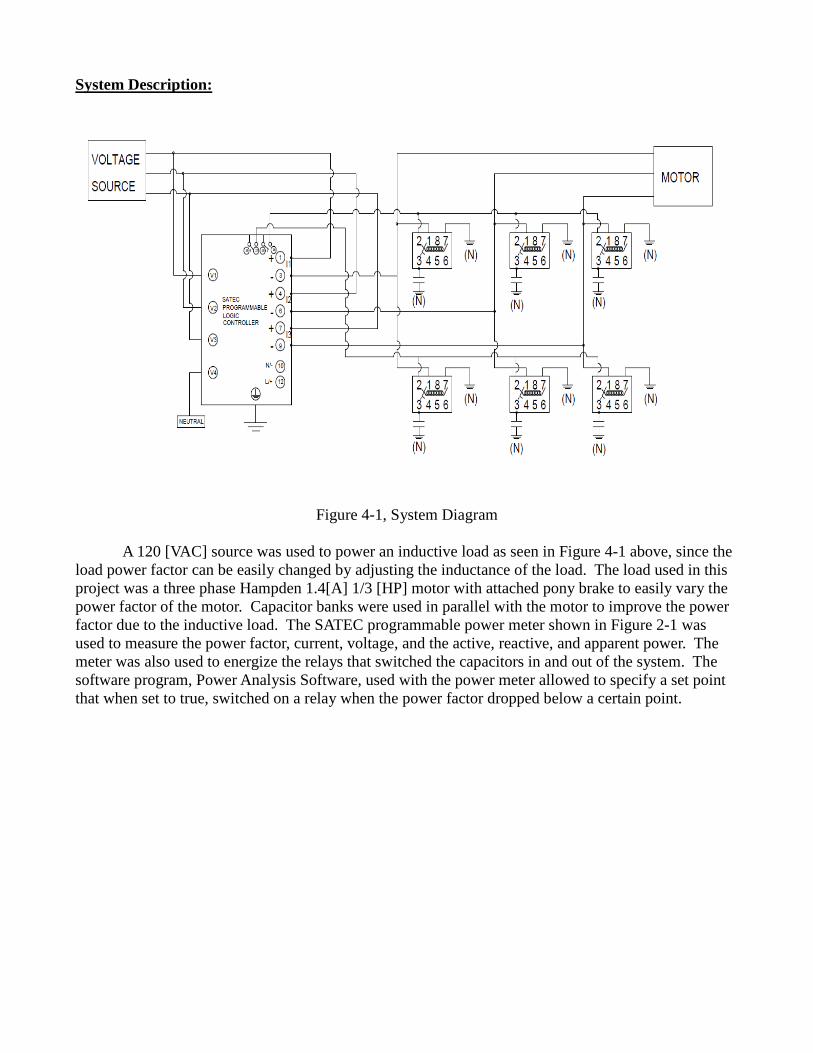
Figure 4-1, System Diagram

A 120 [VAC] source was used to power an inductive load as seen in Figure 4-1 above, since the load power factor can be easily changed by adjusting the inductance of the load. The load used in this project was a three phase Hampden 1.4[A] 1/3 [HP] motor with attached pony brake to easily vary the power factor of the motor. Capacitor banks were used in parallel with the motor to improve the power factor due to the inductive load. The SATEC programmable power meter shown in Figure 2-1 was used to measure the power factor, current, voltage, and the active, reactive, and apparent power. The meter was also used to energize the relays that switched the capacitors in and out of the system. The software program, Power Analysis Software, used with the power meter allowed to specify a set point that when set to true, switched on a relay when the power factor dropped below a certain point.

Equipment List: Hampden Type WRM-100 Three Phase Motor

Figure 6-1, Hampden Motor with Attached Load

Motor is rated at 1.4 [A] 220 [VAC] 1725 RPM 1/3 [HP]. Shown in Figure 6-1, attached is a pony brake load that allows varying the power factor of the motor. The top of the pony brake is cut off, but the load is varied by a knob that is twisted. A force meter is also attached so that efficiency can be measured by calculating the torque of the motor at various loads. A tachometer was also used to measure the RPM output of the motor. The torque was then multiplied by the output speed in radians per second gave the output power of the motor. This output power was divided by input power, which was obtained from meter readings, and multiplied by one hundred to obtain efficiency. A graph of these results was prepared and compared against power factor and is shown on the next page.

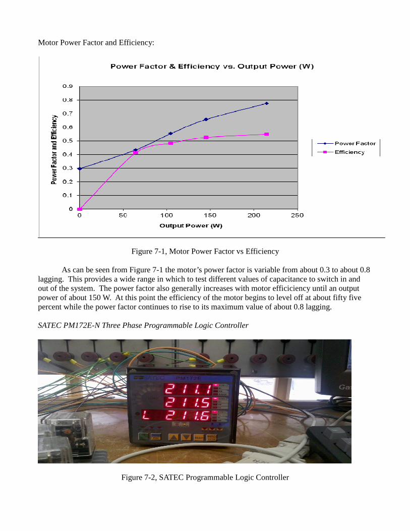
Motor Power Factor and Efficiency:

Figure 7-1, Motor Power Factor vs Efficiency As can be seen from Figure 7-1 the motor’s power factor is variable from about 0.3 to about 0.8 lagging. This provides a wide range in which to test different values of capacitance to switch in and out of the system. The power factor also generally increases with motor efficiciency until an output power of about 150 W. At this point the efficiency of the motor begins to level off at about fifty five percent while the power factor continues to rise to its maximum value of about 0.8 lagging. SATEC PM172E-N Three Phase Programmable Logic Controller

Figure 7-2, SATEC Programmable Logic Controller

The SATEC programmable logic controller was used as the meter for this project along with the energy source used to energize the relays used for switching. The data values taken from the meter for this project are the line to nuetral voltages, active power, power factor, apparent power, reactive power, line currents, and the individual line powers and power factors. The controller is programmed either by the buttons provided on the front of the meter or through SATEC’s free software program, Power Analysis Software (PAS). This software allows the user to program set points that perform a certain action when one or multiple conditions are set. One such action that can be taken is to energize or release realys based on what the power factor of the system is. The software also provides several charts and graphs that either stored data or real time data from the controller. A tutorial of the main functions of the controller is provided at the end of this report. Alternative Controllers: It should be noted that there are other programmable logic controllers available and a lot of them have more than two relay inputs and outputs. These alternative controllers also may have more programming options, such as the ability to set an action when the power factor goes above a certain point instead of only below as is the case for the controller used for this project. Two of the main companies that make these other controllers are Schweitzer Engineering Laboratories and General Electric Company. For this project, this controller was graciously loaned from Ameren Corporation so it was the controller that was used. The two controllers shown in Figure 8-1 and Figure 8-2 are two examples of alternative controllers that can be used. The controller shown in Figure 8-1 is a Schweitzer Engineering Laboratory 734B Logic Controller. The controller shown in Figure 8-2 is a General Electric PM35 Logic Controller.

Figure 8-1, SEL PLC Figure 8-2, GE PLC

Potter & Brumfield KRPA-11AG-120 Power Relays Figure 9-1 shows the relays that were used to switch the capacitor banks in and out of the circuit. These relays were controlled by the SATEC PLC and were also generously donated by Ameren Corporation. Figure 9-2 is a side view of the relays.

Figure 9-1, Top View of Relay Figure 9-2, Side View of Relay Capacitor Banks These were the capacitor banks used in this project. There are two values of steps that could be used with the range of capacitance per step that was able to be switched into the system was 1.6uF to 50uF. Figure 9-3 shows a maximum value of 50uF capacitor bank with switches that enable different values of capacitance to be configured. Figure 9-4 switches in the same way, but contains only a maximum capacitance of 40uF.

Figure 9-3, 50uF Capacitor Bank Figure 9-4, 40uF Capacitor Bank

Damping Resistors: Damping resistors are placed in series with the capacitors that are being switched into the system to limit the inrush current that occurs. Figure 10-1 shows a resistor valued at 25 ohms. This inrush current occurs because when a capacitor is switched on initially it looks like a short circuit and draws very large currents for a short amount of time. Normally in a power factor correction system these resistors are only placed in series with the capacitors for a very short amount of time to limit these inrush currents and avoid excessive power losses due to the resistors. After this short amount of time, the resistors are switched out of the circuit and the capacitors remain in parallel with the load. Due to the limited about of relay outputs available on the controller used for this project, the damping resistors were kept in series with the capacitors and losses were calculated. Current through 10uF Capacitor Power Losses Current through 20uF Capacitor Power Losses Current through 30uF Capacitor Power Losses

Figure 10-1, Damping Resistor 25 ohms

][6159.84450395.06159.84433.266

0120AI °∠=

°−∠°∠=

][07139.525*)450395.0( 22 WRIP ===

][3252.79889119.03252.79965.134

0120AI °∠=

°−∠°∠=

][7633.19 WP =

][2121.7430597.12121.748857.91

0120AI °∠=

°−∠°∠=

][639.42 WP =

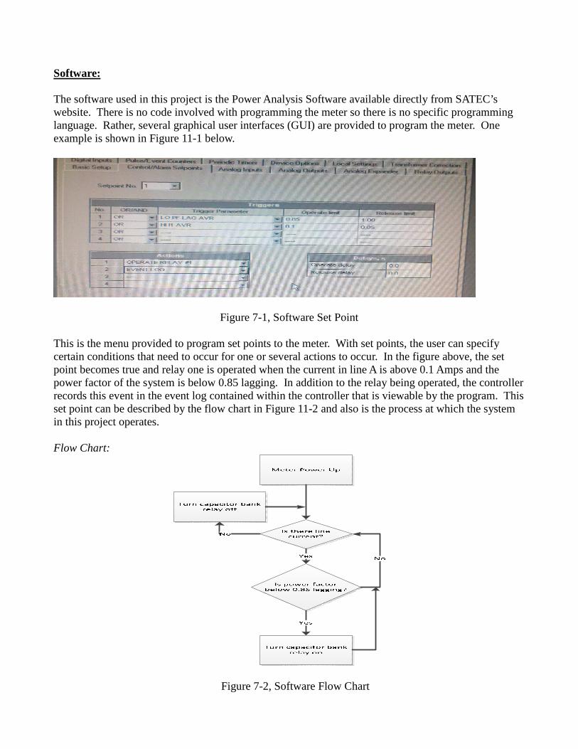
Software: The software used in this project is the Power Analysis Software available directly from SATEC’s website. There is no code involved with programming the meter so there is no specific programming language. Rather, several graphical user interfaces (GUI) are provided to program the meter. One example is shown in Figure 11-1 below.

Figure 7-1, Software Set Point

This is the menu provided to program set points to the meter. With set points, the user can specify certain conditions that need to occur for one or several actions to occur. In the figure above, the set point becomes true and relay one is operated when the current in line A is above 0.1 Amps and the power factor of the system is below 0.85 lagging. In addition to the relay being operated, the controller records this event in the event log contained within the controller that is viewable by the program. This set point can be described by the flow chart in Figure 11-2 and also is the process at which the system in this project operates. Flow Chart:

Figure 7-2, Software Flow Chart

Beginning at the top of Figure 7-2 once the controller powers up, it checks to see whether a load is present by checking whether there is any line current in the system and if no current is present, any relays that are on are turned off and this check is repeated. If there is current then the meter checks to see if the system is running at a power factor below 0.85 lagging and if it is the relays are energized and the capacitor banks are switched into the system. The check for line current and a lagging power factor continue until the meter is powered down.

Results: To determine what value of capacitance needed to be switched into the system, a theoretical model of the motor was made. The magnitude of impedance of the motor was found by dividing the voltage by the current of a single line of the motor. The phase angle of the impedance was found by taking the inverse cosign of the power factor of the motor. The impedance of the motor was recorded at four different power factors, 0.3, 0.45, 0.6, and 0.78 lagging. Five different values of capacitances were each added with each of the different power factors. Once the model of the motor was developed, the damping resistor and capacitor bank were added in parallel and the equivalent impedance was found. This allowed a calculation of the phase angle of the total impedance and the cosign of this angle was taken to obtain a source power factor. A table, Figure 12-1, and a graph, Figure 12-2, are shown below. Any value above one should be subtracted from two and taken as a leading power factor.

0.3 0.45 0.6 0.78

10uF 0.609445 0.74704 0.855108 0.933201

15uF 0.873233 0.928109 0.964573 0.983411

20uF 0.999937 0.999926 1.00002 0.999972

30uF 1.13754 1.09493 1.06663 1.03199

40uF 1.21777 1.17129 1.13211 1.07689

Figure 12-1, Theoretical Values

Figure 12-2, Theoretical Graph

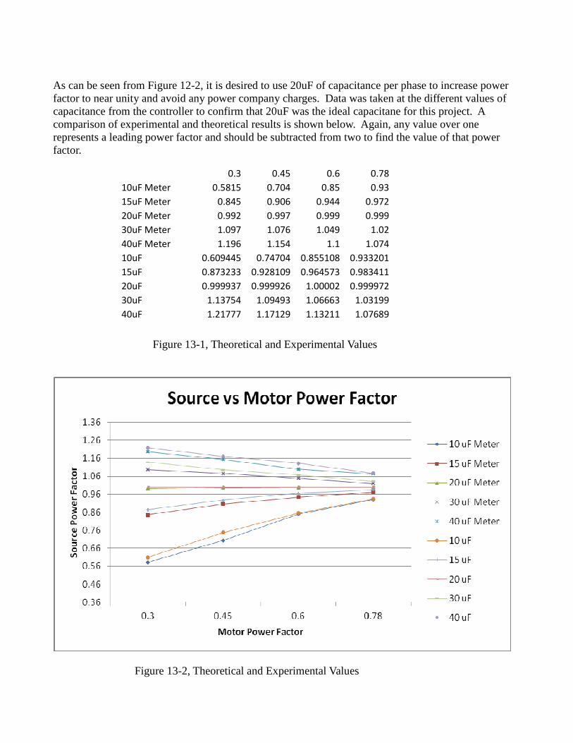
As can be seen from Figure 12-2, it is desired to use 20uF of capacitance per phase to increase power factor to near unity and avoid any power company charges. Data was taken at the different values of capacitance from the controller to confirm that 20uF was the ideal capacitane for this project. A comparison of experimental and theoretical results is shown below. Again, any value over one represents a leading power factor and should be subtracted from two to find the value of that power factor.

Figure 13-1, Theoretical and Experimental Values

Figure 13-2, Theoretical and Experimental Values

0.3 0.45 0.6 0.78

10uF Meter 0.5815 0.704 0.85 0.93

15uF Meter 0.845 0.906 0.944 0.972

20uF Meter 0.992 0.997 0.999 0.999

30uF Meter 1.097 1.076 1.049 1.02

40uF Meter 1.196 1.154 1.1 1.074

10uF 0.609445 0.74704 0.855108 0.933201

15uF 0.873233 0.928109 0.964573 0.983411

20uF 0.999937 0.999926 1.00002 0.999972

30uF 1.13754 1.09493 1.06663 1.03199

40uF 1.21777 1.17129 1.13211 1.07689

A final picture of the system is shown in Figure 14-1. The motor seen on the right has the attached pony brake and is currently running. This is shown by the controller in between the two capacitor banks. The controller is currently measuring the apparent power, power factor, and active power. Behind the controller is the fused power source, with several neutral points being used and a ground. The damping resistors are right in front of the capacitor banks, but connected in series with them. Finally, Power Analysis Software can be seen on the computer displaying real time values of the system including individual active powers, line voltages, and individual line power factors.

Figure 14-1, Picture of Current System

Satec PM172-N Programmable Logic Controller and Power Analysis Software Tutorial: Powering Controller and Communicating with Computer: To power up the meter, a 120 [VAC] source is needed along with a ground and neutral connection. These are connected to ports 10, 12 and ground as demonstrated in Figure 9-1 below.

Figure 9-1, Terminal Connections

When connecting the controller to line voltage and current there are several different wiring modes available and depending on which are available the controller will need to be told which ones to use.

These settings can be set in the meter or the software program. One such configuration and the one used in this project can be seen in Figure 10-1.

Figure 10-1, 4LL3 or 4Ln3 Wiring Configuration

Note in the above diagram that current transformers are used. The controller can be told what ratio of potential and current transformers are used if not directly connecting the controller to line power. The controller is able to be programmed from the front to do and see anything that would be set or seen in the software program. As there are easily over two hundred settings and measurements that can be viewed, this tutorial will only cover the settings used in this project and will only cover which method was used to configure these settings. The rest can be found in the manual downloaded from the SATEC website. The most common way to connect the controller to a computer to view data or configure settings is through a serial port connection, although an adapter can be bought to communicate over ethernet or dial up. This serial port connection also needs to use a null modem cord and not a straight modem cord, otherwise the controller will not respond to computer commands. When using the Power Analysis Software, the user can create multiple databases corresponding to each controller connected. For this project since only one controller was used, there was no need to create multiple databases and remained with the default database. To set up communications with the controller press Configuration from the Tools menu at the top and select the site database to be used along with the model number of the controller, which for this project was PM172-N.

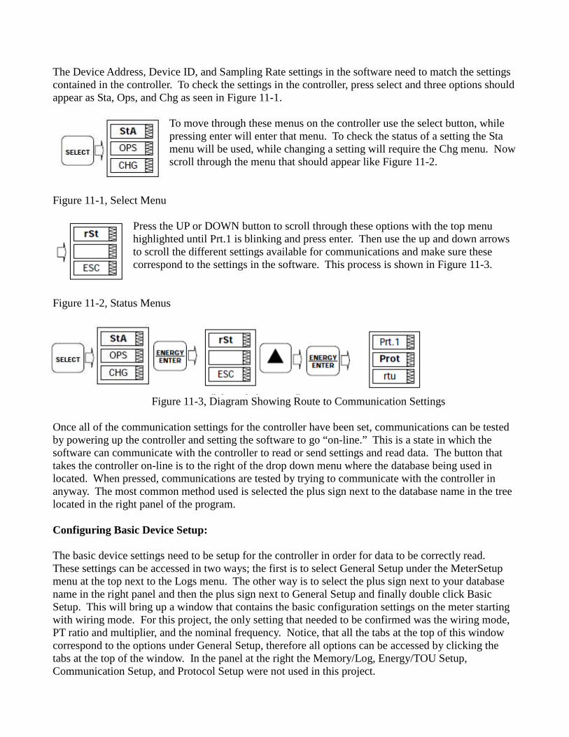
The Device Address, Device ID, and Sampling Rate settings in the software need to match the settings contained in the controller. To check the settings in the controller, press select and three options should appear as Sta, Ops, and Chg as seen in Figure 11-1.

To move through these menus on the controller use the select button, while pressing enter will enter that menu. To check the status of a setting the Sta menu will be used, while changing a setting will require the Chg menu. Now scroll through the menu that should appear like Figure 11-2.

Figure 11-1, Select Menu Press the UP or DOWN button to scroll through these options with the top menu highlighted until Prt.1 is blinking and press enter. Then use the up and down arrows to scroll the different settings available for communications and make sure these correspond to the settings in the software. This process is shown in Figure 11-3.

Figure 11-2, Status Menus

Figure 11-3, Diagram Showing Route to Communication Settings

Once all of the communication settings for the controller have been set, communications can be tested by powering up the controller and setting the software to go “on-line.” This is a state in which the software can communicate with the controller to read or send settings and read data. The button that takes the controller on-line is to the right of the drop down menu where the database being used in located. When pressed, communications are tested by trying to communicate with the controller in anyway. The most common method used is selected the plus sign next to the database name in the tree located in the right panel of the program. Configuring Basic Device Setup: The basic device settings need to be setup for the controller in order for data to be correctly read. These settings can be accessed in two ways; the first is to select General Setup under the MeterSetup menu at the top next to the Logs menu. The other way is to select the plus sign next to your database name in the right panel and then the plus sign next to General Setup and finally double click Basic Setup. This will bring up a window that contains the basic configuration settings on the meter starting with wiring mode. For this project, the only setting that needed to be confirmed was the wiring mode, PT ratio and multiplier, and the nominal frequency. Notice, that all the tabs at the top of this window correspond to the options under General Setup, therefore all options can be accessed by clicking the tabs at the top of the window. In the panel at the right the Memory/Log, Energy/TOU Setup, Communication Setup, and Protocol Setup were not used in this project.

Viewing Data: When the controller is initially power on, the line to neutral voltages are displayed which is shown by the L present in the bottom left corner. To scroll through the measurements, the up and downs arrows are used and if the down arrow is pressed the line to line voltages are displayed which is shown by a P. The next set of measurements will be the line currents and the next measurements are the apparent power, power factor, and real power respectively. The last set of menus displays the neutral line current, frequency, and the reactive power. These values can also be viewed in the software along with many other data. To view real time values in chart or graph form, go to the monitor menu at the top and scroll over RT data monitor. This will list all the available chart or graph types that can be read. The ones used in the project are the Data Set 1 Real Time Measurements and Data Set 2 Average Measurements. Initially, the chart form of data is shown, but graph form can be displayed by pressing the first top left button that is called data trend when hovered over. When in chart form, the data displayed can be changed for any data set by pressing the fifth button from the left that when hovered over is called data set. For changing data values displayed in the graph, the fifth button from the left is pressed. An event log that displays user defined events, when set points are set, and when the controller is powered up or down. This event log can be found by selecting the event log under the logs menu at the top. This event log is very useful for viewing when a set point has been activated or released and when the set points were sent to the controller. Programming Set Points: The set point menus can be accessed from the same window that was used to access the Basic Setup Menu. Click the Control/Alarm Setpoints tab and there should be a drop down menu where the set point number is chosen, a triggers box where logic operators, trigger parameters, and operate and release limits are set, an actions box where actions to take when the set point becomes true, and a box for operate and release delays. For this project the three important trigger parameters that were used are the LO PF LAG AVR, LO PF LEAD AVR, and HI I1 AVR. The operate parameter for a lagging power factor was set at 0.85 while the release limit was at 1.0. This was anded with the current parameter to ensure the relays only switch when line current is present. The set point became true when the power factor at the source fell below 0.85 lagging and line current is present. The actions taken were OPERATE RELAY #1 and EVENT LOG. The operate relay action sent a signal out of the relay output #1 from the controller and the event log action logged that the set point was evaluated to be true. To send the current configuration to the controller there is a send button in the bottom left of the window. Configurations can be saved and loaded into the databases mention earlier by pressing the save as button and selecting the database pertinent to the controller being programmed.