THESETHESEEn vue de l’obtention du

DOCTORAT DE L’UNIVERSITE DE TOULOUSE

Delivre par : l’Universite Toulouse 3 Paul Sabatier (UT3 Paul Sabatier)Cotutelle internationnale Hanoi Institute of Physics

Presentee et soutenue le 01/11/2014 par :PHAM Tuan Anh

Observations millimetriques/submillimetriques de galaxies lentilleesgravitationellement a haut redshift

JURYM. Peter von BALLMOOS IRAP, Observatoire de

Midi-PyreneesPresident

M. Johan RICHARD CRAL, Observatoire de Lyon RapporteurM. NGUYEN Quang Rieu LERMA, Observatoire de Paris RapporteurM. Frederic BOONE IRAP, Observatoire de

Midi-PyreneesDirecteur de these

M. Pierre DARRIULAT VATLY, Hanoi Directeur de theseM. DINH Van-Trung IOP, Hanoi ExaminateurM. PHAN Bao Ngoc HCMIU, Ho Chi Minh City Invite

Ecole doctorale et specialite :SDU2E : Astrophysique, Sciences de l’Espace, Planetologie

Unite de Recherche :Institut de Recherche en Astrophysique et Planetologie (UMR 5277)

Directeur(s) de These :Frederic BOONE et Pierre DARRIULAT

Rapporteurs :Johan RICHARD et NGUYEN Quang Rieu

ii

Acknowledgements

I express my deep gratitude to my supervisors in Toulouse, Dr. Frédéric Boone, and in Ha Noi, Pr. Pierre Darriulat, for their constant support. In particular, I would like to thank Frédéric for introducing me to this extremely exciting field of astrophysics and for his explaining things to me when I was in Toulouse. This thesis would have not been possible without him. I would like to thank Pierre for his utmost contribution to get me involved in the game, for always beside me to learn together and to help me get through. His un-tired effort is an example for me to pursuit this kind of study.

I thank my colleagues in Ha Noi and in Toulouse for the friendly working atmosphere to which they contribute and their many helpful advices. In particular, I would like to thank Dr. Pham Tuyet Nhung for her patient guidance in data analysis with PAW, for her following my progress and for her encouragement. I am also very grateful to Do Thi Hoai for her contribution to the work on gravitational lensing. I would also like to thank Dr. Pham Ngoc Diep, Dr. Pham Ngoc Dong, Dr. Nguyen Thi Thao, Nguyen Thi Phuong for sharing the same interest, for their encouragements and their help.

On this occasion, I would like to thank Pr. Nguyen Quang Rieu for his encouragement and support to get me involved in the field of radio astronomy. I would like to thank Pr. Dinh Van Trung for his useful comments/suggestions on various occasions in which he took part. I would also like to thank Eric Jullo for his very patient explanations on how to use LENSTOOL properly. I express my gratitude to professors/lecturers to let me take part in wonderful schools about mm radio astronomy in Granada for single dish observation and in Grenobe for interferometer system, in particular to Pr. Frédéric Gueth for clearly explaining how to work in uv plane, to Pr. Axel Weiss for guiding me on how to observe with the IRAM 30m dish, to Dr. Pierre Gratier and Dr. Sebastien Bardeau for their help of using GILDAS. I am indebted to the French Embassy in Ha Noi for the allocation of a fellowship that made it possible for me to travel to and live in Toulouse during my three four-month stays. Financial and/or material support from the Université Paul Sabatier, the Institute for Nuclear Studies and Technology, NAFOSTED, the World Laboratory, Rencontres du Vietnam and Odon Vallet fellowships is gratefully acknowledged.

On a private side, I express my gratitude to my family for their continuous support and encouragement. They are always behind me in whatever step I make.

iii

Abstract

The study of the formation and evolution of galaxies in the early Universe is one of the most active lines of research in contemporary astrophysics.

One distinguishes between star-forming galaxies − typically blue, dense

and dusty spirals including a fast rotating disk of young stars and a halo of low metallicity stars − and star-not-forming galaxies − typically red ellipticals, made of old stars and containing little to no dust. Both types usually have a black hole in their centre, with masses ranging from a few millions to a few billions solar masses, and are contained in large dark matter haloes, the more so the more massive they are. Mergers play an important role in the evolution of structures in the Universe, major mergers between two spirals producing elliptical galaxies.

At large redshifts (z), we observe the early Universe. In addition to star

emission in the visible, we learn about the dust content and the Star Formation Rate (SFR) from the Far Infrared (FIR) continuum distribution, about the gas content from molecular lines (mostly CO), about Active Galactic Nuclei (AGN) from the radio and X ray emission of their jets. At all wavelengths, the exploration of the early Universe has recently made spectacular progress. The star formation rate density and stellar mass build-up have been quantified back to 1 Gyr of the Big Bang. The comoving SFR density starts with a steady rise from z~10 to 6 when light from the first galaxies re-ionizes the neutral intergalactic medium. It then peaks at z~3 to 1, in what is known as the epoch of galaxy assembly during which about half of the stars in the present day Universe form. Last comes the order of magnitude decline from z~1 to 0.

The present work studies the host galaxy of a z=2.8 quasar, RX J0911,

namely a galaxy having an active black hole in its centre, seen at the epoch of galaxy assembly. It uses data collected at the Plateau de Bure Radio Interferometer at the frequency corresponding to the red-shifted emission of the CO(7-6) molecular rotation line. Observation of the line probes the gas in the galaxy, observation in the continuum probes the dust. The intensity of the line tells us about the size and physical properties of the gas reservoir of the galaxy, its width and profile tell us about its dynamics and therefore kinetic energy content. The intensity of the continuum provides important information on the star formation rate, which is itself associated with the production of dust.

As is often the case with the observation of remote galaxies, RX J0911 is

gravitationally lensed by a foreground galaxy, producing four resolved images. At the same time as the large magnification, ~20, offered by gravitational lensing

iv

eases considerably the observation of the prominent features of the galaxy, it significantly complicates the interpretation of the data. As usual, large magnifications are obtained when the source is near the lens caustic where the distortion of the image is maximal. This is the case of RX J0911, the host galaxy of which overlaps the lens caustic.

The work is organised in 5 chapters and 4 annexes. The first chapter starts with a general introduction to the subject covering

the main topics addressed in the thesis: galaxies in the early universe, quasars at high redshift, gravitational lensing and radio interferometry. It borrows much from textbooks, lectures, reviews and encyclopaedia articles. It continues with a review of earlier observations of RX J0911, including Hubble Space Telescope observations of the quasar in the visible and near infrared, X ray data and earlier molecular data (mostly CO). A description of the lens and of the galaxy cluster in which it is contained sets the scene for the gravitational lensing mechanism. The chapter closes with a description of data collection at Plateau de Bure and data reduction from raw data into visibilities in the Fourier plane and sky maps.

The second chapter provides a detailed study of the gravitational lensing

scenario. It makes use of two different lensing potentials (1 and 2) allowing for a comparison between their predictions and for an estimate of the most important systematic uncertainties attached to the results. One of the potentials combines an elliptic lens with an external shear term mimicking the presence of the galaxy cluster and of a small satellite galaxy. Its treatment is fully home made, with a code including the explicit resolution of the lens equation. The other uses a more sophisticated code, available for public use, called LENSTOOL. Instead of using a phenomenological shear term, it describes the lensing effect of the cluster by a fictitious lens located at its centre of mass. As the source is very close, in the sky plane, to the main lensing galaxy, the effect of the cluster is only a perturbation and it is interesting to study how the two approaches differ in their results. The method of resolution of the lens equation is spelled out in detail and particular attention is given to the proximity of the lens caustic. Indeed, the host galaxy of RX J0911 overlaps the lens caustic, implying that part of it gives only two images and the other part four images, with maximal distortion at the boundary. As the caustics obtained from the two lensing potentials differ slightly, so do the distortions imposed on the images, generating a source of systematic uncertainties that is thoroughly explored. General features characteristic of sources located near the lens caustic are described, in particular for quadruply imaged quasars and for what concerns velocity gradients and image brightness ratios.

The third chapter applies what precedes to a model of the host galaxy of

RX J0911. While occasionally displaying sky maps, most of the work is done in

v

the uv plane where a more rigorous treatment can be applied. The agreement between observations and model predictions is quantified by the evaluation of a χ2, which is minimized by adjusting the model parameters in order to best fit the data. The reliability of the method is discussed together with a critical evaluation of the sources of uncertainties contributing to the result.

The source size is evaluated using a model of the source brightness

including a uniform central region and Gaussian edges, both elliptical with a ratio λ2 between the major and minor axes. The overall size is defined by a parameter ρ, the square root of the mean square radius, and the orientation by a position angle α. Particular cases where the brightness distribution is purely uniform or Gaussian and where the shape is circular have been studied. Both potentials 1 and 2 are used as lens models and the difference between their predictions gives an estimate of systematic uncertainties. The best fit to the line data is given by the following set of parameters: ρ=104±16 mas, λ=1.60+0.35

−0.18 and α=111o±9o. The hypothesis of a point source is rejected at the level of 6 standard deviations, that of a circular source at the level of 3.3 standard deviations. This result is consistent with the measured B/A ratio of image brightness. However, including a more precise earlier measurement, B/A=21±1%, implies ρ=120±15 mas. Combining all results together gives ρ=106±15 mas and B/A=0.19±0.01.

Evidence for a velocity gradient on the line has been found at the level of

4.5 standard deviations. While potential 2 produces a best-fit source position closer to the caustic than potential 1 does, it also implies larger magnifications and, as a result, a smaller source size. However, potentials 1 and 2 make remarkably similar predictions in terms of source ellipticity and velocity gradient. Fits performed on the clean and dirty maps have illustrated the difficulties of dealing properly with the noise in such cases and have added further confidence to the results obtained in the uv plane. The best fit to the continuum data, using the same values of λ and α as found on the line, gives ρ=32±16 mas, implying that the source is resolved at the level of only 2 standard deviations.

The fourth chapter gives an interpretation of the above results. It starts with a general introduction to galaxy formation and evolution, with particular emphasis on recent FIR and CO data.

The line luminosity is obtained from the integrated line flux, Sline∆ν,

evaluated on the clean map. A Gaussian fit to the line gives a peak value of 47.6 mJy, a mean velocity of −22±6 kms−1 and a full width at half maximum of 120±14 kms−1 for a continuum level of 4.0±0.5 mJy. The line integrated flux is measured to be 5.0±0.5 Jykms−1 and the continuum 4.4±0.5 mJy. The evaluation of the luminosities is strongly dependent on the values of the magnification adopted as best describing the lensing mechanism. This is by far the main source of

vi

uncertainties. Magnifications of 12±4 are retained on the line, 24±10 in the continuum and 26±10 for the quasar point source. The table below summarizes the main properties.

RX J0911 data

Lens potential P1 P2 Retained

Magnification (point source) 17.4 35.9 26±10 Magnification (line) 9.4±0.7 16.0±1.1 12±4 Magnification (continuum) 15.4±2.2 33.9±4.8 24±10 L’CO(7-6) [109K km s–1pc2] 3.9±0.8 2.3±0.5 3.1±1.0 L’CO(1-0) [109K km s–1pc2] 4.9±1.0 2.9±0.6 3.9±1.3

Continuum [mJy] 0.31±0.08 0.14±0.04 0.20±0.09 MH2 [109 MSun] 3.9±0.8 2.3±0.5 3.1±1.0 SFR [MSun/yr] ~360 ~160 ~230

Depletion rate [107 yr] 1.1 1.4 1.3 Dust mass [108 MSun] ~1.3 ~0.6 ~0.8

Mdyn [109 MSun] 4.7±1.4 4.7±1.4 4.7±1.4 ρ (line) [arcsec] 115±13 81±9 106±15

ρ (continuum) [arcsec] 51±15 24±10 39±18 Details of the calculations are given in the first two annexes. The main

uncertainty on the gas mass remains the value of the magnification, which is nearly halved when using potential 1 rather than potential 2, meaning twice as high a gas mass. Even so, the molecular gas mass is quite small in comparison with other quasar hosts and lies at the low end of their observed range. Possible biases that might have caused a gross underestimate are thoroughly explored but the low gas mass of RX J0911, when compared with other high-z objects, whether quasar hosts or SMGs, is unescapable. The spectral energy distribution, the knowledge of which is necessary to calculate the star formation rate, is not strongly constrained by available data and its evaluation is accordingly somewhat arbitrary, having to rely on general knowledge obtained from other galaxies to obtain a total FIR luminosity LFIR=320 µ–11011LSun, where µ is the magnification. Similarly, the evaluation of the dust mass from the continuum luminosity is subject to major uncertainties. The RX J0911 star formation efficiency is seen to be on the high side of all galaxies, whether low-z or high-z and both CO and FIR luminosities are at the low end of the high-z population, at the border between high-z and low-z quasar hosts and SMGs. It is as if RX J0911 had exhausted much of its gas after a period of intense star formation.

With respect to other quasar hosts, RX J0911 has an outstandingly small

line width. While this observation directly rules out any contribution from important virial dispersion, it suggests that the gas is in the form of a rotating disk

vii

seen face on. This is however in contradiction with the elliptic morphology that has been measured, requiring a critical assessment of the uncertainties attached to the associated measurements. Using the full band X-ray luminosity density of RX J0911 that has been measured by Fan et al. 2009 one obtains further evidence for an abnormally low dynamical mass: while both the gas and dynamical masses are low with respect to other quasar hosts, this is not to be blamed on a particularly low black hole mass.

The last chapter summarizes the work and opens a window on the

future. The detailed study of the host galaxy of a remote quasar, observed at

millimetre wavelengths, has illustrated some of the most remarkable properties of far away galaxies and of their evolution in the early Universe when most of the existing stars were being formed. The observation of CO and continuum emissions has taken advantage of the magnification offered by gravitational lensing and of the quality of the Plateau de Bure interferometer in terms of sensitivity and resolution, allowing for resolving the source in space and for a precise measurement of the observed molecular line.

A careful study of the properties of gravitational lensing for sources close to the caustic has shed light on its most remarkable properties et can be used as a guide for future observations of galaxies in similar situations of gravitational optics. The data analysed here have illustrated the complications that result and have made it possible to evaluate the associated sources of uncertainties, in particular concerning the strong dependence of the magnification on the source dimensions.

As the CO(7-6) line stands out clearly above continuum, reliable measurements of the luminosities related to the gas and to the dust have been possible. A detailed study of the images has made it possible to resolve the source in space and, for what concerns the gas volume, to evaluate its morphology – size, ellipticity, position angle – and to provide evidence in favour of a velocity gradient. A remarkable property of the CO(7-6) emission is its extremely narrow line width, implying a small dynamic mass consistent with independent evaluations of the gas and dust masses. The large star formation efficiency suggests that the galaxy has exhausted a large part of its gas reserve following a period of intense star formation and lies now at the boundary between high z and low z quasar hosts.

The recent start-up of ALMA, offering substantially improved

performance in terms of sensitivity and resolution with respect to Plateau de Bure, has led us to propose the observation of a quasar host similar to RX J0911,

viii

gravitationally lensed into six images with a magnification of order hundred. As explained in the annexes 3 and 4, a resolution of ~50 pc could be reached in only two hours of observation of the CO(9-8) line. The water line could also be detected, offering useful information on the FIR luminosity.

The observation of high z quasar hosts has a rich future in front of it and

will undoubtedly significantly contribute to our understanding of the formation and evolution mechanisms of structures in the early Universe. We hope to be able to take an active part in this exploration and make good use of the experience gained in the study of RX J0911.

ix

Résumé

L’étude de la formation et de l’évolution des galaxies dans les premiers temps de l’Univers constitue l’une des voies de recherches les plus actives de l’astrophysique contemporaine.

On a coutume de distinguer les galaxies à fort taux de formation d’étoiles −

typiquement des spirales bleues, denses et riches en poussière, comportant un disque d’étoiles jeunes en rotation rapide et un halo d’étoiles de métallicité faible − des galaxies sans formation d’étoiles − typiquement des elliptiques rouges faites d’étoiles anciennes et ne contenant que peu de poussière, voire pas du tout. Les deux familles ont un trou noir à leur centre, de masses allant de quelques millions à quelques milliards de masses solaires, et baignent dans de grands halos de matière noire, d’autant plus grands qu’elles sont plus massives. Les collisions résultant en la réunion de deux galaxies jouent un rôle important dans l’évolution des structures dans l’Univers, les collisions de ce type entre deux spirales massives produisant les galaxies elliptiques.

À grand décalage vers le rouge (z), nous observons l’univers à ses débuts.

Outre l’émission stellaire dans le visible, le continu de l’infrarouge lointain nous renseigne sur la quantité de poussière et le taux de formation d’étoiles, les raies moléculaires (essentiellement CO) sur la quantité de gaz. Les émissions X et radio des jets des noyaux galactiques actifs est une source additionnelle d’information. L’exploration de l’Univers à ses débuts a fait récemment des progrès spectaculaires dans tous les domaines de longueur d’onde. La densité du taux de formation d’étoiles et la croissance de la masse stellaire sont maintenant mesurées jusqu’à un milliard d’années après le Big Bang. La première commence par augmenter progressivement entre z~10 et z~6 , époque à laquelle le rayonnement émis par les premières galaxies ré-ionise le milieu interstellaire neutre. Elle atteint ensuite sa valeur maximale à z~3, ce qu’on appelle l’époque d’assemblage des galaxies, lors de laquelle près de la moitié des étoiles existant aujourd’hui se sont formées. La phase finale est une décroissance de près d’un ordre de grandeur entre z~1 et z=0.

La présente étude porte sur la galaxie hôte d’un quasar à z=2.8, RX J0911,

abritant par conséquent un trou noir actif en son centre, à l’époque d’assemblage des galaxies. Elle fait usage de données collectées à l’Interféromètre Radio du Plateau de Bure à une fréquence correspondant à l’émission de la raie moléculaire de rotation CO(7-6) décalée vers le rouge par effet Doppler. L’observation de la raie sonde le gaz dans la galaxie, celle du continu sonde la poussière. L’intensité de la raie nous renseigne sur la taille et les propriétés physiques du volume de gaz, sa largeur et son profil sur ses propriétés dynamiques et son contenu énergétique.

x

L’intensité du continu fournit des renseignements importants sur le taux de formation d’étoiles qui est étroitement lié a la production de poussière.

Comme c’est souvent le cas pour l’observation de galaxies lointaines, RX

J0911 est lentillé gravitationnellement par une galaxie plus proche, avec formation de quatre images séparées. Le grandissement, de l’ordre d’un facteur 20, augmente considérablement la sensibilité du processus de détection mais, en même temps, complique grandement l’interprétation des données. Les grandissements les plus importants sont obtenus lorsque la source est proche de la caustique où la distorsion des images est maximale. Tel est le cas de RX J0911 dont la galaxie hôte chevauche la caustique.

L’ouvrage est construit en cinq chapitres et quatre annexes. Le premier chapitre débute sur une introduction générale aux sujets traités

dans le corps de la thèse: galaxies lointaines, quasars à haut décalage vers le rouge, lentillage gravitationnel et interférométrie radio. Elle emprunte beaucoup à des ouvrages généraux, des cours, des articles d’encyclopédie et des articles de revue. Sont ensuite passées en revue les observations faites antérieurement sur RX J0911, comprenant celles du quasar dans le visible et l’infrarouge proche avec le Hubble Space Telescope, des données dans le spectre X et des mesures antérieures d’émission moléculaire (essentiellement CO). Suit une description du système de lentillage, la galaxie-lentille et l’amas dont elle fait partie. Le chapitre se termine sur une description de la collection de données au Plateau de Bure et de la réduction des données brutes en un ensemble de visibilités dans le plan de Fourier puis de cartes de brillance dans le ciel.

Le second chapitre présente une étude détaillée du scénario de lentillage

gravitationnel. Il utilise deux potentiels de lentillage distincts (1 et 2) permettant de comparer leurs prédictions et d’obtenir ainsi une estimation des incertitudes systématiques les plus importantes affectant la qualité des résultats. Un des potentiels associe une lentille elliptique à un terme de cisaillement qui rend compte de la présence de l’amas de galaxies et d’une petite galaxie satellite. La résolution de l’équation de lentillage suit une méthode conçue pour le cas présent et utilise un code écrit dans ce but. L’autre potentiel utilise un code plus élaboré, accessible dans le domaine public, LENSTOOL. Son potentiel, au lieu d’utiliser un terme de cisaillement, représente l’effet de l’amas par une source fictive placée au centre de masse. Comme la source est très proche, dans le ciel, de la lentille principale, l’effet de l’amas est une perturbation qu’il est intéressant d’étudier selon ces deux approches distinctes afin d’évaluer de combien leurs prédictions diffèrent. La méthode utilisée pour résoudre l’équation de lentillage est décrite en détail et une attention particulière est réservée aux effets liés à la proximité de la caustique. De fait, la galaxie hôte de RX J0911 chevauche la caustique, ce qui

xi

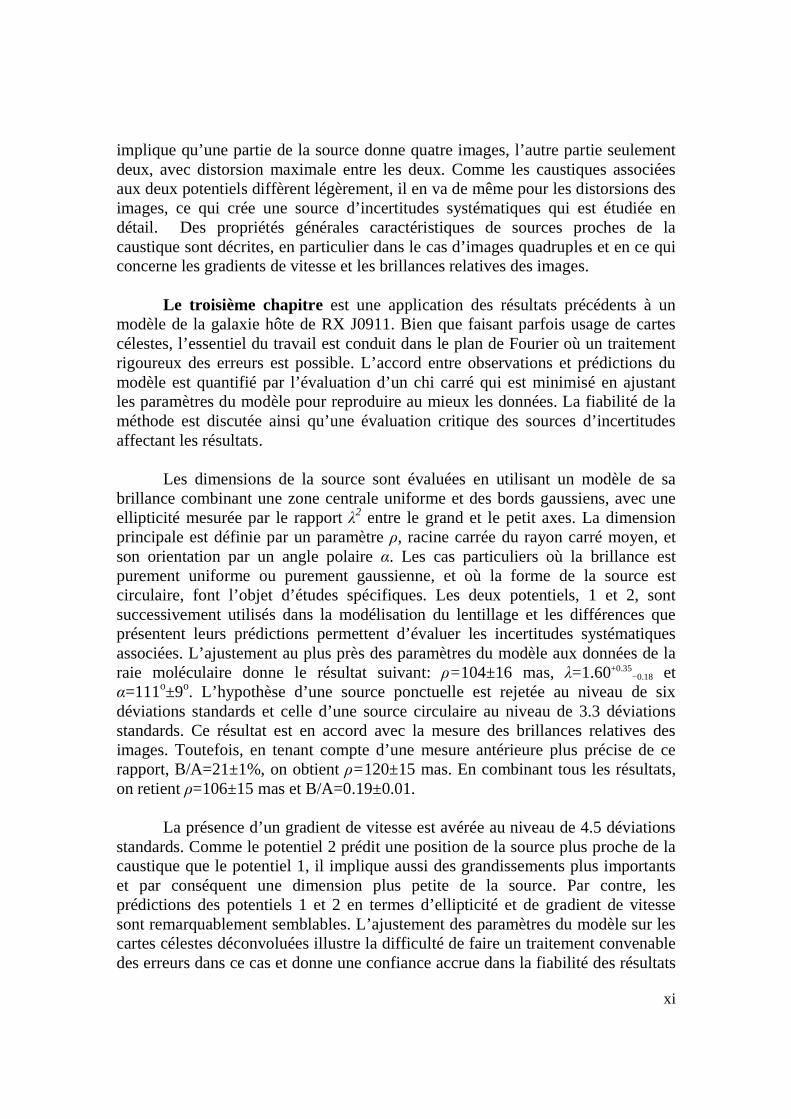
implique qu’une partie de la source donne quatre images, l’autre partie seulement deux, avec distorsion maximale entre les deux. Comme les caustiques associées aux deux potentiels diffèrent légèrement, il en va de même pour les distorsions des images, ce qui crée une source d’incertitudes systématiques qui est étudiée en détail. Des propriétés générales caractéristiques de sources proches de la caustique sont décrites, en particulier dans le cas d’images quadruples et en ce qui concerne les gradients de vitesse et les brillances relatives des images.

Le troisième chapitre est une application des résultats précédents à un

modèle de la galaxie hôte de RX J0911. Bien que faisant parfois usage de cartes célestes, l’essentiel du travail est conduit dans le plan de Fourier où un traitement rigoureux des erreurs est possible. L’accord entre observations et prédictions du modèle est quantifié par l’évaluation d’un chi carré qui est minimisé en ajustant les paramètres du modèle pour reproduire au mieux les données. La fiabilité de la méthode est discutée ainsi qu’une évaluation critique des sources d’incertitudes affectant les résultats.

Les dimensions de la source sont évaluées en utilisant un modèle de sa

brillance combinant une zone centrale uniforme et des bords gaussiens, avec une ellipticité mesurée par le rapport λ2 entre le grand et le petit axes. La dimension principale est définie par un paramètre ρ, racine carrée du rayon carré moyen, et son orientation par un angle polaire α. Les cas particuliers où la brillance est purement uniforme ou purement gaussienne, et où la forme de la source est circulaire, font l’objet d’études spécifiques. Les deux potentiels, 1 et 2, sont successivement utilisés dans la modélisation du lentillage et les différences que présentent leurs prédictions permettent d’évaluer les incertitudes systématiques associées. L’ajustement au plus près des paramètres du modèle aux données de la raie moléculaire donne le résultat suivant: ρ=104±16 mas, λ=1.60+0.35

−0.18 et α=111o±9o. L’hypothèse d’une source ponctuelle est rejetée au niveau de six déviations standards et celle d’une source circulaire au niveau de 3.3 déviations standards. Ce résultat est en accord avec la mesure des brillances relatives des images. Toutefois, en tenant compte d’une mesure antérieure plus précise de ce rapport, B/A=21±1%, on obtient ρ=120±15 mas. En combinant tous les résultats, on retient ρ=106±15 mas et B/A=0.19±0.01.

La présence d’un gradient de vitesse est avérée au niveau de 4.5 déviations

standards. Comme le potentiel 2 prédit une position de la source plus proche de la caustique que le potentiel 1, il implique aussi des grandissements plus importants et par conséquent une dimension plus petite de la source. Par contre, les prédictions des potentiels 1 et 2 en termes d’ellipticité et de gradient de vitesse sont remarquablement semblables. L’ajustement des paramètres du modèle sur les cartes célestes déconvoluées illustre la difficulté de faire un traitement convenable des erreurs dans ce cas et donne une confiance accrue dans la fiabilité des résultats

xii

obtenus dans le plan de Fourier. Dans le continu, en utilisant les valeurs de λ et α obtenues pour la raie, on obtient ρ=32±16 mas: la source n’est résolue qu’au niveau de 2 déviations standards.

Le quatrième chapitre offre une interprétation des résultats précédents. Il débute par une introduction générale aux processus de formation et d’évolution des galaxies, en s’attardant sur les données récentes dans l’infrarouge lointain et en CO millimétrique et submillimétrique.

La luminosité de la raie est obtenue à partir du flux intégré, Sline∆ν, évalué

sur la carte céleste déconvoluée. Une description gaussienne de la raie donne une valeur de 47.6 mJy au sommet, une vitesse moyenne de −22±6 kms−1 et une largeur à mi-hauteur de 120±14 kms−1 pour un niveau dans le continu de ~4.0±0.5 mJy. Le flux intégré sur la raie vaut 5.0±0.5 Jykms−1 et pour le continu 4.4±0.5 mJy. L’évaluation des luminosités dépend fortement des valeurs adoptées pour les grandissements censés décrire au mieux le mécanisme de lentillage. C’est là, et de loin, la cause principale d’incertitude. On retient des grandissements de 12±4 pour la raie, 24±10 dans le continu et 26±10 pour la source ponctuelle qu’est le quasar. Le tableau ci-dessous résume les propriétés les plus importantes.

RX J0911 data

Potentiel de lentillage P1 P2 Valeur retenue

Grandissement (source ponctuelle)

17.4 35.9 26±10

Grandissement (raie) 9.4±0.7 16.0±1.1 12±4 Grandissement (continu) 15.4±2.2 33.9±4.8 24±10 L’CO(7-6) [109K km s–1pc2] 3.9±0.8 2.3±0.5 3.1±1.0 L’CO(1-0) [109K km s–1pc2] 4.9±1.0 2.9±0.6 3.9±1.3

Continu [mJy] 0.31±0.08 0.14±0.04 0.20±0.09 MH2 [109 MSun] 3.9±0.8 2.3±0.5 3.1±1.0 SFR [MSun/yr] ~360 ~160 ~230

Taux de déplétion [107 yr] 1.1 1.4 1.3 Masse de poussière [108

MSun] ~1.3 ~0.6 ~0.8

Mdyn [109 MSun] 4.7±1.4 4.7±1.4 4.7±1.4 ρ (raie) [arcsec] 115±13 81±9 106±15

ρ (continu) [arcsec] 51±15 24±10 39±18 Les détails des calculs sont résumés dans les deux premières annexes.

L’incertitude dominante sur la masse gazeuse est toujours la valeur adoptée pour le grandissement, presque deux fois plus petit pour le potentiel 1 que pour le potentiel 2, donnant une masse gazeuse deux fois plus grande. Même dans ce cas, la masse moléculaire reste très petite en comparaison avec d’autres galaxies hôtes

xiii

de quasars et se tient à l’extrémité inférieure du domaine observé. La présence éventuelle de biais pouvant causer une forte sous-estimation de la masse gazeuse a été explorée mais la basse valeur de la masse gazeuse de la galaxie hôte de RX J0911, comparée à d’autres objets à haut z, galaxies hôtes de quasars ou SMGs, semble inéluctable. La distribution spectrale d’énergie, dont la connaissance est nécessaire au calcul du taux de formation d’étoiles, n’est pas fortement contraint par les données disponibles et son évaluation est par conséquent quelque peu arbitraire: on doit se fier à des propriétés globales obtenues par l’étude d’autres galaxies pour en déduire la luminosité dans l’infrarouge lointain LFIR=320 µ–

11011LSun, où µ est le grandissement. Semblablement, l’évaluation de la masse de la poussière à partir de la luminosité dans le continu est sujette à d’importantes incertitudes. L’efficacité du taux de formation d’étoiles de RX J0911 se situe dans la partie haute de celles d’autres galaxies, quelque soit leur décalage vers le rouge, et les luminosités dans l’infrarouge lointain et en CO se situent dans la partie basse de la population des galaxies lointaines, à la limite entre les SMGs et les galaxies hôtes de quasars, quelque soit la valeur de z.

En comparaison avec d’autres galaxies hôtes de quasars, RX J0911 a une

latgeur de raie anormalement faible. Cette observation exclut d’emblée une contribution importante de dispersion virielle et suggère que le gaz se présente sous la forme d’un disque perpendiculaire à la ligne de vue, ce qui serait en contradiction apparente avec la mesure d’ellipticité décrite plus haut, et ce malgré l’étude critique qui a été faite des incertitudes attachées à cette mesure. En se servant de la densité de luminosité mesurée sur l’ensemble de la bande X de RX J0911, mesurée par Fan et al. 2009, on obtient une autre évidence en faveur d’une masse dynamique anormalement basse: s’il est vrai que la masse gazeuse et la masse dynamique sont faibles par rapport à celles d’autres galaxies hôtes de quasars, ce n’est pas le résultat d’une masse de trou noir particulièrement basse.

Le dernier chapitre résume l’ensemble et ouvre une fenêtre sur l’avenir. Nous en reproduisons l’essentiel ci-dessous.

L’étude détaillée de la galaxie hôte d’un quasar distant, observée en longueurs d’ondes millimétriques, a permis d’illustrer quelques unes des propriétés les plus remarquables des galaxies lointaines et de leur évolution au début de l’histoire de l’Univers, à l’époque où la majorité des étoiles existantes se sont formées. L’observation de l’émission en CO et dans le continu a bénéficié du grandissement offert par le lentillage gravitationnel et de la qualité de l’interféromètre du Plateau de Bure en termes de sensibilité et de résolution qui a permis de résoudre la source dans l’espace et de mesurer avec précision la largeur de la raie moléculaire observée.

xiv

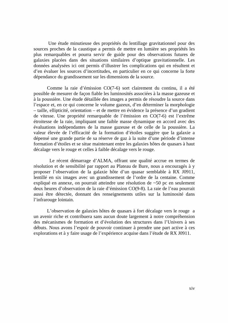
Une étude minutieuse des propriétés du lentillage gravitationnel pour des sources proches de la caustique a permis de mettre en lumière ses propriétés les plus remarquables et pourra servir de guide pour des observations futures de galaxies placées dans des situations similaires d’optique gravitationnelle. Les données analysées ici ont permis d’illustrer les complications qui en résultent et d’en évaluer les sources d’incertitudes, en particulier en ce qui concerne la forte dépendance du grandissement sur les dimensions de la source.

Comme la raie d’émission CO(7-6) sort clairement du continu, il a été

possible de mesurer de façon fiable les luminosités associées à la masse gazeuse et à la poussière. Une étude détaillée des images a permis de résoudre la source dans l’espace et, en ce qui concerne le volume gazeux, d’en déterminer la morphologie – taille, ellipticité, orientation – et de mettre en évidence la présence d’un gradient de vitesse. Une propriété remarquable de l’émission en CO(7-6) est l’extrême étroitesse de la raie, impliquant une faible masse dynamique en accord avec des évaluations indépendantes de la masse gazeuse et de celle de la poussière. La valeur élevée de l’efficacité de la formation d’étoiles suggère que la galaxie a dépensé une grande partie de sa réserve de gaz à la suite d’une période d’intense formation d’étoiles et se situe maintenant entre les galaxies hôtes de quasars à haut décalage vers le rouge et celles à faible décalage vers le rouge.

Le récent démarrage d’ALMA, offrant une qualité accrue en termes de

résolution et de sensibilité par rapport au Plateau de Bure, nous a encouragés à y proposer l’observation de la galaxie hôte d’un quasar semblable à RX J0911, lentillé en six images avec un grandissement de l’ordre de la centaine. Comme expliqué en annexe, on pourrait atteindre une résolution de ~50 pc en seulement deux heures d’observation de la raie d’émission CO(9-8). La raie de l’eau pourrait aussi être détectée, donnant des renseignements utiles sur la luminosité dans l’infrarouge lointain.

L’observation de galaxies hôtes de quasars à fort décalage vers le rouge a

un avenir riche et contribuera sans aucun doute largement à notre compréhension des mécanismes de formation et d’évolution des structures dans l’Univers à ses débuts. Nous avons l’espoir de pouvoir continuer à prendre une part active à ces explorations et à y faire usage de l’expérience acquise dans l’étude de RX J0911.

xv

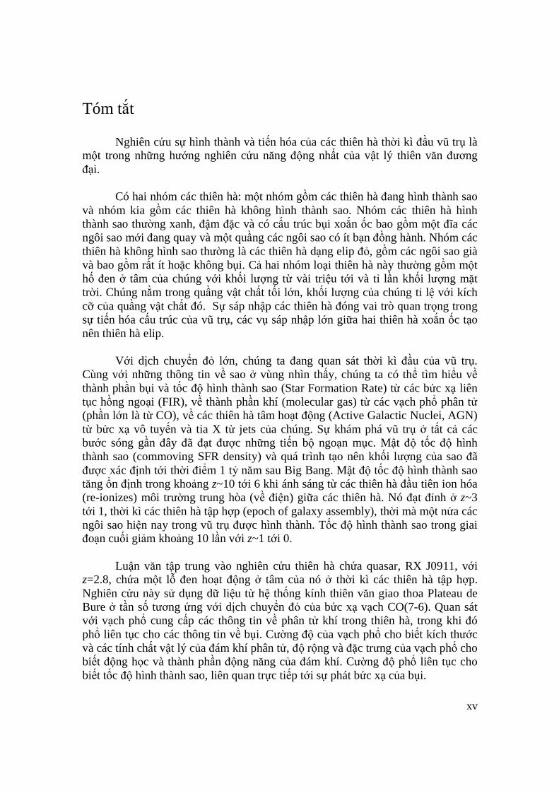
Tóm tắt Nghiên cứu sự hình thành và tiến hóa của các thiên hà thời kì đầu vũ trụ là một trong những hướng nghiên cứu năng động nhất của vật lý thiên văn đương đại.

Có hai nhóm các thiên hà: một nhóm gồm các thiên hà đang hình thành sao và nhóm kia gồm các thiên hà không hình thành sao. Nhóm các thiên hà hình thành sao thường xanh, đậm đặc và có cấu trúc bụi xoắn ốc bao gồm một đĩa các ngôi sao mới đang quay và một quầng các ngôi sao có ít bạn đồng hành. Nhóm các thiên hà không hình sao thường là các thiên hà dạng elip đỏ, gồm các ngôi sao già và bao gồm rất ít hoặc không bụi. Cả hai nhóm loại thiên hà này thường gồm một hố đen ở tâm của chúng với khối lượng từ vài triệu tới và tỉ lần khối lượng mặt trời. Chúng nằm trong quầng vật chất tối lớn, khối lượng của chúng tỉ lệ với kích cỡ của quầng vật chất đó. Sự sáp nhập các thiên hà đóng vai trò quan trọng trong sự tiến hóa cấu trúc của vũ trụ, các vụ sáp nhập lớn giữa hai thiên hà xoắn ốc tạo nên thiên hà elip.

Với dịch chuyển đỏ lớn, chúng ta đang quan sát thời kì đầu của vũ trụ.

Cùng với những thông tin về sao ở vùng nhìn thấy, chúng ta có thể tìm hiểu về thành phần bụi và tốc độ hình thành sao (Star Formation Rate) từ các bức xạ liên tục hồng ngoại (FIR), về thành phần khí (molecular gas) từ các vạch phổ phân tử (phần lớn là từ CO), về các thiên hà tâm hoạt động (Active Galactic Nuclei, AGN) từ bức xạ vô tuyến và tia X từ jets của chúng. Sự khám phá vũ trụ ở tất cả các bước sóng gần đây đã đạt được những tiến bộ ngoạn mục. Mật độ tốc độ hình thành sao (commoving SFR density) và quá trình tạo nên khối lượng của sao đã được xác định tới thời điểm 1 tỷ năm sau Big Bang. Mật độ tốc độ hình thành sao tăng ổn định trong khoảng z~10 tới 6 khi ánh sáng từ các thiên hà đầu tiên ion hóa (re-ionizes) môi trường trung hòa (về điện) giữa các thiên hà. Nó đạt đỉnh ở z~3 tới 1, thời kì các thiên hà tập hợp (epoch of galaxy assembly), thời mà một nửa các ngôi sao hiện nay trong vũ trụ được hình thành. Tốc độ hình thành sao trong giai đoạn cuối giảm khoảng 10 lần với z~1 tới 0.

Luận văn tập trung vào nghiên cứu thiên hà chứa quasar, RX J0911, với

z=2.8, chứa một lỗ đen hoạt động ở tâm của nó ở thời kì các thiên hà tập hợp. Nghiên cứu này sử dụng dữ liệu từ hệ thống kính thiên văn giao thoa Plateau de Bure ở tần số tương ứng với dịch chuyển đỏ của bức xạ vạch CO(7-6). Quan sát với vạch phổ cung cấp các thông tin về phân tử khí trong thiên hà, trong khi đó phổ liên tục cho các thông tin về bụi. Cường độ của vạch phổ cho biết kích thước và các tính chất vật lý của đám khí phân tử, độ rộng và đặc trưng của vạch phổ cho biết động học và thành phần động năng của đám khí. Cường độ phổ liên tục cho biết tốc độ hình thành sao, liên quan trực tiếp tới sự phát bức xạ của bụi.

xvi

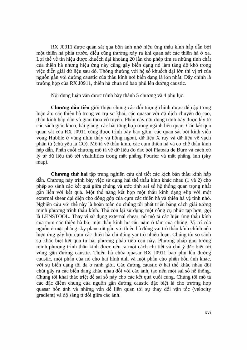
RX J0911 được quan sát qua bốn ảnh nhờ hiệu ứng thấu kính hấp dẫn bởi một thiên hà phía trước, điều cũng thường xảy ra khi quan sát các thiên hà ở xa. Lợi thế về tín hiệu được khuếch đại khoảng 20 lần cho phép tìm ra những tính chất của thiên hà nhưng hiệu ứng này cũng gây biến dạng nó làm tăng độ khó trong việc diễn giải dữ liệu sau đó. Thông thường với hệ số khuếch đại lớn thì vị trí của nguồn gần với đường caustic của thấu kính nơi biến dạng là lớn nhất. Đây chính là trường hợp của RX J0911, thiên hà chứa nó bao phủ lên đường caustic.

Nội dung luận văn được trình bày thành 5 chương và 4 phụ lục. Chương đầu tiên giới thiệu chung các đối tượng chính được đề cập trong

luận án: các thiên hà trong vũ trụ sơ khai, các quasar với độ dịch chuyển đỏ cao, thấu kính hấp dẫn và giao thoa vô tuyến. Phần này nội dung trình bày được lấy từ các sách giáo khoa, bài giảng, các bài tổng hợp trong ngành liên quan. Các kết quả quan sát của RX J0911 cũng được trình bày bao gồm: các quan sát bởi kính viễn vọng Hubble ở vùng nhìn thấy và hồng ngoại, dữ liệu X ray và dữ liệu về vạch phân tử (chủ yếu là CO). Mô tả về thấu kính, các cụm thiên hà và cơ chế thấu kính hấp dẫn. Phần cuối chương mô tả về dữ liệu đo đạc bởi Plateau de Bure và cách xử lý từ dữ liệu thô tới visibilities trong mặt phẳng Fourier và mặt phẳng ảnh (sky map).

Chương thứ hai tập trung nghiên cứu chi tiết các kịch bản thấu kính hấp

dẫn. Chương này trình bày việc sử dụng hai thế thấu kính khác nhau (1 và 2) cho phép so sánh các kết quả giữa chúng và ước tính sai số hệ thống quan trọng nhất gắn liền với kết quả. Một thế năng kết hợp một thấu kính dạng elip với một external shear đại diện cho đóng góp của cụm các thiên hà và thiên hà vệ tinh nhỏ. Nghiên cứu với thế này là hoàn toàn do chúng tôi phát triển bằng cách giải tường minh phương trình thấu kính. Thế còn lại sử dụng một công cụ phức tạp hơn, gọi là LENSTOOL. Thay vì sử dụng external shear, nó mô tả các hiệu ứng thấu kính của cụm các thiên hà bởi một thấu kính hư cấu nằm ở tâm của chúng. Vị trí của nguồn ở mặt phẳng sky plane rất gần với thiên hà đóng vai trò thấu kính chính nên hiệu ứng gây bởi cụm các thiên hà chỉ đóng vai trò nhiễu loạn. Chúng tôi so sánh sự khác biệt kết quả từ hai phương pháp tiếp cận này. Phương pháp giải tường minh phương trình thấu kính được nêu ra một cách chi tiết và chú ý đặc biệt tới vùng gần đường caustic. Thiên hà chứa quasar RX J0911 bao phủ lên đường caustic, một phần của nó cho hai hình ảnh và một phần cho phần bốn ảnh khác, với sự biến dạng tối đa ở ranh giới. Các đường caustic ở hai thế khác nhau đôi chút gây ra các biến dạng khác nhau đối với các ảnh, tạo nên một sai số hệ thống. Chúng tôi khai thác triệt để sai số này cho các kết quả cuối cùng. Chúng tôi mô tả các đặc điểm chung của nguồn gần đường caustic đặc biệt là cho trường hợp quasar bốn ảnh và những vấn đề liên quan tới sự thay đổi vận tốc (velocity gradient) và độ sáng tỉ đối giữa các ảnh.

xvii

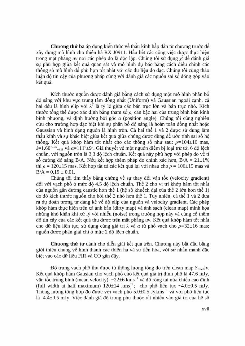
Chương thứ ba áp dụng kiến thức về thấu kính hấp dẫn từ chương trước để xây dựng mô hình cho thiên hà RX J0911. Hầu hết các công việc được thực hiện trong mặt phẳng uv nơi các phép đo là độc lập. Chúng tôi sử dụng χ2 để đánh giá sự phù hợp giữa kết quả quan sát và mô hình dự báo bằng cách điều chỉnh các thông số mô hình để phù hợp tốt nhất với các dữ liệu đo đạc. Chúng tôi cũng thảo luận độ tin cậy của phương pháp cùng với đánh giá các nguồn sai số đóng góp vào kết quả.

Kích thước nguồn được đánh giá bằng cách sử dụng một mô hình phân bố

độ sáng với khu vực trung tâm đồng nhất (Uniform) và Gaussian ngoài cạnh, cả hai đều là hình elip với λ2 là tỷ lệ giữa các bán trục lớn và bán trục nhỏ. Kích thước tổng thể được xác định bằng tham số ρ, căn bậc hai của trung bình bán kính bình phương, và định hướng bởi góc α (position angle). Chúng tôi cũng nghiên cứu cho trường hợp đặc biệt khi sự phân bố độ sáng là hoàn toàn đồng nhất hoặc Gaussian và hình dạng nguồn là hình tròn. Cả hai thế 1 và 2 được sử dụng làm thấu kính và sự khác biệt giữa kết quả giữa chúng được dùng để ước tính sai số hệ thống. Kết quả khớp hàm tốt nhất cho các thông số như sau: ρ=104±16 mas, λ=1.60+0.35

−0.18 và α=111o±9o. Giả thuyết về một nguồn điểm bị loại trừ tới 6 độ lệch chuẩn, với nguồn tròn là 3,3 độ lệch chuẩn. Kết quả này phù hợp với phép đo về tỉ số cường độ sáng B/A. Nếu kết hợp thêm phép đo chính xác hơn, B/A = 21±1% thì ρ = 120±15 mas. Kết hợp tất cả các kết quả lại với nhau cho ρ = 106±15 mas và B/A = 0.19 ± 0.01.

Chúng tôi tìm thấy bằng chứng về sự thay đổi vận tốc (velocity gradient) đối với vạch phổ ở mức độ 4.5 độ lệch chuẩn. Thế 2 cho vị trí khớp hàm tốt nhất của nguồn gần đường caustic hơn thế 1 (hệ số khuếch đại của thế 2 lớn hơn thế 1) do đó kích thước nguồn cho bởi thế 2 nhỏ hơn thế 1. Tuy nhiên, cả thế 1 và 2 đưa ra dự đoán tương tự đáng kể về độ elip của nguồn và velocity gradient. Các phép khớp hàm thực hiện trên cả ảnh bẩn (dirty map) và ảnh sạch (clean map) minh họa những khó khăn khi xử lý với nhiễu (noise) trong trường hợp này và củng cố thêm độ tin cậy của các kết quả thu được trên mặt phẳng uv. Kết quả khớp hàm tốt nhất cho dữ liệu liên tục, sử dụng cùng giá trị λ và α từ phổ vạch cho ρ=32±16 mas; nguồn được phân giải chỉ ở mức 2 độ lệch chuẩn. Chương thứ tư dành cho diễn giải kết quả trên. Chương này bắt đầu bằng giới thiệu chung về hình thành các thiên hà và sự tiến hóa, với sự nhấn mạnh đặc biệt vào các dữ liệu FIR và CO gần đây.

Độ trưng vạch phổ thu được từ thông lượng tổng đo trên clean map Sline∆ν. Kết quả khớp hàm Gausian cho vạch phổ cho kết quả giá trị đỉnh phổ là 47.6 mJy, vận tốc trung bình (mean velocity) −22±6 kms−1 và độ rộng tại nửa chiều cao đỉnh (full width at half maximum) 120±14 kms−1; cho phổ liên tục ~4.0±0.5 mJy. Thông lượng tổng hợp đo được với vạch phổ 5.0±0.5 Jykms−1 và với phổ liên tục là 4.4±0.5 mJy. Việc đánh giá độ trưng phụ thuộc rất nhiều vào giá trị của hệ số

xviii

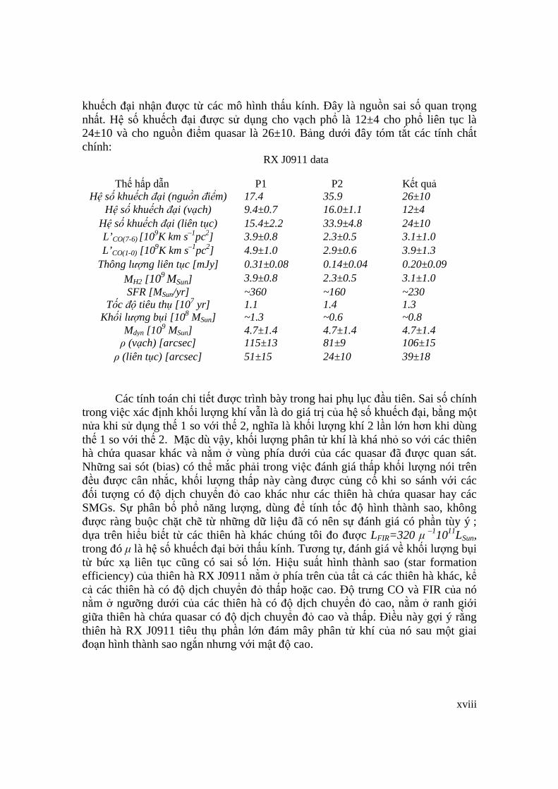
khuếch đại nhận được từ các mô hình thấu kính. Đây là nguồn sai số quan trọng nhất. Hệ số khuếch đại được sử dụng cho vạch phổ là 12±4 cho phổ liên tục là 24±10 và cho nguồn điểm quasar là 26±10. Bảng dưới đây tóm tắt các tính chất chính:

RX J0911 data Thế hấp dẫn P1 P2 Kết quả

Hệ số khuếch đại (nguồn điểm) 17.4 35.9 26±10 Hệ số khuếch đại (vạch) 9.4±0.7 16.0±1.1 12±4

Hệ số khuếch đại (liên tục) 15.4±2.2 33.9±4.8 24±10 L’CO(7-6) [109K km s–1pc2] 3.9±0.8 2.3±0.5 3.1±1.0 L’CO(1-0) [109K km s–1pc2] 4.9±1.0 2.9±0.6 3.9±1.3

Thông lượng liên tục [mJy] 0.31±0.08 0.14±0.04 0.20±0.09 MH2 [109 MSun] 3.9±0.8 2.3±0.5 3.1±1.0 SFR [MSun/yr] ~360 ~160 ~230

Tốc độ tiêu thụ [107 yr] 1.1 1.4 1.3 Khối lượng bụi [108 MSun] ~1.3 ~0.6 ~0.8

Mdyn [109 MSun] 4.7±1.4 4.7±1.4 4.7±1.4 ρ (vạch) [arcsec] 115±13 81±9 106±15

ρ (liên tục) [arcsec] 51±15 24±10 39±18 Các tính toán chi tiết được trình bày trong hai phụ lục đầu tiên. Sai số chính

trong việc xác định khối lượng khí vẫn là do giá trị của hệ số khuếch đại, bằng một nửa khi sử dụng thế 1 so với thế 2, nghĩa là khối lượng khí 2 lần lớn hơn khi dùng thế 1 so với thế 2. Mặc dù vậy, khối lượng phân tử khí là khá nhỏ so với các thiên hà chứa quasar khác và nằm ở vùng phía dưới của các quasar đã được quan sát. Những sai sót (bias) có thể mắc phải trong việc đánh giá thấp khối lượng nói trên đều được cân nhắc, khối lượng thấp này càng được củng cố khi so sánh với các đối tượng có độ dịch chuyển đỏ cao khác như các thiên hà chứa quasar hay các SMGs. Sự phân bố phổ năng lượng, dùng để tính tốc độ hình thành sao, không được ràng buộc chặt chẽ từ những dữ liệu đã có nên sự đánh giá có phần tùy ý ; dựa trên hiểu biết từ các thiên hà khác chúng tôi đo được LFIR=320 µ –11011LSun, trong đó µ là hệ số khuếch đại bởi thấu kính. Tương tự, đánh giá về khối lượng bụi từ bức xạ liên tục cũng có sai số lớn. Hiệu suất hình thành sao (star formation efficiency) của thiên hà RX J0911 nằm ở phía trên của tất cả các thiên hà khác, kể cả các thiên hà có độ dịch chuyển đỏ thấp hoặc cao. Độ trưng CO và FIR của nó nằm ở ngưỡng dưới của các thiên hà có độ dịch chuyển đỏ cao, nằm ở ranh giới giữa thiên hà chứa quasar có độ dịch chuyển đỏ cao và thấp. Điều này gợi ý rằng thiên hà RX J0911 tiêu thụ phần lớn đám mây phân tử khí của nó sau một giai đoạn hình thành sao ngắn nhưng với mật độ cao.

xix

So với các thiên hà chứa quasar khác, RX J0911 có độ rộng vạch phổ nhỏ đáng chú ý. Như vậy có thể đám mây phân tử khí nằm trong một cái đĩa đang quay có trục quay trùng với hướng nhìn. Tuy nhiên điều này lại mâu thuẫn với tính chất elip của nguồn đã đo được, do đó cần phải đánh giá cẩn trọng hơn về sai số của phép đo. Sử dụng kết quả đo độ trưng X-ray của RX J0911 bởi Fan và cộng sự năm 2009 chúng tôi nhận được bằng chứng củng cố thêm về khối lượng động học (dynamical mas) của nó nhỏ bất thường. Khi cả khối lượng đám mây khí và khối lượng động học nhỏ so với các thiên hà chứa quasar khác thì vấn đề không chỉ nằm ở khối lượng của hố đen ở tâm thiên hà này nhỏ.

Chương cuối tóm tắt lại nội dung công việc đã thực hiện và nêu lên hướng

nghiên cứu sau đó. Nghiên cứu chi tiết về một thiên hà chứa quasar ở xa ở vùng bước sóng mm

đã minh họa một số thuộc tính đáng chú ý nhất của các thiên hà ở xa và sự tiến hóa của chúng trong vũ trụ sơ khai khi hầu hết các ngôi sao hiện nay được hình thành. Nhờ hiệu ứng thấu kính hấp dẫn đã khuếch đại tín hiệu, độ nhạy và độ phân giải cao của hệ thống kính giao thoa Plateau de Bure đã quan sát được bức xạ vạch phổ CO và phổ liên tục để từ đó có thể phân giải được kích thước nguồn phát.

Nghiên cứu tỉ mỉ các tính chất của thấu kính hấp dẫn cho nguồn gần đường

caustic đã làm sáng tỏ tính chất đáng chú ý nhất của nó và có thể áp dụng cho các quan sát sau này của các thiên hà trong các tình huống tương tự. Xử lý dữ liệu ở đây đã minh họa những phức tạp của vấn đề và đánh giá được các nguồn sai số, đặc biệt là sự phụ thuộc mạnh của hệ số khuếch đại vào kích thước của nguồn.

Vạch phổ CO(7-6) được phân biệt rõ ràng trên một nền phổ liên tục nên có

thể tin cậy các phép đo độ trưng liên quan tới đám mây phân tử khí và bụi. Nghiên cứu đã chỉ ra có thể phân giải được nguồn phát và hình thái của nó như kích thước, độ elip, góc định hướng, và cung cấp bằng chứng về velocity gradient. Độ rộng vạch phổ CO(7-6) rất hẹp gợi ý khối lượng động học đám mây nhỏ phù hợp với khối lượng đám mây khí và bụi được xác định một cách độc lập. Hiệu suất hình thành sao lớn ngụ ý rằng thiên hà này đã tiêu thụ phần lớn đám mây khí trong một giai đoạn hình thành sao ngắn nhưng có cường độ lớn; nó nằm ở ranh giới giữa các thiên hà chứa quasar có độ dịch chuyển đỏ cao và thấp.

Đài thiên văn ALMA còn có độ nhạy và độ phân giải cao hơn so với

Plateau de Bure nên chúng tôi đề xuất quan sát một thiên hà chứa quasar tương tự như thiên hà RX J0911. Nó có 6 ảnh gây bởi hiệu ứng thấu kính hấp dẫn với hệ số khuếch đại khoảng 100. Như được trình bày trong phụ lục 3 và 4, chúng tôi có thể đạt tới độ phân giải cỡ 50 pc chỉ với 2 giờ quan sát ở vạch CO(9-8). Chúng tôi cũng chỉ ra khả năng có thể phát hiện một vạch phổ của phân tử nước cung cấp các thông tin hữu ích về độ trưng vùng hồng ngoại FIR.

xx

Những quan sát về các thiên hà chứa quasar ở xa chắc chắn rất triển vọng

và sẽ có đóng góp to lớn trong việc tìm hiểu cơ chế sự hình thành và tiến hóa của các cấu trúc thời kì vũ trụ sơ khai. Chúng tôi hy vọng có thể tham gia vào hành trình khám phá này dựa trên những kinh nghiệm thu được từ việc nghiên cứu thiên hà RX J0911.

xxi

TABLE OF CONTENT

1.1 Generalities ............................................................................................. 1

1.1.1 Galaxies in the early universe ................................................... 1

1.1.2 Quasars at high redshifts ........................................................... 3

1.1.3 Gravitational lensing ................................................................. 7

1.1.4 Radio interferometry ............................................................... 12

1.2 RX J0911: early observations ............................................................... 15

1.2.1 Quasar first observations ........................................................ 15

1.2.2 HST images, strong lensing and the cluster lens .................... 18

1.2.3 X-ray data and time delay ....................................................... 21

1.2.4 CO and other molecular data .................................................. 22

1.3 RX J0911: PdBI observations in CO(7-6) ............................................ 25

1.3.1 Antenna configuration and data taking conditions ................. 25

1.3.2 Calibration and noise .............................................................. 25

1.3.3 Mapping and deconvolution ................................................... 29

2.1 Introduction ........................................................................................... 34

2.2 Strong lensing: a reminder .................................................................... 34

2.2.1 General formalism .................................................................. 34

2.2.2 Extended sources .................................................................... 35

2.3 Solving the lens equation: a simple example ........................................ 39

2.4 Vicinity of the caustic and critical curve .............................................. 51

2.5 QSO RX J0911: lensing the point source ............................................. 53

2.5.1 Introduction ............................................................................. 53

2.5.2 Solving the lens equation using potential 1 ............................ 54

2.5.3 Solving the lens equation using potential 2 ............................ 58

2.6 QSO RX J0911: lensing the extended source ....................................... 59

2.6.1 Using potential 1 ..................................................................... 59

2.6.2 Using potential 2 ..................................................................... 61

2.6.3 Comparing the lensing properties of potentials 1 and 2 ......... 64

2.6.4 Comments on the relative merits of potentials 1 and 2 .......... 68

2.7 Additional comments ............................................................................ 69

2.7.1 B/A brightness ratio ................................................................ 69

Acknowledgements .................................................................................................. ii

Abstract ................................................................................................................... iii

Résumé .................................................................................................................... ix

Tóm tắt ................................................................................................................... xv

List of Figures ..................................................................................................... xxiii

List of Tables ...................................................................................................... xxvi

List of Abbreviations ......................................................................................... xxvii

1. Introduction .......................................................................................................... 1

2. Gravitational lensing of QSO RX J0911 ........................................................... 34

xxii

2.7.2 General case of quadruply imaged quasars ............................ 70

2.7.3 Velocity gradient..................................................................... 72

2.8 Summary and conclusion ...................................................................... 73

3.1 Introduction ........................................................................................... 74

3.2 Astrometry ............................................................................................ 74

3.3 Effects contributing to χ2 ...................................................................... 76

3.4 Source size ............................................................................................ 81

3.5 Source ellipticity ................................................................................... 84

3.6 B/A brightness ratio .............................................................................. 89

3.7 Velocity gradient ................................................................................... 90

3.8 Continuum ............................................................................................. 92

3.9 Fitting the clean map ............................................................................. 93

3.10 Fitting the dirty map............................................................................ 96

3.11 Summary and conclusion .................................................................... 99

4.1 Galaxy formation and evolution: an introduction ............................... 100

4.1.1 Generalities ........................................................................... 100

4.1.2 Recent Far Infrared (FIR) data from distant galaxies ........... 105

4.1.3 Recent CO data from distant galaxies .................................. 108

4.2 RX J0911: line luminosity .................................................................. 110

4.3 RX J0911: dust luminosity ................................................................. 115

4.4 RX J0911: line width .......................................................................... 117

A1. Line emission ..................................................................................... 129

A2. Dust emission ..................................................................................... 131

A3. Selection of a candidate for new observations: basic material .......... 135

A4. Proposal for observation at ALMA .................................................... 141

3. Modelling the host galaxy of QSO RX J0911 ................................................... 74

4. Interpretation of the results .............................................................................. 100

5. Summary and perspectives .............................................................................. 121

References ............................................................................................................ 123

Appendices ........................................................................................................... 129

List of Publications .............................................................................................. 147

xxiii

List of Figures

Figure 1.1 A typical low z molecular spectrum .................................................................. 2

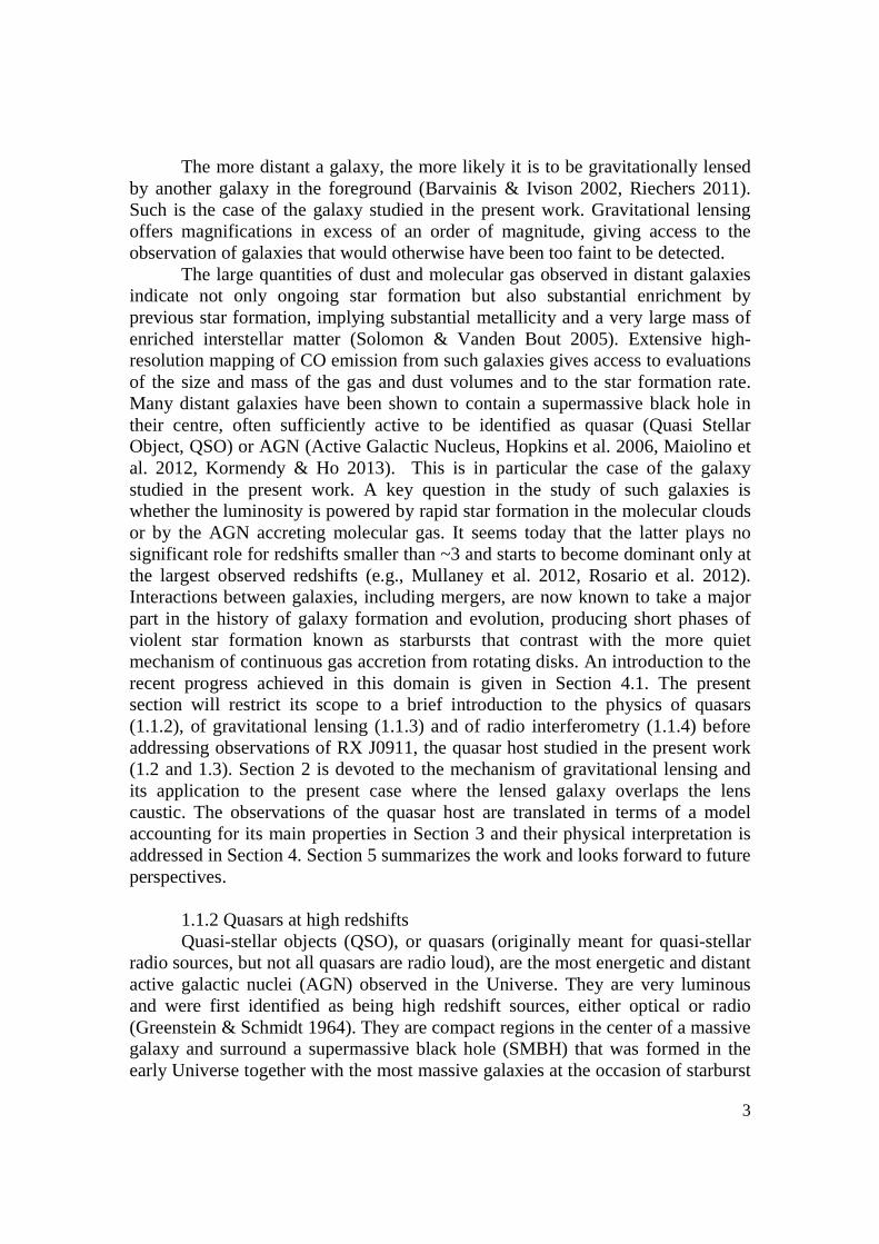
Figure 1.2. Schematic of an active galactic nucleus & VLA radio image of Cyg A .......... 4

Figure 1.3 HST image of the nearby quasar 3C 273........................................................... 5

Figure 1.4 X-ray image of PKS 1127-145 & Infrared image of a quasar-starburst pair ... 5

Figure 1.5 Abell 2218 Cluster ............................................................................................. 8

Figure 1.6 Image of the Bullet Cluster from the Hubble Space Telescope. ....................... 9

Figure 1.7 Einstein rings in several cases & a collection of Einstein rings ...................... 10

Figure 1.8 Examples of multiple images. ......................................................................... 10

Figure 1.9 Typical quadruply imaged quasars. ................................................................. 11

Figure 1.10 Image configuration in the case of QSO RX J0911. ..................................... 11

Figure 1.11 Plateau de Bure Interferometer ...................................................................... 12

Figure 1.12 Schematics of the signals on-line treatment from a pair of antennas ............ 14

Figure 1.13 High resolution images of RX J0911 ............................................................ 16

Figure 1.14 First evidence for the nearby lens cluster given by Burud et al. (1998).. ...... 17

Figure 1.15a The RX J0911 lensing cluster as studied by Kneib et al. (2000) ................ 19 Figure 1.15b The RX J0911 lensing morphology used by Kneib et al. (2000) ................ 19 Figure 1.16 CASTLES consortium HST images of RX J0911 ........................................ 20

Figure 1.17 Time dependence of X-ray fluxes& combined light curve of RX J0911 ....... 21

Figure 1.18 RX J0911 image from EVLA & the CO(1-0) line ........................................ 22

Figure 1.19 PdBI map of RX J0911 & 3.6 GHz spectrum of image A ............................ 23

Figure 1.20 Comparison of the CO(7-6) & CI(2-1) .......................................................... 23

Figure 1.21 Modelled SEDs for RX J0911. ...................................................................... 24

Figure 1.22 (u,v) coverage for the RX J0911 data collection. .......................................... 26

Figure 1.23 Amplitude calibration of one of the 15 baselines .......................................... 27

Figure 1.24 Phase calibration for one of the 15 baselines. ............................................... 27

Figure 1.25 RF passband calibration of one of the 15 baselines ...................................... 28

Figure 1.26 Calibrated visibilities in the complex plane .................................................. 28

Figure 1.27 Visibility amplitude versus (u,v) radius and (u,v) azimuth ........................... 29

Figure 1.28 Dirty beams . ................................................................................................. 30

Figure 1.29 Dirty maps for three different weightings. .................................................... 31

Figure 1.30 Clean maps and residuals for two different stopping parameters .................. 32

Figure 1.31 Clean maps for different weightings and different frequency intervals. ....... 33

Figure 2.1 Schematic geometry, coordinates definition & isotropic potential imaging ... 36

Figure 2.2 Dependence of the image positions & morphology on the source position .... 37

Figure 2.3 Image appearances for the same potential & source size as in Figure 2.2 ...... 38

Figure 2.4 Critical curve (black) and caustic (red) for γ0=0.25 and r0=1. ........................ 40

Figure 2.5 Dependence of f (γ0=0.25 & r0=1) & r1, r2, r3, r4 (rs=0.2) on φ ..................... 42

Figure 2.6 Dependence of f (γ0=0.25 & r0=1) & r1, r2, r3, r4 (rs=0.4) on φ ..................... 43

Figure 2.7 Same as Figures 2.5 & 2.6 (rs=0.2808), zoomed on the transition region ..... 44

Figure 2.8 Dependence on φ of r1, r2, M1, M2 for rs=0.2 .................................................. 45

Figure 2.9 Dependence on φ of r3, r4, M3, M4 for rs=0.2. ................................................. 46

Figure 2.10 Dependence on φ of r1, r2, M1, M2 for rs=0.4. ............................................... 47

Figure 2.11 Dependence on φ of r3, r4, M3, M4 for rs=0.4. ............................................... 48

xxiv

Figure 2.12 Dependence on φ of r1, r2, M1, M2 for rs=0.2808.. ........................................ 49

Figure 2.13 Dependence on φ of r3, r4, M3, M4 for rs=0.2808 ......................................... 50

Figure 2.14 Magnification of images close to the caustic as a function of rs & φ ............ 52

Figure 2.15 Source scan of the line φs=15o in steps of 0.0005 r0 starting at 0.25 r0 ........ 52

Figure 2.16 Values of gi & gi+1 whenever gi has a different sign from gi+1 ..................... 55

Figure 2.17 Distributions of |r1−r 2| & |r3−r 4|. ................................................................... 55

Figure 2.18 Distribution of |r1−r 2| and of |r3−r 4| .............................................................. 56

Figure 2.19 Image positions using potential 1 & map of images for point sources ......... 57

Figure 2.20 The χ2 distribution of the match between the HST images & potential 1. .... 57

Figure 2.21 Positions of images close to the critical curve............................................... 60

Figure 2.22 Histograms of distances which images move in the cell-splitting process ... 60

Figure 2.23 Histograms of differences in magnifications in the cell-splitting process .... 61

Figure 2.24 Positions of images (using potential 1) close to the critical curve. ............... 61

Figure 2.25 Distribution of the number of images produced by LENSTOOL. ................ 62

Figure 2.26 Positions of sources (using LENSTOOL) producing either 3 or 5 images ... 62

Figure 2.27 Evolution of images obtained using LENSTOOL for a source scan ............. 63

Figure 2.28 Distribution of the positions adopted for the A images. ................................ 64

Figure 2.29 Source positions which two potentials have a different number of images .. 65

Figure 2.30 Distributions of the mean distance ∆xy and of the image magnifications ∆M 65

Figure 2.31 χ2 distributions to the HST images predicted by potential 1& 2 ................... 66

Figure 2.32 Distributions of the image magnifications (disk radius 200 mas). ................ 66

Figure 2.33 Image densities for various disk sources ....................................................... 67

Figure 2.34 Image brightness distributions in radius & in polar angle ............................. 67

Figure 2.35 Dependence of the B/A brightness ratio on the source radius....................... 68

Figure 2.36 Distribution of the magnifications for the three A images & image B ......... 70

Figure 2.37 Typical quadruply imaged quasars (Saha & Williams classification)........... 71

Figure 2.38 A images of a split source having Rs=0.15” ................................................. 72

Figure 3.1 Sky map of the χ2 distribution for a uniform disk using potential 1................ 75

Figure 3.2 RX J0911 data in term of visibility ................................................................. 78

Figure 3.3 Source map of χ2 using a common and constant weight (σ =0.1082).. ........... 79

Figure 3.4 Dependence on measurement number of the weights used by GILDAS ........ 80

Figure 3.5 Dependence of the GILDAS weight on measurement number.. ..................... 80

Figure 3.6 Distribution of the GILDAS weights. ............................................................. 81

Figure 3.7 χ2 distributions for the line & the continuum as a function of ρ (mas)............ 82

Figure 3.8 χ2 map in the (λ,α) parameter space using potential 1 ..................................... 84

Figure 3.9 Dependence of χ2 on λ for various values of α using both potentials .............. 85

Figure 3.10 χ2 maps in the (λ,α) parameter space for both potentials ............................... 86

Figure 3.11 Dependence of the A image appearance on the source ellipticity ................. 86

Figure 3.12 Dependence of the best-fit value of ρ as a function of λ at fixed α ............... 87 Figure 3.13 Dependence of ρ on λ and α for both potentials. ........................................... 87

Figure 3.14 Dependence of χ2 on λ for fixed α and for both potentials. ........................... 88

Figure 3.15 Maps of the best-fit sources for both potentials. ........................................... 88

Figure 3.16 Dependence of the B/A ratio on ρ ................................................................. 89

Figure 3.17 Results of the best-fit velocity gradient for both potentials. ......................... 91

Figure 3.18 Sky maps of the two half parts of the line & of the source. .......................... 92

Figure 3.19 Continuum: dependence of the best-fit χ2 on the source size ρ ..................... 92

xxv

Figure 3.20 Distribution of the difference between original & reconstructed pixels ....... 94

Figure 3.21 Sky map of the difference.............................................................................. 94

Figure 3.22 Projections on x (upper panels) and y (lower panels) of the difference ........ 95

Figure 3.23 Dependence on ρ of the value of χ2 ............................................................... 95

Figure 3.24 Clean maps of the differences: noisy & noise-less models; model & data ... 96

Figure 3.25 Dirty map of the difference: original & reconstructed pixel contents ........... 97

Figure 3.26 Projections on x (upper panels) and y (lower panels) of the difference ........ 97

Figure 3.27 Dependence on ρ of the value of χ2.. ............................................................. 98

Figure 3.28 Dirty maps of the differences: noisy & noise-less models; model & data .... 99

Figure 4.1 A spiral, ESO 510-G13, warped by a collision with another galaxy ............ 101

Figure 4.2 M-σ relation ................................................................................................... 101

Figure 4.3 A typical result from a simulation of structure formation ............................. 102

Figure 4.4 Spectral energy distributions for main sequence & starburst ........................ 102

Figure 4.5 CO emission ladder ....................................................................................... 103

Figure 4.6 z~10 galaxy discovered by the HST & SMGs recently detected by ALMA . 104

Figure 4.7 Discovery history of z>1 molecular line detections ...................................... 105

Figure 4.8 SFR vs. Mstars & IR8 for z~0........................................................................... 106

Figure 4.9 RSB vs. IR8, SFR-Mstars & sSFR vs ΣIR relation for z~0. ............................... 106

Figure 4.10 Stacked HST images of MS & SB galaxies for various z ranges .............. 107

Figure 4.11 Dependence of the CO line width on CO luminosity & FIR luminosity .... 108

Figure 4.12 Redshift dependence of the mass fraction of gas to stars. ........................... 109

Figure 4.13 Dependence of the FIR luminosity on the CO luminosity. ......................... 110

Figure 4.14 Flux spectrum summed over the A and B images ....................................... 111

Figure 4.15 Flux spectrum over the A images using various weightings ...................... 112

Figure 4.16 Molecular gas mass vs. CO line FWHM ..................................................... 114

Figure 4.17 Wavelength dependence of the measured dust luminosity of RX J0911. ... 115

Figure 4.18 Relation between FIR and CO line luminosities for various galaxies... ........ 117

Figure 4.19 Distribution of LFIR /L'CO , as a function of LFIR & redshift ......................... 118

Figure 4.20 The CO line width vs. CO line luminosity & vs.FIR luminosity ................ 118

Figure 4.21 Molecular gas mass vs. CO line & RX J0911. ............................................ 119

Figure 4.22 MBH-σ relation for SMGs (blue circles) in the Bothwell 2013 sample. ....... 120

xxvi

List of Tables Table 1.1 Flux ratios for all four QSO components, relative to A1.................................. 15

Table 1.2 Photometric and astrometric properties of RX J0911 and the lensing galaxy .. 16

Table 1.3 Parameters of the best fit potential ................................................................... 18

Table 1.4 Best fit image coordinates and magnifications ................................................. 18

Table 1.5 CASTLES position and flux data ..................................................................... 20

Table 1.6 Parameters used in the CLEAN algorithm. ...................................................... 32

Table 2.1 Case of a sphere+shear potential: useful expressions ....................................... 39

Table 2.2 Potential 1, some useful expressions. ............................................................... 54

Table 2.3 Best fit results (r in arcseconds and φ in degrees) ............................................ 56

Table 2.4 Best fit values of the parameters ....................................................................... 57

Table 2.5 Parameters of the LENSTOOL potentials ........................................................ 58

Table 2.6 Positions and magnifications of the point images ............................................ 58

Table 3.1 Astrometry results obtained on the line & continuum using potential 1 .......... 76

Table 3.2 Best fit results on the source size ...................................................................... 82

Table 3.3 Different evaluations of the systematic uncertainty on the source size ρ. ........ 83

Table 3.4 Best-fit values of ρ (mas) evaluated with different methods .......................... 98

Table 4.1 RX J0911 data ................................................................................................. 113

Table 4.2 Measured flux densities of RX J0911.4+0551 ............................................... 115

xxvii

List of Abbreviations General AGN Active Galactic Nucleus BH Black Hole CASTLE CfA-Arizona Space Telescope LEns Survey CMA Cold Mode Accretion CMB Cosmic Microwave Background CSG Colour Selected Galaxy DEC Declination ERO Extremely Red Object FFT Fast Fourier Transform FIR Far-Infrared FWHM Full Width at Half Maximum GMC Giant Molecular Cloud HERACLES HERA CO Line Extragalactic Survey IF Intermediate Frequency IGM Intergalactic Medium IR Infrared ISM Interstellar Medium ISRF Interstellar Radiation Field ΛCDM Lambda Cold Dark Matter LIRG Luminous Infrared Galaxy (LIR>1011Lsun) LBG Lyman-Break Galaxy MS Main Sequence PA Position Angle PSF Point Spread Function PAH Polycyclic Aromatic Hydrocarbon QSO Quasi-Stellar Object RA Right Ascension RF Radio Frequency RG Radio Galaxy RMS Root Mean Square SB Starburst SDSS Sloan Digital Sky Survey SED Spectral Energy Distributions SFR Star-Formation Rate SIS Single Isothermal Sphere SMBH Supermassive Black Hole SMG Submillimeter Galaxy sSFR Specific Star-Formation Rate

xxviii

THINGS The HI Nearby Galaxy Survey ULIRG Ultraluminous Infrared Galaxy (LIR>1012 Lsun) WHIM Warm–Hot Intergalactic Medium WVR Water Vapour Radiometer Telescopes, Instruments and sofwares 30m IRAM 30m Telescope ACS Advanced Camera for Surveys ALMA Atacama Large (sub-) Millimeter Array CARMA Combined Array for Research in Millimeter-wave

Astronomy CLIC Continuum and Line Interferometer Calibration EVLA Expanded Very Large Array GILDAS Grenoble Imaging and Line Data Analysis System GREG Grenoble Graphic HIRAC High Resolution Adaptive Camera HST Hubble Space Telescope NOT Nordic Optical Telescope NTT ESO 3.5 m New Technology Telescope PdBI Plateau de Bure Interferometer SKA Square Kilometre Array SPIRE Spectral and Photometric Imaging Receiver VLA Very Large Array VLT Very Large Telescope Institutes and Organizations CNRS Centre national de la recherche scientifique ESA European Space Agency ESO European Southern Observatory NASA National Aeronautics and Space Administration IRAM Institut de Radioastronomie Millimetrique STScI Space Telescope Science Institute

1

1. Introduction

The present work reports the analysis of observations of the host galaxy of a high-z quasar using the Plateau de Bure interferometer, the aim being to contribute new information to our knowledge and understanding of the early Universe. I have collected in this introduction material that puts the work in context and paves the way toward its easy presentation. It includes three different sections. A first section recalls basic general information of relevance that can be found in lectures, textbooks, encyclopedy articles and review articles of a very broad reach. The second section summarizes the information that was available on RX J0911 before the present observations were made; it helps the reader in understanding in which context the decision to collect new data had been taken and explains why this target had been chosen as a good candidate. The third section summarizes the observations that have been made and describes the steps that have been taken to reduce the raw data into visibilities and sky maps that are used as basic material in the rest of the thesis.

1.1 Generalities 1.1.1 Galaxies in the early universe Understanding how the Universe evolved from the epoch of recombination,

when ~0.4 Myr after the Big Bang electrons combined with hydrogen and helium nuclei to form atoms, is a major task of present days astrophysics. At that time, the Universe was nearly perfectly isotropic and contained, in addition to the newly formed atoms, large quantities of dark matter, ~5 times more in mass than atoms, probably made of an unknown species of massive particles having negligible interactions other than gravity. One of the many important recent advances in our knowledge of the distant, early Universe comes from observations of spectral line emission from interstellar molecular gas, the raw material from which stars form, in high-redshift galaxies. A recent article (Solomon & Vanden Bout 2005) reviews the present situation, which I summarize in the following lines. Such observations tell us about the location, mass and physical conditions of molecular clouds during the epoch of galaxy formation. At the same time, observations of the underlying continuum tell us about black body radiation from interstellar dust grains.

As helium does not exist as molecules but only as atoms, and as hydrogen molecules have no electric dipole moment, the direct detection of the main constituents of the early Universe does not offer sufficient sensitivity to explore it efficiently. On the contrary, CO molecules, while rarer, are easy to excite into rotational and vibrational modes and are excellent tracers of the early gaseous Universe. While carbon was not present at the time of recombination, but only appeared as the first stars started to die, we know now that less than a Gyr after the Big Bang it had already been produced in sufficient quantity to be detected down to redshifts as large as ~10 (Carilli & Walter 2013). Its detection in early distant

2

galaxies tells us about the mechanisms of galaxy and supermassive back hole formation, and about their evolution to present days.

Observation of emission from CO rotational transitions (J-J–1) is indeed the dominant means of tracing interstellar molecular clouds, which consist almost entirely of molecular hydrogen rather than atomic hydrogen when the particle density is in excess of 100 cm-3 (Flower & Launay1985, Yang et al. 2010). Molecular clouds are the raw material for star formation and a critical component in the evolution of galaxies. The first generation of stars must have formed, in the absence of heavy elements, from HI with only trace amounts of H2 available to provide essential cooling. However, the very large infrared (IR) luminosity seen in ultraluminous and luminous infrared galaxies (ULIRGs and LIRGs) is clearly emitted by interstellar dust, and one expects all dense, dusty clouds to be molecular (Frayer et al. 1998, Neri et al. 2003, Bothwell et al. 2010, 2013).

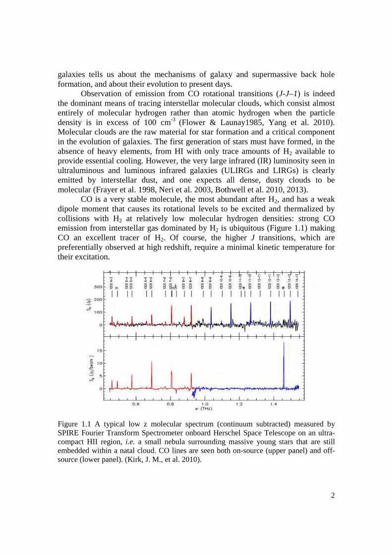
CO is a very stable molecule, the most abundant after H2, and has a weak dipole moment that causes its rotational levels to be excited and thermalized by collisions with H2 at relatively low molecular hydrogen densities: strong CO emission from interstellar gas dominated by H2 is ubiquitous (Figure 1.1) making CO an excellent tracer of H2. Of course, the higher J transitions, which are preferentially observed at high redshift, require a minimal kinetic temperature for their excitation.

Figure 1.1 A typical low z molecular spectrum (continuum subtracted) measured by SPIRE Fourier Transform Spectrometer onboard Herschel Space Telescope on an ultra-compact HII region, i.e. a small nebula surrounding massive young stars that are still embedded within a natal cloud. CO lines are seen both on-source (upper panel) and off-source (lower panel). (Kirk, J. M., et al. 2010).

3

The more distant a galaxy, the more likely it is to be gravitationally lensed by another galaxy in the foreground (Barvainis & Ivison 2002, Riechers 2011). Such is the case of the galaxy studied in the present work. Gravitational lensing offers magnifications in excess of an order of magnitude, giving access to the observation of galaxies that would otherwise have been too faint to be detected.

The large quantities of dust and molecular gas observed in distant galaxies indicate not only ongoing star formation but also substantial enrichment by previous star formation, implying substantial metallicity and a very large mass of enriched interstellar matter (Solomon & Vanden Bout 2005). Extensive high-resolution mapping of CO emission from such galaxies gives access to evaluations of the size and mass of the gas and dust volumes and to the star formation rate. Many distant galaxies have been shown to contain a supermassive black hole in their centre, often sufficiently active to be identified as quasar (Quasi Stellar Object, QSO) or AGN (Active Galactic Nucleus, Hopkins et al. 2006, Maiolino et al. 2012, Kormendy & Ho 2013). This is in particular the case of the galaxy studied in the present work. A key question in the study of such galaxies is whether the luminosity is powered by rapid star formation in the molecular clouds or by the AGN accreting molecular gas. It seems today that the latter plays no significant role for redshifts smaller than ~3 and starts to become dominant only at the largest observed redshifts (e.g., Mullaney et al. 2012, Rosario et al. 2012). Interactions between galaxies, including mergers, are now known to take a major part in the history of galaxy formation and evolution, producing short phases of violent star formation known as starbursts that contrast with the more quiet mechanism of continuous gas accretion from rotating disks. An introduction to the recent progress achieved in this domain is given in Section 4.1. The present section will restrict its scope to a brief introduction to the physics of quasars (1.1.2), of gravitational lensing (1.1.3) and of radio interferometry (1.1.4) before addressing observations of RX J0911, the quasar host studied in the present work (1.2 and 1.3). Section 2 is devoted to the mechanism of gravitational lensing and its application to the present case where the lensed galaxy overlaps the lens caustic. The observations of the quasar host are translated in terms of a model accounting for its main properties in Section 3 and their physical interpretation is addressed in Section 4. Section 5 summarizes the work and looks forward to future perspectives.

1.1.2 Quasars at high redshifts Quasi-stellar objects (QSO), or quasars (originally meant for quasi-stellar

radio sources, but not all quasars are radio loud), are the most energetic and distant active galactic nuclei (AGN) observed in the Universe. They are very luminous and were first identified as being high redshift sources, either optical or radio (Greenstein & Schmidt 1964). They are compact regions in the center of a massive galaxy and surround a supermassive black hole (SMBH) that was formed in the early Universe together with the most massive galaxies at the occasion of starburst

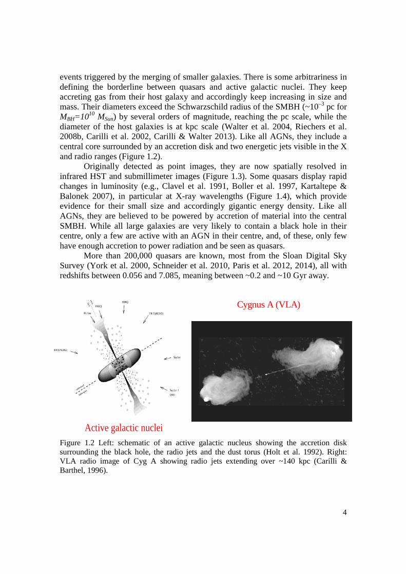
4

events triggered by the merging of smaller galaxies. There is some arbitrariness in defining the borderline between quasars and active galactic nuclei. They keep accreting gas from their host galaxy and accordingly keep increasing in size and mass. Their diameters exceed the Schwarzschild radius of the SMBH (~10–3 pc for MBH=1010 MSun) by several orders of magnitude, reaching the pc scale, while the diameter of the host galaxies is at kpc scale (Walter et al. 2004, Riechers et al. 2008b, Carilli et al. 2002, Carilli & Walter 2013). Like all AGNs, they include a central core surrounded by an accretion disk and two energetic jets visible in the X and radio ranges (Figure 1.2).

Originally detected as point images, they are now spatially resolved in infrared HST and submillimeter images (Figure 1.3). Some quasars display rapid changes in luminosity (e.g., Clavel et al. 1991, Boller et al. 1997, Kartaltepe & Balonek 2007), in particular at X-ray wavelengths (Figure 1.4), which provide evidence for their small size and accordingly gigantic energy density. Like all AGNs, they are believed to be powered by accretion of material into the central SMBH. While all large galaxies are very likely to contain a black hole in their centre, only a few are active with an AGN in their centre, and, of these, only few have enough accretion to power radiation and be seen as quasars.

More than 200,000 quasars are known, most from the Sloan Digital Sky Survey (York et al. 2000, Schneider et al. 2010, Paris et al. 2012, 2014), all with redshifts between 0.056 and 7.085, meaning between ~0.2 and ~10 Gyr away.

Figure 1.2 Left: schematic of an active galactic nucleus showing the accretion disk surrounding the black hole, the radio jets and the dust torus (Holt et al. 1992). Right: VLA radio image of Cyg A showing radio jets extending over ~140 kpc (Carilli & Barthel, 1996).

Active galactic nuclei

Cygnus A (VLA)

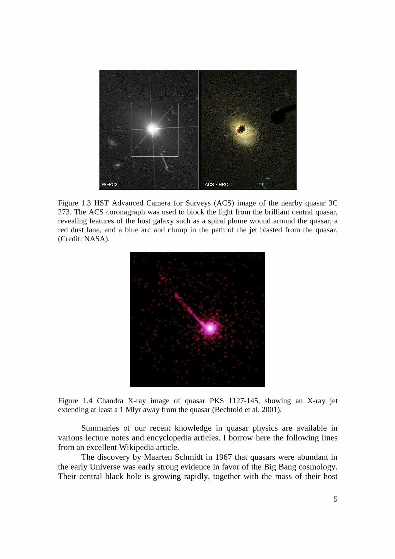
5

Figure 1.3 HST Advanced Camera for Surveys (ACS) image of the nearby quasar 3C 273. The ACS coronagraph was used to block the light from the brilliant central quasar, revealing features of the host galaxy such as a spiral plume wound around the quasar, a red dust lane, and a blue arc and clump in the path of the jet blasted from the quasar. (Credit: NASA).

Figure 1.4 Chandra X-ray image of quasar PKS 1127-145, showing an X-ray jet extending at least a 1 Mlyr away from the quasar (Bechtold et al. 2001).

Summaries of our recent knowledge in quasar physics are available in various lecture notes and encyclopedia articles. I borrow here the following lines from an excellent Wikipedia article.

The discovery by Maarten Schmidt in 1967 that quasars were abundant in the early Universe was early strong evidence in favor of the Big Bang cosmology. Their central black hole is growing rapidly, together with the mass of their host

6

galaxy; their jets, electromagnetic emission and winds slow down the formation of new stars, a process called 'feedback'. The jets that produce strong radio emission in some quasars at the centers of clusters of galaxies are known to have enough power to prevent the hot gas in those clusters from cooling and falling onto the central galaxy.

Quasars' luminosities are variable, with time scales that range from months to hours. This means that quasars generate and emit their energy from a very small region, since each part of the quasar would have to be in contact with other parts on such a time scale to allow the coordination of the luminosity variations. The emission of large amounts of power from a small region requires a power source far more efficient than the nuclear fusion that powers stars. The release of gravitational energy by matter falling towards a massive black hole is the only process known that can produce such high power continuously. Stellar explosions – supernovas and gamma-ray bursts – can do likewise, but only for a short while (from wiki). Quasars can be detected over the entire observable electromagnetic spectrum including radio, infrared, visible light, ultraviolet, X-ray and even gamma rays. Most quasars are brightest in their rest-frame near-ultraviolet wavelength of 121.6 nm (Lyman-alpha emission line of hydrogen), but due to the tremendous redshifts of these sources, the peak luminosity has been observed as far in the red as 900 nm, namely in the near infrared. A minority of quasars show strong radio emission, which originates from jets of matter moving close to the speed of light. When observed in the jet direction, these appear as blazars and often have regions that appear to (but do not) move away from the center faster than the speed of light (superluminal expansion).

Since quasars exhibit properties common to all active galaxies, the emission from quasars can be readily compared with those of smaller active galaxies powered by smaller supermassive black holes. To create a typical luminosity of 1040 watts, a super-massive black hole needs to consume ~10 MSun/yr, ~1000 MSun/yr for the brightest known quasars. The largest known is estimated to consume the equivalent of 600 Earths per minute. Quasar luminosities can vary considerably over time, depending on their surroundings. Since it is difficult to fuel quasars for many billions of years, after a quasar finishes accreting the surrounding gas and dust, it becomes an ordinary galaxy.

The oldest known quasars give evidence for the intergalactic medium (IGM) at that time being neutral gas. More recent quasars show no absorption region but rather their spectra contain a spiky area known as the Lyman-alpha forest, indicating that the IGM has undergone reionization into plasma, and that neutral gas exists only in small clouds.

Quasars show evidence of elements heavier than helium, indicating that galaxies underwent a massive phase of star formation shortly after the Big Bang.

Like all (unobscured) active galaxies, quasars can be strong X-ray sources. Radio-loud quasars can also produce X-rays and gamma rays by inverse Compton

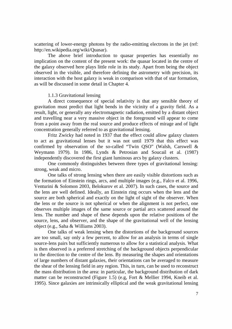
7

scattering of lower-energy photons by the radio-emitting electrons in the jet (ref: http://en.wikipedia.org/wiki/Quasar).

The above brief introduction to quasar properties has essentially no implication on the content of the present work: the quasar located in the centre of the galaxy observed here plays little role in its study. Apart from being the object observed in the visible, and therefore defining the astrometry with precision, its interaction with the host galaxy is weak in comparison with that of star formation, as will be discussed in some detail in Chapter 4.

1.1.3 Gravitational lensing A direct consequence of special relativity is that any sensible theory of

gravitation must predict that light bends in the vicinity of a gravity field. As a result, light, or generally any electromagnetic radiation, emitted by a distant object and travelling near a very massive object in the foreground will appear to come from a point away from the real source and produce effects of mirage and of light concentration generally referred to as gravitational lensing.

Fritz Zwicky had noted in 1937 that the effect could allow galaxy clusters to act as gravitational lenses but it was not until 1979 that this effect was confirmed by observation of the so-called “Twin QSO” (Walsh, Carswell & Weymann 1979). In 1986, Lynds & Petrosian and Soucail et al. (1987) independently discovered the first giant luminous arcs by galaxy clusters.

One commonly distinguishes between three types of gravitational lensing: strong, weak and micro.

One talks of strong lensing when there are easily visible distortions such as the formation of Einstein rings, arcs, and multiple images (e.g., Falco et al. 1996, Venturini & Solomon 2003, Belokurov et al. 2007). In such cases, the source and the lens are well defined. Ideally, an Einstein ring occurs when the lens and the source are both spherical and exactly on the light of sight of the observer. When the lens or the source is not spherical or when the alignment is not perfect, one observes multiple images of the same source or partial arcs scattered around the lens. The number and shape of these depends upon the relative positions of the source, lens, and observer, and the shape of the gravitational well of the lensing object (e.g., Saha & Williams 2003).

One talks of weak lensing when the distortions of the background sources are too small, say only a few percent, to allow for an analysis in terms of single source-lens pairs but sufficiently numerous to allow for a statistical analysis. What is then observed is a preferred stretching of the background objects perpendicular to the direction to the centre of the lens. By measuring the shapes and orientations of large numbers of distant galaxies, their orientations can be averaged to measure the shear of the lensing field in any region. This, in turn, can be used to reconstruct the mass distribution in the area: in particular, the background distribution of dark matter can be reconstructed (Figure 1.5) (e.g, Fort & Mellier 1994, Kneib et al. 1995). Since galaxies are intrinsically elliptical and the weak gravitational lensing

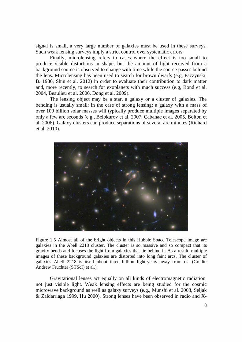
8

signal is small, a very large number of galaxies must be used in these surveys. Such weak lensing surveys imply a strict control over systematic errors.

Finally, microlensing refers to cases where the effect is too small to produce visible distortions in shape, but the amount of light received from a background source is observed to change with time while the source passes behind the lens. Microlensing has been used to search for brown dwarfs (e.g, Paczynski, B. 1986, Shin et al. 2012) in order to evaluate their contribution to dark matter and, more recently, to search for exoplanets with much success (e.g, Bond et al. 2004, Beaulieu et al. 2006, Dong et al. 2009).

The lensing object may be a star, a galaxy or a cluster of galaxies. The bending is usually small: in the case of strong lensing: a galaxy with a mass of over 100 billion solar masses will typically produce multiple images separated by only a few arc seconds (e.g., Belokurov et al. 2007, Cabanac et al. 2005, Bolton et al. 2006). Galaxy clusters can produce separations of several arc minutes (Richard et al. 2010).

Figure 1.5 Almost all of the bright objects in this Hubble Space Telescope image are galaxies in the Abell 2218 cluster. The cluster is so massive and so compact that its gravity bends and focuses the light from galaxies that lie behind it. As a result, multiple images of these background galaxies are distorted into long faint arcs. The cluster of galaxies Abell 2218 is itself about three billion light-years away from us. (Credit: Andrew Fruchter (STScI) et al.).

Gravitational lenses act equally on all kinds of electromagnetic radiation,

not just visible light. Weak lensing effects are being studied for the cosmic microwave background as well as galaxy surveys (e.g., Munshi et al. 2008, Seljak & Zaldarriaga 1999, Hu 2000). Strong lenses have been observed in radio and X-

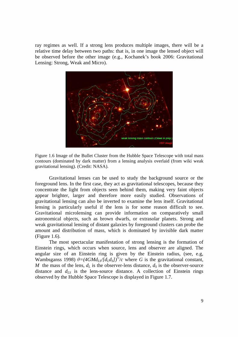
9

ray regimes as well. If a strong lens produces multiple images, there will be a relative time delay between two paths: that is, in one image the lensed object will be observed before the other image (e.g., Kochanek’s book 2006: Gravitational Lensing: Strong, Weak and Micro).

Figure 1.6 Image of the Bullet Cluster from the Hubble Space Telescope with total mass contours (dominated by dark matter) from a lensing analysis overlaid (from wiki weak gravitational lensing). (Credit: NASA).

Gravitational lenses can be used to study the background source or the

foreground lens. In the first case, they act as gravitational telescopes, because they concentrate the light from objects seen behind them, making very faint objects appear brighter, larger and therefore more easily studied. Observations of gravitational lensing can also be inverted to examine the lens itself. Gravitational lensing is particularly useful if the lens is for some reason difficult to see. Gravitational microlensing can provide information on comparatively small astronomical objects, such as brown dwarfs, or extrasolar planets. Strong and weak gravitational lensing of distant galaxies by foreground clusters can probe the amount and distribution of mass, which is dominated by invisible dark matter (Figure 1.6).

The most spectacular manifestation of strong lensing is the formation of Einstein rings, which occurs when source, lens and observer are aligned. The angular size of an Einstein ring is given by the Einstein radius, (see, e.g, Wambsganss 1998) θ=(4GMdLS/[dLdS])

½/c where G is the gravitational constant, M the mass of the lens, dL is the observer-lens distance, dS is the observer-source distance and dLS is the lens-source distance. A collection of Einstein rings observed by the Hubble Space Telescope is displayed in Figure 1.7.

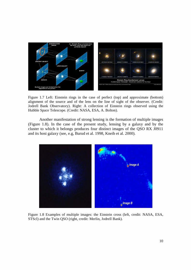
10

Figure 1.7 Left: Einstein rings in the case of perfect (top) and approximate (bottom) alignment of the source and of the lens on the line of sight of the observer. (Credit: Jodrell Bank Observatory). Right: A collection of Einstein rings observed using the Hubble Space Telescope. (Credit: NASA, ESA, A. Bolton).

Another manifestation of strong lensing is the formation of multiple images

(Figure 1.8). In the case of the present study, lensing by a galaxy and by the cluster to which it belongs produces four distinct images of the QSO RX J0911 and its host galaxy (see, e.g, Burud et al. 1998, Kneib et al. 2000).

Figure 1.8 Examples of multiple images: the Einstein cross (left, credit: NASA, ESA, STScl) and the Twin QSO (right, credit: Merlin, Jodrell Bank).

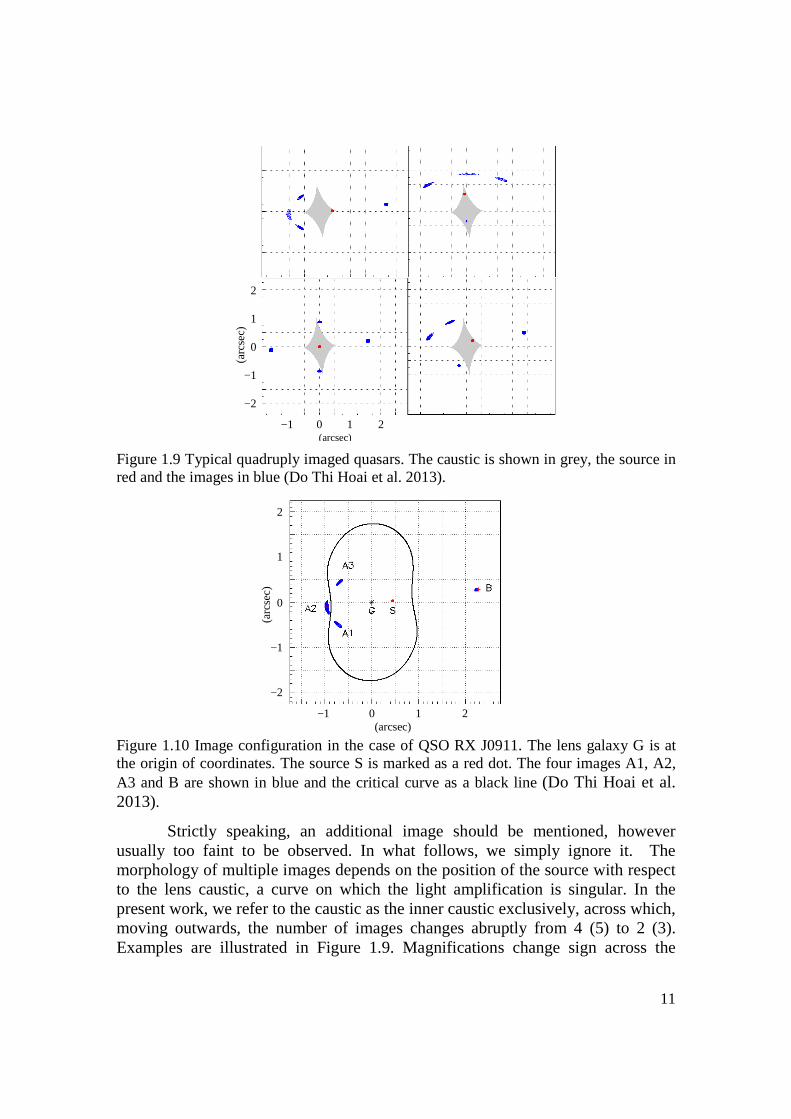
11

Figure 1.9 Typical quadruply imaged quasars. The caustic is shown in grey, the source in red and the images in blue (Do Thi Hoai et al. 2013).

Figure 1.10 Image configuration in the case of QSO RX J0911. The lens galaxy G is at the origin of coordinates. The source S is marked as a red dot. The four images A1, A2, A3 and B are shown in blue and the critical curve as a black line (Do Thi Hoai et al. 2013).

Strictly speaking, an additional image should be mentioned, however usually too faint to be observed. In what follows, we simply ignore it. The morphology of multiple images depends on the position of the source with respect to the lens caustic, a curve on which the light amplification is singular. In the present work, we refer to the caustic as the inner caustic exclusively, across which, moving outwards, the number of images changes abruptly from 4 (5) to 2 (3). Examples are illustrated in Figure 1.9. Magnifications change sign across the

2

1

0

−1

−2

(arc

sec)

(arcsec) −1 0 1 2

2

1

0

−1

−2

(arcsec)

(arc

sec)

−1 0 1 2

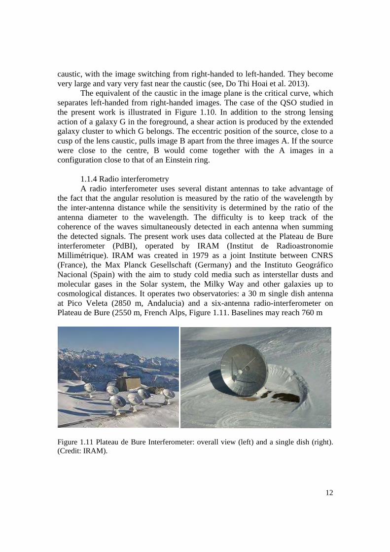
12

caustic, with the image switching from right-handed to left-handed. They become very large and vary very fast near the caustic (see, Do Thi Hoai et al. 2013). The equivalent of the caustic in the image plane is the critical curve, which separates left-handed from right-handed images. The case of the QSO studied in the present work is illustrated in Figure 1.10. In addition to the strong lensing action of a galaxy G in the foreground, a shear action is produced by the extended galaxy cluster to which G belongs. The eccentric position of the source, close to a cusp of the lens caustic, pulls image B apart from the three images A. If the source were close to the centre, B would come together with the A images in a configuration close to that of an Einstein ring.

1.1.4 Radio interferometry A radio interferometer uses several distant antennas to take advantage of

the fact that the angular resolution is measured by the ratio of the wavelength by the inter-antenna distance while the sensitivity is determined by the ratio of the antenna diameter to the wavelength. The difficulty is to keep track of the coherence of the waves simultaneously detected in each antenna when summing the detected signals. The present work uses data collected at the Plateau de Bure interferometer (PdBI), operated by IRAM (Institut de Radioastronomie Millimétrique). IRAM was created in 1979 as a joint Institute between CNRS (France), the Max Planck Gesellschaft (Germany) and the Instituto Geográfico Nacional (Spain) with the aim to study cold media such as interstellar dusts and molecular gases in the Solar system, the Milky Way and other galaxies up to cosmological distances. It operates two observatories: a 30 m single dish antenna at Pico Veleta (2850 m, Andalucia) and a six-antenna radio-interferometer on Plateau de Bure (2550 m, French Alps, Figure 1.11. Baselines may reach 760 m

Figure 1.11 Plateau de Bure Interferometer: overall view (left) and a single dish (right). (Credit: IRAM).

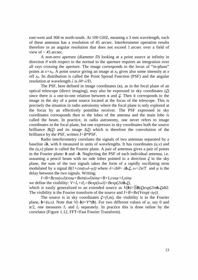
13

east-west and 368 m north-south. At 100 GHZ, meaning a 3 mm wavelength, each of these antennas has a resolution of 45 arcsec. Interferometer operation results therefore in an angular resolution that does not exceed 1 arcsec over a field of view of ~ 45 arcsec.

A non-zero aperture (diameter D) looking at a point source at infinity in direction θ with respect to the normal to the aperture requires an integration over all rays crossing the aperture. The image corresponds to the locus of “in-phase” points at x=x0. A point source giving an image at x0 gives also some intensity at x off x0. Its distribution is called the Point Spread Function (PSF) and the angular resolution at wavelength λ is δθ~λ/D.

The PSF, here defined in image coordinates (x), as in the focal plane of an optical telescope (direct imaging), may also be expressed in sky coordinates (ξ) since there is a one-to-one relation between x and ξ. Then it corresponds to the image in the sky of a point source located at the focus of the telescope. This is precisely the situation in radio astronomy where the focal plane is only explored at the focus by an effectively pointlike receiver. The PSF expressed in sky coordinates corresponds then to the lobes of the antenna and the main lobe is called the beam. In practice, in radio astronomy, one never refers to image coordinates in the focal plane, but one expresses in sky coordinates both the source brilliance B(ξ) and its image I(ξ) which is therefore the convolution of the brilliance by the PSF, written I=B*PSF.

Radio interferometry correlates the signals of two antennas separated by a baseline λb, with b measured in units of wavelengths. It has coordinates (u,v) and the (u,v) plane is called the Fourier plane. A pair of antennas gives a pair of points in the Fourier plane: b and –b. Neglecting the PSF of each individual antenna, i.e. assuming a pencil beam with no side lobes pointed to a direction ξ in the sky plane, the sum of the two signals takes the form of a rapidly oscillating term modulated by a signal B(1+cos(ωδ–φ)) where δ=λbθ~ λb.ξ, ω=2π/T and φ is the delay between the two signals. Writing;

I=B+Bcos(ωδ)cosφ+Bsin(ωδ)sinφ=B+I 1cosφ+I 2sinφ we define the visibility: V=I1+iI 2=Bexp(iωδ)=Bexp(2iπb.ξ), which is easily generalized to an extended source as V(b)= ∫∫B(ξ)exp(2iπb.ξ)dΩ. The visibility is the Fourier transform of the source and I=B+ReVexp(–iφ).

The source is in sky coordinates ξ=(l,m), the visibility is in the Fourier plane, b=(u,v). Note that V(–b)=V*(b). For two different values of φ, say 0 and π/2, one measures I1 and I2 separately. In practice this is done online by the correlator (Figure 1.12, FFT=Fast Fourier Transform).

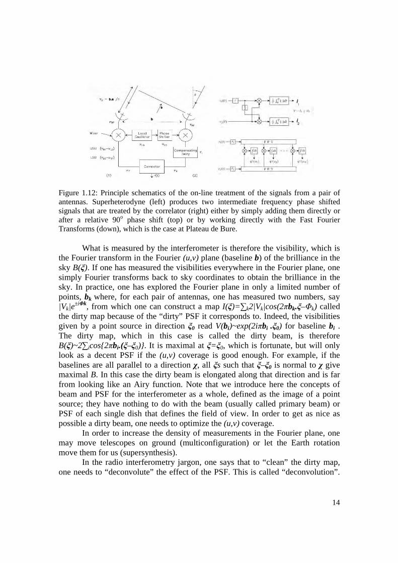
14

Figure 1.12: Principle schematics of the on-line treatment of the signals from a pair of antennas. Superheterodyne (left) produces two intermediate frequency phase shifted signals that are treated by the correlator (right) either by simply adding them directly or after a relative 90o phase shift (top) or by working directly with the Fast Fourier Transforms (down), which is the case at Plateau de Bure.

What is measured by the interferometer is therefore the visibility, which is

the Fourier transform in the Fourier (u,v) plane (baseline b) of the brilliance in the sky B(ξ). If one has measured the visibilities everywhere in the Fourier plane, one simply Fourier transforms back to sky coordinates to obtain the brilliance in the sky. In practice, one has explored the Fourier plane in only a limited number of points, bk where, for each pair of antennas, one has measured two numbers, say |Vk|e

±iΦk, from which one can construct a map I(ξ)=∑k2|Vk|cos(2πbk.ξ–Φk) called the dirty map because of the “dirty” PSF it corresponds to. Indeed, the visibilities given by a point source in direction ξ0 read V(bi)~exp(2iπbi .ξ0) for baseline bi . The dirty map, which in this case is called the dirty beam, is therefore B(ξ)~2∑icos2πbi.(ξ–ξ0). It is maximal at ξ=ξ0, which is fortunate, but will only look as a decent PSF if the (u,v) coverage is good enough. For example, if the baselines are all parallel to a direction χ, all ξs such that ξ–ξ0 is normal to χ give maximal B. In this case the dirty beam is elongated along that direction and is far from looking like an Airy function. Note that we introduce here the concepts of beam and PSF for the interferometer as a whole, defined as the image of a point source; they have nothing to do with the beam (usually called primary beam) or PSF of each single dish that defines the field of view. In order to get as nice as possible a dirty beam, one needs to optimize the (u,v) coverage.

In order to increase the density of measurements in the Fourier plane, one may move telescopes on ground (multiconfiguration) or let the Earth rotation move them for us (supersynthesis).

In the radio interferometry jargon, one says that to “clean” the dirty map, one needs to “deconvolute” the effect of the PSF. This is called “deconvolution”.

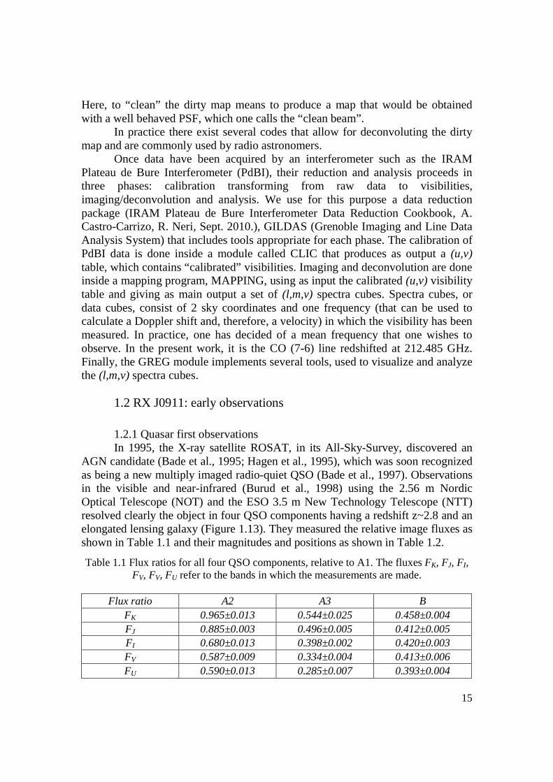
15

Here, to “clean” the dirty map means to produce a map that would be obtained with a well behaved PSF, which one calls the “clean beam”.

In practice there exist several codes that allow for deconvoluting the dirty map and are commonly used by radio astronomers.

Once data have been acquired by an interferometer such as the IRAM Plateau de Bure Interferometer (PdBI), their reduction and analysis proceeds in three phases: calibration transforming from raw data to visibilities, imaging/deconvolution and analysis. We use for this purpose a data reduction package (IRAM Plateau de Bure Interferometer Data Reduction Cookbook, A. Castro-Carrizo, R. Neri, Sept. 2010.), GILDAS (Grenoble Imaging and Line Data Analysis System) that includes tools appropriate for each phase. The calibration of PdBI data is done inside a module called CLIC that produces as output a (u,v) table, which contains “calibrated” visibilities. Imaging and deconvolution are done inside a mapping program, MAPPING, using as input the calibrated (u,v) visibility table and giving as main output a set of (l,m,v) spectra cubes. Spectra cubes, or data cubes, consist of 2 sky coordinates and one frequency (that can be used to calculate a Doppler shift and, therefore, a velocity) in which the visibility has been measured. In practice, one has decided of a mean frequency that one wishes to observe. In the present work, it is the CO (7-6) line redshifted at 212.485 GHz. Finally, the GREG module implements several tools, used to visualize and analyze the (l,m,v) spectra cubes.

1.2 RX J0911: early observations 1.2.1 Quasar first observations In 1995, the X-ray satellite ROSAT, in its All-Sky-Survey, discovered an

AGN candidate (Bade et al., 1995; Hagen et al., 1995), which was soon recognized as being a new multiply imaged radio-quiet QSO (Bade et al., 1997). Observations in the visible and near-infrared (Burud et al., 1998) using the 2.56 m Nordic Optical Telescope (NOT) and the ESO 3.5 m New Technology Telescope (NTT) resolved clearly the object in four QSO components having a redshift z~2.8 and an elongated lensing galaxy (Figure 1.13). They measured the relative image fluxes as shown in Table 1.1 and their magnitudes and positions as shown in Table 1.2.

Table 1.1 Flux ratios for all four QSO components, relative to A1. The fluxes FK, FJ, FI, FV, FV, FU refer to the bands in which the measurements are made.

Flux ratio A2 A3 B

FK 0.965±0.013 0.544±0.025 0.458±0.004 FJ 0.885±0.003 0.496±0.005 0.412±0.005 FI 0.680±0.013 0.398±0.002 0.420±0.003 FV 0.587±0.009 0.334±0.004 0.413±0.006 FU 0.590±0.013 0.285±0.007 0.393±0.004

16

Table 1.2 Photometric and astrometric properties of RX J0911 and the lensing galaxy

Magnitudes Positions

A1 A2 A3 B G

K 17.137±0.020 17.308±0.035 17.933±0.074 18.119±0.010 17.88±0.12 J 17.794±0.030 17.927±0.029 18.556±0.038 18.757±0.020 19.85±0.12 I 18.140±0.084 18.558±0.096 19.135±0.133 19.027±0.083 21.9±0.13

x (arcsec) 0±0.004 –0.259±0.007 0.013±0.008 2.935±0.002 0.709±0.026 y (arcsec) 0±0.008 0.402±0.006 0.946±0.008 0.785±0.003 0.507±0.046

Figure 1.13 High resolution images of RX J0911 before (left) and after (right) deconvolution. Upper panels: NOT/HIRAC (High Resolution Adaptive Camera) I-band images, 900 s exposure time; Middle panels: NTT/SOFI J-band images, 1080 s exposure time; Lower panels: NTT/SOFI K-band images, 2400 s exposure time. North is to the top and East to the left on all frames (Burud et al. 1998).

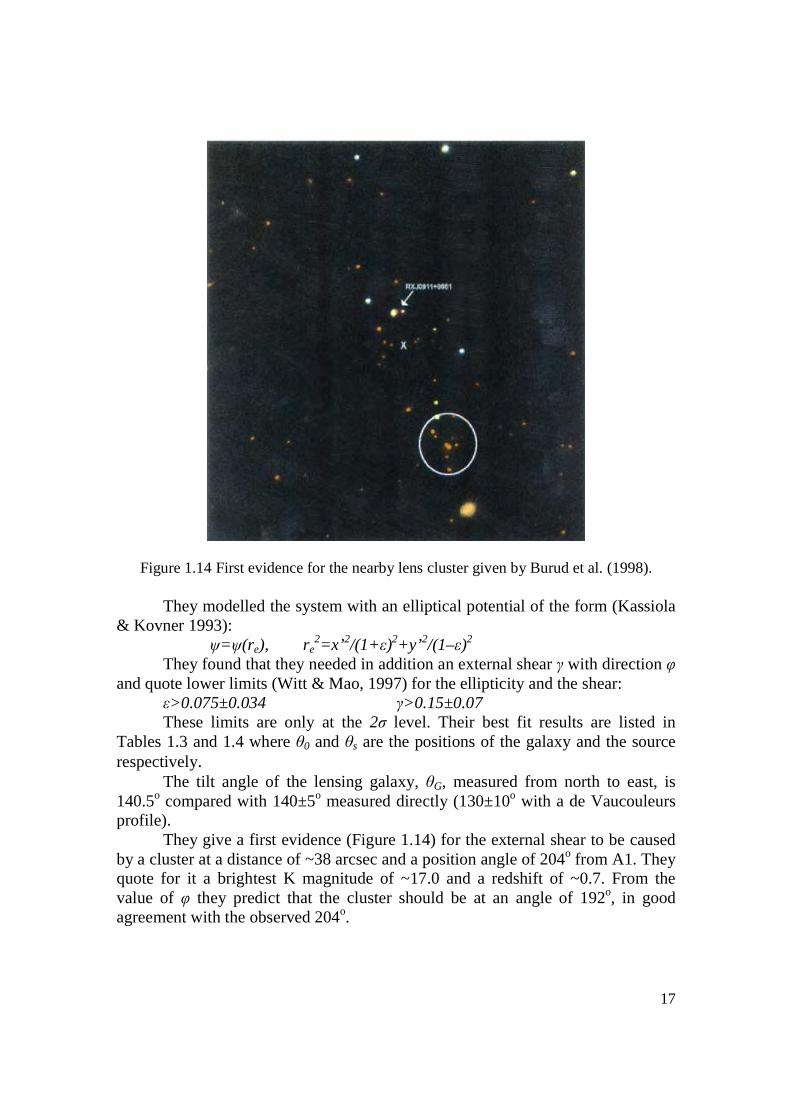
17

Figure 1.14 First evidence for the nearby lens cluster given by Burud et al. (1998).

They modelled the system with an elliptical potential of the form (Kassiola & Kovner 1993):

ψ=ψ(re), re2=x’ 2/(1+ε)2+y’ 2/(1–ε)2

They found that they needed in addition an external shear γ with direction φ and quote lower limits (Witt & Mao, 1997) for the ellipticity and the shear:

ε>0.075±0.034 γ>0.15±0.07 These limits are only at the 2σ level. Their best fit results are listed in

Tables 1.3 and 1.4 where θ0 and θs are the positions of the galaxy and the source respectively.

The tilt angle of the lensing galaxy, θG, measured from north to east, is 140.5o compared with 140±5o measured directly (130±10o with a de Vaucouleurs profile).

They give a first evidence (Figure 1.14) for the external shear to be caused by a cluster at a distance of ~38 arcsec and a position angle of 204o from A1. They quote for it a brightest K magnitude of ~17.0 and a redshift of ~0.7. From the value of φ they predict that the cluster should be at an angle of 192o, in good agreement with the observed 204o.

18

Table 1.3 Parameters of the best fit potential

α0 ε θG γ φ θ0 θs

1”1061 0.0476 140.5o 0.3176 102.3o 0.7078” 1.1459”

Table 1.4 Best fit image coordinates and magnifications

Image x y Magnification A1 0.0000 –0.0004” –4.45 A2 –0.2590” 0.4019” 8.59 A3 0.0130” 0.9456” –3.70 B 2.9350” 0.7850” 1.79

1.2.2 HST images, strong lensing and the cluster lens In 2000 the lens was identified as being a member of a galaxy cluster

(Figure 1.15 a) having a mean redshift z=0.769±0.002 and a velocity dispersion of 836±190 km/s using the Low Resolution Imaging Spectrograph of the Keck II Telescope (Kneib, Cohen & Jens Hjorth 2000). Both the originally discovered lens and the rest of the cluster contribute to gravitational lensing, the former in the form of strong lensing (multiple imaging), the second in the form of an external shear. They estimate the external shear to be ~0.11 to 0.13. They give a map of the cluster mass (Figure 1.15 b) and estimate its harmonic radius to be 632h–1 kpc, its mass to be ~6.2±2.7 1014 MSun and its X-ray temperature to be 4.5±1.2 keV. They quote the time delay between A and B to be between 190h–1 and 260h–1 days.

Two years later, Kochanek (2002) presents the result of a fit including CASTLES photometric data (see below, Kochanek et al. 2002), the time delay data (ABC vs D, 150±6 days) of Burud et al. (2002b) and the Morgan et al. (2001) centroid for the nearby X-ray cluster, 12.0”±3.0” East and –39.8”±3 South of image B. The lens galaxies were modelled by two de Vaucouleurs components. The primary lens has a major axis effective radius of 0.77” ±0.07” a major axis position angle of –39o±15o and an axis ratio of 0.79±0.06. The satellite galaxy (only 8% of the H band flux) has a major axis effective radius of 0.36”±0.14” and is indistinguishable from round in the available data.

The author notes that the lensing potential of the cluster has significant effects on the estimate of H0. He models the cluster as a single isothermal sphere (SIS), with equal shear and convergence, finding reasonable fits for cluster velocity dispersions at 1100 km/s for the dark matter models and 1250 km/s for the constant M/L models. The SIS models are in reasonable agreement with the 840±200 km/s velocity dispersion of the galaxies (Kneib et al. 2000, Burud 2002b).

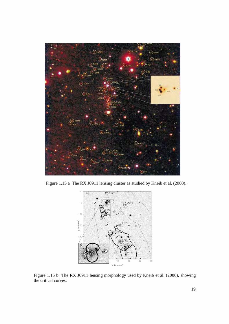
19

Figure 1.15 Figure 1.15 a The RX J0911 lensing cluster as studied by Kneib et al. (2000).

Figure 1.15 b The RX J0911 lensing morphology used by Kneib et al. (2000), showing the critical curves.

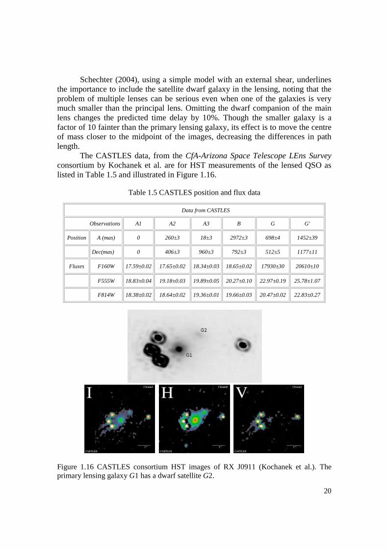
20

Schechter (2004), using a simple model with an external shear, underlines the importance to include the satellite dwarf galaxy in the lensing, noting that the problem of multiple lenses can be serious even when one of the galaxies is very much smaller than the principal lens. Omitting the dwarf companion of the main lens changes the predicted time delay by 10%. Though the smaller galaxy is a factor of 10 fainter than the primary lensing galaxy, its effect is to move the centre of mass closer to the midpoint of the images, decreasing the differences in path length.

The CASTLES data, from the CfA-Arizona Space Telescope LEns Survey consortium by Kochanek et al. are for HST measurements of the lensed QSO as listed in Table 1.5 and illustrated in Figure 1.16.

Table 1.5 CASTLES position and flux data

Data from CASTLES

Observations A1 A2 A3 B G G'

Position A (mas) 0 260±3 18±3 2972±3 698±4 1452±39

Dec(mas) 0 406±3 960±3 792±3 512±5 1177±11

Fluxes F160W 17.59±0.02 17.65±0.02 18.34±0.03 18.65±0.02 17930±30 20610±10

F555W 18.83±0.04 19.18±0.03 19.89±0.05 20.27±0.10 22.97±0.19 25.78±1.07

F814W 18.38±0.02 18.64±0.02 19.36±0.01 19.66±0.03 20.47±0.02 22.83±0.27

Figure 1.16 CASTLES consortium HST images of RX J0911 (Kochanek et al.). The primary lensing galaxy G1 has a dwarf satellite G2.

21

1.2.3 X-ray data and time delay X ray data (Figure 1.17) by CHANDRA (Morgan et al., 2001) give a

cluster temperature of 2.3 (+1.8/–0.8) keV and a 2-10 keV luminosity of 7.6 (+0.6/–0.2)1043 ergs.s-1. Remember that Kneib et al. (2000) predicted a temperature of 4.5±1.2 keV.

The X ray data have been used to measure time delays (Hjorth et al., 2002). The method consists in matching the occurrence of flares on different images by allowing for a time delay between the two. The A to B delay (Figure 1.17) was measured to be 146±6 days.

Figure 1.17 Left: Chandra data of the time dependence of the X-ray fluxes from images A1 and A2. Because of the time delay, the flare visible on A2 is not simultaneous with its companion on A1. Right: Combined light curve (Hjorth et al., 2002) from both components of RX J0911.4+0551. The curve of the A component is shifted forward in time by 146 days. The B curve has been offset by values between -1.95 mag and -2.05 mag.

They modelled the system as Kneib et al. (2000) using their measured velocity dispersion to constrain the cluster mass and adopted more realistic constraints on the ellipticity of the cluster mass distribution and a tighter mass-luminosity relation for the cluster galaxies. The main model uncertainty concerns

the value of the cluster convergence κ at the location of the multiple images. A large κ gives rise to a small predicted time delay and derived H0.

The value of κ is governed by the mass of the cluster, its mass profile, and the effects of possible

substructure in the cluster. They find that 0.20<κ<0.28 is required for a good fit. This range in κ translates into different values for the mass and velocity dispersion

of the cluster, depending on the mass profile used and the ellipticity of the cluster mass distribution. In addition to the smooth cluster convergence, there is a

22

contribution to the total convergence of about 0.06 from the individual galaxies in

the cluster (not including the main lens) (Hjorth et al., 2002).

The refined model prediction of the (flux-weighted or straight) mean B-A time delay is (104±11)h-1 days (the individual time delays between the A components are less than 1.5h-1 days, generally in the sequence A2, A1, A3). With the measured B-A time delay of 146±8 days (2σ), the resulting value of the Hubble constant is H0=71±4 (random, 2σ) ±8 (systematic) km s-1 Mpc-1. (Hjorth et al., 2002).

1.2.4 CO and other molecular data Recently, the CO(1-0) emission of RX J0911 was measured (Riechers et

al., 2011) using the EVLA (Expanded Very Large Array) (Figure 1.18). The images were not resolved. The authors quote a z of 2.7961±0.0001, a lens magnification factor of 22, a Sν of 1.20±0.15 mJy, a line FWHM of 111±19 km/s, an ICO of 0.205±0.029 Jy km/s and a L’ CO(1-0) (corrected for magnification by gravitational lensing) of 3.39±0.48 109 K km/s pc2. They state that the measured FWHM is in excellent agreement with the measurements (~110 km/s) of CO(3-2) to CO(9-8) produced by Weiss et al. (private communication). The latter are said to revise the CO(3-2) line flux and width measured by Hainline et al. (2004) down by ~40% and a factor of ~3 respectively. The rest-frame 2.6 mm continuum emission is not detected down to a 3σ limit of 170 µJy.

Weiss et al. (2012) report on a measurement of the CO(7-6) line using the PdBI. While the A images are not resolved (Figure 1.19), the detection of the CI line is made simultaneously to that of the CO line. They measure B/A =0.21±0.01 integrated on the CO line and use the similarity with the value measured at ~100 nm by Burud et al. (1998) as an argument to adopt the same magnification of 20.

Figure 1.18 Left: RX J0911 image from EVLA (Riechers et al. 2011). Right: the CO(1-0) line.

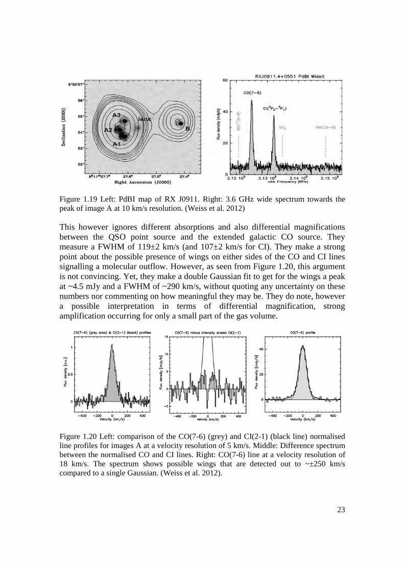
23

Figure 1.19 Left: PdBI map of RX J0911. Right: 3.6 GHz wide spectrum towards the peak of image A at 10 km/s resolution. (Weiss et al. 2012)

This however ignores different absorptions and also differential magnifications between the QSO point source and the extended galactic CO source. They measure a FWHM of 119±2 km/s (and 107±2 km/s for CI). They make a strong point about the possible presence of wings on either sides of the CO and CI lines signalling a molecular outflow. However, as seen from Figure 1.20, this argument is not convincing. Yet, they make a double Gaussian fit to get for the wings a peak at ~4.5 mJy and a FWHM of ~290 km/s, without quoting any uncertainty on these numbers nor commenting on how meaningful they may be. They do note, however a possible interpretation in terms of differential magnification, strong amplification occurring for only a small part of the gas volume.

Figure 1.20 Left: comparison of the CO(7-6) (grey) and CI(2-1) (black line) normalised line profiles for images A at a velocity resolution of 5 km/s. Middle: Difference spectrum between the normalised CO and CI lines. Right: CO(7-6) line at a velocity resolution of 18 km/s. The spectrum shows possible wings that are detected out to ~±250 km/s compared to a single Gaussian. (Weiss et al. 2012).

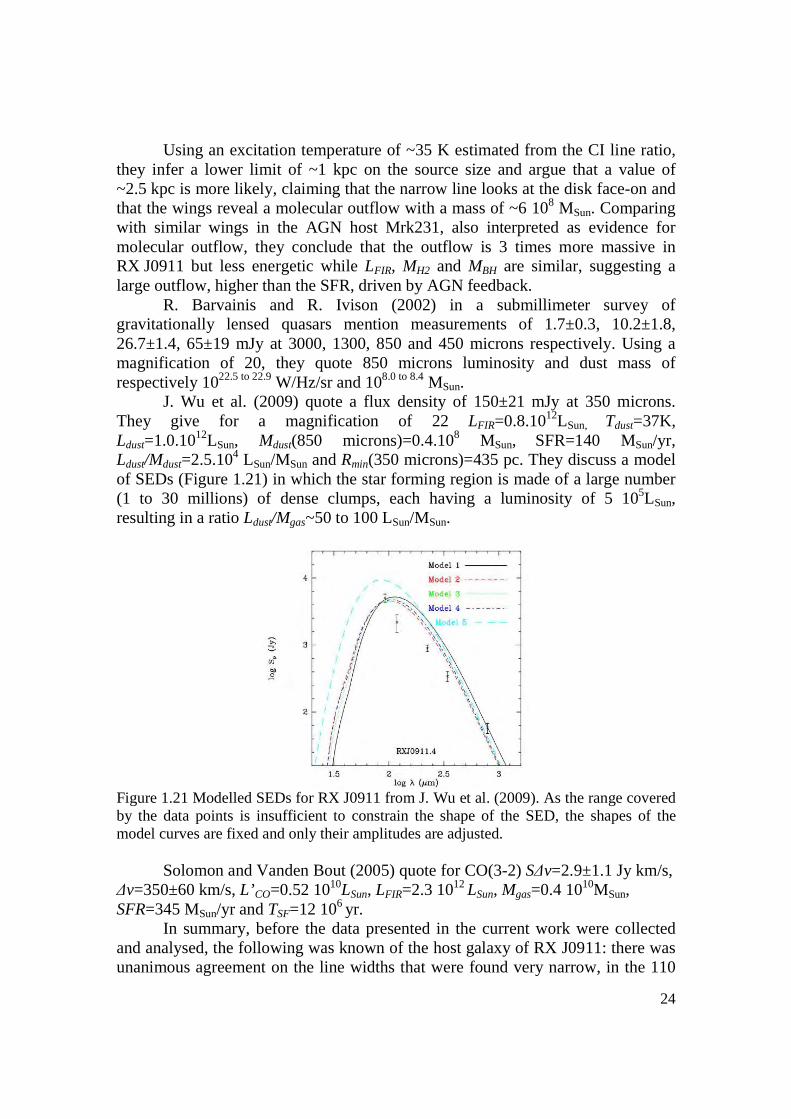
24

Using an excitation temperature of ~35 K estimated from the CI line ratio, they infer a lower limit of ~1 kpc on the source size and argue that a value of ~2.5 kpc is more likely, claiming that the narrow line looks at the disk face-on and that the wings reveal a molecular outflow with a mass of ~6 108 MSun. Comparing with similar wings in the AGN host Mrk231, also interpreted as evidence for molecular outflow, they conclude that the outflow is 3 times more massive in RX J0911 but less energetic while LFIR, MH2 and MBH are similar, suggesting a large outflow, higher than the SFR, driven by AGN feedback.

R. Barvainis and R. Ivison (2002) in a submillimeter survey of gravitationally lensed quasars mention measurements of 1.7±0.3, 10.2±1.8, 26.7±1.4, 65±19 mJy at 3000, 1300, 850 and 450 microns respectively. Using a magnification of 20, they quote 850 microns luminosity and dust mass of respectively 1022.5 to 22.9 W/Hz/sr and 108.0 to 8.4 MSun.

J. Wu et al. (2009) quote a flux density of 150±21 mJy at 350 microns. They give for a magnification of 22 LFIR=0.8.1012LSun, Tdust=37K, Ldust=1.0.1012LSun, Mdust(850 microns)=0.4.108 MSun, SFR=140 MSun/yr, Ldust/Mdust=2.5.104 LSun/MSun and Rmin(350 microns)=435 pc. They discuss a model of SEDs (Figure 1.21) in which the star forming region is made of a large number (1 to 30 millions) of dense clumps, each having a luminosity of 5 105LSun, resulting in a ratio Ldust/Mgas~50 to 100 LSun/MSun.

Figure 1.21 Modelled SEDs for RX J0911 from J. Wu et al. (2009). As the range covered by the data points is insufficient to constrain the shape of the SED, the shapes of the model curves are fixed and only their amplitudes are adjusted.

Solomon and Vanden Bout (2005) quote for CO(3-2) S∆v=2.9±1.1 Jy km/s, ∆v=350±60 km/s, L’ CO=0.52 1010LSun, LFIR=2.3 1012 LSun, Mgas=0.4 1010MSun, SFR=345 MSun/yr and TSF=12 106 yr.

In summary, before the data presented in the current work were collected and analysed, the following was known of the host galaxy of RX J0911: there was unanimous agreement on the line widths that were found very narrow, in the 110

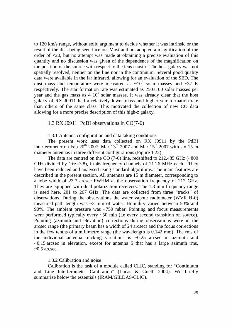
25

to 120 km/s range, without solid argument to decide whether it was intrinsic or the result of the disk being seen face on. Most authors adopted a magnification of the order of ×20, but no attempt was made at obtaining a precise evaluation of this quantity and no discussion was given of the dependence of the magnification on the position of the source with respect to the lens caustic. The host galaxy was not spatially resolved, neither on the line nor in the continuum. Several good quality data were available in the far infrared, allowing for an evaluation of the SED. The dust mass and temperature were measured as ~108 solar masses and ~37 K respectively. The star formation rate was estimated as 250±100 solar masses per year and the gas mass as 4 109 solar masses. It was already clear that the host galaxy of RX J0911 had a relatively lower mass and higher star formation rate than others of the same class. This motivated the collection of new CO data allowing for a more precise description of this high-z galaxy.

1.3 RX J0911: PdBI observations in CO(7-6)

1.3.1 Antenna configuration and data taking conditions The present work uses data collected on RX J0911 by the PdBI

interferometer on Feb 20th 2007, Mar 13rd 2007 and Mar 15th 2007 with six 15 m diameter antennas in three different configurations (Figure 1.22).

The data are centred on the CO (7-6) line, redshifted to 212.485 GHz (~800 GHz divided by 1+z=3.8), in 46 frequency channels of 21.26 MHz each. They have been reduced and analysed using standard algorithms. The main features are described in the present section. All antennas are 15 m diameter, corresponding to a lobe width of 23.7 arcsec FWHM at the observation frequency of 212 GHz. They are equipped with dual polarization receivers. The 1.3 mm frequency range is used here, 201 to 267 GHz. The data are collected from three “tracks” of observations. During the observations the water vapour radiometer (WVR H20) measured path length was ~3 mm of water. Humidity varied between 50% and 90%. The ambient pressure was ~750 mbar. Pointing and focus measurements were performed typically every ~50 min (i.e every second transition on source). Pointing (azimuth and elevation) corrections during observations were in the arcsec range (the primary beam has a width of 24 arcsec) and the focus corrections in the few tenths of a millimetre range (the wavelength is 0.142 mm). The rms of the individual antenna tracking variations is ~0.25 arcsec in azimuth and ~0.15 arcsec in elevation, except for antenna 5 that has a large azimuth rms, ~0.5 arcsec.

1.3.2 Calibration and noise Calibration is the task of a module called CLIC, standing for “Continuum

and Line Interferometer Calibration” (Lucas & Gueth 2004). We briefly summarize below the essentials (IRAM/GILDAS/CLIC).

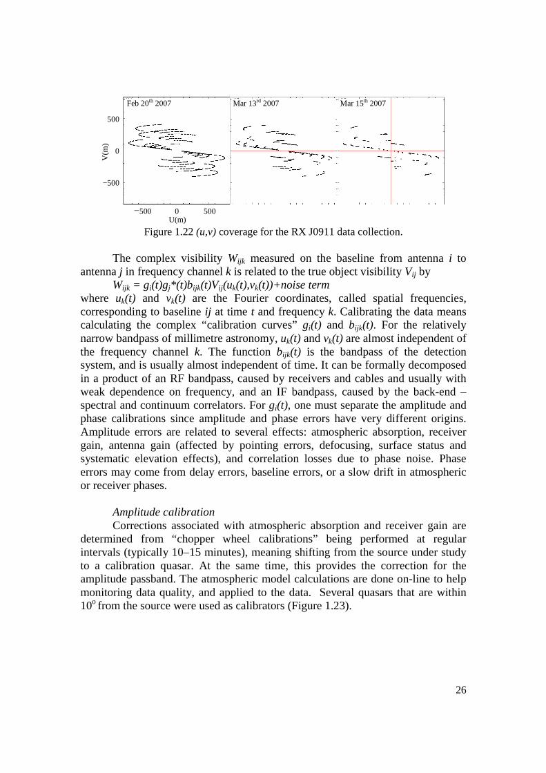
26

Figure 1.22 (u,v) coverage for the RX J0911 data collection.

The complex visibility Wijk measured on the baseline from antenna i to

antenna j in frequency channel k is related to the true object visibility Vij by Wijk = gi(t)gj*(t)b ijk(t)Vij(uk(t),vk(t))+noise term

where uk(t) and vk(t) are the Fourier coordinates, called spatial frequencies, corresponding to baseline ij at time t and frequency k. Calibrating the data means calculating the complex “calibration curves” gi(t) and bijk(t). For the relatively narrow bandpass of millimetre astronomy, uk(t) and vk(t) are almost independent of the frequency channel k. The function bijk(t) is the bandpass of the detection system, and is usually almost independent of time. It can be formally decomposed in a product of an RF bandpass, caused by receivers and cables and usually with weak dependence on frequency, and an IF bandpass, caused by the back-end – spectral and continuum correlators. For gi(t), one must separate the amplitude and phase calibrations since amplitude and phase errors have very different origins. Amplitude errors are related to several effects: atmospheric absorption, receiver gain, antenna gain (affected by pointing errors, defocusing, surface status and systematic elevation effects), and correlation losses due to phase noise. Phase errors may come from delay errors, baseline errors, or a slow drift in atmospheric or receiver phases.

Amplitude calibration Corrections associated with atmospheric absorption and receiver gain are

determined from “chopper wheel calibrations” being performed at regular intervals (typically 10–15 minutes), meaning shifting from the source under study to a calibration quasar. At the same time, this provides the correction for the amplitude passband. The atmospheric model calculations are done on-line to help monitoring data quality, and applied to the data. Several quasars that are within 10o from the source were used as calibrators (Figure 1.23).

500

0

−500

V(m

)

U(m)

Mar 15th 2007 Mar 13rd 2007 Feb 20th 2007

−500 0 500

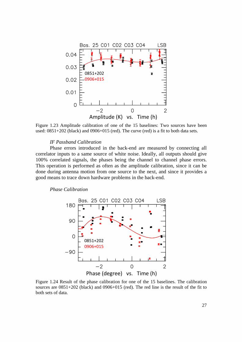
27

Figure 1.23 Amplitude calibration of one of the 15 baselines: Two sources have been used: 0851+202 (black) and 0906+015 (red). The curve (red) is a fit to both data sets.

IF Passband Calibration Phase errors introduced in the back-end are measured by connecting all

correlator inputs to a same source of white noise. Ideally, all outputs should give 100% correlated signals, the phases being the channel to channel phase errors. This operation is performed as often as the amplitude calibration, since it can be done during antenna motion from one source to the next, and since it provides a good means to trace down hardware problems in the back-end.

Phase Calibration

Figure 1.24 Result of the phase calibration for one of the 15 baselines. The calibration sources are 0851+202 (black) and 0906+015 (red). The red line is the result of the fit to both sets of data.

0851+202

0906+015

Phase (degree) vs. Time (h)

0851+202

0906+015

Amplitude (K) vs. Time (h)

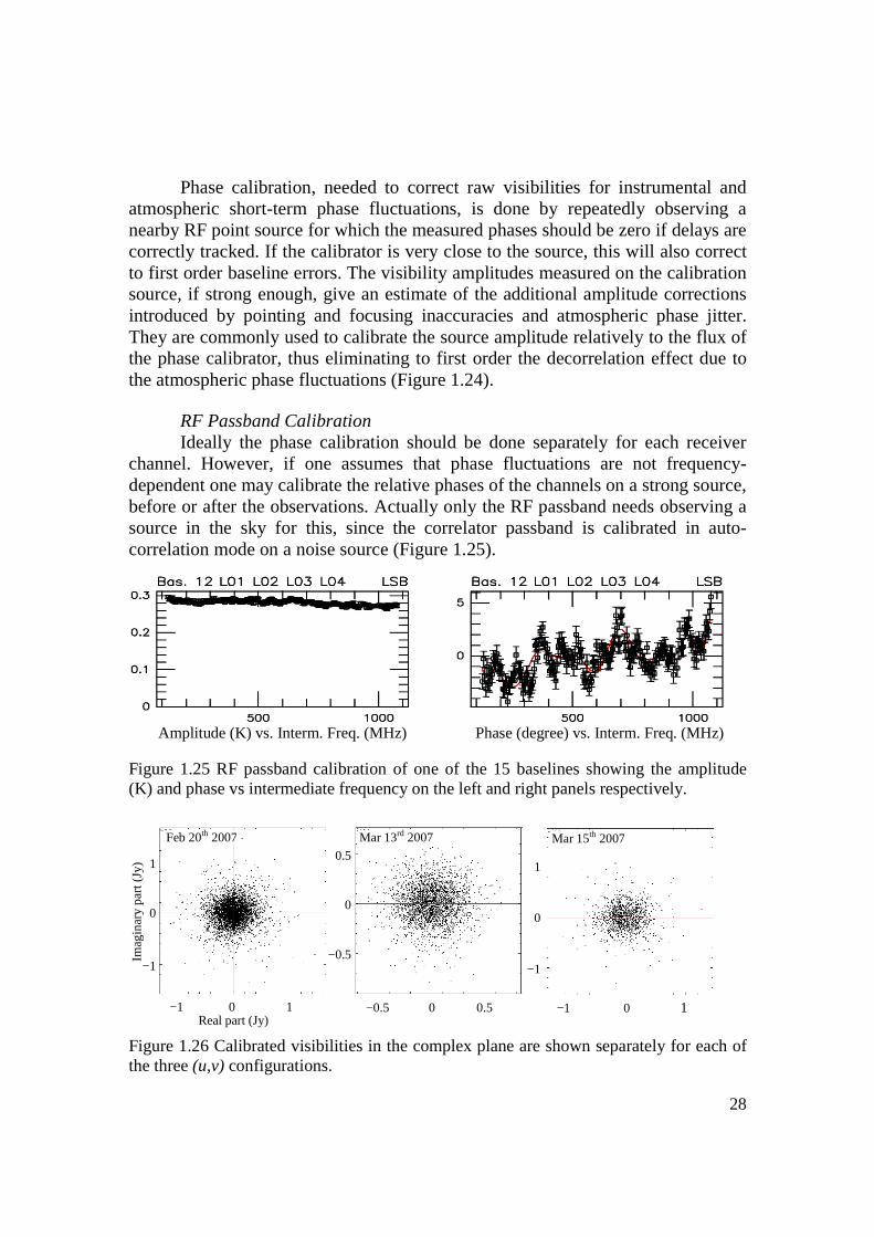
28

Phase calibration, needed to correct raw visibilities for instrumental and

atmospheric short-term phase fluctuations, is done by repeatedly observing a nearby RF point source for which the measured phases should be zero if delays are correctly tracked. If the calibrator is very close to the source, this will also correct to first order baseline errors. The visibility amplitudes measured on the calibration source, if strong enough, give an estimate of the additional amplitude corrections introduced by pointing and focusing inaccuracies and atmospheric phase jitter. They are commonly used to calibrate the source amplitude relatively to the flux of the phase calibrator, thus eliminating to first order the decorrelation effect due to the atmospheric phase fluctuations (Figure 1.24).

RF Passband Calibration Ideally the phase calibration should be done separately for each receiver

channel. However, if one assumes that phase fluctuations are not frequency-dependent one may calibrate the relative phases of the channels on a strong source, before or after the observations. Actually only the RF passband needs observing a source in the sky for this, since the correlator passband is calibrated in auto-correlation mode on a noise source (Figure 1.25).

Figure 1.25 RF passband calibration of one of the 15 baselines showing the amplitude (K) and phase vs intermediate frequency on the left and right panels respectively.

Figure 1.26 Calibrated visibilities in the complex plane are shown separately for each of the three (u,v) configurations.

−1 0 1

1

0

−1

Real part (Jy)

Imag

inar

y p

art

(Jy

)

−0.5 0 0.5

0.5

0

−0.5

1

0

−1

−1 0 1

Feb 20th 2007 Mar 13rd 2007 Mar 15th 2007

Amplitude (K) vs. Interm. Freq. (MHz) Phase (degree) vs. Interm. Freq. (MHz)

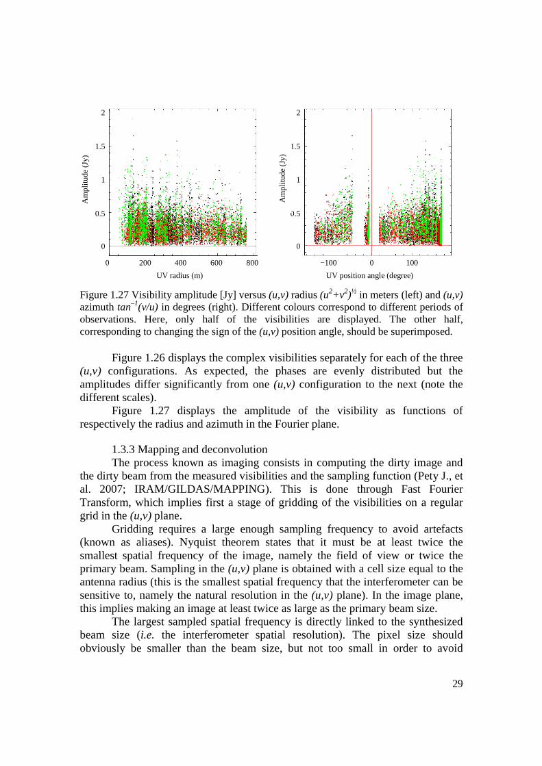
29

Figure 1.27 Visibility amplitude [Jy] versus (u,v) radius (u2+v2)½ in meters (left) and (u,v) azimuth tan–1(v/u) in degrees (right). Different colours correspond to different periods of observations. Here, only half of the visibilities are displayed. The other half, corresponding to changing the sign of the (u,v) position angle, should be superimposed.

Figure 1.26 displays the complex visibilities separately for each of the three

(u,v) configurations. As expected, the phases are evenly distributed but the amplitudes differ significantly from one (u,v) configuration to the next (note the different scales).

Figure 1.27 displays the amplitude of the visibility as functions of respectively the radius and azimuth in the Fourier plane.

1.3.3 Mapping and deconvolution The process known as imaging consists in computing the dirty image and

the dirty beam from the measured visibilities and the sampling function (Pety J., et al. 2007; IRAM/GILDAS/MAPPING). This is done through Fast Fourier Transform, which implies first a stage of gridding of the visibilities on a regular grid in the (u,v) plane.

Gridding requires a large enough sampling frequency to avoid artefacts (known as aliases). Nyquist theorem states that it must be at least twice the smallest spatial frequency of the image, namely the field of view or twice the primary beam. Sampling in the (u,v) plane is obtained with a cell size equal to the antenna radius (this is the smallest spatial frequency that the interferometer can be sensitive to, namely the natural resolution in the (u,v) plane). In the image plane, this implies making an image at least twice as large as the primary beam size.

The largest sampled spatial frequency is directly linked to the synthesized beam size (i.e. the interferometer spatial resolution). The pixel size should obviously be smaller than the beam size, but not too small in order to avoid

Am

plit

ud

e (J

y)

0 200 400 600 800

2

1.5

1

0.5

0

2

1.5

1

0.5

0

−100 0 100 60800UV position angle (degree) UV radius (m)

Am

plit

ud

e (J

y)

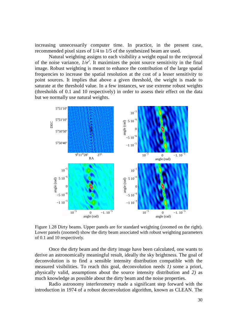
30

increasing unnecessarily computer time. In practice, in the present case, recommended pixel sizes of 1/4 to 1/5 of the synthesized beam are used.

Natural weighting assigns to each visibility a weight equal to the reciprocal of the noise variance, 1/σ2. It maximizes the point source sensitivity in the final image. Robust weighting is meant to enhance the contribution of the large spatial frequencies to increase the spatial resolution at the cost of a lesser sensitivity to point sources. It implies that above a given threshold, the weight is made to saturate at the threshold value. In a few instances, we use extreme robust weights (thresholds of 0.1 and 10 respectively) in order to assess their effect on the data but we normally use natural weights.

Figure 1.28 Dirty beams. Upper panels are for standard weighting (zoomed on the right). Lower panels (zoomed) show the dirty beam associated with robust weighting parameters of 0.1 and 10 respectively.

Once the dirty beam and the dirty image have been calculated, one wants to derive an astronomically meaningful result, ideally the sky brightness. The goal of deconvolution is to find a sensible intensity distribution compatible with the measured visibilities. To reach this goal, deconvolution needs 1) some a priori, physically valid, assumptions about the source intensity distribution and 2) as much knowledge as possible about the dirty beam and the noise properties.

Radio astronomy interferometry made a significant step forward with the introduction in 1974 of a robust deconvolution algorithm, known as CLEAN. The

9h11m28s 27s RA

5o51'10''

5o51'10''

5o50'50''

5o50'40''

DE

C

10−5

5 10−6

0

−5 10−6

−1 10−5

ang

le (

rad

)

angle (rad) 10

−5 0 −1. 10

−5

angle (rad) 10

−5 0 −1. 10

−5

angle (rad) 10

−5 0 −1. 10

−5

10−5

5 10−6

0

−5 10−6

−1 10−5

ang

le (

rad

)

10−5

5 10−6

0

−5 10−6

−1 10−5

ang

le (

rad

)

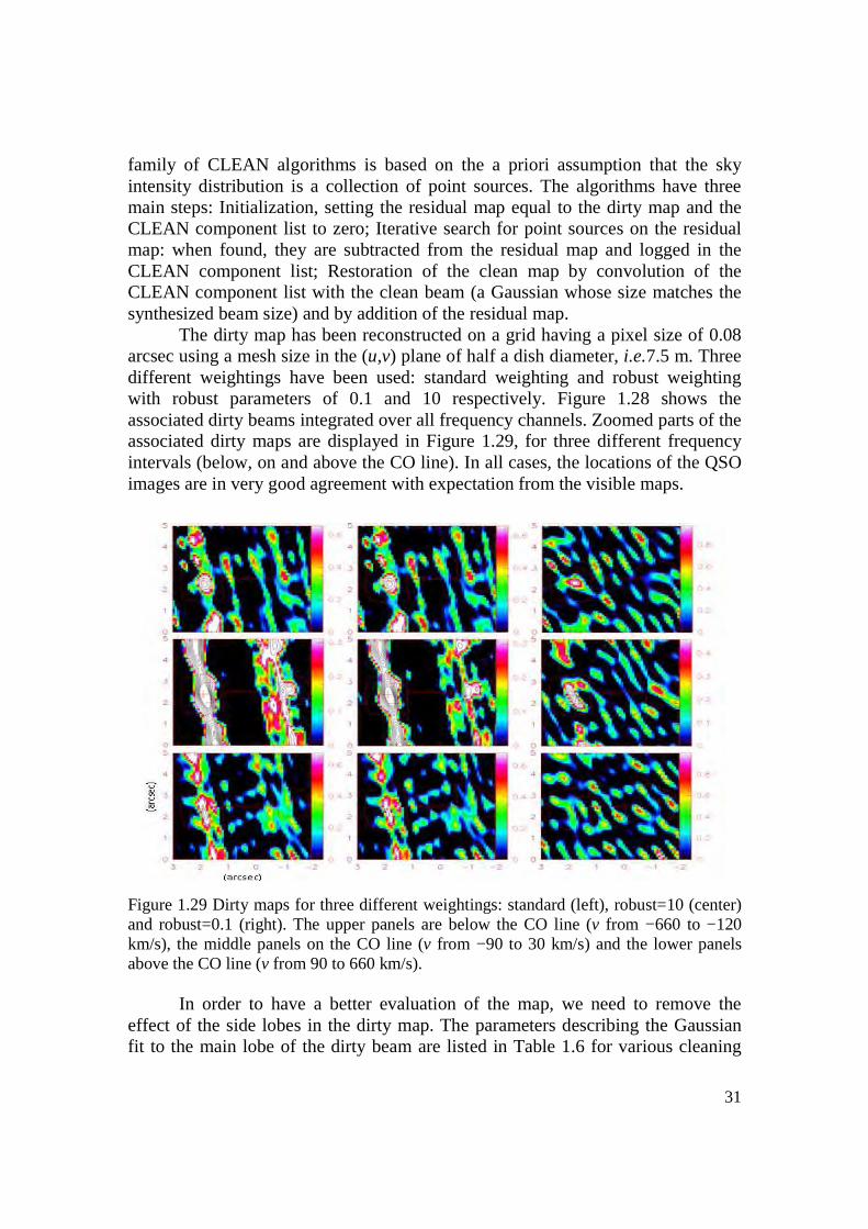
31

family of CLEAN algorithms is based on the a priori assumption that the sky intensity distribution is a collection of point sources. The algorithms have three main steps: Initialization, setting the residual map equal to the dirty map and the CLEAN component list to zero; Iterative search for point sources on the residual map: when found, they are subtracted from the residual map and logged in the CLEAN component list; Restoration of the clean map by convolution of the CLEAN component list with the clean beam (a Gaussian whose size matches the synthesized beam size) and by addition of the residual map.

The dirty map has been reconstructed on a grid having a pixel size of 0.08 arcsec using a mesh size in the (u,v) plane of half a dish diameter, i.e.7.5 m. Three different weightings have been used: standard weighting and robust weighting with robust parameters of 0.1 and 10 respectively. Figure 1.28 shows the associated dirty beams integrated over all frequency channels. Zoomed parts of the associated dirty maps are displayed in Figure 1.29, for three different frequency intervals (below, on and above the CO line). In all cases, the locations of the QSO images are in very good agreement with expectation from the visible maps.

Figure 1.29 Dirty maps for three different weightings: standard (left), robust=10 (center) and robust=0.1 (right). The upper panels are below the CO line (v from −660 to −120 km/s), the middle panels on the CO line (v from −90 to 30 km/s) and the lower panels above the CO line (v from 90 to 660 km/s).

In order to have a better evaluation of the map, we need to remove the effect of the side lobes in the dirty map. The parameters describing the Gaussian fit to the main lobe of the dirty beam are listed in Table 1.6 for various cleaning

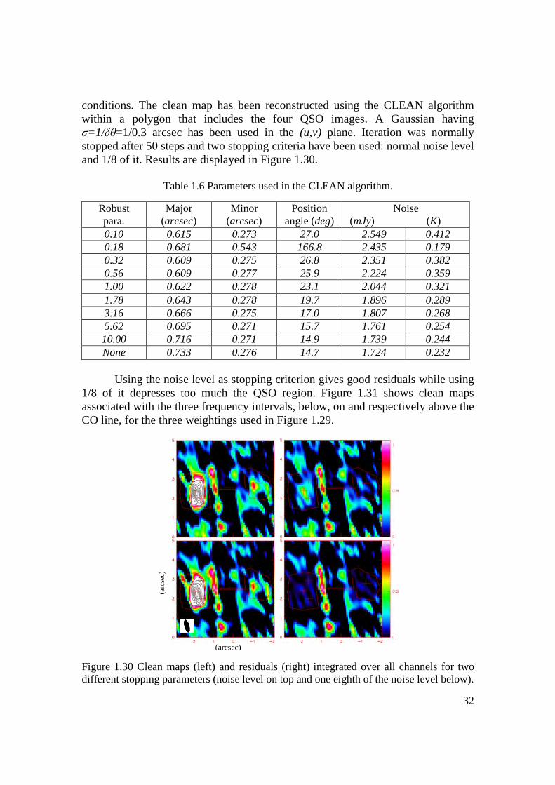
32

conditions. The clean map has been reconstructed using the CLEAN algorithm within a polygon that includes the four QSO images. A Gaussian having σ=1/δθ=1/0.3 arcsec has been used in the (u,v) plane. Iteration was normally stopped after 50 steps and two stopping criteria have been used: normal noise level and 1/8 of it. Results are displayed in Figure 1.30.

Table 1.6 Parameters used in the CLEAN algorithm.

Robust para.

Major (arcsec)

Minor (arcsec)

Position angle (deg)

Noise (mJy) (K)

0.10 0.615 0.273 27.0 2.549 0.412 0.18 0.681 0.543 166.8 2.435 0.179 0.32 0.609 0.275 26.8 2.351 0.382 0.56 0.609 0.277 25.9 2.224 0.359 1.00 0.622 0.278 23.1 2.044 0.321 1.78 0.643 0.278 19.7 1.896 0.289 3.16 0.666 0.275 17.0 1.807 0.268 5.62 0.695 0.271 15.7 1.761 0.254 10.00 0.716 0.271 14.9 1.739 0.244 None 0.733 0.276 14.7 1.724 0.232

Using the noise level as stopping criterion gives good residuals while using

1/8 of it depresses too much the QSO region. Figure 1.31 shows clean maps associated with the three frequency intervals, below, on and respectively above the CO line, for the three weightings used in Figure 1.29.

Figure 1.30 Clean maps (left) and residuals (right) integrated over all channels for two different stopping parameters (noise level on top and one eighth of the noise level below).

(arcsec)

(arc

sec)

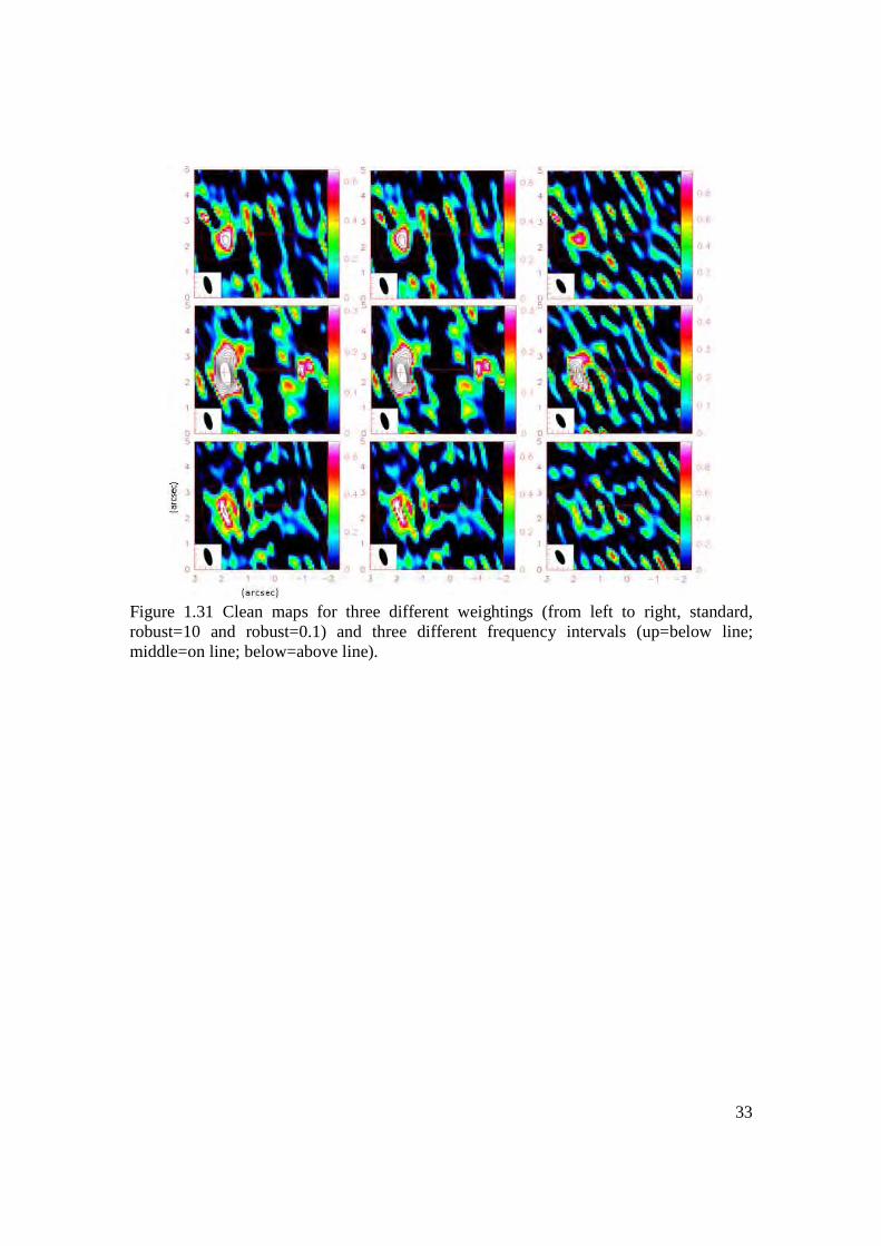
33

Figure 1.31 Clean maps for three different weightings (from left to right, standard, robust=10 and robust=0.1) and three different frequency intervals (up=below line; middle=on line; below=above line).

34

2. Gravitational lensing of QSO RX J0911

2.1 Introduction Strong gravitational lensing has been extensively studied and has become a

textbook topic. In particular, several authors, such as Blandford & al. (1989) or Saha & Williams (2003), have summarized the main properties in simple terms, underlining the most general qualitative features. While the case of complex lens configurations has been extensively studied (see for example Jullo & al. 2007), in particular with the aim of evaluating the mass distribution of baryonic and dark matter in cluster lenses, studies of strongly lensed extended sources are less common. The clearest cases of strong lensing, which are naturally the most extensively studied, are associated with sources located near the inner caustic of the lens, where magnifications are larger, making the problem highly non-linear: when crossing the caustic outward, magnifications become infinite and one switches from a four-image to a two-image configuration. Several authors, such as Dominik (1988), Bartelmann (2003), Suyu & Blandford (2005) or Suyu et al. (2009) have analysed the consequences in the case of extended sources and have described their effects in some detail. Such configurations will become more common with the completion of high sensitivity and angular resolution instruments, such as the Atacama Millimeter/Submillimeter Array (ALMA) or the Square Kilometer Array (SKA): the study of host galaxies of high redshift gravitationally lensed quasars will enter a new phase with the ability of resolving spatially the sources in both their molecular gas and dust contents.

The lensing of RX J0911, the quasar which is the subject of the present work, has been modelled as soon as discovered (Burud & al. 1998), requiring the presence of an important external shear in addition to the lens ellipticity. Two years later, the lens was identified by Kneib & al. (2000) as being a member of a galaxy cluster having a mean redshift z=0.769±0.002 and a velocity dispersion of 836±190 kms–1 using the Low Resolution Imaging Spectrograph of the Keck II Telescope. The cluster, with an estimated mass of ~6.2±2.7 1014 solar masses, is thought to be the main cause of the external shear.

The present chapter reviews and studies in detail the main features of the gravitational lensing of this quasar.

2.2 Strong lensing: a reminder 2.2.1 General formalism Fermat principle states that images form where the gradient of the time

delay, τ, cancels. In the approximation of small deflections, which always applies in practice, the time delay can be written as the sum of a geometrical delay and of the gravitational delay proper: τ =τ0(½[i–s] 2–ψ). Here, i and s are the image and source vectors in sky coordinates (angular distances measured in a plane normal to the line of sight), τ0 is a constant time scale and ψ is an effective potential that

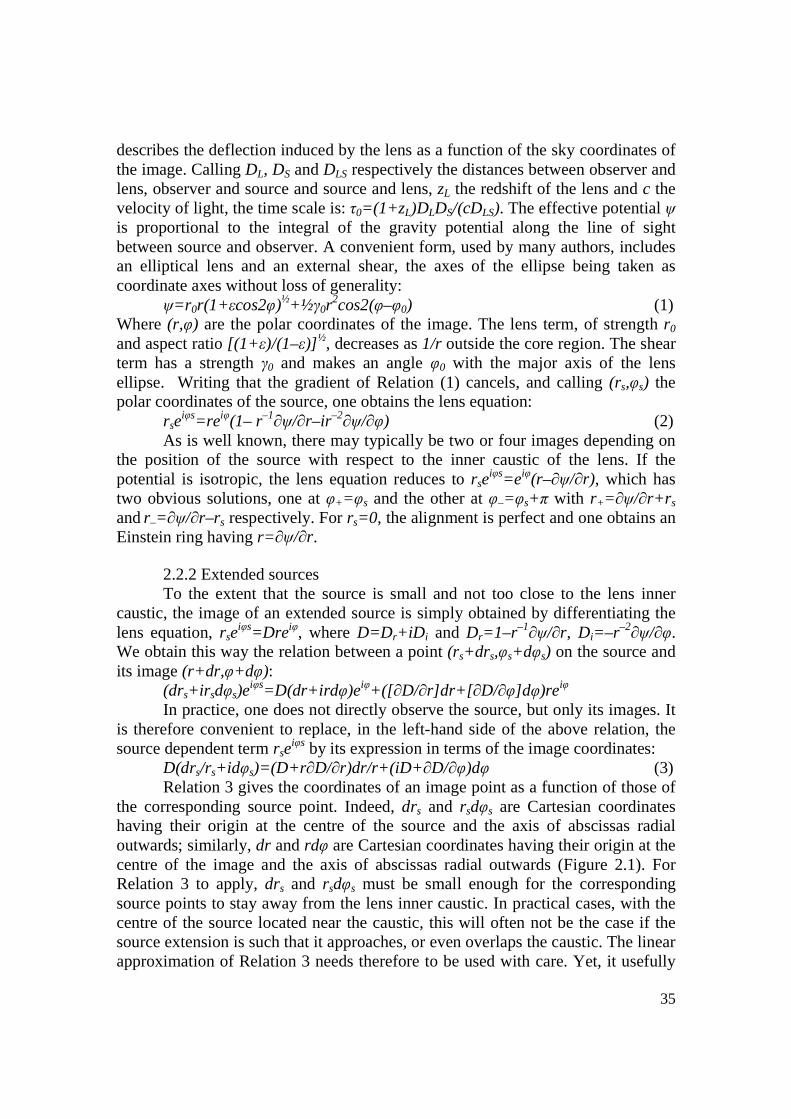
35

describes the deflection induced by the lens as a function of the sky coordinates of the image. Calling DL, DS and DLS respectively the distances between observer and lens, observer and source and source and lens, zL the redshift of the lens and c the velocity of light, the time scale is: τ0=(1+zL)DLDS/(cDLS). The effective potential ψ is proportional to the integral of the gravity potential along the line of sight between source and observer. A convenient form, used by many authors, includes an elliptical lens and an external shear, the axes of the ellipse being taken as coordinate axes without loss of generality:

ψ=r 0r(1+εcos2φ)½+½γ0r2cos2(φ–φ0) (1)

Where (r,φ) are the polar coordinates of the image. The lens term, of strength r0 and aspect ratio [(1+ ε)/(1–ε)] ½, decreases as 1/r outside the core region. The shear term has a strength γ0 and makes an angle φ0 with the major axis of the lens ellipse. Writing that the gradient of Relation (1) cancels, and calling (rs,φs) the polar coordinates of the source, one obtains the lens equation:

rseiφs=reiφ(1– r–1∂ψ/∂r–ir–2∂ψ/∂φ) (2)

As is well known, there may typically be two or four images depending on the position of the source with respect to the inner caustic of the lens. If the potential is isotropic, the lens equation reduces to rse

iφs=eiφ(r–∂ψ/∂r), which has two obvious solutions, one at φ+=φ s and the other at φ–=φs+π with r+=∂ψ /∂r+r s and r–=∂ψ /∂r–rs respectively. For rs=0, the alignment is perfect and one obtains an Einstein ring having r=∂ψ/∂r.

2.2.2 Extended sources To the extent that the source is small and not too close to the lens inner caustic, the image of an extended source is simply obtained by differentiating the lens equation, rse

iφs=Dreiφ, where D=D r+iD i and Dr=1–r–1∂ψ/∂r, Di=–r–2∂ψ/∂φ. We obtain this way the relation between a point (rs+drs,φs+dφs) on the source and its image (r+dr,φ+dφ):

(drs+ir sdφs)eiφs=D(dr+ird φ)eiφ+([∂ D/∂r]dr+[ ∂D/∂φ]dφ)reiφ

In practice, one does not directly observe the source, but only its images. It is therefore convenient to replace, in the left-hand side of the above relation, the source dependent term rse

iφs by its expression in terms of the image coordinates: D(drs/rs+idφs)=(D+r ∂D/∂r)dr/r+(iD+ ∂D/∂φ)dφ (3) Relation 3 gives the coordinates of an image point as a function of those of the corresponding source point. Indeed, drs and rsdφs are Cartesian coordinates having their origin at the centre of the source and the axis of abscissas radial outwards; similarly, dr and rdφ are Cartesian coordinates having their origin at the centre of the image and the axis of abscissas radial outwards (Figure 2.1). For Relation 3 to apply, drs and rsdφs must be small enough for the corresponding source points to stay away from the lens inner caustic. In practical cases, with the centre of the source located near the caustic, this will often not be the case if the source extension is such that it approaches, or even overlaps the caustic. The linear approximation of Relation 3 needs therefore to be used with care. Yet, it usefully

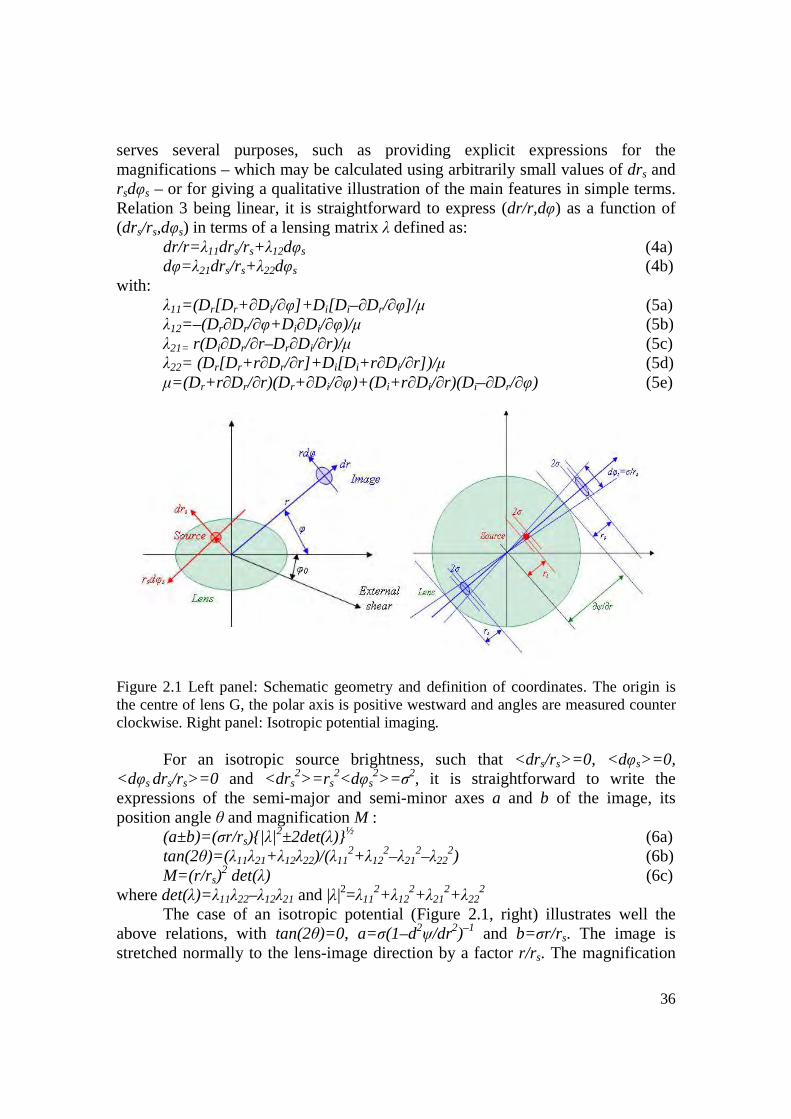
36

serves several purposes, such as providing explicit expressions for the magnifications – which may be calculated using arbitrarily small values of drs and rsdφs – or for giving a qualitative illustration of the main features in simple terms. Relation 3 being linear, it is straightforward to express (dr/r,dφ) as a function of (drs/rs,dφs) in terms of a lensing matrix λ defined as:

dr/r= λ11drs/rs+λ12dφs (4a) dφ=λ21drs/rs+λ22dφs (4b)

with: λ11=(D r[D r+∂Di/∂φ]+D i[D i–∂Dr/∂φ]/µ (5a) λ12=–(Dr∂Dr/∂φ+D i∂Di/∂φ)/µ (5b) λ21= r(Di∂Dr/∂r–Dr∂Di/∂r)/µ (5c) λ22= (Dr[D r+r∂Dr/∂r]+D i[D i+r∂Di/∂r])/µ (5d) µ=(D r+r∂Dr/∂r)(Dr+∂Di/∂φ)+(D i+r∂Di/∂r)(D i–∂Dr/∂φ) (5e)

Figure 2.1 Left panel: Schematic geometry and definition of coordinates. The origin is the centre of lens G, the polar axis is positive westward and angles are measured counter clockwise. Right panel: Isotropic potential imaging.

For an isotropic source brightness, such that <drs/rs>=0, <dφs>=0,

<dφs drs/rs>=0 and <drs2>=r s

2<dφs2>=σ 2, it is straightforward to write the

expressions of the semi-major and semi-minor axes a and b of the image, its position angle θ and magnification M : (a±b)=(σr/r s)|λ|

2±2det(λ)½ (6a) tan(2θ)=(λ11λ21+λ12λ22)/(λ11

2+λ122–λ21

2–λ222) (6b)

M=(r/r s)2 det(λ) (6c)

where det(λ)=λ11λ22–λ12λ21 and |λ|2=λ112+λ12

2+λ212+λ22

2 The case of an isotropic potential (Figure 2.1, right) illustrates well the

above relations, with tan(2θ)=0, a=σ(1–d2ψ/dr2)–1 and b=σr/r s. The image is stretched normally to the lens-image direction by a factor r/r s. The magnification

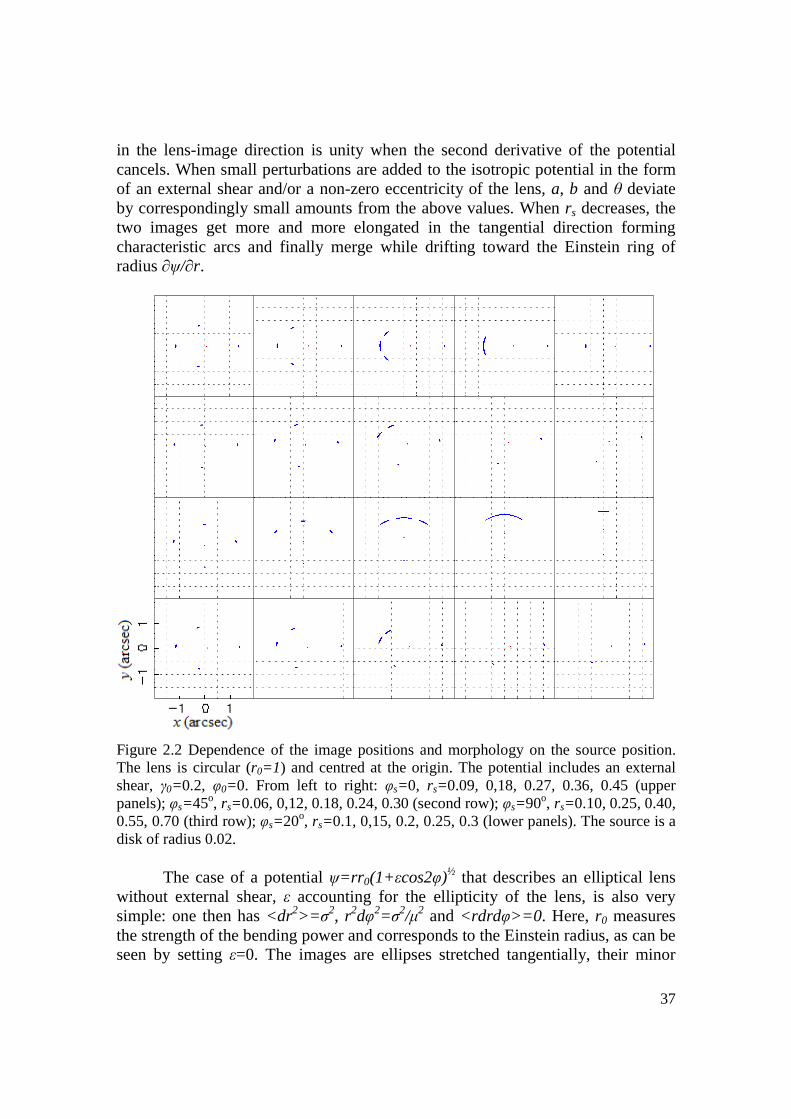
37

in the lens-image direction is unity when the second derivative of the potential cancels. When small perturbations are added to the isotropic potential in the form of an external shear and/or a non-zero eccentricity of the lens, a, b and θ deviate by correspondingly small amounts from the above values. When rs decreases, the two images get more and more elongated in the tangential direction forming characteristic arcs and finally merge while drifting toward the Einstein ring of radius ∂ψ/∂r.

Figure 2.2 Dependence of the image positions and morphology on the source position. The lens is circular (r0=1) and centred at the origin. The potential includes an external shear, γ0=0.2, φ0=0. From left to right: φs=0, rs=0.09, 0,18, 0.27, 0.36, 0.45 (upper panels); φs=45o, rs=0.06, 0,12, 0.18, 0.24, 0.30 (second row); φs=90o, rs=0.10, 0.25, 0.40, 0.55, 0.70 (third row); φs=20o, rs=0.1, 0,15, 0.2, 0.25, 0.3 (lower panels). The source is a disk of radius 0.02.

The case of a potential ψ=rr 0(1+εcos2φ)½ that describes an elliptical lens without external shear, ε accounting for the ellipticity of the lens, is also very simple: one then has <dr2>=σ 2, r2dφ2=σ2/µ2 and <rdrdφ>=0 . Here, r0 measures the strength of the bending power and corresponds to the Einstein radius, as can be seen by setting ε=0. The images are ellipses stretched tangentially, their minor

38

axes are equal to the source diameter and, writing µ=1–r0r–1(1–ε2)(1+εcos2φ)–3/2,

their major axes are a factor 1/µ larger. At constant φ, 1/µ is of the form r/(r–kr0) with k=(1–ε2)(1+εcos2φ)–3/2: it reaches unity at large values of r and increases when r decreases toward the critical curve, of equation r=kr 0, where 1/µ diverges.

Figure 2.3 Image appearances for the same potential and source size as in Figure 2.2. Source positions are: φs=20o, rs=0.1, 0,15, 0.2, 0.25, 0.3 from left to right. Images are drawn in (dr (up), rdφ (left)) coordinates. Images 1 to 4, numbered from South clockwise, are displayed in the upper to lower rows respectively.

Similar results are obtained for a potential of the form ψ=r 0r+½γ0r2cos2φ

that describes a circular lens with external shear along the axis of abscissas. Figure 2.2 shows how the positions of the images vary as a function of the source position with respect to the caustic: one switches from a four-image configuration, when the source is inside the caustic, to a two-image configuration, when the source is outside the caustic. Image shapes, illustrated in Figure 2.3 for different source positions, are again ellipses stretched tangentially but, at variance with the preceding case, they are slightly tilted as soon as φs deviates from 0o or 90o. Indeed, in the limit where γ0 is small and where the source is not too close to the inner caustic of the lens, one finds:

a=σ(1–γ0cos2φr0/(r–r0)), b=σr/(r–r 0) and tan(2θ)=(r/r 0)γ0sin2φ(1+2r2γ0cos2φ/(r0[r–r 0]) ; For γ0=0, as expected, the position angle cancels, the image has the same

radial size as the source and is stretched tangentially by a factor r/r s=r/(r–r 0).

dr

rdφ

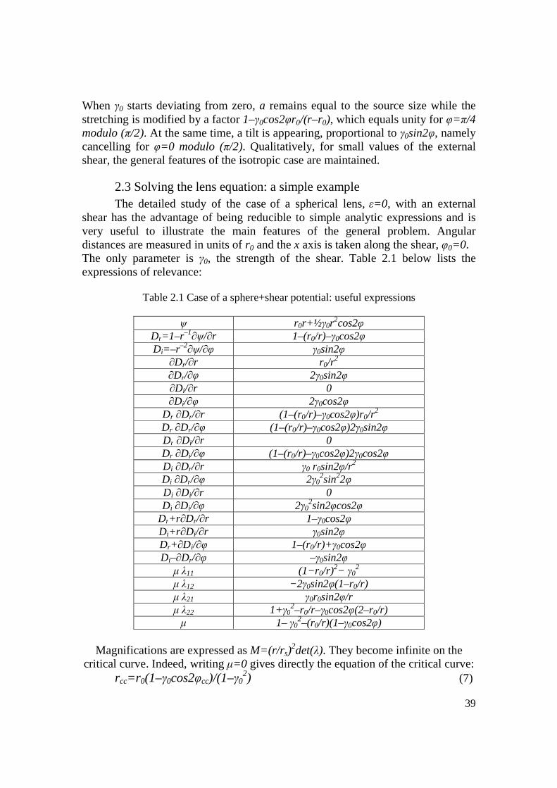
39

When γ0 starts deviating from zero, a remains equal to the source size while the stretching is modified by a factor 1–γ0cos2φr0/(r–r0), which equals unity for φ=π /4 modulo (π/2). At the same time, a tilt is appearing, proportional to γ0sin2φ, namely cancelling for φ=0 modulo (π/2). Qualitatively, for small values of the external shear, the general features of the isotropic case are maintained.

2.3 Solving the lens equation: a simple example

The detailed study of the case of a spherical lens, ε=0, with an external shear has the advantage of being reducible to simple analytic expressions and is very useful to illustrate the main features of the general problem. Angular distances are measured in units of r0 and the x axis is taken along the shear, φ0=0. The only parameter is γ0, the strength of the shear. Table 2.1 below lists the expressions of relevance:

Table 2.1 Case of a sphere+shear potential: useful expressions

ψ r0r+½γ0r

2cos2φ Dr=1–r–1∂ψ/∂r 1–(r0/r)–γ0cos2φ Di=–r–2∂ψ/∂φ γ0sin2φ

∂Dr/∂r r0/r2

∂Dr/∂φ 2γ0sin2φ ∂Di/∂r 0 ∂Di/∂φ 2γ0cos2φ

Dr ∂Dr/∂r (1–(r0/r)–γ0cos2φ)r0/r2

Dr ∂Dr/∂φ (1–(r0/r)–γ0cos2φ)2γ0sin2φ Dr ∂Di/∂r 0 Dr ∂Di/∂φ (1–(r0/r)–γ0cos2φ)2γ0cos2φ Di ∂Dr/∂r γ0 r0sin2φ/r2 Di ∂Dr/∂φ 2γ0

2sin22φ Di ∂Di/∂r 0 Di ∂Di/∂φ 2γ0

2sin2φcos2φ Dr+r∂Dr/∂r 1–γ0cos2φ Di+r∂Di/∂r γ0sin2φ Dr+∂Di/∂φ 1–(r0/r)+ γ0cos2φ Di–∂Dr/∂φ –γ0sin2φ

µ λ11 (1−r0/r)2− γ0

2 µ λ12 −2γ0sin2φ(1–r0/r) µ λ21 γ0r0sin2φ/r µ λ22 1+γ0

2–r0/r–γ0cos2φ(2–r0/r) µ 1– γ0

2–(r0/r)(1–γ0cos2φ)

Magnifications are expressed as M=(r/rs)2det(λ). They become infinite on the

critical curve. Indeed, writing µ=0 gives directly the equation of the critical curve: rcc=r 0(1–γ0cos2φcc)/(1–γ0

2) (7)

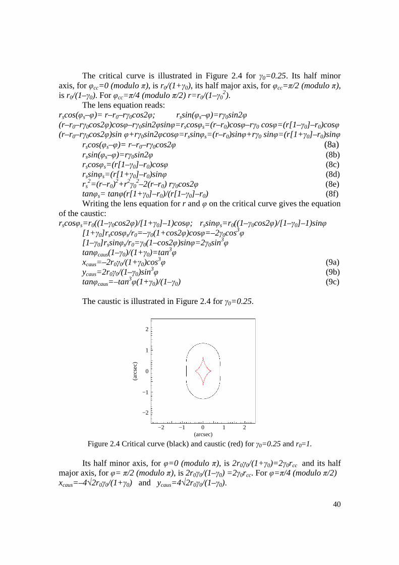
40

The critical curve is illustrated in Figure 2.4 for γ0=0.25. Its half minor axis, for φcc=0 (modulo π), is r0/(1+γ0), its half major axis, for φcc=π /2 (modulo π), is r0/(1–γ0). For φcc=π /4 (modulo π/2) r=r 0/(1–γ0

2). The lens equation reads:

rscos(φs–φ)= r–r 0–rγ0cos2φ; rssin(φs–φ)=rγ 0sin2φ (r–r0–rγ0cos2φ)cosφ–rγ0sin2φsinφ=r scosφs=(r–r 0)cosφ–rγ0 cosφ=(r[1– γ0]–r0)cosφ (r–r0–rγ0cos2φ)sin φ+r γ0sin2φcosφ=r ssinφs=(r–r 0)sinφ+r γ0 sinφ=(r[1+ γ0]–r0)sinφ

rscos(φs–φ)= r–r 0–rγ0cos2φ (8a) rssin(φs–φ)=rγ 0sin2φ (8b) rscosφs=(r[1– γ0]–r 0)cosφ (8c) rssinφs=(r[1+ γ0]–r0)sinφ (8d) rs

2=(r–r 0)2+r 2γ0

2–2(r–r0) rγ0cos2φ (8e) tanφs= tanφ(r[1+ γ0]–r0)/(r[1–γ0]–r0) (8f) Writing the lens equation for r and φ on the critical curve gives the equation

of the caustic: rscosφs=r 0((1–γ0cos2φ)/[1+γ 0]–1)cosφ; rssinφs=r 0((1–γ0cos2φ)/[1–γ0]–1)sinφ

[1+ γ0]r scosφs/r0=–γ0(1+cos2φ)cosφ=–2γ0cos3φ [1–γ0]r ssinφs/r0=γ0(1–cos2φ)sinφ=2γ0sin3φ tanφcaus(1–γ0)/(1+γ0)=tan3φ xcaus=–2r0γ0/(1+γ0)cos3φ (9a) ycaus=2r0γ0/(1–γ0)sin3φ (9b) tanφcaus=–tan3φ(1+γ0)/(1–γ0) (9c) The caustic is illustrated in Figure 2.4 for γ0=0.25.

Figure 2.4 Critical curve (black) and caustic (red) for γ0=0.25 and r0=1.

Its half minor axis, for φ=0 (modulo π), is 2r0γ0/(1+γ0)=2γ0rcc and its half

major axis, for φ= π/2 (modulo π), is 2r0γ0/(1–γ0) =2γ0rcc. For φ=π /4 (modulo π/2) xcaus=–4√2r0γ0/(1+γ0) and ycaus=4√2r0γ0/(1–γ0).

(arc

sec)

−2 −1 0 1 2

2

1

0

−1

−2

(arcsec)

41

Solving the lens equation is conveniently done by eliminating r. Writing r1=(r scosφs+r 0cosφ)/[1–γ0]cosφ (10a) r2=(r ssinφs+r 0sinφ)/[1+ γ0]sinφ (10b) the lens equation reads r1=r 2

(rs cosφs +r 0cosφ)[1+γ 0] sinφ = (rs sinφs +r 0sinφ)[1−γ 0] cosφ rscosφs sinφ [1+ γ0] −sinφs cosφ [1−γ0]= r s sin(φ−φ s) +γ0 sin(φ+φ s)

=−r 0cosφ sinφ [1+ γ0]−sinφ cosφ [1− γ0]= −r 0 γ0 sin2φ f=r s/r0=−γ 0 sin2φ/sin(φ−φ s)+γ0sin(φ+φ s) (11) Hence the procedure for solving the lens equation: one searches for the

zeroes of the function f–rs/r0 meaning for the values of φ where f is equal to rs/r0. The function f is displayed in Figure 2.5 for γ0=0.25. Depending on the value of rs/r0 we see that the equation has two or four solutions. The case rs=0.2 is illustrated in the figure. It gives four solutions because the source is inside the caustic. Also shown in Figure 2.5 are the functions r1 and r2 that have been drawn for rs=0.2. They take equal values whenever φ is a solution of the lens equation. Similarly, we define r3 and r4 as shown below:

rscos(φs–φ)=r(1–γ0cos2φ)–r0 rssin(φs–φ)=rγ 0sin2φ r3=r scos(φs–φ)+r 0/(1–γ0cos2φ) (12a) r4=r ssin(φs–φ)/(γ0sin2φ) (12b) When φ is a root of the lens equation, r1, r2, r3 and r4 are all equal and their

common value is the r of the image. The functions r3 and r4 are also displayed on Figure 2.5.

Figure 2.6 illustrates the case rs=0.4, corresponding to only two images. It is apparent from Figures 2.5 and 2.6 that the lens equation is difficult to

solve precisely when the source crosses the caustic, at the transition between two and four images. In such a case, r1 and r2 are tangent, as are r3 and r4 and f and the line f=r s/r0. The images that disappear stay at nearly constant radius but their angular separation decreases rapidly. The derivative of f with respect to φ cancels precisely at the transition from four to two images when the source crosses the caustic.

2cos2φ sin(φ−φ s) +γ0 sin(φ+φ s)= sin2φ cos(φ−φs) +γ0 cos(φ+φ s) Writing t=tan φ, cs=cosφs and ss=sin φs, 2cs−ss/t+γ0cs+γ0ss/t=2t/(1–t2)cs/t+ss+γ0cs/t−γ0ss (1−t2) cs−ss/t+γ0cs+γ0ss/t=c s+tss+γ0cs−γ0tss (1+ γ0)cst–(1+ γ0)cst

3–ss(1−γ0)+ss(1−γ0)t2=(1+ γ0)cst+ss(1−γ0)t

2 (1+ γ0)cst

3=−ss(1− γ0) tan3φ=−tanφs[1−γ 0]/[1+γ 0] As expected, the polar angle of the image and the polar angle of the source

are related by the caustic equation. The function tan3φ+tanφs[1−γ0]/[1+γ 0] is displayed in Figure 2.7 together with f, r1, r2, r3 and r4 for rs=0.2808, very close to the caustic.

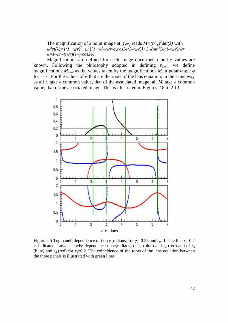
42

The magnification of a point image at (r,φ) reads M=(r/r s)2det(λ) with

µdet(λ)= (1−r0/r)2−γ0

21+ γ02–r0/r–γ0cos2φ(2–r0/r)+2 γ0

2sin22φ(1–r0/r)r 0/r µ=1–γ0

2–(r0/r)(1–γ0cos2φ). Magnifications are defined for each image once their r and φ values are

known. Following the philosophy adopted in defining r1to4, we define magnifications M1to4 as the values taken by the magnifications Mi at polar angle φ for r=r i. For the values of φ that are the roots of the lens equation, in the same way as all r i take a common value, that of the associated image, all Mi take a common value, that of the associated image. This is illustrated in Figures 2.8 to 2.13.

Figure 2.5 Top panel: dependence of f on φ[radians] for γ0=0.25 and r0=1. The line rs=0.2 is indicated. Lower panels: dependence on φ[radians] of r1 (blue) and r2 (red) and of r3 (blue) and r4 (red) for rs=0.2. The coincidence of the roots of the lens equation between the three panels is illustrated with green lines.

φ[radians]

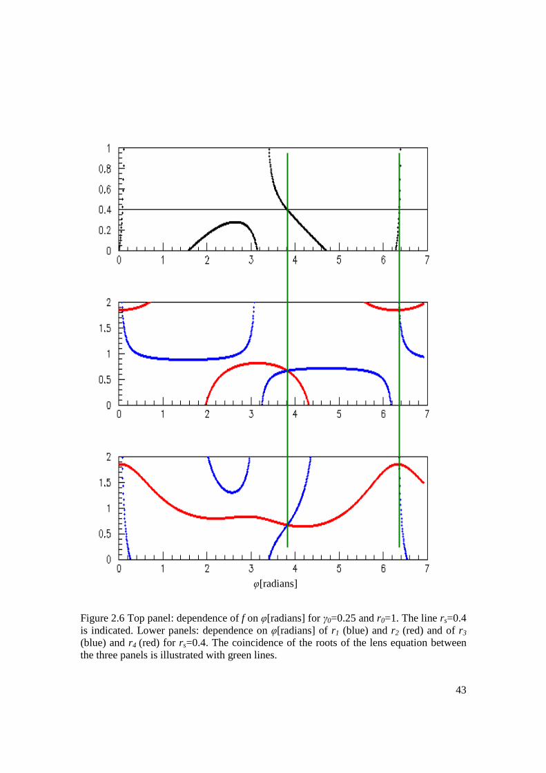
43

Figure 2.6 Top panel: dependence of f on φ[radians] for γ0=0.25 and r0=1. The line rs=0.4 is indicated. Lower panels: dependence on φ[radians] of r1 (blue) and r2 (red) and of r3 (blue) and r4 (red) for rs=0.4. The coincidence of the roots of the lens equation between the three panels is illustrated with green lines.

φ[radians]

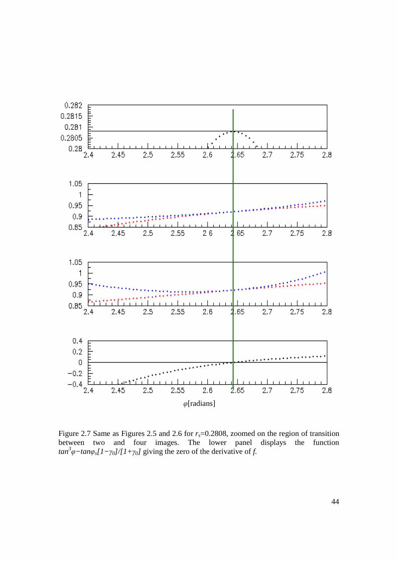
44

Figure 2.7 Same as Figures 2.5 and 2.6 for rs=0.2808, zoomed on the region of transition between two and four images. The lower panel displays the function tan3φ−tanφs[1−γ0]/[1+ γ0] giving the zero of the derivative of f.

φ[radians]

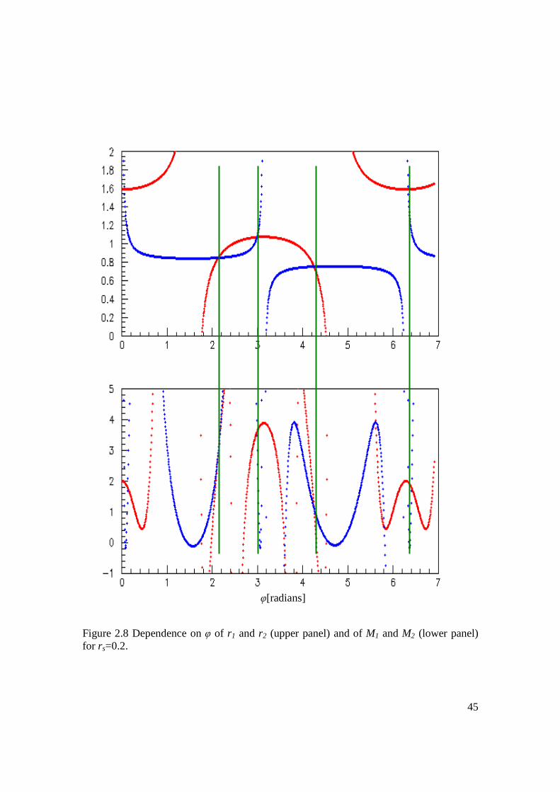
45

Figure 2.8 Dependence on φ of r1 and r2 (upper panel) and of M1 and M2 (lower panel) for rs=0.2.

φ[radians]

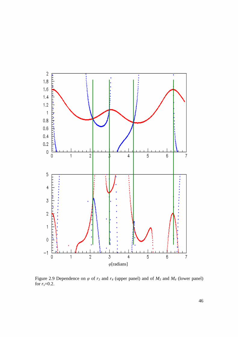
46

Figure 2.9 Dependence on φ of r3 and r4 (upper panel) and of M3 and M4 (lower panel) for rs=0.2.

φ[radians]

47

Figure 2.10 Dependence on φ of r1 and r2 (upper panel) and of M1 and M2 (lower panel) for rs=0.4.

φ[radians]

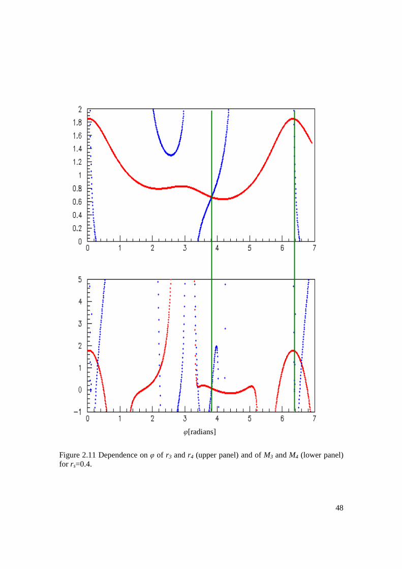
48

Figure 2.11 Dependence on φ of r3 and r4 (upper panel) and of M3 and M4 (lower panel) for rs=0.4.

φ[radians]

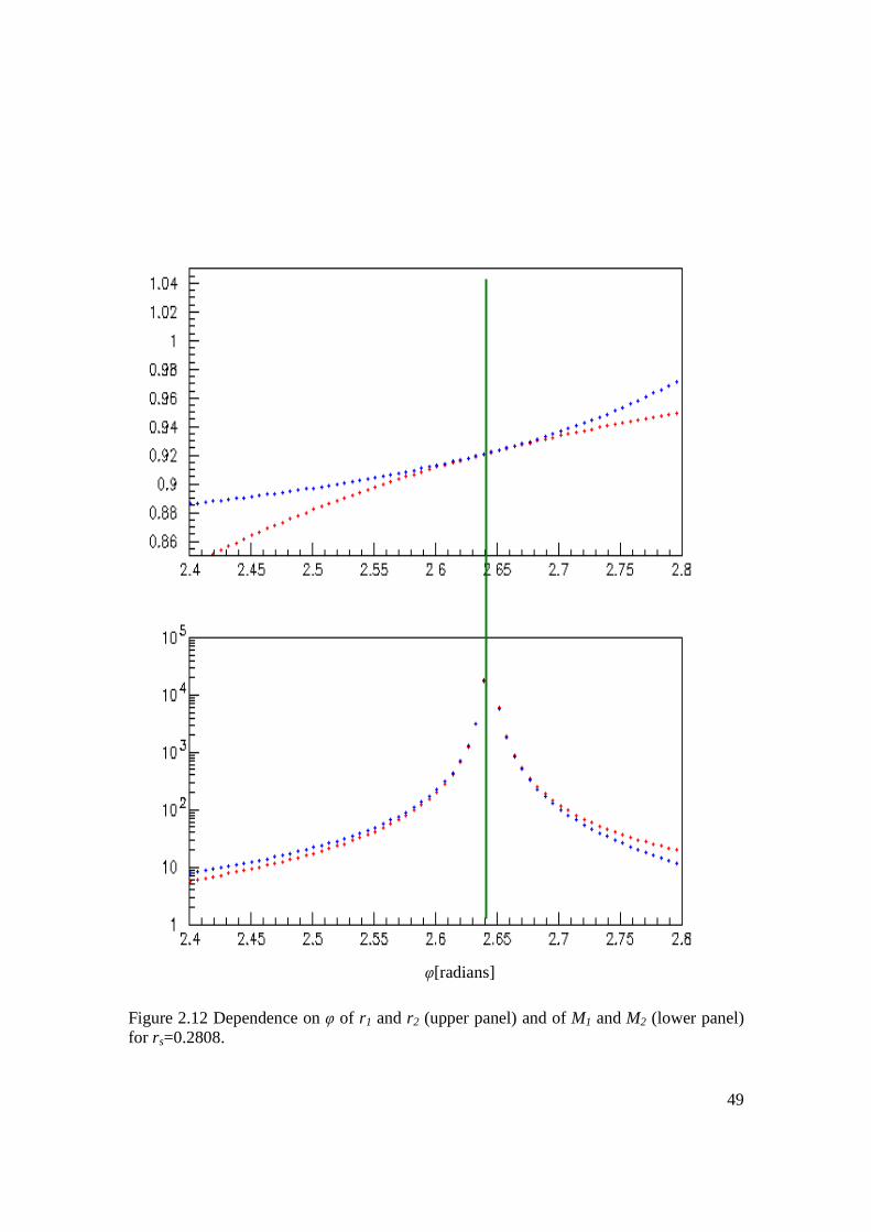
49

Figure 2.12 Dependence on φ of r1 and r2 (upper panel) and of M1 and M2 (lower panel) for rs=0.2808.

φ[radians]

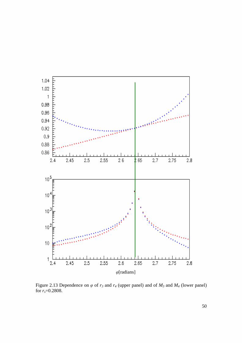
50

Figure 2.13 Dependence on φ of r3 and r4 (upper panel) and of M3 and M4 (lower panel) for rs=0.2808.

φ[radians]

51

2.4 Vicinity of the caustic and critical curve As the host galaxy of RX J0911 overlaps the caustic, we must pay

particular attention to the behaviour of the lens equation when the source approaches the caustic or when an image approaches the critical curve. In order to further illustrate such situations we keep using, in the present section, the same simple potential as in the preceding one.

Figure 2.14 displays the dependence of the magnifications of the two images that disappear when the source is crossing the caustic from inside to outside as a function of rs and φ separately. To draw this figure, we proceed as follows: γ0 being fixed at 0.25 and φs at 15o, we vary φ in steps of 2π/1000 in the interval [2.4, 2.9 radians] where two images are known to disappear. Knowing φ we calculate r=r 1=r 2=r 3=r 4. We then can calculate the magnification M and plot it as a function of rs and of φ. As expected, the images are observed to disappear around rs=0.2808 in the upper panel. Before disappearing the two images associated with a same value of rs have similar magnifications. The lower panel illustrates how the magnifications go to infinity when tan3φ=−tanφs[1−γ 0]/[1+γ 0] , namely at φ=2.64 radians. Again the two images are seen to have similar magnifications for values of φ equally distant from 2.64 radians.

Note that the magnifications exceed ~100 (20) over an rs interval of some 1.6 (8.2) 10–3 r0, implying that in such a region care must be taken to account for their rapid variation.

Figure 2.15 (left) shows the position of the disappearing images together with the critical curve. We see that the last pair of images before disappearance is nearly 0.05 r0 apart while for an increase of rs of only 0.0005r0 the pair disappears. This implies that if we plot the image positions for a grid of source positions having a mesh δ, there will be a no man’s land in the image map around the critical curve, with a width of nearly 100 δ.

Indeed, differentiating the lens equation for constant φs, we get: drscosφs=[1–γ]cosφdr–(r[1–γ]–1)sinφdφ drssinφs=[1+γ ]sinφdr+(r[1+ γ]–1)cosφdφ [1+γ ]sinφcosφs–[1–γ]cosφsinφsdrs

=–(r[1– γ]–1)sin2φ[1+ γ]–(r[1+ γ]–1)cos2φ[1–γ] dφ sin(φ–φs)+γsin(φ+φ s)drs=1–r(1–γ2) –γcos2φ dφ=(1–γ2)(rcc–r) dφ dφ/drs=sin(φ–φs)+γsin(φ+φ s)/(1–γ2)(rcc–r) Similarly, dr/drs=(r–1)cos(φ–φs)+rγ cos(φ+φ s)/(r–r cc)(1–γ2) Writing the pair size as D=(dr2+rdφ2)1/2, dD/drs=∆½(1–γ2)–1|rcc–r|–1 with ∆=r 2(1+γ2+2γcos2φs)–2rcos(φ–φs)[1+ γcos(φ+φ s)]+cos2(φ–φs)

½ The derivatives of the coordinates of the image with respect to rs at constant

φs diverge near the critical curve as |rcc–r|–1.

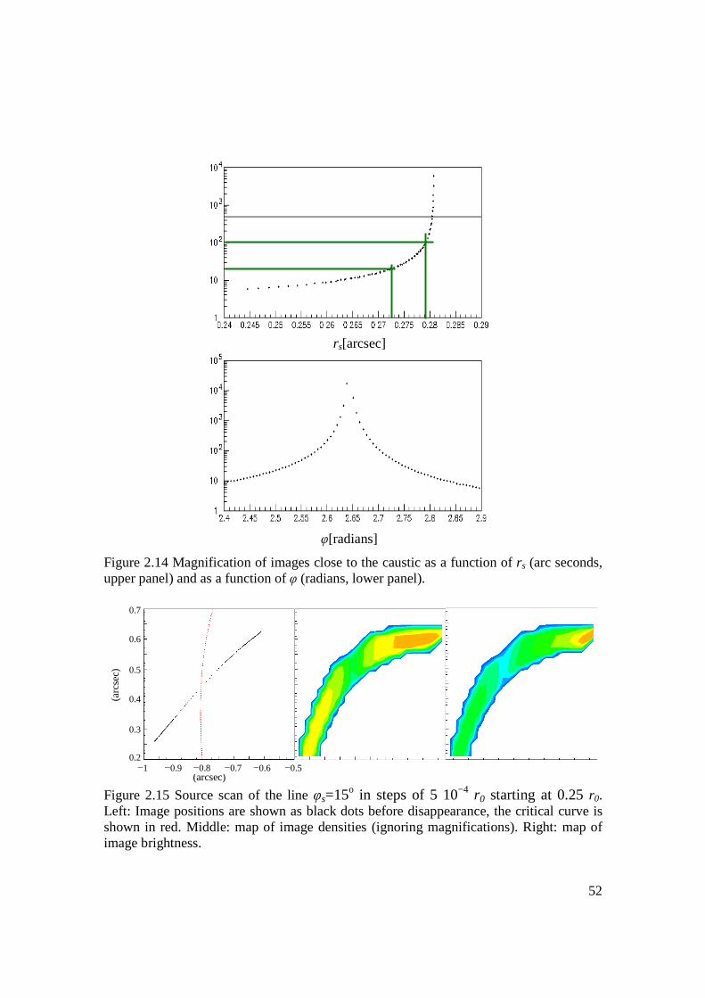
52

Figure 2.14 Magnification of images close to the caustic as a function of rs (arc seconds, upper panel) and as a function of φ (radians, lower panel).

Figure 2.15 Source scan of the line φs=15o in steps of 5 10−4 r0 starting at 0.25 r0. Left: Image positions are shown as black dots before disappearance, the critical curve is shown in red. Middle: map of image densities (ignoring magnifications). Right: map of image brightness.

(arcsec)

0.7

0.6

0.5

0.4

0.3

0.2−1 −0.9 −0.8 −0.7 −0.6 −0.5

(arc

sec)

φ[radians]

rs[arcsec]

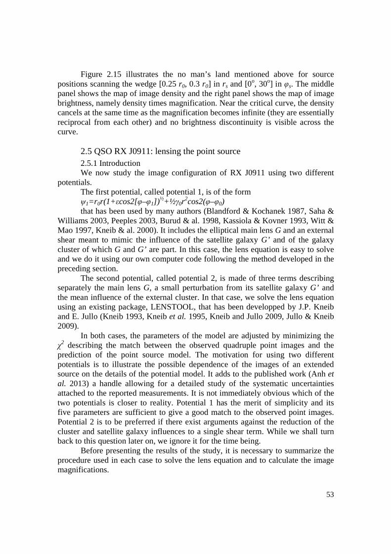
53

Figure 2.15 illustrates the no man’s land mentioned above for source positions scanning the wedge [0.25 r0, 0.3 r0] in rs and [0o, 30o] in φs. The middle panel shows the map of image density and the right panel shows the map of image brightness, namely density times magnification. Near the critical curve, the density cancels at the same time as the magnification becomes infinite (they are essentially reciprocal from each other) and no brightness discontinuity is visible across the curve.

2.5 QSO RX J0911: lensing the point source 2.5.1 Introduction We now study the image configuration of RX J0911 using two different

potentials. The first potential, called potential 1, is of the form ψ1=r 0r(1+εcos2[φ–φ1])

½+½γ0r2cos2(φ–φ0)

that has been used by many authors (Blandford & Kochanek 1987, Saha & Williams 2003, Peeples 2003, Burud & al. 1998, Kassiola & Kovner 1993, Witt & Mao 1997, Kneib & al. 2000). It includes the elliptical main lens G and an external shear meant to mimic the influence of the satellite galaxy G’ and of the galaxy cluster of which G and G’ are part. In this case, the lens equation is easy to solve and we do it using our own computer code following the method developed in the preceding section.

The second potential, called potential 2, is made of three terms describing separately the main lens G, a small perturbation from its satellite galaxy G’ and the mean influence of the external cluster. In that case, we solve the lens equation using an existing package, LENSTOOL, that has been developped by J.P. Kneib and E. Jullo (Kneib 1993, Kneib et al. 1995, Kneib and Jullo 2009, Jullo & Kneib 2009).

In both cases, the parameters of the model are adjusted by minimizing the χ2 describing the match between the observed quadruple point images and the prediction of the point source model. The motivation for using two different potentials is to illustrate the possible dependence of the images of an extended source on the details of the potential model. It adds to the published work (Anh et al. 2013) a handle allowing for a detailed study of the systematic uncertainties attached to the reported measurements. It is not immediately obvious which of the two potentials is closer to reality. Potential 1 has the merit of simplicity and its five parameters are sufficient to give a good match to the observed point images. Potential 2 is to be preferred if there exist arguments against the reduction of the cluster and satellite galaxy influences to a single shear term. While we shall turn back to this question later on, we ignore it for the time being.

Before presenting the results of the study, it is necessary to summarize the procedure used in each case to solve the lens equation and to calculate the image magnifications.

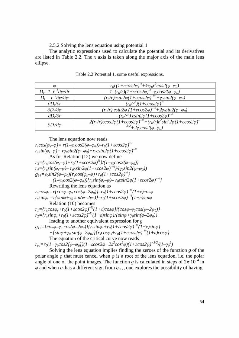
54

2.5.2 Solving the lens equation using potential 1 The analytic expressions used to calculate the potential and its derivatives

are listed in Table 2.2. The x axis is taken along the major axis of the main lens ellipse.

Table 2.2 Potential 1, some useful expressions.

ψ r0r(1+εcos2φ)½+½γ0r

2cos2(φ–φ0) Dr=1–r–1∂ψ/∂r 1–(r0/r)(1+εcos2φ)½–γ0cos2(φ–φ0) Di=–r–2∂ψ/∂φ (r0/r)εsin2φ(1+εcos2φ)–½ +γ0sin2(φ–φ0)

∂Dr/∂r (r0/r2)(1+εcos2φ)½

∂Dr/∂φ (r0/r) εsin2φ (1+εcos2φ)–½+2γ0sin2(φ–φ0) ∂Di/∂r –(r0/r

2) εsin2φ(1+εcos2φ)–½

∂Di/∂φ 2(r0/r)εcos2φ(1+εcos2φ)–½+(r0/r)ε

2sin22φ(1+εcos2φ)–

3/2+2γ0cos2(φ–φ0) The lens equation now reads

rscos(φs–φ)= r(1–γ0cos2(φ–φ0))–r0(1+εcos2φ)½ rssin(φs–φ)= r γ0sin2(φ–φ0)+r 0εsin2φ(1+εcos2φ)–½

As for Relation (12) we now define r3=r scos(φs–φ)+r 0(1+εcos2φ)½/(1–γ0cos2(φ–φ0)) r4=r ssin(φs–φ)– r0εsin2φ(1+εcos2φ)–½/(γ0sin2(φ–φ0)) g34=γ0sin2(φ–φ0)r scos(φs–φ)+r 0(1+εcos2φ)½

−(1–γ0cos2(φ–φ0))r ssin(φs–φ)– r0εsin2φ(1+εcos2φ)–½ Rewriting the lens equation as

rscosφs=rcosφ–γ0 cos(φ–2φ0)–r0(1+εcos2φ)–½(1+ε)cosφ rssinφs =rsinφ+γ0 sin(φ–2φ0)–r0(1+εcos2φ)–½(1−ε)sinφ

Relation (10) becomes r1=r scosφs+r 0(1+εcos2φ)–½(1+ε)cosφ/cosφ–γ0cos(φ–2φ0) r2=r ssinφs+r 0(1+εcos2φ)–½(1−ε)sinφ/sinφ+γ0sin(φ–2φ0)

leading to another equivalent expression for g g12=cosφ–γ0 cos(φ–2φ0)r ssinφs+r 0(1+εcos2φ)–½(1−ε)sinφ

−sinφ+γ0 sin(φ–2φ0)r scosφs+r 0(1+εcos2φ)–½(1+ε)cosφ The equation of the critical curve now reads rcc=r 0(1−γ0cos2[φ–φ0])(1− εcos2φ−2ε2cos2φ)(1+εcos2φ)−3/2/(1–γ0

2) Solving the lens equation implies finding the zeroes of the function g of the

polar angle φ that must cancel when φ is a root of the lens equation, i.e. the polar angle of one of the point images. The function g is calculated in steps of 2π 10–4 in φ and when gi has a different sign from gi+1, one explores the possibility of having

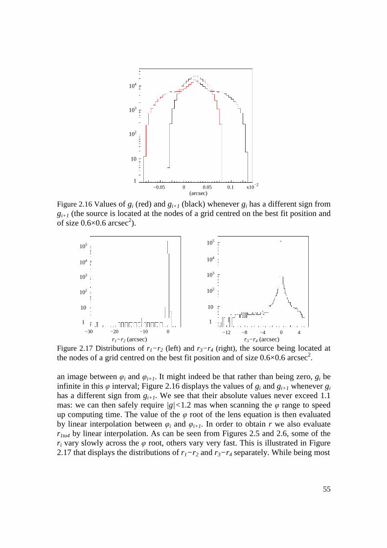
55

(arcsec)

Figure 2.16 Values of gi (red) and gi+1 (black) whenever gi has a different sign from gi+1 (the source is located at the nodes of a grid centred on the best fit position and of size 0.6×0.6 arcsec2).

Figure 2.17 Distributions of r1−r 2 (left) and r3−r 4 (right), the source being located at the nodes of a grid centred on the best fit position and of size 0.6×0.6 arcsec2.

an image between φi and φi+1. It might indeed be that rather than being zero, gi be infinite in this φ interval; Figure 2.16 displays the values of gi and gi+1 whenever gi has a different sign from gi+1. We see that their absolute values never exceed 1.1 mas: we can then safely require |g|<1.2 mas when scanning the φ range to speed up computing time. The value of the φ root of the lens equation is then evaluated by linear interpolation between φi and φi+1. In order to obtain r we also evaluate r1to4 by linear interpolation. As can be seen from Figures 2.5 and 2.6, some of the r i vary slowly across the φ root, others vary very fast. This is illustrated in Figure 2.17 that displays the distributions of r1−r 2 and r3−r 4 separately. While being most

104

103

102

10

1−0.05 0 0.05 0.1 x10

−2

105

104

103

102

10

1

−30 −20 −10 0 −12 −8 −4 0 4

r1−r2 (arcsec) r3−r4 (arcsec)

105

104

103

102

10

1

56

of the time quite small, both have large tails. However, as displayed in Figure 2.18, the smaller of |r1−r 2| and |r3−r 4| is always very small and never exceeds 8 mas. Therefore, we first look for which of the (1,2) and (3,4) pairs gives the smaller difference and we take for r the mean of the corresponding r values: (r1+r 2)/2 if |r1−r 2|<|r 3−r 4| and (r3+r 4)/2 if |r1−r 2|>|r 3−r 4|. The results of the best fit to the HST images are listed in Tables 2.3 and 2.4 and illustrated in Figure 2.19. The χ2 is simply the sum over the four images of the products Mmodelδ

2 where δ stands for the distance between the observed and predicted point images. Namely, a constant measurement error has been assumed. Figure 2.20 displays the χ2 map in the source plane in the neighbourhood of the best fit result.

Figure 2.18 Distribution of |r1−r 2| when |r1−r 2| is smaller than |r3−r 4| (black) and of |r3−r 4| when |r3−r 4| is smaller than |r1−r 2| (red). The source is located at the nodes of a grid centred on the best fit position and of size 0.6×0.6 arcsec2.

Table 2.3

Best fit results (r in arcseconds and φ in degrees)

A1 A2 A3 B robs 0.866 0.964 0.814 2.291

rmodel (ψ1) 0.850 0.967 0.821 2.258 φobs 216.3 186.3 146.6 7.0

φmodel (ψ1) 219.2 187.6 150.6 5.8 M (ψ1) –4.07 8.05 –3.52 1.76

(arcsec)

104

103

102

10

1

−1 0 1 2 3 4 5 6 7 8 x10 −3

(arcsec)

57

Table 2.4

Best fit values of the parameters (angles in degrees and angular distances in arcseconds)

Potential ψ1 r0 ε φ1 γ0 φ0 rs φs

1.1085 −0.0237 65.0 0.309 7.32 0.4468 4.18

Figure 2.19 Left: Image positions obtained using potential 1 are shown as blue crosses for a point source (blue asterisk). The lens G is at the origin of coordinates (black circle). Red crosses indicate the HST observed image positions. Right: map of images (red for 4-images and blue for 2-images) obtained for point sources at the nodes of a grid of 0.6”×0.6” centred on the best fit source position (mesh size of 2 mas). The no man’s land on either sides of the critical curve is clearly seen. The critical curve is shown on both panels.

Figure 2.20 Contours in the source plane of the χ2 distribution of the match between the HST images and the potential 1 prediction. Axes are labelled in arcseconds, the colour scale is in log(χ2) up to an additional constant.

2

1

0

−1

−2

−1 0 1 2 3 −1 0 1 2 3

2

1

0

−1

−2

(arcsec) (arcsec)

(a

rcse

c)

(a

rcse

c)

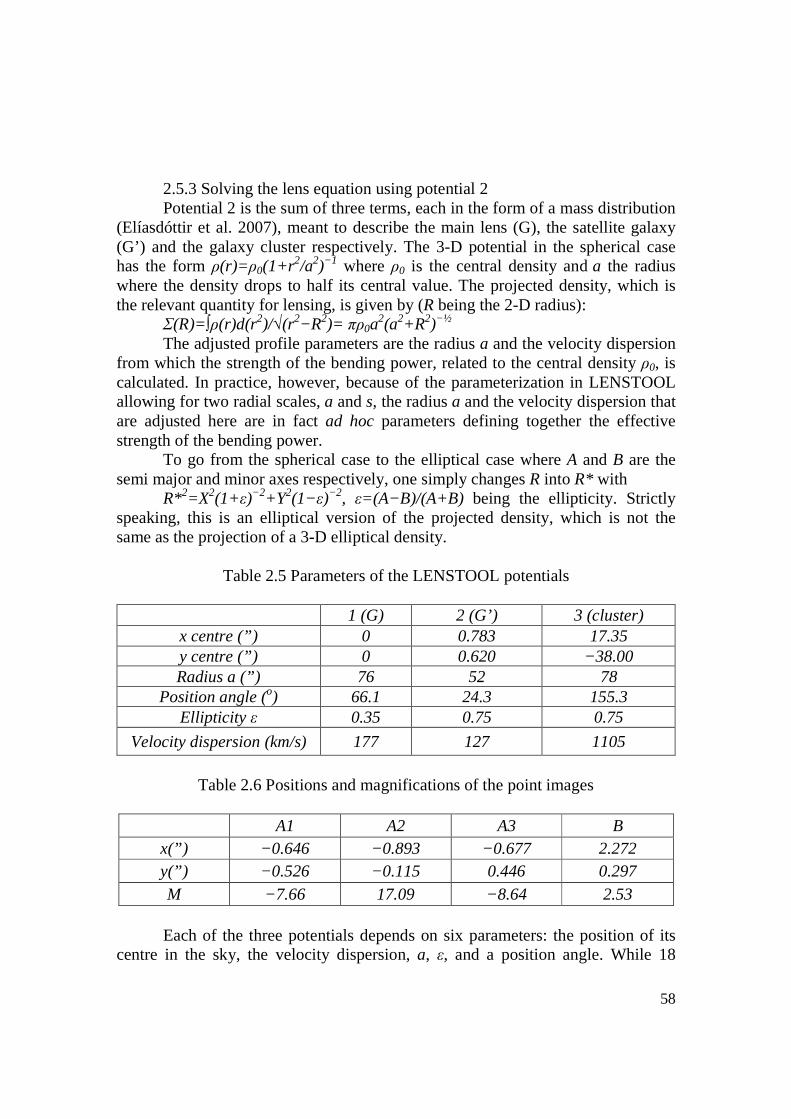
58

2.5.3 Solving the lens equation using potential 2 Potential 2 is the sum of three terms, each in the form of a mass distribution

(Elíasdóttir et al. 2007), meant to describe the main lens (G), the satellite galaxy (G’) and the galaxy cluster respectively. The 3-D potential in the spherical case has the form ρ(r)= ρ0(1+r2/a2)−1 where ρ0 is the central density and a the radius where the density drops to half its central value. The projected density, which is the relevant quantity for lensing, is given by (R being the 2-D radius):

Σ(R)=∫ρ(r)d(r2)/√(r2−R2)= πρ0a2(a2+R2)−½

The adjusted profile parameters are the radius a and the velocity dispersion from which the strength of the bending power, related to the central density ρ0, is calculated. In practice, however, because of the parameterization in LENSTOOL allowing for two radial scales, a and s, the radius a and the velocity dispersion that are adjusted here are in fact ad hoc parameters defining together the effective strength of the bending power.

To go from the spherical case to the elliptical case where A and B are the semi major and minor axes respectively, one simply changes R into R* with

R*2=X2(1+ε)−2+Y2(1−ε)−2, ε=(A−B)/(A+B) being the ellipticity. Strictly speaking, this is an elliptical version of the projected density, which is not the same as the projection of a 3-D elliptical density.

Table 2.5 Parameters of the LENSTOOL potentials

1 (G) 2 (G’) 3 (cluster)

x centre (”) 0 0.783 17.35 y centre (”) 0 0.620 −38.00 Radius a (”) 76 52 78

Position angle (o) 66.1 24.3 155.3 Ellipticity ε 0.35 0.75 0.75

Velocity dispersion (km/s) 177 127 1105

Table 2.6 Positions and magnifications of the point images

A1 A2 A3 B

x(”) −0.646 −0.893 −0.677 2.272 y(”) −0.526 −0.115 0.446 0.297

M −7.66 17.09 −8.64 2.53 Each of the three potentials depends on six parameters: the position of its

centre in the sky, the velocity dispersion, a, ε, and a position angle. While 18

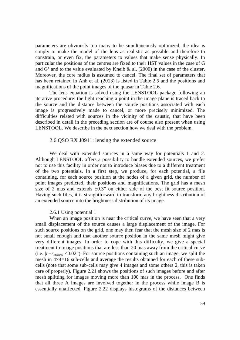
59

parameters are obviously too many to be simultaneously optimized, the idea is simply to make the model of the lens as realistic as possible and therefore to constrain, or even fix, the parameters to values that make sense physically. In particular the positions of the centres are fixed to their HST values in the case of G and G’ and to the value evaluated by Kneib & al. (2000) in the case of the cluster. Moreover, the core radius is assumed to cancel. The final set of parameters that has been retained in Anh et al. (2013) is listed in Table 2.5 and the positions and magnifications of the point images of the quasar in Table 2.6.

The lens equation is solved using the LENSTOOL package following an iterative procedure: the light reaching a point in the image plane is traced back to the source and the distance between the source positions associated with each image is progressively made to cancel, or more precisely minimized. The difficulties related with sources in the vicinity of the caustic, that have been described in detail in the preceding section are of course also present when using LENSTOOL. We describe in the next section how we deal with the problem.

2.6 QSO RX J0911: lensing the extended source

We deal with extended sources in a same way for potentials 1 and 2.

Although LENSTOOL offers a possibility to handle extended sources, we prefer not to use this facility in order not to introduce biases due to a different treatment of the two potentials. In a first step, we produce, for each potential, a file containing, for each source position at the nodes of a given grid, the number of point images predicted, their positions and magnifications. The grid has a mesh size of 2 mas and extends ±0.3” on either side of the best fit source position. Having such files, it is straightforward to transform any brightness distribution of an extended source into the brightness distribution of its image.

2.6.1 Using potential 1 When an image position is near the critical curve, we have seen that a very

small displacement of the source causes a large displacement of the image. For such source positions on the grid, one may then fear that the mesh size of 2 mas is not small enough and that another source position in the same mesh might give very different images. In order to cope with this difficulty, we give a special treatment to image positions that are less than 20 mas away from the critical curve (i.e. |r−r critical|<0.02”). For source positions containing such an image, we split the mesh in 4×4=16 sub-cells and average the results obtained for each of these sub-cells (note that some sub-cells may give 4 images and some others 2, this is taken care of properly). Figure 2.21 shows the positions of such images before and after mesh splitting for images moving more than 100 mas in the process. One finds that all three A images are involved together in the process while image B is essentially unaffected. Figure 2.22 displays histograms of the distances between

60

old and new image positions for all grid nodes having received the special treatment. Here again, we see how very small source displacements are causing large displacements of the A images in such cases (image B moves by less than 1 mas). Figure 2.23 displays histograms of the differences in magnification between old and new image positions for all nodes having received the special treatment.

Figure 2.21 Positions of images for source positions on the grid nodes such that at least one image is less than 20 mas away from the critical curve. Only images moving by more than 100 mas in the cell splitting process are displayed. Their positions are shown before cell-splitting (left panel) and after cell-splitting (right panel).

Figure 2.22 Histograms of the distances by which images move in the cell-splitting process (from left to right, A1, A2, A3 and B). Full scale is 0.8” for images A and 1.5 mas for B.

In view of the above results, we decide to apply the special treatment to all source positions giving at least one image distant by less than 50 mas (rather than 20 mas) from the critical curve. Moreover, rather than taking unweighted position averages, as was done, we take position averages weighted by the associated

10

1

10

1

10

1

10

1

0 0.2 0.4 0.6 0.8 0 0.2 0.4 0.6 0.8 0 0.2 0.4 0.6 0.8 0 0.04 0.08 0.12

(arcsec) (arcsec) (arcsec) (arcsec) x10−2

0.8

0.4

0

−0.4

−0.8

(arcsec)

(a

rcse

c)

−1.2 −0.8 −0.4 0 0.4

61

magnifications. We then draw the equivalents of Figure 2.21 for images moving by more than 20 mas rather than 100 mas. The result is displayed in Figures 2.24.

Figure 2.23 Histograms of the differences in magnifications in the cell-splitting process (from left to right, A1, A2, A3 and B). Scales are −25 to 75 for A1 and A3, −70 to 45 for A2 and −0.01 to 0.01 for B.

Figure 2.24 Positions of images (using potential 1) for source positions on the grid nodes such that at least one image is less than 50 mas away from the critical curve. Only images moving by more than 20 mas in the cell splitting process are displayed. Their positions are shown before cell-splitting (left panel) and after cell-splitting (right panel).

2.6.2 Using potential 2 In the case of potential 2, we noted two trivial problems that needed to be

taken care of. One is the presence in most cases of an additional (direct) image with very low magnification: we simply ignore it. The other is that the program is not protected when setting the core radii to zero exactly (Jullo, E., private communication), which we overcome by simply fixing all core radii to 1 mas. The distribution of the number of images is displayed in Figure 2.25 before and after having fixed these problems. We are then left with 54 cases of 3 images, 8 cases of

102

10

1

10

1

10

1

10

1

−60 −40 −20 0 20 40 −20 0 20 40 60 −0.8 −0.4 0 0.4 0.8 −20 0 20 40 60 x 10−2

0.4

0

−0.4

−0.8

(arcsec)

(a

rcse

c)

−1.2 −0.8 −0.4 0

62

5 images and 2 cases of 6 images; the positions of the source associated with these 64 problematic cases are displayed in Figure 2.26: most of them are near the caustic, only three of them being in the direction of G’. The number of problematic cases is very small, 64/90000~7 10−4; however, they affect precisely source positions relevant to the case of the host galaxy of RX J0911 and deserve therefore to be taken seriously.

Figure 2.25 Distribution of the number of images produced by LENSTOOL before (left) and after (right) ignoring the additional low magnification image and setting core radii.

Figure 2.26 Positions of the sources associated with LENSTOOL producing either 3 (red) or 5 (blue) images. The caustic is drawn to guide the eye. Near the north-west corner of the figure, three source positions are associated with a duplicated image.

(arcsec)

(ar

csec

)

number images number images

105

104

103

102

10

1

105

104

103

102

10

10 2 4 6 8 10 12 0 2 4 6 8 10 12

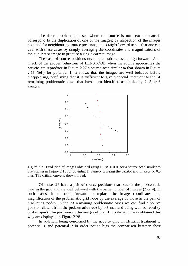
63

The three problematic cases where the source is not near the caustic correspond to the duplication of one of the images; by inspection of the images obtained for neighbouring source positions, it is straightforward to see that one can deal with these cases by simply averaging the coordinates and magnifications of the duplicated image to produce a single correct image.

The case of source positions near the caustic is less straightforward. As a check of the proper behaviour of LENSTOOL when the source approaches the caustic, we reproduce in Figure 2.27 a source scan similar to that shown in Figure 2.15 (left) for potential 1. It shows that the images are well behaved before disappearing, confirming that it is sufficient to give a special treatment to the 61 remaining problematic cases that have been identified as producing 2, 5 or 6 images.

Figure 2.27 Evolution of images obtained using LENSTOOL for a source scan similar to that shown in Figure 2.15 for potential 1, namely crossing the caustic and in steps of 0.5 mas. The critical curve is shown in red.

Of these, 28 have a pair of source positions that bracket the problematic

case in the grid and are well behaved with the same number of images (2 or 4). In such cases, it is straightforward to replace the image coordinates and magnification of the problematic grid node by the average of those in the pair of bracketing nodes. In the 33 remaining problematic cases we can find a source position distant from the problematic node by 0.5 mas and being well behaved (2 or 4 images). The positions of the images of the 61 problematic cases obtained this way are displayed in Figure 2.28.

In addition, being concerned by the need to give an identical treatment to potential 1 and potential 2 in order not to bias the comparison between their

(arcsec)

(a

rcse

c)

0

−0.1

−0.2

−0.3

−0.4

−0.5

−0.6

−0.7

−0.8−1 −0.9 −0.8 −0.7 −0.6

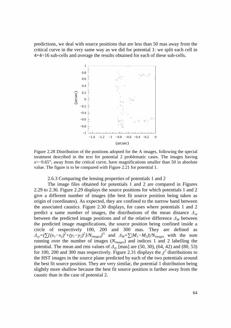
64

predictions, we deal with source positions that are less than 50 mas away from the critical curve in the very same way as we did for potential 1: we split each cell in 4×4=16 sub-cells and average the results obtained for each of these sub-cells.

Figure 2.28 Distribution of the positions adopted for the A images, following the special treatment described in the text for potential 2 problematic cases. The images having x>−0.65”, away from the critical curve, have magnifications smaller than 50 in absolute value. The figure is to be compared with Figure 2.21 for potential 1.

2.6.3 Comparing the lensing properties of potentials 1 and 2 The image files obtained for potentials 1 and 2 are compared in Figures

2.29 to 2.36. Figure 2.29 displays the source positions for which potentials 1 and 2 give a different number of images (the best fit source position being taken as origin of coordinates). As expected, they are confined to the narrow band between the associated caustics. Figure 2.30 displays, for cases where potentials 1 and 2 predict a same number of images, the distributions of the mean distance ∆xy between the predicted image positions and of the relative difference ∆M between the predicted image magnifications, the source position being confined inside a circle of respectively 100, 200 and 300 mas. They are defined as ∆xy=(∑(x1−x2)

2+(y1−y2)2/Nimages)

½ and ∆M=∑|M1−M2)|/Nimages with the sum running over the number of images (Nimages) and indices 1 and 2 labelling the potential. The mean and rms values of ∆xy [mas] are (50, 30), (64, 42) and (80, 53) for 100, 200 and 300 mas respectively. Figure 2.31 displays the χ2 distributions to the HST images in the source plane predicted by each of the two potentials around the best fit source position. They are very similar, the potential 1 distribution being slightly more shallow because the best fit source position is farther away from the caustic than in the case of potential 2.

(arcsec)

(a

rcse

c)

1

0.8

0.6

0.4

0.2

0

−0.2

−0.4

−0.6

−0.8

−1−1.4 −1.2 −1 −0.8 −0.6 −0.4 −0.2 0

65

Figure 2.29 Source positions (shaded light blue) for which potentials 1 and 2 produce a different number of images (one of them producing 2 images and the other producing 4 images). The potential 1 (green) and 2 (red) caustics are also shown.

Figure 2.30 Distributions of the mean distance ∆xy between the predicted image positions (left panel) and of the decimal logarithm of the difference ∆M between the predicted image magnifications (right panel), the source position being confined inside a circle of respectively 100 mas (black), 200 mas (red) and 300 mas (blue) mas.

(arcsec)

(arc

sec)

∆xy (arcsec) ∆M

104

103

102

10

1−3 −2 −1 0 1 2 3

104

103

102

10

0 0.05 0.1 0.15 0.2 0.25 0.3

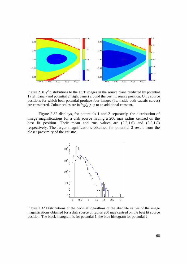
66

Figure 2.31 χ2 distributions to the HST images in the source plane predicted by potential 1 (left panel) and potential 2 (right panel) around the best fit source position. Only source positions for which both potential produce four images (i.e. inside both caustic curves) are considered. Colour scales are in log(χ2) up to an additional constant.

Figure 2.32 displays, for potentials 1 and 2 separately, the distribution of image magnifications for a disk source having a 200 mas radius centred on the best fit position. Their mean and rms values are (2.2,1.6) and (3.5,1.8) respectively. The larger magnifications obtained for potential 2 result from the closer proximity of the caustic.

Figure 2.32 Distributions of the decimal logarithms of the absolute values of the image magnifications obtained for a disk source of radius 200 mas centred on the best fit source position. The black histogram is for potential 1, the blue histogram for potential 2.

104

103

102

10

1

0 0.5 1 1.5 2 2.5 3

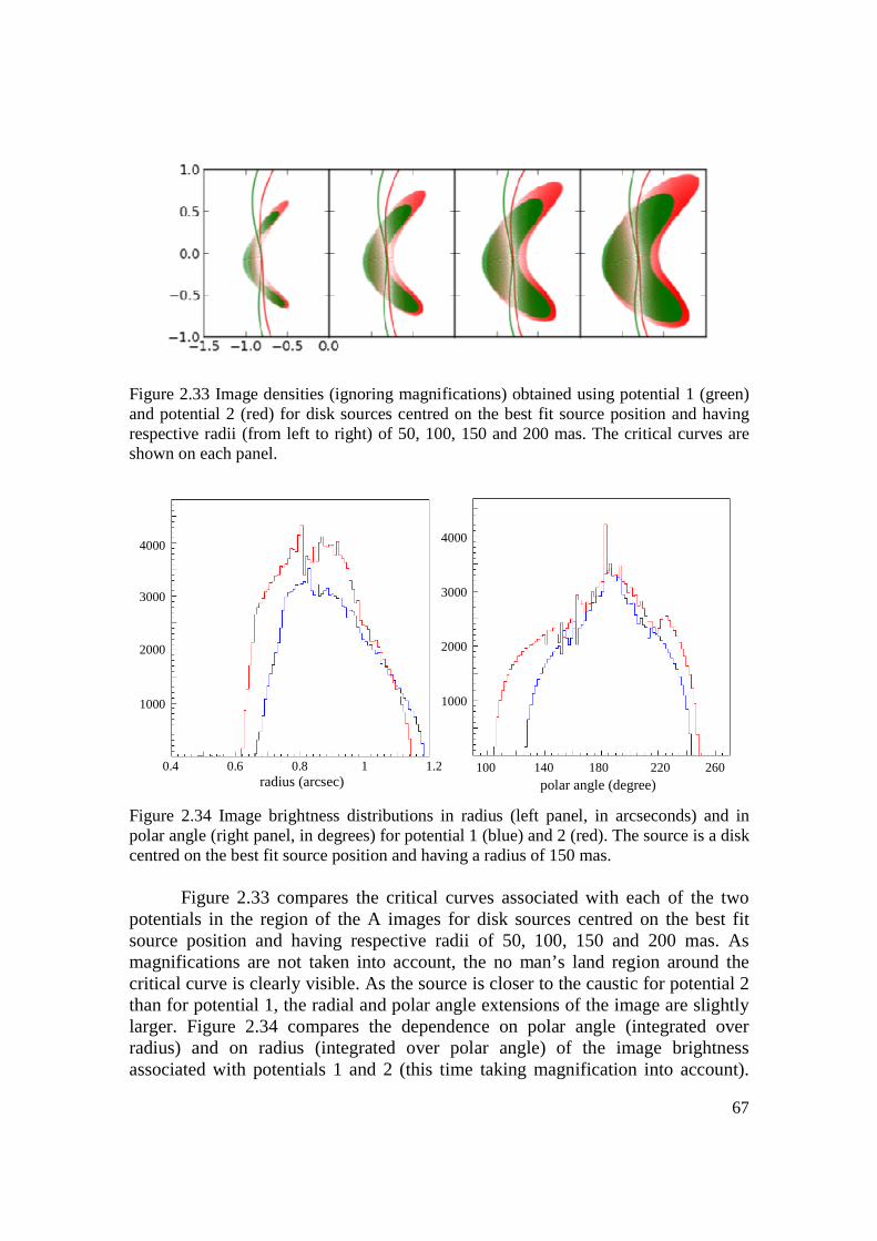
67

Figure 2.33 Image densities (ignoring magnifications) obtained using potential 1 (green) and potential 2 (red) for disk sources centred on the best fit source position and having respective radii (from left to right) of 50, 100, 150 and 200 mas. The critical curves are shown on each panel.

Figure 2.34 Image brightness distributions in radius (left panel, in arcseconds) and in polar angle (right panel, in degrees) for potential 1 (blue) and 2 (red). The source is a disk centred on the best fit source position and having a radius of 150 mas.

Figure 2.33 compares the critical curves associated with each of the two

potentials in the region of the A images for disk sources centred on the best fit source position and having respective radii of 50, 100, 150 and 200 mas. As magnifications are not taken into account, the no man’s land region around the critical curve is clearly visible. As the source is closer to the caustic for potential 2 than for potential 1, the radial and polar angle extensions of the image are slightly larger. Figure 2.34 compares the dependence on polar angle (integrated over radius) and on radius (integrated over polar angle) of the image brightness associated with potentials 1 and 2 (this time taking magnification into account).

radius (arcsec) polar angle (degree)

4000

3000

2000

1000

4000

3000

2000

1000

0.4 0.6 0.8 1 1.2 100 140 180 220 260

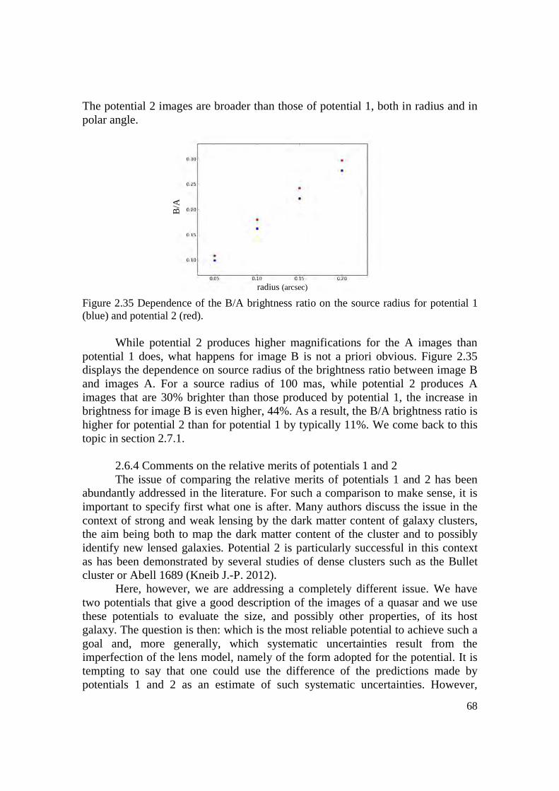
68

The potential 2 images are broader than those of potential 1, both in radius and in polar angle.

Figure 2.35 Dependence of the B/A brightness ratio on the source radius for potential 1 (blue) and potential 2 (red).

While potential 2 produces higher magnifications for the A images than potential 1 does, what happens for image B is not a priori obvious. Figure 2.35 displays the dependence on source radius of the brightness ratio between image B and images A. For a source radius of 100 mas, while potential 2 produces A images that are 30% brighter than those produced by potential 1, the increase in brightness for image B is even higher, 44%. As a result, the B/A brightness ratio is higher for potential 2 than for potential 1 by typically 11%. We come back to this topic in section 2.7.1.

2.6.4 Comments on the relative merits of potentials 1 and 2 The issue of comparing the relative merits of potentials 1 and 2 has been abundantly addressed in the literature. For such a comparison to make sense, it is important to specify first what one is after. Many authors discuss the issue in the context of strong and weak lensing by the dark matter content of galaxy clusters, the aim being both to map the dark matter content of the cluster and to possibly identify new lensed galaxies. Potential 2 is particularly successful in this context as has been demonstrated by several studies of dense clusters such as the Bullet cluster or Abell 1689 (Kneib J.-P. 2012). Here, however, we are addressing a completely different issue. We have two potentials that give a good description of the images of a quasar and we use these potentials to evaluate the size, and possibly other properties, of its host galaxy. The question is then: which is the most reliable potential to achieve such a goal and, more generally, which systematic uncertainties result from the imperfection of the lens model, namely of the form adopted for the potential. It is tempting to say that one could use the difference of the predictions made by potentials 1 and 2 as an estimate of such systematic uncertainties. However,

radius (arcsec)

B/A

69

strictly speaking, this is not justified: it might be that one potential gives a much better model than the other; or it might be that they both give similar results but that the physics reality is quite different.

Potential 2 has a stronger physics basis than potential 1: the existence of an important dark matter halo in the galaxy cluster is well established (Kneib, J.-P. et al., 2000) and its modelling using potential 2 has been shown to be sensible; moreover, accounting for the presence of the satellite galaxy G’ has been shown by Schechter (2005) to change the predicted time delay by 10%. Yet, from the quality of the fit obtained on the quasar images, potential 1 gives a better fit than potential 2. As commented earlier by Saha & Williams (2003), the precise position of the point images, including the strong asymmetry between the A and B images, severely constrains the position of the source with respect to the caustic cusp, with little dependence on the precise form of the effective potential. One might then argue that in the particular case of the host galaxy of RX J0911 overlapping the lens caustic, the details of the potential are of little relevance.

To summarize, we are unable to state with confidence that one potential is more reliable than the other in the particular case that is under study here and we shall continue to use both potentials 1 and potential 2 on an equal footing. While we are hoping that the difference between their predictions gives a reasonable estimate of the systematic uncertainties attached to the imperfection of the lens model, we are also aware that we have no proof that this is indeed the case.

2.7 Additional comments 2.7.1 B/A brightness ratio The relative occurrence of two-image configurations increases with the size

of the source, causing the A images to become globally fainter with respect to image B, the latter being always present in the two-image configuration. This suggests using the apparent brightness ratio B/A as a measure of the source size. This ratio is essentially unaffected by beam convolution and its measurement does not require a very good angular resolution (yet sufficient to separate A from B). However, as image B is not much magnified, it requires a high sensitivity to be obtained with good precision.

To understand what happens, it is essential to keep in mind that magnifications depend strongly on the position of the source point with respect to the caustic cusp, or equivalently on the position of the image point with respect to the critical curve. This is illustrated in Figure 2.36, which displays separately the variations over the source plane of the A and B magnifications predicted by potential 1. The A images (considered here globally, namely the flux being integrated over the area covered by the three A images) are faint in most of the two-image region, large magnifications being only reached in the vicinity of the caustic cusp. On the contrary, the magnification of image B, which is far from the critical curve, is always weak, whether the source point is inside or outside the caustic cusp: it varies very slowly across the region explored in Figure 2.36.

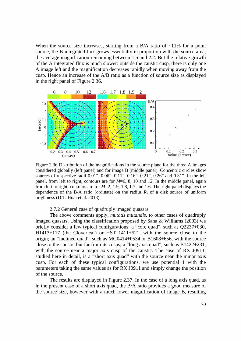
70

When the source size increases, starting from a B/A ratio of ~11% for a point source, the B integrated flux grows essentially in proportion with the source area, the average magnification remaining between 1.5 and 2.2. But the relative growth of the A integrated flux is much slower: outside the caustic cusp, there is only one A image left and the magnification decreases rapidly when moving away from the cusp. Hence an increase of the A/B ratio as a function of source size as displayed in the right panel of Figure 2.36.

Figure 2.36 Distribution of the magnifications in the source plane for the three A images considered globally (left panel) and for image B (middle panel). Concentric circles show sources of respective radii 0.01”, 0.06”, 0.11”, 0.16”, 0.21”, 0.26” and 0.31”. In the left panel, from left to right, contours are for M=6, 8, 10 and 12. In the middle panel, again from left to right, contours are for M=2, 1.9, 1.8, 1.7 and 1.6. The right panel displays the dependence of the B/A ratio (ordinate) on the radius Rs of a disk source of uniform brightness (D.T. Hoai et al. 2013).

2.7.2 General case of quadruply imaged quasars The above comments apply, mutatis mutandis, to other cases of quadruply

imaged quasars. Using the classification proposed by Saha & Williams (2003) we briefly consider a few typical configurations: a “core quad”, such as Q2237+030, H1413+117 (the Cloverleaf) or HST 1411+521, with the source close to the origin; an “inclined quad”, such as MG0414+0534 or B1608+656, with the source close to the caustic but far from its cusps; a “long axis quad”, such as B1422+231, with the source near a major axis cusp of the caustic. The case of RX J0911, studied here in detail, is a “short axis quad” with the source near the minor axis cusp. For each of these typical configurations, we use potential 1 with the parameters taking the same values as for RX J0911 and simply change the position of the source.

The results are displayed in Figure 2.37. In the case of a long axis quad, as in the present case of a short axis quad, the B/A ratio provides a good measure of the source size, however with a much lower magnification of image B, resulting

0.3

0.2

0.1

0

−0.1

−0.2

0.2 0.3 0.4 0.5 0.6 0.7 (arcsec) Radius (arcsec)

0 0.1 0.2 0.3

0.4

0.3

0.2

0.1

B/A

(ar

csec

)

6 8 10 12 1.6 1.7 1.8 1.9 2

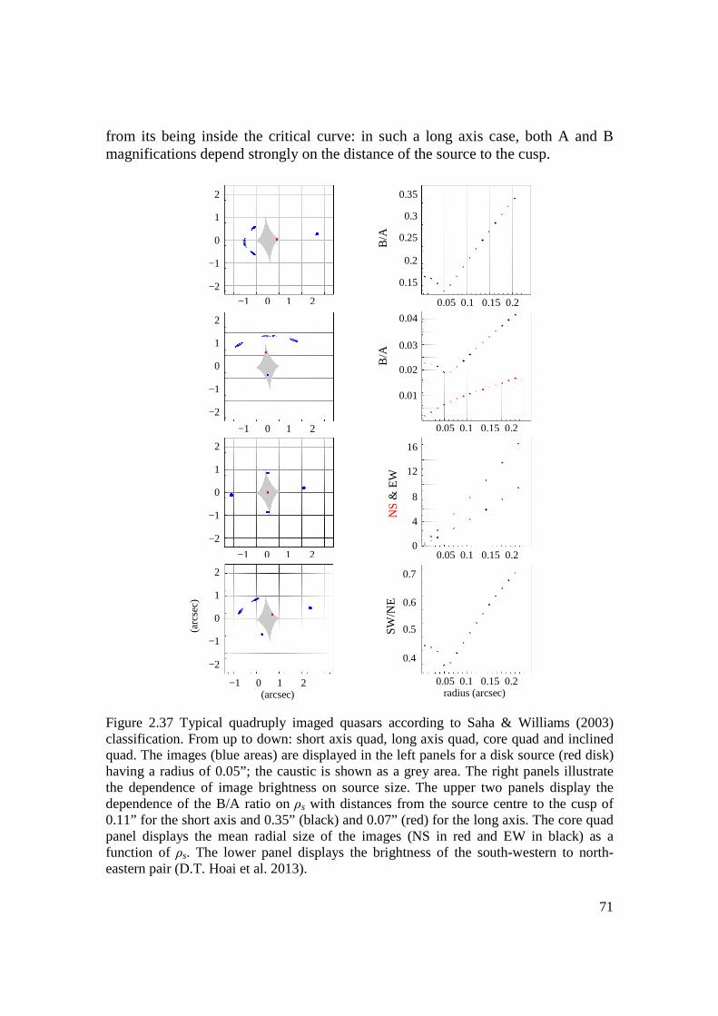
71

from its being inside the critical curve: in such a long axis case, both A and B magnifications depend strongly on the distance of the source to the cusp.

Figure 2.37 Typical quadruply imaged quasars according to Saha & Williams (2003) classification. From up to down: short axis quad, long axis quad, core quad and inclined quad. The images (blue areas) are displayed in the left panels for a disk source (red disk) having a radius of 0.05”; the caustic is shown as a grey area. The right panels illustrate the dependence of image brightness on source size. The upper two panels display the dependence of the B/A ratio on ρs with distances from the source centre to the cusp of 0.11” for the short axis and 0.35” (black) and 0.07” (red) for the long axis. The core quad panel displays the mean radial size of the images (NS in red and EW in black) as a function of ρs. The lower panel displays the brightness of the south-western to north-eastern pair (D.T. Hoai et al. 2013).

(arcsec)

(arc

sec)

radius (arcsec)

B/A

B

/A

NS

& E

W

SW

/NE

0.35

0.3

0.25

0.2

0.15

0.04

0.03

0.02

0.01

16

12

8

4

0

0.7

0.6

0.5

0.4

0.05 0.1 0.15 0.2

0.05 0.1 0.15 0.2

0.05 0.1 0.15 0.2

0.05 0.1 0.15 0.2

2

1

0

−1

−2

2

1

0

−1

−2

2

1

0

−1

−2

2

1

0

−1

−2

−1 0 1 2

−1 0 1 2

−1 0 1 2

−1 0 1 2

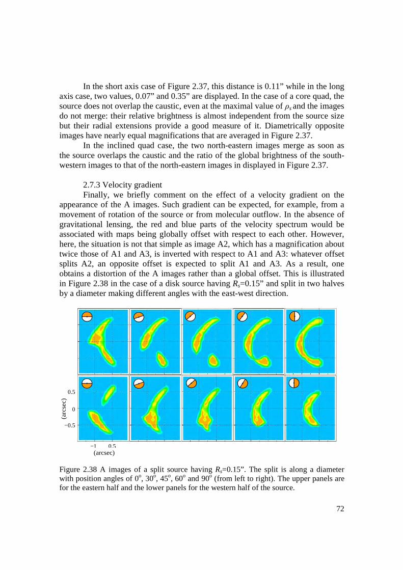
72

In the short axis case of Figure 2.37, this distance is 0.11” while in the long

axis case, two values, 0.07” and 0.35” are displayed. In the case of a core quad, the source does not overlap the caustic, even at the maximal value of ρs and the images do not merge: their relative brightness is almost independent from the source size but their radial extensions provide a good measure of it. Diametrically opposite images have nearly equal magnifications that are averaged in Figure 2.37.

In the inclined quad case, the two north-eastern images merge as soon as the source overlaps the caustic and the ratio of the global brightness of the south-western images to that of the north-eastern images in displayed in Figure 2.37.

2.7.3 Velocity gradient Finally, we briefly comment on the effect of a velocity gradient on the

appearance of the A images. Such gradient can be expected, for example, from a movement of rotation of the source or from molecular outflow. In the absence of gravitational lensing, the red and blue parts of the velocity spectrum would be associated with maps being globally offset with respect to each other. However, here, the situation is not that simple as image A2, which has a magnification about twice those of A1 and A3, is inverted with respect to A1 and A3: whatever offset splits A2, an opposite offset is expected to split A1 and A3. As a result, one obtains a distortion of the A images rather than a global offset. This is illustrated in Figure 2.38 in the case of a disk source having Rs=0.15” and split in two halves by a diameter making different angles with the east-west direction.

Figure 2.38 A images of a split source having Rs=0.15”. The split is along a diameter with position angles of 0o, 30o, 45o, 60o and 90o (from left to right). The upper panels are for the eastern half and the lower panels for the western half of the source.

0.5

0

−0.5

−1 0.5 (arcsec)

(arc

sec)

73

However, the use of simple effective gravity potentials to describe lensing is an approximation to a more complex reality and the predictions illustrated here are merely a guide for the analysis of future observations. Precise and conclusive results can only be obtained following a careful “dissection” of the “anatomy” of the source and lens configurations, in the wake of similar analyses made by Suyu & al. in the case of B1608+656 (Suyu & Blandford 2005, Suyu & al. 2009). As convolution with the interferometer beam smears the images, making their interpretation more difficult than suggested here, the present work can help with the evaluation of the related requirements in terms of beam and of observation time.

2.8 Summary and conclusion

The mapping of an extended source onto its gravitationally lensed images has been studied with the aim of guiding the analysis of high resolution observations of the host galaxy of QSO RX J0911 and of similar high redshift quasars: the results are general enough to be of interest to the study of other multiply imaged galaxies. Using simple effective potentials, the general features of the lensing mechanism have been recalled and explicit analytic relations have been given that are of help in understanding the main features. Particular attention has been paid to the behaviour of the lens equation when the source approaches the caustic and a simple potential has been used to illustrate the main features. The study of the particular case of QSO RX J0911 has been made using two different potentials: potential 1 describes the lensing effect of the galaxy cluster using an external shear and the lens equation was solved in a straightforward and transparent manner; potential 2 describes the lensing effect of the galaxy cluster and of the satellite galaxy G’ using separate explicit potentials and the lens equation was solved using the publicly available LENSTOOL package. In both cases the vicinity of the caustic was explored with great care. A detailed comparison of the images produced by each of these potentials has shown small but significant differences resulting from the closer proximity of the source from the caustic in the case of potential 2. It has been commented that we are unable to tell which of potentials 1 and 2 is better adapted to the task of evaluating the size and properties of the host galaxy of RX J0911 and that both will be used on an equal footing, hoping that the differences between their predictions will give a reasonable estimate of the systematic uncertainties attached to the imperfection of the lens model.

The use of variables sensitive to the source size has been suggested, including the dependence of the relative B/A image brightness. Typical quadruply imaged quasar configurations have been used as illustrations. The effect of strong lensing on a velocity gradient has been briefly considered.

74

3. Modelling the host galaxy of QSO RX J0911

3.1 Introduction Having now control over the gravitational lensing mechanism, we are in a

position to compare the RX J0911 data collected using the PdBI with the predictions of any model of the source. In practice, we shall proceed as follows:

− In a first step we model the source by creating a source map: to each node (i,j) of the source grid, having coordinates (xsi, ysj), we associate a brightness Bij.

− In a second step, we calculate the images predicted by the model by lensing the source: to each node (i,j) of the source grid we associate Nij images having positions in the image plane xijk, yijk and magnification Mijk, with k running from 1 to Nij. The values of xijk, yijk, and Mijk have been calculated once for all. We build an image map of 6”×6” made of 512×512 pixels, namely with a pixel size of ~11.7×11.7 mas2. Each pixel is given a brightness that is the product by the primary beam of the sum of BijMijk where the sum extents over all values of (i,j,k) such that the kth image of the source has its coordinates within that pixel.

− In a third step, we Fourier transform the image map to the u-v plane. This is done using the GILDAS package, the result being given as two visibility lists in the u-v plane, one of their real parts, the other of their imaginary parts, making its comparison with data easy. For each interval of time during which the PdBi collects data, namely 45 s, each baseline produces two measurements, an amplitude and a phase, that are equivalently expressed as a complex visibility. The data are therefore available, for each frequency bin, as a list of visibilities with associated values of u and v. The Fourier transform of the images produced by the model is of course frequency independent but is given by GILDAS as a similar list of visibilities associated with the same u and v values as for the data.

− In a fourth step, we calculate the value of χ2 describing the match between the observed and modelled u-v lists of visibilities and iterate the procedure by adjusting the model parameters to obtain the best possible fit, namely the smallest possible value of χ2. The total computer time necessary to calculate the χ2 associated with a given source position is ~3 s for a typical source size.

The present chapter addresses each of these steps in turn. 3.2 Astrometry A preliminary requirement is to position the model parameters, including

the source position, in the same frame of coordinates in which the PdBI data are referred. A first approximation is simply to locate the lens G at its position given by the HST (Kneib et al., 2000), namely RAHST=09:11:27.55900 and DecHST=05:50.54.200. However, we may expect some differences, at the scale of 100 mas or so, between the HST and PdBI reference frames. What we need are the coordinates of G in the PdBI frame of reference. To obtain these, we use the

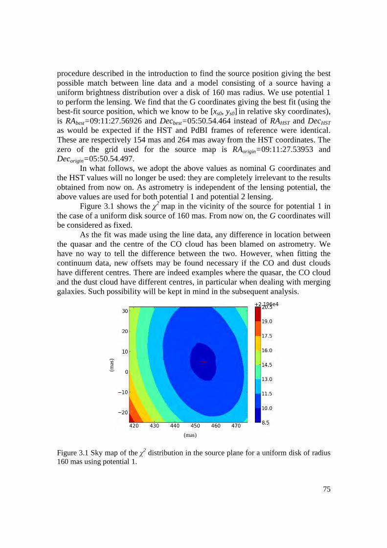
75

procedure described in the introduction to find the source position giving the best possible match between line data and a model consisting of a source having a uniform brightness distribution over a disk of 160 mas radius. We use potential 1 to perform the lensing. We find that the G coordinates giving the best fit (using the best-fit source position, which we know to be [xs0, ys0] in relative sky coordinates), is RAbest=09:11:27.56926 and Decbest=05:50.54.464 instead of RAHST and DecHST as would be expected if the HST and PdBI frames of reference were identical. These are respectively 154 mas and 264 mas away from the HST coordinates. The zero of the grid used for the source map is RAorigin=09:11:27.53953 and Decorigin=05:50.54.497.

In what follows, we adopt the above values as nominal G coordinates and the HST values will no longer be used: they are completely irrelevant to the results obtained from now on. As astrometry is independent of the lensing potential, the above values are used for both potential 1 and potential 2 lensing.

Figure 3.1 shows the χ2 map in the vicinity of the source for potential 1 in the case of a uniform disk source of 160 mas. From now on, the G coordinates will be considered as fixed.

As the fit was made using the line data, any difference in location between the quasar and the centre of the CO cloud has been blamed on astrometry. We have no way to tell the difference between the two. However, when fitting the continuum data, new offsets may be found necessary if the CO and dust clouds have different centres. There are indeed examples where the quasar, the CO cloud and the dust cloud have different centres, in particular when dealing with merging galaxies. Such possibility will be kept in mind in the subsequent analysis.

Figure 3.1 Sky map of the χ2 distribution in the source plane for a uniform disk of radius 160 mas using potential 1.

(mas

)

(mas)

76

In order to get an idea of the robustness of this result, we compare it with that obtained using a Gaussian brightness distribution having the same <r 2>½ and we repeat the exercise using the continuum data rather than the line data, the size of the disk being now 60 mas instead of 160 mas. The results are summarized in Table 3.1. For comparison, we also list in the table and show in the figure the result of the fit of the HST quasar images (of course, not in the u-v plane!)

Table 3.1 Astrometry results obtained on the line and continuum using potential 1 for

uniform and Gaussian brightness distributions of the source.

Brightness distribution

Velocity range

Best-fit xs Best-fit ys Best-fit χ2/dof

HST point images

IR 446 (8) 33 (4) −

Uniform ρ=113 mas

Line 454 (15) 5 (21) 0.80123

Gaussian ρ=148 mas

Line 460 (15) 23 (19) 0.80116

Uniform ρ=39 mas

Continuum 474 (16) 21 (18) 0.80954

Gaussian ρ=52 mas

Continuum 474 (16) 27 (18) 0.80955

The results call for a number of comments. − The error bars are of the order of 16 mas in right ascension and 20 mas in

declination; the systematic differences between a uniform and Gaussian brightness distributions are smaller than that, giving confidence in the robustness of the result.

− The differences between HST, CO(7-6) line and continuum are not very significant and do not give any evidence for different source positions in the three cases.

− Note that uncertainties in y are larger than in x for the radio interferometer data because of the beam shape while the opposite is true in the infrared data.

3.3 Effects contributing to χ2 There are 27420 degrees of freedom (914 measurements of two numbers

each for 15 baselines) and the χ2 values are nearly 20% lower. Before proceeding further, we discuss the effects that contribute to χ2. We

may expect contributions from the inadequacy of the model (either the model of the source or the model of the lens or both) and contributions from noise, including several possible components.

It is easy to see that the contribution of the model is negligible. Concerning the model of the lens, we choose four source positions that are separated from that

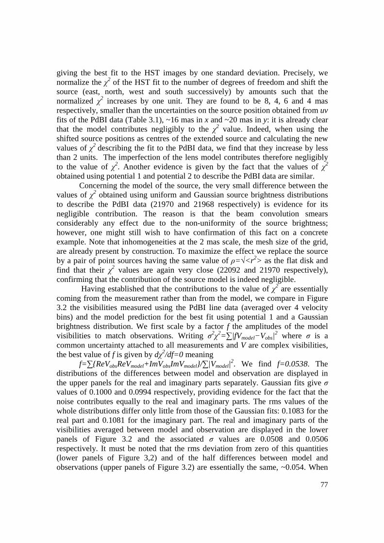
77

giving the best fit to the HST images by one standard deviation. Precisely, we normalize the χ2 of the HST fit to the number of degrees of freedom and shift the source (east, north, west and south successively) by amounts such that the normalized χ2 increases by one unit. They are found to be 8, 4, 6 and 4 mas respectively, smaller than the uncertainties on the source position obtained from uv fits of the PdBI data (Table 3.1), ~16 mas in x and ~20 mas in y: it is already clear that the model contributes negligibly to the χ2 value. Indeed, when using the shifted source positions as centres of the extended source and calculating the new values of χ2 describing the fit to the PdBI data, we find that they increase by less than 2 units. The imperfection of the lens model contributes therefore negligibly to the value of χ2. Another evidence is given by the fact that the values of χ2 obtained using potential 1 and potential 2 to describe the PdBI data are similar.

Concerning the model of the source, the very small difference between the values of χ2 obtained using uniform and Gaussian source brightness distributions to describe the PdBI data (21970 and 21968 respectively) is evidence for its negligible contribution. The reason is that the beam convolution smears considerably any effect due to the non-uniformity of the source brightness; however, one might still wish to have confirmation of this fact on a concrete example. Note that inhomogeneities at the 2 mas scale, the mesh size of the grid, are already present by construction. To maximize the effect we replace the source by a pair of point sources having the same value of ρ=√<r 2> as the flat disk and find that their χ2 values are again very close (22092 and 21970 respectively), confirming that the contribution of the source model is indeed negligible.

Having established that the contributions to the value of χ2 are essentially coming from the measurement rather than from the model, we compare in Figure 3.2 the visibilities measured using the PdBI line data (averaged over 4 velocity bins) and the model prediction for the best fit using potential 1 and a Gaussian brightness distribution. We first scale by a factor f the amplitudes of the model visibilities to match observations. Writing σ2χ2=∑|fVmodel−Vobs|

2 where σ is a common uncertainty attached to all measurements and V are complex visibilities, the best value of f is given by dχ2/df=0 meaning

f=∑ReVobsReVmodel+ImVobsImVmodel/∑|Vmodel|2. We find f=0.0538. The

distributions of the differences between model and observation are displayed in the upper panels for the real and imaginary parts separately. Gaussian fits give σ values of 0.1000 and 0.0994 respectively, providing evidence for the fact that the noise contributes equally to the real and imaginary parts. The rms values of the whole distributions differ only little from those of the Gaussian fits: 0.1083 for the real part and 0.1081 for the imaginary part. The real and imaginary parts of the visibilities averaged between model and observation are displayed in the lower panels of Figure 3.2 and the associated σ values are 0.0508 and 0.0506 respectively. It must be noted that the rms deviation from zero of this quantities (lower panels of Figure 3,2) and of the half differences between model and observations (upper panels of Figure 3.2) are essentially the same, ~0.054. When

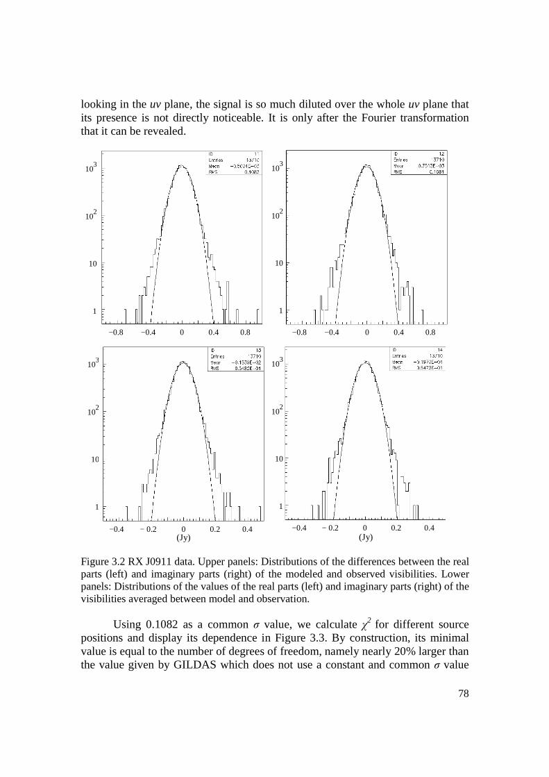
78

looking in the uv plane, the signal is so much diluted over the whole uv plane that its presence is not directly noticeable. It is only after the Fourier transformation that it can be revealed.

Figure 3.2 RX J0911 data. Upper panels: Distributions of the differences between the real parts (left) and imaginary parts (right) of the modeled and observed visibilities. Lower panels: Distributions of the values of the real parts (left) and imaginary parts (right) of the visibilities averaged between model and observation.

Using 0.1082 as a common σ value, we calculate χ2 for different source

positions and display its dependence in Figure 3.3. By construction, its minimal value is equal to the number of degrees of freedom, namely nearly 20% larger than the value given by GILDAS which does not use a constant and common σ value

−0.8 −0.4 0 0.4 0.8

103

102

10

1

−0.4 − 0.2 0 0.2 0.4 −0.4 − 0.2 0 0.2 0.4 (Jy) (Jy)

103

102

10

1

103

102

10

1

103

102

10

1

−0.8 −0.4 0 0.4 0.8

79

but accounts for its dependence on time and baseline. It is however remarkable that the minima of the GILDAS χ2 and of that obtained using a common and constant value of σ are less than 30 mas away from each other, providing evidence for the robustness of the results with respect to the weights used in the definition of χ2. It is important to remark that the GILDAS χ2 uses a normalization factor f

Figure 3.3 Source map (scale is mas) of χ2 using a common and constant weight (σ =0.1082). The GILDAS χ2 is minimal at the origin of coordinates (red cross). calculated for variable σ values and therefore different from that calculated above using a common and constant σ (0.0615 instead of 0.0538). Indeed, the weights used by GILDAS are far from being common to all baselines and constant with time. Figure 3.4 shows their dependence on measurement number for each of the 15 baselines separately. Figure 3.5 (left) zooms on details of the weight distribution showing the effect of stops occurring after~25 min of measurement for quasar calibration. Figure 3.6 shows the distribution of the GILDAS weights and compares them with 10−6/(0.1082)2, the value corresponding to a common and constant σ.

We see from Figure 3.6 that the GILDAS weights vary from ~10−5 to ~2.5 10−4 meaning noise values from ~60 to ~310. This is a large span. In this context, we note that the cosmic microwave background is a constant and antenna independent contribution; electronics noise is nearly constant with time but baseline dependent; atmospheric noise is nearly baseline independent but depends on time (weather conditions and elevation, meaning thickness of atmosphere traversed).

80

Figure 3.4 Dependence on measurement number (from the last to the first) of the weights used by GILDAS for each of the 15 baselines. Note that 13710 visibilities divided by 15 baselines means 914 measurements of 45 s each. There are two measurements per bin, meaning that the weights should be divided by 2.

Figure 3.5 Left: zoom on the dependence of the GILDAS weight on measurement number for baseline 1 showing regular jumps. Right: distribution of the difference between the GILDAS weights of two successive measurements as a function of measurement numbers. The stops associated with the jumps visible in the left panel appear now as regular spikes.

Jumps x10

−2

0.14

0.1

0.06

0.02

0 40 80 120 160 0 200 400 600 800

10−4

10−5

10−6

10−7

0 200 400 600 800 1000

−104

81

Figure 3.6 Distribution of the GILDAS weights. The red arrow corresponds to a constant common weight.

3.4 Source size In the present section, we model the source with a circular symmetric

brightness distribution, using a single parameter ρ=<√ r2> to define its size. Note that for a uniform distribution of radius R, ρ=R/√2 and for a Gaussian, ρ=σ√2=FWHM/1.662. The data are averaged over four central velocity bins on the line and 35 velocity bins in the continuum, on either sides of the line (18 at higher velocities and 17 at lower velocities with a 3-bin no man’s land on each side of the line). Moreover, the continuum contribution, evaluated from 35 velocity bins bracketing the line (17 below and 18 above), is subtracted. The astrometry is fixed at the values listed in Table 3.1. The number of degrees of freedom is 13710(−1), the averaging being done in GILDAS with the noise divided by √4 and √35 for the line and continuum respectively.

The results are listed in Table 3.2 and illustrated in Figure 3.7. The results obtained using potential 2 differ by less than a standard deviation from those of Anh et al. (2013); precisely by 14 mas on the line and 7 mas in the continuum, with respective uncertainties of 17 and 11 mas. A difference between these is the fact that the LENSTOOL facility of dealing with extended sources was used in Anh et al. (2013) while it no longer is here. Another difference, in the line case, is that we are only averaging four velocity bins while six were averaged in Anh et al. (2013), in which case the noise was smaller by a factor √(6/4)=1.22, which explains the larger value of χ2.

82

However, the difference between potential 1 and potential 2 is significant. In the case of a Gaussian brightness distribution, they predict respectively 148±20 mas and 105±16 mas on the line and 55±21 mas and 17±10 mas in the continuum, meaning differences of 43±26 mas and 38±23 mas. The weighted averages of the potentials 1 and 2 predictions are 122±12 mas and 24±9 mas compared with 91±12 mas and 24±5 mas quoted in Anh et al. (2013). However, this does not include the systematic uncertainty associated with the imperfection of the lens and source models.

Another comment concerns the values of the uncertainties obtained using potentials 1 and 2: the former are larger than the latter in absolute value but smaller in relative value.

Table 3.2 Best fit results on the source size

Velocity range Brightness distribution

Potential 1 Potential 2

ρ (mas) χ2 ρ (mas) χ2

Line Uniform 115(13) 21969 78(10) 21974 Gaussian 148(20) 21969 105(16) 21971 Anh et al 91(12) 24768

Continuum Uniform 37(14) 22200 14(5) 22198 Gaussian 55(21) 22201 17(10) 22198 Anh et al 24(5) 22190

Figure 3.7 χ2 distributions for the line (left panel) and the continuum (middle panel) using potentials 1 (blue) and 2 (red) as a function of the source size ρ (mas). The full line is for a uniform brightness distribution, the dashed line for a Gaussian and the dash-dotted line for the mixed profile displayed in the right panel (central disk with Gaussian edges).

In order to estimate the effect of an imperfect astrometry, we repeat the fits

with the coordinate system of the model shifted by one standard deviation in both

DISK R=ρ√2 GAUSSIAN σ=R/2.355 ρ =<r2>½

R=1.168 ρ

R/2 σ

100

80

60

40

20

0

30

25

20

15

10

5

+2.219e4

0 40 80 120 ρ (mas) ρ (mas)

0 50 100 150 200

+2.196e3

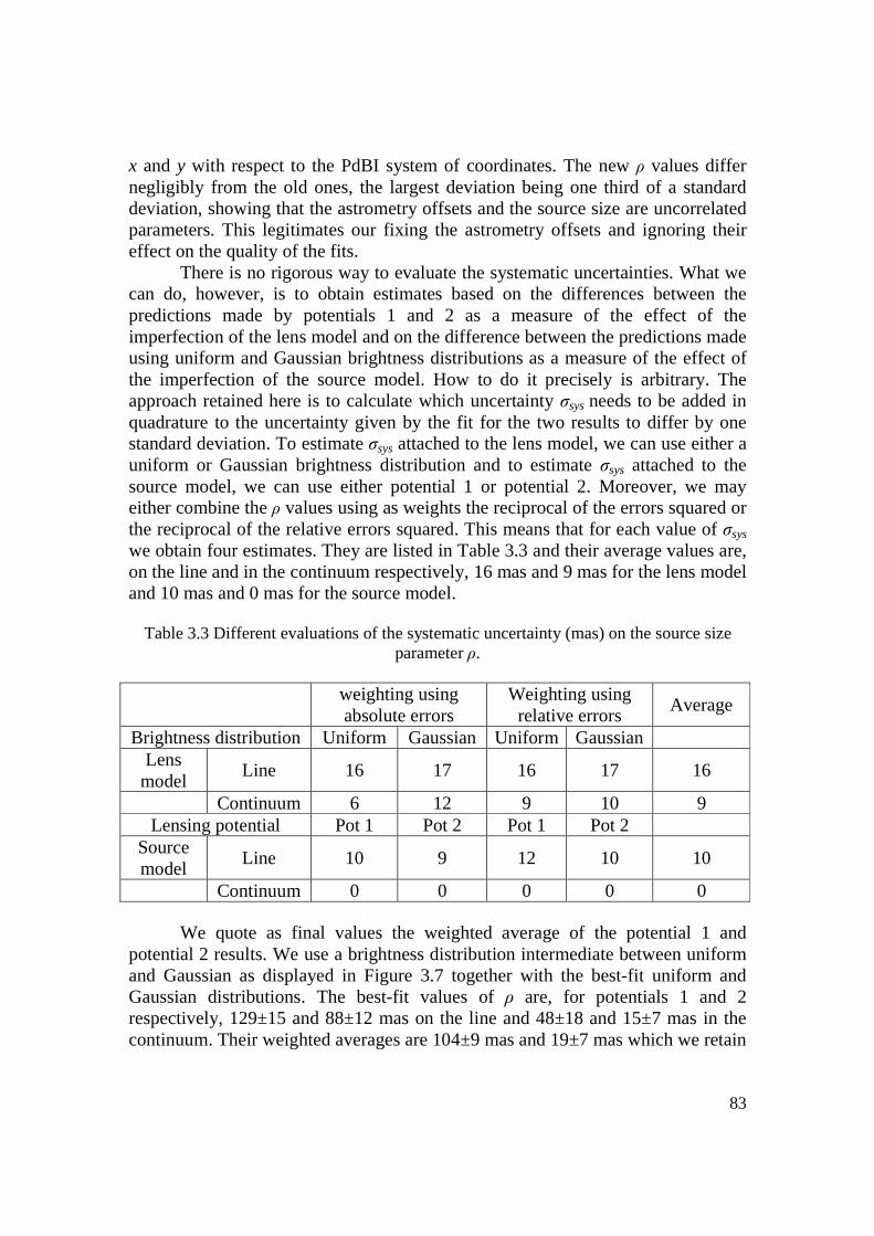
83

x and y with respect to the PdBI system of coordinates. The new ρ values differ negligibly from the old ones, the largest deviation being one third of a standard deviation, showing that the astrometry offsets and the source size are uncorrelated parameters. This legitimates our fixing the astrometry offsets and ignoring their effect on the quality of the fits.

There is no rigorous way to evaluate the systematic uncertainties. What we can do, however, is to obtain estimates based on the differences between the predictions made by potentials 1 and 2 as a measure of the effect of the imperfection of the lens model and on the difference between the predictions made using uniform and Gaussian brightness distributions as a measure of the effect of the imperfection of the source model. How to do it precisely is arbitrary. The approach retained here is to calculate which uncertainty σsys needs to be added in quadrature to the uncertainty given by the fit for the two results to differ by one standard deviation. To estimate σsys attached to the lens model, we can use either a uniform or Gaussian brightness distribution and to estimate σsys attached to the source model, we can use either potential 1 or potential 2. Moreover, we may either combine the ρ values using as weights the reciprocal of the errors squared or the reciprocal of the relative errors squared. This means that for each value of σsys we obtain four estimates. They are listed in Table 3.3 and their average values are, on the line and in the continuum respectively, 16 mas and 9 mas for the lens model and 10 mas and 0 mas for the source model.

Table 3.3 Different evaluations of the systematic uncertainty (mas) on the source size

parameter ρ.

weighting using absolute errors

Weighting using relative errors

Average

Brightness distribution Uniform Gaussian Uniform Gaussian Lens model

Line 16 17 16 17 16

Continuum 6 12 9 10 9 Lensing potential Pot 1 Pot 2 Pot 1 Pot 2

Source model

Line 10 9 12 10 10

Continuum 0 0 0 0 0

We quote as final values the weighted average of the potential 1 and potential 2 results. We use a brightness distribution intermediate between uniform and Gaussian as displayed in Figure 3.7 together with the best-fit uniform and Gaussian distributions. The best-fit values of ρ are, for potentials 1 and 2 respectively, 129±15 and 88±12 mas on the line and 48±18 and 15±7 mas in the continuum. Their weighted averages are 104±9 mas and 19±7 mas which we retain

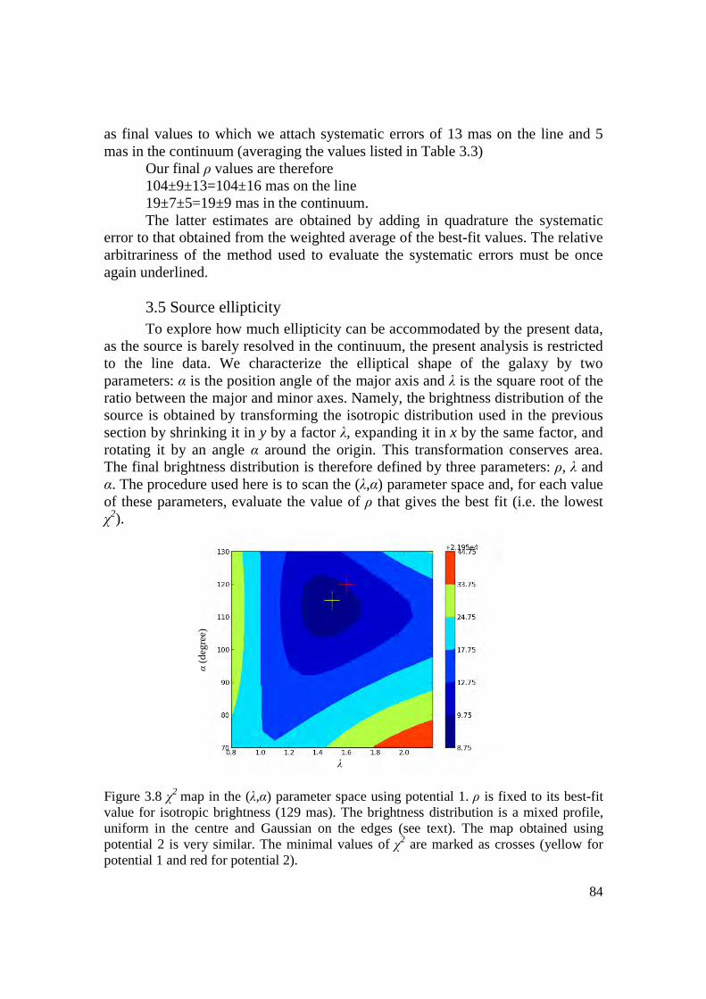
84

as final values to which we attach systematic errors of 13 mas on the line and 5 mas in the continuum (averaging the values listed in Table 3.3) Our final ρ values are therefore 104±9±13=104±16 mas on the line 19±7±5=19±9 mas in the continuum. The latter estimates are obtained by adding in quadrature the systematic error to that obtained from the weighted average of the best-fit values. The relative arbitrariness of the method used to evaluate the systematic errors must be once again underlined.

3.5 Source ellipticity To explore how much ellipticity can be accommodated by the present data, as the source is barely resolved in the continuum, the present analysis is restricted to the line data. We characterize the elliptical shape of the galaxy by two parameters: α is the position angle of the major axis and λ is the square root of the ratio between the major and minor axes. Namely, the brightness distribution of the source is obtained by transforming the isotropic distribution used in the previous section by shrinking it in y by a factor λ, expanding it in x by the same factor, and rotating it by an angle α around the origin. This transformation conserves area. The final brightness distribution is therefore defined by three parameters: ρ, λ and α. The procedure used here is to scan the (λ,α) parameter space and, for each value of these parameters, evaluate the value of ρ that gives the best fit (i.e. the lowest χ2).

Figure 3.8 χ2 map in the (λ,α) parameter space using potential 1. ρ is fixed to its best-fit value for isotropic brightness (129 mas). The brightness distribution is a mixed profile, uniform in the centre and Gaussian on the edges (see text). The map obtained using potential 2 is very similar. The minimal values of χ2 are marked as crosses (yellow for potential 1 and red for potential 2).

λ

α (d

egre

e)

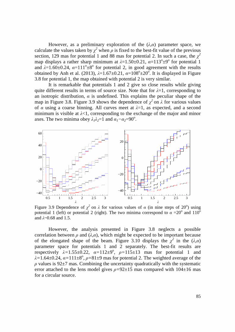
85

However, as a preliminary exploration of the (λ,α) parameter space, we calculate the values taken by χ2 when ρ is fixed to the best-fit value of the previous section, 129 mas for potential 1 and 88 mas for potential 2. In such a case, the χ2

map displays a rather sharp minimum at λ=1.50±0.21, α=113o±9o for potential 1 and λ=1.60±0.24, α=111o±8o for potential 2, in good agreement with the results obtained by Anh et al. (2013), λ=1.67±0.21, α=108o±20o. It is displayed in Figure 3.8 for potential 1, the map obtained with potential 2 is very similar.

It is remarkable that potentials 1 and 2 give so close results while giving quite different results in terms of source size. Note that for λ=1, corresponding to an isotropic distribution, α is undefined. This explains the peculiar shape of the map in Figure 3.8. Figure 3.9 shows the dependence of χ2 on λ for various values of α using a coarse binning. All curves meet at λ=1, as expected, and a second minimum is visible at λ<1, corresponding to the exchange of the major and minor axes. The two minima obey λ1λ2=1 and α1−α2=90o.

Figure 3.9 Dependence of χ2 on λ for various values of α (in nine steps of 20o) using potential 1 (left) or potential 2 (right). The two minima correspond to α =20o and 110o and λ~0.68 and 1.5.

However, the analysis presented in Figure 3.8 neglects a possible

correlation between ρ and (λ,α), which might be expected to be important because of the elongated shape of the beam. Figure 3.10 displays the χ2 in the (λ,α) parameter space for potentials 1 and 2 separately. The best-fit results are respectively λ=1.55±0.22, α=112±9o, ρ=115±13 mas for potential 1 and λ=1.64±0.24, α=111±8o, ρ=81±9 mas for potential 2. The weighted average of the ρ values is 92±7 mas. Combining the uncertainty quadratically with the systematic error attached to the lens model gives ρ=92±15 mas compared with 104±16 mas for a circular source.

0.5 1 1.5 2 2.5 3

20

0

−20

−40

0.5 1 1.5 2 2.5 3

60

40

20

0

−20

−40

λ λ

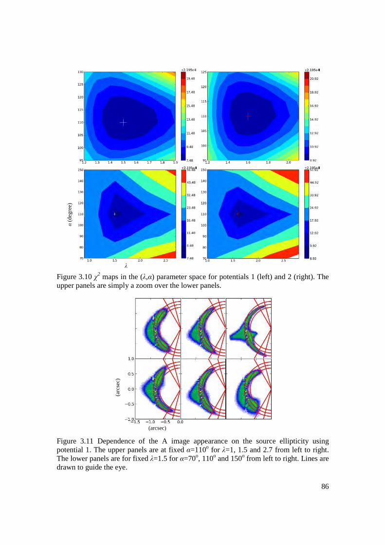
86

Figure 3.10 χ2 maps in the (λ,α) parameter space for potentials 1 (left) and 2 (right). The upper panels are simply a zoom over the lower panels.

Figure 3.11 Dependence of the A image appearance on the source ellipticity using potential 1. The upper panels are at fixed α=110o for λ=1, 1.5 and 2.7 from left to right. The lower panels are for fixed λ=1.5 for α=70o, 110o and 150o from left to right. Lines are drawn to guide the eye.

(arcsec)

(arc

sec)

α (d

eg

ree)

λ

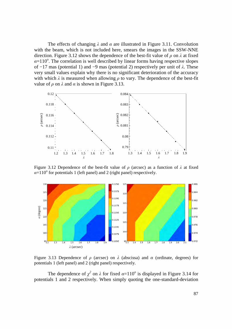
87

The effects of changing λ and α are illustrated in Figure 3.11. Convolution with the beam, which is not included here, smears the images in the SSW-NNE direction. Figure 3.12 shows the dependence of the best-fit value of ρ on λ at fixed α=110o. The correlation is well described by linear forms having respective slopes of −17 mas (potential 1) and −9 mas (potential 2) respectively per unit of λ. These very small values explain why there is no significant deterioration of the accuracy with which λ is measured when allowing ρ to vary. The dependence of the best-fit value of ρ on λ and α is shown in Figure 3.13.

Figure 3.12 Dependence of the best-fit value of ρ (arcsec) as a function of λ at fixed α=110o for potentials 1 (left panel) and 2 (right panel) respectively.

Figure 3.13 Dependence of ρ (arcsec) on λ (abscissa) and α (ordinate, degrees) for potentials 1 (left panel) and 2 (right panel) respectively.

The dependence of χ2 on λ for fixed α=110o is displayed in Figure 3.14 for

potentials 1 and 2 respectively. When simply quoting the one-standard-deviation

λ (arcsec)

α (d

egre

e)

0.12

0.118

0.116

0.114

0.112

0.11

0.084

0.083

0.082

0.081

0.08

0.79

1.2 1.3 1.4 1.5 1.6 1.7 1.8 λ

1.3 1.4 1.5 1.6 1.7 1.8 1.9 λ

ρ (a

rcse

c)

ρ (a

rcse

c)

88

error, it would seem that the circular source hypothesis is only barely rejected to less than 3 standard deviations: for potential 1 1.55±0.22 means 2.5 standard deviations and for potential 2 λ=1.64±0.24 means 2.7 standard deviations. However, because of the asymmetric dependence of χ2 on λ, the circular source hypothesis is in fact rejected to better than 3 standard deviations. Quoting 3-standard deviation uncertainties, defined as producing an increase of χ2 by 9 units, we obtain λ=1.52+1.08−0.48 for potential 1 and 1.63+1.03−0.55 for potential 2.

Figure 3.14 Dependence of χ2 on λ for fixed α=110o and for potentials 1 (left panel) and 2 (right panel) respectively. Horizontal lines show the 2 and 3 standard deviation values (respectively 4 and 9 units above minimum).

Figure 3.15 Maps of the best-fit sources for potential 1 (left panel) and 2 (right panel) respectively. Both sources are centred at zero and the coordinates are measured in arcseconds.

21968

21966

21964

21962

21960

21958

1 1.2 1.4 1.6 1.8 2 2.2 2.4 2.6 1 1.2 1.4 1.6 1.8 2 2.2 2.4 2.6 2.8 λ

89

The remarkable similarity between the two results suggests that the systematic uncertainty associated with imperfections of the lens model can safely be neglected. Keeping as one-standard deviation uncertainties those obtained by dividing by 3 those quoted above and averaging the potential 1 and 2 results gives λ=1.60+0.35−0.18 and α=111o±9o, 3.3 standard deviations away from a circular source hypothesis. This estimate neglects systematic uncertainties attached to the imperfection of the source model. However, it is reasonable to think that having allowed for the source to be elliptic should take care of most of these.

Figure 3.15 displays the best-fit source brightness in the source plane for potentials 1 and 2 separately.

3.6 B/A brightness ratio As was remarked in the Section 2.7.1, the B/A brightness ratio depends on

the source size and can in principle be used to evaluate it. For this evaluation, we use the clean map of the flux measured on the

CO(7-6) line, including the four central velocity bins. As the spectral flux density of each pixel is given in Jy/beam, the total flux (in Jy) in a given area that covers N pixels, is F=S0/B0 ∑i fi where fi is the flux density per beam in pixel i, S0 is the area of one pixel (0.0064 arcsec2) and B0 is the area of the beam, 2πσ1σ2 where σ1

and σ2 are the sigmas of the Gaussians describing the synthesized beam along its major and minor axes respectively, namely 1.133 a1a2 with a1 and a2 being the corresponding FWHMs. Here, a1=0.72 and a2=0.27 arcsec namely S0/B0=0.0064/0.220=0.0291.

Figure 3.16 Dependence of the B/A ratio on ρ (mas) for an elliptical source having λ and α fixed at their best-fit values and a mixed uniform/Gaussian brightness distribution. The prediction obtained using potential 1 is shown in blue, that using potential 2, in red. The measured B/A values are shown as bands ±1 standard deviation wide, dark blue for Weiss et al. (2012) and cyan for the present work. The best-fit value of ρ obtained here, 92±15 mas, is shown as a vertical green band.

ρ (mas)

B/A

90

The noise per beam and frequency channel is 1.74 mJy, namely 1.74/√4=0.87 mJy/beam (or 1.74/√6=0.71 mJy/beam). For N pixels, this number must be multiplied by √(NS0/B0) to obtain the uncertainty ∆Fline=0.1484√N mJy (or 0.1211√N mJy ).

The result is 26.0±2.1 mJy for the A images (12×24 pixels) and 2.9±1.2 mJy for B, after subtraction of the contribution of the continuum. Hence, B/A=11.2±4.7%. This result is 2 standard deviations smaller than the result obtained by Weiss et al. (2012), 21±1 %, with a better resolution.

Figure 3.16 compares these results with the predictions of the model using the mixed disk+Gaussian brightness distribution for the source with λ and α fixed at their best-fit values. Our previous best estimate of ρ, 92±15 mas, corresponds to B/A=0.150±0.025 when averaging over potentials 1 and 2. Conversely, B/A=0.20±0.01, weighted average of our and Weiss et al. (2012) measurements, means ρ values of the order of 120±15 mas. Combining all results together gives ρ=106±15 mas and B/A=0.19±0.01.

3.7 Velocity gradient Evidence for the presence of a velocity gradient was presented in Anh et al.

(2013) by comparing the clean map A images associated with the red and blue halves of the CO line respectively. Here, we extend this study to the uv plane. We use the best-fit model of the source and lens separately its eastern and western halves from which we build two image maps, which we Fourier transform to the uv plane using GILDAS. We obtain this way two lists of complex visibilities, one for the eastern half, the other for the western half, which we call V–

i and V+i.

Similarly, we average the data over two intervals of four velocity bins each, one on the red part of the line and the other on its blue part. We obtain this way two lists of measured visibilities, which we call ½U–

i and ½U+i. We define two

parameters, α+ and α– such that V+i contributes (1+α+)/2 to the red half of the line

and (1–α+)/2 to the blue half. Similarly, V–i contributes (1+α–)/2 to the red half of

the line and (1–α–)/2 to the blue half. Evidence for a velocity gradient implies that α+ and α– would not cancel.

Up to a common normalisation factor, Ui

+=(1+α +)V+i+(1+α –)V–

i=V+i+V–

i+ α+V+i+α

–V–i=V0

i+V1i

Ui–=(1–α+)V+

i+(1–α–)V–i=V+

i+V–i–α+V+

i+α–V–

i=V0i–V1

i with V0

i =V+i+V–

i and V1i=α

+V+i+α

–V–i

Namely we must minimize, after proper normalization, χ2=∑iWi(ReU+

i–ReV0i–ReV1

i)2+(ImU+

i–ImV0i–ImV1

i)2

+(ReU–i–ReV0

i+ReV1i)

2+(ImU–i–ImV0

i+ImV1i)

2 Writing ∂χ2/∂α+=0 and ∂χ2/∂α–=0 ∑i WiReV+

i−(ReU+i– ReV0

i–ReV1i)+(ReU–

i–ReV0i+ReV1

i) +WiImV+

i−(ImU+i–ImV0

i–ImV1i)+(ImU–

i–ImV0i+ReV1

i)=0 ∑i WiReV–

i−(ReU+i–ReV0

i–ReV1i)+(ReU–

i–ReV0i+ReV1

i) +WiImV−

i−(ImU+i–ImV0

i–ImV1i)+(ImU–

i–ImV0i+ReV1

i)

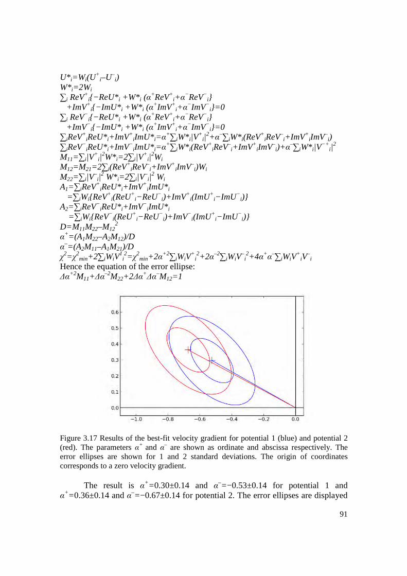
91

U* i=Wi(U+

i–U–i)

W*i=2Wi ∑i ReV+

i−ReU*i +W* i (α+ReV+

i+α−ReV−

i +ImV+

i−ImU* i +W* i (α+ImV+

i+α−ImV−

i=0 ∑i ReV−

i−ReU* i +W* i (α+ReV+

i+α−ReV−

i +ImV−

i−ImU* i +W* i (α+ImV+

i+α−ImV−

i=0 ∑iReV+

iReU*i+ImV+iImU* i=α

+∑iW*i|V+

i|2+α–∑iW*i(ReV+

iReV–i+ImV+

iImV–i)

∑iReV−iReU*i+ImV−

iImU* i=α+∑iW*i(ReV+

iReV–i+ImV+

iImV–i)+α

–∑iW*i|V−+

i|2

M11=∑i|V+

i|2W*i=2∑i|V

+i|

2Wi M12=M21=2∑i(ReV+

iReV–i+ImV+

iImV–i)Wi

M22=∑i|V–i|

2 W*i=2∑i|V–i|

2 Wi A1=∑iReV+

iReU*i+ImV+iImU* i

=∑iWiReV+i(ReU+

i−ReU−i)+ImV+

i(ImU+i−ImU−

i) A2=∑ iReV−

iReU*i+ImV−iImU* i

=∑iWiReV−i(ReU+

i−ReU−i)+ImV−

i(ImU+i−ImU−

i) D=M11M22–M12

2 α+=(A1M22–A2M12)/D α–=(A2M11–A1M21)/D χ2=χ2

min+2∑iWiV1i2=χ2

min+2α+2∑iWiV+

i2+2α–2∑iWiV

–i2+4α+α–∑iWiV

+iV

–i

Hence the equation of the error ellipse: ∆α+2M11+∆α

–2M22+2∆α+∆α–M12=1

Figure 3.17 Results of the best-fit velocity gradient for potential 1 (blue) and potential 2 (red). The parameters α+ and α– are shown as ordinate and abscissa respectively. The error ellipses are shown for 1 and 2 standard deviations. The origin of coordinates corresponds to a zero velocity gradient.

The result is α+=0.30±0.14 and α–=−0.53±0.14 for potential 1 and α+=0.36±0.14 and α–=−0.67±0.14 for potential 2. The error ellipses are displayed

92

in Figure 3.17. The evidence for a velocity gradient is at the level of 3.9 standard deviations for potential 1 and 5.0 standard deviations for potential 2. Combining the two results gives α+=0.33±0.14 and α–=−0.60±0.14, 4.5 standard deviations away from zero. Figure 3.18 displays the sky maps of the observed and predicted images of the eastern and western halves of the source and of the blue and red parts of the line.

Figure 3.18 Sky maps of the observed blue and red parts of the line (left panel). Right panels: predicted images of the eastern and western halves of the source (potential 1 in the middle, potential 2 on the right).

3.8 Continuum In Section 3.4, we estimated ρ=19±9 mas in the continuum, meaning that

the source is only resolved at the level of 2 standard deviations. It is therefore unreasonable to attempt making as detailed studies in the continuum as were done

Figure 3.19 Continuum: dependence of the best-fit χ2 on the source size ρ (mas) for potential 1 (blue) and potential 2 (red) using the best-fit source brightness distribution that has been obtained on the line.

(arcsec)

(arc

sec

)

ρ (mas)

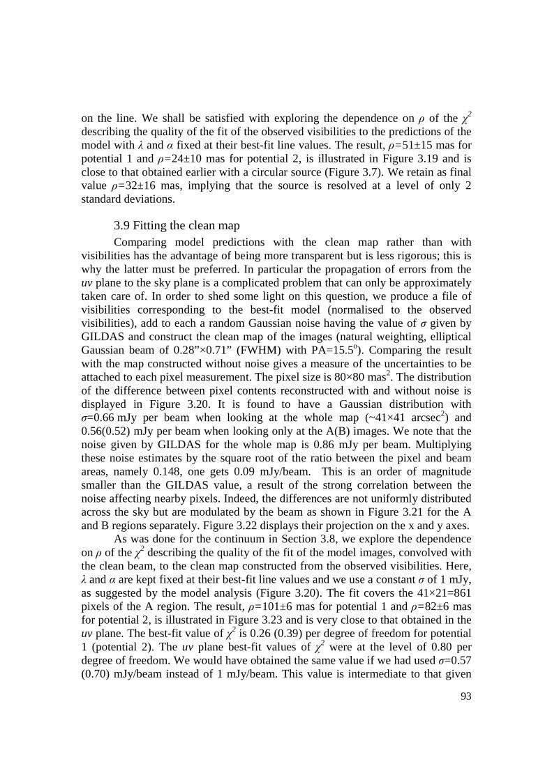
93

on the line. We shall be satisfied with exploring the dependence on ρ of the χ2 describing the quality of the fit of the observed visibilities to the predictions of the model with λ and α fixed at their best-fit line values. The result, ρ=51±15 mas for potential 1 and ρ=24±10 mas for potential 2, is illustrated in Figure 3.19 and is close to that obtained earlier with a circular source (Figure 3.7). We retain as final value ρ=32±16 mas, implying that the source is resolved at a level of only 2 standard deviations.

3.9 Fitting the clean map Comparing model predictions with the clean map rather than with

visibilities has the advantage of being more transparent but is less rigorous; this is why the latter must be preferred. In particular the propagation of errors from the uv plane to the sky plane is a complicated problem that can only be approximately taken care of. In order to shed some light on this question, we produce a file of visibilities corresponding to the best-fit model (normalised to the observed visibilities), add to each a random Gaussian noise having the value of σ given by GILDAS and construct the clean map of the images (natural weighting, elliptical Gaussian beam of 0.28”×0.71” (FWHM) with PA=15.5o). Comparing the result with the map constructed without noise gives a measure of the uncertainties to be attached to each pixel measurement. The pixel size is 80×80 mas2. The distribution of the difference between pixel contents reconstructed with and without noise is displayed in Figure 3.20. It is found to have a Gaussian distribution with σ=0.66 mJy per beam when looking at the whole map (~41×41 arcsec2) and 0.56(0.52) mJy per beam when looking only at the A(B) images. We note that the noise given by GILDAS for the whole map is 0.86 mJy per beam. Multiplying these noise estimates by the square root of the ratio between the pixel and beam areas, namely 0.148, one gets 0.09 mJy/beam. This is an order of magnitude smaller than the GILDAS value, a result of the strong correlation between the noise affecting nearby pixels. Indeed, the differences are not uniformly distributed across the sky but are modulated by the beam as shown in Figure 3.21 for the A and B regions separately. Figure 3.22 displays their projection on the x and y axes.

As was done for the continuum in Section 3.8, we explore the dependence on ρ of the χ2 describing the quality of the fit of the model images, convolved with the clean beam, to the clean map constructed from the observed visibilities. Here, λ and α are kept fixed at their best-fit line values and we use a constant σ of 1 mJy, as suggested by the model analysis (Figure 3.20). The fit covers the 41×21=861 pixels of the A region. The result, ρ=101±6 mas for potential 1 and ρ=82±6 mas for potential 2, is illustrated in Figure 3.23 and is very close to that obtained in the uv plane. The best-fit value of χ2 is 0.26 (0.39) per degree of freedom for potential 1 (potential 2). The uv plane best-fit values of χ2 were at the level of 0.80 per degree of freedom. We would have obtained the same value if we had used σ=0.57 (0.70) mJy/beam instead of 1 mJy/beam. This value is intermediate to that given

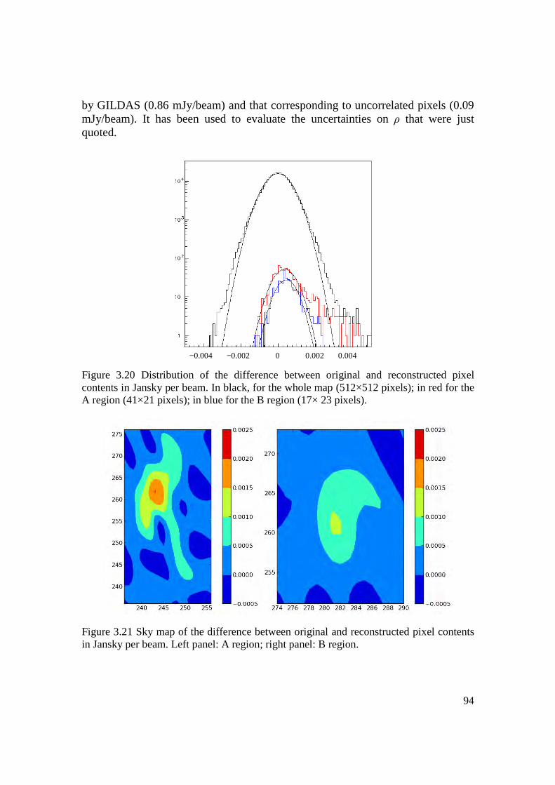
94

by GILDAS (0.86 mJy/beam) and that corresponding to uncorrelated pixels (0.09 mJy/beam). It has been used to evaluate the uncertainties on ρ that were just quoted.

Figure 3.20 Distribution of the difference between original and reconstructed pixel contents in Jansky per beam. In black, for the whole map (512×512 pixels); in red for the A region (41×21 pixels); in blue for the B region (17× 23 pixels).

Figure 3.21 Sky map of the difference between original and reconstructed pixel contents in Jansky per beam. Left panel: A region; right panel: B region.

−0.004 −0.002 0 0.002 0.004

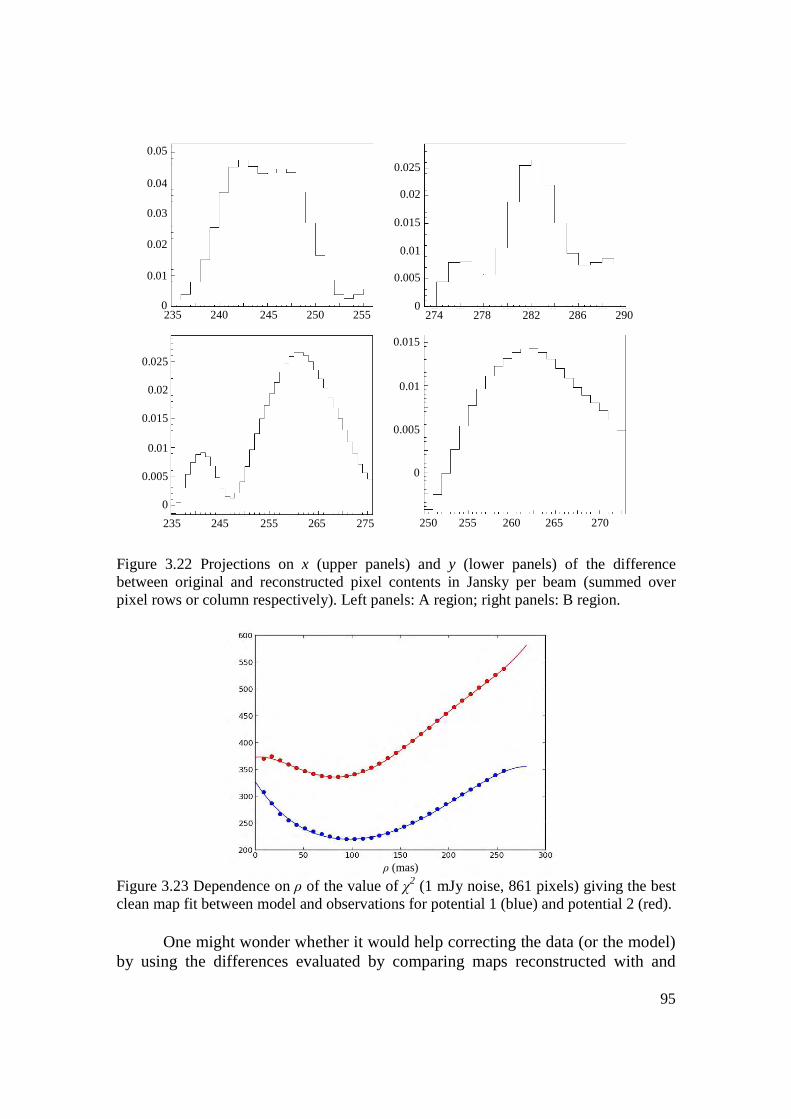
95

Figure 3.22 Projections on x (upper panels) and y (lower panels) of the difference between original and reconstructed pixel contents in Jansky per beam (summed over pixel rows or column respectively). Left panels: A region; right panels: B region.

Figure 3.23 Dependence on ρ of the value of χ2 (1 mJy noise, 861 pixels) giving the best clean map fit between model and observations for potential 1 (blue) and potential 2 (red).

One might wonder whether it would help correcting the data (or the model)

by using the differences evaluated by comparing maps reconstructed with and

274 278 282 286 290 235 240 245 250 255

0.05

0.04

0.03

0.02

0.01

0

0.025

0.02

0.015

0.01

0.005

0

0.025

0.02

0.015

0.01

0.005

0

235 245 255 265 275 250 255 260 265 270

0.015

0.01

0.005

0

ρ (mas)

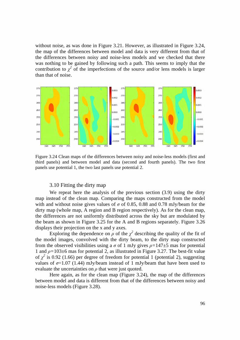
96

without noise, as was done in Figure 3.21. However, as illustrated in Figure 3.24, the map of the differences between model and data is very different from that of the differences between noisy and noise-less models and we checked that there was nothing to be gained by following such a path. This seems to imply that the contribution to χ2 of the imperfections of the source and/or lens models is larger than that of noise.

Figure 3.24 Clean maps of the differences between noisy and noise-less models (first and third panels) and between model and data (second and fourth panels). The two first panels use potential 1, the two last panels use potential 2.

3.10 Fitting the dirty map We repeat here the analysis of the previous section (3.9) using the dirty

map instead of the clean map. Comparing the maps constructed from the model with and without noise gives values of σ of 0.85, 0.88 and 0.78 mJy/beam for the dirty map (whole map, A region and B region respectively). As for the clean map, the differences are not uniformly distributed across the sky but are modulated by the beam as shown in Figure 3.25 for the A and B regions separately. Figure 3.26 displays their projection on the x and y axes.

Exploring the dependence on ρ of the χ2 describing the quality of the fit of the model images, convolved with the dirty beam, to the dirty map constructed from the observed visibilities using a σ of 1 mJy gives ρ=147±5 mas for potential 1 and ρ=103±6 mas for potential 2, as illustrated in Figure 3.27. The best-fit value of χ2 is 0.92 (1.66) per degree of freedom for potential 1 (potential 2), suggesting values of σ=1.07 (1.44) mJy/beam instead of 1 mJy/beam that have been used to evaluate the uncertainties on ρ that were just quoted.

Here again, as for the clean map (Figure 3.24), the map of the differences between model and data is different from that of the differences between noisy and noise-less models (Figure 3.28).

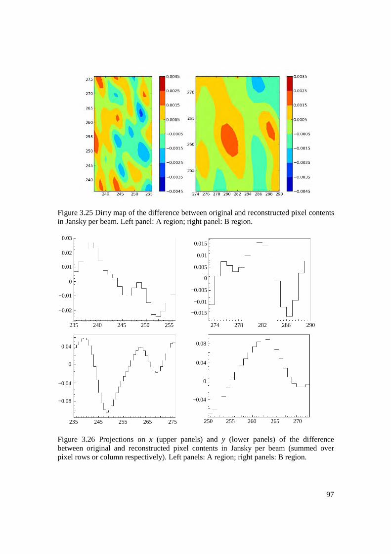
97

Figure 3.25 Dirty map of the difference between original and reconstructed pixel contents in Jansky per beam. Left panel: A region; right panel: B region.

Figure 3.26 Projections on x (upper panels) and y (lower panels) of the difference between original and reconstructed pixel contents in Jansky per beam (summed over pixel rows or column respectively). Left panels: A region; right panels: B region.

274 278 282 286 290

0.03

0.02

0.01

0

−0.01

−0.02

250 255 260 265 270

235 240 245 250 255

235 245 255 265 275

0.04

0

−0.04

−0.08

0.08

0.04

0

−0.04

0.015

0.01

0.005

0

−0.005

−0.01

−0.015

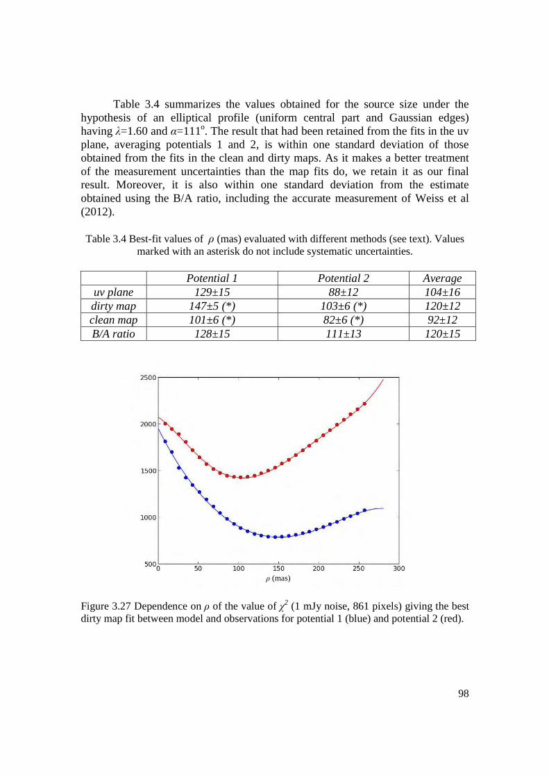
98

Table 3.4 summarizes the values obtained for the source size under the hypothesis of an elliptical profile (uniform central part and Gaussian edges) having λ=1.60 and α=111o. The result that had been retained from the fits in the uv plane, averaging potentials 1 and 2, is within one standard deviation of those obtained from the fits in the clean and dirty maps. As it makes a better treatment of the measurement uncertainties than the map fits do, we retain it as our final result. Moreover, it is also within one standard deviation from the estimate obtained using the B/A ratio, including the accurate measurement of Weiss et al (2012).

Table 3.4 Best-fit values of ρ (mas) evaluated with different methods (see text). Values

marked with an asterisk do not include systematic uncertainties. Potential 1 Potential 2 Average

uv plane 129±15 88±12 104±16 dirty map 147±5 (*) 103±6 (*) 120±12 clean map 101±6 (*) 82±6 (*) 92±12 B/A ratio 128±15 111±13 120±15

Figure 3.27 Dependence on ρ of the value of χ2 (1 mJy noise, 861 pixels) giving the best dirty map fit between model and observations for potential 1 (blue) and potential 2 (red).

ρ (mas)

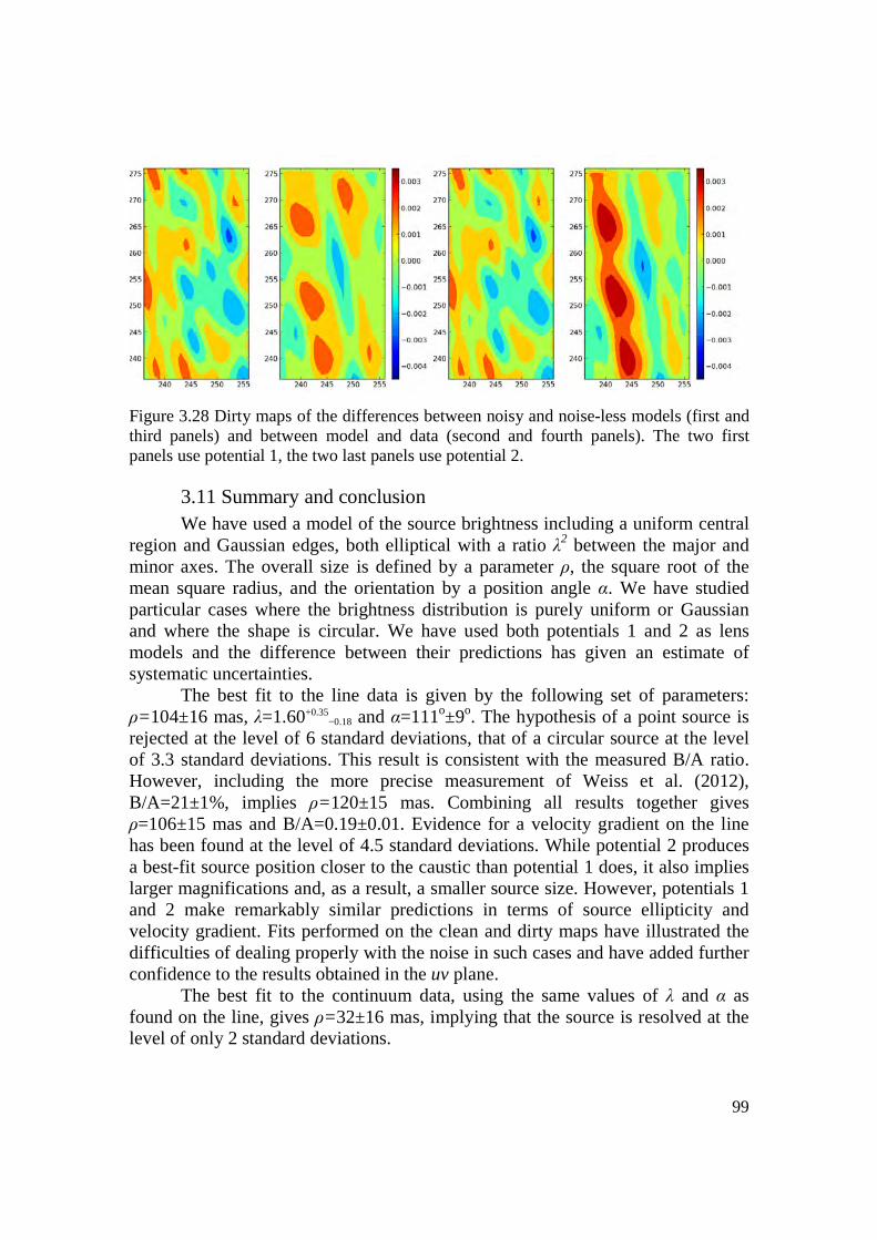
99

Figure 3.28 Dirty maps of the differences between noisy and noise-less models (first and third panels) and between model and data (second and fourth panels). The two first panels use potential 1, the two last panels use potential 2.

3.11 Summary and conclusion We have used a model of the source brightness including a uniform central

region and Gaussian edges, both elliptical with a ratio λ2 between the major and minor axes. The overall size is defined by a parameter ρ, the square root of the mean square radius, and the orientation by a position angle α. We have studied particular cases where the brightness distribution is purely uniform or Gaussian and where the shape is circular. We have used both potentials 1 and 2 as lens models and the difference between their predictions has given an estimate of systematic uncertainties.

The best fit to the line data is given by the following set of parameters: ρ=104±16 mas, λ=1.60+0.35

−0.18 and α=111o±9o. The hypothesis of a point source is rejected at the level of 6 standard deviations, that of a circular source at the level of 3.3 standard deviations. This result is consistent with the measured B/A ratio. However, including the more precise measurement of Weiss et al. (2012), B/A=21±1%, implies ρ=120±15 mas. Combining all results together gives ρ=106±15 mas and B/A=0.19±0.01. Evidence for a velocity gradient on the line has been found at the level of 4.5 standard deviations. While potential 2 produces a best-fit source position closer to the caustic than potential 1 does, it also implies larger magnifications and, as a result, a smaller source size. However, potentials 1 and 2 make remarkably similar predictions in terms of source ellipticity and velocity gradient. Fits performed on the clean and dirty maps have illustrated the difficulties of dealing properly with the noise in such cases and have added further confidence to the results obtained in the uv plane.

The best fit to the continuum data, using the same values of λ and α as found on the line, gives ρ=32±16 mas, implying that the source is resolved at the level of only 2 standard deviations.

100

4. Interpretation of the results

4.1 Galaxy formation and evolution: an introduction 4.1.1 Generalities The observations presented in the preceding sections need to be placed in

the general context of our current understanding of the formation and evolution of galaxies in the early Universe.

Many different families of galaxies have been defined throughout the recent history of astrophysics, in relation with the way they have been discovered and subsequently observed. Most of these are understood today to be equivalent, or at least to broadly overlap, and do not need to be mentioned in the present review, for the purpose of which it is sufficient to distinguish between star-forming galaxies and star-not-forming galaxies. The former are typically blue, dense and dusty spirals including a thin fast rotating disk with young stars, a bulge (possibly barred), and a halo containing low metallicity stars (e.g, Gilmore & Reid 1983; Gilmore, Wyse, & Kuijken 1989, Barnes & Hernquist 1992, Preston, Beers, & Shectman 1994). The latter are typically red ellipticals, made of old stars and containing little to no dust (e.g, Martig et al. 2009, Young et al. 2011). Both types usually have a black hole in their centre, with masses ranging from a few millions to a few billions solar masses, and are contained in large dark matter haloes, the more so the more massive they are (e.g, Gultekin et al. 2009).

Many galaxies in the universe are gravitationally bound to other galaxies and interact. Encounters have consequences that depend strongly on the impact parameter and the mass ratio of the interacting galaxies. They often result in mergers that play an important role in the evolution of structures in the Universe. Minor mergers of a spiral and a galaxy having a mass at least an order of magnitude smaller, say a dwarf, simply disturb the morphology of the spiral by wrapping the disk and making the bulge thicker and hotter (e.g, Walker, Mihos & Hernquist 1996). Such an example is illustrated in Figure 4.1. Major mergers between two spirals, the mass of the smaller exceeding a third or so of the mass of the larger destroy the disk morphology and produce a strong dispersion and relaxation effect, the final product being an elliptical galaxy (e.g, Negroponte& White 1983; Barnes 1998; Naab & Burkert 2003).

Massive elliptical galaxies have a supermassive black hole (SMBH) in their centre. They stand out in the M-σ diagram (Figure 4.2) that relates the mass M of the black hole to the velocity dispersion σ. A power law is expected, of the form M α σγ for a Keplerian disk or for a virialized volume, implying a similar law when replacing the mass M by luminosity L (Tully-Fisher for spirals, Faber-Jackson for ellipticals). Figure 4.2 is for the bulge and implies that the mass of the central black hole is roughly proportional to that of the bulge, MBH~0.2% M(bulge).

101

Figure 4.1 A spiral, ESO 510-G13, warped by a collision with another galaxy (Credit: NASA and The Hubble Heritage Team STscl/AURA).

Figure 4.2 M-σ relation displaying the mass of the central black hole as a function of the dispersion of the star velocities in the bulge. The left panel (see e.g, Ferrarese & Merritt 2000) is for spirals selected for galaxies which exhibit a clear, Keplerian rise in velocity near the centre while the right panel (Gultekin et al. 2009) distinguishes between ellipticals (red) and spirals (blue).

Galaxies are distributed in a great cosmic web of filaments throughout the

Universe. The locations where the filaments meet are dense clusters of galaxies that began as small fluctuations in the early universe. Hence the distribution of galaxies is closely related to the physics of the early Universe. Simulations reproduce the clustering of dark matter preceding that of gas (H and He) and galaxies growing by accreting smaller galaxies while the dark matter stays mostly on their outer parts. They successfully predict the presence of large voids, with densities ~1/10 the cosmological mean. Matter condenses in large filaments

As massive as today’s

largest SMBHs but

when Universe was <

1Gyr old

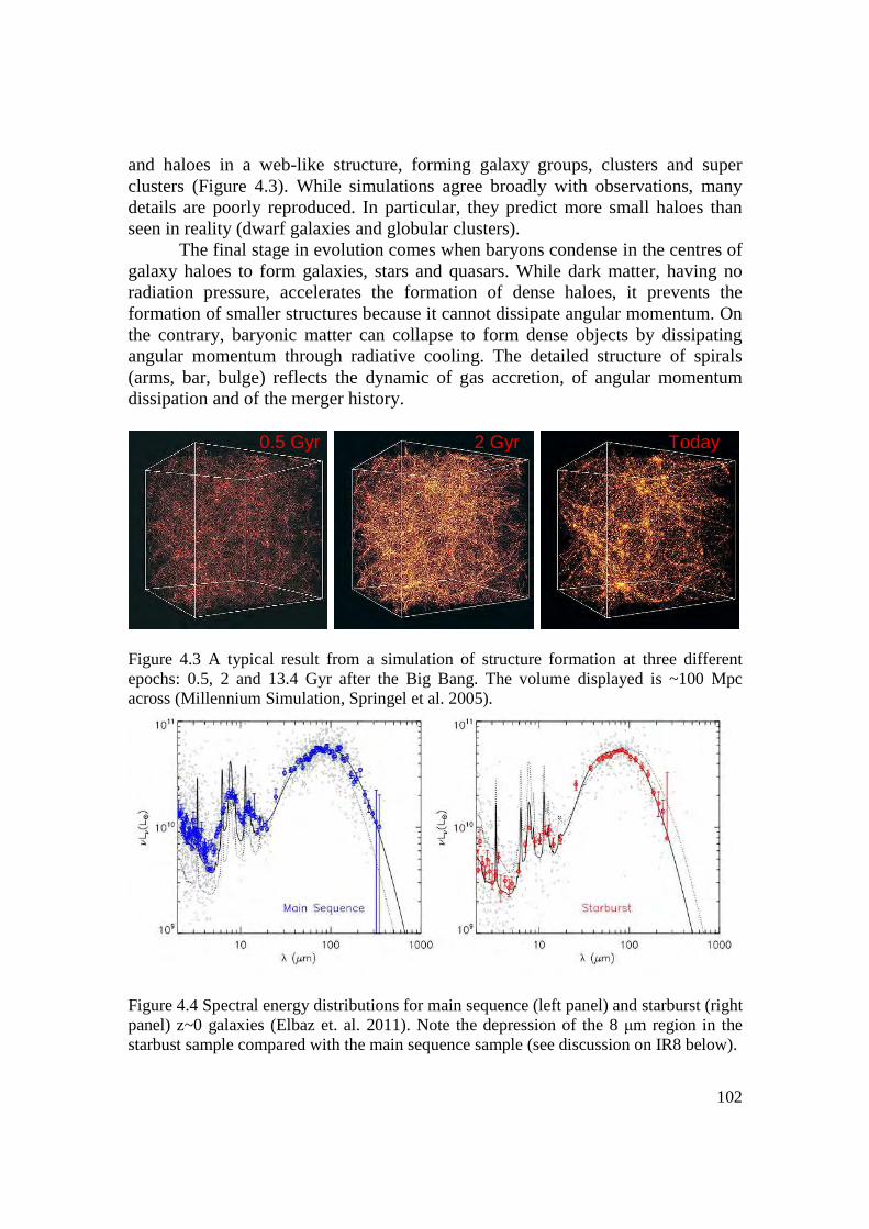
102

and haloes in a web-like structure, forming galaxy groups, clusters and super clusters (Figure 4.3). While simulations agree broadly with observations, many details are poorly reproduced. In particular, they predict more small haloes than seen in reality (dwarf galaxies and globular clusters).

The final stage in evolution comes when baryons condense in the centres of galaxy haloes to form galaxies, stars and quasars. While dark matter, having no radiation pressure, accelerates the formation of dense haloes, it prevents the formation of smaller structures because it cannot dissipate angular momentum. On the contrary, baryonic matter can collapse to form dense objects by dissipating angular momentum through radiative cooling. The detailed structure of spirals (arms, bar, bulge) reflects the dynamic of gas accretion, of angular momentum dissipation and of the merger history.

Figure 4.3 A typical result from a simulation of structure formation at three different epochs: 0.5, 2 and 13.4 Gyr after the Big Bang. The volume displayed is ~100 Mpc across (Millennium Simulation, Springel et al. 2005).

Figure 4.4 Spectral energy distributions for main sequence (left panel) and starburst (right panel) z~0 galaxies (Elbaz et. al. 2011). Note the depression of the 8 µm region in the starbust sample compared with the main sequence sample (see discussion on IR8 below).

0.5 Gyr 2 Gyr Today

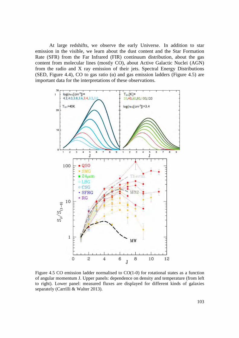
103

At large redshifts, we observe the early Universe. In addition to star emission in the visible, we learn about the dust content and the Star Formation Rate (SFR) from the Far Infrared (FIR) continuum distribution, about the gas content from molecular lines (mostly CO), about Active Galactic Nuclei (AGN) from the radio and X ray emission of their jets. Spectral Energy Distributions (SED, Figure 4.4), CO to gas ratio (α) and gas emission ladders (Figure 4.5) are important data for the interpretations of these observations.

Figure 4.5 CO emission ladder normalised to CO(1-0) for rotational states as a function of angular momentum J. Upper panels: dependence on density and temperature (from left to right). Lower panel: measured fluxes are displayed for different kinds of galaxies separately (Carrilli & Walter 2013).

−10−2

−10−2

ρ (mas)

number images

(arcsec)

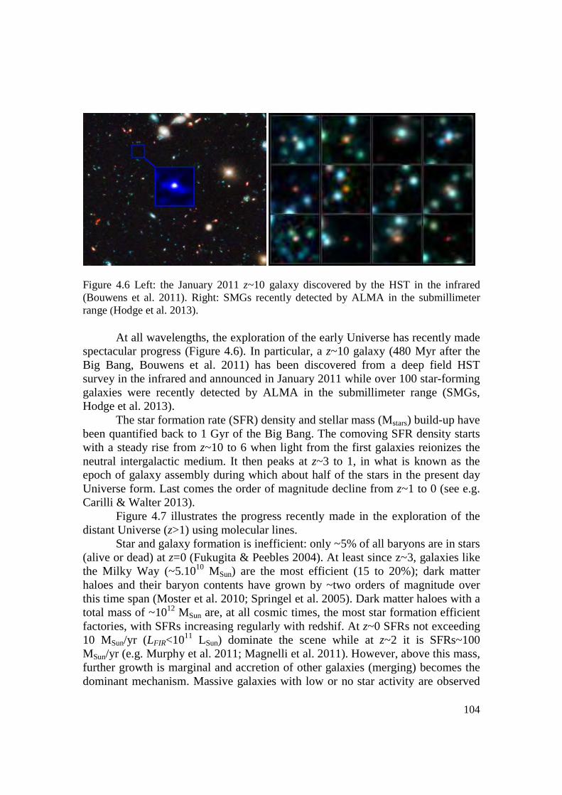
104

Figure 4.6 Left: the January 2011 z~10 galaxy discovered by the HST in the infrared (Bouwens et al. 2011). Right: SMGs recently detected by ALMA in the submillimeter range (Hodge et al. 2013).

At all wavelengths, the exploration of the early Universe has recently made spectacular progress (Figure 4.6). In particular, a z~10 galaxy (480 Myr after the Big Bang, Bouwens et al. 2011) has been discovered from a deep field HST survey in the infrared and announced in January 2011 while over 100 star-forming galaxies were recently detected by ALMA in the submillimeter range (SMGs, Hodge et al. 2013).

The star formation rate (SFR) density and stellar mass (Mstars) build-up have been quantified back to 1 Gyr of the Big Bang. The comoving SFR density starts with a steady rise from z~10 to 6 when light from the first galaxies reionizes the neutral intergalactic medium. It then peaks at z~3 to 1, in what is known as the epoch of galaxy assembly during which about half of the stars in the present day Universe form. Last comes the order of magnitude decline from z~1 to 0 (see e.g. Carilli & Walter 2013).

Figure 4.7 illustrates the progress recently made in the exploration of the distant Universe (z>1) using molecular lines.

Star and galaxy formation is inefficient: only ~5% of all baryons are in stars (alive or dead) at z=0 (Fukugita & Peebles 2004). At least since z~3, galaxies like the Milky Way (~5.1010 MSun) are the most efficient (15 to 20%); dark matter haloes and their baryon contents have grown by ~two orders of magnitude over this time span (Moster et al. 2010; Springel et al. 2005). Dark matter haloes with a total mass of ~1012 MSun are, at all cosmic times, the most star formation efficient factories, with SFRs increasing regularly with redshif. At z~0 SFRs not exceeding 10 MSun/yr (LFIR<1011 LSun) dominate the scene while at z~2 it is SFRs~100 MSun/yr (e.g. Murphy et al. 2011; Magnelli et al. 2011). However, above this mass, further growth is marginal and accretion of other galaxies (merging) becomes the dominant mechanism. Massive galaxies with low or no star activity are observed

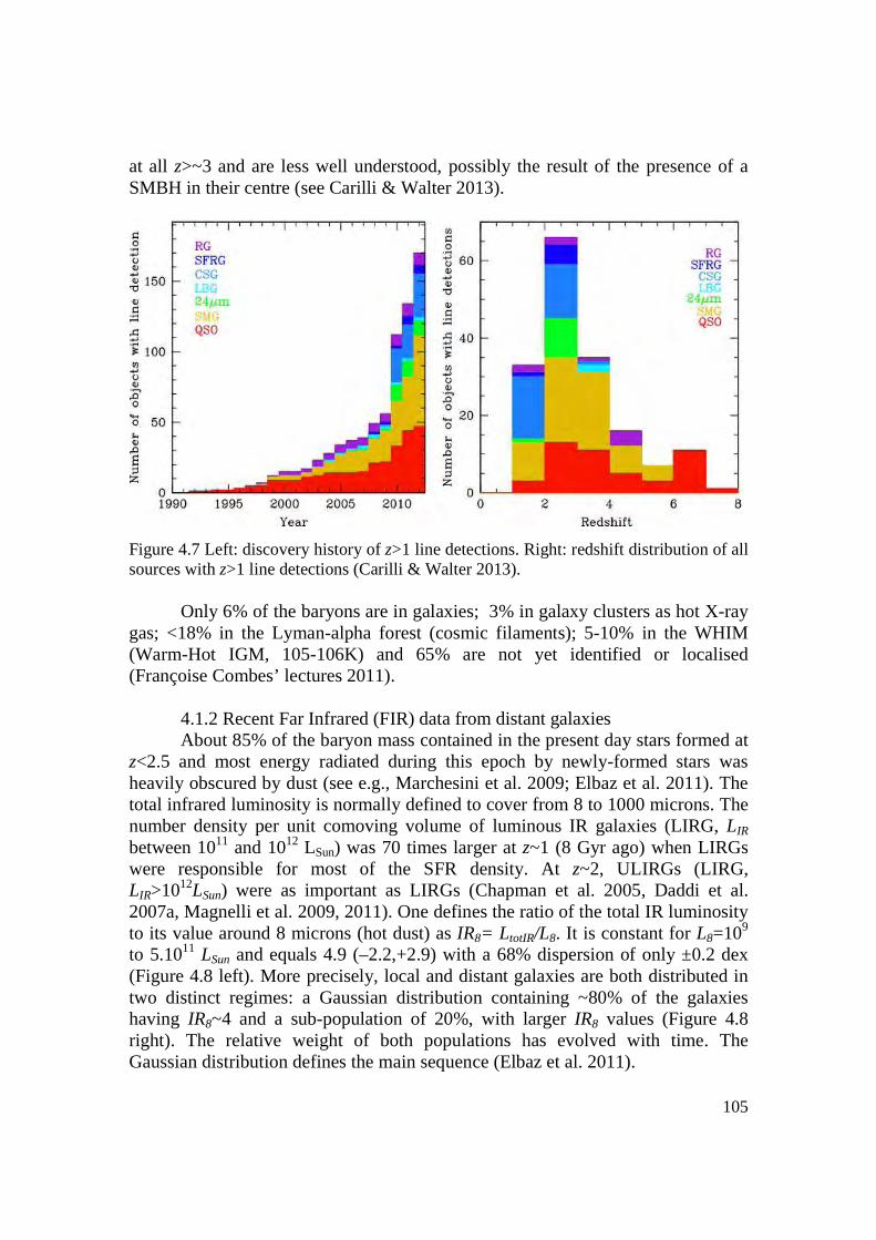
105

at all z>~3 and are less well understood, possibly the result of the presence of a SMBH in their centre (see Carilli & Walter 2013).

Figure 4.7 Left: discovery history of z>1 line detections. Right: redshift distribution of all sources with z>1 line detections (Carilli & Walter 2013).

Only 6% of the baryons are in galaxies; 3% in galaxy clusters as hot X-ray

gas; <18% in the Lyman-alpha forest (cosmic filaments); 5-10% in the WHIM (Warm-Hot IGM, 105-106K) and 65% are not yet identified or localised (Françoise Combes’ lectures 2011).

4.1.2 Recent Far Infrared (FIR) data from distant galaxies About 85% of the baryon mass contained in the present day stars formed at

z<2.5 and most energy radiated during this epoch by newly-formed stars was heavily obscured by dust (see e.g., Marchesini et al. 2009; Elbaz et al. 2011). The total infrared luminosity is normally defined to cover from 8 to 1000 microns. The number density per unit comoving volume of luminous IR galaxies (LIRG, LIR between 1011 and 1012 LSun) was 70 times larger at z~1 (8 Gyr ago) when LIRGs were responsible for most of the SFR density. At z~2, ULIRGs (LIRG, LIR>1012LSun) were as important as LIRGs (Chapman et al. 2005, Daddi et al. 2007a, Magnelli et al. 2009, 2011). One defines the ratio of the total IR luminosity to its value around 8 microns (hot dust) as IR8= L totIR/L8. It is constant for L8=109 to 5.1011 LSun and equals 4.9 (–2.2,+2.9) with a 68% dispersion of only ±0.2 dex (Figure 4.8 left). More precisely, local and distant galaxies are both distributed in two distinct regimes: a Gaussian distribution containing ~80% of the galaxies having IR8~4 and a sub-population of 20%, with larger IR8 values (Figure 4.8 right). The relative weight of both populations has evolved with time. The Gaussian distribution defines the main sequence (Elbaz et al. 2011).

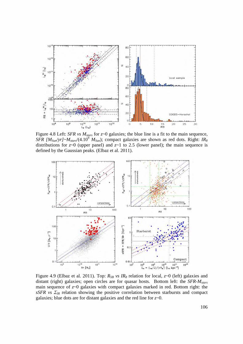
106

Figure 4.8 Left: SFR vs Mstars for z~0 galaxies; the blue line is a fit to the main sequence, SFR [MSun/yr]~Mstars/(4.109 MSun); compact galaxies are shown as red dots. Right: IR8 distributions for z~0 (upper panel) and z~1 to 2.5 (lower panel); the main sequence is defined by the Gaussian peaks. (Elbaz et al. 2011).

Figure 4.9 (Elbaz et al. 2011). Top: RSB vs IR8 relation for local, z~0 (left) galaxies and distant (right) galaxies; open circles are for quasar hosts. Bottom left: the SFR-Mstars main sequence of z~0 galaxies with compact galaxies marked in red. Bottom right: the sSFR vs ΣIR relation showing the positive correlation between starbursts and compact galaxies; blue dots are for distant galaxies and the red line for z~0.

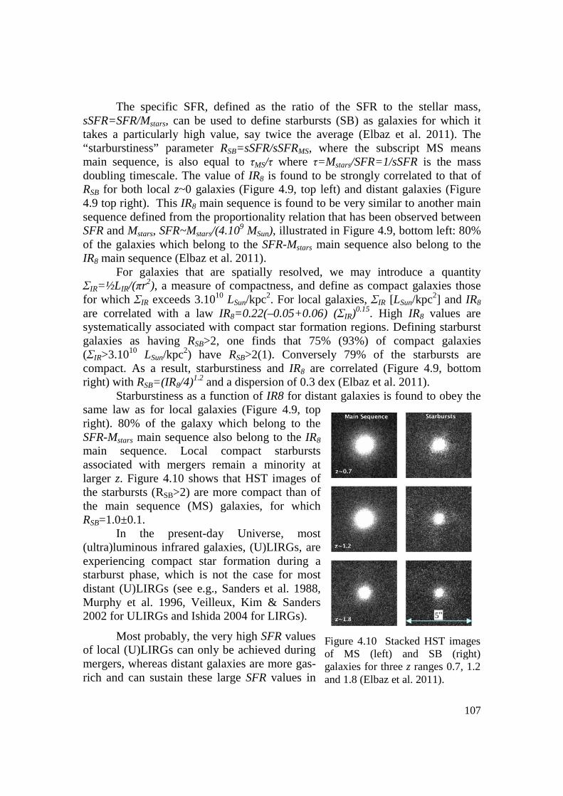
107

The specific SFR, defined as the ratio of the SFR to the stellar mass, sSFR=SFR/Mstars, can be used to define starbursts (SB) as galaxies for which it takes a particularly high value, say twice the average (Elbaz et al. 2011). The “starburstiness” parameter RSB=sSFR/sSFRMS, where the subscript MS means main sequence, is also equal to τMS/τ where τ=Mstars/SFR=1/sSFR is the mass doubling timescale. The value of IR8 is found to be strongly correlated to that of RSB for both local z~0 galaxies (Figure 4.9, top left) and distant galaxies (Figure 4.9 top right). This IR8 main sequence is found to be very similar to another main sequence defined from the proportionality relation that has been observed between SFR and Mstars, SFR~Mstars/(4.109 MSun), illustrated in Figure 4.9, bottom left: 80% of the galaxies which belong to the SFR-Mstars main sequence also belong to the IR8 main sequence (Elbaz et al. 2011).

For galaxies that are spatially resolved, we may introduce a quantity ΣIR=½LIR/(πr2), a measure of compactness, and define as compact galaxies those for which ΣIR exceeds 3.1010 LSun/kpc2. For local galaxies, ΣIR [LSun/kpc2] and IR8 are correlated with a law IR8=0.22(–0.05+0.06) (ΣIR)0.15. High IR8 values are systematically associated with compact star formation regions. Defining starburst galaxies as having RSB>2, one finds that 75% (93%) of compact galaxies (ΣIR>3.1010 LSun/kpc2) have RSB>2(1). Conversely 79% of the starbursts are compact. As a result, starburstiness and IR8 are correlated (Figure 4.9, bottom right) with RSB=(IR8/4)1.2 and a dispersion of 0.3 dex (Elbaz et al. 2011).

Starburstiness as a function of IR8 for distant galaxies is found to obey the same law as for local galaxies (Figure 4.9, top right). 80% of the galaxy which belong to the SFR-Mstars main sequence also belong to the IR8 main sequence. Local compact starbursts associated with mergers remain a minority at larger z. Figure 4.10 shows that HST images of the starbursts (RSB>2) are more compact than of the main sequence (MS) galaxies, for which RSB=1.0±0.1.

In the present-day Universe, most (ultra)luminous infrared galaxies, (U)LIRGs, are experiencing compact star formation during a starburst phase, which is not the case for most distant (U)LIRGs (see e.g., Sanders et al. 1988, Murphy et al. 1996, Veilleux, Kim & Sanders 2002 for ULIRGs and Ishida 2004 for LIRGs).

Most probably, the very high SFR values of local (U)LIRGs can only be achieved during mergers, whereas distant galaxies are more gas-rich and can sustain these large SFR values in

Figure 4.10 Stacked HST images of MS (left) and SB (right) galaxies for three z ranges 0.7, 1.2 and 1.8 (Elbaz et al. 2011).

5''

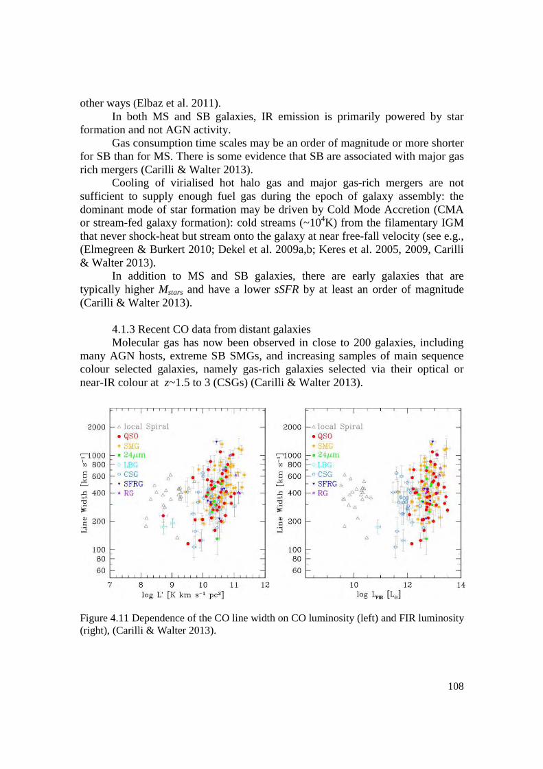
108

other ways (Elbaz et al. 2011). In both MS and SB galaxies, IR emission is primarily powered by star

formation and not AGN activity. Gas consumption time scales may be an order of magnitude or more shorter

for SB than for MS. There is some evidence that SB are associated with major gas rich mergers (Carilli & Walter 2013).

Cooling of virialised hot halo gas and major gas-rich mergers are not sufficient to supply enough fuel gas during the epoch of galaxy assembly: the dominant mode of star formation may be driven by Cold Mode Accretion (CMA or stream-fed galaxy formation): cold streams (~104K) from the filamentary IGM that never shock-heat but stream onto the galaxy at near free-fall velocity (see e.g., (Elmegreen & Burkert 2010; Dekel et al. 2009a,b; Keres et al. 2005, 2009, Carilli & Walter 2013).

In addition to MS and SB galaxies, there are early galaxies that are typically higher Mstars and have a lower sSFR by at least an order of magnitude (Carilli & Walter 2013).

4.1.3 Recent CO data from distant galaxies Molecular gas has now been observed in close to 200 galaxies, including

many AGN hosts, extreme SB SMGs, and increasing samples of main sequence colour selected galaxies, namely gas-rich galaxies selected via their optical or near-IR colour at z~1.5 to 3 (CSGs) (Carilli & Walter 2013).

Figure 4.11 Dependence of the CO line width on CO luminosity (left) and FIR luminosity (right), (Carilli & Walter 2013).

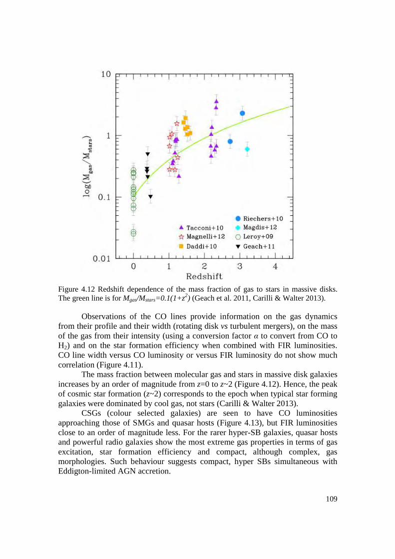
109

Figure 4.12 Redshift dependence of the mass fraction of gas to stars in massive disks. The green line is for Mgas/Mstars=0.1(1+z2) (Geach et al. 2011, Carilli & Walter 2013).

Observations of the CO lines provide information on the gas dynamics from their profile and their width (rotating disk vs turbulent mergers), on the mass of the gas from their intensity (using a conversion factor α to convert from CO to H2) and on the star formation efficiency when combined with FIR luminosities. CO line width versus CO luminosity or versus FIR luminosity do not show much correlation (Figure 4.11).

The mass fraction between molecular gas and stars in massive disk galaxies increases by an order of magnitude from z=0 to z~2 (Figure 4.12). Hence, the peak of cosmic star formation (z~2) corresponds to the epoch when typical star forming galaxies were dominated by cool gas, not stars (Carilli & Walter 2013).

CSGs (colour selected galaxies) are seen to have CO luminosities approaching those of SMGs and quasar hosts (Figure 4.13), but FIR luminosities close to an order of magnitude less. For the rarer hyper-SB galaxies, quasar hosts and powerful radio galaxies show the most extreme gas properties in terms of gas excitation, star formation efficiency and compact, although complex, gas morphologies. Such behaviour suggests compact, hyper SBs simultaneous with Eddigton-limited AGN accretion.

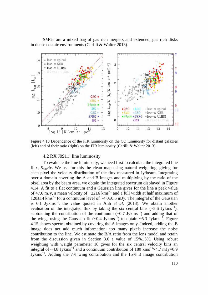
110

SMGs are a mixed bag of gas rich mergers and extended, gas rich disks in dense cosmic environments (Carilli & Walter 2013).

Figure 4.13 Dependence of the FIR luminosity on the CO luminosity for distant galaxies (left) and of their ratio (right) on the FIR luminosity (Carilli & Walter 2013).

4.2 RX J0911: line luminosity To evaluate the line luminosity, we need first to calculate the integrated line

flux, Sline∆ν. We use for this the clean map using natural weighting, giving for each pixel the velocity distribution of the flux measured in Jy/beam. Integrating over a domain covering the A and B images and multiplying by the ratio of the pixel area by the beam area, we obtain the integrated spectrum displayed in Figure 4.14. A fit to a flat continuum and a Gaussian line gives for the line a peak value of 47.6 mJy, a mean velocity of −22±6 kms−1 and a full width at half maximum of 120±14 kms−1 for a continuum level of ~4.0±0.5 mJy. The integral of the Gaussian is 6.1 Jykms−1, the value quoted in Anh et al. (2013). We obtain another evaluation of the integrated flux by taking the six central bins (~5.6 Jykms−1), subtracting the contribution of the continuum (~0.7 Jykms−1) and adding that of the wings using the Gaussian fit (~0.4 Jykms−1) to obtain ~5.3 Jykms−1. Figure 4.15 shows spectra obtained by covering the A images only. Indeed, adding the B image does not add much information: too many pixels increase the noise contribution to the line. We estimate the B/A ratio from the lens model and retain from the discussion given in Section 3.6 a value of 15%±5%. Using robust weighting with weight parameter 10 gives for the six central velocity bins an integral of ~4.8 Jykms−1 and a continuum contribution of 180 kms−1×4.7 mJy=0.9 Jykms−1. Adding the 7% wing contribution and the 15% B image contribution

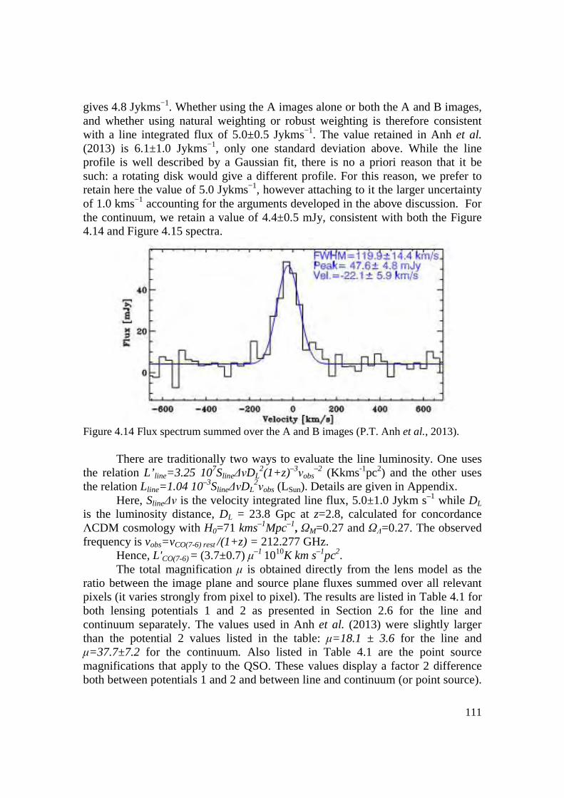
111

gives 4.8 Jykms−1. Whether using the A images alone or both the A and B images, and whether using natural weighting or robust weighting is therefore consistent with a line integrated flux of 5.0±0.5 Jykms−1. The value retained in Anh et al. (2013) is 6.1±1.0 Jykms−1, only one standard deviation above. While the line profile is well described by a Gaussian fit, there is no a priori reason that it be such: a rotating disk would give a different profile. For this reason, we prefer to retain here the value of 5.0 Jykms−1, however attaching to it the larger uncertainty of 1.0 kms−1 accounting for the arguments developed in the above discussion. For the continuum, we retain a value of 4.4±0.5 mJy, consistent with both the Figure 4.14 and Figure 4.15 spectra.

Figure 4.14 Flux spectrum summed over the A and B images (P.T. Anh et al., 2013).

There are traditionally two ways to evaluate the line luminosity. One uses

the relation L’ line=3.25 107Sline∆νDL2(1+z)–3νobs

–2 (Kkms-1pc2) and the other uses the relation Lline=1.04 10–3Sline∆νDL

2νobs (LSun). Details are given in Appendix. Here, Sline∆ν is the velocity integrated line flux, 5.0±1.0 Jykm s–1 while DL

is the luminosity distance, DL = 23.8 Gpc at z=2.8, calculated for concordance ΛCDM cosmology with H0=71 kms–1Mpc–1, ΩM=0.27 and ΩΛ=0.27. The observed frequency is vobs=vCO(7-6) rest /(1+z) = 212.277 GHz.

Hence, L'CO(7-6) = (3.7±0.7) µ–1 1010K km s–1pc2. The total magnification µ is obtained directly from the lens model as the

ratio between the image plane and source plane fluxes summed over all relevant pixels (it varies strongly from pixel to pixel). The results are listed in Table 4.1 for both lensing potentials 1 and 2 as presented in Section 2.6 for the line and continuum separately. The values used in Anh et al. (2013) were slightly larger than the potential 2 values listed in the table: µ=18.1 ± 3.6 for the line and µ=37.7±7.2 for the continuum. Also listed in Table 4.1 are the point source magnifications that apply to the QSO. These values display a factor 2 difference both between potentials 1 and 2 and between line and continuum (or point source).

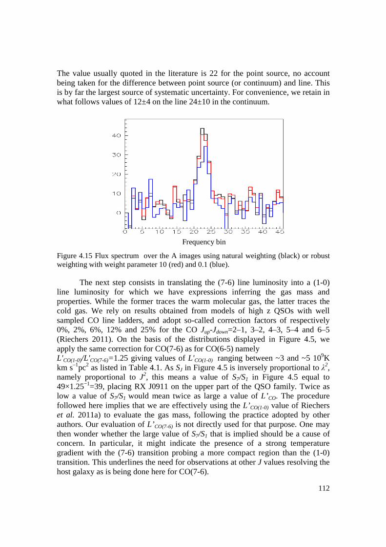
112

The value usually quoted in the literature is 22 for the point source, no account being taken for the difference between point source (or continuum) and line. This is by far the largest source of systematic uncertainty. For convenience, we retain in what follows values of 12±4 on the line 24±10 in the continuum.

Figure 4.15 Flux spectrum over the A images using natural weighting (black) or robust weighting with weight parameter 10 (red) and 0.1 (blue).

The next step consists in translating the (7-6) line luminosity into a (1-0)

line luminosity for which we have expressions inferring the gas mass and properties. While the former traces the warm molecular gas, the latter traces the cold gas. We rely on results obtained from models of high z QSOs with well sampled CO line ladders, and adopt so-called correction factors of respectively 0%, 2%, 6%, 12% and 25% for the CO Jup-Jdown=2–1, 3–2, 4–3, 5–4 and 6–5 (Riechers 2011). On the basis of the distributions displayed in Figure 4.5, we apply the same correction for CO(7-6) as for CO(6-5) namely L'CO(1-0)/L'CO(7-6)=1.25 giving values of L'CO(1-0) ranging between ~3 and ~5 109K km s–1pc2 as listed in Table 4.1. As SJ in Figure 4.5 is inversely proportional to λ2, namely proportional to J2, this means a value of S7/S1 in Figure 4.5 equal to 49×1.25−1=39, placing RX J0911 on the upper part of the QSO family. Twice as low a value of S7/S1 would mean twice as large a value of L’ CO. The procedure followed here implies that we are effectively using the L’CO(1-0) value of Riechers et al. 2011a) to evaluate the gas mass, following the practice adopted by other authors. Our evaluation of L’CO(7-6) is not directly used for that purpose. One may then wonder whether the large value of S7/S1 that is implied should be a cause of concern. In particular, it might indicate the presence of a strong temperature gradient with the (7-6) transition probing a more compact region than the (1-0) transition. This underlines the need for observations at other J values resolving the host galaxy as is being done here for CO(7-6).

Frequency bin

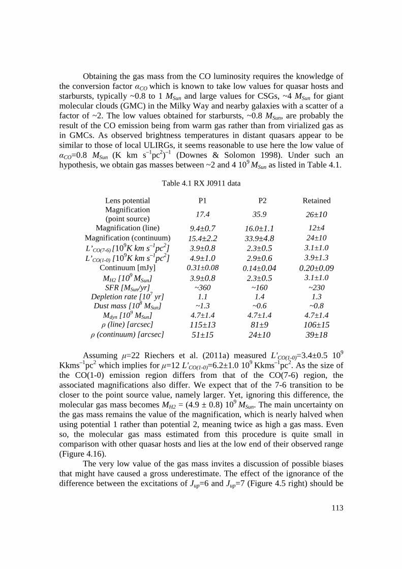
113

Obtaining the gas mass from the CO luminosity requires the knowledge of the conversion factor αCO which is known to take low values for quasar hosts and starbursts, typically ~0.8 to 1 MSun and large values for CSGs, ~4 MSun for giant molecular clouds (GMC) in the Milky Way and nearby galaxies with a scatter of a factor of ~2. The low values obtained for starbursts, ~0.8 MSun, are probably the result of the CO emission being from warm gas rather than from virialized gas as in GMCs. As observed brightness temperatures in distant quasars appear to be similar to those of local ULIRGs, it seems reasonable to use here the low value of αCO=0.8 MSun (K km s–1pc2)–1 (Downes & Solomon 1998). Under such an hypothesis, we obtain gas masses between ~2 and 4 109 MSun as listed in Table 4.1.

Table 4.1 RX J0911 data

Lens potential P1 P2 Retained Magnification (point source)

17.4 35.9 26±10

Magnification (line) 9.4±0.7 16.0±1.1 12±4 Magnification (continuum) 15.4±2.2 33.9±4.8 24±10 L’CO(7-6) [109K km s–1pc2] 3.9±0.8 2.3±0.5 3.1±1.0 L’CO(1-0) [109K km s–1pc2] 4.9±1.0 2.9±0.6 3.9±1.3

Continuum [mJy] 0.31±0.08 0.14±0.04 0.20±0.09 MH2 [109 MSun] 3.9±0.8 2.3±0.5 3.1±1.0 SFR [MSun/yr] ~360 ~160 ~230

Depletion rate [107 yr] 1.1 1.4 1.3 Dust mass [108 MSun] ~1.3 ~0.6 ~0.8

Mdyn [109 MSun] 4.7±1.4 4.7±1.4 4.7±1.4 ρ (line) [arcsec] 115±13 81±9 106±15

ρ (continuum) [arcsec] 51±15 24±10 39±18

Assuming µ=22 Riechers et al. (2011a) measured L'CO(1-0)=3.4±0.5 109

Kkms–1pc2 which implies for µ=12 L'CO(1-0)=6.2±1.0 109 Kkms–1pc2. As the size of the CO(1-0) emission region differs from that of the CO(7-6) region, the associated magnifications also differ. We expect that of the 7-6 transition to be closer to the point source value, namely larger. Yet, ignoring this difference, the molecular gas mass becomes MH2 = (4.9 ± 0.8) 109 MSun. The main uncertainty on the gas mass remains the value of the magnification, which is nearly halved when using potential 1 rather than potential 2, meaning twice as high a gas mass. Even so, the molecular gas mass estimated from this procedure is quite small in comparison with other quasar hosts and lies at the low end of their observed range (Figure 4.16).

The very low value of the gas mass invites a discussion of possible biases that might have caused a gross underestimate. The effect of the ignorance of the difference between the excitations of Jup=6 and Jup=7 (Figure 4.5 right) should be

114

small. In general, one may question the validity of the assumption that the abnormal low values of the gas mass and line width obtained for RX J0911 do not affect the results obtained for typical quasar hosts. In particular, can the CO excitation still be modelled by a single temperature, ~40 to 60 K, and a single

Figure 4.16 Molecular gas mass vs. CO line FWHM for 36 molecular emission line galaxies (EMGs) from Solomon & Vanden Bout 2005, including 15 QSOs (crosses), 7 radio galaxies (diamonds), 12 sub millimeter galaxies (SMGs) (triangles), 1 Extremely red object (ERO) (square), and 1 Lyman break galaxy (LBG) (asterisk). The red bar is for RX J0911 (Table 4.1). All data points are raw data (not corrected for inclination in the hypothesis of a rotating disk).

density, ~103.6 to 4.3 H2/cm3 out to high J values? We mentioned earlier the possible presence of a temperature gradient with the (7-6) transition probing a more compact region than the (1-0) transition. On average, the typical SMG density is log(n(H2)[cm−3])=102.7 to 3.5 H2/cm3 and temperatures are in the range of 30 to 50 K. Quoting from Carilli and Walter (2013), broadly speaking, gas rich quasars and SMGs represent different stages of galaxy evolution, with the quasars being more compact and harbouring more highly excited gas than the SMGs. Yet, even if the low α value adopted here were grossly underestimated, the effect should not exceed a factor 2 or so and the uncertainty on the lensing magnification, another factor of 2, is likely to be the main cause of concern. The low gas mass of RX J0911, when compared with other high-z objects, whether quasar hosts or SMGs, seems therefore to be real.

An excellent review of the state of the art in matters of CO to H2 ratio has been recently published (Bolatto 2013). It underlines the many uncertainties that govern these estimates. Both the CO(7-6) to CO(1-0) ratio and the α factor used to infer the H2 mass rest on relatively shaky hypotheses. The need for more accurate measurements of the line ratio for different J values is blatant. Observing other

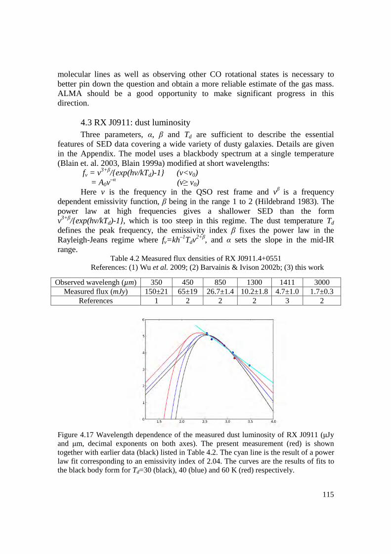
115

molecular lines as well as observing other CO rotational states is necessary to better pin down the question and obtain a more reliable estimate of the gas mass. ALMA should be a good opportunity to make significant progress in this direction.

4.3 RX J0911: dust luminosity Three parameters, α, β and Td are sufficient to describe the essential

features of SED data covering a wide variety of dusty galaxies. Details are given in the Appendix. The model uses a blackbody spectrum at a single temperature (Blain et. al. 2003, Blain 1999a) modified at short wavelengths:

fv = v3+β/exp(hv/kTd)-1 (v<v0) = A0v

–α (v≥ v0) Here v is the frequency in the QSO rest frame and vβ is a frequency

dependent emissivity function, β being in the range 1 to 2 (Hildebrand 1983). The power law at high frequencies gives a shallower SED than the form v3+β/exp(hv/kTd)-1, which is too steep in this regime. The dust temperature Td defines the peak frequency, the emissivity index β fixes the power law in the Rayleigh-Jeans regime where fv=kh–1Tdv

2+β, and α sets the slope in the mid-IR range.

Table 4.2 Measured flux densities of RX J0911.4+0551 References: (1) Wu et al. 2009; (2) Barvainis & Ivison 2002b; (3) this work

Observed wavelengh (µm) 350 450 850 1300 1411 3000 Measured flux (mJy) 150±21 65±19 26.7±1.4 10.2±1.8 4.7±1.0 1.7±0.3

References 1 2 2 2 3 2

Figure 4.17 Wavelength dependence of the measured dust luminosity of RX J0911 (µJy and µm, decimal exponents on both axes). The present measurement (red) is shown together with earlier data (black) listed in Table 4.2. The cyan line is the result of a power law fit corresponding to an emissivity index of 2.04. The curves are the results of fits to the black body form for Td=30 (black), 40 (blue) and 60 K (red) respectively.

116

In the case of RX J0911.4+0551, Table 4.2 lists, and Figure 4.17 displays the data available to evaluate the SED. They include the present measurement at 212.5 GHz, with a flux density of 4.7±1.0 µ–1 mJy. As the value of the magnification is the same for all data, the µ–1 factor is ignored in the figure: it is the shape of the distribution, and not its absolute value, that matters to evaluate Td and β. All available data being in the Rayleigh-Jeans region, they do not allow a determination of α which is therefore irrelevant. The data are well fitted by a simple power law, ~ν2, seemingly leaving little room for β and implying that they are not sensitive to the value of the dust temperature. Indeed, Figure 4.17 shows results of fits obtained for Td=30, 40 and 60 K with β taking respective values of 2.2, 1.5 and 0.9: it is clear from the figure that the data do not permit a reliable evaluation of the SED parameters, with a strong correlation between β and Td that had already been noted by Wu et al. 2009 and Beelen et al. 2006.

Using reasonable values for α, β and Td (2.9, 1.5 and 40 K respectively) and integrating between 8 and 1000 microns wavelength, we obtain a total FIR luminosity LFIR=320 µ–11011LSun. It is difficult to give a meaningful evaluation of the uncertainty attached to this number given the relative arbitrariness of the adopted SED parameters.

The star formation rate is calculated as SFR (MSunyr–1)=LFIR/(5.8 109LSun) (Kennicut et. al. 1998). Using a magnification of 24 we derive a FIR luminosity of ~13 1011LSun (Wu et al. 2009 quote 8 1011LSun) and a star formation rate of ~2 102 MSun/yr, corresponding to a depletion time MH2/SFR~107 years, independent of magnification and consistent with typical QSO values. The evaluation of the dust mass from the continuum luminosity is subject to major uncertainties (see Appendix). Using a dust mass absorption coefficient κ212.5GHz=0.37 m2kg–1 (scaled from κ125µm=1.875 m2kg–1, Boone et. al. 2007), an emissivity index β=1.5 and a dust temperature TD=40 K, the relation Md=S(vobs)D

2L/(1+z)κν(vrest)Bv(vrest,Td)

gives values between 0.6 and 1.3 108 MSun. The correlation between LFIR and L'CO(1-0) (Figure 4.18) measures the star

formation efficiency (SFE) which is defined as the ratio of the star formation rate to the mass of the gas, SFR/Mgas (or MH2): the efficiency with which the molecular gas is being converted into stars.

Figure 4.18 compares the values of FIR and CO luminosities (CO(1–0)) measured here for RX J0911 with those obtained for other galaxies (Carilli & Walter 2013, Riechers et. al. 2011 and Bothwell et al. 2013). The RX J0911 star formation efficiency is seen to be on the high side of all galaxies, whether low-z or high-z and both CO and FIR luminosities are at the low end of the high-z population, at the border between high-z and low-z quasar hosts and SMGs. It is as if RX J0911 had exhausted much of its gas after a period of intense star formation. This is further illustrated in Figure 4.19 that compares the present result to that obtained for other galaxies in terms of the LFIR to L’ CO ratio vs LFIR and redshift. Note that Figures 4.18 and 4.19 compare gas with dust properties, implying different magnification factors and therefore, as noted earlier, important

117

uncertainties related with the lensing mechanism. Had we used the same magnification for gas and dust, the LFIR to L’CO ratio would have become larger by a factor of order 2, placing RX J0911 even more on the high side with respect to all other galaxies (Figure 4.19).

Figure 4.18 Relation between FIR and CO line luminosities for galaxies of various types. from Carilli & Walter 2013, The present RX J0911 measurement is shown as a red square.

4.4 RX J0911: line width A correlation between CO luminosity and line width could be expected

from the baryon-dominated gas dynamics within the regions probed but none is observed for SMGs and quasar hosts, as shown in Figure 4.11 and 4.20. However, CSGs display clearly lower values of both quantities, by a factor 2 typically. With respect to other quasar hosts, RX J0911 has an outstandingly small line width. While this observation directly rules out any contribution from important virial dispersion, it suggests that the gas is in the form of a rotating disk seen face on. This is however in contradiction with the elliptic morphology that has been measured, requiring a critical assessment of the uncertainties attached to the associated measurements.

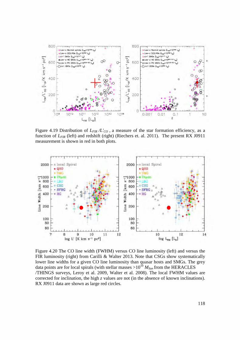
118

Figure 4.19 Distribution of LFIR /L'CO , a measure of the star formation efficiency, as a function of LFIR (left) and redshift (right) (Riechers et. al. 2011). The present RX J0911 measurement is shown in red in both plots.

Figure 4.20 The CO line width (FWHM) versus CO line luminosity (left) and versus the FIR luminosity (right) from Carilli & Walter 2013. Note that CSGs show systematically lower line widths for a given CO line luminosity than quasar hosts and SMGs. The grey data points are for local spirals (with stellar masses >1010 MSun from the HERACLES /THINGS surveys, Leroy et al. 2009, Walter et al. 2008). The local FWHM values are corrected for inclination, the high z values are not (in the absence of known inclinations). RX J0911 data are shown as large red circles.

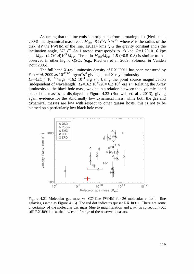
119

Assuming that the line emission originates from a rotating disk (Neri et. al. 2003) the dynamical mass reads Mdyn=R∆V2G–1sin–2i where R is the radius of the disk, ∆V the FWHM of the line, 120±14 kms–1, G the gravity constant and i the inclination angle, 67o±8o. As 1 arcsec corresponds to ~8 kpc, R=1.20±0.16 kpc and Mdyn=(4.7±1.4)109 MSun. The ratio Mdyn/Mgas=1.5 (+0.5–0.8) is similar to that observed in other high-z QSOs (e.g., Riechers et al. 2009; Solomon & Vanden Bout 2005).

The full band X-ray luminosity density of RX J0911 has been measured by Fan et al. 2009 as 10-12.62 ergcm-2s-1 giving a total X-ray luminosity LX=4πDL

2 10-12.62ergs-1=162 1044 erg s-1. Using the point source magnification (independent of wavelength), LX=162 1044/26= 6.2 1044 erg s-1. Relating the X-ray luminosity to the black hole mass, we obtain a relation between the dynamical and black hole masses as displayed in Figure 4.22 (Bothwell et. al . 2013), giving again evidence for the abnormally low dynamical mass: while both the gas and dynamical masses are low with respect to other quasar hosts, this is not to be blamed on a particularly low black hole mass.

Figure 4.21 Molecular gas mass vs. CO line FWHM for 36 molecular emission line galaxies, (same as Figure 4.16). The red dot indicates quasar RX J0911. There are some uncertainty of the molecular gas mass (due to magnification and L'CO(1-0) correction) but still RX J0911 is at the low end of range of the observed quasars.

120

Figure 4.22 MBH-σ relation for SMGs (blue circles) in the Bothwell 2013 sample. Black hole masses were obtained from measured X-ray luminosities following Alexander et al. 2005. The same quantities for local elliptical galaxies, as presented by Gultekin et al. 2009, with the best-fit (slope β=4.24) are shown as black triangles and red-dot curve.

121

5. Summary and perspectives The study presented here has given a detailed account of observations of

the host galaxy of a distant quasar, RX J0911, using millimetre wavelengths. It has been used as a case study to illustrate and comment on major features displayed by galaxies in the early Universe. Information obtained about the properties of such galaxies (here z=2.8) contribute to a better understanding of the formation and evolution of structures at the epoch of galaxy assembly during which most stars have been formed. Detailed observations of CO emission have been made possible thanks to the gravitational lensing offered by the presence of a galaxy in the foreground and to the quality of the Plateau de Bure Interferometer. High resolutions have been obtained both in frequency, allowing for a precise measurement of the line width, and in space, allowing for resolving spatially the source both on the line and in the continuum, namely both in its dust and gas content.

The mechanism of gravitational lensing has been discussed in very precise details. As is often the case with lensing events resulting in large magnifications – here typically in the ×15 to ×35 range – the source happens to be in the vicinity of the lens caustic, in fact to overlap it. A consequence of this particularity is a strong dependence of the magnification on the precise position of point sources in the galaxy, resulting in significantly different magnifications for the gas, the dust and the central QSO. Moreover, the morphology of the observed images is distorted in addition to being amplified. The contribution of the present work in this domain has been essential, many of the related subtleties being often overlooked in the literature: it can serve as a guide for future observations of this and similar lensed galaxies. The data that have been obtained illustrate well the invaluable advantage offered by strong lensing in terms of increased sensitivity as well as the complication that results, causing an additional source of uncertainties on the quantities that are accessible to measurement. Two different lensing potentials have been used, offering complementary advantages and weaknesses, and the comparison between their predictions has provided a deeper understanding of the lensing mechanism than would have been possible otherwise.

The CO(7-6) line stands out clearly above continuum, allowing for reliable measurements of the gas and dust luminosities. Detailed studies of the four lensed images have made it possible to resolve the source in both the line and the continuum with rms radii of 106±15 and 39±18 mas respectively, corresponding to 0.85±0.12 kpc and 0.31±0.14 kpc respectively. In the line case, the quality of the data have further provided evidence for an ellipticity of the source, with an ellipticity parameter (square root of the ratio between major and minor axes) of 1.60 (+0.35−0.18) and a position angle (of the major axis) of 111o±9o, 3.3 standard deviations away from a circular source hypothesis. Moreover, evidence for a

122

velocity gradient correlated with the source ellipticity has been obtained at the level of 4.5 standard deviations.

A remarkable feature of the CO(7-6) line is its very small width, typically a factor 2 to 3 lower than for similar quasar hosts. As a result, the dynamical mass is very low. Indeed, both gas and dust mass evaluations also fall on the low side of the normal high-z quasar host population. The large star formation efficiency places RX J0911 on the high side of both low-z and high-z galaxies, suggesting that it is in a state where much of its gas has been exhausted after an intense star formation period, leaving it at the border between high-z and low-z quasar hosts. This pleads against an interpretation of the small line width being the result of the disk being seen face-on and adds to the argument of a significant source ellipticity to suggest that RX J0911 is indeed at the border between high-z and low-z quasar hosts.

The recent availability of ALMA, with greatly increased sensitivity and improved resolution with respect to Plateau de Bure, invites an extension of the present study. In a first stage, we have selected for this a quasar host similar to RX J0911 but with an even larger magnification, in excess of 100, B1359+154. The material reviewed in order to reach this choice is summarized in Appendix A3. It has a redshift z=3.24 and is both radio loud and optically bright. As RX J0911, it overlaps the lens caustic and has the particularity of being lensed by three lens galaxies, resulting in six images that ALMA could resolve in three separate blobs. As described in Appendix A4, an unprecedented resolution of ~50 pc in the source plane could be reached with only 2 hours of observation. In addition to the CO(9-8) line, the water line could also be observed, giving useful information on the FIR luminosity.

The observation of quasar hosts at high redshifts has a rich future in front of it that will undoubtedly contribute to improving our understanding of the formation and evolution of structures in the early Universe. We hope to have opportunities to use the experience acquired with the study of RX J0911 in taking an active part in such explorations.

123

References Credit: the general presentations of the topics dealt with in the thesis have their sources where I learned about them: Lectures by my supervisors, Dr Frederic Boone and Pr Pierre Darriulat, lectures by Pr Françoise Combes in Ha Noi (2013), lectures at the IRAM schools at Granada (2011) and Grenoble (2012), various standard text books and Wikipedia articles, in particular on quasars and galaxies. In addition review articles such as Carilli & Walter (2013) and Elbaz et al. (2011) have been very rich sources of information. While having never copied any statement from such sources without having made sure that I understand it in depth, I did not attempt to rephrase artificially statements that were saying what they had to say in the best possible way.

Abel T., M. L. Norman and P. Madau, ApJ 523 (1999) 66. Alexander D. M., et al. 2005 Ap. J. 632:736–50. Anh, P. T. et al., 2012, A&A, 552, 2013. Alton P. B., J. Lequeux, S. Bianchi, D. Churches, J. Davies and F. Combes, A&A 366 (2001) 451. Bechtold J., et al. 2001, Astrophys. J. 562, 133. Bade, N. et al., A&AS 110 (1995) 469. Bade, N. et al., A&AS 317 (1997) L13. Barnes, J. E. 1988, ApJ, 331, 699. Barnes, J. E. & Hernquist, L. 1992, ARA&A, 30, 705. Bartelmann, M., 2003, Numerical Methods in Gravitational Lensing, Proc.

Gravitational Lensing Winter School, Aussois. Barvainis R. and Ivison R. (2002) The Astrophys. J., 571, 712-720. Beaulieu et al., 2006, Nature, 439, 437. Beelen, A., et al. 2006, ApJ, 642, 694. Belokurov et al., 2007, ApJ, 671L, 9. Benford D. J., P. Cox, A. Omont, T. G. Phillips and R. G. McMahon,

ApJ 518 (1999) L65. Blain, A. W., MNRAS, 304 (1999a) 669. Blain A. W. , D. T. Frayer, J. J. Bock and N. Z. Scoville, MNRAS 313 (2000) 559. Blain, A. W., Smail, I., Ivison, R. J., Kneib, J., & Frayer, D. T.

2002, Phys. Rep., 369, 111. Blain, A.W., Barnard, V.E., & Chapman, S.C. 2003, MNRAS, 338, 733. Blandford, R.D. & Kochanek, C.S. 1987, ApJ, 321, 658. Blandford, R.D. et al. 1989, Science, 245, 824. Bolatto A. D., Wolfire M., Leroy A. K., 2013, ARA&A, 51, 207 Boller et al., 1997, MNRAS, 289, 393. Bolton et al., 2006, ApJ, 646L, 45. Bond et al., 2004, ApJ, 606L, 155. Boone, F., Schaerer, D., Pelló, R., Combes, F., & Egami, E. 2007, A&A,

124

475, 513. Bothwell M, Chapman SC, Tacconi L, Smail I, Ivison RJ, et al. 2010. MNRAS 405:219–33. Bothwell, M. S., Smail, I., Chapman, S. C., et al. 2013, MNRAS, 429,

3047. Bouwens, R. J., et al. 2011, Nature, 469, 504. Burud, I. et al. 1998, ApJ, 501, L5. Burud, I., et al. 2002b, A&A, 391, 481. Cabanac et al., 2005, A&A, 436L, 21. Calzetti, L. Armus, R. C. Bohlin, A. L. Kinney, J. Koornneef and

T. Storchi-Bergmann, ApJ 533 (2000) 682. Carilli, C. L. & Barthel, P. D. 1996, A&A Rev., 7, 1. Carilli CL, Cox P, Bertoldi F, Menten KM, Omont A, et al. 2002a. Ap. J.

575:145–9. Carilli CL, Blain AW. 2002b. Ap. J. 569:605–10. Carilli C. L., Walter F., 2013, ARA&A, 51, 105. Castro-Carrizo A., Neri R., Sept. 2010., IRAM Plateau de Bure Interferometer Data Reduction Cookbook, IRAM. Chapman, S. C., Blain, A. W., Smail, I., Ivison, R. J. 2005, ApJ, 622, 772. Clavel et al., 1991, ApJ, 366, 64C. Daddi, E., Dickinson, M., Morrison, G. et al. 2007a, ApJ, 670, 156. Dekel A, Sari R, Ceverino D. 2009a. Ap. J. 703:785–801. Dekel A, Birnboim Y, Engel G, Freundlich J, Goerdt T, et al. 2009b. Ap. J. 457:451–4. Do Thi Hoai et al., 2013, Res. Astron. Astrophys. Vol 13, No 7. Domingue D. L., W. C. Keel, S. D. Ryder and R. E. White, AJ 118 (1999) 1542. Dominik, M., 1988, A&A, arXiv:astro-ph/9804.59v1 6 Apr and references therein. Dong et al., 2009, ApJ, 698, 1826. Draine B. T. and Lee H. M., ApJ 285 (1984) 89. Draine B. T. and Li A., ApJ 551 (2001) 807. Devriendt J. E. G., B. Guiderdoni and R. Sadat, A&A 350 (1999) 381. Downes, D. & Solomon, P. M. 1998, ApJ, 507, 615. Dunne, L., Eales, S., Edmunds, M., Ivison, R., Alexander, P.,

& Clements, D.L. 2000, MNRAS, 315, 115. Dunne, L., & Eales, S. A. 2001, MNRAS, 327, 697. Elbaz, D., Dickinson, M., Hwang, H. S., et al. 2011, A&A, 533, A119. Elíasdóttir, Á., et al., 2007, ArXiv e-prints, arXiv:0710.5636. Elmegreen BG, Burkert A. 2010. Ap. J. 712:294–302.

Faber, S. M. & Jackson, R. E., 1976, Astrophys. J., 204, 668. Falco et al., 1996, AJ, 112, 897F.

Fan, L. L., Wang, H. Y., Wang, T., et al. 2009, ApJ, 690, 1006

125

Ferrarese, L. & Merritt, D.,2000, ApJ, 539, L9. Flower DR, & Launay JM 1985. MNRAS 214:271. Fort, B. & Mellier, Y., 1994, A&ARv, 5, 239F. Frayer DT, Ivison RJ, Scoville NZ, Yun M, Evans AS, et al. 1998. Ap. J. Lett. 506:L7–L10. Fukugita M, Peebles PJE. 2004. Ap. J. 616:643–68. Geach JE, Smail I, Moran SM, MacArthur LA, Lagos CDP, Edge AC. 2011. Ap. J. 730:L19. Gilmore, G., & Reid, I. N. 1983, MNRAS, 202, 1025. Gilmore, G., Wyse, R. F. G., & Kuijken, K. 1989, ARA&A, 27, 555. Granato G. L., L. Danese and A. Franceschini, ApJ 460 (1996) L11. Greenstein & Schmidt, 1964, ApJ, 140, 1G. Grenoble Imaging and Line Data Analysis System (GILDAS), 2008, IRAM. http://www.iram.fr/IRAMFR/GILDAS. Gültekin, K., Richstone, D. O., Gebhardt, K., et al. 2009, ApJ, 698, 198. Guiderdoni B. ,Hivon E. , F. R. Bouchet and B. Maffei, MNRAS 295 (1998) 877. Hainline, L.J., et al., ApJ 609 (2004) 61. Hagen, H.-J. et al., A&AS 111 (1995) 195. Hogbom, J. A. 1974, A&A suppl., 15, 417. Holt et al. 1992, Testing the AGN Paradigm (New York: AIP). Hopkins PF, Hernquist L, Cox TJ, Di Matteo T, Robertson B, Springel V. 2006. Ap. J. Suppl. 163:1–49. Hjorth, J., et al., 2002, ApJ, 572, L11. Hildebrand R. H., QJRAS 24 (1983) 267. Hodge JA, Carilli CL, Walter F, de Blok WJG, Riechers D, et al. 2012.

Ap. J. 760, 11. Hu W., 2000, Phys. Rev. D, 62, 043007. Hughes D., in Bremer M. N., van der Werf P. P., Rottgering H. J. A. and

Carilli C. L. eds., Cold Gas at High Redshift, Kluwer (1996) p. 311. Ishida, C. M. 2004, PhD thesis, AA(UNIVERSITY OF HAWAII). Ivison R. J., I. Smail, A. J. Barger, J.-P. Kneib, A. W. Blain, F. N. Owen, Kerr T. H. and L. L. Cowie, MNRAS 315 (2000a) 209. Ivison R. J., I. Smail, D. T. Frayer, J.-P. Kneib and A. W. Blain,

ApJ 561(2001), L45. Ivison RJ, Papadopoulos PP, Smail I, Greve TR, Thomson A, et al. 2011. MNRAS 412:1913–25. Isaak K. G. et al., MNRAS 329 (2002) 149. Jullo, E. & al., 2007, New J. Phys. 9, 447 and references therein. Jullo, E. and Kneib. J.-P., 2009, arXiv:0901.3792v3 [astro-ph.CO]

21 Feb 2009. Kartaltepe, J. S. & Balonek, T. J. 2007, AJ, 133, 2866. Kassiola, A. & Kovner, I. 1993, ApJ, 417, 450.

126

Kennicutt, R. C., Jr. 1998b, ApJ, 498, 541. Keres D., Katz N., Weinberg D., Dave R. 2005. MNRAS 363:2–28. Keres D., Katz N., Fardal M., Dave R., Weinberg D.H. 2009. Ap. J. 395:

160–79. Kirk, J. M., et al. 2010, A&A, 518, L82. Kneib, 1993, PhD Thesis, Univ. Paul Sabatier, Toulouse. Kneib et al., 1995, A&A, 303, 27. Kneib, J.-P., Cohen, J.G. and Hjorth, J. 2000, ApJ, 544, L35. Kneib, J.-P., and Jullo, E., 2009, Mon. Not. R. Astron. Soc., 395/3 1319;

see also http://www.oamp.fr/cosmology/lenstool and M. McCourt, An Undergraduate’s First Encounter with Lenstool, October22 2006, www.oamp.fr/cosmology/lenstool/lenstool_dummies.pdf.

Kneib, J.-P., 2012, Cluster strong lensing as a probe of the high redshift universe, Lectures given at the XIth School on Cosmology, Cargèse, 17-22 September 2012 and references therein. Kochanek, C.S. et al., CfA-Arizona Space Telescope LEns Survey

(CASTLES), http://www.cfa.harvard.edu/castles/ Kochanek, C.S., 2002, Gravtational Lenses, the Distance Ladder and

the Hubble Constant: a New Dark Matter Problem, arXiv:astro-ph 0204043v1 2002.

Kochanek, C.S. et al., 1999, in American Institute of Physics Conference Series, Vol.470, ed. S. Holt & E. Smith, 163-175 7. Kochanek, C. S. 2006, in Saas-Fee Advanced Course 33: Gravitational Lensing: Strong, Weak and Micro, ed. G. Meylan, P. Jetzer, P. North, P. Schneider, C. S. Kochanek, & J. Wambsganss, 91–268 Kormendy J., Ho L. C., 2013, ARA&A, 51, 511. Leroy AK, Walter F, Brinks E, Bigiel F, de Blok WJG, et al. 2008,

Astron. J. 136:2782–845. Lucas R. and Gueth F., Continuum and Line Interferometer Calibration (CLIC), IRAM. Lynds, R. & Petrosian, V., 1989, ApJ, 336, L1. Magnelli, B., Elbaz, D., Chary, R.R., et al. 2009, A&A, 496, 57. Magnelli, B., Elbaz, D., Chary, R.R., et al. 2011, A&A, 528, 35. Maiolino R, Gallerani S, Neri R, Cicone C, Ferrara A, et al. 2012. MNRAS

425:L66–L70. Marchesini, D., van Dokkum, P.G., Forster Schreiber, N. M., et al. 2009, ApJ, 701, 1765. Martig M., Bournaud F., Teyssier R., Dekel A., 2009, ApJ, 707, 250. Morgan, N.D. et al., 2001, ApJ, 555, 1. Moster BP, Somerville RS, Maulbetsch C, van den Bosch FC, Maccio AV, et al. 2010. Ap. J. 710:903–23. Mullaney et al., 2012, MNRAS, 419, 95. Munshi D., Valageas, P., Van Waerbeke, L., Heavens, A., 2008, Physics

127

Reports, 462, 67. Murphy, T.W.,Jr., Armus, L., Matthews, K. et al. 1996, AJ, 111, 1025. Naab, T., & Burkert, A. 2003, ApJ, 597, 893. Negroponte, J. & White, S. D. M. 1983, MNRAS, 205, 1009. Neri R., et al., 2003, ApJ, 597, L113. Omont A., P. Cox, F. Bertoldi, R. G. McMahon, C. Carilli and K. G. Isaak, A&A 374 (2001) 371. Paczynski, B. 1986, ApJ, 304, 1. Paris, I., Petitjean, P., Aubourg, E., et al. 2012, A&A, 548, A66. Paris, I., Petitjean, P., Aubourg, E., et al. 2014, A&A, 563A, 54. Pety J., 2007, MAPPING a GILDAS software, IRAM. Peeples, M.S., 2003,

http://www.astronomy.ohio-state.edu/~molly/lenses/RX J0911 ,html. Preston, G.W., Beers, T. C., & Shectman, S. A. 1994, AJ, 108, 538. Priddey R. S. and McMahon R. G., MNRAS 324 (2001) L17. Richard, J.; Kneib, J.-P.; Limousin, M. ; Edge, A.; Jullo, E., 2010, MNRAS, 402L, 44. Riechers DA, Walter F, Brewer BJ, Carilli CL, Lewis GF, et al. 2008a.

Ap.J. 686:851–8. Riechers DA, Walter F, Carilli CL, Bertoldi F, Momjian E. 2008b.

Ap. J. 686:L9–L12. Riechers, D. A., Walter, F., Carilli, C. L., & Lewis, G. F. 2009,

ApJ, 690, 463. Riechers DA, Walter F, Carilli CL, Lewis GF. 2009b. Ap. J. 690:463–85 Riechers, D. A. 2011, ApJ, 730, 108. Riechers DA, Carilli CL, Maddalena RJ, Hodge J, Harris AI, et al. 2011a.

Ap. J. Lett. 739:L32. Rosario et al., 2012, A&A, 545, A45. Saha, P. & Williams, L.L.R. 2003, AJ, 125, 2769. Sanders, D.B., Soifer, B.T., Elias, J. H. et al. 1988, ApJ, 325, 74. Sakamoto K., N. Z. Scoville, M. S. Yun, M. Crosas, R. Genzel and

L. Tacconi, ApJ 514 (1999) 68. Schechter, P.L., Proceedings IAU Symposium No. 225, 2004, in press

arXiv:astro-ph0408338v1. Schechter, P.L. 2005 in IAU Symposium, Vol. 225, Gravitational Lensing Impact on Cosmology, ed. Y. Mellier & G. Meylan, 281 Schmidt, M. 1963, Nature, 197, 1040. Schneider, D. P., Richards, G. T., Hall, P. B., et al. 2010, AJ, 139, 2360. Shin et al., 2012, ApJ, 760, 116. Seljak, U.; Zaldarriaga, M.; 1999, Physical Review Letters, 82, 2636. Solomon PM, Downes D, Radford SJE. 1992a. Astrophys. J. 398:L29–32. Solomon PM, Vanden Bout PA. 2005. ARA&A 43:677–725. Soucail, G., et al., 1987, A&A, 172, L14.

128

Springel et al., 2005, Nature 435, 629. Suyu, S.H. & Blandford, R.D., 2005, The anatomy of a quadruply imaged gravitationally lensed system, SLAC-PUB-11293, 2005, Revised. Suyu, S.H. et al., 2009, arXiv:astro-ph/08042827v3 [astro-ph] 12 Jan 2009. Steven Weinberg, Gravitation and cosmology principles,

John Wiley & Sons, Inc. 1972. Tully, R. B. & Fisher, J. R., 1977, Astron. Astrophys., 54, 661.

Veilleux, S., Kim, D.-C., Sanders, D. B. 2002, ApJS, 143, 315. Venturini, S. & Solomon, P. M., 2003, ApJ, 590, 740V. Walker, I. R., Mihos, J. C. & Hernquist, L. 1996, ApJ, 460, 121. Walsh, Carswell & Weymann, 1979, Nature, 279, 381. Walter F, Carilli C, Bertoldi F, Menten K, Cox P, et al. 2004.

Ap. J. 615:L17–L20. Walter F, Brinks E, de Blok WJG, Bigiel F, Kennicutt RC, et al., 2008,

Astron. J. 136:2563. Wambsganss J., "Gravitational Lensing in Astronomy", Living Rev.

Relativity 1, (1998), 12, http://www.livingreviews.org/lrr-1998-12 Wilson C. D. , Scoville N., Madden S. C. and Charmandaris V. ,

ApJ 542 (2000) 120. Weiss, A., Walter, F., Downes, D., et al. 2012, ApJ, 753, 102 Witt, H.J. and Mao, S. MNRAS 291 (1997) 211. Wu, J., Vanden Bout, P. A., Evans, II, N. J., & Dunham, M. M. 2009,

ApJ, 707, 988. Yang B, Stancil PC, Balakrishnan N, Forrey RC. 2010. Ap. J. 718:1062. York, D. G., Adelman, J., Anderson, Jr., J. E., et al. 2000, AJ, 120, 1579. Young, L. M. et al., 2011. MNRAS 414, 940. Zwicky, F., 1937, Phys. Rev. Lett., 51, 290.

129

Appendices

A1. Line emission

At high redshift, there are two commonly used ways to express line luminosity (Carilli & Walter 2013). From energy conservation, vrest L(vrest)=4πD2

Lvobs S(vobs), where L is the luminosity (J), S the observed flux density in W/Hz, DL the luminosity distance. Using standard relations from S. Weinberg (1972), S(vobs)=P(vobsR(t0)/R(t1))R(t1)/R

3(t0)r12 where P is the intrinsic power, the power

emitted per unit solid angle and per unit frequency interval (W/Hz/sr). From the definition of redshift, z = R(t0)/R(t1)−1 vrest = vobs R(t0)/R(t1) = vobs (1+z). One can rewrite: S(vobs) = P(vres)R(t1)/R

3(t0)r12 = P(vres)/(1+z)R2(t0)

r12

From the relation between R(t1)r1 is and the angular distance described by DA=R(t1)r1 we find S(vobs)=P(vres)/(1+z)3DA

2 Using DA=DL/(1+z)2 one can rewrite: S(vobs)=P(vres)(1+z)/DL

2 P is power per unit solid angle per unit frequency interval, so: P=L/4π

where L is the power emitted per unit frequency interval (W/Hz), so: S(vobs)=L(vres)(1+z)/4π DL

2 which is equivalent to vrest L(vrest)=4πD2Lvobs S(vobs)

(Solomon et. al. 2005) The total luminosity over the line (W) is L'= ∫L(vres)dvres ~ L(vres)∆vres and S(vobs) = L'(1+z)/4π ∆vresDL

2 Note that ∆vres = vres ∆Vres/c so L' = 4π S(vobs)vres ∆VresDL

2/c(1+z) Using the same units as Solomon et. al. (2005), namely L' in solar

luminosity, S in Jy, velocity in km/s, frequency in GHz, and luminosity distance in Mpc: L''=L'/L Sun=L'/3.839.1026, S'=S*1026, ∆V'=∆Vres/103, v'=vrest/109, DL'=D L/3.09 1022. Then: L'' = 1.04 10−3 S' ∆V' v' DL

2'/(1+z) = 1.04 10−3 S' ∆V' vobs DL2'

From here, one can express the source luminosity in LSun: Lline=1.04 10–3 Sline∆V D2

L vobs LSun With Sline∆V in Jy km s–1 ; vobs in GHz; D2

L in Mpc; Lline is expressed as the source luminosity in LSun or other rational units. L'line

is expressed via the (area) integrated source brightness temperature, in units of K km s–1pc2. The line luminosity is expressed as the product of the velocity integrated source brightness temperature (see Solomon et. al. 1992), Tb∆V and the source area, ΩSDA

2, where ΩS is the solid angle subtended by the source and the angular size distance DA. The observed integrated line intensity, ICO= ∫Tbdv measures the beam diluted brightness temperature, which also decreases with redshift, Tb∆VΩs=I CO Ωs*b(1+z), where Ωs*b is the solid angle of the source

130

convolved with the telescope beam. Therefore, the line luminosity L'CO=Tb∆VΩsDA

2= Ωs*b DL2ICO (1+z)–3

with Ω's*b = (π 180–13600–1)Ωs*b in arcsec2 ; D'L=106DL in pc2 L'CO=23.5 Ω's*b D'L

2ICO (1+z)–3 where L'CO is in K km s–1pc2 The line luminosity, L'CO can also be expressed for a source of any size in

terms of the total line flux, using Rayleigh-Jean approximation, Tb=(c2/2k)Iv/v2:

L'line=(c2/2k) Sline ∆V vobs–2 D2

L (1+z)–3 where c = 3.108 m/s; k=1.3810–23 JK–1 D'L=106 DL in pc2; S'line=Sline10–26J; v'=109v

L'line = 3.25 107 Sline ∆v D2L(1+z)–3vobs

–2 K km s–1pc2 where Sline ∆v is in Jy km s–1; DL in Mpc; vobs in GHz; L' line in K km s–1pc2 Both Lline and L′line have their justification: e.g. if one is interested in

comparing the power that is being emitted through a given line to calculate the cooling capability (e.g. in relation to the FIR luminosity, Lline /LFIR ) one uses the Lline definition. The L'line is commonly used to translate measured CO luminosities to H2 masses using the conversion factor α. Also, for thermalized molecular gas emission L′line is approximately constant for all transitions.

Reference

Carilli C. L., Walter F., 2013, ARA&A, 51, 105. Steven Weinberg, Gravitation and cosmology: principles and applications of the general theory of relativity, Wiley, Aug 11, 1972. Solomon, P. M.; Downes, D.; Radford, S. J. E., 1992, Ạp, 398L, 29. Solomon PM, Vanden Bout PA. 2005. ARA&A 43:677–725.

131

A2. Dust emission

The material in this part is mainly taken from the paper of Blain A. W. et al. 2002 about submm galaxies.

The dust emission process is thermal, with dust grains emitting a modified blackbody spectrum. Grains of interstellar dust, distributed throughout the ISM of a galaxy, are heated to temperatures between about 20 and 200 K, depending on the spectrum and intensity of the interstellar radiation field (ISRF), and the size and optical properties of the grains. Higher dust temperatures can be produced close to a powerful source of radiation, with dust subliming at temperatures of order 2000 K. Very small grains can be heated far above their equilibrium temperatures by absorbing hard UV photons (see Draine and Li, 2001). Lower dust temperatures, always exceeding the CMB temperature in the z<3 range, are possible in opaque regions of the ISM that are shielded from intense heating, in the intergalactic medium or in regions with an intrinsically weak ISRF. Unless dust is heated by the ISRF in addition to the CMB the galaxy will not be detectable.

We now consider the properties of the dust emission that are relevant to observations of high redshift galaxies. The minimum set of parameters necessary to describe the emission from dust grains are a temperature Td and a form of the emissivity function, εν. The distribution of dust temperatures reflects the different nature and environment of each grain in the galaxy. It is useful to use Td to describe the coolest grains that contribute significantly to the energy output of a galaxy when discussing submillimeter observations. In most cases, spatially and spectrally resolved images of galaxies are not available, and so it is reasonable to assume a volume averaged description of the emissivity function as a function of frequency ν, εν~ν

β. Values of β in the range of 1 to 2 are usually assumed. Scattering theory predicts that β→2 at low frequencies, while a value β=1 at high frequencies matches the general trend of the interstellar extinction curve that describes the properties of absorption of optical and UV radiation by the ISM (see Calzetti et al., 2000).

The simplest form of the SED emission spectrum is fν~ενBν, where Bν is the Planck function (2kTdν

2/c2 in the Rayleigh-Jeans limit, in units of Wm−2Hz−1sr−1). This assumes that the emitting source is optically thin. When fitting SMG spectra, one assumes such a simple SED functional form whether at large z or at low z as Dunne et al. (2000) and Dunne and Eales (2001) do. However, it is useful, at small wavelengths, to account for optical depth by using a form fν~[1−exp(−τν )]Bν, where τν is the frequency-dependent optical depth of the cloud, and is a multiple of εν. This form tends to the simpler ενBν form at long wavelengths, and is used by Benford et al. (1999), Omont et al. (2001), Priddey and McMahon (2001) and Isaak et al. (2002), on submillimeter data of high-redshift AGNs (with rest-frame frequencies that are relatively close to the peak of the SED). The extra parameter

132

required to relate τν and εν can be defined as the frequency at which τν=1 where the cloud becomes optically thick. If the opacity near a wavelength of 100 µm is large, then the form of the peak of the SED tends to that of a blackbody spectrum. This suppresses emission near the SED peak relative to the emission in the Rayleigh–Jeans regime, and so this functional form provides a good fit to a set of submillimeter and FIR data with a higher value of Td than compared with the ενBν form, by typically ~10–20%. However, as most observed SEDs of high-redshift galaxies use less than four data points (see Fig. 4.17), the use of four parameters is unlikely to be meaningful.

Figure A2.1 describes various observed rest frame spectral energy distributions (SEDs) of galaxies from the radio to the near-IR wavebands. Three template SEDs are shown. One includes the properties of CO and atomic fine-structure emission lines in the (sub)millimeter waveband (100 to 3000 µm, Blain et al., 2000b), one includes polycyclic aromatic hydrocarbon (PAH) molecular emission features at ~10 microns in the mid-IR waveband (Guiderdoni et al. 1998), and one is normalized to the typical SED of a sample of low-redshift IRAS galaxies (Dunne et al., 2000).

It is reasonable to assume that the mid-IR SED can be smoothly interpolated from a modified blackbody function at low frequencies to a power-law fν~ν

α in the mid-IR waveband on the high-frequency side of the spectral peak, in order to prevent the high-frequency SED from falling exponentially with a Wien spectrum. Hotter components of dust, emitting at shorter wavelengths, and ultimately stellar emission in the near-IR waveband, are certain to be present to reduce the steepness of the SED in the Wien regime. That an exponential Wien spectrum is inappropriate can be seen from the well-defined power-law mid-IR SEDs of Arp 220 and Mrk 231 shown in Figure A2.1.

Figure A2.1 Various observed rest frame spectral energy distributions (SEDs) of galaxies from the radio to the near-IR wavebands (see text).

133

Given the current lack of resolved images of distant galaxies in the submm and FIR wavebands, it is important to neither over-parameterize the descriptions nor overinterpret the results of observations of their SEDs. When spatially resolved, high-spectral resolution images are available, building on existing interferometric images of low-redshift dusty galaxies (Downes and Solomon, 1998; Sakamoto et al., 1999; Wilson et al., 2000), it should be possible to study the radiative transfer from sites of intense star formation and AGN in these geometrically complex opaque galaxies (see Ivison et al., 2000a, 2001). Models of the SEDs of dust-enshrouded AGN at different viewing angles have been developed by Granato et al. (1996), while star-forming regions embedded in a disk geometry have been analyzed by Devriendt et al. (1999). More powerful and efficient radiative-transfer codes have been developed (for example Abel et al., 1999), and it should be practical to develop detailed models of the appearance of galaxies with realistic geometries to account for future, high resolution multi-band submm images.

It is conventional to introduce a frequency-dependent mass-absorption coefficient κν [m

2/kg] (Draine and Lee, 1984), proportional to εν, as the ‘effective area’ for black body emission by a certain mass of dust,

L/4π = Md κν(vrest)Bv(vrest ,Td) or Md = S(vobs)D

2L/(1+z)κν(vrest)Bv(vrest ,Td)

where Bv is the Planck function. Values of κν at a conventional frequency of ~1 mm are in the range of 0.04 to 0.15 m2kg−1 (Hughes, 1996). Recent comparisons of optical extinction and submillimeter emission from partially resolved edge-on spiral galaxies have tended to give values of 0.05 to 0.4 m2 kg−1 (Alton et al., 2001). Domingue et al. (1999) derive 0.09 m2 kg−1 from similar FIR, optical and submm data. Dunne et al. (2000) adopt a value of 0.077 m2 kg−1 . Note that there is at least a factor of 3 uncertainty in these conversion factors.

An alternative dimensionless function Qν (Hildebrand, 1983) is sometimes used, which includes information about the mass/volume and surface area of a typical grain. If grains are assumed to be spherical (a big if), with bulk density ρ, radius a, and an emissive cross section πa2, then κν=3Qν/4aρ. Qν Bν is the effective emissivity function describing the energy flux from unit area of the dust grain surface. However, dust grains are more likely to be irregular in shape, possibly colloidal or in the form of whiskers. In that case, the emissivity per unit mass would be increased, and the dust mass associated with a fixed luminosity would be overestimated.

References Abel T., M. L. Norman and P. Madau, ApJ 523 (1999) 66. Alton P. B., J. Lequeux, S. Bianchi, D. Churches, J. Davies and F. Combes,

A&A 366 (2001) 451. Benford D. J., P. Cox, A. Omont, T. G. Phillips and R. G. McMahon,

ApJ 518 (1999) L65.

134

Blain A. W. , D. T. Frayer, J. J. Bock and N. Z. Scoville, MNRAS 313 (2000) 559.

Blain, A. W., Smail, I., Ivison, R. J., Kneib, J., & Frayer, D. T. 2002, Phys. Rep., 369, 111

Calzetti, L. Armus, R. C. Bohlin, A. L. Kinney, J. Koornneef and T. Storchi-Bergmann, ApJ 533 (2000) 682.

Devriendt J. E. G., B. Guiderdoni and R. Sadat, A&A 350 (1999) 381. Domingue D. L., W. C. Keel, S. D. Ryder and R. E. White, AJ 118 (1999)

1542. Downes, D. & Solomon, P. M. 1998, ApJ, 507, 615. Draine B. T. and Lee H. M., ApJ 285 (1984) 89. Draine B. T. and Li A., ApJ 551 (2001) 807. Dunne, L., Eales, S., Edmunds, M., Ivison, R., Alexander, P.,

& Clements, D.L. 2000, MNRAS, 315, 115 Dunne, L., & Eales, S. A. 2001, MNRAS, 327, 697 Granato G. L., L. Danese and A. Franceschini, ApJ 460 (1996) L11. Guiderdoni B. ,Hivon E. , F. R. Bouchet and B. Maffei, MNRAS 295

(1998) 877. Hildebrand R. H., QJRAS 24 (1983) 267. Hughes D., in Bremer M. N., van der Werf P. P., Rottgering H. J. A. and

Carilli C. L. eds., Cold Gas at High Redshift, Kluwer (1996) p. 311. Isaak K. G. et al., MNRAS 329 (2002) 149. Ivison R. J., I. Smail, A. J. Barger, J.-P. Kneib, A. W. Blain, F. N. Owen,

Kerr T. H. and L. L. Cowie, MNRAS 315 (2000a) 209. Ivison R. J., I. Smail, D. T. Frayer, J.-P. Kneib and A. W. Blain,

ApJ 561(2001), L45. Omont A., P. Cox, F. Bertoldi, R. G. McMahon, C. Carilli and K. G. Isaak, A&A 374 (2001) 371 Priddey R. S. and McMahon R. G., MNRAS 324 (2001) L17. Sakamoto K., N. Z. Scoville, M. S. Yun, M. Crosas, R. Genzel and

L. Tacconi, ApJ 514 (1999) 68. Wilson C. D. , Scoville N., Madden S. C. and Charmandaris V. ,

ApJ 542 (2000) 120.

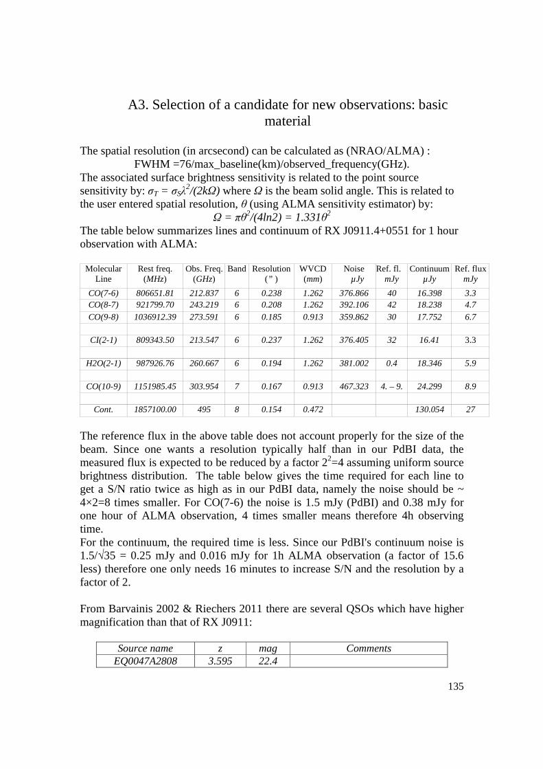
135

A3. Selection of a candidate for new observations: basic material

The spatial resolution (in arcsecond) can be calculated as (NRAO/ALMA) :

FWHM =76/max_baseline(km)/observed_frequency(GHz). The associated surface brightness sensitivity is related to the point source sensitivity by: σT = σSλ

2/(2kΩ) where Ω is the beam solid angle. This is related to the user entered spatial resolution, θ (using ALMA sensitivity estimator) by:

Ω = πθ2/(4ln2) = 1.331θ2 The table below summarizes lines and continuum of RX J0911.4+0551 for 1 hour observation with ALMA:

Molecular Line

Rest freq. (MHz)

Obs. Freq. (GHz)

Band Resolution (” )

WVCD (mm)

Noise µJy

Ref. fl. mJy

Continuum µJy

Ref. flux mJy

CO(7-6) 806651.81 212.837 6 0.238 1.262 376.866 40 16.398 3.3 CO(8-7) 921799.70 243.219 6 0.208 1.262 392.106 42 18.238 4.7

CO(9-8) 1036912.39 273.591 6 0.185 0.913 359.862 30 17.752 6.7

CI(2-1) 809343.50 213.547 6 0.237 1.262 376.405 32 16.41 3.3

H2O(2-1) 987926.76 260.667 6 0.194 1.262 381.002 0.4 18.346 5.9

CO(10-9) 1151985.45 303.954 7 0.167 0.913 467.323 4. – 9. 24.299 8.9

Cont. 1857100.00 495 8 0.154 0.472 130.054 27

The reference flux in the above table does not account properly for the size of the beam. Since one wants a resolution typically half than in our PdBI data, the measured flux is expected to be reduced by a factor 22=4 assuming uniform source brightness distribution. The table below gives the time required for each line to get a S/N ratio twice as high as in our PdBI data, namely the noise should be ~ 4×2=8 times smaller. For CO(7-6) the noise is 1.5 mJy (PdBI) and 0.38 mJy for one hour of ALMA observation, 4 times smaller means therefore 4h observing time. For the continuum, the required time is less. Since our PdBI's continuum noise is 1.5/√35 = 0.25 mJy and 0.016 mJy for 1h ALMA observation (a factor of 15.6 less) therefore one only needs 16 minutes to increase S/N and the resolution by a factor of 2. From Barvainis 2002 & Riechers 2011 there are several QSOs which have higher magnification than that of RX J0911:

Source name z mag Comments EQ0047A2808 3.595 22.4

136

MGJ0414+0534 2.639 26.9 CO(3-2) upper limit size 3'' IRASF10214+4724 2.380 100 CLASSB1359+154 3.235 118 CLASSB1938+666 2.400 173 CONTINUUM only1.2 s.d CLASSB0712+472 1.339 50.1

RXJ0921+4528 1.660 23.2 PG1115+080 1.723 27.7

CLASSB2045+265 1.280 81.2 EQ0047A2808 3.595 22.4

List of gravitationally lensed QSOs from Barvainis et. al. 2002:

Source name Dec z mag (used) EQ0047-2808 -27:52:25.7 3.595 22.4 (20.0)

UM673 -09:45:15.0 2.727 3.7 CLASSB0712+472 47:08:50.0 1.339 50.1 (20.0)

SBS0909+532 52:59:28.83 1.375 5.0 RXJ0921+4528 45:29:04.4 1.660 23.2 (20.0)

FBQSJ0951+2635 26:35:14.1 1.240 3.0 LBQS1009-0252 -03:07:02.0 2.746 3.2

PG1115+080 07:45:57.7 1.723 27.7 (20.0) QSO1208+1011 09:54:25.6 3.800 3.1 HST14113+5211 52:11:29.0 2.810 4.8

H1413+117 11:29:41.4 2.560 9.6 HST14176+5226 52:26:40.0 3.403 6.6

SBS1520+530 52:54:48.6 1.860 3.3 CLASSB1608+656 65:32:29.0 1.394 10.8 CLASSB2045+265 26:44:01.2 1.280 81.2 (20.0)

HE2149-2745 -27:31:50.2 2.033 3.4 QSO2237+0305 03:21:28.8 1.696 16.0 HS0818+1227 ? 3.115 ?

CLASSB1152+199 ? 1.019 ? CLASSB1555+375 ? 1.59 ? CLASSB1600+434 ? 1.589 ? FBQSJ1633+3134 ? 1.520 ?

MGJ2016+112 ? 3.282 ? CLASSB0128+437 43:58:13.14 3.124 ? CLASSB0739+367 36:34:43.7 ? ? CLASSB1127+385 38:12:03.1 ? 3.0 HST12531-2914 -29:14:30.0 2.400 7.8

CLASSB2114+022 02:25:46.9 0.59 ? CLASSB2319+051 05:27:36.4 ? ?

Recently, high-z (z>2) QSOs have been reported (Riechers 2011):

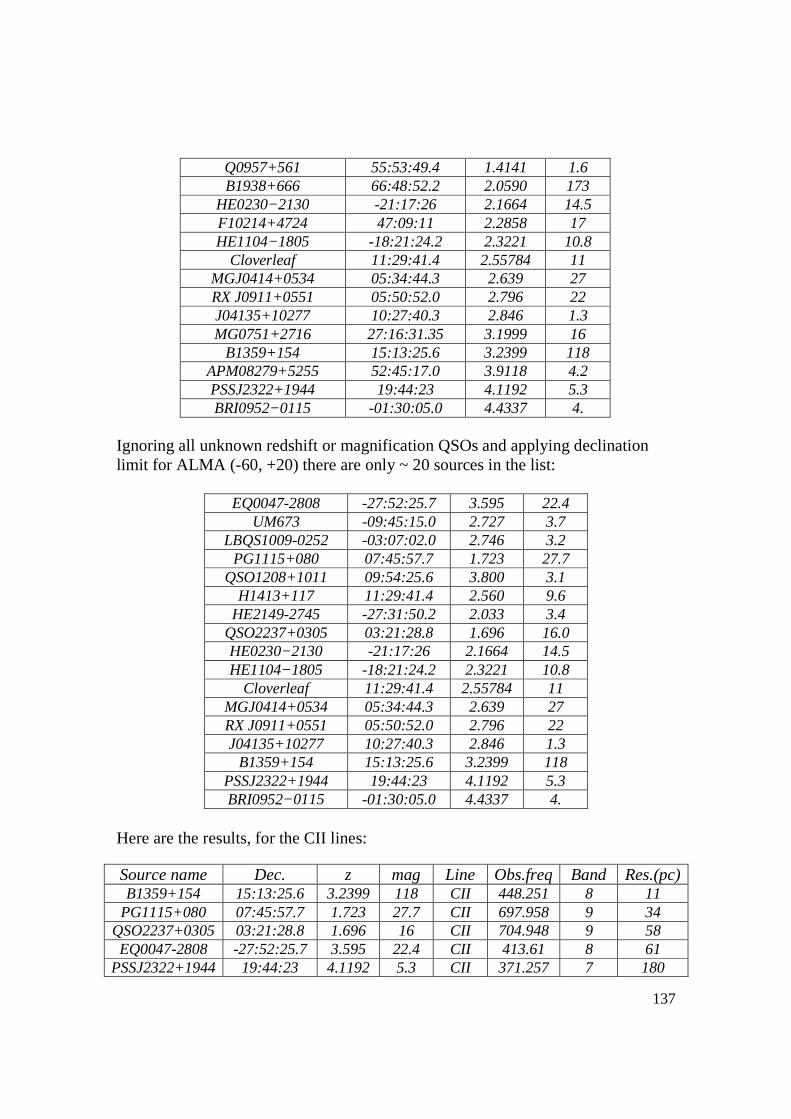
137

Q0957+561 55:53:49.4 1.4141 1.6 B1938+666 66:48:52.2 2.0590 173

HE0230−2130 -21:17:26 2.1664 14.5 F10214+4724 47:09:11 2.2858 17 HE1104−1805 -18:21:24.2 2.3221 10.8

Cloverleaf 11:29:41.4 2.55784 11 MGJ0414+0534 05:34:44.3 2.639 27 RX J0911+0551 05:50:52.0 2.796 22 J04135+10277 10:27:40.3 2.846 1.3 MG0751+2716 27:16:31.35 3.1999 16

B1359+154 15:13:25.6 3.2399 118 APM08279+5255 52:45:17.0 3.9118 4.2 PSSJ2322+1944 19:44:23 4.1192 5.3 BRI0952−0115 -01:30:05.0 4.4337 4.

Ignoring all unknown redshift or magnification QSOs and applying declination limit for ALMA (-60, +20) there are only ~ 20 sources in the list:

EQ0047-2808 -27:52:25.7 3.595 22.4 UM673 -09:45:15.0 2.727 3.7

LBQS1009-0252 -03:07:02.0 2.746 3.2 PG1115+080 07:45:57.7 1.723 27.7

QSO1208+1011 09:54:25.6 3.800 3.1 H1413+117 11:29:41.4 2.560 9.6

HE2149-2745 -27:31:50.2 2.033 3.4 QSO2237+0305 03:21:28.8 1.696 16.0 HE0230−2130 -21:17:26 2.1664 14.5 HE1104−1805 -18:21:24.2 2.3221 10.8

Cloverleaf 11:29:41.4 2.55784 11 MGJ0414+0534 05:34:44.3 2.639 27 RX J0911+0551 05:50:52.0 2.796 22 J04135+10277 10:27:40.3 2.846 1.3

B1359+154 15:13:25.6 3.2399 118 PSSJ2322+1944 19:44:23 4.1192 5.3 BRI0952−0115 -01:30:05.0 4.4337 4.

Here are the results, for the CII lines: Source name Dec. z mag Line Obs.freq Band Res.(pc) B1359+154 15:13:25.6 3.2399 118 CII 448.251 8 11

PG1115+080 07:45:57.7 1.723 27.7 CII 697.958 9 34 QSO2237+0305 03:21:28.8 1.696 16 CII 704.948 9 58 EQ0047-2808 -27:52:25.7 3.595 22.4 CII 413.61 8 61

PSSJ2322+1944 19:44:23 4.1192 5.3 CII 371.257 7 180

138

BRI0952-0115 -01:30:05.0 4.4337 4 CII 349.769 7 245 HE2149-2745 -27:31:50.2 2.033 3.4 CII 626.62 9 302

QSO1208+1011 09:54:25.6 3.8 3.1 CII 395.946 8 448 J04135+10277 10:27:40.3 2.846 1.3 CII 494.16 8 940

CO lines:

Source name Dec. z mag Line Obs.freq (GHz)

Band Res. (pc)

B1359+154 15:13:25.6 3.2399 118 CO(10-9) 271.701 6 12 B1359+154 15:13:25.6 3.2399 118 CO(9-8) 244.561 6 13

B1359+154 15:13:25.6 3.2399 118 CO(8-7) 217.411 6 15(15*118/31=57)

B1359+154 15:13:25.6 3.2399 118 CO(5-4) 135.915 4 24 (91) B1359+154 15:13:25.6 3.2399 118 CO(4-3) 108.739 3 30 (112)

PG1115+080 07:45:57.7 1.723 27.7 CO(8-7) 338.524 7 46 MGJ0414+0534 05:34:44.3 2.639 27 CO(10-9) 316.566 7 48

PG1115+080 07:45:57.7 1.723 27.7 CO(7-6) 296.236 7 53 MGJ0414+0534 05:34:44.3 2.639 27 CO(9-8) 284.944 7 53

PG1115+080 07:45:57.7 1.723 27.7 CO(10-9) 423.057 8 55 MGJ0414+0534 05:34:44.3 2.639 27 CO(8-7) 253.311 6 60 RX J0911+0551 05:50:52.0 2.796 22 CO(10-9) 303.474 7 61 PG1115+080 07:45:57.7 1.723 27.7 CO(6-5) 253.938 6 62 EQ0047-2808 -27:52:25.7 3.595 22.4 CO(10-9) 250.704 6 67

RX J0911+0551 05:50:52.0 2.796 22 CO(9-8) 273.159 6 67 MGJ0414+0534 05:34:44.3 2.639 27 CO(7-6) 221.669 6 69 EQ0047-2808 -27:52:25.7 3.595 22.4 CO(9-8) 225.661 6 74 PG1115+080 07:45:57.7 1.723 27.7 CO(5-4) 211.63 6 74

RX J0911+0551 05:50:52.0 2.796 22 CO(8-7) 242.834 6 76 QSO2237+0305 03:21:28.8 1.696 16 CO(8-7) 341.914 7 79 HE0230-2130 -21:17:26 2.1664 14.5 CO(10-9) 363.816 7 81

RX J0911+0551 05:50:52.0 2.796 22 CO(7-6) 212.5 6 87 (196) HE0230-2130 -21:17:26 2.1664 14.5 CO(9-8) 327.474 7 90

QSO2237+0305 03:21:28.8 1.696 16 CO(7-6) 299.203 7 91 QSO2237+0305 03:21:28.8 1.696 16 CO(10-9) 427.294 8 95 MGJ0414+0534 05:34:44.3 2.639 27 CO(5-4) 158.359 4 96 HE0230-2130 -21:17:26 2.1664 14.5 CO(8-7) 291.119 7 101

QSO2237+0305 03:21:28.8 1.696 16 CO(6-5) 256.481 6 106 EQ0047-2808 -27:52:25.7 3.595 22.4 CO(6-5) 150.484 4 111 HE1104-1805 -18:21:24.2 2.3221 10.8 CO(10-9) 346.764 7 112 HE0230-2130 -21:17:26 2.1664 14.5 CO(7-6) 254.754 6 115

Cloverleaf 11:29:41.4 2.55784 11 CO(10-9) 323.788 7 116 MGJ0414+0534 05:34:44.3 2.639 27 CO(4-3) 126.694 4 120 RX J0911+0551 05:50:52.0 2.796 22 CO(5-4) 151.809 4 121 PG1115+080 07:45:57.7 1.723 27.7 CO(3-2) 126.991 4 123 HE1104-1805 -18:21:24.2 2.3221 10.8 CO(9-8) 312.126 7 125

QSO2237+0305 03:21:28.8 1.696 16 CO(5-4) 213.749 6 127 Cloverleaf 11:29:41.4 2.55784 11 CO(9-8) 291.444 7 129

EQ0047-2808 -27:52:25.7 3.595 22.4 CO(5-4) 125.412 4 133 H1413+117 11:29:41.4 2.56 9.6 CO(10-9) 323.591 7 133

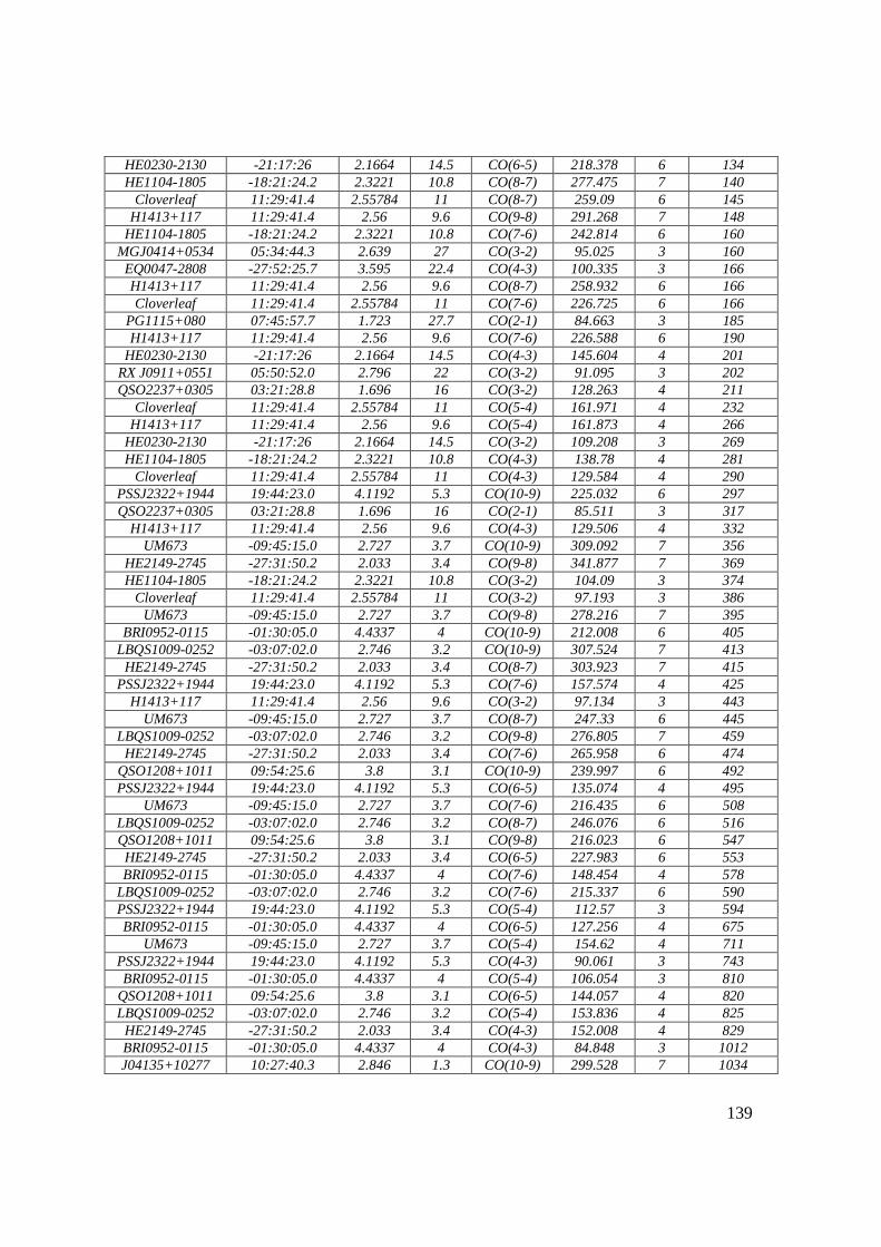
139

HE0230-2130 -21:17:26 2.1664 14.5 CO(6-5) 218.378 6 134 HE1104-1805 -18:21:24.2 2.3221 10.8 CO(8-7) 277.475 7 140

Cloverleaf 11:29:41.4 2.55784 11 CO(8-7) 259.09 6 145 H1413+117 11:29:41.4 2.56 9.6 CO(9-8) 291.268 7 148

HE1104-1805 -18:21:24.2 2.3221 10.8 CO(7-6) 242.814 6 160 MGJ0414+0534 05:34:44.3 2.639 27 CO(3-2) 95.025 3 160 EQ0047-2808 -27:52:25.7 3.595 22.4 CO(4-3) 100.335 3 166 H1413+117 11:29:41.4 2.56 9.6 CO(8-7) 258.932 6 166 Cloverleaf 11:29:41.4 2.55784 11 CO(7-6) 226.725 6 166

PG1115+080 07:45:57.7 1.723 27.7 CO(2-1) 84.663 3 185 H1413+117 11:29:41.4 2.56 9.6 CO(7-6) 226.588 6 190

HE0230-2130 -21:17:26 2.1664 14.5 CO(4-3) 145.604 4 201 RX J0911+0551 05:50:52.0 2.796 22 CO(3-2) 91.095 3 202 QSO2237+0305 03:21:28.8 1.696 16 CO(3-2) 128.263 4 211

Cloverleaf 11:29:41.4 2.55784 11 CO(5-4) 161.971 4 232 H1413+117 11:29:41.4 2.56 9.6 CO(5-4) 161.873 4 266

HE0230-2130 -21:17:26 2.1664 14.5 CO(3-2) 109.208 3 269 HE1104-1805 -18:21:24.2 2.3221 10.8 CO(4-3) 138.78 4 281

Cloverleaf 11:29:41.4 2.55784 11 CO(4-3) 129.584 4 290 PSSJ2322+1944 19:44:23.0 4.1192 5.3 CO(10-9) 225.032 6 297 QSO2237+0305 03:21:28.8 1.696 16 CO(2-1) 85.511 3 317

H1413+117 11:29:41.4 2.56 9.6 CO(4-3) 129.506 4 332 UM673 -09:45:15.0 2.727 3.7 CO(10-9) 309.092 7 356

HE2149-2745 -27:31:50.2 2.033 3.4 CO(9-8) 341.877 7 369 HE1104-1805 -18:21:24.2 2.3221 10.8 CO(3-2) 104.09 3 374

Cloverleaf 11:29:41.4 2.55784 11 CO(3-2) 97.193 3 386 UM673 -09:45:15.0 2.727 3.7 CO(9-8) 278.216 7 395

BRI0952-0115 -01:30:05.0 4.4337 4 CO(10-9) 212.008 6 405 LBQS1009-0252 -03:07:02.0 2.746 3.2 CO(10-9) 307.524 7 413 HE2149-2745 -27:31:50.2 2.033 3.4 CO(8-7) 303.923 7 415

PSSJ2322+1944 19:44:23.0 4.1192 5.3 CO(7-6) 157.574 4 425 H1413+117 11:29:41.4 2.56 9.6 CO(3-2) 97.134 3 443

UM673 -09:45:15.0 2.727 3.7 CO(8-7) 247.33 6 445 LBQS1009-0252 -03:07:02.0 2.746 3.2 CO(9-8) 276.805 7 459 HE2149-2745 -27:31:50.2 2.033 3.4 CO(7-6) 265.958 6 474

QSO1208+1011 09:54:25.6 3.8 3.1 CO(10-9) 239.997 6 492 PSSJ2322+1944 19:44:23.0 4.1192 5.3 CO(6-5) 135.074 4 495

UM673 -09:45:15.0 2.727 3.7 CO(7-6) 216.435 6 508 LBQS1009-0252 -03:07:02.0 2.746 3.2 CO(8-7) 246.076 6 516 QSO1208+1011 09:54:25.6 3.8 3.1 CO(9-8) 216.023 6 547 HE2149-2745 -27:31:50.2 2.033 3.4 CO(6-5) 227.983 6 553 BRI0952-0115 -01:30:05.0 4.4337 4 CO(7-6) 148.454 4 578

LBQS1009-0252 -03:07:02.0 2.746 3.2 CO(7-6) 215.337 6 590 PSSJ2322+1944 19:44:23.0 4.1192 5.3 CO(5-4) 112.57 3 594 BRI0952-0115 -01:30:05.0 4.4337 4 CO(6-5) 127.256 4 675

UM673 -09:45:15.0 2.727 3.7 CO(5-4) 154.62 4 711 PSSJ2322+1944 19:44:23.0 4.1192 5.3 CO(4-3) 90.061 3 743 BRI0952-0115 -01:30:05.0 4.4337 4 CO(5-4) 106.054 3 810

QSO1208+1011 09:54:25.6 3.8 3.1 CO(6-5) 144.057 4 820 LBQS1009-0252 -03:07:02.0 2.746 3.2 CO(5-4) 153.836 4 825 HE2149-2745 -27:31:50.2 2.033 3.4 CO(4-3) 152.008 4 829 BRI0952-0115 -01:30:05.0 4.4337 4 CO(4-3) 84.848 3 1012 J04135+10277 10:27:40.3 2.846 1.3 CO(10-9) 299.528 7 1034

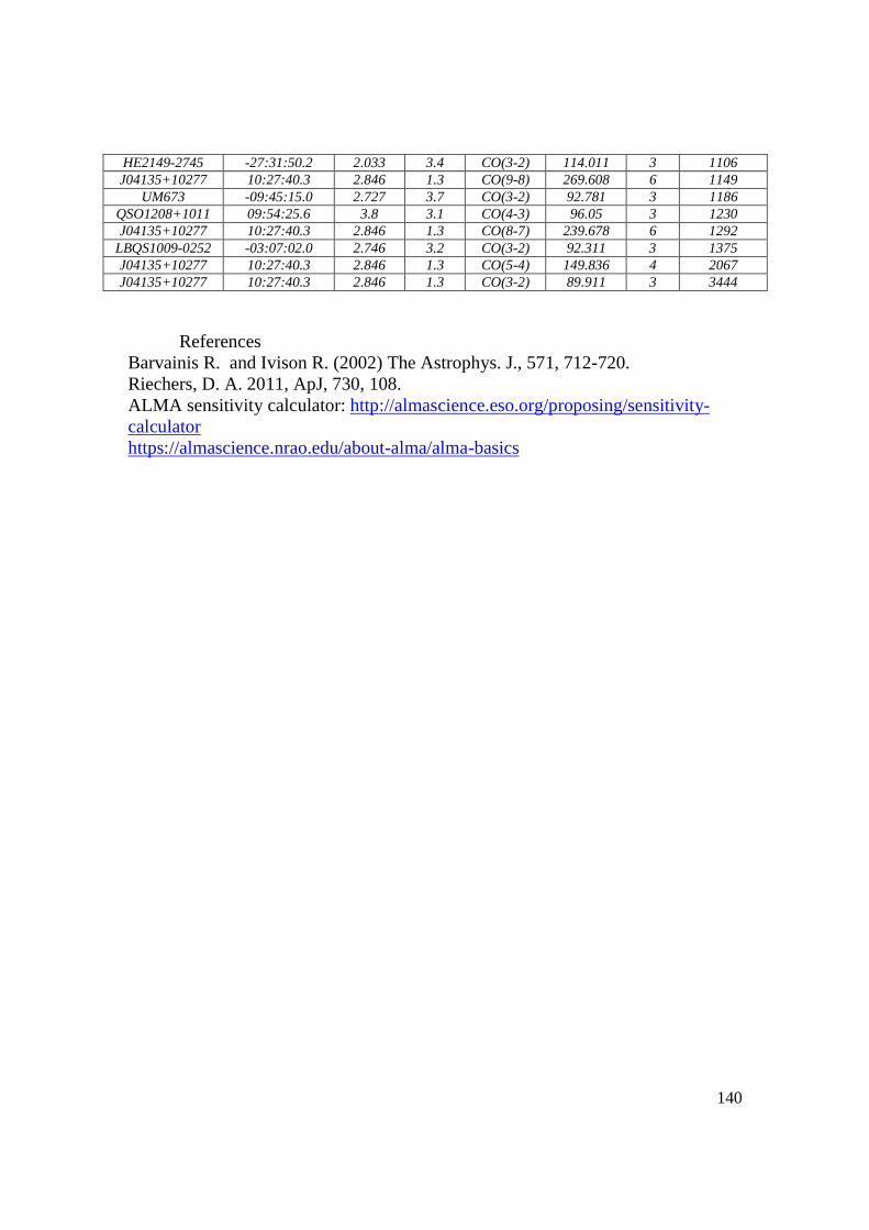
140

HE2149-2745 -27:31:50.2 2.033 3.4 CO(3-2) 114.011 3 1106 J04135+10277 10:27:40.3 2.846 1.3 CO(9-8) 269.608 6 1149

UM673 -09:45:15.0 2.727 3.7 CO(3-2) 92.781 3 1186 QSO1208+1011 09:54:25.6 3.8 3.1 CO(4-3) 96.05 3 1230 J04135+10277 10:27:40.3 2.846 1.3 CO(8-7) 239.678 6 1292

LBQS1009-0252 -03:07:02.0 2.746 3.2 CO(3-2) 92.311 3 1375 J04135+10277 10:27:40.3 2.846 1.3 CO(5-4) 149.836 4 2067 J04135+10277 10:27:40.3 2.846 1.3 CO(3-2) 89.911 3 3444

References Barvainis R. and Ivison R. (2002) The Astrophys. J., 571, 712-720. Riechers, D. A. 2011, ApJ, 730, 108. ALMA sensitivity calculator: http://almascience.eso.org/proposing/sensitivity-calculator https://almascience.nrao.edu/about-alma/alma-basics

141

A4. Proposal for observation at ALMA

50-pc resolution mapping of a unique strongly lensed z=3.24 QSO host galaxy

PI: Pham Tuan Anh and Frederic Boone 1 Abstract

We propose to map a molecular gas in the host galaxy of a gravitationally lensed quasar B1359+154, z = 3.24 with the spatial resolution up to 50 pc. For the time being, it is the best gravitationally lensed quasar that its host galaxy could be resolved with ALMA at that scale.

B1359+154 is a very rare, sextuply lensed quasar, lensed by a compact group including three primary lensing glaxies, which are situated on the vertices of a triangle, separated by ~ 0.7". Thanks to its source position which is very close to the lens caustic, its total magnification is very high, i.e. 118, (Barvanis and Ivison 2002) namely its image fluxes are magnified, up to a factor of 30 for the strongest one. It makes this quasar become one of the most promising object to observe at mm wavelength via the CO(9-8) molecular line.

With this observation we will be able to study the molecular gas disk morphology, its kinematics. Mapping a galaxy at redshift 3 with spatial resolution of 50 pc demonstrates a striking illustration of ALMA capabilities in term of both sensitivity and resolution. 2 General context

In the past decades submillimeter/millimeter (submm) observations of the interstellar medium in high-redshift (high-z) galaxies have opened a new window for studying the early Universe and the evolution of galaxies. In particular, continuum emission from dust heated by intense star formation (≥100 Msun yr−1 as well as large amounts of molecular gas 1010 Msun have been observed in quasi-stellar objects (QSOs) back to the end of the epoch of reionization (Carilli & Walter 2013). Simultaneously, a population of high-z galaxies dubbed submillimeter galaxies (SMGs) with similar molecular gas masses, star formation rates (SFR) and evolution have been discovered. Recent observations suggest a possible evolutionary link between these two populations. The large gas reservoirs observed in SMGs are supposed to be driven to the galaxy center, feeding intense starbursts and leading to the growth and activity of the central black holes that would become QSOs. The SMGs would thus transform into QSOs on a time-scale of ~100 Myr. If confirmed, this scenario would link the history of cosmic star formation with that of black hole growth, and it would give new insights into the role of feedback mechanisms in galaxy evolution. However, more detailed studies of individual galaxies are required to verify whether the morphologies and star-forming properties are consistent with this scenario.

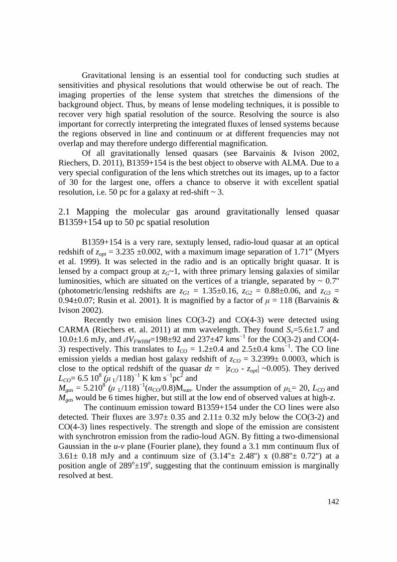
142

Gravitational lensing is an essential tool for conducting such studies at sensitivities and physical resolutions that would otherwise be out of reach. The imaging properties of the lense system that stretches the dimensions of the background object. Thus, by means of lense modeling techniques, it is possible to recover very high spatial resolution of the source. Resolving the source is also important for correctly interpreting the integrated fluxes of lensed systems because the regions observed in line and continuum or at different frequencies may not overlap and may therefore undergo differential magnification.

Of all gravitationally lensed quasars (see Barvainis & Ivison 2002, Riechers, D. 2011), B1359+154 is the best object to observe with ALMA. Due to a very special configuration of the lens which stretches out its images, up to a factor of 30 for the largest one, offers a chance to observe it with excellent spatial resolution, i.e. 50 pc for a galaxy at red-shift ~ 3. 2.1 Mapping the molecular gas around gravitationally lensed quasar B1359+154 up to 50 pc spatial resolution

B1359+154 is a very rare, sextuply lensed, radio-loud quasar at an optical redshift of zopt = 3.235 ±0.002, with a maximum image separation of 1.71” (Myers et al. 1999). It was selected in the radio and is an optically bright quasar. It is lensed by a compact group at zG~1, with three primary lensing galaxies of similar luminosities, which are situated on the vertices of a triangle, separated by ~ 0.7'' (photometric/lensing redshifts are zG1 = 1.35±0.16, zG2 = 0.88±0.06, and zG3 = 0.94±0.07; Rusin et al. 2001). It is magnified by a factor of µ = 118 (Barvainis & Ivison 2002).

Recently two emision lines CO(3-2) and CO(4-3) were detected using CARMA (Riechers et. al. 2011) at mm wavelength. They found Sv=5.6±1.7 and 10.0±1.6 mJy, and ∆VFWHM=198±92 and 237±47 kms−1 for the CO(3-2) and CO(4-3) respectively. This translates to ICO = 1.2±0.4 and 2.5±0.4 kms−1. The CO line emission yields a median host galaxy redshift of zCO = 3.2399± 0.0003, which is close to the optical redshift of the quasar dz = |zCO - zopt| ~0.005). They derived LCO= 6.5 108 (µ L/118)−1 K km s−1pc2 and Mgas = 5.2108 (µ L/118)−1(αCO/0.8)Msun. Under the assumption of µL= 20, LCO and Mgas would be 6 times higher, but still at the low end of observed values at high-z.

The continuum emission toward B1359+154 under the CO lines were also detected. Their fluxes are 3.97± 0.35 and 2.11± 0.32 mJy below the CO(3-2) and CO(4-3) lines respectively. The strength and slope of the emission are consistent with synchrotron emission from the radio-loud AGN. By fitting a two-dimensional Gaussian in the u-v plane (Fourier plane), they found a 3.1 mm continuum flux of 3.61± 0.18 mJy and a continuum size of (3.14''± 2.48'') x (0.88''± 0.72'') at a position angle of 289o±19o, suggesting that the continuum emission is marginally resolved at best.

143

B1359+154 gives 6 images (see Figure 1 (left)) in the visible range, which are named A, B, C, D, E, F. Mapping the molecular gas around this quasar requires both reliable lensing model and source model. Because of a special configuration of the lens, i.e. the source position respected to the lens caustic (see Figure 1 (right)), very similar to the case of RX J0911+0551, which we has reported recently in detail (Anh et. al. 2013, Do Thi Hoai et. al. 2013). We are able to map this source using the same method.

The relative brightness ratio between 6 images can be derived from Figure 1 (middle). A:B:C:D:E:F is 11:10:11:3:5:1. With a synthesis beam size ~ 0.2'' one may observe three blobs of images: A, B & C, and D & E & F. Namely, the peak relative brightness of three blobs A:BC:DEF is 11:10:5 or 2:2:1. It turns out that A image has the highest magnification factor, i.e. stretched most by the lensing, contributing to 11/(11+10+11+3+5+1) ~27% of total magnification 118 (Barvanis & Ivison 2002). We assume that the relative brightness ratio is the same at mm wavelength.

The resolution at 244.561 GHz (observed frequency of the molecular line CO(9-8)), for 1.5 km baseline is 0.207''. At redshift z = 3.24: 1'' corresponding to 7648.6 pc, namely the best resolution one can observe in the source plane is: 0.207*7648.6/(27%*118) ~ 50 pc.

2.2 A possibility to detect a water line

The main goal of this proposal is to map molecular gas around B1359+154 with very impressive resolution. However, since we use band 6 of ALMA to look at the CO(9-8) line, it is a bonus if we can detect the water line H2O(2-1) which is shifted to 233 GHz. There is a relation between H2O(2-1) and far-infrared luminosity (Omont et. al. 2013): LH2O(2-1)= LFIR

1.25 where LH2O(2-1) is in unit of 107Msun and LFIR in unit of 1012 Lsun. For B1359+154, LFIR = 0.093 1012Lsun therefore LH2O = 0.051 107Msun. The water line luminosity is computed (Carrili \& Walter 2013): LH2O = 1.0410−3SH2O∆VvobsDL

2. At z=3.24 DL=2.836 104 Mpc, ∆Vvobs~ 200 kms−1, vobs = 233.002 GHz, the estimated flux for A image (corrected for 27% of LH2O total flux): SH2O= 0.466 mJy. For 2 hours of observation, at the same observation condition as the CO(7-6) line, the noise at 233 GHz is 0.227 mJy, namely S/N = 0.466/0.227 ~ 2.

144

Figure 1. HST images of B1235+154 (left); radio spectra of its components, abscissa frequency in GHz, ordinate flux density in mJy (middle); best-fit model showing source position is at intersection of the dotted lines, very close to the caustic lens (right). (Rusin et. al. 2001).

Figure 2. Left and middle: CARMA CO(3-2) and CO(4-3) maps and spectra toward B1359+154 (Riechers 2011). Right: CO emission ladder of all sources where the CO(1-0) line has been measured (Carilli & Walter 2013)

2.3 Immediate objective: - Resolving the molecular gas around this quasar, its morphology and kinematics. - Resolving the dust emission under the observed lines towards this quasar. - A possibility to detect a water line from the host galaxy. 3 Potential for Publicity

For the time being, B1359+154 is the best gravitationally lensed quasar which its molecular gas could be spatially resolved up to 50 pc scale. Its map

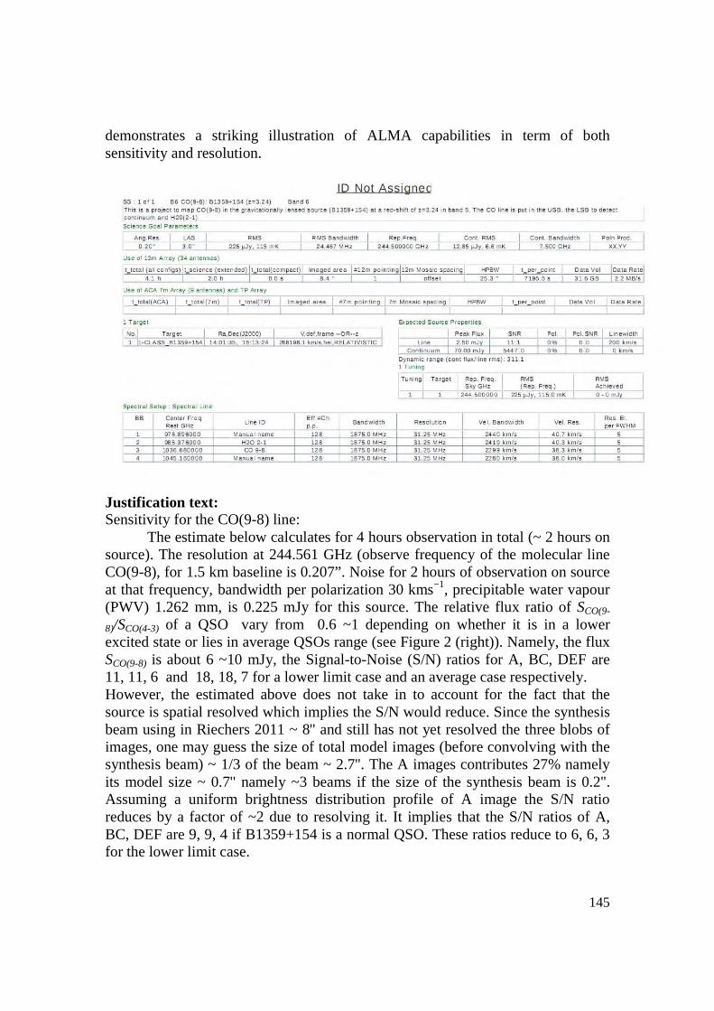
145

demonstrates a striking illustration of ALMA capabilities in term of both sensitivity and resolution.

Justification text: Sensitivity for the CO(9-8) line:

The estimate below calculates for 4 hours observation in total (~ 2 hours on source). The resolution at 244.561 GHz (observe frequency of the molecular line CO(9-8), for 1.5 km baseline is 0.207”. Noise for 2 hours of observation on source at that frequency, bandwidth per polarization 30 kms−1, precipitable water vapour (PWV) 1.262 mm, is 0.225 mJy for this source. The relative flux ratio of SCO(9-

8)/SCO(4-3) of a QSO vary from 0.6 ~1 depending on whether it is in a lower excited state or lies in average QSOs range (see Figure 2 (right)). Namely, the flux SCO(9-8) is about 6 ~10 mJy, the Signal-to-Noise (S/N) ratios for A, BC, DEF are 11, 11, 6 and 18, 18, 7 for a lower limit case and an average case respectively. However, the estimated above does not take in to account for the fact that the source is spatial resolved which implies the S/N would reduce. Since the synthesis beam using in Riechers 2011 ~ 8'' and still has not yet resolved the three blobs of images, one may guess the size of total model images (before convolving with the synthesis beam) ~ 1/3 of the beam ~ 2.7''. The A images contributes 27% namely its model size ~ 0.7'' namely ~3 beams if the size of the synthesis beam is 0.2''. Assuming a uniform brightness distribution profile of A image the S/N ratio reduces by a factor of ~2 due to resolving it. It implies that the S/N ratios of A, BC, DEF are 9, 9, 4 if B1359+154 is a normal QSO. These ratios reduce to 6, 6, 3 for the lower limit case.

146

Imaging: At ~ 240 GHz, the primary beam of 12 m antenna ~25”, the upper limit

scale of the source ~3” is well within 1/3 of it. References Carilli, C. & Walter, F. 2013, ARA&A, 51, 105, in press [arXiv:1301.0371]; Hoai, D. T. et al. 2013, RAA, [arXiv:1303.3707]; Anh, P. T. et al. A&A 552 L12 (2013); Barvainis, R. & Ivison, R. J. 2002, ApJ, 571, 712; Riechers, D. A. 2011a, ApJ, 730, 108 Rusin et. al. 2001,ApJ 557, 594; Omont et. al. 2013, A&A 551, 115;

147

List of Publications 1. P. T. Anh, F. Boone, D. T. Hoai, P. T. Nhung, A. Weiß, J.-P. Kneib, A. Beelen, P. Salomé, ‘Resolving the molecular gas around the lensed quasar RXJ0911.4+0551*’, A&A 552 L12 (2013), DOI: 10.1051/0004-6361/201321363 http://www.aanda.org/articles/aa/abs/2013/04/aa21363-13/aa21363-13.html 2. Do Thi Hoai, Pham Tuyet Nhung, Pham Tuan Anh, Frederic Boone, Pierre Darriulat, Pham Ngoc Diep, Pham Ngoc Dong, Nguyen Van Hiep, Nguyen Thi Thao, ‘Gravitationally lensed extended sources: the case of QSO RXJ0911’, Res. Astron. Astrophys. Vol 13, No 7 (2013), DOI: 10.1088/1674-4527/13/7/004 http://iopscience.iop.org/1674-4527/13/7/004/

Résumé

Nous présentons une étude détaillée d’observations faites de la galaxie hôte d’un quasar lointain (z~2.8), RX J0911. La détection de l’émission des molécules CO a été possible grâce au lentillage gravitationnel dû à la présence d’une galaxie plus proche sur la ligne de vue et à la qualité de l’interféromètre du Plateau de Bure. On a obtenu de très bonnes résolutions tant en fréquence, permettant une mesure précise de la largeur de raie, qu’en direction, permettant de résoudre la source aussi bien sur la raie que dans le continu, donc à la fois pour le gaz et pour la poussière. Nous avons discuté en détail le mécanisme de lentillage gravitationnel. Comme souvent lorsqu’il s’agit de grandissements importants, la source est proche de la caustique de la lentille, dans le cas précis elle la chevauche. Il en résulte une dépendance importante du grandissement sur la position précise des sources ponctuelles à l’intérieur de la galaxie, donc des grandissements différents pour le gaz, la poussière et le quasar. D’autre part, les images sont non seulement aggrandies mais aussi déformées. Les données illustrent les avantages offerts par le lentillage en termes de sensibilité en même temps que les complications de l’analyse qui en découlent, source d’incertitudes sur les mesures. La raie CO(7-6) sort clairement du continu, permettant des mesures fiables des luminositées associées au gaz et à la poussière. Des études détaillées des quatre images ont permis de résoudre la source tant sur la raie que dans le continu, avec des rayons de 106±15 et 39±18 mas respectivement. Dans le cas de la raie, la qualité des données a permis de mettre en évidence une excentricité à 3.3 déviations standard et un gradient de vitesse à 4.5 déviations standards. La largeur très étroite de la raie implique une masse dynamique basse et les évaluations faites des masses de gaz et de poussière sont elles aussi très au dessous de ce qu’on mesure généralement pour des quasars à fort décalage vers le rouge. La valeur élevée de l’efficacité de formation d’étoiles situe la galaxie dans la partie haute de la distribution des galaxies, qu’elles soient à haut ou bas z: une fraction importante du volume gazeux semble avoir été épuisée à la suite d’une période de formation d’étoiles intense, laissant la galaxie à la frontière des galaxies hôtes de quasar à haut et bas z.

Abstract

The thesis gives a detailed account of observations of the host galaxy of a distant quasar, RX J0911. Detailed observations of the CO emission have been made possible thanks to the gravitational lensing offered by the presence of a galaxy in the foreground and to the quality of the Plateau de Bure Interferometer. High resolutions have been obtained both in frequency, allowing for a precise measurement of the line width, and in space, allowing for resolving spatially the source both on the line and in the continuum, namely both in its dust and gas content. The mechanism of gravitational lensing has been discussed in detail. As is often the case with large magnifications, the source happens to be in the vicinity of the lens caustic, in fact to overlap it. A consequence is a strong dependence of the magnification on the precise position of point sources in the galaxy, resulting in significantly different magnifications for the gas, the dust and the central QSO. Moreover, the morphology of the observed images is distorted in addition to being amplified. The data illustrate the advantage offered by the strong lensing in terms of increased sensitivity as well as the complication that results, causing an additional source of uncertainties on the quantities that are accessible to measurement. The CO(7-6) line stands out clearly above continuum, allowing for reliable measurements of the gas and dust luminosities. Detailed studies of the four lensed images have made it possible to resolve the source in both the line and the continuum with rms radii of 106±15 and 39±18 mas respectively. In the line case, the quality of the data have provided evidence for an ellipticity of the source, 3.3 standard deviations away from circular, and for a velocity gradient correlated with the source ellipticity, at the level of 4.5 standard deviations. The very narrow CO(7-6) line implies a low dynamical mass and both gas and dust mass evaluations fall on the low side of the normal high-z quasar host population. The large star formation efficiency is on the high side of both low-z and high-z galaxies: much of the gas has been exhausted after an intense star formation period, leaving the galaxy at the border between high-z and low-z quasar hosts.