T-47 Final Report

1

FINAL PERFORMANCE REPORT

South Carolina State Wildlife Grant T-47-R

October 1, 2009 – December 22, 2011

TITLE: Conservation of Breeding Painted Buntings and Other Songbird Indicators in Early-

successional Shrub-scrub Habitat

GRANT OBJECTIVES

1. Determine breeding bird abundance in paired CP-33 (treatment) and non-CP-33 (control)

fields for Painted Bunting and other indicator songbird species.

2. Determine nest location and success of Painted Buntings in paired CP-33 and non-CP-33

fields.

3. Develop a landscape/GAP analysis model to track dynamic seasonal crop rotation and

predict the pattern of habitat occupancy and breeding distribution of Painted Bunting as

well as associated early-successional shrub-scrub songbird indicator species (i.e., Indigo

Bunting and Blue Grosbeak).

ACTIVITY OVERVIEW:

Activities associated with the grant are described below, according to the original tasks and

subtasks in the Project Statement for this grant.

Tasks

I. Determine breeding bird abundance in paired CP-33 (treatment) and non-CP-33 (control)

fields for Painted Bunting and other indicator songbird species.

Activity: Eight fields were used as intensive study sites (4 treatments and 4 controls).

Habitat types at the sites were classified as follows: agriculture, forest, CP-33 border, and

cut. “Cut” referred to a recently cut forest area. On each field, spot maps, transects and

radio telemetry data were taken to assess Painted Bunting abundance. Data on other

indicator songbird species were gathered using spot maps and transects.

Spot maps were performed at varying times between sunrise and sunset. Each field

received at least 6 visits per field season. Each sighting for Painted Buntings, Blue

Grosbeaks, and Indigo Buntings was marked on a map for approximate location along

with its sex and any behavior it might be exhibiting (singing, fighting, chipping).

Transect counts were performed on each site every 2 weeks. Each was 200m long and

ran along the edge of the field, typically bordering a forested edge. These were all

completed between sunrise and 10am. All bird species seen or heard were noted along

with its approximate distance and bearing from the observer. Observers were to remain

along transects for a minimum of 20 minutes.

Telemetry was carried out on Painted Buntings only. Twenty three (23) transmitters were

applied between the 2009 and 2010 field seasons. Tagged birds were tracked each day

and location of first sighting was taken with a handheld GPS unit. Other data such as

bird height, perch species, bird behaviors, time, weather, and vegetation data were taken

along with each GPS point.

T-47 Final Report

2

Vegetation data were also gathered in the forested edges of agricultural fields, in the CP-

33 strips, and in the crop fields themselves. The procedure used for this was based on the

BBIRD (Breeding Biology Research & Monitoring Database. Montana Coop. Wildlife

Research Unit. 1997) field protocol; it was simplified due to time/personnel constraints.

A set of systematically chosen vegetation plots were measured two times in 2009 and two

times in 2010. The same type of vegetation data was gathered at each telemetry point

gathered on individual Painted Buntings.

Data Analysis: Our transect data reveal no significant difference between numbers of

birds detected on treatments vs. controls (based on independent samples T-Test: t(2)= -

0.701, p = 0.556). However, we did have significantly more detections of birds within

mature (>= 10 years of growth) forest edges compared to detections within immature

forest edges (<= 10 years of growth; labeled ‘Cut’ below), CP-33 strips, and cropland

(ANOVA: F(3,7) = 79.649, p= 0.001).

Transect Bird Detections (All species)

2009 2010

Forest 390* 341*

Ag 59 48

CP-33 42 23

Cut 34 81

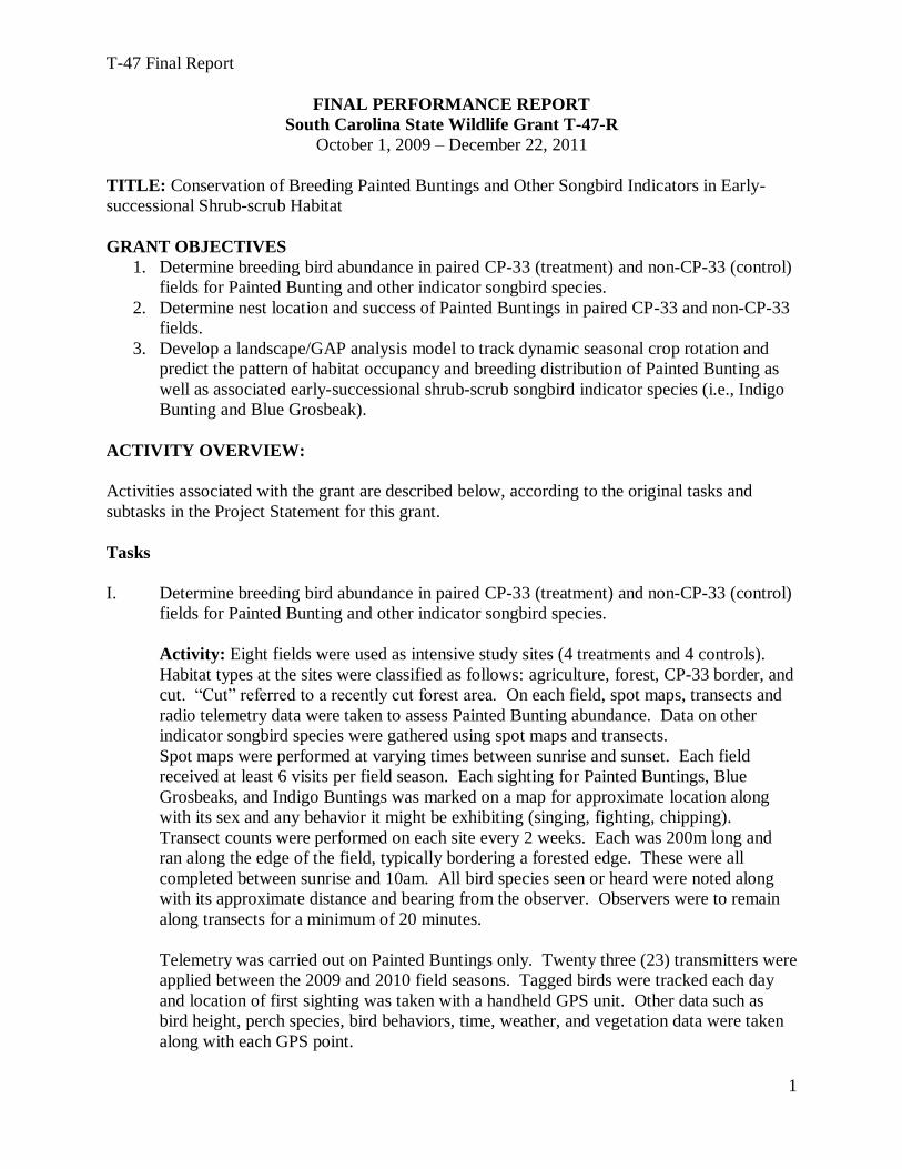
The following pages list the bird species detected on transects in control and treatment

sites respectively.

T-47 Final Report

3

Count of Bird Species on Controls

Species Scientific Name Count %

Indigo Bunting Passerina cyanea 65 19.52

Northern Cardinal Cardinalis cardinalis 44 13.21

Painted Bunting Passerina ciris 43 12.91

Blue Grosbeak Passerina caerulea 35 10.51

Mourning Dove Zenaida macroura 15 4.5

Carolina Wren Thryothorus ludovicianus 12 3.6

Blue Jay Cyanocitta cristata 11 3.3

Eastern Towhee Pipilo erythrophthalmus 11 3.3

White-Eyed Vireo Vireo griseus 8 2.4

Blue-Gray Gnatcatcher Polioptila caerulea 7 2.1

Red-Bellied Woodpecker Melanerpes carolinus 7 2.1

Northern Bobwhite Quail Colinus virginianus 6 1.8

Common Yellowthroat Geothlypis trichas 5 1.5

Tufted Titmouse Baeolophus bicolor 5 1.5

Orchard Oriole Icterus spurius 5 1.5

Yellow-Breasted Chat Icteria virens 5 1.5

Yellow-Billed Cuckoo Coccyzus americanus 5 1.5

American Crow Corvus brachyrhynchos 4 1.2

Brown-Headed Cowbird Molothrus ater 4 1.2

Eastern Bluebird Sialia sialis 4 1.2

Eastern Kingbird Tyrannus tyrannus 4 1.2

Fish Crow Corvus ossifragus 4 1.2

Purple Martin Progne subis 4 1.2

Brown Thrasher Toxostoma rufum 2 0.6

Carolina Chickadee Poecile carolinensis 2 0.6

Great Crested Flycatcher Myiarchus crinitus 2 0.6

Northern Flicker Colaptes auratus 2 0.6

Northern Parula Parula americana 2 0.6

Red-Eyed Vireo Vireo olivaceus 2 0.6

Summer Tanager Piranga rubra 2 0.6

Common Grackle Quiscalus quiscula 1 0.3

Hooded Warbler Wilsonia citrina 1 0.3

Loggerhead Shrike Lanius ludovicianus 1 0.3

Red-Headed Woodpecker Melanerpes erythrocephalus 1 0.3

Ruby-Throated Hummingbird Archilochus colubris 1 0.3

Red-Winged Blackbird Agelaius phoeniceus 1 0.3

Totals 36 species 333 individuals

T-47 Final Report

4

Count of Bird Species on Treatments

Species Scientific Name Count %

Indigo Bunting Passerina cyanea 70 18.13

Blue Grosbeak Passerina caerulea 51 13.21

Northern Cardinal Cardinalis cardinalis 37 9.59

Painted Bunting Passerina ciris 31 8.03

Mourning Dove Zenaida macroura 19 4.92

Northern Bobwhite Quail Colinus virginianus 17 4.4

Blue-Gray Gnatcatcher Polioptila caerulea 13 3.37

Carolina Wren Thryothorus ludovicianus 13 3.37

Eastern Towhee Pipilo erythrophthalmus 13 3.37

Tufted Titmouse Baeolophus bicolor 11 2.85

Red-Eyed Vireo Vireo olivaceus 10 2.59

White-Eyed Vireo Vireo griseus 9 2.33

Orchard Oriole Icterus spurius 8 2.07

Red-Bellied Woodpecker Melanerpes carolinus 8 2.07

Blue Jay Cyanocitta cristata 6 1.55

Carolina Chickadee Poecile carolinensis 6 1.55

Summer Tanager Piranga rubra 6 1.55

Yellow-Breasted Chat Icteria virens 5 1.3

Yellow-Billed Cuckoo Coccyzus americanus 5 1.3

American Crow Corvus brachyrhynchos 4 1.04

Brown-Headed Cowbird Molothrus ater 4 1.04

Common Grackle Quiscalus quiscula 4 1.04

Northern Parula Parula americana 4 1.04

Pileated Woodpecker Dryocopus pileatus 4 1.04

Common Yellowthroat Geothlypis trichas 3 0.78

Downy Woodpecker Picoides pubescens 3 0.78

Eastern Bluebird Sialia sialis 3 0.78

Eastern Kingbird Tyrannus tyrannus 2 0.52

Great Crested Flycatcher Myiarchus crinitus 2 0.52

Northern Mockingbird Mimus polyglottos 2 0.52

Red-Winged Blackbird Agelaius phoeniceus 2 0.52

Brown Thrasher Toxostoma rufum 1 0.26

Fish Crow Corvus ossifragus 1 0.26

Field Sparrow Spizella pusilla 1 0.26

Gray Catbird Dumetella carolinensis 1 0.26

Hooded Warbler Wilsonia citrina 1 0.26

Northern Flicker Colaptes auratus 1 0.26

Pine Warbler Dendroica pinus 1 0.26

Purple Martin Progne subis 1 0.26

Red-Tailed Hawk Buteo jamaicensis 1 0.26

Ruby-Throated Hummingbird Archilochus colubris 1 0.26

Wood Thrush Hylocichla mustelina 1 0.26

T-47 Final Report

5

Totals 42 species 386 individuals

A high volume of avian detections within forest edges vs. other habitat types was also

reflected in our spot map data. The following table includes all spot map data for Painted

Bunting (PABU), Indigo Bunting (INBU), and Blue Grosbeak (BLGR) (ANOVA:

F(3,7)= 14.310, p= 0.013). A graphical representation of these data is given following

the table. This table should be interpreted with caution however; in terms of area

surveyed, agriculture was number one with the most area, then forest, and CP-33 and Cut

had the least total area.

Spot Map Bird Detections (PABU, INBU, BLGR)

2009 2010

Forest 496* 537*

Ag 87 218

CP-33 62 109

Cut 55 207

Our telemetry data again reflect the same pattern of habitat use (ANOVA: F(3,7)=

19.874, p= 0.007).

0

50

100

150

200

250

300

Bir

d R

aw N

um

ber

s

Spot Map Bird Detections (PABU, INBU, BLGR)

2010

2009

PABU INBU BLGR

T-47 Final Report

6

Telemetry Bird Detections (PABU)

2009 2010

Forest 146* 122*

Ag 25 67

CP-33 15 9

Cut 8 23

Important vegetation characteristics for Painted Bunting were determined for croplands,

CP-33/immature forest edges (<= 10 years of growth), and mature forest edges (>= 10

years of growth) using a statistical technique called binary logistic regression. The

following is a table of the forest variables gathered, their statistical significance, and

other variables that will be explained below the table.

Forest Variables and Statistics

Sig. Exp(B) 95.0% C.I.for

EXP(B)

Lower Upper

% Green .341 1.008 .992 1.023

% Grass/Sedge .409 1.012 .984 1.040

% Shrub .897 1.001 .982 1.021

% Brush .756 .997 .979 1.015

% Forb .482 .995 .980 1.010

% Leaf Litter .737 1.003 .988 1.018

% Fallen Log .012* .868 .777 .970

% Bare Ground .638 .989 .943 1.036

Total Average Plant Height .001** .805 .710 .913

% Cover Woody Plants 0.5-8m .930 .999 .984 1.015

Average Height Vegetation 0.5-8m .027* 1.225 1.024 1.466

% Cover Woody Plants >8m .274 .991 .974 1.007

Average Height Vegetation >8m .000** 1.179 1.078 1.289

# Snags .035* 1.451 1.027 2.049

# Trees 8-23 cm dbh .031* 1.028 1.003 1.054

# Trees 23-38 cm dbh .033* 1.132 1.010 1.269

# Trees >38 cm dbh .351 .878 .668 1.154

Interpreting statistics: The ‘Sig.’ column stands for significance or p value. Items with a

single star are significant to the p < 0.05 level (statistically significant) and items with a

double star are significant to the p < 0.01 level (very statistically significant). The

Exp(B) column is only important for values that are statistically significant. These values

tell you how much of an increased or decreased likelihood of finding a Painted Bunting

T-47 Final Report

7

in a vegetation plot for each unit increase of the variable. Values greater than 1 show an

increased likelihood in finding a Painted Bunting on a vegetation plot with every unit

increase of the variable, whereas values less than 1 show a decreased likelihood of

finding a Painted Bunting on a vegetation plot with every unit increase of the variable.

To interpret these values, it is necessary to translate them into percents. To do this,

subtract 1 from the value, and multiply this value by 100. For example, for the variable

‘# Trees 8-23 cm dbh’, subtracting 1 from 1.028 gives you 0.028. Multiplying this by

100 gives you 2.8. So for every unit increase in this variable (each additional tree 8-23

cm dbh) on a vegetation plot, there is a 2.8% increased likelihood of finding a Painted

Bunting. As another example, look at the ‘% Fallen Log’ variable. Subtracting 1 from

0.868 gives you -0.132. Multiply this by 100 to get -13.2. This means for each extra

percentage increase in fallen log within a vegetation plot, there is a 13.2% decreased

likelihood of finding a Painted Bunting.

Vegetation data gathered on CP-33 strips was gathered in the same manner as the forest

vegetation data; however the variables on tall vertical woody components were

eliminated (because they didn’t exist). The table below summarizes these data. It should

be interpreted in the same manner as the Forest Variables and Statistics table above (see

Interpreting Statistics section immediately following that table).

CP-33/Grassland Variables and Statistics

Sig. Exp(B) 95.0% C.I.for

EXP(B)

Lower Upper

% Green .103 1.043 .992 1.096

% Grass/Sedge .018* .953 .916 .992

% Shrub .002** 1.152 1.055 1.259

% Brush .102 .930 .853 1.014

% Forb .050 .961 .923 1.000

% Leaf Litter .887 1.001 .985 1.018

% Bare Ground .370 .986 .956 1.017

Total Average Plant Height .124 1.816 .850 3.880

Vegetation data gathered in the field reveal wheat is the Painted Bunting’s crop of choice

by far. An omnibus test was used and the results are in the following table. They can be

interpreted the same way as the two vegetation tables above.

Crop Type Preference in PABU and Statistics

Reference

category

Sig. Exp(B) 95.0% C.I.for EXP(B)

Lower Upper

Wheat vs. Soy Soy .002** 6.419 1.941 21.230

Corn vs. Soy Soy .810 1.245 .208 7.433

Wheat vs. Corn Corn .028* 5.157 1.194 22.273

T-47 Final Report

8

These data show Painted Buntings were 6.419 times more likely to be found in wheat

than soy, and 5.157 times more likely to be found in wheat than corn.

Significant deviations: None.

II. Determine nest location and success of Painted Buntings in paired CP-33 and non-CP-33

fields.

Activity: Painted Bunting nests were searched in three fields, one paired CP-33 and non-

CP-33 field and a field managed by SCDNR for doves (hereby referred to as the “Dove

Field”). The Dove Field was included in our monitoring efforts as many of the same

characteristics as the CP-33 fields were present at this site as well as other management

techniques. Again, we followed the BBIRD protocols, this time for nest monitoring (see

BBIRD reference above). Briefly, fields were searched for nests during daylight hours in

all habitat types at each of our three nest monitoring sites. Once a nest was found, the

species was determined, and monitoring began. So as not to disturb the nest, located

nests were visited every 2-3 days to observe and count the number of eggs in the nest,

and then to observe when the eggs hatched. After hatching, the nestlings were monitored

until they fledged the nest, Brown-headed Cowbirds parasitized the nest, or predators ate

the nestlings. Some of the fledglings were banded so that if monitoring was continued in

future years (beyond the scope of this study), those birds could be accounted for. It

should be noted that due of the amount of work completed in years 1 and 2 for objectives

1 and 3, a shortage of personnel, and the amount of effort necessary for nest monitoring,

this objective for nest location and success was set aside as a unique and only task for

year 3. This justification follows the guidelines of the work to be completed, as year 3

was planned as a “follow-up” season to tie-up loose ends or anything else that needed to

be completed.

Data Summary: A total of 22 Painted Bunting nests were found and monitored among

the three sites. Monitoring began in June 2011 and concluded at the end of July 2011.

This compares to only a total of five nests found by causal observations during years 1

and 2. Of the 22 nests, 10 nests successfully fledged young (45.5%), 6 nests had an

unknown fate (27.3%), 5 nests failed (22.7%), and a Brown-headed Cowbird parasitized

one nest (4.5%). These numbers and the percent of the total are summarized in the table

below.

Category Number Percent

Fledged nests 10 45.5

Unknown fate 6 27.3

Failed nests 5 22.7

Parasitized 1 4.5

Total nests 22 -

T-47 Final Report

9

A nest with an unknown fate was one in which the eggs or fledglings disappeared

between observation days. It is impossible to know the reasons for either the nests that

failed or the nests of unknown fate, but possibilities include predation, sever weather

from storms, and/or abandonment. Though this represents only a small sample of nests in

a two-county area, these percentages do not bode well for Painted Buntings. More than

half of the nests monitored were not successful (54.5% when the non-fledged categories

are combined). One surprising finding was that all nests were located in forest-edge

habitat and none were found in CP-33 habitat or similar management within the Dove

Field. Painted Buntings are known to prefer nesting sites in low shrubs (4-5 feet) and 3

nests were found at this level; however, most nests were found as high as 10-15 feet (3.1-

4.6 meters) off the ground. If Painted Buntings in this area are dependent upon these

forest edges for nesting sites and not CP-33, then management should consider this

habitat as one of high conservation value based upon this and the findings in the next

section (below).

Significant deviations: None

III. Develop a landscape/GAP analysis model to track dynamic seasonal crop rotation and

predict the pattern of habitat occupancy and breeding distribution of Painted Bunting as

well as associated early-successional shrub-scrub songbird indicator species (i.e., Indigo

Bunting and Blue Grosbeak).

Activity: A landscape/GAP analysis map was created specifically for Painted Buntings

based on data gathered through the following surveys: spot maps, transect counts, and

radio telemetry. The spatial data used to generate this landscape/GAP analysis map was

a NOAA C-Cap Regional Land Cover data map from the following website:

http://www.csc.noaa.gov/digitalcoast/data/index.html . This map was based on data from

Landsat satellites. It was chosen because it was already classified into habitat types. The

23 habitat types that came with this map were simplified to 6 for the purpose of this

project: development (towns, suburban residences, and roads), cropland,

grassland/shrub/scrub (this includes CP-33), forest (this includes the wetland habitat type

since any wetlands bordering our study sites were highly wooded), open water, and bare

land. Information on Painted Buntings gathered in the field was added to determine high

priority habitat. The criteria for high priority habitat are as follows:

Forest habitats 25m or less from nearest edge.

CP-33 strips, wheat fields, and early growth forests (<=10 years of growth)

were anecdotally observed to harbor grasses and insects Painted Bunting were

eating. This is the suspected reason there were more detections of Painted

Bunting in wheat fields than soy or corn fields.

Use of CP-33, all agricultural fields, and early growth forests was also limited

to the edges of these habitats.

For reasons that will be explained in the ‘Words of Caution about this map’ section, a

medium priority habitat category was added to the map. Based on our data, the combined

accuracy of the map including high priority habitat and medium priority habitat is

97.31%.

T-47 Final Report

10

T-47 Final Report

11

Words of Caution about this map: Since the original NOAA C-CAP map was based on

Landsat data, the spatial resolution of this map is 30m x 30m. Painted Buntings however,

were observed no further from forest edges than 25m. Therefore, any edge habitat

included in the high priority category of the landscape/GAP analysis map was 30m wide.

At first glance then, it would seem that the high priority habitat map category would be

an overestimate of Painted Bunting distribution. However, due to the low resolution

nature of Landsat data, many of the thin forest strips that were essential for individuals

were missed. It is for this reason that the ‘medium priority’ category was added. This

category includes all of the thin forest strips on our sites that were previously missed in

the high priority category as well as all cropland.

Below is an illustrated example of this resolution problem. The first image is a section of

1m x 1m resolution aerial photo obtained for one of the study sites. The small bright

green dots represent GPS points obtained on a male Painted Bunting in 2009. Another

individual occupied this same territory in 2010. The second image is the same area as

described by the landscape/GAP analysis map. The same color convention exists in this

picture as the large map above. Notice how the thin forest segment where this individual

spent most of his time was not included in the high priority (red) area due to low

resolution, but was picked up using the medium priority area (yellow).

Areal Photo GAP Analysis Map

The following is a measure of approximate accuracy for the landscape/GAP analysis

based on these differences between high and medium priority areas:

Habitat Category Estimated Accuracy of landscape/GAP analysis map

Developed Underestimated by 2.31%

T-47 Final Report

12

Cropland Overestimated by 22.52%

CP-33/Grassland Underestimated by 9.70%

Forest Underestimated by 10.56%

Open Water Overestimated by 0.04%

Bare Ground No data from study sites

Notes on seasonal crop rotation: The 3 crops observed on study sites for this project were

wheat, soy, and corn. Three patterns of crop rotation occurred within this context.

1. Fields that started with wheat at the beginning of the field season (May) switched to

either corn or soy halfway through the field season (late May, June).

2. Fields that started in corn stayed corn throughout the field season. A small number of

fields were harvested the last few of days in the field season (July 30- August 1).

3. Fields that started in soy remained soy throughout the field season. No observation of

a soy harvest was made.

There were only 2 observations of territory shifts throughout the field season out of 23

Painted Bunting individuals who were followed using telemetry. It is suspected that the

majority of individuals establish territories based on the state of the landscape- including

crops planted- in April/May and stay regardless of what happens later in the breeding

season.

Notes on INBU and BLGR: Data were gathered for these species using spot maps and

transect counts. Data suggest similar habitat use to PABU in both cases, however the

addition of telemetry data are needed as individuals may tend to have higher detections in

habitats where they are either highly visible, highly vocal, or both; possibly going

undetected in other areas.

Our Recommendations: The following are general recommendations for Painted Bunting

conservation for rural central South Carolina:

Mature forest edges (>= 10 years old) are of utmost importance

PABU occupy and nest in the outermost edge of forests and/or thin forest

strips; 25m or less from the edge

A source of food in the form of a wheat field or other grass seed as well as a

source of insects when rearing young is also necessary

Significant deviations: None.

Estimated Federal Expenditure (grant level): $89,854

Recommendations: Use the information gathered to make sound decisions about habitat

protection and management.