final focus layouts and stability considerations · cas 2018, a. seryi, jai 2 we will focus here on...

Final Focus Layouts and Stability Considerations

Andrei SeryiJohn Adams Institute

CERN Accelerator SchoolBeam dynamics and technologies for future colliders

March 2018, Zurich

CAS 2018, A. Seryi, JAI 2

We will focus here on final focus design

As FF most challenging for linear colliders, we will first consider FF of LCs

We will then touch on stability issues of FFs of LCs

And then discuss design of FF in modern hadron or e+e- circular colliders


International Linear Collider ILC

ILC e+e- Linear Collider

Energy 250 GeV x 250 GeV


• Energy – need to reach at least 250 GeV CM

• Luminosity – need to reach 10^34 level

Linear Collider – two main challenges


The Luminosity Challenge • Must jump by a Factor of

10000 in Luminosity !!!(from what is achieved in the only so far linear collider SLC)

• Many improvements, to ensure this : generation of smaller emittances, their better preservation, …

• Including better focusing, dealing with beam-beam, safely removing beams after collision and better stability

at SLC


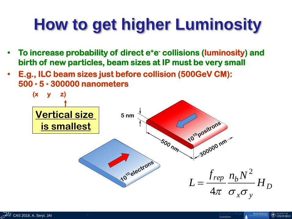
How to get higher Luminosity

• To increase probability of direct e+e- collisions (luminosity) and

birth of new particles, beam sizes at IP must be very small

• E.g., ILC beam sizes just before collision (500GeV CM):

500 * 5 * 300000 nanometers

(x y z)

Vertical size

is smallest

Dyx

brepH

NnfL

2

4

5 nm


BDS: from end of linac to IP, to dumps

Beam Delivery System (BDS)It includes FF, and many other systems


Beam Delivery subsystems

14mr IR

Final FocusE-collimator

b-collimator

Diagnostics

Tune-up

dump

Beam

Switch

YardSacrificial

collimators

Extractiongrid: 100m*1m Main dump

Muon wall

Tune-up &

emergency

Extraction

• As we go through the lecture, the purpose of each subsystem should

become clear


Beam Delivery System tasks

• measure the linac beam and match it into the final focus

• remove any large amplitude particles (beam-halo) from the linac to minimize background in the detectors

• measure and monitor the key physics parameters such as energy and polarization before and after the collisions

• ensure that the extremely small beams collide optimally at the IP

• protect the beamline and detector against mis-steered beams from the main linacs and safely extract them to beam dump

• provide possibility for two detectors to utilize single IP with efficient and rapid switch-over


Parameters of ILC BDS


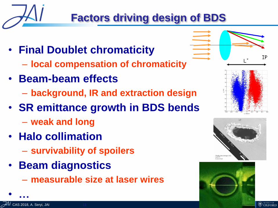
Factors driving design of BDS

• Final Doublet chromaticity

– local compensation of chromaticity

• Beam-beam effects

– background, IR and extraction design

• SR emittance growth in BDS bends

– weak and long

• Halo collimation

– survivability of spoilers

• Beam diagnostics

– measurable size at laser wires

• …


How to focus the beam to a smallest spot?

• If you ever played with a lens trying to burn a picture on a wood under bright sun, then you know that one needs a strong and big lens

• It is very similar for electronor positron beams

• But one have to use magnets

(The emittance e is constant, so, to make the IP beam size (e b)1/2 small, you need large beam divergence at the IP (e / b)1/2 i.e. short-focusing lens.)


f1 f2 (=L*)

f1 f2 f2

IP

final

doublet

(FD)

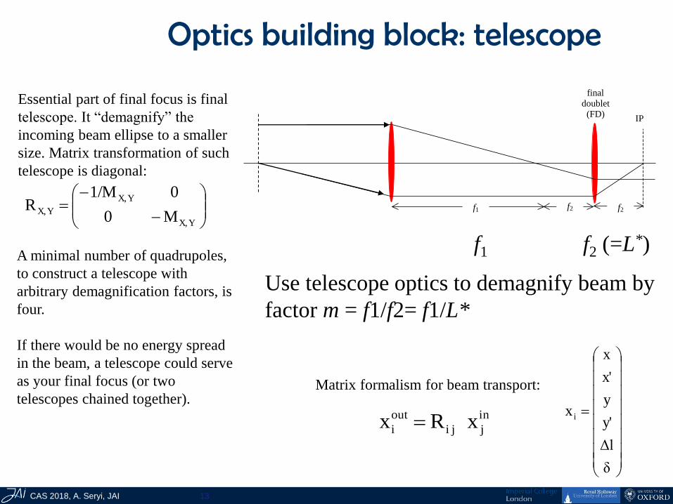
Optics building block: telescope

Use telescope optics to demagnify beam by

factor m = f1/f2= f1/L*

Essential part of final focus is final

telescope. It “demagnify” the

incoming beam ellipse to a smaller

size. Matrix transformation of such

telescope is diagonal:

YX,

YX,

YX,M0

01/MR

A minimal number of quadrupoles,

to construct a telescope with

arbitrary demagnification factors, is

four.

If there would be no energy spread

in the beam, a telescope could serve

as your final focus (or two

telescopes chained together).

δ

Δl

y'

y

x'

x

x iin

jji

out

i xRx

Matrix formalism for beam transport:


Why nonlinear elements• As sun light contains different colors, electron beam has

energy spread and get dispersed and distorted => chromatic aberrations

• For light, one uses lenses made from different materials to compensate chromatic aberrations

• Chromatic compensation for particle beams is done with nonlinear magnets– Problem: Nonlinear elements create

geometric aberrations

• The task of Final Focus system (FF) is to focus the beam to required size and compensate aberrations


How to focus to a smallest size and how big is chromaticity in FF?

• The final lens need to be the strongest• ( two lenses for both x and y => “Final Doublet” or FD )

• FD determines chromaticity of FF • Chromatic dilution of the beam

size is D/ ~ E L*/b*

• For typical parameters, D/ ~ 15-500 too big !• => Chromaticity of FF need to be compensated

E -- energy spread in the beam ~ 0.002-0.01L* -- distance from FD to IP ~ 3 - 5 mb* -- beta function in IP ~ 0.4 - 0.1 mm

Typical:

Size: (e b)1/2

Angles: (e/b)1/2

L*IP

Size at IP:

L* (e/b)1/2

+ (e b)1/2 E

Beta at IP:L* (e/b)1/2 = (e b* )1/2

=> b* = L*2/b

Chromatic dilution: (e b)1/2 E / (e b* )1/2

= E L*/b*


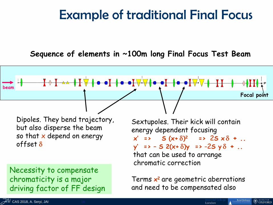
Sequence of elements in ~100m long Final Focus Test Beam

beam

Focal point

Dipoles. They bend trajectory,but also disperse the beamso that x depend on energy offset d

Sextupoles. Their kick will containenergy dependent focusingx’ => S (x+ d)2 => 2S x d + ..y’ => – S 2(x+ d)y => -2S y d + ..that can be used to arrangechromatic correction

Terms x2 are geometric aberrationsand need to be compensated also

Necessity to compensate chromaticity is a major driving factor of FF design

Example of traditional Final Focus


Final Focus Test Beam –optics with traditional non-local chromaticity compensation

Achieved (in ~1990s) ~70nm vertical beam size


Synchrotron Radiation in FF magnets

Energy spread caused by SR in bends and quads is also a major driving factor of FF design

• Bends are needed for compensation of chromaticity

• SR causes increase of energy spread which may perturb compensation of chromaticity

• Bends need to be long and weak, especially at high energy

• SR in FD quads is also harmful (Oide effect) and may limit the achievable beam size

Field lines

Field left behind


Synchrotron radiation

on-the-back-of-the envelope – power loss

dVEW 2

Energy in the field left behind (radiated !):

The field the volume2r

eΕ dSrV 2

2

2

2

22 rr

erE

dS

dW

Energy loss per unit length:

Compare with

exact formula:2

42

R

γe

3

2

dS

dW

Substitute and get an estimate:22γ

Rr

2

42

R

γe

dS

dW

22γ

R1

v

cRr

R + rR

Field left behind

Field lines

Gaussian units on this page!

r

rr


Estimation of characteristic frequency of SR photons

During what time Dt the observer will see the photons?

Observer

1/γ

2

v = c

RPhotons emitted during travel

along the 2R/ arc will be observed.

For >>1 the emitted photons

goes into 1/ cone.

c

v1

γ

2RdS

Photons travel with speed c, while particles with v.

At point B, separation between photons and particles is

A B

Therefore, observer will see photons during 3γc

Rβ1

γc

2R

c

dSΔt

R

γc

2

3ω

3

c Compare with exact formula:Estimation of characteristic frequencyR

γc

Δt

1ω

3

c


Estimation of energy spread growth due to SR

We estimated the rate of energy loss : And the characteristic frequencyR

γcω

3

c 2

42

R

γe

dS

dW

The photon energy 2

e

33

cc mcλR

γ

R

cγωε

2

2

emc

er

c

eα

2

α

rλ e

e where

Compare with exact formula:

3

5

ee

2

R

γλr

324

55

dS

ΔE/Ed

Number of photons emitted per unit length R

γ

dS

dW1

dS

dN

e

c

(per angle q : )θγαN

3

5

ee

2

R

γλr

dS

ΔE/EdWhich gives:

The energy spread DE/E will grow due to statistical fluctuations ( ) of the number of emitted photons :

22

2

c

2

γmc

1

dS

dNε

dS

ΔE/Ed

N


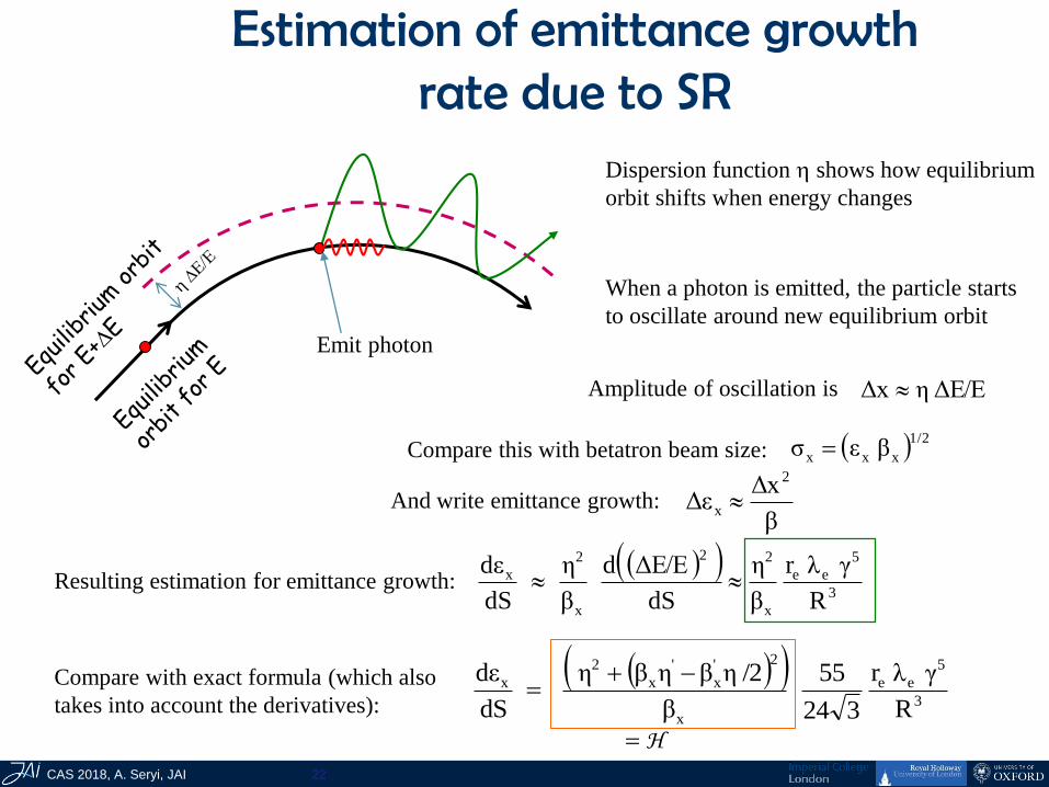
Estimation of emittance growth rate due to SR

Dispersion function shows how equilibrium

orbit shifts when energy changes

When a photon is emitted, the particle starts

to oscillate around new equilibrium orbit

Emit photon

ΔE/EηΔx Amplitude of oscillation is

1/2

xxx βεσ Compare this with betatron beam size:

And write emittance growth: β

Δx Δε

2

x

Resulting estimation for emittance growth:

3

5

ee

x

22

x

2

x

R

γλr

β

η

dS

ΔE/Ed

β

η

dS

dε

Compare with exact formula (which also

takes into account the derivatives):

3

5

ee

x

2'

x

'

x

2

x

R

γλr

324

55

β

/2ηβηβη

dS

dε

H


Let’s apply SR formulae to estimate Oide effect (SR in FD)

Final quad

** ε/βθ

** β εσ

IP divergence:

IP size:

R

L L*

*θ / L R Radius of curvature of the trajectory:

Energy spread obtained in the quad:

3

5

ee

2

R

Lγλr

E

ΔE

Growth of the IP beam size: 2

2**2

0

2

E

ΔEθLσσ

This achieve minimum possible value:

5/71/7

ee

2/7*

1/7

1min γελrL

LC35.1σ

When beta* is:

3/72/7

ee

4/7*

2/7

1optimal γεγλrL

LC29.1β

5/2

*

5

ee

2*

1

*2

β

εγλr

L

LCβεσ

Which gives ( where C1 is ~ 7 (depend on FD params.))

Note that beam distribution at IP will be non-Gaussian. Usually need to use tracking to estimate impact on

luminosity. Note also that optimal b may be smaller than the z (i.e cannot be used).


TeV FF with non-local chromaticity

compensation

0 200 400 600 800 1000 1200 1400 1600 18000

100

200

300

400

500

b1 / 2 (

m1 / 2 )

s (m)

-0.15

-0.10

-0.05

0.00

0.05

0.10

0.15

y

x

by

1/2

bx

1/2

(m

)

Traditional FF(NLC FF, circa 1999)L*=2m, TeV energy reach

• Chromaticity is compensated by sextupoles in dedicated sections

• Geometrical aberrations are canceled by using sextupoles in pairs with M= -I

Final

DoubletX-Sextupoles Y-Sextupoles

Problems:

• Chromaticity not locally compensated– Compensation of aberrations is not

ideal since M ≠ -I for off energy particles

– Large aberrations for beam tails

Chromaticity arise at FD but pre-compensated 1000m upstream


FF with local chromatic correction

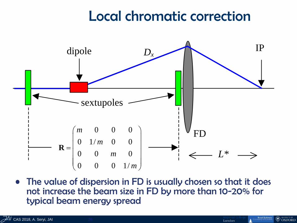
• Chromaticity is cancelled locally by two sextupoles interleaved with FD, a bend upstream generates dispersion across FD

• 2nd order dispersion produced in FD is cancelled locally provided that half of horizontal chromaticity arrive from upstream

• Geometric aberrations of the FD sextupoles are cancelled by two more sextupoles placed in phase with them and upstream of the bend

• Higher order aberrations are cancelled by optimizing transport matrices between sextupoles

P.Raimondi, A.Seryi, PRL, 86, 3779 (2001)


Local chromatic correction

• The value of dispersion in FD is usually chosen so that it does not increase the beam size in FD by more than 10-20% for typical beam energy spread

IP

FD

Dx

sextupoles

dipole

0 0 0

0 1/ 0 0

0 0 0

0 0 0 1/

m

m

m

m

R

L*


Chromatic correction in FD

x + d

IP

quadsextup.

KS KF

Quad: )ηδδx(Kηδ)(xδ)(1

Kx' 2

FF

D

)2

ηδxδ(ηKηδ)(x

2

K x'

2

S2S DSextupole:

• Straightforward in Y plane• a bit tricky in X plane:

Second order

dispersionchromaticity

If we require KS = KF to

cancel FD chromaticity, then

half of the second order

dispersion remains.

Solution:

The b-matching section

produces as much X

chromaticity as the FD, so the X

sextupoles run twice stronger

and cancel the second order

dispersion as well.

η

K2KKK

)2

ηδδx(K2x

δ)(1

Kηδ)(x

δ)(1

Kx'

FSFmatch-

2

F

match-F

D

b

b


Compare FF designs

Traditional FF, L* =2m

New FF, L* =2m

new FF

FF with local chromaticity compensation with the same

performance can be

~300m long, i.e. 6 times shorter

Moreover, its necessary length scales only as E2/5 with

energy! One can design multi-TeV FF in under a km!


IP bandwidth

Bandwidth of FF with local chromaticity correction can be better than for system with non-local correction


Aberrations & halo generation in FF

-100 -80 -60 -40 -20 0 20 40 60 80 100-100

-80

-60

-40

-20

0

20

40

60

80

100

Traditional FF New FF

Y (

mm

)X (mm)

Halo beam at the FD entrance.

Incoming beam is ~ 100 times larger than

nominal beam

• FF with non-local chr. corr. generate beam tails due to aberrations and it does not preserve betatron phase of halo particles

• FF with local chr. corr. has much less aberrations and it does not mix phases particles

Incoming beam

halo

Beam at FD

non-local chr.corr. FF

local chr.corr. FF


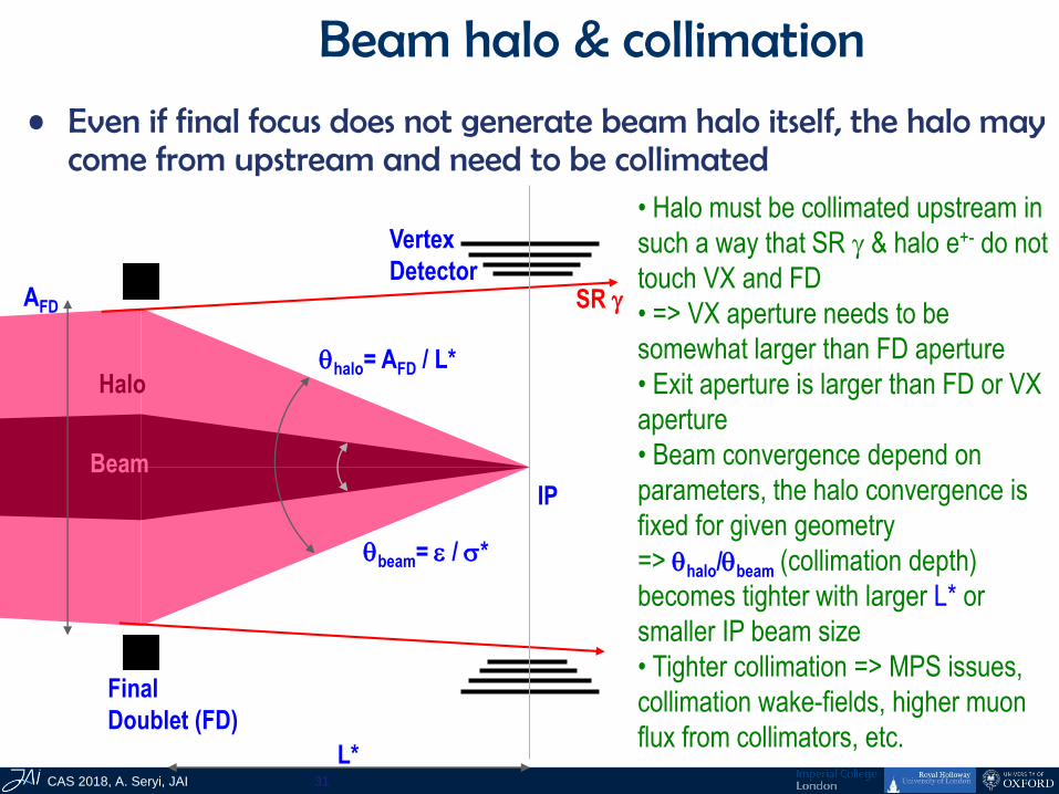
Beam halo & collimation

• Halo must be collimated upstream in

such a way that SR & halo e+- do not

touch VX and FD

• => VX aperture needs to be

somewhat larger than FD aperture

• Exit aperture is larger than FD or VX

aperture

• Beam convergence depend on

parameters, the halo convergence is

fixed for given geometry

=> qhalo/qbeam (collimation depth)

becomes tighter with larger L* or

smaller IP beam size

• Tighter collimation => MPS issues,

collimation wake-fields, higher muon

flux from collimators, etc.

Vertex

Detector

Final

Doublet (FD)

L*

IP

SR

Beam

Halo

qbeam= e / *

qhalo= AFD / L*

AFD

• Even if final focus does not generate beam halo itself, the halo may come from upstream and need to be collimated


More details on collimation

• Collimators has to be placed far from IP, to minimize background

• Ratio of beam/halo size at FD and collimator (placed in “FD phase”) remains

• Collimation depth (esp. in x) can be only ~10 or even less

• It is not unlikely that not only halo (1e-3 – 1e-6 of the beam) but full errant bunch(s) would hit the collimator

collimator


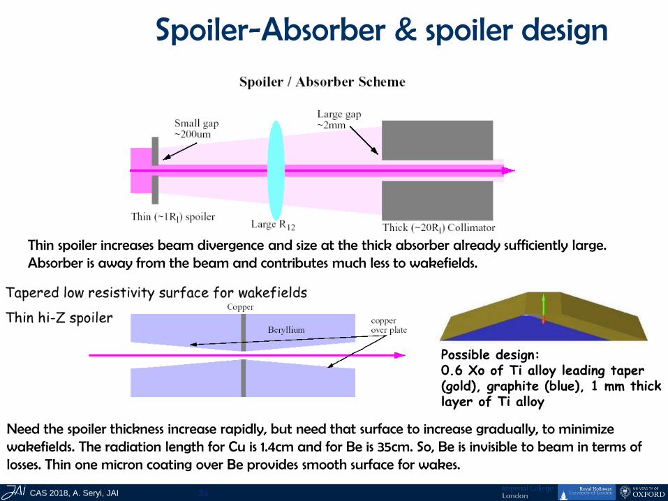
Spoiler-Absorber & spoiler design

Thin spoiler increases beam divergence and size at the thick absorber already sufficiently large. Absorber is away from the beam and contributes much less to wakefields.

Need the spoiler thickness increase rapidly, but need that surface to increase gradually, to minimize wakefields. The radiation length for Cu is 1.4cm and for Be is 35cm. So, Be is invisible to beam in terms of losses. Thin one micron coating over Be provides smooth surface for wakes.

Possible design:0.6 Xo of Ti alloy leading taper (gold), graphite (blue), 1 mm thick layer of Ti alloy


FF and Collimation

• Beam Delivery System Optics, a version with consumable spoilers

• Location of spoiler and absorbers is shown

• Collimators were placed both at FD betatron phase and at IP phase

• Two spoilers per FD and IP phase

• Energy collimator is placed in the region with large dispersion

• Secondary clean-upcollimators located in FF part

• Tail folding octupoles(see below) are included

betatron

energy


ILC FF & Collimation

• Betatron spoilers survive up to two bunches

• E-spoiler survive several bunches

• One spoiler per FD or IP phase

betatron

spoilers

E- spoiler

• Beam Delivery System Optics, a version with survivable spoilers


polarimeterskew correction /

emittance diagnostic

MPS

coll

betatron

collimation

fast

sweepers

tuneup

dump

septa

fast

kickers

energy

collimation

beta

match

energy

spectrometer

final

transformer

final

doublet

IP

energy

spectrometer

polarimeter

fast

sweepers

primary

dump


Nonlinear handling of beam tails in ILC BDS

• Can we ameliorate the incoming beam tails to relax the required collimation depth?

• One wants to focus beam tails but not to change the core of the beam– use nonlinear elements

• Several nonlinear elements needs to be combined to provide focusing in all directions– (analogy with strong focusing by FODO)

• Octupole Doublets (OD) can be used for nonlinear tail folding in ILC FF

Single octupole focus in planes and defocus on diagonals.

An octupole doublet can focus in all directions !


Strong focusing by octupoles

Effect of octupole doublet (Oc,Drift,-Oc) on

parallel beam, DQ(x,y).

• Two octupoles of different sign separated by drift provide focusing in all directions for parallel beam:

Next nonlinear term

focusing – defocusing

depends on j

Focusing in

all directions

*3423333 1 jjj q iii eLrerer D

jj q 527352 33 ii eLrer D

jireiyx

• For this to work, the beam should have small angles,

i.e. it should be parallel or diverging


Tail folding in ILC FF

Tail folding by means of two octupole doublets in the ILC final focus

Input beam has (x,x’,y,y’) = (14mm,1.2mrad,0.63mm,5.2mrad) in IP units

(flat distribution, half width) and 2% energy spread,

that corresponds approximately to N=(65,65,230,230) sigmas

with respect to the nominal beam

QF1

QD0QD6

Oct.

• Two octupole doublets give tail folding by ~ 4 times in terms of beam size in FD

• This can lead to relaxing collimation requirements by ~ a factor of 4


Tail folding or Origami Zoo

QD6

Oct.

QF5B

QD2

QD2

QF5B

QD6QF1

QD0

IP

QF1

QD0

IP


Halo collimation

Assuming 0.001 halo, beam losses along the beamline behave nicely, and SR photon losses occur only on dedicated masks

Smallest gaps are +-0.6mm with tail folding Octupoles and +-0.2mm without them.

Assumed halo sizes. Halo

population is 0.001 of the

main beam.


Dealing with muons in BDS

Long magnetized steel walls are needed to spray the muons out of the tunnel

Magnetized muon wall

2.25m

• Muons are produced during collimation

• Muon walls, installed ~300m from IP, reduce muon background in the detectors


BDS design methods & examples

Example BDS optics;design history; locationof design knobs


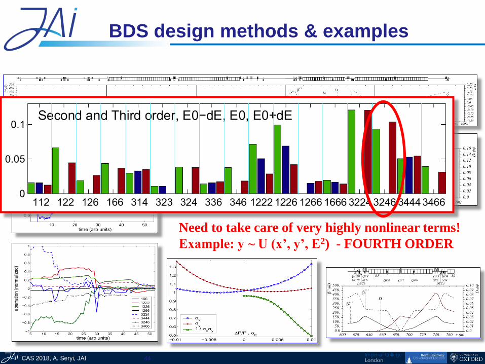
BDS design methods & examples

Need to take care of very highly nonlinear terms!

Example: y ~ U (x’, y’, E2) - FOURTH ORDER


In a practical situation …

• While designing the FF, one has a total control

• When the system is built => limited number of observable parameters (measured orbit position, beam size measured in several locations)

• The system, however, may initially have errors (errors of strength of the elements, transverse misalignments) and initial aberrations may be large

• Tuning of FF is done by optimization of “knobs” (strength, position of group of elements) chosen to affect some particular aberrations

• Experience in SLC FF and FFTB, and simulations with new FF give confidence that this is possible

Laser wire will be a tool for tuning and diagnostic of FF

Laser wire at ATF


Sextupole knobs for BDS tuning

Second ordereffect:

x’ = x’ + S (x2-y2)y’ = y’ – S 2xy

10

01R YX,

• Combining offsets of sextupoles (symmetrical or anti-symmetrical in X or Y), one can produce the following corrections at the IP – waist shift

– coupling

– dispersion

IP

To create these knobs, sextupole placed on movers


IR coupling compensation

When detector solenoid overlaps

QD0, coupling between y & x’ and y

& E causes large (30 – 190 times)

increase of IP size (green=detector

solenoid OFF, red=ON)

Even though traditional use of skew

quads could reduce the effect, the

local compensation of the fringe field

(with a little skew tuning) is the most

efficient way to ensure correction over

wide range of beam energies

without compensation

y/ y(0)=32

with compensation by

antisolenoid

y/ y(0)<1.01

QD0

antisolenoid

SD0

Y. Nosochkov, A. Seryi, Phys.Rev.ST Accel.Beams 8:021001, 2005


Detector Integrated Dipole• With a crossing angle, when beams cross solenoid field, vertical orbit arise

• For e+e- the orbit is anti-symmetrical and beams still collide head-on

• If the vertical angle is undesirable (to preserve spin orientation or the e-e-luminosity), it can be compensated locally with DID

• Alternatively, negative polarity of DID may be useful to reduce angular spread of beam-beam pairs (anti-DID)


Use of DID or anti-DID

Orbit in 5T SiD

SiD IP angle

zeroed

w.DID

DID field shape and scheme DID case

• The negative polarity of DID is also possible (called anti-DID)

•In this case the vertical angle at the IP is somewhat increased, but the background conditions due to low energy pairs (see below) and are improved

B. Parker, A. Seryi Phys. Rev. ST Accel. Beams 8, 041001, 2005


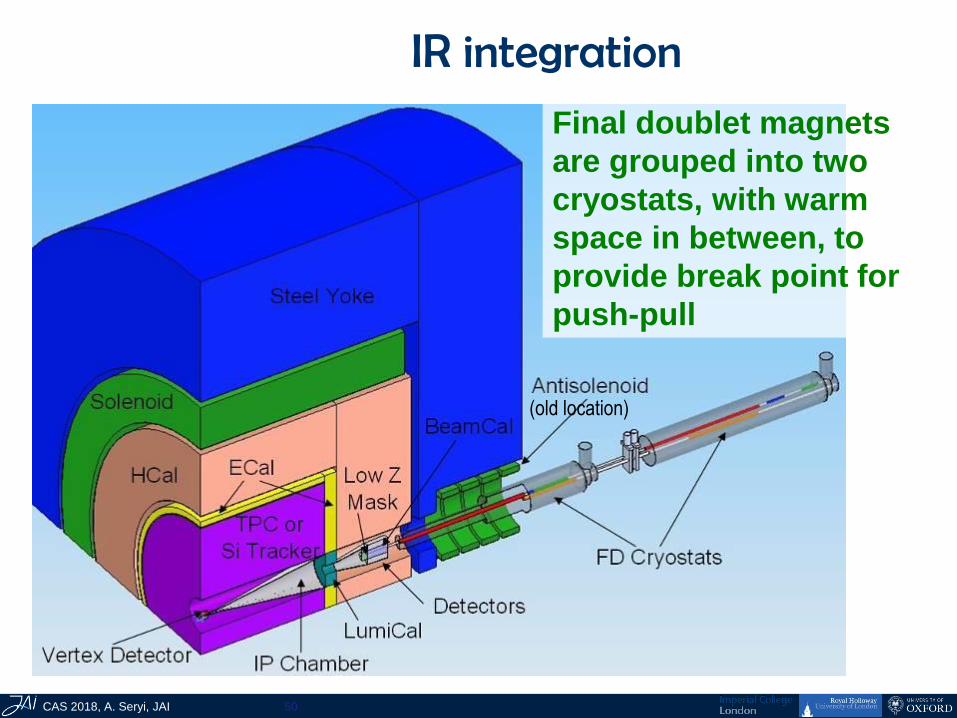
IR integration

(old location)

Final doublet magnets

are grouped into two

cryostats, with warm

space in between, to

provide break point for

push-pull


14 mrad IR


• Interaction region uses compact self-shielding SC magnets

• Independent adjustment of in- & out-going beamlines

• Force-neutral anti-solenoid for local coupling correction

Shield ON Shield OFFIntensity of color represents value of magnetic field.

to be prototyped

during EDR

new force neutral antisolenoid

Actively

shielded QD0

BNL


cancellation of the external field with a shield coil has been

successfully demonstrated at BNL

BNL prototype of self shielded quad

prototype of sextupole-octupole magnet

Coil integrated quench heater

IR magnets prototypes at

BNL

winding process


• Detailed engineering design of IR magnets and their integrationService

cryostat & cryo

connections

BNL


x

x

RF kick

Crab crossingWith crossing angle qc, the

projected x-size is

(x2+qc

2z2)0.5 ~qcz ~ 4mm

several time reduction in L

without corrections

Use transverse (crab) RF

cavity to ‘tilt’ the bunch at IP


1TeV

Beam Delivered…

e-e+ e- e-e+e+

Beam-beam effectsBeam-beam effects are not discussed in this lecture in detail as I assume you had a dedicated lecture on that


Incoherent* production of pairs• Beamstrahling photons, particles

of beams or virtual photons interact, and create e+e- pairs

Breit-Wheeler process e+e-

Bethe-Heitler processe ee+e-

Landau-Lifshitz processee eee+e-

*) Coherent pairs are generatedby photon in the field of opposite bunch. It is negligible for ILC parameters.


Deflection of pairs by beam

• Pairs are affected by the beam (focused or defocused)

• Deflection angle and Ptcorrelate

• Max angle estimated as (where is fractional energy):

• Bethe-Heitler pairs have hard edge, Landau-Lifshitzpairs are outside


Deflection of pairs by detector solenoid

• Pairs are curled by the solenoid field of detector

• Geometry of vertex detector and vacuum chamber chosen in such a way that most of pairs (B-H) do not hit the apertures

• Only small number (L-L) of pairs would hit the VX apertures

Z(cm)


Use of anti-DID to direct pairs

anti-DID case

Anti-DID field can be used to direct most of pairs into extraction hole and thus improve somewhat the background conditions

Pairs in IR region


Beam Delivery & MDI elements

14mr IR

Final FocusE-spectrometer

polarimeter

Diagnostics

Tune-up dump

Beam

Switch

Yard

Sacrificial

collimators

Extraction with

downstream diagnostics

grid: 100m*1m

Main dump

Muon wall

Tune-up & emergency

Extraction

IR Integration

Final Doublet

1TeV CM, single IR, two detectors, push-pull

Collimation: b, E

• Very forward region

•Beam-CAL

•Lumi-Cal

•Vertex


BDS functions and optics

IPlinac


Optics for outgoing beam

Extraction optics need to handle the beam with ~60% energy

spread, and provides energy and polarization diagnostics

100

GeV

250

GeV

“low P”

“nominal”

Beam spectra

Pola

rim

ete

r

E-s

pectr

om

ete

r


Beam dump

• 17MW power (for 1TeV CM)

• Rastering of the beam on 30cm double window

• 6.5m water vessel; ~1m/s flow

• 10atm pressure to prevent boiling

• Three loop water system

• Catalytic H2-O2 recombiner

• Filters for 7Be

• Shielding 0.5m Fe & 1.5m concrete


ATF and ATF2


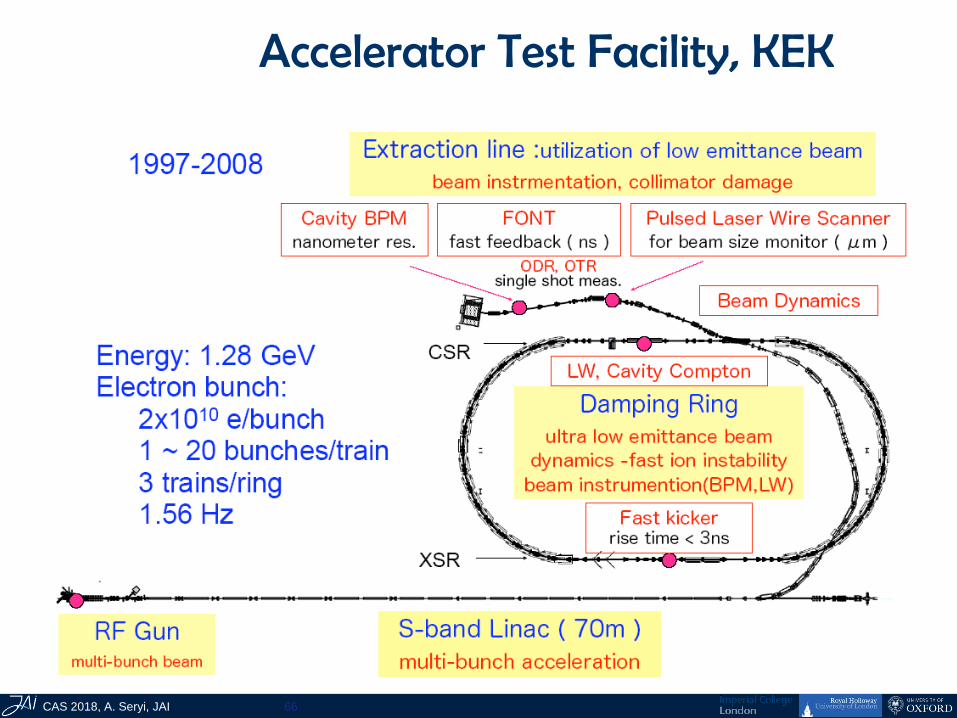
Accelerator Test Facility, KEK


ATF2

Scaled ILC final focus

ATF2: model of ILC beam deliverygoals: ~37nm beam size; nm level beam stability

• Dec 2008: first pilot run; Jan 2009: hardware commissioning• Feb-Apr 2009: large b; BSM laser wire mode; tuning tools commissioning• Oct-Dec 2009: commission interferometer mode of BSM & other hardware


ATF2 & ILC parameters

Parameters ATF2 ILC

Beam Energy, GeV 1.3 250

L*, m 1 3.5-4.2

ex/y, m*rad 3E-6 / 3E-8 1E-5 / 4E-8

IP bx/y, mm 4 / 0.1 21 / 0.4

IP ’, rad 0.14 0.094

E, % ~0.1 ~0.1

Chromaticity ~1E4 ~1E4

nbunches 1-3 (goal A) ~3000

nbunches 3-30 (goal B) ~3000

Nbunch 1-2E10 2E10

IP y, nm 37 5


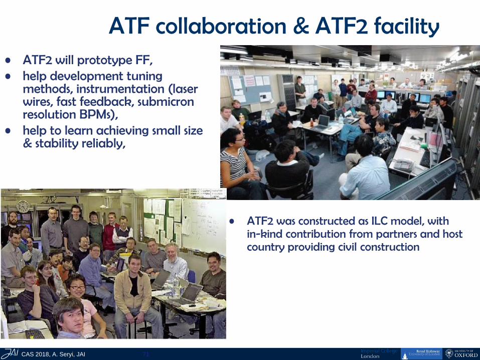
ATF collaboration & ATF2 facility• ATF2 will prototype FF,• help development tuning

methods, instrumentation (laser wires, fast feedback, submicron resolution BPMs),

• help to learn achieving small size & stability reliably,

• ATF2 was constructed as ILC model, with in-kind contribution from partners and host country providing civil construction


ATF International organization is defined by MOU signed by 25 institutions:

http://atf.kek.jp/

MOU: Mission of ATF/ATF2 is three-fold: • ATF, to establish the technologies associated with producing the electron beams with the quality required for ILC and provide such beams to ATF2 in a stable and reliable manner.• ATF2, to use the beams extracted from ATF at a test final focus beamline which is similar to what is envisaged at ILC. The goal is to demonstrate the beam focusing technologies that are consistent with ILC requirements. For this purpose, ATF2 aims to focus the beam down to a few tens of nm (rms) with a beam centroid stability within a few nm for a prolonged period of time.• Both the ATF and ATF2, to serve the mission of providing the young scientists and engineers with training opportunities of participating in R&D programs for advanced accelerator technologies.

http://atf.kek.jp/


QD0 QF1SD0 SF1

ATF2 final doublet

ILC Final Doubletlayout


Advanced beam instrumentation at ATF2

• BSM to confirm 35nm beam size• nano-BPM at IP to see the nm stability• Laser-wire to tune the beam• Cavity BPMs to measure the orbit• Movers, active stabilization, alignment system• Intratrain feedback, Kickers to produce ILC-like train

IP Beam-size monitor (BSM)

(Tokyo U./KEK, SLAC, UK)

Laser-wire beam-size

Monitor (UK group)

Cavity BPMs, for use with Q

magnets with 100nm

resolution (PAL, SLAC, KEK)

Cavity BPMs with

2nm resolution,

for use at the IP

(KEK)

Laser wire at ATF


IP Beam Size monitor

Jul 2005: BSM after it arrived to Univ. of Tokyo

FFTB sample : y = 70 nm

Shintake monitor schematics

• BSM:– refurbished & much

improved FFTB Shintake BSM

– 1064nm=>532nm


Nanobeams at ATF2 Final Focus

Beam Size 44 nm observed*,(Goal (ideal size): 37 nm

corresponding to 6 nm at ILC)

0

50

100

150

200

250

300

350

400

Mea

sured

Min

imu

m

Beam

Siz

e (

nm

)

Dec 2010

Dec 2012

Feb-Jun 2012

Mar 2013Apr 2014

Eart

hq

ua

ke (

Mar

2011)

May 2014

Jun 2014

0

200

400

600

800

1000

10 20 30 40 50 60 70

2-8 deg. mode30 deg. mode174 deg. mode

y (

nm

)

Time (hours) from Operation Start after 3 days shutdown

Week from April 14, 2014

Operation of Final Focus with local chromatic correction verified successfully

It took long time as we needed to develop instrumentation and tuning procedures

*) Effects (wakefields and magnet nonlinearities) contributing to ATF2 beam size (at 1.2 GeV) would not matter at ILC energy


Some of ATF Collaboration photos


• In the previous lectures we have

discussed how to estimate effects of

dynamic misalignments on beams

• This can be done analytically, and

even taking onto account feedbacks

– E.g. one-to-one steering in linac

– Or IP feedforward

• In practice, detailed estimations are

performed by end-to-end simulations

– Or “DR=>IP<=DR” simulations

FF and stability


Ground motion models

• Based on data, build

modeling P(w,k)

spectrum

of ground motion

which includes:

– Elastic waves

– Slow ATL motion

– Systematic motion

– Cultural noises 1E-4 1E-3 0.01 0.1 1 10 100

0.1

1

10

100

"Model A"

"Model C"

"Model B"

Inte

gra

ted r

ms m

otion, nm

Frequency, Hz

Example of integrated spectra of absolute

(solid lines) and relative motion for 50m

separation obtained from the models


Ground motion induced beam offset at IP

www ddkFkGkP )()(),(rms beam offset at IP:

)(kG

)(wF

),( kP w

Spectral response

function

- 2D spectrum of ground motion

Performance of inter-

bunch feedback

1 -11

-1

2

-2

2

-2

3

-3

-3

0

-4

0

0

-5

-10

-15

-20

-25

-30

-35

log(P)

a)

Ch

ara

cte

ris

tic

of

Fe

ed

ba

ck

~(F/F0)2

F/F0

~11

F(ω)

b)1

c)

Sp

ec

tra

l re

sp

on

se

fun

cti

on

G(k)

k(1/m)

10-3 10-2 10-1 1 10

10-3

10-2

10-1

1

10

10-6

10-5

10-4


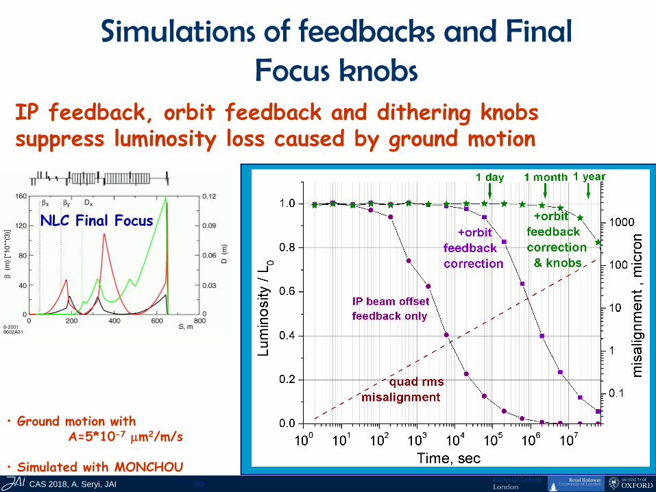
Simulations of feedbacks and Final Focus knobs

NLC Final Focus

IP feedback, orbit feedback and dithering knobs suppress luminosity loss caused by ground motion

• Ground motion with A=5*10-7 mm2/m/s

• Simulated with MONCHOU


e- source => Interaction Point <= e+ source

integrated simulations

IP

1.98GeV

250GeV1.98GeV

250GeV

500GeV CM

linac bypass bypass linac

BDS


Intermediate ground motion

nlcallgpipfb06_anm.gif


Noisy ground motion

nlcallgpipfb07_anm.gif


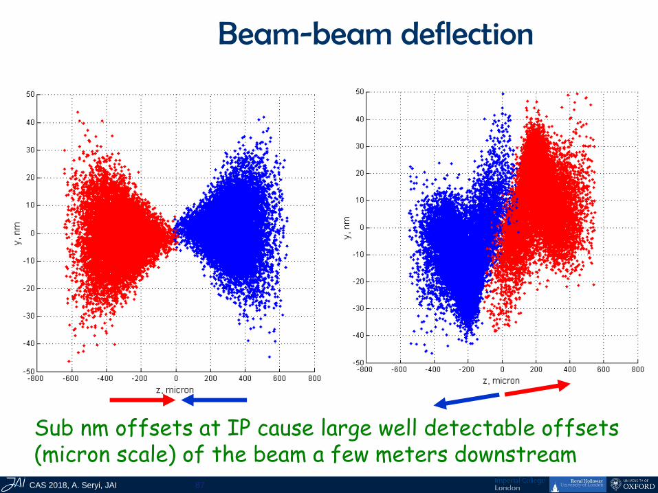
Beam-beam deflection

Sub nm offsets at IP cause large well detectable offsets (micron scale) of the beam a few meters downstream


Beam-Beam orbit feedback

Use strong beam-beam kick to keep beams colliding

Shorten BPM-Kicker path for NLC or CLIC design


Beam offset at the IP of NLC FF for different GM models

Characteristic of Feedback

1

~ 1

~ (F/F0)2

F/F0

1E-3 0.01 0.1 1 10

1E-6

1E-5

1E-4

1E-3

0.01

0.1

1

10

Gy

OFFSET for NLC FFS

Spectr

al re

sponse function

k (1/m)

www ddkFkGkP )()(),(rms beam offset at IP:


Beam-Beam orbit feedback

IP

BPM

qbb

FDBK

kicker

Dy

e

e

use strong beam-beam kick to keep beams colliding


ILC intratrain simulation

[Glen White]

ILC intratrain feedback (IP position and angle optimization), simulated with realistic errors in the linac and “banana” bunches.


• To finish up, lets discuss what FF design

approaches that we discussed apply to circular

colliders

• Circular e+e- colliders – a lot in common:

– Design challenges (chromaticity) similar to linear

collider – similar design of FF

– Non-local chromaticity compensation

– Local chromaticity compensation

• Note possible confusion of terminology:

(in circular colliders sometime non-local means chromatic

compensation by sextupoles in arcs, while local means by

sextupoles in cc sections of FF, but not in final doublet)

• Circular hh – not a lot in common

FF for circular colliders


SuperKEKB FF is designed as classic FF with non-local chromaticity compensation

This version is more suitable for circular colliders, due to dynamic aperture performance

It has been discussed to test CLIC non-local chr comp FF version at SuperKEKB, P. Thrane et al, LCSW 2017

B-Factory SuperKEKB


Comparisons of FF


SuperB


FCC-e+e-


FCC-hh Parameters

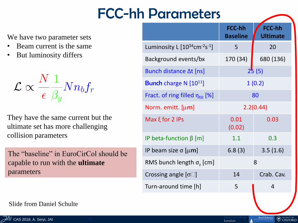
We have two parameter sets

• Beam current is the same

• But luminosity differs

They have the same current but the

ultimate set has more challenging

collision parameters

The “baseline” in EuroCirCol should be

capable to run with the ultimate

parameters

Slide from Daniel Schulte

FCC-hhBaseline

FCC-hhUltimate

Luminosity L [1034cm-2s-1] 5 20

Background events/bx 170 (34) 680 (136)

Bunch distance Δt [ns] 25 (5)

Bunch charge N [1011] 1 (0.2)

Fract. of ring filled ηfill [%] 80

Norm. emitt. [mm] 2.2(0.44)

Max ξ for 2 IPs 0.01(0.02)

0.03

IP beta-function β [m] 1.1 0.3

IP beam size σ [mm] 6.8 (3) 3.5 (1.6)

RMS bunch length σz [cm] 8

Crossing angle [] 14 Crab. Cav.

Turn-around time [h] 5 4


The FCC-hh, housed in a

97.75 km perimeter

racetrack tunnel filled

with 16 T SC magnets,

includes four EIRs -- two

for nominal/high

luminosity and two for

low-luminosity

experiments

Each of the EIR straight

sections is 1400 m long,

while in low-luminosity

EIR sections the

experiments are

combined with injection

sections

FCC-hh


• FF needs to reach b* around 0.1 m

• From chromatic properties this is not a

large challenge

• There is no need for dedicated chromatic

correction sections

• Challenges come from other places:

• Dynamic aperture

• The need to provide shielding of triplets

from collision debris – 15-50mm of

shielding may be needed

• The need to provide good stay-clear for

beam tails

FCC-hh

IP

Q1 Q2 Q3L*

45m 7m 2m

15

44.2

15

33.2 24.2

Length (m)

106 111 97Gradient (T/m)

Coil Radius (mm)

Shielding (mm)

Aperture Ø (mm) 86 108 126

98.3 98.3 98.3

15Main EIR inner triplet – inner coil radius, clear aperture, gradient, thickness of shielding and length of individual quadrupole

Example of FCC-hh

FF triplet layout


FCC-hh triplet FF and Beam Stay Clear

• Triplet aperture still allows for b* below 0.1m at beam stay clear of 15.5 and

with 15mm thick shielding inside quadrupole apertures

• Alternative option with thick shielding of 48mm still allows to reach b* = 0.2m


FCC-hh FF triplet and shielding

Q1

106 T/mQ2

111 T/mQ3

97 T/m

Abs:4.4 cm Abs:3.3 cm Abs: 2.4cm


• Thank you for your attention!

final focus layouts and stability considerations · cas 2018, a. seryi, jai 2 we will focus here on...

Documents