final florida greenhouse gas inventory and reference case
TRANSCRIPT
Final Florida Greenhouse Gas Inventory and
Reference Case Projections 1990-2025
Center for Climate Strategies October 2008
Principal Authors: Randy Strait, Maureen Mullen, Bill Dougherty, Andy Bollman, Rachel Anderson, Holly Lindquist, Luana Williams, Manish Salhotra, Jackson Schreiber

FINAL Florida GHG Inventory and Reference Case Projection ©CCS, October 2008
[This page intentionally left blank.]
FINAL Florida GHG Inventory and Reference Case Projection ©CCS, October 2008
Florida Department of Environmental Protection i Center for Climate Strategies www.dep.state.fl.us www.climatestrategies.us
Executive Summary The Center for Climate Strategies (CCS) prepared this report for the Florida Department of Environmental Protection (DEP) as part of the Governor’s Action Team on Energy and Climate Change process. This report presents an assessment of the State’s greenhouse gas (GHG) emissions and anthropogenic sinks (carbon storage) from 1990 to 2025. The preliminary draft report documenting the GHG emissions inventory and reference case projections, completed in June 2008, served as a starting point to assist the State, as well as the Florida Climate Action Team (CAT) and its Technical Work Groups (TWG), with an initial comprehensive understanding of Florida’s current and possible future GHG emissions. The draft report was provided to the CAT and its TWGs to inform them in the identification and analysis of policy options for mitigating GHG emissions.1 The CAT and TWGs have reviewed, discussed, and evaluated the draft GHG inventory and reference case projections and the methodologies used in developing them as well as alternative data and approaches for improving the draft GHG inventory and forecast. The inventory and forecast as well as this report have been revised to address the comments provided and approved by the CAT. Emissions and Reference Case Projections (Business-as-Usual) Florida’s anthropogenic GHG emissions and anthropogenic sinks (carbon storage) were estimated for the period from 1990 to 2025. Historical GHG emission estimates (1990 through 2005)2 were developed using a set of generally accepted principles and guidelines for State GHG emissions, relying to the extent possible on Florida-specific data and inputs where available. The reference case projections (2006-2025) are based on a compilation of various projections of electricity generation, fuel use, and other GHG-emitting activities for Florida, along with a set of simple, transparent assumptions described in the appendices of this report. The inventory and projections cover the six types of gases included in the US Greenhouse Gas Inventory: carbon dioxide (CO2), methane (CH4), nitrous oxide (N2O), hydrofluorocarbons (HFCs), perfluorocarbons (PFCs), and sulfur hexafluoride (SF6). Emissions of these GHGs are presented using a common metric, CO2 equivalence (CO2e), which indicates the relative contribution of each gas, per unit mass, to global average radiative forcing on a global warming potential- (GWP-) weighted basis.3
1 “Draft Florida Greenhouse Gas Inventory and Reference Case Projections, 1990-2025,” prepared by the Center for Climate Strategies for the Florida Department of Environmental Protection, June 2008. 2 The last year of available historical data varies by sector; ranging from 2000 to 2005. 3 Changes in the atmospheric concentrations of GHGs can alter the balance of energy transfers between the atmosphere, space, land, and the oceans. A gauge of these changes is called radiative forcing, which is a simple measure of changes in the energy available to the Earth–atmosphere system. Holding everything else constant, increases in GHG concentrations in the atmosphere will produce positive radiative forcing (i.e., a net increase in the absorption of energy by the Earth). See: Boucher, O., et al. "Radiative Forcing of Climate Change." Chapter 6 in Climate Change 2001: The Scientific Basis. Contribution of Working Group 1 of the Intergovernmental Panel on Climate Change Cambridge University Press. Cambridge, United Kingdom. Available at: http://www.grida.no/climate/ipcc_tar/wg1/212.htm.

FINAL Florida GHG Inventory and Reference Case Projection ©CCS, October 2008
Florida Department of Environmental Protection ii Center for Climate Strategies www.dep.state.fl.us www.climatestrategies.us
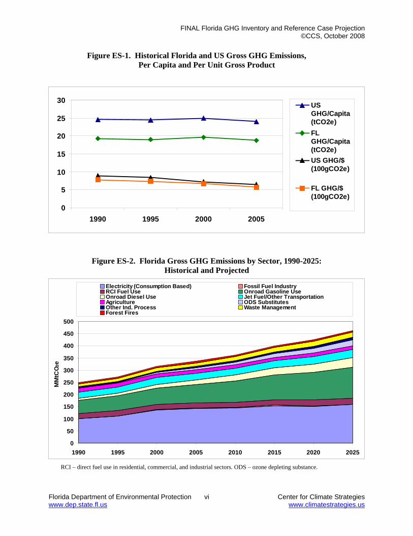
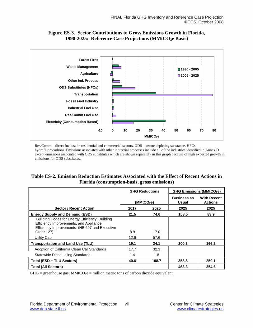
As shown in Table ES-1, activities in Florida accounted for approximately 337 million metric tons (MMt) of gross4 CO2e emissions (consumption basis) in 2005, an amount equal to about 4.7% of total US gross GHG emissions.5 Florida’s gross GHG emissions are rising faster than those of the nation as a whole (gross emissions exclude carbon sinks, such as forests). Florida’s gross GHG emissions increased by about 35% from 1990 to 2005, while national emissions rose by 16% from 1990 to 2005. The growth in Florida’s emissions from 1990 to 2005 is primarily associated with the electricity consumption and transportation sectors. Estimates of carbon sinks within Florida’s forests, including urban forests and land use changes, have also been included in this report. The current estimates indicate that about 27 MMtCO2e were stored in Florida forest biomass in 2005. This leads to net emissions of 309 MMtCO2e in Florida in 2005. Figure ES-1 illustrates the State’s emissions per capita and per unit of economic output.6 On a per capita basis, gross CO2e emissions in 1990 were about 19 metric tons (t) per capita, lower than the 1990 national average of 25 tCO2e per capita. Per capita emissions in Florida changed very little between 1990 and 2005, staying relatively constant at 19 tCO2e per capita in 2005. National per capita emissions decreased slightly to 24 MtCO2e per capita from 1990 to 2005. Like the nation as a whole, Florida’s economic growth exceeded emissions growth throughout the 1990-2005 period, leading to declining estimates of GHG emissions per unit of state product. From 1990 to 2005, emissions per unit of gross product dropped by 26%, both in Florida and nationally.7 The principal sources of Florida’s GHG emissions in 2005 are electricity consumption and transportation accounting for 42% and 36% of Florida’s gross GHG emissions in 2005, respectively. As illustrated in Figure ES-2 and shown numerically in Table ES-1, under the reference case projections, Florida’s gross GHG emissions continue to grow, and are projected to climb to about 463 MMtCO2e by 2025, reaching 86% above 1990 levels. As shown in Figure ES-3, the transportation sector is projected to be the largest contributor to future emissions growth in Florida, followed by emissions associated with the increasing use of HFCs and PFCs as substitutes for ozone-depleting substances (ODS) in refrigeration, air conditioning, and other applications and emissions from electricity consumption. The industrial processes sector is projected to have the most rapid growth between 1990 and 2025, increasing by 728% over the
4 Excluding GHG emissions removed due to forestry and other land uses and including GHG emissions associated with imported electricity. 5 The national emissions used for these comparisons are based on 2005 emissions from Inventory of US Greenhouse Gas Emissions and Sinks: 1990–2006, April 15, 2008, US EPA # 430-R-08-005, http://www.epa.gov/climatechange/emissions/usinventoryreport.html. 6 Florida population data from the Demographic Estimating Conference Database, updated August 2007. http://edr.state.fl.us/population.htm 7 Based on real gross domestic product (millions of chained 2000 dollars) that excludes the affects of inflation, available from the US Bureau of Economic Analysis (http://www.bea.gov/regional/gsp/). The national emissions used for these comparisons are based on 2005 emissions from the 2008 version of EPA’s GHG inventory report (http://www.epa.gov/climatechange/emissions/usinventoryreport.html).
FINAL Florida GHG Inventory and Reference Case Projection ©CCS, October 2008
Florida Department of Environmental Protection iii Center for Climate Strategies www.dep.state.fl.us www.climatestrategies.us
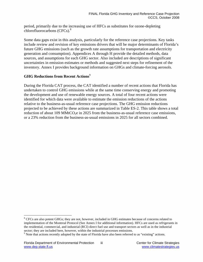
period, primarily due to the increasing use of HFCs as substitutes for ozone-depleting chlorofluorocarbons (CFCs).8 Some data gaps exist in this analysis, particularly for the reference case projections. Key tasks include review and revision of key emissions drivers that will be major determinants of Florida’s future GHG emissions (such as the growth rate assumptions for transportation and electricity generation and consumption). Appendices A through H provide the detailed methods, data sources, and assumptions for each GHG sector. Also included are descriptions of significant uncertainties in emission estimates or methods and suggested next steps for refinement of the inventory. Annex I provides background information on GHGs and climate-forcing aerosols. GHG Reductions from Recent Actions9 During the Florida CAT process, the CAT identified a number of recent actions that Florida has undertaken to control GHG emissions while at the same time conserving energy and promoting the development and use of renewable energy sources. A total of four recent actions were identified for which data were available to estimate the emission reductions of the actions relative to the business-as-usual reference case projections. The GHG emission reductions projected to be achieved by these actions are summarized in Table ES-2. This table shows a total reduction of about 109 MMtCO2e in 2025 from the business-as-usual reference case emissions, or a 23% reduction from the business-as-usual emissions in 2025 for all sectors combined.
8 CFCs are also potent GHGs; they are not, however, included in GHG estimates because of concerns related to implementation of the Montreal Protocol (See Annex I for additional information). HFCs are used as refrigerants in the residential, commercial, and industrial (RCI) direct fuel use and transport sectors as well as in the industrial sector; they are included here, however, within the industrial processes emissions. 9 Note that actions recently adopted by the state of Florida have also been referred to as “existing” actions.
FINAL Florida GHG Inventory and Reference Case Projection ©CCS, October 2008
Florida Department of Environmental Protection iv Center for Climate Strategies www.dep.state.fl.us www.climatestrategies.us
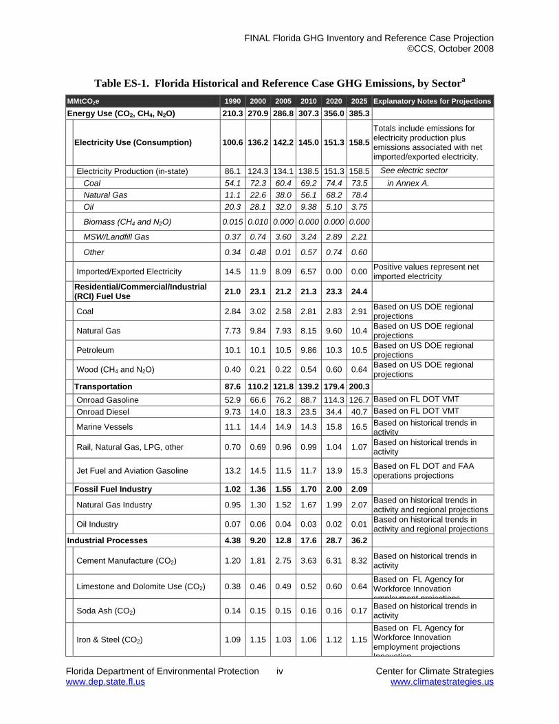
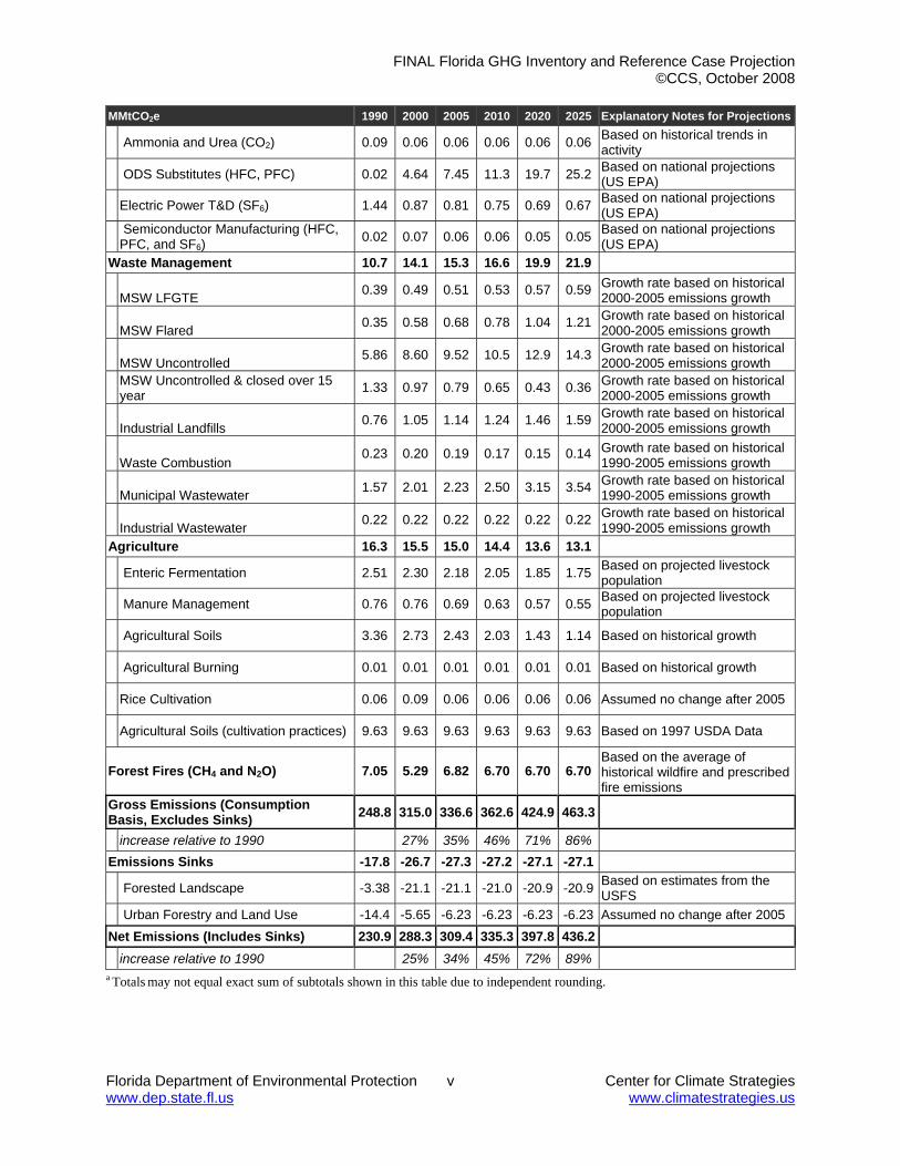
Table ES-1. Florida Historical and Reference Case GHG Emissions, by Sectora
MMtCO2e 1990 2000 2005 2010 2020 2025 Explanatory Notes for ProjectionsEnergy Use (CO2, CH4, N2O) 210.3 270.9 286.8 307.3 356.0 385.3
Electricity Use (Consumption) 100.6 136.2 142.2 145.0 151.3 158.5Totals include emissions for electricity production plus emissions associated with net imported/exported electricity.
Electricity Production (in-state) 86.1 124.3 134.1 138.5 151.3 158.5 See electric sector ti Coal 54.1 72.3 60.4 69.2 74.4 73.5 in Annex A.
Natural Gas 11.1 22.6 38.0 56.1 68.2 78.4 Oil 20.3 28.1 32.0 9.38 5.10 3.75
Biomass (CH4 and N2O) 0.015 0.010 0.000 0.000 0.000 0.000
MSW/Landfill Gas 0.37 0.74 3.60 3.24 2.89 2.21
Other 0.34 0.48 0.01 0.57 0.74 0.60
Imported/Exported Electricity 14.5 11.9 8.09 6.57 0.00 0.00 Positive values represent net imported electricity
Residential/Commercial/Industrial (RCI) Fuel Use 21.0 23.1 21.2 21.3 23.3 24.4
Coal 2.84 3.02 2.58 2.81 2.83 2.91 Based on US DOE regional projections
Natural Gas 7.73 9.84 7.93 8.15 9.60 10.4 Based on US DOE regional projections
Petroleum 10.1 10.1 10.5 9.86 10.3 10.5 Based on US DOE regional projections
Wood (CH4 and N2O) 0.40 0.21 0.22 0.54 0.60 0.64 Based on US DOE regional projections
Transportation 87.6 110.2 121.8 139.2 179.4 200.3 Onroad Gasoline 52.9 66.6 76.2 88.7 114.3 126.7 Based on FL DOT VMT
j ti Onroad Diesel 9.73 14.0 18.3 23.5 34.4 40.7 Based on FL DOT VMT j ti
Marine Vessels 11.1 14.4 14.9 14.3 15.8 16.5 Based on historical trends in activity
Rail, Natural Gas, LPG, other 0.70 0.69 0.96 0.99 1.04 1.07 Based on historical trends in activity
Jet Fuel and Aviation Gasoline 13.2 14.5 11.5 11.7 13.9 15.3 Based on FL DOT and FAA operations projections
Fossil Fuel Industry 1.02 1.36 1.55 1.70 2.00 2.09
Natural Gas Industry 0.95 1.30 1.52 1.67 1.99 2.07 Based on historical trends in activity and regional projections
Oil Industry 0.07 0.06 0.04 0.03 0.02 0.01 Based on historical trends in activity and regional projections
Industrial Processes 4.38 9.20 12.8 17.6 28.7 36.2
Cement Manufacture (CO2) 1.20 1.81 2.75 3.63 6.31 8.32 Based on historical trends in activity
Limestone and Dolomite Use (CO2) 0.38 0.46 0.49 0.52 0.60 0.64Based on FL Agency for Workforce Innovation employment projections
Soda Ash (CO2) 0.14 0.15 0.15 0.16 0.16 0.17 Based on historical trends in activity
Iron & Steel (CO2) 1.09 1.15 1.03 1.06 1.12 1.15Based on FL Agency for Workforce Innovation employment projections Innovation
FINAL Florida GHG Inventory and Reference Case Projection ©CCS, October 2008
Florida Department of Environmental Protection v Center for Climate Strategies www.dep.state.fl.us www.climatestrategies.us
MMtCO2e 1990 2000 2005 2010 2020 2025 Explanatory Notes for Projections
Ammonia and Urea (CO2) 0.09 0.06 0.06 0.06 0.06 0.06 Based on historical trends in activity
ODS Substitutes (HFC, PFC) 0.02 4.64 7.45 11.3 19.7 25.2 Based on national projections (US EPA)
Electric Power T&D (SF6) 1.44 0.87 0.81 0.75 0.69 0.67 Based on national projections (US EPA)
Semiconductor Manufacturing (HFC, PFC, and SF6)
0.02 0.07 0.06 0.06 0.05 0.05 Based on national projections (US EPA)
Waste Management 10.7 14.1 15.3 16.6 19.9 21.9
MSW LFGTE 0.39 0.49 0.51 0.53 0.57 0.59 Growth rate based on historical 2000-2005 emissions growth
MSW Flared 0.35 0.58 0.68 0.78 1.04 1.21 Growth rate based on historical 2000-2005 emissions growth
MSW Uncontrolled 5.86 8.60 9.52 10.5 12.9 14.3 Growth rate based on historical 2000-2005 emissions growth
MSW Uncontrolled & closed over 15 year 1.33 0.97 0.79 0.65 0.43 0.36 Growth rate based on historical
2000-2005 emissions growth
Industrial Landfills 0.76 1.05 1.14 1.24 1.46 1.59 Growth rate based on historical 2000-2005 emissions growth
Waste Combustion
0.23 0.20 0.19 0.17 0.15 0.14 Growth rate based on historical 1990-2005 emissions growth
Municipal Wastewater 1.57 2.01 2.23 2.50 3.15 3.54 Growth rate based on historical 1990-2005 emissions growth
Industrial Wastewater 0.22 0.22 0.22 0.22 0.22 0.22 Growth rate based on historical 1990-2005 emissions growth
Agriculture 16.3 15.5 15.0 14.4 13.6 13.1
Enteric Fermentation 2.51 2.30 2.18 2.05 1.85 1.75 Based on projected livestock population
Manure Management 0.76 0.76 0.69 0.63 0.57 0.55 Based on projected livestock population
Agricultural Soils 3.36 2.73 2.43 2.03 1.43 1.14 Based on historical growth
Agricultural Burning 0.01 0.01 0.01 0.01 0.01 0.01 Based on historical growth
Rice Cultivation 0.06 0.09 0.06 0.06 0.06 0.06 Assumed no change after 2005
Agricultural Soils (cultivation practices) 9.63 9.63 9.63 9.63 9.63 9.63 Based on 1997 USDA Data
Forest Fires (CH4 and N2O) 7.05 5.29 6.82 6.70 6.70 6.70Based on the average of historical wildfire and prescribed fire emissions
Gross Emissions (Consumption Basis, Excludes Sinks) 248.8 315.0 336.6 362.6 424.9 463.3
increase relative to 1990 27% 35% 46% 71% 86% Emissions Sinks -17.8 -26.7 -27.3 -27.2 -27.1 -27.1
Forested Landscape -3.38 -21.1 -21.1 -21.0 -20.9 -20.9 Based on estimates from the USFS
Urban Forestry and Land Use -14.4 -5.65 -6.23 -6.23 -6.23 -6.23 Assumed no change after 2005 Net Emissions (Includes Sinks) 230.9 288.3 309.4 335.3 397.8 436.2 increase relative to 1990 25% 34% 45% 72% 89% a Totals may not equal exact sum of subtotals shown in this table due to independent rounding.
FINAL Florida GHG Inventory and Reference Case Projection ©CCS, October 2008
Florida Department of Environmental Protection vi Center for Climate Strategies www.dep.state.fl.us www.climatestrategies.us
Figure ES-1. Historical Florida and US Gross GHG Emissions, Per Capita and Per Unit Gross Product
0
5
10
15
20
25
30
1990 1995 2000 2005
USGHG/Capita(tCO2e)FLGHG/Capita(tCO2e)US GHG/$(100gCO2e)
FL GHG/$(100gCO2e)
Figure ES-2. Florida Gross GHG Emissions by Sector, 1990-2025: Historical and Projected
0
50
100
150
200
250
300
350
400
450
500
1990 1995 2000 2005 2010 2015 2020 2025
MM
tCO 2
e
Electricity (Consumption Based) Fossil Fuel IndustryRCI Fuel Use Onroad Gasoline UseOnroad Diesel Use Jet Fuel/Other TransportationAgriculture ODS SubstitutesOther Ind. Process Waste ManagementForest Fires
RCI – direct fuel use in residential, commercial, and industrial sectors. ODS – ozone depleting substance.
FINAL Florida GHG Inventory and Reference Case Projection ©CCS, October 2008
Florida Department of Environmental Protection vii Center for Climate Strategies www.dep.state.fl.us www.climatestrategies.us
Figure ES-3. Sector Contributions to Gross Emissions Growth in Florida, 1990-2025: Reference Case Projections (MMtCO2e Basis)
-10 0 10 20 30 40 50 60 70 80
Electricity (Consumption Based)
Res/Comm Fuel Use
Industrial Fuel Use
Fossil Fuel Industry
Transportation
ODS Substitutes (HFCs)
Other Ind. Process
Agriculture
Waste Management
Forest Fires
MMtCO2e
1990 - 2005
2005 - 2025
Res/Comm – direct fuel use in residential and commercial sectors. ODS – ozone depleting substance. HFCs – hydrofluorocarbons. Emissions associated with other industrial processes include all of the industries identified in Annex D except emissions associated with ODS substitutes which are shown separately in this graph because of high expected growth in emissions for ODS substitutes.
Table ES-2. Emission Reduction Estimates Associated with the Effect of Recent Actions in Florida (consumption-basis, gross emissions)
Sector / Recent Action
GHG Reductions GHG Emissions (MMtCO2e)
(MMtCO2e) Business as
Usual With Recent
Actions 2017 2025 2025 2025
Energy Supply and Demand (ESD) 21.5 74.6 158.5 83.9 Building Codes for Energy Efficiency, Building Efficiency Improvements, and Appliance Efficiency Improvements (HB 697 and Executive Order 127) 8.9 17.0 Utility Cap 12.6 57.6
Transportation and Land Use (TLU) 19.1 34.1 200.3 166.2 Adoption of California Clean Car Standards 17.7 32.3 Statewide Diesel Idling Standards 1.4 1.8
Total (ESD + TLU Sectors) 40.6 108.7 358.8 250.1 Total (All Sectors) 463.3 354.6
GHG = greenhouse gas; MMtCO2e = million metric tons of carbon dioxide equivalent.
FINAL Florida GHG Inventory and Reference Case Projection ©CCS, October 2008
Florida Department of Environmental Protection viii Center for Climate Strategies www.dep.state.fl.us www.climatestrategies.us
Table of Contents
Executive Summary ......................................................................................................................... i Acronyms and Key Terms ............................................................................................................. ix Acknowledgements ...................................................................................................................... xiii Summary of Preliminary Findings .................................................................................................. 1
Introduction ............................................................................................................................. 1 Florida Greenhouse Gas Emissions: Sources and Trends .............................................................. 2 Historical Emissions ....................................................................................................................... 4
Overview ................................................................................................................................. 4 A Closer Look at the Two Major Sources: Electricity Consumption and the Transportation Sectors ..................................................................................................................................... 6
Reference Case Projections (Business as Usual) ............................................................................ 8 Approach ....................................................................................................................................... 13
General Methodology ........................................................................................................... 13 General Principles and Guidelines ........................................................................................ 14
Key Uncertainties and Next Steps ................................................................................................ 17 Annex A. Electricity Supply and Use............................................................................................. 1 Annex B. Residential, Commercial, and Industrial (RCI) Fuel Combustion ................................. 2 Annex C. Transportation Energy Use ............................................................................................ 1 Annex D. Industrial Processes ........................................................................................................ 1 Annex E. Fossil Fuel Industries ..................................................................................................... 1 Annex F. Agriculture ...................................................................................................................... 1 Annex G. Waste Management ....................................................................................................... 1 Annex H. Forestry & Land Use ..................................................................................................... 1 Annex I. Greenhouse Gases and Global Warming Potential Values: Excerpts from the Inventory
of U.S. Greenhouse Emissions and Sinks: 1990-2000 .................................................. 1
FINAL Florida GHG Inventory and Reference Case Projection ©CCS, October 2008
Florida Department of Environmental Protection ix Center for Climate Strategies www.dep.state.fl.us www.climatestrategies.us
Acronyms and Key Terms AEO2007 – EIA’s Annual Energy Outlook 2007
bbls – Barrels
Bcf – Billion Cubic Feet
BOD – Biochemical Oxygen Demand
Btu – British Thermal Unit
C – Carbon*
CaCO3 – Calcium Carbonate
CAFE – Corporate Average Fuel Economy
CAT – Florida Climate Action Team
CEC – Commission for Environmental Cooperation
CCS – Center for Climate Strategies
CFCs – Chlorofluorocarbons*
CH4 – Methane*
CO – Carbon Monoxide*
CO2 – Carbon Dioxide*
CO2e – Carbon Dioxide equivalent*
CRP – Federal Conservation Reserve Program
DEP – Florida Department of Environmental Protection
DOE – Department of Energy
DOT – Department of Transportation
EEZ – Exclusive Economic Zone
eGRID – Emissions & Generation Resource Integrated Database
EIA – US DOE Energy Information Administration
EIIP – Emission Inventory Improvement Program
ESD – Energy Supply and Demand
FAA – Federal Aviation Administration
FAPRI – Food and Agricultural Policy Research Institute
FERC – Federal Energy Regulatory Commission
FHWA – Federal Highway Administration
FIA – Forest Inventory Analysis
FRCC – Florida Reliability Coordinating Council

FINAL Florida GHG Inventory and Reference Case Projection ©CCS, October 2008
Florida Department of Environmental Protection x Center for Climate Strategies www.dep.state.fl.us www.climatestrategies.us
Gg – Gigagrams
GHG – Greenhouse Gas*
GWh – Gigawatt-hour
GWP – Global Warming Potential*
H2CO3 – Carbonic Acid
H2O – Water Vapor*
HBFCs – Hydrobromofluorocarbons*
HC – Hydrocarbon
HCFCs – Hydrochlorofluorocarbons*
HFCs – Hydrofluorocarbons*
HWP – Harvested Wood Products
IPCC – Intergovernmental Panel on Climate Change*
kg – Kilogram
km2 – Square Kilometers
kWh – Kilowatt-hour
lb – Pound
LF – Landfill
LFG – Landfill Gas
LFGTE – Landfill Gas Collection System and Landfill-Gas-to-Energy
LMOP – Landfill Methane Outreach Program
LPG – Liquefied Petroleum Gas
Mg – Megagrams
MMBtu – Million British thermal units
MMt – Million Metric tons
MMtC – Million Metric Tons of Carbon
MMtCO2e – Million Metric tons Carbon Dioxide equivalent
MSW – Municipal Solid Waste
Mt – Metric ton (equivalent to 1.102 short tons)
MWh – Megawatt-hour
N2O – Nitrous Oxide*
NASS – National Agriculture Statistical Service
NEI – National Emissions Inventory
NEMS – National Energy Modeling System
FINAL Florida GHG Inventory and Reference Case Projection ©CCS, October 2008
Florida Department of Environmental Protection xi Center for Climate Strategies www.dep.state.fl.us www.climatestrategies.us
NERC – North American Reliability Council
NF – National Forest
NH3 – Ammonia
NMVOCs – Nonmethane Volatile Organic Compound*
NO2 – Nitrogen Dioxide*
NOx – Nitrogen Oxides*
O3 – Ozone*
ODS – Ozone-Depleting Substance*
OH – Hydroxyl radical*
OPS – Office of Pipeline Safety
PFCs – Perfluorocarbons*
ppb – parts per billion
ppm – parts per million
ppt – parts per trillion
ppmv – parts per million by volume
PSC – Florida Public Service Commission
RCI – Residential, Commercial, and Industrial
SAR – Second Assessment Report*
SED – State Energy Data
SERC – Southeastern Reliability Council
SF6 – Sulfur Hexafluoride*
SIT – State Greenhouse Gas Inventory Tool
Sinks – Removals of carbon from the atmosphere, with the carbon stored in forests, soils, landfills, wood structures, or other biomass-related products.
SO2 – Sulfur Dioxide*
t – Metric ton (equivalent to 1.102 short tons)
T&D – Transmission and Distribution
TAR – Third Assessment Report*
TLU – Transportation and Land Use
TOG – Total Organic Gas
TWG – Technical Work Group
TWh – Terawatt-hour
UNFCCC – United Nations Framework Convention on Climate Change

FINAL Florida GHG Inventory and Reference Case Projection ©CCS, October 2008
Florida Department of Environmental Protection xii Center for Climate Strategies www.dep.state.fl.us www.climatestrategies.us
US – United States
US DOE – United States Department of Energy
US EPA – United States Environmental Protection Agency
USDA – United States Department of Agriculture
USFS – United States Forest Service
USGS – United States Geological Survey
VMT – Vehicle Mile Traveled
VOCs – Volatile Organic Compound*
WW – Wastewater
yr – Year
* – See Annex I for more information.

FINAL Florida GHG Inventory and Reference Case Projection ©CCS, October 2008
Florida Department of Environmental Protection xiii Center for Climate Strategies www.dep.state.fl.us www.climatestrategies.us
Acknowledgements We appreciate all of the time and assistance provided by numerous contacts throughout Florida, as well as in neighboring States, and at federal agencies. Thanks go to in particular the staff at Florida DEP and other Florida agencies for their inputs, and in particular to Steve Adams, Julie Ferris, and Yi Zhu of the Florida DEP who provided key guidance for and review of this analytical effort. Thanks also to Michael Gillenwater for directing preparation of Annex I.

FINAL Florida GHG Inventory and Reference Case Projection ©CCS, October 2008
Florida Department of Environmental Protection 1 Center for Climate Strategies www.dep.state.fl.us www.climatestrategies.us
Summary of Preliminary Findings Introduction The Center for Climate Strategies (CCS) prepared this report for the Florida Department of Environmental Protection (DEP) as part of the Governor’s Action Team on Energy and Climate Change process. This report presents an assessment of the State’s greenhouse gas (GHG) emissions and anthropogenic sinks (carbon storage) from 1990 to 2025. The preliminary draft report documenting the GHG emissions inventory and reference case projections, completed in June 2008, served as a starting point to assist the State, as well as the Florida Climate Action Team (CAT) and its Technical Work Groups (TWG), with an initial comprehensive understanding of Florida’s current and possible future GHG emissions. The draft report was provided to the CAT and its TWGs to inform them in the identification and analysis of policy options for mitigating GHG emissions.10 The CAT and TWGs have reviewed, discussed, and evaluated the draft GHG inventory and reference case projections and the methodologies used in developing them as well as alternative data and approaches for improving the draft GHG inventory and forecast. The inventory and forecast as well as this report have been revised to address the comments provided and approved by the CAT. Emissions and Reference Case Projections (Business-as-Usual) Historical GHG emission estimates (1990 through 2005)11 were developed using a set of generally accepted principles and guidelines for State GHG emissions inventories, as described in the “Approach” section below, relying to the extent possible on Florida-specific data and inputs. The initial reference case projections (2006-2025) are based on a compilation of various projections of electricity generation, fuel use, and other GHG-emitting activities for Florida, along with a set of simple, transparent assumptions described in the appendices of this report. This report covers the six gases included in the US Greenhouse Gas Inventory: carbon dioxide (CO2), methane (CH4), nitrous oxide (N2O), hydrofluorocarbons (HFCs), perfluorocarbons (PFCs), and sulfur hexafluoride (SF6). Emissions of these GHGs are presented using a common metric, CO2 equivalence (CO2e), which indicates the relative contribution of each gas, per unit mass, to global average radiative forcing on a global warming potential- (GWP-) weighted basis.12
10 “Draft Florida Greenhouse Gas Inventory and Reference Case Projections, 1990-2025,” prepared by the Center for Climate Strategies for the Florida Department of Environmental Protection, June 2008. 11 The last year of available historical data varies by sector; ranging from 2000 to 2005. 12 Changes in the atmospheric concentrations of GHGs can alter the balance of energy transfers between the atmosphere, space, land, and the oceans. A gauge of these changes is called radiative forcing, which is a simple measure of changes in the energy available to the Earth–atmosphere system (IPCC, 2001). Holding everything else constant, increases in GHG concentrations in the atmosphere will produce positive radiative forcing (i.e., a net increase in the absorption of energy by the Earth). See: Climate Change 2001: The Scientific Basis. Intergovernmental Panel on Climate Change, J.T. Houghton, Y. Ding, D.J. Griggs, M. Noguer, P.J. van der Linden, X. Dai, C.A. Johnson, and K. Maskell (eds.). Cambridge University Press. Cambridge, United Kingdom (http://www.grida.no/climate/ipcc_tar/wg1/212.htm).

FINAL Florida GHG Inventory and Reference Case Projection ©CCS, October 2008
Florida Department of Environmental Protection 2 Center for Climate Strategies www.dep.state.fl.us www.climatestrategies.us
It is important to note that these emission estimates reflect the GHG emissions associated with the electricity sources used to meet Florida’s demands, corresponding to a consumption-based approach to emissions accounting (see “Approach” section below). Another way to look at electricity emissions is to consider the GHG emissions produced by electricity generation facilities in the State. This report covers both methods of accounting for emissions, but for consistency, all total results are reported as consumption-based.
Florida Greenhouse Gas Emissions: Sources and Trends Table 1 provides a summary of GHG emissions estimated for Florida by sector for the years 1990, 2000, 2005, 2010, 2020 and 2025. Details on the methods and data sources used to construct these draft estimates are provided in the appendices to this report. In the sections below, we discuss GHG emission sources (positive, or gross, emissions) and sinks (negative emissions) separately in order to identify trends, projections, and uncertainties clearly for each. This next section of the report provides a summary of the historical emissions (1990 through 2005) followed by a summary of the reference-case projection-year emissions (2006 through 2025) and key uncertainties. We also provide an overview of the general methodology, principles, and guidelines followed for preparing the inventories. Appendices A through H provide the detailed methods, data sources, and assumptions for each GHG sector. Annex I provides background information on GHGs and climate-forcing aerosols.
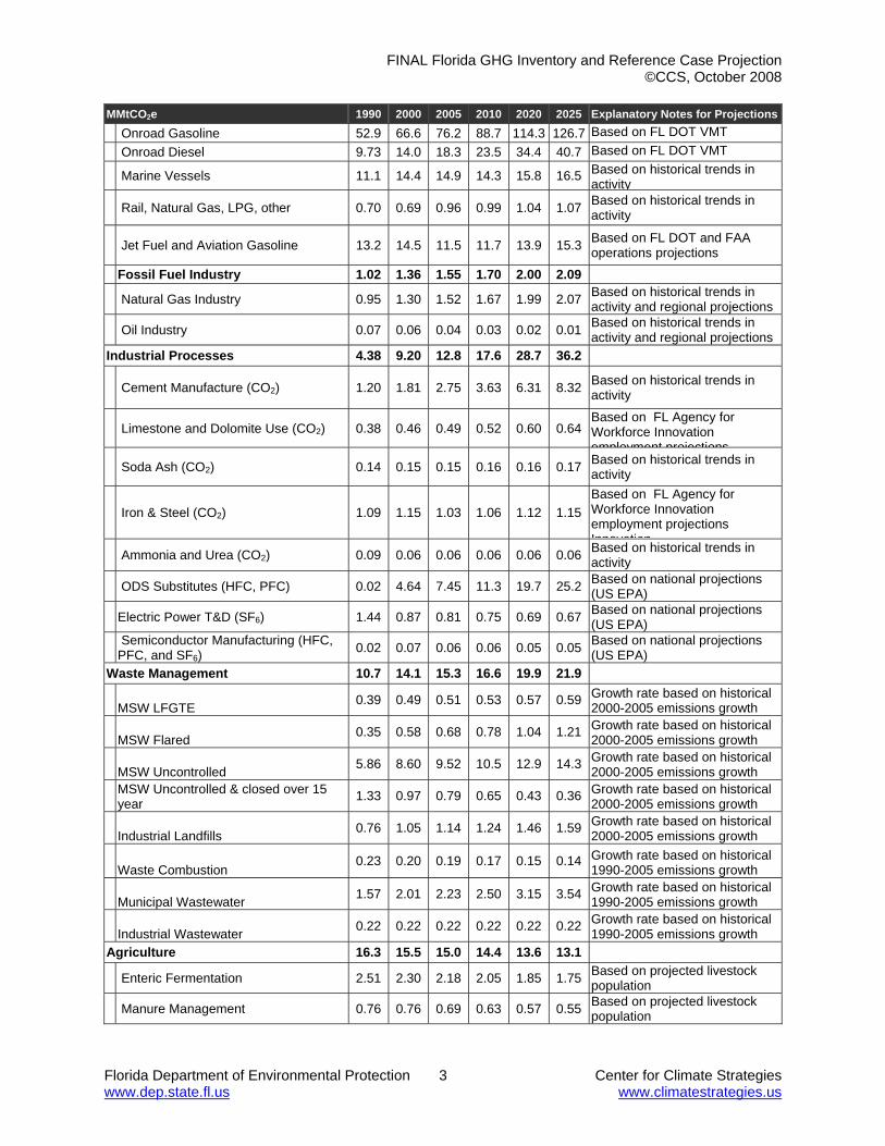
Table 1. Florida Historical and Reference Case GHG Emissions, by Sectora
MMtCO2e 1990 2000 2005 2010 2020 2025 Explanatory Notes for ProjectionsEnergy Use (CO2, CH4, N2O) 210.3 270.9 286.8 307.3 356.0 385.3
Electricity Use (Consumption) 100.6 136.2 142.2 145.0 151.3 158.5Totals include emissions for electricity production plus emissions associated with net imported/exported electricity.
Electricity Production (in-state) 86.1 124.3 134.1 138.5 151.3 158.5 See electric sector ti Coal 54.1 72.3 60.4 69.2 74.4 73.5 in Annex A.
Natural Gas 11.1 22.6 38.0 56.1 68.2 78.4 Oil 20.3 28.1 32.0 9.38 5.10 3.75
Biomass (CH4 and N2O) 0.015 0.010 0.000 0.000 0.000 0.000
MSW/Landfill Gas 0.37 0.74 3.60 3.24 2.89 2.21
Other 0.34 0.48 0.01 0.57 0.74 0.60
Imported/Exported Electricity 14.5 11.9 8.09 6.57 0.00 0.00 Positive values represent net imported electricity
Residential/Commercial/Industrial (RCI) Fuel Use 21.0 23.1 21.2 21.3 23.3 24.4
Coal 2.84 3.02 2.58 2.81 2.83 2.91 Based on US DOE regional projections
Natural Gas 7.73 9.84 7.93 8.15 9.60 10.4 Based on US DOE regional projections
Petroleum 10.1 10.1 10.5 9.86 10.3 10.5 Based on US DOE regional projections
Wood (CH4 and N2O) 0.40 0.21 0.22 0.54 0.60 0.64 Based on US DOE regional projections
Transportation 87.6 110.2 121.8 139.2 179.4 200.3
FINAL Florida GHG Inventory and Reference Case Projection ©CCS, October 2008
Florida Department of Environmental Protection 3 Center for Climate Strategies www.dep.state.fl.us www.climatestrategies.us
MMtCO2e 1990 2000 2005 2010 2020 2025 Explanatory Notes for Projections Onroad Gasoline 52.9 66.6 76.2 88.7 114.3 126.7 Based on FL DOT VMT
j ti Onroad Diesel 9.73 14.0 18.3 23.5 34.4 40.7 Based on FL DOT VMT j ti
Marine Vessels 11.1 14.4 14.9 14.3 15.8 16.5 Based on historical trends in activity
Rail, Natural Gas, LPG, other 0.70 0.69 0.96 0.99 1.04 1.07 Based on historical trends in activity
Jet Fuel and Aviation Gasoline 13.2 14.5 11.5 11.7 13.9 15.3 Based on FL DOT and FAA operations projections
Fossil Fuel Industry 1.02 1.36 1.55 1.70 2.00 2.09
Natural Gas Industry 0.95 1.30 1.52 1.67 1.99 2.07 Based on historical trends in activity and regional projections
Oil Industry 0.07 0.06 0.04 0.03 0.02 0.01 Based on historical trends in activity and regional projections
Industrial Processes 4.38 9.20 12.8 17.6 28.7 36.2
Cement Manufacture (CO2) 1.20 1.81 2.75 3.63 6.31 8.32 Based on historical trends in activity
Limestone and Dolomite Use (CO2) 0.38 0.46 0.49 0.52 0.60 0.64Based on FL Agency for Workforce Innovation employment projections
Soda Ash (CO2) 0.14 0.15 0.15 0.16 0.16 0.17 Based on historical trends in activity
Iron & Steel (CO2) 1.09 1.15 1.03 1.06 1.12 1.15Based on FL Agency for Workforce Innovation employment projections Innovation
Ammonia and Urea (CO2) 0.09 0.06 0.06 0.06 0.06 0.06 Based on historical trends in activity
ODS Substitutes (HFC, PFC) 0.02 4.64 7.45 11.3 19.7 25.2 Based on national projections (US EPA)
Electric Power T&D (SF6) 1.44 0.87 0.81 0.75 0.69 0.67 Based on national projections (US EPA)
Semiconductor Manufacturing (HFC, PFC, and SF6)
0.02 0.07 0.06 0.06 0.05 0.05 Based on national projections (US EPA)
Waste Management 10.7 14.1 15.3 16.6 19.9 21.9
MSW LFGTE 0.39 0.49 0.51 0.53 0.57 0.59 Growth rate based on historical 2000-2005 emissions growth
MSW Flared 0.35 0.58 0.68 0.78 1.04 1.21 Growth rate based on historical 2000-2005 emissions growth
MSW Uncontrolled 5.86 8.60 9.52 10.5 12.9 14.3 Growth rate based on historical 2000-2005 emissions growth
MSW Uncontrolled & closed over 15 year 1.33 0.97 0.79 0.65 0.43 0.36 Growth rate based on historical
2000-2005 emissions growth
Industrial Landfills 0.76 1.05 1.14 1.24 1.46 1.59 Growth rate based on historical 2000-2005 emissions growth
Waste Combustion
0.23 0.20 0.19 0.17 0.15 0.14 Growth rate based on historical 1990-2005 emissions growth
Municipal Wastewater 1.57 2.01 2.23 2.50 3.15 3.54 Growth rate based on historical 1990-2005 emissions growth
Industrial Wastewater 0.22 0.22 0.22 0.22 0.22 0.22 Growth rate based on historical 1990-2005 emissions growth
Agriculture 16.3 15.5 15.0 14.4 13.6 13.1
Enteric Fermentation 2.51 2.30 2.18 2.05 1.85 1.75 Based on projected livestock population
Manure Management 0.76 0.76 0.69 0.63 0.57 0.55 Based on projected livestock population

FINAL Florida GHG Inventory and Reference Case Projection ©CCS, October 2008
Florida Department of Environmental Protection 4 Center for Climate Strategies www.dep.state.fl.us www.climatestrategies.us
MMtCO2e 1990 2000 2005 2010 2020 2025 Explanatory Notes for Projections
Agricultural Soils 3.36 2.73 2.43 2.03 1.43 1.14 Based on historical growth
Agricultural Burning 0.01 0.01 0.01 0.01 0.01 0.01 Based on historical growth
Rice Cultivation 0.06 0.09 0.06 0.06 0.06 0.06 Assumed no change after 2005
Agricultural Soils (cultivation practices) 9.63 9.63 9.63 9.63 9.63 9.63 Based on 1997 USDA Data
Forest Fires (CH4 and N2O) 7.05 5.29 6.82 6.70 6.70 6.70Based on the average of historical wildfire and prescribed fire emissions
Gross Emissions (Consumption Basis, Excludes Sinks) 248.8 315.0 336.6 362.6 424.9 463.3
increase relative to 1990 27% 35% 46% 71% 86% Emissions Sinks -17.8 -26.7 -27.3 -27.2 -27.1 -27.1
Forested Landscape -3.38 -21.1 -21.1 -21.0 -20.9 -20.9 Based on estimates from the USFS
Urban Forestry and Land Use -14.4 -5.65 -6.23 -6.23 -6.23 -6.23 Assumed no change after 2005 Net Emissions (Includes Sinks) 230.9 288.3 309.4 335.3 397.8 436.2 increase relative to 1990 25% 34% 45% 72% 89% a Totals may not equal exact sum of subtotals shown in this table due to independent rounding.
Historical Emissions Overview In 2005, activities in Florida accounted for approximately 337 million metric tons (MMt) of CO2e emissions, an amount equal to about 4.7% of total US GHG emissions.13 Florida’s gross GHG emissions are rising faster than those of the nation as a whole (gross emissions exclude carbon sinks, such as forests). Florida’s gross GHG emissions increased 35% from 1990 to 2005, while national emissions rose by 16% from 1990 to 2005. Figure 1 illustrates the State’s emissions per capita and per unit of economic output.14 On a per capita basis, gross CO2e emissions in 1990 were about 19 metric tons (t) per capita, lower than the 1990 national average of 25 tCO2e per capita. Per capita emissions in Florida changed very little between 1990 and 2005, staying relatively constant at 19 tCO2e per capita in 2005. National per capita emissions decreased slightly to 24 MtCO2e per capita from 1990 to 2005. Like the nation as a whole, Florida’s economic growth exceeded emissions growth throughout the 1990-2005 period, leading to declining estimates of GHG emissions per unit of state product. From 1990 to 2005, emissions per unit of gross product dropped by 26%, both in Florida and nationally.15 13 The national emissions used for these comparisons are based on emissions from Inventory of US Greenhouse Gas Emissions and Sinks: 1990–2006, April 15, 2008, US EPA # 430-R-08-005, http://www.epa.gov/climatechange/emissions/usinventoryreport.html. 14 Florida population data from the Demographic Estimating Conference Database, updated August 2007. http://edr.state.fl.us/population.htm 15 Based on real gross domestic product (millions of chained 2000 dollars) that excludes the affects of inflation, available from the US Bureau of Economic Analysis (http://www.bea.gov/regional/gsp/). The national emissions used for these comparisons are based on 2005 emissions from the 2008 version of EPA’s GHG inventory report (http://www.epa.gov/climatechange/emissions/usinventoryreport.html).

FINAL Florida GHG Inventory and Reference Case Projection ©CCS, October 2008
Florida Department of Environmental Protection 5 Center for Climate Strategies www.dep.state.fl.us www.climatestrategies.us
Figure 1. Historical Florida and US Gross GHG Emissions,
Per Capita and Per Unit Gross Product
0
5
10
15
20
25
30
1990 1995 2000 2005
USGHG/Capita(tCO2e)FLGHG/Capita(tCO2e)US GHG/$(100gCO2e)
FL GHG/$(100gCO2e)
Figure 2 compares the contribution of gross GHG emissions by sector estimated for Florida to emissions for the U.S. by sector for 2005. Principal sources of Florida’s GHG emissions are electricity consumption and the transportation sector, accounting for 42% and 36% of Florida’s gross GHG emissions in 2005, respectively. The portion of emissions from the electricity consumption and transportation sectors is much greater in Florida than the national average of 34% for electricity consumption and 27% for transportation. Activities in the residential, commercial, and industrial (RCI) fuel use16 sectors produce GHG emissions when fuels are combusted to provide space heating, process heating, and other applications. In 2005, combustion of oil, natural gas, coal, and wood in the RCI sectors contributed about 6% (about 21 MMtCO2e) of Florida’s gross GHG emissions, significantly lower than the RCI sector contribution for the nation (22%). The next largest contributor is the agricultural sector, which accounts for 6% of the gross GHG emissions in Florida in 2005. This is slightly lower than the national average for agricultural emissions in that year (8%). Forest fires, including wildfires and prescribed burns, are included in this sector in Figure 2 for both Florida and the US. Although the contribution from forest fire emissions is minimal for the nation as a whole, accounting for less than 0.2% of gross GHG emissions, forest fire emissions in Florida account for 2% of gross emissions in 2005. The majority of agricultural emissions in Florida come from the cultivation of agricultural soils. While the industrial processes sector accounted for 4% of gross GHG emissions in 2005, emissions in this sector are increasing rapidly, at an annual growth rate of 5% per year from 2005 16 The industrial sector includes emissions associated with agricultural energy use and fuel used by the fossil fuel production industry.

FINAL Florida GHG Inventory and Reference Case Projection ©CCS, October 2008
Florida Department of Environmental Protection 6 Center for Climate Strategies www.dep.state.fl.us www.climatestrategies.us
to 2025. This results in the contribution of the industrial processes sector accounting for an estimated 8% of Florida’s gross GHG emissions by 2025.17 Industrial process emissions are rising primarily due to the increasing use of HFCs as substitutes for ozone-depleting chlorofluorocarbons (CFCs). Other industrial process emissions result from CO2 released during production of cement, iron and steel, and ammonia, and the use of urea, soda ash, limestone, and dolomite. In addition, SF6 is released in the use of electric power transmission and distribution (T&D) equipment, while semiconductor manufacturing is responsible for the release of HFCs, PFCs, and SF6. Waste management accounted for about 5% of Florida’s gross GHG emissions in 2005. These emissions are primarily associated with the release of CH4 from landfills, as well as from CO2 and N2O associated with solid waste incineration and residential open burning, and CH4 and N2O emissions associated with wastewater management. The fossil fuel industry category accounted for 0.5% of Florida’s gross GHG emissions in 2005. This category includes methane emissions associated with natural gas production, processing, T&D, flaring, and pipeline fuel use, as well as with oil production and refining (included under the fossil fuel industry category).
Figure 2. Gross GHG Emissions by Sector, 2005, Florida and US
US Transport27%
Waste3%
Agriculture andForest Fires
7%
Electricity34%
Industrial Process
4%
Fossil Fuel Industry
3%
Res/Com Fuel Use
8%
Industrial Fuel Use
14%
A Closer Look at the Two Major Sources: Electricity Consumption and the Transportation Sectors
Electricity Supply Sector
17 CFCs are also potent GHGs; they are not, however, included in GHG estimates because of concerns related to implementation of the Montreal Protocol (See Annex I for additional information). HFCs are used as refrigerants in the RCI and transport sectors as well as in the industrial sector; they are included here, however, within the industrial processes emissions.
FINAL Florida GHG Inventory and Reference Case Projection ©CCS, October 2008
Florida Department of Environmental Protection 7 Center for Climate Strategies www.dep.state.fl.us www.climatestrategies.us
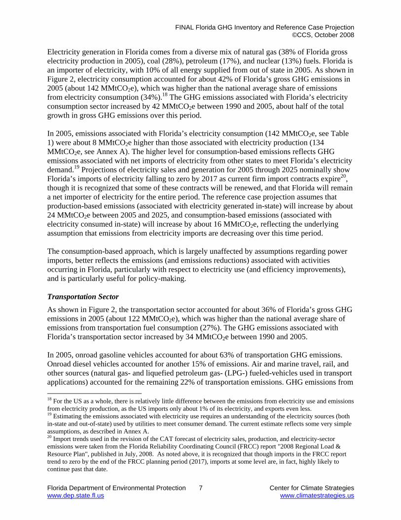
Electricity generation in Florida comes from a diverse mix of natural gas (38% of Florida gross electricity production in 2005), coal (28%), petroleum (17%), and nuclear (13%) fuels. Florida is an importer of electricity, with 10% of all energy supplied from out of state in 2005. As shown in Figure 2, electricity consumption accounted for about 42% of Florida’s gross GHG emissions in 2005 (about 142 MMtCO2e), which was higher than the national average share of emissions from electricity consumption (34%).18 The GHG emissions associated with Florida’s electricity consumption sector increased by 42 MMtCO2e between 1990 and 2005, about half of the total growth in gross GHG emissions over this period. In 2005, emissions associated with Florida’s electricity consumption (142 MMtCO2e, see Table 1) were about 8 MMtCO2e higher than those associated with electricity production (134 MMtCO2e, see Annex A). The higher level for consumption-based emissions reflects GHG emissions associated with net imports of electricity from other states to meet Florida’s electricity demand.19 Projections of electricity sales and generation for 2005 through 2025 nominally show Florida’s imports of electricity falling to zero by 2017 as current firm import contracts expire20, though it is recognized that some of these contracts will be renewed, and that Florida will remain a net importer of electricity for the entire period. The reference case projection assumes that production-based emissions (associated with electricity generated in-state) will increase by about 24 MMtCO2e between 2005 and 2025, and consumption-based emissions (associated with electricity consumed in-state) will increase by about 16 MMtCO2e, reflecting the underlying assumption that emissions from electricity imports are decreasing over this time period. The consumption-based approach, which is largely unaffected by assumptions regarding power imports, better reflects the emissions (and emissions reductions) associated with activities occurring in Florida, particularly with respect to electricity use (and efficiency improvements), and is particularly useful for policy-making. Transportation Sector As shown in Figure 2, the transportation sector accounted for about 36% of Florida’s gross GHG emissions in 2005 (about 122 MMtCO2e), which was higher than the national average share of emissions from transportation fuel consumption (27%). The GHG emissions associated with Florida’s transportation sector increased by 34 MMtCO2e between 1990 and 2005. In 2005, onroad gasoline vehicles accounted for about 63% of transportation GHG emissions. Onroad diesel vehicles accounted for another 15% of emissions. Air and marine travel, rail, and other sources (natural gas- and liquefied petroleum gas- (LPG-) fueled-vehicles used in transport applications) accounted for the remaining 22% of transportation emissions. GHG emissions from 18 For the US as a whole, there is relatively little difference between the emissions from electricity use and emissions from electricity production, as the US imports only about 1% of its electricity, and exports even less. 19 Estimating the emissions associated with electricity use requires an understanding of the electricity sources (both in-state and out-of-state) used by utilities to meet consumer demand. The current estimate reflects some very simple assumptions, as described in Annex A. 20 Import trends used in the revision of the CAT forecast of electricity sales, production, and electricity-sector emissions were taken from the Florida Reliability Coordinating Council (FRCC) report "2008 Regional Load & Resource Plan", published in July, 2008. As noted above, it is recognized that though imports in the FRCC report trend to zero by the end of the FRCC planning period (2017), imports at some level are, in fact, highly likely to continue past that date.

FINAL Florida GHG Inventory and Reference Case Projection ©CCS, October 2008
Florida Department of Environmental Protection 8 Center for Climate Strategies www.dep.state.fl.us www.climatestrategies.us
onroad gasoline use increased 44% between 1990 and 2005. Meanwhile, GHG emissions from onroad diesel use rose 88% during that period. Emissions associated with marine fuel use increased by about 35% from 1990 to 2005, while emissions associated with aviation fuel consumption decreased by 13% in the same period.
From 1990 through 2005, Florida’s GHG emissions from transportation fuel use have risen steadily at an average rate of about 2.2% annually. During the period from 2005 to 2025, emissions from transportation fuels are projected to rise at a rate of 2.5% per year. This leads to an increase of 78 MMtCO2e in transportation emissions from 2005 to 2025. The largest percentage increase in emissions over this time period is seen in onroad diesel fuel consumption, which is projected to increase by 123% from 2005 to 2025.
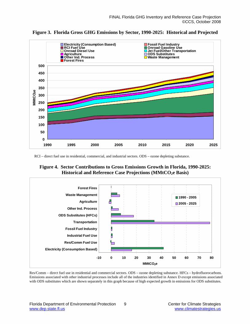
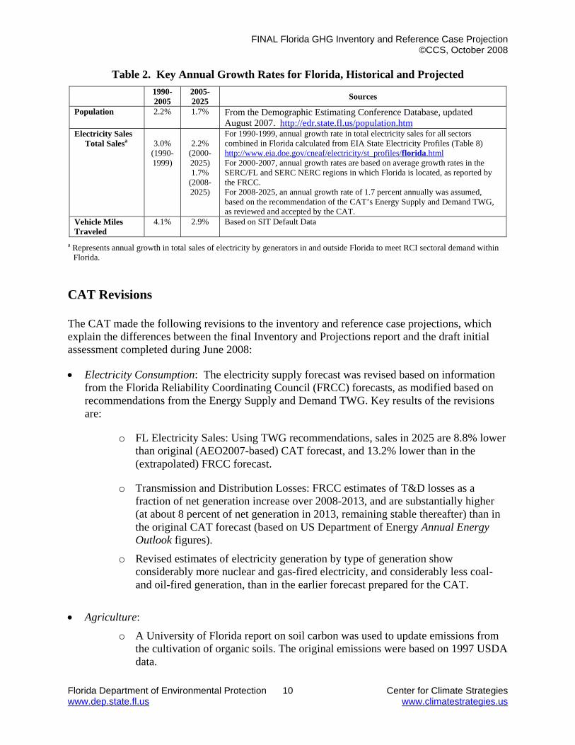
Reference Case Projections (Business as Usual) Relying on a variety of sources for projections, as noted below and in the appendices, we developed a simple reference case projection of GHG emissions through 2025. As illustrated in Figure 3 and shown numerically in Table 1, under the reference case projections, Florida gross GHG emissions continue to grow steadily, climbing to about 463 MMtCO2e by 2025, 86% above 1990 levels. This equates to a 1.6% annual rate of growth from 2005 to 2025. The transportation sector is projected to be the largest contributor to future emissions growth, followed by emissions associated with the increasing use of HFCs and PFCs as substitutes for ozone-depleting substances (ODS) in refrigeration, air conditioning, and other applications. Other sources of emissions growth include electricity consumption, as well as the waste management sector, as shown in Figure 4. Table 2 summarizes the growth rates that drive the growth in the Florida reference case projections, as well as the sources of these data.
FINAL Florida GHG Inventory and Reference Case Projection ©CCS, October 2008
Florida Department of Environmental Protection 9 Center for Climate Strategies www.dep.state.fl.us www.climatestrategies.us
Figure 3. Florida Gross GHG Emissions by Sector, 1990-2025: Historical and Projected
0
50
100
150
200
250
300
350
400
450
500
1990 1995 2000 2005 2010 2015 2020 2025
MM
tCO 2
e
Electricity (Consumption Based) Fossil Fuel IndustryRCI Fuel Use Onroad Gasoline UseOnroad Diesel Use Jet Fuel/Other TransportationAgriculture ODS SubstitutesOther Ind. Process Waste ManagementForest Fires
RCI – direct fuel use in residential, commercial, and industrial sectors. ODS – ozone depleting substance.
Figure 4. Sector Contributions to Gross Emissions Growth in Florida, 1990-2025: Historical and Reference Case Projections (MMtCO2e Basis)
-10 0 10 20 30 40 50 60 70 80
Electricity (Consumption Based)
Res/Comm Fuel Use
Industrial Fuel Use
Fossil Fuel Industry
Transportation
ODS Substitutes (HFCs)
Other Ind. Process
Agriculture
Waste Management
Forest Fires
MMtCO2e
1990 - 2005
2005 - 2025
Res/Comm – direct fuel use in residential and commercial sectors. ODS – ozone depleting substance. HFCs – hydrofluorocarbons. Emissions associated with other industrial processes include all of the industries identified in Annex D except emissions associated with ODS substitutes which are shown separately in this graph because of high expected growth in emissions for ODS substitutes.
FINAL Florida GHG Inventory and Reference Case Projection ©CCS, October 2008
Florida Department of Environmental Protection 10 Center for Climate Strategies www.dep.state.fl.us www.climatestrategies.us
Table 2. Key Annual Growth Rates for Florida, Historical and Projected 1990-
2005 2005-2025 Sources
Population 2.2% 1.7% From the Demographic Estimating Conference Database, updated August 2007. http://edr.state.fl.us/population.htm
Electricity Sales Total Salesa
3.0%
(1990-1999)
2.2%
(2000-2025) 1.7%
(2008-2025)
For 1990-1999, annual growth rate in total electricity sales for all sectors combined in Florida calculated from EIA State Electricity Profiles (Table 8) http://www.eia.doe.gov/cneaf/electricity/st_profiles/florida.html For 2000-2007, annual growth rates are based on average growth rates in the SERC/FL and SERC NERC regions in which Florida is located, as reported by the FRCC. For 2008-2025, an annual growth rate of 1.7 percent annually was assumed, based on the recommendation of the CAT’s Energy Supply and Demand TWG, as reviewed and accepted by the CAT.
Vehicle Miles Traveled
4.1% 2.9% Based on SIT Default Data
a Represents annual growth in total sales of electricity by generators in and outside Florida to meet RCI sectoral demand within Florida.
CAT Revisions The CAT made the following revisions to the inventory and reference case projections, which explain the differences between the final Inventory and Projections report and the draft initial assessment completed during June 2008:
• Electricity Consumption: The electricity supply forecast was revised based on information from the Florida Reliability Coordinating Council (FRCC) forecasts, as modified based on recommendations from the Energy Supply and Demand TWG. Key results of the revisions are:
o FL Electricity Sales: Using TWG recommendations, sales in 2025 are 8.8% lower than original (AEO2007-based) CAT forecast, and 13.2% lower than in the (extrapolated) FRCC forecast.
o Transmission and Distribution Losses: FRCC estimates of T&D losses as a fraction of net generation increase over 2008-2013, and are substantially higher (at about 8 percent of net generation in 2013, remaining stable thereafter) than in the original CAT forecast (based on US Department of Energy Annual Energy Outlook figures).
o Revised estimates of electricity generation by type of generation show considerably more nuclear and gas-fired electricity, and considerably less coal- and oil-fired generation, than in the earlier forecast prepared for the CAT.
• Agriculture:
o A University of Florida report on soil carbon was used to update emissions from the cultivation of organic soils. The original emissions were based on 1997 USDA data.

FINAL Florida GHG Inventory and Reference Case Projection ©CCS, October 2008
Florida Department of Environmental Protection 11 Center for Climate Strategies www.dep.state.fl.us www.climatestrategies.us
• Waste Management:
o Florida DEP provided supplemental landfill facilities information to update the data from EPA’s Landfill Methane Outreach Program (LMOP). Gaps in activity data were augmented with average values and assumptions (described in Annex G).
o Solid waste landfills and emissions were separated into five groups: MSW Landfill Gas to Energy, MSW Flared, MSW Uncontrolled, MSW Uncontrolled and Closed Over 15 Years, and Industrial Landfills.
o Historical (2000-2005) growth in emissions from landfills were used as growth rates for projecting 2006-2025 emissions from waste landfilled.
• Forestry and Land Use:
o The Agriculture, Forestry, and Waste TWG group provided an updated USFS report, Florida’s Forests – 1995, which was used to revise historical forest carbon flux values for 1987-1995 and 1995-2005.
o Projections in forest land carbon flux (2005-2025) were originally kept at 2005
levels. The revised projections take into account annual forest area losses based on USFS reports: Florida’s Forests – 1995 and Florida’s Forests - 2005.
o In addition to wildfire emissions, Florida Division of Forestry provided activity
data for prescribed burning, which increased the overall emissions from forest fires. Also, forest fires emission forecasts were revised to reflect historic average emissions; this was done due to uncertainty in future forest fire projections and wide annual fluctuations in acres of forest area burned.
Reference Case Projections With Recent Actions21 During the Florida Climate Action Team process, the CAT identified a number of recent actions that Florida has undertaken to control GHG emissions while at the same time conserving energy and promoting the development and use of renewable energy sources. A total of four recent actions were identified for which data were available to estimate the emission reductions of the actions relative to the business-as-usual reference case projections. The GHG emission reductions projected to be achieved by these actions are summarized in Table 3. This table shows a total reduction of about 109 MMtCO2e in 2025 from the business-as-usual reference case emissions, or a 23% reduction from the business-as-usual emissions in 2025 for all sectors combined. Figure 5 illustrates the emission reductions associated with each of the recent actions analyzed. Table 3 provides the numeric estimates underlying Figure 5.
21 Note that actions recently adopted by the state of Florida have also been referred to as “existing” actions.

FINAL Florida GHG Inventory and Reference Case Projection ©CCS, October 2008
Florida Department of Environmental Protection 12 Center for Climate Strategies www.dep.state.fl.us www.climatestrategies.us
Figure 5. Florida Emission Reductions from Recent Actions
050
100150200250300350400450500
1990 1995 2000 2005 2010 2015 2020 2025
MM
tCO
2e
BAU Emissions Utility CapCalifornia Clean Car Stds Statewide Diesel Idling StdBuilding Efficiency Improvements Appliance Efficiency ImprovementsBuilding Codes for Energy Efficiency Target Emission Levels
The following provides a brief summary of each of the four recent actions.
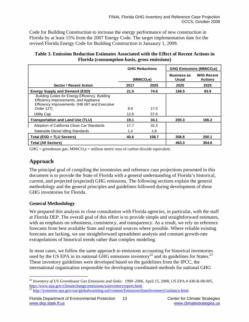
Electric Utility Cap: Section 2 of the Executive Order 127 established a maximum allowable emissions level of GHG for electric utilities in Florida. The standard will require milestone reductions in three key years--by 2017, emissions must not be greater than 2000 utility sector emissions; by 2025, emissions must not be greater than utility sector emissions; and by 2050, emissions must not be greater than 20% of 1990 utility sector emissions. Adopt CA Clean Car Standards: Section 2 of the Executive Order 127 calls for the adoption of the California motor vehicle emissions standards in Title 13 of the California Code of Regulations, effective January 1, 2005, upon approval by the EPA of a pending waiver. The California standards incorporate the main global warming gases—CO2, methane, and nitrous oxide—resulting directly from vehicle operation (tailpipe emissions), as well as hydrofluorocarbon emissions resulting from leakage from or operation of vehicle air conditioning systems. Statewide Diesel Idling Standards: Section 2 of the Executive Order 127 established the adoption of a statewide diesel engine idle reduction standard. Building Codes for Energy Efficiency: Section 2 of the Executive Order 127 calls for the convening of the Florida Building Commission for the purpose of revising the Florida Energy
FINAL Florida GHG Inventory and Reference Case Projection ©CCS, October 2008
Florida Department of Environmental Protection 13 Center for Climate Strategies www.dep.state.fl.us www.climatestrategies.us
Code for Building Construction to increase the energy performance of new construction in Florida by at least 15% from the 2007 Energy Code. The target implementation date for the revised Florida Energy Code for Building Construction is Januaury 1, 2009.
Table 3. Emission Reduction Estimates Associated with the Effect of Recent Actions in Florida (consumption-basis, gross emissions)
Sector / Recent Action
GHG Reductions GHG Emissions (MMtCO2e)
(MMtCO2e) Business as
Usual With Recent
Actions 2017 2025 2025 2025
Energy Supply and Demand (ESD) 21.5 74.6 158.5 83.9 Building Codes for Energy Efficiency, Building Efficiency Improvements, and Appliance Efficiency Improvements (HB 697 and Executive Order 127) 8.9 17.0 Utility Cap 12.6 57.6
Transportation and Land Use (TLU) 19.1 34.1 200.3 166.2 Adoption of California Clean Car Standards 17.7 32.3 Statewide Diesel Idling Standards 1.4 1.8
Total (ESD + TLU Sectors) 40.6 108.7 358.8 250.1 Total (All Sectors) 463.3 354.6
GHG = greenhouse gas; MMtCO2e = million metric tons of carbon dioxide equivalent.
Approach The principal goal of compiling the inventories and reference case projections presented in this document is to provide the State of Florida with a general understanding of Florida’s historical, current, and projected (expected) GHG emissions. The following sections explain the general methodology and the general principles and guidelines followed during development of these GHG inventories for Florida. General Methodology
We prepared this analysis in close consultation with Florida agencies, in particular, with the staff at Florida DEP. The overall goal of this effort is to provide simple and straightforward estimates, with an emphasis on robustness, consistency, and transparency. As a result, we rely on reference forecasts from best available State and regional sources where possible. Where reliable existing forecasts are lacking, we use straightforward spreadsheet analysis and constant growth-rate extrapolations of historical trends rather than complex modeling. In most cases, we follow the same approach to emissions accounting for historical inventories used by the US EPA in its national GHG emissions inventory22 and its guidelines for States.23 These inventory guidelines were developed based on the guidelines from the IPCC, the international organization responsible for developing coordinated methods for national GHG
22 Inventory of US Greenhouse Gas Emissions and Sinks: 1990–2006, April 15, 2008, US EPA # 430-R-08-005, http://www.epa.gov/climatechange/emissions/usinventoryreport.html. 23 http://yosemite.epa.gov/oar/globalwarming.nsf/content/EmissionsStateInventoryGuidance.html.

FINAL Florida GHG Inventory and Reference Case Projection ©CCS, October 2008
Florida Department of Environmental Protection 14 Center for Climate Strategies www.dep.state.fl.us www.climatestrategies.us
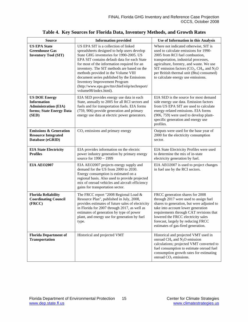
inventories.24 The inventory methods provide flexibility to account for local conditions. The key sources of activity and projection data used are shown in Table 4. Table 4 also provides the descriptions of the data provided by each source and the uses of each data set in this analysis. General Principles and Guidelines A key part of this effort involves the establishment and use of a set of generally accepted accounting principles for evaluation of historical and projected GHG emissions, as follows:
• Transparency: We report data sources, methods, and key assumptions to allow open
review and opportunities for additional revisions later based on input from others. In addition, we report key uncertainties where they exist.
• Consistency: To the extent possible, the inventory and projections were designed to be
externally consistent with current or likely future systems for State and national GHG emission reporting. We have used the EPA tools for State inventories and projections as a starting point. These initial estimates were then augmented and/or revised as needed to conform with State-based inventory and base-case projection needs. For consistency in making reference case projections, we define reference case actions for the purposes of projections as those currently in place or reasonably expected over the time period of analysis.
• Priority of Existing State and Local Data Sources: In gathering data and in cases
where data sources conflicted, we placed highest priority on local and State data and analyses, followed by regional sources, with national data or simplified assumptions such as constant linear extrapolation of trends used as defaults where necessary.
• Priority of Significant Emissions Sources: In general, activities with relatively small
emissions levels may not be reported with the same level of detail as other activities.
• Comprehensive Coverage of Gases, Sectors, State Activities, and Time Periods: This analysis aims to comprehensively cover GHG emissions associated with activities in Florida. It covers all six GHGs covered by US and other national inventories: CO2, CH4, N2O, SF6, HFCs, and PFCs. The inventory estimates are for the year 1990, with subsequent years included up to most recently available data (typically 2001 to 2005), with projections to 2025.
• Use of Consumption-Based Emissions Estimates: To the extent possible, we estimated
emissions that are caused by activities that occur in Florida. For example, we reported emissions associated with the electricity consumed in Florida. The rationale for this method of reporting is that it can more accurately reflect the impact of State-based policy strategies such as energy efficiency on overall GHG emissions, and it resolves double-counting and exclusion problems with multi-emissions issues. This approach can differ from how inventories are compiled, for example, on an in-state production basis, in particular for electricity.
24 http://www.ipcc-nggip.iges.or.jp/public/gl/invs1.htm.
FINAL Florida GHG Inventory and Reference Case Projection ©CCS, October 2008
Florida Department of Environmental Protection 15 Center for Climate Strategies www.dep.state.fl.us www.climatestrategies.us
Table 4. Key Sources for Florida Data, Inventory Methods, and Growth Rates Source Information provided Use of Information in this Analysis
US EPA State Greenhouse Gas Inventory Tool (SIT)
US EPA SIT is a collection of linked spreadsheets designed to help users develop State GHG inventories for 1990-2005. US EPA SIT contains default data for each State for most of the information required for an inventory. The SIT methods are based on the methods provided in the Volume VIII document series published by the Emissions Inventory Improvement Program (http://www.epa.gov/ttn/chief/eiip/techreport/volume08/index.html).
Where not indicated otherwise, SIT is used to calculate emissions for 1990-2005 from RCI fuel combustion, transportation, industrial processes, agriculture, forestry, and waste. We use SIT emission factors (CO2, CH4, and N2O per British thermal unit (Btu) consumed) to calculate energy use emissions.
US DOE Energy Information Administration (EIA) forms; State Energy Data (SED)
EIA SED provides energy use data in each State, annually to 2005 for all RCI sectors and fuels and for transportation fuels. EIA forms (759, 906) provide generation and primary energy use data at electric power generators.
EIA SED is the source for most demand side energy use data. Emission factors from US EPA SIT are used to calculate energy-related emissions. EIA forms (906, 759) were used to develop plant-specific generation and energy use profiles.
Emissions & Generation Resource Integrated Database (eGRID)
CO2 emissions and primary energy Outputs were used for the base year of 2000 for the electricity consumption sector.
EIA State Electricity Profiles
EIA provides information on the electric power industry generation by primary energy source for 1990 – 1999
EIA State Electricity Profiles were used to determine the mix of in-state electricity generation by fuel.
EIA AEO2007
EIA AEO2007 projects energy supply and demand for the US from 2000 to 2030. Energy consumption is estimated on a regional basis. Also used to provide projected mix of onroad vehicles and aircraft efficiency gains for transportation sector.
EIA AEO2007 is used to project changes in fuel use by the RCI sectors.
Florida Reliability Coordinating Council (FRCC)
The FRCC report "2008 Regional Load & Resource Plan", published in July, 2008, provides estimates of future sales of electricity in Florida for 2007 through 2017, as well as estimates of generation by type of power plant, and energy use for generation by fuel type.
FRCC generation shares for 2008 through 2017 were used to assign fuel shares to generation, but were adjusted to take into account lower generation requirements through CAT revisions that lowered the FRCC electricity sales forecast, largely by reducing FRCC estimates of gas-fired generation.
Florida Department of Transportation
Historical and projected VMT Historical and projected VMT used in onroad CH4 and N2O emission calculations; projected VMT converted to fuel consumption to estimate onroad fuel consumption growth rates for estimating onroad CO2 emissions.

FINAL Florida GHG Inventory and Reference Case Projection ©CCS, October 2008
Florida Department of Environmental Protection 16 Center for Climate Strategies www.dep.state.fl.us www.climatestrategies.us
Source Information provided Use of Information in this Analysis US Department of Transportation (DOT), Office of Pipeline Safety (OPS)
Natural gas transmission pipeline mileage for 2001-2005 (pre-2001 mileage estimated based on 1990-2001 trend in volume of natural gas transported into/out of Florida as reported by the Energy Information Administration [EIA]).
Entered into SIT to calculate historical emissions. Transmission pipeline emissions projected based on smallest annualized growth in Florida gathering/transmission emissions (+1.93%) from each of 3 periods analyzed (1990-2005; 1995-2005; and 2000-2005).
PennWell Corporation Oil and Gas Journal
Number of gas processing plants in Florida for 1990-2005.
PennWell data entered into SIT to calculate historical emissions. Emissions projected assuming no change from 2005 levels because there has been a constant number of plants for the last 11 years.
Florida Department of Environmental Protection
Number of associated wells for 1990-2005. Natural gas gathering pipeline mileage for 2005 (pre-2005 mileage estimated based on 1990-2005 trend in Florida natural gas production as reported by the EIA).
Well counts entered into SIT to calculate historical emissions. Projections based on smallest annualized decrease in number of Florida wells (-3.57%) from each of 3 historical periods analyzed. Mileage entered into SIT to calculate historical emissions. Projections based on smallest annualized growth in Florida gathering/transmission emissions (1.93%) from each of 3 historical periods analyzed.
Florida Public Service Commission
Number of natural gas transmission compressor stations for 2005 (pre-2005 based on 1990-2005 trend in volume of natural gas transported into/out of Florida as reported by EIA).
Entered into SIT to calculate historical emissions. Transmission compressor station emissions projected based on smallest annualized growth in Florida gathering/transmission emissions (1.93%) from each of 3 historical periods analyzed.
EIA Natural Gas Navigator
Amount of gas flared and vented in Florida for 1990-2005.
Natural Gas Navigator data entered into SIT to calculate historical emissions. Gas well emissions assumed zero throughout forecast period because no venting/flaring reported in Florida for last 11 years
US Forest Service Data on forest carbon stocks for multiple years.
Data are used to calculate CO2 flux over time (terrestrial CO2 sequestration in forested areas).
USDS National Agricultural Statistics Service (NASS)
USDA NASS provides data on crops and livestock.
Crop production data used in SIT to estimate agricultural residue and agricultural soils emissions; livestock population data used in SIT to estimate manure and enteric fermentation emissions.
For electricity, we estimate, in addition to the emissions due to fuels combusted at electricity plants in the State, the emissions related to electricity consumed in Florida. This entails accounting for the electricity sources used by Florida utilities to meet consumer demands. As this analysis is refined in the future, one could also attempt to estimate other sectoral emissions on a consumption basis, such as accounting for emissions from transportation fuel used in Florida, but

FINAL Florida GHG Inventory and Reference Case Projection ©CCS, October 2008
Florida Department of Environmental Protection 17 Center for Climate Strategies www.dep.state.fl.us www.climatestrategies.us
purchased out-of-state. In some cases, this can require venturing into the relatively complex terrain of life-cycle analysis. In general, we recommend considering a consumption-based approach where it will significantly improve the estimation of the emissions impact of potential mitigation strategies. For example re-use, recycling, and source reduction can lead to emission reductions resulting from lower energy requirements for material production (such as paper, cardboard, and aluminum), even though production of those materials, and emissions associated with materials production, may not occur within the State. Details on the methods and data sources used to construct the inventories and forecasts for each source sector are provided in the following appendices:
• Annex A. Electricity Use and Supply • Annex B. Residential, Commercial, and Industrial (RCI) Fuel Combustion • Annex C. Transportation Energy Use • Annex D. Industrial Processes • Annex E. Fossil Fuel Extraction and Distribution Industry • Annex F. Agriculture • Annex G. Waste Management • Annex H. Forestry
Annex I provides additional background information from the US EPA on GHGs and global warming potential values.
Key Uncertainties and Next Steps Some data gaps exist in this inventory, and particularly in the reference case projections. Key tasks for future refinement of this inventory and forecast include review and revision of key drivers, such as the transportation, electricity demand, and waste management growth rates that will be major determinants of Florida’s future GHG emissions (See Table 2 and Figure 4). These growth rates are driven by uncertain economic, demographic and land use trends (including growth patterns and transportation system impacts), all of which deserve closer review and discussion.
DRAFT Florida GHG Inventory and Reference Case Projection ©CCS, October 2008
Florida Department of Environmental Protection 1 Center for Climate Strategies www.dep.state.fl.us www.climatestrategies.us
Annex A. Electricity Supply and Use
Overview This Annex describes the data sources, key assumptions, and the methodology used to develop an inventory of greenhouse gas (GHG) emissions associated with the generation of electricity to meet electricity demand in Florida. The GHG inventory is provided for three periods: 1990-2000, 2001-2006 and 2007-2025. This Annex also describes the data sources, key assumptions, and methodology used to develop a forecast of GHG emissions over the 2007-2025 period associated with meeting electricity demand in the state. As explained in more detail later in this Annex, the approach to calculating emissions for the 1990-2000 time period is primarily based on data from the US Department of Energy (DOE) Energy Information Administration (EIA) and Federal Energy Regulatory Commission (FERC). The 2001-2006 inventory is based in part on data for electricity sales and net generation for load from the Florida Reliability Coordinating Council (FRCC25), and in part on historical electricity output by type of fuel as described in USDOE EIA data26. As the data for total electricity sales between 2001 and 2006 available from EIA and data presented in the FRCC report do not match exactly (the FRCC reports sales totals that are between 1 and 1.5% lower than the EIA data for 2001-2006), sales results for these years should be considered approximate.
For the GHG inventory for the year 2007, the results are based on FRCC data. For the years 2008 through 2025, electricity sales are assumed to increase at an annual rate of 1.7%, a value chosen as representative of recent trends by the Climate Action Team. Net generation required in these years was estimated by adding transmission and distribution (T&D) losses at rates derived from FRCC data (starting at 7.42% of net generation in 2007, and rising to 8.02% of net generation by 2013), but T&D losses assumed to remain at 2013 levels for the duration of the forecast. FRCC data on imports of electrical energy to Florida—which assume that imports decline to zero by 2017 as existing long-term contracts expire27, were also inputs to the estimation of net generation requirements.
FRCC data for electricity output by fuel were used to estimate output by fuel in the years 2008 through 2017 except that, at the direction of the Action Team, generation from solar photovoltaic/solar thermal power plants expected to come on line between 2010 and 2011 was added to the generation mix, and natural gas generation in each year after 2008 was reduced to meet requirements for net generation. For the years 2018 through 2025, the CAT forecast period after the FRCC forecast ends, FRCC trends for generation share for coal, petroleum, and renewables generation for the years 2012 through 2017 were used to extrapolate estimates of generation by those fuels. The same approach was used to extrapolate nuclear generation through
25 Florida Reliability Coordinating Council (FRCC) report 2008 Regional Load & Resource Plan, published in July 2008, and including utility forecasts as filed through April 15, 2008. 26 See, for example, USDOE EIA, “Net Generation by State by Type of Producer by Energy Source, 1990-2006”, Florida entries, available at http://www.eia.doe.gov/cneaf/electricity/epa/generation_state.xls. 27 Input from electricity sector experts in Florida suggests that this assumption is unlikely to be strictly correct, as some, if not many, long-term power import contracts will in fact be renewed. As the emissions associated with imports are also counted in this forecast, this assumption, however, is expected to have little impact on the calculated emissions from electricity generation in Florida.
DRAFT Florida GHG Inventory and Reference Case Projection ©CCS, October 2008
Florida Department of Environmental Protection 2 Center for Climate Strategies www.dep.state.fl.us www.climatestrategies.us
2022, after which nuclear output was assumed, based on Action Team input, to remain steady at just under 67 TWh/yr. Natural gas generation in 2018 through 2025 was adjusted to meet total net generation requirements.
The following topics are covered in this Annex:
Data sources: This section provides an overview of the data sources that were used to develop the inventory and forecast, including publicly accessible websites where this information can be obtained and verified.
Greenhouse Gas Inventory Methodology: This section provides an overview of the methodological approach used to develop the Florida GHG inventory for the electric supply sector.
Greenhouse Gas Inventory Results: This section provides an overview of key results of the Florida GHG inventory for the electric supply sector.
Greenhouse Gas Forecast Methodology: This section provides an overview of the methodological approach used to develop the Florida GHG reference case projections (forecast) for the electric supply sector.
Greenhouse Gas Forecast Results: This section provides an overview of key results of the Florida GHG forecast for the electric supply sector.
GHG Inventory Data Sources for the Period 1990-2006 We considered several sources of information in the development of the inventory and forecast of carbon dioxide equivalent (CO2e) emissions from Florida power plants for the 1990-2006 period. These are briefly summarized below:
2005 EIA-906/920 Monthly Time Series data. This is a database file available from the EIA of the US DOE. The information in the database is based on information collected from utilities in Forms EIA-906/920 and EIA-860. Data from these forms provide, among other things, fuel consumption and net generation in power stations by plant type. This information can be accessed from http://www.eia.doe.gov/cneaf/electricity/page/eia906_920.html.
Monthly Cost and Quality of Fuels for Electric Plants. This information is available from FERC. The database relies on information collected from utilities in the FERC-423 form. It was used to determine the share of coal type (i.e., whether bituminous, sub-bituminous, anthracite, or lignite) as well as the coal quantity consumed in Florida power plants over the period 1990-1999. It can be accessed directly from http://www.eia.doe.gov/cneaf/electricity/page/ferc423.html.
State Electricity Profiles. This information is available from the EIA. The database compiles capacity, net generation, and total retail electricity sales by state. It was used to determine total sales of electricity across all sectors in the base year. It can be accessed directly from http://www.eia.doe.gov/cneaf/electricity/st_profiles/e_profiles_sum.html.
Energy conversion factors. This is based on Table Y-2 of Appendix Y in the USEPA’s 2003 GHG Inventory for the US. The table is entitled “Conversion Factors to Energy Units (Heat Equivalents)”. This information can be accessed directly from the following website: http://yosemite.epa.gov/oar/globalwarming.nsf/UniqueKeyLookup/LHOD5MJTCL/$File/2003-final-inventory_annex_y.pdf.

DRAFT Florida GHG Inventory and Reference Case Projection ©CCS, October 2008
Florida Department of Environmental Protection 3 Center for Climate Strategies www.dep.state.fl.us www.climatestrategies.us
Fuel combustion oxidation factors: This is based on Appendix A of the USEPA’s 2003 US GHG inventory for the US. This information can be accessed directly from: http://www.epa.gov/climatechange/emissions/downloads06/06_Annex_Chapter2.pdf.
Carbon dioxide (CO2), methane (CH4), and nitrous oxide (N2O) emission factors. For all fuels except Municipal Solid Waste (MSW), these emission factors are based on Appendix A of the USEPA’s 2003 GHG inventory for the US. This information can be accessed directly from: http://www.epa.gov/climatechange/emissions/downloads06/06_Annex_Chapter2.pdf. For MSW, emission factors are based on the EIA’s Office of Integrated Analysis and Forecasting, Voluntary Reporting of Greenhouse Gases Program, Table of Fuel and Energy Source: Codes and Emission Coefficients. This information can be accessed directly from http://www.eia.doe.gov/oiaf/1605/coefficients.html.
Global warming potentials: These are based on values proposed by the Intergovernmental Panel on Climate Change (IPCC) Second Assessment Report. This information can be accessed directly from http://www.ipcc.ch/ipccreports/assessments-reports.htm.
GHG Inventory Data Sources for the Year 2000 For the year 2000 specifically, we considered the following sources of information in the development of the inventory and forecast of carbon dioxide equivalent (CO2e) emissions from Florida power plants. These are briefly summarized below:
eGRID. This is an EPA database of GHG emissions and energy input associated with electric power generation. This information can be accessed from http://www.epa.gov/cleanenergy/energy-resources/egrid/index.html.
Information on energy input and CO2 emissions associated with electric power generation in Florida from the Florida Department of Environmental Protection (DEP) website. This information can be accessed from http://www.dep.state.fl.us/Air/rules/ghg/electric.htm.
State electricity sales data. This information is available from the EIA. The database compiles total retail electricity sales by state. It was used to determine total sales of electricity across all sectors for 2000. It can be accessed directly from http://www.eia.doe.gov/cneaf/electricity/page/sales_revenue.xls.
State electricity generation data. This information is available from the EIA. The database compiles total net electricity generation by fuel type by state. It was used to determine total net generation of electricity across all fuel types for 2000. It can be accessed directly from http://www.eia.doe.gov/cneaf/electricity/epa/generation_state.xls.
GHG Forecast Data Sources We considered several sources of information in the development of the forecast of CO2e emissions from Florida power plants. These are briefly summarized below:
Annual Energy Outlook 2007. This is an output of an EIA analysis using the National Energy Modeling System (NEMS), a model that forecasts electric expansion/electricity demand in the US. In particular, Florida is located in the Southeastern Reliability Council (SERC) region, one of a number of North American Reliability Council (NERC) regions that are modeled in NEMS. Except for the Northwest portion of the state which is located in the SERC region, Florida is modeled as a distinct subset of the SERC region, called SERC/FL in
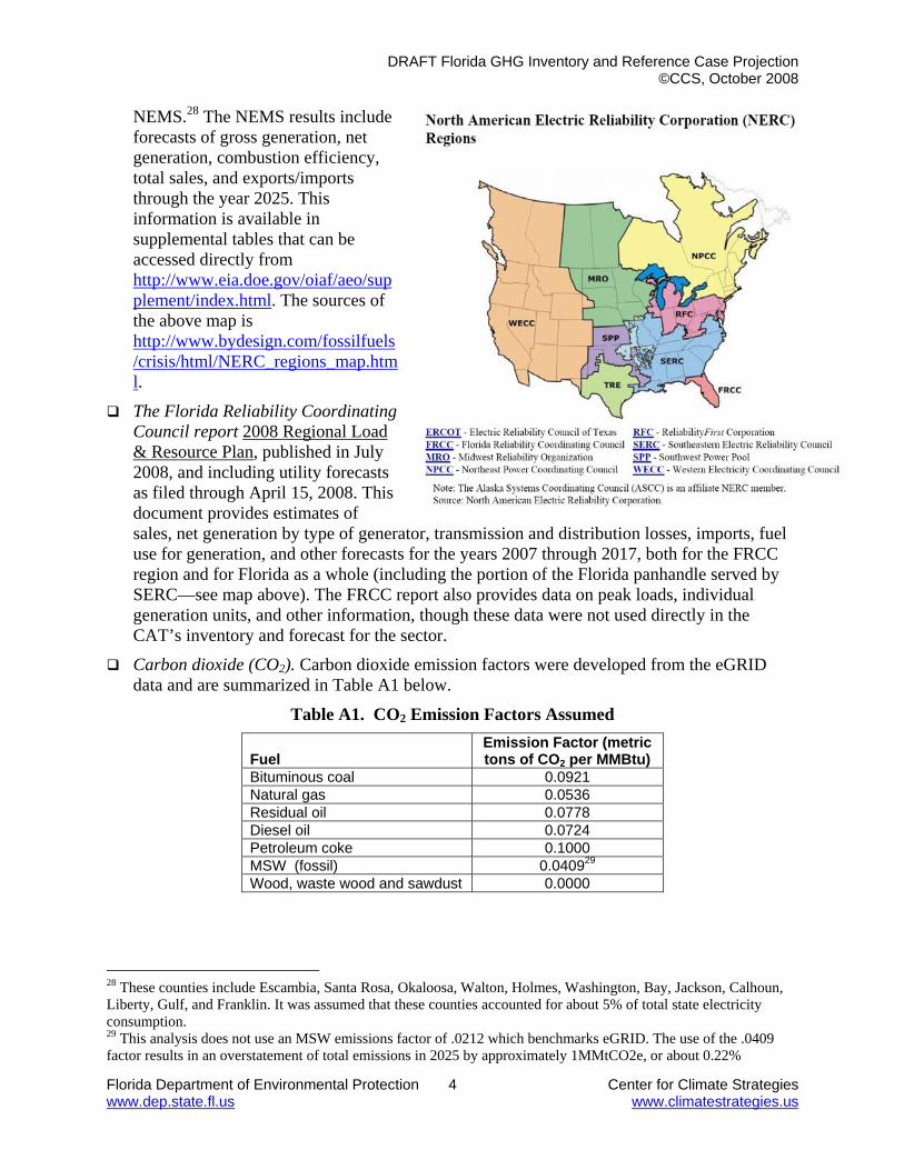
DRAFT Florida GHG Inventory and Reference Case Projection ©CCS, October 2008
Florida Department of Environmental Protection 4 Center for Climate Strategies www.dep.state.fl.us www.climatestrategies.us
NEMS.28 The NEMS results include forecasts of gross generation, net generation, combustion efficiency, total sales, and exports/imports through the year 2025. This information is available in supplemental tables that can be accessed directly from http://www.eia.doe.gov/oiaf/aeo/supplement/index.html. The sources of the above map is http://www.bydesign.com/fossilfuels/crisis/html/NERC_regions_map.html.
The Florida Reliability Coordinating Council report 2008 Regional Load & Resource Plan, published in July 2008, and including utility forecasts as filed through April 15, 2008. This document provides estimates of sales, net generation by type of generator, transmission and distribution losses, imports, fuel use for generation, and other forecasts for the years 2007 through 2017, both for the FRCC region and for Florida as a whole (including the portion of the Florida panhandle served by SERC—see map above). The FRCC report also provides data on peak loads, individual generation units, and other information, though these data were not used directly in the CAT’s inventory and forecast for the sector.
Carbon dioxide (CO2). Carbon dioxide emission factors were developed from the eGRID data and are summarized in Table A1 below.
Table A1. CO2 Emission Factors Assumed
Fuel Emission Factor (metric tons of CO2 per MMBtu)
Bituminous coal 0.0921 Natural gas 0.0536 Residual oil 0.0778 Diesel oil 0.0724 Petroleum coke 0.1000 MSW (fossil) 0.040929 Wood, waste wood and sawdust 0.0000
28 These counties include Escambia, Santa Rosa, Okaloosa, Walton, Holmes, Washington, Bay, Jackson, Calhoun, Liberty, Gulf, and Franklin. It was assumed that these counties accounted for about 5% of total state electricity consumption. 29 This analysis does not use an MSW emissions factor of .0212 which benchmarks eGRID. The use of the .0409 factor results in an overstatement of total emissions in 2025 by approximately 1MMtCO2e, or about 0.22%

DRAFT Florida GHG Inventory and Reference Case Projection ©CCS, October 2008
Florida Department of Environmental Protection 5 Center for Climate Strategies www.dep.state.fl.us www.climatestrategies.us
Greenhouse Gas Inventory Methodology for the Period 1990-1999 The methodology used to develop the Florida inventory of GHG emissions associated with electricity production and consumption for the period 1990-2006 is based on methods developed by the IPCC and used by the USEPA in the development of the US GHG inventory. There are three fundamental premises of the GHG inventory developed for Florida, as briefly described below:
The GHG inventory should be estimated based on both the production and consumption of electricity. Developing the production estimate involves tallying up the GHG emissions associated with the operation of power plants physically located in Florida, regardless of ownership. Developing the consumption estimate involves tallying up the GHG emissions associated with consumption of electricity in Florida, regardless of where the electricity is produced. As Florida is a net importer of electricity in most of the years, these estimates will be different.
The GHG inventory should be estimated based on emissions at the point of electric generation only. That is, GHG emissions associated with upstream fuel cycle process such as primary fuel extraction, transport to refinery/processing stations, refining, beneficiation, and transport to the power station are not included.
As an approximation, it was assumed that all power generated in Florida was consumed in Florida. In fact, some of the power generated in Florida is exported. However, given the similarity in the average carbon intensity of Florida power stations and that of power stations in the surrounding SERC region, the potential error associated with this simplifying assumption is likely to be small.
There were several steps in the methodology for the development of the electric sector GHG inventory for the period 1990-1999. These are briefly outlined below:
Determine the coal quality used in Florida power stations (i.e., share of anthracite, bituminous, lignite, sub-bituminous, and coal wastes used).
Determine gross annual primary energy consumption by Florida power stations by plant and fuel type.
Determine gross annual generation associated with net power imports to satisfy Florida electricity demand.
Multiply gross annual primary energy consumption by Florida power stations by CO2e emission factors. This provides an estimate of the Florida GHG inventory on a production basis.
Multiply annual gross generation associated with net power imports by the weighted average carbon emission intensity (in units of metric tons of CO2e per megawatt-hour [CO2e/MWh]) of the SERC region. This provides an estimate of the additional GHG emissions associated with meeting Florida electricity demand in excess of generation from local power plants.
Add the emissions associated with net power imports to the production-based emissions. This provides an estimate of the GHG inventory on a consumption basis.

DRAFT Florida GHG Inventory and Reference Case Projection ©CCS, October 2008
Florida Department of Environmental Protection 6 Center for Climate Strategies www.dep.state.fl.us www.climatestrategies.us
Greenhouse Gas Inventory Methodology for the Year 2000 The GHG inventory for 2000 associated with electric power production in Florida relies on the eGRID values. Annex A provides a detailed accounting of unit-level power plant and cogenerator CO2 emissions for the year 2000.
Greenhouse Gas Inventory Methodology for the Years 2001-2006 For the years 2001 through 2006, heat rates interpolated based on 2000 electricity generation fuel use data from the sources above and 2007 fuel use data from FRCC were used to estimate fuel used in generation from data on generation by fuel type. Estimates on fuel use were multiplied by the emission factors in Table A1, as applicable, to estimate CO2 emissions. A similar procedure was used to estimate other types of GHG emissions, using constant emission factors for CH4 and N2O.
Greenhouse Gas Inventory Results The results of the GHG inventory are summarized in Table A2 for the years 1990 and 2000, disaggregated by power producer type.
Table A2. GHG Inventory Results, Production-Based, 1990 and 2000 a) Year 1990
Fuel
Utilities and Cogenerators MMtCO2e
Generation (GWh)
Energy Use
(trillion Btu)
Heat Rate (Btu/kWh) Utilities Cogenerators Total
Coal 60,543 584 9,651 53.11 0.97 54.07Natural Gas 18,774 206 10,972 10.43 0.63 11.06Petroleum 25,723 260 10,110 19.90 0.38 20.28Nuclear 21,943 232 10,582 0.00 0.00 0.00 Hydroelectric 176 2 10,320 0.00 0.00 0.00 Solar/PV 1 0 10,320 0.00 0.00 0.00 MSW Landfill Gas 1,648 17 10,500 0.33 0.04 0.37 Biomass 2,181 23 10,500 0.00 0.01 0.02 Other wastes 1,453 15 10,500 0.00 0.34 0.34 Total 132,442 1,340 10,117 83.77 2.37 86.14
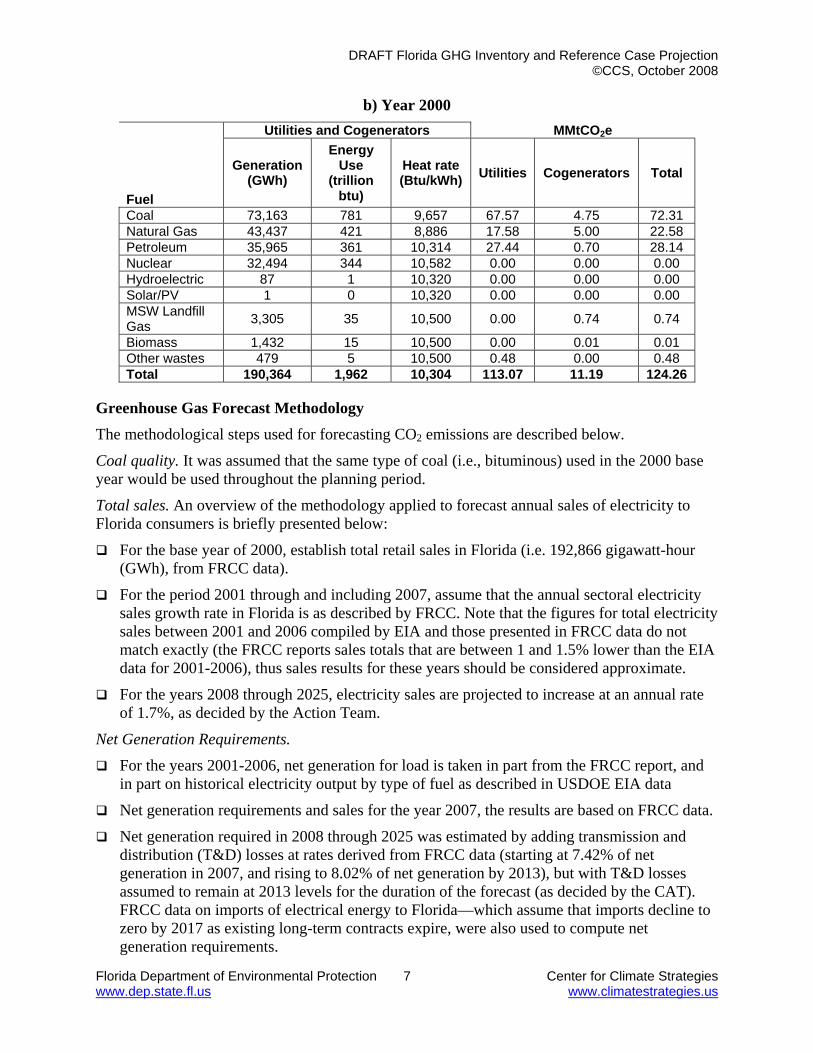
DRAFT Florida GHG Inventory and Reference Case Projection ©CCS, October 2008
Florida Department of Environmental Protection 7 Center for Climate Strategies www.dep.state.fl.us www.climatestrategies.us
b) Year 2000
Fuel
Utilities and Cogenerators MMtCO2e
Generation (GWh)
Energy Use
(trillion btu)
Heat rate (Btu/kWh) Utilities Cogenerators Total
Coal 73,163 781 9,657 67.57 4.75 72.31 Natural Gas 43,437 421 8,886 17.58 5.00 22.58 Petroleum 35,965 361 10,314 27.44 0.70 28.14 Nuclear 32,494 344 10,582 0.00 0.00 0.00 Hydroelectric 87 1 10,320 0.00 0.00 0.00 Solar/PV 1 0 10,320 0.00 0.00 0.00 MSW Landfill Gas 3,305 35 10,500 0.00 0.74 0.74
Biomass 1,432 15 10,500 0.00 0.01 0.01 Other wastes 479 5 10,500 0.48 0.00 0.48 Total 190,364 1,962 10,304 113.07 11.19 124.26
Greenhouse Gas Forecast Methodology The methodological steps used for forecasting CO2 emissions are described below.
Coal quality. It was assumed that the same type of coal (i.e., bituminous) used in the 2000 base year would be used throughout the planning period.
Total sales. An overview of the methodology applied to forecast annual sales of electricity to Florida consumers is briefly presented below:
For the base year of 2000, establish total retail sales in Florida (i.e. 192,866 gigawatt-hour (GWh), from FRCC data).
For the period 2001 through and including 2007, assume that the annual sectoral electricity sales growth rate in Florida is as described by FRCC. Note that the figures for total electricity sales between 2001 and 2006 compiled by EIA and those presented in FRCC data do not match exactly (the FRCC reports sales totals that are between 1 and 1.5% lower than the EIA data for 2001-2006), thus sales results for these years should be considered approximate.
For the years 2008 through 2025, electricity sales are projected to increase at an annual rate of 1.7%, as decided by the Action Team.
Net Generation Requirements.
For the years 2001-2006, net generation for load is taken in part from the FRCC report, and in part on historical electricity output by type of fuel as described in USDOE EIA data
Net generation requirements and sales for the year 2007, the results are based on FRCC data.
Net generation required in 2008 through 2025 was estimated by adding transmission and distribution (T&D) losses at rates derived from FRCC data (starting at 7.42% of net generation in 2007, and rising to 8.02% of net generation by 2013), but with T&D losses assumed to remain at 2013 levels for the duration of the forecast (as decided by the CAT). FRCC data on imports of electrical energy to Florida—which assume that imports decline to zero by 2017 as existing long-term contracts expire, were also used to compute net generation requirements.

DRAFT Florida GHG Inventory and Reference Case Projection ©CCS, October 2008
Florida Department of Environmental Protection 8 Center for Climate Strategies www.dep.state.fl.us www.climatestrategies.us
Electricity Output by Fuel.
FRCC data for electricity output by fuel were used to estimate output by fuel in the years 2008 through 2017 except that, at the direction of the Action Team: 1) Generation from solar photovoltaic/solar thermal power plants expected to come on line between 2010 and 2011 was added to the generation mix; and 2) Natural gas generation in each year after 2008 was reduced to meet requirements for net generation.
For the years 2018 through 2025, the CAT forecast period after the FRCC forecast ends, FRCC trends for generation share for coal, petroleum, and renewables generation for the years 2012 through 2017 were used to extrapolate estimates of generation by those fuels. The same approach was used to extrapolate nuclear generation through 2022, after which nuclear output was assumed, based on Action Team input, to remain at just under 67 TWh/yr for the duration of the forecast
Natural gas generation in 2018 through 2025 was adjusted to meet total net generation requirements.
Net and Gross generation. An overview of the methodology applied to forecast annual gross electricity generation by Florida power stations is briefly summarized below:
For 2000 through 2025, assume losses associated with on-site usage of electricity by plant type for Florida power plants are equal to the average for the NERC region in which Florida is located, based on Annual Energy Outlook data (0.74% of net generation in 2000, falling to 0.44% of net generation in 2025).
For the base year of 2000, combine actual net electric generation data and estimated on-site losses to estimate gross generation by plant type.
Combustion efficiency. An overview of the methodology applied to forecast annual heat rates at Florida power stations is briefly summarized below:
For the 2000, estimate gross heat rate of Florida power stations by dividing the plant type-specific gross primary energy consumption by the plant type-specific gross generation.
For the period 2001 through 2006, interpolate between year 2000 heat rates as derived above and 2007 heat rates as determined from FRCC data.
For the period 2007 through 2017, heat rates as implied in FRCC fuel use forecasts were applied to net generation estimates prepared as above.
Throughout the period 2018 through 2025, 2017 heat rates derived from the FRCC forecast were assumed to apply.
Energy use. An overview of the methodology applied to forecast annual primary energy use at Florida power stations is briefly summarized below:
For the base year of 2000, primary rely on the eGRID results.
For the period 2001 through and including 2025, multiply annual gross generation by annual heat rate for each plant type in Florida, using combustion efficiencies derived as above.
Gross generation associated with electricity exports/imports. An overview of the methodology applied to forecast annual gross generation associated with electricity imports to Florida is briefly summarized below:

DRAFT Florida GHG Inventory and Reference Case Projection ©CCS, October 2008
Florida Department of Environmental Protection 9 Center for Climate Strategies www.dep.state.fl.us www.climatestrategies.us
For the base year of 2000 through and including 2025, all imported electricity is assumed to come from the SERC region.
For the base year of 2000 through and including 2025, if the total gross generation at FL power stations is less than the total gross generation required to meet demand, it is assumed that this difference is imported from the SERC region.
Primary energy associated with electricity imports. An overview of the methodology applied to forecast annual primary energy associated with electricity imports to Florida is briefly summarized below:
For the base year of 2000 through and including 2025, if the total primary energy consumed at Florida power stations is less than the total primary energy required to meet demand, it is assumed that the difference is imported from the SERC NERC region in the form of electricity.
Carbon dioxide-equivalent emissions from Florida power stations. An overview of the methodology applied to forecast annual CO2e emissions from Florida power stations is briefly summarized below:
For the base year of 2000 through and including 2025, estimate total CO2 emissions from Florida power stations by multiplying total primary energy use by the CO2 emission factor and the global warming potential.
For the base year of 2000 through and including 2025, estimate total CH4 emissions from Florida power stations by multiplying total primary energy use by the CH4 emission factor and the global warming potential.
For the base year of 2000 through and including 2025, estimate total N2O emissions from Florida power stations by multiplying total primary energy use by the N2O emission factor and the global warming potential.
For the base year of 2000 through and including 2025, estimate total CO2e emissions from Florida power stations by adding the CO2e of CO2, CH4, and N2O.
Carbon dioxide-equivalent emissions from imported electricity. An overview of the methodology applied to forecast annual CO2e emissions from electricity imports is briefly summarized below:
For the base year of 2000 through and including 2025, estimate total CO2 emissions associated with imports by multiplying total primary energy use associated with imports by the CO2 emission factor and its global warming potential.
For the base year of 2000 through and including 2025, estimate total CH4 emissions associated with imports by multiplying total primary energy use associated with imports by the CH4 emission factor and its global warming potential.
For the base year of 2000 through and including 2025, estimate total N2O emissions associated with imports by multiplying total primary energy use associated with imports by the N2O emission factor and its global warming potential.
For the base year of 2000 through and including 2025, estimate total CO2e emissions associated with imported electricity by adding the CO2e of CO2, CH4, and N2O.
Greenhouse Gas Forecast Results

DRAFT Florida GHG Inventory and Reference Case Projection ©CCS, October 2008
Florida Department of Environmental Protection 10 Center for Climate Strategies www.dep.state.fl.us www.climatestrategies.us
This section provides an overview of the results of the GHG emissions inventory and reference case projections estimated using the methodological approach described above. Table A3 and Figure A1 summarize the characteristics of the electric generation system forecast for Florida. Total primary energy consumption associated with electricity generation in Florida is summarized in Figure A2 and in Table A4. Total gross generation by Florida power plants is summarized in Figure A3 and in Table A5. Total GHG emissions associated with electricity generation to meet electricity demand within Florida are summarized in Figure A4 and in Table A6 by fuel type.
On a consumption basis, emissions were about 101 MMtCO2e in 1990, increased to 136 MMtCO2e in 2000 and are projected to increase to about 158 MMtCO2e in 2025. This represents a 35% increase in emissions associated with Florida’s electricity demand from 1990 to 2000 and a 16% increase from 2000 to 2025. Florida has been a net importer of electricity and is projected to continue to be a net importer through at least 2016. Hence, GHG emissions will likely continue to be higher on a consumption basis than on a production basis. Emissions associated with imported electricity vary depending on the supply of electricity available from out-of-state generators.
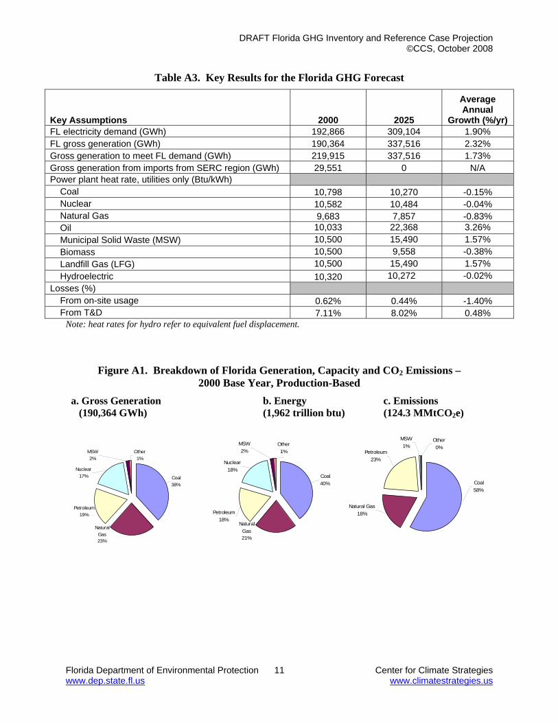
DRAFT Florida GHG Inventory and Reference Case Projection ©CCS, October 2008
Florida Department of Environmental Protection 11 Center for Climate Strategies www.dep.state.fl.us www.climatestrategies.us
Table A3. Key Results for the Florida GHG Forecast
Key Assumptions 2000 2025
Average Annual
Growth (%/yr) FL electricity demand (GWh) 192,866 309,104 1.90% FL gross generation (GWh) 190,364 337,516 2.32% Gross generation to meet FL demand (GWh) 219,915 337,516 1.73% Gross generation from imports from SERC region (GWh) 29,551 0 N/A Power plant heat rate, utilities only (Btu/kWh) Coal 10,798 10,270 -0.15% Nuclear 10,582 10,484 -0.04% Natural Gas 9,683 7,857 -0.83% Oil 10,033 22,368 3.26% Municipal Solid Waste (MSW) 10,500 15,490 1.57% Biomass 10,500 9,558 -0.38% Landfill Gas (LFG) 10,500 15,490 1.57% Hydroelectric 10,320 10,272 -0.02% Losses (%) From on-site usage 0.62% 0.44% -1.40% From T&D 7.11% 8.02% 0.48%
Note: heat rates for hydro refer to equivalent fuel displacement.
Figure A1. Breakdown of Florida Generation, Capacity and CO2 Emissions – 2000 Base Year, Production-Based
a. Gross Generation b. Energy c. Emissions (190,364 GWh) (1,962 trillion btu) (124.3 MMtCO2e)
Coal38%
Natural Gas23%
Petroleum19%
Nuclear17%
Other1%
MSW2%
MSW2%
Other1%
Nuclear18%
Petroleum18%
Natural Gas21%
Coal40%
Coal58%
Natural Gas18%
Petroleum23%
MSW1%
Other0%
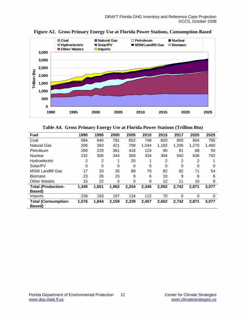
DRAFT Florida GHG Inventory and Reference Case Projection ©CCS, October 2008
Florida Department of Environmental Protection 12 Center for Climate Strategies www.dep.state.fl.us www.climatestrategies.us
Figure A2. Gross Primary Energy Use at Florida Power Stations, Consumption-Based
0
500
1,000
1,500
2,000
2,500
3,000
3,500
1990 1995 2000 2005 2010 2015 2020 2025
Trill
ion
Btu
Coal Natural Gas Petroleum NuclearHydroelectric Solar/PV MSW Landfill Gas BiomassOther Wastes Imports
Table A4. Gross Primary Energy Use at Florida Power Stations (Trillion Btu) Fuel 1990 1995 2000 2005 2010 2015 2017 2020 2025Coal 584 640 781 652 748 820 800 804 795Natural Gas 206 393 421 708 1,044 1,182 1,206 1,270 1,460Petroleum 260 229 361 418 124 90 81 68 50Nuclear 232 306 344 309 334 394 550 638 702Hydroelectric 2 2 1 20 1 2 2 2 1Solar/PV 0 0 0 0 0 0 0 0 0MSW Landfill Gas 17 33 35 88 79 82 82 71 54Biomass 23 26 15 9 6 10 9 8 6Other Wastes 15 22 5 0 8 12 11 10 8Total (Production-Based)
1,340 1,651 1,962 2,204 2,345 2,592 2,742 2,871 3,077
Imports 236 193 197 134 112 70 0 0 0Total (Consumption-Based)
1,576 1,844 2,159 2,339 2,457 2,662 2,742 2,871 3,077
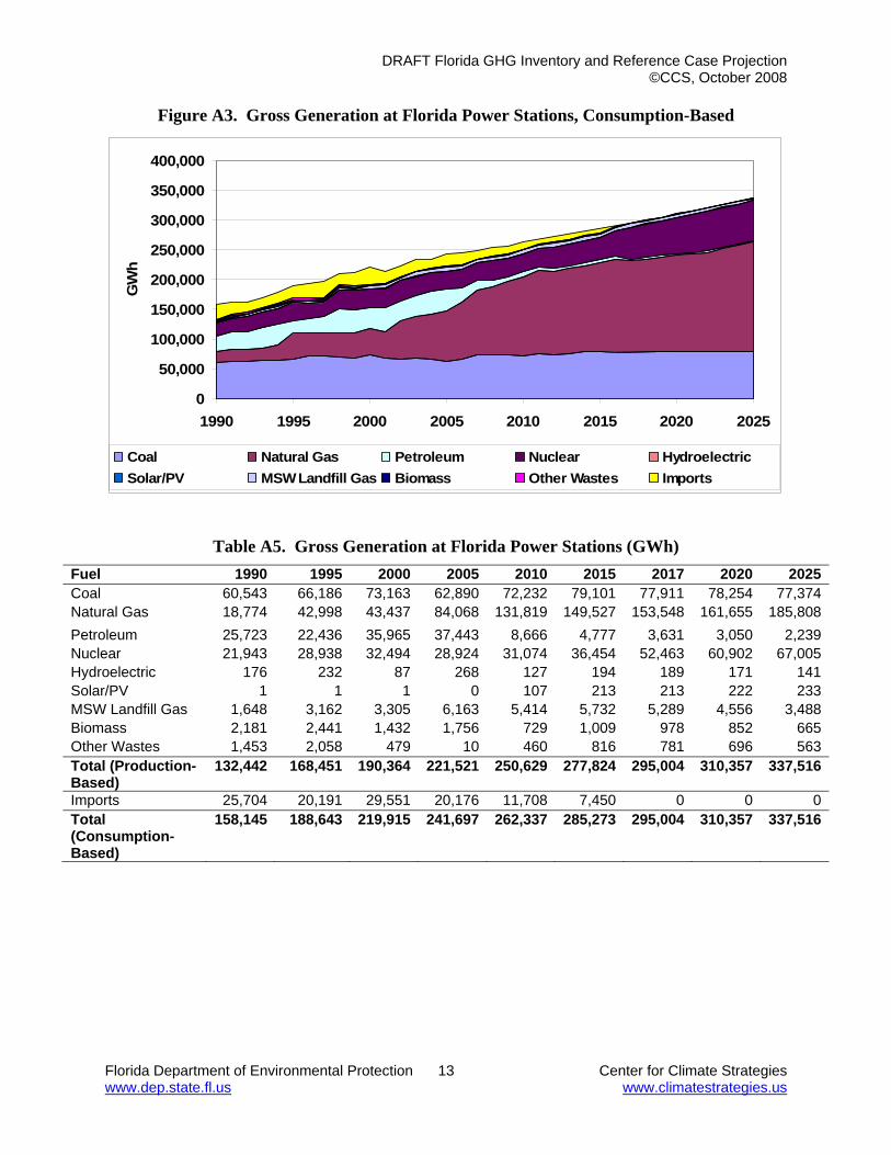
DRAFT Florida GHG Inventory and Reference Case Projection ©CCS, October 2008
Florida Department of Environmental Protection 13 Center for Climate Strategies www.dep.state.fl.us www.climatestrategies.us
Figure A3. Gross Generation at Florida Power Stations, Consumption-Based
0
50,000
100,000
150,000
200,000
250,000
300,000
350,000
400,000
1990 1995 2000 2005 2010 2015 2020 2025
GW
h
Coal Natural Gas Petroleum Nuclear HydroelectricSolar/PV MSW Landfill Gas Biomass Other Wastes Imports
Table A5. Gross Generation at Florida Power Stations (GWh) Fuel 1990 1995 2000 2005 2010 2015 2017 2020 2025Coal 60,543 66,186 73,163 62,890 72,232 79,101 77,911 78,254 77,374Natural Gas 18,774 42,998 43,437 84,068 131,819 149,527 153,548 161,655 185,808Petroleum 25,723 22,436 35,965 37,443 8,666 4,777 3,631 3,050 2,239Nuclear 21,943 28,938 32,494 28,924 31,074 36,454 52,463 60,902 67,005Hydroelectric 176 232 87 268 127 194 189 171 141Solar/PV 1 1 1 0 107 213 213 222 233MSW Landfill Gas 1,648 3,162 3,305 6,163 5,414 5,732 5,289 4,556 3,488Biomass 2,181 2,441 1,432 1,756 729 1,009 978 852 665Other Wastes 1,453 2,058 479 10 460 816 781 696 563Total (Production-Based)
132,442 168,451 190,364 221,521 250,629 277,824 295,004 310,357 337,516
Imports 25,704 20,191 29,551 20,176 11,708 7,450 0 0 0Total (Consumption-Based)
158,145 188,643 219,915 241,697 262,337 285,273 295,004 310,357 337,516
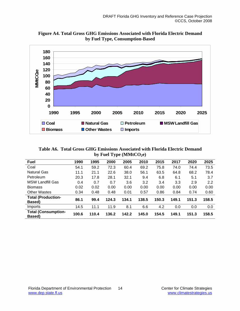
DRAFT Florida GHG Inventory and Reference Case Projection ©CCS, October 2008
Florida Department of Environmental Protection 14 Center for Climate Strategies www.dep.state.fl.us www.climatestrategies.us
Figure A4. Total Gross GHG Emissions Associated with Florida Electric Demand by Fuel Type, Consumption-Based
020406080
100120140160180
1990 1995 2000 2005 2010 2015 2020 2025
MM
tCO 2
e
Coal Natural Gas Petroleum MSW Landfill GasBiomass Other Wastes Imports
Table A6. Total Gross GHG Emissions Associated with Florida Electric Demand by Fuel Type (MMtCO2e)
Fuel 1990 1995 2000 2005 2010 2015 2017 2020 2025Coal 54.1 59.2 72.3 60.4 69.2 75.8 74.0 74.4 73.5Natural Gas 11.1 21.1 22.6 38.0 56.1 63.5 64.8 68.2 78.4Petroleum 20.3 17.8 28.1 32.1 9.4 6.8 6.1 5.1 3.7MSW Landfill Gas 0.4 0.7 0.7 3.6 3.2 3.4 3.3 2.9 2.2Biomass 0.02 0.02 0.00 0.00 0.00 0.00 0.00 0.00 0.00Other Wastes 0.34 0.48 0.48 0.01 0.57 0.86 0.84 0.74 0.60Total (Production-Based) 86.1 99.4 124.3 134.1 138.5 150.3 149.1 151.3 158.5
Imports 14.5 11.1 11.9 8.1 6.6 4.2 0.0 0.0 0.0Total (Consumption-Based) 100.6 110.4 136.2 142.2 145.0 154.5 149.1 151.3 158.5

DRAFT Florida GHG Inventory and Reference Case Projection ©CCS, October 2008
Florida Department of Environmental Protection 15 Center for Climate Strategies www.dep.state.fl.us www.climatestrategies.us
Key Uncertainties Key sources of uncertainty underlying the estimates above are as follows:
• The forecast relies primarily on FRCC data for changes in generation fractions for coal- and oil-fired power, especially through 2017. As such, it depends on estimates of future generating capacity and generation by Florida utilities. In addition, an assumed growth rate of 1.7% per year underlies all sales estimates from 2008 through 2025, and thus all of the forecast estimates. Although this estimate was deemed consistent with recent trends in Florida by the Action Team and others, it may well vary over time.
• Average electricity on-site usage and transmission and distribution loss estimates were used to estimate gross generation requirements based on the electricity sales forecast. The on-site usage and transmission and distribution loss estimates are taken from the FRCC values for 2007 through 2013, and assumed to be constant from 2013 on. Changes in the Florida electricity grid, including investments to improve grid performance and/or changes in peak loadings (for example), could result in actual values that are different from these estimates.
• The origin of electricity imported to Florida has been assumed to be the SERC region. If in fact, some imported power comes from the SPP or other regions, this would have impact on the carbon intensity of electricity imports. Improvements to these estimates (based on unit-specific input) could help to get more accurate emissions associated with imported electricity, as could a better estimates of the likely status of imports in the future (particularly in the period when existing import contracts begin to lapse).
• There are uncertainties associated with the statewide fuel mix, emission factors, and conversion factors (to convert electricity from a heat input basis to electricity output) that should be reviewed and revised with data that is specific to Florida power generators.
• Fuel price changes influence consumption levels and, to the extent that price trends for competing fuels differ, may encourage switching among fuels, and thereby affect emissions estimates. Unanticipated events that affect fuel prices could affect the electricity forecast for Florida.

DRAFT Florida GHG Inventory and Reference Case Projection ©CCS, June 2008
Florida Department of Environmental Protection 16 Center for Climate Strategies www.dep.state.fl.us www.climatestrategies.us
Annex A – eGRID CO2 Emissions for the Year 2000
Facility ID
Federal ID OWNER/COMPANY NAME SITE NAME
CO2 Emissions Energy Use Metric
Tons Short Tons MMBtu Total 123,747,763 136,286,083 1,616,501,572 1070025 136 SEMINOLE ELECTRIC COOPERATIVE, INC. SEMINOLE GENERATING STATION 9,465,290 10,424,329 101,601,605 0870020 164 KEYS ENERGY SERVICES BIG PINE KEY 1,337 1,473 18,451 0310045 207 JEA SJRPP 9,815,184 10,809,674 105,372,831 0950137 564 ORLANDO UTILITIES COMMISSION STANTON ENERGY CENTER 5,967,537 6,572,178 65,284,719 0090006 609 FLORIDA POWER & LIGHT (PCC) CAPE CANAVERAL PLANT 2,437,960 2,684,978 33,404,537 0250001 610 FLORIDA POWER & LIGHT (PCU) CUTLER POWER PLANT 242,178 266,715 4,487,996 0710002 612 FLORIDA POWER & LIGHT (PFM) FORT MYERS POWER PLANT 2,209,976 2,433,894 27,471,081 0110037 613 FLORIDA POWER & LIGHT (PFL) FT. LAUDERDALE POWER PLANT 2,664,980 2,935,000 49,387,556 0110036 617 FLORIDA POWER & LIGHT (PPE) PORT EVERGLADES POWER PLANT 3,932,563 4,331,017 52,832,377 0990042 619 FLORIDA POWER & LIGHT (PRV) RIVIERA POWER PLANT 1,880,746 2,071,307 24,413,567 1270009 620 FLORIDA POWER & LIGHT (PSN) SANFORD POWER PLANT 2,686,696 2,958,916 35,630,263 0250003 621 FLORIDA POWER & LIGHT (PTF) TURKEY POINT POWER PLANT 2,463,181 2,712,755 33,911,100 0550003 624 FLORIDA POWER CORPORATION D/B/A PROGRESS AVON PARK 30,674 33,782 526,079 1030013 627 FLORIDA POWER CORPDBAPROGRESS ENERGY FLA BAYBORO POWER PLANT 123,282 135,773 1,700,839 0170004 628 FLORIDA POWER CORPORATION D/B/A PROGRESS CRYSTAL RIVER POWER PLANT 14,013,373 15,433,230 150,421,371 1270020 629 FLORIDA POWER CORPORATION D/B/A PROGRESS TURNER PLANT 55,917 61,583 771,455 1030012 630 FLORIDA POWER CORPDBAPROGRESS ENERGY FLA HIGGINS PLANT 75,390 83,029 1,418,457 1030011 634 FLORIDA POWER CORPDBAPROGRESS ENERGY FLA BARTOW PLANT 1,614,458 1,778,037 22,343,040 0950014 637 FLORIDA POWER CORPORATION D/B/A PROGRESS RIO PINAR PEAKING FACILITY 3,712 4,088 51,209 1210003 638 FLORIDA POWER CORPDBAPROGRESS ENERGY FLA FL POWER SUWANNEE RVR PLANT 420,197 462,772 5,374,922 0330045 641 GULF POWER COMPANY CRIST ELECTRIC GENERATING PLANT 5,863,225 6,457,296 63,804,948 0630014 642 GULF POWER COMPANY SCHOLZ ELECTRIC GENERATING PLANT 416,374 458,562 4,469,397 0050014 643 GULF POWER COMPANY LANSING SMITH PLANT 2,597,038 2,860,174 27,914,913 0570039 645 TAMPA ELECTRIC COMPANY BIG BEND STATION 10,539,299 11,607,158 113,434,399
0570040 646 TAMPA ELECTRIC COMPANY F.J. GANNON STATION 4,847,299 5,338,435 52,038,375
0570038 647 TAMPA ELECTRIC COMPANY HOOKERS POINT STATION 222,560 245,110 3,028,473
1110003 658 FT PIERCE UTILITIES AUTHORITY FT PIERCE UTIL/H D KING PWR PLNT 66,748 73,511 1,241,544
0010006 663 CITY OF GAINESVILLE, GRU DEERHAVEN GENERATING STATION 1,722,338 1,896,848 19,953,930
0010005 664 GAINESVILLE REGIONAL UTILITIES JOHN R KELLY POWER PLANT 56,422 62,138 1,025,001
0250013 665 HOMESTEAD CITY UTILITIES GORDON W. IVEY POWER PLANT 46,985 51,745 803,064
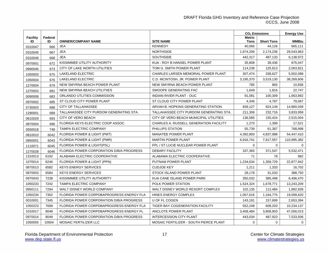
DRAFT Florida GHG Inventory and Reference Case Projection ©CCS, June 2008
Florida Department of Environmental Protection 17 Center for Climate Strategies www.dep.state.fl.us www.climatestrategies.us
Facility ID
Federal ID OWNER/COMPANY NAME SITE NAME
CO2 Emissions Energy Use Metric
Tons Short Tons MMBtu 0310047 666 JEA KENNEDY 40,066 44,126 665,111
0310045 667 JEA NORTHSIDE 1,974,206 2,174,236 29,543,963
0310046 668 JEA SOUTHSIDE 442,317 487,133 6,138,972
0970001 672 KISSIMMEE UTILITY AUTHORITY KUA - ROY B HANSEL POWER PLANT 35,808 39,436 675,047
0990045 673 CITY OF LAKE WORTH UTILITIES TOM G. SMITH POWER PLANT 114,238 125,813 2,063,821
1050003 675 LAKELAND ELECTRIC CHARLES LARSEN MEMORIAL POWER PLANT 307,474 338,627 5,502,088
1050004 676 LAKELAND ELECTRIC C.D. MCINTOSH, JR. POWER PLANT 3,195,370 3,519,130 38,269,606
1270004 679 NEW SMYRNA BEACH POWER PLANT NEW SMYRNA BEACH POWER PLANT 785 865 10,836
1270003 681 NEW SMYRNA BEACH UTILITIIES SWOOPE GENERATING FAC 1,649 1,816 22,747
0090008 683 ORLANDO UTLITIES COMMISSION INDIAN RIVER PLANT - OUC 91,081 100,309 1,663,892
0970002 685 ST CLOUD CITY POWER PLANT ST CLOUD CITY POWER PLANT 4,346 4,787 79,067
0730003 688 CITY OF TALLAHASSEE ARVAH B. HOPKINS GENERATING STATION 839,127 924,149 14,860,039
1290001 689 TALLAHASSEE CITY PURDOM GENERATING STA. TALLAHASSEE CITY PURDOM GENERATING STA. 211,306 232,716 3,833,958
0610029 693 CITY OF VERO BEACH CITY OF VERO BEACH MUNICIPAL UTILITIES 136,585 150,424 2,515,004
0870004 696 FLORIDA KEYS ELECTRIC COOP ASSOC CHARLES A. RUSSELL GENERATION FACILITY 1,270 1,399 17,521
0550018 748 TAMPA ELECTRIC COMPANY PHILLIPS STATION 55,739 61,387 768,998
0810010 6042 FLORIDA POWER & LIGHT (PMT) MANATEE POWER PLANT 4,392,893 4,837,988 54,447,410
0850001 6043 FLORIDA POWER & LIGHT (PMR) MARTIN POWER PLANT 6,916,741 7,617,557 110,995,382
1110071 6045 FLORIDA POWER & LIGHT(PSL) FPL / ST LUCIE NUCLEAR POWER PLANT 0 0 0
1270028 6046 FLORIDA POWER CORPORATION D/B/A PROGRESS DEBARY FACILITY 337,365 371,547 5,532,471 1310013 6192 ALABAMA ELECTRIC COOPERATIVE ALABAMA ELECTRIC COOPERATIVE 71 78 982 1070014 6246 FLORIDA POWER & LIGHT (PPN) PUTNAM POWER PLANT 1,234,634 1,359,729 22,877,942 0870013 6582 KEYS ENERGY SERVICES CUDJOE KEY 1,211 1,333 16,702 0870003 6584 KEYS ENERGY SERVICES STOCK ISLAND POWER PLANT 28,178 31,033 388,750 0970043 7238 KISSIMMEE UTILITY AUTHORITY KUA CANE ISLAND POWER PARK 350,032 385,498 6,496,470 1050233 7242 TAMPA ELECTRIC COMPANY POLK POWER STATION 1,524,324 1,678,771 13,243,209 0950111 7294 WALT DISNEY WORLD COMPANY WALT DISNEY WORLD RESORT COMPLEX 102,135 112,484 1,892,939 1050234 7302 FLORIDA POWER CORPDBAPROGRESS ENERGY FLA HINES ENERGY COMPLEX 1,057,616 1,164,775 19,599,620 0010001 7345 FLORIDA POWER CORPORATION D/B/A PROGRESS U OF FL COGEN 143,191 157,699 2,653,394 1050223 7699 FLORIDA POWER CORPDBAPROGRESS ENERGY FLA TIGER BAY COGENERATION FACILITY 552,248 608,203 10,234,137 1010017 8048 FLORIDA POWER CORPDBAPROGRESS ENERGY FL ANCLOTE POWER PLANT 3,458,484 3,808,903 47,056,013 0970014 8049 FLORIDA POWER CORPORATION D/B/A PROGRESS INTERCESSION CITY PLANT 443,034 487,923 7,533,506 1050055 10004 MOSAIC FERTILIZER LLC MOSAIC FERTILIZER - SOUTH PIERCE PLANT 0 0 0

DRAFT Florida GHG Inventory and Reference Case Projection ©CCS, June 2008
Florida Department of Environmental Protection 18 Center for Climate Strategies www.dep.state.fl.us www.climatestrategies.us
Facility ID
Federal ID OWNER/COMPANY NAME SITE NAME
CO2 Emissions Energy Use Metric
Tons Short Tons MMBtu 0310010 10008 BAPTIST MEDICAL CENTER BAPTIST MEDICAL CENTER 43,942 48,394 835,116 0690002 10020 CUTRALE CITRUS JUICES USA INC CUTRALE CITRUS JUICES USA - LEESBURG 12,725 14,014 242,042 0250348 10062 MIAMI DADE RRF MIAMI DADE RRF/MONTENAY 69,655 76,713 2,950,521 1050023 10188 CUTRALE CITRUS JUICES USA,INC CUTRALE CITRUS JUICES USA,INC 22,443 24,717 426,903 0890003 10202 SMURFIT-STONE CONTAINER ENTERPRISES, INC FERNANDINA BEACH MILL 70,195 77,307 4,862,020 0570008 10204 MOSAIC FERTILIZER, LLC MOSAIC FERTILIZER-RIVERVIEW FACILITY 3,998 4,404 3,689,611 1050053 10205 MOSAIC FERTILIZER, LLC MOSAIC FERTILIZER - GREEN BAY FACILITY 0 0 1,889,796 0050031 10250 BAY COUNTY BOARD OF COUNTY COMMISSIONERS MONTENAY BAY, LLC 36,489 40,186 1,556,415 1050106 10275 CITRUS WORLD, INC. FLORIDA'S NATURAL GROWERS--BARTOW 15,533 17,107 295,466 0530021 10333 FLORIDA CRUSHED STONE CO., INC. BROOKSVILLE CEMENT AND POWER PLANTS 934,909 1,029,635 9,997,286 0650001 10347 SI GROUP-ENERGY, LLC MONTICELLO PLANT 0 0 174,000 0330040 10416 SOLUTIA INC. SOLUTIA INC. 258,650 284,857 4,864,074 0310006 10431 ANHEUSER BUSCH, INC. JACKSONVILLE ANHEUSER BUSCH, INC. JACKSONVILLE 25,751 28,361 489,825 1050059 10434 MOSAIC FERTILIZER LLC MOSAIC FERTILIZER - NEW WALES PLANT 0 0 0 0890004 10562 RAYONIER PERFORMANCE FIBERS LLC FERNANDINA SULFITE MILL 6,949 7,653 1,708,799 1070005 10611 GEORGIA-PACIFIC CONSUMER OPERATIONS LLC PALATKA PULP & PAPER MILL 49,903 54,959 5,760,318 0310337 10672 CEDAR BAY GENERATING COMPANY, L.P. CEDAR BAY COGENERATION FACILITY 1,735,924 1,911,811 18,559,146 0990234 50071 SOLID WASTE AUTHORITY OF PBC SOLID WASTE AUTHORITY OF PBC/NCRRF 146,177 160,987 6,209,881 0330042 50250 INTERNATIONAL PAPER COMPANY PENSACOLA MILL 28,943 31,876 4,135,906 1050051 50291 U.S. AGRI-CHEMICALS CORPORATION U.S. AGRI-CHEMICALS - FT. MEADE 0 0 1,723,087 0330114 50310 PENSACOLA CHRISTIAN COLLEGE, INC. PENSACOLA CHRISTIAN COLLEGE, INC. 645 710 12,268 0570005 50371 CF INDUSTRIES, INC., PLANT CITY PHOS CF INDUSTRIES-PLANT CITY PHOSP COMPLEX 187 206 5,701,085 1230001 50466 BUCKEYE FLORIDA, LIMITED PARTNERSHIP BUCKEYE FLORIDA, LIMITED PARTNERSHIP 132 145 2,797,656 0470002 50473 WHITE SPRINGS AGRICULTURAL CHEMICALS,INC WHITE SPRS AG CHEM-SR/SC CMPLX 8,818 9,711 438,242 0470002 50474 WHITE SPRINGS AGRICULTURAL CHEMICALS,INC WHITE SPRS AG CHEM-SR/SC CMPLX 2,818 3,103 749,996 0510003 50482 U.S. SUGAR CORP. CLEWISTON MILL U.S. SUGAR CLEWISTON MILL AND REFINERY 68 75 960,339 0990061 50483 U.S.SUGAR CORP. BRYANT MILL U.S. SUGAR CORP. BRYANT MILL 5 6 590,358 0112094 50572 WASTE MANAGEMENT INC. OF FLORIDA CENTRAL DISPOSAL 1,864 2,053 1,090,403 0690046 50629 COVANTA LAKE II, INC. LAKE COUNTY RESOURCE RECOVERY FACILITY 34,294 37,769 1,465,200 1050046 50633 MOSAIC FERTILIZER, LLC MOSAIC FERTILIZER - BARTOW FACILITY 3,077 3,388 4,193,114
1010056 50666 PASCO COUNTY PASCO COUNTY RESOURCE RECOVERY FACILITY 36,736 40,458 1,566,139
1130014 50725 PETRO OPERATING COMPANY BLACKJACK CREEK 588 648 11,189 0770009 50774 CQ BIOPOWER PRODUCERS, LLC TELOGIA POWER, LLC 0 0 1,194,233
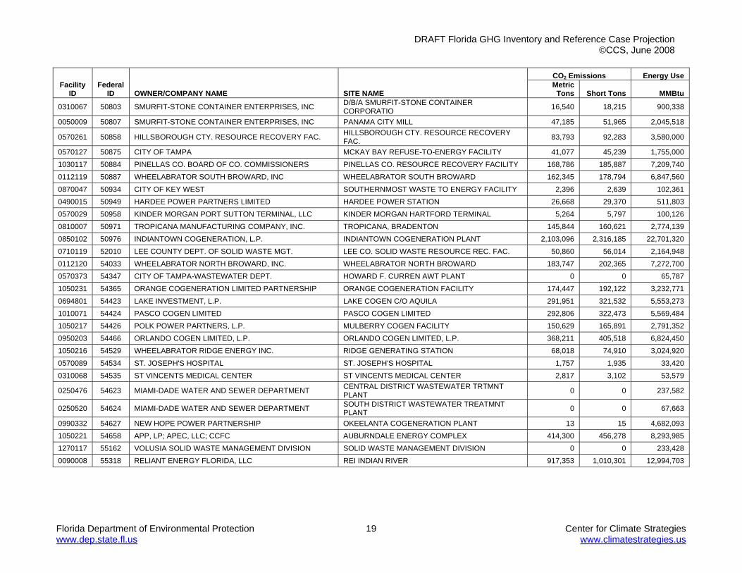
DRAFT Florida GHG Inventory and Reference Case Projection ©CCS, June 2008
Florida Department of Environmental Protection 19 Center for Climate Strategies www.dep.state.fl.us www.climatestrategies.us
Facility ID
Federal ID OWNER/COMPANY NAME SITE NAME
CO2 Emissions Energy Use Metric
Tons Short Tons MMBtu
0310067 50803 SMURFIT-STONE CONTAINER ENTERPRISES, INC D/B/A SMURFIT-STONE CONTAINER CORPORATIO 16,540 18,215 900,338
0050009 50807 SMURFIT-STONE CONTAINER ENTERPRISES, INC PANAMA CITY MILL 47,185 51,965 2,045,518
0570261 50858 HILLSBOROUGH CTY. RESOURCE RECOVERY FAC. HILLSBOROUGH CTY. RESOURCE RECOVERY FAC. 83,793 92,283 3,580,000
0570127 50875 CITY OF TAMPA MCKAY BAY REFUSE-TO-ENERGY FACILITY 41,077 45,239 1,755,000 1030117 50884 PINELLAS CO. BOARD OF CO. COMMISSIONERS PINELLAS CO. RESOURCE RECOVERY FACILITY 168,786 185,887 7,209,740 0112119 50887 WHEELABRATOR SOUTH BROWARD, INC WHEELABRATOR SOUTH BROWARD 162,345 178,794 6,847,560 0870047 50934 CITY OF KEY WEST SOUTHERNMOST WASTE TO ENERGY FACILITY 2,396 2,639 102,361 0490015 50949 HARDEE POWER PARTNERS LIMITED HARDEE POWER STATION 26,668 29,370 511,803 0570029 50958 KINDER MORGAN PORT SUTTON TERMINAL, LLC KINDER MORGAN HARTFORD TERMINAL 5,264 5,797 100,126 0810007 50971 TROPICANA MANUFACTURING COMPANY, INC. TROPICANA, BRADENTON 145,844 160,621 2,774,139 0850102 50976 INDIANTOWN COGENERATION, L.P. INDIANTOWN COGENERATION PLANT 2,103,096 2,316,185 22,701,320 0710119 52010 LEE COUNTY DEPT. OF SOLID WASTE MGT. LEE CO. SOLID WASTE RESOURCE REC. FAC. 50,860 56,014 2,164,948 0112120 54033 WHEELABRATOR NORTH BROWARD, INC. WHEELABRATOR NORTH BROWARD 183,747 202,365 7,272,700 0570373 54347 CITY OF TAMPA-WASTEWATER DEPT. HOWARD F. CURREN AWT PLANT 0 0 65,787 1050231 54365 ORANGE COGENERATION LIMITED PARTNERSHIP ORANGE COGENERATION FACILITY 174,447 192,122 3,232,771 0694801 54423 LAKE INVESTMENT, L.P. LAKE COGEN C/O AQUILA 291,951 321,532 5,553,273 1010071 54424 PASCO COGEN LIMITED PASCO COGEN LIMITED 292,806 322,473 5,569,484 1050217 54426 POLK POWER PARTNERS, L.P. MULBERRY COGEN FACILITY 150,629 165,891 2,791,352 0950203 54466 ORLANDO COGEN LIMITED, L.P. ORLANDO COGEN LIMITED, L.P. 368,211 405,518 6,824,450 1050216 54529 WHEELABRATOR RIDGE ENERGY INC. RIDGE GENERATING STATION 68,018 74,910 3,024,920 0570089 54534 ST. JOSEPH'S HOSPITAL ST. JOSEPH'S HOSPITAL 1,757 1,935 33,420 0310068 54535 ST VINCENTS MEDICAL CENTER ST VINCENTS MEDICAL CENTER 2,817 3,102 53,579
0250476 54623 MIAMI-DADE WATER AND SEWER DEPARTMENT CENTRAL DISTRICT WASTEWATER TRTMNT PLANT 0 0 237,582
0250520 54624 MIAMI-DADE WATER AND SEWER DEPARTMENT SOUTH DISTRICT WASTEWATER TREATMNT PLANT 0 0 67,663
0990332 54627 NEW HOPE POWER PARTNERSHIP OKEELANTA COGENERATION PLANT 13 15 4,682,093 1050221 54658 APP, LP; APEC, LLC; CCFC AUBURNDALE ENERGY COMPLEX 414,300 456,278 8,293,985 1270117 55162 VOLUSIA SOLID WASTE MANAGEMENT DIVISION SOLID WASTE MANAGEMENT DIVISION 0 0 233,428 0090008 55318 RELIANT ENERGY FLORIDA, LLC REI INDIAN RIVER 917,353 1,010,301 12,994,703

DRAFT Florida GHG Inventory and Reference Case Projection ©CCS, June 2008
Florida Department of Environmental Protection 1 Center for Climate Strategies www.dep.state.fl.us www.climatestrategies.us

DRAFT Florida GHG Inventory and Reference Case Projection ©CCS, June 2008
Florida Department of Environmental Protection 2 Center for Climate Strategies www.dep.state.fl.us www.climatestrategies.us
Annex B. Residential, Commercial, and Industrial (RCI) Fuel Combustion
Overview Activities in the RCI30 sectors produce carbon dioxide (CO2), methane (CH4), and nitrous oxide (N2O) emissions when fuels are combusted to provide space heating, water heating, process heating, cooking, and other energy end-uses. Carbon dioxide accounts for nearly 99% of these emissions on a million metric tons (MMt) of CO2 equivalent (CO2e) basis in Florida in 2005. In addition, since these sectors consume electricity, one can also attribute emissions associated with electricity generation to these sectors in proportion to their electricity use.31 Direct use of oil, natural gas, coal, and wood in the RCI sectors accounted for an estimated 21 MMtCO2e of gross greenhouse gas (GHG) emissions in 2005.32 Emissions and Reference Case Projections Emissions from direct fuel use were estimated using the United States Environmental Protection Agency’s (US EPA) State Greenhouse Gas Inventory Tool (SIT) software and the methods provided in the Emission Inventory Improvement Program (EIIP) guidance document for RCI fossil and wood fuel combustion.33 The default data used in SIT for Florida are from the United States Department of Energy (US DOE) Energy Information Administration’s (EIA) State Energy Data (SED). The SIT files were updated to include 2004 and 2005 SED information for Florida for natural gas, petroleum, coal, and wood for each of the RCI sectors.34 Note that the EIIP methods for the industrial sector exclude from CO2 emission estimates the amount of carbon that is stored in products produced from fossil fuels for non-energy uses. For example, the methods account for carbon stored in petrochemical feedstocks, and in liquefied petroleum gases (LPG) and natural gas used as feedstocks by chemical manufacturing plants (i.e., not used as fuel), as well as carbon stored in asphalt and road oil produced from petroleum. The carbon storage assumptions for these products are explained in detail in the EIIP guidance 30 The industrial sector includes emissions associated with agricultural energy use and natural gas consumed as lease and plant fuel. Emissions associated with pipeline fuel use are included in Annex E. 31 Emissions associated with the electricity supply sector (presented in Annex A) have been allocated to each of the RCI sectors for comparison of those emissions to the fuel-consumption-based emissions presented in Annex B. Note that this comparison is provided for information purposes and that emissions estimated for the electricity supply sector are not double-counted in the total emissions for the state. One could similarly allocate GHG emissions from natural gas T&D, other fuels production, and transport-related GHG sources to the RCI sectors based on their direct use of gas and other fuels, but we have not done so here due to the difficulty of ascribing these emissions to particular end-users. Estimates of emissions associated with the transportation sector are provided in Annex C, and estimates of emissions associated with natural gas T&D are provided in Annex E. 32 Emissions estimates from wood combustion include only N2O and CH4. Carbon dioxide emissions from biomass combustion are assumed to be “net zero”, consistent with US EPA and Intergovernmental Panel on Climate Change (IPCC) methodologies, and any net loss of carbon stocks due to biomass fuel use should be accounted for in the land use and forestry analysis. 33 GHG emissions were calculated using SIT, with reference to EIIP, Volume VIII: Chapter 1 “Methods for Estimating Carbon Dioxide Emissions from Combustion of Fossil Fuels”, August 2004, and Chapter 2 “Methods for Estimating Methane and Nitrous Oxide Emissions from Stationary Combustion”, August 2004. 34 EIA State Energy Data through 2005 (http://www.eia.doe.gov/emeu/states/state.html?q_state_a=fl&q_state=FLORIDA).
DRAFT Florida GHG Inventory and Reference Case Projection ©CCS, June 2008
Florida Department of Environmental Protection 3 Center for Climate Strategies www.dep.state.fl.us www.climatestrategies.us
document.35 The fossil fuel types for which the EIIP methods are applied in the SIT software to account for carbon storage include the following categories: asphalt and road oil, coking coal, distillate fuel, feedstocks (naphtha with a boiling range of less than 401 degrees Fahrenheit), feedstocks (other oils with boiling ranges greater than 401 degrees Fahrenheit), LPG, lubricants, miscellaneous petroleum products, natural gas, pentanes plus,36 petroleum coke, residual fuel, still gas, and waxes. Data on annual consumption of the fuels in these categories as chemical industry feedstocks were obtained from the EIA SED. Table B1 shows historic and projected growth rates for electricity sales by sector. The 1990-1999 electricity sales by RCI sector data were obtained from EIA.37 For 2000 to 2025, the annual growth rates are based on average growth rates in the SERC/FL and SERC NERC regions in which Florida is located as reported by EIA’s Annual Energy Outlook 2007 (AEO2007).38 The proportion of each RCI sector’s sales to total sales was used to allocate emissions associated with the electricity supply sector to each of the RCI sectors. Table B2 shows historic and projected growth rates for energy use by sector and fuel type. Reference case emissions from direct fuel combustion were estimated based on fuel consumption forecasts from EIA’s Annual Energy Outlook 2007 (AEO2007).39 For the RCI sectors, annual growth rates for natural gas, oil, wood, and coal were calculated from the AEO2007 regional forecast that EIA prepared for the South Atlantic modeling region. For the residential sector, the AEO2007 annual growth rate in fuel consumption from 2005 through 2025 was normalized using the AEO2007 population forecast and then weighted using Florida’s population forecast over this period. Florida’s rate of population growth is expected to average about 1.7% annually between 2005 and 2025.40 CCS was unable to obtain from EIA the regional employment forecast data for AEO2007 such that the regional forecast for the commercial and industrial sectors could be weighted by Florida’s employment growth for these sectors. These estimates of growth reflect expected responses of the economy — as simulated by the EIA’s National Energy Modeling System — to changing fuel and electricity prices and changing technologies, as well as to structural changes within each sector (such as shifts in subsectoral shares and in energy use patterns).
35 EIIP, Volume VIII: Chapter 1 “Methods for Estimating Carbon Dioxide Emissions from Combustion of Fossil Fuels”, August 2004. 36 A mixture of hydrocarbons, mostly pentanes and heavier fractions, extracted from natural gas. 37 Florida Electricity Profile, Energy Information Administration, http://www.eia.doe.gov/cneaf/electricity/st_profiles/florida.html. 38 EIA AEO2007 with Projections to 2030 (http://www.eia.doe.gov/oiaf/archive.html#aeo). 39 EIA AEO2007 with Projections to 2030 (http://www.eia.doe.gov/oiaf/archive.html#aeo). 40 Florida History, Arts, and Libraries (http://www.Florida.gov/hal/0,1607,7-160-17451_28388_28392---,00.html#STATE), Total Population and Percent Change, Florida Counties: 1990 – 2000, “Population for Counties in Florida: 1990 and 2000” (http://www.Florida.gov/documents/PopByCty_26001_7.pdf). Florida projections (2006-2030) from “State Population Projections to 2030” (http://www.Florida.gov/hal/0,1607,7-160-17451_28388_28392-116118--,00.html).

DRAFT Florida GHG Inventory and Reference Case Projection ©CCS, June 2008
Florida Department of Environmental Protection 4 Center for Climate Strategies www.dep.state.fl.us www.climatestrategies.us
Table B1. Electricity Sales Annual Growth Rates, Historical and Projected
Sector 1990-1999* 2000-2025** Residential 3.1% 2.0% Commercial 4.3% 2.7% Industrial 1.3% 0.5% Total 3.0% 2.2%
* 1990-1999 compound annual growth rates calculated from Florida electricity sales by year from EIA state electricity profiles (Table 8), http://www.eia.doe.gov/cneaf/electricity/st_profiles/florida.html. ** 2000-2025 growth rates are based on average growth rates in the SERC/FL and SERC NERC regions in which Florida is located.
Table B2. Historical and Projected Average Annual Growth in Energy Use in Florida, by Sector and Fuel, 1990-2025
1990-2005a 2005-2010b 2010-2015 b 2015-2020 b 2020-2025 b Residential natural gas 1.5% 1.5% 1.6% 1.0% 0.5% petroleum -1.7% 1.2% 0.7% -0.1% -0.5% wood -9.9% 1.4% -0.2% 0.3% -0.1% coal -20.6% -2.4% -0.4% -0.7% -1.1% Commercial natural gas 3.2% 2.0% 3.1% 2.1% 2.1% petroleum -3.7% -0.5% 1.4% 0.4% 0.6% wood -7.4% 0.0% 0.0% 0.0% 0.0% coal -15.6% -5.5% 0.0% 0.0% 0.0% Industrial natural gas -2.0% -1.2% 0.7% 0.8% 1.1% petroleum 3.2% -1.7% 0.0% 0.6% 0.6% wood -0.8% 23.0% 1.3% 1.1% 1.4% coal -0.6% 1.7% -0.1% 0.3% 0.6% a Compound annual growth rates calculated from EIA SED historical consumption by sector and fuel type for Florida. Petroleum includes distillate fuel, kerosene, and liquefied petroleum gases for all sectors plus residual oil for the commercial and industrial sectors. b Figures for growth periods starting after 2005 are calculated from AEO2007 projections for EIA’s South Atlantic region. Regional growth rates for the residential sector are adjusted for Florida’s projected population.
Results Figures B1, B2, and B3 show historical and projected emissions for the RCI sectors in Florida from 1990 through 2025. These figures show the emissions associated with the direct consumption of fossil fuels and, for comparison purposes, show the share of emissions associated with the generation of electricity consumed by each sector. During the period from 1990 through 2025, the residential sector’s share of total RCI emissions from direct fuel use and electricity was 43% in 1990, increased to 45% in 2005, and is projected to decline slightly to 43% in 2025. The commercial sector’s share of total RCI emissions from direct fuel use and electricity use was 37% in 1990, increased slightly to 39% in 2005, and is projected to increase to 43% by 2025. The industrial sector’s share of total RCI emissions from direct fuel use and electricity use was 20% in 1990, decreased to 16% in 2005, and is projected to decrease to 14% in 2025. Emissions associated with the generation of electricity to meet RCI demand accounts

DRAFT Florida GHG Inventory and Reference Case Projection ©CCS, June 2008
Florida Department of Environmental Protection 5 Center for Climate Strategies www.dep.state.fl.us www.climatestrategies.us
for about 97% of the emissions for the residential sector, 91% of the emissions for the commercial sector, and 44% of the emissions for the industrial sector, on average, over the 1990 to 2025 time period. From 1990 to 2025, petroleum and natural gas account for 1.6% and 1.4%, of the emissions for the residential sector, respectively. Natural gas and petroleum consumption are the next highest sources of emissions for the commercial sector, accounting, on average, for about 6% and 4% of total emissions, respectively. For the industrial sector, emissions associated with the combustion of coal, natural gas, and petroleum account for about 11%, 17%, and 26% respectively, on average, from 1990 to 2025. Residential Sector Figure B1 presents the emission inventory and reference case projections for the residential sector. Figure B1 was developed from the emissions data in Table B3a. Table B3b shows the relative contributions of emissions associated with each fuel type to total residential sector emissions. For the residential sector, emissions from electricity and direct fossil fuel use in 1990 were 52 MMtCO2e, and are estimated to increase to 79 MMtCO2e by 2025. Emissions associated with the generation of electricity to meet residential energy consumption demand accounted for about 96% of total residential emissions in 1990, and are estimated to increase to 97% of total residential emissions by 2025. Residential-sector emissions associated with the use of coal, natural gas, petroleum, and wood in 1990 were about 2.3 MMtCO2e combined, and accounted for about 4% of total residential emissions. By 2025, emissions associated with the consumption of these four fuels are estimated to remain at about 2.3 MMtCO2e, accounting for 3% of total residential sector emissions by that year.
For the 20-year period 2005 to 2025, residential-sector GHG emissions associated with the use of electricity, natural gas, petroleum, and wood are expected to increase at average annual rates of about 0.3%, 1.1%, 0.3%, and 0.3% respectively. Emissions associated with the use of coal are expected to decline annually by about 1.1%. Total GHG emissions for this sector increase by an average of about 0.3% annually over the 20-year period.

DRAFT Florida GHG Inventory and Reference Case Projection ©CCS, June 2008
Florida Department of Environmental Protection 6 Center for Climate Strategies www.dep.state.fl.us www.climatestrategies.us
Figure B1. Residential Sector GHG Emissions from Fuel Consumption
0
10
20
30
40
50
60
70
80
90
1990 1995 2000 2005 2010 2015 2020 2025
MM
tCO 2
e
Coal PetroleumNatural Gas WoodElectricity
Source: Calculations based on approach described in text. Note: Emissions associated with coal and wood combustion are too small to be seen on this graph.
Table B3a. Residential Sector Emissions Inventory and Reference Case Projections (MMtCO2e)
Fuel Type 1990 1995 2000 2005 2010 2015 2020 2025Coal 0.00 0.00 0.00 0.00 0.00 0.00 0.00 0.00
Petroleum 1.33 1.09 1.10 1.03 1.09 1.12 1.12 1.09 Natural Gas 0.75 0.83 0.89 0.94 1.01 1.09 1.14 1.17
Wood 0.18 0.07 0.05 0.04 0.04 0.04 0.04 0.04 Electricity
Consumption* 49.85 56.55 68.85 71.91 72.75 76.82 74.71 76.87
Total 52.12 58.54 70.89 73.91 74.89 79.07 77.01 79.17 Source: Calculations based on approach described in text. *Emissions associated with electricity consumption have been allocated to the residential sector based on electricity sales and are shown here for comparison of those emissions to the fuel-consumption-based emissions. Note that this comparison is provided for information purposes and that emissions estimated for the electricity supply sector are not double-counted in the total emissions for the state.

DRAFT Florida GHG Inventory and Reference Case Projection ©CCS, June 2008
Florida Department of Environmental Protection 7 Center for Climate Strategies www.dep.state.fl.us www.climatestrategies.us
Table B3b. Residential Sector Proportions of Total Emissions by Fuel Type Fuel Type 1990 1995 2000 2005 2010 2015 2020 2025
Coal 0.0% 0.0% 0.0% 0.0% 0.0% 0.0% 0.0% 0.0% Petroleum 2.6% 1.9% 1.5% 1.4% 1.5% 1.4% 1.5% 1.4%
Natural Gas 1.4% 1.4% 1.3% 1.3% 1.3% 1.4% 1.5% 1.5% Wood 0.3% 0.1% 0.1% 0.1% 0.1% 0.1% 0.1% 0.1%
Electricity Consumption* 95.7% 96.6% 97.1% 97.3% 97.1% 97.1% 97.0% 97.1%
Source: Calculations based on approach described in text. *Emissions associated with electricity consumption have been allocated to the residential sector based on electricity sales and are shown here for comparison of those emissions to the fuel-consumption-based emissions. Note that this comparison is provided for information purposes and that emissions estimated for the electricity supply sector are not double-counted in the total emissions for the state. Note: The percentages shown in this table reflect the emissions for each fuel type as a percentage of total emissions shown in Table B3a.
Commercial Sector Figure B2 presents the emission inventory and reference case projections for the commercial sector. Figure B2 was developed from the emissions data in Table B4a. Table B4b show the relative contributions of emissions associated with each fuel type to total commercial sector emissions. For the commercial sector, emissions from electricity and direct fossil fuel use in 1990 were about 45 MMtCO2e, and are estimated to increase to about 79 MMtCO2e by 2025. Emissions associated with the generation of electricity to meet commercial energy consumption demand accounted for about 87% of total commercial emissions in 1990, and are estimated to increase to 91% of total commercial emissions by 2025. Commercial-sector emissions associated with the use of coal, natural gas, petroleum, and wood in 1990 were about 6 MMtCO2e combined, and accounted for about 13% of total commercial emissions. By 2025, emissions associated with the consumption of these four fuels are estimated to increase to almost 8 MMtCO2e, accounting for 10% of total commercial sector emissions by that year. For the 20-year period 2005 to 2025, commercial-sector GHG emissions associated with the use of electricity, natural gas, and petroleum are expected to increase at average annual rates of about 1.0%, 2.3%, and 0.5%, respectively. Emissions associated with the use of coal are expected to decline annually by about 1.4%. Emissions associated with use of wood are not expected to change relative to 2005. Total GHG emissions for this sector increase by an average of about 1.1% annually over the 20-year period.
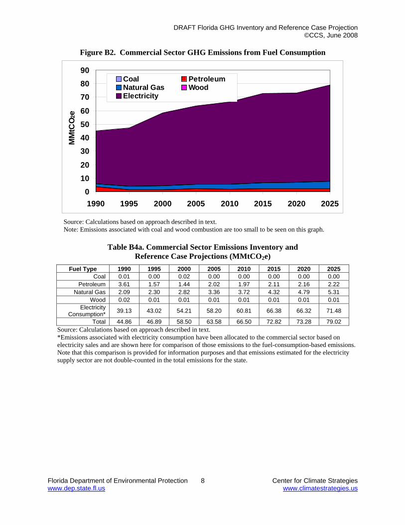
DRAFT Florida GHG Inventory and Reference Case Projection ©CCS, June 2008
Florida Department of Environmental Protection 8 Center for Climate Strategies www.dep.state.fl.us www.climatestrategies.us
Figure B2. Commercial Sector GHG Emissions from Fuel Consumption
01020
30405060
708090
1990 1995 2000 2005 2010 2015 2020 2025
MM
tCO 2
eCoal PetroleumNatural Gas WoodElectricity
Source: Calculations based on approach described in text. Note: Emissions associated with coal and wood combustion are too small to be seen on this graph.
Table B4a. Commercial Sector Emissions Inventory and
Reference Case Projections (MMtCO2e) Fuel Type 1990 1995 2000 2005 2010 2015 2020 2025
Coal 0.01 0.00 0.02 0.00 0.00 0.00 0.00 0.00 Petroleum 3.61 1.57 1.44 2.02 1.97 2.11 2.16 2.22
Natural Gas 2.09 2.30 2.82 3.36 3.72 4.32 4.79 5.31 Wood 0.02 0.01 0.01 0.01 0.01 0.01 0.01 0.01
Electricity Consumption* 39.13 43.02 54.21 58.20 60.81 66.38 66.32 71.48
Total 44.86 46.89 58.50 63.58 66.50 72.82 73.28 79.02 Source: Calculations based on approach described in text. *Emissions associated with electricity consumption have been allocated to the commercial sector based on electricity sales and are shown here for comparison of those emissions to the fuel-consumption-based emissions. Note that this comparison is provided for information purposes and that emissions estimated for the electricity supply sector are not double-counted in the total emissions for the state.

DRAFT Florida GHG Inventory and Reference Case Projection ©CCS, June 2008
Florida Department of Environmental Protection 9 Center for Climate Strategies www.dep.state.fl.us www.climatestrategies.us
Table B4b. Commercial Sector Proportions of Total Emissions by Fuel Type Fuel Type 1990 1995 2000 2005 2010 2015 2020 2025
Coal 0.0% 0.0% 0.0% 0.0% 0.0% 0.0% 0.0% 0.0% Petroleum 8.0% 3.3% 2.5% 3.2% 3.0% 2.9% 2.9% 2.8%
Natural Gas 4.7% 4.9% 4.8% 5.3% 5.6% 5.9% 6.5% 6.7% Wood 0.0% 0.02% 0.01% 0.01% 0.01% 0.01% 0.01% 0.0%
Electricity Consumption 87.2% 91.7% 92.7% 91.5% 91.4% 91.2% 90.5% 90.5%
Source: Calculations based on approach described in text. *Emissions associated with electricity consumption have been allocated to the commercial sector based on electricity sales and are shown here for comparison of those emissions to the fuel-consumption-based emissions. Note that this comparison is provided for information purposes and that emissions estimated for the electricity supply sector are not double-counted in the total emissions for the state. Note: The percentages shown in this table reflect the emissions for each fuel type as a percentage of total emissions shown in Table B4a.
Industrial Sector Figure B3 presents the emission inventory and reference case projections for the industrial sector. Figure B3 was developed from the emissions data in Table B5a. Table B5b show the relative contributions of emissions associated with each fuel type to total industrial sector emissions. For the industrial sector, emissions from electricity and direct fuel use in 1990 were 25 MMtCO2e and are estimated to increase to about 25 MMtCO2e by 2025. Emissions associated with the generation of electricity to meet industrial energy consumption demand accounted for about 47% of total industrial emissions in 1990, and are estimated to be about 41% of total industrial emissions by 2025. In 1990, natural gas consumption accounted for about 20% of total industrial emissions, and is estimated to account for about 16% of total industrial emissions by 2025. Coal consumption accounted for about 11% of total industrial emissions in 1990 and increased to 12% in 2025. In 1990, petroleum consumption accounted for about 21% of total industrial emissions, and is estimated to be about 29% of total industrial emissions in 2025. Emissions associated with wood consumption by the industrial sector are about 1% of industrial emissions in 1990 and 2% of industrial emissions in 2025. For the 20-year period from 2005 to 2025, industrial-sector GHG emissions associated with the use natural gas, wood, and coal are expected to increase at average annual rates of about 0.3%, 6.3%, and 0.6% respectively. Emissions associated with the use of electricity and petroleum are expected to decrease annually by about 0.9% and 0.1%, respectively. Total GHG emissions for the industrial sector decrease by an average of about 0.2% annually over the 20-year period.
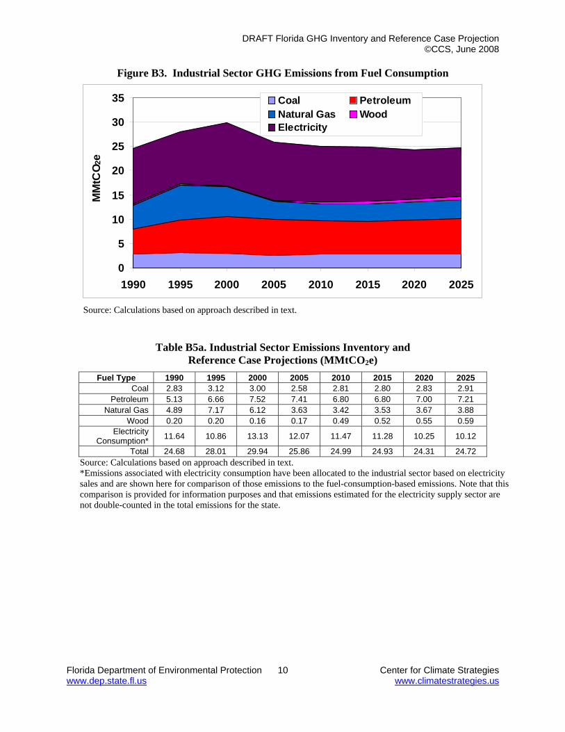
DRAFT Florida GHG Inventory and Reference Case Projection ©CCS, June 2008
Florida Department of Environmental Protection 10 Center for Climate Strategies www.dep.state.fl.us www.climatestrategies.us
Figure B3. Industrial Sector GHG Emissions from Fuel Consumption
0
5
10
15
20
25
30
35
1990 1995 2000 2005 2010 2015 2020 2025
MM
tCO 2
eCoal PetroleumNatural Gas WoodElectricity
Source: Calculations based on approach described in text.
Table B5a. Industrial Sector Emissions Inventory and Reference Case Projections (MMtCO2e)
Fuel Type 1990 1995 2000 2005 2010 2015 2020 2025 Coal 2.83 3.12 3.00 2.58 2.81 2.80 2.83 2.91
Petroleum 5.13 6.66 7.52 7.41 6.80 6.80 7.00 7.21 Natural Gas 4.89 7.17 6.12 3.63 3.42 3.53 3.67 3.88
Wood 0.20 0.20 0.16 0.17 0.49 0.52 0.55 0.59 Electricity
Consumption* 11.64 10.86 13.13 12.07 11.47 11.28 10.25 10.12
Total 24.68 28.01 29.94 25.86 24.99 24.93 24.31 24.72 Source: Calculations based on approach described in text. *Emissions associated with electricity consumption have been allocated to the industrial sector based on electricity sales and are shown here for comparison of those emissions to the fuel-consumption-based emissions. Note that this comparison is provided for information purposes and that emissions estimated for the electricity supply sector are not double-counted in the total emissions for the state.
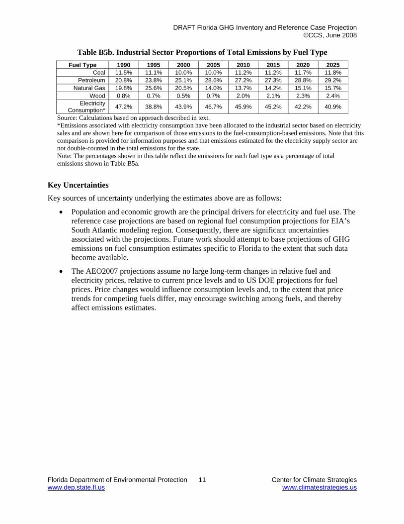
DRAFT Florida GHG Inventory and Reference Case Projection ©CCS, June 2008
Florida Department of Environmental Protection 11 Center for Climate Strategies www.dep.state.fl.us www.climatestrategies.us
Table B5b. Industrial Sector Proportions of Total Emissions by Fuel Type Fuel Type 1990 1995 2000 2005 2010 2015 2020 2025
Coal 11.5% 11.1% 10.0% 10.0% 11.2% 11.2% 11.7% 11.8% Petroleum 20.8% 23.8% 25.1% 28.6% 27.2% 27.3% 28.8% 29.2%
Natural Gas 19.8% 25.6% 20.5% 14.0% 13.7% 14.2% 15.1% 15.7% Wood 0.8% 0.7% 0.5% 0.7% 2.0% 2.1% 2.3% 2.4%
Electricity Consumption* 47.2% 38.8% 43.9% 46.7% 45.9% 45.2% 42.2% 40.9%
Source: Calculations based on approach described in text. *Emissions associated with electricity consumption have been allocated to the industrial sector based on electricity sales and are shown here for comparison of those emissions to the fuel-consumption-based emissions. Note that this comparison is provided for information purposes and that emissions estimated for the electricity supply sector are not double-counted in the total emissions for the state. Note: The percentages shown in this table reflect the emissions for each fuel type as a percentage of total emissions shown in Table B5a.
Key Uncertainties Key sources of uncertainty underlying the estimates above are as follows:
• Population and economic growth are the principal drivers for electricity and fuel use. The reference case projections are based on regional fuel consumption projections for EIA’s South Atlantic modeling region. Consequently, there are significant uncertainties associated with the projections. Future work should attempt to base projections of GHG emissions on fuel consumption estimates specific to Florida to the extent that such data become available.
• The AEO2007 projections assume no large long-term changes in relative fuel and electricity prices, relative to current price levels and to US DOE projections for fuel prices. Price changes would influence consumption levels and, to the extent that price trends for competing fuels differ, may encourage switching among fuels, and thereby affect emissions estimates.
DRAFT Florida GHG Inventory and Reference Case Projection ©CCS, June 2008
Florida Department of Environmental Protection 1 Center for Climate Strategies www.dep.state.fl.us www.climatestrategies.us
Annex C. Transportation Energy Use Overview Transportation is one the largest GHG source sectors in Florida. The transportation sector includes light- and heavy-duty (onroad) vehicles, aircraft, rail engines, and marine engines. Carbon dioxide (CO2) accounts for about 97% of the transportation sector’s GHG emissions in 1990, and about 98% in 2005 and 2025. Most of the remaining GHG emissions from the transportation sector are due to nitrous oxide (N2O) emissions from gasoline engines. Historical Emissions and Reference Case Projections Historical GHG emissions were estimated using the United States Environmental Protection Agency’s (US EPA) State Greenhouse Gas Inventory Tool (SIT) software and the methods provided in the Emission Inventory Improvement Program (EIIP) guidance document for the sector.41,42 For onroad vehicles, the CO2 emission factors are in units of pounds (lb) per million British thermal unit (MMBtu) and the methane (CH4) and N2O emission factors are both in units of grams per vehicle mile traveled (VMT). Key assumptions in this analysis are listed in Table C1. The default fuel consumption data within SIT were used to estimate emissions, with the most recently available fuel consumption data (2004 or 2005) from the United States Department of Energy (US DOE) Energy Information Administration’s (EIA) State Energy Data (SED) added.43 The default VMT data in SIT were replaced with annual VMT from the Florida Department of Transportation (DOT).44 Default data from the Federal Highway Administration (FHWA)45 were used to allocate the VMT to vehicle types. Onroad Vehicles Total annual VMT data for the years 1990 through 2005 were obtained from Florida DOT.46 These data were used to replace the default SIT VMT data for calculating CH4 and N2O emissions. The VMT data from Florida DOT were distributed to the SIT vehicle types in the same proportion as the default VMT data in the SIT. The default EIA SED data were used to calculate the CO2 emissions from onroad vehicles for the historical years. Gasoline consumption estimates for 1990-2005 were adjusted by subtracting ethanol consumption, per the methodology used in SIT. The historical EIA ethanol consumption data show that use of ethanol in Florida has declined from 0.13% of the gasoline consumption in 1990 to less than 0.001% in 2005. Florida ethanol distributors have plans to increase consumption of ethanol in the state to reach around
41 CO2 emissions were calculated using SIT, with reference to Emission Inventory Improvement Program, Volume VIII: Chapter. 1. “Methods for Estimating Carbon Dioxide Emissions from Combustion of Fossil Fuels”, August 2004. 42 CH4 and N2O emissions were calculated using SIT, with reference to Emission Inventory Improvement Program, Volume VIII: Chapter. 3. “Methods for Estimating Methane and Nitrous Oxide Emissions from Mobile Combustion”, August 2004. 43 Energy Information Administration, State Energy Consumption, Price, and Expenditure Estimates (SED), http://www.eia.doe.gov/emeu/states/_seds.html 44 VMT provided by Gordon Morgan, Transportation Statistics Office, Florida Department of Transportation. 45 Highway Statistics, Federal Highway Administration, http://www.fhwa.dot.gov/policy/ohpi/hss/index.htm. 46 VMT provided by Gordon Morgan, Transportation Statistics Office, Florida Department of Transportation.

DRAFT Florida GHG Inventory and Reference Case Projection ©CCS, June 2008
Florida Department of Environmental Protection 2 Center for Climate Strategies www.dep.state.fl.us www.climatestrategies.us
1% of gasoline consumption.47 However, for the reference case projections, ethanol consumption is assumed to remain at the 2005 consumption level (0.0005% of total gasoline consumption). Planned increases in ethanol consumption within the state may be included as a mitigation strategy. Onroad gasoline and diesel vehicle emissions were projected through 2025 based on statewide VMT growth rates developed by Florida DOT from linear extrapolation of the historical Florida 2001-2005 VMT data.48 The resulting total annual VMT data were then allocated by vehicle type based on national VMT forecasts by vehicle type reported in EIA’s Annual Energy Outlook 2007 (AEO2007).49 The AEO2007 data were incorporated because they indicate significantly different VMT growth rates for certain vehicle types (e.g., 24 percent growth between 2005 and 2025 in light-duty gasoline vehicle VMT versus 57 percent growth in heavy-duty diesel truck VMT over this period). The AEO2007 vehicle type-based national growth rates were applied to the 2005 Florida estimates of VMT by vehicle type. These VMT data were then proportionally adjusted to total to the projected statewide VMT totals for each year. The resulting vehicle-type VMT estimates and compound annual average growth rates are displayed in Tables C2 and C3, respectively. These VMT growth rates were used to forecast the CH4 and N2O emissions from onroad gasoline and diesel vehicles. For forecasting CO2 emissions, growth in fuel consumption is needed. The historical onroad gasoline and diesel fuel consumption data were forecasted through 2025 by developing a set of growth factors that adjusted the VMT projections shown in Table C3 to account for improvements in vehicle fuel efficiency. Projected calendar year fuel efficiency data were obtained from EPA. The resulting onroad fuel consumption growth rates are shown in Table C4. Growth rates for projecting CO2 emissions from natural gas and LPG vehicles were calculated by allocating the AEO2007 consumption of these fuels in the South Atlantic region and allocating this to Florida based on the ratio of the State’s projected population to the region’s projected population. The historic data for lubricants shows no significant positive or negative trend; therefore, no growth was assumed for lubricants.
47 Phase 1 Report: Florida’s Energy and Climate Change Action Plan, Governor’s Action Team on Energy and Climate Change, November 1, 2007 http://www.dep.state.fl.us/climatechange/files/20071101_final_report.pdf 48 Linear VMT projection provided to CCS by Kathy Neill, Director, Office of Policy Planning, Florida Department of Transportation, in Excel file “Annual VMT projection 032008.xls,” April 16, 2008. 49 US Department of Energy, Energy Information Administration, Annual Energy Outlook 2007 with Projections to 2030, DOE/EIA-0383(2007), February 2007, available at http://www.eia.doe.gov/oiaf/aeo/index.html.
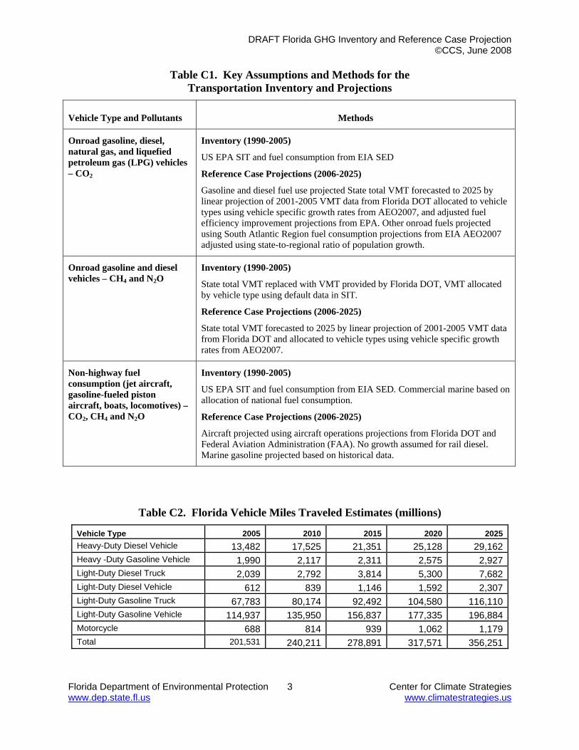
DRAFT Florida GHG Inventory and Reference Case Projection ©CCS, June 2008
Florida Department of Environmental Protection 3 Center for Climate Strategies www.dep.state.fl.us www.climatestrategies.us
Table C1. Key Assumptions and Methods for the Transportation Inventory and Projections
Vehicle Type and Pollutants Methods
Onroad gasoline, diesel, natural gas, and liquefied petroleum gas (LPG) vehicles – CO2
Inventory (1990-2005)
US EPA SIT and fuel consumption from EIA SED
Reference Case Projections (2006-2025)
Gasoline and diesel fuel use projected State total VMT forecasted to 2025 by linear projection of 2001-2005 VMT data from Florida DOT allocated to vehicle types using vehicle specific growth rates from AEO2007, and adjusted fuel efficiency improvement projections from EPA. Other onroad fuels projected using South Atlantic Region fuel consumption projections from EIA AEO2007 adjusted using state-to-regional ratio of population growth.
Onroad gasoline and diesel vehicles – CH4 and N2O
Inventory (1990-2005)
State total VMT replaced with VMT provided by Florida DOT, VMT allocated by vehicle type using default data in SIT.
Reference Case Projections (2006-2025)
State total VMT forecasted to 2025 by linear projection of 2001-2005 VMT data from Florida DOT and allocated to vehicle types using vehicle specific growth rates from AEO2007.
Non-highway fuel consumption (jet aircraft, gasoline-fueled piston aircraft, boats, locomotives) – CO2, CH4 and N2O
Inventory (1990-2005)
US EPA SIT and fuel consumption from EIA SED. Commercial marine based on allocation of national fuel consumption.
Reference Case Projections (2006-2025)
Aircraft projected using aircraft operations projections from Florida DOT and Federal Aviation Administration (FAA). No growth assumed for rail diesel. Marine gasoline projected based on historical data.
Table C2. Florida Vehicle Miles Traveled Estimates (millions)
Vehicle Type 2005 2010 2015 2020 2025 Heavy-Duty Diesel Vehicle 13,482 17,525 21,351 25,128 29,162Heavy -Duty Gasoline Vehicle 1,990 2,117 2,311 2,575 2,927Light-Duty Diesel Truck 2,039 2,792 3,814 5,300 7,682Light-Duty Diesel Vehicle 612 839 1,146 1,592 2,307Light-Duty Gasoline Truck 67,783 80,174 92,492 104,580 116,110Light-Duty Gasoline Vehicle 114,937 135,950 156,837 177,335 196,884Motorcycle 688 814 939 1,062 1,179Total 201,531 240,211 278,891 317,571 356,251

DRAFT Florida GHG Inventory and Reference Case Projection ©CCS, June 2008
Florida Department of Environmental Protection 4 Center for Climate Strategies www.dep.state.fl.us www.climatestrategies.us
Table C3. Florida Vehicle Miles Traveled Compound Annual Growth Rates
Vehicle Type 2005-2010 2010-2015 2015-2020 2020-2025 Heavy-Duty Diesel Vehicle 5.4% 4.0% 3.3% 3.0% Heavy-Duty Gasoline Vehicle 1.2% 1.8% 2.2% 2.6% Light-Duty Diesel Truck 6.5% 6.4% 6.8% 7.7% Light-Duty Diesel Vehicle 6.5% 6.4% 6.8% 7.7% Light-Duty Gasoline Truck 3.4% 2.9% 2.5% 2.1% Light-Duty Gasoline Vehicle 3.4% 2.9% 2.5% 2.1% Motorcycle 3.4% 2.9% 2.5% 2.1%
Table C4. Florida Onroad Fuel Consumption Compound Annual Growth Rates
Vehicle Type 2005-2010 2010-2015 2015-2020 2020-2025 Onroad gasoline 3.1% 2.7% 2.4% 2.1% Light-Duty Gasoline Vehicle 3.3% 2.9% 2.5% 2.1% Light-Duty Gasoline Truck 2.9% 2.6% 2.3% 2.0% Heavy-Duty Gasoline Vehicle 1.0% 1.6% 2.2% 2.6% Motorcycle 3.4% 2.9% 2.5% 2.1% Onroad diesel 5.1% 4.2% 3.6% 3.4% Light-Duty Diesel Vehicle 4.6% 6.4% 6.8% 7.7% Light-Duty Diesel Truck 5.9% 6.4% 6.6% 7.6% Heavy-Duty Diesel Vehicle 5.1% 4.0% 3.3% 3.0%
Aviation For the aircraft sector, emission estimates for 1990 to 2005 are based on SIT methods and fuel consumption from EIA. Emissions were projected from 2005 to 2025 using general aviation and commercial aircraft operations for 2005 through 2025 from Florida DOT50 and military operations for 2005 through 2025 from the Federal Aviation Administration’s (FAA) Terminal Area Forecast System51 and national aircraft fuel efficiency forecasts. To estimate changes in jet fuel consumption, aircraft operations from air carrier, air taxi/commuter, and military aircraft were first summed for each year of interest. The post-2005 estimates were adjusted to reflect the projected increase in national aircraft fuel efficiency (indicated by increased number of seat miles per gallon), as reported in AEO2007. Because AEO2007 does not estimate fuel efficiency changes for general aviation aircraft, forecast changes in aviation gasoline consumption were based solely on the projected number of itinerant general aviation aircraft operations in Florida, which was obtained from the FAA source noted above. The resulting compound annual average growth rates are displayed in Table C5.
50 Aviation Data and Forecasts, Florida Department of Transportation. http://www.dot.state.fl.us/aviation/dataforecasts.htm. 51 Terminal Area Forecast, Federal Aviation Administration, http://www.apo.data.faa.gov/main/taf.asp.

DRAFT Florida GHG Inventory and Reference Case Projection ©CCS, June 2008
Florida Department of Environmental Protection 5 Center for Climate Strategies www.dep.state.fl.us www.climatestrategies.us
Table C5. Florida Aviation Fuels Compound Annual Growth Rates
Fuel 2005-2010 2010-2015 2015-2020 2020-2025 Aviation Gasoline 0.8% 1.5% 1.5% 1.5% Jet Fuel 0.4% 1.7% 1.8% 1.9%
Rail and Marine Vehicles For the rail and recreational marine sectors, 1990-2005 estimates are based on SIT methods and fuel consumption from EIA. Marine gasoline consumption was projected to 2025 based on a linear regression of the 1990 through 2005 historical data. The historic data for rail shows no significant positive or negative trend; therefore, no growth was assumed for this sector. For the commercial marine sector (marine diesel and residual fuel), 1990-2005 emission estimates are based on SIT emission rates applied to estimates of Florida marine vessel diesel and residual fuel consumption. Because the SIT default marine fuel consumption data relies on marine vessel fuel consumption estimates that represent the State in which fuel is sold rather than consumed, an alternative method was used to estimate Florida marine vessel fuel consumption. Florida fuel consumption estimates were developed by allocating 1990-2005 national diesel and residual oil vessel bunkering fuel consumption estimates obtained from EIA.52 Marine vessel fuel consumption was allocated to Florida using the marine vessel activity allocation methods and data compiled to support the development of EPA’s National Emissions Inventory (NEI).53 In keeping with the NEI, 75% of each year’s distillate fuel and 25% of each year’s residual fuel were assumed to be consumed within the port area (remaining consumption was assumed to occur while ships are underway). National port area fuel consumption was allocated to Florida based on year-specific freight tonnage data by state as reported in “Waterborne Commerce of the United States, Part 5 – Waterways and Harbors National Summaries.”54 Offshore CO2 and hydrocarbon (HC) emissions for Florida’s exclusive economic zone (EEZ) were taken from a study by James Corbett for the Commission for Environmental Cooperation (CEC) in North America.55 Offshore CH4 emissions were estimated by speciating the HC emissions using the California Air Resources Board’s total organic gas (TOG) profile (#818).56 Offshore N2O emissions were estimated by applying the ratio of N2O to CH4 emission factors to the CH4 emission estimate. The 2002 offshore emissions from the CEC inventory were scaled to other historic years based on the estimated underway diesel and residual fuel consumption. Port and
52 US Department of Energy, Energy Information Administration, “Petroleum Navigator” (diesel data obtained from http://tonto.eia.doe.gov/dnav/pet/hist/kd0vabnus1a.htm; residual data obtained from http://tonto.eia.doe.gov/dnav/pet/hist/kprvatnus1a.htm). 53 See methods described in ftp://ftp.epa.gov/EmisInventory/2002finalnei/documentation/mobile/2002nei_mobile_nonroad_methods.pdf 54 Waterborne Commerce Statistics Center, http://www.iwr.usace.army.mil/ndc/wcsc/wcsc.htm. 55 Estimate, Validation, and Forecasts of Regional Commercial Marine Vessel Inventories, submitted by J. Corbett, prepared for the California Air Resources Board, California Environmental Protection Agency, and Commission for Environmental Cooperation in North America, http://coast.cms.udel.edu/NorthAmericanSTEEM/. 56 California Air Resources Board, Speciation Profiles, http://www.arb.ca.gov/ei/speciate/speciate.htm.

DRAFT Florida GHG Inventory and Reference Case Projection ©CCS, June 2008
Florida Department of Environmental Protection 6 Center for Climate Strategies www.dep.state.fl.us www.climatestrategies.us
offshore commercial marine emissions were projected using linear regression based on the 1990 through 2005 emission data.
Nonroad Engines It should be noted that fuel consumption data from EIA includes nonroad gasoline and diesel fuel consumption in the commercial and industrial sectors. Emissions from these nonroad engines, including nonroad vehicles such as dirt bikes, are included in the inventory and forecast for the residential, commercial, and industrial (RCI) sectors. Table C6 shows how EIA divides gasoline and diesel fuel consumption between the transportation, commercial, and industrial sectors.
Table C6. EIA Classification of Gasoline and Diesel Consumption
Sector Gasoline Consumption Diesel Consumption
Transportation Highway vehicles, marine Vessel bunkering, military use, railroad, highway vehicles
Commercial Public non-highway, miscellaneous use Commercial use for space heating, water heating, and cooking
Industrial Agricultural use, construction, industrial and commercial use
Industrial use, agricultural use, oil company use, off-highway vehicles
Results As shown in Figure C1 and in Table C7, onroad gasoline consumption accounts for the largest share of transportation GHG emissions. Emissions from onroad gasoline vehicles increased by about 44% from 1990 to 2005, accounting for 63% of total transportation emissions in 2005. GHG emissions from onroad diesel fuel consumption increased by 88% from 1990 to 2005, and by 2005 accounted for 15% of GHG emissions from the transportation sector. Emissions from boats and ships increased by 35% from 1990 to 2005 to account for 12% of transportation emissions in 2005. . Emissions from aviation decreased by 13% from 1990 to 2005 to account for 9% of transportation emissions in 2005. Emissions from all other categories combined (locomotives, natural gas, liquefied petroleum gas (LPG), and oxidation of lubricants) contributed about 1% of total transportation emissions in 2005. GHG emissions from onroad gasoline consumption are projected to increase by about 66%, and emissions from onroad diesel consumption are expected to increase by 123% between 2005 and 2025. Aviation emissions are projected to increase by 33% from 2005 to 2025, while marine emissions are projected to increase by 11% from 2005 to 2025.
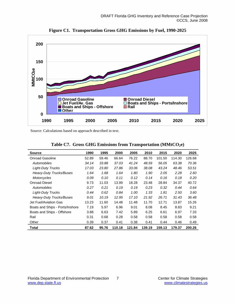
DRAFT Florida GHG Inventory and Reference Case Projection ©CCS, June 2008
Florida Department of Environmental Protection 7 Center for Climate Strategies www.dep.state.fl.us www.climatestrategies.us
Figure C1. Transportation Gross GHG Emissions by Fuel, 1990-2025
0
50
100
150
200
1990 1995 2000 2005 2010 2015 2020 2025
MM
tCO 2
e
Onroad Gasoline Onroad DieselJet Fuel/Av. Gas Boats and Ships - Ports/InshoreBoats and Ships - Offshore RailOther
Source: Calculations based on approach described in text.
Table C7. Gross GHG Emissions from Transportation (MMtCO2e)
Source 1990 1995 2000 2005 2010 2015 2020 2025 Onroad Gasoline 52.89 59.46 66.64 76.22 88.70 101.50 114.30 126.68 Automobiles 34.14 33.88 37.03 41.24 48.59 56.05 63.38 70.36 Light-Duty Trucks 17.03 23.80 27.86 33.06 38.08 43.24 48.46 53.51 Heavy-Duty Trucks/Buses 1.64 1.68 1.64 1.80 1.90 2.05 2.28 2.60 Motorcycles 0.09 0.10 0.11 0.12 0.14 0.16 0.18 0.20 Onroad Diesel 9.73 11.03 13.99 18.28 23.48 28.84 34.37 40.72 Automobiles 0.27 0.21 0.19 0.19 0.23 0.32 0.44 0.64 Light-Duty Trucks 0.44 0.62 0.84 1.00 1.33 1.81 2.50 3.60 Heavy-Duty Trucks/Buses 9.01 10.19 12.95 17.10 21.92 26.71 31.43 36.48 Jet Fuel/Aviation Gas 13.23 11.60 14.48 11.48 11.70 12.71 13.87 15.26 Boats and Ships - Ports/Inshore 7.19 5.97 6.96 9.01 8.08 8.45 8.83 9.21 Boats and Ships - Offshore 3.88 6.63 7.42 5.89 6.25 6.61 6.97 7.33 Rail 0.31 0.68 0.28 0.58 0.58 0.58 0.58 0.58 Other 0.39 0.37 0.41 0.38 0.41 0.44 0.46 0.49 Total 87.62 95.76 110.18 121.84 139.19 159.13 179.37 200.26
DRAFT Florida GHG Inventory and Reference Case Projection ©CCS, June 2008
Florida Department of Environmental Protection 8 Center for Climate Strategies www.dep.state.fl.us www.climatestrategies.us
Key Uncertainties
Uncertainties in Onroad Fuel Consumption A major uncertainty in this analysis is the conversion of the projected VMT to fuel consumption. The projected onroad fuel consumption calculation is based on first allocating Florida’s total VMT by vehicle type using national vehicle type growth projections from AEO2007 modeling, which may not reflect Florida conditions. The conversion of the VMT data to fuel consumption also includes national assumptions regarding fuel economy by vehicle type. Due to the large tourist industry in Florida, and the associated use of rental cars with the tourist industry, the Florida fleet may have a higher average fuel economy than the national fleet due to the use of relatively new vehicles in the rental car industry. If this is the case, then the onroad emissions growth may be overestimated for Florida. The Florida Department of Environmental Protection has recently obtained and processed vehicle registration data for Florida. The GHG emission projections may be revised in the future so that the GHG projections use a more realistic estimate of fleet turnover in Florida. . Energy Independence and Security Act of 2007 The reference case projections documented here do not include the corporate average fuel economy (CAFE) or biofuels provisions (or any other provisions) of the Energy Independence and Security Act of 2007. Increases in vehicle fuel economy resulting from this act would lead to reduced CO2 emissions from onroad vehicles. Reductions attributable to the CAFE and biofuels provisions of this Act will be separately quantified at a later date. Uncertainties in Aviation Fuel Consumption The jet fuel and aviation gasoline fuel consumption from EIA is actually fuel purchased in the State, and therefore, includes fuel consumed during state-to-state flights and international flights. The fuel consumption associated with international air flights should not be included in the State inventory; however, data were not available to subtract this consumption from total jet fuel estimates. Another uncertainty associated with aviation emissions is the use of general aviation forecasts to project aviation gasoline consumption. General aviation aircraft consume both jet fuel and aviation gasoline, but fuel specific data were not available. Uncertainties in Marine Fuel Consumption There are several assumptions that introduce uncertainty into the estimates of commercial marine fuel consumption. These assumptions include:
• 75% of marine diesel and 25% of residual fuel is consumed in port; and
• The proportion of freight tonnage at ports in Florida to the total national freight tonnage reflects the proportion of national marine fuel that is consumed in Florida.

DRAFT Florida GHG Inventory and Reference Case Projection ©CCS, June 2008
Florida Department of Environmental Protection 1 Center for Climate Strategies www.dep.state.fl.us www.climatestrategies.us
Annex D. Industrial Processes Overview Emissions in the industrial processes category span a wide range of activities, and reflect non-combustion sources of greenhouse gas (GHG) emissions from several industries. The industrial processes that exist in Florida, and for which emissions are estimated in this inventory, include the following:
• Carbon Dioxide (CO2) from:
- Production of cement, iron and steel, and ammonia;57
- Consumption of limestone, dolomite, and soda ash;
• Sulfur hexafluoride (SF6) from:
- Transformers used in electric power transmission and distribution (T&D) systems;
• Hydrofluorocarbons (HFCs) and perfluorocarbons (PFCs) from consumption of substitutes for ozone-depleting substances (ODS) used in cooling and refrigeration equipment; and
• HFCs, PFCs, and SF6 from semiconductor manufacture.
Other industrial processes that are sources of GHG emissions but are not found in Florida include the following:
• CO2 from lime production;
• Nitrous oxide (N2O) from nitric and adipic acid production;
• PFCs from aluminum production;
• SF6 from magnesium production and processing;
• HFCs from HCFC-22 production. Emissions and Reference Case Projections Greenhouse gas emissions for 1990 through 2005 were estimated using the United States Environmental Protection Agency’s (US EPA) State Greenhouse Gas Inventory Tool (SIT) software, and the methods provided in the Emission Inventory Improvement Program (EIIP) guidance document for this sector.58 Table D1 identifies for each emissions source category the information needed for input into SIT to calculate emissions, the data sources used for the analyses described here, and the historical years for which emissions were calculated based on the availability of data.
57 Note that CO2 emissions from urea application is estimated as part of the same category as ammonia production. 58 GHG emissions were calculated using SIT, with reference to EIIP, Volume VIII: Chapter. 6. “Methods for Estimating Non-Energy Greenhouse Gas Emissions from Industrial Processes”, August 2004. Referred to as “EIIP” below.

DRAFT Florida GHG Inventory and Reference Case Projection ©CCS, June 2008
Florida Department of Environmental Protection 2 Center for Climate Strategies www.dep.state.fl.us www.climatestrategies.us
Table D1. Approach to Estimating Historical Emissions
Source Category
Time Period for
which Data
Available Required Data
for SIT Data Source
Cement Manufacture
1990 - 2005
Metric tons (Mt) of clinker produced and masonry cement produced each year.
Historical production for Florida from United States Geological Survey (USGS) Minerals Yearbook, Cement Statistics and Information (http://minerals.usgs.gov/minerals/pubs/commodity/cement/index.html#myb).
Limestone and Dolomite Consumption
1994 - 2004
Mt of limestone and dolomite consumed.
Historical consumption (sales) for Florida from USGS Minerals Yearbook, Crushed Stone Statistics and Information, (http://minerals.usgs.gov/minerals/pubs/commodity/stone_crushed/). In SIT, the state's total limestone consumption (as reported by USGS) is multiplied by the ratio of national limestone consumption for industrial uses to total national limestone consumption. Additional information on these calculations, including a definition of industrial uses, is available in Chapter 6 of the EIIP guidance document. Default limestone production data are not available in SIT for 1990 – 1993 and for 2005; data for 1994 were used for 1990 – 1993 as a surrogate to fill in production data missing for these years; data for 2004 were used for 2005 production.
Soda Ash Consumption
1990 - 2005
Mt of soda ash consumed for use in consumer products such as glass, soap and detergents, paper, textiles, and food.
Historical emissions are calculated in SIT based on the state’s population and national per capita soda ash consumption from the US EPA national GHG inventory. -- National historical consumption (sales) for US from USGS Minerals Yearbook, Soda Ash Statistics and Information (http://minerals.usgs.gov/minerals/pubs/commodity/soda_ash/). -- US (1990-2000 and 2000-2005) and state (2000-2005) population from US Census Bureau (http://www.census.gov/popest/states/NST-ann-est.html). -- State (1990-2000) population from US Census Bureau (http://www.census.gov/popest/archives/2000s/vintage_2001/CO-EST2001-12/CO-EST2001-12-12.html).
Ammonia Production and Urea Consumption
1990-2004 Mt of Ammonia produced and Urea consumed in the state.
SIT default activity data for ammonia production and urea application for 1990-2004; activity data is based on national USGS data. No data was available for 2005, so 2004 production data was used as a surrogate for 2005 production.
Iron and Steel Production
1997-2005 Mt of crude steel produced by production method.
The basic activity data needed are the quantities of crude steel produced (defined as first cast product suitable for sale or further processing) by production method. Default SIT values are based on the state-level production data assigned to production method based on the national distribution of production by method. National production data are from the Annual Statistics Report published by the American Iron and Steel Institute, Washington, DC (http://www.steel.org/AM/Template.cfm?Section=Bookstore&CONTENTID=12259&TEMPLATE=/CM/HTMLDisplay.cfm). Default production data are not available in SIT for 1990-1996; 1997 production data were used as surrogate for 1990-1996 production.
ODS Substitutes
1990 - 2005
Based on state’s population and estimates of emissions per capita from the US EPA national GHG inventory.
National emissions from US Inventory of Greenhouse Gas Emissions and Sinks: 1990-2005, US EPA, Report #430-R-07-002, April 2007 (http://epa.gov/climatechange/emissions/ usinventoryreport.html). References for US Census Bureau national and state population figures are cited under the data sources for soda ash above.
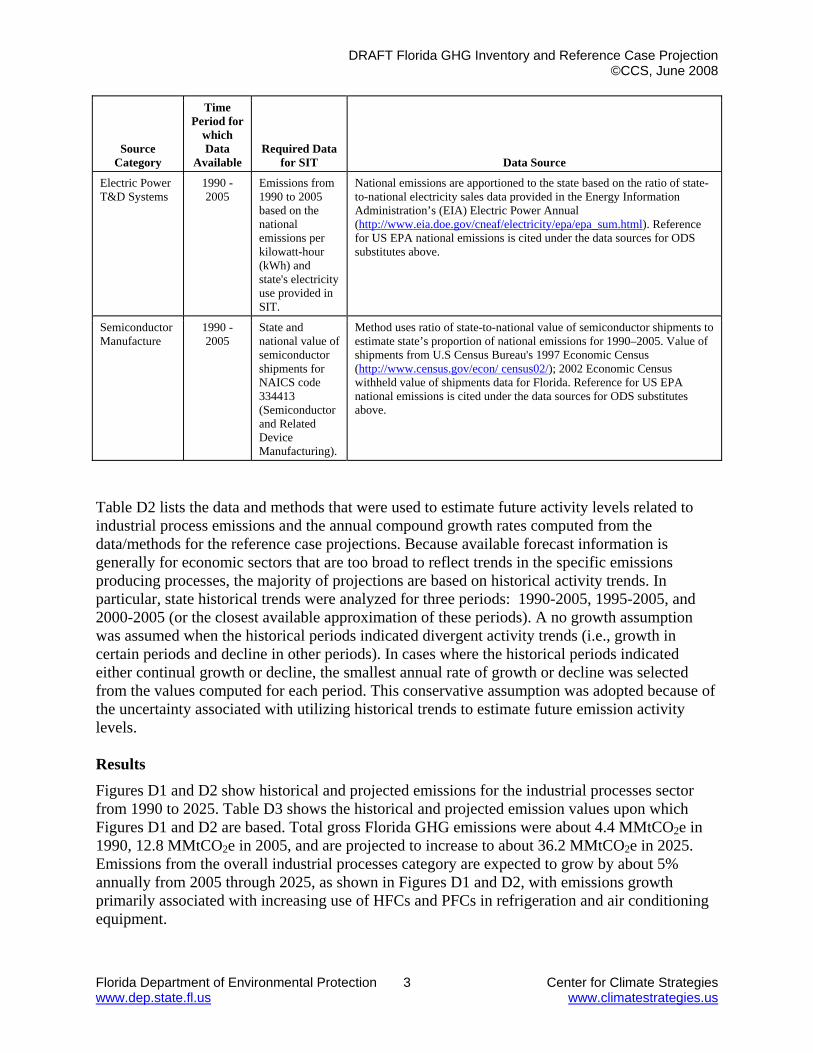
DRAFT Florida GHG Inventory and Reference Case Projection ©CCS, June 2008
Florida Department of Environmental Protection 3 Center for Climate Strategies www.dep.state.fl.us www.climatestrategies.us
Source Category
Time Period for
which Data
Available Required Data
for SIT Data Source
Electric Power T&D Systems
1990 - 2005
Emissions from 1990 to 2005 based on the national emissions per kilowatt-hour (kWh) and state's electricity use provided in SIT.
National emissions are apportioned to the state based on the ratio of state-to-national electricity sales data provided in the Energy Information Administration’s (EIA) Electric Power Annual (http://www.eia.doe.gov/cneaf/electricity/epa/epa_sum.html). Reference for US EPA national emissions is cited under the data sources for ODS substitutes above.
Semiconductor Manufacture
1990 - 2005
State and national value of semiconductor shipments for NAICS code 334413 (Semiconductor and Related Device Manufacturing).
Method uses ratio of state-to-national value of semiconductor shipments to estimate state’s proportion of national emissions for 1990–2005. Value of shipments from U.S Census Bureau's 1997 Economic Census (http://www.census.gov/econ/ census02/); 2002 Economic Census withheld value of shipments data for Florida. Reference for US EPA national emissions is cited under the data sources for ODS substitutes above.
Table D2 lists the data and methods that were used to estimate future activity levels related to industrial process emissions and the annual compound growth rates computed from the data/methods for the reference case projections. Because available forecast information is generally for economic sectors that are too broad to reflect trends in the specific emissions producing processes, the majority of projections are based on historical activity trends. In particular, state historical trends were analyzed for three periods: 1990-2005, 1995-2005, and 2000-2005 (or the closest available approximation of these periods). A no growth assumption was assumed when the historical periods indicated divergent activity trends (i.e., growth in certain periods and decline in other periods). In cases where the historical periods indicated either continual growth or decline, the smallest annual rate of growth or decline was selected from the values computed for each period. This conservative assumption was adopted because of the uncertainty associated with utilizing historical trends to estimate future emission activity levels. Results
Figures D1 and D2 show historical and projected emissions for the industrial processes sector from 1990 to 2025. Table D3 shows the historical and projected emission values upon which Figures D1 and D2 are based. Total gross Florida GHG emissions were about 4.4 MMtCO2e in 1990, 12.8 MMtCO2e in 2005, and are projected to increase to about 36.2 MMtCO2e in 2025. Emissions from the overall industrial processes category are expected to grow by about 5% annually from 2005 through 2025, as shown in Figures D1 and D2, with emissions growth primarily associated with increasing use of HFCs and PFCs in refrigeration and air conditioning equipment.

DRAFT Florida GHG Inventory and Reference Case Projection ©CCS, June 2008
Florida Department of Environmental Protection 4 Center for Climate Strategies www.dep.state.fl.us www.climatestrategies.us
Table D2. Approach to Estimating Projections for 2005 through 2025
Source Category Projection Assumptions Data Source
Annual Growth Rates (%) 2005 to
2010 2010 to
2015 2015 to
2020 2020 to
2025 Cement Manufacture
Smallest historical annual increase in state production from each of three periods analyzed (1990-2005).
Annual change in Florida clinker & masonry cement production: 1990-2005 = +5.7%; 1995-2005 = +6.9%; and 2000-2005 = +9.2%
5.7 5.7 5.7 5.7
Limestone and Dolomite Consumption
Annual growth rate computed from Nonmetallic Mineral Product Manufacturing sector employment forecast for state.
2007-2015 employment projections from Florida Agency for Workforce Innovation http://labormarketinfo.com/library/ep.htm.
1.4 1.4 1.4 1.4
Soda Ash Consumption
Smallest historical annual increase in state consumption from each of three periods analyzed (2000-2005).
Annual change in Florida soda ash consumption: 1990-2005 = +0.6%; 1995-2005 = +0.6%; and 2000-2005 = +0.4%
0.4 0.4 0.4 0.4
Ammonia Production and Urea Application
No growth assumption based on analysis of state historical production/consumption trends.
Annual change in Florida ammonia production and urea consumption: 1990-2004 = -2.3%; 1995-2004 = +4.4%; and 2000-2004 = +2.2%
0 0 0 0
Iron and Steel Production
Annual growth rate computed from Primary Metal Mfg sector employment forecast for state.
2007-2015 employment projections from Florida Agency for Workforce Innovation http://labormarketinfo.com/library/ep.htm.
0.5 0.5 0.5 0.5
ODS Substitutes National growth in emissions associated with the use of ODS substitutes.
Annual growth rates calculated based on sum of US national emissions projections from 2005-2020 for six categories of ODS substitutes presented in Appendix D, Tables D1 through D-6 in the US EPA report, Global Anthropogenic Emissions of Non-CO2 Greenhouse Gases 1990-2020, EPA Report 430-R-06-003, http://www.epa.gov/nonco2/econ-inv/international.html.
8.7 6.4 5.0 5.0
Electric Power T&/D Systems
National growth rate (based on technology adoption forecast scenario reflecting industry participation in EPA voluntary stewardship program to control emissions).
Annual growth rates calculated based on US national emissions projections from 2005-2020 presented in Appendix D, Table D8 in the US EPA report, Global Anthropogenic Emissions of Non-CO2 Greenhouse Gases 1990-2020 , EPA Report 430-R-06-003; http://www.epa.gov/nonco2/econ-inv/international.html.
-1.6 -0.8 -0.7 -0.7
Semiconductor Manufacturing
National growth rate (based on technology adoption forecast scenario reflecting industry participation in EPA voluntary stewardship program to control emissions).
Annual growth rates calculated based on US national emissions projections from 2005-2020 presented in Appendix D, Table D10 in the US EPA report, Global Anthropogenic Emissions of Non-CO2 Greenhouse Gases 1990-2020 , EPA Report 430-R-06-003; http://www.epa.gov/nonco2/econ-inv/international.html.
0.7 -4.2 -1.4 -1.4

DRAFT Florida GHG Inventory and Reference Case Projection ©CCS, June 2008
Florida Department of Environmental Protection 5 Center for Climate Strategies www.dep.state.fl.us www.climatestrategies.us
Cement Manufacture The cement production process is one that releases relatively high amounts of CO2 in the industrial non-fuel combustion sector. Clinker is an intermediate product from which finished Portland and masonry cement are made. Clinker production releases CO2 when calcium carbonate (CaCO3) is heated in a cement kiln to form lime (calcium oxide) and CO2 (see Chapter 6 of EIIP guidance document). Emissions are calculated by multiplying annual clinker production by emission factors to estimate emissions associated with the clinker production process (0.507 metric ton (Mt) of CO2 emitted per Mt of clinker produced) and cement kiln dust (0.020 MtCO2e emitted per Mt of clinker produced). Masonry cement requires additional lime, over and above the lime used in the clinker. During the production of masonry cement, non-plasticizer additives such as lime, slag, and shale are added to the cement, increasing its weight by 5%. Lime accounts for approximately 60% of the added substances. About 0.0224 MtCO2 is emitted for every Mt of masonry cement produced, relative to the CO2 emitted during the production of a Mt of clinker (see Chapter 6 of EIIP guidance document). As shown in Figure D2 (see black line) and Table D3, emissions from this source are estimated to be about 1.2 MMtCO2e in 1990, 2.8 MMtCO2e in 2005, and are projected to increase to about 8.3 MMtCO2e by 2025. Historical clinker and masonry cement production data for Florida obtained from the United States Geological Survey (USGS) (see Table D1) and the default emission factors in SIT were used to calculate CO2 emissions for 1990-2005. The annual rate of increase in Florida clinker/masonry cement production over the 1990-2005 period (5.7% per year) was used to project emissions from 2006 to 2025.
Figure D1. GHG Emissions from Industrial Processes, 1990-2025
0
5
10
15
20
25
30
35
40
1990 1995 2000 2005 2010 2015 2020 2025Year
MM
tCO
2e
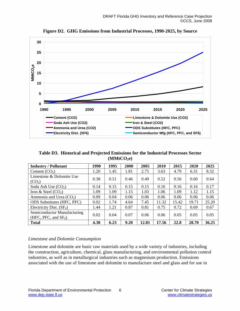
DRAFT Florida GHG Inventory and Reference Case Projection ©CCS, June 2008
Florida Department of Environmental Protection 6 Center for Climate Strategies www.dep.state.fl.us www.climatestrategies.us
Figure D2. GHG Emissions from Industrial Processes, 1990-2025, by Source
0
5
10
15
20
25
30
1990 1995 2000 2005 2010 2015 2020 2025
MM
tCO
2e
Cement (CO2) Limestone & Dolomite Use (CO2)Soda Ash Use (CO2) Iron & Steel (CO2)Ammonia and Urea (CO2) ODS Substitutes (HFC, PFC)Electricity Dist. (SF6) Semiconductor Mfg (HFC, PFC, and SF6)
Table D3. Historical and Projected Emissions for the Industrial Processes Sector (MMtCO2e)
Industry / Pollutant 1990 1995 2000 2005 2010 2015 2020 2025 Cement (CO2) 1.20 1.45 1.81 2.75 3.63 4.79 6.31 8.32 Limestone & Dolomite Use (CO2)
0.38 0.51 0.46 0.49 0.52 0.56 0.60 0.64
Soda Ash Use (CO2) 0.14 0.15 0.15 0.15 0.16 0.16 0.16 0.17 Iron & Steel (CO2) 1.09 1.09 1.15 1.03 1.06 1.09 1.12 1.15 Ammonia and Urea (CO2) 0.09 0.04 0.06 0.06 0.06 0.06 0.06 0.06 ODS Substitutes (HFC, PFC) 0.02 1.74 4.64 7.45 11.32 15.42 19.71 25.20 Electricity Dist. (SF6) 1.44 1.21 0.87 0.81 0.75 0.72 0.69 0.67 Semiconductor Manufacturing (HFC, PFC, and SF6)
0.02 0.04 0.07 0.06 0.06 0.05 0.05 0.05
Total 4.38 6.23 9.20 12.81 17.56 22.8 28.70 36.25 Limestone and Dolomite Consumption
Limestone and dolomite are basic raw materials used by a wide variety of industries, including the construction, agriculture, chemical, glass manufacturing, and environmental pollution control industries, as well as in metallurgical industries such as magnesium production. Emissions associated with the use of limestone and dolomite to manufacture steel and glass and for use in
DRAFT Florida GHG Inventory and Reference Case Projection ©CCS, June 2008
Florida Department of Environmental Protection 7 Center for Climate Strategies www.dep.state.fl.us www.climatestrategies.us
flue-gas desulfurization scrubbers to control sulfur dioxide emissions from the combustion of coal in boilers are included in the industrial processes sector.59 Historical limestone and dolomite consumption (sales) data for Florida obtained from the USGS (see Table D1) and the default emission factors in SIT were used to calculate CO2 emissions for 1990-2005. Data on limestone and dolomite consumption for 1990-1993 were not available for Florida; therefore, 1994 production data were used as a surrogate to estimate emissions for 1990-1993. Limestone and dolomite consumption for 2005 were also not available, 2004 production data were used as a surrogate. Relative to total industrial non-combustion process emissions, CO2 emissions from limestone and dolomite consumption are low (0.38 MMtCO2e in 1990, 0.49 MMtCO2e in 2005). Emission projections from 2005 to 2025 are assumed to increase at a rate of 1.4 percent per year to 0.64 MMtCO2e in 2025; this is based on Nonmetallic Mineral Product Manufacturing sector employment projections available from the State of Florida (note that these projections are available for 2015—in lieu of other information, the same rate of increase was used throughout the forecast period to 2025). Soda Ash Consumption
Commercial soda ash (sodium carbonate) is used in many consumer products such as glass, soap and detergents, paper, textiles, and food. Carbon dioxide is also released when soda ash is consumed (see Chapter 6 of EIIP guidance document). SIT estimates historical emissions (see dark pink line in Figure D2) based on the state’s population and national per capita soda ash consumption from the US EPA national GHG inventory. An annual 0.4 percent increase was assumed for the forecast period based on the positive consumption trends observed over the historical periods analyzed. Relative to total industrial non-combustion process emissions, CO2 emissions from soda ash consumption are low (about 0.14 MMtCO2e in 1990, 0.15 MMtCO2e in 2005, and increasing to 0.17 MMtCO2e in 2025) and therefore, appear at the bottom of the graph in Figure D2 (see pink line at the bottom of Figure D2). Ammonia Production/Urea Application
Ammonia (NH3) and urea ((NH2)2CO) are both synthetically created chemicals with a wide variety of uses. Ammonia is primarily used as a fertilizer, though it also has applications as a refrigerant, a disinfectant, and in the production of chemicals such as urea and nitric acid. Ammonia production involves the conversion of a fossil fuel hydrocarbon into pure hydrogen, which is then combined with nitrogen to create NH3. This process involves the release of carbon dioxide as a byproduct. Urea, a different type of synthetic chemical, is also primarily used as a fertilizer, though it is also used commercially in several industrial and chemical processes. Urea is created by a chemical process with ammonia as a key component. Ammonia and urea are typically produced from conventional catalytic reforming of natural gas feedstock. Default SIT activity data were used to calculate the ammonia and urea emissions in
59 In accordance with EIIP Chapter 6 methods, emissions associated with the following uses of limestone and dolomite are not included in this category: (1) crushed limestone consumed for road construction or similar uses (because these uses do not result in CO2 emissions), (2) limestone used for agricultural purposes (which is counted under the methods for the agricultural sector), and (3) limestone used in cement production (which is counted in the methods for cement production).

DRAFT Florida GHG Inventory and Reference Case Projection ©CCS, June 2008
Florida Department of Environmental Protection 8 Center for Climate Strategies www.dep.state.fl.us www.climatestrategies.us
Florida. Relative to total industrial non-combustion process emissions, CO2 emissions from ammonia production/urea application are low (about 0.09 MMtCO2e in 1990, decreasing to 0.06 MMtCO2e in 2005) and cannot be seen in Figure D2. A no growth assumption was adopted for this category based on the conflicting trends observed over the historical periods analyzed. Iron and Steel Production
The production of iron and steel generate process-related CO2 emissions. Iron is produced by reducing iron ore with metallurgical coke in a blast furnace to produce pig iron; this process emits CO2 emissions. Pig iron is used as a raw material in the production of steel. The production of metallurgical coke from coking coal produces CO2 emissions as well. Historical CO2 emissions were estimated using the SIT default activity data (see Table D1) for 1997-2005 and emission factors for the following production methods: basic oxygen furnace at integrated mill with coke ovens, basic oxygen furnace at integrated mill without coke ovens, electric arc furnace, and open hearth furnace. The basic activity data needed are the quantities of crude steel produced (defined as first cast product suitable for sale or further processing) by production method. Default values are based on the state-level production data assigned to each production method based on the national distribution of production by method. The national production data were obtained from the Annual Statistics Report published by the American Iron and Steel Institute, Washington, DC (see Table D1). Production data are not available in SIT for 1990-1996; data for these years are based on 1997 production. As shown in Figure D2 (see green line) and Table D3, emissions in 1990 were 1.09 MMtCO2e and decline to about 1.03 MMtCO2e in 2005. Post-2005 emissions are projected to increase at a rate of 0.5% per year based on Primary Metal Manufacturing sector employment projections available from the State of Florida (note that these projections are available for 2017—in lieu of other information, the same rate of decrease was used throughout the forecast period to 2025). Substitutes for Ozone-Depleting Substances (ODS)
HFCs and PFCs are used as substitutes for ODS, most notably chlorofluorocarbons (CFCs are also potent warming gases, with global warming potentials on the order of thousands of times that of CO2 per unit of emissions) in compliance with the Montreal Protocol and the Clean Air Act Amendments of 1990.60 Even low amounts of HFC and PFC emissions, for example, from leaks and other releases associated with normal use of the products, can lead to high GHG emissions on a CO2e basis. Emissions have increased from 0.02 MMtCO2e in 1990 to about 7.45 MMtCO2e in 2005, and are expected to increase at an average rate of 6.3% per year from 2005 to 2025 due to increased substitutions of these gases for ODS (see blue line in Figure D2). The projected rate of increase for these emissions is based on projections for national emissions from the US EPA report referenced in Table D2. Electric Power Transmission and Distribution 60 As noted in EIIP Chapter 6, ODS substitutes are primarily associated with refrigeration and air conditioning, but also many other uses including as fire control agents, cleaning solvents, aerosols, foam blowing agents, and in sterilization applications. The applications, stocks, and emissions of ODS substitutes depend on technology characteristics in a range of equipment types. For the US national inventory, a detailed stock vintaging model was used to track ODS substitutes uses and emissions, but this modeling approach has not been completed at the state level.

DRAFT Florida GHG Inventory and Reference Case Projection ©CCS, June 2008
Florida Department of Environmental Protection 9 Center for Climate Strategies www.dep.state.fl.us www.climatestrategies.us
Emissions of SF6 from electrical equipment have experienced declines since the mid-1990s (see dark blue line in Figure D2), mostly due to voluntary action by industry. Sulfur hexafluoride is used as an electrical insulator and interrupter in the electric power T&D system. The largest use for SF6 is as an electrical insulator in electricity T&D equipment, such as gas-insulated high-voltage circuit breakers, substations, transformers, and transmission lines, because of its high dielectric strength and arc-quenching abilities. Not all of the electric utilities in the US use SF6; use of the gas is more common in urban areas where the space occupied by electric power T&D facilities is more valuable.61 As shown in Figure D2 and Table D3, SF6 emissions from electric power T&D are about 1.44 MMtCO2e in 1990 and 0.81 MMtCO2e in 2005. Emissions in Florida from 1990 to 2005 were estimated based on the estimates of emissions per kilowatt-hour (kWh) of electricity consumed from the US EPA GHG inventory, and the ratio of Florida’s to the US electricity consumption (sales) estimates available from the Energy Information Administration’s (EIA) Electric Power Annual and provided in the SIT (see Table D1). The national trend in US emissions estimated for 2005-2025 for the technology-adoption scenario shows expected decreases in these emissions at the national level (see Table D2), and the same rate of decline is assumed for emissions in Florida. The decline in SF6 emissions in the future reflects expectations of future actions by the electric power industry to reduce these emissions. Semiconductor Manufacture
The semiconductor industry uses fluorinated gases (PFCs [CF4, C2F6, and C3F8]; HFC-23; and SF6) in plasma etching and chemical vapor deposition processes. Emissions of SF6 and HFCs from the manufacture of semiconductors have experienced declines since 2000. Emissions for Florida from 1990 to 2005 were estimated based on the default estimates provided in SIT, which uses the ratio of the state-to-national value of semiconductor shipments to estimate the state’s proportion of national emissions from the US EPA GHG inventory (see Table D1). The national trend in US emissions estimated for 2005-2025 for the technology-adoption scenario shows expected decreases in these emissions at the national level (see Table D2), and the same rate of decline is assumed for emissions in Florida. The projected emissions decrease reflects expectations of future actions by the semiconductor industry to reduce these emissions. Relative to total industrial non-combustion process emissions, estimated emissions associated with semiconductor manufacturing are low (about 0.02 MMtCO2e in 1990 and 0.06 MMtCO2e in 2005, and therefore, cannot be seen in Figure D2). Key Uncertainties
Key sources of uncertainty underlying the estimates above are as follows:
• Since emissions from industrial processes are determined by the level of production and the production processes of a few key industries—and in some cases, a few key plants—there is relatively high uncertainty regarding future emissions from the industrial processes category as a whole. Future emissions depend on the competitiveness of
61 US EPA, Draft User’s Guide for Estimating Carbon Dioxide, Nitrous Oxide, HFC, PFC, and SF6 Emissions from Industrial Processes Using the State Inventory Tool, prepared by ICF International, March 2007.
DRAFT Florida GHG Inventory and Reference Case Projection ©CCS, June 2008
Florida Department of Environmental Protection 10 Center for Climate Strategies www.dep.state.fl.us www.climatestrategies.us
Florida manufacturers in these industries, and the specific nature of the production processes used in Florida.
• The projected largest source of future industrial emissions, HFCs and PFCs used in cooling applications, is subject to several uncertainties as well. Emissions through 2025 and beyond will be driven by future choices regarding mobile and stationary air conditioning technologies and the use of refrigerants in commercial applications, for which several options currently exist.
• Due to the lack of reasonably specific projection surrogates, historical trend data were used to project emission activity level changes for multiple industrial processes. There is significant uncertainty associated with any projection, including a projection that assumes that past historical trends will continue in future periods. All assumptions on growth should be reviewed by industry experts and revised to reflect their expertise on future trends especially for the cement manufacturing industry, and for limestone and dolomite consumption and ODS substitutes.
• For the industries for which EPA default activity data and methods were used to estimate historical emissions, future work should include efforts to obtain state-specific data to replace the default assumptions. In cases where no data exists at all, the nearest year available can be used as a surrogate, but this decreases the overall accuracy of the inventory. Replacing as much default data with state-specific information from all years will significantly increase the reliability of the inventory.
• For the electricity T&D and semiconductor industries, future efforts should include a survey of companies within these industries to determine the extent to which they are implementing techniques to minimize emissions to improve the emission projections for these industries.

DRAFT Florida GHG Inventory and Reference Case Projection ©CCS, June 2008
Florida Department of Environmental Protection 1 Center for Climate Strategies www.dep.state.fl.us www.climatestrategies.us
Annex E. Fossil Fuel Industries
Overview The inventory for this subsector of the Energy Supply sector includes methane (CH4), nitrous oxide (N2O), and carbon dioxide (CO2) emissions associated with the production, processing, transmission, and distribution of fossil fuels in Florida.62 There is no coal mining in Florida. In 2005, emissions from this subsector accounted for an estimated 1.55 million metric tons (MMt) of CO2 equivalent (CO2e) of total gross greenhouse gas (GHG) emissions in Florida, and are estimated to increase to about 2.09 MMtCO2e by 2025. Emissions and Reference Case Projections
Oil and Gas Production
In 2005, Florida crude oil production totaled 7,000 barrels (bbls) per day, accounting for only 0.1% of US production.63 Proved crude oil reserves are 58 million bbls, which is similarly about 0.2% of US totals.64 The first year that the Energy Information Administration of the United States (US) Department of Energy reported production data for Florida (1981) was the peak year of oil production in the state (95,000 bbls per day). Production dropped dramatically in the 1980s and has steadily declined during the last two decades.65 Florida has no operating petroleum refineries. The majority of Florida’s natural gas is imported from neighboring states, but the state has limited internal production. All of the natural gas produced in Florida is associated gas. Associated gas is produced as a by-product in oil wells, as opposed to non-associated gas, which is produced in natural gas and condensate wells. In 2005, Florida consumed about 778 billion cubic feet (Bcf) of natural gas while it produced only about 2.6 Bcf.66
Oil and Gas Industry Emissions
Emissions can occur at several stages of production, processing, transmission, and distribution of oil and gas. Based on the information provided in the Emission Inventory Improvement Program (EIIP) guidance67 for estimating emissions for this sector, transmission pipelines are large diameter, high-pressure lines that transport gas from production fields, processing plants, storage facilities, and other sources of supply over long distances to local distribution companies or to large volume customers. Sources of CH4 emissions from transmission pipelines include leaks, 62 Note that emissions from natural gas consumed as lease fuel (used in well, field, and lease operations) and plant fuel (used in natural gas processing plants) are included in Annex B in the industrial fuel combustion category. 63 US Department of Energy (DOE), Energy Information Administration, “Crude Oil Production,” accessed from http://tonto.eia.doe.gov/dnav/pet/pet_crd_crpdn_adc_mbblpd_a.htm, January 2008. 64 US DOE, Energy Information Administration, “Crude Oil Proved Reserves, Reserves Changes, and Production,” accessed from http://tonto.eia.doe.gov/dnav/pet/pet_crd_pres_dcu_SFL_a.htm, January 2008. 65 “Petroleum Navigator”, US DOE Energy Information Administration website, January 2008, accessed from http://tonto.eia.doe.gov/dnav/pet/hist/mcrfpfl2a.htm. 66 “State Energy Profiles: Florida”, US DOE Energy Information Administration website, January 2008, accessed from http://tonto.eia.doe.gov/state/state_energy_profiles.cfm?sid=FL. 67 Emission Inventory Improvement Program, Volume VIII: Chapter 5. “Methods for Estimating Methane Emissions from Natural Gas and Oil Systems,” August 2004.
DRAFT Florida GHG Inventory and Reference Case Projection ©CCS, June 2008
Florida Department of Environmental Protection 2 Center for Climate Strategies www.dep.state.fl.us www.climatestrategies.us
compressor fugitives, vents, and pneumatic devices. Distribution pipelines are extensive networks of generally small diameter, low-pressure pipelines that distribute gas within cities or towns. Sources of CH4 emissions from distribution pipelines are leaks, meters, regulators, and mishaps. Carbon dioxide, CH4, and N2O emissions occur as the result of the combustion of natural gas by internal combustion engines used to operate compressor stations. With nearly 28,000 miles of gas pipelines, there are inevitable uncertainties associated with estimates of Florida’s GHG emissions from this sector. This is compounded by the fact that there are no regulatory requirements to track GHG emissions. However, the EPA’s State Greenhouse Gas Inventory Tool (SIT) facilitates the development of a rough estimate of state-level GHG emissions. Emission estimates are calculated by multiplying emissions-related activity levels (e.g., miles of pipeline, number of compressor stations) by aggregate industry-average emission factors. Key information sources for the activity data are the US Department of Energy’s Energy Information Administration (EIA),68 the US Department of Transportation’s Office of Pipeline Safety (OPS), 69 and the Florida Department of Environmental Protection (Florida DEP).70 Florida Public Service Commission (PSC) staff provided additional information, including direction as to the preferred data source in cases where more than one set of activity estimates was available. Methane emissions were estimated using the SIT, with reference to methods and data sources outlined in the EIIP guidance document for natural gas and oil systems.71 Emissions of CO2, CH4, and N2O associated with pipeline natural gas combustion were estimated using SIT emission factors72 and Florida 1990-2005 natural gas data from EIA for the “consumed as pipeline fuel” category.73 Unfortunately, OPS has not collected data from pipeline operators using a consistent set of reporting requirements over the 1990-2005 analysis period. In particular, OPS has only required operators to report state-level data for their transmission pipelines since 2001 and state-level data for their distribution pipelines since 2004. Before these dates, a large number of Florida pipeline records report data as multi-state totals. The Florida PSC was able to provide replacement data for natural gas distribution pipeline mileage and service counts that did not face the same issues. To estimate a complete time-series of natural gas gathering/transmission pipeline mileage, surrogate data were compiled to back-cast the 2001 gathering/transmission pipeline mileage for each year back to 1990.74
68 “Natural Gas Navigator,” US DOE Energy Information Administration website, January 2008, accessed from http://www.eia.doe.gov. 69 US Department of Transportation, Office of Pipeline Safety, “Distribution and Transmission Annuals Data: 1990 to 2005,” accessed from http://ops.dot.gov/stats/DT98.htm, January 2008. 70 “Access Database: Oil and Gas,” David Taylor, Florida Department of Environmental Protection, Bureau of Mining & Minerals Regulation, Oil and Gas Section, January 29, 2008. 71 Emission Inventory Improvement Program, Volume VIII: Chapter. 5. “Methods for Estimating Methane Emissions from Natural Gas and Oil Systems”, August 2004. 72 GHG emissions were calculated using SIT, with reference to EIIP, Volume VIII: Chapter 1 “Methods for Estimating Carbon Dioxide Emissions from Combustion of Fossil Fuels,” August 2004, and Chapter 2 “Methods for Estimating Methane and Nitrous Oxide Emissions from Stationary Combustion,” August 2004. 73 US DOE, Energy Information Administration, State Energy Consumption, Price, and Expenditure Estimates (SEDS), (http://www.eia.doe.gov/emeu/states/_seds.html). 74 Note that CCS estimated an additional 72 transmission pipeline miles in 2001 to account for a couple of operators that appeared to be missing from the OPS database (City of Lakeland and Florida Power and Light Company).
DRAFT Florida GHG Inventory and Reference Case Projection ©CCS, June 2008
Florida Department of Environmental Protection 3 Center for Climate Strategies www.dep.state.fl.us www.climatestrategies.us
The Florida PSC also provided information that there were no natural gas storage compressor stations throughout the historical analysis period. Furthermore, Florida PSC provided the current number of compressor stations on interstate transmission pipelines in Florida (16). CCS used this value to represent the number of natural gas transmission compressor stations in the final year of the historical analysis period (2005). To estimate the number of stations throughout the 1990-2005 analysis period, surrogate data were compiled to back-cast this station count for each year back to 1990. Table E1 provides an overview of data sources and approaches used to develop historic oil and gas sector emission estimates for Florida, including a description of the surrogate data that were used to back-cast natural gas pipeline mileage and service count estimates for the analysis period. Coal Production Emissions
No coal production emissions are estimated for Florida because there are no operating coal mines in Florida.75 Emission Forecasts
Table E1 provides an overview of data sources and approaches used to develop projected oil and gas production sector emission estimates for Florida. The approach to forecasting sector emissions/activity consisted of compiling and comparing two alternative sets of annualized growth rates for each emissions activity – one using Annual Energy Outlook 2007 forecast data for each 5-year time-frame over the 2005-2025 analysis period, and the other using the historical 1990-2005 activity data for each of 3 periods (i.e., 1990 to 2005, 1995 to 2005, and 2000 to 2005). Because available AEO forecast information is for a broad region that may not reflect Florida-specific trends (e.g., AEO forecasts of natural gas production are for the Gulf Coast Region, which includes the major oil and gas producing Eastern portion of Texas and Louisiana in addition to Florida), the AEO forecast growth rates were only used when they were in-line with the Florida historical growth rates. Therefore, the majority of oil and gas production sector projections are based on state-level historical activity and emissions trends. In cases where each of the three historical periods indicated continual growth or decline, the period with the smallest annual rate of growth/decline was used in the projection. This conservative assumption was adopted because of the uncertainty associated with utilizing historical trends to estimate future emission activity levels.
75 US DOE, Energy Information Administration, “Coal Production and Number of Mines by State and Mine Type,” accessed from http://www.eia.doe.gov/cneaf/coal/page/acr/table1.html, January 2008.

DRAFT Florida GHG Inventory and Reference Case Projection ©CCS, June 2008
Florida Department of Environmental Protection 4 Center for Climate Strategies www.dep.state.fl.us www.climatestrategies.us
Table E1. Approach to Estimating Historical and Projected Emissions from Oil and Gas Systems
Activity
Approach to Estimating Historical Emissions
Surrogate Data Used to Backcast Activity to 1990
Forecasting Approach Required SIT Data Data Source Projection Assumption
Natural Gas Production
Number of gas/ associated wells
Florida DEP database 76
Application of smallest annualized decrease in number of wells in state (-3.57%) from each of 3 historical periods analyzed (1990-2005).
Natural Gas Processing
Number of gas processing plants
Oil and Gas Journal77
No change based on constant number of plants for the last 11 years.
Flaring of Entrained Gas EIA78 No change (no venting/flaring
reported for state in last 11 years).
Natural Gas Transmission
Miles of gathering pipeline
Communication with Florida DEP staff 79
FL natural gas production as reported by EIA80 Application of smallest
annualized increase in state gathering/transmission emissions (1.93%) from each of 3 historical periods analyzed (1995-2005).
Miles of transmission pipeline
Office of Pipeline Safety81
Average of volume of natural gas transported into FL and transported out of FL, as reported by EIA82
Number of gas transmission compressor stations
Communication with Florida PSC staff 83 Number of gas storage
compressor stations
76 “Access Database: Oil and Gas,” David Taylor, Florida Department of Environmental Protection, Bureau of Mining & Minerals Regulation, Oil and Gas Section, January 29, 2008. 77 PennWell Corporation, “Worldwide Gas Processing,” Oil and Gas Journal (1990-2005 June/July issues). 78 US DOE, Energy Information Administration, “Florida Natural Gas Vented and Flared,” accessed from http://tonto.eia.doe.gov/dnav/ng/hist/n9040fl2A.htm, January 2008. 79 Personal communication, “S. Florida Flowline Miles,” from David Taylor, Florida Department of Environmental Protection, Bureau of Mining & Minerals Regulation, Oil and Gas Section, to Andy Bollman, CCS, February 20, 2008. 80 US DOE, Energy Information Administration, “Florida Dry Natural Gas Production,” accessed from http://tonto.eia.doe.gov/dnav/ng/hist/na1160_sfl_2a.htm, January 2008. 81 US Department of Transportation, Office of Pipeline Safety, “Distribution and Transmission Annuals Data: 1990 to 2005,” accessed from http://ops.dot.gov/stats/DT98.htm, January 2008. 82 US DOE, Energy Information Administration, “International and Interstate Movements of Natural Gas by State,” accessed from http://tonto.eia.doe.gov/dnav/ng/ng_move_ist_a2dcu_SFL_a.htm, January 2008. 83 Personal communication, “RE: Pipeline Data,” from Edward Mills, Florida Public Service Commission, to Andy Bollman, CCS, February 21, 2008.
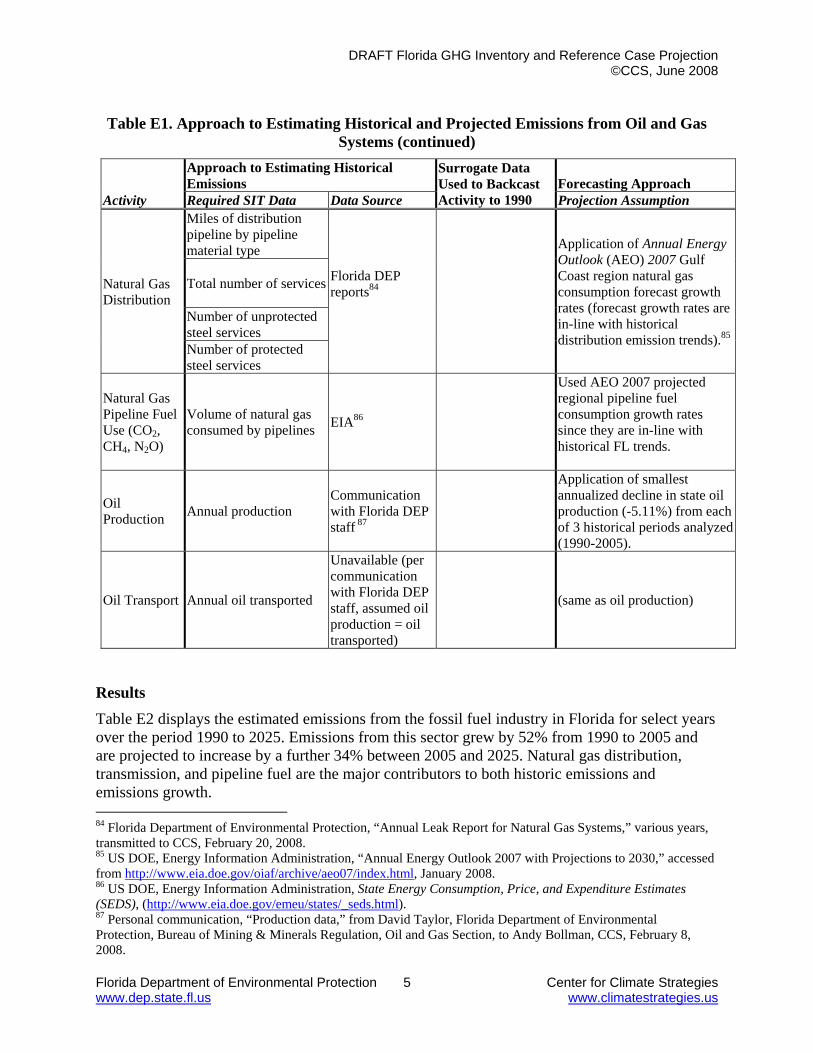
DRAFT Florida GHG Inventory and Reference Case Projection ©CCS, June 2008
Florida Department of Environmental Protection 5 Center for Climate Strategies www.dep.state.fl.us www.climatestrategies.us
Table E1. Approach to Estimating Historical and Projected Emissions from Oil and Gas
Systems (continued)
Activity
Approach to Estimating Historical Emissions
Surrogate Data Used to Backcast Activity to 1990
Forecasting Approach Required SIT Data Data Source Projection Assumption
Natural Gas Distribution
Miles of distribution pipeline by pipeline material type
Florida DEP reports84
Application of Annual Energy Outlook (AEO) 2007 Gulf Coast region natural gas consumption forecast growth rates (forecast growth rates are in-line with historical distribution emission trends).85
Total number of services
Number of unprotected steel services Number of protected steel services
Natural Gas Pipeline Fuel Use (CO2, CH4, N2O)
Volume of natural gas consumed by pipelines EIA86
Used AEO 2007 projected regional pipeline fuel consumption growth rates since they are in-line with historical FL trends.
Oil Production Annual production
Communication with Florida DEP staff 87
Application of smallest annualized decline in state oil production (-5.11%) from each of 3 historical periods analyzed(1990-2005).
Oil Transport Annual oil transported
Unavailable (per communication with Florida DEP staff, assumed oil production = oil transported)
(same as oil production)
Results Table E2 displays the estimated emissions from the fossil fuel industry in Florida for select years over the period 1990 to 2025. Emissions from this sector grew by 52% from 1990 to 2005 and are projected to increase by a further 34% between 2005 and 2025. Natural gas distribution, transmission, and pipeline fuel are the major contributors to both historic emissions and emissions growth. 84 Florida Department of Environmental Protection, “Annual Leak Report for Natural Gas Systems,” various years, transmitted to CCS, February 20, 2008. 85 US DOE, Energy Information Administration, “Annual Energy Outlook 2007 with Projections to 2030,” accessed from http://www.eia.doe.gov/oiaf/archive/aeo07/index.html, January 2008. 86 US DOE, Energy Information Administration, State Energy Consumption, Price, and Expenditure Estimates (SEDS), (http://www.eia.doe.gov/emeu/states/_seds.html). 87 Personal communication, “Production data,” from David Taylor, Florida Department of Environmental Protection, Bureau of Mining & Minerals Regulation, Oil and Gas Section, to Andy Bollman, CCS, February 8, 2008.
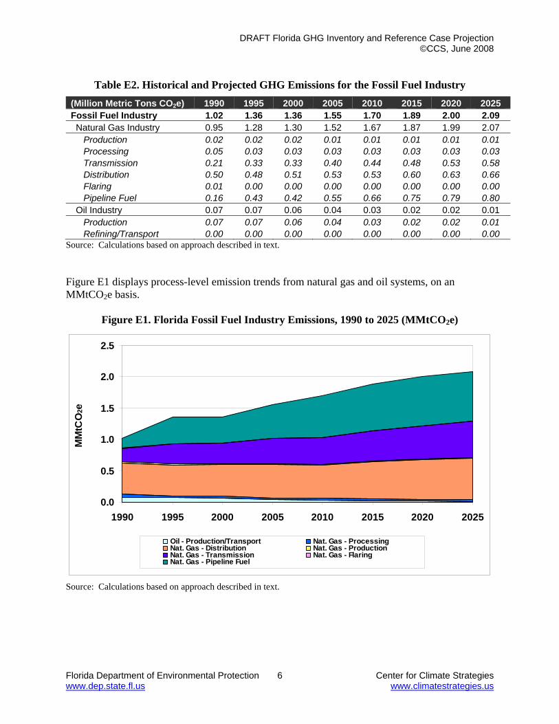
DRAFT Florida GHG Inventory and Reference Case Projection ©CCS, June 2008
Florida Department of Environmental Protection 6 Center for Climate Strategies www.dep.state.fl.us www.climatestrategies.us
Table E2. Historical and Projected GHG Emissions for the Fossil Fuel Industry
(Million Metric Tons CO2e) 1990 1995 2000 2005 2010 2015 2020 2025 Fossil Fuel Industry 1.02 1.36 1.36 1.55 1.70 1.89 2.00 2.09 Natural Gas Industry 0.95 1.28 1.30 1.52 1.67 1.87 1.99 2.07 Production 0.02 0.02 0.02 0.01 0.01 0.01 0.01 0.01 Processing 0.05 0.03 0.03 0.03 0.03 0.03 0.03 0.03 Transmission 0.21 0.33 0.33 0.40 0.44 0.48 0.53 0.58 Distribution 0.50 0.48 0.51 0.53 0.53 0.60 0.63 0.66 Flaring 0.01 0.00 0.00 0.00 0.00 0.00 0.00 0.00 Pipeline Fuel 0.16 0.43 0.42 0.55 0.66 0.75 0.79 0.80 Oil Industry 0.07 0.07 0.06 0.04 0.03 0.02 0.02 0.01 Production 0.07 0.07 0.06 0.04 0.03 0.02 0.02 0.01 Refining/Transport 0.00 0.00 0.00 0.00 0.00 0.00 0.00 0.00
Source: Calculations based on approach described in text. Figure E1 displays process-level emission trends from natural gas and oil systems, on an MMtCO2e basis.
Figure E1. Florida Fossil Fuel Industry Emissions, 1990 to 2025 (MMtCO2e)
0.0
0.5
1.0
1.5
2.0
2.5
1990 1995 2000 2005 2010 2015 2020 2025
MM
tCO
2e
Oil - Production/Transport Nat. Gas - ProcessingNat. Gas - Distribution Nat. Gas - ProductionNat. Gas - Transmission Nat. Gas - FlaringNat. Gas - Pipeline Fuel
Source: Calculations based on approach described in text.

DRAFT Florida GHG Inventory and Reference Case Projection ©CCS, June 2008
Florida Department of Environmental Protection 7 Center for Climate Strategies www.dep.state.fl.us www.climatestrategies.us
Key Uncertainties Key sources of uncertainty underlying the estimates above are as follows:
• Current levels of fugitive emissions. These are based on industry-wide averages, and until estimates are available for local facilities, significant uncertainties remain.
• Due to data limitations associated with OPS reporting, natural gas gathering and transmission pipeline emissions in earlier years were estimated by assuming that changes in each emissions producing activity were related to changes in activity levels for surrogates for the emissions activity.88
• Projections of future production of fossil fuels. The assumptions used for the projections do not reflect unknown potential future changes that could affect GHG emissions, including potential changes in regulations and emissions-reducing improvements in oil and gas production, processing, and pipeline technologies.
88 For example, gathering pipeline emissions were back-cast to pre-2001 years by applying the ratio of Florida natural gas production in each pre-2001 year to Florida natural gas production in 2001.

DRAFT Florida GHG Inventory and Reference Case Projection ©CCS, June 2008
Florida Department of Environmental Protection 1 Center for Climate Strategies www.dep.state.fl.us www.climatestrategies.us
Annex F. Agriculture Overview The emissions discussed in this Annex refer to non-energy methane (CH4) and nitrous oxide (N2O) emissions from enteric fermentation, manure management, and agricultural soils. Emissions and sinks of carbon in agricultural soils are also covered. Energy emissions (combustion of fossil fuels in agricultural equipment) are included in the residential, commercial, and industrial (RCI) sector estimates (see Annex B). There are two livestock sources of greenhouse gas (GHG) emissions: enteric fermentation and manure management. Methane emissions from enteric fermentation are the result of normal digestive processes in ruminant and non-ruminant livestock. Microbes in the animal digestive system break down food and emit CH4 as a by-product. More CH4 is produced in ruminant livestock because of digestive activity in the large fore-stomach. Methane and N2O emissions from the storage and treatment of livestock manure (e.g., in compost piles or anaerobic treatment lagoons) occur as a result of manure decomposition. The environmental conditions of decomposition drive the relative magnitude of emissions. In general, the more anaerobic the conditions are, the more CH4 is produced because decomposition is aided by CH4 producing bacteria that thrive in oxygen-limited conditions. Under aerobic conditions, N2O emissions are dominant. Emissions estimates from manure management are based on manure that is stored and treated on livestock operations. Emissions from manure that is applied to agricultural soils as an amendment or deposited directly to pasture and grazing land by grazing animals are accounted for in the agricultural soils emissions. The management of agricultural soils can result in N2O emissions and net fluxes of carbon dioxide (CO2) causing emissions or sinks. In general, soil amendments that add nitrogen to soils can also result in N2O emissions. Nitrogen additions drive underlying soil nitrification and de-nitrification cycles, which produce N2O as a by-product. The emissions estimation methodologies used in this inventory account for several sources of N2O emissions from agricultural soils, including decomposition of crop residues, synthetic and organic fertilizer application, manure application, sewage sludge, nitrogen fixation, and histosols (high organic soils, such as wetlands or peatlands) cultivation. Both direct and indirect emissions of N2O occur from the application of manure, fertilizer, and sewage sludge to agricultural soils. Direct emissions occur at the site of application and indirect emissions occur when nitrogen leaches to groundwater or in surface runoff and is transported off-site before entering the nitrification/denitrification cycle. Methane and N2O emissions also result when crop residues are burned and during rice cultivation. Rice fields must remain flooded, which means that decomposition occurs in a low-oxygen environment, resulting in anaerobic decomposition. This decomposition results in methane and N2O emissions, though total emissions can vary depending on water management practices. The net flux of CO2 in agricultural soils depends on the balance of carbon losses from management practices and gains from organic matter inputs to the soil. Carbon dioxide is absorbed by plants through photosynthesis and ultimately becomes the carbon source for organic matter inputs to agricultural soils. When inputs are greater than losses, the soil accumulates
DRAFT Florida GHG Inventory and Reference Case Projection ©CCS, June 2008
Florida Department of Environmental Protection 2 Center for Climate Strategies www.dep.state.fl.us www.climatestrategies.us
carbon and there is a net sink of CO2 into agricultural soils. In addition, soil disturbance from the cultivation of histosols releases large stores of carbon from the soil to the atmosphere. Finally, the practice of adding limestone and dolomite to agricultural soils (for neutralizing acidic soil conditions) results in CO2 emissions. Emissions and Reference Case Projections
Methane and Nitrous Oxide
GHG emissions for 1990 through 2005 were estimated using the United States Environmental Protection Agency’s (US EPA) State Greenhouse Gas Inventory Tool (SIT) software and the methods provided in the Emission Inventory Improvement Program (EIIP) guidance document for the sector.89 In general, the SIT methodology applies emission factors developed for the US to activity data for the agriculture sector. Activity data include livestock population statistics, crop production statistics, amounts of fertilizer applied to crops, and trends in manure management practices. This methodology is based on international guidelines developed by sector experts for preparing GHG emissions inventories.90 Data on crop production in Florida from 1990 to 2005 and the number of animals in the state from 1990 to 2005 were obtained from the United States Department of Agriculture (USDA) National Agriculture Statistical Service (NASS) and incorporated as defaults in SIT.91 The default SIT manure management system assumptions for each livestock category were used for this inventory. Fertilizer data for the years 1998-2005 comes from the Florida Department of Agriculture and Consumer Services, Division of Agriculture Environmental Services.92 This has data on the total nitrogen sold in the state of Florida. SIT Fertilizer data was used for 1990-1997. SIT data on fertilizer usage came from Commercial Fertilizers, a report from the Fertilizer Institute. Activity data for fertilizer includes all potential uses in addition to agriculture, such as residential and commercial (e.g., golf courses). The estimates are reported in the agriculture sector but they represent emissions occurring on other land uses. Crop production data from USDA NASS were available through 2005; therefore, N2O emissions from crop residues and crops that use nitrogen (i.e., nitrogen fixation) and N2O and CH4 emissions from agricultural residue burning were calculated through 2005. Emissions for the other agricultural crop production categories (i.e., synthetic and organic fertilizers) were also calculated through 2005. Data were not available to estimate nitrogen released by the cultivation 89 GHG emissions were calculated using SIT, with reference to EIIP, Volume VIII: Chapter 8. “Methods for Estimating Greenhouse Gas Emissions from Livestock Manure Management”, August 2004; Chapter 10. “Methods for Estimating Greenhouse Gas Emissions from Agricultural Soil Management”, August 2004; and Chapter 11. “Methods for Estimating Greenhouse Gas Emissions from Field Burning of Agricultural Residues”, August 2004. 90 Revised 1996 1ntergovermental Panel on Climate Change (IPCC) Guidelines for National Greenhouse Gas Inventories, published by the National Greenhouse Gas Inventory Program of the IPCC, available at (http://www.ipcc-nggip.iges.or.jp/public/gl/invs1.htm; and Good Practice Guidance and Uncertainty Management in National Greenhouse Gas Inventories, published in 2000 by the National Greenhouse Gas Inventory Program of the IPCC, available at: (http://www.ipcc-nggip.iges.or.jp/public/gp/english/). 91 USDA, NASS (http://www.nass.usda.gov/Statistics_by_State/florida/index.asp). 92 http://www.flaes.org/complimonitoring/reports.html Data from growing years factored together to represent calendar years, 1998-2005.

DRAFT Florida GHG Inventory and Reference Case Projection ©CCS, June 2008
Florida Department of Environmental Protection 3 Center for Climate Strategies www.dep.state.fl.us www.climatestrategies.us
of histosols (i.e., the number of acres of high organic content soils). Given that cultivation of organic soils is a source of CO2 emissions in Florida (see below), N2O emissions are also probably occurring. There is some agricultural residue burning conducted in Florida; however, emissions are estimated to be very small (~0.01 MMtCO2e). The default SIT method was used to calculate emissions. The SIT methodology calculates emissions by multiplying the amount (e.g., bushels or tons) of each crop produced by a series of factors to calculate the amount of crop residue produced and burned, the resultant dry matter, and the carbon/nitrogen content of the dry matter. Emissions from enteric fermentation and manure management were projected based on forecasted animal populations. Dairy cattle forecasts were based on state-level projections of dairy cows from the Food and Agricultural Policy Research Institute (FAPRI).93 Projections for all other livestock categories were estimated based on linear forecasts of the historical 1990-2005 populations. In the case of Swine and Broiler populations, significant population decreases occurred between 1990 and 2005, but both of these decreases seemed to level off in 2004-2005 range. Therefore, the 2005 figure was used throughout 2006-2025. Population growth rates are shown in Table F1.
Table F1. Growth Rates Applied for the Enteric Fermentation And Manure Management Categories
Livestock Category
2005-2025 Annual Growth
Dairy Cattle -2.24% Beef Cattle -0.90% Swine 0.00% Sheep 1.80% Goats 1.86% Horses -0.45% Layers 0.33% Broilers 0.00%
Projections for agricultural burning and agricultural soils were based on linear extrapolation of the 1990-2005 historical data. Table F2 shows the 2005-2025 annual growth rates estimated for each category. Crop residue values after 2005 were held at 2005 levels to prevent a forecast of negative emissions. SIT defaults for rice cultivation are derived from the US Agriculture and Forestry Greenhouse Gas Inventory.94 Projections for rice cultivation were held constant at 2005 levels.
93 FAPRI Agricultural Outlook 2006, Food and Agricultural Policy Research Institute, http://www.fapri.iastate.edu/outlook2006. 94 USDA, published March 2004. Accessed at http://www.usda.gov/oce/global_change/gg_inventory.htm, Feb, 2008. See Appendix B, Table B-6.
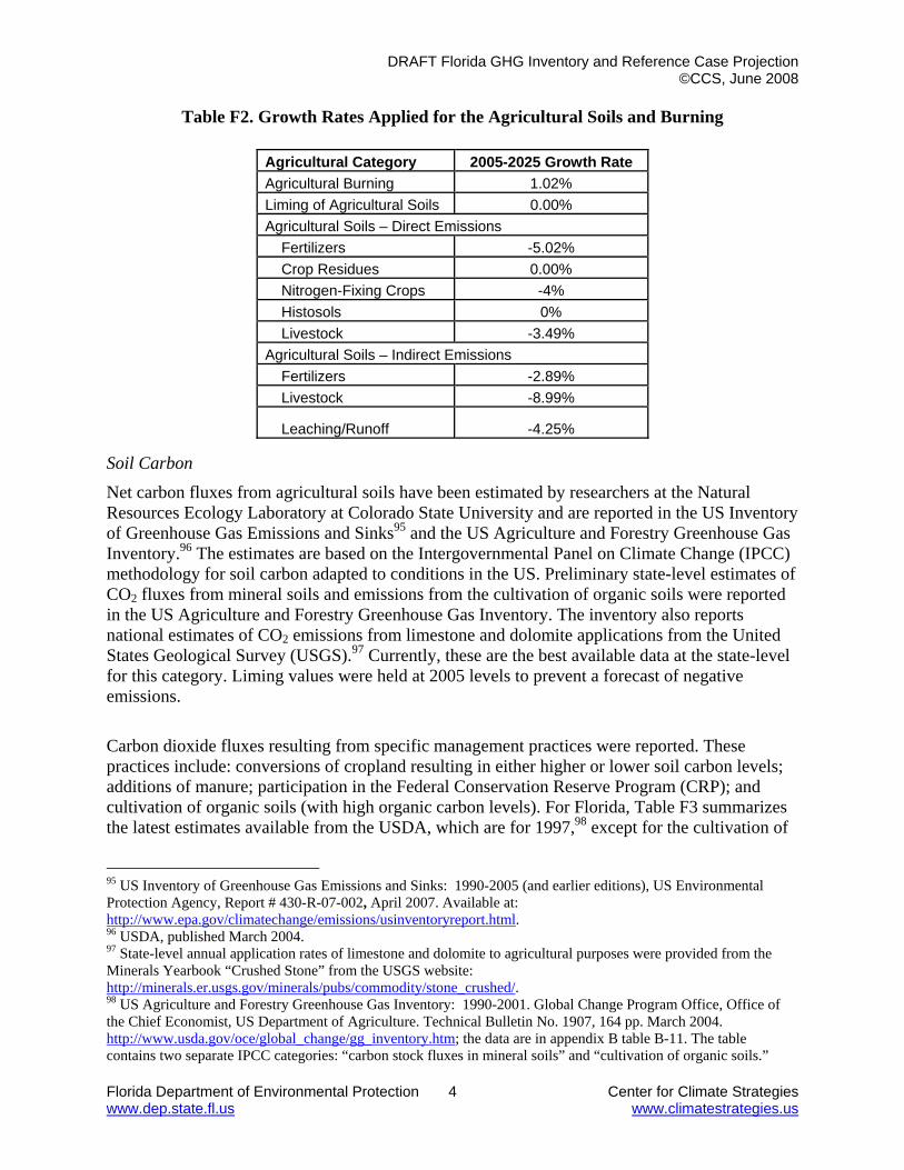
DRAFT Florida GHG Inventory and Reference Case Projection ©CCS, June 2008
Florida Department of Environmental Protection 4 Center for Climate Strategies www.dep.state.fl.us www.climatestrategies.us
Table F2. Growth Rates Applied for the Agricultural Soils and Burning
Agricultural Category 2005-2025 Growth Rate Agricultural Burning 1.02% Liming of Agricultural Soils 0.00% Agricultural Soils – Direct Emissions Fertilizers -5.02% Crop Residues 0.00% Nitrogen-Fixing Crops -4% Histosols 0% Livestock -3.49% Agricultural Soils – Indirect Emissions Fertilizers -2.89% Livestock -8.99%
Leaching/Runoff -4.25% Soil Carbon
Net carbon fluxes from agricultural soils have been estimated by researchers at the Natural Resources Ecology Laboratory at Colorado State University and are reported in the US Inventory of Greenhouse Gas Emissions and Sinks95 and the US Agriculture and Forestry Greenhouse Gas Inventory.96 The estimates are based on the Intergovernmental Panel on Climate Change (IPCC) methodology for soil carbon adapted to conditions in the US. Preliminary state-level estimates of CO2 fluxes from mineral soils and emissions from the cultivation of organic soils were reported in the US Agriculture and Forestry Greenhouse Gas Inventory. The inventory also reports national estimates of CO2 emissions from limestone and dolomite applications from the United States Geological Survey (USGS).97 Currently, these are the best available data at the state-level for this category. Liming values were held at 2005 levels to prevent a forecast of negative emissions.
Carbon dioxide fluxes resulting from specific management practices were reported. These practices include: conversions of cropland resulting in either higher or lower soil carbon levels; additions of manure; participation in the Federal Conservation Reserve Program (CRP); and cultivation of organic soils (with high organic carbon levels). For Florida, Table F3 summarizes the latest estimates available from the USDA, which are for 1997,98 except for the cultivation of
95 US Inventory of Greenhouse Gas Emissions and Sinks: 1990-2005 (and earlier editions), US Environmental Protection Agency, Report # 430-R-07-002, April 2007. Available at: http://www.epa.gov/climatechange/emissions/usinventoryreport.html. 96 USDA, published March 2004. 97 State-level annual application rates of limestone and dolomite to agricultural purposes were provided from the Minerals Yearbook “Crushed Stone” from the USGS website: http://minerals.er.usgs.gov/minerals/pubs/commodity/stone_crushed/. 98 US Agriculture and Forestry Greenhouse Gas Inventory: 1990-2001. Global Change Program Office, Office of the Chief Economist, US Department of Agriculture. Technical Bulletin No. 1907, 164 pp. March 2004. http://www.usda.gov/oce/global_change/gg_inventory.htm; the data are in appendix B table B-11. The table contains two separate IPCC categories: “carbon stock fluxes in mineral soils” and “cultivation of organic soils.”

DRAFT Florida GHG Inventory and Reference Case Projection ©CCS, June 2008
Florida Department of Environmental Protection 5 Center for Climate Strategies www.dep.state.fl.us www.climatestrategies.us
organic soils, which is based on a University of Florida report on soil carbon.99 These data show that changes in agricultural practices are estimated to result in net emissions of 9.63 million metric tons (MMt) of CO2 equivalent (CO2e) per year in Florida; this is driven largely by the cultivation of organic soils in Florida. Since updated data are not yet available from USDA to make a determination of whether the emissions are increasing or decreasing, emissions of 9.63 MMtCO2e per year are assumed to remain constant. Note that emissions from agricultural soils estimated using the SIT were multiplied by a national adjustment factor to reconcile differences between methodologies used in the National Inventory of Greenhouse Gas Emissions and the SIT.
Table F3. GHG Emissions from Soil Carbon Changes Due to Cultivation Practices
(MMtCO2e) Changes in cropland Changes in Hayland Other Total5
Plowout of
grassland to annual cropland1
Cropland manage-
ment Other
cropland2
Cropland converted
to hayland3
Hayland manage-
ment
Cropland converted to grazing
land3
Grazing land
manage-ment CRP
Manure application
Cultivation of organic
soils4
Net soil carbon
emissions 0.33 (0.04) (0.22) (0.07) 0.00 (0.48) 0.11 (0.07) (0.23) 10.30 9.63
Based on USDA 1997 estimates, except where noted. Parentheses indicate net sequestration. 1 Losses from annual cropping systems due to plow-out of pastures, rangeland, hayland, set-aside lands, and perennial/horticultural cropland (annual cropping systems on mineral soils, e.g., corn, soybean, cotton, and wheat). 2 Perennial/horticultural cropland and rice cultivation. 3 Gains in soil carbon sequestration due to land conversions from annual cropland into hay or grazing land. 4 Based on University of Florida report “Opportunities for Greenhouse Gas Reduction Through Forestry and Agriculture in Florida” as mentioned in text. 5 Total does not include change in soil organic carbon storage on federal lands, including those that were previously under private ownership, and does not include carbon storage due to sewage sludge applications.
Results Figure F1 and Table F4 show gross GHG emissions associated with the agricultural sector from 1990 through 2025. Cultivation of soils is estimated to be the largest source of net emissions source in Florida. The emissions for this category are estimated to account for 59% of total agricultural emissions in 1990 and about 73% of total emissions in 2025. Since data are not yet available from USDA to determine if emissions are increasing or decreasing, emissions of 9.63 MMtCO2e per year are assumed to remain constant throughout the inventory and forecast period. The percentage of emissions from cultivation of soils is increasing because other agricultural emissions sources are estimated to decrease between 1990 and 2025. The latter is shown in the second to last column of Table F3. The sum of the first nine columns is equivalent to the mineral soils category. 99 “Opportunities for Greenhouse Gas Reduction Through Forestry and Agriculture in Florida”, University of Florida School of Natural Resources and Environment, April 2008, Stephen Mulkey, et al, see page 44 of chapter: “Role of Florida soils in carbon sequestration” by Sabine Grunwald. Report can be downloaded at http://snre.ufl.edu/pubsevents/source/summer08/climatereport.htm, accessed July 2008.
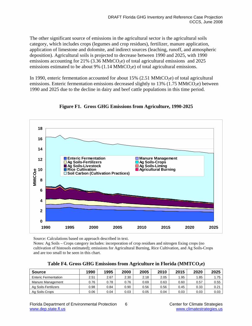
DRAFT Florida GHG Inventory and Reference Case Projection ©CCS, June 2008
Florida Department of Environmental Protection 6 Center for Climate Strategies www.dep.state.fl.us www.climatestrategies.us
The other significant source of emissions in the agricultural sector is the agricultural soils category, which includes crops (legumes and crop residues), fertilizer, manure application, application of limestone and dolomite, and indirect sources (leaching, runoff, and atmospheric deposition). Agricultural soils is projected to decrease between 1990 and 2025, with 1990 emissions accounting for 21% (3.36 MMtCO2e) of total agricultural emissions and 2025 emissions estimated to be about 9% (1.14 MMtCO2e) of total agricultural emissions. In 1990, enteric fermentation accounted for about 15% (2.51 MMtCO2e) of total agricultural emissions. Enteric fermentation emissions decreased slightly to 13% (1.75 MMtCO2e) between 1990 and 2025 due to the decline in dairy and beef cattle populations in this time period.
Figure F1. Gross GHG Emissions from Agriculture, 1990-2025
0
2
4
6
8
10
12
14
16
18
1990 1995 2000 2005 2010 2015 2020 2025
MM
tCO 2
e
Enteric Fermentation Manure ManagementAg Soils-Fertilizers Ag Soils-CropsAg Soils-Livestock Ag Soils-LimingRice Cultivation Agricultural BurningSoil Carbon (Cultivation Practices)
Source: Calculations based on approach described in text. Notes: Ag Soils – Crops category includes: incorporation of crop residues and nitrogen fixing crops (no cultivation of histosols estimated); emissions for Agricultural Burning, Rice Cultivation, and Ag Soils-Crops and are too small to be seen in this chart.
Table F4. Gross GHG Emissions from Agriculture in Florida (MMTCO2e)
Source 1990 1995 2000 2005 2010 2015 2020 2025Enteric Fermentation 2.51 2.67 2.30 2.18 2.05 1.95 1.85 1.75 Manure Management 0.76 0.78 0.76 0.69 0.63 0.60 0.57 0.55 Ag Soils-Fertilizers 0.98 0.84 0.90 0.56 0.56 0.45 0.33 0.21 Ag Soils-Crops 0.06 0.04 0.03 0.05 0.04 0.03 0.03 0.03
DRAFT Florida GHG Inventory and Reference Case Projection ©CCS, June 2008
Florida Department of Environmental Protection 7 Center for Climate Strategies www.dep.state.fl.us www.climatestrategies.us
Ag Soils-Livestock 1.97 1.85 1.57 1.67 1.28 1.10 0.93 0.75 Ag Soils-Liming 0.35 0.24 0.23 0.15 0.15 0.15 0.15 0.15 Rice Cultivation 0.06 0.12 0.09 0.06 0.06 0.06 0.06 0.06 Agricultural Burning 0.01 0.01 0.01 0.01 0.01 0.01 0.01 0.01 Soil Carbon (Cultivation Practices) 9.63 9.63 9.63 9.63 9.63 9.63 9.63 9.63 TOTAL 16.33 16.17 15.51 15.00 14.42 13.98 13.56 13.14
The manure management category accounted for 5% (0.76 MMtCO2e) of total agricultural emissions in 1990 and decreased slightly over the next thirty five years, accounting for 4% (0.55 MMtCO2e) in 2025. This is largely due to the projection that the dairy cow population will decrease between 1990 and 2025. Rice cultivation accounted for less than 1% (0.06 MMtCO2e) of agricultural emissions in 1990 and in 2005 and is projected to remain steady throughout the forecast period. The only standard IPCC source category missing from this report is N2O emissions from the cultivation of histosols; there was no activity data available for Florida.
Key Uncertainties Emissions from enteric fermentation and manure management are dependent on the estimates of animal populations and the various factors used to estimate emissions for each animal type and manure management system (i.e., emission factors which are derived from several variables including manure production levels, volatile solids content, and CH4 formation potential). Each of these factors has some level of uncertainty. Also, animal populations fluctuate throughout the year, and thus using point estimates introduces uncertainty into the average annual estimates of these populations. In addition, there is uncertainty associated with the original population survey methods employed by USDA. The largest contributors to uncertainty in emissions from manure management are the emission factors, which are derived from limited data sets. As mentioned above, the USDA estimates for emissions associated with changes in agricultural soil carbon levels are from 1997. Newer data are scheduled to be released by the USDA by August 2008. When released, the data should be reviewed to represent current conditions as well as to assess trends. In particular, given the potential for some CRP acreage to retire and possibly return to active cultivation prior to 2025, the emissions could be appreciably affected. The data on cultivation of histosol soils will be compared to that reported by Dr. Sabine Grunwald in the University of Florida study. Uncertainties in the estimates of emissions from liming result from both the emission factors and the activity data. It is uncertain what fraction of agricultural lime is dissolved by nitric acid – a process that releases CO2 – and what portion reacts with carbonic acid (H2CO3), resulting in the uptake of CO2. Also, there is uncertainty in the limestone and dolomite data (reported to USGS) as some producers do not distinguish between them, and report them both as limestone. Another contributor to the uncertainty in the emission estimates is the forecast assumptions. The growth rates for most categories are assumed to continue growing at historical 1990-2005 growth
DRAFT Florida GHG Inventory and Reference Case Projection ©CCS, June 2008
Florida Department of Environmental Protection 8 Center for Climate Strategies www.dep.state.fl.us www.climatestrategies.us
rates. These historic trends may not reflect future projections. Other emissions are assumed to remain at 2004-2005 levels (as noted under Emissions and Reference Case Projections) to prevent a forecast of negative emissions for those categories.

DRAFT Florida GHG Inventory and Reference Case Projection ©CCS, June 2008
Florida Department of Environmental Protection 1 Center for Climate Strategies www.dep.state.fl.us www.climatestrategies.us
Annex G. Waste Management
Overview Greenhouse gas (GHG) emissions from waste management include:
• Solid waste management – methane (CH4) emissions from municipal and industrial solid waste landfills (LFs), accounting for CH4 that is flared or captured for energy production (this includes both open and closed landfills)100;
• Solid waste combustion – CH4, carbon dioxide (CO2), and nitrous oxide (N2O) emissions from the combustion of solid waste in incinerators or at open residential sites (i.e. backyard burn barrels); and
• Wastewater management – CH4 and N2O from municipal wastewater (WW) and CH4 from industrial wastewater treatment facilities.
Inventory and Reference Case Projections
Solid Waste Management
For solid waste management, the United States Environmental Protection Agency’s (US EPA) State Inventory Tool (SIT) software was used to estimate emissions. Activity data relating to waste managed in landfill facilities was obtained from U.S. EPA's Landfill Methane Outreach Program (LMOP). Supplemental landfill facilities information was provided by staff of the Department of Environmental Protection (DEP), Solid Waste Section, from state level historical and current databases. In order to run SIT’s emissions model, substantial gaps in activity data were filled in with average values as follows:
a) Waste in place, 4,503,323 tons b) Year waste in place was measured, 2000 c) Year landfill opened, 1977 d) Year landfill closed, 2006
DEP databases also signaled the existence of approximately 270 more Class I and II MSW landfills (mostly closed) in addition to the 133 sites listed on the LMOP summary.101 DEP staff qualified these additional sites as older and smaller with decreased or no gas generation.102 Moreover, CCS did not apply the default SIT assumption that 10% of CH4 is oxidized as it travels through the surface layers of the landfill due to a lack of information to support this assumption. Another assumption factored into the emissions estimate was the methane capture rate of landfill-gas-to-energy (LFGTE) sites and sites where flaring occurs. Both were assumed to have a methane capture rate of 75%, the remaining fraction deemed to be methane fugitive emissions.
100 CCS acknowledges that N2O and CH4 emissions are also produced from the combustion of landfill gas; however, these emissions tend to be negligible for the purposes of developing a state-level inventory for policy analysis. 101 Retrieved from http://www.epa.gov/landfill/ 102 Based on e-mail correspondence between Mr. Lee Martin (DEP) and Dr. Rachel Anderson (CCS) dated 1/29/08.
DRAFT Florida GHG Inventory and Reference Case Projection ©CCS, June 2008
Florida Department of Environmental Protection 2 Center for Climate Strategies www.dep.state.fl.us www.climatestrategies.us
Emissions for industrial solid waste landfills were estimated using the SIT default activity data and emission factors. The activity data are based on national data indicating that industrial landfill methane emissions are approximately 7% of total municipal solid waste (MSW) emissions nationally. Finally, solid waste management emissions results were consolidated into five groups. Growth rates were estimated by using the historical (2000-2005) growth rates of each group as shown on Table G1
Table G1. MSW Emissions Grouping and Growth Rates
Emissions Grouping Case Projection Growth Rate MSW LFGTE 0.80% MSW Flared 2.94% MSW Uncontrolled 2.05% MSW Uncontrolled & closed over 15 year -3.92% Industrial LFs 1.68%
Solid Waste Combustion
Sources of solid waste combustion include municipal solid waste (MSW) combustors, medical waste incinerators, and residential open burning. Emissions from municipal solid waste-to-energy combustors, of which Florida has twelve, are not inventoried here but are included in the energy supply sector inventory. Quantities of medical waste incinerated were obtained from Florida DEP.103 The historical (1995-2005) growth rate of -1.7% for medical waste incineration was used to estimate future growth rates. Open burning of MSW at residential sites (e.g. backyard burn barrels) was estimated using the US EPA’s 2002 National Emissions Inventory (NEI) methodology for calculating the quantity of waste burned at residential sites in Florida.104 Emissions from open burning were calculated using SIT emission factors and waste characteristics. The historical (1990-2005) growth rate of -1.7% for residential waste burning was used to estimate future growth rates. Wastewater Management
GHG emissions from municipal wastewater treatment were also estimated. For municipal WW treatment, emissions are calculated in EPA’s SIT based on state population, assumed biochemical oxygen demand (BOD) and protein consumption per capita, and emission factors for N2O and CH4. The key SIT default values are shown in Table G1 below. Municipal wastewater emissions were projected based on the historical growth rate for 1990-2005 of 2.3% per year.
103 Yi Zhu, Florida Department of Environmental Protection, communicated via email to Rachel Anderson, CCS, March 6, 2008. 104 EPA, ftp://ftp.epa.gov/EmisInventory/2002finalnei/documentation/nonpoint/2002nei_final_nonpoint_documentation0206version.pdf.
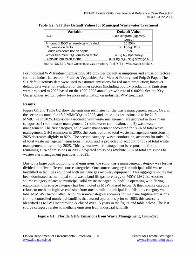
DRAFT Florida GHG Inventory and Reference Case Projection ©CCS, June 2008
Florida Department of Environmental Protection 3 Center for Climate Strategies www.dep.state.fl.us www.climatestrategies.us
Table G2. SIT Key Default Values for Municipal Wastewater Treatment
Variable Default Value BOD 0.09 kilogram (kg) /day-
person Amount of BOD anaerobically treated 16.25% CH4 emission factor 0.6 kg/kg BOD Florida residents not on septic 75%Water treatment N2O emission factor 4.0 g N2O/person-yr Biosolids emission factor 0.01 kg N2O-N/kg sewage-N
Source: US EPA State Greenhouse Gas Inventory Tool (SIT) – Wastewater Module. For industrial WW treatment emissions, SIT provides default assumptions and emission factors for three industrial sectors: Fruits & Vegetables, Red Meat & Poultry, and Pulp & Paper. The SIT default activity data were used to estimate emissions for red meat production; however, default data were not available for the other sectors (including poultry production). Emissions were projected to 2025 based on the 1990-2005 annual growth rate of 0.002%. See the Key Uncertainties section below for more information on industrial WW treatment. Results Figure G1 and Table G2 show the emission estimates for the waste management sector. Overall, the sector accounts for 15.3 MMtCO2e in 2005, and emissions are estimated to be 21.9 MMtCO2e in 2025. Emissions associated with waste management are grouped in three main categories: 1) solid waste management, 2) solid waste combustion, and 3) wastewater management. The first category, solid waste management accounted for 83% of total waste management GHG emissions in 2005; the contribution to total waste management emissions in 2025 decreases slightly to 82%. The second category, waste combustion, accounts for only 1% of total waste management emissions in 2005 and is projected to account for 1% of total waste management emission by 2025. Thirdly, wastewater management is responsible for the remaining 16% of emissions in 2005; projected emissions attribute 17% of total emissions to wastewater management practices in 2025. Due to its large contribution to total emissions, the solid waste management category was further divided into five different source categories. One source category is municipal solid waste landfilled in facilities equipped with methane gas recovery equipment. This aggregate source has been dominated as municipal solid waste land fill gas-to-energy or MSW LFGTE. Another source category relates to municipal solid waste managed in landfills operating with flaring equipment; this source category has been noted as MSW Flared below. A third source category relates to methane fugitive emission from uncontrolled municipal landfills; this category was labeled MSW Uncontrolled. A fourth source category accounts for methane fugitive emissions from uncontrolled municipal landfills that ceased operations prior to 1983; this source is identified as MSW Uncontrolled & closed over 15 years in the figure and table below. The last source category relates to methane emission from industrial landfills.
Figure G1. Florida GHG Emissions from Waste Management, 1990-2025
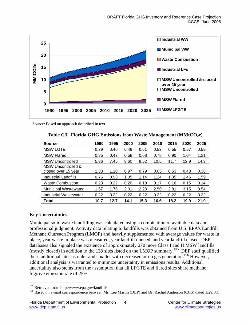
DRAFT Florida GHG Inventory and Reference Case Projection ©CCS, June 2008
Florida Department of Environmental Protection 4 Center for Climate Strategies www.dep.state.fl.us www.climatestrategies.us
0
5
10
15
20
25
1990 1995 2000 2005 2010 2015 2020 2025
MM
tCO
2eIndustrial WW
Municipal WW
Waste Combustion
Industrial LFs
MSW Uncontrolled & closedover 15 yearMSW Uncontrolled
MSW Flared
MSW LFGTE
Source: Based on approach described in text.
Table G3. Florida GHG Emissions from Waste Management (MMtCO2e)
Source 1990 1995 2000 2005 2010 2015 2020 2025 MSW LGTE 0.39 0.46 0.49 0.51 0.53 0.55 0.57 0.59 MSW Flared 0.35 0.47 0.58 0.68 0.78 0.90 1.04 1.21 MSW Uncontrolled 5.86 7.45 8.60 9.52 10.5 11.7 12.9 14.3 MSW Uncontrolled & closed over 15 year 1.33 1.18 0.97 0.79 0.65 0.53 0.43 0.36 Industrial Landfills 0.76 0.93 1.05 1.14 1.24 1.35 1.46 1.59 Waste Combustion 0.23 0.22 0.20 0.19 0.17 0.16 0.15 0.14 Municipal Wastewater 1.57 1.75 2.01 2.23 2.50 2.81 3.15 3.54 Industrial Wastewater 0.22 0.22 0.22 0.22 0.22 0.22 0.22 0.22 Total 10.7 12.7 14.1 15.3 16.6 18.2 19.9 21.9
Key Uncertainties Municipal solid waste landfilling was calculated using a combination of available data and professional judgment. Activity data relating to landfills was obtained from U.S. EPA's Landfill Methane Outreach Program (LMOP) and heavily supplemented with average values for waste in place, year waste in place was measured, year landfill opened, and year landfill closed. DEP databases also signaled the existence of approximately 270 more Class I and II MSW landfills (mostly closed) in addition to the 133 sites listed on the LMOP summary.105 DEP staff qualified these additional sites as older and smaller with decreased or no gas generation.106 However, additional analysis is warranted to minimize uncertainty in emissions results. Additional uncertainty also stems from the assumption that all LFGTE and flared sites share methane fugitive emission rate of 25%.
105 Retrieved from http://www.epa.gov/landfill/ 106 Based on e-mail correspondence between Mr. Lee Martin (DEP) and Dr. Rachel Anderson (CCS) dated 1/29/08.

DRAFT Florida GHG Inventory and Reference Case Projection ©CCS, June 2008
Florida Department of Environmental Protection 5 Center for Climate Strategies www.dep.state.fl.us www.climatestrategies.us
For industrial landfills, emissions were estimated using national defaults (with industrial landfill emissions approximately 7% of MSW emissions). Depending on actual industrial landfill emissions in Florida, this could be an over- or underestimate. SIT MSW defaults including waste composition and emissions factors were used to estimate medical waste incineration emissions in FL. To the extent that the fossil carbon content of medical waste differs from municipal solid waste, this could be an over- or underestimate. Open burning of waste at residential sites was estimated using a US EPA NEI methodology. Depending on actual burn rates, this could be an over- or underestimate. Emissions from open burning of yard waste were not estimated but are expected to be small (only the CH4 and N2O emissions would be of interest here, since the CO2 would be considered to be biogenic).
For the municipal WW treatment sector, the key uncertainties are associated with the application of SIT default values for the parameters listed in Table G1 above (e.g. fraction of the Florida population on septic; fraction of BOD which is anaerobically decomposed). The SIT defaults were derived from national data. For industrial WW treatment, emissions were only estimated for the red meat industry using default data; default data for fruits and vegetables, poultry, and pulp and paper were not available. Therefore, emissions from industrial WW treatment are likely to be underestimated. This inventory in its current state does not quantify current actions taken by the State of Florida that may lower future emissions. CCS is not aware of any current actions that would have an impact on the emissions forecast.

FINAL Florida GHG Inventory and Reference Case Projection ©CCS, October 2008
Florida Department of Environmental Protection 1 Center for Climate Strategies www.dep.state.fl.us www.climatestrategies.us
Annex H. Forestry & Land Use
Overview Forestry emissions refer to the net carbon dioxide (CO2) flux107 from forested lands in Florida, which account for about 47% of the state’s land area.108 The dominant forest type in Florida is Longleaf-slash pine which makes up about 35% of forested lands. Other common forest types are Oak-gum-cypress at 18%, Oak-hickory at 17%, Loblolly-shortleaf at 9%, and Oak-pine at 9% of forested land. All other forest types make up less than 4% each of the State’s forests. Through photosynthesis, CO2 is taken up by trees and plants and converted to carbon in biomass within the forests. Carbon dioxide emissions occur from respiration in live trees, decay of dead biomass, and combustion (both wildland fires and biomass removed from forests for energy use). In addition, carbon is stored for long time periods when forest biomass is harvested for use in durable wood products. Carbon dioxide flux is the net balance of CO2 removals from and emissions to the atmosphere from the processes described above. The forestry sector net GHG emissions are categorized into two primary subsectors:
• Forested Landscape: this consists of carbon flux occurring on lands that are not part of the urban landscape. Fluxes covered include net carbon sequestration, carbon stored in harvested wood products (HWP) or landfills, and emissions from forest fires.
• Urban Forestry and Land Use: this covers carbon sequestration in urban trees, carbon flux associated with carbon storage from landscape waste and food scraps in landfills, and nitrous oxide (N2O) emissions from settlement soils (those occurring as a result of application of synthetic fertilizers in urbanized areas).
Inventory and Reference Case Projections
Forested Landscape
For over a decade, the United States Forest Service (USFS) has been developing and refining a forest carbon modeling system for the purposes of estimating forest carbon inventories. The methodology is used to develop national forest CO2 fluxes for the official US Inventory of Greenhouse Gas Emissions and Sinks. The national estimates are compiled from state-level data. The Florida forest CO2 flux data in this report come from the national analysis and are provided by the USFS. See the footnotes below for the most current documentation for the forest carbon modeling.109 Additional forest carbon information is in the form of specific carbon conversion factors.110
107 “Flux” refers to both emissions of CO2 to the atmosphere and removal (sinks) of CO2 from the atmosphere. 108 Total forested acreage is 16.1 million acres in 2005. Acreage by forest type available from USFS Southern Research Station report, Florida’s Forests – 2005 Update at: http://www.treesearch.fs.fed.us/pubs/28996. The total land area in Florida is 34.6 million acres (http://www.50states.com/Florida.htm). 109 The most current citation for an overview of how the USFS calculates the inventory based forest carbon estimates as well as carbon in harvested wood products is from the US Inventory of Greenhouse Gas Emissions and Sinks: 1990-2005 (and earlier editions), US Environmental Protection Agency, Report # USEPA #430-R-07-002, April 2007, available at: http://epa.gov/climatechange/emissions/usinventoryreport.html. Both Appendix 3.12 and Chapter 7 LULUCF are useful sources of reference. See also Smith, J.E., L.S. Heath, and M.C. Nichols (in press), US Forest

FINAL Florida GHG Inventory and Reference Case Projection ©CCS, October 2008
Florida Department of Environmental Protection 2 Center for Climate Strategies www.dep.state.fl.us www.climatestrategies.us
The forest CO2 flux methodology relies on input data in the form of plot-level forest volume statistics from the Forest Inventory and Analysis (FIA) Program. FIA data on forest volumes are converted to values for ecosystem carbon stocks (i.e., the amount of carbon stored in forest carbon pools) using the FORCARB2 modeling system. Coefficients from FORCARB2 are applied to the plot level survey data to give estimates of C density [megagrams (Mg) per hectare] for a number of separate C pools (see Table H1 for Florida C pools). Additional background on the FORCARB system is provided in a number of publications.111 Carbon dioxide flux is estimated as the change in carbon mass for each carbon pool over a specified time-frame. Forest biomass data from at least two points in time are required. The change in carbon stocks between time intervals is estimated for specific carbon pools (Live Tree, Standing Dead Wood, Understory, Down & Dead Wood, Forest Floor, and Soil Organic Carbon) and divided by the number of years between inventory samples. Annual increases in carbon density reflect carbon sequestration in a specific pool; decreases in carbon density reveal CO2 emissions or carbon transfers out of that pool (e.g., death of a standing tree transfers carbon from the live tree to standing dead wood pool). The amount of carbon in each pool is also influenced by changes in forest area (e.g., an increase in area could lead to an increase in the associated forest carbon pools and the estimated flux). The sum of carbon stock changes for all forest carbon pools yields a total net CO2 flux for forest ecosystems. In preparing these estimates, USFS estimates the amount of forest carbon in different forest types as well as different carbon pools. The different forests also include differences in ownership class: those in the national forest (NF) system and those that are not federally-owned (private and other public forests). Additional details on the forest carbon inventory methods can be found in Annex 3 to the US EPA’s 2007 GHG inventory for the US.112 Carbon pool data for three FIA cycles to estimate flux for two different periods were available for Florida. The carbon pool data for three points in time are shown in Table H1 below. Note that prior to 1995, the Southern FIA Program took periodic forest inventory surveys for Florida (approximately on a 10-year schedule). Beginning in 2001, Florida transitioned from periodic to annual inventories as modifications to the FIA program were applied. The annual inventory is expected to measure 20 percent of the plots in Florida each year, and delivers a complete inventory report every 5 years. The 2005 inventory, however, only covers 60 percent of all Carbon Calculation Tool User’s Guide: Forestland Carbon Stocks and Net Annual Stock Change, Gen Tech Report, Newtown Square, PA: US Department of Agriculture, Forest Service, Northern Research Station. 110 Smith, J.E., and L.S. Heath (2002). “A model of forest floor carbon mass for United States forest types,” Res. Pap. NE-722. Newtown Square, PA: US Department of Agriculture, Forest Service, Northeastern Research Station. 37 p., or Jenkins, J.C., D.C. Chojnacky, L.S. Heath, R.A. Birdsey (2003), “National-scale biomass estimators for United States tree species”, Forest Science, 49:12-35. 111 Smith, J.E., L.S. Heath, and P.B. Woodbury (2004). “How to estimate forest carbon for large areas from inventory data”, Journal of Forestry, 102: 25-31; Heath, L.S., J.E. Smith, and R.A. Birdsey (2003), “Carbon trends in US forest lands: A context for the role of soils in forest carbon sequestration”, In J. M. Kimble, L. S. Heath, R. A. Birdsey, and R. Lal, editors. The Potential of US Forest Soils to Sequester Carbon and Mitigate the Greenhouse Effect. CRC Press, New York; and Woodbury, Peter B.; Smith, James E.; Heath, Linda S. 2007, “Carbon sequestration in the US forest sector from 1990 to 2010”, Forest Ecology and Management, 241:14-27. 112 Annex 3 to EPA’s 2007 report, which contains estimates for calendar year 2005, can be downloaded at: http://www.epa.gov/climatechange/emissions/downloads06/07Annex3.pdf.

FINAL Florida GHG Inventory and Reference Case Projection ©CCS, October 2008
Florida Department of Environmental Protection 3 Center for Climate Strategies www.dep.state.fl.us www.climatestrategies.us
sample plots in the State, due to a slower start of the annual inventory program. According to USFS, 20 percent of the sample plots were scheduled to be completed annually after 2005. These underlying FIA data, as shown in Table H1, display a net decrease of 402,000 acres in forested area between 1987 and 2005. Between 1987 and 1995, forested area decreased 328 thousand acres; forested area decreased an additional 74 thousand acres from 1995 to 2005. Most of the forested lands in Florida are considered timberland, meaning they are unreserved productive forestland producing, or capable of producing, crops of industrial wood. The timberland area is shown to have decreased by 332 thousand acres between 1987 and 1995 while it increased 901 thousand acres between 1995 and 2005. This increase in timberland area kept total carbon levels in 2005 (1,100 million metric tons) similar to the carbon level in 1987 (1,116 million metric tons) despite overall forest area decreases. It is not clear based on currently available information how much of this growth in timberland area is due to methodological changes (see Key Uncertainties section below) or land use conversion (e.g. agricultural use to forested use).
Table H1. USFS Forest Carbon Pool Data for Florida
Forest Pool 1987 (MMtC) Adjusted 1995 (MMtC) 2005 (MMtC)
Live Tree – Above Ground 241.9 241.5 274.9
Live Tree – Below Ground 48.9 48.9 55.4
Understory 21.1 21.1 20.5 Standing Dead 11.4 11.4 11.1 Down Dead 19.0 19.2 22.2 Forest Floor 51.4 50.6 51.5 Soil Carbon 722.4 676.7 664.2
Totals 1,116 1,069 1,100
Forest Area 1987 (103 acres)
1995 (103 acres)
2005 (103 acres)
All Forests 16,549 16,221 16,147 Timberland 14,983 14,651 15,552
MMtC = million metric tons of carbon. Positive numbers indicate net emission. Multiply MMtC by 3.67 (44/12) to convert to MMtCO2. Totals may not sum exactly due to independent rounding. Data source: Smith, James, et al. US Forest Carbon Calculation Tool: Forest-Land Carbon Stocks and Net Annual Stock Change (http://www.nrs.fs.fed.us/pubs/2394), December 2007. Adjusted for 1995 total Forest Area: Brown, Mark, J. Florida’s Forests – 2005 Update (http://www.treesearch.fs.fed.us/pubs/28996), June 2008.
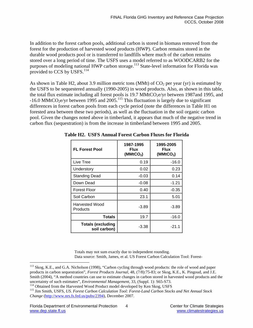
FINAL Florida GHG Inventory and Reference Case Projection ©CCS, October 2008
Florida Department of Environmental Protection 4 Center for Climate Strategies www.dep.state.fl.us www.climatestrategies.us
In addition to the forest carbon pools, additional carbon is stored in biomass removed from the forest for the production of harvested wood products (HWP). Carbon remains stored in the durable wood products pool or is transferred to landfills where much of the carbon remains stored over a long period of time. The USFS uses a model referred to as WOODCARB2 for the purposes of modeling national HWP carbon storage.113 State-level information for Florida was provided to CCS by USFS.114 As shown in Table H2, about 3.9 million metric tons (MMt) of CO2 per year (yr) is estimated by the USFS to be sequestered annually (1990-2005) in wood products. Also, as shown in this table, the total flux estimate including all forest pools is 19.7 MMtCO2e/yr between 1987and 1995, and -16.0 MMtCO2e/yr between 1995 and 2005.115 This fluctuation is largely due to significant differences in forest carbon pools from each cycle period (note the differences in Table H1 on forested area between these two periods), as well as the fluctuation in the soil organic carbon pool. Given the changes noted above in timberland, it appears that much of the negative trend in carbon flux (sequestration) is from the increase in timberland between 1995 and 2005.
Table H2. USFS Annual Forest Carbon Fluxes for Florida
FL Forest Pool 1987-1995
Flux (MMtCO2)
1995-2005 Flux
(MMtCO2)
Live Tree 0.19 -16.0
Understory 0.02 0.23
Standing Dead -0.03 0.14
Down Dead -0.08 -1.21
Forest Floor 0.40 -0.35
Soil Carbon 23.1 5.01
Harvested Wood Products -3.89 -3.89
Totals 19.7 -16.0
Totals (excluding soil carbon) -3.38 -21.1
Totals may not sum exactly due to independent rounding. Data source: Smith, James, et al. US Forest Carbon Calculation Tool: Forest-
113 Skog, K.E., and G.A. Nicholson (1998), “Carbon cycling through wood products: the role of wood and paper products in carbon sequestration”, Forest Products Journal, 48, (7/8):75-83; or Skog, K.E., K. Pingoud, and J.E. Smith (2004), “A method countries can use to estimate changes in carbon stored in harvested wood products and the uncertainty of such estimates”, Environmental Management, 33, (Suppl. 1): S65-S73. 114 Obtained from the Harvested Wood Product model developed by Ken Skog, USFS 115 Jim Smith, USFS, US. Forest Carbon Calculation Tool: Forest-Land Carbon Stocks and Net Annual Stock Change (http://www.nrs.fs.fed.us/pubs/2394), December 2007.

FINAL Florida GHG Inventory and Reference Case Projection ©CCS, October 2008
Florida Department of Environmental Protection 5 Center for Climate Strategies www.dep.state.fl.us www.climatestrategies.us
Land Carbon Stocks and Net Annual Stock Change (http://www.nrs.fs.fed.us/pubs/2394), USFS, December 2007.
Based on discussions with the USFS, CCS recommends excluding the soil carbon pool from the overall forest flux estimates due to a high level of uncertainty associated with these estimates. The forest carbon flux estimates provided in the summary tables at the front of this report are those without the soil carbon pool. For historic emission estimates, CCS used the 1987-1995 carbon flux to represent yearly forest carbon flux prior to 1995. Current flux estimates (1995-2005) are from the 1995 inventory and 2005 annual inventory stocks. For the reference case projections (2005-2025), the total forest area is assumed to decrease at a rate of 7,420 acres per year (the same rate of decrease as 1995-2005 total forest area). The carbon densities of forestlands are assumed to remain at the same levels as in 2005 since information is not available on the near term effects of climate change and their impacts on forest productivity. Table H3 shows the 2010, 2015, 2020, and 2025 reference case projections and the assumptions used for estimating the projected CO2 flux.
Table H3. Reference Case Projections (2005-2025) and Assumptions
2005 2025 Total Forest Land (thousand acres) 16,147 15,999 Carbon Pool (MMtC) 1,100 1,090 Carbon Density (Mg/acre) 68.1 68.1 1995-2005 2025 Carbon Flux (MMtC/yr) -5.74 -5.69 CO2 Flux (MMtCO2/yr) -21.05 -20.86 1995-2005 2020 Total Forest Land (thousand acres) 16,147 16,036 Carbon Flux (MMtC/yr) -5.74 -5.70
CO2 Flux (MMtCO2/yr) -21.05 -20.91 1995-2005 2015 Total Forest Land (thousand acres) 16,147 16,073 Carbon Flux (MMtC/yr) -5.74 -5.72 CO2 Flux (MMtCO2/yr) -21.05 -20.96 1995-2005 2010 Total Forest Land (thousand acres) 16,147 16,110 Carbon Flux (MMtC/yr) -5.74 -5.73 CO2 Flux (MMtCO2/yr) -21.05 -21.01
Urban Forestry & Land Use
GHG emissions for 1990 through 2005 were estimated using the EPA State Inventory Tool (SIT) software and the methods provided in the Emission Inventory Improvement Program (EIIP)

FINAL Florida GHG Inventory and Reference Case Projection ©CCS, October 2008
Florida Department of Environmental Protection 6 Center for Climate Strategies www.dep.state.fl.us www.climatestrategies.us
guidance document for the sector.116 In general, the SIT methodology applies emission factors developed for the US to activity data for the urban forestry sector. Activity data include urban area, urban area with tree cover, amount of landfilled yard trimmings and food scraps, and the total amount of synthetic fertilizer applied to settlement soils (e.g., parks, yards, etc.). This methodology is based on international guidelines developed by sector experts for preparing GHG emissions inventories.117 Table H4 displays the emissions and reference case projections for Florida.
Table H4. Urban Forestry Emissions and Reference Case Projections (MMtCO2e)
Urban Forestry & Land Use Subsector
1990 2000 2005 2010 2020 2025
Urban Trees -1.78 -2.31 -2.58 -2.58 -2.58 -2.58 Landfilled Yard Trimmings and Food Scraps -12.8 -3.44 -3.75 -3.75 -3.75 -3.75
N2O from Settlement Soils 0.1 0.1 0.1 0.1 0.1 0.1
Total -14.45 -5.65 -6.23 -6.23 -6.23 -6.23 *Data for settlement soils was obtained from AAPFCO (2006) Commercial Fertilizers 2005. Association of American Plant Food Control Officials and The Fertilizer Institute. University of Kentucky, Lexington, KY. Changes in carbon stocks in urban trees are equivalent to tree growth minus biomass losses resulting from pruning and mortality. Net carbon sequestration was calculated using data on crown cover area. The default urban area data in SIT (which varied from 12,518 square kilometers [km2] to 18,131 km2 between 1990 and 2005) was multiplied by the state estimate of the percent of urban area with tree cover (18% for Florida) to estimate the total area of urban tree cover. These default SIT urban area tree cover data represent area estimates taken from the US Census and coverage for years 1990 and 2000.118 Estimates of urban area in the intervening years (1990-1999) and subsequent years (2001-2005) are interpolated and extrapolated, respectively. Estimates of net carbon flux of landfilled yard trimmings and food scraps were calculated by estimating the change in landfill carbon stocks between inventory years. Carbon stock estimates were calculated by determining the mass of landfilled carbon resulting from yard trimmings or food scraps discarded in a given year, adding the accumulated landfilled carbon from previous years, and subtracting the portion of carbon landfilled in previous years that decomposed. Default SIT landfilled yard trimmings and food scraps data were estimated using the Florida State population and the national yard trimmings and food scraps ratio. Along with the national trend, Florida’s landfilled yard trimmings and food scraps decreased significantly during the 1990’s. This is largely due to programs discouraging or banning disposal and a dramatic increase in the number of municipal composting facilities, which reduced the proportion of collected yard 116 GHG emissions were calculated using SIT, with reference to EIIP, Volume VIII: Chapter 8. 117 Revised 1996 1ntergovermental Panel on Climate Change (IPCC) Guidelines for National Greenhouse Gas Inventories, published by the National Greenhouse Gas Inventory Program of the IPCC, available at (http://www.ipcc-nggip.iges.or.jp/public/gl/invs1.htm; and Good Practice Guidance and Uncertainty Management in National Greenhouse Gas Inventories, published in 2000 by the National Greenhouse Gas Inventory Program of the IPCC, available at: (http://www.ipcc-nggip.iges.or.jp/public/gp/english/). 118 Dwyer, John F.; Nowak, David J.; Noble, Mary Heather; Sisinni, Susan M. 2000. Connecting people with ecosystems in the 21st century: an assessment of our nation’s urban forests. Gen. Tech. Rep. PNW-GTR-490
FINAL Florida GHG Inventory and Reference Case Projection ©CCS, October 2008
Florida Department of Environmental Protection 7 Center for Climate Strategies www.dep.state.fl.us www.climatestrategies.us
trimmings that are discarded in landfills.119 This decrease in landfilled yard trimmings and food scraps disposal rate has resulted in a decrease in the rate of landfill carbon storage to 3.75 MMtCO2e in 2005 from 12.8 MMtCO2e in 1990. Settlement soils include all developed land, transportation infrastructure and human settlements of any size. N2O emissions from settlement soils were calculated in SIT using default synthetic fertilizer data multiplied by N2O emission factor. Future projections of CO2 fluxes from urban trees, landfilled yard trimmings and food scraps, and settlement soils were kept constant at 2005 levels. Table H4 provides a summary of the estimated flux for the entire forestry and land use sector. Wildfire and Prescribed Burning Emissions Biomass burned in forest fires emits CO2, methane (CH4), and N2O, in addition to many other gases and pollutants. Since CO2 emissions are captured under total carbon flux calculations in the USFS modeling described above, CCS used SIT to estimate CH4 and N2O emissions. CCS used available state data from Florida Department of Agriculture & Consumer Services to estimate emissions.120 Wildfire acres burned data were used for the years 1990-2007 and the forest type of “other temperate forests” was assumed in SIT to calculate historical emissions. Prescribed forest fires area burned data were available for 1998-2007 and were entered in SIT. Figure H1 compares the yearly wildfire and prescribed fire areas in Florida.
Figure H1. Florida Fires - Area Burned (Thousand Acres)
119 INVENTORY OF U.S. GREENHOUSE GAS EMISSIONS AND SINKS: 1990-2005, Land Use, Land Use Change and Forestry (http://www.epa.gov/climatechange/emissions/usinventoryreport.html). 120 Wildfire acres burned data obtained from Florida Department of Agriculture & Consumer Services, Division of Forestry, Wildland Fire (http://tlhforweb1.doacs.state.fl.us/PublicReports/), December 2007.

FINAL Florida GHG Inventory and Reference Case Projection ©CCS, October 2008
Florida Department of Environmental Protection 8 Center for Climate Strategies www.dep.state.fl.us www.climatestrategies.us
Data were not available for prescribed fires between 1990 and 1997 so an average of 1998-2007 acres burned were assumed to estimate emissions for 1990-1997. Due to the yearly fluctuation of both wildfire and prescribed fire data, projected emissions for 2008-2025 were assumed to be the average of 1990-2007 wildfire emissions and 1998-2007 prescribed fire emissions. These emission estimates are presented in Table H-5, along with the total emissions from the forestry and land use sector.
Table H5. Forestry and Land Use Flux and Reference Case Projections (MMtCO2e) Subsector 1990 2000 2005 2010 2020 2025Forested Landscape (excluding soil carbon) -3.38 -21.1 -21.1 -21.0 -20.9 -20.9Urban Forestry and Land Use -14.4 -5.65 -6.23 -6.23 -6.23 -6.23Forest Wildfires 1.35 1.15 0.16 1.00 1.00 1.00Forest Prescribed Fires 5.70 4.14 6.66 5.70 5.70 5.70
Sector Total -10.8 -21.4 -20.5 -20.5 -20.4 -20.4
Key Uncertainties It is important to note that there were methodological differences in the three FIA cycles (used to calculate carbon pools and flux) that can produce different estimates of forested area and carbon density. For example, the FIA program modified the definition of forest cover for the woodlands
FINAL Florida GHG Inventory and Reference Case Projection ©CCS, October 2008
Florida Department of Environmental Protection 9 Center for Climate Strategies www.dep.state.fl.us www.climatestrategies.us
class of forestland (considered to be non-productive forests). Earlier FIA cycles defined woodlands as having a tree cover of at least 10%, while the newer sampling methods used a woodlands definition of tree cover of at least 5% (leading to more area being defined as woodland). This issue is probably of more relevance in the western US. Also, in woodland areas, the earlier FIA surveys might not have inventoried trees of certain species or with certain tree form characteristics (leading to differences in both carbon density and forested acreage). Given that the forested land in Florida is dominated by timberlands (productive forests), CCS does not believe that the definitional differences noted above have had a significant impact on the forest flux estimates provided in this report; however additional input from technical workgroup members and state foresters is needed. Also, FIA surveys since 1999 include all dead trees on the plots, but data prior to that are variable in terms of these data. The modifications to FIA surveys are a result of an expanded focus in the FIA program, which historically was only concerned with timber resources, while more recent surveys have aimed at a more comprehensive gathering of forest biomass data. In addition, the FIA program has moved from periodic to annual inventory methods. The effect of these changes in survey methods has not been estimated by the USFS. There was conflicting data found in two FIA databases regarding FL’s 1995 total forest area. The Carbon Calculation Tool (used to estimate forest carbon pool and flux) was based on FIADB 2.1, a version that is not up-to-date. Instead, the 1995 forest area from FIADB 3.0 was used. So the C pool and fluxes originally estimated from CCT had to be adjusted using the new 1995 forest area based on ratios. A more accurate adjustment would need to be made in the future using CCT that pulls in the most current FIA data. Uncertainties also arise regarding the future of Florida’s forests. While the 2005-2025 projections are based on the two most recent FIA inventories (1995 and 2005), which indicate a small loss of forest area, some publications forecast greater losses in Florida’s forestlands. For example, a report published by USFS121 forecasts a loss of 8 million acres of forestland in the South between 1992 and 2020 due to urbanization, while a University of Florida report122 projects a loss of 2.7 million acres of native land in FL between 2005 and 2060. These reports point out the historic decrease in forestlands in Florida, the recent trends in population growth and urbanization, the changing returns of the agricultural and timber industries and how they affect land use, as well as growing concerns regarding the future of Florida’s forests. While these reports focus on total forest area, it’s also important to note the recent increase in area of timberlands. Timberland area increased by 901 thousand acres from 1995 to 2005 (15.6 million acres in 2005), and increased to 16 million acres in 2006 (according to the new 2006 FIA inventory).123 These factors lead to further uncertainties in forecasting forestry carbon flux in Florida.
121 Wear, David N. & John G. Greis. The Southern Resource Assessment Summary Report, Chapter 6: Land Use, USDA Forest Service, Southern Research Station, 15 March, 2007. Retrieved July, 2008 from http://www.srs.fs.fed.us/sustain/report/socio1/socio1.htm. 122 Zwick, Paul D. & Margaret Carr. Florida 2060: A Population Distribution Scenario for the State of Florida, 15 August, 2006. 123 USFS Forest Service, Forest Inventory Data Online, Florida 2006 Inventory. Retrieved July 1, 2008 from http://www.fia.fs.fed.us/tools-data/.

FINAL Florida GHG Inventory and Reference Case Projection ©CCS, October 2008
Florida Department of Environmental Protection 10 Center for Climate Strategies www.dep.state.fl.us www.climatestrategies.us
The urban forestry and land use emission estimates rely extensively on national default data and could be improved with state-specific information. In particular, the carbon flux estimates associated with landfilled food and yard waste should be reviewed and revised, as data are available. Even with greater attention being paid to organics management programs in the solid waste sector (e.g. composting programs), given the level of urbanization and population growth in Florida during the 1990’s, it does not seem likely that levels of landfilled food and yard waste would have fallen during this period. Additional work should be done to better integrate the results of this work in the urban landscape sector with the inventory and forecast results in the waste management sector.

DRAFT Florida GHG Inventory and Reference Case Projection ©CCS, June 2008
Florida Department of Environmental Protection 1 Center for Climate Strategies www.dep.state.fl.us www.climatestrategies.us
Annex I. Greenhouse Gases and Global Warming Potential Values: Excerpts from the Inventory of U.S. Greenhouse Emissions and Sinks: 1990-2000 Original Reference: Material for this Annex is taken from the Inventory of U.S. Greenhouse Gas Emissions and Sinks: 1990 - 2000, US Environmental Protection Agency, Office of Atmospheric Programs, EPA 430-R-02-003, April 2002 www.epa.gov/globalwarming/publications/emissions. Michael Gillenwater directed the preparation of this Annex. IntroductionThe Inventory of U.S. Greenhouse Gas Emissions and Sinks presents estimates by the United States government of US anthropogenic greenhouse gas emissions and removals for the years 1990 through 2000. The estimates are presented on both a full molecular mass basis and on a Global Warming Potential (GWP) weighted basis in order to show the relative contribution of each gas to global average radiative forcing.
The Intergovernmental Panel on Climate Change (IPCC) has recently updated the specific global warming potentials for most greenhouse gases in their Third Assessment Report (TAR, IPCC 2001). Although the GWPs have been updated, estimates of emissions presented in the US Inventory continue to use the GWPs from the Second Assessment Report (SAR). The guidelines under which the Inventory is developed, the Revised 1996 IPCC Guidelines for National Greenhouse Gas Inventories (IPCC/UNEP/OECD/IEA 1997) and the United Nations Framework Convention on Climate Change (UNFCCC) reporting guidelines for national inventories124 were developed prior to the publication of the TAR. Therefore, to comply with international reporting standards under the UNFCCC, official emission estimates are reported by the United States using SAR GWP values. This excerpt of the US Inventory addresses in detail the differences between emission estimates using these two sets of GWPs. Overall, these revisions to GWP values do not have a significant effect on US emission trends.
Additional discussion on emission trends for the United States can be found in the complete Inventory of U.S. Greenhouse Gas Emissions and Sinks: 1990-2000.
What is Climate Change? Climate change refers to long-term fluctuations in temperature, precipitation, wind, and other elements of the Earth’s climate system. Natural processes such as solar-irradiance variations, variations in the Earth’s orbital parameters, and volcanic activity can produce variations in climate. The climate system can also be influenced by changes in the concentration of various gases in the atmosphere, which affect the Earth’s absorption of radiation.
The Earth naturally absorbs and reflects incoming solar radiation and emits longer wavelength terrestrial (thermal) radiation back into space. On average, the absorbed solar radiation is balanced by the outgoing terrestrial radiation emitted to space. A portion of this terrestrial radiation, though, is itself absorbed by gases in the atmosphere. The energy from this absorbed terrestrial radiation warms the Earth's surface and atmosphere, creating what is known as the
124 See FCCC/CP/1999/7 at www.unfccc.de

DRAFT Florida GHG Inventory and Reference Case Projection ©CCS, June 2008
Florida Department of Environmental Protection I-2 Center for Climate Strategies www.dep.state.fl.us www.climatestrategies.us
“natural greenhouse effect.” Without the natural heat-trapping properties of these atmospheric gases, the average surface temperature of the Earth would be about 33oC lower (IPCC 2001).
Under the UNFCCC, the definition of climate change is “a change of climate which is attributed directly or indirectly to human activity that alters the composition of the global atmosphere and which is in addition to natural climate variability observed over comparable time periods.” Given that definition, in its Second Assessment Report of the science of climate change, the IPCC concluded that:
Human activities are changing the atmospheric concentrations and distributions of greenhouse gases and aerosols. These changes can produce a radiative forcing by changing either the reflection or absorption of solar radiation, or the emission and absorption of terrestrial radiation (IPCC 1996).
Building on that conclusion, the more recent IPCC Third Assessment Report asserts that “[c]oncentrations of atmospheric greenhouse gases and their radiative forcing have continued to increase as a result of human activities” (IPCC 2001).
The IPCC went on to report that the global average surface temperature of the Earth has increased by between 0.6 ± 0.2°C over the 20th century (IPCC 2001). This value is about 0.15°C larger than that estimated by the Second Assessment Report, which reported for the period up to 1994, “owing to the relatively high temperatures of the additional years (1995 to 2000) and improved methods of processing the data” (IPCC 2001).
While the Second Assessment Report concluded, “the balance of evidence suggests that there is a discernible human influence on global climate,” the Third Assessment Report states the influence of human activities on climate in even starker terms. It concludes that, “[I]n light of new evidence and taking into account the remaining uncertainties, most of the observed warming over the last 50 years is likely to have been due to the increase in greenhouse gas concentrations” (IPCC 2001).
Greenhouse Gases Although the Earth’s atmosphere consists mainly of oxygen and nitrogen, neither plays a significant role in enhancing the greenhouse effect because both are essentially transparent to terrestrial radiation. The greenhouse effect is primarily a function of the concentration of water vapor, carbon dioxide, and other trace gases in the atmosphere that absorb the terrestrial radiation leaving the surface of the Earth (IPCC 1996). Changes in the atmospheric concentrations of these greenhouse gases can alter the balance of energy transfers between the atmosphere, space, land, and the oceans. A gauge of these changes is called radiative forcing, which is a simple measure of changes in the energy available to the Earth-atmosphere system (IPCC 1996). Holding everything else constant, increases in greenhouse gas concentrations in the atmosphere will produce positive radiative forcing (i.e., a net increase in the absorption of energy by the Earth).
Climate change can be driven by changes in the atmospheric concentrations of a number of radiatively active gases and aerosols. We have clear evidence that human activities have affected concentrations, distributions and life cycles of these gases (IPCC 1996).
Naturally occurring greenhouse gases include water vapor, carbon dioxide (CO2), methane (CH4), nitrous oxide (N2O), and ozone (O3). Several classes of halogenated substances that contain fluorine, chlorine, or bromine are also greenhouse gases, but they are, for the most part, solely a product of industrial activities. Chlorofluorocarbons (CFCs) and hydrochlorofluorocarbons (HCFCs) are halocarbons that contain chlorine, while halocarbons that
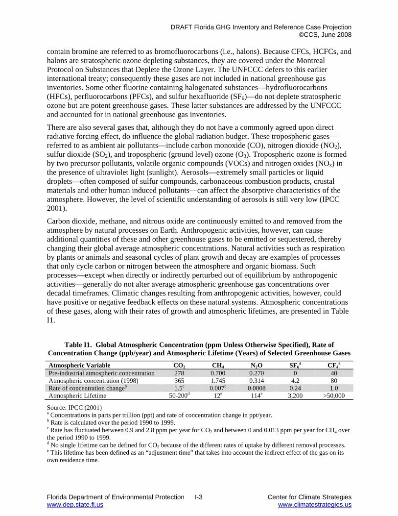
DRAFT Florida GHG Inventory and Reference Case Projection ©CCS, June 2008
Florida Department of Environmental Protection I-3 Center for Climate Strategies www.dep.state.fl.us www.climatestrategies.us
contain bromine are referred to as bromofluorocarbons (i.e., halons). Because CFCs, HCFCs, and halons are stratospheric ozone depleting substances, they are covered under the Montreal Protocol on Substances that Deplete the Ozone Layer. The UNFCCC defers to this earlier international treaty; consequently these gases are not included in national greenhouse gas inventories. Some other fluorine containing halogenated substances—hydrofluorocarbons (HFCs), perfluorocarbons (PFCs), and sulfur hexafluoride (SF6)—do not deplete stratospheric ozone but are potent greenhouse gases. These latter substances are addressed by the UNFCCC and accounted for in national greenhouse gas inventories.
There are also several gases that, although they do not have a commonly agreed upon direct radiative forcing effect, do influence the global radiation budget. These tropospheric gases—referred to as ambient air pollutants—include carbon monoxide (CO), nitrogen dioxide (NO2), sulfur dioxide (SO2), and tropospheric (ground level) ozone (O3). Tropospheric ozone is formed by two precursor pollutants, volatile organic compounds (VOCs) and nitrogen oxides (NOx) in the presence of ultraviolet light (sunlight). Aerosols—extremely small particles or liquid droplets—often composed of sulfur compounds, carbonaceous combustion products, crustal materials and other human induced pollutants—can affect the absorptive characteristics of the atmosphere. However, the level of scientific understanding of aerosols is still very low (IPCC 2001).
Carbon dioxide, methane, and nitrous oxide are continuously emitted to and removed from the atmosphere by natural processes on Earth. Anthropogenic activities, however, can cause additional quantities of these and other greenhouse gases to be emitted or sequestered, thereby changing their global average atmospheric concentrations. Natural activities such as respiration by plants or animals and seasonal cycles of plant growth and decay are examples of processes that only cycle carbon or nitrogen between the atmosphere and organic biomass. Such processes—except when directly or indirectly perturbed out of equilibrium by anthropogenic activities—generally do not alter average atmospheric greenhouse gas concentrations over decadal timeframes. Climatic changes resulting from anthropogenic activities, however, could have positive or negative feedback effects on these natural systems. Atmospheric concentrations of these gases, along with their rates of growth and atmospheric lifetimes, are presented in Table I1.
Table I1. Global Atmospheric Concentration (ppm Unless Otherwise Specified), Rate of Concentration Change (ppb/year) and Atmospheric Lifetime (Years) of Selected Greenhouse Gases
Atmospheric Variable CO2 CH4 N2O SF6a CF4
a Pre-industrial atmospheric concentration 278 0.700 0.270 0 40 Atmospheric concentration (1998) 365 1.745 0.314 4.2 80 Rate of concentration changeb 1.5c 0.007c 0.0008 0.24 1.0 Atmospheric Lifetime 50-200d 12e 114e 3,200 >50,000
Source: IPCC (2001) a Concentrations in parts per trillion (ppt) and rate of concentration change in ppt/year. b Rate is calculated over the period 1990 to 1999. c Rate has fluctuated between 0.9 and 2.8 ppm per year for CO2 and between 0 and 0.013 ppm per year for CH4 over the period 1990 to 1999. d No single lifetime can be defined for CO2 because of the different rates of uptake by different removal processes. e This lifetime has been defined as an “adjustment time” that takes into account the indirect effect of the gas on its own residence time.

DRAFT Florida GHG Inventory and Reference Case Projection ©CCS, June 2008
Florida Department of Environmental Protection I-4 Center for Climate Strategies www.dep.state.fl.us www.climatestrategies.us
A brief description of each greenhouse gas, its sources, and its role in the atmosphere is given below. The following section then explains the concept of Global Warming Potentials (GWPs), which are assigned to individual gases as a measure of their relative average global radiative forcing effect.
Water Vapor (H2O). Overall, the most abundant and dominant greenhouse gas in the atmosphere is water vapor. Water vapor is neither long-lived nor well mixed in the atmosphere, varying spatially from 0 to 2 percent (IPCC 1996). In addition, atmospheric water can exist in several physical states including gaseous, liquid, and solid. Human activities are not believed to directly affect the average global concentration of water vapor; however, the radiative forcing produced by the increased concentrations of other greenhouse gases may indirectly affect the hydrologic cycle. A warmer atmosphere has an increased water holding capacity; yet, increased concentrations of water vapor affects the formation of clouds, which can both absorb and reflect solar and terrestrial radiation. Aircraft contrails, which consist of water vapor and other aircraft emittants, are similar to clouds in their radiative forcing effects (IPCC 1999).
Carbon Dioxide (CO2). In nature, carbon is cycled between various atmospheric, oceanic, land biotic, marine biotic, and mineral reservoirs. The largest fluxes occur between the atmosphere and terrestrial biota, and between the atmosphere and surface water of the oceans. In the atmosphere, carbon predominantly exists in its oxidized form as CO2. Atmospheric carbon dioxide is part of this global carbon cycle, and therefore its fate is a complex function of geochemical and biological processes. Carbon dioxide concentrations in the atmosphere increased from approximately 280 parts per million by volume (ppmv) in pre-industrial times to 367 ppmv in 1999, a 31 percent increase (IPCC 2001). The IPCC notes that “[t]his concentration has not been exceeded during the past 420,000 years, and likely not during the past 20 million years. The rate of increase over the past century is unprecedented, at least during the past 20,000 years.” The IPCC definitively states that “the present atmospheric CO2 increase is caused by anthropogenic emissions of CO2” (IPCC 2001). Forest clearing, other biomass burning, and some non-energy production processes (e.g., cement production) also emit notable quantities of carbon dioxide.
In its second assessment, the IPCC also stated that “[t]he increased amount of carbon dioxide [in the atmosphere] is leading to climate change and will produce, on average, a global warming of the Earth’s surface because of its enhanced greenhouse effect—although the magnitude and significance of the effects are not fully resolved” (IPCC 1996).
Methane (CH4). Methane is primarily produced through anaerobic decomposition of organic matter in biological systems. Agricultural processes such as wetland rice cultivation, enteric fermentation in animals, and the decomposition of animal wastes emit CH4, as does the decomposition of municipal solid wastes. Methane is also emitted during the production and distribution of natural gas and petroleum, and is released as a by-product of coal mining and incomplete fossil fuel combustion. Atmospheric concentrations of methane have increased by about 150 percent since pre-industrial times, although the rate of increase has been declining. The IPCC has estimated that slightly more than half of the current CH4 flux to the atmosphere is anthropogenic, from human activities such as agriculture, fossil fuel use and waste disposal (IPCC 2001).
DRAFT Florida GHG Inventory and Reference Case Projection ©CCS, June 2008
Florida Department of Environmental Protection I-5 Center for Climate Strategies www.dep.state.fl.us www.climatestrategies.us
Methane is removed from the atmosphere by reacting with the hydroxyl radical (OH) and is ultimately converted to CO2. Minor removal processes also include reaction with Cl in the marine boundary layer, a soil sink, and stratospheric reactions. Increasing emissions of methane reduce the concentration of OH, a feedback which may increase methane’s atmospheric lifetime (IPCC 2001).
Nitrous Oxide (N2O). Anthropogenic sources of N2O emissions include agricultural soils, especially the use of synthetic and manure fertilizers; fossil fuel combustion, especially from mobile combustion; adipic (nylon) and nitric acid production; wastewater treatment and waste combustion; and biomass burning. The atmospheric concentration of nitrous oxide (N2O) has increased by 16 percent since 1750, from a pre industrial value of about 270 ppb to 314 ppb in 1998, a concentration that has not been exceeded during the last thousand years. Nitrous oxide is primarily removed from the atmosphere by the photolytic action of sunlight in the stratosphere.
Ozone (O3). Ozone is present in both the upper stratosphere, where it shields the Earth from harmful levels of ultraviolet radiation, and at lower concentrations in the troposphere, where it is the main component of anthropogenic photochemical “smog.” During the last two decades, emissions of anthropogenic chlorine and bromine-containing halocarbons, such as chlorofluorocarbons (CFCs), have depleted stratospheric ozone concentrations. This loss of ozone in the stratosphere has resulted in negative radiative forcing, representing an indirect effect of anthropogenic emissions of chlorine and bromine compounds (IPCC 1996). The depletion of stratospheric ozone and its radiative forcing was expected to reach a maximum in about 2000 before starting to recover, with detection of such recovery not expected to occur much before 2010 (IPCC 2001).
The past increase in tropospheric ozone, which is also a greenhouse gas, is estimated to provide the third largest increase in direct radiative forcing since the pre-industrial era, behind CO2 and CH4. Tropospheric ozone is produced from complex chemical reactions of volatile organic compounds mixing with nitrogen oxides (NOx) in the presence of sunlight. Ozone, carbon monoxide (CO), sulfur dioxide (SO2), nitrogen dioxide (NO2) and particulate matter are included in the category referred to as “criteria pollutants” in the United States under the Clean Air Act and its subsequent amendments. The tropospheric concentrations of ozone and these other pollutants are short-lived and, therefore, spatially variable.
Halocarbons, Perfluorocarbons, and Sulfur Hexafluoride (SF6). Halocarbons are, for the most part, man-made chemicals that have both direct and indirect radiative forcing effects. Halocarbons that contain chlorine—chlorofluorocarbons (CFCs), hydrochlorofluorocarbons (HCFCs), methyl chloroform, and carbon tetrachloride—and bromine—halons, methyl bromide, and hydrobromofluorocarbons (HBFCs)—result in stratospheric ozone depletion and are therefore controlled under the Montreal Protocol on Substances that Deplete the Ozone Layer. Although CFCs and HCFCs include potent global warming gases, their net radiative forcing effect on the atmosphere is reduced because they cause stratospheric ozone depletion, which is itself an important greenhouse gas in addition to shielding the Earth from harmful levels of ultraviolet radiation. Under the Montreal Protocol, the United States phased out the production and importation of halons by 1994 and of CFCs by 1996. Under the Copenhagen Amendments to the Protocol, a cap was placed on the production and importation of HCFCs by non-Article 5 countries beginning in 1996, and then followed by a complete phase-out by the year 2030. The ozone depleting gases covered under the Montreal Protocol and its Amendments are not covered by the UNFCCC.
DRAFT Florida GHG Inventory and Reference Case Projection ©CCS, June 2008
Florida Department of Environmental Protection I-6 Center for Climate Strategies www.dep.state.fl.us www.climatestrategies.us
Hydrofluorocarbons (HFCs), perfluorocarbons (PFCs), and sulfur hexafluoride (SF6) are not ozone depleting substances, and therefore are not covered under the Montreal Protocol. They are, however, powerful greenhouse gases. HFCs—primarily used as replacements for ozone depleting substances but also emitted as a by-product of the HCFC-22 manufacturing process—currently have a small aggregate radiative forcing impact; however, it is anticipated that their contribution to overall radiative forcing will increase (IPCC 2001). PFCs and SF6 are predominantly emitted from various industrial processes including aluminum smelting, semiconductor manufacturing, electric power transmission and distribution, and magnesium casting. Currently, the radiative forcing impact of PFCs and SF6 is also small; however, they have a significant growth rate, extremely long atmospheric lifetimes, and are strong absorbers of infrared radiation, and therefore have the potential to influence climate far into the future (IPCC 2001).
Carbon Monoxide (CO). Carbon monoxide has an indirect radiative forcing effect by elevating concentrations of CH4 and tropospheric ozone through chemical reactions with other atmospheric constituents (e.g., the hydroxyl radical, OH) that would otherwise assist in destroying CH4 and tropospheric ozone. Carbon monoxide is created when carbon-containing fuels are burned incompletely. Through natural processes in the atmosphere, it is eventually oxidized to CO2. Carbon monoxide concentrations are both short-lived in the atmosphere and spatially variable.
Nitrogen Oxides (NOx). The primary climate change effects of nitrogen oxides (i.e., NO and NO2) are indirect and result from their role in promoting the formation of ozone in the troposphere and, to a lesser degree, lower stratosphere, where it has positive radiative forcing effects. Additionally, NOx emissions from aircraft are also likely to decrease methane concentrations, thus having a negative radiative forcing effect (IPCC 1999). Nitrogen oxides are created from lightning, soil microbial activity, biomass burning – both natural and anthropogenic fires – fuel combustion, and, in the stratosphere, from the photo-degradation of nitrous oxide (N2O). Concentrations of NOx are both relatively short-lived in the atmosphere and spatially variable.
Nonmethane Volatile Organic Compounds (NMVOCs). Nonmethane volatile organic compounds include compounds such as propane, butane, and ethane. These compounds participate, along with NOx, in the formation of tropospheric ozone and other photochemical oxidants. NMVOCs are emitted primarily from transportation and industrial processes, as well as biomass burning and non-industrial consumption of organic solvents. Concentrations of NMVOCs tend to be both short-lived in the atmosphere and spatially variable.
Aerosols. Aerosols are extremely small particles or liquid droplets found in the atmosphere. They can be produced by natural events such as dust storms and volcanic activity, or by anthropogenic processes such as fuel combustion and biomass burning. They affect radiative forcing in both direct and indirect ways: directly by scattering and absorbing solar and thermal infrared radiation; and indirectly by increasing droplet counts that modify the formation, precipitation efficiency, and radiative properties of clouds. Aerosols are removed from the atmosphere relatively rapidly by precipitation. Because aerosols generally have short atmospheric lifetimes, and have concentrations and compositions that vary regionally, spatially, and temporally, their contributions to radiative forcing are difficult to quantify (IPCC 2001).

DRAFT Florida GHG Inventory and Reference Case Projection ©CCS, June 2008
Florida Department of Environmental Protection I-7 Center for Climate Strategies www.dep.state.fl.us www.climatestrategies.us
The indirect radiative forcing from aerosols is typically divided into two effects. The first effect involves decreased droplet size and increased droplet concentration resulting from an increase in airborne aerosols. The second effect involves an increase in the water content and lifetime of clouds due to the effect of reduced droplet size on precipitation efficiency (IPCC 2001). Recent research has placed a greater focus on the second indirect radiative forcing effect of aerosols.
Various categories of aerosols exist, including naturally produced aerosols such as soil dust, sea salt, biogenic aerosols, sulphates, and volcanic aerosols, and anthropogenically manufactured aerosols such as industrial dust and carbonaceous aerosols (e.g., black carbon, organic carbon) from transportation, coal combustion, cement manufacturing, waste incineration, and biomass burning.
The net effect of aerosols is believed to produce a negative radiative forcing effect (i.e., net cooling effect on the climate), although because they are short-lived in the atmosphere—lasting days to weeks—their concentrations respond rapidly to changes in emissions. Locally, the negative radiative forcing effects of aerosols can offset the positive forcing of greenhouse gases (IPCC 1996). “However, the aerosol effects do not cancel the global-scale effects of the much longer-lived greenhouse gases, and significant climate changes can still result” (IPCC 1996).
The IPCC’s Third Assessment Report notes that “the indirect radiative effect of aerosols is now understood to also encompass effects on ice and mixed-phase clouds, but the magnitude of any such indirect effect is not known, although it is likely to be positive” (IPCC 2001). Additionally, current research suggests that another constituent of aerosols, elemental carbon, may have a positive radiative forcing (Jacobson 2001). The primary anthropogenic emission sources of elemental carbon include diesel exhaust, coal combustion, and biomass burning.
Global Warming Potentials Global Warming Potentials (GWPs) are intended as a quantified measure of the globally averaged relative radiative forcing impacts of a particular greenhouse gas. It is defined as the cumulative radiative forcing⎯both direct and indirect effects⎯integrated over a period of time from the emission of a unit mass of gas relative to some reference gas (IPCC 1996). Carbon dioxide (CO2) was chosen as this reference gas. Direct effects occur when the gas itself is a greenhouse gas. Indirect radiative forcing occurs when chemical transformations involving the original gas produce a gas or gases that are greenhouse gases, or when a gas influences other radiatively important processes such as the atmospheric lifetimes of other gases. The relationship between gigagrams (Gg) of a gas and Tg CO2 Eq. can be expressed as follows:
( ) ( ) ⎟⎟⎠
⎞⎜⎜⎝
⎛××=
Gg 1,000TgGWPgasofGgEq CO Tg 2 where,
Tg CO2 Eq. = Teragrams of Carbon Dioxide Equivalents Gg = Gigagrams (equivalent to a thousand metric tons)
GWP = Global Warming Potential Tg = Teragrams
GWP values allow policy makers to compare the impacts of emissions and reductions of different gases. According to the IPCC, GWPs typically have an uncertainty of roughly ±35 percent, though some GWPs have larger uncertainty than others, especially those in which lifetimes have not yet been ascertained. In the following decision, the parties to the UNFCCC have agreed to use consistent GWPs from the IPCC Second Assessment Report (SAR), based upon a 100 year time horizon, although other time horizon values are available (see Table I2).
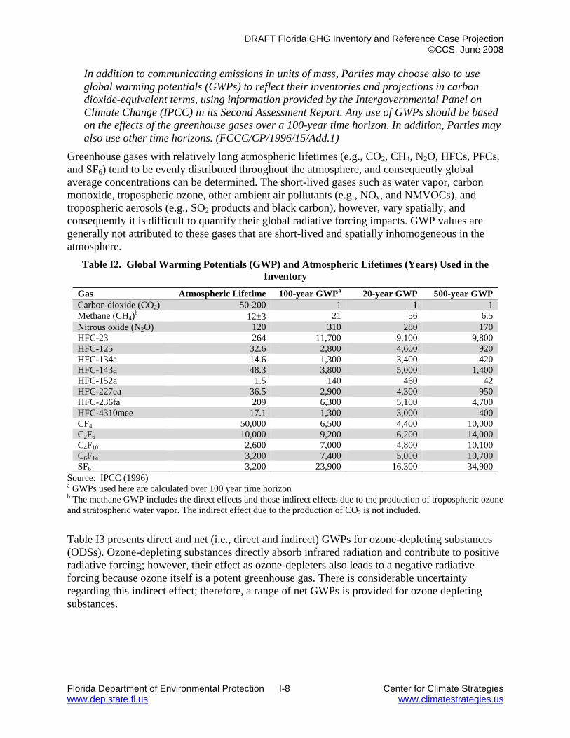
DRAFT Florida GHG Inventory and Reference Case Projection ©CCS, June 2008
Florida Department of Environmental Protection I-8 Center for Climate Strategies www.dep.state.fl.us www.climatestrategies.us
In addition to communicating emissions in units of mass, Parties may choose also to use global warming potentials (GWPs) to reflect their inventories and projections in carbon dioxide-equivalent terms, using information provided by the Intergovernmental Panel on Climate Change (IPCC) in its Second Assessment Report. Any use of GWPs should be based on the effects of the greenhouse gases over a 100-year time horizon. In addition, Parties may also use other time horizons. (FCCC/CP/1996/15/Add.1)
Greenhouse gases with relatively long atmospheric lifetimes (e.g., CO2, CH4, N2O, HFCs, PFCs, and SF6) tend to be evenly distributed throughout the atmosphere, and consequently global average concentrations can be determined. The short-lived gases such as water vapor, carbon monoxide, tropospheric ozone, other ambient air pollutants (e.g., NOx, and NMVOCs), and tropospheric aerosols (e.g., SO2 products and black carbon), however, vary spatially, and consequently it is difficult to quantify their global radiative forcing impacts. GWP values are generally not attributed to these gases that are short-lived and spatially inhomogeneous in the atmosphere.
Table I2. Global Warming Potentials (GWP) and Atmospheric Lifetimes (Years) Used in the Inventory
Gas Atmospheric Lifetime 100-year GWPa 20-year GWP 500-year GWP Carbon dioxide (CO2) 50-200 1 1 1 Methane (CH4)b 12±3 21 56 6.5 Nitrous oxide (N2O) 120 310 280 170 HFC-23 264 11,700 9,100 9,800 HFC-125 32.6 2,800 4,600 920 HFC-134a 14.6 1,300 3,400 420 HFC-143a 48.3 3,800 5,000 1,400 HFC-152a 1.5 140 460 42 HFC-227ea 36.5 2,900 4,300 950 HFC-236fa 209 6,300 5,100 4,700 HFC-4310mee 17.1 1,300 3,000 400 CF4 50,000 6,500 4,400 10,000 C2F6 10,000 9,200 6,200 14,000 C4F10 2,600 7,000 4,800 10,100 C6F14 3,200 7,400 5,000 10,700 SF6 3,200 23,900 16,300 34,900
Source: IPCC (1996) a GWPs used here are calculated over 100 year time horizon b The methane GWP includes the direct effects and those indirect effects due to the production of tropospheric ozone and stratospheric water vapor. The indirect effect due to the production of CO2 is not included.
Table I3 presents direct and net (i.e., direct and indirect) GWPs for ozone-depleting substances (ODSs). Ozone-depleting substances directly absorb infrared radiation and contribute to positive radiative forcing; however, their effect as ozone-depleters also leads to a negative radiative forcing because ozone itself is a potent greenhouse gas. There is considerable uncertainty regarding this indirect effect; therefore, a range of net GWPs is provided for ozone depleting substances.
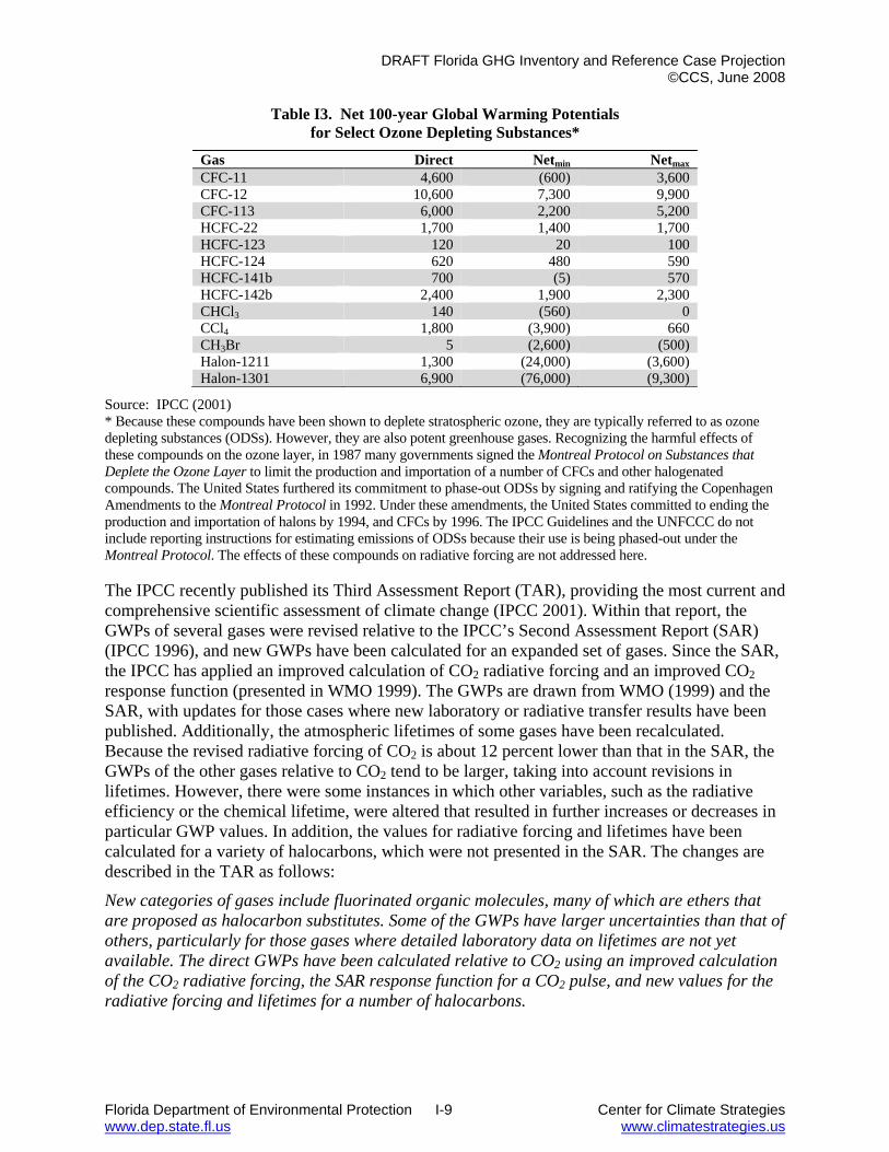
DRAFT Florida GHG Inventory and Reference Case Projection ©CCS, June 2008
Florida Department of Environmental Protection I-9 Center for Climate Strategies www.dep.state.fl.us www.climatestrategies.us
Table I3. Net 100-year Global Warming Potentials for Select Ozone Depleting Substances*
Gas Direct Netmin Netmax CFC-11 4,600 (600) 3,600 CFC-12 10,600 7,300 9,900 CFC-113 6,000 2,200 5,200 HCFC-22 1,700 1,400 1,700 HCFC-123 120 20 100 HCFC-124 620 480 590 HCFC-141b 700 (5) 570 HCFC-142b 2,400 1,900 2,300 CHCl3 140 (560) 0 CCl4 1,800 (3,900) 660 CH3Br 5 (2,600) (500) Halon-1211 1,300 (24,000) (3,600) Halon-1301 6,900 (76,000) (9,300)
Source: IPCC (2001) * Because these compounds have been shown to deplete stratospheric ozone, they are typically referred to as ozone depleting substances (ODSs). However, they are also potent greenhouse gases. Recognizing the harmful effects of these compounds on the ozone layer, in 1987 many governments signed the Montreal Protocol on Substances that Deplete the Ozone Layer to limit the production and importation of a number of CFCs and other halogenated compounds. The United States furthered its commitment to phase-out ODSs by signing and ratifying the Copenhagen Amendments to the Montreal Protocol in 1992. Under these amendments, the United States committed to ending the production and importation of halons by 1994, and CFCs by 1996. The IPCC Guidelines and the UNFCCC do not include reporting instructions for estimating emissions of ODSs because their use is being phased-out under the Montreal Protocol. The effects of these compounds on radiative forcing are not addressed here. The IPCC recently published its Third Assessment Report (TAR), providing the most current and comprehensive scientific assessment of climate change (IPCC 2001). Within that report, the GWPs of several gases were revised relative to the IPCC’s Second Assessment Report (SAR) (IPCC 1996), and new GWPs have been calculated for an expanded set of gases. Since the SAR, the IPCC has applied an improved calculation of CO2 radiative forcing and an improved CO2 response function (presented in WMO 1999). The GWPs are drawn from WMO (1999) and the SAR, with updates for those cases where new laboratory or radiative transfer results have been published. Additionally, the atmospheric lifetimes of some gases have been recalculated. Because the revised radiative forcing of CO2 is about 12 percent lower than that in the SAR, the GWPs of the other gases relative to CO2 tend to be larger, taking into account revisions in lifetimes. However, there were some instances in which other variables, such as the radiative efficiency or the chemical lifetime, were altered that resulted in further increases or decreases in particular GWP values. In addition, the values for radiative forcing and lifetimes have been calculated for a variety of halocarbons, which were not presented in the SAR. The changes are described in the TAR as follows:
New categories of gases include fluorinated organic molecules, many of which are ethers that are proposed as halocarbon substitutes. Some of the GWPs have larger uncertainties than that of others, particularly for those gases where detailed laboratory data on lifetimes are not yet available. The direct GWPs have been calculated relative to CO2 using an improved calculation of the CO2 radiative forcing, the SAR response function for a CO2 pulse, and new values for the radiative forcing and lifetimes for a number of halocarbons.

DRAFT Florida GHG Inventory and Reference Case Projection ©CCS, June 2008
Florida Department of Environmental Protection I-10 Center for Climate Strategies www.dep.state.fl.us www.climatestrategies.us
References FCCC (1996) Framework Convention on Climate Change; FCCC/CP/1996/15/Add.1; 29 October 1996; Report of the Conference of the Parties at its second session. Revised Guidelines for the Preparation of National Communications by Parties Included in Annex I to the Convention, p18. Geneva 1996.
IPCC (2001) Climate Change 2001: A Scientific Basis, Intergovernmental Panel on Climate Change; J.T. Houghton, Y. Ding, D.J. Griggs, M. Noguer, P.J. van der Linden, X. Dai, C.A. Johnson, and K. Maskell, eds.; Cambridge University Press. Cambridge, U.K.
IPCC (2000) Good Practice Guidance and Uncertainty Management in National Greenhouse Gas Inventories. IPCC National Greenhouse Gas Inventories Programme Technical Support Unit, Kanagawa, Japan. Available online at <http://www.ipcc-nggip.iges.or.jp/gp/report.htm>.
IPCC (1999) Aviation and the Global Atmosphere. Intergovernmental Panel on Climate Change; Penner, J.E., et al., eds.; Cambridge University Press. Cambridge, U.K.
IPCC (1996) Climate Change 1995: The Science of Climate Change. Intergovernmental Panel on Climate Change; J.T. Houghton, L.G. Meira Filho, B.A. Callander, N. Harris, A. Kattenberg, and K. Maskell, eds.; Cambridge University Press. Cambridge, U.K.
IPCC/UNEP/OECD/IEA (1997) Revised 1996 IPCC Guidelines for National Greenhouse Gas Inventories. Paris: Intergovernmental Panel on Climate Change, United Nations Environment Programme, Organization for Economic Co-Operation and Development, International Energy Agency.
Jacobson, M.Z. (2001) Strong Radiative Heating Due to the Mixing State ofBlack Carbon in Atmospheric Aerosols. Nature. In press.
UNEP/WMO (2000) Information Unit on Climate Change. Framework Convention on Climate Change (Available on the internet at <http://www.unfccc.de>.)
WMO (1999) Scientific Assessment of Ozone Depletion, Global Ozone Research and Monitoring Project-Report No. 44, World Meteorological Organization, Geneva, Switzerland.