EE263 Prof. S. BoydDec. 8–9 or Dec. 9–10, 2006.

Final exam solutions

1. Analysis and optimization of a communication network. A communication networkis modeled as a set of m directed links connecting nodes. There are n routes in thenetwork. A route is a path, along one or more links in the network, from a source nodeto a destination node. In this problem, the routes are fixed, and are described by anm× n route-link matrix A, defined as

Aij =

{

1 route j passes through link i0 otherwise.

Over each route we have a nonnegative flow, measured in (say) bits per second. Wedenote the flow along route j as fj, and we call f ∈ Rn the flow vector. The traffic ona link i, denoted ti, is the sum of the flows on all routes passing through link i. Thevector t ∈ Rm is called the traffic vector.

Each link has an associated nonnegative delay, measured in (say) seconds. We denotethe delay for link i as di, and refer to d ∈ Rm as the link delay vector. The latency ona route j, denoted lj, is the sum of the delays along each link constituting the route,i.e., the time it takes for bits entering the source to emerge at the destination. Thevector l ∈ Rn is the route latency vector.

The total number of bits in the network at an instant in time is given by B = fT l = tTd.

(a) Worst-case flows and delays. Suppose the flows and link delays satisfy

(1/n)n

∑

j=1

f 2j ≤ F 2, (1/m)

m∑

i=1

d2i ≤ D2,

where F and D are given. What is the maximum possible number of bits in thenetwork? What values of f and d achieve this maximum value? (For this problemyou can ignore the constraint that the flows and delays must be nonnegative. Itturns out, however, that the worst-case flows and delays can always be chosen tobe nonnegative.)

(b) Utility maximization. For a flow fj, the network operator derives income at a ratepjfj, where pj is the price per unit flow on route j. The network operator’s totalrate of income is thus

∑nj=1 pjfj. (The route prices are known and positive.)

The network operator is charged at a rate citi for having traffic ti on link i, whereci is the cost per unit of traffic on link i. The total charge rate for link traffic

1

is∑m

i=1 tici. (The link costs are known and positive.) The net income rate (orutility) to the network operator is therefore

Unet =n

∑

j=1

pjfj −m

∑

i=1

citi.

Find the flow vector f that maximizes the operator’s net income rate, subject tothe constraint that each fj is between 0 and Fmax, where Fmax is a given positivemaximum flow value.

Solution: The traffic vector t is given by t = Af , and the route latency vector l isgiven by l = ATd.

(a) The number of bits in the network is given by B = dTAf . The problem, then, isto find

Bmax = max‖f‖2≤nF 2, ‖d‖2≤mD2

dTAf.

We know that, for any f and d satisfying the constraints, we have

dTAf ≤ ‖d‖‖A‖‖f‖ ≤ FD√mn‖A‖.

It follows that Bmax ≤ FD√mn‖A‖. We are now going to show that equality

holds here.

Consider the choices

f = F√nvmax, d = D

√mumax,

where vmax and umax are, respectively, the right and left singular vectors with unitnorm, associated with ‖A‖, the largest singular value of A. For these choices wehave

dTAf = FD√mnuT

maxAvmax = FD√mnuT

max‖A‖umax = FD√mn‖A‖.

The maximum number of bits in the network is therefore

Bmax = FD√mn‖A‖.

(b) Let p ∈ Rn be the vector whose jth entry is pj and let c ∈ Rm be the vectorwhose ith entry is ci. The net income rate of the network is given by

Unet = pTf − cT t = pTf − cTAf = (p− AT c)Tf.

We need to find the flow distribution f that solves the following problem:

maximize (p− AT c)Tfsubject to 0 ≤ f ≤ Fmax.

2

Now it looks like the Cauchy-Schwarz inequality should be useful here, since we arechoosing a vector (f) to maximize its inner product with another vector (p−AT c).However, the constraint on f is not on its norm, so Cauchy-Schwarz isn’t relevanthere.

Defining w = p − AT c, the objective is to maximize∑

iwifi subject to 0 ≤ fi ≤Fmax. We can choose the fi’s separately (since the constraints involve each fi

separately, and the objective is a sum of terms, each involving only fi). If wi isnegative, it means that the costs for route i exceed income, so the best we can dois set fi = 0. If wi > 0, which means that the revenue exceeds the cost, we shouldset fi = Fmax.

In summary, the solution is given by

fj =

{

Fmax wj > 00 wj ≤ 0

for j = 1, . . . , p.

We can give a very simple interpretation of this optimal flow. The number wj isexactly the revenue per unit flow j (i.e., pj) minus the total link cost per unitflow over all the links that route j goes over (i.e., (AT c)j). If this net number ispositive, then we set the flow to its maximum value (in order to get the maximumnet utility). If this net number is negative, we set the flow to zero.

3

2. Stability of a time-varying system. We consider a discrete-time linear dynamical system

x(t+ 1) = A(t)x(t),

where A(t) ∈ {A1, A2, A3, A4}. These 4 matrices, which are 4 × 4, are given intv_data.m.

Show that this system is stable, i.e., for any trajectory x, we have x(t) → 0 as t→ ∞.(This means that for any x(0), and for any sequence A(0), A(1), A(2), . . ., we havex(t) → 0 as t→ ∞.)

You may use any methods or concepts used in the class, e.g., least-squares, eigenvalues,singular values, controllability, and so on. Your proof will consist of two parts:

• An explanation of how you are going to show that any trajectory converges tozero. Your argument of course will require certain conditions (that you will find)to hold for the given data A1, . . . , A4.

• The numerical calculations that verify the conditions hold for the given data. Youmust provide the source code for these calculations, and show the results as well.

Your answer is limited to three pages, including the numerical verification.

We will not read past three pages. Of course, you are welcome to submit a solutionthat is shorter than three pages!

Solution.First some discussion. We can check that each of the matrices Ai is stable, i.e., alleigenvalues have magnitude less than one. Of course this has to be the case, becausea possible sequence is A(t) = Ai for all t. But this certainly does not prove that thetime-varying system is stable. Simple examples show that time-varying systems canbe unstable, even when for each t, A(t) is stable.

As far as we know, no argument based on the magnitude of eigenvalues (of any matrixor matrices) is correct. Basically, eigenvalues were just not relevant in this problem.

Instead, we are going to argue that the norm of the state decreases to zero. We findthat the maximum gains (matrix norms) of the matrices are:

norm(A1) = 6.016509

norm(A2) = 5.007023

norm(A3) = 1.999188

norm(A4) = 0.149993

This shows that multiplication by A4 does indeed reduce the norm of a vector, by afactor less than one. But the matrices A1, A2, and A3 can amplify the norm of a vectorby factors much larger than one. In particular, it’s not true that the norm of x(t)decreases at each step. But we note, for future use, that ‖x(t+ 1)‖ ≤ 6.02‖x(t)‖.Now we examine the gain of products of pairs of the matrices.

4

norm(A1*A1) = 0.163270

norm(A1*A2) = 0.498489

norm(A1*A3) = 0.907308

norm(A1*A4) = 0.836615

norm(A2*A1) = 0.149617

norm(A2*A2) = 0.253311

norm(A2*A3) = 0.754820

norm(A2*A4) = 0.696261

norm(A3*A1) = 0.484295

norm(A3*A2) = 0.753466

norm(A3*A3) = 0.795547

norm(A3*A4) = 0.278107

norm(A4*A1) = 0.832049

norm(A4*A2) = 0.474458

norm(A4*A3) = 0.228314

norm(A4*A4) = 0.018116

There are sixteen such pairs, and it turns out the maximum gain (matrix norm) of allsuch pairs is less than one. In fact, they are all less than 0.91. This means that forany x(t), and any values of A(t) and A(t+ 1), we have

‖x(t+ 2)‖ = ‖A(t+ 1)A(t)x(t)‖ ≤ ‖A(t+ 1)A(t)‖‖x(t)‖ ≤ 0.91‖x(t)‖.

Thus, in any two steps, the norm of x(t) does indeed decrease! This implies that

‖x(2k)‖ ≤ 0.91k‖x(0)‖.

We also have‖x(2k + 1)‖ ≤ 6.02‖x(2k)‖ ≤ (6.02)0.91k‖x(0)‖.

Therefore we have ‖x(t)‖ → 0 as t→ ∞, which means x(t) → 0 as t→ ∞.

We mention one other valid approach that a few people used. We have already seenthat the norms of 3 of the 4 matrices exceed one, which means that in any given step,the norm of the state can increase. This approach is based on changing coordinates sothat, in the new coordinates, the norm of the state decreases at every step.

Suppose we can find a nonsingular matrix T for which ‖T−1AiT‖ < 1 for i = 1, . . . , 4.Then the original system is stable, i.e., all trajectories converge to zero. To see this,we note that

‖T−1x(t)‖ = ‖T−1A(t− 1) · · ·A(0)x(0)‖= ‖T−1A(t− 1)T · · ·T−1A(0)TT−1x(0)‖≤ αt‖T−1x(0)‖,

where α = maxi ‖T−1AiT‖ < 1. What this shows is that at every step, ‖T−1x‖decreases.

5

Now, how do you find such a T? This has a really good answer, which is well beyondEE263 (it’s a convex problem, and can be solved using semidefinite programmingand linear matrix inequalities). A few people found a valid T using random or othersearches. As long as the method was clearly described, we can gave full credit for thisapproach.

We mention a few methods that are wrong. As mentioned above, any method thatrelies on eigenvalues, of any martix or matrices, is wrong.

One hand-waving method observed that the maximum gain output directions of eachmatrix didn’t line up with the maximum gain input directions of any other matrix.(We saw several variations on this basic theme.) Well, that may be true, but we don’tsee what it proves.

Others tried to ‘prove’ that x(t) goes to zero by simulating. Of course, that’s not aproof. By the way, we wouldn’t ask you to prove something that’s false (at least notintentionally), so the fact that x(t) converges to zero wasn’t in question. We asked youto prove it.

6

3. Some bounds on singular values. Suppose A ∈ R6×3, with singular values 7, 5, 3,and B ∈ R6×3, with singular values 2, 2, 1. Let C = [A B] ∈ R6×6, with full SVDC = UΣV T , with Σ = diag(σ1, . . . , σ6). (We allow the possibility that some of thesesingular values are zero.)

(a) How large can σ1 be?

(b) How small can σ1 be?

(c) How large can σ6 be?

(d) How small can σ6 be?

What we mean is, how large (or small) can the specified quantity be, for any A and Bwith the given sizes and given singular values.

Please give only the answers, as specific numbers, with 3 digits after the

decimal place. We’re looking for answers that have the form

(a) 12.420, (b) 10.000, (c) 0.552, (d) 0.000

(This is just an example). We will not read any derivation or justification. You do nothave to find A and B that achieve the values you give.

Solution: The solution is

(a)√

72 + 22 = 7.28, (b) 7, (c) 1, (d) 0.

We didn’t ask you to justify your answers, but of course we will. We start by writing

∥

∥

∥

∥

∥

[A B]

[

uv

]∥

∥

∥

∥

∥

= ‖Au+Bv‖,

where u, v ∈ R3.

(a) First we note that

∥

∥

∥

∥

∥

[A B]

[

uv

]∥

∥

∥

∥

∥

= ‖Au+Bv‖ ≤ ‖Au‖ + ‖Bv‖ ≤ 7‖u‖ + 2‖v‖.

Now we ask: how large can 7‖u‖ + 2‖v‖ be, over all u and v with

∥

∥

∥

∥

∥

[

uv

]∥

∥

∥

∥

∥

=√

‖u‖2 + ‖v‖2 ≤ 1.

This is just Cauchy-Schwarz: it can be no larger than√

72 + 22. Thus, for anymatrices A and B with the given singular values, we have ‖C‖ ≤

√72 + 22. Could

7

‖C‖ actually be this large? Yes: take

A =

7 0 00 5 00 0 30 0 00 0 00 0 0

, B =

2 0 00 2 00 0 10 0 00 0 00 0 0

, u =1√

72 + 22

700200

.

We have ‖C[uT vT ]T‖ =√

72 + 22.

(b) Taking u to be the right singular vector of A associated with its largest singularvalue (i.e., 7), and v zero, we find that

∥

∥

∥

∥

∥

[

u0

]∥

∥

∥

∥

∥

= 1,

∥

∥

∥

∥

∥

[A B]

[

u0

]∥

∥

∥

∥

∥

= ‖Au‖ = 7.

This shows that the norm of C must be at least 7. Can it be 7? The answer isyes: just take

A =

7 0 00 5 00 0 30 0 00 0 00 0 0

, B =

0 0 00 0 00 0 02 0 00 2 00 0 1

.

These matrices have the required singular values, and C is diagonal, evidentlywith ‖C‖ = 7. So the answer to part (b) is 7.

(c) Taking u zero and v to be the right singular vector of B associated with itssmallest singular value (i.e., 1), we have ‖C[uT vT ]T‖ = 1. The minimum gain ofC could only be smaller, so we conclude that for any A and B we have σ6 ≤ 1.Could we attain this value for some choice of A and B? Yes:

A =

7 0 00 5 00 0 30 0 00 0 00 0 0

, B =

0 0 00 0 00 0 02 0 00 2 00 0 1

.

For these A and B, C is diagonal and has σ6 = 1.

(d) The answer 0 is justified by

A =

7 0 00 5 00 0 30 0 00 0 00 0 0

, B =

2 0 00 2 00 0 10 0 00 0 00 0 0

,

8

for which σ6 = 0.

9

4. Optimal choice of initial temperature profile. We consider a thermal system describedby an n-element finite-element model. The elements are arranged in a line, with thetemperature of element i at time t denoted Ti(t). Temperature is measured in degreesCelsius above ambient; negative Ti(t) corresponds to a temperature below ambient.The dynamics of the system are described by

c1T1 = −a1T1 − b1(T1 − T2),

ciTi = −aiTi − bi(Ti − Ti+1) − bi−1(Ti − Ti−1), i = 2, . . . , n− 1,

andcnTn = −anTn − bn−1(Tn − Tn−1).

where c ∈ Rn, a ∈ Rn, and b ∈ Rn−1 are given and are all positive.

We can interpret this model as follows. The parameter ci is the heat capacity ofelement i, so ciTi is the net heat flow into element i. The parameter ai gives thethermal conductance between element i and the environment, so aiTi is the heat flowfrom element i to the environment (i.e., the direct heat loss from element i.) Theparameter bi gives the thermal conductance between element i and element i + 1, sobi(Ti − Ti+1) is the heat flow from element i to element i + 1. Finally, bi−1(Ti − Ti−1)is the heat flow from element i to element i− 1.

The goal of this problem is to choose the initial temperature profile, T (0) ∈ Rn, sothat T (tdes) ≈ T des. Here, tdes ∈ R is a specific time when we want the temperatureprofile to closely match T des ∈ Rn. We also wish to satisfy a constraint that ‖T (0)‖should be not be too large.

To formalize these requirements, we use the objective (1/√n)‖T (tdes) − T des‖ and

the constraint (1/√n)‖T (0)‖ ≤ Tmax. The first expression is the RMS temperature

deviation, at t = tdes, from the desired value, and the second is the RMS temperaturedeviation from ambient at t = 0. Tmax is the (given) maximum inital RMS temperaturevalue.

(a) Explain how to find T (0) that minimizes the objective while satisfying the con-straint.

(b) Solve the problem instance with the values of n, c, a, b, tdes, Tdes and Tmax defined

in the file temp_prof_data.m.

Plot, on one graph, your T (0), T (tdes) and T des. Give the RMS temperature error(1/

√n)‖T (tdes)−T des‖, and the RMS value of initial temperature (1/

√n)‖T (0)‖.

Solution.

(a) We can express the temperature dynamics as T = AT , where A is a tridiagonalmatrix with

A11 = −1/c1(a1 + b1)

10

Aii = −1/ci(ai + bi + bi−1), i = 2, . . . , n,

Ai,i−1 = bi−1/ci, i = 2, . . . , n,

Ai,i+1 = bi/ci, i = 1, . . . , n− 1.

We have T (tdes) = etdesAT (0). Therefore we must solve the problem

minimize (1/n)∥

∥

∥etdesAT (0) − T des∥

∥

∥

2

subject to (1/n)‖T (0)‖2 ≤ (Tmax)2.

We solve this by minimizing

∥

∥

∥etdesAT (0) − T des∥

∥

∥

2

+ ρ‖T (0)‖2,

and increasing ρ until (1/n)‖T (0)‖2 ≤ (Tmax)2 first holds (which will be withequality).

We mention one rather common error: simply obtaining the least-squares solution(without regards for ‖T (0)‖, and then scaling this solution down so that theconstraint is satisfied. This method produces results that look pretty good, whenplotted, but are in fact not particularly good (in addition to just being wrong).This results in an RMS temperature error that more than 60% higher than usingthe correct method.

(b) The following code solves the problem in part (b).

clear all; close all

temp_prof_data

A(1,1)=-1/c(1)*(a(1)+b(1));

A(1,2)=b(1)/c(1);

A(n,n)=-1/c(n)*(a(n)+b(n-1));

A(n,n-1)=b(n-1)/c(n);

for i=2:n-1

A(i,i)=-1/c(i)*(a(i)+b(i)+b(i-1));

A(i,i-1)=b(i-1)/c(i);

A(i,i+1)=b(i)/c(i);

end

B=expm(A*tdes);

rho=0;

while 1

C=[B; sqrt(rho)*eye(n)];

d=[Tdes;zeros(n,1)];

11

0 20 40 60 80 100−6

−4

−2

0

2

4

6

8

T

i

Figure 1: Tdes (solid blue), T (tdes) (dashed red) and T (0) (dash-dotted black).

T=C\d;

if norm(T)/sqrt(n)<=Tmax

break

end

rho=rho+1e-5;

end

plot(Tdes); hold on

plot(B*T,’xr’);

plot(T,’k’); hold off

set(gca,’Fontname’,’Times’,’Fontsize’, 16);

ylabel(’t’); xlabel(’x’)

print -depsc temp_prof

norm(T)/sqrt(n)

norm(Tdes-B*T)/sqrt(n)

Figure 1 shows T des with a solid blue line, T (tdes) with a dashed red line and T (0)with a dash-dotted black line. We have (1/

√n)‖T (tdes)− T des‖ = 0.0457, and, as

expected, (1/√n)‖T (0)‖ = 2.50.

12

5. A heuristic for MAXCUT. Consider a graph with n nodes and m edges, with thenodes labeled 1, . . . , n and the edges labeled 1, . . . ,m. We partition the nodes into twogroups, B and C, i.e., B ∩ C = ∅, B ∪ C = {1, . . . , n}. We define the number of cutsassociated with this partition as the number of edges between pairs of nodes when oneof the nodes is in B and the other is in C. A famous problem, called the MAXCUTproblem, involves choosing a partition (i.e., B and C) that maximizes the number ofcuts for a given graph. For any partition, the number of cuts can be no more than m.If the number of cuts is m, nodes in group B connect only to nodes in group C andthe graph is bipartite.

The MAXCUT problem has many applications. We describe one here, although youdo not need it to solve this problem. Suppose we have a communication system thatoperates with a two-phase clock. During periods t = 0, 2, 4, . . ., each node in group Btransmits data to nodes in group C that it is connected to; during periods t = 1, 3, 5, . . .,each node in group C transmits to the nodes in group B that it is connected to. Thenumber of cuts, then, is exactly the number of successful transmissions that can occurin a two-period cycle. The MAXCUT problem is to assign nodes to the two groups soas to maximize the overall efficiency of communication.

It turns out that the MAXCUT problem is hard to solve exactly, at least if we don’twant to resort to an exhaustive search over all, or most of, the 2n−1 possible partitions.In this problem we explore a sophisticated heuristic method for finding a good (if notthe best) partition in a way that scales to large graphs.

We will encode the partition as a vector x ∈ Rn, with xi ∈ {−1, 1}. The associatedpartition has xi = 1 for i ∈ B and xi = −1 for i ∈ C. We describe the graph by itsnode adjacency matrix A ∈ Rn×n with

Aij =

{

1 there is an edge between node i and node j0 otherwise

Note that A is symmetric and Aii = 0 (since we do not have self-loops in our graph).

(a) Find a symmetric matrix P , with Pii = 0 for i = 1, . . . , n, and a constant d,for which xTPx + d is the number of cuts encoded by any partitioning vector x.Explain how to calculate P and d from A. Of course, P and d cannot depend onx.

The MAXCUT problem can now be stated as the optimization problem

maximize xTPx+ dsubject to x2

i = 1, i = 1, . . . , n,

with variable x ∈ Rn.

(b) A famous heuristic for approximately solving MAXCUT is to replace the n con-straints x2

i = 1, i = 1, . . . , n, with a single constraint∑n

i=1 x2i = n, creating the

13

so-called relaxed problem

maximize xTPx+ dsubject to

∑ni=1 x

2i = n.

Explain how to solve this relaxed problem (even if you could not solve part (a)).

Let x⋆ be a solution to the relaxed problem. We generate our candidate partitionwith xi = sign(x⋆

i ). (This means that xi = 1 if x⋆i ≥ 0, and xi = −1 if x⋆

i < 0.)

Remark: We can give a geometric interpretation of the relaxed problem, which willalso explain why it’s called relaxed. The constraints in the problem in part (a),that x2

i = 1, require x to lie on the vertices of the unit hypercube. In the re-laxed problem, the constraint set is the unit ball of unit radius. Because thisconstraint set is larger than the original constraint set (i.e., it includes it), we saythe constraints have been relaxed.

(c) Run the MAXCUT heuristic described in part (b) on the data given in mc_data.m.How many cuts does your partition yield?

A simple alternative to MAXCUT is to generate a large number of random par-titions, using the random partition that maximizes the number of cuts as anapproximate solution. Carry out this method with 1000 random partitions gener-ated by x = sign(rand(n,1)-0.5). What is the largest number of cuts obtainedby these random partitions?

Note: There are many other heuristics for approximately solving the MAXCUT prob-lem. However, we are not interested in them. In particular, please do not submit anyother method for approximately solving MAXCUT.

Solution:

(a) Let c be the cut size encoded by x. The trick is to notice that

xTAx =n

∑

i=1

n∑

j=1

Aijxixj.

Whenever nodes i and j are connected by an edge, we get two contributions tothe sum, i.e., xixj and xjxi; when i and j are not connected by an edge, we getzero, since Aij = 0. Thus the quadratic form above is equal to twice the sum, overall edges, of xixj. But xixj = 1 when nodes i and j are in the same group, andxixj = −1 when nodes i and j are in different groups. If we let c be the numberof edges between different groups, we have

xTAx = 2((m− c) − c),

where m − c is the number of edges inside groups and c is the number of edgesbetween different groups. Solving for c we get

c = m/2 − xTAx/4.

In other words, P = −A/4 and d = m/2. (We also have that m = 1TA1/2.)

14

(b) We seek a vector x that solves the problem

maximize xTPxsubject to xTx = n.

Let y = x/√n and the problem becomes

maximize nyTPysubject to yTy = 1.

The optimal value of this problem is nλmax, where λmax is the largest eigenvalueof P . It is achieved by y = vmax, where vmax is normalized eigenvector of Passociated with the maximum eigenvalue. Therefore we can take x⋆ =

√nvmax.

(c) The following script implements the heuristic and compares its cut size to the cutsizes obtained from random partitions.

mc_data;

P = -A/4;

d = m/2;

% MAXCUT heuristic

[V,D] = eig(P);

idx = find(diag(D)==max(diag(D)));

x = sign(V(:,idx));

c = x’*P*x + d;

disp(’The cut size returned by the heuristic is:’);

disp(c);

% random cuts

c_rd = 0;

for iter = 1:1000

temp = sign(rand(n,1)-0.5);

ctemp = temp’*P*temp + d;

if ctemp>c_rd

x_rd = temp;

c_rd = ctemp;

end

end

disp(’The best cut size over 1000 random partitions is:’);

disp(c_rd);

The script returns the following results.

The cut size returned by the heuristic is:

15

69

The best cut size over 1000 random partitions is:

51

The given graph has only m = 72 edges, so we have found a partition in whichalmost all edges go between the different groups.

16

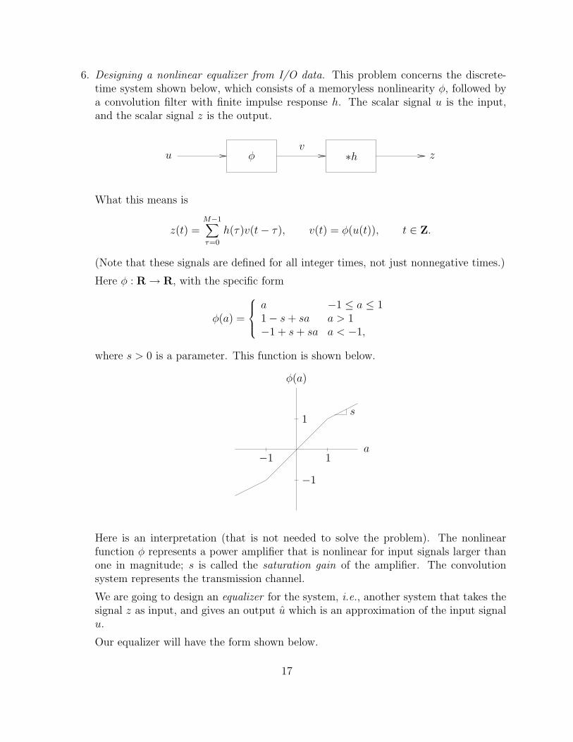
6. Designing a nonlinear equalizer from I/O data. This problem concerns the discrete-time system shown below, which consists of a memoryless nonlinearity φ, followed bya convolution filter with finite impulse response h. The scalar signal u is the input,and the scalar signal z is the output.

φ ∗huv

z

What this means is

z(t) =M−1∑

τ=0

h(τ)v(t− τ), v(t) = φ(u(t)), t ∈ Z.

(Note that these signals are defined for all integer times, not just nonnegative times.)

Here φ : R → R, with the specific form

φ(a) =

a −1 ≤ a ≤ 11 − s+ sa a > 1−1 + s+ sa a < −1,

where s > 0 is a parameter. This function is shown below.

1−1

φ(a)

a

1

−1

s

Here is an interpretation (that is not needed to solve the problem). The nonlinearfunction φ represents a power amplifier that is nonlinear for input signals larger thanone in magnitude; s is called the saturation gain of the amplifier. The convolutionsystem represents the transmission channel.

We are going to design an equalizer for the system, i.e., another system that takes thesignal z as input, and gives an output u which is an approximation of the input signalu.

Our equalizer will have the form shown below.

17

ψ∗g uv

z

This means

v(t) =M−1∑

τ=0

g(τ)z(t− τ), u(t) = ψ(v(t)), t ∈ Z.

This equalizer will work well provided g ∗ h ≈ δ (in which case v(t) ≈ v(t)), andψ = φ−1 (i.e., ψ(φ(a)) = a for all a).

To make sure our (standard) notation here is clear, recall that

(g ∗ h)(t) =min{M−1,t}

∑

τ=max{0,t−M+1}

g(τ)h(t− τ), t = 0, . . . , 2M − 1.

(Note: in matlab conv(g,h) gives the convolution of g and h, but these vectors areindexed from 1 to M , i.e., g(1) corresponds to g(0).) The term δ is the Kroneckerdelta, defined as δ(0) = 1, δ(i) = 0 for i 6= 0.

Now, finally, we come to the problem. You are given some input/output (I/O) datau(1), . . . , u(N), z(1), . . . , z(N), and M (the length of g, and also the length of h). Youdo not know the parameter s, or the channel impulse response h(0), . . . , h(M−1). Youalso don’t know u(t), z(t) for t ≤ 0.

(a) Explain how to find s, an estimate of the saturation gain s, and g(0), . . . , g(M−1),that minimize

J =1

N −M + 1

N∑

i=M

(

v(i) − φ(u(i)))2

.

Here u refers to the given input data, and v comes from the given output data z.Note that if g ∗ h = δ and s = s, we have J = 0.

We exclude i = 1, . . . ,M − 1 in the sum defining J because these terms depend(through v) on z(0), z(−1), . . ., which are unknown.

(b) Apply your method to the data given in the file nleq_data.m. Give the valuesof the parameters s and g(0), . . . , g(M − 1) found, as well as J . Plot g using thematlab command stem.

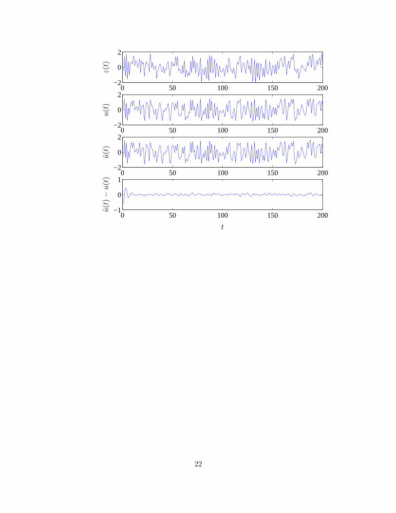
(c) Using the values of s and g(0), . . . , g(M − 1) found in part (b), find the equalizedsignal u(t), for t = 1, . . . , N . For the purposes of finding u(t) you can assumethat z(t) = 0 for t ≤ 0. As a result, we can expect a large equalization error (i.e.,u(t) − u(t)) for t = 1, . . . ,M − 1.

Plot the input signal u(t), the output signal z(t), the equalized signal u(t), andthe equalization error u(t) − u(t), for t = 1, . . . , N .

18

Solution.

(a) The estimate v(i) is a linear function of g, and φ(u(i)) is an affine function of s(i.e., linear plus a constant). Thus, the quantity

J =1

N −M + 1

N∑

i=M

(

v(i) − φ(u(i)))2

can be written as J = (1/(N −M + 1))‖y − Ax‖2, where

x = [g(M − 1) · · · g(0) s]T ,

yi =

1 u(i+M − 1) > 1−1 u(i+M − 1) < −1u(i+M − 1) otherwise,

for i = 1, . . . , N −M + 1, and

A =

z(1) · · · z(M) w1

.... . .

......

z(N −M + 1) · · · z(N) wN−M+1

,

where

wi =

1 − u(i+M − 1) u(i+M − 1) > 1−1 − u(i+M − 1) u(i+M − 1) < −10 otherwise,

for i = 1, . . . , N−M+1. Minimizing J is a least-squares problem and the solutionis given by

x = (ATA)−1ATy.

Several people used a method that gives very close to the correct solution, but ismore complicated than it needs to be, so we took off 5 or so points (dependingon the clarity). The method treats s as a parameter, not as a variable to bedetermined. For fixed s, we get a least-squares problem for g, which we solve.Then we have an out loop that sweeps over many values of s, to see which onehas the smallest objective value.

(b) The following matlab code implements the solution.

clear all

nleq_data;

% Forming least-squares problem

% x = [g(M-1) ... g(0) s]’

y = []; A = []; k = 0;

19

for i=M:N

k = k+1;

A(k,1:M) = z(i-M+1:i);

if u(i)>1

y(k,1) = 1;

A(k,M+1) = 1 - u(i);

elseif u(i) < -1

y(k,1) = -1;

A(k, M+1) = -1 - u(i);

else

y(k,1) = u(i);

A(k, M+1) = 0;

end

end

x = A\y;

g = flipud(x(1:M));

s = x(end);

fprintf(’\nSaturation gain estimate s hat = %f\n’, s);

J = (1/(N-M+1))*((norm(y - A*x))^2);

fprintf(’J = %e\n’, J);

vhat = conv(g,z);

uhat = [];

for i =1:length(vhat)

if vhat(i)>1

uhat(i,1) = (vhat(i)-1+s)/s;

elseif vhat(i) < -1

uhat(i,1) = (vhat(i)+1-s)/s;

else

uhat(i,1) = vhat(i);

end

end

The solution obtained is:

g

0 0.994895

1 0.198037

2 -0.351337

3 -0.339969

20

4 -0.062389

5 0.165468

6 0.150345

7 0.010682

8 -0.074457

9 -0.050343

Saturation gain estimate s hat = 0.500388

J = 1.200482e-03

0 1 2 3 4 5 6 7 8 9

−0.4

−0.2

0

0.2

0.4

0.6

0.8

1

i

g(i

)

(c) The input signal u(t), the output signal z(t), the equalized signal u(t) (assumingz(t) = 0, t ≤ 0), and the equalization error u(t)−u(t), for t = 1, . . . , N are shownbelow.

21

0 50 100 150 200−2

0

2

0 50 100 150 200−2

0

2

0 50 100 150 200−2

0

2

0 50 100 150 200−1

0

1

t

z(t)

u(t

)u(t

)u(t

)−u(t

)

22

7. A greedy control scheme. Our goal is to choose an input u : R+ → Rm, that is not toobig, and drives the state x : R+ → Rn of the system x = Ax+Bu to zero quickly. Todo this, we will choose u(t), for each t, to minimize the quantity

d

dt‖x(t)‖2 + ρ‖u(t)‖2,

where ρ > 0 is a given parameter. The first term gives the rate of decrease (if it isnegative) of the norm-squared of the state vector; the second term is a penalty forusing a large input.

This scheme is greedy because at each instant t, u(t) is chosen to minimize the com-positive objective above, without regard for the effects such an input might have inthe future.

(a) Show that u(t) can be expressed as u(t) = Kx(t), where K ∈ Rm×n. Give anexplicit formula for K. (In other words, the control scheme has the form of aconstant linear state feedback.)

(b) What are the conditions on A, B, and ρ under which we have (d/dt)‖x(t)‖2 < 0whenever x(t) 6= 0, using the scheme described above? (In other words, when doesthis control scheme result in the norm squared of the state always decreasing?)

(c) Find an example of a system (i.e., A and B), for which the open-loop systemx = Ax is stable, but the closed-loop system x = Ax + Bu (with u as above) isunstable, when ρ = 1. Try to find the simplest example you can, and be sure toshow us verification that the open-loop system is stable and that the closed-loopsystem is not. (We will not check this for you. You must explain how to checkthis, and attach code and associated output.)

Solution.

(a) We have

d

dt‖x(t)‖2 + ρ‖u(t)‖2 =

d

dt(x(t)Tx(t)) + ρ‖u(t)‖2

= x(t)Tx(t) + x(t)T x(t) + ρ‖u(t)‖2

= (Ax(t) +Bu(t))Tx(t) + x(t)T (Ax(t) +Bu(t)) + ρ‖u(t)‖2

= x(t)T (AT + A)x(t) + 2x(t)TBu(t) + ρ‖u(t)‖2.

To minimize this with respect to u(t), we set the gradient equal to zero:

2BTx(t) + 2ρu(t) = 0.

This yields u(t) = Kx(t), with K = −(1/ρ)BT .

For use in part (c), we note that the closed-loop dynamics are given by

x = Ax+Bu = (A− (1/ρ)BBT )x.

23

(b) With this value of u(t), we have

d

dt‖x(t)‖2 = x(t)T

(

AT + A− (2/ρ)BBT)

x(t).

This is negative for all nonzero x(t) if and only if the matrix in the quadratic formis negative definite, i.e.,

AT + A− (2/ρ)BBT ≺ 0.

There are many other ways to write this condition.

(c) We can’t find an example with n = 1, but for n = 2 we can use

A =

[

−0.1 10 −0.1

]

B =

[

1−1

]

, ρ = 1.

Clearly A has negative eigenvalues and therefore the open-loop is stable but asthe following Matlab code shows, the closed-loop system is unstable. The Matlabcode is

A=[-0.1 1; 0 -0.1];

B=[1 -1]’;

rho=1;

eig(A)

eig(A-(1/rho)*B*B’)

The output of the above code is

ans =

-0.1000

-0.1000

ans =

0.3142

-2.5142.

24