final case study churn (autosaved)
TRANSCRIPT

FINAL CASE STUDY12/08/2016
Pothireddy Marreddy
Mobicom is concerned that the market environment of rising churn rates and declining ARPU will hit them even harder as churn rate at Mobicom is relatively high. Currently they have been focusing on retaining their customers on a reactive basis when the subscriber calls in to close the account
Objective: What are the top five factors driving likelihood of churn at Mobicom Roll out targeted proactive retention programs, which include usage enhancing marketing
programs to increase minutes of usage (MOU), rate plan migration, and a bundling strategy among others.
Key Attributes
The Internet and recommendation of family and friends.
falling ARPU
Usage based promotions to increase minutes of usage (MOU) for both voice and data
Bundling
Optimal rate plan
Artificial churn/spinners or serial churners
Top Line Questions of Interest to Senior Management:
1. What are the top five factors driving likelihood of churn at Mobicom?
2. Validation of survey findings. a) Whether “cost and billing” and “network and service quality”
are important factors influencing churn behavior. b) Are data usage connectivity issues turning
out to be costly? In other words, is it leading to churn?
3. Would you recommend rate plan migration as a proactive retention strategy?
4. What would be your recommendation on how to use this churn model for prioritization of
customers for a proactive retention campaigns in the future?
/* create a permanent library name*/
Libname final "Y:\Programes\SAS Graded Assignment\Final Case Study";run;
/*Import the dataset*/

Proc import datafile = "Z:\Assignments\Graded Assignment\Topic 13 - Final Case Study Implementation/telecomfinal.csv"DBMS = CSV OUT = final.telecom replace;DATAROW = 2;GUESSINGROWS = 2000;GETNAMES = YES;Mixed = yes;SCANTEXT = Yes;RUN;
DATA EXPLORATION:
/*understand the data what is contained*/Proc contents data = final.telecom;run;
Data set "FINAL.telecom" has 66297 observation(s) and 79 variable(s) -Among 45 variables are character in nature and 34 are numeric variables-Need to convert the character variables to into numeric variables by creating dummy variables and buckets/bins for the range variables
/*check if there are any missing values and statistical analysis*/proc means data = final.telecom N NMISS MEAN STD MIN MAX MODE MEDIAN;run;
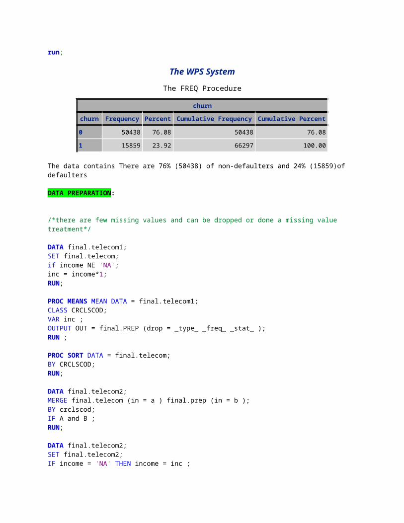
/*check how many are dafaulters*/proc freq data = final.telecom;table churn;run;
The WPS SystemThe FREQ Procedure
churnchurn Frequency Percent Cumulative
FrequencyCumulative Percent
0 50438 76.08 50438 76.081 15859 23.92 66297 100.00
The data contains There are 76% (50438) of non-defaulters and 24% (15859)of defaulters
DATA PREPARATION:
/*there are few missing values and can be dropped or done a missing value treatment*/
DATA final.telecom1;SET final.telecom;if income NE 'NA';inc = income*1;RUN;
PROC MEANS MEAN DATA = final.telecom1;CLASS CRCLSCOD;VAR inc ;OUTPUT OUT = final.PREP (drop = _type_ _freq_ _stat_ );RUN ;
PROC SORT DATA = final.telecom;BY CRCLSCOD;RUN;
DATA final.telecom2;MERGE final.telecom (in = a ) final.prep (in = b );BY crclscod;IF A and B ;RUN;
DATA final.telecom2;SET final.telecom2;IF income = 'NA' THEN income = inc ;new_income = income * 1 ;RUN;
/*converting character variables into numeric variables*/
DATA final.telecom2;SET final.telecom2;
/* create income bucket based on quartile values */
IF new_income LE 4.9 THEN income_bkt = 1;ELSE IF new_income LE 6 THEN income_bkt = 2;ELSE IF new_income LE 7 THEN income_bkt = 3;ELSE income_bkt = 4 ;
/* create bucket for callwait based on quartile values */
IF callwait_mean LE 0 then callwait_bkt = 1 ;ELSE IF callwait_mean LE 0.334 THEN callwait_bkt = 2;ELSE IF callwait_mean LE 1.67 THEN callwait_bkt = 3;ELSE callwait_bkt = 4;
/* create an indicator variable for roaming */
IF ROAM_MEAN > 0 THEN roam_ind = 1 ;ELSE roam_ind = 0 ;
/* create drop or block calls buckets using quartile values */
IF DROP_BLK_MEAN LE 1.67 THEN drop_blk_bkt = 1 ;ELSE IF DROP_BLK_MEAN LE 5.34 THEN drop_blk_bkt = 2;ELSE IF DROP_BLK_MEAN LE 12.67 THEN drop_blk_bkt = 3;ELSE drop_blk_bkt = 4;
/* create buckets for placed voie calls using quartile values */
IF PLCD_VCE_MEAN LE 40.67 THEN PLCD_VCE_bkt = 1 ;
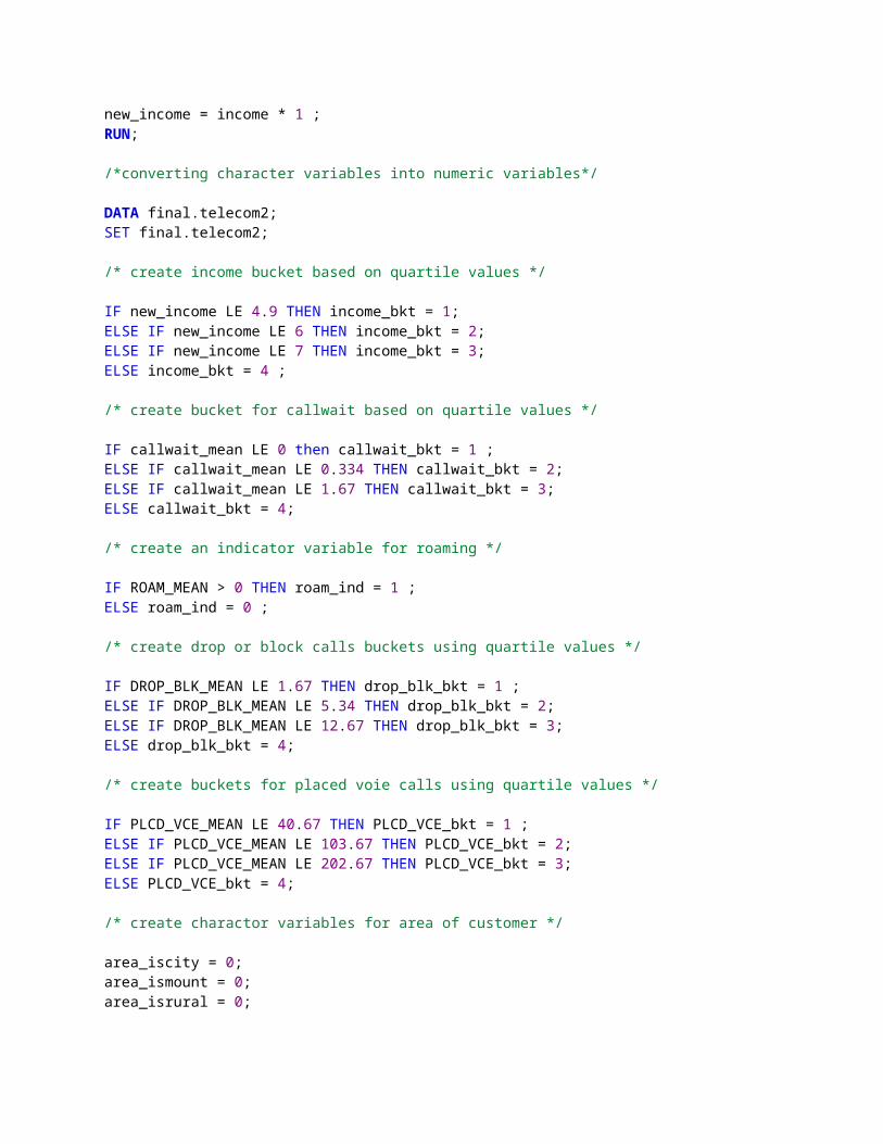
ELSE IF PLCD_VCE_MEAN LE 103.67 THEN PLCD_VCE_bkt = 2;ELSE IF PLCD_VCE_MEAN LE 202.67 THEN PLCD_VCE_bkt = 3;ELSE PLCD_VCE_bkt = 4;
/* create charactor variables for area of customer */
area_iscity = 0;area_ismount = 0;area_isrural = 0;
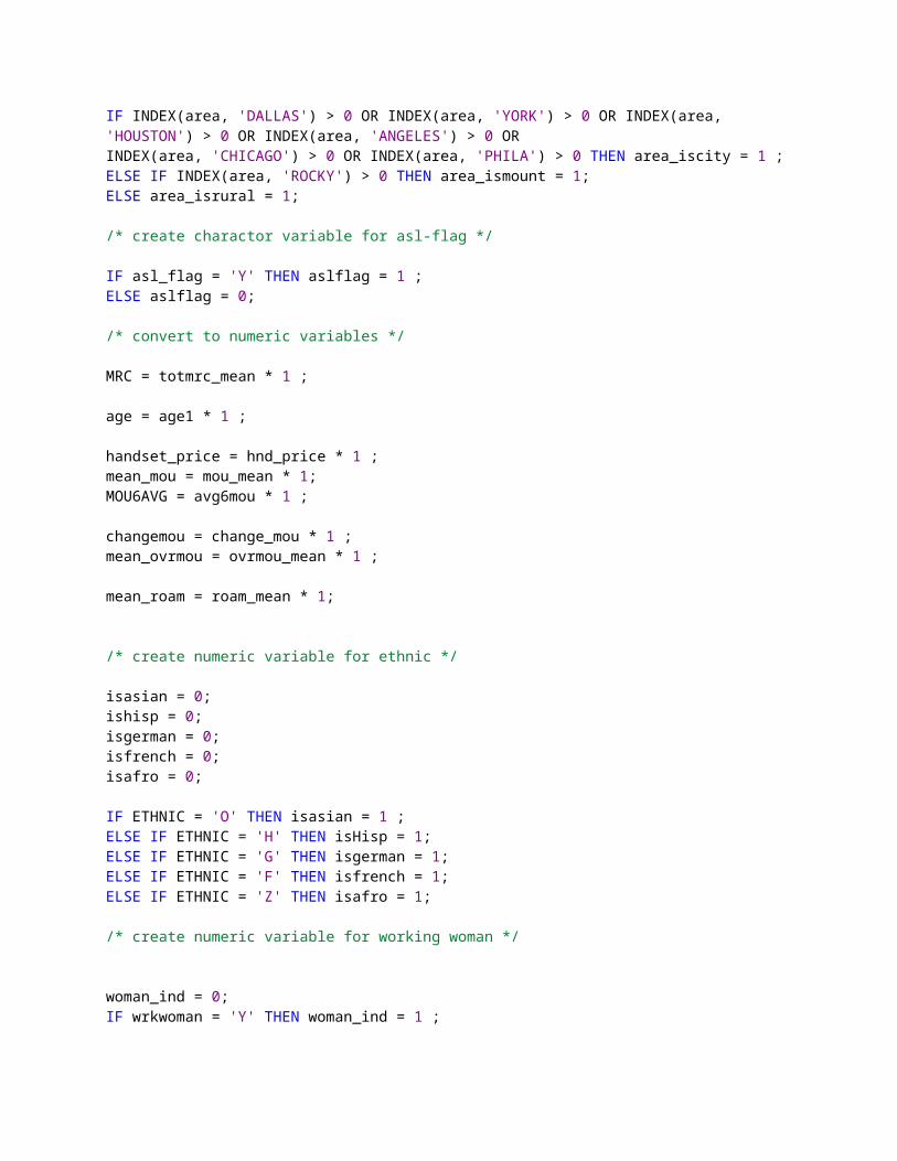
IF INDEX(area, 'DALLAS') > 0 OR INDEX(area, 'YORK') > 0 OR INDEX(area, 'HOUSTON') > 0 OR INDEX(area, 'ANGELES') > 0 ORINDEX(area, 'CHICAGO') > 0 OR INDEX(area, 'PHILA') > 0 THEN area_iscity = 1 ;ELSE IF INDEX(area, 'ROCKY') > 0 THEN area_ismount = 1;ELSE area_isrural = 1;
/* create charactor variable for asl-flag */
IF asl_flag = 'Y' THEN aslflag = 1 ;ELSE aslflag = 0;
/* convert to numeric variables */
MRC = totmrc_mean * 1 ;
age = age1 * 1 ;
handset_price = hnd_price * 1 ;mean_mou = mou_mean * 1;MOU6AVG = avg6mou * 1 ;
changemou = change_mou * 1 ;mean_ovrmou = ovrmou_mean * 1 ;
mean_roam = roam_mean * 1;
/* create numeric variable for ethnic */
isasian = 0;ishisp = 0;isgerman = 0;isfrench = 0;isafro = 0;
IF ETHNIC = 'O' THEN isasian = 1 ;ELSE IF ETHNIC = 'H' THEN isHisp = 1;ELSE IF ETHNIC = 'G' THEN isgerman = 1;ELSE IF ETHNIC = 'F' THEN isfrench = 1;ELSE IF ETHNIC = 'Z' THEN isafro = 1;
/* create numeric variable for working woman */
woman_ind = 0;IF wrkwoman = 'Y' THEN woman_ind = 1 ;
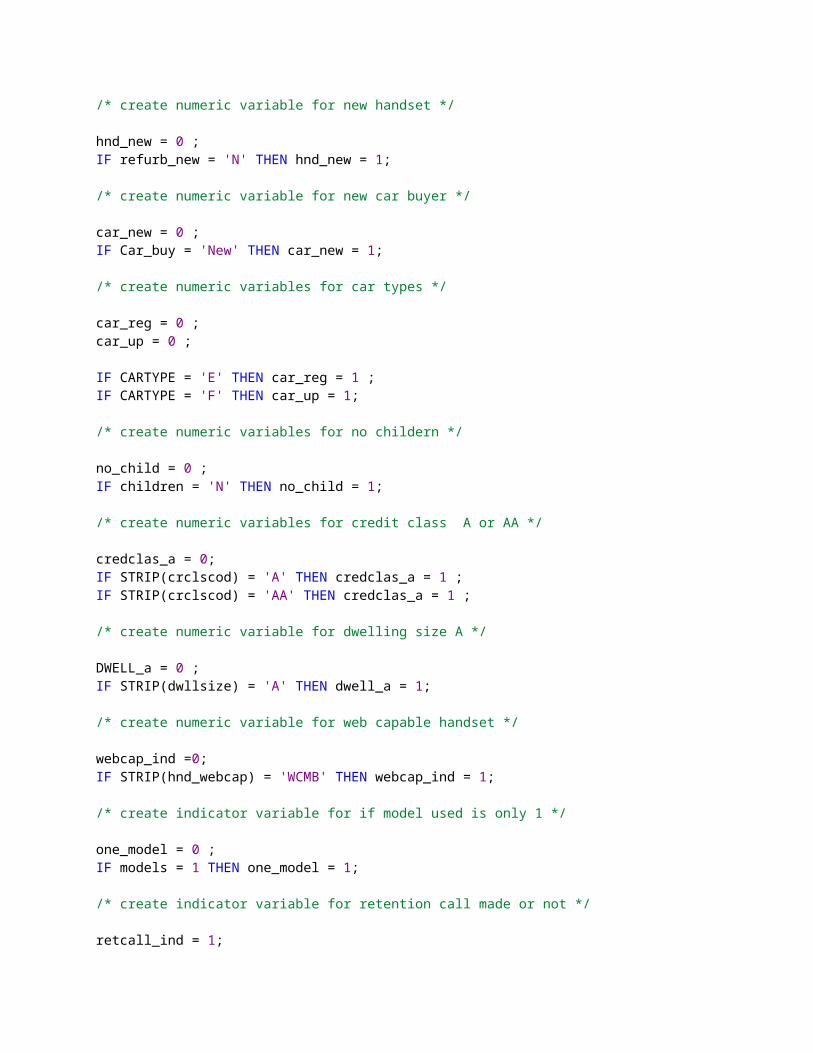
/* create numeric variable for new handset */
hnd_new = 0 ;IF refurb_new = 'N' THEN hnd_new = 1;
/* create numeric variable for new car buyer */
car_new = 0 ;IF Car_buy = 'New' THEN car_new = 1;
/* create numeric variables for car types */
car_reg = 0 ;car_up = 0 ;
IF CARTYPE = 'E' THEN car_reg = 1 ;IF CARTYPE = 'F' THEN car_up = 1;
/* create numeric variables for no childern */
no_child = 0 ;IF children = 'N' THEN no_child = 1;
/* create numeric variables for credit class A or AA */
credclas_a = 0;IF STRIP(crclscod) = 'A' THEN credclas_a = 1 ;IF STRIP(crclscod) = 'AA' THEN credclas_a = 1 ;
/* create numeric variable for dwelling size A */
DWELL_a = 0 ;IF STRIP(dwllsize) = 'A' THEN dwell_a = 1;
/* create numeric variable for web capable handset */
webcap_ind =0;IF STRIP(hnd_webcap) = 'WCMB' THEN webcap_ind = 1;
/* create indicator variable for if model used is only 1 */
one_model = 0 ;IF models = 1 THEN one_model = 1;
/* create indicator variable for retention call made or not */
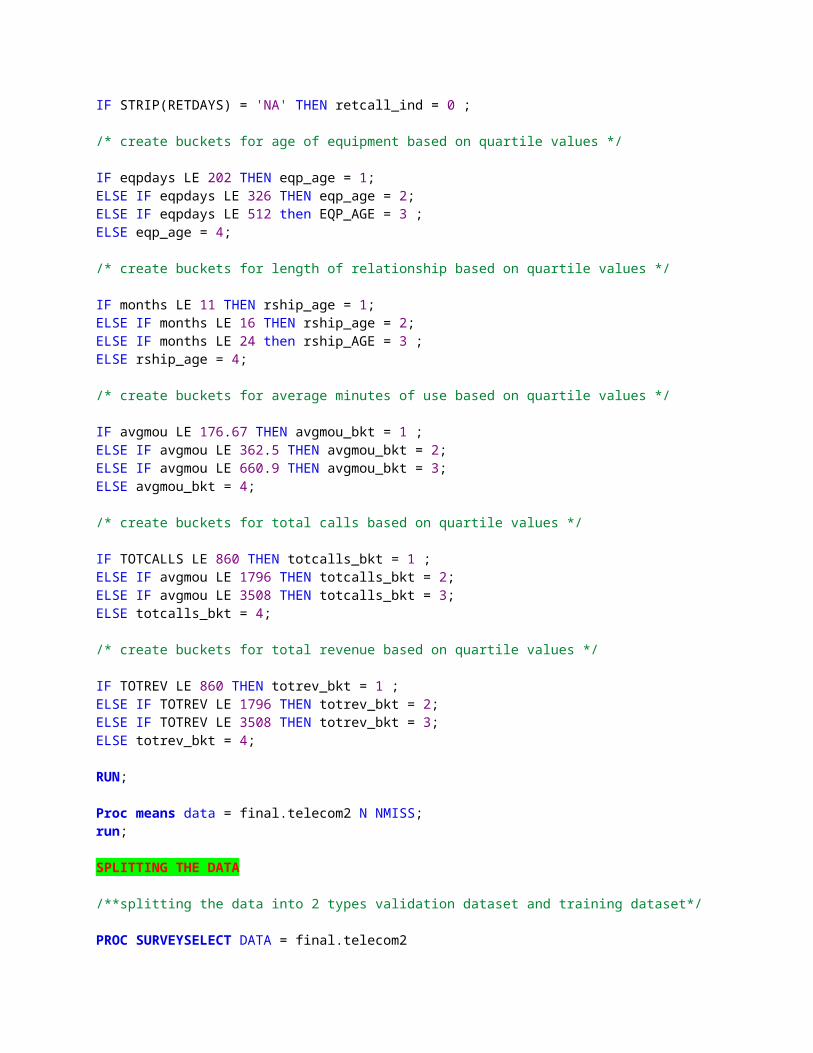
retcall_ind = 1;IF STRIP(RETDAYS) = 'NA' THEN retcall_ind = 0 ;
/* create buckets for age of equipment based on quartile values */
IF eqpdays LE 202 THEN eqp_age = 1;ELSE IF eqpdays LE 326 THEN eqp_age = 2;ELSE IF eqpdays LE 512 then EQP_AGE = 3 ;ELSE eqp_age = 4;
/* create buckets for length of relationship based on quartile values */
IF months LE 11 THEN rship_age = 1;ELSE IF months LE 16 THEN rship_age = 2;ELSE IF months LE 24 then rship_AGE = 3 ;ELSE rship_age = 4;
/* create buckets for average minutes of use based on quartile values */
IF avgmou LE 176.67 THEN avgmou_bkt = 1 ;ELSE IF avgmou LE 362.5 THEN avgmou_bkt = 2;ELSE IF avgmou LE 660.9 THEN avgmou_bkt = 3;ELSE avgmou_bkt = 4;
/* create buckets for total calls based on quartile values */
IF TOTCALLS LE 860 THEN totcalls_bkt = 1 ;ELSE IF avgmou LE 1796 THEN totcalls_bkt = 2;ELSE IF avgmou LE 3508 THEN totcalls_bkt = 3;ELSE totcalls_bkt = 4;
/* create buckets for total revenue based on quartile values */
IF TOTREV LE 860 THEN totrev_bkt = 1 ;ELSE IF TOTREV LE 1796 THEN totrev_bkt = 2;ELSE IF TOTREV LE 3508 THEN totrev_bkt = 3;ELSE totrev_bkt = 4;
RUN;
Proc means data = final.telecom2 N NMISS;run;
SPLITTING THE DATA
/**splitting the data into 2 types validation dataset and training dataset*/
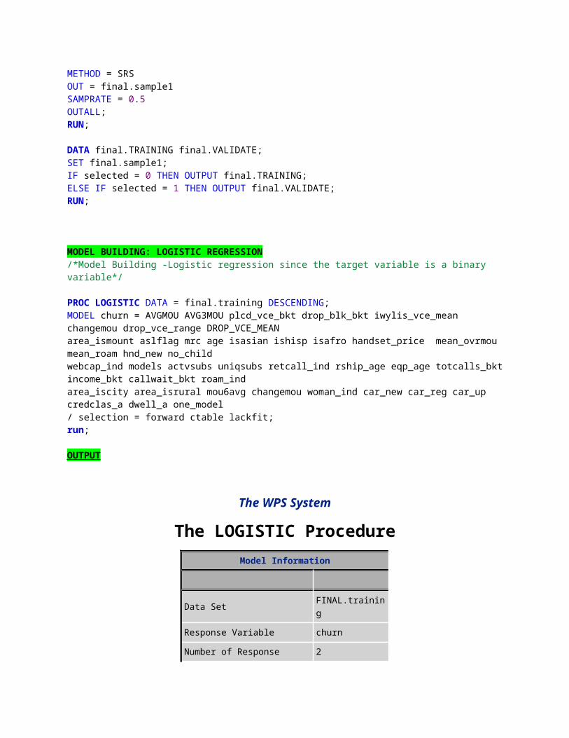
PROC SURVEYSELECT DATA = final.telecom2METHOD = SRSOUT = final.sample1SAMPRATE = 0.5OUTALL;RUN;
DATA final.TRAINING final.VALIDATE;SET final.sample1;IF selected = 0 THEN OUTPUT final.TRAINING;ELSE IF selected = 1 THEN OUTPUT final.VALIDATE;RUN;
MODEL BUILDING: LOGISTIC REGRESSION/*Model Building -Logistic regression since the target variable is a binary variable*/
PROC LOGISTIC DATA = final.training DESCENDING;
MODEL churn = AVGMOU AVG3MOU plcd_vce_bkt drop_blk_bkt iwylis_vce_mean changemou drop_vce_range DROP_VCE_MEAN area_ismount aslflag mrc age isasian ishisp isafro handset_price mean_ovrmou mean_roam hnd_new no_child webcap_ind models actvsubs uniqsubs retcall_ind rship_age eqp_age totcalls_bkt income_bkt callwait_bkt roam_ind area_iscity area_isrural mou6avg changemou woman_ind car_new car_reg car_up credclas_a dwell_a one_model / selection = forward ctable lackfit;run;
OUTPUT
The WPS System
The LOGISTIC ProcedureModel Information
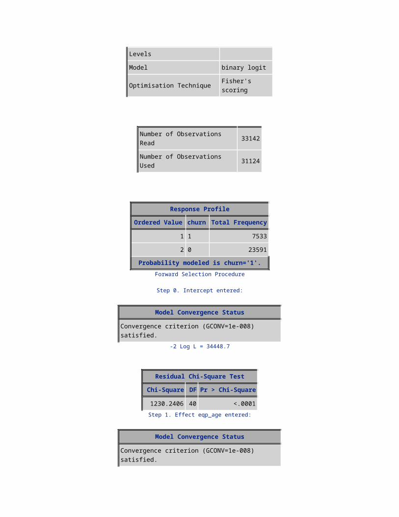
Data Set FINAL.trainingResponse Variable churnNumber of Response Levels 2Model binary logitOptimisation Technique Fisher's scoring
Number of Observations Read 33142Number of Observations Used 31124
Response ProfileOrdered Value churn Total
Frequency
1 1 75332 0 23591
Probability modeled is churn='1'.Forward Selection Procedure
Step 0. Intercept entered:
Model Convergence Status
Convergence criterion (GCONV=1e-008) satisfied.-2 Log L = 34448.7
Residual Chi-Square Test
Chi-Square DF Pr > Chi-Square
1230.2406 40 <.0001Step 1. Effect eqp_age entered:
Model Convergence Status
Convergence criterion (GCONV=1e-008) satisfied.
Model Fit StatisticsCriterion Intercept only Intercept and Covariates
AIC 34450.711 34053.568SC 34459.057 34070.259-2 Log L 34448.711 34049.568
Testing Global Null Hypothesis: BETA=0Test Chi-Square DF Pr > Chi-Square
Likelihood Ratio 399.1436 1 <.0001Score 395.7067 1 <.0001Wald 391.0589 1 <.0001
Residual Chi-Square TestChi-Square DF Pr > Chi-Square
869.4213 39 <.0001Step 2. Effect retcall_ind entered:
Model Convergence Status
Convergence criterion (GCONV=1e-008) satisfied.
Model Fit StatisticsCriterion Intercept only Intercept and Covariates
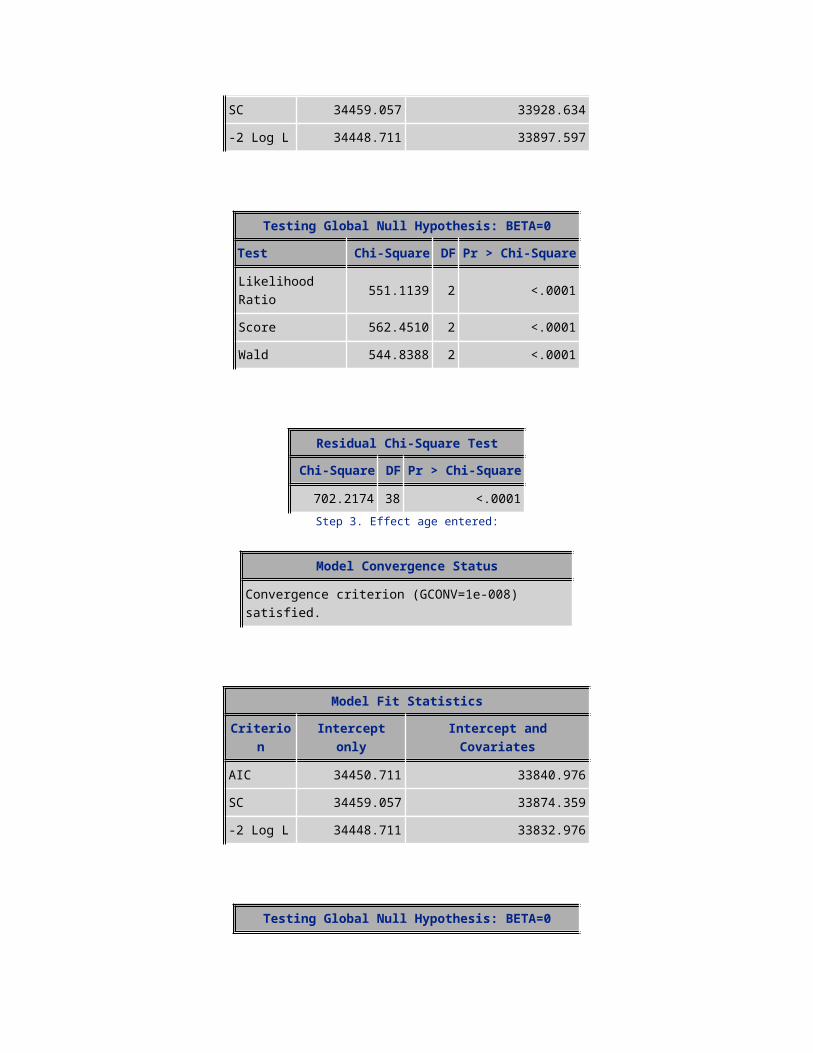
AIC 34450.711 33903.597SC 34459.057 33928.634-2 Log L 34448.711 33897.597
Testing Global Null Hypothesis: BETA=0Test Chi-Square DF Pr > Chi-Square
Likelihood Ratio 551.1139 2 <.0001Score 562.4510 2 <.0001Wald 544.8388 2 <.0001
Residual Chi-Square TestChi-Square DF Pr > Chi-Square
702.2174 38 <.0001Step 3. Effect age entered:
Model Convergence Status
Convergence criterion (GCONV=1e-008) satisfied.
Model Fit StatisticsCriterion Intercept only Intercept and Covariates
AIC 34450.711 33840.976SC 34459.057 33874.359-2 Log L 34448.711 33832.976
Testing Global Null Hypothesis: BETA=0Test Chi-Square DF Pr > Chi-Square

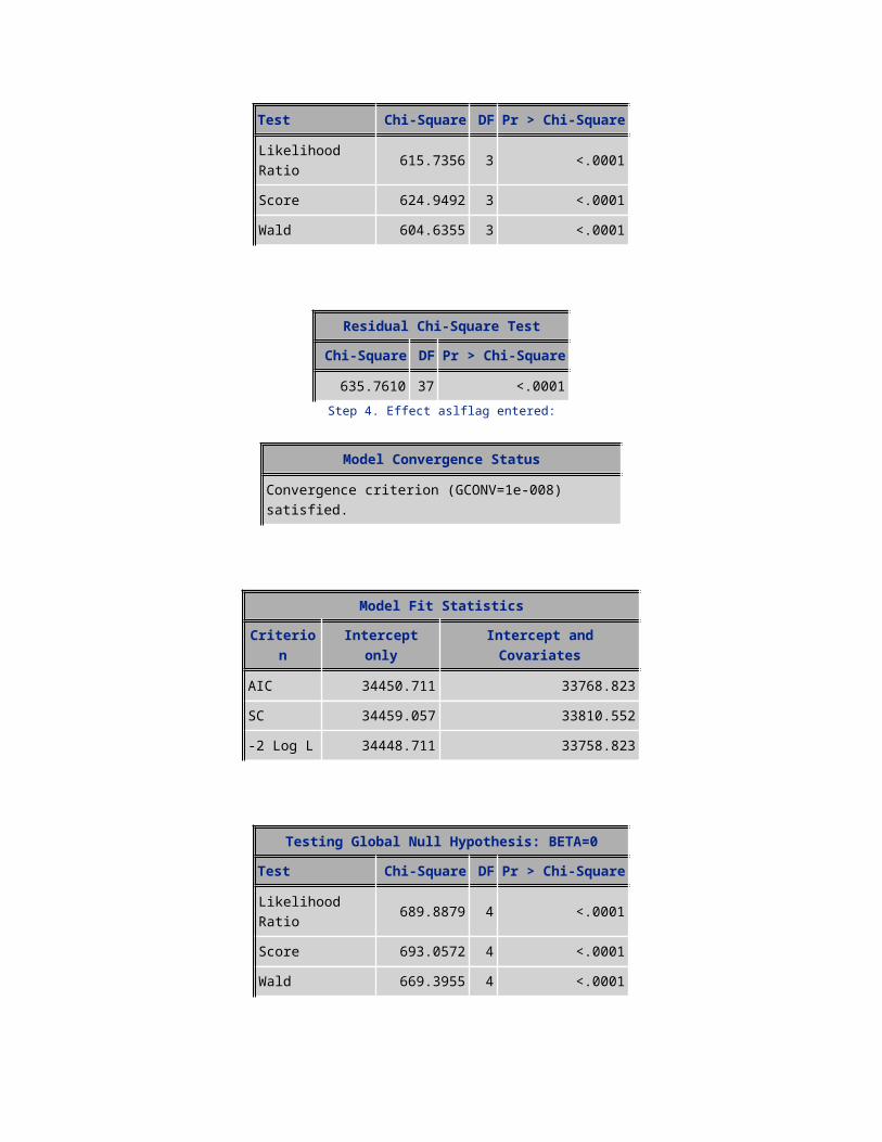
Likelihood Ratio 615.7356 3 <.0001Score 624.9492 3 <.0001Wald 604.6355 3 <.0001
Residual Chi-Square TestChi-Square DF Pr > Chi-Square
635.7610 37 <.0001Step 4. Effect aslflag entered:
Model Convergence Status
Convergence criterion (GCONV=1e-008) satisfied.
Model Fit StatisticsCriterion Intercept only Intercept and Covariates
AIC 34450.711 33768.823SC 34459.057 33810.552-2 Log L 34448.711 33758.823
Testing Global Null Hypothesis: BETA=0Test Chi-Square DF Pr > Chi-Square
Likelihood Ratio 689.8879 4 <.0001Score 693.0572 4 <.0001Wald 669.3955 4 <.0001
Residual Chi-Square TestChi-Square DF Pr > Chi-Square
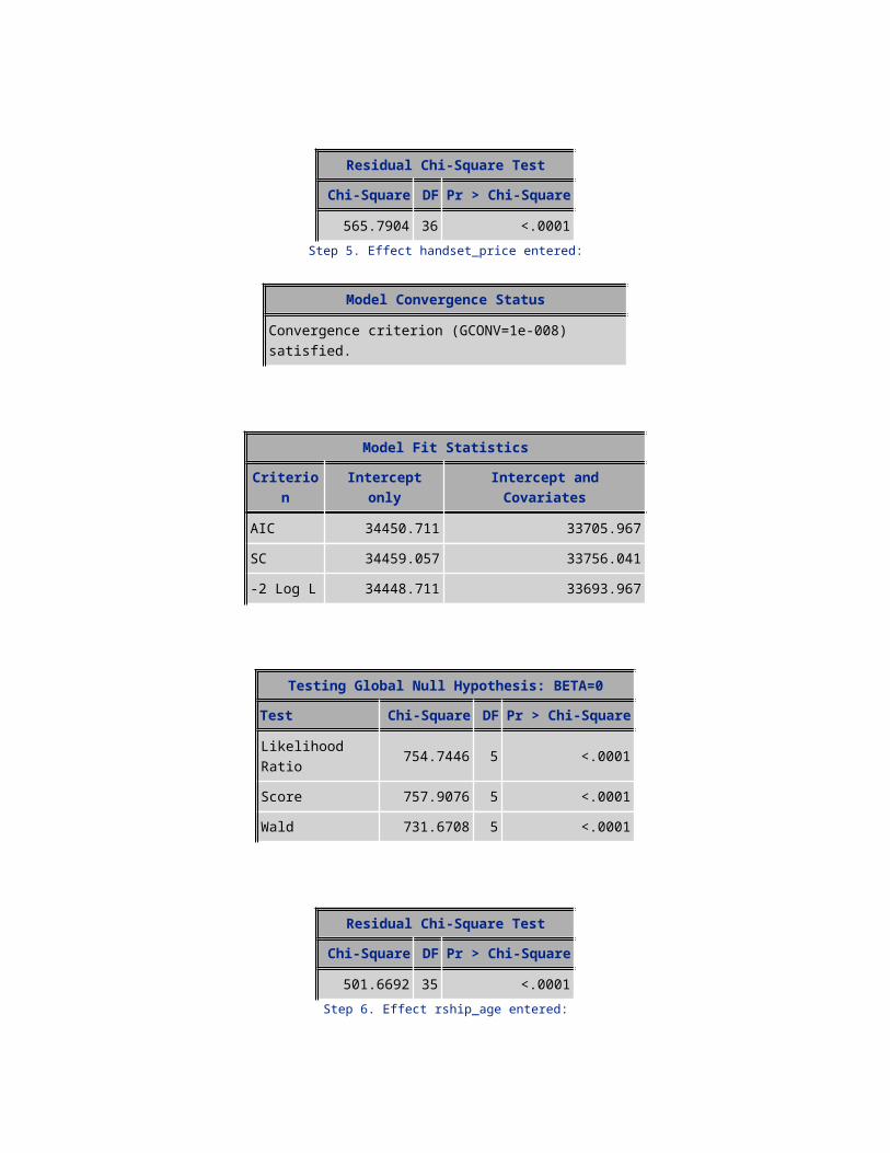
565.7904 36 <.0001Step 5. Effect handset_price entered:
Model Convergence Status
Convergence criterion (GCONV=1e-008) satisfied.
Model Fit StatisticsCriterion Intercept only Intercept and Covariates
AIC 34450.711 33705.967SC 34459.057 33756.041-2 Log L 34448.711 33693.967
Testing Global Null Hypothesis: BETA=0Test Chi-Square DF Pr > Chi-Square
Likelihood Ratio 754.7446 5 <.0001Score 757.9076 5 <.0001Wald 731.6708 5 <.0001
Residual Chi-Square TestChi-Square DF Pr > Chi-Square
501.6692 35 <.0001Step 6. Effect rship_age entered:
Model Convergence Status
Convergence criterion (GCONV=1e-008) satisfied.
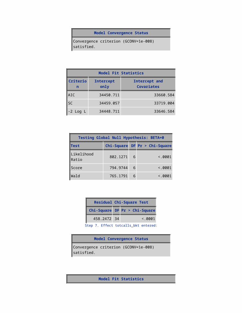
Model Fit StatisticsCriterion Intercept only Intercept and Covariates
AIC 34450.711 33660.584SC 34459.057 33719.004-2 Log L 34448.711 33646.584
Testing Global Null Hypothesis: BETA=0Test Chi-Square DF Pr > Chi-Square
Likelihood Ratio 802.1271 6 <.0001Score 794.9744 6 <.0001Wald 765.1791 6 <.0001
Residual Chi-Square TestChi-Square DF Pr > Chi-Square
458.2472 34 <.0001Step 7. Effect totcalls_bkt entered:
Model Convergence Status
Convergence criterion (GCONV=1e-008) satisfied.
Model Fit StatisticsCriterion Intercept only Intercept and Covariates
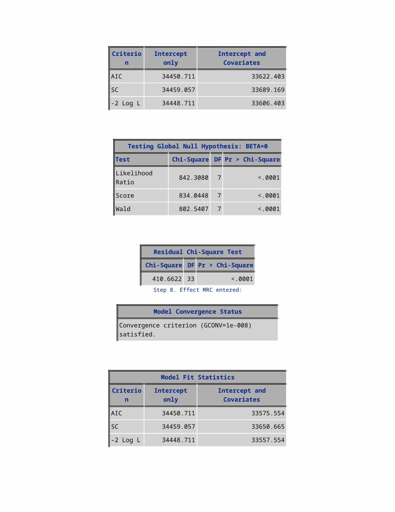
AIC 34450.711 33622.403SC 34459.057 33689.169-2 Log L 34448.711 33606.403
Testing Global Null Hypothesis: BETA=0Test Chi-Square DF Pr > Chi-Square
Likelihood Ratio 842.3080 7 <.0001Score 834.0448 7 <.0001Wald 802.5407 7 <.0001
Residual Chi-Square TestChi-Square DF Pr > Chi-Square
410.6622 33 <.0001Step 8. Effect MRC entered:
Model Convergence Status
Convergence criterion (GCONV=1e-008) satisfied.
Model Fit StatisticsCriterion Intercept only Intercept and Covariates
AIC 34450.711 33575.554SC 34459.057 33650.665-2 Log L 34448.711 33557.554
Testing Global Null Hypothesis: BETA=0Test Chi-Square DF Pr > Chi-Square
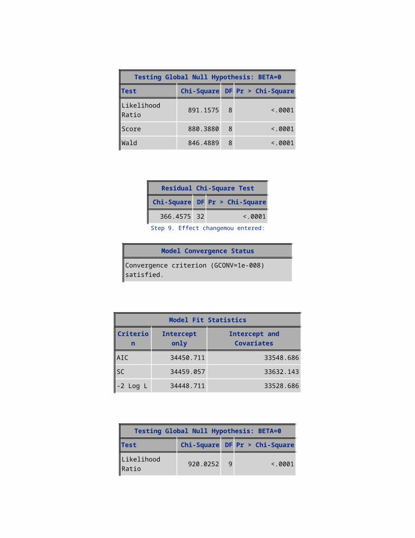
Likelihood Ratio 891.1575 8 <.0001Score 880.3880 8 <.0001Wald 846.4889 8 <.0001
Residual Chi-Square TestChi-Square DF Pr > Chi-Square
366.4575 32 <.0001Step 9. Effect changemou entered:
Model Convergence Status
Convergence criterion (GCONV=1e-008) satisfied.
Model Fit StatisticsCriterion Intercept only Intercept and Covariates
AIC 34450.711 33548.686SC 34459.057 33632.143-2 Log L 34448.711 33528.686
Testing Global Null Hypothesis: BETA=0Test Chi-Square DF Pr > Chi-Square
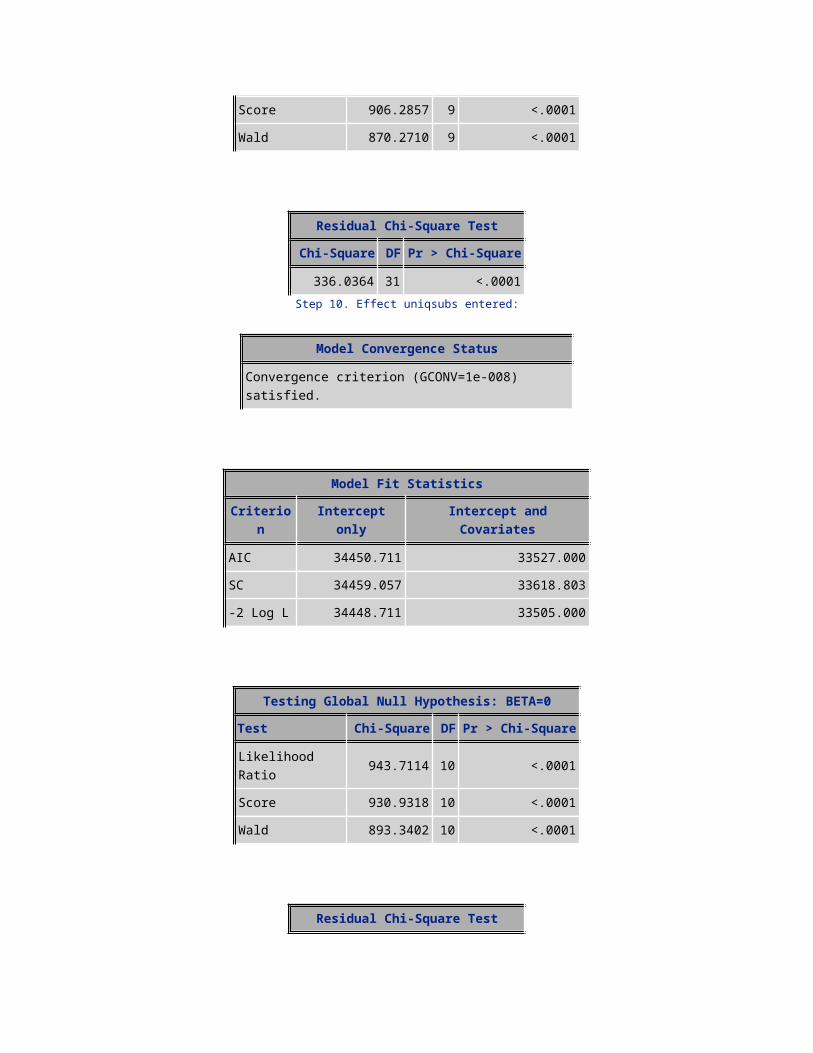
Likelihood Ratio 920.0252 9 <.0001Score 906.2857 9 <.0001Wald 870.2710 9 <.0001
Residual Chi-Square TestChi-Square DF Pr > Chi-Square
336.0364 31 <.0001Step 10. Effect uniqsubs entered:
Model Convergence Status
Convergence criterion (GCONV=1e-008) satisfied.
Model Fit StatisticsCriterion Intercept only Intercept and Covariates
AIC 34450.711 33527.000SC 34459.057 33618.803-2 Log L 34448.711 33505.000
Testing Global Null Hypothesis: BETA=0Test Chi-Square DF Pr > Chi-Square
Likelihood Ratio 943.7114 10 <.0001Score 930.9318 10 <.0001Wald 893.3402 10 <.0001
Residual Chi-Square TestChi-Square DF Pr > Chi-Square
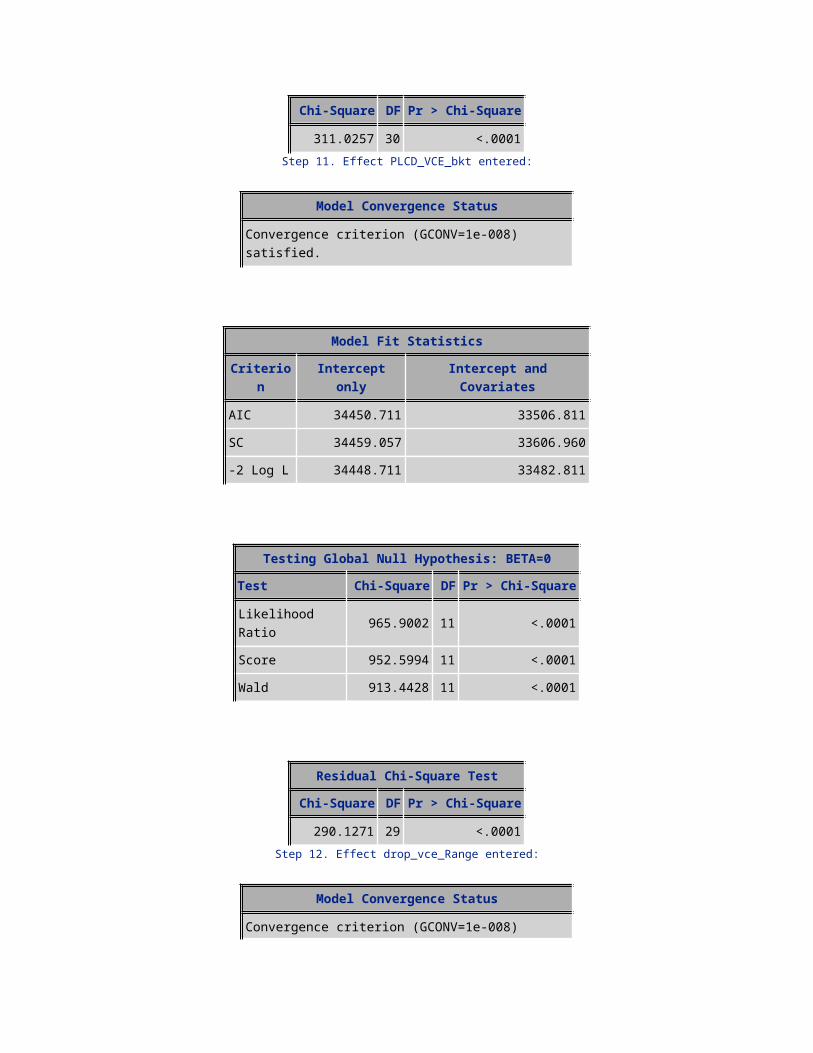
311.0257 30 <.0001Step 11. Effect PLCD_VCE_bkt entered:
Model Convergence Status
Convergence criterion (GCONV=1e-008) satisfied.
Model Fit StatisticsCriterion Intercept only Intercept and Covariates
AIC 34450.711 33506.811SC 34459.057 33606.960-2 Log L 34448.711 33482.811
Testing Global Null Hypothesis: BETA=0Test Chi-Square DF Pr > Chi-Square
Likelihood Ratio 965.9002 11 <.0001Score 952.5994 11 <.0001Wald 913.4428 11 <.0001
Residual Chi-Square TestChi-Square DF Pr > Chi-Square
290.1271 29 <.0001Step 12. Effect drop_vce_Range entered:
Model Convergence Status
Convergence criterion (GCONV=1e-008) satisfied.
Model Fit StatisticsCriterion Intercept only Intercept and Covariates
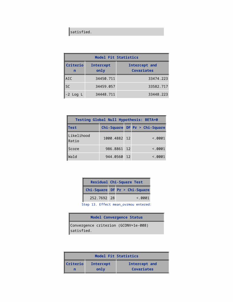
AIC 34450.711 33474.223SC 34459.057 33582.717
-2 Log L 34448.711 33448.223
Testing Global Null Hypothesis: BETA=0Test Chi-Square DF Pr > Chi-Square
Likelihood Ratio 1000.4882 12 <.0001Score 986.8861 12 <.0001Wald 944.0560 12 <.0001
Residual Chi-Square TestChi-Square DF Pr > Chi-Square
252.7692 28 <.0001Step 13. Effect mean_ovrmou entered:
Model Convergence Status
Convergence criterion (GCONV=1e-008) satisfied.
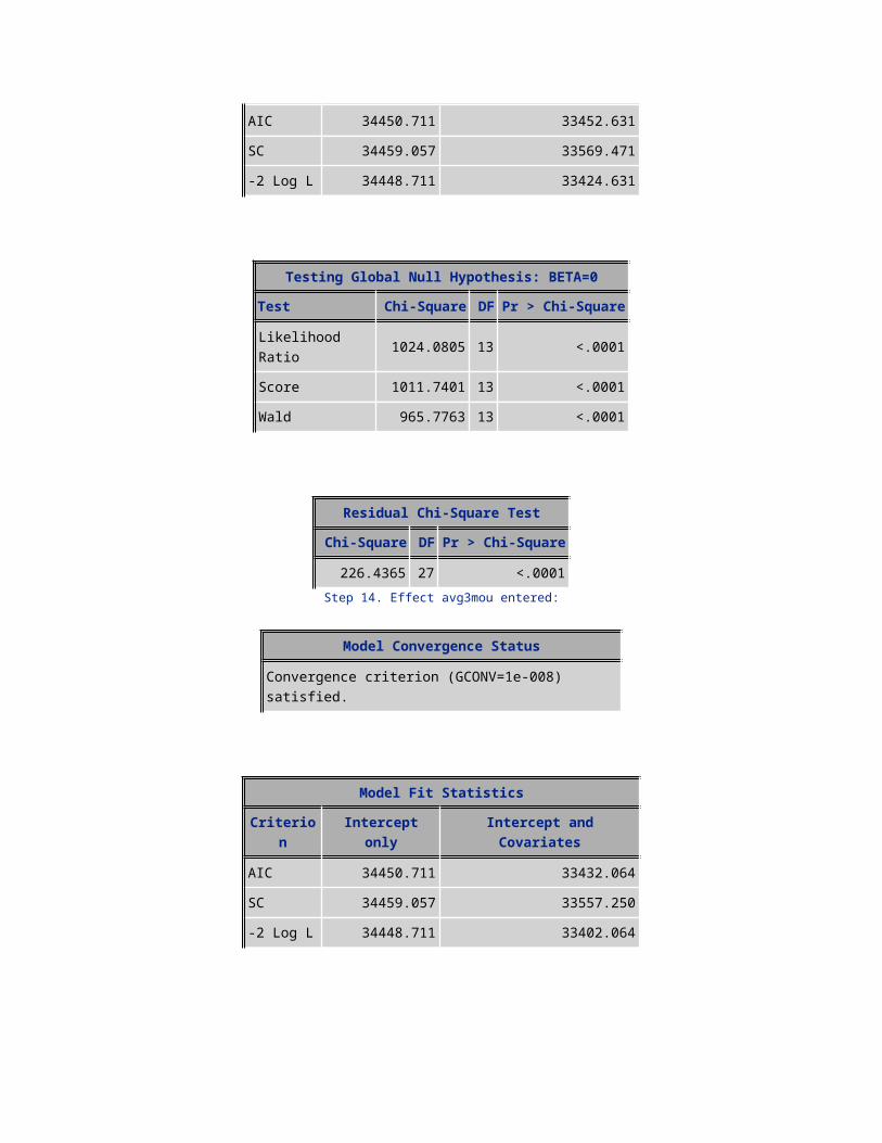
Model Fit StatisticsCriterion Intercept only Intercept and Covariates
AIC 34450.711 33452.631SC 34459.057 33569.471-2 Log L 34448.711 33424.631
Testing Global Null Hypothesis: BETA=0Test Chi-Square DF Pr > Chi-Square
Likelihood Ratio 1024.0805 13 <.0001Score 1011.7401 13 <.0001Wald 965.7763 13 <.0001
Residual Chi-Square TestChi-Square DF Pr > Chi-Square
226.4365 27 <.0001Step 14. Effect avg3mou entered:
Model Convergence Status
Convergence criterion (GCONV=1e-008) satisfied.
Model Fit StatisticsCriterion Intercept only Intercept and Covariates
AIC 34450.711 33432.064SC 34459.057 33557.250-2 Log L 34448.711 33402.064
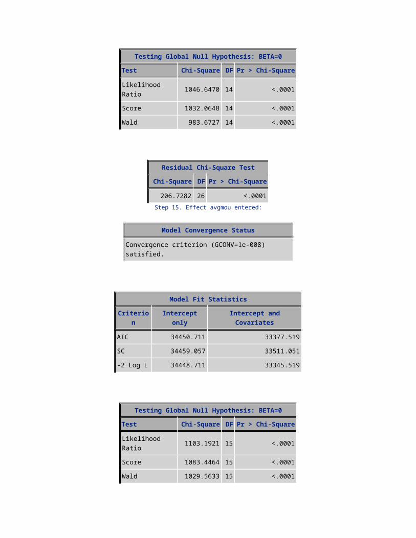
Testing Global Null Hypothesis: BETA=0Test Chi-Square DF Pr > Chi-Square
Likelihood Ratio 1046.6470 14 <.0001Score 1032.0648 14 <.0001Wald 983.6727 14 <.0001
Residual Chi-Square TestChi-Square DF Pr > Chi-Square
206.7282 26 <.0001Step 15. Effect avgmou entered:
Model Convergence Status
Convergence criterion (GCONV=1e-008) satisfied.
Model Fit StatisticsCriterion Intercept only Intercept and Covariates
AIC 34450.711 33377.519SC 34459.057 33511.051-2 Log L 34448.711 33345.519
Testing Global Null Hypothesis: BETA=0Test Chi-Square DF Pr > Chi-Square
Likelihood Ratio 1103.1921 15 <.0001Score 1083.4464 15 <.0001Wald 1029.5633 15 <.0001
Residual Chi-Square TestChi-Square DF Pr > Chi-Square
151.0034 25 <.0001Step 16. Effect isafro entered:
Model Convergence Status
Convergence criterion (GCONV=1e-008) satisfied.
Model Fit StatisticsCriterion Intercept only Intercept and Covariates
AIC 34450.711 33356.790SC 34459.057 33498.668-2 Log L 34448.711 33322.790
Testing Global Null Hypothesis: BETA=0Test Chi-Square DF Pr > Chi-Square
Likelihood Ratio 1125.9208 16 <.0001Score 1103.2109 16 <.0001Wald 1047.7040 16 <.0001
Residual Chi-Square TestChi-Square DF Pr > Chi-Square
129.2814 24 <.0001Step 17. Effect hnd_new entered:
Model Convergence Status
Convergence criterion (GCONV=1e-008) satisfied.
Model Fit StatisticsCriterion Intercept only Intercept and Covariates
AIC 34450.711 33344.370SC 34459.057 33494.593-2 Log L 34448.711 33308.370
Testing Global Null Hypothesis: BETA=0Test Chi-Square DF Pr > Chi-Square
Likelihood Ratio 1140.3415 17 <.0001Score 1116.1373 17 <.0001Wald 1059.3577 17 <.0001
Residual Chi-Square TestChi-Square DF Pr > Chi-Square
114.7804 23 <.0001Step 18. Effect area_ismount entered:
Model Convergence Status
Convergence criterion (GCONV=1e-008) satisfied.
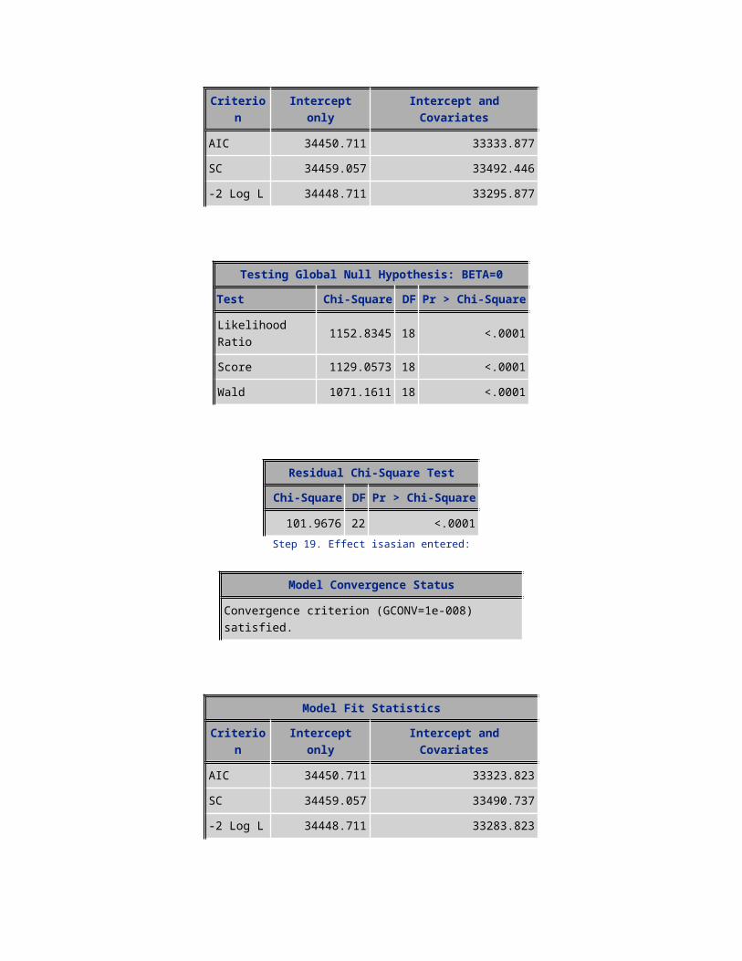
Model Fit StatisticsCriterion Intercept only Intercept and Covariates
AIC 34450.711 33333.877SC 34459.057 33492.446-2 Log L 34448.711 33295.877
Testing Global Null Hypothesis: BETA=0Test Chi-Square DF Pr > Chi-Square
Likelihood Ratio 1152.8345 18 <.0001Score 1129.0573 18 <.0001Wald 1071.1611 18 <.0001
Residual Chi-Square TestChi-Square DF Pr > Chi-Square
101.9676 22 <.0001Step 19. Effect isasian entered:
Model Convergence Status
Convergence criterion (GCONV=1e-008) satisfied.
Model Fit StatisticsCriterion Intercept only Intercept and Covariates
AIC 34450.711 33323.823SC 34459.057 33490.737-2 Log L 34448.711 33283.823
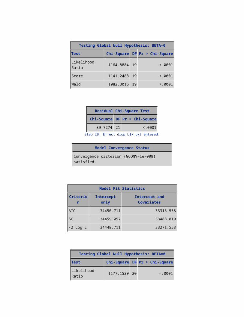
Testing Global Null Hypothesis: BETA=0Test Chi-Square DF Pr > Chi-Square
Likelihood Ratio 1164.8884 19 <.0001
Score 1141.2488 19 <.0001Wald 1082.3016 19 <.0001
Residual Chi-Square TestChi-Square DF Pr > Chi-Square
89.7274 21 <.0001Step 20. Effect drop_blk_bkt entered:
Model Convergence Status
Convergence criterion (GCONV=1e-008) satisfied.
Model Fit StatisticsCriterion Intercept only Intercept and Covariates
AIC 34450.711 33313.558SC 34459.057 33488.819-2 Log L 34448.711 33271.558
Testing Global Null Hypothesis: BETA=0Test Chi-Square DF Pr > Chi-Square
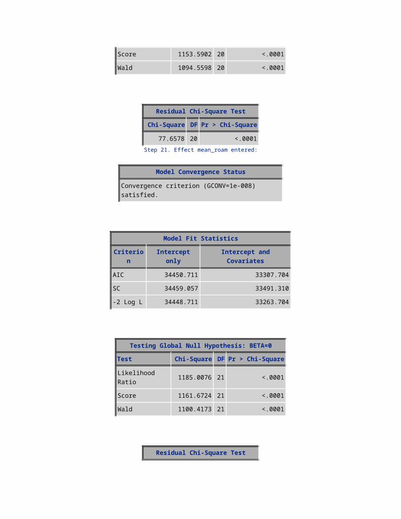
Likelihood Ratio 1177.1529 20 <.0001Score 1153.5902 20 <.0001Wald 1094.5598 20 <.0001
Residual Chi-Square TestChi-Square DF Pr > Chi-Square
77.6578 20 <.0001Step 21. Effect mean_roam entered:
Model Convergence Status
Convergence criterion (GCONV=1e-008) satisfied.

Model Fit StatisticsCriterion Intercept only Intercept and Covariates
AIC 34450.711 33307.704SC 34459.057 33491.310-2 Log L 34448.711 33263.704
Testing Global Null Hypothesis: BETA=0Test Chi-Square DF Pr > Chi-Square
Likelihood Ratio 1185.0076 21 <.0001Score 1161.6724 21 <.0001Wald 1100.4173 21 <.0001
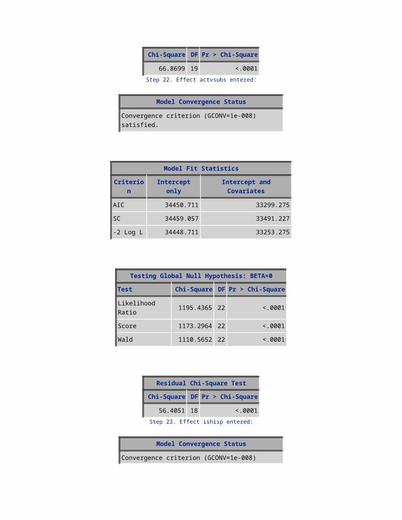
Residual Chi-Square TestChi-Square DF Pr > Chi-Square
66.8699 19 <.0001Step 22. Effect actvsubs entered:
Model Convergence Status
Convergence criterion (GCONV=1e-008) satisfied.
Model Fit StatisticsCriterion Intercept only Intercept and Covariates
AIC 34450.711 33299.275SC 34459.057 33491.227-2 Log L 34448.711 33253.275
Testing Global Null Hypothesis: BETA=0Test Chi-Square DF Pr > Chi-Square

Likelihood Ratio 1195.4365 22 <.0001Score 1173.2964 22 <.0001Wald 1110.5652 22 <.0001
Residual Chi-Square TestChi-Square DF Pr > Chi-Square
56.4051 18 <.0001Step 23. Effect ishisp entered:
Model Convergence Status
Convergence criterion (GCONV=1e-008) satisfied.
Model Fit StatisticsCriterion Intercept only Intercept and Covariates
AIC 34450.711 33293.307SC 34459.057 33493.604-2 Log L 34448.711 33245.307
Testing Global Null Hypothesis: BETA=0Test Chi-Square DF Pr > Chi-Square
Likelihood Ratio 1203.4046 23 <.0001Score 1180.8883 23 <.0001Wald 1117.5361 23 <.0001
Residual Chi-Square TestChi-Square DF Pr > Chi-Square
48.3565 17 <.0001Step 24. Effect webcap_ind entered:
Model Convergence Status
Convergence criterion (GCONV=1e-008) satisfied.
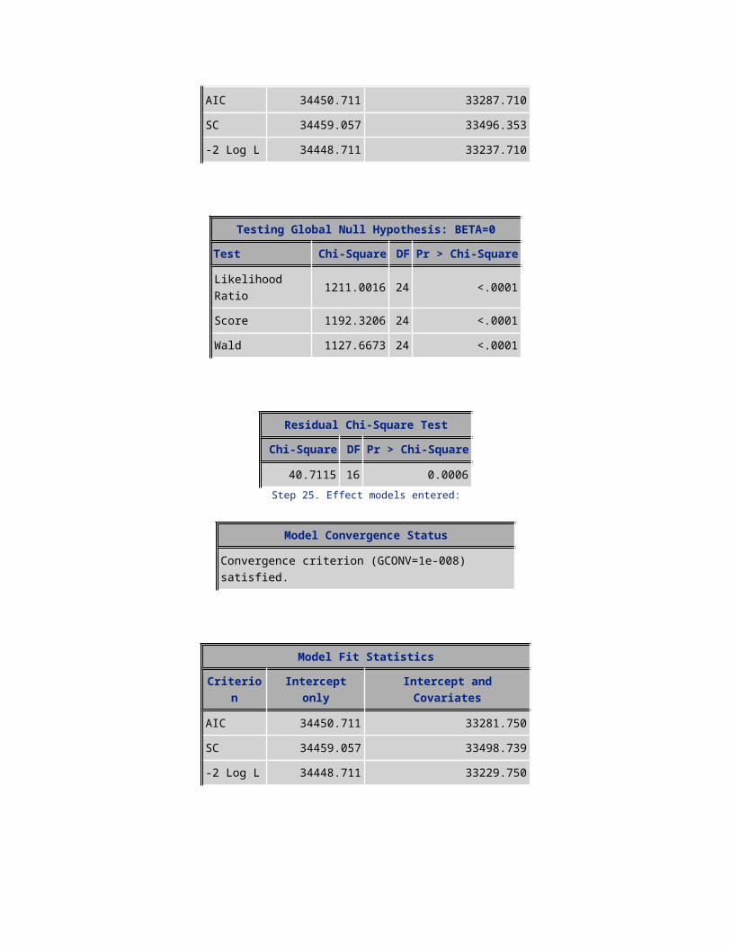
Model Fit StatisticsCriterion Intercept only Intercept and Covariates
AIC 34450.711 33287.710SC 34459.057 33496.353-2 Log L 34448.711 33237.710
Testing Global Null Hypothesis: BETA=0Test Chi-Square DF Pr > Chi-Square
Likelihood Ratio 1211.0016 24 <.0001Score 1192.3206 24 <.0001Wald 1127.6673 24 <.0001
Residual Chi-Square TestChi-Square DF Pr > Chi-Square
40.7115 16 0.0006Step 25. Effect models entered:
Model Convergence Status
Convergence criterion (GCONV=1e-008) satisfied.
Model Fit StatisticsCriterion Intercept only Intercept and Covariates
AIC 34450.711 33281.750SC 34459.057 33498.739-2 Log L 34448.711 33229.750
Testing Global Null Hypothesis: BETA=0Test Chi-Square DF Pr > Chi-Square
Likelihood Ratio 1218.9616 25 <.0001Score 1200.0611 25 <.0001Wald 1134.4058 25 <.0001
Residual Chi-Square TestChi-Square DF Pr > Chi-Square
32.6353 15 0.0053Step 26. Effect car_reg entered:
Model Convergence Status
Convergence criterion (GCONV=1e-008) satisfied.
Model Fit StatisticsCriterion Intercept only Intercept and Covariates
AIC 34450.711 33277.031SC 34459.057 33502.366-2 Log L 34448.711 33223.031
Testing Global Null Hypothesis: BETA=0Test Chi-Square DF Pr > Chi-Square
Likelihood Ratio 1225.6798 26 <.0001Score 1206.1531 26 <.0001Wald 1140.2571 26 <.0001
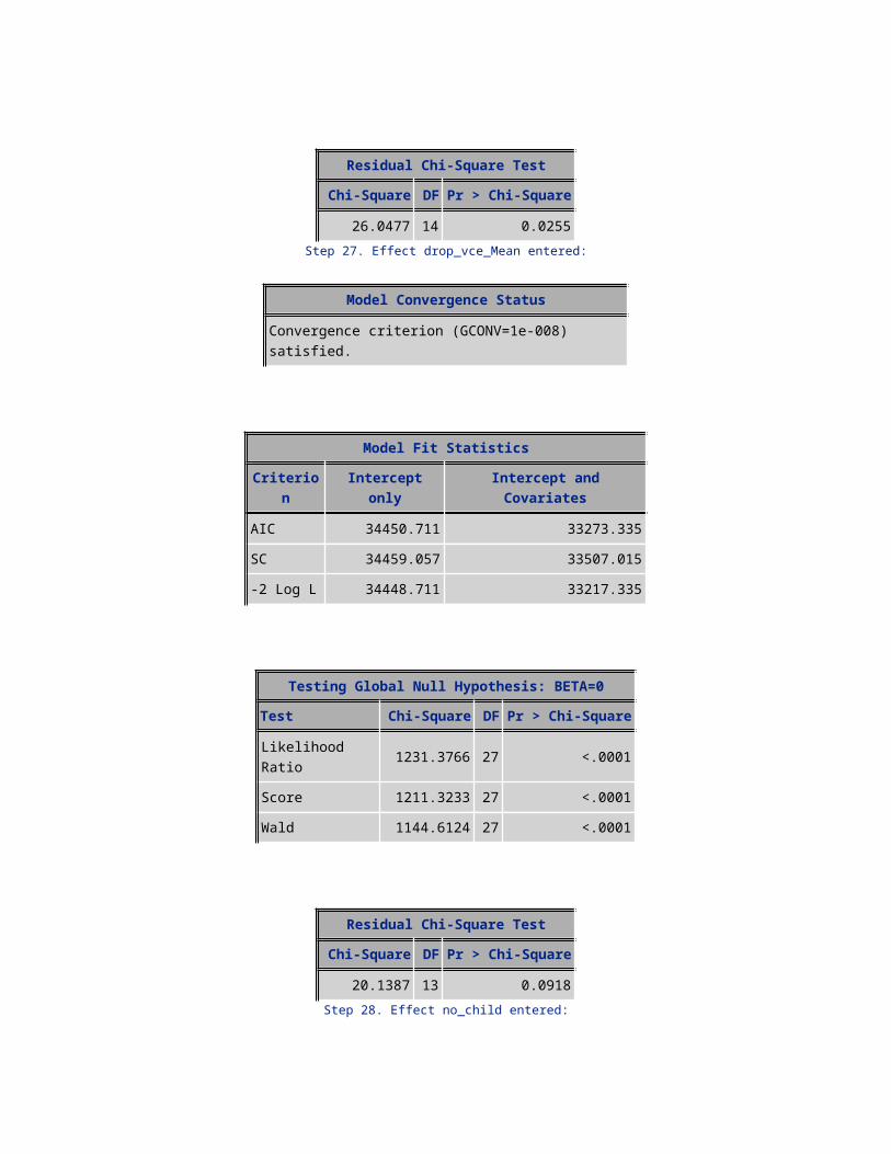
Residual Chi-Square TestChi-Square DF Pr > Chi-Square
26.0477 14 0.0255Step 27. Effect drop_vce_Mean entered:
Model Convergence Status
Convergence criterion (GCONV=1e-008) satisfied.
Model Fit StatisticsCriterion Intercept only Intercept and Covariates
AIC 34450.711 33273.335SC 34459.057 33507.015-2 Log L 34448.711 33217.335
Testing Global Null Hypothesis: BETA=0Test Chi-Square DF Pr > Chi-Square
Likelihood Ratio 1231.3766 27 <.0001Score 1211.3233 27 <.0001Wald 1144.6124 27 <.0001
Residual Chi-Square TestChi-Square DF Pr > Chi-Square
20.1387 13 0.0918Step 28. Effect no_child entered:
Model Convergence Status
Convergence criterion (GCONV=1e-008) satisfied.
Model Fit StatisticsCriterion Intercept only Intercept and Covariates
AIC 34450.711 33270.459SC 34459.057 33512.485-2 Log L 34448.711 33212.459
Testing Global Null Hypothesis: BETA=0Test Chi-Square DF Pr > Chi-Square
Likelihood Ratio 1236.2524 28 <.0001Score 1216.0508 28 <.0001Wald 1149.1918 28 <.0001
Residual Chi-Square TestChi-Square DF Pr > Chi-Square
15.3170 12 0.2246Step 29. Effect income_bkt entered:
Model Convergence Status
Convergence criterion (GCONV=1e-008) satisfied.
Model Fit StatisticsCriterion Intercept only Intercept and Covariates
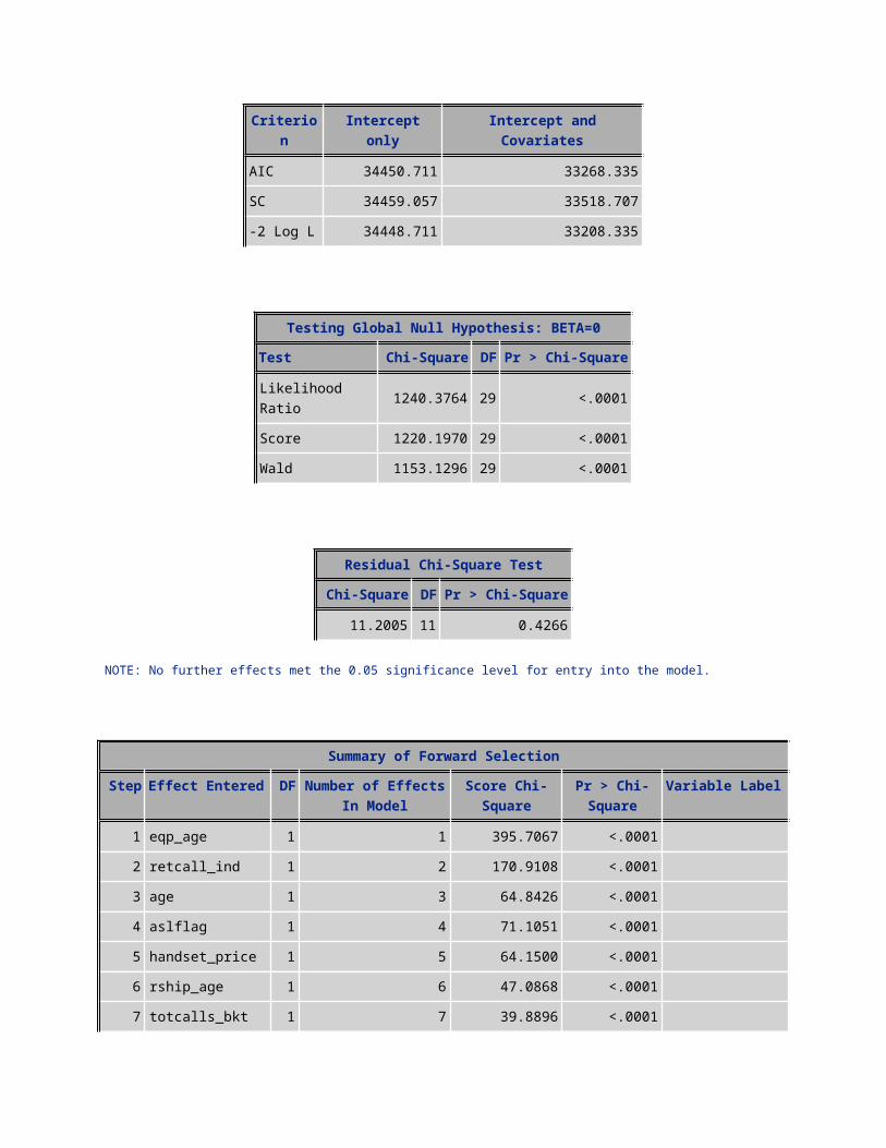
AIC 34450.711 33268.335SC 34459.057 33518.707-2 Log L 34448.711 33208.335
Testing Global Null Hypothesis: BETA=0Test Chi-Square DF Pr > Chi-Square
Likelihood Ratio 1240.3764 29 <.0001Score 1220.1970 29 <.0001Wald 1153.1296 29 <.0001
Residual Chi-Square TestChi-Square DF Pr > Chi-Square

11.2005 11 0.4266
NOTE: No further effects met the 0.05 significance level for entry into the model.
Summary of Forward Selection
Step Effect Entered DF Number of Effects In Model
Score Chi-Square
Pr > Chi-Square
Variable Label
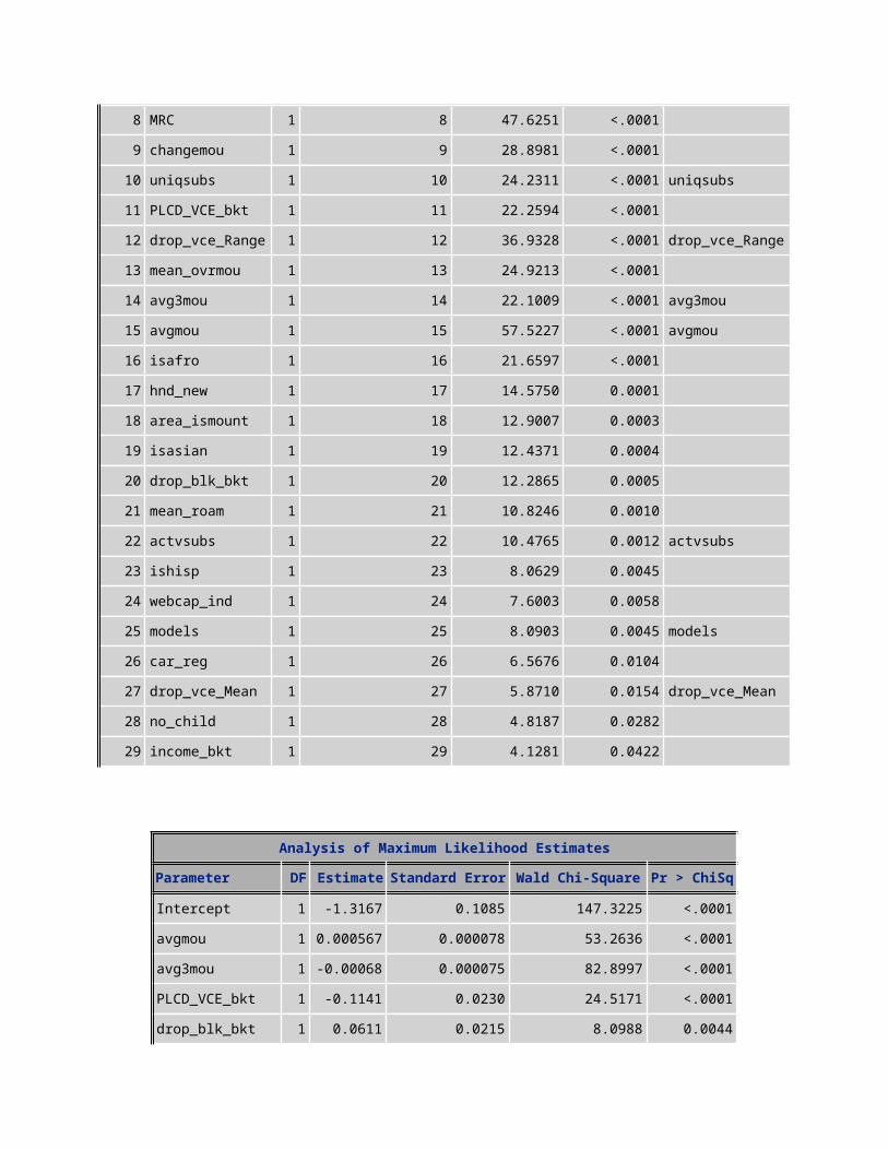
1 eqp_age 1 1 395.7067 <.0001 2 retcall_ind 1 2 170.9108 <.0001 3 age 1 3 64.8426 <.0001 4 aslflag 1 4 71.1051 <.0001 5 handset_price 1 5 64.1500 <.0001 6 rship_age 1 6 47.0868 <.0001 7 totcalls_bkt 1 7 39.8896 <.0001 8 MRC 1 8 47.6251 <.0001 9 changemou 1 9 28.8981 <.0001
10 uniqsubs 1 10 24.2311 <.0001 uniqsubs 11 PLCD_VCE_bkt 1 11 22.2594 <.0001 12 drop_vce_Range 1 12 36.9328 <.0001 drop_vce_Range13 mean_ovrmou 1 13 24.9213 <.0001 14 avg3mou 1 14 22.1009 <.0001 avg3mou 15 avgmou 1 15 57.5227 <.0001 avgmou 16 isafro 1 16 21.6597 <.0001 17 hnd_new 1 17 14.5750 0.0001 18 area_ismount 1 18 12.9007 0.0003 19 isasian 1 19 12.4371 0.0004 20 drop_blk_bkt 1 20 12.2865 0.0005 21 mean_roam 1 21 10.8246 0.0010 22 actvsubs 1 22 10.4765 0.0012 actvsubs 23 ishisp 1 23 8.0629 0.0045 24 webcap_ind 1 24 7.6003 0.0058 25 models 1 25 8.0903 0.0045 models 26 car_reg 1 26 6.5676 0.0104 27 drop_vce_Mean 1 27 5.8710 0.0154 drop_vce_Mean
28 no_child 1 28 4.8187 0.0282 29 income_bkt 1 29 4.1281 0.0422
Analysis of Maximum Likelihood EstimatesParameter DF Estimate Standard Error Wald Chi-Square Pr > ChiSq
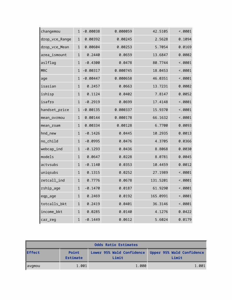
Intercept 1 -1.3167 0.1085 147.3225 <.0001avgmou 1 0.000567 0.000078 53.2636 <.0001avg3mou 1 -0.00068 0.000075 82.8997 <.0001PLCD_VCE_bkt 1 -0.1141 0.0230 24.5171 <.0001drop_blk_bkt 1 0.0611 0.0215 8.0988 0.0044changemou 1 -0.00038 0.000059 42.5105 <.0001drop_vce_Range 1 0.00392 0.00245 2.5628 0.1094drop_vce_Mean 1 0.00604 0.00253 5.7054 0.0169area_ismount 1 0.2440 0.0659 13.6847 0.0002aslflag 1 -0.4300 0.0478 80.7744 <.0001MRC 1 -0.00317 0.000745 18.0453 <.0001age 1 -0.00447 0.000658 46.0351 <.0001isasian 1 0.2457 0.0663 13.7231 0.0002ishisp 1 0.1124 0.0402 7.8147 0.0052isafro 1 -0.2919 0.0699 17.4148 <.0001handset_price 1 -0.00135 0.000337 15.9370 <.0001mean_ovrmou 1 0.00144 0.000178 66.1632 <.0001mean_roam 1 0.00334 0.00128 6.7700 0.0093hnd_new 1 -0.1426 0.0445 10.2935 0.0013no_child 1 -0.0995 0.0476 4.3705 0.0366webcap_ind 1 -0.1293 0.0436 8.8068 0.0030models 1 0.0647 0.0228 8.0781 0.0045actvsubs 1 -0.1140 0.0353 10.4459 0.0012uniqsubs 1 0.1315 0.0252 27.1989 <.0001retcall_ind 1 0.7776 0.0678 131.5201 <.0001rship_age 1 -0.1470 0.0187 61.9290 <.0001eqp_age 1 0.2469 0.0192 165.0991 <.0001totcalls_bkt 1 0.2419 0.0401 36.3146 <.0001

income_bkt 1 0.0285 0.0140 4.1276 0.0422car_reg 1 -0.1449 0.0612 5.6024 0.0179
Odds Ratio EstimatesEffect Point
EstimateLower 95% Wald Confidence
LimitUpper 95% Wald Confidence Limit
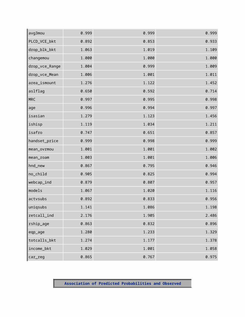
avgmou 1.001 1.000 1.001avg3mou 0.999 0.999 0.999PLCD_VCE_bkt 0.892 0.853 0.933drop_blk_bkt 1.063 1.019 1.109changemou 1.000 1.000 1.000drop_vce_Range 1.004 0.999 1.009drop_vce_Mean 1.006 1.001 1.011area_ismount 1.276 1.122 1.452aslflag 0.650 0.592 0.714MRC 0.997 0.995 0.998age 0.996 0.994 0.997isasian 1.279 1.123 1.456ishisp 1.119 1.034 1.211isafro 0.747 0.651 0.857handset_price 0.999 0.998 0.999mean_ovrmou 1.001 1.001 1.002mean_roam 1.003 1.001 1.006hnd_new 0.867 0.795 0.946no_child 0.905 0.825 0.994webcap_ind 0.879 0.807 0.957models 1.067 1.020 1.116actvsubs 0.892 0.833 0.956uniqsubs 1.141 1.086 1.198retcall_ind 2.176 1.905 2.486rship_age 0.863 0.832 0.896eqp_age 1.280 1.233 1.329totcalls_bkt 1.274 1.177 1.378
income_bkt 1.029 1.001 1.058car_reg 0.865 0.767 0.975
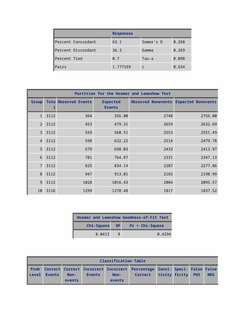
Association of Predicted Probabilities and Observed Responses
Percent Concordant 63.1 Somer's D 0.268Percent Discordant 36.3 Gamma 0.269Percent Tied 0.7 Tau-a 0.098Pairs 1.7771E8 c 0.634
Partition for the Hosmer and Lemeshow TestGroup Total Observed
EventsExpected Events
Observed Nonevents
Expected Nonevents
1 3112 364 356.00 2748 2756.002 3112 453 479.31 2659 2632.693 3112 559 560.51 2553 2551.494 3112 598 632.22 2514 2479.785 3112 679 698.03 2433 2413.976 3112 781 764.87 2331 2347.137 3112 825 834.14 2287 2277.868 3112 947 913.01 2165 2198.999 3112 1028 1016.43 2084 2095.57
10 3116 1299 1278.48 1817 1837.52
Hosmer and Lemeshow Goodness-of-Fit TestChi-Square DF Pr > Chi-Square
8.0413 8 0.4294
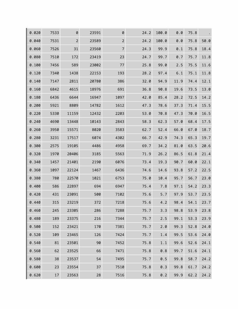
Classification Table

Prob Level
Correct Events
Correct Non-
events
Incorrect Events
Incorrect Non-
events
Percentage Correct
Sensi- tivity
Speci- ficity
False POS
False NEG
0.020 7533 0 23591 0 24.2 100.0 0.0 75.8 . 0.040 7531 2 23589 2 24.2 100.0 0.0 75.8 50.00.060 7526 31 23560 7 24.3 99.9 0.1 75.8 18.40.080 7510 172 23419 23 24.7 99.7 0.7 75.7 11.80.100 7456 589 23002 77 25.8 99.0 2.5 75.5 11.60.120 7340 1438 22153 193 28.2 97.4 6.1 75.1 11.80.140 7147 2811 20780 386 32.0 94.9 11.9 74.4 12.10.160 6842 4615 18976 691 36.8 90.8 19.6 73.5 13.00.180 6436 6644 16947 1097 42.0 85.4 28.2 72.5 14.20.200 5921 8809 14782 1612 47.3 78.6 37.3 71.4 15.50.220 5330 11159 12432 2203 53.0 70.8 47.3 70.0 16.50.240 4690 13448 10143 2843 58.3 62.3 57.0 68.4 17.50.260 3950 15571 8020 3583 62.7 52.4 66.0 67.0 18.70.280 3231 17517 6074 4302 66.7 42.9 74.3 65.3 19.70.300 2575 19105 4486 4958 69.7 34.2 81.0 63.5 20.60.320 1970 20406 3185 5563 71.9 26.2 86.5 61.8 21.40.340 1457 21401 2190 6076 73.4 19.3 90.7 60.0 22.10.360 1097 22124 1467 6436 74.6 14.6 93.8 57.2 22.50.380 780 22570 1021 6753 75.0 10.4 95.7 56.7 23.00.400 586 22897 694 6947 75.4 7.8 97.1 54.2 23.30.420 431 23091 500 7102 75.6 5.7 97.9 53.7 23.50.440 315 23219 372 7218 75.6 4.2 98.4 54.1 23.70.460 245 23305 286 7288 75.7 3.3 98.8 53.9 23.80.480 189 23375 216 7344 75.7 2.5 99.1 53.3 23.90.500 152 23421 170 7381 75.7 2.0 99.3 52.8 24.00.520 109 23465 126 7424 75.7 1.4 99.5 53.6 24.00.540 81 23501 90 7452 75.8 1.1 99.6 52.6 24.10.560 62 23525 66 7471 75.8 0.8 99.7 51.6 24.10.580 38 23537 54 7495 75.7 0.5 99.8 58.7 24.20.600 23 23554 37 7510 75.8 0.3 99.8 61.7 24.20.620 17 23563 28 7516 75.8 0.2 99.9 62.2 24.20.640 8 23571 20 7525 75.8 0.1 99.9 71.4 24.2
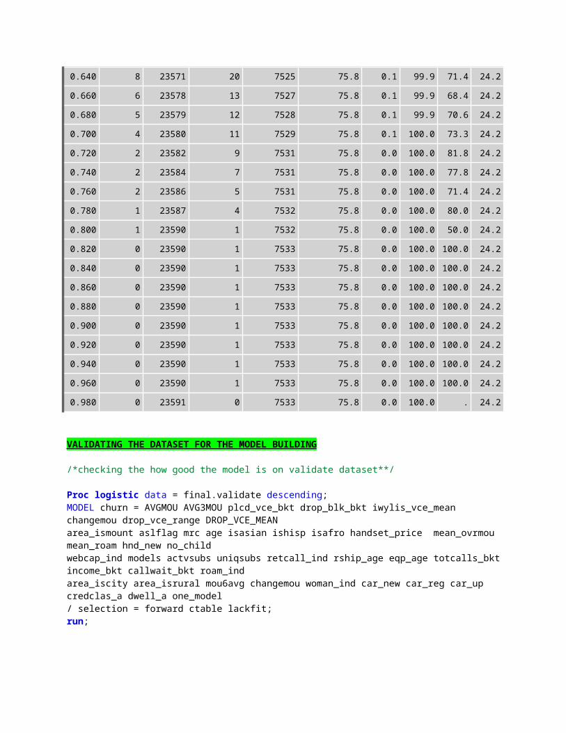
0.660 6 23578 13 7527 75.8 0.1 99.9 68.4 24.20.680 5 23579 12 7528 75.8 0.1 99.9 70.6 24.20.700 4 23580 11 7529 75.8 0.1 100.0 73.3 24.20.720 2 23582 9 7531 75.8 0.0 100.0 81.8 24.20.740 2 23584 7 7531 75.8 0.0 100.0 77.8 24.20.760 2 23586 5 7531 75.8 0.0 100.0 71.4 24.20.780 1 23587 4 7532 75.8 0.0 100.0 80.0 24.20.800 1 23590 1 7532 75.8 0.0 100.0 50.0 24.20.820 0 23590 1 7533 75.8 0.0 100.0 100.0 24.20.840 0 23590 1 7533 75.8 0.0 100.0 100.0 24.20.860 0 23590 1 7533 75.8 0.0 100.0 100.0 24.20.880 0 23590 1 7533 75.8 0.0 100.0 100.0 24.20.900 0 23590 1 7533 75.8 0.0 100.0 100.0 24.20.920 0 23590 1 7533 75.8 0.0 100.0 100.0 24.20.940 0 23590 1 7533 75.8 0.0 100.0 100.0 24.20.960 0 23590 1 7533 75.8 0.0 100.0 100.0 24.20.980 0 23591 0 7533 75.8 0.0 100.0 . 24.2
VALIDATING THE DATASET FOR THE MODEL BUILDING
/*checking the how good the model is on validate dataset**/
Proc logistic data = final.validate descending;MODEL churn = AVGMOU AVG3MOU plcd_vce_bkt drop_blk_bkt iwylis_vce_mean changemou drop_vce_range DROP_VCE_MEAN area_ismount aslflag mrc age isasian ishisp isafro handset_price mean_ovrmou mean_roam hnd_new no_child webcap_ind models actvsubs uniqsubs retcall_ind rship_age eqp_age totcalls_bkt income_bkt callwait_bkt roam_ind area_iscity area_isrural mou6avg changemou woman_ind car_new car_reg car_up credclas_a dwell_a one_model / selection = forward ctable lackfit;run;
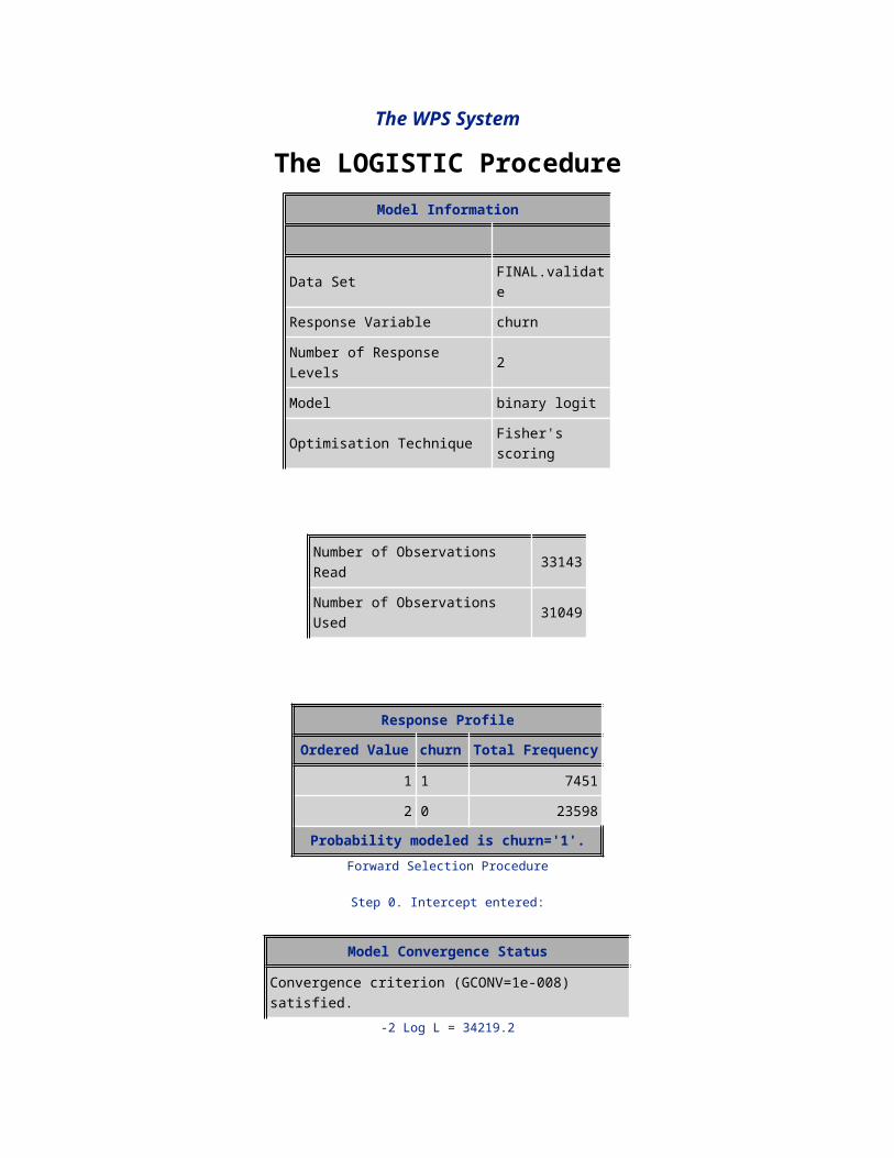
The WPS System
The LOGISTIC ProcedureModel Information
Data Set FINAL.validateResponse Variable churnNumber of Response Levels 2Model binary logitOptimisation Technique Fisher's scoring
Number of Observations Read 33143Number of Observations Used 31049
Response ProfileOrdered Value churn Total
Frequency
1 1 74512 0 23598
Probability modeled is churn='1'.Forward Selection Procedure
Step 0. Intercept entered:
Model Convergence Status
Convergence criterion (GCONV=1e-008) satisfied.-2 Log L = 34219.2
Residual Chi-Square Test
Chi-Square DF Pr > Chi-Square
1177.5278 40 <.0001Step 1. Effect eqp_age entered:
Model Convergence Status
Convergence criterion (GCONV=1e-008) satisfied.
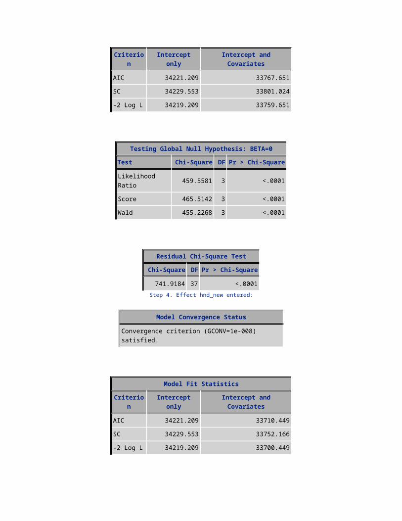
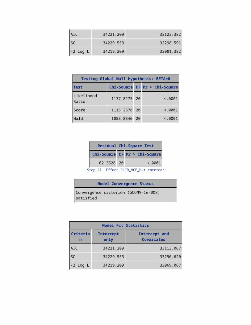
Model Fit Statistics
Criterion Intercept only Intercept and Covariates
AIC 34221.209 33920.358SC 34229.553 33937.045-2 Log L 34219.209 33916.358
Testing Global Null Hypothesis: BETA=0Test Chi-Square DF Pr > Chi-Square
Likelihood Ratio 302.8509 1 <.0001Score 300.8859 1 <.0001Wald 298.2020 1 <.0001
Residual Chi-Square TestChi-Square DF Pr > Chi-Square
910.4723 39 <.0001Step 2. Effect retcall_ind entered:
Model Convergence Status
Convergence criterion (GCONV=1e-008) satisfied.
Model Fit StatisticsCriterion Intercept only Intercept and Covariates
AIC 34221.209 33831.040SC 34229.553 33856.070-2 Log L 34219.209 33825.040
Testing Global Null Hypothesis: BETA=0Test Chi-Square DF Pr > Chi-Square
Likelihood Ratio 394.1691 2 <.0001Score 399.1679 2 <.0001
Wald 391.3533 2 <.0001
Residual Chi-Square TestChi-Square DF Pr > Chi-Square
810.8576 38 <.0001Step 3. Effect uniqsubs entered:
Model Convergence Status
Convergence criterion (GCONV=1e-008) satisfied.
Model Fit StatisticsCriterion Intercept only Intercept and Covariates
AIC 34221.209 33767.651SC 34229.553 33801.024-2 Log L 34219.209 33759.651
Testing Global Null Hypothesis: BETA=0Test Chi-Square DF Pr > Chi-Square
Likelihood Ratio 459.5581 3 <.0001Score 465.5142 3 <.0001Wald 455.2268 3 <.0001
Residual Chi-Square TestChi-Square DF Pr > Chi-Square
741.9184 37 <.0001Step 4. Effect hnd_new entered:
Model Convergence Status
Convergence criterion (GCONV=1e-008) satisfied.
Model Fit StatisticsCriterion Intercept only Intercept and Covariates
AIC 34221.209 33710.449SC 34229.553 33752.166-2 Log L 34219.209 33700.449
Testing Global Null Hypothesis: BETA=0Test Chi-Square DF Pr > Chi-Square
Likelihood Ratio 518.7601 4 <.0001Score 524.4062 4 <.0001Wald 512.1788 4 <.0001
Residual Chi-Square TestChi-Square DF Pr > Chi-Square
682.1505 36 <.0001Step 5. Effect age entered:
Model Convergence Status
Convergence criterion (GCONV=1e-008) satisfied.
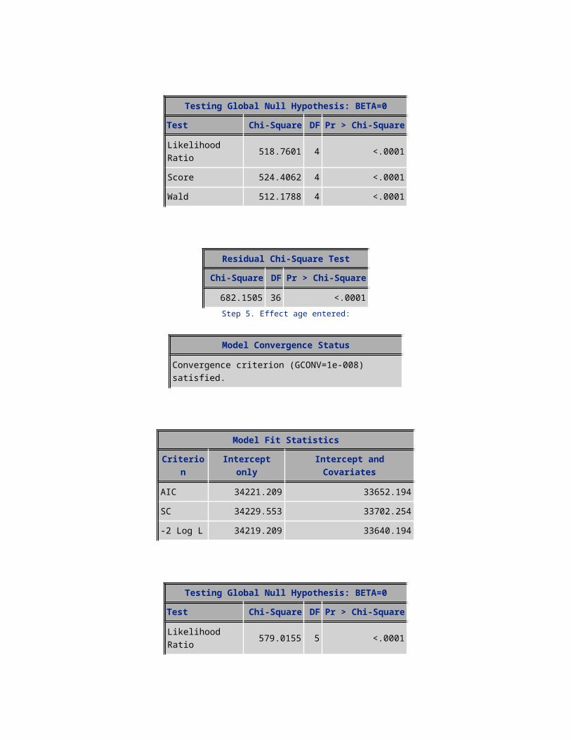
Model Fit StatisticsCriterion Intercept only Intercept and Covariates
AIC 34221.209 33652.194SC 34229.553 33702.254-2 Log L 34219.209 33640.194
Testing Global Null Hypothesis: BETA=0Test Chi-Square DF Pr > Chi-Square
Likelihood Ratio 579.0155 5 <.0001Score 583.4429 5 <.0001Wald 568.6121 5 <.0001
Residual Chi-Square TestChi-Square DF Pr > Chi-Square
620.2075 35 <.0001Step 6. Effect isafro entered:
Model Convergence Status
Convergence criterion (GCONV=1e-008) satisfied.
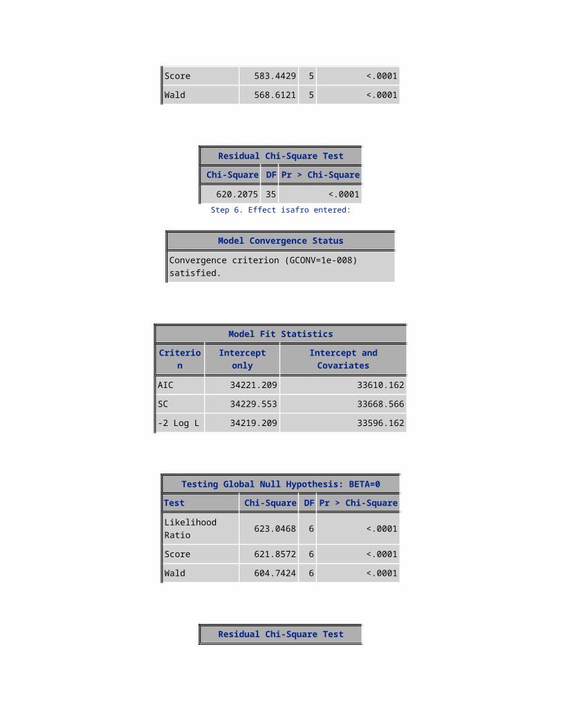
Model Fit StatisticsCriterion Intercept only Intercept and Covariates
AIC 34221.209 33610.162SC 34229.553 33668.566-2 Log L 34219.209 33596.162
Testing Global Null Hypothesis: BETA=0Test Chi-Square DF Pr > Chi-Square
Likelihood Ratio 623.0468 6 <.0001Score 621.8572 6 <.0001Wald 604.7424 6 <.0001
Residual Chi-Square TestChi-Square DF Pr > Chi-Square
580.9746 34 <.0001Step 7. Effect MRC entered:
Model Convergence Status
Convergence criterion (GCONV=1e-008) satisfied.
Model Fit StatisticsCriterion Intercept only Intercept and Covariates
AIC 34221.209 33571.264SC 34229.553 33638.010-2 Log L 34219.209 33555.264
Testing Global Null Hypothesis: BETA=0Test Chi-Square DF Pr > Chi-Square
Likelihood Ratio 663.9455 7 <.0001Score 660.2436 7 <.0001Wald 641.6473 7 <.0001
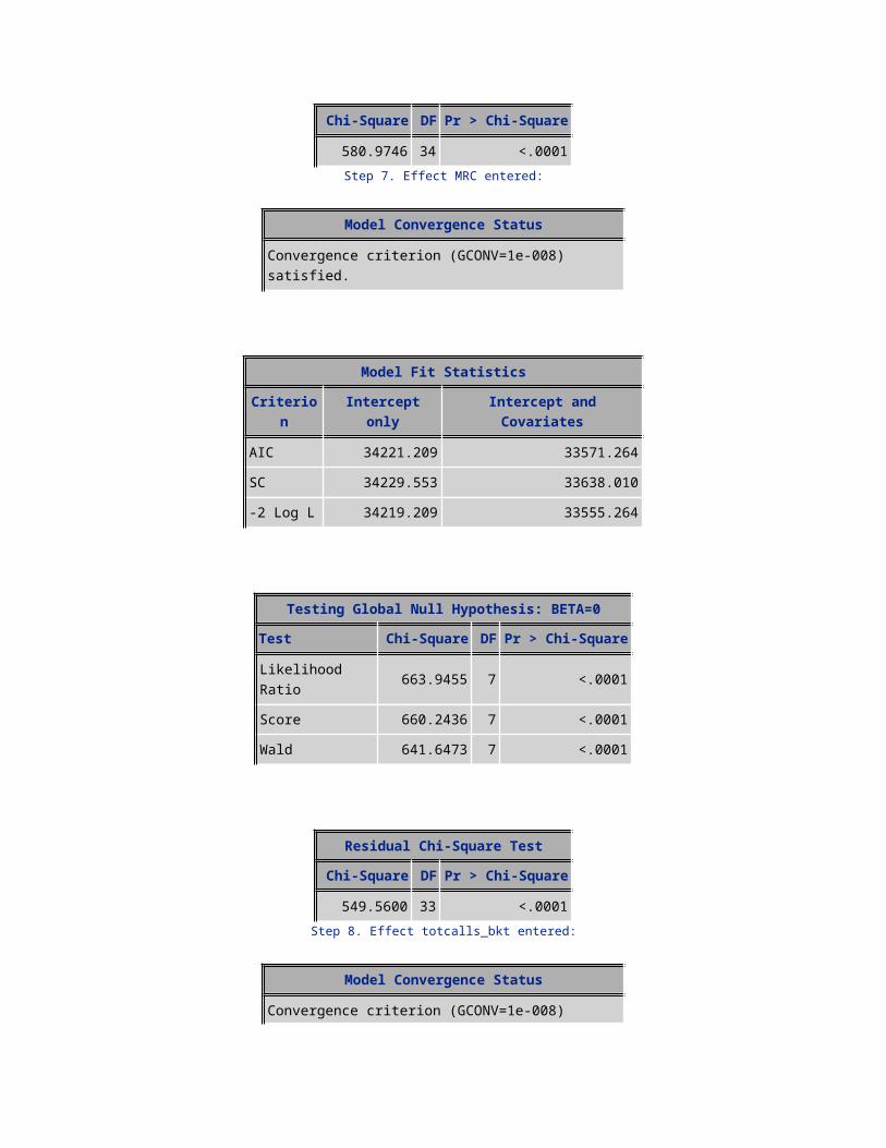
Residual Chi-Square TestChi-Square DF Pr > Chi-Square
549.5600 33 <.0001Step 8. Effect totcalls_bkt entered:
Model Convergence Status
Convergence criterion (GCONV=1e-008) satisfied.
Model Fit StatisticsCriterion Intercept only Intercept and Covariates
AIC 34221.209 33521.110SC 34229.553 33596.200-2 Log L 34219.209 33503.110
Testing Global Null Hypothesis: BETA=0Test Chi-Square DF Pr > Chi-Square
Likelihood Ratio 716.0991 8 <.0001Score 712.0775 8 <.0001Wald 691.3940 8 <.0001
Residual Chi-Square TestChi-Square DF Pr > Chi-Square
488.3136 32 <.0001Step 9. Effect rship_age entered:
Model Convergence Status
Convergence criterion (GCONV=1e-008) satisfied.
Model Fit StatisticsCriterion Intercept only Intercept and Covariates
AIC 34221.209 33482.650SC 34229.553 33566.084-2 Log L 34219.209 33462.650
Testing Global Null Hypothesis: BETA=0Test Chi-Square DF Pr > Chi-Square
Likelihood Ratio 756.5589 9 <.0001Score 745.7204 9 <.0001Wald 722.2831 9 <.0001
Residual Chi-Square TestChi-Square DF Pr > Chi-Square
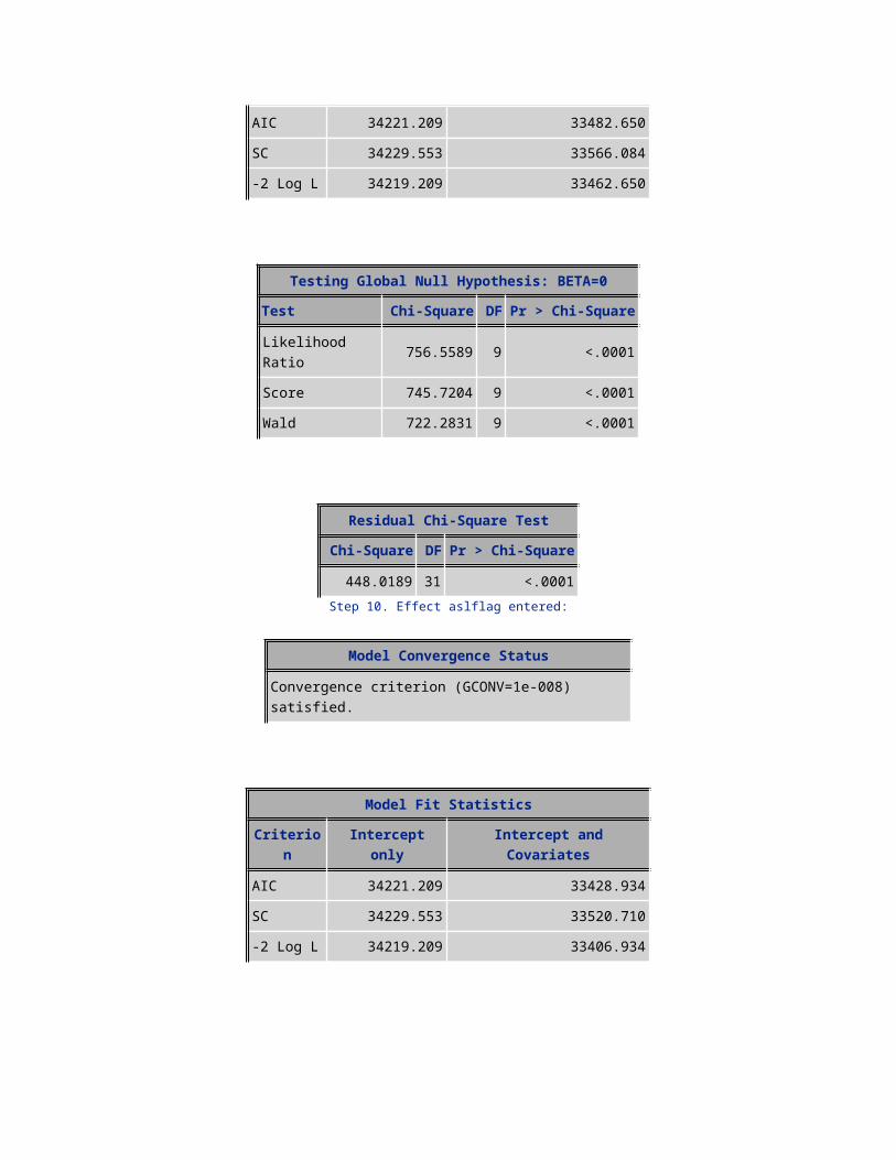
448.0189 31 <.0001Step 10. Effect aslflag entered:

Model Convergence Status
Convergence criterion (GCONV=1e-008) satisfied.
Model Fit StatisticsCriterion Intercept only Intercept and Covariates
AIC 34221.209 33428.934SC 34229.553 33520.710-2 Log L 34219.209 33406.934
Testing Global Null Hypothesis: BETA=0Test Chi-Square DF Pr > Chi-Square
Likelihood Ratio 812.2756 10 <.0001Score 795.7781 10 <.0001Wald 770.1978 10 <.0001
Residual Chi-Square TestChi-Square DF Pr > Chi-Square
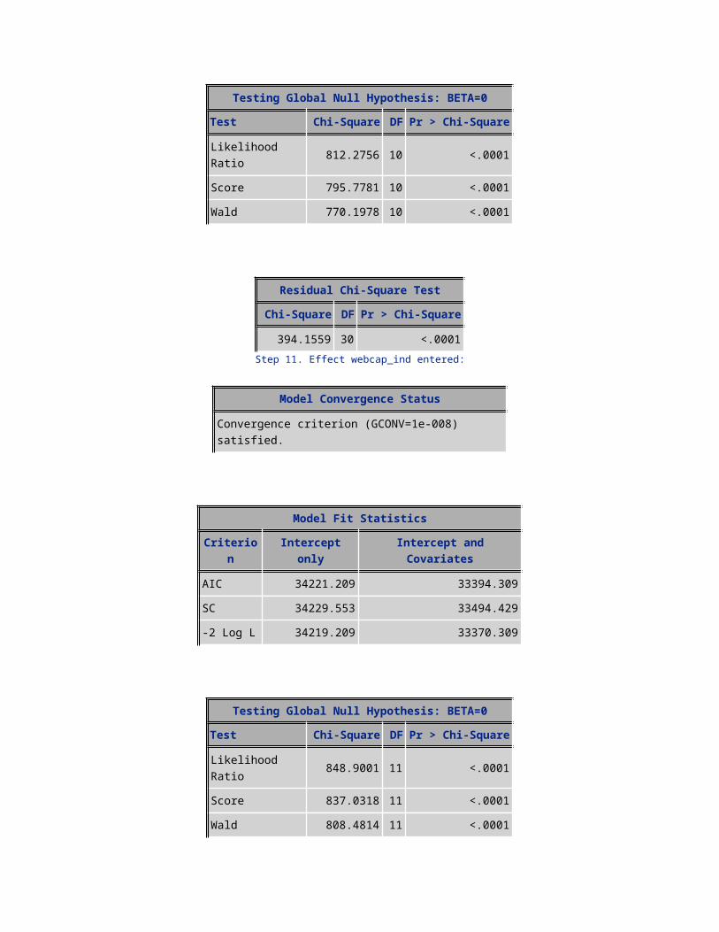
394.1559 30 <.0001Step 11. Effect webcap_ind entered:
Model Convergence Status
Convergence criterion (GCONV=1e-008) satisfied.
Model Fit StatisticsCriterion Intercept only Intercept and Covariates
AIC 34221.209 33394.309SC 34229.553 33494.429-2 Log L 34219.209 33370.309

Testing Global Null Hypothesis: BETA=0Test Chi-Square DF Pr > Chi-Square
Likelihood Ratio 848.9001 11 <.0001Score 837.0318 11 <.0001Wald 808.4814 11 <.0001
Residual Chi-Square TestChi-Square DF Pr > Chi-Square
357.0971 29 <.0001Step 12. Effect isasian entered:
Model Convergence Status
Convergence criterion (GCONV=1e-008) satisfied.
Model Fit StatisticsCriterion Intercept only Intercept and Covariates
AIC 34221.209 33364.242SC 34229.553 33472.705-2 Log L 34219.209 33338.242
Testing Global Null Hypothesis: BETA=0Test Chi-Square DF Pr > Chi-Square
Likelihood Ratio 880.9674 12 <.0001Score 871.6385 12 <.0001Wald 840.3767 12 <.0001
Residual Chi-Square TestChi-Square DF Pr > Chi-Square
323.6032 28 <.0001Step 13. Effect mean_ovrmou entered:
Model Convergence Status
Convergence criterion (GCONV=1e-008) satisfied.
Model Fit StatisticsCriterion Intercept only Intercept and Covariates
AIC 34221.209 33339.703SC 34229.553 33456.510-2 Log L 34219.209 33311.703
Testing Global Null Hypothesis: BETA=0Test Chi-Square DF Pr > Chi-Square
Likelihood Ratio 907.5062 13 <.0001Score 898.1250 13 <.0001Wald 863.6643 13 <.0001
Residual Chi-Square TestChi-Square DF Pr > Chi-Square
291.9235 27 <.0001Step 14. Effect avg3mou entered:
Model Convergence Status
Convergence criterion (GCONV=1e-008) satisfied.
Model Fit StatisticsCriterion Intercept only Intercept and Covariates
AIC 34221.209 33291.647SC 34229.553 33416.797
-2 Log L 34219.209 33261.647
Testing Global Null Hypothesis: BETA=0Test Chi-Square DF Pr > Chi-Square
Likelihood Ratio 957.5622 14 <.0001Score 945.0097 14 <.0001Wald 905.9672 14 <.0001
Residual Chi-Square TestChi-Square DF Pr > Chi-Square
249.6822 26 <.0001Step 15. Effect avgmou entered:
Model Convergence Status
Convergence criterion (GCONV=1e-008) satisfied.
Model Fit StatisticsCriterion Intercept only Intercept and Covariates
AIC 34221.209 33225.748SC 34229.553 33359.241-2 Log L 34219.209 33193.748
Testing Global Null Hypothesis: BETA=0Test Chi-Square DF Pr > Chi-Square
Likelihood Ratio 1025.4613 15 <.0001Score 1006.0867 15 <.0001Wald 960.8460 15 <.0001
Residual Chi-Square TestChi-Square DF Pr > Chi-Square
181.8526 25 <.0001Step 16. Effect drop_vce_Range entered:
Model Convergence Status
Convergence criterion (GCONV=1e-008) satisfied.
Model Fit StatisticsCriterion Intercept only Intercept and Covariates
AIC 34221.209 33202.698SC 34229.553 33344.535-2 Log L 34219.209 33168.698
Testing Global Null Hypothesis: BETA=0Test Chi-Square DF Pr > Chi-Square
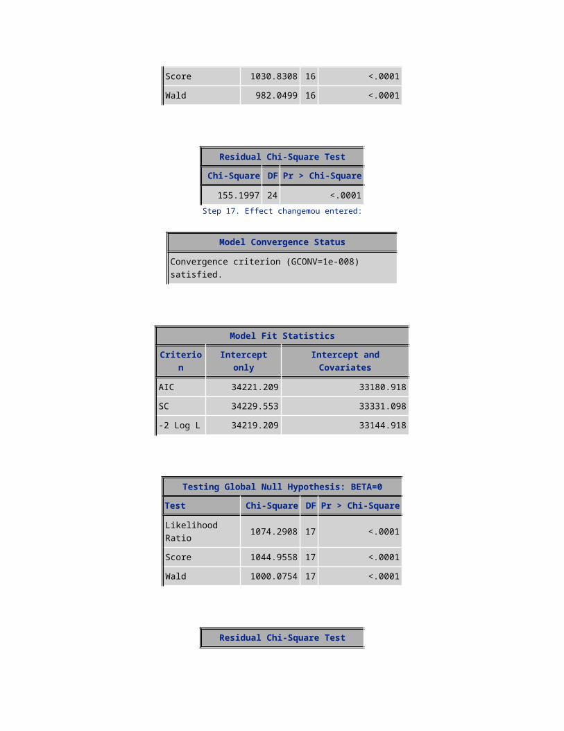
Likelihood Ratio 1050.5109 16 <.0001Score 1030.8308 16 <.0001Wald 982.0499 16 <.0001
Residual Chi-Square TestChi-Square DF Pr > Chi-Square
155.1997 24 <.0001Step 17. Effect changemou entered:
Model Convergence Status
Convergence criterion (GCONV=1e-008) satisfied.
Model Fit StatisticsCriterion Intercept only Intercept and Covariates
AIC 34221.209 33180.918SC 34229.553 33331.098-2 Log L 34219.209 33144.918
Testing Global Null Hypothesis: BETA=0Test Chi-Square DF Pr > Chi-Square
Likelihood Ratio 1074.2908 17 <.0001Score 1044.9558 17 <.0001Wald 1000.0754 17 <.0001
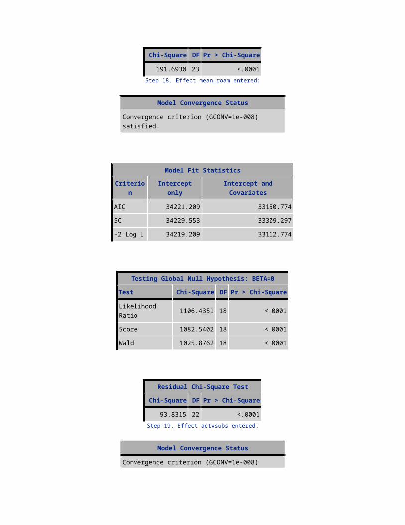
Residual Chi-Square TestChi-Square DF Pr > Chi-Square
191.6930 23 <.0001Step 18. Effect mean_roam entered:
Model Convergence Status
Convergence criterion (GCONV=1e-008) satisfied.
Model Fit StatisticsCriterion Intercept only Intercept and Covariates
AIC 34221.209 33150.774SC 34229.553 33309.297-2 Log L 34219.209 33112.774
Testing Global Null Hypothesis: BETA=0Test Chi-Square DF Pr > Chi-Square
Likelihood Ratio 1106.4351 18 <.0001Score 1082.5402 18 <.0001Wald 1025.8762 18 <.0001

Residual Chi-Square TestChi-Square DF Pr > Chi-Square
93.8315 22 <.0001Step 19. Effect actvsubs entered:
Model Convergence Status
Convergence criterion (GCONV=1e-008) satisfied.
Model Fit StatisticsCriterion Intercept only Intercept and Covariates
AIC 34221.209 33134.679SC 34229.553 33301.545-2 Log L 34219.209 33094.679
Testing Global Null Hypothesis: BETA=0Test Chi-Square DF Pr > Chi-Square
Likelihood Ratio 1124.5304 19 <.0001Score 1102.7041 19 <.0001Wald 1042.4785 19 <.0001
Residual Chi-Square TestChi-Square DF Pr > Chi-Square
75.7138 21 <.0001Step 20. Effect one_model entered:
Model Convergence Status
Convergence criterion (GCONV=1e-008) satisfied.
Model Fit StatisticsCriterion Intercept only Intercept and Covariates
AIC 34221.209 33123.382SC 34229.553 33298.591-2 Log L 34219.209 33081.382
Testing Global Null Hypothesis: BETA=0Test Chi-Square DF Pr > Chi-Square
Likelihood Ratio 1137.8275 20 <.0001Score 1115.2578 20 <.0001Wald 1053.8346 20 <.0001
Residual Chi-Square TestChi-Square DF Pr > Chi-Square
62.3528 20 <.0001Step 21. Effect PLCD_VCE_bkt entered:
Model Convergence Status
Convergence criterion (GCONV=1e-008) satisfied.
Model Fit StatisticsCriterion Intercept only Intercept and Covariates
AIC 34221.209 33113.067SC 34229.553 33296.620-2 Log L 34219.209 33069.067
Testing Global Null Hypothesis: BETA=0Test Chi-Square DF Pr > Chi-Square
Likelihood Ratio 1150.1426 21 <.0001
Score 1131.0524 21 <.0001Wald 1066.8021 21 <.0001
Residual Chi-Square TestChi-Square DF Pr > Chi-Square
50.0641 19 0.0001Step 22. Effect drop_blk_bkt entered:
Model Convergence Status
Convergence criterion (GCONV=1e-008) satisfied.
Model Fit StatisticsCriterion Intercept only Intercept and Covariates
AIC 34221.209 33102.376SC 34229.553 33294.273-2 Log L 34219.209 33056.376
Testing Global Null Hypothesis: BETA=0Test Chi-Square DF Pr > Chi-Square
Likelihood Ratio 1162.8329 22 <.0001Score 1143.5578 22 <.0001Wald 1079.6047 22 <.0001
Residual Chi-Square TestChi-Square DF Pr > Chi-Square
37.4052 18 0.0046Step 23. Effect area_ismount entered:
Model Convergence Status
Convergence criterion (GCONV=1e-008) satisfied.

Model Fit StatisticsCriterion Intercept only Intercept and Covariates
AIC 34221.209 33094.139SC 34229.553 33294.378-2 Log L 34219.209 33046.139
Testing Global Null Hypothesis: BETA=0Test Chi-Square DF Pr > Chi-Square
Likelihood Ratio 1173.0707 23 <.0001Score 1153.7958 23 <.0001Wald 1089.2678 23 <.0001
Residual Chi-Square TestChi-Square DF Pr > Chi-Square
26.8637 17 0.0601Step 24. Effect handset_price entered:
Model Convergence Status
Convergence criterion (GCONV=1e-008) satisfied.
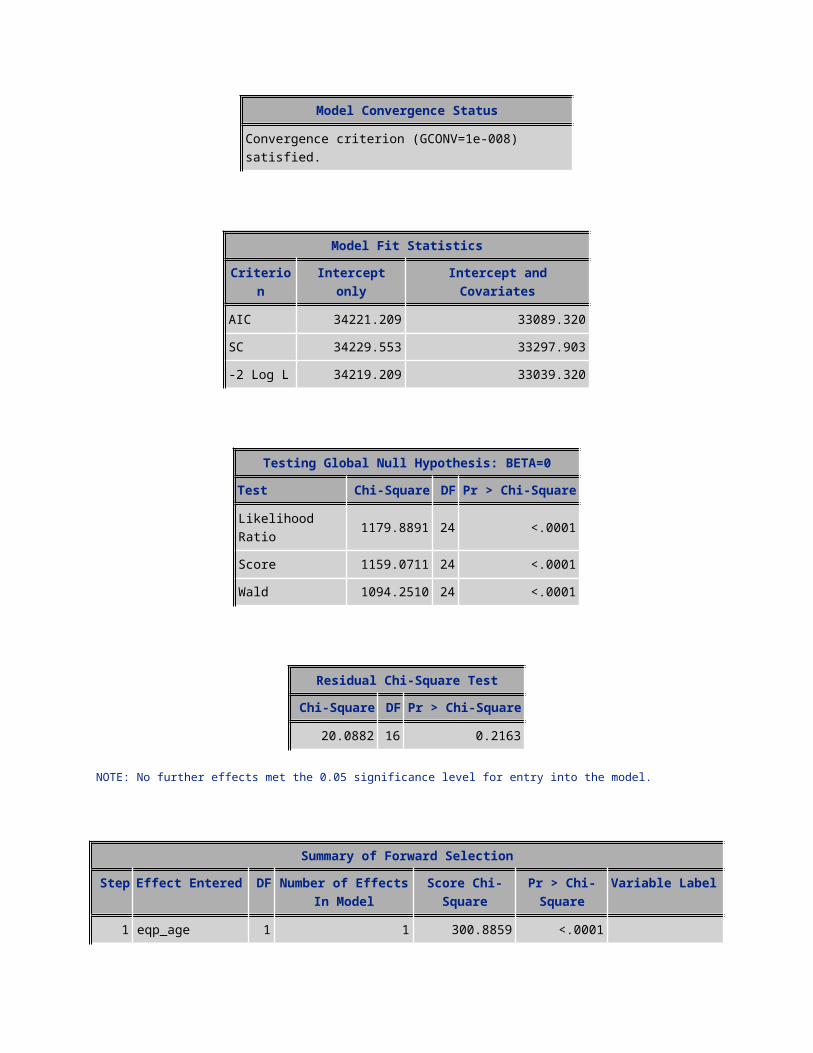
Model Fit StatisticsCriterion Intercept only Intercept and Covariates
AIC 34221.209 33089.320SC 34229.553 33297.903-2 Log L 34219.209 33039.320
Testing Global Null Hypothesis: BETA=0Test Chi-Square DF Pr > Chi-Square

Likelihood Ratio 1179.8891 24 <.0001Score 1159.0711 24 <.0001Wald 1094.2510 24 <.0001
Residual Chi-Square TestChi-Square DF Pr > Chi-Square
20.0882 16 0.2163
NOTE: No further effects met the 0.05 significance level for entry into the model.
Summary of Forward Selection
Step Effect Entered DF Number of Effects In Model
Score Chi-Square
Pr > Chi-Square
Variable Label
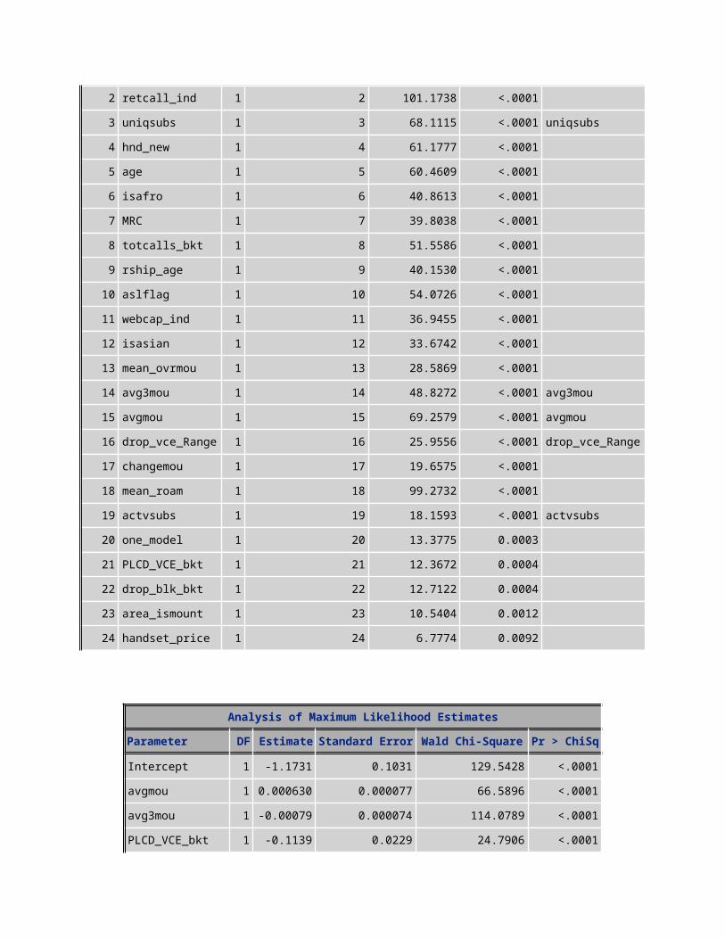
1 eqp_age 1 1 300.8859 <.0001 2 retcall_ind 1 2 101.1738 <.0001 3 uniqsubs 1 3 68.1115 <.0001 uniqsubs 4 hnd_new 1 4 61.1777 <.0001 5 age 1 5 60.4609 <.0001 6 isafro 1 6 40.8613 <.0001 7 MRC 1 7 39.8038 <.0001 8 totcalls_bkt 1 8 51.5586 <.0001 9 rship_age 1 9 40.1530 <.0001
10 aslflag 1 10 54.0726 <.0001 11 webcap_ind 1 11 36.9455 <.0001 12 isasian 1 12 33.6742 <.0001 13 mean_ovrmou 1 13 28.5869 <.0001 14 avg3mou 1 14 48.8272 <.0001 avg3mou 15 avgmou 1 15 69.2579 <.0001 avgmou 16 drop_vce_Range 1 16 25.9556 <.0001 drop_vce_Range17 changemou 1 17 19.6575 <.0001 18 mean_roam 1 18 99.2732 <.0001 19 actvsubs 1 19 18.1593 <.0001 actvsubs 20 one_model 1 20 13.3775 0.0003

21 PLCD_VCE_bkt 1 21 12.3672 0.0004 22 drop_blk_bkt 1 22 12.7122 0.0004 23 area_ismount 1 23 10.5404 0.0012 24 handset_price 1 24 6.7774 0.0092
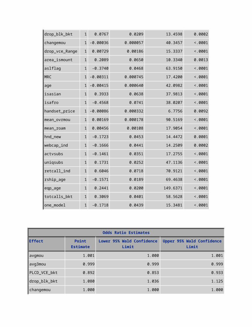
Analysis of Maximum Likelihood EstimatesParameter DF Estimate Standard Error Wald Chi-Square Pr > ChiSq
Intercept 1 -1.1731 0.1031 129.5428 <.0001avgmou 1 0.000630 0.000077 66.5896 <.0001avg3mou 1 -0.00079 0.000074 114.0789 <.0001PLCD_VCE_bkt 1 -0.1139 0.0229 24.7906 <.0001drop_blk_bkt 1 0.0767 0.0209 13.4598 0.0002changemou 1 -0.00036 0.000057 40.3457 <.0001drop_vce_Range 1 0.00729 0.00186 15.3337 <.0001area_ismount 1 0.2089 0.0650 10.3340 0.0013aslflag 1 -0.3740 0.0468 63.9150 <.0001MRC 1 -0.00311 0.000745 17.4200 <.0001age 1 -0.00415 0.000640 42.0982 <.0001isasian 1 0.3933 0.0638 37.9813 <.0001isafro 1 -0.4568 0.0741 38.0207 <.0001handset_price 1 -0.00086 0.000332 6.7756 0.0092mean_ovrmou 1 0.00169 0.000178 90.5169 <.0001mean_roam 1 0.00456 0.00108 17.9054 <.0001hnd_new 1 -0.1723 0.0453 14.4472 0.0001webcap_ind 1 -0.1666 0.0441 14.2509 0.0002actvsubs 1 -0.1461 0.0351 17.2755 <.0001uniqsubs 1 0.1731 0.0252 47.1136 <.0001retcall_ind 1 0.6046 0.0718 70.9121 <.0001rship_age 1 -0.1571 0.0189 69.4638 <.0001eqp_age 1 0.2441 0.0200 149.6371 <.0001totcalls_bkt 1 0.3069 0.0401 58.5628 <.0001one_model 1 -0.1718 0.0439 15.3481 <.0001

Odds Ratio EstimatesEffect Point
EstimateLower 95% Wald Confidence
LimitUpper 95% Wald Confidence Limit
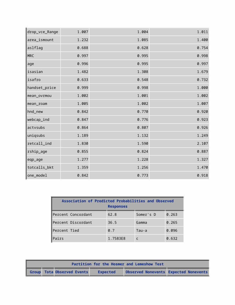
avgmou 1.001 1.000 1.001avg3mou 0.999 0.999 0.999PLCD_VCE_bkt 0.892 0.853 0.933drop_blk_bkt 1.080 1.036 1.125changemou 1.000 1.000 1.000drop_vce_Range 1.007 1.004 1.011area_ismount 1.232 1.085 1.400aslflag 0.688 0.628 0.754MRC 0.997 0.995 0.998age 0.996 0.995 0.997isasian 1.482 1.308 1.679isafro 0.633 0.548 0.732handset_price 0.999 0.998 1.000mean_ovrmou 1.002 1.001 1.002mean_roam 1.005 1.002 1.007hnd_new 0.842 0.770 0.920webcap_ind 0.847 0.776 0.923actvsubs 0.864 0.807 0.926uniqsubs 1.189 1.132 1.249retcall_ind 1.830 1.590 2.107rship_age 0.855 0.824 0.887eqp_age 1.277 1.228 1.327totcalls_bkt 1.359 1.256 1.470one_model 0.842 0.773 0.918
Association of Predicted Probabilities and Observed Responses
Percent Concordant 62.8 Somer's D 0.263Percent Discordant 36.5 Gamma 0.265
Percent Tied 0.7 Tau-a 0.096Pairs 1.7583E8 c 0.632
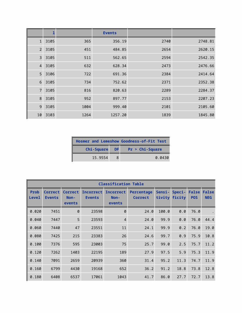
Partition for the Hosmer and Lemeshow TestGroup Total Observed
EventsExpected Events
Observed Nonevents
Expected Nonevents
1 3105 365 356.19 2740 2748.812 3105 451 484.85 2654 2620.153 3105 511 562.65 2594 2542.354 3105 632 628.34 2473 2476.665 3106 722 691.36 2384 2414.646 3105 734 752.62 2371 2352.387 3105 816 820.63 2289 2284.378 3105 952 897.77 2153 2207.239 3105 1004 999.40 2101 2105.60
10 3103 1264 1257.20 1839 1845.80
Hosmer and Lemeshow Goodness-of-Fit TestChi-Square DF Pr > Chi-Square
15.9554 8 0.0430
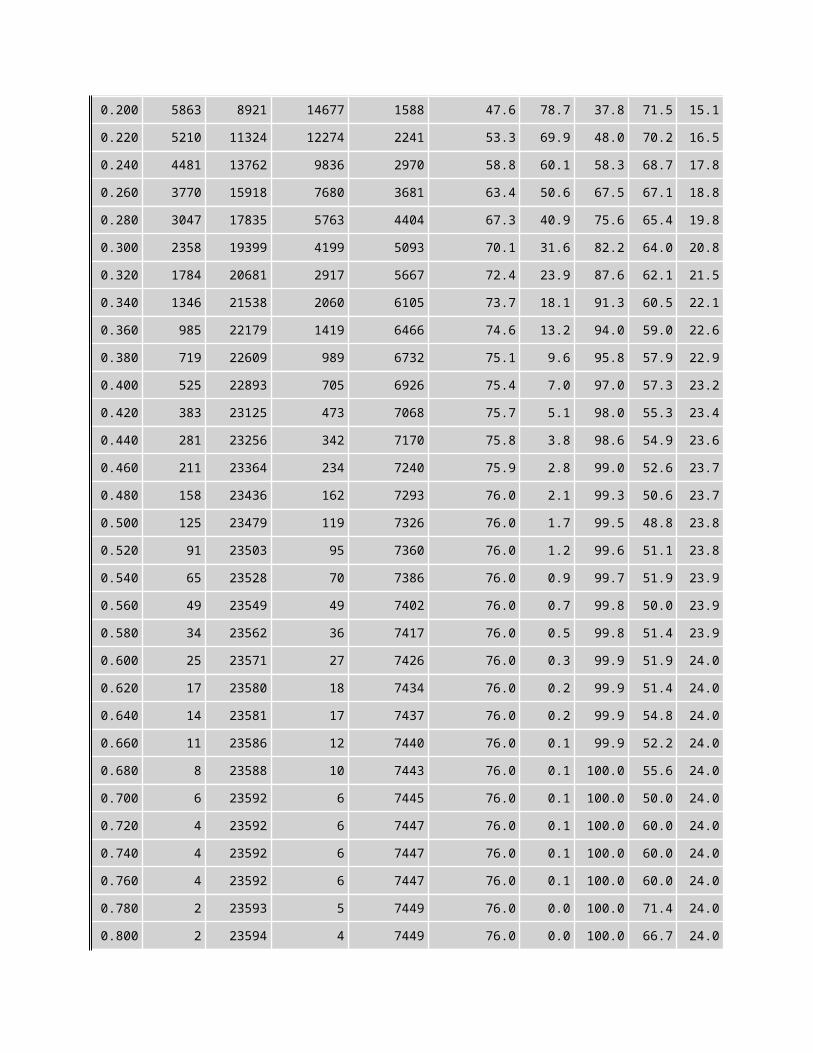
Classification TableProb Level
Correct Events
Correct Non-
events
Incorrect Events
Incorrect Non-
events
Percentage Correct
Sensi- tivity
Speci- ficity
False POS
False NEG
0.020 7451 0 23598 0 24.0 100.0 0.0 76.0 . 0.040 7447 5 23593 4 24.0 99.9 0.0 76.0 44.40.060 7440 47 23551 11 24.1 99.9 0.2 76.0 19.00.080 7425 215 23383 26 24.6 99.7 0.9 75.9 10.80.100 7376 595 23003 75 25.7 99.0 2.5 75.7 11.20.120 7262 1403 22195 189 27.9 97.5 5.9 75.3 11.9
0.140 7091 2659 20939 360 31.4 95.2 11.3 74.7 11.90.160 6799 4430 19168 652 36.2 91.2 18.8 73.8 12.80.180 6408 6537 17061 1043 41.7 86.0 27.7 72.7 13.80.200 5863 8921 14677 1588 47.6 78.7 37.8 71.5 15.10.220 5210 11324 12274 2241 53.3 69.9 48.0 70.2 16.50.240 4481 13762 9836 2970 58.8 60.1 58.3 68.7 17.80.260 3770 15918 7680 3681 63.4 50.6 67.5 67.1 18.80.280 3047 17835 5763 4404 67.3 40.9 75.6 65.4 19.80.300 2358 19399 4199 5093 70.1 31.6 82.2 64.0 20.80.320 1784 20681 2917 5667 72.4 23.9 87.6 62.1 21.50.340 1346 21538 2060 6105 73.7 18.1 91.3 60.5 22.10.360 985 22179 1419 6466 74.6 13.2 94.0 59.0 22.60.380 719 22609 989 6732 75.1 9.6 95.8 57.9 22.90.400 525 22893 705 6926 75.4 7.0 97.0 57.3 23.20.420 383 23125 473 7068 75.7 5.1 98.0 55.3 23.40.440 281 23256 342 7170 75.8 3.8 98.6 54.9 23.60.460 211 23364 234 7240 75.9 2.8 99.0 52.6 23.70.480 158 23436 162 7293 76.0 2.1 99.3 50.6 23.70.500 125 23479 119 7326 76.0 1.7 99.5 48.8 23.80.520 91 23503 95 7360 76.0 1.2 99.6 51.1 23.80.540 65 23528 70 7386 76.0 0.9 99.7 51.9 23.90.560 49 23549 49 7402 76.0 0.7 99.8 50.0 23.90.580 34 23562 36 7417 76.0 0.5 99.8 51.4 23.90.600 25 23571 27 7426 76.0 0.3 99.9 51.9 24.00.620 17 23580 18 7434 76.0 0.2 99.9 51.4 24.00.640 14 23581 17 7437 76.0 0.2 99.9 54.8 24.00.660 11 23586 12 7440 76.0 0.1 99.9 52.2 24.00.680 8 23588 10 7443 76.0 0.1 100.0 55.6 24.00.700 6 23592 6 7445 76.0 0.1 100.0 50.0 24.00.720 4 23592 6 7447 76.0 0.1 100.0 60.0 24.00.740 4 23592 6 7447 76.0 0.1 100.0 60.0 24.00.760 4 23592 6 7447 76.0 0.1 100.0 60.0 24.00.780 2 23593 5 7449 76.0 0.0 100.0 71.4 24.00.800 2 23594 4 7449 76.0 0.0 100.0 66.7 24.0

0.820 1 23594 4 7450 76.0 0.0 100.0 80.0 24.00.840 1 23595 3 7450 76.0 0.0 100.0 75.0 24.00.860 0 23595 3 7451 76.0 0.0 100.0 100.0 24.00.880 0 23595 3 7451 76.0 0.0 100.0 100.0 24.00.900 0 23597 1 7451 76.0 0.0 100.0 100.0 24.00.920 0 23597 1 7451 76.0 0.0 100.0 100.0 24.00.940 0 23597 1 7451 76.0 0.0 100.0 100.0 24.00.960 0 23597 1 7451 76.0 0.0 100.0 100.0 24.00.980 0 23597 1 7451 76.0 0.0 100.0 100.0 24.01.000 0 23598 0 7451 76.0 0.0 100.0 . 24.0
/**Generating gain chart*/
PROC LOGISTIC DATA = final.telecom2 DESCENDING OUTMODEL = DMM ;MODEL CHURN = AVGMOU AVG3MOU plcd_vce_bkt drop_blk_bkt changemou drop_vce_range DROP_VCE_MEAN area_ismount aslflag mrc age isasian ishisp isafro handset_price mean_ovrmou mean_roam hnd_new no_child webcap_ind actvsubs uniqsubs retcall_ind rship_age eqp_age totcalls_bkt one_model / ctable lackfit; SCORE OUT = DMP;RUN;
The WPS SystemThe LOGISTIC Procedure
Model Information
Data Set FINAL.telecom2Response Variable churnNumber of Response Levels 2Model binary logitOptimisation Technique Fisher's scoring
Model: This is Binary logit regression model that was fit to the data
Optimization Technique: Fishers’ scoring is the iterative method of estimating the regression parameters
Number of Observations Read 66285
Number of Observations Used 64123
The number of observations are used less than the number of observations read since there are missing values for variables used
Response ProfileOrdered Value churn Total
Frequency1 1 153172 0 48806
Probability modeled is churn='1'.
Ordered value: A descending order high to low is treated such that when the logit regression coefficients corresponds to a positive relationship for high write status, and a negative coefficients has a negative relationship with high write status . The total frequency of probability of churn is 15317 (24%) and non-probability of churn is 48806 (76%)
Model Convergence StatusConvergence criterion (GCONV=1e-008) satisfied.
The default criterion is used to assess is the relative gradient convergence criterion (GCONV) and the default precision is 10^-8. In this model the convergence criterion satisfied
Model Fit StatisticsCriterion Intercept only Intercept and CovariatesAIC 70508.162 68071.173SC 70517.230 68325.093-2 Log L 70506.162 68015.173
AIC: Akaike Information Criterion is used for the comparison of non nested models on the same sample. The model with low AIC will be the best.
SC: if The Schwarz Criterion is small and that is most desirable
AIC and SC penalize the log- likelihood by the number of predictors in the model
The -2 Log L is used in hypothesis tests for nested models and this is negative two times the log likelihood
Intercept and Covariates: A fitted model includes all independent variables and the intercept. This can be compared the values in this column with the criteria corresponding intercept only value to assess modelfit/significance
Testing Global Null Hypothesis: BETA=0Test Chi-Square DF Pr > Chi-SquareLikelihood Ratio 2490.9885 27 <.0001

Score 2453.9078 27 <.0001Wald 2316.9133 27 <.0001
The Global null hypothesis test against null hypothesis that at least one of the predictor’s regression coefficient is not equal to zero
Likelihood Ratio, score and wald test that at least one of the predictor’s regression coefficient is not equal to zero
Calculations: - 2 Log L (Null model which is intercept only) – 2 Log L (fitted model which is intercept and covariates) which 2490.9885
PR>Chi-Square: it is compared to specified alpha level and accept the a type 1 error. The small p value lead to conclude that at least one of the regression coefficients in the model is not equal to zero
Analysis of Maximum Likelihood EstimatesParameter DF Estimate Standard Error Wald Chi-Square Pr > ChiSqIntercept 1 -1.1379 0.0715 253.0321 <.0001avgmou 1 0.000602 0.000054 123.5508 <.0001avg3mou 1 -0.00073 0.000053 193.1890 <.0001PLCD_VCE_bkt 1 -0.1156 0.0160 52.0034 <.0001drop_blk_bkt 1 0.0654 0.0149 19.2666 <.0001changemou 1 -0.00035 0.000039 81.3616 <.0001drop_vce_Range 1 0.00408 0.00166 6.0576 0.0138drop_vce_Mean 1 0.00500 0.00182 7.5236 0.0061area_ismount 1 0.2289 0.0458 25.0235 <.0001aslflag 1 -0.4061 0.0324 156.7115 <.0001MRC 1 -0.00308 0.000518 35.4324 <.0001age 1 -0.00426 0.000457 86.9453 <.0001isasian 1 0.3287 0.0455 52.0675 <.0001ishisp 1 0.0683 0.0280 5.9410 0.0148isafro 1 -0.3722 0.0500 55.3905 <.0001handset_price 1 -0.00107 0.000233 21.1778 <.0001mean_ovrmou 1 0.00155 0.000124 155.9362 <.0001mean_roam 1 0.00421 0.000725 33.8267 <.0001hnd_new 1 -0.1494 0.0319 21.9503 <.0001no_child 1 -0.0777 0.0331 5.5112 0.0189

webcap_ind 1 -0.1548 0.0308 25.2265 <.0001actvsubs 1 -0.1258 0.0243 26.7277 <.0001uniqsubs 1 0.1546 0.0173 79.6071 <.0001retcall_ind 1 0.7068 0.0489 209.1117 <.0001rship_age 1 -0.1507 0.0132 130.8075 <.0001eqp_age 1 0.2531 0.0137 340.3424 <.0001totcalls_bkt 1 0.2621 0.0279 88.1317 <.0001one_model 1 -0.1533 0.0304 25.4935 <.0001
Parameter – the predictor variables in the model and intercept
DF: Degrees of Freedom corresponding to the parameter. Each parameter estimated in the model requires one DF(which is estimated in this model as one) and defines the Chi-square distribution to test whether the individual regression coefficient is zero, given the other variables are in the model.
Estimate: These are the binary logit regression estimates for the parameters in the model. The logistic regression model models the log odds of a positive response (churn probability = 1) as a linear combination the predictor variables.
Log(P/1-p) = b0+b1*pv+b2*pv+b3*pv…
Log (p/1-p) = -1.1379+(0.000602*avgmou)+(-0.00073*avg3mou)+…….
Interpretation: For a unit change in the predictor variable, the difference in log-odds for a positive outcome is expected to change by the respective coefficient given the other variables in the model are held constant.
Intercept = -1.1379 (logistic regression estimate when all variables in the model are evaluated at zero.
Standard error – these are the standard errors of the individual regression coefficients.
Pr>ChiSq : Testing the null hypothesis that an individual predictor’s regression coefficient is zero,given the other predictor variables are in the model. The chi square test statistic is the squared ration of the estimate to the standard error of the respective predictor. In this model all variables are significant at 0.05 %
Odds Ratio EstimatesEffect Point
EstimateLower 95% Wald Confidence
LimitUpper 95% Wald Confidence Limit
avgmou 1.001 1.000 1.001avg3mou 0.999 0.999 0.999PLCD_VCE_bkt 0.891 0.863 0.919drop_blk_bkt 1.068 1.037 1.099changemou 1.000 1.000 1.000drop_vce_Range 1.004 1.001 1.007drop_vce_Mean 1.005 1.001 1.009area_ismount 1.257 1.149 1.375
aslflag 0.666 0.625 0.710MRC 0.997 0.996 0.998age 0.996 0.995 0.997isasian 1.389 1.270 1.519ishisp 1.071 1.013 1.131isafro 0.689 0.625 0.760handset_price 0.999 0.998 0.999mean_ovrmou 1.002 1.001 1.002mean_roam 1.004 1.003 1.006hnd_new 0.861 0.809 0.917no_child 0.925 0.867 0.987webcap_ind 0.857 0.806 0.910actvsubs 0.882 0.841 0.925uniqsubs 1.167 1.128 1.207retcall_ind 2.028 1.842 2.231rship_age 0.860 0.838 0.883eqp_age 1.288 1.254 1.323totcalls_bkt 1.300 1.230 1.373one_model 0.858 0.808 0.910
Points Effect: The odds ratio is obtained by exponentiation the estimate. These difference in the log of two odds is equal to the log of the ration of these two odds. The log of the ration of the two odds is the log odds ratio.
Interpretation: For a one unit change in the predictor variable, the odds ratio for a positive outcome is expected to change by the respective coefficient, given the other variables in the model are held constant.
95% Wald Confidence Limits: This is the Wald Confidence Interval (CI) of an individual odds ratio, given the other predictor’s variables are in the model. For a given predictor variable with a level of 95% confidence, that we are 95% confident that upon repeated trials, 95% of the CI’s include the true population odds ratio. If the CI includes one we would fail to reject the null hypothesis that a particular regression coefficient equals to zero and the odds ration equals one, given the other predictors are in the model.
Association of Predicted Probabilities and Observed Responses
Percent Concordant 63.0 Somer's D 0.267Percent Discordant 36.3 Gamma 0.268Percent Tied 0.7 Tau-a 0.097Pairs 7.4756E8 c 0.633
Percent Concordant: A pair of observations with different observed responses is said to be concordant if the observation with the lower ordered response value “0” has a lower predicted mean score than the observation with the higher ordered response value “1”. The concordant percent is 63 %. The higher the
concordant the better the model is. This looks a good model since the concordant value is higher than the discordant percent.
Percent Discordant: If the observation with the lower ordered response value has a higher predicted mean score than the observation with the higher ordered response value. The discordant percent is 36.3%
Percent Tied: It is ties since a pair of observations is neither concordant nor discordant.
Pairs: The total number of distinct pairs in which one case has an observed outcome different from the other member of the pair.
In the response profile table we have 15317 observations with honcomp = 1 and 48806 observations with honcomp = 0; This the total number of pairs with different coutcomes is 15317*48806 = 747,561,502 (7.4756E8)
Somer’s D: Is used to determine the strength and direction of relation between pairs of variables values ranges from -1 (all pairs disagree) to 1 (all pairs agree). It is defined as (concordant – discordant)/number of total number of pairs with different response
Somer’s D = (63-36.3)/100 = 0.267
Gamma : The Good man – Kruskal Gamma method does not penalize for ties on either variable. It value ranges from -1(no association) to 1 (perfect association). It generally is greater than Somer’s D
Tau-a: Kendall’s Tau-a is a modification of Somer’s D that takes into account the difference between the number of possible paired observations and the number of paired observations with a different response. It is defined to be the ratio of the difference between the number of concordant pairs and the number of discordant pairs to the number of possible pairs. Usually Tau-a is much smaller than Somer’s D since there would be many paired observations with the same response.
C-C: This is equivalent to the well known measure ROC. C ranges from 0.5 to 1 where 0.5 corresponds to the model randomly predicting the response, and a 1 corresponds to the model perfectly discriminating the response.
Partition for the Hosmer and Lemeshow TestGroup Total Observed
EventsExpected Events
Observed Nonevents
Expected Nonevents
1 6413 750 731.23 5663 5681.772 6412 905 980.93 5507 5431.073 6413 1117 1143.90 5296 5269.104 6412 1228 1284.09 5184 5127.915 6412 1423 1416.34 4989 4995.666 6412 1555 1549.39 4857 4862.617 6412 1702 1691.44 4710 4720.568 6412 1914 1854.05 4498 4557.959 6412 2107 2064.37 4305 4347.63
10 6413 2616 2601.28 3797 3811.72
Hosmer and Lemeshow Goodness-of-Fit TestChi-Square DF Pr > Chi-Square
15.6395 8 0.0478
1. Hosmer and Lemeshow Goodness-of-Fit Test –
Pr > Chi-square value is 0.0478 which is higher than that of the training dataset and validation dataset respectively 0.0430 and 0.0428 as well as lower than 0.05 indicating a good model.
2. Association of Predicted Probabilities and Observed Responses
Percent Concordant is 63 (62.8 of training dataset) and percent discordant is 36.3 (36.5 of the training dataset). This is an acceptable score. There is an improvement over the training dataset
Classification TableProb Level
Correct Events
Correct Non-
events
Incorrect Events
Incorrect Non-
events
Percentage Correct
Sensi- tivity
Speci- ficity
False POS
False NEG
0.020 15317 0 48806 0 23.9 100.0 0.0 76.1 . 0.040 15313 7 48799 4 23.9 100.0 0.0 76.1 36.40.060 15300 80 48726 17 24.0 99.9 0.2 76.1 17.50.080 15262 372 48434 55 24.4 99.6 0.8 76.0 12.90.100 15161 1195 47611 156 25.5 99.0 2.4 75.8 11.50.120 14921 3024 45782 396 28.0 97.4 6.2 75.4 11.60.140 14522 5955 42851 795 31.9 94.8 12.2 74.7 11.80.160 13870 9766 39040 1447 36.9 90.6 20.0 73.8 12.90.180 13020 14161 34645 2297 42.4 85.0 29.0 72.7 14.00.200 11967 18992 29814 3350 48.3 78.1 38.9 71.4 15.00.220 10673 23896 24910 4644 53.9 69.7 49.0 70.0 16.30.240 9246 28702 20104 6071 59.2 60.4 58.8 68.5 17.50.260 7758 33074 15732 7559 63.7 50.6 67.8 67.0 18.60.280 6338 36968 11838 8979 67.5 41.4 75.7 65.1 19.50.300 4929 40169 8637 10388 70.3 32.2 82.3 63.7 20.50.320 3733 42750 6056 11584 72.5 24.4 87.6 61.9 21.30.340 2770 44637 4169 12547 73.9 18.1 91.5 60.1 21.90.360 2057 45943 2863 13260 74.9 13.4 94.1 58.2 22.40.380 1521 46808 1998 13796 75.4 9.9 95.9 56.8 22.80.400 1122 47432 1374 14195 75.7 7.3 97.2 55.0 23.00.420 808 47806 1000 14509 75.8 5.3 98.0 55.3 23.3
0.440 605 48088 718 14712 75.9 3.9 98.5 54.3 23.40.460 451 48295 511 14866 76.0 2.9 99.0 53.1 23.50.480 340 48425 381 14977 76.0 2.2 99.2 52.8 23.60.500 260 48511 295 15057 76.1 1.7 99.4 53.2 23.70.520 193 48596 210 15124 76.1 1.3 99.6 52.1 23.70.540 140 48642 164 15177 76.1 0.9 99.7 53.9 23.80.560 93 48691 115 15224 76.1 0.6 99.8 55.3 23.80.580 67 48727 79 15250 76.1 0.4 99.8 54.1 23.80.600 47 48742 64 15270 76.1 0.3 99.9 57.7 23.90.620 30 48761 45 15287 76.1 0.2 99.9 60.0 23.90.640 22 48770 36 15295 76.1 0.1 99.9 62.1 23.90.660 16 48777 29 15301 76.1 0.1 99.9 64.4 23.90.680 11 48782 24 15306 76.1 0.1 100.0 68.6 23.90.700 7 48789 17 15310 76.1 0.0 100.0 70.8 23.90.720 6 48791 15 15311 76.1 0.0 100.0 71.4 23.90.740 5 48793 13 15312 76.1 0.0 100.0 72.2 23.90.760 3 48795 11 15314 76.1 0.0 100.0 78.6 23.90.780 2 48797 9 15315 76.1 0.0 100.0 81.8 23.90.800 2 48798 8 15315 76.1 0.0 100.0 80.0 23.90.820 1 48800 6 15316 76.1 0.0 100.0 85.7 23.90.840 1 48801 5 15316 76.1 0.0 100.0 83.3 23.90.860 1 48801 5 15316 76.1 0.0 100.0 83.3 23.90.880 1 48803 3 15316 76.1 0.0 100.0 75.0 23.90.900 1 48803 3 15316 76.1 0.0 100.0 75.0 23.90.920 0 48803 3 15317 76.1 0.0 100.0 100.0 23.90.940 0 48804 2 15317 76.1 0.0 100.0 100.0 23.90.960 0 48804 2 15317 76.1 0.0 100.0 100.0 23.90.980 0 48805 1 15317 76.1 0.0 100.0 100.0 23.91.000 0 48806 0 15317 76.1 0.0 100.0 . 23.9
/*Ranking the data*/PROC RANK DATA = DMP OUT = final.DECILE GROUPS = 10 TIES = MEAN ;VAR p_1;RANKS decile;RUN;
PROC SORT DATA = final.DECILE ;
BY DESCENDING p_1 ;RUN;
EXPORT THE DATA
PROC EXPORT DATA = final.DECILEOUTFILE = 'Y:\Programes\SAS Graded Assignment\Final Case Study\Gain.xlsx'DBMS = EXCEL;RUN;
Accuracy
/*check accuracy**/
Data final.testacc;set DMP;if f_churn = 0 and i_churn = 0 then out = "True Negative";else if f_churn = 1 and i_churn = 1 then out = "True Positive";else if f_churn = 0 and i_churn = 1 then out = "False Positive";else if f_churn = 1 and i_churn = 0 then out = "False Negative";run;
Proc freq;tables out;run;
Cut off probability = 0.5
out Frequency
Percent Cumulative
Frequency
Cumulative
Percent
Predicted Actual ExpectedFalse Negativ 15055 23.48 15055 23.48
64123 Churn = 0 Churn = 1False Positiv 293 0.46 15348 23.94
Churn = 0 48511 15057
True Negative
48513 75.66 63861 99.59
Churn = 1 260 295True Positive 262 0.41 64123 100
True NegativeTrue PositiveFalse Positve False Negative76% 0.46% 23.48% 0.41%
P_Churn = 0 and A_Churn = 0 then True Negative%yes captured correctly 0.46% P_Churn = 1 and A_Churn = 1 then True Positive%of actual nos missclassfied as yes 76% P_Churn = 0 and A_Churn = 1 then False Positive%of Nos captured correctly 0.41% P_Churn = 1 and A_Churn = 0 then False Negative% of actual yes missclassified as Nos = 24%
Frequency Missing = 2162
out Frequency Percent Cumulative Frequency
Cumulative Percent
False Negativ 15055 23.48 15055 23.48False Positiv 293 0.46 15348 23.94
True Negative 48513 75.66 63861 99.59True Positive 262 0.41 64123 100.00
Frequency Missing = 2162
Gain Chart:
Sum of churn Average of P_1 Count of P_1 Sum of P_1_2 Expected ChurnCumulative expcted churn Predicted churnCumulative predicted churnLift by mode2616 0.405634825 6412 2600.930497 1531.7 10% 0.169807 17% 1.7079062107 0.321959928 6412 2064.407059 1531.7 20% 0.134779 30% 1.3755961914 0.289155258 6413 1854.352672 1531.7 30% 0.121065 43% 1.2495921702 0.26379269 6412 1691.43873 1531.7 40% 0.110429 54% 1.1111841555 0.241637261 6413 1549.619755 1531.7 50% 0.10117 64% 1.0152121423 0.220886158 6412 1416.322048 1531.7 60% 0.092467 73% 0.9290331228 0.200260533 6412 1284.070538 1531.7 70% 0.083833 81% 0.8017241117 0.178368073 6413 1143.874452 1531.7 80% 0.07468 89% 0.729255
906 0.152979779 6412 980.9063447 1531.7 90% 0.06404 95% 0.5915749 0.114019516 6412 731.0931359 1531.7 100% 0.047731 100% 0.488999
15317 0.238869286 64123 15317.01523 15317
Cumulative Expected Cumulative Predicted10% 17%20% 30%30% 43%40% 54%50% 64%60% 73%70% 81%80% 89%90% 95%
100% 100%

From the gain chart, the model appears to be a better predictor than a standard average probability calculation.
At 50% probability level, the model has correctly predicted 260 churn of 15057 actual, which is only a 1.7% success rate. But it has correctly predicted 48513 out of 48775 non churn, which is 99.5% success rate.
At 50% probability level, the model has correctly predicted 295 churn of 15057 actual, which is very healthy a 1.9% success rate. It has correctly predicted 48513 out of 48808 non churn, which is 99.4% success rate. This probability level can be chosen as an appropriate level for prediction.