Filters

Workshop on Digital Signal and Image processing

Speaker: Dr. Rubaiyat Yasmin

25 May, 2012

Dept. of Information and Communication Engineering, R.U.

1

Introduction:

What is filter?Electronic circuits

To remove unwanted frequency components from the signal,

To enhance wanted ones.

Perform signal processing functions

Why needed?

2

Objective:

• Analog Filters• Digital Filters• Adaptive Filters

Basic understanding

3

Basic Types of Filters:

• Low-pass • High-pass• Band-pass • Band-reject

Four Main Filter Types:

4

Basic Types of Filters (Contd)

Pass band, H(f)=1

Stop band, H(f)=0

Cut-off frequency

5

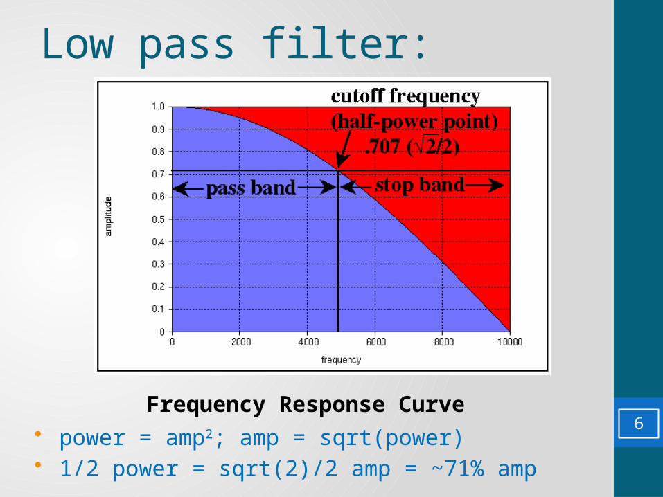
Low pass filter:

Frequency Response Curve• power = amp2; amp = sqrt(power)• 1/2 power = sqrt(2)/2 amp = ~71% amp

6

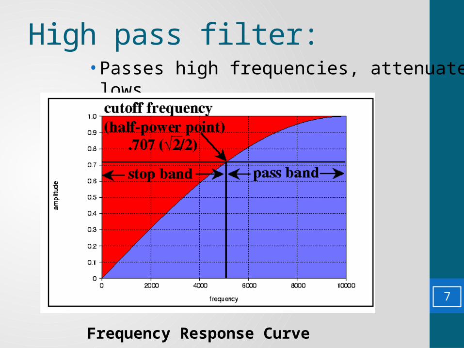
High pass filter:• Passes high frequencies, attenuates lows.

Frequency Response Curve

7

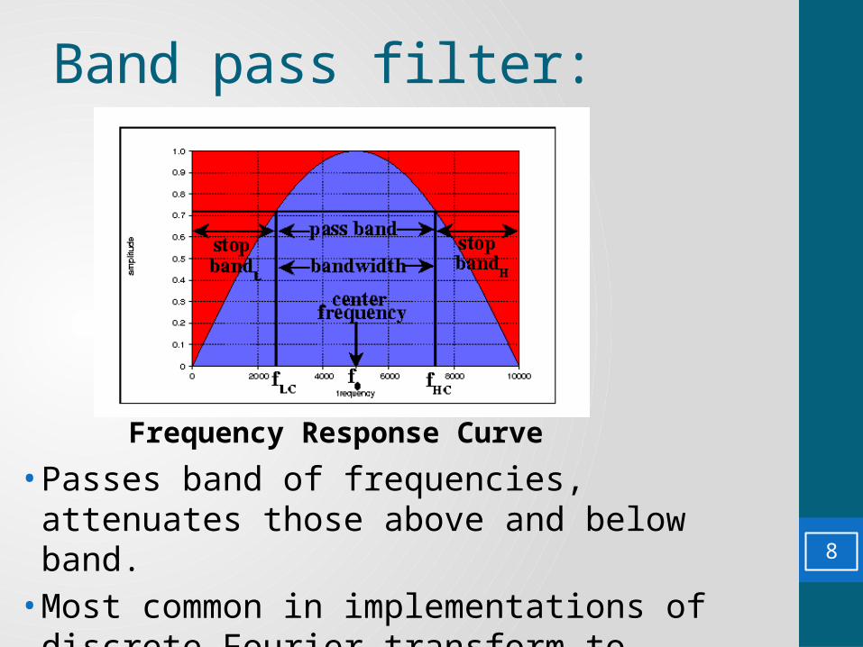
Band pass filter:

• Passes band of frequencies, attenuates those above and below band.

• Most common in implementations of discrete Fourier transform to separate out harmonics.

Frequency Response Curve

8

Band reject filter:• Stops band of frequencies, passes those above and

below band.• Most common in removing electric hum (50 Hertz A/C).

Frequency Response Curve

9

Analogue designs

• Exist for all the standard filter types (lowpass, highpass, bandpass, bandreject).

To define a standard lowpass filter, and To use standard analogue-analogue transformations from lowpass to the other types, prior to performing the bilinear transform.

Butterworth Chebyshev Elliptic

Common Approach :

Important families:

• Frequencies are specified in the Ω domain (in rad/s))

10

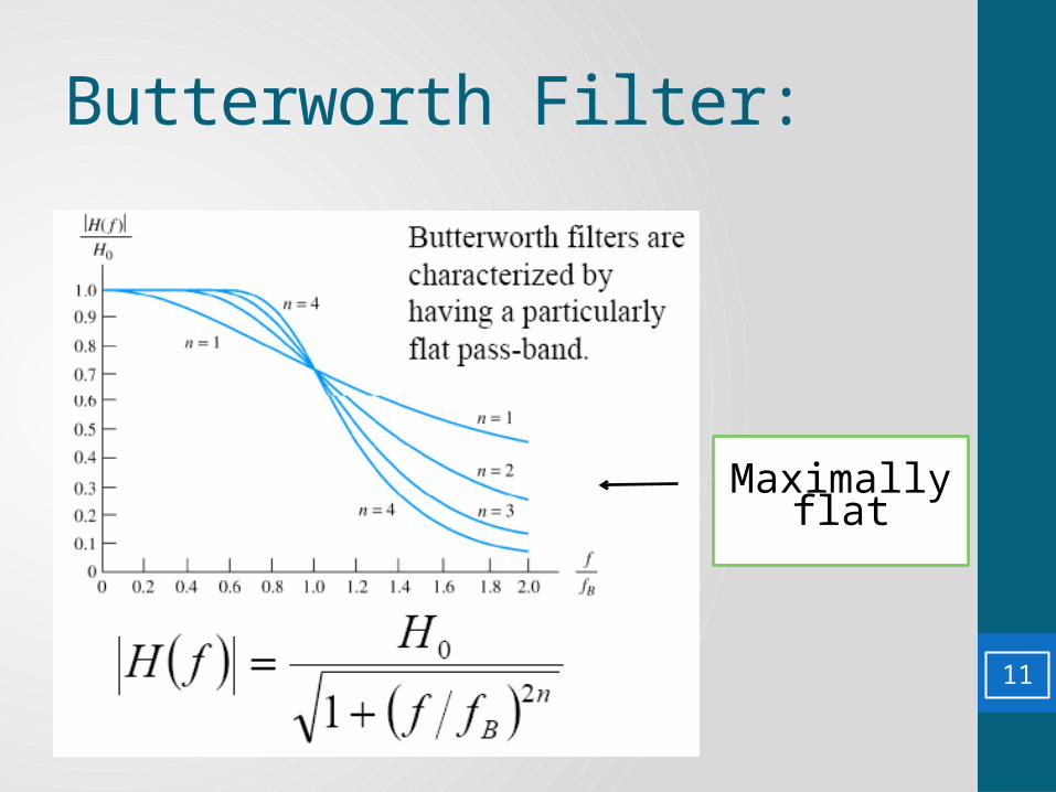
Butterworth Filter:

Maximally flat

11

Chebyshev Filter: Equiripple response in pass-band (up to ωc),

Monotonically decreasing in stop-band

12

Elliptic Filter: Equiripple in both pass-band and stop-band

13

Other Types of Analogue Filter Bessel filters, which are almost linear phase.

• Involve different degrees of flexibility and trade-offs in specifying transition bandwidth, ripple amplitude in pass-band/stop-band and phase linearity.

For a given band edge frequency, ripple specification, and filter order, narrower transition bandwidth can be traded off against worse phase linearity

14

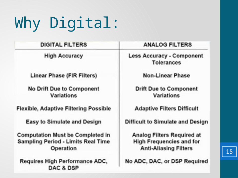
Why Digital:

15

16

Basic concept :

17

What is a Digital Filter?Digital Filter: Numerical procedure or algorithm that transforms a given sequence of numbers into a second sequence that has some more desirable properties.

Input sequencexn Digital Filter

Output sequenceyn

18

Desired features

Depend on the application, for example

Input Signal

generated by sensingdevice (microphone)

speech

Output

having less noise orinterferences

with reducedredundancy for moreefficient transmission 19

Examples of filtering operationsNoise suppression:

•  received radio signals

•  signals received by image sensors (TV,infrared imaging devices)

•  electrical signals measured from humanbody (brain heart, neurological signals)

•  signals recorded on analog media suchas analog magnetic tapes

20

Enhancement of selected frequency ranges:

•  treble and bass control or graphic equalizers

increase sound level and high and low level frequenciesto compensate for the lower sensitivity of the ear

•  enhancement of edges in imagesimprove recognition of object (by human or computer)

21

Specific operations:

•  differentiation•  integration•  Hilbert transform

These operations can beapproximated by digital filtersoperating on the sampled inputsignal

22

The Basic of Digital FiltersFilters work by using one or both of the following methods:– Delay a copy of the input signal (by x number of

samples), and combine the delayed input signal with the new input signal.• (Finite Impulse Response, FIR, or feedforward

filter)– Delay a copy of the output signal (by x number of

samples), and combine it with the new input signal.• (Infinite Impulse Response, IIR, feedback filter)

FIR Filters IIR Filters

23

FIR FiltersFIR filter of length M (order N=M-1, order - number of delays)

The Order of the filter is equal to the number of samples you look back

24

25

The impulse response is of finite length M

FIR filters have only zeros (no poles), henceknown also as all-zero filters

FIR filters also known as feedforward ornon-recursive, or transversal

Now N-point DFT (Y(k)) and then N-point IDFT (y(n)) can be usedto compute standard convolution product and thus to performlinear filtering (given how efficient FFT is)

Frequency-domain Equivalent:

26

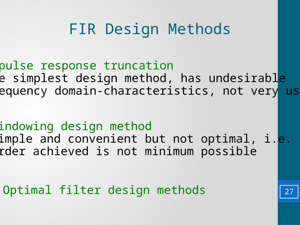
FIR Design Methods

•  Impulse response truncation the simplest design method, has undesirable frequency domain-characteristics, not very useful

•  Windowing design method simple and convenient but not optimal, i.e. order achieved is not minimum possible

•  Optimal filter design methods 27

Approximated filters obtained by truncation

28

FIR Filter Design

Consider the Window method:• Determine ideal response function• If length of ideal function is too long, multiply

ideal response by a finite length window function

• Note that multiplication by window in time domain means convolution (and smearing) in the frequency domain

29

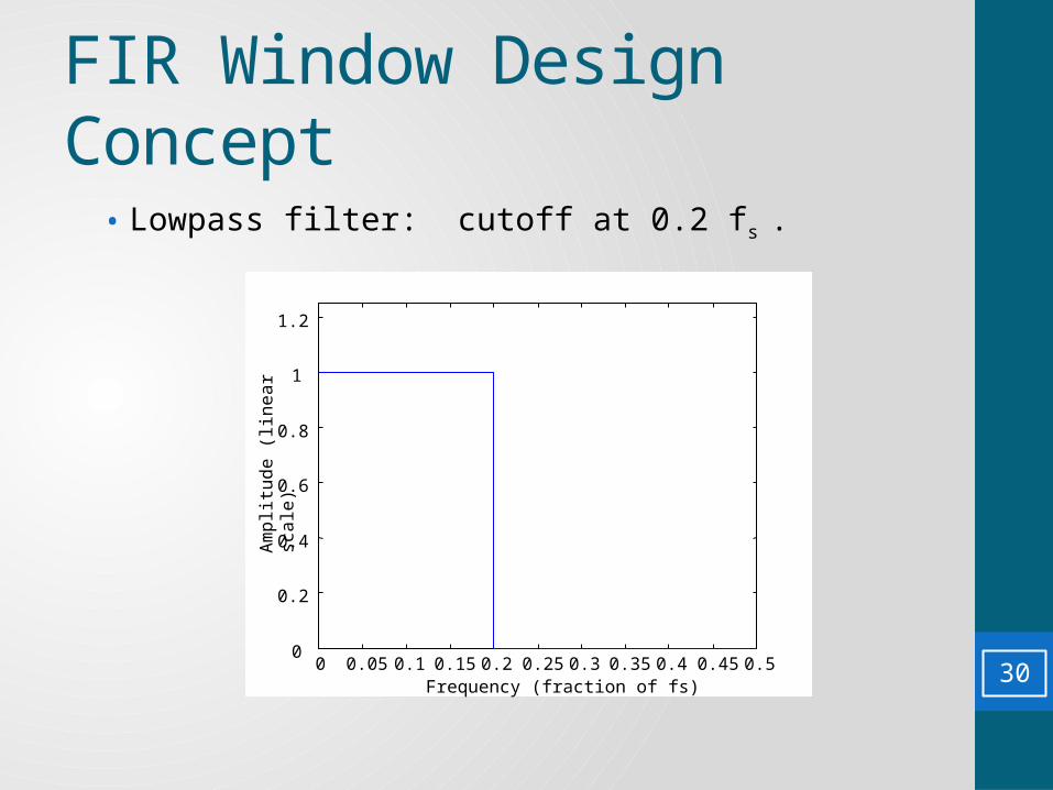
FIR Window Design Concept

• Lowpass filter: cutoff at 0.2 fs .

0 0.05 0.1 0.15 0.2 0.25 0.3 0.35 0.4 0.45 0.50

0.2

0.4

0.6

0.8

1

1.2

Frequency (fraction of fs)

Am

plit

ud

e (

line

ar

sca

le)

30

FIR Design Concept (cont.)

• Time domain response (Inverse DTFT)

-60 -40 -20 0 20 40 60-0.1

-0.05

0

0.05

0.1

0.15

0.2

0.25

0.3

0.35

0.4

Sample Index

Am

plitu

de

31

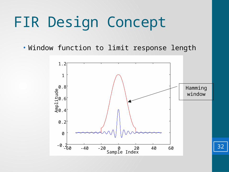
FIR Design Concept

• Window function to limit response length

-60 -40 -20 0 20 40 60-0.2

0

0.2

0.4

0.6

0.8

1

1.2

Sample Index

Am

plitu

de

Hamming window

32

FIR Design Concept (cont.)

• Windowed and shifted (causal) result

0 5 10 15 20 25 30 35 40-0.1

-0.05

0

0.05

0.1

0.15

0.2

0.25

0.3

0.35

0.4

Am

plitu

de

Sample Index33

FIR Design Concept

• Resulting frequency response of filter

0 0.05 0.1 0.15 0.2 0.25 0.3 0.35 0.4 0.45 0.5-60

-50

-40

-30

-20

-10

0

10

Frequency (fraction of fs)

Mag

nitu

de (

dB)

34

Window Design Method

Rectangular Window Frequency Response

35

Truncated Filter

Increasing the dimension of the window M: The width of the main lobe decreases The area under side lobes remain constant

36

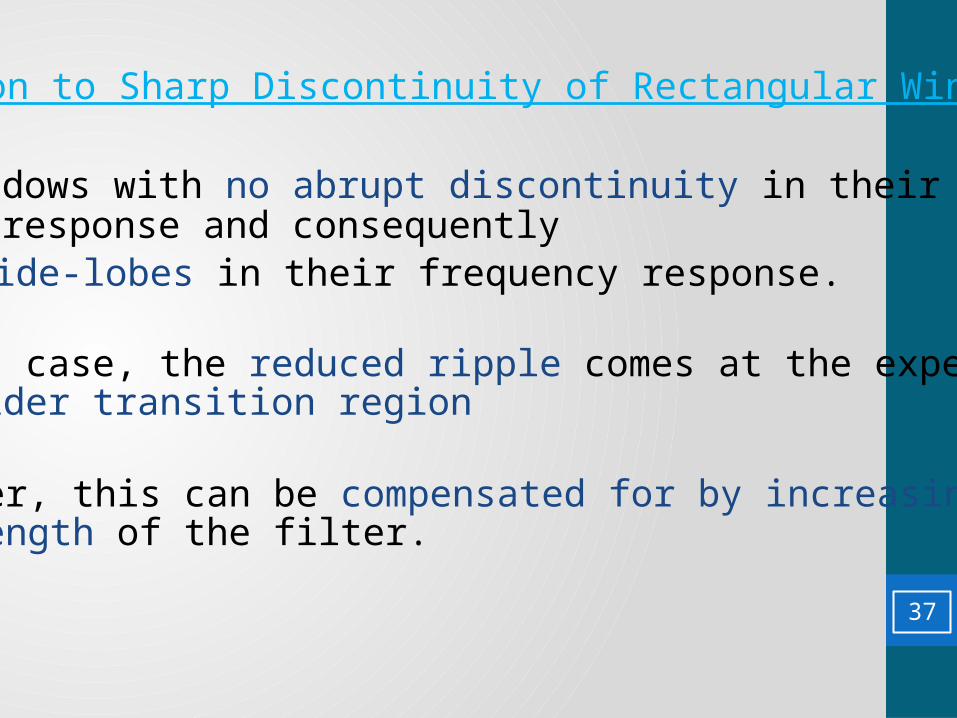
Solution to Sharp Discontinuity of Rectangular Window

Use windows with no abrupt discontinuity in their time-domain response and consequentlylow side-lobes in their frequency response.

In this case, the reduced ripple comes at the expenseof a wider transition region

However, this can be compensated for by increasingthe length of the filter.

37

Alternative Windows -Time Domain

• Hanning • Hamming • Blackman

Window Characteristics:

A wider transition region (wider main-lobe) is compensated by much lower side-lobes and thus less ripples.

38

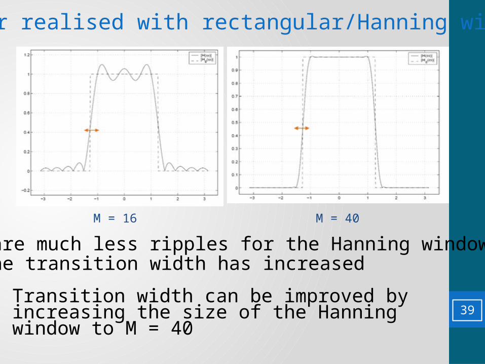
Filter realised with rectangular/Hanning window

There are much less ripples for the Hanning window butthat the transition width has increased

Transition width can be improved by increasing the size of the Hanning window to M = 40

M = 40M = 16

39

Windows characteristics

•  Fundamental trade-off between main-lobewidth and side-lobe amplitude

•  As window smoother, peak side-lobedecreases, but the main-lobe width increases.

•  Need to increase window length to achievesame transition bandwidth.

Specification necessary for Window Design Method40

Window Design Procedure

•  Ideal frequency response has infinite impulse response

•  To be implemented in practice it has to be-  truncated

-  shifted to the right (to make is causal)

•  Truncation is just pre-multiplication by a rectangular window

-  the filter of a large order has a narrow transition band

-  however, sharp discontinuity results in side-lobeinterference independent of the filter’s order andshape Gibbs phenomenon

•  Windows with no abrupt discontinuity can be used to reduceGibbs oscillations (e.g. Hanning, Hamming, Blackman)

41

Windowed FIR filter design procedure

1.  Select a suitable window function

2.  Specify an ideal response Hd(ω)

3.  Compute the coefficients of the ideal filter hd(n)

4.  Multiply the ideal coefficients by the window function togive the filter coefficients

5.  Evaluate the frequency response of the resulting filterand iterate if necessary (typically, it means increase M ifthe constraints you have been given have not been

satisfied)

42

FIR Filter Design Using Windows

FIR filter design based on windows is simple and robust,however, it is not optimal:

•  The resulting pass-band and stop-band parametersare equal even though often the specification is morestrict in the stop band than in the pass band

unnecessary high accuracy in the pass band

•  The ripple of the window is not uniform (decays as wemove away from discontinuity points according toside-lobe pattern of the window)

by allowing more freedom in the ripple behaviourwe may be able to reduce filter’s order and henceits complexity

FIR Design by Optimisation Least-Square Method

43

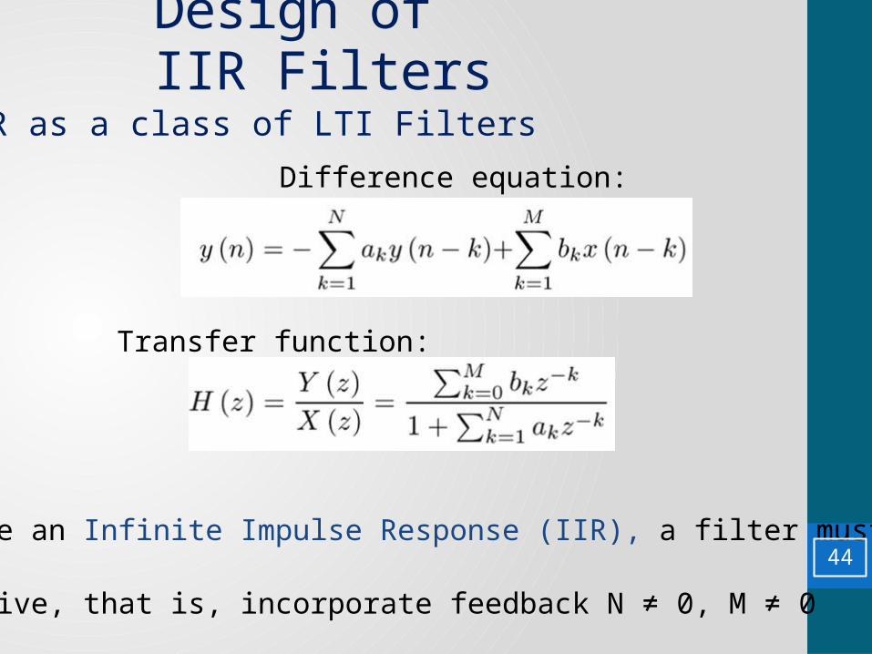
IIR as a class of LTI Filters

Difference equation:

Transfer function:

To give an Infinite Impulse Response (IIR), a filter must berecursive, that is, incorporate feedback N ≠ 0, M ≠ 0

Design of IIR Filters

44

IIR Filters Design from an Analogue Prototype

Almost all methods rely on converting an analogue filter to a digital one

Analogue to Digital Conversion:

AnalogueDigital

45

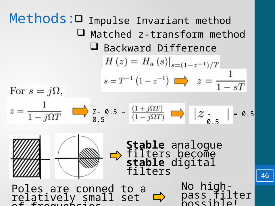
Methods: Impulse Invariant method Matched z-transform method Backward Difference Method

Z- 0.5 = 0.5 = 0.5- 0.5

Stable analogue filters become stable digital filters

Poles are conned to a relatively small set of frequencies

No high-pass filter possible!

46

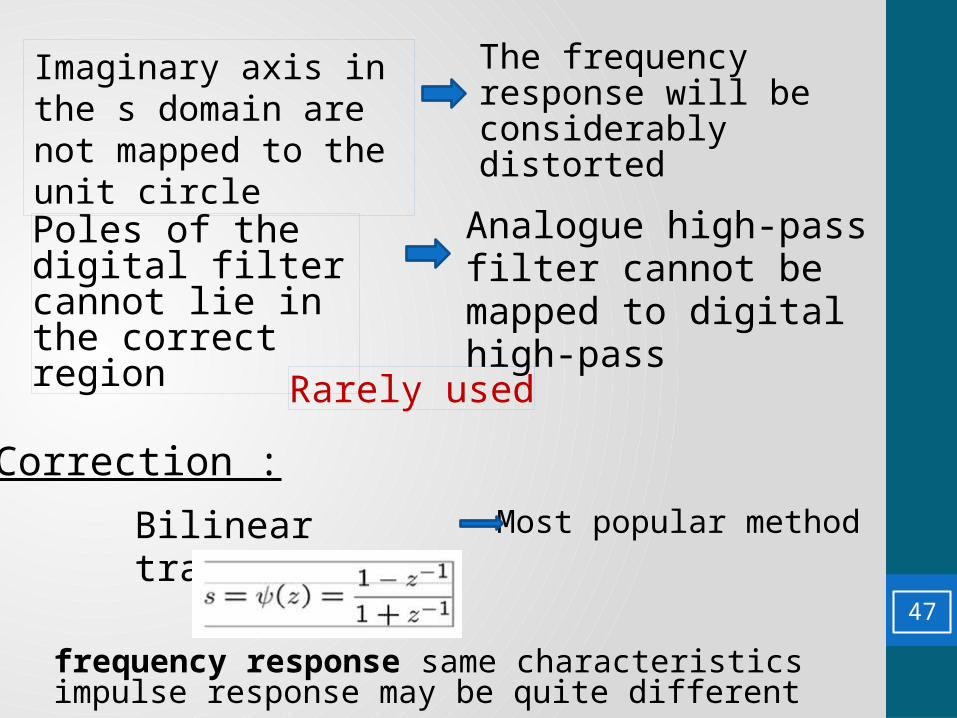
The frequency response will be considerably distorted

Analogue high-pass filter cannot be mapped to digital high-pass

Poles of the digital filter cannot lie in the correct region

Rarely used

Imaginary axis in the s domain are not mapped to the unit circle

Correction :

Bilinear transform Most popular method

frequency response same characteristicsimpulse response may be quite different

47

Two important cases:

1. With σ=0 Imaginary (frequency) axis in the s-plane maps to the unit circle in the z-plane

2. With σ <0, Left half s-plane maps onto the interior of the unit circle

Properties of the Bilinear Transform

Suitable frequency response, stability for digital filter

s-plane z-plane

48

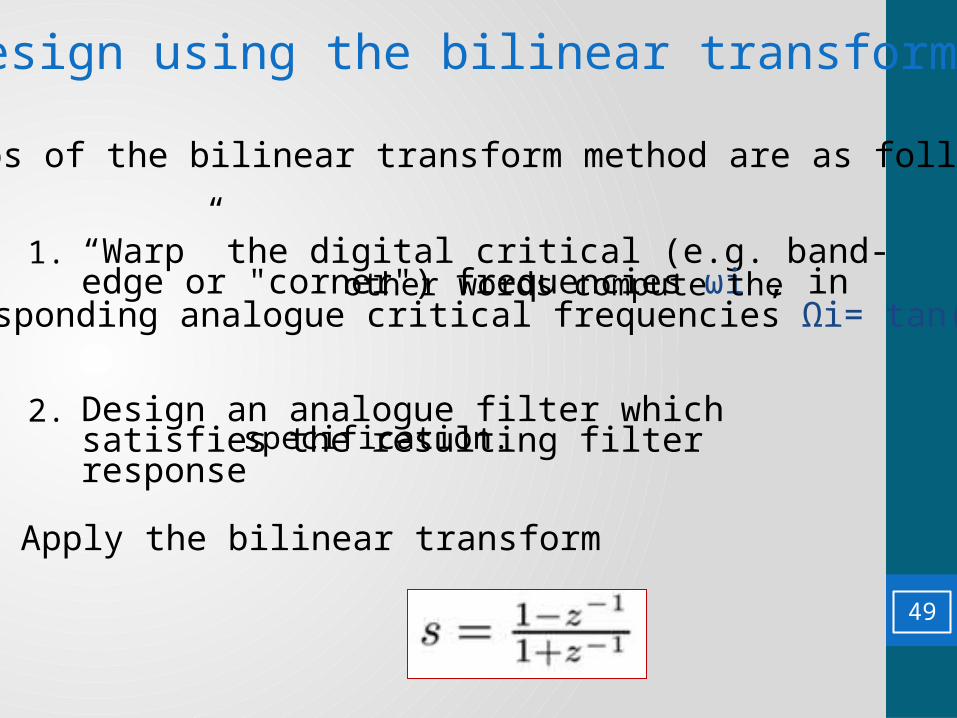
Design using the bilinear transform

The steps of the bilinear transform method are as follows:

1. “Warp” the digital critical (e.g. band-edge or "corner") frequencies ωi , in other words compute thecorresponding analogue critical frequencies Ωi= tan(ωi/2).

2. Design an analogue filter which satisfies the resulting filter response specification.

3. Apply the bilinear transform

49

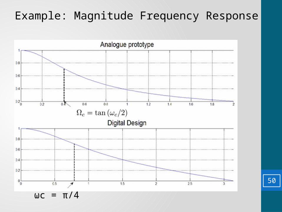
Example: Magnitude Frequency Response

ωc = π/4

50

Designing high-pass, band-pass and band-stop filters

• Various techniques available to transform a low-pass filter into a high-pass/band pass/band-stop filters.

Frequency transformation in the analogue domain

• Concentrated on IIR filters with low-passcharacteristics.

51

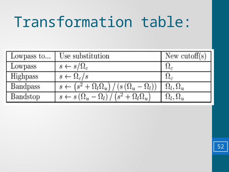
Transformation table:

52

Adaptive Digital Filters Top

9.6

• Adaptive digital filters are self learning filters, whereby an FIR (or IIR) is designed based on the characteristics of input signals. No other frequency response information or specification information is available.

• An adaptive digital filter is often represented by a signal flow graph with adaptive nature of weights shown:

x(k)Input

w0

x(k-1) x(k-2)

w1 w 2

AdaptiveWeights

d(k)

- +y(k)

Outpute(k)

Error

August 2007, Version 3.8/21/07 For Academic Use Only. All Rights Reserved

53

Adaptive Signal Processing: Top

9.7

“The aim is to adapt the digital filter such that the input signal x(k) is filtered to produce y(k) which when subtracted from desired signal d(k), will minimise the power of the error signal e(k).”

desiredsignal d(k)

input +y(k)signal

x(k)

Adaptive FIRDigital Filter Output-

signal

Adaptive Algorithm

e(k) = d(k) - y(k)

y(k) = Filter(x(k))

e(k)Σ

errorsignal

August 2007, Version 3.8/21/07 For Academic Use Only. All Rights Reserved

54

Adaptive Filter Nomenclature

• If the digital filter is FIR or all-zero, the adaptive system can also be called Moving Average or MA.

• If the digital filter is all-pole, the adaptive system can also be called Autoregressive or AR.

• If the digital filter is an IIR with zeros, the adaptive system can also be called ARMA.

• This presentation addresses FIR or MA filters only.

55

Coefficient Adaptation

• The principal behind determining the coefficients of the filter model is to maximize the statistical correlation between the desired signal and the coefficients.

• Typically, this is done by minimizing the correlation between the error signal and the filter state as is relevant to the coefficients.

• If the adaptive filter is working, the error signal decreases in magnitude, which slows down the movement of the coefficients. The filter is therefore converging to a solution. 56

Applications of Adaptive FiltersSystem identification: adaptive equalization

• The adaptive filter attempts to model an unknown external system.

Interference cancellation• The adaptive filter attempts to isolate the

component of a primary signal that is not part of a reference signal.

Linear prediction• This is like interference cancellation, but the

adaptive filter uses a delayed version of the primary signal as the reference.

57

Architectures

Delays(k) + n)k)

d(k)

Unknown x(k)

d(k)

y(k) +e(k)

Top

9.9

n’(k)x(k) Adaptive

Filter

y(k) +e(k)Σ s(k)-

Adaptive ΣSystem Filter -

Noise Cancellation

UnknownSystem

d(k)+

Inverse System Identification

d(k)

x(k) y(k) +e(k)x(k) AdaptiveFilter

y(k)Σ

-e(k) Delay

s(k)Adaptive Σ

Filter -

PredictionSystem Identification

August 2007, Version 3.8/21/07 For Academic Use Only. All Rights Reserved

58

Application Examples

• System Identification:

• Channel identification; Echo Cancellation

• Inverse System Identification:

• Digital communications equalisation.

• Noise Cancellation:

Top

9.10

• Active Noise Cancellation; Interference cancellation for CDMA

• Prediction:

• Periodic noise suppression; Periodic signal extraction;Speech coders; CMDA interference suppression.

August 2007, Version 3.8/21/07 For Academic Use Only. All Rights Reserved

59

Least-Mean-Square (LMS) Algorithm Linear adaptive filtering algorithm Differs from steepest descent Widely used for its simplicity

Consists of:1) A filtering process

(mainly FIR model)2) An adaptive process

60

Parameters: M = # of taps (length of filter) μ = step-size parameter

Filter output is: y(n) = ŵH(n)u(n)

Error signal is: e(n) = d(n) – y(n)

Tap-weight vector: ŵ(n+1) = ŵ(n) + μu(n)e*(n)

61

1. Let n=1

2. Compute the gain vector

3. Compute the true estimation error (n)

4. Update the estimate of the coefficient vector

5. Update the error correlation matrix

6. Increment n by 1, go back to step 2

ŵ(n) = ŵ(n-1) + k(n) (n)

p(n)= p(n-1)-k(n)uT(n)p(n-1)

k(n)= p(n-1)u(n)/1+uT(n) p(n-1)u(n)

Convergence is better but computationally expensive

The Recursive Least-Squares (RLS) Algorithm

62

Thank You

63