filtering turbulent systems with stochastic parameterized...

Filtering Turbulent Systems with StochasticParameterized “Extended” Kalman Filter

John Harlim

Department of MathematicsNorth Carolina State University

May 27, 2010

References:

a) Test Models for Improving Filtering with Model Errors through StochasticParameter Estimation (with B. Gershgorin and A.J. Majda), J. Comput.Phys., 229(1):1-31, 2010.

b) Improving Filtering and Prediction of Spatially Extended TurbulentSystems with Model Errors through Stochastic Parameter Estimation(with B. Gershgorin and A.J. Majda), J. Comput. Phys., 229(1):32-57,2010.

c) Filtering Turbulent Sparsely Observed Geophysical Flows (with A.J.Majda), Monthly Weather Review, 138(4): 1050-1083, 2010.

Review Article: Mathematical Strategies for Filtering Turbulent DynamicalSystems (with B. Gershgorin and A.J. Majda), DCDS-A: 27(2), 441-486, 2010.

Ch 13 of: Systematic Strategies for Real Time Filtering of Turbulent Signals inComplex Systems (with A.J. Majda), Cambridge University Press (inpreparation), 2010.

Online Model Error Estimation StrategyA simple strategy to cope with model errors for filtering with animperfect model nonlinear dynamical system depending onparameters, b,

du

dt= F (u, b)

is to augment the state variable u, by the parameters λ, and adjoinan approximate dynamical equation for the parameters

db

dt= g(b).

Online Model Error Estimation StrategyA simple strategy to cope with model errors for filtering with animperfect model nonlinear dynamical system depending onparameters, b,

du

dt= F (u, b)

is to augment the state variable u, by the parameters λ, and adjoinan approximate dynamical equation for the parameters

db

dt= g(b).

In hierarchical notation, filtering this augmented system is one wayof estimating

[u, b|v ] = [v |u, b] [u|b][b][v ]

The classical separate bias Kalman Filter

Friedland (1969, 1982) considered the following linear filteringproblem

um+1 = Fum + Bm+1bm+1 + σm+1

bm+1 = bm + σbm+1

with a biased observation model

vm+1 = Gum+1 + Cm+1bm+1 + σom+1

In this talk, we only consider unbiased observation, Cm = 0.

Constant bias model: bm+1 = bm

0 0.5 1 1.5 2 2.5 3 3.5 4 4.5 5−2

−1

0

1

2Qb=0, rmsb=0.47622, rms=0.44352

u

0 0.5 1 1.5 2 2.5 3 3.5 4 4.5 5−5

−4

−3

−2

−1

0

1

2

b

time

White noise bias model: bm+1 = bm + σbm+1

0 0.5 1 1.5 2 2.5 3 3.5 4 4.5 5−2

−1

0

1

2Qb=2, rmsb=0.53564, rms=0.34396

u

0 0.5 1 1.5 2 2.5 3 3.5 4 4.5 5−8

−6

−4

−2

0

2

4

b

time

Test model for true signal

Consider the following SDE

du(t)

dt= −γ(t)u(t) + iωu(t) + σW (t) + f (t)

as a test model for filtering with model error.



du(t)



To generate significant model errors as well as to mimicintermittent chaotic instability as often occurs in nature, we allowγ(t) to switch between stable (γ > 0) and unstable (γ < 0)regimes according to a two-state Markov jump process.



du(t)



To generate significant model errors as well as to mimicintermittent chaotic instability as often occurs in nature, we allowγ(t) to switch between stable (γ > 0) and unstable (γ < 0)regimes according to a two-state Markov jump process.Assume the following observation model:

vm = u(tm) + σom, σom ∼ N (0, ro). (1)

True Signals for Unforced and Forced cases

−1

−0.5

0

0.5

1R

e[u(

t)]

Unforced system

012

γ(t)

−1

0

1

Re[

u(t)

]

Forced system

0 50 100 150 200 250 300 350 400 450 500

012

t

γ(t)

Mean Stochastic Model

The prototype one-mode stochastic mean model

du(t) =[

(−γ + iω)u(t) + F (t)]

dt + σdW (t)

where one fits the parameters using climatological statisticalquantities such as the energy spectrum and correlation time.

Mean Stochastic Model

The prototype one-mode stochastic mean model

du(t) =[

(−γ + iω)u(t) + F (t)]

dt + σdW (t)

where one fits the parameters using climatological statisticalquantities such as the energy spectrum and correlation time.

This ”poor-man” strategy is discussed in Harlim and MajdaNonlinearity 2008, Comm. Math. Sci. 2010.

Stochastic Parameterized Extended Kalman Filter:

We consider the following canonical model that accounts additiveand multiplicative biases:

du(t) =[

(−γ(t) + iω)u(t) + F (t)+b(t)]

dt + σdW (t)

db(t) = (−γb + iωb)b(t)dt + σbdWb(t)

dγ(t) = −dγ(γ(t)− γ)dt + σγdWγ(t)



du(t) =[

(−γ(t) + iω)u(t) + F (t)+b(t)]

dt + σdW (t)



We find stochastic parameters {γb, ωb, σb, dγ , σγ} that are robustfor high filter skill beyond the MSM and in many occasionscomparable to the perfectly specified filter model.



du(t) =[

(−γ(t) + iω)u(t) + F (t)+b(t)]

dt + σdW (t)



We find stochastic parameters {γb, ωb, σb, dγ , σγ} that are robustfor high filter skill beyond the MSM and in many occasionscomparable to the perfectly specified filter model.

This special form has exactly solvable nonlinear solutions andmoments and we do not need any linearization as in the standardEKF.

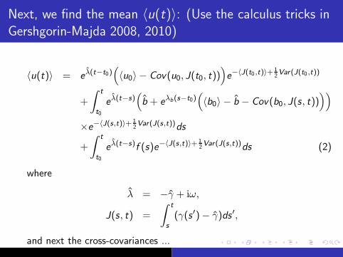
Next, we find the mean 〈u(t)〉: (Use the calculus tricks in

Gershgorin-Majda 2008, 2010)

〈u(t)〉 = eλ(t−t0)(

〈u0〉 − Cov(u0, J(t0, t)))

e−〈J(t0 ,t)〉+12Var(J(t0 ,t))

+

∫ t

t0

eλ(t−s)(

b + eλb(s−t0)(

〈b0〉 − b − Cov(b0, J(s, t))))

×e−〈J(s,t)〉+ 12Var(J(s,t))ds

+

∫ t

t0

eλ(t−s)f (s)e−〈J(s,t)〉+ 12Var(J(s,t))ds (2)

where

λ = −γ + iω,

J(s, t) =

∫ t

s

(γ(s ′)− γ)ds ′,

and next the cross-covariances ...

SPEKF: Checking first and second ordered statistics

1.8 2 2.2 2.4 2.6

−1

−0.5

0

t

<Re[u]>

1.8 2 2.2 2.4 2.6

1

1.2

1.4

t

Var(u)

1.8 2 2.2 2.4 2.6

−0.8−0.6−0.4−0.2

00.2

t

<Re[Cov(u,u*)]>

1.8 2 2.2 2.4 2.6

−0.1

0

0.1

t

<Re[Cov(u,γ)]>

1.8 2 2.2 2.4 2.60.4

0.5

0.6

0.7

t

<Re[Cov(u,b)]>

1.8 2 2.2 2.4 2.6

−0.4

−0.3

−0.2

−0.1

0

0.1

t

<Re[Cov(u,b*)]>

One mode demonstration of the filtered solution:

observed mode

70 75 80 85 90 95 100−1.5

−1

−0.5

0

0.5

1

1.5∆ t=0.25, ro=E=0.008, perfect model, RMS x=0.042

x

true signalobservationposterior mean

70 75 80 85 90 95 100−1.5

−1

−0.5

0

0.5

1

1.5NEKF-C: dγ =0.01d, σγ =5σ , γb =0.1d, σb =5σ , RMS x=0.052

x

70 75 80 85 90 95 100−1.5

−1

−0.5

0

0.5

1

1.5MSM: RMS x= 0.14

x

time

One mode demonstration of the filtered solution:

unobserved parameters

70 75 80 85 90 95 100−3

−2.5

−2

−1.5

−1

−0.5

0

0.5

1

1.5

2NEKF-C: dγ =0.01d, σ γ =5σ , γb =0.1d, σ b =5σ

Rea

l[b]

70 75 80 85 90 95 100−0.5

0

0.5

1

1.5

2

2.5

3

3.5NEKF-C: dγ =0.01d, σ γ =5σ , γb =0.1d, σ b =5σ , RMS γ=0.7

γ

true signalposterior mean

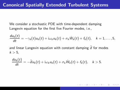
Canonical Spatially Extended Turbulent Systems

We consider a stochastic PDE with time-dependent dampingLangevin equation for the first five Fourier modes, i.e.,

duk(t)

dt= −γk(t)uk(t) + iωkuk(t) + σkWk(t) + fk(t), k = 1, . . . , 5,

and linear Langevin equation with constant damping d for modesk > 5,

duk(t)

dt= −duk(t) + iωkuk(t) + σkWk(t) + fk(t), k > 5.

Turbulent barotropic Rossby wave equation:

ωk = −β/k ,Ek = k−3

(a)

240 245 250 255 260 265 2700

1

2

3

4

5

6

240 245 250 255 260 265 270−0.5

0

0.5

1

1.5

2

2.5(b)

Incorrectly specified forcings:

Here, we consider a true signal with forcing given by

fk(t) = Af ,k exp(

i(ωf ,kt + φf ,k))

, (3)

for k = 1, . . . , 7 with amplitude Af ,k , frequency ωf ,k , and phaseφf ,k drawn randomly from uniform distributions,

Af ,k ∼ U(0.6, 1),

ωf ,k ∼ U(0.1, 0.4),

φf ,k ∼ U(0, 2π),

fk = f ∗−k ,

and unforced, fk(t) = 0, for modes k > 7. However, we do notspecify this true forcing to the filter model, i.e., we use fk = 0 forall modes.

Reduced Filter Domain Kalman Filter for regularly

spaced sparse observation

We consider regularly spaced sparse observations: (2M + 1)observations of (2N + 1) model grid points. The Fouriercoefficients of the observation model is given as

vℓ,m =∑

k∈A(ℓ)

uk,m + σom,

where

A(ℓ) = {k |k = ℓ+ (2M + 1)q, q ∈ Z, |ℓ| ≤ N}is the aliasing set of wavenumber ℓ. (Majda-Grote PNAS 2007)

Reduced Filter Domain Kalman Filter for regularly

spaced sparse observation

We consider regularly spaced sparse observations: (2M + 1)observations of (2N + 1) model grid points. The Fouriercoefficients of the observation model is given as

vℓ,m =∑

k∈A(ℓ)

uk,m + σom,

where

A(ℓ) = {k |k = ℓ+ (2M + 1)q, q ∈ Z, |ℓ| ≤ N}is the aliasing set of wavenumber ℓ. (Majda-Grote PNAS 2007)

When the energy spectrum is decaying as a function of k , we canuse the following reduced observation model

v ′ℓ,m ≡ vℓ,m −∑

k∈A(ℓ),k 6=ℓ

uk,m|m−1 = uℓ,m + σom.

Example: 123 grid pts (61 modes) but only 41 observations (20modes) available

sparse observations for P=3

Physical Space

Fourier Space

0 20-20 61-61

aliasing set !(1) = {1,-40,42} for P=3 and M=20

0 20-20 61-61

aliasing set !(11) = {11,-30,52} for P=3 and M=20

Incorrectly specified forcings, observed only 15

observations of 105 grid points

1 2 3 4 5 1010−4

10−3

10−2

10−1

100

k

Ene

rgy

Spe

ctru

m

(b)

1 2 3 4 5 6 7 8 9

0.05

0.1

0.15

0.2

0.25

0.3

0.35

0.4

0.45

RM

S E

rror

k

(a)

natureNEKFperfectCSM fCSMobs

Table of RMSE for the SPDE test case with

intermittent burst of instability

Forcing unforced case correct forcing incorrect forcing

ro 0.2 0.3 0.5

perfect filter 0.35 0.39 0.45MSM 0.39 0.48 0.73

MSMf=0 - - 1.17

SPEKF-C 0.38 0.44 0.59SPEKF-M 0.36 0.42 0.79SPEKF-A 0.39 0.46 0.60

Canonical Model for Midlatitude Geophysical Flows:

The dynamical equations for the perturbed variables are:

∂q1∂t

+ J(ψ1, q1) + U∂q1∂x

+ (β + k2dU)∂ψ1

∂x+ ν∇8q1 = 0

∂q2∂t

+ J(ψ2, q2)− U∂q2∂x

+ (β − k2dU)∂ψ2

∂x+ ν∇8q2 + κ∇2ψ2 = 0

where qj is the quasi-geostrophic potential vorticity given as

qj = βy +∇2ψj +k2d2(ψ3−j − ψj )

with ~u = ∇⊥ψ, kd =√8/Ld .

In the two-layer case, the barotropic vertical and baroclinic modesare defined as ψb = (ψ1 + ψ2)/2 and ψc = (ψ1 − ψ2)/2,respectively.

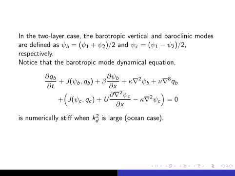
In the two-layer case, the barotropic vertical and baroclinic modesare defined as ψb = (ψ1 + ψ2)/2 and ψc = (ψ1 − ψ2)/2,respectively.Notice that the barotropic mode dynamical equation,

∂qb∂t

+ J(ψb , qb) + β∂ψb

∂x+ κ∇2ψb + ν∇8qb

+(

J(ψc , qc) + U∂∇2ψc

∂x− κ∇2ψc

)

= 0

is numerically stiff when k2d is large (ocean case).

The 2-layer QG model with baroclinic instability

1 2 3 4 5 6

1

2

3

4

5

6

−1 −1−0.8

−0.8

−0.8

−0.6

−0.6

−0.6 −0.6

−0.4

−0.4 −0.4−0.2 −0.2

−0.2

−0.2

0 0

0

0

0.2 0.2

0.2

0.2

0.4 0.4

0.40.4

0.6 0.6

0.60.6

0.8 0.8

0.8

0.8

1

1

X

Y

ATM REGIME F=4 AT TIME=2500

1 2 3 4 5 6

1

2

3

4

5

6

−1

−1

−0.8

−0.8

−0.6

−0.6

−0.6

−0.6

−0.4−0.4

−0.4−0.4

−0.2−0.2

−0.2−0.2

0

0

0

00

0.2

0.2

0.20.2

0.4

0.4

0.40.4

0.6

0.6

0.6

0.8

0.8

0.81

1

X

Y

ATM REGIME F=4 AT TIME=5000

1 2 3 4 5 6

1

2

3

4

5

6−1

−1

−1

−1

−0.8

−0.8

−0.8

−0.6

−0.6

−0.6

−0.4

−0.4

−0.4

−0.2

−0.2

−0.2

0

0

0

0

0.2

0.2

0.2

0.4

0.4

0.4

0.6

0.6

0.6

0.8

0.8

0.8

1

1

1

1

X

Y

OCN REGIME F=40 AT TIME=100

1 2 3 4 5 6

1

2

3

4

5

6

−1

−1

−1

−1

−0.8

−0.8

−0.8

−0.8

−0.6

−0.6

−0.6

−0.6

−0.4

−0.4

−0.4

−0.4

−0.2

−0.2

−0.2

−0.2

0

0

0

0

0.2

0.2

0.2

0.2

0.4

0.4

0.4

0.4

0.6

0.6

0.6

0.6

0.8

0.8

0.8

0.8

1

1

1

1

X

Y

OCN REGIME F=40 AT TIME=200

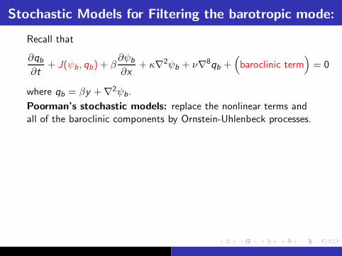
Stochastic Models for Filtering the barotropic mode:

Recall that

∂qb∂t


∂x+ κ∇2ψb + ν∇8qb +

(

baroclinic term)

= 0

where qb = βy +∇2ψb.


Recall that

∂qb∂t


∂x+ κ∇2ψb + ν∇8qb +

(

baroclinic term)

= 0


Poorman’s stochastic models: replace the nonlinear terms andall of the baroclinic components by Ornstein-Uhlenbeck processes.


Recall that

∂qb∂t


∂x+ κ∇2ψb + ν∇8qb +

(

baroclinic term)

= 0


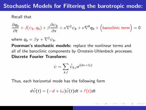
Poorman’s stochastic models: replace the nonlinear terms andall of the baroclinic components by Ornstein-Uhlenbeck processes.Discrete Fourier Transform:

ψ =∑

k,ℓ

ψk,ℓei(kx+ℓy)

Thus, each horizontal mode has the following form

d ψ(t) = (−d + iω)ψ(t)dt + f (t)dt


Recall that

∂qb∂t


∂x+ κ∇2ψb + ν∇8qb +

(

baroclinic term)

= 0


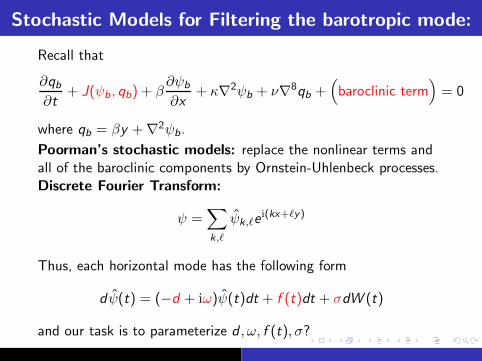
Poorman’s stochastic models: replace the nonlinear terms andall of the baroclinic components by Ornstein-Uhlenbeck processes.Discrete Fourier Transform:

ψ =∑

k,ℓ

ψk,ℓei(kx+ℓy)

Thus, each horizontal mode has the following form

d ψ(t) = (−d + iω)ψ(t)dt + f (t)dt + σdW (t)

and our task is to parameterize d , ω, f (t), σ?

Statistical Quantities: Climatological variances of

the barotropic mode

100 101 102 103 1040

0.1

0.2

0.3

0.4

0.5

0.6

0.7

Rel

ativ

e V

aria

nce

in %

mode

atm (F=4)ocn (F=40)atm (F=4) with stronger bottom drag

“Atmospheric” case (k2d is small) and “oceanic” case (k2d is large).

Statistical Quantities: Histogram “marginal pdf’s”

Statistical Quantities: Correlation functions

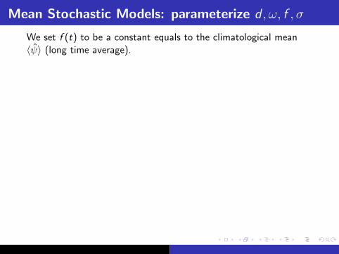
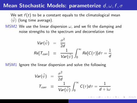
Mean Stochastic Models: parameterize d , ω, f , σ

We set f (t) to be a constant equals to the climatological mean〈ψ〉 (long time average).



MSM2 We use the linear dispersion ω, and we fit the damping andnoise strengths to the spectrum and decorrelation time

Var(ψ) =σ2

2d

Re[Tcorr ] ≡ 1

Var(ψ)

∫ ∞

0Re[C (τ)]dτ =

1

d



MSM2 We use the linear dispersion ω, and we fit the damping andnoise strengths to the spectrum and decorrelation time

Var(ψ) =σ2

2d

Re[Tcorr ] ≡ 1

Var(ψ)

∫ ∞

0Re[C (τ)]dτ =

1

d

MSM1 Ignore the linear dispersion and solve the following

Var(ψ) =σ2

2d

Tcorr ≡ 1

Var(ψ)

∫ ∞

0C (τ)dτ =

1

d + iω

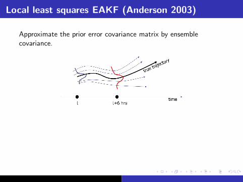
Local least squares EAKF (Anderson 2003)

Approximate the prior error covariance matrix by ensemblecovariance.



How many ensemble member? How to avoid ensemble collapseand spurious correlations due to finite ensemble size?



How many ensemble member? How to avoid ensemble collapseand spurious correlations due to finite ensemble size?Computationally, EAKF requires extensive tunings of ensemblesize, local box size, covariance inflation, and in the ocean case,integration time step need to be reduced.

Longer deformation radius case (“atmospheric”

regime).

0 100 200 300 400 500 600 700 800 900 10000

0.1

0.2

0.3

0.4

0.5

0.6

RM

S

36OBS F=4, Tobs=0.25, ro=0.17113, K=48, r=0.2, L=14

NEKFMSM1MSM2LLS−EAKFobs error

1 2 3 4 5 6 7 8 9 10 11 1210−4

10−2

100

102

Spe

ctra

mode

NEKFMSM1MSM2trueLLS−EAKF

Shorter deformation radius case (“oceanic” regime).

0 20 40 60 80 100 120 140 160 180 2000

2

4

6

8

10

12

14

16

18

RM

S

36 OBS F=40, Tobs=0.02, ro=17.3655, K=48, r=0.2, L=14

SPEKFMSM1MSM2LLS−EAKFobs error

1 2 3 4 5 6 7 8 9 10 11 1210−4

10−2

100

102

Spe

ctra

mode

SPEKFMSM1MSM2trueLLS−EAKF

1 2 3 4 5

1

2

3

4

5

−1

−1 −1

−0.

8

−0.8 −0.8

−0.6

−0.6

−0.6

−0.4

−0.4

−0.4

−0.

2

−0.2

−0.2

0

0

0

0

0.2

0.2

0.2

0.4

0.4

0.4

0.6

0.6

0.6

0.8

0.8

0.8

1

1

1

1

TRUE AT T=100

1 2 3 4 5

1

2

3

4

5 −1

−1

−0.8

−0.8

−0.6

−0.6

−0.4

−0.4

−0.4

−0.4

−0.2

−0.2−

0.2

0

0

0

0

0.2

0.2

0.2

0.4

0.4

0.40.6

0.8

1

1

LLS−EAKF, Tobs=0.02, RO=17.3655

1 2 3 4 5

1

2

3

4

5

−1

−1

−1

−0.

8

−0.8

−0.6

−0.6

−0.4

−0.4

−0.2

−0.2

0

0

0

0.2

0.2

0.2

0.4

0.4 0.4

0.6

0.6

0.6

0.8

0.8

0.8

1

1

1

1

SPEKF, Tobs=0.02, RO=17.3655

1 2 3 4 5

1

2

3

4

5

−1

−1

−1

−0.8

−0.8

−0.6

−0.6

−0.

4

−0.4

−0.

2

−0.2

0

0

0 0

0.2

0.2

0.2

0.4

0.4

0.4

0.6

0.6

0.6

0.8

0.8

0.8

1

1

1

OBS, Tobs=0.02, RO=17.3655

Summary:

1. MSM: We introduce reduced stochastic models throughreplacing the nonlinearity and baroclinic components withOrnstein-Uhlenbeck process for filtering purpose. Thisreduced poor man’s strategy is numerically very cheap andaccurate in a regime when the dynamical systems is stronglychaotic and fully turbulent.

Summary:

1. MSM: We introduce reduced stochastic models throughreplacing the nonlinearity and baroclinic components withOrnstein-Uhlenbeck process for filtering purpose. Thisreduced poor man’s strategy is numerically very cheap andaccurate in a regime when the dynamical systems is stronglychaotic and fully turbulent.

2. SPEKF: We introduce a paradigm model for “online” learningboth the additive and multiplicative biases from observationsbeyond the MSM. This model is analytically solvable suchthat NO LINEARIZATION is needed when Kalman filterformula is utilized.

filtering turbulent systems with stochastic parameterized...

Documents