fieldwork investigating the offshore queen charlotte ... · system in southeastern alaska, and its...

U.S. Department of the InteriorU.S. Geological Survey

Fieldwork

http://soundwaves.usgs.gov/

Sound Waves Volume FY 2015–2016, Issue No. 160 December 2015–January 2016

Southeastern Alaska and the adjacent part of northwestern Canada form an important part of the boundary between the Pacific and North American tectonic plates. This region contains a fault system that is like California’s San Andreas fault: the tectonic plates move past each other horizontally at a rate of approximately 50 millimeters/year along the southeastern Alaska coastline. Like the San Andreas fault, the Queen Charlotte-Fairweather fault is right-lateral: to an observer on one side of the fault, the block on the other side is moving to the right.

Along the southern part of this fault margin, the plate boundary is fairly simple, with the right-lateral Queen Charlotte-Fairweather fault accommodating most of the relative motion between the two tectonic plates. In the region northwest of Glacier Bay National Park, however, the distribution of relative motion is not well understood. Relative plate motion in southeastern Alaska appears to be partitioned among several faults, most of which are located offshore. Understanding the partitioning of motion between onshore and offshore faults remains a major scientific problem, as it has significant implications for earthquake hazards throughout the region. If the motion is on one fault, then the hazard is confined to that fault, but if the motion is distributed across several faults over a broad width, then the region of earthquake hazard can be larger.

Investigating the Offshore Queen Charlotte-Fairweather Fault System in Southeastern Alaska, and its Potential to Produce Earthquakes, Tsunamis, and Submarine Landslides By Danny Brothers, Jamie Conrad, Peter Haeussler, Pete Dartnell, and Katie Maier

Lituya Bay

Craig

Haida Gwaii

Gulf of Alaska

Mount Crillon

QCFF

Cape Felix

Mount Fairweather

QCFF

Overview map of study region along the Queen Charlotte-Fairweather fault offshore southeastern Alaska. Black rectangles (Survey Areas 1 and 2) show locations of two USGS-led marine geophysi-cal surveys carried out in May and August 2015. A third, Canadian-led cruise conducted seafloor surveying and sampling offshore Haida Gwaii, British Columbia, and southernmost Alaska in Sep-tember 2015 (see inset map). Details of Survey Area 1 are shown in enlarged map on page 3. CSF, Chatham Strait fault; CSZ, Coastal shear zone; LIPSF, Lisianski Inlet-Peril Strait fault; QCFF, Queen Charlotte-Fairweather fault.

(Alaska Fault System continued on page 2)

2December 2015–January 2016 Sound Waves Fieldwork

Contents

Fieldwork 1Spotlight on Sandy 12Outreach 16Meetings 18Publications 19

Sound Waves

Editor Jolene Gittens

St. Petersburg, Florida Telephone: 727-502-8038

E-mail: [email protected] Fax: 727-502-8182

Print Layout Editor Betsy Boynton


E-mail: [email protected] Fax: 727-502-8182

Web Layout Editor Betsy Boynton


E-mail: [email protected] Fax: (727) 502-8182

SOUND WAVES (WITH ADDITIONAL LINKS) IS AVAILABLE ONLINE AT URL http://soundwaves.usgs.gov/

Submission Guidelines

Deadline: The deadline for news items and publication lists for the February/March issue of Sound Waves is Tuesday, February 16, 2016.Publications: When new publications or products are released, please notify the editor with a full reference and a bulleted summary or description.Images: Please submit all images at publica-tion size (column, 2-column, or page width). Resolution of 200 to 300 dpi (dots per inch) is best. Adobe Illustrator© files or EPS files work well with vector files (such as graphs or diagrams). TIFF and JPEG files work well with raster files (photographs or rasterized vec-tor files).Any use of trade, firm, or product names is for descriptive purposes only and does not imply endorsement by the U.S. Government.

U.S. Geological Survey Earth Science Information Sources:

Need to find natural-science data or information? Visit the USGS Frequently Asked Questions (FAQ’s) at URL http://www.usgs.gov/faq/Can’t find the answer to your question on the Web? Call 1-888-ASK-USGSWant to e-mail your question to the USGS? Send it to this address: [email protected]

In 2012 and 2013, a series of large-magnitude earthquakes and associated aftershocks occurred along the south-ern section of the Queen Charlotte-Fairweather fault system. The first was a magnitude 7.8 thrust-fault earthquake near Haida Gwaii—a group of islands offshore British Columbia near the south end of the Queen Charlotte-Fairweather fault. Just south of this area, the Juan de Fuca plate is subducting (pushing beneath) the North American plate. Com-pression near a subduction zone com-monly produces thrust faulting, in which rock on one side of the fault moves up and over rock on the other side. This earthquake led to tsunami warnings and evacuations in Canada, Alaska, Wash-ington, Oregon, California, and Hawai'i. The second earthquake, magnitude 7.5, was generated by strike-slip faulting (where rock on one side of the fault moves sideways past rock on the other

(Alaska Fault System continued from page 1)

Survey team on fantail of research vessel (R/V) Solstice posing between the multichannel seis-mic-reflection streamer (green coil) and multibeam bathymetry sonar (out of view, attached to horizontal pole on left side of photo). Standing, left to right: James Weise (Alaska Department of Fish and Game [ADFG]), Pete Dartnell (USGS), Dave Anderson (ADFG), Rob Wyland (USGS), John Crowfts (ADFG), and Peter Haeussler (USGS). Kneeling, left to right: Danny Brothers (USGS) and Gerry Hatcher (USGS). The multibeam sonar sends and receives sound energy that bounces off the seafloor and provides information used to calculate seafloor depths. The streamer contains hydro-phones (underwater microphones) that receive sound energy reflected from layers of sediment beneath the seafloor, used to produce cross-sectional images of the layers.

Earthquakes Prompt Marine Hazards In-vestigation

During the last century, the Queen Charlotte-Fairweather fault system has generated six magnitude 7 or greater earthquakes, including a magnitude 8.1 in 1949 offshore British Columbia—Canada’s largest recorded earthquake. A magnitude 7.8 earthquake in 1958 triggered a landslide in Lituya Bay, Alaska, and generated the largest tsunami run-up ever recorded (524 meters/1,720 feet up a mountainside). At risk are the growing populations of Juneau (Alaska’s state capital), Sitka, and other communities throughout southeastern Alaska. Additionally, more than 1 million tourists are drawn to view and explore the region’s natural wonders each year, making many people vulnerable to its earthquake and tsunami hazards. Also at risk are sea-bottom cables that cross the fault system and are critical to the state’s communications.


Fieldwork, continued

http://www.usgs.gov/faq/

http://www.usgs.gov/faq/

mailto:[email protected]

3 Sound Waves December 2015–January 2016


Fieldwork

Preliminary results have provided unprece-dented imagery of the fault shape and struc-ture, deformation history, and sedimentary processes in the area just offshore Glacier Bay National Park (see enlarged maps, below). The scientists presented many of their findings, maps, and images in a poster

session at the American Geophysical Union Fall Meeting in December 2015 (<https://agu.confex.com/agu/fm15/meetingapp.cgi/Paper/68335>). Ongoing analysis and comparison with older data are expected to yield additional insights.


El�n CoveEl�n Cove

25 12.5 0 km

A

B

Left: Enlarged map of Study Area 1, showing new multibeam bathymetry data (rainbow colors) ac-quired on the R/V Solstice near Cross Sound and Glacier Bay National Park, southeastern Alaska. Red arrows highlight the surface expression, or trace, of the Queen Charlotte-Fairweather fault. Red rectangle is area of expanded map, right, showing en echelon basins along the fault and right-lateral offset of the south wall of the Yakobi Sea Valley. Line A–B on expanded map shows location of multichannel seismic-reflection profile, top of page 4.

Stunning Images of a Seafloor FaultDanny Brothers’ love for revealing Earth’s unseen surfaces is apparent—he’s spent more than 450 days on the water imaging

underwater features off the U.S east coast, much of California, and southern Alaska, as well as in the Salton Sea and Lake Tahoe. While Brothers has terrestrial passions, such as mountain biking, nothing makes him smile like discovering the perfect trace of a strike-slip fault on the seafloor. When he and his fellow mappers were bobbing above the 825-mile-long Queen Charlotte-Fairweather fault, one of the fastest-moving strike-slip faults in the world, they had only a faint idea of how the new, high-resolution imagery would look as USGS instruments beamed it back to the boat. It was the first time anyone had used modern technology to map this piece of seafloor off southeastern Alaska. “What we saw was the most stunning morphological expression of a strike-slip fault I had ever seen,” said Brothers, describing the quintessential fault cutting straight across the seafloor, offsetting seabed channels and submerged glacial valleys, the evidence all perfectly preserved since the last ice age. It was an unusual opportunity to observe how a fault has evolved in 20,000 years, he explained, because rivers and glaciers obliterate much of the record on land. It was clear to Brothers that undersea work off Alaska’s shores was essential to truly comprehend the natural hazards facing southeastern Alaska. This discovery also opened up future research possibilities—quite literally—because the scientists found that the moving fault had created scarps, or fresh surfaces, that animals, such as corals, could colonize. Now it’s likely that remotely operated vehicles and camera sleds will soon be added to the mapping team’s quiver of cutting-edge underwater tools. —Amy West

side, typical of the right lateral Queen Charlotte-Fairweather fault). It occurred farther north in U.S. territory, west of the town of Craig, Alaska. These two earthquakes triggered significant concern from the Earth sciences community and led to a general realization that, because of its offshore location, relatively little is known about the Queen Charlotte-Fair-weather fault system and the geohazards associated with it.

In 2015, marine-geohazards researchers at the U.S. Geological Survey (USGS) teamed up with scientists from the Alaska Department of Fish and Game and the Geological Survey of Canada to begin the first phase of a multiyear, onshore-offshore study of the Queen Charlotte-Fairweather fault system. The overarching goal of the study is to better understand the earthquake, tsunami, and submarine-landslide hazards throughout southeastern Alaska and to develop geological models that can be applied to other major strike-slip plate boundaries around the globe, such as the San Andreas fault system of California, the Alpine fault of New Zealand, and the North Anatolian fault of Turkey.

Research cruises conducted in May, August, and September 2015 represent the first systematic efforts to study the offshore Queen Charlotte-Fairweather fault system in U.S. territory in more than three decades.


4December 2015–January 2016 Sound Waves


Fieldwork

First Cruise: Imaging the Seafloor and Lay-ers Beneath the Seafloor

The first phase of fieldwork began in May 2015, with a three-week cruise on the Alaska Department of Fish and Game research vessel (R/V) Solstice to collect marine geophysical data. These included bathymetric data (seafloor depths) and seis-mic-reflection data (cross-sectional images of sedimentary layers and other features beneath the seafloor). A team of USGS sci-entists—Danny Brothers, Pete Dartnell, Gerry Hatcher, and Rob Wyland from the Pacific Coastal and Marine Science Center and Peter Haeussler from the Alaska Science Center (see photo, page 2)—led multibeam bathymetry and mul-tichannel seismic-reflection surveys along the northernmost offshore section of the Queen Charlotte-Fairweather fault, between Cross Sound and Icy Point (see lefthand map, page 3). North of the survey area, the Queen Charlotte-Fairweather fault takes a westerly bend, producing some shorten-ing between the two plates. The 3,879 meter/12,726-foot-tall, ice-covered Mount Crillon and 4,671 meter /15,325-foot-tall Mount Fairweather are striking examples of the tectonic uplift resulting from that shortening.

During the May 2015 cruise, the team conducted surveys for one to two days, then anchored to catch up on data processing (and sleep) in nearby fjords along the western boundary of Glacier Bay National Park. After 17 days in the study area, the team acquired approximately 650 square kilometers of high-resolution multibeam bathymetry and more than 2,000 kilometers of multichannel seismic-reflection profiles, revealing a textbook example of strike-slip fault morphology (see enlarged map on left, page 3; with detail area shown on right) and evidence for post-glacial (approximately 19,000 years to present) fault movement.

Second Cruise: Looking for Fault Offset and Recent Earthquake Evidence

During a second cruise in early August, Danny Brothers, Jamie Conrad, and Jackson Currie of the Pacific Coastal and Marine Science Center joined Peter Haeussler and Greg Snedgen of the Alaska Science Center on the USGS R/V

Alaskan Gyre to achieve two primary objectives: • Target evidence for Holocene (less than

approximately12,000-year-old) faultoffset in the vicinity of Cross Soundby collecting chirp subbottom profiles.These are similar to multichannel seis-mic-reflection profiles but are producedwith higher-frequency sound energyand so provide much greater detail,although they do not extend as deepbeneath the seafloor.

• Identify geologic evidence for recentearthquakes along the Chatham StraitFault and the Coastal Shear Zone (see“Survey Area 2” in overview map).

The team ended up with more more than 250 kilometers of chirp subbottom data and roughly 150 kilometers of multichan-nel seismic-reflection data.

Throughout the summer and fall, scien-tists at the Pacific Coastal and Marine Sci-ence Center in Santa Cruz, California (Pete Dartnell, Jared Kluesner, Pat Hart, Alicia Balster-Gee, and Danny Brothers), have been diligently working through the data analysis, including the development of some new, advanced approaches to seismic-reflection data processing. Ini-tial results are phenomenal, showing the Queen Charlotte-Fairweather fault as a nearly straight seafloor lineament for more than 75 kilometers in the bathymetric data. Tears along the fault trace have resulted in a series of small en echelon fault basins

and the horizontal offset of seabed features (see enlarged maps, page 3).

Third Cruise: Sampling the Seafloor near British Columbia

Colleagues at the Geological Survey of Canada (Vaughn Barrie) and the Sitka Sound Science Center (Gary Greene; also emeritus faculty at Moss Landing Ma-rine Labs), led a third cruise, which was

Queen Charlotte-Fairweather fault

A B


Multichannel seismic-reflection profile shows sediment layers beneath the seafloor disrupted by the Queen Charlotte-Fairweather fault. The data were collected near Cross Sound, along line A–B on expanded bathymetric map, above. The profile is approximately 16 kilometers across, and it extends approximately 370 meters beneath the seafloor at the site of the Queen Charlotte-Fairweather fault.

Piston core recovery aboard the Canadian Coast Guard vessel John P. Tully. Gary Greene (left, Sitka Sound Science Center), Kim Conway (middle, Geological Survey of Canada), and Katie Maier (right, USGS) remove a plastic core liner full of seabed sediment from the core barrel (orange, in background). This core sampled a location near the Queen Charlotte-Fairweather fault offshore southern Alaska.




Fieldwork

funded by the USGS Earthquake Hazards Program and included USGS participants Jamie Conrad and Katie Maier of the Pacific Coastal and Marine Science Center. Conducted in September 2015 aboard the Canadian Coast Guard vessel John P. Tully, this cruise surveyed several areas along the southern part of the Queen Charlotte-Fairweather fault offshore Haida Gwaii, British Columbia, and southernmost Alaska. The crew used a chirp subbottom profiler and a deep-water camera system to pick sea-floor areas near the fault for sampling with a 20-foot-long piston corer. They recovered sediment cores as long as 14 feet. Sediment from these cores will be analyzed to provide age data that will help determine information about fault displacements (how far places on either side of the fault have moved rela-tive to each other) and ages of deformation. In addition, a nearshore area off Cape Felix, Alaska, was investigated for possible fault splays (subsidiary faults that branch from the main fault) extending north from the Queen Charlotte-Fairweather fault into the Alexan-der Archipelago—the islands that make up much of southeastern Alaska.

One surprising result from this cruise was the discovery of a 250-meter-high volcano-like cone at a depth of about 1,250 meters, about 10 kilometers west of the Queen Charlotte-Fairweather fault. On

top of this cone was an active fluid plume, which could be seen on sonar records to be rising 700 meters up into the water column. The deep-water camera system revealed abundant evidence of fluids emanating from the mound, including likely vents, formation of authigenic (precipitated in place) carbonate, and chemosynthetic biological communities, which use components of the fluids (such as hydrogen sulfide or methane) as primary energy sources rather than light. The mound was sampled with a grab sampler to collect pieces of the carbonate and unusual biota for further study. (See “Active Mud Volcano Field Discovered off Southeast Alaska,” in Eos, <https://eos.org/articles/active-mud-volcano-field-discovered-off-southeast-alaska>.)

Onshore Photographic and Lidar DataData from the cruises will be combined

with new results from fieldwork led by Rob Witter and Peter Haeussler of the Alaska Science Center, Kate Scharer of the USGS Earthquake Hazards Program field office in Pasadena, California, and Chris DuRoss of the USGS Geologic Hazards Science Center in Golden, Colorado. Airborne pho-tography and lidar missions were flown in late August over the onshore section of the Queen Charlotte-Fairweather fault along the western edge of Glacier Bay National

Park. Lidar is a remote-sensing technology that uses laser light to make precise mea-surements of elevation. Combining the on-shore lidar data with the seafloor bathymet-ric data will provide nearly seamless data coverage connecting the onshore topogra-phy and offshore bathymetry and allowing us to study this particular section of the Queen Charlotte-Fairweather fault across a wide range of spatial and temporal scales over contrasting geological environments. The lidar data will be used for on-land fault mapping and targeted paleoseismic inves-tigations (studies of evidence for ancient earthquakes) in the summer of 2016.

Also scheduled for 2016 is the begin-ning of an expanded, comprehensive study of the Queen Charlotte-Fairweather fault system for which the USGS Coastal and Marine Geology Program is currently preparing. The team of scientists from the Pacific Coastal and Marine Science Center and the Alaska Science Center will join forces with Uri ten Brink, Jason Chaytor, and Nathan Miller of the USGS Woods Hole Coastal and Marine Science Center in Woods Hole, Massachusetts. Plans are in the works for a sequence of marine geophysical and geological surveys—stayed tuned!

For more information, please contact Danny Brothers, [email protected].

Left: Profile of newly discovered volcano-like cone in sonar record collected off southernmost Alaska. Note fluid plume (blue) rising more than 700 meters upward from the top of the cone. Right: Further evidence of fluid venting from the cone includes these clams (Calyptogena spp.), which live on nutrients produced by chemosynthetic bacteria that use components of the fluid (such as hydrogen sulfide or methane) as primary energy sources.




Fieldwork

bubbles in the ice. The USGS research-ers were particularly interested in another strong radio-wave reflector: the interface between freshwater and saltwater. They

(Eroding Bluffs continued on page 7)

An Inside Look at Eroding Coastal Bluffs on Alaska’s North SlopeBy Peter Swarzenski and Bruce Richmond

In September 2015, scientists from the U.S. Geological Survey (USGS) and the University of California, Santa Cruz (UCSC) surveyed rapidly eroding perma-frost bluffs on Barter Island, a remnant of low-elevation tundra on Alaska’s Arctic coast. Warming air and sea temperatures in the Arctic are leading to longer periods of permafrost thaw and ice-free condi-tions during the summer months, which can weaken the coastal bluffs and increase their vulnerability to storm surge and wave impacts. The 2015 survey is part of a long-term effort to document seasonal to decadal coastal-bluff change on the island’s north coast.

In spite of bleak weather conditions that thwarted scheduled flights to Barter Island for many days, the survey team achieved its goals on the island. The researchers drilled into the permafrost to obtain samples of permafrost ice, pore water, and sediment. They are using geochemical techniques, such as measurement of radon and stable isotopes, to trace the movement of ground-water and examine its effects on sediment erosion. Several geophysical techniques were used to image the subsurface structure of permafrost features, such as ice-wedge polygons, and to measure the salt content and internal structure of materials that make up the frozen ground.

Repeat electrical resistivity tomograms (ERTs) had been collected on the coastal bluffs in Barter Island in early and late summer 2014 to evaluate the effects of one summer’s thaw cycle. ERTs provide a cross-sectional view of electrical resistiv-ity within the bluffs. Because ice is a poor conductor of electricity and thus has high resistivity, ERTs reveal the distribution of subsurface permafrost. ERTs were collected from the same bluffs during the 2015 sur-vey to examine annual change and to iden-tify sites for drilling into the permafrost.

To complement these geo-electrical methods, the September 2015 survey team collected data with a phase-sensitive radio echo sounder (pRES). Whereas traditional echo sounders send sound waves through water to detect boundaries between materials with differing physical

143°35'W143°40'W143°45'W

70°8

'N70

°7'N

70°6

'N

1 KILOMETER

1 MILE

EXPLANATIONElevation (meters)

High : 15

Low : 0

1 KILOMETER

1 MILE

Bernard Spit

Kaktovik

Existing airstrip

LRRS

New airstrip KaktovikLagoon

Beaufort Sea

AreyLagoon

Snow fence

Study area

0

0

Large map shows Barter Island on Alaska’s North Slope. LRRS, Long Range Radar Site. Close-up map shows study sites on the coastal bluffs.

Repeat electrical resistivity tomogram (ERT) images collected on the coastal bluffs of Barter Island reveal the effects of one summer thaw cycle. Hotter colors indicate high resistivity values, which in this case likely represent low-conductivity permafrost. ERT profiles were collected along the same transects during the 2015 fieldwork to examine annual change and to identify sites for drilling into permafrost.

properties, the pRES sends radio waves through ice. pRES data can be used to image the base of an ice mass and also in-ternal reflecting layers, such as layers of liquid water or variations in the size of air



Fieldwork

collected pRES data along select survey lines for comparison with the ERTs to determine where the subsurface gets salty and so document the influence of seawa-ter in permafrost.

A primary focus of the 2015 effort was to ground truth the remote-sensing meth-ods by collecting permafrost samples. A custom-designed drilling platform al-lowed the team to obtain samples from depths down to approximately 6 me-ters in permafrost. Preliminary results confirm that the permafrost pore-water salinities near the bottom of the cores exceeded seawater values, an observa-tion supported by the 2014 and 2015 ERT images. The pore-water samples from these drill holes are being used for addi-tional geochemical analyses to illuminate the oceanic and geologic evolution of this dynamic coastal environment.

The researchers aim to document sea-sonal to decadal coastal-bluff change

and associated hydro-geologic processes along a 3-kilometer stretch of coast on Barter Island by using the techniques outlined above along with recently col-

lected time-lapse photography; historical maps and imagery; GPS surveys of the beach and nearshore; sediment sampling

(Eroding Bluffs continued from page 6)

(Eroding Bluffs continued on page 8)

Eroding coastal bluff on Barter Island.

Photographs from a mounted time-lapse camera looking eastward along Barter Island’s north shore document how the coastal bluffs and beach changed during a single summer. The photographs show: A, Sea ice and frozen shoreline (June 15, 2014). B, Ice-free and wide beach; dark-colored material on beach is fine-grained sediment eroded from bluffs (July 10, 2014). C, Summer storm from the west eroding the beach (July 25, 2014). D, Late-summer extreme storm with waves crashing into the bluff (September 3, 2014). View the complete time-lapse sequence at <http://walrus.wr.usgs.gov/climate-change/time-lapse.html>.



Fieldwork

and analysis; 3-D models of the terrain derived from aerial photography and air-borne lidar (a laser-based surveying tech-nique); photographs of the bluffs taken from an all-terrain vehicle (ATV); mea-surement of water levels, currents, and salinity in lagoons and nearshore waters; and numerical models of waves, storm surge, and inundation.

The Barter Island study is part of a larger investigation of climate-change impacts on Alaska’s Arctic coast. (See website at <https://walrus.wr.usgs.gov/climate-change/hiLat.html> and related Sound Waves article, “Northern Alaska Coastal Erosion Threatens Habitat and Infrastructure,” at <http://soundwaves.usgs.gov/2015/09/>.)

Scientists who contributed to the September 2015 survey included Peter Swarzenski, Bruce Richmond, Cordell Johnson, Tom Lorenson, Li Erikson, and contractor Amy West from the USGS Pacific Coastal and Marine Science Center, and Neil Foley and Slawek Tulaczyk from UCSC. The work falls

Artificial-Gas-Seep Test Produces 3D Images of Bubble Plumes in the OceanBy Jared Kluesner, Gerry Hatcher, Pete Dartnell, Pete Dal Ferro, and Danny Brothers

In November 2015, scientists from the U.S. Geological Survey (USGS) conducted an experiment using in-house equipment to image artificially created gas plumes offshore of Santa Cruz, California. The experiment is part of our preparation for a 2016 survey of California’s Santa Barbara Basin, where we plan to map the seafloor, image sediment layers beneath the seafloor, and detect and map seafloor seeps. One of the goals of the upcoming Santa Barbara Basin study is to better understand the relationship between sub-seafloor fluid flow, faults, and submarine landslides (<https://walrus.wr.usgs.gov/research/projects/eq_tsu_land_cathaz.html>).

Submarine landslides are natural haz-ards that can damage man-made structures on the seafloor—such as cables, pipelines, and oil platforms—and can trigger tsuna-mis. They are known to occur in places

where the stability of sedimentary deposits along a submarine slope is weakened by the buildup of fluid pressures below the seafloor, also known as “pore-fluid over-pressure.” One of the most important and detectable indicators of pore-fluid over-pressure is the discharge of water or gas from the seabed in the form of fluid seeps. The ability to detect and map gas-bubble plumes in the water column enables re-searchers to identify active seafloor seeps and examine their relationship to the un-derlying geology, the pathways in which fluids move through the sediment, and the potential landslide hazards.

In order to simulate an active seafloor seep for testing purposes, we outfitted a small inflatable vessel with a storage cylinder containing compressed air. The compressed air was piped about 35 meters down an air hose to a weight suspended in

Pete Dal Ferro deploying the bubbler system from an inflatable vessel. The compressed air was stored in the large white cylinder, and the yellow air hose was connected to a garden soaker hose wrapped around a weight. After the weight was lowered about 35 meters into the water, the bubbler was turned on and a stream of bubbles rose in the water column, simulating a seafloor seep. USGS photograph by Gerry Hatcher. (Bubble Plumes continued on page 8)

(Eroding Bluffs continued from page 7)

Left, Cordell Johnson drilling and coring the interior of the bluff to ground-truth geophysical meth-ods. Right, a core section filled mostly with ice.

under USGS projects on Coastal Aquifers (<https://walrus.wr.usgs.gov/research/projects/CAPII.html>) and Climate Change Impacts to the U.S. Pacific and Arctic Coasts (<https://walrus.wr.usgs.gov/climate-change/>).

Essential support for this field effort was provided by aquatic biologist Greta Burkart and Arctic National Wildlife Refuge (ANWR) Manager

Brian Glaspell, both of the U.S. Fish and Wildlife Service (USFWS). On the last day of fieldwork, Bruce Richmond was asked to give a briefing to USFWS Director Daniel Ashe, Senator Tim Kaine (D, Virginia), Senator Martin Heinrich (D, New Mexico), Deputy Regional Director of Alaska Region USFWS Karen Clark, and Brian Glaspell.



Fieldwork

the water column. At the weight, the com-pressed air was expelled through a double loop of garden soaker hose. Once turned on, this inexpensive setup produced a vig-orous “curtain” of small-diameter bubbles that expanded as they rose through the wa-ter column. In the November experiment, we launched a small boat from the deck of the 34-foot research vessel (R/V) Parke Snavely, activated the bubbler, and left the boat-plus-bubbler to drift while we made mapping passes with a multibeam sonar mounted on the Snavely.

Multibeam sonars emit sound waves and receive their echoes in the shape of a fan beneath the vessel, using the time it takes for sound pulses to travel to and from the seafloor, or an object in the water column, to calculate distances to the sea-floor or the object. The fan shape enables multibeam sonars to map swaths of sea-floor, the width of a given swath typically being two to seven times the water depth, depending on such factors as sea state and bottom type. In our seep-imaging test, we used a Reson 7111 multibeam sonar, which can map in waters ranging from ap-proximately 5 to 1,000 meters deep. The sonar sends out sound pulses, or “pings,” as fast as 20 times per second in very shal-low water but is limited to slower rates in deeper water, where sound takes longer to travel down to the seafloor and back. In contrast to single-beam echo sounders, which collect one data point per ping, the multibeam sonar collects hundreds of data points per ping, enabling the quick assem-bly of three-dimensional images.

Under normal operations, we typically use the Reson 7111 just to conduct seafloor mapping. For mapping seeps, however, we configured the system to collect data across the entire interval between the sea surface and the seafloor. Recording this type of information provides scientists the ability to detect, visualize, and interpret active gas bubbles in the water column and to identify the location of seafloor fluid seeps.

The artificially created plume of bubbles was clearly visible in the data we collected in November. This successful plume experiment demonstrates our

ability to map water-column features in 3D using in-house equipment and personnel at the USGS. One challenge we encountered during the test was recording the enormous volume of data generated from imaging the water column. We are addressing this problem by modifying the computer hardware in the recording

system so that it can accommodate the large data-transfer rates. We hope this type of data collection will become routine during USGS multibeam sonar surveys and thus broaden the scope of scientific problems that can be tackled using standard seafloor-mapping equipment and data.

(Bubble Plumes continued from page 8)

Screenshot from video showing sonar data from the water column and a view of the bubble plume at the sea surface. Left: Real-time imaging of the bubble plume by the Reson 7111 multibeam sonar reveals the seafloor surface (labeled) and the bubble plume rising through the water (red circle). Right: Bubbles reaching the sea-surface. View the video at http://soundwaves.usgs.gov/2016/01/fieldwork3.html.

Screenshot from 3D animation in which viewer circles around a stationary bubble plume imaged in the water column. The bottom of the bubble plume is at a water depth of about 35 meters (green in animation) and the top at a depth of about 8 meters (red in animation). This technique cannot image bubbles near the surface because water this shallow is beyond the outer beams of the multibeam sonar. The background is a digital elevation model of Santa Cruz, which shows the shape of the land but no structures or vegetation. View the animation at http://soundwaves.usgs.gov/2016/01/fieldwork3.html.



Fieldwork

Sandwich Beach Cam Establishedby Chris Sherwood

Researchers from the U.S. Geological Survey (USGS) Woods Hole Coastal and Marine Science Center have installed a web cam overlooking Sandwich Town Neck Beach in Sandwich, Massachusetts. The beach cam data will be used to moni-tor natural changes in Sandwich beach that will follow a beach nourishment program conducted in January. Camera views are available at: http://video-monitoring.com/beachcams/sandwich/.

Sandwich Town Neck Beach has expe-rienced long-term erosion, in part because the sand supply has been restricted by the jetties at the eastern entrance to Cape Cod Canal, just a mile to the west of the beach. In 2015, winter storm Juno caused severe erosion, cutting the dune bluff back by 8 meters and washing sand over the beach and into a back-barrier tidal creek. The town has since dredged the tidal creek and built an artificial dune across the largest overwash channel, but the town beach and the private properties to either side remain at risk.

The U.S. Army Corps of Engineers and their contractor, Great Lake Dredge and

Dock Co., conducted a beach replenish-ment program beginning on January 4, 2016, and ending on January 22, 2016. Sand was pumped onto the beach from a hopper dredge though a pipe. The sand was dredged from several shallow spots in the Cape Cod Canal as part of rou-tine maintenance. The project provided about 130,000 cubic yards of sand, which was used to widen the beach and build out the dunes.

The beach cam was installed on Decem-ber 22, 2015, on a private home adjacent to the town-owned beach. The camera sys-tem, which includes a 14 megapixel Nikon camera, low-power computer, heater, pow-er supply, and cell phone for data transfer, all housed in weatherproof enclosures, is rented from Erdman Video Systems, Inc. The computer controls the camera, stores the images, and uploads them via the cell phone to the Erdman data servers, where they are then posted on the website. The USGS supplied the mounting location and some household 110 V AC power. Mike Wood, a local electrician from Standish Fire & Security, Inc., installed the system.

Right now, the camera system records high-resolution images every 15 minutes, and five minutes of video, from which is saved the time-average and the variance. The variance highlights regions where waves are breaking, and sometimes shows offshore bars. The camera will also be used collect a series of frames taken as fast as possible to measure wave run-up.

The beach cam data will contribute to three USGS projects:• Barrier Island Evolution project

(<http://coastal.er.usgs.gov/bier/>),which combines assessment of stormimpacts and characterization of coastalgeologic framework with modeling ofbeach morphology in order to predictbarrier-island behavior over time scalesof 1 to 5 years;

• Coastal Model Applications and Mea-surements project (<http://woodshole.er.usgs.gov/project-pages/coastal_model/>), which supports the develop-ment and application of open-sourcecoastal models;Chris Sherwood poses below the Sandwich

beach camera. The white box contains a small uninterrupted power supply.

A view from the beach cam on Christmas Day 2015 shows tugs and barges working to install the sand delivery pipe.

(Beach Cam continued on page 11)

http://video-monitoring.com/beachcams/sandwich/


http://coastal.er.usgs.gov/bier/



Fieldwork

• National Assessment of Storm-InducedCoastal Change Hazards project(<http://coastal.er.usgs.gov/hur-ricanes/>), which focuses on under-standing the magnitude and variabilityof extreme storm impacts on sandybeaches in order to improve real-timeand scenario-based predictions ofcoastal change.

The long-term goal of the beach moni-toring effort is to improve the ability to forecast changes to beaches, dunes, and back-barrier landscapes. In the short-term, researchers will use the images to measure wave run-up for comparison with model forecasts and beach volumes for use in validating geomorphic change models. A team of USGS technicians, includ-ing Barry Irwin, Jon Borden, Dann Blackwood, and Sandy Brosnahan, and post-doctorate researcher Shawn Harrison, have been surveying the beach to establish baseline conditions and to set targets for image rectification (correcting for distortions in the camera lens and the geometry of the oblique camera view).

The camera views are available at: http://video-monitoring.com/beach-cams/sandwich/. Clicking the links below the images allows viewers to enlarge the photos or browse and animate previous images. The “snaps” are images taken at maximum camera resolution (about 4,000 x 3,000 pixels). The timex and variance images are, respectively, the average and

variance (similar to standard deviation) of the values of each pixel. The average and variance are calculated for each pixel from video shot for five minutes at lower resolution. The variance tends to highlight regions where waves are breaking, and sometimes show offshore bars. All images are in the public domain.

(Beach Cam continued from page 10)

USGS technician Barry Irwin uses a GPS rover system to locate one of the targets used to calibrate the field of view for the beach cam. Three other larger targets are visible in the background.

Image from the beach cam with targets used to calibrate the images, allowing researchers to use pixel coordinates in the images to determine real-world locations.

Composite aerial view of Sandwich Town Neck Beach. The imagery was obtained from an un-manned aerial system (UAS) flown by a hobbyist (P. Traykovski) in February, 2015, a few days after the 2015 winter storm Juno. The background topography is from USGS and U.S. Army Corps of Engineers lidar data, with missing-data areas shown in white.




Spotlight on Sandy

Spotlight on Sandy, Research

Hurricane Sandy: Three years later By Rex Sanders

Three years after Hurricane Sandy ravaged the Atlantic coast, the U.S. Geological Survey (USGS) continues to help Americans prepare for future ex-treme storms.

Hurricane Sandy devastated much of the eastern United States in 2012. The storm caused over $70 billion in property dam-age, killed more than 200 people, and permanently changed coastlines. After the storm, the USGS ramped up the research needed to help Americans prepare for fu-ture extreme storms.

Since 2012, the USGS has com-pleted many Hurricane Sandy proj-ects, including:• Expanding a network of storm wave

and storm surge sensors• Presenting state-of-the-art hurricane

coastal change forecasts on the web• Improving hurricane coastal

change forecasts with the help ofcitizen scientists

• Presenting long-term studies of coastalchange on Fire Island, New York

Measuring storm waves and storm surge While many news reports focus on top

wind speeds, a hurricane’s large waves and storm surges often cause most of the destruction. A storm surge is the increase in sea level, above the natural tides, caused by hurricane winds pushing sea-water toward the shore.

The USGS developed portable sensors to measure the height and other aspects of storm waves and storm surges. Techni-

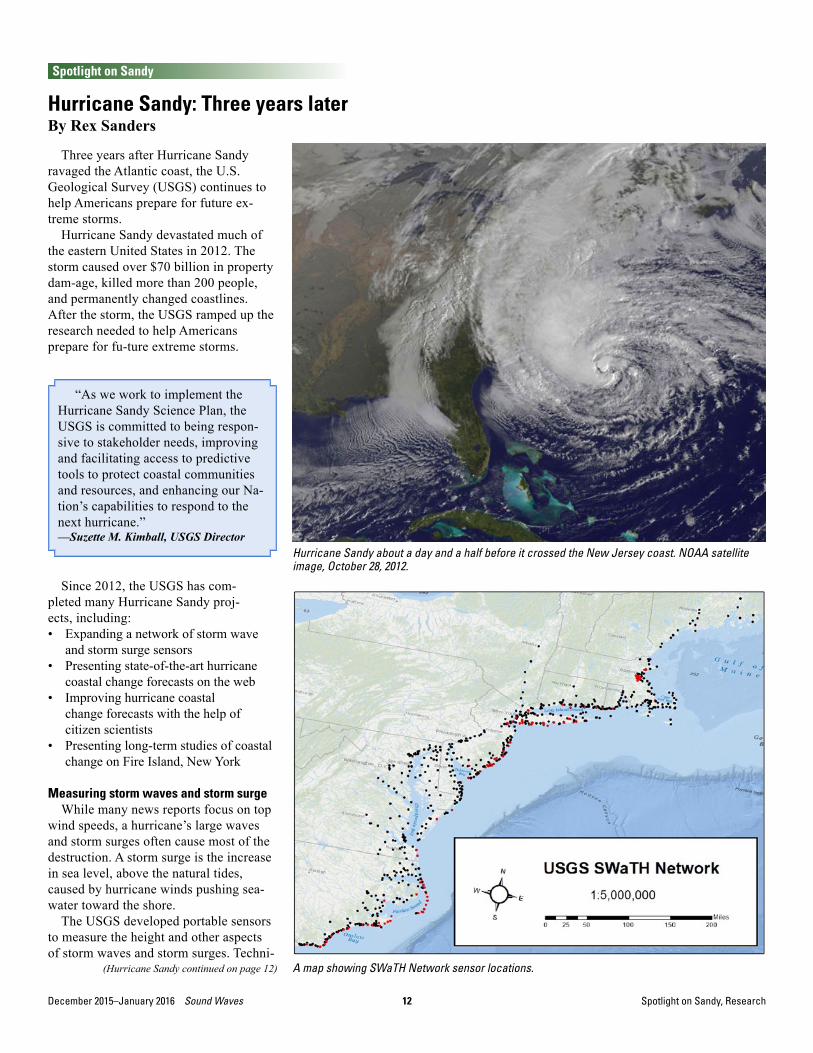
Hurricane Sandy about a day and a half before it crossed the New Jersey coast. NOAA satellite image, October 28, 2012.

A map showing SWaTH Network sensor locations.(Hurricane Sandy continued on page 12)

“As we work to implement the Hurricane Sandy Science Plan, the USGS is committed to being respon-sive to stakeholder needs, improving and facilitating access to predictive tools to protect coastal communities and resources, and enhancing our Na-tion’s capabilities to respond to the next hurricane.” —Suzette M. Kimball, USGS Director


Spotlight on Sandy, continued


cians place the sensors in the predicted path of an approaching hurricane. Some sensors transmit live data, which helps emergency responders find the worst damage. After the storm, scientists use the data to improve storm wave and storm surge forecasts; engineers use the data to design storm-resistant buildings and roads; and coastal geologists use the data to learn more about how dunes pro-tect coastlines.

However, Hurricane Sandy was so large that the USGS did not have enough sensors or a quick enough installation process to cover all of the affected areas.

Using Hurricane Sandy recovery funds, the USGS bought more sensors and established the Surge, Wave, and Tide Hydrodynamic (SWaTH) Network. The SWaTH network runs from North Caro-lina to Maine.

To speed up sensor installation, USGS staff bolted pipes to storm-resistant walls, piers and other facilities, and then recorded the precise location and eleva-tion using GPS receivers. As a hurricane approaches, technicians can quickly drop sensors into these pipes.

Scientists have found new uses for Hurricane Sandy storm surge and storm wave data from New York. A recent study (<http://soundwaves.usgs.gov/2015/09/spotlight.html>) prepared in cooperation with the Federal Emergency Management

Agency (FEMA) looked at how damage estimates change as more information becomes available. FEMA and others use damage estimates to declare disasters, prioritize relief, and guide reconstruction.

“The results from this new study dem-onstrated how the additional resolution and accuracy of flood depictions resulting from these efforts greatly improved the

damage estimates,” said Chris Schubert, a USGS hydrologist. “The storm-tide information we provided to FEMA in the immediate aftermath of Sandy is one of the building blocks for this research.”

Forecasting coastal changes caused by hurricanes

A major hurricane like Sandy ap-proaches your area, and you have ques-tions. Is my home in danger? Will my evacuation routes work? What could my favorite beach look like afterwards?

With a couple of mouse clicks or fin-ger taps, you can “see” past, present, and future hazards for most of America’s coastline. The USGS Coastal Change Hazards portal (<http://marine.usgs.gov/coastalchangehazardsportal/>) can help citizens prepare for emergencies and help resource managers plan to restore ecosys-tems. The USGS expanded and improved the portal using long-term research and Hurricane Sandy recovery funds.

The portal runs in any modern web browser on a desktop computer, tablet, or smart phone. The USGS designed it for a wide range of audiences, from govern-

Craig Brown, a USGS hydrologist, installs a sensor pipe for the SWaTH Network.

(Hurricane Sandy continued from page 12)

The USGS coastal change forecast for Fire Island, New York, released before Hurricane Sandy, with a photo showing what actually happened. The photo confirms a successful inundation forecast.

(Hurricane Sandy continued on page 14)




ment planners to people worried about a looming hurricane.

“As a storm approaches the coast we will be able to make timely forecasts of coastal change, and identify where the greatest threats are,” said Hilary Stockdon, a USGS research oceanogra-pher. “As the storm’s landfall location becomes more certain, the forecast is updated to provide more accurate in-formation on what to expect in terms of coastal change.”

A video demonstration of the por-tal (< https://www.youtube.com/watch?v=ZvlITDs9PII>) shows how someone living in Rodanthe, North Caro-

lina, can use the portal to answer the ques-tion: How much beach erosion is occur-ring in my community?

“Our nation’s coastlines are constantly changing landscapes that pose unique management challenges,” said Suzette Kimball, USGS director. “This new USGS portal is truly one-of-a-kind, pro-viding a credible foundation for making decisions to protect resources, reduce risk, and prevent economic losses.”

Citizen scientists improve hurricane coastal change forecasts

You can help the USGS improve hurri-cane coastal change forecasts. The iCoast (<http://coastal.er.usgs.gov/icoast/>) web site lets you compare photographs taken by USGS scientists from airplanes before and after major hurricanes.

In iCoast, you click a few boxes iden-tifying coastal features such as beaches and buildings, and changes such as dune erosion and dead vegetation. This helps researchers improve forecasts of coastal changes caused by hurricanes.

“Computers cannot yet automatically identify damages and geomorphic chang-es to the coast from aerial photographs,” said Sophia B. Liu, a USGS research geographer who led the development of iCoast. “Human intelligence is still need-ed to finish the job.”

Over 700 citizen scientists have scruti-nized nearly 8,000 before-and-after pho-tos from Hurricane Sandy. You can sign up at iCoast <http://coastal.er.usgs.gov/icoast/> to help the USGS inspect more than 8,000 new Hurricane Joaquin shots.


The USGS Coastal Change Hazards Portal on a tablet computer.

Video demonstrating the USGS Coastal Change Hazards Portal (< https://www.youtube.com/watch?v=ZvlITDs9PII>). The portal has changed slightly since the production of this video.

USGS geologist Karen L.M. Morgan taking aerial photographs after a hurricane.

(Story continued on page 15)




Long-term research: Fire Island, New YorkThe Fire Island Coastal Change

(<http://coastal.er.usgs.gov/fire-island/>) website presents over a decade of re-search on changes to the island’s beaches and dunes. Fortunately, many years of USGS research preceded Hurricane Sandy, so we can compare conditions on Fire Island before and after the storm.

“The website is intended to provide our Federal, State, and local partners and stakeholders with an access point to the large body of science we have


Screen shot of iCoast, where you can help improve forecasts of hurri-cane coastal change by comparing before and after photos.

Hurricane Sandy destroyed or damaged many ocean front homes on Fire Island, NY. (Photo: Cheryl Hapke, USGS)

USGS research geologist Cheryl Hapke (center) explains to National Park Service manager Mike Bilecki (right) how instruments mounted on per-sonal watercraft will measure depths in shallow water. USGS engineering technician BJ Reynolds is beside the watercraft.

Looking east toward Fire Island lighthouse. The flat, sandy overwash sheets are where Hurricane Sandy destroyed the dunes. USGS photo-graph by Cheryl Hapke.

produced,” said Cheryl Hapke, research geologist and currently Director of the USGS St. Petersburg Coastal and Marine Science Center.

Fire Island is the longest barrier island on the south shore of Long Island, New York. A barrier island is long and narrow, running parallel to the coast, separated from the mainland by shallow water. Most of the island is part of Fire Island National Seashore, managed by the Na-tional Park Service.

Scientists and land managers can use research from Fire Island on other barrier islands up and down the U.S. Atlantic coast, and along the Gulf of Mexico.

“Barrier islands are dynamic systems that also provide protection from future storms to the built environment,” Hapke said. “A thorough understanding of the long-term and short-term evolution of barrier islands can lead to models that better predict future changes to the coast-al system at Fire Island.”


Scientists from the U.S. Geological Survey (USGS) St. Petersburg Coastal and Marine Science Center participated in the Great American Teach-In on November 18, 2015. The Great American Teach-In, a na-tionwide event, has been taking place since 1994 and is an opportunity for members of the community to participate in kin-dergarten through high school classes and provide a personal perspective on their ca-reer choices and experiences pertaining to education and overcoming obstacles, both academically and professionally.

Scientists from the St. Petersburg Sci-ence Center have been participating in the Great American Teach-In since 1999 (<http://soundwaves.usgs.gov/2003/01/outreach4.html>). This year the Cen-ter had record participation—engaging a total of 1,088 kindergarten through 8th grade students at six local schools on topics including coastal erosion pro-cesses, sediments, microfossils, and ocean acidification.

Joe Long and David Thompson vis-ited Douglas L. Jamerson, Jr. Elemen-tary School and gave a coastal erosion presentation and demonstration to five kindergarten classes, as well as 1st and 2nd grade classes, speaking to about 160 students. Joe commented, “The students loved the presentation and asked great questions about waves and beaches.”

Nathaniel Plant participated in the Teach-In at Skyview Elementary School and presented coastal erosion hazards. He demonstrated barrier island response to category 1, 2, and 3 hurricanes, repre-sented by varying fan speeds. Nathaniel spoke to six 4th grade classes and 120 stu-dents. He received an excellent comment from a girl who offered an explanation of the erosion model: “I think energy from the water makes the sand move and causes the changes.”

Kara Doran gave a presentation titled “Why study sand?” at Sawgrass Lake El-ementary School. Eighty students from 4 classes ranging from grades 1–5 looked at sand samples from around the world and

talked about how hurricanes move sand around on beaches.

Kathryn Smith spoke to 6th graders at Thurgood Marshall Middle School and discussed the importance and use of mi-crofossils in coastal studies and provided 80 students the opportunity to examine diatom specimens from various environ-ments under microscopes.

Kyle Kelso presented a coring and stratigraphy demonstration at Azalea El-ementary School. He discussed lithology (the study of rocks) and provided a hands-

on opportunity for 240 children, from 12 classes ranging from 1st to 5th grades, to participate in steps involved in sediment collection and analysis.

Kira Barrera spoke at Plato Academy. She gave a presentation on ocean acidi-fication to 20 classes and approximately 400 students. Students had the opportunity to participate in several experiments dem-onstrating the effects of ocean acidifica-tion on coastal environments. One student stated, “I learned how water changes and how air affects water.”

Outreach

Outreach

USGS St. Petersburg Coastal and Marine Science Center Participates in Great American Teach-Inby Kira Barerra

Students add carbon dioxide (CO2) from their breath to a sample of seawater in order to observe the process of ocean acidification.

A coastal erosion model simulates barrier island response to storms. Left image shows the model before a simulated storm; right image shows the model after a simulated storm.

17 Sound Waves December 2015–January 2016Outreach

Outreach, continued

USGS Educates K-12 Students, Public at Fifth Annual St. Petersburg Science FestivalBy Kaitlin Kovacs

Collecting mini-sediment cores, build-ing up a coastline to endure storm surge from hurricane winds, identifying mana-tees via scar patterns, and hopping aboard wave runners—these hands-on demonstra-tions had attendees of the Fifth Annual St. Petersburg Science Festival excited about U.S. Geological Survey (USGS) science.

More than 10,000 attendees visited the festival, held October 16–17, 2015, at Poynter Park, adjacent to the University of South Florida St. Petersburg campus in St. Petersburg, Florida. The annual science event engages children, families, and the public in hands-on science, tech-nology, engineering, and math (STEM) activities. The festival also emphasizes the role of the arts in innovation, broad-ening the traditional STEM focus to STEAM (STEM plus the arts).

The USGS St. Petersburg Coastal and Marine Science Center partnered with the USGS Wetland and Aquatic Research Center for Friday’s “School Day Sneak Peek” event. Kaitlin Kovacs (Wetland and Aquatic Research Center) spearhead-ed the exhibit “Manatee Identification,” a hands-on activity that targeted two Florida science curriculum standards and introduced hundreds of fifth graders to the USGS manatee research and photo-identification program (<http://fl.biology.

usgs.gov/Manatees/manatees.html>). St. Petersburg Science Center staff members Kathryn Smith, Alisha Ellis, Kira Barrera, Kara Doran, and Sandra Coffman also partici-pated in the school day event.

For Saturday’s event, the St. Peters-burg Science Center presented three more booths: “Secrets of the Seafloor,” “Understanding the Big Picture with Little Friends,” “Coastal Hazards and Change,” and displayed two wave runners and the research vessel (R/V) Sallenger. Twenty staff members vol-unteered for Saturday’s event, including Kira Barrera, Elsie McBride, Nicole Khan, Caitlin Reynolds, Jaimie Little, Shelby Stoneburner, Chris Smith, Joseph Long, Tim Nelson, Soupy Dalyander, Kara Doran, Davina Passeri, Robert Jenkins, Nancy DeWitt, Max Tuten, Chelsea Stark, Jennifer Miselis, Steven Douglas, and Joseph Terrano. Kira Barrera organized the USGS exhibi-tors and volunteers.

The national Science Festival Alliance (<http://sciencefestivals.org>) website, which includes the St. Petersburg festival, offers more in-formation about science and technol-ogy festivals.

Visit the St. Petersburg Science Festi-val Facebook page (<https://www.face-book.com/St-Petersburg-Science-Festi-val-133812573354577/>) for video, photos, and more details about the festival.

Students at the “School Day Sneak Peek” event visited the USGS exhibit to learn how researchers use scarring patterns to identify manatees.

USGS scientists led festival attendees in hands-on activities to learn about USGS research programs, including coastal hazards and change.

Festival attendees collected mini sediment cores and peered through microscopes at diatoms as part of the USGS activities at the 2015 St. Petersburg Science Festival.

https://www.facebook.com/St-Petersburg-Science-Festival-133812573354577/










Meetings

Meetings

A-ICC Training Courses on Ocean Acidificationby Kira Barerra

U.S. Geological (USGS) oceanogra-pher Lisa Robbins serves on the Ocean Acidification International Coordination Centre (OA-ICC) Advisory Board and is chair of capacity building (<https://www.iaea.org/ocean-acidification/page.php?page=2181>). The OA-ICC works to promote, facilitate, and communi-cate global activities on ocean acidifica-tion and acts as a hub, bringing together scientists, policy makers, media, schools, the general public and other ocean acidifi-cation stakeholders.

A key component of the OA-ICC ap-proach is capacity building (<https://www.iaea.org/ocean-acidification/page.php?page=2197>) through trainings and workshops, which provide students and scientists entering the field, in particular from under-resourced countries, access to high-quality training so they can set up pertinent experiments, avoid typical pitfalls, and ensure comparability with other studies.

OA-ICC-sponsored workshops and training on ocean acidification have been held all over the world, including Brazil, Chile, China, Italy, and South Africa. The events cover impacts of ocean acidifica-tion on coastal communities, provide exposure to fundamentals, standards, and experimental design within the field, and emphasize main topics such as: coastal communities dependent on fisheries and aquaculture; coral reef and marine-based tourism under environmental change; modeling of biological, economic and sociological impacts; potential societal action and adaptation; governments and legislation. In addition, they bring together participants from a range of dif-ferent backgrounds including natural sciences, economics, sociology, industry, and government.

The last two capacity building work-shops took place October 19–24, 2015, at Xiamen University in China, and November 1–7, 2015, in Cape Town, South Africa. The training included lec-tures as well as hands-on experiments in small groups. Participants were trained on critical topics including: the carbon

dioxide (CO2) system and its measure-ment, instrumentation available for mea-suring seawater chemistry parameters, software packages used to calculate CO2 system parameters, and key aspects of ocean acidification experimental design, including manipulation of seawater chem-istry, biological perturbation approaches, and lab- and field-based methods for measuring organism calcification and other physiological responses to seawater chemistry changes, including nuclear and isotopic techniques.

In addition to helping to organize the international workshops, Robbins pre-sented information on instrumentation and available software, such as CO2calc that she and her team have developed and published (<http://soundwaves.usgs.gov/2011/03/research4.html>). Data collected from different USGS projects on ocean acidification from the poles (<http://coastal.er.usgs.gov/ocean-acidification/research/polar.html>) to the tropics (<http://coastal.er.usgs.gov/

flash/>) was used as examples and discus-sion points during the courses.

The workshops increased scientists’ capacity to measure and study ocean acidi-fication and provided a rare opportunity for collaboration and networking among scientists working on ocean acidification across the world, as well as initiated and deepened connections with the Global Ocean Acidification Observing Network (GOA-ON; <http://www.goa-on.org/>). OA-ICC sponsored E-learning mod-ules are now being developed from the workshop lectures by USGS volunteer/St. Petersburg Community College Sci-ence Teacher Sharon Gilberg and Rob-bins. These will be posted on the USGS website and, among other activities, will be used for pre-workshop preparation by participants.

The next OA-ICC sponsored workshops will occur in Mozambique, Africa (March 2016) and Mexico (Fall 2016), with ad-ditional workshops being discussed by the OA-ICC.

The first Latin- American Ocean Acidification (LAOCA) Workshop held in Dichato, Chile, sponsored by the OA-ICC and the Universidad de Concepcion, Institute de Musels, Chile.

https://www.iaea.org/ocean-acidification/page.php?page=2181






http://soundwaves.usgs.gov/2011/03/research4.html

http://soundwaves.usgs.gov/2011/03/research4.html

http://coastal.er.usgs.gov/ocean-acidification/research/polar.html

http://coastal.er.usgs.gov/ocean-acidification/research/polar.html

http://coastal.er.usgs.gov/flash/

http://coastal.er.usgs.gov/flash/


Publications

Publications

Bernier, J.C., Douglas, S.H., Terrano, J.F., Barras, J.A., Plant, N.G., and Smith, C.G., 2015, Land-cover types, shoreline positions, and sand extents derived From Landsat satellite imagery, Assateague Island to Metompkin Island, Maryland and Virginia, 1984 to 2014: Data Series 968 [http://dx.doi.org/10.3133/ds968].

Cochrane, G.R., Dartnell, P., Johnson, S.Y., Greene, H.G., Erdey, M.D., Dieter, B.E., Golden, N.E., Endris, C.A., Hartwell, S.R., Kvitek, R.G., Davenport, C.W., Watt, J.T., Krigsman, L.M., Ritchie, A.C., and others, 2015, California State Waters map series—Offshore of Scott Creek, California: Open-File Report 2015–1191 [http://dx.doi.org/10.3133/ofr20151191].

Doran, K.S., Howd, P.A., and Sallenger, J., Asbury H., 2015, Detecting sea-level hazards: Simple regression-based methods for calculating the acceleration of sea level: Open-File Report 2015–1187, 34 p. [http://dx.doi.org/10.3133/ofr20151187].

Enwright, N.M., Griffith, K.T., and Osland, M.J., 2015, Incorporating future change into current conservation planning: Evaluating tidal saline wetland migration along the U.S. Gulf of Mexico coast under alternative sea-level rise and urbanization scenarios: Data Series 969 [http://dx.doi.org/10.3133/ds969].

Erikson, L.H., Hegermiller, C.A., Barnard, P.L., Ruggiero, P., and van Ormondt, M., 2015, Projected wave conditions in the Eastern North Pacific under the influence of two CMIP5 climate scenarios: Waves and coastal, regional and global processes, v. 96, Part 1, p. 171–185. [http://dx.doi.org/10.1016/j.ocemod.2015.07.004]

Geist, E.L., 2015, Non-linear resonant coupling of tsunami edge waves using stochastic earthquake source models: Geophysical Journal International, v. 204, no. 2, p. 878–891. [http://dx.doi.org/10.1093/gji/ggv489]

Giese, G.S., Williams, S.J., and Adams, M., 2015, Coastal landforms and processes at the Cape Cod National Seashore, Massachusetts—A primer: Circular 1417, 94 p. [http://dx.doi.org/10.3133/cir1417].

Gutierrez, B., Plant, N.G., Thieler, E.R., and Turecek, A., 2015, Using a Bayesian network to predict barrier island geomorphologic characteristics: Journal of Geophysical Research. [http://dx.doi.org/10.1002/2015JF003671]

Guy, K.K., 2015, Back-island and open-ocean shorelines, and sand areas of the undeveloped areas of New Jersey barrier islands, March 9, 1991, to July 30, 2013: Data Series 960 [http://dx.doi.org/10.3133/ds960].

Johnson, C., Swarzenski, P.W., Richardson, C.M., Smith, C.G., Kroeger, K.D., and Ganguli, P.M., 2015, Ground-truthing electrical resistivity methods in support of submarine groundwater discharge studies: Examples from Hawaii, Washington, and California: Journal of Environmental and Engineering Geophysics, v. 20, no. 1, p. 81–87. [http://dx.doi.org/10.2113/JEEG20.1.81]

Kuffner, I.B., Yates, K.K., Zawada, D.G., Richey, J.N., Kellogg, C.A., and Toth, L.T., 2015, USGS research on Atlantic coral reef ecosystems: Fact Sheet 2015–3073, 2 p. [http://dx.doi.org/10.3133/fs20153073].

Osland, M.J., Enwright, N.M., Day, R.H., Gabler, C.A., Stagg, C.L., and Grace, J.B., 2016, Beyond just sea-level rise: Considering macroclimatic drivers within coastal wetland vulnerability assessments to climate change: Global Change Biology, v. 22, no. 1, p. 1–11 [http://dx.doi.org/10.1111/gcb.13084].

Palmsten, M.L., Splinter, K.D., Plant, N.G., and Stockdon, H.F., 2014, Probabilistic estimation of dun retreate on the Gold Coast, Australia: Shore and Beach, v. 82, no. 4, p. 35–43 [https://pubs.er.usgs.gov/publication/70159345].

Prouty, N.G., Swarzenski, P., Mienis, F., Duineveld, G., Demopoulos, A., Ross, S.W., and Brooke, S., 2016, Impact of Deepwater Horizon Spill on food supply to deep-sea benthos communities: Estuarine, Coastal and Shelf Science, v. 169, p. 248–264 [http://dx.doi.org/10.1016/j.ecss.2015.11.008].

Rode, K.D., Wilson, R.R., Regehr, E.V., St. Martin, M., Douglas, D., and Olson, J., 2015, Increased land use by Chukchi Sea polar bears in relation to changing sea ice conditions: PLoS ONE, v. 10, no. 11 [http://dx.doi.org/10.1371/journal.pone.0142213].

Rosencranz, J.A., Ganju, N.K., Ambrose, R.F., Brosnahan, S.M., Dickhudt, P.J., Guntenspergen, G.R., MacDonald, G.M., Takekawa, J.Y., and Thorne, K.M., 2015, Balanced Sediment Fluxes in Southern California’s Mediterranean-Climate Zone Salt Marshes: Estuaries and Coasts, p. 1–15 [http://dx.doi.org/10.1007/s12237-015-0056-y].

Schwab, W.C., Baldwin, W.E., and Denny, J.F., 2016, Assessing the impact of Hurricanes Irene and Sandy on the morphology and modern sediment thickness on the inner continental shelf offshore of Fire Island, New York: Open-File Report 2015–1238, 26 p. [http://dx.doi.org/10.3133/ofr20151238].

Smith, J.E., Bentley, S.J., Snedden, G.A., and White, C., 2015, What Role do Hurricanes Play in Sediment Delivery to Subsiding River Deltas? Scientific Reports, v. 5, p. 17582 [http://dx.doi.org/10.1038/srep17582].

Stockdon, H.F., Thompson, D.M., Plant, N.G., and Long, J.W., 2014, Evaluation of wave runup predictions from numerical and parametric models: Coastal Engineering, v. 92, p. 1–11 [http://dx.doi.org/10.1016/j.coastaleng.2014.06.004].

Stoker, J.M., Brock, J.C., Soulard, C.E., Ries, K.G., Sugarbaker, L.J., Newton, W.E., Haggerty, P.K., Lee, K.E., and Young, J.A., 2016, USGS lidar science strategy—Mapping the technology to the science: Open-File Report 2015–1209, 39 p. [http://dx.doi.org/10.3133/ofr20151209].

Tess E. Busch, Flannery, J.A., Richey, J.N., and Stathakopoulos, A., 2015, The relationship between the ratio of strontium to calcium and sea-surface temperature in a modern Porites astreoides coral: Implications for using P. astreoides as a paleoclimate archive: Open-File Report 2015–1182, 15 p. [http://dx.doi.org/10.3133/ofr20151182].

Recent Publications


Publications, continued

Publicatons

Thorne, K.M., Buffington, K.J., Elliott-Fisk, D.L., and Takekawa, J.Y., 2015a, Tidal Marsh Susceptibility to Sea-Level Rise: Importance of Local-Scale Models: Journal of Fish and Wildlife Management, v. 6, no. 2, p. 290–304 [http://dx.doi.org/10.3996/062014-JFWM-048].

Thorne, K.M., Dugger, B.D., Buffington, K.J., Freeman, C.M., Janousek, C.N., Powelson, K.W., Gutenspergen, G.R., and Takekawa, J.Y., 2015b, Marshes to mudflats—Effects of sea-level rise on tidal marshes along a latitudinal gradient in the Pacific Northwest: Open-File Report 2015–1204 [http://dx.doi.org/10.3133/ofr20151204].

Tinker, M.T., Hatfield, B.B., Harris, M.D., and Ames, J.A., 2016, Dramatic increase in sea otter mortality from white sharks in California: Marine Mammal Science, v. 32, no. 1, p. 309–326 [http://dx.doi.org/10.1111/mms.12261].

Toth, L.T., Aronson, R.B., Cheng, H., and Edwards, R.L., 2015a, Holocene

variability in the intensity of wind-gap upwelling in the tropical eastern Pacific: Paleoceanography, v. 30, no. 8, p. 1113–1131 [http://dx.doi.org/10.1002/2015PA002794].

Toth, L., Kuffner, I.B., Cheng, H., and Edwards, R.L., 2015b, A new record of the late Pleistocene coral Pocillopora palmata from the Dry Tortugas, Florida reef tract, USA: Palaios, v. 30, no. 12, p. 827–835 [http://dx.doi.org/10.2110/palo.2015.030].

Valentine, P.C., and Gallea, L.B., 2015, Seabed maps showing topography, ruggedness, backscatter intensity, sediment mobility, and the distribution of geologic substrates in Quadrangle 6 of the Stellwagen Bank National Marine Sanctuary Region offshore of Boston, Massachusetts: Scientific Investigations Map 3341, 34 p. [http://dx.doi.org/10.3133/sim3341].

Walton, M.A.L., Gulick, S.P.S., Haeussler, P.J., Roland, E.C., and Trehu, A.M.,

2015, Basement and regional structure along strike of the Queen Charlotte Fault in the context of modern and historical earthquake ruptures: Bulletin of the Seismological Society of America, v. 105, no. 28, p. 1090–1105 [http://dx.doi.org/10.1785/0120140174].

Witter, R.C., Carver, G.A., Briggs, R., Gelfenbaum, G.R., Koehler, R.D., La selle Seanpaul M., Bender, A.M., Engelhart, S.E., Hemphill-Haley, E., and Hill, T.D., 2015, Unusually large tsunamis frequent a currently creeping part of the Aleutian megathrust: Geophysical Research Letters [http://dx.doi.org/10.1002/2015GL066083].

Woodroffe, C., Rogers, K., Mckee, K.L., Lovelock, C., Mendelssohn, I., and Saintilan, N., 2016, Mangrove sedimentation and response to relative sea-level rise: Annual Review of Marine Science, v. 8, p. 243–266 [http://dx.doi.org/10.1146/annurev-marine-122414-034025].

fieldwork investigating the offshore queen charlotte ... · system in southeastern alaska, and its...

Documents