Field Evaluation of a Low-Cost Strapdown IMU by means GPS

RAUL DOROBANTU*)

AND BENEDIKT ZEBHAUSER*)

Abstract

The paper presents a field experiment for a low-cost strapdown-IMU/GPS combination, with datapostprocessing for the determination of 2-D components of position (trajectory), velocity andheading. In the present approach we have neglected earth rotation and gravity variations, because ofthe poor gyroscope sensitivities of our low-cost ISA (Inertial Sensor Assembly) and because of therelatively small area of the trajectory. The scope of this experiment was to test the feasibility of anintegrated GPS/IMU system of this type and to develop a field evaluation procedure for such acombination. Also a hardware synchronisation between GPS time and the IMU’s data acquisitiontime scale is presented.The authors briefly describe the IMU strapdown mechanisation procedure, the DGPS dataprocessings and the implementation of a suboptimal Linear Kalman Filter (LKF), with the systemlinearization exemplified for the 2-D case.Plots of test results, concerning the KF update for the carrier phase or pseudorange DGPS solutions,made at regular epochs of integer seconds, as well as comparisons between the INS and the GPStrajectory solutions are given. The results demonstrate the feasibility of our cost-effective IMU/GPSintegration, with accuracy improvements from ca. 20 m (IMU alone) toward the meter domain (forthe combination) depending on good GPS reception conditions. The precise carrier-phase DGPSsolution, with an accuracy in the cm domain, was used as reference for the strapdown-mechanized-IMU’s performance evaluation.

I. Introduction

Since 1978 one has recognised the advantages of tightly-coupled GPS/INS (Global PositioningSystem /Inertial Navigation System) systems [1]. The idea is to combine the advantage of the short-

term precision of INS and the long-termstability of GPS. With the significantdecrease of inertial sensor prices [2, 3](micromachined accelerometers and rategyroscopes), the rapid increase ofcomputing power (permitting the on-lineapproach applied to strapdownnavigation systems) and with thetendency of using standard software forsuch GPS/INS systems [1], one can lookforward for a much wider use of aidedGPS inertial navigation. The goal of thispaper is to present the results from afield test with a combination of a low-cost strapdown ISA (Inertial SensorAssembly) unit [4] with GPS aiding. Acentral item has been the test of thefeasibility of a processing algorithm

*) Technische Universität München, Institut für Astronomische und Physikalische Geodäsie Arcisstr. 21, D-80290 München, Germany; email: raul@alpha.fesg.tu-muenchen.de

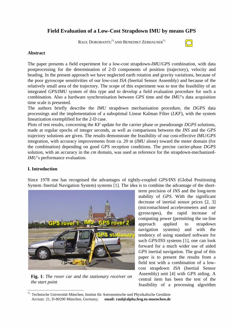
Fig. 1: The rover car and the stationary receiver onthe start point

using a simplified linear Kalman filter [5, 6] with only 5 state-variables. A 2-D solution of this typebenefits from the precision information of position, velocity and heading, derived from a referencecarrier-phase DGPS (Differential GPS) solution; a variety of simulations runs has been carried outwith two specific GPS solutions (Pseudorange and carrier phase DGPS).The study has also permitted to elaborate a field test methodology for IMU (Inertial MeasurementUnit) units. The tests have carried out with a car carrying on its roof a platform equipped with twoGPS-antennas and one IMU unit. There are neglected the g - variations and the Earth rotation rate,because of the small dimensions of the test area (some 100×100 m), of the relative low carvelocities (about 5 m/s, that is about 18 km/h) and of the reduced rate sensitivity of the usedgyroscopes.The mutual benefit of an INS/GPS combination should be the compensation of the IMU(INS) driftand the coverage of long period unavailability of the GPS [7] (in city environments, in tunnels, etc.)or of imprecision caused by interference by multipath reflections. By using an appropriatesuboptimal Kalman filter (KF), one can take advantage of a good dynamic description of the IMU,combined with the unbiased observations of the available GPS data.In the paper the INS/GPS measuring system is described. We also give an IMU strapdowncompensation algorithm (implemented also in an interactive version under Simulink - Matlab) andthe postprocessing solution for a reference navigation path, together with some alternative KFsimulations (observations provided every second and every 4 s respectively or with random GPSupdating).

II. Experiment description

In Fig. 1 the rover car is shown equipped with two GPS receiver antennas mounted on the car roofon a wooden plate at a fixed distance of 1.40 m. One can see the ISA unit, rigidly fixed in the middleof the platform. A stationary GPS receiver is used to generate the DGPS (Differential GPS)solutions.The GPS system permits the accurate computation of the position (carrier-phase DGPS) and thevelocity of the ISA’s centre of mass. One can also derive a heading reference from the GPS solutionand deliver it as update for the angular azimuth in the KF (normally furnished from the z-axis rategyroscope).

Fig. 2 View of the opened ISAunit: the three-axialaccelerometer and a one-axisgyroscope

This first test has been carried out on „Theresienwiese“ in Munich.The ISA unit, of type iMAR [4], uses a triaxial accelerometer realised by quartz micromachinedtechnology [8] and a triad of quartz vibrating rate gyroscopes [9], based on the Coriolis-forceprinciple.The inertial sensors are mounted in an aluminium cube by iMAR

with an unique referencemounting surface. Fig. 2 shows the opened cube, here mounted on a rotating platform for calibrationin our laboratory.The analog signal furnished by the ISA unit is acquired via an A/D multiplexed conversion unit(Type DAQPad - MIO - 16XE - 50 from NATIONAL INSTRUMENTS

[10]), with a 16 bit/channelresolution. A sampling rate of 25 Hz was chosen; data are stored on a TOSHIBA

PC - Notebook inbinary or ASCII format files, with 8 columns: 3 channels of accelerometer data, 3 channels ofgyroscope data (the rotating rate information), one channel of the inertial-cube interior temperatureinformation and one channel with time-reference information (in analog form), necessary to assurethe synchronisation between the INS and the GPS systems.In this starting phase of the experiment the synchronisation is carried out by simultaneouscontinuous registration, on the 8-th channel (#7) of the data converter, of a time signal with 0.1 sduration. It is derived from the standard PPS (one Pulse Per Second) output signal of a GPS receiver(here, for comparison, derived from an ASHTECH

receiver, respectively from the rover TRIMBLE

receiver). To realise also an absolute reference time scale, a supplementary 0.5 s asynchronoussignal is generated manually, at an arbitrarily observed GMT time, displayed on the GPS receiverpanel, and electronically superimposed to the same # 7 channel of the time reference (see Fig. 3).The realised electronic (the monostable multivibrators, the logic OR and the attached LED displays -for the PPS signal, respectively for the asynchronous one) is mounted in a small separate case (seeFig. 4) and connected by coaxial cables to the PPS output signal (GPS receiver) and the input of the8-th channel of the A/D converter.Because of the great duration difference (5:1) between the two time signals one can automaticallydetect any asynchronous event without difficulty. This enables an absolute marking of the inertialdata registration on the associated time scale.

Fig. 3 Time scale generated onthe 8-th channel of the inertialdata file (PPS synchronous andasynchronous event signals)

Nevertheless one must take into account the absolute time difference between the recorded UTCasynchronous event and the GPS-time reference SoW (Second of GPS Week) for the satellitepositioning solution. At the time of the experiment this difference was [11]:

GPS-time - GMT-time = +12 s (i.e., at 14.05.1998 the GPS time was 12 s ahead of UTC ) .

In this 2-D experiment no initial alignment was carried out. The alignment is deduced in the courseof the experiment from the GPSpositioning data. Of course, one must takeinto account a short initialisation phase ofabout 10 to 15 min at the beginning of theGPS session.

Fig. 4 View of the hardware for theanalog time signals (in the laboratoryexperimentation phase, connected to aTrimble GPS receiver)

III. IMU’s strapdown mechanisation

Using the calibration data for the inertial sensor assembly (bias, linear scale factors, gyroscopestriad non-orthogonality) delivered from the manufacturer and the supplementary calibrationmeasurements made in our laboratory the error model of the inertial sensors is validated. The mostimportant measurements carried out in our laboratory are: the evaluation of the noise behaviour ofthe inertial data sets, static accelerometer calibrations - to determine the supplementary non-linearterms of the static transfer characteristics, considered only to degree 2 -, as well as the establishmentof the non-linear time and temperature behaviour of the accelerometer’s drift and scale factors andthe non-orthogonality of the accelerometer’s triad. The complex dependencies between the electricaloutput signal u [V] of an inertial sensor (here an accelerometer) and the specific forces f, theelapsed time t and the temperature T take the following analytical form:

u D H k k t k t k f k f k f k f k f= + + + ⋅ + ⋅ + ⋅ + ⋅ + ⋅ + ⋅ + ⋅ +0 01 022

1 1 2 12

3 13

12 2 13 3no no

+ ⋅ ⋅ + ⋅ ⋅ + ⋅ + ⋅12 1 2 13 1 3 41 422cc cck f f k f f k T k T , (1)

where we used the following notation:

D = dead zone (under this threshold one has no signal),H = hysteresis,

0k = bias (a new value for each new use of the instrument),

01 02k k, = drift coefficients (modelling the linear and the quadratic variations with time t,respectively),

1 2 3k k k, , = coefficients of the polynomial approximation of the non-linear responsecharacteristic to the specific force along the sensible input axis,

1 2 3f f f, , = specific forces, along the three input axes (denoted 1, 2 and 3),

12 13no no,k k = coupling coefficients between the input axes, due to non-orthogonality,

12 13cc cc,k k = cross - coupling coefficients,

41 42k k, = coefficients of the polynomial dependence (linear and quadratic) of the sensoroutput signal from temperature T

The inertial data are processed in a strapdown mechanisation [12], based on the followingexpression for a one-component specific force in a body reference system (see Fig. 5, that explainsthe forces

considered, acting upon the seismic massof the accelerometer), as a function of thelinear acceleration x

ba , the apparent

centripetal acceleration cf xba _ and the

corresponding axial component of the

static gravitational acceleration xbg (the

superscripts b denote the vectorcomponents in the body reference system):

m x xb

cf xb

xbf a a g_ _= + − . (2)

The corresponding vectorial form (withthe specific force vector now denoted by aand the correction terms of centripetal andgravity acceleration expressed in the bodycoordinate system) is:

b bnb na a v C g= − × + ⋅ωω . (3)

with:=ωω the angular velocity vector,=vb the velocity vector, given in the

coordinate system b,=Cb

n the rotation matrix from the local coordinate system n to the body coordinate system b.

Fig. 6 Flow-chart of the strapdown mechanisation

bxby

bz

ba

xba

ngcf xb

_a

Γ( )t

bvybv

zbωωx

bg

m

+ m xf

_

Fig. 5 Specific force as a function of the accelerationcomponents along a reference system firmly attachedto the moving body (example for x - axis)

U acc x_ _

GYROSCOPE 'S

SIGNAL

CORRECTION

ACCELEROMETER'S

SIGNAL

CORRECTION

2

1

3

ZUPT

−−−−−

scale factor

bias

drift

temperature

nonorthogonality

ZUPT

−−−−−

scale factor

bias

drift

temperature

nonorthogonality

U acc y_ _

U acc z_ _

xA

yA

zA

zG

yG

xGU omega x_ _

U omega z_ _

U omega y_ _

ATTITUDE

INTEGRATION

[ ]&

&

&

( , , )_

_

_

φθψ

φ θ ψωωω

= ⋅

1fx b

y b

z b

Euler

Anglesx b

y b

z b

_

_

_

ωωω

φθψ

x

y

z

a

a

a

CENTRIFUGAL

FORCE

CORRECTION

−

×

x b

y b

z b

x b

y b

z b

_

_

_

_

_

_

v

v

v

ωωω

GRAVITY

CORRECTION

+ ⋅−

⋅⋅

g

s

c s

c c

θθ φθ φ

x b

y b

z b

a

a

a

_

_

_

bt

da0∫ ( )τ τ

bt

+ =v0

4 5

[ ]bnC f= 2 ( , , )φ θ ψ

ROTATION

MATRIX

ACCEL.

INTEGR.

6

bnC

RATE

INTEGR.

7

8

nt

dv0∫ ( )τ τ

+=

nt

s0

Init. Cond.

Init. Cond.

x b

y b

z b

_

_

_

v

v

v

x n

y n

z n

_

_

_

v

v

v

x n

y n

z n

s

s

s

_

_

_

Rota

tion

−

Trajectory

( )bn TC

g

In this approach we only take into account the apparent centrifugal forces and the tilt-induced staticaccelerations (components of g assum ed to be constant). Neglected is the small Coriolis forceacting on the moving mass as a consequence of the rotation of the inertial sensors case.

Fig. 7 Strapdownmechanisation solutionof the IMU

a

b

c

d

e

f

g

h

i

j

k

a - x-axis bodyaccelerationb - x-axis body velocityc - x-axis velocity in thepseudo-inertialreference systemd - x-axis position in thepseudo-inertialreference systeme - y-axis bodyaccelerationf - y-axis body velocity

g - y-axis velocity in the pseudo-inertial reference systemh - y-axis position in the pseudo-inertial reference systemi - rotation rate about the z-axisj - rotation angle ψ about the z-axisk - x/y trajectory (only from inertial data)

As mentioned above we neglect the g - variations because of the relative small experimental areaand also the Coriolis force component resulting from the earth rotation (both of them because oflack of sensitivity of the low-cost inertial sensor system).The flow-chart of the algorithm is given in the Fig. 6. The program has been written in the Simulink- Matlab language, which enables a transparent and interactive design of the whole diversity ofsignals, also permitting an easy and rapid proof of the error model parameters.In the Fig. 7 the inertial solution of the x/y trajectory, as well as the rotation angle ψ (about the z-axis) are presented.

IV. GPS solution

The GPS solution was accurately determined by carrier phase DGPS data evaluation using OTF-(On-The-Fly) techniques, processed with the commercial SPECTRA PRECISION GEOGENIUS

software. Two separate solutions were computed, one for each pair of reference/rover receivers.Each point of the resulting trajectory of the ISA’s centre of mass (plotted as reference in the Fig. 14)represents a position solution, spaced regularly at 1 s intervals. Considered was the center pointbetween the two GPS antennas, matched with the centre of the inertial cube. The trajectory and therotation angle are determined consequently (as the arithmetic mean of successive positions of thetwo rover antennas and as the rotation angle of the spatial vector defined by the two phase centres ofthe mobile receiver antennas respectively).

Some remarks concerning the GPS solutions performed:

Because a standalone GPS receiver position solution only yields an accuracy/repeatability of sometens of meters it is common to perform measurements with 2 receivers (or more) simultaneously.

Fig. 8 DGPS constellation with 2 rover antennas on top of thecar, showing the observables as well as the estimated differencevectors between reference and rovers

Thereby one receiver is held stationary at a reference position Anearby the planned trajectory of the second (moving) receiver B,the so called rover. This is called DGPS. See Fig. 8 for theconstellation in this experiment with

[ ] [ ] Tantenna

Tantenna ZYXxZYXx 2211 ,,,,, ∆∆∆=∆∆∆=

rr .

By processing the simultaneous pseudorange measurements PR from the two receivers by thedouble differencing technique, we can eliminate systematic time dependent errors like satellite andreceiver clock biases. We can reduce other effects too and avoid, in addition, problems with highcorrelations in the parameter estimation process.The double difference observable for pseudorange DGPS can be written:

( ) ( ) ε+−−−=−−−=∇∆ jA

jB

kA

kB

jA

jB

kA

kB

jkAB SSSSPRPRPRPR (4)

with: PR = pseudorange,S = geometric distance between receiver A,B and satellite j,k ,ε = unmodeled errors (multipath, atmospheric effects) and noise.

The result of a least squares adjustment using these double difference observations providesposition differences or strictly speaking vector components ∆X, ∆Y, ∆Z in a geocentric Cartesiancoordinate system describing the vector between the reference and the rover receiver or ratherbetween their antennas. This technique using pseudoranges yields an accuracy/repeatability of about1 meter for epochwise solutions in kinematic applications. Smoothing of the pseudoranges PR bymeans of carrier phases can bring down this value to some decimeters.For even higher accuracy of a few centimeters one has to compute the position differences usingcarrier phase observations Φ: In contrast to pseudoranges PR, that are equivalent to distancemeasurements between satellite and receiver, carrier phase measurements require the determinationof cycle ambiguities N, because at the measurement epoch only the received carrier phase (fractionalpart of a cycle with λ ≅ 20 cm) and the change in the integer part (full cycles) are registered(combined in Φ), while the full range remains unknown.The double difference observable for carrier phase DGPS can be written:

( ) ( )( ) ε+−−−−=Φ−Φ−Φ−Φ=∇∆ jkAB

jA

jB

kA

kB

jA

jB

kA

kB

jkAB NSSSS

c

f

0

(5)

with: ( )jA

jB

kA

kB

jkAB NNNNN −−−= double difference ambiguity,

Φ = carrier phase observable,S = geometric distance between receiver A,B and satellite j,k ,f = carrier frequency,c0 = speed of light in vacuum,ε = unmodeled errors (multipath, atmospheric effects) and noise.

For further information on GPS techniques see also [13, 14, 15].Regarding the kinematic application we are again forced to get epochwise position solutions. Thusin contrast to stationary case we cannot accumulate observations to get higher redundancy for theestimation process which would allow us to determine these ambiguity parameters more easily.Instead we have to resolve them "on-the-way" (on-the-fly). For high precision positions we have tofix the ambiguity parameters (they are integers) in the position estimation process to their truevalues. Because the true integer values cannot reliably be found by rounding the actual float valuesfrom the least squares adjustment, they must be searched by statistical tests like χ2-tests on theresiduals of a position solution after introducing a set of possible double difference integerambiguities, or like FISHER-tests on the ratio between the best and the second best - from thestatistical point of view - position solution from different possible integer ambiguity sets. In thesoftware we used (SPECTRA PRECISION GEOGENIUS

) the search is performed with a polynomialapproach (linear regression) of the residuals in order to increase the computational speed. Thesearch hyperspace of all possible ambiguity sets is defined by a 30σ interval for every doubledifference ambiguity around its float solution. When the "true" set of all (nsat-1) double differenceinteger ambiguities is found, they are held fixed and the positions per epoch can be solved exactly .For further information on DGPS and ambiguity resolution techniques see also [16, 17].For comparison purposes the geocentric Cartesian coordinates are transformed into a localprojection to yield north, east and up components ∆N, ∆E, ∆U (≡-∆D) instead of ∆X, ∆Y, ∆Z.

Fig. 9 GPS solution of theconstant distance (1.40 m)between the two roverantennas (the greatest errorsare produced during the testrides)

For a better insight into theaccuracy of the OTF-GPSsolutions we have plotted thetime evolution of the constantbaseline between the tworover antenna centres, inreality always 1.40 m,

determined from two independent GPS solutions. From Fig. 9 one can see maximal errors about +/-5 mm, also during the intervals of car movement. It should be noted that systematic errors affectingboth antennas in the same way, that may reach up to 1 cm, are neglected in such an analysis.

The precise carrier phase DGPS solution, as well as the pseudorange DGPS solution with aprecision in the meter domain, can also be used as a bias free observation in the Kalman filter.One can derive from the GPS solution the approximate x-axis velocities, expressed in [m/s] as:

txtxtv x kk∆−=

−/)(

1, (6)

by considering the equal time-interval t∆ of the GPS solutions and determined each second(similarly for the y component), or, more elegantly, by computing the time derivatives of thesmoothly interpolated trajectory.

upper brackets: moving phases

lower brackets: non-moving phases

Fig. 10 Comparison between theGPS and INS solutions (both ofthem given in a pseudo-inertialreference system)

a

b

c

d

e

f

g

h

a - x-axis space: GPS solutionb - x-axis space: INS solutionc - rotation angle ψ : GPSsolutiond - rotation angle ψ : INS solutione - y-axis space: GPS solutionf - y-axis space: INS solutiong - x/y trajectory: GPS solutionh – independent INS and GPS

trajectories

From the comparison between theGPS and INS solutions, presentedin Fig. 10, one can see the goodmatch of the x/y trajectories andthe azimuth solutions (a detailedcomparison evidenced differencesof under one degree, after anappropriate correct alignment).

One can see also the permanently decreasing match of the IMU - determined trajectory, because ofthe continuously increasing unmodeled drift error components with time.

V. Integrated INS/GPS solution of the trajectory

To check the feasibility and the usefulness of the integration of our low-cost IMU with GPS, webuilt several different Kalman filter configurations, all working in the 2-D (two-dimensional)domain, taking into account the accurate carrier phase DGPS solution with an update every second -as well as with some slower or a random epoch updating (every 4 s or randomly ( s4=σ )). Afurther test was the use of the pseudorange DGPS solution. The INS(IMU) strapdown trajectorysolution, with short term precision, but long term drifts, is corrected either on-line or post-missionby means of the bias-free observations furnished by the GPS aiding. We made also tests for aidingevery second.We used a LKF (Linear Kalman Filter), with the IMU trajectory as reference. Because of the shortduration of our experiment, there are no noticeable temperature variations in the inertial sensor unit;so we applied in this test only a coarse bias correction at the beginning, neglecting scale-factorvariations; the compensated inertial sensor drifts are modelled only as linear time variations. Ofcourse, the complete algorithm must consider both the non-linear shape of the transfercharacteristics of gyroscopes and accelerometers, as well as the polynomial time and temperaturedependencies of the drifts. It models the slow variable drifts as Gauss-Markov processes.

The local reference system NED (North, East, Down) (denoted here with n), in which the referencetrajectory of the LKF is established (as solution of the IMU with the strapdown mechanisation), canbe assumed for this test to be an inertial frame. The linearized solution is obtained by Taylorexpansion of the real non-linear trajectory model about the reference trajectory, retaining only thefirst order term [5, 6].From the non-linear plant and observation models, in the continuous-time domain:

& ( , , ) ~( )x f x u G u= + ⋅d t t

z h x= +( , ) ~( )t tνν , (7)

where ~( )u t , ~( )νν t are the Gaussian white noise processes of the dynamic system, respectively ofthe observation, we deduce [6]:

- the discrete time non-linear model:k k kx f x w= +− −( ) ~

1 1

k k kz h x= +( ) $νν (8)

(with k kN~ ~ ( , )w Q0 , k kN~ ~ ( , )νν 0 R ),- the reference trajectory model (without noise):

k k d∗

−∗=x f x u( , )1 , (9)

- the linearized perturbed trajectory model:

δ∂

∂δk

dk k

k

k

xf x u

x x xx w= ⋅ +

=−

−∗

( , , ) ~

1

1 (10)

(with the definition of the perturbation from the nominal: δ k k kx x x= − ∗∆),

and the linearized observation model:

δ∂

∂δk k

k

k

zh x

x x xx= ⋅ +

=−

−∗

( , )

1

1 k~νν . (11)

For the derivation of the explicit forms of the above defined Jacobian matrices (the discrete

linearized state transition matrix: k

k

k

−=

=−

∗1

1

Φ∂

∂f x

x x x

( , ) and the linear observation matrix

k

k

k

Hh x

x x x=

=∗

∂∂( , )

), we are first considering the general three-dimensional form of a continuous

state equation system for a strapdown mechanisation of a body (materialised as a triad, also with alllever-arm effects omitted), moving in the reference system n assumed to be inertial:

n

n

n

n

n

n

bn b

b

t

&

&

&

( )

( )

~( )

s

v

0 I 0

0 0 0

0 0 0

s

v

I 0 0

0 C 0

0 0 E

0

a G u

ΨΨ ΨΨ

ΨΨΨΨ

=

⋅

+

⋅

+ ⋅ωω

(12)

where we denote:n

x n y n z nTs s ss = [ ]_ _ _ , the position vector in the coordinate system n

nx n y n z n

Tv = [v v v ]_ _ _ , the velocity vector, given in the coordinate system n

ΨΨ = [ ]φ θ ψ T , the Euler angles vector

bnC = the rotation matrix from the body coordinate system b to the local coordinate

system nE = the Euler angles differential equations matrix

bx b y b z b

Ta a aa = [ ]_ _ _ , the acceleration vector, measured with respect to the body

coordinate system b

bωω = [ ]_ _ _x b y b z bTω ω ω , the angular velocity vector (of the body axes) with respect

to the inertial coordinate system.The partial derivatives in eq. (10), the Jacobian matrix of the continuous, non-linear system ofequations takes the form:

Ff x u

xx x

=∗

=−

∗

∂∂

( , )d

k 1

= ⋅⋅

= •

0 I 0

0 0 C a

0 0 Ebn b

b

( )

( )

'

'

ΨΨ

ΨΨ ΨΨ ΨΨωω

, (13)

with the explicit terms for our 2-D case (with the chosen set of state variablesx = [ , , v , v , ]x

nyn

xn

yn Ts s ψ ):

0,02 ==−=

θφCCn

bD

n

b=

−

cos sin

sin cos

ψ ψψ ψ

, (14)

==θ=φ− )0,0(2 D

E [1]. (15)

The 2-D form of the continuous, linearized system matrix (evaluated at the discrete time momentst t k= , the beginning of the sampling intervals) becomes:

∂∂

ψ ψψ ψ

fx

x x

x x

=

=

+

+

= − ⋅ − ⋅⋅ − ⋅

k

k

s a c a

c a s a

xb

yb

xb

yb$

$

0 0 1 0 0

0 0 0 1 0

0 0 0 0

0 0 0 0

0 0 0 0 0

(16)

We obtain the approximate transition matrix kΦΦ = ⋅F ∆te [5], by assuming piecewise constancy of thedeterministic inertial sensor signals during the sampling interval and by retaining only the linearterm of the Taylor series:

kΦΦ ≅ I F+ ⋅ ∆ t (17)where ∆ t represents the small sampling rate interval.

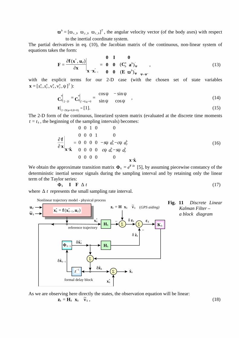
Fig. 11 Discrete LinearKalman Filter –a block diagram

As we are observing here directly the states, the observation equation will be linear:k k k kz H x= ⋅ + ~νν , (18)

+

−

+

+−

+

+

+

k k d∗

−∗=x f x u( , )1

Nonlinear trajectory model - physical process

du

k~w

ΣΣ kK

k −1ΦΦ

Σ

Σ−1z

k−δ$x

k −+

1δ$x

formal delay block

k+δ$x

k+$x

k∗x

δ k$z

δ kz

k k kz H x= ⋅ + ~νν (GPS aiding)

k∗x

reference trajectory

kεεhH

hH

with the constant elements of the observation matrix kH . For the CUPT (Coordinate UPdaTe) thematrix kH has only zero or unit elements (the positions are directly observed by GPS), as can beseen from the observation equations, written for the incremental state variables:

δ

δ

δδδδδ ψ

x

n

y

n

sz

sz

s

s

v

vkk

xn

yn

xn

yn

k

−

−

−

−

−

−

−

=

⋅

$

$

$

$

$

$

$

1 0 0 0 0

0 1 0 0 0. (19)

A block diagram for the Kalman filter operation is given in Fig. 11.The formula set of the linearized approximation equations of the discrete recursive Kalman filterbecomes [5]:

k k k−

− −+= ⋅δ δ$ $x x1 1ΦΦ (State Estimate Extrapolation)

k k k kT

k−

− −+

− −= ⋅ ⋅ +P P Q1 1 1 1ΦΦ ΦΦ (Covariance Estimate Extrapolation) ----------------------------------------------

k k kT

k k kT

kK P H H P H R= ⋅ ⋅ ⋅ +− − −( ) 1 (Filter Gain computation)

k+δ$x = + ⋅ − ⋅ − ⋅− ∗ −δ δk k k k k k k$ ( $ )x K z H x H x (State Estimate Update)

k k k k+ −= − ⋅ ⋅P I K H P( ) (Covariance Estimate Update)

The 2-D body-system components of the deterministic vector [ ]db b T

u a= ωω - from the dynamic

state equations (eq. 7, 12, 13, 16) - are computed using eq. (3) with the values of the components ofthe specific force vector a ( x ya a, in [cm/s²]) and by direct scaling of the voltage signal output from

the z-axis gyroscope (to obtain the angular rate zbω [rad/s]). The conversion from the measured

output voltages (U [V]) (of the x/y accelerometer channels and of the z-gyroscope channel), with theappropriate scaling, offset and non-orthogonality corrections, to ab and ωωb is:

x

y k

IMAR

k

a

ag

k acc xx k acc yx

k acc xy k acc yyskf acc x

skf acc y

U acc x U Offset acc x

U acc y U Offset acc y

= ⋅ ⋅

⋅

⋅−−

1000

10

01

_ _ _ _

_ _ _ __ _

_ _

_ _ _ _ _

_ _ _ _ _

and (20)

zb

k kk gyro zz skf omega z U omega z U Offset omega zωπ

= ⋅ ⋅ ⋅ −180

_ _ _ _ ( _ _ _ _ _ ) . (21)

a. b.Fig. 12 Integrated solution for the x-component

a - carrier phase - DGPS solution, update every 4 sb - pseudorange - DGPS solution, update every second

As typical error standard deviations we considered for this application the following initial values,which enter into the error covariance matrices: for the system noise covariance matrix kQ(assuming no correlation between the states) the initial values are assumed to be:

02 2 2 2 2Q = diag s x s y v x v y z( , , , , )_ _ _ _ _σ σ σ σ σψ with: s x s y_ _σ σ= = 5 [m], v x v y_ _σ σ= = 2 [m/s], ψσ _z = 0,01

[rad]; for the observation error covariance matrix kR we have taken a different set of values,differently weighing the model of the states/observation equation set of the Kalman filter. For theaccuracy check of the integrated solution we have considered a diagonal matrix (withoutcorrelations between the observed states) with the structure: k s x s y v x v y zdiagR = ( , , , , )_ _ _ _ _

2 2 2 2 2σ σ σ σ σψ ,

with elements: s x s y_ _σ σ= = .01 [m], v x v y_ _σ σ= = 0.01 [m/s], ψσ _z = 0,001 [rad].

Although one could assume an infinite precision of the measurement for the initial phase of rest, weused finite values for the kR terms, for algorithm stability reasons. The initial guess for the state

covariance matrix 0−P was the diagonal matrix 0 0 01 0 01 0 0001 0 0001 0 00001− =P diag ( , ; , ; , ; , ; , ) -

assuming also no correlation between the states. Performing in advance the alignment corrections,we have considered zero initial conditions for the dynamic system at rest: 0 0 0 0 0 0− =x [ ]T .We used the van Loan algorithm [18] to update the system noise covariance matrix Q. To keep thesymmetry of the positive-definite covariance matrix P, we enforced symmetry at each step of thealgorithm. The prediction solution is computed with the speed of the sampling rate (0.04 s).By using an EKF (Extended Kalman Filter) during the alignment phase, one can determineaccurately the biases and the scale-factors of the inertial sensors (accelerometers and gyroscopes);after a short transient period, one obtains the values of those quantities.

Fig. 13 Evolution of thestandard deviations for theLKF solution with DGPSaiding (updating everysecond)(x-axis divisions representepochs of . 04 s)

Because of the relativelygood fit of the 1 s aided LKFsolution, we represent onlythe 4 s update solution (Fig.12-a, for the x - component).In the figure are displayedthe IMU strapdown solution

- that is the reference trajectory for the LKF implementation -, the carrier phase DGPS highprecision solution and the integrated global KF solution; one can see the characteristic aspect of theupdating/estimation sequences. In Fig. 12-b a LKF solution is presented for the same x componentwith updates via a (simulated) pseudorange DGPS aiding.Fig. 13 presents the evolution of the standard deviation (obtained as the square root of theappropriate diagonal terms of the covariance matrix P) of the principal state variables s, v for thefilter process given in Fig. 12 - b.The x/y Kalman filter solution of the strapdown IMU with regular carrier phase DGPS aiding ispresented in Fig. 14, for both a 4 s update and a 1 s update.

σ position [m]

σ velocity [m/s]

σ accereration [m/s²]

a. b.

Fig. 14 GPS - aided trajectories (LKF integrated solution) in [m] a – update every 4 s; b - update every 1 s

One can see that the 4 s solution is stronger perturbed than the 1 s solution and is no moreacceptable; it allows for example hardly to discriminate between the two sides of the street.

VI. Conclusions

In the paper some preliminary results are presented from a GPS-aided LKF integrated trajectorysolution for a low-cost strapdown mechanised IMU, using both precise carrier phase andpseudorange DGPS solutions. The precise DGPS reference trajectory enables the elaboration of apost-processing field evaluation methodology for the low-cost strapdown IMU. The obtained resultsencourage to more comprehensive investigations: drift modelling of the inertial sensors in thealignment procedure, calibration of the inertial sensors error sources and on-line navigationsolutions with an EKF update are considered. Our hardware time-tagging solution enabled a preciseabsolute synchronisation of the two time-scales: of the GPS and of the IMU’s data acquisition. Theintegration IMU/GPS has permitted accuracies at the meter level for one second DGPS updatingsupported by the complementary nature of the error patterns of the IMU and of GPS. The precisecarrier-phase DGPS solution (without signal-interruptions), with its accuracy at the cm level,provided a good reference for the performance evaluation of the strapdown mechanized IMU.Because we were primarily interested to establish the integrated system feasibility, we have notmodelled too extensively the actual inertial sensors. We intend to extend our analysis in order toachieve higher precision of the integrated solutions by the augmentation of the state variables set.Accelerometer biases, gyroscope drifts and inertial sensor scale-factor errors could be included -together with appropriate stochastic models - in order to better compensate for the systematic sensorerrors. Furthermore, an increase of the inertial data acquisition rate would permit a betterapproximation of the non-linear dynamic model by a linear one. Finally, for a complete dynamicmodel one could consider the g-variations and the influence of the earth rotation, which enables theapplication of that analyse to more accurate IMUs, too.

Acknowledgment

Valuable suggestions by Prof. Dr. Reiner Rummel and fruitful discussions with Dr. Gerd Boedeckerare gratefully acknowledged.

-20 0 20 40 60 -20 0 20 40 60 80

40

30

20

10

0

-10

-20

-30

References

[1] - Knight, D., T. (1997): “Rapid Development of Tightly-Coupled GPS/INS Systems“, IEEETransactions on Aerospace and Electronic Systems Magazine, Feb. 1997

[2] - Lemaire, Ch., Sulouff, B. (1995 - 1998): “Surface Micromachined Sensors for VehicleNavigation Systems“, Analog Devices, Inc. (http://www.analog.com)

[3] - Doogen, M, Walsh, M (1997): “The Design of a Track Map Based Data Acquisition Systemfor the Darthmouth Formula Racing Team“, Analog Devices, Inc. (http://www.analog.com)

[4] - Fa. iMAR (1995): “iMARtgac - Installationshinweise, Korrekturmodell und Kalibrierung”(Ggesellschaft für Mess-, Automatisierungs- und Regelsysteme)

[5] - Brown, R. G., Hwang, P. Y. C. (1997): “Introduction to Random Signals and AppliedKalman Filtering", 3-rd Edition, John Wiley & Sons Inc., New York

[6] - Grewal, M., S., Andrews, A., P. (1993): “Kalman Filtering. Theory and practice“, PrenticeHall, NJ

[7] - Böhm, M. (1997): “Concepts for Hybrid Positioning“, Symposium Gyro Technology 1997,Stuttgart, Germany

[8] - Krömer, O., Eggert, H., Fromhein, O., Gemmeke, H., Kühner, T., Lindermann, K.,Mohr, J., Schulz, J., Strohrmann, M., Wollersheim, O. (1995): “Intelligentes triaxialesBeschleunigungssensorsystem”, 2. Statuskolloquium des Projektes Mikrosystemtechnik imForschungszentrum Karlsruhe, 28./29. November 1995

[9] - Baker, G. N. (1992): “Quartz Rate Sensor from Innovation to Application", Symposium GyroTechnology, Stuttgart 1992

[10] - Fa. National Instruments (1995): “DAQPad -MIO-16XE-50, 16-Bit Data Acquisition andControl for the Parallel Port“, User Manual, Austin

[11] - Time Service Department, U.S. Naval Observatory, Washington, DC(http://tycho.usno.navy.mil/frontpage.html)

[12] - Titterton, D., H., Weston, J., L. (1997): “Strapdown inertial navigation technology“, IEEBooks, Peter Peregrinus Ltd., UK

[13] - Hofmann-Wellenhof, B., Lichtenegger, H., Collins, J. (1992): “GPS - Theory andPractice“, Springer-Verlag, Wien

[14] - Leick, A. (1995): “GPS Satellite Surveying”, 2nd Edition, a Wiley-Interscience Publication,John Wiley & Sons, New York

[15] - Parkinson, B. W., Spilker J. J. Jr. (Editors) (1996): “Global Positioning System: Theoryand Applications“, Vol 163,-4: Progress in Astronautics and Aeronautics, Amer. Inst. OfAeronautics and Astronautics, Inc., Washington

[16] - Blomenhofer, H. (1996): “Untersuchungen zu hochpräzisen kinematischen DGPS-Echtzeitverfahren mit besonderer Berücksichtigung atmosphärischer Fehlereinflüsse“,Schriftenreihe Studiengang Vermessungswesen, Univerität der Bundeswehr München, Heft 51

[17] - Han, S., Rizos, C. (1997): “Comparing GPS Ambiguity Resolution Techniques“, GPS WorldOctober 1997, pp. 54, Advanstar Communications, Cleveland

[18] - van Loan, C. F. (1978): „Computing Integrals Involving the Matrix Exponential“, IEEETrans. Automatic Control, AC - 23, 3 (June 1978)