field demonstration of high-efficiency ultra-low ... · field demonstration of high-efficiency...
TRANSCRIPT

September 2014
Field Demonstration of High-Efficiency
Ultra-Low-Temperature Laboratory
Freezers
Prepared for Better Buildings Alliance
Building Technologies Office
Office of Energy Efficiency and Renewable Energy
US Department of Energy
By Rebecca Legett Navigant Consulting Inc
Disclaimer
This document was prepared as an account of work sponsored by the United States Government While this
document is believed to contain correct information neither the United States Government nor any agency
thereof nor Navigant Consulting Inc nor any of their employees makes any warranty express or implied or
assumes any legal responsibility for the accuracy completeness or usefulness of any information apparatus
product or process disclosed or represents that its use would not infringe privately owned rights Reference
herein to any specific commercial product process or service by its trade name trademark manufacturer or
otherwise does not constitute or imply its endorsement recommendation or favoring by the United States
Government or any agency thereof or Navigant Consulting Inc The views and opinions of authors expressed
herein do not necessarily state or reflect those of the United States Government or any agency thereof or
Navigant Consulting Inc
The work described in this report was funded by the US Department of Energy under Contract No GS-10F-
0200K Order No DE-DT0006900
Acknowledgements
First and foremost the authors of this report would like to express their gratitude to the demonstration site
hosts at University of Colorado at Boulder (CU Boulder) and Michigan State University (MSU) Dr Kathryn
Ramirez-Aguilar and Stuart Neils at CU Boulder and MSU respectively provided invaluable support and
coordination both in getting the demonstration off the ground and ensuring that it ran smoothly Without them
this project would not have been possible Many thanks to Dr Douglas Seals Dr Monika Fleshner and Dr
Michael Stowell at CU Boulder and Brian Jespersen at MSU who generously granted permission to monitor the
ultra-low freezers in their respective laboratories and to Molly Russell Jennifer Shannon Law and Kelly
Grounds who worked to obtain this permission Thanks also to all at MSU who arranged for the demonstration
to take place including Lynda Boomer at Infrastructure Planning and Facilities (IPF) and Jennifer Battle in the
Office of Sustainability
We would also like to thank the following people from ultra-low freezer manufacturing companies who provided
initial information about their products and in some cases assisted with their procurement or delivery for the
study Neill Lane and Jason Thompson with Stirling Ultracold Joe LaPorte with Panasonic and Mary Lisa Sassano
and Daniela Marino with Eppendorf-New Brunswick
We are grateful for the support and review of the US Department of Energyrsquos Better Buildings Alliance
particularly from Amy Jiron Kristen Taddonio Jason Koman Alan Schroeder Charles Llenza and Arah Schuur
and Paul Mathew William Tschudi and Craig Wray of Lawrence Berkeley National Laboratory
For more information contact techdemoeedoegov
Field Demonstration of High-Efficiency Ultra-Low-Temperature Laboratory Freezers Page i
The Better Buildings Alliance is a US Department of Energy effort to
promote energy efficiency in US commercial buildings through
collaboration with building owners operators and managers Members of
the Better Buildings Alliance commit to addressing energy efficiency
needs in their buildings by setting energy savings goals developing
innovative energy efficiency resources and adopting advanced cost-
effective technologies and market practices
Field Demonstration of High-Efficiency Ultra-Low-Temperature Laboratory Freezers Page ii
Table of Contents
Executive Summary vishyI Introduction1shy
A Problem Statement 1shyB Opportunity2shyC Technical Objectives2shyD Technology Description2shy
II Methodology 7shyA Identifying Candidate Products7shyB Site Selection and Technology Installation 9shyC Instrumentation Plan 12shyD Data Aggregation and Calculation Methodology13shyE Interviews15shy
III Results17shyA Energy Savings Results 17shyB Variation Among Comparison ULTs 18shyC Power Factor Impacts 18shyD Internal Temperature v Set-Point 20shyE Interview Findings 23shyF Economic Analysis 24shy
IV Summary Findings and Recommendations 26shyA Overall Technology Assessment at Demonstration Facilities 26shyB Recommendations 27shy
V References 29shyAppendix A Unadjusted Results and Observations A-1shyAppendix B Regression Analysis Methodology and Results B-11shyAppendix C Instrumentation and Data Collection Details C-20shyAppendix D Calculating Power Factor D-34shy
List of Tables
Table E-1 ULTs Included in the DemonstrationviishyTable E-2 Energy and Cost Savings xshyTable II1 Details of Units Chosen for Demonstration9shyTable II2 Technologies Implemented in ULTs Evaluated in Demonstration (Based on ManufacturershySpecifications)9shyTable II3 ULTs Measured at Each Demo Site 10shyTable II4 Measurement Periods at Each Site 12shyTable II5 Instrumentation Details 13shyTable II6 Standardized Operating Conditions 14shyTable II7 Space Conditioning Calculation Inputs and Assumptions 15shyTable II8 Interview Details 16shyTable III1 Energy Savings of Demo Units 18shyTable III2 Power Factor for ULTs in the Demonstration 19shyTable III3 Observed Differences between Set-Point and Measured Temperature 21shyTable III4 Simple Payback Analysis for Demo ULTs 26shy
Field Demonstration of High-Efficiency Ultra-Low-Temperature Laboratory Freezers Page iiishy
Table B-1 Conditions for Calculating Standardized Energy Use B-12shyTable B-2 Regression Variables and Standardized Energy Use Unit Demo-1 B-13shyTable B-3 Regression Variables and Standardized Energy Use Unit Comp-1 B-14shyTable B-4 Regression Variables and Standardized Energy Use Unit Demo-2 B-15shyTable B-5 Regression Variables and Standardized Energy Use Unit Comp-2 B-16shyTable B-6 Regression Variables and Standardized Energy Use Unit Demo-3 B-17shyTable B-7 Regression Variables and Standardized Energy Use Unit Comp-3 B-18shyTable B-8 Regression Variables and Standardized Energy Use Unit Comp-4 B-19shy
List of Figures
Figure I1 Diagram of Cascaded Refrigeration System 3shy
Figure III1 Adjusted Daily Energy Consumption for Demo and Average Comparison ULTs with and without Spaceshy
Figure III3 Adjusted Electricity Consumption for Demo and Average Comparison ULTs Accounting for Powershy
Figure III4 Adjusted Electricity Consumption for Demo and Average Comparison ULTs Calibrating Set-Point toshy
Figure I2 Typical ULT4shyFigure I3 Uninsulated (Left) vs Insulated (Right) Inner Doors 5shyFigure I4 Diagram of Stirling Refrigeration System 6shyFigure II1 Graph of Available ULT Energy Data with Selected Models Indicated8shyFigure II2 Schematic of MCDB Laboratory 10shyFigure II3 Schematic of iPhy Laboratory 11shyFigure II4 Schematic of MSU Laboratory 12shy
Conditioning Impacts 17shyFigure III2 Adjusted Daily Energy Consumption for Comparison ULTs without Space Conditioning Impacts 18shy
Factor 20shy
Internal Temperature of -80 degC 22shyFigure III5 Comparing Internal Temperature of Cascade and Stirling Cycle ULTs 23shyFigure III6 List Price Data for Demo Models and Other ULTs 25shyFigure A1 Daily Energy and Temperature Data Unit Demo-1 A-2shyFigure A2 Daily Door Opening Data Unit Demo-1A-2shyFigure A3 Daily Energy and Temperature Data Unit Comp-1 A-4shyFigure A4 Daily Door Opening Data Unit Comp-1 A-4shyFigure A5 Daily Energy and Temperature Data Unit Demo-2 A-5shyFigure A6 Daily Door Opening Data Unit Demo-2A-5shyFigure A7 Daily Energy and Temperature Data Unit Comp-2 A-6shyFigure A8 Daily Door Opening Data Unit Comp-2 A-6shyFigure A9 Daily Energy and Temperature Data Unit Demo-3 A-7shyFigure A10 Daily Door Opening Data Unit Demo-3A-7shyFigure A11 Daily Energy and Temperature Data Unit Comp-3 A-8shyFigure A12 Daily Door Opening Data Unit Comp-3 A-8shyFigure A13 Daily Energy and Temperature Data Unit Comp-4 A-9shyFigure A14 Daily Door Opening Data Unit Comp-4 A-9shyFigure B1 Unadjusted Measured Daily Energy Use v Standardized Daily Energy Use Unit Demo-1 B-13shyFigure B2 Unadjusted Measured Daily Energy Use v Standardized Daily Energy Use Unit Comp-1 B-14shyFigure B3 Unadjusted Measured Daily Energy Use v Standardized Daily Energy Use Unit Demo-2 B-15shyFigure B4 Unadjusted Measured Daily Energy Use v Standardized Daily Energy Use Unit Comp-2 B-16shyFigure B5 Unadjusted Measured Daily Energy Use v Standardized Daily Energy Use Unit Demo-3 B-17shyFigure B6 Unadjusted Measured Daily Energy Use v Standardized Daily Energy Use Unit Comp-3 B-18shy
Field Demonstration of High-Efficiency Ultra-Low-Temperature Laboratory Freezers Page ivshy
Figure B7 Unadjusted Measured Daily Energy Use v Standardized Daily Energy Use Unit Comp-4 B-19shyFigure C1 Electrical Diagram for NEMA 5-20 Connector C-21shyFigure C2 Electrical Diagram for NEMA 6-15 Connector C-22shyFigure C3 Photograph of Power Meter Inside Electrical Box C-23shyFigure C4 Pulse Input Adapter and Cable from Power Meter to Logger C-24shy
C-25shyFigure C5 Front View of Each ULT Showing Approximate Relative Elevation of Internal Thermocouple Placementshy
Figure C6 Thermocouple Apparatus C-26shyFigure C7 Photo of Temperature Transmitter C-27shyFigure C8 Temperature Sensor and Cable from Sensor to Logger C-28shyFigure C9 Photos of External Temperature Probe Placement C-28shyFigure C10 Diagram of Data Logger Inputs C-29shyFigure C11 Instrumentation Schematic for CU Boulder Sites C-30shyFigure C12 Instrumentation Schematic for Michigan State University Lab C-31shyFigure C13 Diagram of Logger and Magnet C-32shyFigure C14 Photograph of Logger and Magnet on ULT C-33shyFigure D1 Relationship Among Power VariablesD-34shyFigure D2 Comparison of Power Factor for Different EquipmentD-35shy
Field Demonstration of High-Efficiency Ultra-Low-Temperature Laboratory Freezers Page v
Acronyms and Abbreviations
BBA ndash Better Buildings Alliance
CHP ndash Combined heat and power
CU Boulder ndash University of Colorado at Boulder
DOE ndash US Department of Energy
EIA ndash US Energy Information Administration
EPA ndash US Environmental Protection Agency
HVAC ndash Heating ventilation and air conditioning
iPhy ndash Integrative physiology
LabRATS ndash Laboratory Resources Advocates and Teamwork for Sustainability
MCDB ndash Molecular cellular and developmental biology
MSU ndash Michigan State University
TC ndash Thermocouple
UEC ndash Unit Energy Consumption
ULT ndash Ultra-low-temperature laboratory freezer
Field Demonstration of High-Efficiency Ultra-Low-Temperature Laboratory Freezers Page vi
Executive Summary
Ultra-low temperature laboratory freezers (ULTs) are some of the most energy-intensive pieces of equipment in
a scientific research laboratory yet there are several barriers to user acceptance and adoption of high-efficiency
ULTs One significant barrier is a relative lack of information on ULT efficiency to help purchasers make informed
decisions with respect to efficient products Even where such information exists users of ULTs may experience
barriers to purchasing high-efficiency equipment at a cost premium particularly in situations when the
purchaser of the ULT does not pay the electricity cost (eg if the facility owner pays this cost) thus the
purchaser would not see the energy cost savings from a more efficient product
Through the US Department of Energy (DOE) Better Buildings Alliance (BBA) program we conducted a field
demonstration to show the energy savings that can be achieved in the field with high-efficiency equipment The
results of the demonstration provide more information to purchasers for whom energy efficiency is a
consideration The findings of the demonstration are also intended to support efforts by the BBA and others to
increase the market penetration of high-efficiency ULTs
We selected three ULT models to evaluate for the demonstration These models were upright units having
storage volumes between 20 and 30 cubic feetmdasha commonly sold type and size range We predicted that the
selected units would save energy compared to standard models based on existing manufacturer data (however
we were unable to verify the operating conditions and test protocols that the testers or manufacturers used
when previously evaluating the ULTs) We monitored each ULT model at one of three demonstration sites The
demonstration sites included
bull The Molecular Cellular and Developmental Biology (MCDB) laboratory at the University of Colorado at
Boulder (CU Boulder) in Boulder Colorado
bull The Integrative Physiology (iPhy) laboratory at CU Boulder
bull The Pharmacology and Toxicology Department at Michigan State University (MSU) in East Lansing
Michigan
Alongside each demonstration model we monitored one or two other ULT models of a similar size and age that
were already in the lab for purposes of comparison Table E-1 lists the ULTs included in the study
Table E-1 ULTs Included in the Demonstration
Unit
Designator Description of Unit BrandModel Number
Year ULT was
Manufactured
Internal
Volume (ft3)
Demo Location
Demo-1 Demo unit 1 Stirling Ultracold SU780U 2013 28 CU Boulder-MCDB
Demo-2 Demo unit 2 New Brunswick HEF U570 2012 20 CU Boulder - iPhy
Demo-3 Demo unit 3 Panasonic VIP Plus
MDF-U76VC 2013 26 MSU
Comp-1 Comparison unit 1 2010 23 CU Boulder-MCDB
Comp-2 Comparison unit 2 2009 17 CU Boulder - iPhy
Comp-3 Comparison unit 3 2013 24 MSU
Comp-4 Comparison unit 4 2012 26 MSU
Rounded to nearest cubic footshy We did not publish the model number of the comparison ULTs because these ULTs are meant to be representative of the typical ULTshyon the market and we did not intend for them to be associated with a particular manufacturer or brandshy
Field Demonstration of High-Efficiency Ultra-Low-Temperature Laboratory Freezersshy Page vii
We collected data over a period of approximately 5 months recording each ULTrsquos energy use internal
temperature at a single point and temperature outside the ULT at a single point at 1-minute intervals We also
separately recorded the frequency and duration of door openings We then aggregated the data on a daily basis
and correlated daily energy use with temperature set-point average daily external temperature and number of
seconds each day that the outer door was opened to account for variations in field conditions when comparing
performance
Figure E-1 compares the energy consumption of each demo ULT to the average energy consumption of the
comparison ULTs measured in the study after adjusting to a common set of operating conditions1 Results are
presented with and without secondary space conditioning impacts2
1 We could not definitively determine whether the set-point was representative of the true average internal temperature of
the ULT In some cases there were discrepancies between our measured internal temperature and the ULTrsquos set-point 2
Secondary impacts are the net change in space-conditioning energy use resulting from heat rejection from the ULT Heat
rejected from a ULT increases the amount of energy needed to cool the space and reduces the amount of energy required
to heat the space For the ULTs at CU Boulder accounting for the secondary impacts slightly reduced the total energy use of
the ULTs (and subsequently the efficiency benefit of the demo ULTs) This was in part due to the relatively long building
heating season and relatively short building cooling season associated with the climate in that location Energy savings will
tend to be higher and payback periods shorter in warmer climates where the impacts on space-conditioning loads are
more significant
Field Demonstration of High-Efficiency Ultra-Low-Temperature Laboratory Freezers Page viii
Daily Energy Use at Standardized ConditionsSet-point -80 degC External temp 22 degC Door opening time 90 seconds per day
0
100
200
300
400
500
600
700
800
900
Ave
rage
Da
ily
En
erg
y U
se p
er
Cu
bic
Fo
ot
of
Vo
lum
e (
W-h
da
yf
t3 )
Not Including Space
Conditioning Impacts
Including Space
Conditioning Impacts
Demo-1 Demo-2 Demo-3 Average Comparison
This represents the average energy use of the four comparison units measured in the study
Figure E-1 Adjusted daily energy consumption for demo and average comparison ULTs with and without
space conditioning impacts
Table E-2 presents the potential energy and cost savings that the demo ULTs may achieve over the average
comparison ULT including an estimated payback periodmdashthat is the time to recoup the difference in first cost
between a demo ULT and a comparison ULT
Field Demonstration of High-Efficiency Ultra-Low-Temperature Laboratory Freezers Page ix
Table E-2 Energy and Cost Savings
Unit Percent Energy
Savings
Annualized Energy
Savings (MWh)
Annualized Cost
Savings ($)
Estimated Payback
Period (years)dagger
Demo-1 66 55 $570 28
Demo-2 28 18 $180 77
Demo-3 20 16 $170 15
Energy savings are based on comparing each demo ULT to the average of the comparison ULTs multiplying the energy use per cubicshyfoot shown in Figure E-1 by the internal volume of each demo ULT Does not include space conditioning impactsshyAssuming an electricity price of 1034 cents per kWh (average US electricity price in January 2014 according to the Energy InformationshyAdministration
3) and rounded to two significant figuresshy
daggerBased on a 30 percent discount from the list price for both demo ULTs and comparison ULTs Actual prices and payback periods may
vary due to distributor discounts and utility incentive programs
The results of the demonstration support the hypothesis that the demo ULTs can achieve energy savings under
field conditions as the demo ULTs saved between 20 and 66 of the energy used by the average comparison
ULT on a per-cubic-foot basis The time to recoup the first cost differential between a demo ULT and a typical
ULT of the same size ranged from approximately 3 to 15 years (actual payback periods depend on the ULT
model available discount and utility rate)
We recommend the following actions to promote the use of high-efficiency ULTs
For purchasers and purchasing organizations
bullshy In cases where the facility owner (and not the purchaser) pays for the electricity use of the ULT work
with the facility owner to implement programs that ldquopay forwardrdquo the expected operating cost savings
to incentivize the purchaser to choose more efficient products
bullshy Seek out and apply for custom utility rebates to off-set first-cost premiums for high-efficiency equipment
bullshy Demonstrate market demand for high-efficiency equipment by asking for such equipment from their
existing vendor and distributor networks and be willing to use alternate suppliers if current suppliers do
not have high-efficiency product offerings Make clear to suppliers that energy efficiency is a factor in
purchasing decisions
For manufacturers
bullshy Continue to develop and promote high-efficiency products establishing strong relationships with
customers to whom energy efficiency is important
bullshy Support existing efforts to promote energy efficient products being undertaken by ENERGY STARreg the
Better Buildings Alliance the International Institute for Sustainable Labs and other programs
For DOE
bullshy Promote the use of recently developed standardized rating methods to make it easier for potential
purchasers of ULTs to identify high-efficiency products
bullshy Help purchasers overcome first-cost barriers by educating purchasers on life-cycle cost
3 US Energy Information Administration Electric Power Monthly with Data for January 2014 published March 2014
httpwwweiagovelectricitymonthlycurrent_yearmarch2014pdf
Field Demonstration of High-Efficiency Ultra-Low-Temperature Laboratory Freezersshy Page x
bullshy Publicize government procurement guidelines that require federal agencies and recipients of
government-funded research grants to procure energy-efficient products including ULTs Encourage the
purchase of ENERGY STAR ULTs when available
Field Demonstration of High-Efficiency Ultra-Low-Temperature Laboratory Freezersshy Page xi
I Introduction
A Problem Statement
Ultra-low temperature laboratory freezers (ULTs) can be one of the most energy-intensive pieces of equipment
in a laboratory The average 25-cubic foot ULT uses approximately 20 kWh of energy per day as much as a small
house Despite the large energy use of this equipment there are several barriers to adoption of high-efficiency
ULTs ULTs are typically replaced only when they fail with a similar ULT of the purchaserrsquos choosing In cases
where the facility owner and not the purchaser pays for the electricity use of the ULT the purchaser has an
incentive to minimize first cost without regard to the electricity cost savings that an energy-efficient product can
deliver Finally few data exist on ULT energy use to help purchasers make informed decisions where energy
efficiency is concerned
Despite these barriers there is a need for high-efficiency products Several organizations are already working to
promote and publicize improvements in ULT efficiency The International Institute for Sustainable Laboratories
hosts an annual conference with laboratory equipment as a major focus1 Lawrence Berkeley National
Laboratory hosts a webpage containing data on energy-efficient laboratory equipment including ULTs
developed and maintained by Allen Doyle of the University of California at Davis2 Other organizations include
the Laboratory Resources Advocates and Teamwork for Sustainability (LabRATS) program at the University of
California at Santa Barbara and the annual StoreSmart sustainable laboratory cold storage challenge34 The US
Department of Energy (DOE) Better Buildings Alliance (BBA) is supporting the deployment of high-efficiency
laboratory equipment through its labs team comprised of major end-users5
In addition to these efforts DOE and the US Environmental Protection Agency (EPA) are working to cover
laboratory-grade refrigerators and freezers including ULTs under the ENERGY STARreg program Recent efforts
resulted in the development of a standardized rating method for this equipment while future efforts will
include developing a specification for ENERGY STARreg-qualified products However these efforts are meant to
provide a uniform method for comparing ULTs they may not reflect ULT operation under varying conditions of
use
1 International Institute for Sustainable Laboratories Annual Conference httpi2slorgconferenceindexhtml
2 Labs for the 21
st Century Energy Efficient Laboratory Wiki
httplabs21lblgovwikiequipmentindexphpEnergy_Efficient_Laboratory_Equipment_Wiki 3
UCSB Sustainability Laboratory Resources Advocates and Teamwork for Sustainability (LabRATS)
httpwwwsustainabilityucsbedulabrats 4
UC Davis Sustainable 2nd
Century Take Action Store Smart
httpsustainabilityucdaviseduactionconserve_energystore_smarthtml 5
According to the BBA website ldquoThe BBA is a DOE effort to promote energy efficiency in US commercial buildings through
collaboration with building owners operators and managers Members of the Better Buildings Alliance commit to
addressing energy efficiency needs in their buildings by setting energy savings goals developing innovative energy
efficiency resources and adopting advanced cost-effective technologies and market practices Members bring their
powerful insights and industry experience in affiliation with DOE technical experts to develop and demonstrate innovative
cost-effective and energy-saving technologies and market practices Together they catalyze innovation--releasing
performance specifications and best practice guidelines for members to deployrdquo
httpwww4eereenergygovallianceabout
Field Demonstration of High-Efficiency Ultra-Low-Temperature Laboratory Freezers Page 1
Through DOErsquos BBA program we conducted a field demonstration of high-efficiency ULT models The purpose of
the demonstration was to showcase the energy savings that can be achieved in the field with high-efficiency
equipment and evaluate the effect of varying operating conditions on ULT energy use The results of the
demonstration provide more information to purchasers for whom energy efficiency is a consideration In cases
where the facility owner and not the purchaser pays the electricity cost of operating the ULT the demonstration
results may help the facility owner encourage the purchaser to buy high-efficiency equipment potentially by
offering an incentive commensurate with the expected electricity cost savings during the life of the product The
findings of the demonstration are also intended to support efforts by the BBA and other organizations to
increase the market penetration of high-efficiency ULTs
B Opportunity
An analysis published by the Energy Information Administration (EIA) in 2013 estimated that the installed base
of ULTs is approximately 250000 consuming approximately 16 TWh of on-site energy use per year in the US6
Replacing just 30 percent of these ULTs with high-efficiency models using on average 25 percent less energy
could save about 120 GWh of site energy per year Assuming an average electricity cost of 1034 cents per kWh
the potential cost savings are approximately $124 million per year7
Because typical ULTs reject a large amount of heat the secondary impacts on space-conditioning energy ie
the heat rejected by ULTs increases space-cooling energy requirements and decreases space-heating energy
requirements This would result in additional benefits of improving ULT energy efficiency by lowering space-
conditioning energy in laboratory settings with significant net space-cooling energy requirements
C Technical Objectives
The technical objectives of this demonstration were to measure field energy use of selected ULT models which
we expected to represent a ldquohigh-efficiencyrdquo product and to compare them to similar models that are meant to
represent a ldquotypicalrdquo productmdashie those whose energy use as reported by the manufacturer andor measured
in previous studies appears to be close to the energy use of an average ULT (Characteristics of demonstration
and comparison models are discussed in section IIA) The goal was to evaluate whether the demonstration
models used less energy than the comparison models under field conditions to either support or refute the
claims that these demo models were significantly more efficient than the average model Another goal was to
collect the ULTsrsquo usersrsquo feedback on considerations that would or would not influence them to choose a high-
efficiency model in order to inform estimates of the deployment potential of high-efficiency ULTs
D Technology Description
Typical Equipment
6 ldquoAnalysis and representation of Miscellaneous Electric Loads in NEMSrdquo Prepared for US Energy Information
Administration by Navigant Consulting Inc and SAIC 2013
httpwwweiagovanalysisstudiesdemandmiscelectricpdfmiscelectricpdf 7
US average commercial electricity rate January 2014 Source US Energy Information Administration Electric Power
Monthly with Data for January 2014 published March 2014
httpwwweiagovelectricitymonthlycurrent_yearmarch2014pdf
Field Demonstration of High-Efficiency Ultra-Low-Temperature Laboratory Freezers Page 2
ULTs consist of a well-insulated storage cabinet refrigerated to temperatures of -70 to -80 degC though some are
operated at temperatures up to -60 degC depending on the operatorrsquos preference or the ULTrsquos application The
most common ULT refrigeration technology is a cascaded vapor-compression refrigeration system Cascaded
refrigeration systems use two refrigeration loops in series to bring the low-side working fluid to a very low
temperature which cools the storage cabinet A cascaded system is used because of the very large temperature
difference between the interior and the exterior of the ULT most commonly used refrigerants do not have the
physical properties (ie relationship between saturation pressure and temperature) necessary to reach both
temperature extremes8 In a cascaded system the two loops use different refrigerants with different pressure-
temperature properties appropriate to the temperature ranges in which they operate The high-side loop
circulates hot vapor through a condenser to reject heat The low-side loop circulates a cold liquid-vapor mix
through a refrigerant tubing in in contact with the inner walls of the ULT (called a cold-wall evaporator) as the
refrigerant evaporates it absorbs heat from the interior of the ULT The two loops exchange heat using an inter-
stage heat exchanger Figure I1 illustrates the mechanism
Inter-stage heat exchanger
(Intermediate temp)
High
temp
side
Working fluid 1 Working fluid 2
Low temp
side
Source ESS Inc
Figure I1 Diagram of Cascaded Refrigeration System
Most ULTs are insulated with several inches of foam-in-place insulation (typically polyurethane) to minimize
heat conduction through the walls of the cabinet Foam-in-place insulation is produced by mixing two chemicals
and spraying or injecting them into a hollow cabinet section along with a blowing agent The chemicals react to
8 Most ULTs use hydrofluorocarbon (HFC) refrigerants to comply with EPArsquos ban on chlorofluorocarbon (CFC) and
hydrochlorofluorocarbon (HCFC) refrigerants Outside the US hydrocarbon refrigerants are sometimes used but these
have not yet come into wide use in the US due to current EPA restrictions This situation may change in the near future as
EPA issues new refrigerant guidelines
Field Demonstration of High-Efficiency Ultra-Low-Temperature Laboratory Freezers Page 3
form a foam with the blowing agent filling the small bubbles inside the foam The foam material has a high
insulating value because the blowing agent has more insulating capability than air However the insulative
capability of foam-in-place insulation can decrease over time as the blowing agent gas diffuses out of the foam
We attempted to mitigate the effect of this diffusion on the demonstration results by evaluating only relatively
new ULTs All ULTs in the demonstration were less than five years old at the time of measurement
ULTs also usually have one or two exterior insulated doors and two or more interior doors closing off sections of
the ULT so that cold air does not spill out of the entire ULT when only one shelf needs to be accessed
Figure I2 shows a typical ULT with major elements indicated
Interior
doors
Shelves
Door
latch
Exterior
door
Refrigeration
condenser air
intake
Photo credit Dave Trumpie
Figure I2 Typical ULT
High-Efficiency Technologies
Several technologies and designs exist that can improve ULT efficiency Examples include
Better insulating capability of exterior cabinet including use of vacuum insulated panels
Manufacturers can improve the insulating capability of the exterior cabinet by increasing the thickness of
insulation or using a more insulative material Increasing the thickness of the cabinet insulation increases the
weight and either increases the footprint or decreases the internal volume of the ULT thus many
Field Demonstration of High-Efficiency Ultra-Low-Temperature Laboratory Freezers Page 4
manufacturers have turned to alternate insulative materials such as vacuum insulated panels Vacuum insulated
panels consist of an air-tight membrane surrounding a porous inner material which can be evacuated of air
while maintaining its shape A vacuum has a much higher insulating capability than foam insulation allowing
manufacturers to maintain wall thickness comparable to that of a standard ULT but with a much lower rate of
heat transfer between the exterior and interior of the ULT Most ULTs evaluated in this study utilized a vacuum
insulated layer in addition to foam insulation for extra sturdiness and insulating capability
Insulated interior doors
As noted previously most ultra-low freezers have one or two exterior insulated doors and two or more interior
doors The interior doors are typically uninsulated metal and are only useful for preventing air loss Some ULT
models use insulated inner doors to prevent heat conduction in addition to infiltration when the outer door is
opened and also contribute to the insulation of the ULT when the doors are closed Figure I3 illustrates
uninsulated and insulated doors on the left and right respectively (This optionrsquos energy-saving potential is
affected by how often the outer doors are opened See Appendix A for door opening data and Appendix B for
the relative effect of measured variables including door openings on ULT energy use)
Photo credits Left ndash Dennis Schroeder NREL Right ndash Dave Trumpie
Figure I3 Uninsulated (Left) vs Insulated (Right) Inner Doors
Improvements to cascaded refrigeration system design
Air-cooled refrigeration systems require fans to facilitate heat rejection from the refrigerant to the ambient air
on the high-temperature side of the refrigeration loop Fan efficiency can be improved by using high-efficiency
motors such as electronically commutated (brushless direct-current) motors and improved fan blades that
Field Demonstration of High-Efficiency Ultra-Low-Temperature Laboratory Freezers Page 5
move air more efficiently Furthermore some ULTs implement an improved inter-stage heat exchanger to
transfer heat more efficiently between the two refrigerant loops
Alternative Refrigeration Cycles
Although most ULTs implement cascade refrigeration systems other alternative cycles are available For
example one manufacturer offers a different technology a Stirling cooler which uses a Stirling engine in a
reverse cycle Figure I4 illustrates the mechanism Mechanical energy applied to the enginersquos piston creates a
pressure drop in the working fluid which then absorbs heat from a heat exchanger (called a thermosiphon)
thus cooling the ULT According to the manufacturer this mechanism saves a significant amount of energy over
a standard cascade system Additional benefits are that there is no current surge when the mechanism starts up
reducing electrical infrastructure requirements and the mechanism runs continuously thus eliminating
temperature cycling that would otherwise be due to compressors cycling on and off9
Source Stirling Ultracold
Figure I4 Diagram of Stirling Refrigeration System
9 Lane Neill 2013 ldquoUltra-Low Temperature Free-Piston Stirling Engine Freezersrdquo
httpwwwstirlingultracoldcomlibsitefileswhitepaper10354-GLOBAL-whitepaper-apr13-vF-webpdf
Field Demonstration of High-Efficiency Ultra-Low-Temperature Laboratory Freezers Page 6
II Methodology
The methodology for this field demonstration project consisted of the following steps
bull Identifying candidate products for inclusion in the demo which we believed represented high-efficiency
products on the market
bull Choosing candidate sites at which to conduct the demonstration
bull Collecting raw quantitative data about ULT operation (specifically power current draw voltage internal
temperature external temperature and door openings) using instrumentation
bull Aggregating the data in order to be able to draw conclusions about energy savings and compare ULTs to
each other
bull Collecting qualitative data by interviewing users of the ULTs
A Identifying Candidate Products
To identify candidate ULT models for the field demonstration we invited manufacturers of upright ULTs in the
size range of 20 to 30 cubic feetmdash a commonly used type and size rangemdashto suggest models suitable for
inclusion in the field demonstration We also independently collected efficiency data on ULTs currently being
sold in the US market In evaluating suitability of ULT models for the demonstration we focused on models
that seemed to be among the best performers in terms of energy use based on manufacturer-reported or field-
tested energy use data Figure II1 shows the available data for upright ULTs between 10 and 35 cubic feet
distinguishing manufacturer data from field data and showing a trend line for energy use Each of the three
models selected for the demonstration represented at least a 25 percent energy savings over the average unit
based on available data
Field Demonstration of High-Efficiency Ultra-Low-Temperature Laboratory Freezersshy Page 7
Arrows indicate selected models
Figure II1 Graph of Available ULT Energy Data with Selected Models Indicated Sources for the ULT energy data in this figure include manufacturer specification sheets with reported energy use for Thermo Scientific
Dometic Panasonic and Eppendorf ULTs a database of ULT field energy data maintained by Allen Doyle of UC Davis and field data from 1011
a study on ULT energy use conducted at the National Institutes of Health Operating conditions and test protocols were not verified
and may vary significantly the age and condition of the field-measured ULTs may also vary significantly which could affect the energy
efficiency
Table II1 contains physical specifications of the ULTs measured in the demonstration at each site Along with
the units selected for the demonstration we also monitored one or two other ULTs at each site for purposes of
comparison Table II2 lists the high-efficiency technologies each ULT utilizes as claimed in the manufacturer
literature The comparison ULTs are included in this table because some of them implemented one or more of
the high-efficiency technologies
10 st Labs for the 21 Century Energy Efficient Laboratory Wiki
httplabs21lblgovwikiequipmentindexphpCategoryUltra_Low 11
Gumapas Leo Angelo amp Simons Glenn ldquoFactors affecting the performance energy consumption and carbon footprint
for ultra low temperature freezers case study at the National Institutes of Healthrdquo World Review of Science Technology
and Sustainable Development 2013 Vol10 No123 pp129-141
Field Demonstration of High-Efficiency Ultra-Low-Temperature Laboratory Freezers Page 8
-
-
Table II1 Details of Units Chosen for DemonstrationUnit
Designator Description of Unit
BrandModel
Number
Year ULT was
Manufactured
Internal
Volume (ft3)
of Outer
Doors
of Inner
Doors
Demo-1 Demo unit 1 Stirling Ultracold
SU780U 2013 28 1 3
Demo-2 Demo unit 2 New Brunswick
HEF U570 2012 20 1 5
Demo-3 Demo unit 3 Panasonic VIP Plus
MDF-U76VC 2013 26 1 2
Comp-1 Comparison unit 1 2010 23 2 4
Comp-2 Comparison unit 2 2009 17 1 4
Comp-3 Comparison unit 3 2013 24 1 5
Comp-4 Comparison unit 4 2012 26 1 3
Rounded to nearest cubic footshy We did not publish the model number of the comparison ULTs because these ULTs are meant to be representative of the typical ULTshyon the market and we did not intend for them to be associated with a particular manufacturer or brandshy
Table II2 Technologies Implemented in ULTs Evaluated in Demonstration (Based on Manufacturer
Specifications)
Unit
Designator
Vacuum
Insulated Panels
Insulated
Interior Doors
Efficient Inter stage
heat exchanger
High efficiency
cond fans
Alternative
refrigeration cycle
Demo-1 Y Y - - Y
Demo-2 Y Y - Y -
Demo-3 Y Y Y - -
Comp-1 - - - - -
Comp-2 - - - - -
Comp-3 Y Y - - -
Comp-4 Y Y - - -
B Site Selection and Technology Installation
To identify demonstration sites we invited members of the Better Buildings Alliance as well as other laboratory
organizations to participate in the study Of those who expressed interest we moved forward with three sites
based on
bull Possession of or willingness to purchase at a discount one of the candidate demonstration models
bull Possession of one or more ULTs similar to and in the same room as the demonstration model to use
for comparison and
bull Commitment to participate as indicated by the signing of a participation agreement
The three sites participating in the demonstration were
bull The Molecular Cellular and Developmental Biology (MCDB) laboratory at the University of Colorado at
Boulder (CU Boulder) in Boulder CO
bull The Integrative Physiology (iPhy) laboratory at CU Boulder and
bull The Pharmacology and Toxicology Department at Michigan State University (MSU) in East Lansing MI
Field Demonstration of High-Efficiency Ultra-Low-Temperature Laboratory Freezersshy Page 9
Table II3 indicates which ULTs were monitored at each site
Table II3 ULTs Measured at Each Demo Site
Demo Site Demo ULT Designator Comparison ULT(s) Designator
CU Boulder ndash MCDB Lab Demo-1 Comp-1
CU Boulder ndash iPhy Lab Demo-2 Comp-2
MSU ndash Pharma amp Tox Dept Demo-3 Comp-3 and Comp-4
The following sections describe each demonstration site in detail
CU Boulder ndash MCDB Lab
The MCDB lab conducts research on how ldquoliving systems operate at the cellular and molecular levels of
organization their assembly and structure with emphasis on genetic information and regulationrdquo12 The demo
and comparison ULTs were located in a small climate-controlled room that contained multiple ULTs Figure II2
shows the relative location of the ULTs in the room
~1
0 f
t
~20 ft
Comp
-1
Demo
-1
Table
Door
Blue boxes indicate ULTs not
included in the demonstration
Figure II2 Schematic of MCDB Laboratory
CU Boulder ndash iPhy Lab
The Integrative Physiology department studies how ldquocellular and molecular observations are linked to the health
and function of whole organismsrdquo13 Ultra-low freezers are located along one wall of a large laboratory space
This lab had previously purchased its demo ULT in an effort to reduce their energy use and because its internal
configuration was ideal for storing their samples (which were in the form of slides) As a result this ULT had
already been in operation for approximately one year at the time of the demonstration Figure II3 shows the
relative location of the ULTs in the room
12 University of Colorado at Boulder Molecular Cellular and Developmental Biology
httpmcdbcoloradoeduindexshtml 13
University of Colorado at Boulder Integrative Physiology httpwwwcoloradoeduintphysaboutindexhtml
Field Demonstration of High-Efficiency Ultra-Low-Temperature Laboratory Freezers Page 10
~20 ftshy
Comp
-2
Demo
-2 Door Double
Door
Stairwell (Room extends as a large space
with researchersrsquo workstations
and additional cold storage
equipment)
Figure II3 Schematic of iPhy Laboratory
MSU ndash Pharmacology and Toxicology Department
The Pharmacology and Toxicology department at Michigan State University conducts biomedical research
focusing on ldquothe effects of drugs and chemicals on macromolecules [and] their actions in humans Researchers
use laboratory animals human and animal cells in culture and other test systems to examine the cellular
biochemical and molecular processes underlying pharmacologic and toxic responsesrdquo14 Most ultra-low freezers
in the laboratory building are located in a large room with an approximately 15-foot ceiling that is served by the
building cooling system with an additional dedicated air conditioner for supplemental cooling The room
temperature is recorded as part of the buildingrsquos energy management system Figure II4 shows the relative
location of the ULTs in the room
14 Michigan State University Pharmacology and Toxicology httpwwwphmtoxmsueduresearchindexhtmlhtm
Field Demonstration of High-Efficiency Ultra-Low-Temperature Laboratory Freezers Page 11
~1
5 f
t
~40 ft
Comp
-3
Comp
-4
Demo
-3
Table
Table
CO2 Tanks
Ca
rt
Cans
Door
Blue boxes indicate ULTs not
included in the demonstration
Figure II4 Schematic of MSU Laboratory
C Instrumentation Plan
We used instrumentation to measure each ULTrsquos energy use internal temperature external temperature
surrounding the ULTs and time and duration of door openings The instrumentation remained in place over a
period of several months monitoring each ULTrsquos performance during normal use of the lab Table II4 shows the
measurement periods for each site (At each site we monitored both the demonstration and comparison ULTs
over the same period of time)
Table II4 Measurement Periods at Each Site
Site Measurement Period Days Measured
CU Boulder - MCDB 61213-111813 160
CU Boulder - iPhy 61813-111813 154
MSU 71213-121013 152
Table II5 contains details of each element of the instrumentation Appendix C contains further details about theshyinstrumentation and data collection methodology including instrumentation photographs and wiring diagramsshy
Field Demonstration of High-Efficiency Ultra-Low-Temperature Laboratory Freezers Page 12
Table II5 Instrumentation Details
Quantity Measured Instrumentation Type Instrumentation
Model Limit of Error
Measurement
Interval
Energy (Real energy
amp hours and
reactive energy)
Veris Compact Power
and Energy Meter T-VER-E50B2
05 for real power 2
for reactive power and
between 04 and 08
for current depending
on the surrounding air
temperature
1 minute
Internal Temperature
Type T Thermocouple
and Omega
Temperature
Transmitter
5TC-TT-T-30-
72TX-13
10 degC or 15 at
temperatures below 0
degC whichever is greater
1 minute
External Temperature
Onset 12-Bit
Temperature Smart
Sensor
S-TMB-M00x 02 degC from 0deg to 50 degC 1 minute
Door openings HOBO State Data
Logger UX90-001
1 minute per month at
25 degC
Irregular timestamp
(to the nearest
second) was recorded
when door was
opened or closed
ldquoXrdquo represents the length of the sensor cable in meters We used various cable lengths as needed
D Data Aggregation and Calculation Methodology
Primary Electricity Savings
For the purposes of analysis we first aggregated the raw data over a daily basis
bull We summed energy data over each day (midnight to 1159 PM) because the individual energyshymeasurements represented cumulative energy use during that minuteshy
bull We averaged temperature data over the course of the day because the individual temperatureshymeasurements represented the temperature at that moment in timeshy
bull For door openings we summed the number of door openings and total time of door opening over each
day
Operating conditions and usage patterns were not identical because of different numbers and durations of door
openings different placement within the room potentially affecting the ambient temperature experienced by
each ULT and other factors To account for these factors we performed a regression analysis to generate an
equation for each ULT expressing the daily energy use in terms of the set-point external temperature and total
door opening time We then used the equations to calculate each ULTrsquos expected energy use at a consistent set
of operating conditions thus allowing for fairer comparisons among ULTs The set of operating conditions we
chose for standardization represented typical conditions observed over the course of testing Table II6 contains
the average operating conditions we used in the calculation methodology
Field Demonstration of High-Efficiency Ultra-Low-Temperature Laboratory Freezersshy Page 13
Table II6 Standardized Operating ConditionsQuantity Standard Condition
Setpoint (degC) -80
External Temperature (degC) 22
Door opening seconds per day 90
Although we measured and averaged the ULTrsquos internal temperature we ultimately decided to conduct the regression analysis based
on ULT set-point Appendix B discusses the rationale for the regression variables we chose
For a more detailed discussion of the regression analysis and outcome for each ULT see Appendix B Appendix B
also presents regression results for each ULT in the demo
Secondary Space Conditioning Impacts
In addition to the electricity use of the ULTs themselves we estimated the secondary space conditioning impacts
of each ULT Secondary space conditioning impacts are the net change in space conditioning energy use due to
reducing or increasing the electricity use (and therefore heat rejection) of the ULT ULTs emit a substantial
amount of waste heat and during cooling season this increases the amount of energy needed to cool the space
using an air conditioner chilled water loop or other cooling source However this effect is counterbalanced
during heating season when heat given off by the ULTs offsets the amount of energy required to heat the space
We calculated the energy consumption adjusted for secondary space conditioning impacts using the following
equation
Adjusted UEC =
Percent of year in cooling mode times (UEC + extra air conditioning energy needed during cooling season to
reject heat produced by the ULT)
+ Percent of year in heating mode times (UEC ndash heating energy avoided during heating season due to heat
produced by the ULT)
+ Percent of year in neither heating nor cooling mode times UEC
Where UEC is the unit energy consumption
The extra air conditioning energy or the avoided heating energy can be calculated by dividing the heat produced
by the ULT by the heating or cooling system efficiency (including the efficiency of the distribution system) For
any space conditioning provided by fuel instead of electricity we used site-to-source energy ratios to put fuel
and electricity on an equivalent basis (see notes on Table II7)
Our estimates were based on information that representatives from each site provided including descriptions of
space-heating and cooling equipment and estimated durations of the heating and cooling seasons Table II7
describes the inputs and assumptions we used in calculating the secondary impacts on space-conditioning loads
Information provided by site representatives is noted in the table footnotes if not otherwise attributed inputs
and assumptions are based on our internal estimates of typical system characteristics
Field Demonstration of High-Efficiency Ultra-Low-Temperature Laboratory Freezers Page 14
Table II7 Space Conditioning Inputs and AssumptionsSpace Heating
a Space Cooling
CU Boulder (both sites)
Description Hot water heated by gas-fired steam
boiler from a central plantb Central water-cooled chillers
Season Durationc
68 of year 10 of year
Assumed Efficiency
80 (higher heating value) for central
plant with an additional 10 of
distribution losses
043 kW per ton including cooling tower
and distribution system lossesd
MSU
Description Hot water heated by gas-fired steam
boiler from a central plant
Central water-cooled chillers
supplemented by a 5-ton direct
expansion unite
Season Durationf
50 of year 50 of year
Assumed Efficiency
80 (higher heating value) for central
plant with an additional 10 of
distribution losses
065 kW per ton including cooling tower
and distribution system losses
Table notesshya
Because heating was provided by fuel we adjusted the heating efficiency to place it on an equivalent basis with electricity consumed atshythe site We did this by using source energy which is the raw fuel required to produce the heat or electricity We first converted theshyheating fuel energy to source energy based on the type of fuel then converted that source energy to the site electricity equivalent usingshythe site-to-source ratio for electricity Site-to-source energy rations were based on data from the EIA
15shy
b At CU Boulder some heat is provided by combined heat and power (CHP) but we were unable to estimate the CHP plantrsquos efficiencyshy
and so did not calculate this separatelyshyc
Estimated by a campus mechanical engineer in facilities managementshyd
Estimated by a campus engineer with expertise in HVAC interaction issuesshye
The site host reported that the supplementary direct expansion unit was operational throughout the year because of the high heat loadshyof the ULTs We assumed that the direct expansion unit runs for 80 percent of the timeshyf Estimated by an energy analyst at the universityshy
E Interviews
In addition to collecting quantitative data using instrumentation we also interviewed several personnel from
the demonstration sites Details of the site interviews including the interviewee his or her role and the date of
the interview are listed in Table II8
15 ldquoENERGY STAR Portfolio Manager Technical Reference Source Energyrdquo July 2013 (This is the most recent revision of
source-site ratios provided by EIA which are updated every 3-5 years)
httpsportfoliomanagerenergystargovpdfreferenceSource20Energypdfe17d-195c
Field Demonstration of High-Efficiency Ultra-Low-Temperature Laboratory Freezers Page 15
Table II8 Interview DetailsSite Interviewee (Role at the Site) Date of Interview
CU Boulder ndash all labs HVAC Control Shop Supervisor 6112013
CU Boulder ndash iPhy Research Assistant 6122013
CU Boulder ndash iPhy Manager of Operations Purchasing
Manager 6272013
MSU Core Facilities Manager 8302013
Topics covered in the interviews included but were not limited to
bull Responsibility and methodology for purchasing ULTs in laboratory and factors governing choice of new
ULT purchase
bull Relative importance of energy efficiency in purchase decisions
bull Common problems experienced by ULTs
bull Details of the ULTs being monitored specifically how the ULTs are used any issues encountered etc
Field Demonstration of High-Efficiency Ultra-Low-Temperature Laboratory Freezersshy Page 16
III Results
A Energy Savings Results
Figure III1 compares the average daily energy use of each of the three demonstration ULTs to each other and to
the average energy use of the comparison ULTs We adjusted the daily energy use of each ULT to a standard set
of operating conditions as discussed in section IID and present the results on a per-cubic foot basis to account
for different sizes of ULTs We present the electrical energy use side-by-side with energy use that incorporates
secondary space conditioning impacts (see section IID for a discussion of the assumptions we used in estimating
these space conditioning impacts) We averaged the results from the comparison ULTs to provide a uniform
baseline of comparison as the comparison ULTs are meant to represent a ldquotypicalrdquo product Unadjusted data for
all ULTs measured in the demonstration are presented in Appendix A
Daily Energy Use at Standardized ConditionsSet-point -80 degC External temp 22 degC Door opening time 90 seconds per day
Demo-1 Demo-2 Demo-3 Average
0
100
200
300
400
500
600
700
800
900
Ave
rage
Da
ily
En
erg
y U
se p
er
Cu
bic
Fo
ot
of
Vo
lum
e (
W-h
da
yf
t3 )
Not Including Space
Conditioning Impacts
Including Space
Conditioning Impacts
Comparison
Figure III1 Adjusted Daily Energy Consumption for Demo and Average Comparison ULTs with and withoutSpace Conditioning Impacts
Note For the ULTs at CU Boulder accounting for the secondary impacts slightly reduced the energy savings benefit of the demo ULTs
This was in part due to the relatively long building heating season and relatively short building cooling season associated with this
climate In warmer climates where most of a buildingrsquos time is spent in cooling mode and less time in heating mode one would expect to
see a net benefit for high-efficiency ULTs when considering secondary space conditioning impacts
Table III1 presents the energy savings that each demonstration ULT exhibited over the average comparison unit
on the basis of electricity consumption (ie not including space conditioning impacts)
Field Demonstration of High-Efficiency Ultra-Low-Temperature Laboratory Freezers Page 17
Table III1 Energy Savings of Demo UnitsWithout Space Conditioning Impacts With Space Conditioning Impacts
Unit Percent Energy Savings Annualized Energy
Savings (MWh) Percent Energy Savings
Annualized Energy
Savings (MWh)
Demo-1 66 55 68 53
Demo-2 28 18 32 18
Demo-3 20 16 13 10
Energy savings are based on comparing each demo ULT to the average of the comparison ULTs multiplying the energy use per cubic
foot shown in Figure III1 by the internal volume of each demo ULT
B Variation Among Comparison ULTs
Although we aggregated the comparison ULTs for purposes of comparison with the demo ULTs we observed
significant variation on energy use among the comparison ULTs Figure III2 compares the daily energy use per
cubic foot of the four comparison ULTs adjusted to the same set of standardized conditions as in Figure III1
Figure III2 Adjusted Daily Energy Consumption for Comparison ULTs without Space Conditioning Impacts
0
200
400
600
800
1000
1200
Comp-1 Comp-2 Comp-3 Comp-4
Ave
rage
Da
ily
En
erg
y U
se p
er
Cu
bic
Fo
ot
of
Vo
lum
e (
W-h
da
yf
t3 )
Daily Energy Use at Standardized Conditions
Set-point -80 degC External temp 22 degC Door opening time 90 seconds per day
Comparison
ULTs
Average of
Comparison
ULTs
C Power Factor Impacts
Power factormdashthe relationship between real and apparent energymdashcan be a significant consideration for
equipment that incorporates certain components such as transformers and induction motors A high power
Field Demonstration of High-Efficiency Ultra-Low-Temperature Laboratory Freezers Page 18
factor (ie close to 1) indicates that most of the electrical power supplied by the circuit is being used for real
work while a low power factor (ie less than ~085) means that much of the total power is being used for
inductive current that is the electric current produces a magnetic field that is used to operate inductive devices
(eg compressors)16 See Appendix D for more details about power factor and how it is calculated
Because compressors can represent the majority of a ULTrsquos electricity use power factor is particularly relevant
to these products Typically utilities only meter the real power when billing customers for electricity However
they may impose a surcharge that penalizes industrial customers who use low power factor devices17
Additionally electrical circuit capacity is based on the total power The use of low-power factor devices can
cause circuit overloading if the user loads the circuit based on the real (metered) power
Table III2 lists the average power factor for each ULT in the demonstration Figure III3 compares the demo ULTs
to the comparison ULTs in terms of their electricity use once power factor is accounted for We found that two
of the ULTs exhibited relatively low power factor (the second demo unit and the fourth comparison unit)mdasha
finding that should be of interest to industrial and laboratory customers
Table III2 Power Factor for ULTs in the Demonstration
Unit Descriptor Power Factor
Demo-1 096
Demo-2 067
Demo-3 098
Comp-1 099
Comp-2 090
Comp-3 091
Comp-4 060
16 Capehart B Turner W and Kennedy W Guide to Energy Management 7th Edition The Fairmont Press 2012
17 Ibid
Field Demonstration of High-Efficiency Ultra-Low-Temperature Laboratory Freezers Page 19
0
200
400
600
800
1000
1200
Demo-1 Demo-2 Demo-3 Average Comparison
Ave
rage
Da
ily
En
erg
y U
se p
er
Cu
bic
Fo
ot
of
Vo
lum
e I
ncl
ud
ing
Po
we
r Fa
cto
r
(VA
-hd
ay
ft3
)
Daily Energy Use at Standardized Conditions
Set-point -80 degC External temp 22 degC Door opening time 30 seconds per day
Figure III3 Adjusted Electricity Consumption for Demo and Average Comparison ULTs Accounting for Power
Factor Not including secondary space conditioning impacts
D Internal Temperature v Set-Point
As discussed in section IIC we independently measured each unitrsquos internal temperature using a calibrated
type-T thermocouple (TC) We observed several cases where the measured temperature differed significantly
from the set-point without a clear cause Table III3 shows the average daily temperature difference from the
set-point and the maximum daily temperature difference from the set-point for each ULT (excluding days during
which the ULT was open for a long period of time ie more than 5 minutes)
Field Demonstration of High-Efficiency Ultra-Low-Temperature Laboratory Freezers Page 20
- deg
- deg
Table III3 Observed Differences between Set-Point and Measured Temperature
Unit Average Deviation from
Set Point ( C)
Maximum Deviation
from Set Point ( C)
Demo-1 76 (warmer) 158 (warmer)
Demo-2 02 (warmer) 84 (colder)
Demo-3 14 (colder) 27 (colder)
Comp-1 65 (warmer) 137 (warmer)
Comp-2 35 (colder) 84 (colder)
Comp-3 21 (warmer) 26 (warmer)
Comp-4 Inconclusive
Average and maximum values represent daily averages ldquoWarmerrdquo indicates the measured temperature was warmer than the set-pointshywhile ldquocolderrdquo indicates the measured temperature was colder than the set-point Data points were excluded if they occurred during ashyday when the set-point was changed a day when the door was open for more than 5 minutes or a day on which we believed there to beshya measurement failure (eg if the TC was accidentally displaced into an ambient environment)shyIn this ULT the TC was displaced for a significant proportion of the measurement period and so we could not draw conclusions aboutshymeasured internal temperature See unadjusted data in Appendix A Figure A13shy
These figures are based on internal temperature measurements taken at one or two locations within each ULT
and are not intended to represent a ldquotruerdquo or average internal temperature of the ULT A determination of a
true average internal temperature would require a ldquomaprdquo of temperature measurement devices which was not
feasible in the context of a field study Due to space constraints we were not able to place the TC in the same
place in each ULT we measured Figure C5 in Appendix C illustrates the relative elevation of our TC within each
ULT
Figure III4 compares the ULTs in the study with the set-point of each ULT adjusted according to the average
deviation from the set-point shown in Table III3 so that the average internal temperature would be expected to
equal -80 degC For example we calculated ULT Comp-1rsquos energy use at a -865 degC set-point assuming that the
average internal temperature is 65 degC warmer than the set-point and would therefore be -80 degC at this
condition Likewise we calculated ULT Demo-3rsquos energy use at a -786 degC set-point assuming that the average
internal temperature is 14 degC colder than the set-point and would therefore be -80 degC at this condition The
results of this exercise suggest that the differences we observed between set-point and measured temperature
do not ultimately change the finding that the demonstration ULTs achieve energy savings over the comparison
ULTs
Field Demonstration of High-Efficiency Ultra-Low-Temperature Laboratory Freezers Page 21
0
100
200
300
400
500
600
700
800
900
Demo-1 Demo-2 Demo-3 Average Comparison
Ave
rag
e D
ail
y E
ne
rgy
Use
pe
r C
ub
ic F
oo
t o
f V
olu
me
(W
-hd
ay
ft3
)
Daily Energy Use at Standardized Conditions
Set-point Calibrated to -80 degC Internal temp External temp 22 degC Door opening
time 90 seconds per day
Figure III4 Adjusted Electricity Consumption for Demo and Average Comparison ULTs Calibrating Set-Point
to Internal Temperature of -80 degC Not including secondary space conditioning impacts
The average daily data do not reflect changes in internal temperature on a minute-to-minute or hour-to-hour
basis For most of the ULTs in the study the measured internal temperature cycled up and down slightly over
time as the compressors in the cascaded refrigeration system turned on and off to maintain the set-point One
exception was the Demo-1 ULT which utilized a Stirling cooler that did not cycle Figure III5 compares the
measured internal temperature for a cascaded-cycle ULT and a Stirling-cycle ULT over the course of a day
Field Demonstration of High-Efficiency Ultra-Low-Temperature Laboratory Freezers Page 22
-60
2000
Temperature Measurements at 1-Minute Intervals of Comp-1 and
Demo-1 ULTs on Example Day (June 29 2013)
Comp-1
Cascade Cycle
Demo-1
Stirling Cycle
000 400 800 1200 1600
-65
Me
asu
red
In
tern
al T
em
pe
ratu
re (
C)
-70
-75
-80
-85
-90
Hours Elapsed
Figure III5 Comparing Internal Temperature of Cascade and Stirling Cycle ULTs
E Interview Findings
Interviews held at each site helped shed light on some qualitative factors that could affect market uptake of
high-efficiency ULTs including purchasing methods operational issues and feedback on the particular ULTs in
the study Section IIE includes a list of interviewees and their roles
Interviewees generally noted that energy efficiency was a factor in the labrsquos ULT purchase decisions though not
the only one or necessarily the most important One said that most labs would incorporate efficiency into their
decision and would potentially pay up to $1000 more for a high-efficiency ULT Another said that the purchasing
department solicited bids and usually chose the lowest one but was starting to look at total cost of ownership
Lab-specific needs can also play a role one interviewee noted that their new demo ULT was more space-
efficient due to the unusual size and shape of the racks needed to store their samples The interviewee added
that their research is government-funded and that they would have to follow government procurement
guidelines18
18 45 CFR 7444(a)(3)(vi) states that Federal research grant recipients when soliciting goods and services as part of their
research must show a ldquoPreference to the extent practicable and economically feasible for products and services that
Field Demonstration of High-Efficiency Ultra-Low-Temperature Laboratory Freezers Page 23
Both interviewees who were directly involved in purchasing noted that vendor relationships were very
important with labs preferring to work with certain sales representatives or vendors with whom they had a long
history The implication was that labs would consider choosing a high-efficiency model but may be more
comfortable with a vendor or manufacturer representative with whom they had an existing trusted
relationship
Common ULT problems that interviewees identified were most often related to operational issues and
maintenance ndash factors that could affect both high-efficiency and typical products equally These problems
included dirty air filters frost buildup or users leaving the door open along with electrical issues like power
outages One person involved in maintenance said that electronics are a common failure point implying that
more electronically-complex ULTs may be more prone to failure Two respondents noted ULT compressors were
a common failure point and since replacing the compressor is a substantial portion of the freezerrsquos cost the ULT
is typically replaced if the compressor fails Average lifetimes and replacement rates reported by interviewees
varied one noted that ULTs may get replaced after 6 to 8 years if repairs become more expensive than
replacement while another estimated a replacement rate of 10 percent of their ULTs per year implying an
average 10-year lifetime Respondents said that ULTs can have a lifetime of 20 to 25 years with preventative
maintenance and repairs
Users of the ULTs being studied in the demonstration did not report that they experienced significant problems
with the new high-efficiency ULTs (Although some of the interviews took place towards the beginning of the
demonstration we remained in contact with users at the demonstration sites and asked them to report any
problems they encountered with the ULTs) Some encountered usability issues For one ULT users had difficulty
engaging the door latch and in one instance this led to the ULT being left ajar for an extended period of time For
another users were unable to open the door immediately after closing it due to suction created by the rapidly
cooling air (most ULTs have an automatic air vent to equalize pressure this ULT had a manual pressure port
intended to eliminate air infiltration when closed) These issues were addressed primarily by educating the
users Two interviewees who had purchased their demo ULTs said that they would consider purchasing that
model again (The third demo ULT was on loan from the manufacturer and the demonstration site operator did
not intend to purchase it at the time of this report writing due to its high cost)
F Economic Analysis
As discussed in the interview findings first cost is a significant factor for purchasers of ULTs Generally the demo
ULTs were more expensive initially than average ULTs with similar qualities (internal volume configuration etc)
We conducted a simple payback analysis to compare the first-cost premium of the demo ULTs to their electricity
cost savings over time not including secondary space-conditioning effects (which would have required a full fuel
cost analysis due to the different fuels used in space heating) or power factor (which is not always accounted for
in utility billing) We obtained list prices for the demo ULTs either directly from manufacturers or from
manufacturer and distributor websites To estimate the price premium associated with the demo ULTs we first
collected list price data for a sample of other ULTs available on the market (including but not limited to the
conserve natural resources and protect the environment and are energy efficientrdquo However this provision is neither well
known nor consistently enforced
Field Demonstration of High-Efficiency Ultra-Low-Temperature Laboratory Freezers Page 24
comparison ULTs measured in the study) from manufacturer and distributor websites We then plotted the data
and developed a linear equation relating list price to volume for this sample of ULTs In this way we could
compare the demo ULTs to a ldquotypicalrdquo ULT of the same volume to avoid biasing the comparison towards smaller
or larger ULTs Figure III6 shows list prices for the demo and other ULTs including the trend-line relating list
price to volume
$25000
$20000 Demo ULTs
$15000 Other ULTs
$10000 Relationship between
Cabinet Volume and List $5000 Price (Other ULTs)
$0
0 40
Figure III6 List Price Data for Demo Models and Other ULTs We obtained list price data from manufacturers and through manufacturer and distributor websites accessed March 2014 ldquoOther
ULTsrdquo includes comparison ULTs in the study as well as other similar models
Purchasers and users of ULTs noted in interviews that ULTs are typically sold through distribution networks and
distributors often offer discounts either on the price of the ULT itself or on accessories such as sample storage
racks or shipping For this reason the difference in list price may not be an accurate representation of the
actual cost difference between the demo ULTs and other ULTs Therefore we included a simple-payback-period
analysis for a full-list-price scenario and a scenario in which the demo ULT and another typical ULT of the same
volume are each discounted by 30 percent However available discounts will vary depending on many factors
so this scenario does not necessarily represent what a given purchaser can expect to pay for a given ULT
In determining electricity savings of each demo ULT compared to a typical ULT we applied the daily energy use
per cubic foot results in Figure III1 and multiplied by the volume of the demo ULT We also considered the
effect of electricity prices on the payback period using EIA data on commercial electricity rates for January
2014 the most recent dataset available at the time of this report19 We calculated the simple payback at three
different commercial electricity rates the US average rate and the highest and lowest rates in the 48
List
Pri
ce
List Price = $320ft3 times Volume + $7459
10 20 30
Internal Cabinet Volume (ft3)
19 US Energy Information Administration Electric Power Monthly with Data for January 2014 published March 2014
httpwwweiagovelectricitymonthlycurrent_yearmarch2014pdf
Field Demonstration of High-Efficiency Ultra-Low-Temperature Laboratory Freezers Page 25
contiguous United States in January 2014 We did not account for other lifetime costs such as maintenance
costs as we did not have any evidence on which to base estimates of these values
Table III4 presents the results of the simple payback analysis for each demo ULT under the two first-cost
scenarios (list price and discounted) and the three electricity rates The simple payback period represents the
time it would take a user to recoup the first cost difference between a demo ULT and a typical ULT
Table III4 Simple Payback Analysis for Demo ULTs
ULT
Model
Average Daily
Energy Savings of
Demo ULT (kWh)a
First Cost
Premium
($)b
Simple Payback Period (years)
High Elec Rate
($01637kWh)c
US Average Rate
($01034kWh)
Low Elec Rate
($00726kWh)
List Price Scenario
Demo-1 15 $2200 25 39 55
Demo-2 48 $2000 70 11 16
Demo-3 44 $3500 13 21 30
30 Discount Scenariod
Demo-1 15 $1600 18 28 40
Demo-2 48 $1400 49 77 11
Demo-3 44 $2500 95 15 21
Table notesshya
Calculated by finding the difference in energy use per cubic foot between each demo ULT and the average of the comparison ULTs asshyshown in Figure III1 and multiplying by the internal volume in cubic feet of the demo ULTshyb
Based on list price data for demo ULTs and linear formula for price per cubic foot of other ULTs Data in Figure III6 Rounded to nearest
$100 c
Source Commercial electricity rates in January 2014 published by EIA20
High and low rates represent the highest and lowest state
commercial electricity rates in the 48 contiguous United States d
Assumes that the same percent discount would be available on both the demo ULTs and average ULTs
IV Summary Findings and Recommendations
A Overall Technology Assessment at Demonstration Facilities
The results of the demonstration support the hypothesis that the demo ULTs can achieve energy savings under
field conditions Over the course of the study the demo ULTs used between 20 percent and 66 percent less
electricity than the average of the comparison ULTs on a per-cubic foot basis and when energy use data were
adjusted to the same operating conditions On an annualized basis users of the demo ULTs would expect to
save between 16 and 55 MWh over the average comparison ULT with an associated cost savings of between
$170 and $570 per year21 (This figure does not include secondary space conditioning impacts which are
expected to vary by location)
20 Ibidshy
21 Assuming an electricity price of $01034kWh the average US electricity rate in the 12-month period ending Januaryshy
2014 according to EIAshy
Field Demonstration of High-Efficiency Ultra-Low-Temperature Laboratory Freezers Page 26
A simple payback analysis discussed in section IIIF suggests that users can recoup the first-cost investment in a
demo ULT within 10 years for certain available discounts and electric rates and assuming that the energy use of
the comparison ULTs is representative of a typical ULT on the market The analysis showed unit Demo-1
recouping its first-cost premium within six years even under the lowest electricity rate assumption In
interviews users estimated freezer lifetimes of between six and 25 years depending on whether the equipment
is maintained and repaired as needed (see section IIIE for interview details) (Actual payback period depends on
circumstances such as first cost differences maintenance and repair costs utility incentives and electricity
prices over the life of the ULT)
Items we were not able to address in this demonstration include long-term reliability whole-cabinet
temperature performance and evaluation of a wider range of ULTs
bull Reliability Over the course of the demonstration we did not observe significant adverse functional
differences among the ULTs included in the study and users of the ULTs did not report any major issues
in using either the demo ULTs or comparison ULTs However given the relatively short demonstration
period we were not able to draw any conclusions about the long-term reliability of the products
bull Whole-cabinet temperature performance We compared a single internal temperature measurement
point to each ULTrsquos set-point with results in section IIID However we were not able to draw firm
conclusions about the temperature performance of the ULTs because gathering the necessary data to
conduct a performance study was not feasible within the scope of the project
bull Range of products covered This report covered a very small sample size of products with the goal of
informing readers of the opportunity presented by high-efficiency ULTs rather than providing definitive
figures for ULT energy use The energy savings observed in this study may not be experienced by all
users due to variation among ULTs and operating conditions Additionally the demo ULTs covered in this
study are not necessarily the only ldquohigh-efficiencyrdquo ULTs on the market and the comparison ULTs may
not represent a truly ldquotypicalrdquo ULT
B Recommendations
Recommendations for ULT Purchasers and Purchasing Organizations
Many users of ULTs experience barriers to purchasing high-efficiency equipment at a cost premium when the
purchaser of the ULT does not pay the electricity cost and thus would not see the energy cost savings from a
more-efficient product This is often the case for universities for example where ULTs are purchased by
individual researchers but energy costs are borne by the university as a whole Given the results of this demo
which suggest favorable payback periods for high-efficiency products we recommend that organizations in this
situation implement formal programs that provide incentives commensurate with the expected savings to
encourage the purchase of efficient products One example is CU Boulderrsquos Green Labs program where the
university ldquopays forwardrdquo the operating cost savings in the form of rebates to researchers who purchase
efficient laboratory equipment based on the expected 3-year electricity cost savings22 Additionally some state
and municipal utilities offer custom rebates and incentives for installing energy-saving equipment23 If relevant
we recommend that customers apply for utility rebates to offset the first-cost of high-efficiency ULTs
22 Discussion with Dr Kathryn Ramirez-Aguilar Green Labs Coordinator at CU Bouldershy
23 For example httpwwwpgecomenmybusinesssaverebatesiefindexpageWTmc_id=Vanity_crshy
Field Demonstration of High-Efficiency Ultra-Low-Temperature Laboratory Freezers Page 27
Interviewees cited the importance of existing vendor relationships as a factor that sometimes prevents
purchasers from procuring new more efficient products We recommend that purchasers communicate to
suppliers that energy efficiency is a factor in purchasing decisions and demonstrate market demand for high-
efficiency equipment by asking for such equipment from their existing vendors and distributors Customers may
also need to develop new vendor relationships to buy more efficient products as long as warranty terms are
acceptable
Recommendations for Manufacturers
We recommend that manufacturers continue to develop and promote high-efficiency products however they
should not compromise reliability in order to do so as reliability is an extremely important factor to ULT users
For new products that customers are unfamiliar with additional marketing and reliability data may be needed to
promote the products We also recommend that manufacturers help support existing efforts being undertaken
by ENERGY STARreg the Better Buildings Alliance the International Institute for Sustainable Labs and other
programs
Recommendations for DOE
DOE is uniquely positioned to aid in deployment of high-efficiency ULTs through the Better Buildings Alliance
Recommendations for promoting adoption of high-efficiency products include
bull Standardization Promote the use of the standardized rating method that DOE and EPA recently
developed through the ENERGY STAR program When used by manufacturers as the basis for rating their
products the rating method can make it easier for potential purchasers of ULTs to identify high-
efficiency products
bull Education Help purchasers overcome first-cost barriers by educating purchasers on life-cycle cost
bull Guidelines Publicize government procurement guidelines that require Federal Agencies and recipients
of government-funded research grants to procure ldquoproductshellip[that] are energy efficientrdquo where
economically feasible and expand these guidelines to other sources of government funding Require
ENERGY STAR ULTs when available
Field Demonstration of High-Efficiency Ultra-Low-Temperature Laboratory Freezers Page 28
V References
Capehart B Turner W and Kennedy W Guide to Energy Management 7th Edition The Fairmont Press 2012
Gumapas Leo Angelo amp Simons Glenn (2013) ldquoFactors affecting the performance energy consumption and
carbon footprint for ultra low temperature freezers case study at the National Institutes of Healthrdquo World
Review of Science Technology and Sustainable Development Vol10 No123 pp129 ndash 141
International Institute for Sustainable Laboratories Annual Conference lthttpi2slorgconferenceindexhtmlgt
Last accessed May 9 2014
Labs for the 21st Century Energy Efficient Laboratory Wiki
lthttplabs21lblgovwikiequipmentindexphpEnergy_Efficient_Laboratory_Equipment_Wikigt Last accessed
May 9 2014
Lane Neill (2013) ldquoUltra-Low Temperature Free-Piston Stirling Engine Freezersrdquo
lthttpwwwstirlingultracoldcomlibsitefileswhitepaper10354-GLOBAL-whitepaper-apr13-vF-webpdfgt Last
accessed May 9 2014
Michigan State University Pharmacology and Toxicology
lthttpwwwphmtoxmsueduresearchindexhtmlhtmgt Last accessed May 9 2014
UC Davis Sustainable 2nd Century Take Action Store Smart
lthttpsustainabilityucdaviseduactionconserve_energystore_smarthtmlgt Last accessed May 9 2014
UCSB Sustainability Laboratory Resources Advocates and Teamwork for Sustainability (LabRATS)
lthttpwwwsustainabilityucsbedulabratsgt Last accessed May 9 2014
University of Colorado at Boulder Integrative Physiology
lthttpwwwcoloradoeduintphysaboutindexhtmlgt Last accessed May 9 2014
University of Colorado at Boulder Molecular Cellular and Developmental Biology
lthttpmcdbcoloradoeduindexshtmlgt Last accessed May 9 2014
US Department of Energy Office of Energy Efficiency and Renewable Energy About the Better Buildings
Alliance lt httpwww4eereenergygovallianceaboutgt Last accessed May 9 2014
US Energy Information Administration ldquoAnalysis and representation of Miscellaneous Electric Loads in NEMSrdquo
Prepared for US Energy Information Administration by Navigant Consulting Inc and SAIC December 2013
lthttpwwweiagovanalysisstudiesdemandmiscelectricpdfmiscelectricpdfgt Last accessed May 9 2014
US Energy Information Administration ldquoElectric Power Monthly with Data for January 2014rdquo Published March
2014 lthttpwwweiagovelectricitymonthlycurrent_yearmarch2014pdfgt Last accessed May 9 2014
US Environmental Protection Agency ldquoENERGY STAR Portfolio Manager Technical Reference Source Energyrdquo
lthttpsportfoliomanagerenergystargovpdfreferenceSource20Energypdfe17d-195cgt Last accessed May
9 2014
Field Demonstration of High-Efficiency Ultra-Low-Temperature Laboratory Freezers Page 29
Appendix A Unadjusted Results and Observations
The following exhibits summarize unadjusted empirical data for each unit We collected data for energy use and
temperature at one-minute intervals and collected door opening data each time the door was opened or
closed As discussed in section IID we aggregated the raw data so as to report the total energy use average
internal and external temperature and number and total time of door openings for each ULT over the course of
a day (1200 AM to 1159 PM) The daily results are shown in the charts below with temperature and energy use
data reported on one graph and the door opening data reported on a subsequent graph Besides the
temperature energy and door opening data that we gathered other data were available at certain sites (eg
one laboratory had an independent monitoring system that recorded the room temperature) We present and
label these data on each graph when they are available We numbered certain observations on each graph and
discuss each numbered observation below the graph
Field Demonstration of High-Efficiency Ultra-Low-Temperature Laboratory Freezers Page A-1
Unit Demo-1 Demonstration ULT 1 at CU Boulder ndash MCDB Lab
14000 40
2
1 3
Nu
mb
er
of
Do
or
Op
en
ing
s p
er
Da
y
Da
ily
En
erg
y C
on
sum
pti
on
(W
hd
ay
)
Av
era
ge
Da
ily
Te
mp
era
ture
(d
eg
C)
12000 20 Real Energy (Watt
Hours) 10000 0
Setpoint (C)
8000 -20
Internal Temp (C) 6000 -40
Internal Temp 4000 -60 (second TC) (C)
2000 -80 External Temp
(C) 0 -100
6713 72713 91513 11413
Date
Figure A1 Daily Energy and Temperature Data Unit Demo-1
12 3000
4
Do
or
Op
en
ing
Tim
e p
er
Da
y (
Se
con
ds)
10 2500
Number of Door 8 2000 Openings
6 1500 Total Seconds of
Door Openings 4 1000
2 500
0 0
6713 72713 91513 11413
Date
Figure A2 Daily Door Opening Data Unit Demo-1
Notes
1 The user changed the set-point several times throughout the course of measurement to better evaluate the
effect of set-point on energy use Researchers in the lab used this ULT for temporary storage During times when
the ULT was not being used to store samples the user sometimes changed the set-point to temperatures
outside the usual storage range (eg -60 degC) to observe the effect on the energy use
2 The internal temperature measurement for this ULT was consistently warmer than the set-point and we
observed several shifts in measured internal temperature over the course of the demonstration with no
corresponding change in set-point
3 For part of the measurement period the user placed a second TC (marked as ldquosecond TCrdquo in the Figure A1
legend above) in this ULT (This second TC was the TC we initially placed in the neighboring ldquobaselinerdquo ULT see
Figure II2 in section IIB for a schematic of ULT placement in the room) The user initially placed the second TC
Field Demonstration of High-Efficiency Ultra-Low-Temperature Laboratory Freezers Page A-2
next to the first TC in the top of the ULT for several daysmdash93013 to 10413mdashto confirm the temperature
readings from the original TC (This ULT had three compartmentsmdashin the top middle and bottom See Figure
C5 in Appendix C for a diagram of initial TC placement within each ULT) In this position the second TC
measured a temperature similar to the first TC Then the user moved the second TC to the bottom of the ULT
where it measured a temperature closer to the ULT set-point For one day towards the end of the measurement
periodmdash111713mdashthe user moved the second TC to the middle compartment of the ULT where it also
measured a temperature close to the ULT set-point These temperature checks suggest that the ldquowarmrdquo zone
was confined to the top compartment of the ULT
4 At one point during the monitoring period a user did not fully engage the door latch after accessing the ULT
and the door remained partially open for an extended amount of time The site host communicated to the ULTrsquos
manufacturer that the latch was difficult to close
Field Demonstration of High-Efficiency Ultra-Low-Temperature Laboratory Freezers Page A-3
Unit Comp-1 Comparison ULT 1 at CU Boulder ndash MCDB Lab
-100
-80
-60
-40
-20
0
20
40
0
5000
10000
15000
20000
25000
30000
6713 72713 91513 11413
Av
era
ge
Da
ily
Te
mp
era
ture
(d
eg
C)
Da
ily
En
erg
y C
on
sum
pti
on
(W
hd
ay
)
Date
Real Energy
(Watt Hours)
Setpoint (C)
Internal Temp
(C)
External Temp
(C) 1
2
3
4
Figure A3 Daily Energy and Temperature Data Unit Comp-1
14 600
Do
or
Op
en
ing
Tim
e p
er
Da
y (
Se
con
ds)
Number of Door
Openings
Total Seconds of
Door Openings 200
100
0Nu
mb
er
of
Do
or
Op
en
ing
s p
er
Da
y 12 500
6713 72713 91513 11413
10 400
8
300
6
4
2
0
Date
Figure A4 Daily Door Opening Data Unit Comp-1
Notes
1 We do not know the reason for this sudden drop in daily average measured temperature
2 The user maintained the set-point at -80 degC because the researcher who owned the ULT did not give
permission to change the set-point so we were unable to observe the effect of set-point change on energy use
3 Gaps in internal temperature data correspond to the periods when we moved the thermocouple from this
ULT to the neighboring Demo-1 ULT (see discussion above under Demo-1)
4 The external temperature sensor failed towards the end of the measurement period We did not replace it
because we already had enough data to correlate external temperature with energy use
Field Demonstration of High-Efficiency Ultra-Low-Temperature Laboratory Freezers Page A-4
Unit Demo-2 Demonstration ULT 2 at CU Boulder ndash iPhy Lab
18000 40 D
ail
y E
ne
rgy
Co
nsu
mp
tio
n (
Wh
da
y)
16000 20
Av
era
ge
Da
ily
Te
mp
era
ture
(d
eg
C)
Real Energy 14000 (Watt hours)
0 12000 Setpoint (C)
-20 10000
Internal Temp 8000 -40
(C)
6000 2 -60
1 Internal Temp
(second TC) (C) 4000
-80 External Temp 2000 (C)
0 -100
6713 72713 91513 11413
Date
Figure A5 Daily Energy and Temperature Data Unit Demo-2
0
100
200
300
400
500
600
700
800
900
1000
0
5
10
15
20
25
30
35
Do
or
Op
en
ing
Tim
e p
er
Da
y (
Se
con
ds)
Nu
mb
er
of
Do
or
Op
en
ing
s p
er
Da
y
Number of Door
Openings
Total Seconds of
Door Openings
3
6713 72713 91513 11413
Date
Figure A6 Daily Door Opening Data Unit Demo-2
Notes
1 The user changed the set-point from -80 degC to -70 degC partway through the measurement period to observe the
effect of this change on the ULTrsquos energy use
2 For a short time the user placed a second TC (marked as ldquosecond TCrdquo in the legend) in the ULT (This second
TC was the TC we initially placed in the Comp-2 ULT see Figure II3 in section IIB for a schematic of ULT
placement in the room) The user initially placed the second TC next to the first TC in the top of the ULT for
several daysmdash101113 to 101513mdashto confirm the temperature readings from the first TC Then the user
moved the second TC to the bottom of the ULT for several daysmdash101613 to 102113 The TCs measured
similar temperatures in both places
3 After we initially set up the instrumentation the door opening loggerrsquos adhesive detached from the door
causing the loss of the first two weeks of door-opening data The user observed this and replaced the sensor
Field Demonstration of High-Efficiency Ultra-Low-Temperature Laboratory Freezers Page A-5
Unit Comp-2 Comparison ULT 2 at CU Boulder ndash iPhy Lab
25000 40 N
um
be
r o
f D
oo
r O
pe
nin
gs
pe
r D
ay
D
ail
y E
ne
rgy
Co
nsu
mp
tio
n (
Wh
da
y)
1
3
2shy
Av
era
ge
Da
ily
Te
mp
era
ture
(d
eg
C)
20
0
Real Energy 20000 (Watt hours)
Setpoint (C) 15000
-20
Internal Temp -40
10000 (C)
Internal Temp -60 (second TC) (C) 5000
-80 External Temp
(C) 0 -100shy6713 72713 91513 11413shy
Date
Figure A7 Daily Energy and Temperature Data Unit Comp-2
12 600
Do
or
Op
en
ing
Tim
e p
er
Da
y (
Se
con
ds)
10 500
6713 72713 91513 11413
Number of Door 8 400 Openings
6 300 Total Seconds of
Door Openings 4
2
0
200
100
0
Date
Figure A8 Daily Door Opening Data Unit Comp-2
1 The user changed the set-point from -80 degC to -70 degC partway through the measurement period to observe the
effect on energy use however this did not appear to cause a commensurate change in the measured internal
temperature We do not know why this occurred
2 From 101113 to 102113 the user had placed the TC from this ULT into the adjacent ULT (the Demo-2 ULT
see Figure A5 above) On 102213 through the end of the measurement period the user moved both TCs into
this ULTmdashthe TC initially in this ULT in the bottom and the second TC in the top The TCs measured similar
temperatures
3 The initial TC fell out of the ULT for a short period of time We noticed this in our real-time review of the data
and notified the site host who repositioned it in the cabinet
Field Demonstration of High-Efficiency Ultra-Low-Temperature Laboratory Freezers Page A-6
Unit Demo-3 Demonstration ULT 3 at Michigan State University
-100
-80
-60
-40
-20
0
20
40
0
5000
10000
15000
20000
25000
71013 82913 101813 12713
Av
era
ge
Da
ily
Te
mp
era
ture
(d
eg
C)
Da
ily
En
erg
y C
on
sum
pti
on
(W
hd
ay
)
Date
Real Energy
(Watt hours)
Internal Temp
(C)
Setpoint (C)
External Temp
(C)
Measured Room
Temp (C)
1
23
Figure A9 Daily Energy and Temperature Data Unit Demo-3
30 1200
Nu
mb
er
of
Do
or
Op
en
ing
s p
er
Da
y
Do
or
Op
en
ing
Tim
e p
er
Da
y (
Se
con
ds)
71013 82913 101813 12713
25 1000
20 800 Number of Door
Openings
15 600
10
5
0
Total Seconds of
Door Openings 400
200
0
Date
Figure A10 Daily Door Opening Data Unit Demo-3
Notes
1 The user changed the set-point from -80 degC to -85 degC towards the end of the measurement period to observe
the effect on energy use
2 These supplementary data are from a room air-temperature sensor associated with the building energy
system for which the user provided data for part of the measurement period We present those data as
ldquoMeasured Room Temprdquo alongside the measured external temperature data for comparison
3 The site host reported that the building air conditioning system failed during the time associated with this
temperature spike The impacts on the ULTrsquos energy use (see Real Energy curve) were substantial
Field Demonstration of High-Efficiency Ultra-Low-Temperature Laboratory Freezers Page A-7
Unit Comp-3 Comparison ULT 3 at Michigan State University
30000 40
20
-100
1
23D
ail
y E
ne
rgy
Co
nsu
mp
tio
n (
Wh
da
y)
Av
era
ge D
ail
y T
em
pe
ratu
re (
de
g C
)
Real Energy 25000
20000
(Watt hours)
0 Internal Temp
(C) -20
15000 Setpoint (C) -40
10000 External Temp -60 (C)
5000 -80 Measured Room
Temp (C) 0
71013 82913 101813 12713
Date
Figure A11 Daily Energy and Temperature Data Unit Comp-3
0
50
100
150
200
250
300
350
400
0
2
4
6
8
10
12
14
16
18
20
71013 82913 101813 12713
Do
or
Op
en
ing
Tim
e p
er
Da
y (
Se
con
ds)
Nu
mb
er
of
Do
or
Op
en
ing
s p
er
Da
y
Date
Number of Door
Openings
Total Seconds of
Door Openings
Figure A12 Daily Door Opening Data Unit Comp-3
Notes
1 The user changed the set-point from -80 degC to -85 degC towards the end of the measurement period to observe
the effect on energy use
2 These supplementary data are from a room air-temperature sensor associated with the building energy
system for which the user provided data for part of the measurement period We present those data as
ldquoMeasured Room Temprdquo alongside the measured external temperature data for comparison
3 The site host reported that the building air conditioning system failed during the time associated with this
temperature spike The impacts on the ULTrsquos energy use (see Real Energy curve) were substantial
Field Demonstration of High-Efficiency Ultra-Low-Temperature Laboratory Freezers Page A-8
Unit Comp-4 Comparison ULT 4 at Michigan State University
18000 40
16000 20
3 2 D
ail
y E
ne
rgy
Co
nsu
mp
tio
n (
Wh
da
y)
Ave
rag
e D
ail
y T
em
pe
ratu
re (
de
g C
)
Real Energy
(Watt hours)
Internal Temp
(C)
Setpoint (C)
External Temp
(C)
Measured Room
Temp (C)
14000 0
12000
-20 10000
8000 -40 4 5shy
-60 4000
6000
-80 2000
1 0 -100
71013 82913 101813 12713 Date
Figure A13 Daily Energy and Temperature Data Unit Comp-4
0
200
400
600
800
1000
1200
0
5
10
15
20
25
30
35
40
45
50
71013 82913 101813 12713
Do
or
Op
en
ing
Tim
e p
er
Da
y (
Se
con
ds)
Nu
mb
er
of
Do
or
Op
en
ing
s p
er
Da
y
Date
Number of Door
Openings
Total Seconds of
Door Openings
Figure A14 Daily Door Opening Data Unit Comp-4
Notes
1 The user changed the set-point from -80 degC to -85 degC towards the end of the measurement period to observe
the effect on energy use
2 These supplementary data are from a room air-temperature sensor associated with the building energy
system for which the user provided data for part of the measurement period We present those data as
ldquoMeasured Room Temprdquo alongside the measured external temperature data for comparison
3 The site host reported that the building air conditioning system failed during the time associated with this
temperature spike The impacts on the ULTrsquos energy use (see Real Energy curve) were substantial
4 On 81713 the site host reported that the cover on the internal temperature sensor was missing (see
Appendix C for a description of the temperature sensor setup) The site host did not report whether the sensor
Field Demonstration of High-Efficiency Ultra-Low-Temperature Laboratory Freezers Page A-9
was in its original position or whether it had been dislodged however these factors may explain the change in
measured temperature for several days prior to this date Upon replacing the cover and repositioning the
probe temperature measurements returned to the range initially measured
5 On 112713 the site host reported finding the thermocouple up against the inner door and moved it back
into the shelf space We observed that for several weeks prior to this date the temperature that the TC
measured was higher than the set-point which also corresponded to a reduction in the ULTrsquos energy use We do
not know why energy use dropped during this period
Field Demonstration of High-Efficiency Ultra-Low-Temperature Laboratory Freezers Page A-10
Appendix B Regression Analysis Methodology and Results
After aggregating the data on a daily basis as presented in the figures in Appendix A we conducted a regression
analysis to determine the effect of certain variables on the energy use of each ULT The variables we examined
were the ULTrsquos set-point the measured ambient temperature and the total time the ULTrsquos outer door was
opened each day We used the results of this analysis to develop equations expressing the expected energy use
in terms of these variables to compare performance of the ULTs at a common set of operating conditions The
following paragraphs discuss the choice of variables
Internal Temperature or Set-point
We initially planned to correlate the energy use to the measured internal temperature However after a review
of the data we determined that set-point would be a more appropriate variable for several reasons First it
was unclear whether our measured internal temperature was more representative of average cabinet
temperature than the ULTrsquos own internal temperature sensor (which we assumed to be the input to the
temperature control to meet the set-point) In some cases it appears that neither the set-point nor the
measured internal temperature provided a true reflection of the average cabinet temperature For three of the
ULTs we were able to place two temperature sensors in different areas of the ULT for short periods of time but
in one of these cases the two sensors did not measure consistent temperatures (See Figure A1 Figure A5
and Figure A7) Second the set-point was not dependent on the other variables while the internal temperature
could be affected by door openings Third the set-point seemed to be a more salient predictor of the energy use
than the measured internal temperature For example in Figure A7 a 10-degree change in the set-point is
correlated with an observable drop in energy use even though the measured internal temperature did not
appear to change significantly In another example the temperature and energy data in Figure A13 show a
correlation between higher internal temperature and lower energy use absent a change in set-point However
the data do not indicate if one is causing the other or whether some other factor is causing both changes For
these reasons we chose set-point as the regression variable The relationship between set-point and average
internal temperature is certainly of interest and may warrant further study (we believe such study would be
more appropriate in a test laboratory setting rather than a field setting) however as discussed we could not
draw firm conclusions using the data collected in this demonstration
External Temperature
In the regression analysis we also correlated the energy use to the ULTrsquos ambient-air temperature (measured at
the condenser inlet) We observed in the unadjusted daily data that higher ambient-air temperature is
associated with greater energy use (see Figure A9 Figure A11 and Figure A13) Although door openings often
caused a temporary drop in the external temperature when viewed at 1-minute intervals due to the placement
of the temperature probe below the door the door openings did not noticeably affect the average daily external
temperature Therefore we assumed that the average daily external temperature was independent from other
variables with respect to its effect on energy use
Door Openings
As noted in Appendix A we aggregated on a daily basis both the number of door openings and the total time a
door was open We chose the total time a door was open for the regression analysis We expected this to
correlate somewhat more strongly with energy use (compared to the number of door openings) because it more
closely reflects the amount of heat entering the ULT
Field Demonstration of High-Efficiency Ultra-Low-Temperature Laboratory Freezers Page B-11
Analysis
The outcome of the analysis was an equation in the following form
Energy Use = A times Set-point + B times External Temperature + C times Door Opening Seconds + Intercept
Where coefficients A B C and the Y-intercept were determined for each ULT by the regression analysis We
assumed that the three variables were not directly related to each other which we believe is a valid assumption
based on the previous paragraphs Prior to the regression analysis we removed outlying data that did not reflect
normal ULT use either due to user error (eg leaving the door open as shown in Figure A2) or instrumentation
error (eg sensor displacement as shown in Figure A7 or sensor failure as shown in Figure A3) To fairly
compare the ULTs we chose a set of standardized conditions to apply in the regression equation The
standardized conditions represented average conditions experienced by the ULTs in aggregate as observed in
the demonstration data and are as follows
Table B-1 Conditions for Calculating Standardized Energy Use
Condition Value
Setpoint (degC) -80
External Temperature (degC) 22
Door opening seconds 90
The following charts and tables show the results of the regression analysis for each ULT in the demomdashthat is
how each ULTrsquos energy use is predicted to scale with set-point external temperature and door opening time
expressed as coefficients A B and C in the regression equation respectively and the intercept of the equation
We also present the expected energy use at the standardized conditions from Table B-1 and the estimation
error associated with each variable in the analysis The error is a measure of confidence in the results there is a
95 percent probability that the true result lies within the error bounds
Following each table a chart compares the expected energy use of the ULT at the standardized conditions to
the measured energy use with the estimation error shown as a shaded band The band represents the range of
predicted energy use at the given conditions when we accounted for the statistical error
The results comparing each ULT at the standardized conditions are shown in section IIIA
Field Demonstration of High-Efficiency Ultra-Low-Temperature Laboratory Freezers Page B-12
Unit Demo-1 Demonstration ULT 1 at CU Boulder ndash MCDB Lab
Table B-2 Regression Variables and Standardized Energy Use Unit Demo-1
Coefficient Variable Value Error
Intercept Constant (Wh) -3733 1427
A Setpoint (WhdegC) -140 8
B External Temperature (WhdegC) 14 58
C Door opening seconds (Whs) 148 016
Total Daily Energy Use (Wh) 7851 2060
Da
ily
En
erg
y C
on
sum
pti
on
(W
hd
ay)
14000
12000
10000 Standardized Energy
Use Error 8000
Standardized Energy 6000 Use
Measured Daily 4000
Energy Useshy
2000shy
0
61213 71213 81213 91213 101213 111213
Date
Figure B1 Unadjusted Measured Daily Energy Use v Standardized Daily Energy Use Unit Demo-1
Field Demonstration of High-Efficiency Ultra-Low-Temperature Laboratory Freezers Page B-13
Unit Comp-1 Comparison ULT 1 at CU Boulder ndash MCDB Lab
Table B-3 Regression Variables and Standardized Energy Use Unit Comp-1
Coefficient Variable Value Error
Intercept Constant (Wh) 16163 781
A Setpoint (WhdegC) 0 0
B External Temperature (WhdegC) 316 41
C Door opening seconds (Whs) 429 071
Total Standardized Daily Energy Use (Wh) 23248 1696 Setpoint was not changed during the evaluation period therefore there was no basis on which to correlate set-point with energy use
for this ULT
30000shy
25000shy
20000shy
Standardized Energy 15000 Use Error
Standardized Energy 10000
Use
Measured Daily 5000 Energy Use
0
Da
ily
En
erg
y C
on
sum
pti
on
(W
hd
ay
)
61213 71213 81213 91213 101213 111213
Date
Figure B2 Unadjusted Measured Daily Energy Use v Standardized Daily Energy Use Unit Comp-1
Field Demonstration of High-Efficiency Ultra-Low-Temperature Laboratory Freezers Page B-14
Unit Demo-2 Demonstration ULT 2 at CU Boulder ndash iPhy Lab
Table B-4 Regression Variables and Standardized Energy Use Unit Demo-2
Coefficient Variable Value Error
Intercept Constant (Wh) -19994 571
A Setpoint (WhdegC) -313 4
B External Temperature (WhdegC) 311 19
C Door opening seconds (Whs) 292 011
Total Standardized Daily Energy Use (Wh) 12006 668
Da
ily
En
erg
y C
on
sum
pti
on
(W
hd
ay
)
18000
16000
14000
12000
10000 Standardized Energy
Use Error 8000
Standardized Energy 6000
Useshy4000shy
Measured Dailyshy2000shy Energy Use
0
61813 71813 81813 91813 101813 111813
Date
Figure B3 Unadjusted Measured Daily Energy Use v Standardized Daily Energy Use Unit Demo-2
Field Demonstration of High-Efficiency Ultra-Low-Temperature Laboratory Freezers Page B-15
Unit Comp-2 Comparison ULT 2 at CU Boulder ndash iPhy Lab
Table B-5 Regression Variables and Standardized Energy Use Unit Comp-2
Coefficient Variable Value Error
Intercept Constant (Wh) -7905 450
A Setpoint (WhdegC) -267 4
B External Temperature (WhdegC) 216 13
C Door opening seconds (Whs) 424 021
Total Standardized Daily Energy Use (Wh) 18336 436
Da
ily
En
erg
y C
on
sum
pti
on
(W
hd
ay)
0
5000
10000
15000
20000
25000
61813 71813 81813 91813 101813 111813
Standardized Energy
Use Error
Standardized Energy
Use
Measured Daily
Energy Use
Date
Figure B4 Unadjusted Measured Daily Energy Use v Standardized Daily Energy Use Unit Comp-2
Field Demonstration of High-Efficiency Ultra-Low-Temperature Laboratory Freezers Page B-16
Unit Demo-3 Demonstration ULT 3 at Michigan State University
Table B-6 Regression Variables and Standardized Energy Use Unit Demo-3
Coefficient Variable Value Error
Intercept Constant (Wh) -43938 1635
A Setpoint (WhdegC) -737 17
B External Temperature (WhdegC) 96 28
C Door opening seconds (Whs) 311 014
Total Standardized Daily Energy Use (Wh) 17233 858
Da
ily
En
erg
y C
on
sum
pti
on
(W
hd
ay)
25000
20000
15000 Standardized Energy
Use Error
10000 Standardized Energy
Use
5000 Measured Daily
Energy Use
0
71213 81213 91213 101213 111213
Date
Figure B5 Unadjusted Measured Daily Energy Use v Standardized Daily Energy Use Unit Demo-3
Field Demonstration of High-Efficiency Ultra-Low-Temperature Laboratory Freezers Page B-17
Unit Comp-3 Comparison ULT 3 at Michigan State University
Table B-7 Regression Variables and Standardized Energy Use Unit Comp-3
Coefficient Variable Value Error
Intercept Constant (Wh) -62157 1872
A Setpoint (WhdegC) -949 19
B External Temperature (WhdegC) 245 34
C Door opening seconds (Whs) 401 033
Total Standardized Daily Energy Use (Wh) 19293 1138
Da
ily
En
erg
y C
on
sum
pti
on
(W
hd
ay
)
30000
25000
20000 Standardized Energy
Use Error 15000
Standardized Energy
Use 10000
Measured Daily
Energy Use 5000shy
0shy71213 81213 91213 101213 111213
Date
Figure B6 Unadjusted Measured Daily Energy Use v Standardized Daily Energy Use Unit Comp-3
Field Demonstration of High-Efficiency Ultra-Low-Temperature Laboratory Freezers Page B-18
Unit Comp-4 Comparison ULT 4 at Michigan State University
Table B-8 Regression Variables and Standardized Energy Use Unit Comp-4
Coefficient Variable Value Error
Intercept Constant (Wh) -16974 3349
A Setpoint (WhdegC) -154 36
B External Temperature (WhdegC) 762 64
C Door opening seconds (Whs) 223 042
Total Standardized Daily Energy Use (Wh) 12205 1918
Da
ily
En
erg
y C
on
sum
pti
on
(W
hd
ay
)
18000
16000
14000
12000
10000 Standardized Energy
Use Error 8000
Standardized Energy 6000
Useshy4000shy
Measured Dailyshy2000shy Energy Use
0
71213 81213 91213 101213 111213
Date
Figure B7 Unadjusted Measured Daily Energy Use v Standardized Daily Energy Use Unit Comp-4
Field Demonstration of High-Efficiency Ultra-Low-Temperature Laboratory Freezers Page B-19
Appendix C Instrumentation and Data Collection Details
Energy
We measured real energy (watt hours) amp hours and reactive energy (volt-amp reactive (VAR) hours) for each
ULT at one-minute intervals using a Veris T-VER-E50B2 Compact Power and Energy Meter sold by Onset
Computer Corporation (Onset) The measurement accuracy was 05 for real power 2 for reactive power and
between 04 and 08 for current depending on the surrounding air temperature27
The inputs to the power meter were the current and three-phase voltage (in addition to control power to drive
the meter) Because the power supplied to the ULTs was in a 3-wire configuration the wires had to be isolated
from each other to measure the current and voltage A qualified electrician wired each meter in an electrical box
that the ULT could plug into The wires were isolated inside the box in a touch-safe configuration and an
electrical cord connected the box to the wall outlet Figure C1 and Figure C2 show the wiring diagrams for
boxes connected to ULTs with NEMA 5-20 (line-neutral-ground) and NEMA 6-15 (line-line-ground) electrical
cords respectively Figure C3 shows a photograph of the setup of the power meter inside the electrical box
27 Onset Computer Corporation T-VER-E50B2 Compact Power and Energy Meter Installation Guide
Field Demonstration of High-Efficiency Ultra-Low-Temperature Laboratory Freezers Page C-20
Figure C1 Electrical Diagram for NEMA 5-20 Connector
Field Demonstration of High-Efficiency Ultra-Low-Temperature Laboratory Freezers Page C-21shy
Figure C2 Electrical Diagram for NEMA 6-15 Connector
Field Demonstration of High-Efficiency Ultra-Low-Temperature Laboratory Freezers Page C-22shy
Outputs from meter Inputs from CT to meter (left to right A-h W-h VAR-h)
Fuses
Power
meter
Inputs
from line
to meter
Current
transformer
Power line from Outlet for ULT wall outlet
Figure C3 Photograph of Power Meter Inside Electrical Box
The output of the power meter consisted of three separate signals for energy amp hours and VAR hours The
three signals were transmitted to the data logger using Onset HOBO S-UCC-M00x electronic switch pulse input
adapters (the ldquoxrdquo in the model number corresponds to the length of the cable) which adapted the signal to a
smart-sensor input to the logger28 Figure C4 shows a picture of a pulse input adapter and cable
Photo credit Dave Trumpie
28 Onset Computer Corporation Pulse Input Adapters for use with HOBO H21 H22 and U30 Series Data Loggers
Field Demonstration of High-Efficiency Ultra-Low-Temperature Laboratory Freezers Page C-23
Source Onset Computer Corporation
Figure C4 Pulse Input Adapter and Cable from Power Meter to Logger
We measured both real energy and reactive energy to determine the power factor of each ULT Power factor
relates the ldquorealrdquo power that performs useful work (ie refrigeration ) to the ldquoreactiverdquo power associated with
the magnetizing current used to operate inductive devices (ie compressors) A high power factor means that
most of the electrical power supplied by the circuit is being used for real work A low power factor on the other
hand means that most of the total power becomes inductive losses Appendix D provides a tutorial for
calculating power factor given the real and reactive power
Power factor is important because while customers are often billed only for the real power used by a device
the electrical circuit containing the device must be sized for and the utility must provide the total power Thus
utilities sometimes impose a separate ldquopower factorrdquo cost that penalizes industrial customers using low power
factor devices29 Power factor for the ULTs in the demonstration is reported in section IIIC
Internal Temperature
We measured internal temperature at one-minute intervals using Type T thermocouples The limit of error for
the thermocouples was 10 degC or 15 at temperatures below 0 degC whichever is greater30 Where possible we
placed each internal thermocouple near the top of the ULT as we assumed this would likely correspond to the
highest cabinet temperature This was not possible for two ULTs due to space constraints (caused by items
stored in the ULT) in these cases we placed the internal thermocouple where space was available Figure C5
shows the approximate elevation of the thermocouples within each ULT Each ULT also had a built-in
temperature sensor used to maintain the ULTrsquos setpoint but we did not know the location of the built-in sensor
for all ULTs and in some cases determining its location would have involved unloading the ULT which would
have disturbed the samples inside We observed that in many cases the temperature measured by the
thermocouple was not the same as the displayed set-point temperature A single-point measurement such as
the measured temperature or the set-point temperature is not a reliable indicator of the average cabinet
temperature however attempting to determine the average cabinet temperature more accurately would have
29 Capehart B Turner W and Kennedy W Guide to Energy Management 7th Edition The Fairmont Press 2012
30 Revised Thermocouple Reference Tables Type T Reference Tables NIST Monograph 175 Revised to ITS-90
Field Demonstration of High-Efficiency Ultra-Low-Temperature Laboratory Freezers Page C-24
required an array of thermocouples which is impractical in a field test because it would interfere with the
normal use of the ULT In Appendix A both the measured temperature and set-point temperature are reported
for all ULTs on a daily basis
Demo-1 Comp-1shy
Demo-2 Comp-2shy
Demo-3 Comp-3 Comp-4shy
Figure C5 Front View of Each ULT Showing Approximate Relative Elevation of Internal ThermocouplePlacement
We embedded each thermocouple in a plastic vial and attached each vial to a small cardboard box The purpose
of this was threefold
1) To protect the tip of the thermocouple from breakageshy2) To provide thermal mass to simulate the temperature of a typical sample inside the ULT andshy
Field Demonstration of High-Efficiency Ultra-Low-Temperature Laboratory Freezers Page C-25
3) To enhance the visibility of the thermocouple to reduce the likelihood that it would be accidentally
damaged or discarded
Figure C6 shows how the thermocouples were attached to the box and has an example photo of placement
within the ULT
(1) Bare thermocouple (2) Thermocouple embedded in vial
(3) Vial attached to box (4) Box placed in ULT (space permitting)
Photo credits (1)-(3) Rebecca Legett (4) Dave Trumpie
Figure C6 Thermocouple Apparatus
We connected the thermocouples to an Omega TX-13 temperature transmitter which converted the
temperature sensed by each thermocouple junction to a 4 to 20 milli-amp (mA) signal The transmitter allowed
scaling of its output to a fixed range of temperatures (-100 to 100 degC) so that given a mA output the
temperature corresponding to that output could be easily determined In other words an output of 4 mA would
correspond to a temperature of -100 degC and an output of 20 mA would correspond to a temperature of 100 degC
For outputs between 4 and 20 mA the temperature is determined through linear interpolation as
recommended by the instrumentation manufacturer31
31 Omega Engineering Inc Userrsquos Guide TX13 Push Button Thermocouple
Field Demonstration of High-Efficiency Ultra-Low-Temperature Laboratory Freezers Page C-26
We connected the temperature transmitter to the analog input to the data logger using twisted pair cable also
recommended by the manufacturer
Thermocouple
Wire Input
Twisted Pair Cable
Output
Photo credit Dave Trumpie
Figure C7 Photo of Temperature Transmitter
Each thermocouple-transmitter pair was calibrated to -60 -70 and -80 degC by Transcat Calibration amp Compliance
Services We chose these calibration temperatures because they encompassed the likely range of temperatures
that the thermocouple would be measuring
External Temperature
We measured external temperature at one-minute intervals using an Onset S-TMB-M00x 12-Bit Temperature
Smart Sensor whose probe end we placed at the air inlet to the condenser just outside of the grille (The ldquoxrdquo in
the model number refers to the length of the sensor cable in meters we used different lengths in the
demonstration as needed) The manufacturer lists accuracy of the sensor as lt +- 02 degC from 0deg to 50 degC32
Figure C8 shows a photograph of the external temperature probe and its cable and Figure C9 shows example
photographs of the external temperature probe attached to the ULTrsquos air inlet grille
32 Onset Computer Corporation 12-Bit Temperature Smart Sensor Manual
Field Demonstration of High-Efficiency Ultra-Low-Temperature Laboratory Freezers Page C-27
Photo credit Onset Computer Corporation
Figure C8 Temperature Sensor and Cable from Sensor to Logger
Photo credit Dennis Schroeder NREL Photo credit Dave Trumpie
Figure C9 Photos of External Temperature Probe Placement
Energy and Temperature Data Logging
We logged energy and temperature data using an Onset HOBO U30 Station with remote communication
capabilities including GSM (Global System for Mobile Communications in other words cellular phone network
communication) used at the CU Boulder sites and Wi-fi used at the MSU site33 Each U30 station was capable
of receiving input from up to 10 smart sensors and two analog sensors The power meter output adapters and
33 Onset Computer Corporation HOBO U30 Station Userrsquos Guide
Field Demonstration of High-Efficiency Ultra-Low-Temperature Laboratory Freezers Page C-28
the external temperature sensor were smart-sensor inputs with plug-and-play capability The internal
thermocouple was an analog input that required configuration to scale the mA output to the temperature (as
discussed in the previous section) Figure C10 shows a photograph of the data logger with inputs indicated
Analog
Inputs
Photo credit Dennis Schroeder NREL
Smart Sensor Inputs
Figure C10 Diagram of Data Logger Inputs
The number of inputs allowed one logger to be used for either two or three ULTs For the CU Boulder sites we
monitored two ULTs in each room Figure C11 shows a schematic diagram of the sensor inputs to the loggers in
this configuration
Field Demonstration of High-Efficiency Ultra-Low-Temperature Laboratory Freezers Page C-29
Legend
A
D
= Analog sensor (internal temp)shy
= Digital sensor (external temp)shy
Data Logger
Cellular
Signal
ULT 1
D
A
Power
meter
ULT 2
D
A
Power
meter
= Temperature transmitter
= Power supply
= Data connection
Figure C11 Instrumentation Schematic for CU Boulder Sites
At the Michigan State University site there were three ULTs in one room which were some distance away from
each other (see Figure II4 in section IIB) To avoid running multiple long-distance wires we consolidated the
smart sensor inputs into a single cable using a cable consolidator This allowed the signals from multiple sensors
to be transmitted through a single cable Furthermore there were three total analog sensors in the MSU lab but
only two analog ports on the logger We converted one of the analog sensors to a digital ldquosmartrdquo signal input
Field Demonstration of High-Efficiency Ultra-Low-Temperature Laboratory Freezers Page C-30
meter
using an Onset S-CIA-CM14 12-bit 4-20 mA input adapter34 We included a separate 12 VDC power supply to
supply power to that analog sensor Figure C12 shows a diagram of the instrumentation setup at the Michigan
State University site
Legend
A
D
= Analog sensor (internal temp)shy
= Digital sensor (external temp)shy
= Temperature transmitter Wi-fi Signal
Data
Logger
ULT 1 ULT 2 ULT 3
D
A A
D
A
D
Power
meter
Consolidator
box
Power
Consolidator
box
Power
meter
Input adapter
= Power supply
= Data connection
Figure C12 Instrumentation Schematic for Michigan State University Lab
34 Onset Computer Corporation 12-Bit 4-20 mA Input Adapter Manual
Field Demonstration of High-Efficiency Ultra-Low-Temperature Laboratory Freezers Page C-31
Door Openings
We monitored door openings using a stand-alone state logger35 The state logger consisted of a logging device
on the main body of the ULT with a magnetic switch and a magnet attached to the outer door Each time a user
opened the door the magnetic connection would be broken and the logger would record the timestamp Once
the door was closed the logger would sense the magnetic field and record another timestamp Figure C13
shows a schematic diagram of the data logger and magnet while Figure C14 shows a photograph of the logger
attached to a door We calculated the duration of each door opening by subtracting each door-open timestamp
from its subsequent door-closed timestamp
Internal Magnetic Switch
Magnet
Picture credit Onset Computer Corporation
Figure C13 Diagram of Logger and Magnet
35 Onset Computer Corporation HOBO State Data Logger (UX90-001x) Manual
Field Demonstration of High-Efficiency Ultra-Low-Temperature Laboratory Freezers Page C-32
Photo credit Dave Trumpie
Figure C14 Photograph of Logger and Magnet on ULT
This measurement approach is ideal for intermittent events because it does not require much logging memory
(as opposed to for example recording the openclosed state every second) On the other hand the door sensor
was not compatible with the one-minute intervals being recorded by the energy and temperature logger and so
we could not upload data remotely Instead someone visited each site on a periodic basis to collect the door
data from the logger The periodic data retrieval was a precaution to guard against data loss each of the door
loggers had enough memory to collect the door data for the entire measurement period even with a far larger
rate of door openings than was observed
Field Demonstration of High-Efficiency Ultra-Low-Temperature Laboratory Freezers Page C-33
Appendix D Calculating Power Factor
Power factor is ldquothe ratio of real power being used in a circuit expressed in watts to the apparent power drawn
from the power line expressed in volt-amperesrdquo36 The real and reactive power values are expressed as vectors
at right angles to each other on an electrical phase diagram while their vector sum is the total (apparent)
power This effect is illustrated in Figure D1
Total power
(VA)
Real power (W)shy
Reactive power
(VAR)
Figure D1 Relationship Among Power Variables
Power factor can be calculated from the measured energy data using the Pythagorean theorem
(Real power)2 + (Reactive power)2 = (Total power)2
Real power Power factor =
Total powershy
Real powershyPower factor =
(Real power)2 + (Reactive power)2
ldquoPowerrdquo can be replaced with ldquoenergyrdquo in the equation in order to use the measured data because the ldquohoursrdquo
variable in the energy values cancels out
Real energy Power factor =
(Real energy)2 + (Reactive energy)2
Figure D2 compares electrical phase diagrams for equipment with a high power factor and low power factor on
the left and right respectively
36 Capehart B Turner W and Kennedy W Guide to Energy Management 7th Edition The Fairmont Press 2012
Field Demonstration of High-Efficiency Ultra-Low-Temperature Laboratory Freezers Page D-34
Real power (W)
Reactive
power
(VAR)
Total power
(VA)
Real power (W)
Reactive
power
(VAR)
Total power
(VA)
Equipment with a high power factor (good)
Real power asymp Total power
Equipment with a low power factor (bad)
Real power ltlt Total power
Figure D2 Comparison of Power Factor for Different Equipment
Field Demonstration of High-Efficiency Ultra-Low-Temperature Laboratory Freezers Page D-35shy

Daily Energy Use at Standardized ConditionsSet-point -80 degC External temp 22 degC Door opening time 90 seconds per day
0
100
200
300
400
500
600
700
800
900
Ave
rage
Da
ily
En
erg
y U
se p
er
Cu
bic
Fo
ot
of
Vo
lum
e (
W-h
da
yf
t3 )
Not Including Space
Conditioning Impacts
Including Space
Conditioning Impacts
Demo-1 Demo-2 Demo-3 Average Comparison
This represents the average energy use of the four comparison units measured in the study
Figure E-1 Adjusted daily energy consumption for demo and average comparison ULTs with and without
space conditioning impacts
Table E-2 presents the potential energy and cost savings that the demo ULTs may achieve over the average
comparison ULT including an estimated payback periodmdashthat is the time to recoup the difference in first cost
between a demo ULT and a comparison ULT
Field Demonstration of High-Efficiency Ultra-Low-Temperature Laboratory Freezers Page ix
Table E-2 Energy and Cost Savings
Unit Percent Energy
Savings
Annualized Energy
Savings (MWh)
Annualized Cost
Savings ($)
Estimated Payback
Period (years)dagger
Demo-1 66 55 $570 28
Demo-2 28 18 $180 77
Demo-3 20 16 $170 15
Energy savings are based on comparing each demo ULT to the average of the comparison ULTs multiplying the energy use per cubicshyfoot shown in Figure E-1 by the internal volume of each demo ULT Does not include space conditioning impactsshyAssuming an electricity price of 1034 cents per kWh (average US electricity price in January 2014 according to the Energy InformationshyAdministration
3) and rounded to two significant figuresshy
daggerBased on a 30 percent discount from the list price for both demo ULTs and comparison ULTs Actual prices and payback periods may
vary due to distributor discounts and utility incentive programs
The results of the demonstration support the hypothesis that the demo ULTs can achieve energy savings under
field conditions as the demo ULTs saved between 20 and 66 of the energy used by the average comparison
ULT on a per-cubic-foot basis The time to recoup the first cost differential between a demo ULT and a typical
ULT of the same size ranged from approximately 3 to 15 years (actual payback periods depend on the ULT
model available discount and utility rate)
We recommend the following actions to promote the use of high-efficiency ULTs
For purchasers and purchasing organizations
bullshy In cases where the facility owner (and not the purchaser) pays for the electricity use of the ULT work
with the facility owner to implement programs that ldquopay forwardrdquo the expected operating cost savings
to incentivize the purchaser to choose more efficient products
bullshy Seek out and apply for custom utility rebates to off-set first-cost premiums for high-efficiency equipment
bullshy Demonstrate market demand for high-efficiency equipment by asking for such equipment from their
existing vendor and distributor networks and be willing to use alternate suppliers if current suppliers do
not have high-efficiency product offerings Make clear to suppliers that energy efficiency is a factor in
purchasing decisions
For manufacturers
bullshy Continue to develop and promote high-efficiency products establishing strong relationships with
customers to whom energy efficiency is important
bullshy Support existing efforts to promote energy efficient products being undertaken by ENERGY STARreg the
Better Buildings Alliance the International Institute for Sustainable Labs and other programs
For DOE
bullshy Promote the use of recently developed standardized rating methods to make it easier for potential
purchasers of ULTs to identify high-efficiency products
bullshy Help purchasers overcome first-cost barriers by educating purchasers on life-cycle cost
3 US Energy Information Administration Electric Power Monthly with Data for January 2014 published March 2014
httpwwweiagovelectricitymonthlycurrent_yearmarch2014pdf
Field Demonstration of High-Efficiency Ultra-Low-Temperature Laboratory Freezersshy Page x
bullshy Publicize government procurement guidelines that require federal agencies and recipients of
government-funded research grants to procure energy-efficient products including ULTs Encourage the
purchase of ENERGY STAR ULTs when available
Field Demonstration of High-Efficiency Ultra-Low-Temperature Laboratory Freezersshy Page xi
I Introduction
A Problem Statement
Ultra-low temperature laboratory freezers (ULTs) can be one of the most energy-intensive pieces of equipment
in a laboratory The average 25-cubic foot ULT uses approximately 20 kWh of energy per day as much as a small
house Despite the large energy use of this equipment there are several barriers to adoption of high-efficiency
ULTs ULTs are typically replaced only when they fail with a similar ULT of the purchaserrsquos choosing In cases
where the facility owner and not the purchaser pays for the electricity use of the ULT the purchaser has an
incentive to minimize first cost without regard to the electricity cost savings that an energy-efficient product can
deliver Finally few data exist on ULT energy use to help purchasers make informed decisions where energy
efficiency is concerned
Despite these barriers there is a need for high-efficiency products Several organizations are already working to
promote and publicize improvements in ULT efficiency The International Institute for Sustainable Laboratories
hosts an annual conference with laboratory equipment as a major focus1 Lawrence Berkeley National
Laboratory hosts a webpage containing data on energy-efficient laboratory equipment including ULTs
developed and maintained by Allen Doyle of the University of California at Davis2 Other organizations include
the Laboratory Resources Advocates and Teamwork for Sustainability (LabRATS) program at the University of
California at Santa Barbara and the annual StoreSmart sustainable laboratory cold storage challenge34 The US
Department of Energy (DOE) Better Buildings Alliance (BBA) is supporting the deployment of high-efficiency
laboratory equipment through its labs team comprised of major end-users5
In addition to these efforts DOE and the US Environmental Protection Agency (EPA) are working to cover
laboratory-grade refrigerators and freezers including ULTs under the ENERGY STARreg program Recent efforts
resulted in the development of a standardized rating method for this equipment while future efforts will
include developing a specification for ENERGY STARreg-qualified products However these efforts are meant to
provide a uniform method for comparing ULTs they may not reflect ULT operation under varying conditions of
use
1 International Institute for Sustainable Laboratories Annual Conference httpi2slorgconferenceindexhtml
2 Labs for the 21
st Century Energy Efficient Laboratory Wiki
httplabs21lblgovwikiequipmentindexphpEnergy_Efficient_Laboratory_Equipment_Wiki 3
UCSB Sustainability Laboratory Resources Advocates and Teamwork for Sustainability (LabRATS)
httpwwwsustainabilityucsbedulabrats 4
UC Davis Sustainable 2nd
Century Take Action Store Smart
httpsustainabilityucdaviseduactionconserve_energystore_smarthtml 5
According to the BBA website ldquoThe BBA is a DOE effort to promote energy efficiency in US commercial buildings through
collaboration with building owners operators and managers Members of the Better Buildings Alliance commit to
addressing energy efficiency needs in their buildings by setting energy savings goals developing innovative energy
efficiency resources and adopting advanced cost-effective technologies and market practices Members bring their
powerful insights and industry experience in affiliation with DOE technical experts to develop and demonstrate innovative
cost-effective and energy-saving technologies and market practices Together they catalyze innovation--releasing
performance specifications and best practice guidelines for members to deployrdquo
httpwww4eereenergygovallianceabout
Field Demonstration of High-Efficiency Ultra-Low-Temperature Laboratory Freezers Page 1
Through DOErsquos BBA program we conducted a field demonstration of high-efficiency ULT models The purpose of
the demonstration was to showcase the energy savings that can be achieved in the field with high-efficiency
equipment and evaluate the effect of varying operating conditions on ULT energy use The results of the
demonstration provide more information to purchasers for whom energy efficiency is a consideration In cases
where the facility owner and not the purchaser pays the electricity cost of operating the ULT the demonstration
results may help the facility owner encourage the purchaser to buy high-efficiency equipment potentially by
offering an incentive commensurate with the expected electricity cost savings during the life of the product The
findings of the demonstration are also intended to support efforts by the BBA and other organizations to
increase the market penetration of high-efficiency ULTs
B Opportunity
An analysis published by the Energy Information Administration (EIA) in 2013 estimated that the installed base
of ULTs is approximately 250000 consuming approximately 16 TWh of on-site energy use per year in the US6
Replacing just 30 percent of these ULTs with high-efficiency models using on average 25 percent less energy
could save about 120 GWh of site energy per year Assuming an average electricity cost of 1034 cents per kWh
the potential cost savings are approximately $124 million per year7
Because typical ULTs reject a large amount of heat the secondary impacts on space-conditioning energy ie
the heat rejected by ULTs increases space-cooling energy requirements and decreases space-heating energy
requirements This would result in additional benefits of improving ULT energy efficiency by lowering space-
conditioning energy in laboratory settings with significant net space-cooling energy requirements
C Technical Objectives
The technical objectives of this demonstration were to measure field energy use of selected ULT models which
we expected to represent a ldquohigh-efficiencyrdquo product and to compare them to similar models that are meant to
represent a ldquotypicalrdquo productmdashie those whose energy use as reported by the manufacturer andor measured
in previous studies appears to be close to the energy use of an average ULT (Characteristics of demonstration
and comparison models are discussed in section IIA) The goal was to evaluate whether the demonstration
models used less energy than the comparison models under field conditions to either support or refute the
claims that these demo models were significantly more efficient than the average model Another goal was to
collect the ULTsrsquo usersrsquo feedback on considerations that would or would not influence them to choose a high-
efficiency model in order to inform estimates of the deployment potential of high-efficiency ULTs
D Technology Description
Typical Equipment
6 ldquoAnalysis and representation of Miscellaneous Electric Loads in NEMSrdquo Prepared for US Energy Information
Administration by Navigant Consulting Inc and SAIC 2013
httpwwweiagovanalysisstudiesdemandmiscelectricpdfmiscelectricpdf 7
US average commercial electricity rate January 2014 Source US Energy Information Administration Electric Power
Monthly with Data for January 2014 published March 2014
httpwwweiagovelectricitymonthlycurrent_yearmarch2014pdf
Field Demonstration of High-Efficiency Ultra-Low-Temperature Laboratory Freezers Page 2
ULTs consist of a well-insulated storage cabinet refrigerated to temperatures of -70 to -80 degC though some are
operated at temperatures up to -60 degC depending on the operatorrsquos preference or the ULTrsquos application The
most common ULT refrigeration technology is a cascaded vapor-compression refrigeration system Cascaded
refrigeration systems use two refrigeration loops in series to bring the low-side working fluid to a very low
temperature which cools the storage cabinet A cascaded system is used because of the very large temperature
difference between the interior and the exterior of the ULT most commonly used refrigerants do not have the
physical properties (ie relationship between saturation pressure and temperature) necessary to reach both
temperature extremes8 In a cascaded system the two loops use different refrigerants with different pressure-
temperature properties appropriate to the temperature ranges in which they operate The high-side loop
circulates hot vapor through a condenser to reject heat The low-side loop circulates a cold liquid-vapor mix
through a refrigerant tubing in in contact with the inner walls of the ULT (called a cold-wall evaporator) as the
refrigerant evaporates it absorbs heat from the interior of the ULT The two loops exchange heat using an inter-
stage heat exchanger Figure I1 illustrates the mechanism
Inter-stage heat exchanger
(Intermediate temp)
High
temp
side
Working fluid 1 Working fluid 2
Low temp
side
Source ESS Inc
Figure I1 Diagram of Cascaded Refrigeration System
Most ULTs are insulated with several inches of foam-in-place insulation (typically polyurethane) to minimize
heat conduction through the walls of the cabinet Foam-in-place insulation is produced by mixing two chemicals
and spraying or injecting them into a hollow cabinet section along with a blowing agent The chemicals react to
8 Most ULTs use hydrofluorocarbon (HFC) refrigerants to comply with EPArsquos ban on chlorofluorocarbon (CFC) and
hydrochlorofluorocarbon (HCFC) refrigerants Outside the US hydrocarbon refrigerants are sometimes used but these
have not yet come into wide use in the US due to current EPA restrictions This situation may change in the near future as
EPA issues new refrigerant guidelines
Field Demonstration of High-Efficiency Ultra-Low-Temperature Laboratory Freezers Page 3
form a foam with the blowing agent filling the small bubbles inside the foam The foam material has a high
insulating value because the blowing agent has more insulating capability than air However the insulative
capability of foam-in-place insulation can decrease over time as the blowing agent gas diffuses out of the foam
We attempted to mitigate the effect of this diffusion on the demonstration results by evaluating only relatively
new ULTs All ULTs in the demonstration were less than five years old at the time of measurement
ULTs also usually have one or two exterior insulated doors and two or more interior doors closing off sections of
the ULT so that cold air does not spill out of the entire ULT when only one shelf needs to be accessed
Figure I2 shows a typical ULT with major elements indicated
Interior
doors
Shelves
Door
latch
Exterior
door
Refrigeration
condenser air
intake
Photo credit Dave Trumpie
Figure I2 Typical ULT
High-Efficiency Technologies
Several technologies and designs exist that can improve ULT efficiency Examples include
Better insulating capability of exterior cabinet including use of vacuum insulated panels
Manufacturers can improve the insulating capability of the exterior cabinet by increasing the thickness of
insulation or using a more insulative material Increasing the thickness of the cabinet insulation increases the
weight and either increases the footprint or decreases the internal volume of the ULT thus many
Field Demonstration of High-Efficiency Ultra-Low-Temperature Laboratory Freezers Page 4
manufacturers have turned to alternate insulative materials such as vacuum insulated panels Vacuum insulated
panels consist of an air-tight membrane surrounding a porous inner material which can be evacuated of air
while maintaining its shape A vacuum has a much higher insulating capability than foam insulation allowing
manufacturers to maintain wall thickness comparable to that of a standard ULT but with a much lower rate of
heat transfer between the exterior and interior of the ULT Most ULTs evaluated in this study utilized a vacuum
insulated layer in addition to foam insulation for extra sturdiness and insulating capability
Insulated interior doors
As noted previously most ultra-low freezers have one or two exterior insulated doors and two or more interior
doors The interior doors are typically uninsulated metal and are only useful for preventing air loss Some ULT
models use insulated inner doors to prevent heat conduction in addition to infiltration when the outer door is
opened and also contribute to the insulation of the ULT when the doors are closed Figure I3 illustrates
uninsulated and insulated doors on the left and right respectively (This optionrsquos energy-saving potential is
affected by how often the outer doors are opened See Appendix A for door opening data and Appendix B for
the relative effect of measured variables including door openings on ULT energy use)
Photo credits Left ndash Dennis Schroeder NREL Right ndash Dave Trumpie
Figure I3 Uninsulated (Left) vs Insulated (Right) Inner Doors
Improvements to cascaded refrigeration system design
Air-cooled refrigeration systems require fans to facilitate heat rejection from the refrigerant to the ambient air
on the high-temperature side of the refrigeration loop Fan efficiency can be improved by using high-efficiency
motors such as electronically commutated (brushless direct-current) motors and improved fan blades that
Field Demonstration of High-Efficiency Ultra-Low-Temperature Laboratory Freezers Page 5
move air more efficiently Furthermore some ULTs implement an improved inter-stage heat exchanger to
transfer heat more efficiently between the two refrigerant loops
Alternative Refrigeration Cycles
Although most ULTs implement cascade refrigeration systems other alternative cycles are available For
example one manufacturer offers a different technology a Stirling cooler which uses a Stirling engine in a
reverse cycle Figure I4 illustrates the mechanism Mechanical energy applied to the enginersquos piston creates a
pressure drop in the working fluid which then absorbs heat from a heat exchanger (called a thermosiphon)
thus cooling the ULT According to the manufacturer this mechanism saves a significant amount of energy over
a standard cascade system Additional benefits are that there is no current surge when the mechanism starts up
reducing electrical infrastructure requirements and the mechanism runs continuously thus eliminating
temperature cycling that would otherwise be due to compressors cycling on and off9
Source Stirling Ultracold
Figure I4 Diagram of Stirling Refrigeration System
9 Lane Neill 2013 ldquoUltra-Low Temperature Free-Piston Stirling Engine Freezersrdquo
httpwwwstirlingultracoldcomlibsitefileswhitepaper10354-GLOBAL-whitepaper-apr13-vF-webpdf
Field Demonstration of High-Efficiency Ultra-Low-Temperature Laboratory Freezers Page 6
II Methodology
The methodology for this field demonstration project consisted of the following steps
bull Identifying candidate products for inclusion in the demo which we believed represented high-efficiency
products on the market
bull Choosing candidate sites at which to conduct the demonstration
bull Collecting raw quantitative data about ULT operation (specifically power current draw voltage internal
temperature external temperature and door openings) using instrumentation
bull Aggregating the data in order to be able to draw conclusions about energy savings and compare ULTs to
each other
bull Collecting qualitative data by interviewing users of the ULTs
A Identifying Candidate Products
To identify candidate ULT models for the field demonstration we invited manufacturers of upright ULTs in the
size range of 20 to 30 cubic feetmdash a commonly used type and size rangemdashto suggest models suitable for
inclusion in the field demonstration We also independently collected efficiency data on ULTs currently being
sold in the US market In evaluating suitability of ULT models for the demonstration we focused on models
that seemed to be among the best performers in terms of energy use based on manufacturer-reported or field-
tested energy use data Figure II1 shows the available data for upright ULTs between 10 and 35 cubic feet
distinguishing manufacturer data from field data and showing a trend line for energy use Each of the three
models selected for the demonstration represented at least a 25 percent energy savings over the average unit
based on available data
Field Demonstration of High-Efficiency Ultra-Low-Temperature Laboratory Freezersshy Page 7
Arrows indicate selected models
Figure II1 Graph of Available ULT Energy Data with Selected Models Indicated Sources for the ULT energy data in this figure include manufacturer specification sheets with reported energy use for Thermo Scientific
Dometic Panasonic and Eppendorf ULTs a database of ULT field energy data maintained by Allen Doyle of UC Davis and field data from 1011
a study on ULT energy use conducted at the National Institutes of Health Operating conditions and test protocols were not verified
and may vary significantly the age and condition of the field-measured ULTs may also vary significantly which could affect the energy
efficiency
Table II1 contains physical specifications of the ULTs measured in the demonstration at each site Along with
the units selected for the demonstration we also monitored one or two other ULTs at each site for purposes of
comparison Table II2 lists the high-efficiency technologies each ULT utilizes as claimed in the manufacturer
literature The comparison ULTs are included in this table because some of them implemented one or more of
the high-efficiency technologies
10 st Labs for the 21 Century Energy Efficient Laboratory Wiki
httplabs21lblgovwikiequipmentindexphpCategoryUltra_Low 11
Gumapas Leo Angelo amp Simons Glenn ldquoFactors affecting the performance energy consumption and carbon footprint
for ultra low temperature freezers case study at the National Institutes of Healthrdquo World Review of Science Technology
and Sustainable Development 2013 Vol10 No123 pp129-141
Field Demonstration of High-Efficiency Ultra-Low-Temperature Laboratory Freezers Page 8
-
-
Table II1 Details of Units Chosen for DemonstrationUnit
Designator Description of Unit
BrandModel
Number
Year ULT was
Manufactured
Internal
Volume (ft3)
of Outer
Doors
of Inner
Doors
Demo-1 Demo unit 1 Stirling Ultracold
SU780U 2013 28 1 3
Demo-2 Demo unit 2 New Brunswick
HEF U570 2012 20 1 5
Demo-3 Demo unit 3 Panasonic VIP Plus
MDF-U76VC 2013 26 1 2
Comp-1 Comparison unit 1 2010 23 2 4
Comp-2 Comparison unit 2 2009 17 1 4
Comp-3 Comparison unit 3 2013 24 1 5
Comp-4 Comparison unit 4 2012 26 1 3
Rounded to nearest cubic footshy We did not publish the model number of the comparison ULTs because these ULTs are meant to be representative of the typical ULTshyon the market and we did not intend for them to be associated with a particular manufacturer or brandshy
Table II2 Technologies Implemented in ULTs Evaluated in Demonstration (Based on Manufacturer
Specifications)
Unit
Designator
Vacuum
Insulated Panels
Insulated
Interior Doors
Efficient Inter stage
heat exchanger
High efficiency
cond fans
Alternative
refrigeration cycle
Demo-1 Y Y - - Y
Demo-2 Y Y - Y -
Demo-3 Y Y Y - -
Comp-1 - - - - -
Comp-2 - - - - -
Comp-3 Y Y - - -
Comp-4 Y Y - - -
B Site Selection and Technology Installation
To identify demonstration sites we invited members of the Better Buildings Alliance as well as other laboratory
organizations to participate in the study Of those who expressed interest we moved forward with three sites
based on
bull Possession of or willingness to purchase at a discount one of the candidate demonstration models
bull Possession of one or more ULTs similar to and in the same room as the demonstration model to use
for comparison and
bull Commitment to participate as indicated by the signing of a participation agreement
The three sites participating in the demonstration were
bull The Molecular Cellular and Developmental Biology (MCDB) laboratory at the University of Colorado at
Boulder (CU Boulder) in Boulder CO
bull The Integrative Physiology (iPhy) laboratory at CU Boulder and
bull The Pharmacology and Toxicology Department at Michigan State University (MSU) in East Lansing MI
Field Demonstration of High-Efficiency Ultra-Low-Temperature Laboratory Freezersshy Page 9
Table II3 indicates which ULTs were monitored at each site
Table II3 ULTs Measured at Each Demo Site
Demo Site Demo ULT Designator Comparison ULT(s) Designator
CU Boulder ndash MCDB Lab Demo-1 Comp-1
CU Boulder ndash iPhy Lab Demo-2 Comp-2
MSU ndash Pharma amp Tox Dept Demo-3 Comp-3 and Comp-4
The following sections describe each demonstration site in detail
CU Boulder ndash MCDB Lab
The MCDB lab conducts research on how ldquoliving systems operate at the cellular and molecular levels of
organization their assembly and structure with emphasis on genetic information and regulationrdquo12 The demo
and comparison ULTs were located in a small climate-controlled room that contained multiple ULTs Figure II2
shows the relative location of the ULTs in the room
~1
0 f
t
~20 ft
Comp
-1
Demo
-1
Table
Door
Blue boxes indicate ULTs not
included in the demonstration
Figure II2 Schematic of MCDB Laboratory
CU Boulder ndash iPhy Lab
The Integrative Physiology department studies how ldquocellular and molecular observations are linked to the health
and function of whole organismsrdquo13 Ultra-low freezers are located along one wall of a large laboratory space
This lab had previously purchased its demo ULT in an effort to reduce their energy use and because its internal
configuration was ideal for storing their samples (which were in the form of slides) As a result this ULT had
already been in operation for approximately one year at the time of the demonstration Figure II3 shows the
relative location of the ULTs in the room
12 University of Colorado at Boulder Molecular Cellular and Developmental Biology
httpmcdbcoloradoeduindexshtml 13
University of Colorado at Boulder Integrative Physiology httpwwwcoloradoeduintphysaboutindexhtml
Field Demonstration of High-Efficiency Ultra-Low-Temperature Laboratory Freezers Page 10
~20 ftshy
Comp
-2
Demo
-2 Door Double
Door
Stairwell (Room extends as a large space
with researchersrsquo workstations
and additional cold storage
equipment)
Figure II3 Schematic of iPhy Laboratory
MSU ndash Pharmacology and Toxicology Department
The Pharmacology and Toxicology department at Michigan State University conducts biomedical research
focusing on ldquothe effects of drugs and chemicals on macromolecules [and] their actions in humans Researchers
use laboratory animals human and animal cells in culture and other test systems to examine the cellular
biochemical and molecular processes underlying pharmacologic and toxic responsesrdquo14 Most ultra-low freezers
in the laboratory building are located in a large room with an approximately 15-foot ceiling that is served by the
building cooling system with an additional dedicated air conditioner for supplemental cooling The room
temperature is recorded as part of the buildingrsquos energy management system Figure II4 shows the relative
location of the ULTs in the room
14 Michigan State University Pharmacology and Toxicology httpwwwphmtoxmsueduresearchindexhtmlhtm
Field Demonstration of High-Efficiency Ultra-Low-Temperature Laboratory Freezers Page 11
~1
5 f
t
~40 ft
Comp
-3
Comp
-4
Demo
-3
Table
Table
CO2 Tanks
Ca
rt
Cans
Door
Blue boxes indicate ULTs not
included in the demonstration
Figure II4 Schematic of MSU Laboratory
C Instrumentation Plan
We used instrumentation to measure each ULTrsquos energy use internal temperature external temperature
surrounding the ULTs and time and duration of door openings The instrumentation remained in place over a
period of several months monitoring each ULTrsquos performance during normal use of the lab Table II4 shows the
measurement periods for each site (At each site we monitored both the demonstration and comparison ULTs
over the same period of time)
Table II4 Measurement Periods at Each Site
Site Measurement Period Days Measured
CU Boulder - MCDB 61213-111813 160
CU Boulder - iPhy 61813-111813 154
MSU 71213-121013 152
Table II5 contains details of each element of the instrumentation Appendix C contains further details about theshyinstrumentation and data collection methodology including instrumentation photographs and wiring diagramsshy
Field Demonstration of High-Efficiency Ultra-Low-Temperature Laboratory Freezers Page 12
Table II5 Instrumentation Details
Quantity Measured Instrumentation Type Instrumentation
Model Limit of Error
Measurement
Interval
Energy (Real energy
amp hours and
reactive energy)
Veris Compact Power
and Energy Meter T-VER-E50B2
05 for real power 2
for reactive power and
between 04 and 08
for current depending
on the surrounding air
temperature
1 minute
Internal Temperature
Type T Thermocouple
and Omega
Temperature
Transmitter
5TC-TT-T-30-
72TX-13
10 degC or 15 at
temperatures below 0
degC whichever is greater
1 minute
External Temperature
Onset 12-Bit
Temperature Smart
Sensor
S-TMB-M00x 02 degC from 0deg to 50 degC 1 minute
Door openings HOBO State Data
Logger UX90-001
1 minute per month at
25 degC
Irregular timestamp
(to the nearest
second) was recorded
when door was
opened or closed
ldquoXrdquo represents the length of the sensor cable in meters We used various cable lengths as needed
D Data Aggregation and Calculation Methodology
Primary Electricity Savings
For the purposes of analysis we first aggregated the raw data over a daily basis
bull We summed energy data over each day (midnight to 1159 PM) because the individual energyshymeasurements represented cumulative energy use during that minuteshy
bull We averaged temperature data over the course of the day because the individual temperatureshymeasurements represented the temperature at that moment in timeshy
bull For door openings we summed the number of door openings and total time of door opening over each
day
Operating conditions and usage patterns were not identical because of different numbers and durations of door
openings different placement within the room potentially affecting the ambient temperature experienced by
each ULT and other factors To account for these factors we performed a regression analysis to generate an
equation for each ULT expressing the daily energy use in terms of the set-point external temperature and total
door opening time We then used the equations to calculate each ULTrsquos expected energy use at a consistent set
of operating conditions thus allowing for fairer comparisons among ULTs The set of operating conditions we
chose for standardization represented typical conditions observed over the course of testing Table II6 contains
the average operating conditions we used in the calculation methodology
Field Demonstration of High-Efficiency Ultra-Low-Temperature Laboratory Freezersshy Page 13
Table II6 Standardized Operating ConditionsQuantity Standard Condition
Setpoint (degC) -80
External Temperature (degC) 22
Door opening seconds per day 90
Although we measured and averaged the ULTrsquos internal temperature we ultimately decided to conduct the regression analysis based
on ULT set-point Appendix B discusses the rationale for the regression variables we chose
For a more detailed discussion of the regression analysis and outcome for each ULT see Appendix B Appendix B
also presents regression results for each ULT in the demo
Secondary Space Conditioning Impacts
In addition to the electricity use of the ULTs themselves we estimated the secondary space conditioning impacts
of each ULT Secondary space conditioning impacts are the net change in space conditioning energy use due to
reducing or increasing the electricity use (and therefore heat rejection) of the ULT ULTs emit a substantial
amount of waste heat and during cooling season this increases the amount of energy needed to cool the space
using an air conditioner chilled water loop or other cooling source However this effect is counterbalanced
during heating season when heat given off by the ULTs offsets the amount of energy required to heat the space
We calculated the energy consumption adjusted for secondary space conditioning impacts using the following
equation
Adjusted UEC =
Percent of year in cooling mode times (UEC + extra air conditioning energy needed during cooling season to
reject heat produced by the ULT)
+ Percent of year in heating mode times (UEC ndash heating energy avoided during heating season due to heat
produced by the ULT)
+ Percent of year in neither heating nor cooling mode times UEC
Where UEC is the unit energy consumption
The extra air conditioning energy or the avoided heating energy can be calculated by dividing the heat produced
by the ULT by the heating or cooling system efficiency (including the efficiency of the distribution system) For
any space conditioning provided by fuel instead of electricity we used site-to-source energy ratios to put fuel
and electricity on an equivalent basis (see notes on Table II7)
Our estimates were based on information that representatives from each site provided including descriptions of
space-heating and cooling equipment and estimated durations of the heating and cooling seasons Table II7
describes the inputs and assumptions we used in calculating the secondary impacts on space-conditioning loads
Information provided by site representatives is noted in the table footnotes if not otherwise attributed inputs
and assumptions are based on our internal estimates of typical system characteristics
Field Demonstration of High-Efficiency Ultra-Low-Temperature Laboratory Freezers Page 14
Table II7 Space Conditioning Inputs and AssumptionsSpace Heating
a Space Cooling
CU Boulder (both sites)
Description Hot water heated by gas-fired steam
boiler from a central plantb Central water-cooled chillers
Season Durationc
68 of year 10 of year
Assumed Efficiency
80 (higher heating value) for central
plant with an additional 10 of
distribution losses
043 kW per ton including cooling tower
and distribution system lossesd
MSU
Description Hot water heated by gas-fired steam
boiler from a central plant
Central water-cooled chillers
supplemented by a 5-ton direct
expansion unite
Season Durationf
50 of year 50 of year
Assumed Efficiency
80 (higher heating value) for central
plant with an additional 10 of
distribution losses
065 kW per ton including cooling tower
and distribution system losses
Table notesshya
Because heating was provided by fuel we adjusted the heating efficiency to place it on an equivalent basis with electricity consumed atshythe site We did this by using source energy which is the raw fuel required to produce the heat or electricity We first converted theshyheating fuel energy to source energy based on the type of fuel then converted that source energy to the site electricity equivalent usingshythe site-to-source ratio for electricity Site-to-source energy rations were based on data from the EIA
15shy
b At CU Boulder some heat is provided by combined heat and power (CHP) but we were unable to estimate the CHP plantrsquos efficiencyshy
and so did not calculate this separatelyshyc
Estimated by a campus mechanical engineer in facilities managementshyd
Estimated by a campus engineer with expertise in HVAC interaction issuesshye
The site host reported that the supplementary direct expansion unit was operational throughout the year because of the high heat loadshyof the ULTs We assumed that the direct expansion unit runs for 80 percent of the timeshyf Estimated by an energy analyst at the universityshy
E Interviews
In addition to collecting quantitative data using instrumentation we also interviewed several personnel from
the demonstration sites Details of the site interviews including the interviewee his or her role and the date of
the interview are listed in Table II8
15 ldquoENERGY STAR Portfolio Manager Technical Reference Source Energyrdquo July 2013 (This is the most recent revision of
source-site ratios provided by EIA which are updated every 3-5 years)
httpsportfoliomanagerenergystargovpdfreferenceSource20Energypdfe17d-195c
Field Demonstration of High-Efficiency Ultra-Low-Temperature Laboratory Freezers Page 15
Table II8 Interview DetailsSite Interviewee (Role at the Site) Date of Interview
CU Boulder ndash all labs HVAC Control Shop Supervisor 6112013
CU Boulder ndash iPhy Research Assistant 6122013
CU Boulder ndash iPhy Manager of Operations Purchasing
Manager 6272013
MSU Core Facilities Manager 8302013
Topics covered in the interviews included but were not limited to
bull Responsibility and methodology for purchasing ULTs in laboratory and factors governing choice of new
ULT purchase
bull Relative importance of energy efficiency in purchase decisions
bull Common problems experienced by ULTs
bull Details of the ULTs being monitored specifically how the ULTs are used any issues encountered etc
Field Demonstration of High-Efficiency Ultra-Low-Temperature Laboratory Freezersshy Page 16
III Results
A Energy Savings Results
Figure III1 compares the average daily energy use of each of the three demonstration ULTs to each other and to
the average energy use of the comparison ULTs We adjusted the daily energy use of each ULT to a standard set
of operating conditions as discussed in section IID and present the results on a per-cubic foot basis to account
for different sizes of ULTs We present the electrical energy use side-by-side with energy use that incorporates
secondary space conditioning impacts (see section IID for a discussion of the assumptions we used in estimating
these space conditioning impacts) We averaged the results from the comparison ULTs to provide a uniform
baseline of comparison as the comparison ULTs are meant to represent a ldquotypicalrdquo product Unadjusted data for
all ULTs measured in the demonstration are presented in Appendix A
Daily Energy Use at Standardized ConditionsSet-point -80 degC External temp 22 degC Door opening time 90 seconds per day
Demo-1 Demo-2 Demo-3 Average
0
100
200
300
400
500
600
700
800
900
Ave
rage
Da
ily
En
erg
y U
se p
er
Cu
bic
Fo
ot
of
Vo
lum
e (
W-h
da
yf
t3 )
Not Including Space
Conditioning Impacts
Including Space
Conditioning Impacts
Comparison
Figure III1 Adjusted Daily Energy Consumption for Demo and Average Comparison ULTs with and withoutSpace Conditioning Impacts
Note For the ULTs at CU Boulder accounting for the secondary impacts slightly reduced the energy savings benefit of the demo ULTs
This was in part due to the relatively long building heating season and relatively short building cooling season associated with this
climate In warmer climates where most of a buildingrsquos time is spent in cooling mode and less time in heating mode one would expect to
see a net benefit for high-efficiency ULTs when considering secondary space conditioning impacts
Table III1 presents the energy savings that each demonstration ULT exhibited over the average comparison unit
on the basis of electricity consumption (ie not including space conditioning impacts)
Field Demonstration of High-Efficiency Ultra-Low-Temperature Laboratory Freezers Page 17
Table III1 Energy Savings of Demo UnitsWithout Space Conditioning Impacts With Space Conditioning Impacts
Unit Percent Energy Savings Annualized Energy
Savings (MWh) Percent Energy Savings
Annualized Energy
Savings (MWh)
Demo-1 66 55 68 53
Demo-2 28 18 32 18
Demo-3 20 16 13 10
Energy savings are based on comparing each demo ULT to the average of the comparison ULTs multiplying the energy use per cubic
foot shown in Figure III1 by the internal volume of each demo ULT
B Variation Among Comparison ULTs
Although we aggregated the comparison ULTs for purposes of comparison with the demo ULTs we observed
significant variation on energy use among the comparison ULTs Figure III2 compares the daily energy use per
cubic foot of the four comparison ULTs adjusted to the same set of standardized conditions as in Figure III1
Figure III2 Adjusted Daily Energy Consumption for Comparison ULTs without Space Conditioning Impacts
0
200
400
600
800
1000
1200
Comp-1 Comp-2 Comp-3 Comp-4
Ave
rage
Da
ily
En
erg
y U
se p
er
Cu
bic
Fo
ot
of
Vo
lum
e (
W-h
da
yf
t3 )
Daily Energy Use at Standardized Conditions
Set-point -80 degC External temp 22 degC Door opening time 90 seconds per day
Comparison
ULTs
Average of
Comparison
ULTs
C Power Factor Impacts
Power factormdashthe relationship between real and apparent energymdashcan be a significant consideration for
equipment that incorporates certain components such as transformers and induction motors A high power
Field Demonstration of High-Efficiency Ultra-Low-Temperature Laboratory Freezers Page 18
factor (ie close to 1) indicates that most of the electrical power supplied by the circuit is being used for real
work while a low power factor (ie less than ~085) means that much of the total power is being used for
inductive current that is the electric current produces a magnetic field that is used to operate inductive devices
(eg compressors)16 See Appendix D for more details about power factor and how it is calculated
Because compressors can represent the majority of a ULTrsquos electricity use power factor is particularly relevant
to these products Typically utilities only meter the real power when billing customers for electricity However
they may impose a surcharge that penalizes industrial customers who use low power factor devices17
Additionally electrical circuit capacity is based on the total power The use of low-power factor devices can
cause circuit overloading if the user loads the circuit based on the real (metered) power
Table III2 lists the average power factor for each ULT in the demonstration Figure III3 compares the demo ULTs
to the comparison ULTs in terms of their electricity use once power factor is accounted for We found that two
of the ULTs exhibited relatively low power factor (the second demo unit and the fourth comparison unit)mdasha
finding that should be of interest to industrial and laboratory customers
Table III2 Power Factor for ULTs in the Demonstration
Unit Descriptor Power Factor
Demo-1 096
Demo-2 067
Demo-3 098
Comp-1 099
Comp-2 090
Comp-3 091
Comp-4 060
16 Capehart B Turner W and Kennedy W Guide to Energy Management 7th Edition The Fairmont Press 2012
17 Ibid
Field Demonstration of High-Efficiency Ultra-Low-Temperature Laboratory Freezers Page 19
0
200
400
600
800
1000
1200
Demo-1 Demo-2 Demo-3 Average Comparison
Ave
rage
Da
ily
En
erg
y U
se p
er
Cu
bic
Fo
ot
of
Vo
lum
e I
ncl
ud
ing
Po
we
r Fa
cto
r
(VA
-hd
ay
ft3
)
Daily Energy Use at Standardized Conditions
Set-point -80 degC External temp 22 degC Door opening time 30 seconds per day
Figure III3 Adjusted Electricity Consumption for Demo and Average Comparison ULTs Accounting for Power
Factor Not including secondary space conditioning impacts
D Internal Temperature v Set-Point
As discussed in section IIC we independently measured each unitrsquos internal temperature using a calibrated
type-T thermocouple (TC) We observed several cases where the measured temperature differed significantly
from the set-point without a clear cause Table III3 shows the average daily temperature difference from the
set-point and the maximum daily temperature difference from the set-point for each ULT (excluding days during
which the ULT was open for a long period of time ie more than 5 minutes)
Field Demonstration of High-Efficiency Ultra-Low-Temperature Laboratory Freezers Page 20
- deg
- deg
Table III3 Observed Differences between Set-Point and Measured Temperature
Unit Average Deviation from
Set Point ( C)
Maximum Deviation
from Set Point ( C)
Demo-1 76 (warmer) 158 (warmer)
Demo-2 02 (warmer) 84 (colder)
Demo-3 14 (colder) 27 (colder)
Comp-1 65 (warmer) 137 (warmer)
Comp-2 35 (colder) 84 (colder)
Comp-3 21 (warmer) 26 (warmer)
Comp-4 Inconclusive
Average and maximum values represent daily averages ldquoWarmerrdquo indicates the measured temperature was warmer than the set-pointshywhile ldquocolderrdquo indicates the measured temperature was colder than the set-point Data points were excluded if they occurred during ashyday when the set-point was changed a day when the door was open for more than 5 minutes or a day on which we believed there to beshya measurement failure (eg if the TC was accidentally displaced into an ambient environment)shyIn this ULT the TC was displaced for a significant proportion of the measurement period and so we could not draw conclusions aboutshymeasured internal temperature See unadjusted data in Appendix A Figure A13shy
These figures are based on internal temperature measurements taken at one or two locations within each ULT
and are not intended to represent a ldquotruerdquo or average internal temperature of the ULT A determination of a
true average internal temperature would require a ldquomaprdquo of temperature measurement devices which was not
feasible in the context of a field study Due to space constraints we were not able to place the TC in the same
place in each ULT we measured Figure C5 in Appendix C illustrates the relative elevation of our TC within each
ULT
Figure III4 compares the ULTs in the study with the set-point of each ULT adjusted according to the average
deviation from the set-point shown in Table III3 so that the average internal temperature would be expected to
equal -80 degC For example we calculated ULT Comp-1rsquos energy use at a -865 degC set-point assuming that the
average internal temperature is 65 degC warmer than the set-point and would therefore be -80 degC at this
condition Likewise we calculated ULT Demo-3rsquos energy use at a -786 degC set-point assuming that the average
internal temperature is 14 degC colder than the set-point and would therefore be -80 degC at this condition The
results of this exercise suggest that the differences we observed between set-point and measured temperature
do not ultimately change the finding that the demonstration ULTs achieve energy savings over the comparison
ULTs
Field Demonstration of High-Efficiency Ultra-Low-Temperature Laboratory Freezers Page 21
0
100
200
300
400
500
600
700
800
900
Demo-1 Demo-2 Demo-3 Average Comparison
Ave
rag
e D
ail
y E
ne
rgy
Use
pe
r C
ub
ic F
oo
t o
f V
olu
me
(W
-hd
ay
ft3
)
Daily Energy Use at Standardized Conditions
Set-point Calibrated to -80 degC Internal temp External temp 22 degC Door opening
time 90 seconds per day
Figure III4 Adjusted Electricity Consumption for Demo and Average Comparison ULTs Calibrating Set-Point
to Internal Temperature of -80 degC Not including secondary space conditioning impacts
The average daily data do not reflect changes in internal temperature on a minute-to-minute or hour-to-hour
basis For most of the ULTs in the study the measured internal temperature cycled up and down slightly over
time as the compressors in the cascaded refrigeration system turned on and off to maintain the set-point One
exception was the Demo-1 ULT which utilized a Stirling cooler that did not cycle Figure III5 compares the
measured internal temperature for a cascaded-cycle ULT and a Stirling-cycle ULT over the course of a day
Field Demonstration of High-Efficiency Ultra-Low-Temperature Laboratory Freezers Page 22
-60
2000
Temperature Measurements at 1-Minute Intervals of Comp-1 and
Demo-1 ULTs on Example Day (June 29 2013)
Comp-1
Cascade Cycle
Demo-1
Stirling Cycle
000 400 800 1200 1600
-65
Me
asu
red
In
tern
al T
em
pe
ratu
re (
C)
-70
-75
-80
-85
-90
Hours Elapsed
Figure III5 Comparing Internal Temperature of Cascade and Stirling Cycle ULTs
E Interview Findings
Interviews held at each site helped shed light on some qualitative factors that could affect market uptake of
high-efficiency ULTs including purchasing methods operational issues and feedback on the particular ULTs in
the study Section IIE includes a list of interviewees and their roles
Interviewees generally noted that energy efficiency was a factor in the labrsquos ULT purchase decisions though not
the only one or necessarily the most important One said that most labs would incorporate efficiency into their
decision and would potentially pay up to $1000 more for a high-efficiency ULT Another said that the purchasing
department solicited bids and usually chose the lowest one but was starting to look at total cost of ownership
Lab-specific needs can also play a role one interviewee noted that their new demo ULT was more space-
efficient due to the unusual size and shape of the racks needed to store their samples The interviewee added
that their research is government-funded and that they would have to follow government procurement
guidelines18
18 45 CFR 7444(a)(3)(vi) states that Federal research grant recipients when soliciting goods and services as part of their
research must show a ldquoPreference to the extent practicable and economically feasible for products and services that
Field Demonstration of High-Efficiency Ultra-Low-Temperature Laboratory Freezers Page 23
Both interviewees who were directly involved in purchasing noted that vendor relationships were very
important with labs preferring to work with certain sales representatives or vendors with whom they had a long
history The implication was that labs would consider choosing a high-efficiency model but may be more
comfortable with a vendor or manufacturer representative with whom they had an existing trusted
relationship
Common ULT problems that interviewees identified were most often related to operational issues and
maintenance ndash factors that could affect both high-efficiency and typical products equally These problems
included dirty air filters frost buildup or users leaving the door open along with electrical issues like power
outages One person involved in maintenance said that electronics are a common failure point implying that
more electronically-complex ULTs may be more prone to failure Two respondents noted ULT compressors were
a common failure point and since replacing the compressor is a substantial portion of the freezerrsquos cost the ULT
is typically replaced if the compressor fails Average lifetimes and replacement rates reported by interviewees
varied one noted that ULTs may get replaced after 6 to 8 years if repairs become more expensive than
replacement while another estimated a replacement rate of 10 percent of their ULTs per year implying an
average 10-year lifetime Respondents said that ULTs can have a lifetime of 20 to 25 years with preventative
maintenance and repairs
Users of the ULTs being studied in the demonstration did not report that they experienced significant problems
with the new high-efficiency ULTs (Although some of the interviews took place towards the beginning of the
demonstration we remained in contact with users at the demonstration sites and asked them to report any
problems they encountered with the ULTs) Some encountered usability issues For one ULT users had difficulty
engaging the door latch and in one instance this led to the ULT being left ajar for an extended period of time For
another users were unable to open the door immediately after closing it due to suction created by the rapidly
cooling air (most ULTs have an automatic air vent to equalize pressure this ULT had a manual pressure port
intended to eliminate air infiltration when closed) These issues were addressed primarily by educating the
users Two interviewees who had purchased their demo ULTs said that they would consider purchasing that
model again (The third demo ULT was on loan from the manufacturer and the demonstration site operator did
not intend to purchase it at the time of this report writing due to its high cost)
F Economic Analysis
As discussed in the interview findings first cost is a significant factor for purchasers of ULTs Generally the demo
ULTs were more expensive initially than average ULTs with similar qualities (internal volume configuration etc)
We conducted a simple payback analysis to compare the first-cost premium of the demo ULTs to their electricity
cost savings over time not including secondary space-conditioning effects (which would have required a full fuel
cost analysis due to the different fuels used in space heating) or power factor (which is not always accounted for
in utility billing) We obtained list prices for the demo ULTs either directly from manufacturers or from
manufacturer and distributor websites To estimate the price premium associated with the demo ULTs we first
collected list price data for a sample of other ULTs available on the market (including but not limited to the
conserve natural resources and protect the environment and are energy efficientrdquo However this provision is neither well
known nor consistently enforced
Field Demonstration of High-Efficiency Ultra-Low-Temperature Laboratory Freezers Page 24
comparison ULTs measured in the study) from manufacturer and distributor websites We then plotted the data
and developed a linear equation relating list price to volume for this sample of ULTs In this way we could
compare the demo ULTs to a ldquotypicalrdquo ULT of the same volume to avoid biasing the comparison towards smaller
or larger ULTs Figure III6 shows list prices for the demo and other ULTs including the trend-line relating list
price to volume
$25000
$20000 Demo ULTs
$15000 Other ULTs
$10000 Relationship between
Cabinet Volume and List $5000 Price (Other ULTs)
$0
0 40
Figure III6 List Price Data for Demo Models and Other ULTs We obtained list price data from manufacturers and through manufacturer and distributor websites accessed March 2014 ldquoOther
ULTsrdquo includes comparison ULTs in the study as well as other similar models
Purchasers and users of ULTs noted in interviews that ULTs are typically sold through distribution networks and
distributors often offer discounts either on the price of the ULT itself or on accessories such as sample storage
racks or shipping For this reason the difference in list price may not be an accurate representation of the
actual cost difference between the demo ULTs and other ULTs Therefore we included a simple-payback-period
analysis for a full-list-price scenario and a scenario in which the demo ULT and another typical ULT of the same
volume are each discounted by 30 percent However available discounts will vary depending on many factors
so this scenario does not necessarily represent what a given purchaser can expect to pay for a given ULT
In determining electricity savings of each demo ULT compared to a typical ULT we applied the daily energy use
per cubic foot results in Figure III1 and multiplied by the volume of the demo ULT We also considered the
effect of electricity prices on the payback period using EIA data on commercial electricity rates for January
2014 the most recent dataset available at the time of this report19 We calculated the simple payback at three
different commercial electricity rates the US average rate and the highest and lowest rates in the 48
List
Pri
ce
List Price = $320ft3 times Volume + $7459
10 20 30
Internal Cabinet Volume (ft3)
19 US Energy Information Administration Electric Power Monthly with Data for January 2014 published March 2014
httpwwweiagovelectricitymonthlycurrent_yearmarch2014pdf
Field Demonstration of High-Efficiency Ultra-Low-Temperature Laboratory Freezers Page 25
contiguous United States in January 2014 We did not account for other lifetime costs such as maintenance
costs as we did not have any evidence on which to base estimates of these values
Table III4 presents the results of the simple payback analysis for each demo ULT under the two first-cost
scenarios (list price and discounted) and the three electricity rates The simple payback period represents the
time it would take a user to recoup the first cost difference between a demo ULT and a typical ULT
Table III4 Simple Payback Analysis for Demo ULTs
ULT
Model
Average Daily
Energy Savings of
Demo ULT (kWh)a
First Cost
Premium
($)b
Simple Payback Period (years)
High Elec Rate
($01637kWh)c
US Average Rate
($01034kWh)
Low Elec Rate
($00726kWh)
List Price Scenario
Demo-1 15 $2200 25 39 55
Demo-2 48 $2000 70 11 16
Demo-3 44 $3500 13 21 30
30 Discount Scenariod
Demo-1 15 $1600 18 28 40
Demo-2 48 $1400 49 77 11
Demo-3 44 $2500 95 15 21
Table notesshya
Calculated by finding the difference in energy use per cubic foot between each demo ULT and the average of the comparison ULTs asshyshown in Figure III1 and multiplying by the internal volume in cubic feet of the demo ULTshyb
Based on list price data for demo ULTs and linear formula for price per cubic foot of other ULTs Data in Figure III6 Rounded to nearest
$100 c
Source Commercial electricity rates in January 2014 published by EIA20
High and low rates represent the highest and lowest state
commercial electricity rates in the 48 contiguous United States d
Assumes that the same percent discount would be available on both the demo ULTs and average ULTs
IV Summary Findings and Recommendations
A Overall Technology Assessment at Demonstration Facilities
The results of the demonstration support the hypothesis that the demo ULTs can achieve energy savings under
field conditions Over the course of the study the demo ULTs used between 20 percent and 66 percent less
electricity than the average of the comparison ULTs on a per-cubic foot basis and when energy use data were
adjusted to the same operating conditions On an annualized basis users of the demo ULTs would expect to
save between 16 and 55 MWh over the average comparison ULT with an associated cost savings of between
$170 and $570 per year21 (This figure does not include secondary space conditioning impacts which are
expected to vary by location)
20 Ibidshy
21 Assuming an electricity price of $01034kWh the average US electricity rate in the 12-month period ending Januaryshy
2014 according to EIAshy
Field Demonstration of High-Efficiency Ultra-Low-Temperature Laboratory Freezers Page 26
A simple payback analysis discussed in section IIIF suggests that users can recoup the first-cost investment in a
demo ULT within 10 years for certain available discounts and electric rates and assuming that the energy use of
the comparison ULTs is representative of a typical ULT on the market The analysis showed unit Demo-1
recouping its first-cost premium within six years even under the lowest electricity rate assumption In
interviews users estimated freezer lifetimes of between six and 25 years depending on whether the equipment
is maintained and repaired as needed (see section IIIE for interview details) (Actual payback period depends on
circumstances such as first cost differences maintenance and repair costs utility incentives and electricity
prices over the life of the ULT)
Items we were not able to address in this demonstration include long-term reliability whole-cabinet
temperature performance and evaluation of a wider range of ULTs
bull Reliability Over the course of the demonstration we did not observe significant adverse functional
differences among the ULTs included in the study and users of the ULTs did not report any major issues
in using either the demo ULTs or comparison ULTs However given the relatively short demonstration
period we were not able to draw any conclusions about the long-term reliability of the products
bull Whole-cabinet temperature performance We compared a single internal temperature measurement
point to each ULTrsquos set-point with results in section IIID However we were not able to draw firm
conclusions about the temperature performance of the ULTs because gathering the necessary data to
conduct a performance study was not feasible within the scope of the project
bull Range of products covered This report covered a very small sample size of products with the goal of
informing readers of the opportunity presented by high-efficiency ULTs rather than providing definitive
figures for ULT energy use The energy savings observed in this study may not be experienced by all
users due to variation among ULTs and operating conditions Additionally the demo ULTs covered in this
study are not necessarily the only ldquohigh-efficiencyrdquo ULTs on the market and the comparison ULTs may
not represent a truly ldquotypicalrdquo ULT
B Recommendations
Recommendations for ULT Purchasers and Purchasing Organizations
Many users of ULTs experience barriers to purchasing high-efficiency equipment at a cost premium when the
purchaser of the ULT does not pay the electricity cost and thus would not see the energy cost savings from a
more-efficient product This is often the case for universities for example where ULTs are purchased by
individual researchers but energy costs are borne by the university as a whole Given the results of this demo
which suggest favorable payback periods for high-efficiency products we recommend that organizations in this
situation implement formal programs that provide incentives commensurate with the expected savings to
encourage the purchase of efficient products One example is CU Boulderrsquos Green Labs program where the
university ldquopays forwardrdquo the operating cost savings in the form of rebates to researchers who purchase
efficient laboratory equipment based on the expected 3-year electricity cost savings22 Additionally some state
and municipal utilities offer custom rebates and incentives for installing energy-saving equipment23 If relevant
we recommend that customers apply for utility rebates to offset the first-cost of high-efficiency ULTs
22 Discussion with Dr Kathryn Ramirez-Aguilar Green Labs Coordinator at CU Bouldershy
23 For example httpwwwpgecomenmybusinesssaverebatesiefindexpageWTmc_id=Vanity_crshy
Field Demonstration of High-Efficiency Ultra-Low-Temperature Laboratory Freezers Page 27
Interviewees cited the importance of existing vendor relationships as a factor that sometimes prevents
purchasers from procuring new more efficient products We recommend that purchasers communicate to
suppliers that energy efficiency is a factor in purchasing decisions and demonstrate market demand for high-
efficiency equipment by asking for such equipment from their existing vendors and distributors Customers may
also need to develop new vendor relationships to buy more efficient products as long as warranty terms are
acceptable
Recommendations for Manufacturers
We recommend that manufacturers continue to develop and promote high-efficiency products however they
should not compromise reliability in order to do so as reliability is an extremely important factor to ULT users
For new products that customers are unfamiliar with additional marketing and reliability data may be needed to
promote the products We also recommend that manufacturers help support existing efforts being undertaken
by ENERGY STARreg the Better Buildings Alliance the International Institute for Sustainable Labs and other
programs
Recommendations for DOE
DOE is uniquely positioned to aid in deployment of high-efficiency ULTs through the Better Buildings Alliance
Recommendations for promoting adoption of high-efficiency products include
bull Standardization Promote the use of the standardized rating method that DOE and EPA recently
developed through the ENERGY STAR program When used by manufacturers as the basis for rating their
products the rating method can make it easier for potential purchasers of ULTs to identify high-
efficiency products
bull Education Help purchasers overcome first-cost barriers by educating purchasers on life-cycle cost
bull Guidelines Publicize government procurement guidelines that require Federal Agencies and recipients
of government-funded research grants to procure ldquoproductshellip[that] are energy efficientrdquo where
economically feasible and expand these guidelines to other sources of government funding Require
ENERGY STAR ULTs when available
Field Demonstration of High-Efficiency Ultra-Low-Temperature Laboratory Freezers Page 28
V References
Capehart B Turner W and Kennedy W Guide to Energy Management 7th Edition The Fairmont Press 2012
Gumapas Leo Angelo amp Simons Glenn (2013) ldquoFactors affecting the performance energy consumption and
carbon footprint for ultra low temperature freezers case study at the National Institutes of Healthrdquo World
Review of Science Technology and Sustainable Development Vol10 No123 pp129 ndash 141
International Institute for Sustainable Laboratories Annual Conference lthttpi2slorgconferenceindexhtmlgt
Last accessed May 9 2014
Labs for the 21st Century Energy Efficient Laboratory Wiki
lthttplabs21lblgovwikiequipmentindexphpEnergy_Efficient_Laboratory_Equipment_Wikigt Last accessed
May 9 2014
Lane Neill (2013) ldquoUltra-Low Temperature Free-Piston Stirling Engine Freezersrdquo
lthttpwwwstirlingultracoldcomlibsitefileswhitepaper10354-GLOBAL-whitepaper-apr13-vF-webpdfgt Last
accessed May 9 2014
Michigan State University Pharmacology and Toxicology
lthttpwwwphmtoxmsueduresearchindexhtmlhtmgt Last accessed May 9 2014
UC Davis Sustainable 2nd Century Take Action Store Smart
lthttpsustainabilityucdaviseduactionconserve_energystore_smarthtmlgt Last accessed May 9 2014
UCSB Sustainability Laboratory Resources Advocates and Teamwork for Sustainability (LabRATS)
lthttpwwwsustainabilityucsbedulabratsgt Last accessed May 9 2014
University of Colorado at Boulder Integrative Physiology
lthttpwwwcoloradoeduintphysaboutindexhtmlgt Last accessed May 9 2014
University of Colorado at Boulder Molecular Cellular and Developmental Biology
lthttpmcdbcoloradoeduindexshtmlgt Last accessed May 9 2014
US Department of Energy Office of Energy Efficiency and Renewable Energy About the Better Buildings
Alliance lt httpwww4eereenergygovallianceaboutgt Last accessed May 9 2014
US Energy Information Administration ldquoAnalysis and representation of Miscellaneous Electric Loads in NEMSrdquo
Prepared for US Energy Information Administration by Navigant Consulting Inc and SAIC December 2013
lthttpwwweiagovanalysisstudiesdemandmiscelectricpdfmiscelectricpdfgt Last accessed May 9 2014
US Energy Information Administration ldquoElectric Power Monthly with Data for January 2014rdquo Published March
2014 lthttpwwweiagovelectricitymonthlycurrent_yearmarch2014pdfgt Last accessed May 9 2014
US Environmental Protection Agency ldquoENERGY STAR Portfolio Manager Technical Reference Source Energyrdquo
lthttpsportfoliomanagerenergystargovpdfreferenceSource20Energypdfe17d-195cgt Last accessed May
9 2014
Field Demonstration of High-Efficiency Ultra-Low-Temperature Laboratory Freezers Page 29
Appendix A Unadjusted Results and Observations
The following exhibits summarize unadjusted empirical data for each unit We collected data for energy use and
temperature at one-minute intervals and collected door opening data each time the door was opened or
closed As discussed in section IID we aggregated the raw data so as to report the total energy use average
internal and external temperature and number and total time of door openings for each ULT over the course of
a day (1200 AM to 1159 PM) The daily results are shown in the charts below with temperature and energy use
data reported on one graph and the door opening data reported on a subsequent graph Besides the
temperature energy and door opening data that we gathered other data were available at certain sites (eg
one laboratory had an independent monitoring system that recorded the room temperature) We present and
label these data on each graph when they are available We numbered certain observations on each graph and
discuss each numbered observation below the graph
Field Demonstration of High-Efficiency Ultra-Low-Temperature Laboratory Freezers Page A-1
Unit Demo-1 Demonstration ULT 1 at CU Boulder ndash MCDB Lab
14000 40
2
1 3
Nu
mb
er
of
Do
or
Op
en
ing
s p
er
Da
y
Da
ily
En
erg
y C
on
sum
pti
on
(W
hd
ay
)
Av
era
ge
Da
ily
Te
mp
era
ture
(d
eg
C)
12000 20 Real Energy (Watt
Hours) 10000 0
Setpoint (C)
8000 -20
Internal Temp (C) 6000 -40
Internal Temp 4000 -60 (second TC) (C)
2000 -80 External Temp
(C) 0 -100
6713 72713 91513 11413
Date
Figure A1 Daily Energy and Temperature Data Unit Demo-1
12 3000
4
Do
or
Op
en
ing
Tim
e p
er
Da
y (
Se
con
ds)
10 2500
Number of Door 8 2000 Openings
6 1500 Total Seconds of
Door Openings 4 1000
2 500
0 0
6713 72713 91513 11413
Date
Figure A2 Daily Door Opening Data Unit Demo-1
Notes
1 The user changed the set-point several times throughout the course of measurement to better evaluate the
effect of set-point on energy use Researchers in the lab used this ULT for temporary storage During times when
the ULT was not being used to store samples the user sometimes changed the set-point to temperatures
outside the usual storage range (eg -60 degC) to observe the effect on the energy use
2 The internal temperature measurement for this ULT was consistently warmer than the set-point and we
observed several shifts in measured internal temperature over the course of the demonstration with no
corresponding change in set-point
3 For part of the measurement period the user placed a second TC (marked as ldquosecond TCrdquo in the Figure A1
legend above) in this ULT (This second TC was the TC we initially placed in the neighboring ldquobaselinerdquo ULT see
Figure II2 in section IIB for a schematic of ULT placement in the room) The user initially placed the second TC
Field Demonstration of High-Efficiency Ultra-Low-Temperature Laboratory Freezers Page A-2
next to the first TC in the top of the ULT for several daysmdash93013 to 10413mdashto confirm the temperature
readings from the original TC (This ULT had three compartmentsmdashin the top middle and bottom See Figure
C5 in Appendix C for a diagram of initial TC placement within each ULT) In this position the second TC
measured a temperature similar to the first TC Then the user moved the second TC to the bottom of the ULT
where it measured a temperature closer to the ULT set-point For one day towards the end of the measurement
periodmdash111713mdashthe user moved the second TC to the middle compartment of the ULT where it also
measured a temperature close to the ULT set-point These temperature checks suggest that the ldquowarmrdquo zone
was confined to the top compartment of the ULT
4 At one point during the monitoring period a user did not fully engage the door latch after accessing the ULT
and the door remained partially open for an extended amount of time The site host communicated to the ULTrsquos
manufacturer that the latch was difficult to close
Field Demonstration of High-Efficiency Ultra-Low-Temperature Laboratory Freezers Page A-3
Unit Comp-1 Comparison ULT 1 at CU Boulder ndash MCDB Lab
-100
-80
-60
-40
-20
0
20
40
0
5000
10000
15000
20000
25000
30000
6713 72713 91513 11413
Av
era
ge
Da
ily
Te
mp
era
ture
(d
eg
C)
Da
ily
En
erg
y C
on
sum
pti
on
(W
hd
ay
)
Date
Real Energy
(Watt Hours)
Setpoint (C)
Internal Temp
(C)
External Temp
(C) 1
2
3
4
Figure A3 Daily Energy and Temperature Data Unit Comp-1
14 600
Do
or
Op
en
ing
Tim
e p
er
Da
y (
Se
con
ds)
Number of Door
Openings
Total Seconds of
Door Openings 200
100
0Nu
mb
er
of
Do
or
Op
en
ing
s p
er
Da
y 12 500
6713 72713 91513 11413
10 400
8
300
6
4
2
0
Date
Figure A4 Daily Door Opening Data Unit Comp-1
Notes
1 We do not know the reason for this sudden drop in daily average measured temperature
2 The user maintained the set-point at -80 degC because the researcher who owned the ULT did not give
permission to change the set-point so we were unable to observe the effect of set-point change on energy use
3 Gaps in internal temperature data correspond to the periods when we moved the thermocouple from this
ULT to the neighboring Demo-1 ULT (see discussion above under Demo-1)
4 The external temperature sensor failed towards the end of the measurement period We did not replace it
because we already had enough data to correlate external temperature with energy use
Field Demonstration of High-Efficiency Ultra-Low-Temperature Laboratory Freezers Page A-4
Unit Demo-2 Demonstration ULT 2 at CU Boulder ndash iPhy Lab
18000 40 D
ail
y E
ne
rgy
Co
nsu
mp
tio
n (
Wh
da
y)
16000 20
Av
era
ge
Da
ily
Te
mp
era
ture
(d
eg
C)
Real Energy 14000 (Watt hours)
0 12000 Setpoint (C)
-20 10000
Internal Temp 8000 -40
(C)
6000 2 -60
1 Internal Temp
(second TC) (C) 4000
-80 External Temp 2000 (C)
0 -100
6713 72713 91513 11413
Date
Figure A5 Daily Energy and Temperature Data Unit Demo-2
0
100
200
300
400
500
600
700
800
900
1000
0
5
10
15
20
25
30
35
Do
or
Op
en
ing
Tim
e p
er
Da
y (
Se
con
ds)
Nu
mb
er
of
Do
or
Op
en
ing
s p
er
Da
y
Number of Door
Openings
Total Seconds of
Door Openings
3
6713 72713 91513 11413
Date
Figure A6 Daily Door Opening Data Unit Demo-2
Notes
1 The user changed the set-point from -80 degC to -70 degC partway through the measurement period to observe the
effect of this change on the ULTrsquos energy use
2 For a short time the user placed a second TC (marked as ldquosecond TCrdquo in the legend) in the ULT (This second
TC was the TC we initially placed in the Comp-2 ULT see Figure II3 in section IIB for a schematic of ULT
placement in the room) The user initially placed the second TC next to the first TC in the top of the ULT for
several daysmdash101113 to 101513mdashto confirm the temperature readings from the first TC Then the user
moved the second TC to the bottom of the ULT for several daysmdash101613 to 102113 The TCs measured
similar temperatures in both places
3 After we initially set up the instrumentation the door opening loggerrsquos adhesive detached from the door
causing the loss of the first two weeks of door-opening data The user observed this and replaced the sensor
Field Demonstration of High-Efficiency Ultra-Low-Temperature Laboratory Freezers Page A-5
Unit Comp-2 Comparison ULT 2 at CU Boulder ndash iPhy Lab
25000 40 N
um
be
r o
f D
oo
r O
pe
nin
gs
pe
r D
ay
D
ail
y E
ne
rgy
Co
nsu
mp
tio
n (
Wh
da
y)
1
3
2shy
Av
era
ge
Da
ily
Te
mp
era
ture
(d
eg
C)
20
0
Real Energy 20000 (Watt hours)
Setpoint (C) 15000
-20
Internal Temp -40
10000 (C)
Internal Temp -60 (second TC) (C) 5000
-80 External Temp
(C) 0 -100shy6713 72713 91513 11413shy
Date
Figure A7 Daily Energy and Temperature Data Unit Comp-2
12 600
Do
or
Op
en
ing
Tim
e p
er
Da
y (
Se
con
ds)
10 500
6713 72713 91513 11413
Number of Door 8 400 Openings
6 300 Total Seconds of
Door Openings 4
2
0
200
100
0
Date
Figure A8 Daily Door Opening Data Unit Comp-2
1 The user changed the set-point from -80 degC to -70 degC partway through the measurement period to observe the
effect on energy use however this did not appear to cause a commensurate change in the measured internal
temperature We do not know why this occurred
2 From 101113 to 102113 the user had placed the TC from this ULT into the adjacent ULT (the Demo-2 ULT
see Figure A5 above) On 102213 through the end of the measurement period the user moved both TCs into
this ULTmdashthe TC initially in this ULT in the bottom and the second TC in the top The TCs measured similar
temperatures
3 The initial TC fell out of the ULT for a short period of time We noticed this in our real-time review of the data
and notified the site host who repositioned it in the cabinet
Field Demonstration of High-Efficiency Ultra-Low-Temperature Laboratory Freezers Page A-6
Unit Demo-3 Demonstration ULT 3 at Michigan State University
-100
-80
-60
-40
-20
0
20
40
0
5000
10000
15000
20000
25000
71013 82913 101813 12713
Av
era
ge
Da
ily
Te
mp
era
ture
(d
eg
C)
Da
ily
En
erg
y C
on
sum
pti
on
(W
hd
ay
)
Date
Real Energy
(Watt hours)
Internal Temp
(C)
Setpoint (C)
External Temp
(C)
Measured Room
Temp (C)
1
23
Figure A9 Daily Energy and Temperature Data Unit Demo-3
30 1200
Nu
mb
er
of
Do
or
Op
en
ing
s p
er
Da
y
Do
or
Op
en
ing
Tim
e p
er
Da
y (
Se
con
ds)
71013 82913 101813 12713
25 1000
20 800 Number of Door
Openings
15 600
10
5
0
Total Seconds of
Door Openings 400
200
0
Date
Figure A10 Daily Door Opening Data Unit Demo-3
Notes
1 The user changed the set-point from -80 degC to -85 degC towards the end of the measurement period to observe
the effect on energy use
2 These supplementary data are from a room air-temperature sensor associated with the building energy
system for which the user provided data for part of the measurement period We present those data as
ldquoMeasured Room Temprdquo alongside the measured external temperature data for comparison
3 The site host reported that the building air conditioning system failed during the time associated with this
temperature spike The impacts on the ULTrsquos energy use (see Real Energy curve) were substantial
Field Demonstration of High-Efficiency Ultra-Low-Temperature Laboratory Freezers Page A-7
Unit Comp-3 Comparison ULT 3 at Michigan State University
30000 40
20
-100
1
23D
ail
y E
ne
rgy
Co
nsu
mp
tio
n (
Wh
da
y)
Av
era
ge D
ail
y T
em
pe
ratu
re (
de
g C
)
Real Energy 25000
20000
(Watt hours)
0 Internal Temp
(C) -20
15000 Setpoint (C) -40
10000 External Temp -60 (C)
5000 -80 Measured Room
Temp (C) 0
71013 82913 101813 12713
Date
Figure A11 Daily Energy and Temperature Data Unit Comp-3
0
50
100
150
200
250
300
350
400
0
2
4
6
8
10
12
14
16
18
20
71013 82913 101813 12713
Do
or
Op
en
ing
Tim
e p
er
Da
y (
Se
con
ds)
Nu
mb
er
of
Do
or
Op
en
ing
s p
er
Da
y
Date
Number of Door
Openings
Total Seconds of
Door Openings
Figure A12 Daily Door Opening Data Unit Comp-3
Notes
1 The user changed the set-point from -80 degC to -85 degC towards the end of the measurement period to observe
the effect on energy use
2 These supplementary data are from a room air-temperature sensor associated with the building energy
system for which the user provided data for part of the measurement period We present those data as
ldquoMeasured Room Temprdquo alongside the measured external temperature data for comparison
3 The site host reported that the building air conditioning system failed during the time associated with this
temperature spike The impacts on the ULTrsquos energy use (see Real Energy curve) were substantial
Field Demonstration of High-Efficiency Ultra-Low-Temperature Laboratory Freezers Page A-8
Unit Comp-4 Comparison ULT 4 at Michigan State University
18000 40
16000 20
3 2 D
ail
y E
ne
rgy
Co
nsu
mp
tio
n (
Wh
da
y)
Ave
rag
e D
ail
y T
em
pe
ratu
re (
de
g C
)
Real Energy
(Watt hours)
Internal Temp
(C)
Setpoint (C)
External Temp
(C)
Measured Room
Temp (C)
14000 0
12000
-20 10000
8000 -40 4 5shy
-60 4000
6000
-80 2000
1 0 -100
71013 82913 101813 12713 Date
Figure A13 Daily Energy and Temperature Data Unit Comp-4
0
200
400
600
800
1000
1200
0
5
10
15
20
25
30
35
40
45
50
71013 82913 101813 12713
Do
or
Op
en
ing
Tim
e p
er
Da
y (
Se
con
ds)
Nu
mb
er
of
Do
or
Op
en
ing
s p
er
Da
y
Date
Number of Door
Openings
Total Seconds of
Door Openings
Figure A14 Daily Door Opening Data Unit Comp-4
Notes
1 The user changed the set-point from -80 degC to -85 degC towards the end of the measurement period to observe
the effect on energy use
2 These supplementary data are from a room air-temperature sensor associated with the building energy
system for which the user provided data for part of the measurement period We present those data as
ldquoMeasured Room Temprdquo alongside the measured external temperature data for comparison
3 The site host reported that the building air conditioning system failed during the time associated with this
temperature spike The impacts on the ULTrsquos energy use (see Real Energy curve) were substantial
4 On 81713 the site host reported that the cover on the internal temperature sensor was missing (see
Appendix C for a description of the temperature sensor setup) The site host did not report whether the sensor
Field Demonstration of High-Efficiency Ultra-Low-Temperature Laboratory Freezers Page A-9
was in its original position or whether it had been dislodged however these factors may explain the change in
measured temperature for several days prior to this date Upon replacing the cover and repositioning the
probe temperature measurements returned to the range initially measured
5 On 112713 the site host reported finding the thermocouple up against the inner door and moved it back
into the shelf space We observed that for several weeks prior to this date the temperature that the TC
measured was higher than the set-point which also corresponded to a reduction in the ULTrsquos energy use We do
not know why energy use dropped during this period
Field Demonstration of High-Efficiency Ultra-Low-Temperature Laboratory Freezers Page A-10
Appendix B Regression Analysis Methodology and Results
After aggregating the data on a daily basis as presented in the figures in Appendix A we conducted a regression
analysis to determine the effect of certain variables on the energy use of each ULT The variables we examined
were the ULTrsquos set-point the measured ambient temperature and the total time the ULTrsquos outer door was
opened each day We used the results of this analysis to develop equations expressing the expected energy use
in terms of these variables to compare performance of the ULTs at a common set of operating conditions The
following paragraphs discuss the choice of variables
Internal Temperature or Set-point
We initially planned to correlate the energy use to the measured internal temperature However after a review
of the data we determined that set-point would be a more appropriate variable for several reasons First it
was unclear whether our measured internal temperature was more representative of average cabinet
temperature than the ULTrsquos own internal temperature sensor (which we assumed to be the input to the
temperature control to meet the set-point) In some cases it appears that neither the set-point nor the
measured internal temperature provided a true reflection of the average cabinet temperature For three of the
ULTs we were able to place two temperature sensors in different areas of the ULT for short periods of time but
in one of these cases the two sensors did not measure consistent temperatures (See Figure A1 Figure A5
and Figure A7) Second the set-point was not dependent on the other variables while the internal temperature
could be affected by door openings Third the set-point seemed to be a more salient predictor of the energy use
than the measured internal temperature For example in Figure A7 a 10-degree change in the set-point is
correlated with an observable drop in energy use even though the measured internal temperature did not
appear to change significantly In another example the temperature and energy data in Figure A13 show a
correlation between higher internal temperature and lower energy use absent a change in set-point However
the data do not indicate if one is causing the other or whether some other factor is causing both changes For
these reasons we chose set-point as the regression variable The relationship between set-point and average
internal temperature is certainly of interest and may warrant further study (we believe such study would be
more appropriate in a test laboratory setting rather than a field setting) however as discussed we could not
draw firm conclusions using the data collected in this demonstration
External Temperature
In the regression analysis we also correlated the energy use to the ULTrsquos ambient-air temperature (measured at
the condenser inlet) We observed in the unadjusted daily data that higher ambient-air temperature is
associated with greater energy use (see Figure A9 Figure A11 and Figure A13) Although door openings often
caused a temporary drop in the external temperature when viewed at 1-minute intervals due to the placement
of the temperature probe below the door the door openings did not noticeably affect the average daily external
temperature Therefore we assumed that the average daily external temperature was independent from other
variables with respect to its effect on energy use
Door Openings
As noted in Appendix A we aggregated on a daily basis both the number of door openings and the total time a
door was open We chose the total time a door was open for the regression analysis We expected this to
correlate somewhat more strongly with energy use (compared to the number of door openings) because it more
closely reflects the amount of heat entering the ULT
Field Demonstration of High-Efficiency Ultra-Low-Temperature Laboratory Freezers Page B-11
Analysis
The outcome of the analysis was an equation in the following form
Energy Use = A times Set-point + B times External Temperature + C times Door Opening Seconds + Intercept
Where coefficients A B C and the Y-intercept were determined for each ULT by the regression analysis We
assumed that the three variables were not directly related to each other which we believe is a valid assumption
based on the previous paragraphs Prior to the regression analysis we removed outlying data that did not reflect
normal ULT use either due to user error (eg leaving the door open as shown in Figure A2) or instrumentation
error (eg sensor displacement as shown in Figure A7 or sensor failure as shown in Figure A3) To fairly
compare the ULTs we chose a set of standardized conditions to apply in the regression equation The
standardized conditions represented average conditions experienced by the ULTs in aggregate as observed in
the demonstration data and are as follows
Table B-1 Conditions for Calculating Standardized Energy Use
Condition Value
Setpoint (degC) -80
External Temperature (degC) 22
Door opening seconds 90
The following charts and tables show the results of the regression analysis for each ULT in the demomdashthat is
how each ULTrsquos energy use is predicted to scale with set-point external temperature and door opening time
expressed as coefficients A B and C in the regression equation respectively and the intercept of the equation
We also present the expected energy use at the standardized conditions from Table B-1 and the estimation
error associated with each variable in the analysis The error is a measure of confidence in the results there is a
95 percent probability that the true result lies within the error bounds
Following each table a chart compares the expected energy use of the ULT at the standardized conditions to
the measured energy use with the estimation error shown as a shaded band The band represents the range of
predicted energy use at the given conditions when we accounted for the statistical error
The results comparing each ULT at the standardized conditions are shown in section IIIA
Field Demonstration of High-Efficiency Ultra-Low-Temperature Laboratory Freezers Page B-12
Unit Demo-1 Demonstration ULT 1 at CU Boulder ndash MCDB Lab
Table B-2 Regression Variables and Standardized Energy Use Unit Demo-1
Coefficient Variable Value Error
Intercept Constant (Wh) -3733 1427
A Setpoint (WhdegC) -140 8
B External Temperature (WhdegC) 14 58
C Door opening seconds (Whs) 148 016
Total Daily Energy Use (Wh) 7851 2060
Da
ily
En
erg
y C
on
sum
pti
on
(W
hd
ay)
14000
12000
10000 Standardized Energy
Use Error 8000
Standardized Energy 6000 Use
Measured Daily 4000
Energy Useshy
2000shy
0
61213 71213 81213 91213 101213 111213
Date
Figure B1 Unadjusted Measured Daily Energy Use v Standardized Daily Energy Use Unit Demo-1
Field Demonstration of High-Efficiency Ultra-Low-Temperature Laboratory Freezers Page B-13
Unit Comp-1 Comparison ULT 1 at CU Boulder ndash MCDB Lab
Table B-3 Regression Variables and Standardized Energy Use Unit Comp-1
Coefficient Variable Value Error
Intercept Constant (Wh) 16163 781
A Setpoint (WhdegC) 0 0
B External Temperature (WhdegC) 316 41
C Door opening seconds (Whs) 429 071
Total Standardized Daily Energy Use (Wh) 23248 1696 Setpoint was not changed during the evaluation period therefore there was no basis on which to correlate set-point with energy use
for this ULT
30000shy
25000shy
20000shy
Standardized Energy 15000 Use Error
Standardized Energy 10000
Use
Measured Daily 5000 Energy Use
0
Da
ily
En
erg
y C
on
sum
pti
on
(W
hd
ay
)
61213 71213 81213 91213 101213 111213
Date
Figure B2 Unadjusted Measured Daily Energy Use v Standardized Daily Energy Use Unit Comp-1
Field Demonstration of High-Efficiency Ultra-Low-Temperature Laboratory Freezers Page B-14
Unit Demo-2 Demonstration ULT 2 at CU Boulder ndash iPhy Lab
Table B-4 Regression Variables and Standardized Energy Use Unit Demo-2
Coefficient Variable Value Error
Intercept Constant (Wh) -19994 571
A Setpoint (WhdegC) -313 4
B External Temperature (WhdegC) 311 19
C Door opening seconds (Whs) 292 011
Total Standardized Daily Energy Use (Wh) 12006 668
Da
ily
En
erg
y C
on
sum
pti
on
(W
hd
ay
)
18000
16000
14000
12000
10000 Standardized Energy
Use Error 8000
Standardized Energy 6000
Useshy4000shy
Measured Dailyshy2000shy Energy Use
0
61813 71813 81813 91813 101813 111813
Date
Figure B3 Unadjusted Measured Daily Energy Use v Standardized Daily Energy Use Unit Demo-2
Field Demonstration of High-Efficiency Ultra-Low-Temperature Laboratory Freezers Page B-15
Unit Comp-2 Comparison ULT 2 at CU Boulder ndash iPhy Lab
Table B-5 Regression Variables and Standardized Energy Use Unit Comp-2
Coefficient Variable Value Error
Intercept Constant (Wh) -7905 450
A Setpoint (WhdegC) -267 4
B External Temperature (WhdegC) 216 13
C Door opening seconds (Whs) 424 021
Total Standardized Daily Energy Use (Wh) 18336 436
Da
ily
En
erg
y C
on
sum
pti
on
(W
hd
ay)
0
5000
10000
15000
20000
25000
61813 71813 81813 91813 101813 111813
Standardized Energy
Use Error
Standardized Energy
Use
Measured Daily
Energy Use
Date
Figure B4 Unadjusted Measured Daily Energy Use v Standardized Daily Energy Use Unit Comp-2
Field Demonstration of High-Efficiency Ultra-Low-Temperature Laboratory Freezers Page B-16
Unit Demo-3 Demonstration ULT 3 at Michigan State University
Table B-6 Regression Variables and Standardized Energy Use Unit Demo-3
Coefficient Variable Value Error
Intercept Constant (Wh) -43938 1635
A Setpoint (WhdegC) -737 17
B External Temperature (WhdegC) 96 28
C Door opening seconds (Whs) 311 014
Total Standardized Daily Energy Use (Wh) 17233 858
Da
ily
En
erg
y C
on
sum
pti
on
(W
hd
ay)
25000
20000
15000 Standardized Energy
Use Error
10000 Standardized Energy
Use
5000 Measured Daily
Energy Use
0
71213 81213 91213 101213 111213
Date
Figure B5 Unadjusted Measured Daily Energy Use v Standardized Daily Energy Use Unit Demo-3
Field Demonstration of High-Efficiency Ultra-Low-Temperature Laboratory Freezers Page B-17
Unit Comp-3 Comparison ULT 3 at Michigan State University
Table B-7 Regression Variables and Standardized Energy Use Unit Comp-3
Coefficient Variable Value Error
Intercept Constant (Wh) -62157 1872
A Setpoint (WhdegC) -949 19
B External Temperature (WhdegC) 245 34
C Door opening seconds (Whs) 401 033
Total Standardized Daily Energy Use (Wh) 19293 1138
Da
ily
En
erg
y C
on
sum
pti
on
(W
hd
ay
)
30000
25000
20000 Standardized Energy
Use Error 15000
Standardized Energy
Use 10000
Measured Daily
Energy Use 5000shy
0shy71213 81213 91213 101213 111213
Date
Figure B6 Unadjusted Measured Daily Energy Use v Standardized Daily Energy Use Unit Comp-3
Field Demonstration of High-Efficiency Ultra-Low-Temperature Laboratory Freezers Page B-18
Unit Comp-4 Comparison ULT 4 at Michigan State University
Table B-8 Regression Variables and Standardized Energy Use Unit Comp-4
Coefficient Variable Value Error
Intercept Constant (Wh) -16974 3349
A Setpoint (WhdegC) -154 36
B External Temperature (WhdegC) 762 64
C Door opening seconds (Whs) 223 042
Total Standardized Daily Energy Use (Wh) 12205 1918
Da
ily
En
erg
y C
on
sum
pti
on
(W
hd
ay
)
18000
16000
14000
12000
10000 Standardized Energy
Use Error 8000
Standardized Energy 6000
Useshy4000shy
Measured Dailyshy2000shy Energy Use
0
71213 81213 91213 101213 111213
Date
Figure B7 Unadjusted Measured Daily Energy Use v Standardized Daily Energy Use Unit Comp-4
Field Demonstration of High-Efficiency Ultra-Low-Temperature Laboratory Freezers Page B-19
Appendix C Instrumentation and Data Collection Details
Energy
We measured real energy (watt hours) amp hours and reactive energy (volt-amp reactive (VAR) hours) for each
ULT at one-minute intervals using a Veris T-VER-E50B2 Compact Power and Energy Meter sold by Onset
Computer Corporation (Onset) The measurement accuracy was 05 for real power 2 for reactive power and
between 04 and 08 for current depending on the surrounding air temperature27
The inputs to the power meter were the current and three-phase voltage (in addition to control power to drive
the meter) Because the power supplied to the ULTs was in a 3-wire configuration the wires had to be isolated
from each other to measure the current and voltage A qualified electrician wired each meter in an electrical box
that the ULT could plug into The wires were isolated inside the box in a touch-safe configuration and an
electrical cord connected the box to the wall outlet Figure C1 and Figure C2 show the wiring diagrams for
boxes connected to ULTs with NEMA 5-20 (line-neutral-ground) and NEMA 6-15 (line-line-ground) electrical
cords respectively Figure C3 shows a photograph of the setup of the power meter inside the electrical box
27 Onset Computer Corporation T-VER-E50B2 Compact Power and Energy Meter Installation Guide
Field Demonstration of High-Efficiency Ultra-Low-Temperature Laboratory Freezers Page C-20
Figure C1 Electrical Diagram for NEMA 5-20 Connector
Field Demonstration of High-Efficiency Ultra-Low-Temperature Laboratory Freezers Page C-21shy
Figure C2 Electrical Diagram for NEMA 6-15 Connector
Field Demonstration of High-Efficiency Ultra-Low-Temperature Laboratory Freezers Page C-22shy
Outputs from meter Inputs from CT to meter (left to right A-h W-h VAR-h)
Fuses
Power
meter
Inputs
from line
to meter
Current
transformer
Power line from Outlet for ULT wall outlet
Figure C3 Photograph of Power Meter Inside Electrical Box
The output of the power meter consisted of three separate signals for energy amp hours and VAR hours The
three signals were transmitted to the data logger using Onset HOBO S-UCC-M00x electronic switch pulse input
adapters (the ldquoxrdquo in the model number corresponds to the length of the cable) which adapted the signal to a
smart-sensor input to the logger28 Figure C4 shows a picture of a pulse input adapter and cable
Photo credit Dave Trumpie
28 Onset Computer Corporation Pulse Input Adapters for use with HOBO H21 H22 and U30 Series Data Loggers
Field Demonstration of High-Efficiency Ultra-Low-Temperature Laboratory Freezers Page C-23
Source Onset Computer Corporation
Figure C4 Pulse Input Adapter and Cable from Power Meter to Logger
We measured both real energy and reactive energy to determine the power factor of each ULT Power factor
relates the ldquorealrdquo power that performs useful work (ie refrigeration ) to the ldquoreactiverdquo power associated with
the magnetizing current used to operate inductive devices (ie compressors) A high power factor means that
most of the electrical power supplied by the circuit is being used for real work A low power factor on the other
hand means that most of the total power becomes inductive losses Appendix D provides a tutorial for
calculating power factor given the real and reactive power
Power factor is important because while customers are often billed only for the real power used by a device
the electrical circuit containing the device must be sized for and the utility must provide the total power Thus
utilities sometimes impose a separate ldquopower factorrdquo cost that penalizes industrial customers using low power
factor devices29 Power factor for the ULTs in the demonstration is reported in section IIIC
Internal Temperature
We measured internal temperature at one-minute intervals using Type T thermocouples The limit of error for
the thermocouples was 10 degC or 15 at temperatures below 0 degC whichever is greater30 Where possible we
placed each internal thermocouple near the top of the ULT as we assumed this would likely correspond to the
highest cabinet temperature This was not possible for two ULTs due to space constraints (caused by items
stored in the ULT) in these cases we placed the internal thermocouple where space was available Figure C5
shows the approximate elevation of the thermocouples within each ULT Each ULT also had a built-in
temperature sensor used to maintain the ULTrsquos setpoint but we did not know the location of the built-in sensor
for all ULTs and in some cases determining its location would have involved unloading the ULT which would
have disturbed the samples inside We observed that in many cases the temperature measured by the
thermocouple was not the same as the displayed set-point temperature A single-point measurement such as
the measured temperature or the set-point temperature is not a reliable indicator of the average cabinet
temperature however attempting to determine the average cabinet temperature more accurately would have
29 Capehart B Turner W and Kennedy W Guide to Energy Management 7th Edition The Fairmont Press 2012
30 Revised Thermocouple Reference Tables Type T Reference Tables NIST Monograph 175 Revised to ITS-90
Field Demonstration of High-Efficiency Ultra-Low-Temperature Laboratory Freezers Page C-24
required an array of thermocouples which is impractical in a field test because it would interfere with the
normal use of the ULT In Appendix A both the measured temperature and set-point temperature are reported
for all ULTs on a daily basis
Demo-1 Comp-1shy
Demo-2 Comp-2shy
Demo-3 Comp-3 Comp-4shy
Figure C5 Front View of Each ULT Showing Approximate Relative Elevation of Internal ThermocouplePlacement
We embedded each thermocouple in a plastic vial and attached each vial to a small cardboard box The purpose
of this was threefold
1) To protect the tip of the thermocouple from breakageshy2) To provide thermal mass to simulate the temperature of a typical sample inside the ULT andshy
Field Demonstration of High-Efficiency Ultra-Low-Temperature Laboratory Freezers Page C-25
3) To enhance the visibility of the thermocouple to reduce the likelihood that it would be accidentally
damaged or discarded
Figure C6 shows how the thermocouples were attached to the box and has an example photo of placement
within the ULT
(1) Bare thermocouple (2) Thermocouple embedded in vial
(3) Vial attached to box (4) Box placed in ULT (space permitting)
Photo credits (1)-(3) Rebecca Legett (4) Dave Trumpie
Figure C6 Thermocouple Apparatus
We connected the thermocouples to an Omega TX-13 temperature transmitter which converted the
temperature sensed by each thermocouple junction to a 4 to 20 milli-amp (mA) signal The transmitter allowed
scaling of its output to a fixed range of temperatures (-100 to 100 degC) so that given a mA output the
temperature corresponding to that output could be easily determined In other words an output of 4 mA would
correspond to a temperature of -100 degC and an output of 20 mA would correspond to a temperature of 100 degC
For outputs between 4 and 20 mA the temperature is determined through linear interpolation as
recommended by the instrumentation manufacturer31
31 Omega Engineering Inc Userrsquos Guide TX13 Push Button Thermocouple
Field Demonstration of High-Efficiency Ultra-Low-Temperature Laboratory Freezers Page C-26
We connected the temperature transmitter to the analog input to the data logger using twisted pair cable also
recommended by the manufacturer
Thermocouple
Wire Input
Twisted Pair Cable
Output
Photo credit Dave Trumpie
Figure C7 Photo of Temperature Transmitter
Each thermocouple-transmitter pair was calibrated to -60 -70 and -80 degC by Transcat Calibration amp Compliance
Services We chose these calibration temperatures because they encompassed the likely range of temperatures
that the thermocouple would be measuring
External Temperature
We measured external temperature at one-minute intervals using an Onset S-TMB-M00x 12-Bit Temperature
Smart Sensor whose probe end we placed at the air inlet to the condenser just outside of the grille (The ldquoxrdquo in
the model number refers to the length of the sensor cable in meters we used different lengths in the
demonstration as needed) The manufacturer lists accuracy of the sensor as lt +- 02 degC from 0deg to 50 degC32
Figure C8 shows a photograph of the external temperature probe and its cable and Figure C9 shows example
photographs of the external temperature probe attached to the ULTrsquos air inlet grille
32 Onset Computer Corporation 12-Bit Temperature Smart Sensor Manual
Field Demonstration of High-Efficiency Ultra-Low-Temperature Laboratory Freezers Page C-27
Photo credit Onset Computer Corporation
Figure C8 Temperature Sensor and Cable from Sensor to Logger
Photo credit Dennis Schroeder NREL Photo credit Dave Trumpie
Figure C9 Photos of External Temperature Probe Placement
Energy and Temperature Data Logging
We logged energy and temperature data using an Onset HOBO U30 Station with remote communication
capabilities including GSM (Global System for Mobile Communications in other words cellular phone network
communication) used at the CU Boulder sites and Wi-fi used at the MSU site33 Each U30 station was capable
of receiving input from up to 10 smart sensors and two analog sensors The power meter output adapters and
33 Onset Computer Corporation HOBO U30 Station Userrsquos Guide
Field Demonstration of High-Efficiency Ultra-Low-Temperature Laboratory Freezers Page C-28
the external temperature sensor were smart-sensor inputs with plug-and-play capability The internal
thermocouple was an analog input that required configuration to scale the mA output to the temperature (as
discussed in the previous section) Figure C10 shows a photograph of the data logger with inputs indicated
Analog
Inputs
Photo credit Dennis Schroeder NREL
Smart Sensor Inputs
Figure C10 Diagram of Data Logger Inputs
The number of inputs allowed one logger to be used for either two or three ULTs For the CU Boulder sites we
monitored two ULTs in each room Figure C11 shows a schematic diagram of the sensor inputs to the loggers in
this configuration
Field Demonstration of High-Efficiency Ultra-Low-Temperature Laboratory Freezers Page C-29
Legend
A
D
= Analog sensor (internal temp)shy
= Digital sensor (external temp)shy
Data Logger
Cellular
Signal
ULT 1
D
A
Power
meter
ULT 2
D
A
Power
meter
= Temperature transmitter
= Power supply
= Data connection
Figure C11 Instrumentation Schematic for CU Boulder Sites
At the Michigan State University site there were three ULTs in one room which were some distance away from
each other (see Figure II4 in section IIB) To avoid running multiple long-distance wires we consolidated the
smart sensor inputs into a single cable using a cable consolidator This allowed the signals from multiple sensors
to be transmitted through a single cable Furthermore there were three total analog sensors in the MSU lab but
only two analog ports on the logger We converted one of the analog sensors to a digital ldquosmartrdquo signal input
Field Demonstration of High-Efficiency Ultra-Low-Temperature Laboratory Freezers Page C-30
meter
using an Onset S-CIA-CM14 12-bit 4-20 mA input adapter34 We included a separate 12 VDC power supply to
supply power to that analog sensor Figure C12 shows a diagram of the instrumentation setup at the Michigan
State University site
Legend
A
D
= Analog sensor (internal temp)shy
= Digital sensor (external temp)shy
= Temperature transmitter Wi-fi Signal
Data
Logger
ULT 1 ULT 2 ULT 3
D
A A
D
A
D
Power
meter
Consolidator
box
Power
Consolidator
box
Power
meter
Input adapter
= Power supply
= Data connection
Figure C12 Instrumentation Schematic for Michigan State University Lab
34 Onset Computer Corporation 12-Bit 4-20 mA Input Adapter Manual
Field Demonstration of High-Efficiency Ultra-Low-Temperature Laboratory Freezers Page C-31
Door Openings
We monitored door openings using a stand-alone state logger35 The state logger consisted of a logging device
on the main body of the ULT with a magnetic switch and a magnet attached to the outer door Each time a user
opened the door the magnetic connection would be broken and the logger would record the timestamp Once
the door was closed the logger would sense the magnetic field and record another timestamp Figure C13
shows a schematic diagram of the data logger and magnet while Figure C14 shows a photograph of the logger
attached to a door We calculated the duration of each door opening by subtracting each door-open timestamp
from its subsequent door-closed timestamp
Internal Magnetic Switch
Magnet
Picture credit Onset Computer Corporation
Figure C13 Diagram of Logger and Magnet
35 Onset Computer Corporation HOBO State Data Logger (UX90-001x) Manual
Field Demonstration of High-Efficiency Ultra-Low-Temperature Laboratory Freezers Page C-32
Photo credit Dave Trumpie
Figure C14 Photograph of Logger and Magnet on ULT
This measurement approach is ideal for intermittent events because it does not require much logging memory
(as opposed to for example recording the openclosed state every second) On the other hand the door sensor
was not compatible with the one-minute intervals being recorded by the energy and temperature logger and so
we could not upload data remotely Instead someone visited each site on a periodic basis to collect the door
data from the logger The periodic data retrieval was a precaution to guard against data loss each of the door
loggers had enough memory to collect the door data for the entire measurement period even with a far larger
rate of door openings than was observed
Field Demonstration of High-Efficiency Ultra-Low-Temperature Laboratory Freezers Page C-33
Appendix D Calculating Power Factor
Power factor is ldquothe ratio of real power being used in a circuit expressed in watts to the apparent power drawn
from the power line expressed in volt-amperesrdquo36 The real and reactive power values are expressed as vectors
at right angles to each other on an electrical phase diagram while their vector sum is the total (apparent)
power This effect is illustrated in Figure D1
Total power
(VA)
Real power (W)shy
Reactive power
(VAR)
Figure D1 Relationship Among Power Variables
Power factor can be calculated from the measured energy data using the Pythagorean theorem
(Real power)2 + (Reactive power)2 = (Total power)2
Real power Power factor =
Total powershy
Real powershyPower factor =
(Real power)2 + (Reactive power)2
ldquoPowerrdquo can be replaced with ldquoenergyrdquo in the equation in order to use the measured data because the ldquohoursrdquo
variable in the energy values cancels out
Real energy Power factor =
(Real energy)2 + (Reactive energy)2
Figure D2 compares electrical phase diagrams for equipment with a high power factor and low power factor on
the left and right respectively
36 Capehart B Turner W and Kennedy W Guide to Energy Management 7th Edition The Fairmont Press 2012
Field Demonstration of High-Efficiency Ultra-Low-Temperature Laboratory Freezers Page D-34
Real power (W)
Reactive
power
(VAR)
Total power
(VA)
Real power (W)
Reactive
power
(VAR)
Total power
(VA)
Equipment with a high power factor (good)
Real power asymp Total power
Equipment with a low power factor (bad)
Real power ltlt Total power
Figure D2 Comparison of Power Factor for Different Equipment
Field Demonstration of High-Efficiency Ultra-Low-Temperature Laboratory Freezers Page D-35shy

-
-
Table II1 Details of Units Chosen for DemonstrationUnit
Designator Description of Unit
BrandModel
Number
Year ULT was
Manufactured
Internal
Volume (ft3)
of Outer
Doors
of Inner
Doors
Demo-1 Demo unit 1 Stirling Ultracold
SU780U 2013 28 1 3
Demo-2 Demo unit 2 New Brunswick
HEF U570 2012 20 1 5
Demo-3 Demo unit 3 Panasonic VIP Plus
MDF-U76VC 2013 26 1 2
Comp-1 Comparison unit 1 2010 23 2 4
Comp-2 Comparison unit 2 2009 17 1 4
Comp-3 Comparison unit 3 2013 24 1 5
Comp-4 Comparison unit 4 2012 26 1 3
Rounded to nearest cubic footshy We did not publish the model number of the comparison ULTs because these ULTs are meant to be representative of the typical ULTshyon the market and we did not intend for them to be associated with a particular manufacturer or brandshy
Table II2 Technologies Implemented in ULTs Evaluated in Demonstration (Based on Manufacturer
Specifications)
Unit
Designator
Vacuum
Insulated Panels
Insulated
Interior Doors
Efficient Inter stage
heat exchanger
High efficiency
cond fans
Alternative
refrigeration cycle
Demo-1 Y Y - - Y
Demo-2 Y Y - Y -
Demo-3 Y Y Y - -
Comp-1 - - - - -
Comp-2 - - - - -
Comp-3 Y Y - - -
Comp-4 Y Y - - -
B Site Selection and Technology Installation
To identify demonstration sites we invited members of the Better Buildings Alliance as well as other laboratory
organizations to participate in the study Of those who expressed interest we moved forward with three sites
based on
bull Possession of or willingness to purchase at a discount one of the candidate demonstration models
bull Possession of one or more ULTs similar to and in the same room as the demonstration model to use
for comparison and
bull Commitment to participate as indicated by the signing of a participation agreement
The three sites participating in the demonstration were
bull The Molecular Cellular and Developmental Biology (MCDB) laboratory at the University of Colorado at
Boulder (CU Boulder) in Boulder CO
bull The Integrative Physiology (iPhy) laboratory at CU Boulder and
bull The Pharmacology and Toxicology Department at Michigan State University (MSU) in East Lansing MI
Field Demonstration of High-Efficiency Ultra-Low-Temperature Laboratory Freezersshy Page 9
Table II3 indicates which ULTs were monitored at each site
Table II3 ULTs Measured at Each Demo Site
Demo Site Demo ULT Designator Comparison ULT(s) Designator
CU Boulder ndash MCDB Lab Demo-1 Comp-1
CU Boulder ndash iPhy Lab Demo-2 Comp-2
MSU ndash Pharma amp Tox Dept Demo-3 Comp-3 and Comp-4
The following sections describe each demonstration site in detail
CU Boulder ndash MCDB Lab
The MCDB lab conducts research on how ldquoliving systems operate at the cellular and molecular levels of
organization their assembly and structure with emphasis on genetic information and regulationrdquo12 The demo
and comparison ULTs were located in a small climate-controlled room that contained multiple ULTs Figure II2
shows the relative location of the ULTs in the room
~1
0 f
t
~20 ft
Comp
-1
Demo
-1
Table
Door
Blue boxes indicate ULTs not
included in the demonstration
Figure II2 Schematic of MCDB Laboratory
CU Boulder ndash iPhy Lab
The Integrative Physiology department studies how ldquocellular and molecular observations are linked to the health
and function of whole organismsrdquo13 Ultra-low freezers are located along one wall of a large laboratory space
This lab had previously purchased its demo ULT in an effort to reduce their energy use and because its internal
configuration was ideal for storing their samples (which were in the form of slides) As a result this ULT had
already been in operation for approximately one year at the time of the demonstration Figure II3 shows the
relative location of the ULTs in the room
12 University of Colorado at Boulder Molecular Cellular and Developmental Biology
httpmcdbcoloradoeduindexshtml 13
University of Colorado at Boulder Integrative Physiology httpwwwcoloradoeduintphysaboutindexhtml
Field Demonstration of High-Efficiency Ultra-Low-Temperature Laboratory Freezers Page 10
~20 ftshy
Comp
-2
Demo
-2 Door Double
Door
Stairwell (Room extends as a large space
with researchersrsquo workstations
and additional cold storage
equipment)
Figure II3 Schematic of iPhy Laboratory
MSU ndash Pharmacology and Toxicology Department
The Pharmacology and Toxicology department at Michigan State University conducts biomedical research
focusing on ldquothe effects of drugs and chemicals on macromolecules [and] their actions in humans Researchers
use laboratory animals human and animal cells in culture and other test systems to examine the cellular
biochemical and molecular processes underlying pharmacologic and toxic responsesrdquo14 Most ultra-low freezers
in the laboratory building are located in a large room with an approximately 15-foot ceiling that is served by the
building cooling system with an additional dedicated air conditioner for supplemental cooling The room
temperature is recorded as part of the buildingrsquos energy management system Figure II4 shows the relative
location of the ULTs in the room
14 Michigan State University Pharmacology and Toxicology httpwwwphmtoxmsueduresearchindexhtmlhtm
Field Demonstration of High-Efficiency Ultra-Low-Temperature Laboratory Freezers Page 11
~1
5 f
t
~40 ft
Comp
-3
Comp
-4
Demo
-3
Table
Table
CO2 Tanks
Ca
rt
Cans
Door
Blue boxes indicate ULTs not
included in the demonstration
Figure II4 Schematic of MSU Laboratory
C Instrumentation Plan
We used instrumentation to measure each ULTrsquos energy use internal temperature external temperature
surrounding the ULTs and time and duration of door openings The instrumentation remained in place over a
period of several months monitoring each ULTrsquos performance during normal use of the lab Table II4 shows the
measurement periods for each site (At each site we monitored both the demonstration and comparison ULTs
over the same period of time)
Table II4 Measurement Periods at Each Site
Site Measurement Period Days Measured
CU Boulder - MCDB 61213-111813 160
CU Boulder - iPhy 61813-111813 154
MSU 71213-121013 152
Table II5 contains details of each element of the instrumentation Appendix C contains further details about theshyinstrumentation and data collection methodology including instrumentation photographs and wiring diagramsshy
Field Demonstration of High-Efficiency Ultra-Low-Temperature Laboratory Freezers Page 12
Table II5 Instrumentation Details
Quantity Measured Instrumentation Type Instrumentation
Model Limit of Error
Measurement
Interval
Energy (Real energy
amp hours and
reactive energy)
Veris Compact Power
and Energy Meter T-VER-E50B2
05 for real power 2
for reactive power and
between 04 and 08
for current depending
on the surrounding air
temperature
1 minute
Internal Temperature
Type T Thermocouple
and Omega
Temperature
Transmitter
5TC-TT-T-30-
72TX-13
10 degC or 15 at
temperatures below 0
degC whichever is greater
1 minute
External Temperature
Onset 12-Bit
Temperature Smart
Sensor
S-TMB-M00x 02 degC from 0deg to 50 degC 1 minute
Door openings HOBO State Data
Logger UX90-001
1 minute per month at
25 degC
Irregular timestamp
(to the nearest
second) was recorded
when door was
opened or closed
ldquoXrdquo represents the length of the sensor cable in meters We used various cable lengths as needed
D Data Aggregation and Calculation Methodology
Primary Electricity Savings
For the purposes of analysis we first aggregated the raw data over a daily basis
bull We summed energy data over each day (midnight to 1159 PM) because the individual energyshymeasurements represented cumulative energy use during that minuteshy
bull We averaged temperature data over the course of the day because the individual temperatureshymeasurements represented the temperature at that moment in timeshy
bull For door openings we summed the number of door openings and total time of door opening over each
day
Operating conditions and usage patterns were not identical because of different numbers and durations of door
openings different placement within the room potentially affecting the ambient temperature experienced by
each ULT and other factors To account for these factors we performed a regression analysis to generate an
equation for each ULT expressing the daily energy use in terms of the set-point external temperature and total
door opening time We then used the equations to calculate each ULTrsquos expected energy use at a consistent set
of operating conditions thus allowing for fairer comparisons among ULTs The set of operating conditions we
chose for standardization represented typical conditions observed over the course of testing Table II6 contains
the average operating conditions we used in the calculation methodology
Field Demonstration of High-Efficiency Ultra-Low-Temperature Laboratory Freezersshy Page 13
Table II6 Standardized Operating ConditionsQuantity Standard Condition
Setpoint (degC) -80
External Temperature (degC) 22
Door opening seconds per day 90
Although we measured and averaged the ULTrsquos internal temperature we ultimately decided to conduct the regression analysis based
on ULT set-point Appendix B discusses the rationale for the regression variables we chose
For a more detailed discussion of the regression analysis and outcome for each ULT see Appendix B Appendix B
also presents regression results for each ULT in the demo
Secondary Space Conditioning Impacts
In addition to the electricity use of the ULTs themselves we estimated the secondary space conditioning impacts
of each ULT Secondary space conditioning impacts are the net change in space conditioning energy use due to
reducing or increasing the electricity use (and therefore heat rejection) of the ULT ULTs emit a substantial
amount of waste heat and during cooling season this increases the amount of energy needed to cool the space
using an air conditioner chilled water loop or other cooling source However this effect is counterbalanced
during heating season when heat given off by the ULTs offsets the amount of energy required to heat the space
We calculated the energy consumption adjusted for secondary space conditioning impacts using the following
equation
Adjusted UEC =
Percent of year in cooling mode times (UEC + extra air conditioning energy needed during cooling season to
reject heat produced by the ULT)
+ Percent of year in heating mode times (UEC ndash heating energy avoided during heating season due to heat
produced by the ULT)
+ Percent of year in neither heating nor cooling mode times UEC
Where UEC is the unit energy consumption
The extra air conditioning energy or the avoided heating energy can be calculated by dividing the heat produced
by the ULT by the heating or cooling system efficiency (including the efficiency of the distribution system) For
any space conditioning provided by fuel instead of electricity we used site-to-source energy ratios to put fuel
and electricity on an equivalent basis (see notes on Table II7)
Our estimates were based on information that representatives from each site provided including descriptions of
space-heating and cooling equipment and estimated durations of the heating and cooling seasons Table II7
describes the inputs and assumptions we used in calculating the secondary impacts on space-conditioning loads
Information provided by site representatives is noted in the table footnotes if not otherwise attributed inputs
and assumptions are based on our internal estimates of typical system characteristics
Field Demonstration of High-Efficiency Ultra-Low-Temperature Laboratory Freezers Page 14
Table II7 Space Conditioning Inputs and AssumptionsSpace Heating
a Space Cooling
CU Boulder (both sites)
Description Hot water heated by gas-fired steam
boiler from a central plantb Central water-cooled chillers
Season Durationc
68 of year 10 of year
Assumed Efficiency
80 (higher heating value) for central
plant with an additional 10 of
distribution losses
043 kW per ton including cooling tower
and distribution system lossesd
MSU
Description Hot water heated by gas-fired steam
boiler from a central plant
Central water-cooled chillers
supplemented by a 5-ton direct
expansion unite
Season Durationf
50 of year 50 of year
Assumed Efficiency
80 (higher heating value) for central
plant with an additional 10 of
distribution losses
065 kW per ton including cooling tower
and distribution system losses
Table notesshya
Because heating was provided by fuel we adjusted the heating efficiency to place it on an equivalent basis with electricity consumed atshythe site We did this by using source energy which is the raw fuel required to produce the heat or electricity We first converted theshyheating fuel energy to source energy based on the type of fuel then converted that source energy to the site electricity equivalent usingshythe site-to-source ratio for electricity Site-to-source energy rations were based on data from the EIA
15shy
b At CU Boulder some heat is provided by combined heat and power (CHP) but we were unable to estimate the CHP plantrsquos efficiencyshy
and so did not calculate this separatelyshyc
Estimated by a campus mechanical engineer in facilities managementshyd
Estimated by a campus engineer with expertise in HVAC interaction issuesshye
The site host reported that the supplementary direct expansion unit was operational throughout the year because of the high heat loadshyof the ULTs We assumed that the direct expansion unit runs for 80 percent of the timeshyf Estimated by an energy analyst at the universityshy
E Interviews
In addition to collecting quantitative data using instrumentation we also interviewed several personnel from
the demonstration sites Details of the site interviews including the interviewee his or her role and the date of
the interview are listed in Table II8
15 ldquoENERGY STAR Portfolio Manager Technical Reference Source Energyrdquo July 2013 (This is the most recent revision of
source-site ratios provided by EIA which are updated every 3-5 years)
httpsportfoliomanagerenergystargovpdfreferenceSource20Energypdfe17d-195c
Field Demonstration of High-Efficiency Ultra-Low-Temperature Laboratory Freezers Page 15
Table II8 Interview DetailsSite Interviewee (Role at the Site) Date of Interview
CU Boulder ndash all labs HVAC Control Shop Supervisor 6112013
CU Boulder ndash iPhy Research Assistant 6122013
CU Boulder ndash iPhy Manager of Operations Purchasing
Manager 6272013
MSU Core Facilities Manager 8302013
Topics covered in the interviews included but were not limited to
bull Responsibility and methodology for purchasing ULTs in laboratory and factors governing choice of new
ULT purchase
bull Relative importance of energy efficiency in purchase decisions
bull Common problems experienced by ULTs
bull Details of the ULTs being monitored specifically how the ULTs are used any issues encountered etc
Field Demonstration of High-Efficiency Ultra-Low-Temperature Laboratory Freezersshy Page 16
III Results
A Energy Savings Results
Figure III1 compares the average daily energy use of each of the three demonstration ULTs to each other and to
the average energy use of the comparison ULTs We adjusted the daily energy use of each ULT to a standard set
of operating conditions as discussed in section IID and present the results on a per-cubic foot basis to account
for different sizes of ULTs We present the electrical energy use side-by-side with energy use that incorporates
secondary space conditioning impacts (see section IID for a discussion of the assumptions we used in estimating
these space conditioning impacts) We averaged the results from the comparison ULTs to provide a uniform
baseline of comparison as the comparison ULTs are meant to represent a ldquotypicalrdquo product Unadjusted data for
all ULTs measured in the demonstration are presented in Appendix A
Daily Energy Use at Standardized ConditionsSet-point -80 degC External temp 22 degC Door opening time 90 seconds per day
Demo-1 Demo-2 Demo-3 Average
0
100
200
300
400
500
600
700
800
900
Ave
rage
Da
ily
En
erg
y U
se p
er
Cu
bic
Fo
ot
of
Vo
lum
e (
W-h
da
yf
t3 )
Not Including Space
Conditioning Impacts
Including Space
Conditioning Impacts
Comparison
Figure III1 Adjusted Daily Energy Consumption for Demo and Average Comparison ULTs with and withoutSpace Conditioning Impacts
Note For the ULTs at CU Boulder accounting for the secondary impacts slightly reduced the energy savings benefit of the demo ULTs
This was in part due to the relatively long building heating season and relatively short building cooling season associated with this
climate In warmer climates where most of a buildingrsquos time is spent in cooling mode and less time in heating mode one would expect to
see a net benefit for high-efficiency ULTs when considering secondary space conditioning impacts
Table III1 presents the energy savings that each demonstration ULT exhibited over the average comparison unit
on the basis of electricity consumption (ie not including space conditioning impacts)
Field Demonstration of High-Efficiency Ultra-Low-Temperature Laboratory Freezers Page 17
Table III1 Energy Savings of Demo UnitsWithout Space Conditioning Impacts With Space Conditioning Impacts
Unit Percent Energy Savings Annualized Energy
Savings (MWh) Percent Energy Savings
Annualized Energy
Savings (MWh)
Demo-1 66 55 68 53
Demo-2 28 18 32 18
Demo-3 20 16 13 10
Energy savings are based on comparing each demo ULT to the average of the comparison ULTs multiplying the energy use per cubic
foot shown in Figure III1 by the internal volume of each demo ULT
B Variation Among Comparison ULTs
Although we aggregated the comparison ULTs for purposes of comparison with the demo ULTs we observed
significant variation on energy use among the comparison ULTs Figure III2 compares the daily energy use per
cubic foot of the four comparison ULTs adjusted to the same set of standardized conditions as in Figure III1
Figure III2 Adjusted Daily Energy Consumption for Comparison ULTs without Space Conditioning Impacts
0
200
400
600
800
1000
1200
Comp-1 Comp-2 Comp-3 Comp-4
Ave
rage
Da
ily
En
erg
y U
se p
er
Cu
bic
Fo
ot
of
Vo
lum
e (
W-h
da
yf
t3 )
Daily Energy Use at Standardized Conditions
Set-point -80 degC External temp 22 degC Door opening time 90 seconds per day
Comparison
ULTs
Average of
Comparison
ULTs
C Power Factor Impacts
Power factormdashthe relationship between real and apparent energymdashcan be a significant consideration for
equipment that incorporates certain components such as transformers and induction motors A high power
Field Demonstration of High-Efficiency Ultra-Low-Temperature Laboratory Freezers Page 18
factor (ie close to 1) indicates that most of the electrical power supplied by the circuit is being used for real
work while a low power factor (ie less than ~085) means that much of the total power is being used for
inductive current that is the electric current produces a magnetic field that is used to operate inductive devices
(eg compressors)16 See Appendix D for more details about power factor and how it is calculated
Because compressors can represent the majority of a ULTrsquos electricity use power factor is particularly relevant
to these products Typically utilities only meter the real power when billing customers for electricity However
they may impose a surcharge that penalizes industrial customers who use low power factor devices17
Additionally electrical circuit capacity is based on the total power The use of low-power factor devices can
cause circuit overloading if the user loads the circuit based on the real (metered) power
Table III2 lists the average power factor for each ULT in the demonstration Figure III3 compares the demo ULTs
to the comparison ULTs in terms of their electricity use once power factor is accounted for We found that two
of the ULTs exhibited relatively low power factor (the second demo unit and the fourth comparison unit)mdasha
finding that should be of interest to industrial and laboratory customers
Table III2 Power Factor for ULTs in the Demonstration
Unit Descriptor Power Factor
Demo-1 096
Demo-2 067
Demo-3 098
Comp-1 099
Comp-2 090
Comp-3 091
Comp-4 060
16 Capehart B Turner W and Kennedy W Guide to Energy Management 7th Edition The Fairmont Press 2012
17 Ibid
Field Demonstration of High-Efficiency Ultra-Low-Temperature Laboratory Freezers Page 19
0
200
400
600
800
1000
1200
Demo-1 Demo-2 Demo-3 Average Comparison
Ave
rage
Da
ily
En
erg
y U
se p
er
Cu
bic
Fo
ot
of
Vo
lum
e I
ncl
ud
ing
Po
we
r Fa
cto
r
(VA
-hd
ay
ft3
)
Daily Energy Use at Standardized Conditions
Set-point -80 degC External temp 22 degC Door opening time 30 seconds per day
Figure III3 Adjusted Electricity Consumption for Demo and Average Comparison ULTs Accounting for Power
Factor Not including secondary space conditioning impacts
D Internal Temperature v Set-Point
As discussed in section IIC we independently measured each unitrsquos internal temperature using a calibrated
type-T thermocouple (TC) We observed several cases where the measured temperature differed significantly
from the set-point without a clear cause Table III3 shows the average daily temperature difference from the
set-point and the maximum daily temperature difference from the set-point for each ULT (excluding days during
which the ULT was open for a long period of time ie more than 5 minutes)
Field Demonstration of High-Efficiency Ultra-Low-Temperature Laboratory Freezers Page 20
- deg
- deg
Table III3 Observed Differences between Set-Point and Measured Temperature
Unit Average Deviation from
Set Point ( C)
Maximum Deviation
from Set Point ( C)
Demo-1 76 (warmer) 158 (warmer)
Demo-2 02 (warmer) 84 (colder)
Demo-3 14 (colder) 27 (colder)
Comp-1 65 (warmer) 137 (warmer)
Comp-2 35 (colder) 84 (colder)
Comp-3 21 (warmer) 26 (warmer)
Comp-4 Inconclusive
Average and maximum values represent daily averages ldquoWarmerrdquo indicates the measured temperature was warmer than the set-pointshywhile ldquocolderrdquo indicates the measured temperature was colder than the set-point Data points were excluded if they occurred during ashyday when the set-point was changed a day when the door was open for more than 5 minutes or a day on which we believed there to beshya measurement failure (eg if the TC was accidentally displaced into an ambient environment)shyIn this ULT the TC was displaced for a significant proportion of the measurement period and so we could not draw conclusions aboutshymeasured internal temperature See unadjusted data in Appendix A Figure A13shy
These figures are based on internal temperature measurements taken at one or two locations within each ULT
and are not intended to represent a ldquotruerdquo or average internal temperature of the ULT A determination of a
true average internal temperature would require a ldquomaprdquo of temperature measurement devices which was not
feasible in the context of a field study Due to space constraints we were not able to place the TC in the same
place in each ULT we measured Figure C5 in Appendix C illustrates the relative elevation of our TC within each
ULT
Figure III4 compares the ULTs in the study with the set-point of each ULT adjusted according to the average
deviation from the set-point shown in Table III3 so that the average internal temperature would be expected to
equal -80 degC For example we calculated ULT Comp-1rsquos energy use at a -865 degC set-point assuming that the
average internal temperature is 65 degC warmer than the set-point and would therefore be -80 degC at this
condition Likewise we calculated ULT Demo-3rsquos energy use at a -786 degC set-point assuming that the average
internal temperature is 14 degC colder than the set-point and would therefore be -80 degC at this condition The
results of this exercise suggest that the differences we observed between set-point and measured temperature
do not ultimately change the finding that the demonstration ULTs achieve energy savings over the comparison
ULTs
Field Demonstration of High-Efficiency Ultra-Low-Temperature Laboratory Freezers Page 21
0
100
200
300
400
500
600
700
800
900
Demo-1 Demo-2 Demo-3 Average Comparison
Ave
rag
e D
ail
y E
ne
rgy
Use
pe
r C
ub
ic F
oo
t o
f V
olu
me
(W
-hd
ay
ft3
)
Daily Energy Use at Standardized Conditions
Set-point Calibrated to -80 degC Internal temp External temp 22 degC Door opening
time 90 seconds per day
Figure III4 Adjusted Electricity Consumption for Demo and Average Comparison ULTs Calibrating Set-Point
to Internal Temperature of -80 degC Not including secondary space conditioning impacts
The average daily data do not reflect changes in internal temperature on a minute-to-minute or hour-to-hour
basis For most of the ULTs in the study the measured internal temperature cycled up and down slightly over
time as the compressors in the cascaded refrigeration system turned on and off to maintain the set-point One
exception was the Demo-1 ULT which utilized a Stirling cooler that did not cycle Figure III5 compares the
measured internal temperature for a cascaded-cycle ULT and a Stirling-cycle ULT over the course of a day
Field Demonstration of High-Efficiency Ultra-Low-Temperature Laboratory Freezers Page 22
-60
2000
Temperature Measurements at 1-Minute Intervals of Comp-1 and
Demo-1 ULTs on Example Day (June 29 2013)
Comp-1
Cascade Cycle
Demo-1
Stirling Cycle
000 400 800 1200 1600
-65
Me
asu
red
In
tern
al T
em
pe
ratu
re (
C)
-70
-75
-80
-85
-90
Hours Elapsed
Figure III5 Comparing Internal Temperature of Cascade and Stirling Cycle ULTs
E Interview Findings
Interviews held at each site helped shed light on some qualitative factors that could affect market uptake of
high-efficiency ULTs including purchasing methods operational issues and feedback on the particular ULTs in
the study Section IIE includes a list of interviewees and their roles
Interviewees generally noted that energy efficiency was a factor in the labrsquos ULT purchase decisions though not
the only one or necessarily the most important One said that most labs would incorporate efficiency into their
decision and would potentially pay up to $1000 more for a high-efficiency ULT Another said that the purchasing
department solicited bids and usually chose the lowest one but was starting to look at total cost of ownership
Lab-specific needs can also play a role one interviewee noted that their new demo ULT was more space-
efficient due to the unusual size and shape of the racks needed to store their samples The interviewee added
that their research is government-funded and that they would have to follow government procurement
guidelines18
18 45 CFR 7444(a)(3)(vi) states that Federal research grant recipients when soliciting goods and services as part of their
research must show a ldquoPreference to the extent practicable and economically feasible for products and services that
Field Demonstration of High-Efficiency Ultra-Low-Temperature Laboratory Freezers Page 23
Both interviewees who were directly involved in purchasing noted that vendor relationships were very
important with labs preferring to work with certain sales representatives or vendors with whom they had a long
history The implication was that labs would consider choosing a high-efficiency model but may be more
comfortable with a vendor or manufacturer representative with whom they had an existing trusted
relationship
Common ULT problems that interviewees identified were most often related to operational issues and
maintenance ndash factors that could affect both high-efficiency and typical products equally These problems
included dirty air filters frost buildup or users leaving the door open along with electrical issues like power
outages One person involved in maintenance said that electronics are a common failure point implying that
more electronically-complex ULTs may be more prone to failure Two respondents noted ULT compressors were
a common failure point and since replacing the compressor is a substantial portion of the freezerrsquos cost the ULT
is typically replaced if the compressor fails Average lifetimes and replacement rates reported by interviewees
varied one noted that ULTs may get replaced after 6 to 8 years if repairs become more expensive than
replacement while another estimated a replacement rate of 10 percent of their ULTs per year implying an
average 10-year lifetime Respondents said that ULTs can have a lifetime of 20 to 25 years with preventative
maintenance and repairs
Users of the ULTs being studied in the demonstration did not report that they experienced significant problems
with the new high-efficiency ULTs (Although some of the interviews took place towards the beginning of the
demonstration we remained in contact with users at the demonstration sites and asked them to report any
problems they encountered with the ULTs) Some encountered usability issues For one ULT users had difficulty
engaging the door latch and in one instance this led to the ULT being left ajar for an extended period of time For
another users were unable to open the door immediately after closing it due to suction created by the rapidly
cooling air (most ULTs have an automatic air vent to equalize pressure this ULT had a manual pressure port
intended to eliminate air infiltration when closed) These issues were addressed primarily by educating the
users Two interviewees who had purchased their demo ULTs said that they would consider purchasing that
model again (The third demo ULT was on loan from the manufacturer and the demonstration site operator did
not intend to purchase it at the time of this report writing due to its high cost)
F Economic Analysis
As discussed in the interview findings first cost is a significant factor for purchasers of ULTs Generally the demo
ULTs were more expensive initially than average ULTs with similar qualities (internal volume configuration etc)
We conducted a simple payback analysis to compare the first-cost premium of the demo ULTs to their electricity
cost savings over time not including secondary space-conditioning effects (which would have required a full fuel
cost analysis due to the different fuels used in space heating) or power factor (which is not always accounted for
in utility billing) We obtained list prices for the demo ULTs either directly from manufacturers or from
manufacturer and distributor websites To estimate the price premium associated with the demo ULTs we first
collected list price data for a sample of other ULTs available on the market (including but not limited to the
conserve natural resources and protect the environment and are energy efficientrdquo However this provision is neither well
known nor consistently enforced
Field Demonstration of High-Efficiency Ultra-Low-Temperature Laboratory Freezers Page 24
comparison ULTs measured in the study) from manufacturer and distributor websites We then plotted the data
and developed a linear equation relating list price to volume for this sample of ULTs In this way we could
compare the demo ULTs to a ldquotypicalrdquo ULT of the same volume to avoid biasing the comparison towards smaller
or larger ULTs Figure III6 shows list prices for the demo and other ULTs including the trend-line relating list
price to volume
$25000
$20000 Demo ULTs
$15000 Other ULTs
$10000 Relationship between
Cabinet Volume and List $5000 Price (Other ULTs)
$0
0 40
Figure III6 List Price Data for Demo Models and Other ULTs We obtained list price data from manufacturers and through manufacturer and distributor websites accessed March 2014 ldquoOther
ULTsrdquo includes comparison ULTs in the study as well as other similar models
Purchasers and users of ULTs noted in interviews that ULTs are typically sold through distribution networks and
distributors often offer discounts either on the price of the ULT itself or on accessories such as sample storage
racks or shipping For this reason the difference in list price may not be an accurate representation of the
actual cost difference between the demo ULTs and other ULTs Therefore we included a simple-payback-period
analysis for a full-list-price scenario and a scenario in which the demo ULT and another typical ULT of the same
volume are each discounted by 30 percent However available discounts will vary depending on many factors
so this scenario does not necessarily represent what a given purchaser can expect to pay for a given ULT
In determining electricity savings of each demo ULT compared to a typical ULT we applied the daily energy use
per cubic foot results in Figure III1 and multiplied by the volume of the demo ULT We also considered the
effect of electricity prices on the payback period using EIA data on commercial electricity rates for January
2014 the most recent dataset available at the time of this report19 We calculated the simple payback at three
different commercial electricity rates the US average rate and the highest and lowest rates in the 48
List
Pri
ce
List Price = $320ft3 times Volume + $7459
10 20 30
Internal Cabinet Volume (ft3)
19 US Energy Information Administration Electric Power Monthly with Data for January 2014 published March 2014
httpwwweiagovelectricitymonthlycurrent_yearmarch2014pdf
Field Demonstration of High-Efficiency Ultra-Low-Temperature Laboratory Freezers Page 25
contiguous United States in January 2014 We did not account for other lifetime costs such as maintenance
costs as we did not have any evidence on which to base estimates of these values
Table III4 presents the results of the simple payback analysis for each demo ULT under the two first-cost
scenarios (list price and discounted) and the three electricity rates The simple payback period represents the
time it would take a user to recoup the first cost difference between a demo ULT and a typical ULT
Table III4 Simple Payback Analysis for Demo ULTs
ULT
Model
Average Daily
Energy Savings of
Demo ULT (kWh)a
First Cost
Premium
($)b
Simple Payback Period (years)
High Elec Rate
($01637kWh)c
US Average Rate
($01034kWh)
Low Elec Rate
($00726kWh)
List Price Scenario
Demo-1 15 $2200 25 39 55
Demo-2 48 $2000 70 11 16
Demo-3 44 $3500 13 21 30
30 Discount Scenariod
Demo-1 15 $1600 18 28 40
Demo-2 48 $1400 49 77 11
Demo-3 44 $2500 95 15 21
Table notesshya
Calculated by finding the difference in energy use per cubic foot between each demo ULT and the average of the comparison ULTs asshyshown in Figure III1 and multiplying by the internal volume in cubic feet of the demo ULTshyb
Based on list price data for demo ULTs and linear formula for price per cubic foot of other ULTs Data in Figure III6 Rounded to nearest
$100 c
Source Commercial electricity rates in January 2014 published by EIA20
High and low rates represent the highest and lowest state
commercial electricity rates in the 48 contiguous United States d
Assumes that the same percent discount would be available on both the demo ULTs and average ULTs
IV Summary Findings and Recommendations
A Overall Technology Assessment at Demonstration Facilities
The results of the demonstration support the hypothesis that the demo ULTs can achieve energy savings under
field conditions Over the course of the study the demo ULTs used between 20 percent and 66 percent less
electricity than the average of the comparison ULTs on a per-cubic foot basis and when energy use data were
adjusted to the same operating conditions On an annualized basis users of the demo ULTs would expect to
save between 16 and 55 MWh over the average comparison ULT with an associated cost savings of between
$170 and $570 per year21 (This figure does not include secondary space conditioning impacts which are
expected to vary by location)
20 Ibidshy
21 Assuming an electricity price of $01034kWh the average US electricity rate in the 12-month period ending Januaryshy
2014 according to EIAshy
Field Demonstration of High-Efficiency Ultra-Low-Temperature Laboratory Freezers Page 26
A simple payback analysis discussed in section IIIF suggests that users can recoup the first-cost investment in a
demo ULT within 10 years for certain available discounts and electric rates and assuming that the energy use of
the comparison ULTs is representative of a typical ULT on the market The analysis showed unit Demo-1
recouping its first-cost premium within six years even under the lowest electricity rate assumption In
interviews users estimated freezer lifetimes of between six and 25 years depending on whether the equipment
is maintained and repaired as needed (see section IIIE for interview details) (Actual payback period depends on
circumstances such as first cost differences maintenance and repair costs utility incentives and electricity
prices over the life of the ULT)
Items we were not able to address in this demonstration include long-term reliability whole-cabinet
temperature performance and evaluation of a wider range of ULTs
bull Reliability Over the course of the demonstration we did not observe significant adverse functional
differences among the ULTs included in the study and users of the ULTs did not report any major issues
in using either the demo ULTs or comparison ULTs However given the relatively short demonstration
period we were not able to draw any conclusions about the long-term reliability of the products
bull Whole-cabinet temperature performance We compared a single internal temperature measurement
point to each ULTrsquos set-point with results in section IIID However we were not able to draw firm
conclusions about the temperature performance of the ULTs because gathering the necessary data to
conduct a performance study was not feasible within the scope of the project
bull Range of products covered This report covered a very small sample size of products with the goal of
informing readers of the opportunity presented by high-efficiency ULTs rather than providing definitive
figures for ULT energy use The energy savings observed in this study may not be experienced by all
users due to variation among ULTs and operating conditions Additionally the demo ULTs covered in this
study are not necessarily the only ldquohigh-efficiencyrdquo ULTs on the market and the comparison ULTs may
not represent a truly ldquotypicalrdquo ULT
B Recommendations
Recommendations for ULT Purchasers and Purchasing Organizations
Many users of ULTs experience barriers to purchasing high-efficiency equipment at a cost premium when the
purchaser of the ULT does not pay the electricity cost and thus would not see the energy cost savings from a
more-efficient product This is often the case for universities for example where ULTs are purchased by
individual researchers but energy costs are borne by the university as a whole Given the results of this demo
which suggest favorable payback periods for high-efficiency products we recommend that organizations in this
situation implement formal programs that provide incentives commensurate with the expected savings to
encourage the purchase of efficient products One example is CU Boulderrsquos Green Labs program where the
university ldquopays forwardrdquo the operating cost savings in the form of rebates to researchers who purchase
efficient laboratory equipment based on the expected 3-year electricity cost savings22 Additionally some state
and municipal utilities offer custom rebates and incentives for installing energy-saving equipment23 If relevant
we recommend that customers apply for utility rebates to offset the first-cost of high-efficiency ULTs
22 Discussion with Dr Kathryn Ramirez-Aguilar Green Labs Coordinator at CU Bouldershy
23 For example httpwwwpgecomenmybusinesssaverebatesiefindexpageWTmc_id=Vanity_crshy
Field Demonstration of High-Efficiency Ultra-Low-Temperature Laboratory Freezers Page 27
Interviewees cited the importance of existing vendor relationships as a factor that sometimes prevents
purchasers from procuring new more efficient products We recommend that purchasers communicate to
suppliers that energy efficiency is a factor in purchasing decisions and demonstrate market demand for high-
efficiency equipment by asking for such equipment from their existing vendors and distributors Customers may
also need to develop new vendor relationships to buy more efficient products as long as warranty terms are
acceptable
Recommendations for Manufacturers
We recommend that manufacturers continue to develop and promote high-efficiency products however they
should not compromise reliability in order to do so as reliability is an extremely important factor to ULT users
For new products that customers are unfamiliar with additional marketing and reliability data may be needed to
promote the products We also recommend that manufacturers help support existing efforts being undertaken
by ENERGY STARreg the Better Buildings Alliance the International Institute for Sustainable Labs and other
programs
Recommendations for DOE
DOE is uniquely positioned to aid in deployment of high-efficiency ULTs through the Better Buildings Alliance
Recommendations for promoting adoption of high-efficiency products include
bull Standardization Promote the use of the standardized rating method that DOE and EPA recently
developed through the ENERGY STAR program When used by manufacturers as the basis for rating their
products the rating method can make it easier for potential purchasers of ULTs to identify high-
efficiency products
bull Education Help purchasers overcome first-cost barriers by educating purchasers on life-cycle cost
bull Guidelines Publicize government procurement guidelines that require Federal Agencies and recipients
of government-funded research grants to procure ldquoproductshellip[that] are energy efficientrdquo where
economically feasible and expand these guidelines to other sources of government funding Require
ENERGY STAR ULTs when available
Field Demonstration of High-Efficiency Ultra-Low-Temperature Laboratory Freezers Page 28
V References
Capehart B Turner W and Kennedy W Guide to Energy Management 7th Edition The Fairmont Press 2012
Gumapas Leo Angelo amp Simons Glenn (2013) ldquoFactors affecting the performance energy consumption and
carbon footprint for ultra low temperature freezers case study at the National Institutes of Healthrdquo World
Review of Science Technology and Sustainable Development Vol10 No123 pp129 ndash 141
International Institute for Sustainable Laboratories Annual Conference lthttpi2slorgconferenceindexhtmlgt
Last accessed May 9 2014
Labs for the 21st Century Energy Efficient Laboratory Wiki
lthttplabs21lblgovwikiequipmentindexphpEnergy_Efficient_Laboratory_Equipment_Wikigt Last accessed
May 9 2014
Lane Neill (2013) ldquoUltra-Low Temperature Free-Piston Stirling Engine Freezersrdquo
lthttpwwwstirlingultracoldcomlibsitefileswhitepaper10354-GLOBAL-whitepaper-apr13-vF-webpdfgt Last
accessed May 9 2014
Michigan State University Pharmacology and Toxicology
lthttpwwwphmtoxmsueduresearchindexhtmlhtmgt Last accessed May 9 2014
UC Davis Sustainable 2nd Century Take Action Store Smart
lthttpsustainabilityucdaviseduactionconserve_energystore_smarthtmlgt Last accessed May 9 2014
UCSB Sustainability Laboratory Resources Advocates and Teamwork for Sustainability (LabRATS)
lthttpwwwsustainabilityucsbedulabratsgt Last accessed May 9 2014
University of Colorado at Boulder Integrative Physiology
lthttpwwwcoloradoeduintphysaboutindexhtmlgt Last accessed May 9 2014
University of Colorado at Boulder Molecular Cellular and Developmental Biology
lthttpmcdbcoloradoeduindexshtmlgt Last accessed May 9 2014
US Department of Energy Office of Energy Efficiency and Renewable Energy About the Better Buildings
Alliance lt httpwww4eereenergygovallianceaboutgt Last accessed May 9 2014
US Energy Information Administration ldquoAnalysis and representation of Miscellaneous Electric Loads in NEMSrdquo
Prepared for US Energy Information Administration by Navigant Consulting Inc and SAIC December 2013
lthttpwwweiagovanalysisstudiesdemandmiscelectricpdfmiscelectricpdfgt Last accessed May 9 2014
US Energy Information Administration ldquoElectric Power Monthly with Data for January 2014rdquo Published March
2014 lthttpwwweiagovelectricitymonthlycurrent_yearmarch2014pdfgt Last accessed May 9 2014
US Environmental Protection Agency ldquoENERGY STAR Portfolio Manager Technical Reference Source Energyrdquo
lthttpsportfoliomanagerenergystargovpdfreferenceSource20Energypdfe17d-195cgt Last accessed May
9 2014
Field Demonstration of High-Efficiency Ultra-Low-Temperature Laboratory Freezers Page 29
Appendix A Unadjusted Results and Observations
The following exhibits summarize unadjusted empirical data for each unit We collected data for energy use and
temperature at one-minute intervals and collected door opening data each time the door was opened or
closed As discussed in section IID we aggregated the raw data so as to report the total energy use average
internal and external temperature and number and total time of door openings for each ULT over the course of
a day (1200 AM to 1159 PM) The daily results are shown in the charts below with temperature and energy use
data reported on one graph and the door opening data reported on a subsequent graph Besides the
temperature energy and door opening data that we gathered other data were available at certain sites (eg
one laboratory had an independent monitoring system that recorded the room temperature) We present and
label these data on each graph when they are available We numbered certain observations on each graph and
discuss each numbered observation below the graph
Field Demonstration of High-Efficiency Ultra-Low-Temperature Laboratory Freezers Page A-1
Unit Demo-1 Demonstration ULT 1 at CU Boulder ndash MCDB Lab
14000 40
2
1 3
Nu
mb
er
of
Do
or
Op
en
ing
s p
er
Da
y
Da
ily
En
erg
y C
on
sum
pti
on
(W
hd
ay
)
Av
era
ge
Da
ily
Te
mp
era
ture
(d
eg
C)
12000 20 Real Energy (Watt
Hours) 10000 0
Setpoint (C)
8000 -20
Internal Temp (C) 6000 -40
Internal Temp 4000 -60 (second TC) (C)
2000 -80 External Temp
(C) 0 -100
6713 72713 91513 11413
Date
Figure A1 Daily Energy and Temperature Data Unit Demo-1
12 3000
4
Do
or
Op
en
ing
Tim
e p
er
Da
y (
Se
con
ds)
10 2500
Number of Door 8 2000 Openings
6 1500 Total Seconds of
Door Openings 4 1000
2 500
0 0
6713 72713 91513 11413
Date
Figure A2 Daily Door Opening Data Unit Demo-1
Notes
1 The user changed the set-point several times throughout the course of measurement to better evaluate the
effect of set-point on energy use Researchers in the lab used this ULT for temporary storage During times when
the ULT was not being used to store samples the user sometimes changed the set-point to temperatures
outside the usual storage range (eg -60 degC) to observe the effect on the energy use
2 The internal temperature measurement for this ULT was consistently warmer than the set-point and we
observed several shifts in measured internal temperature over the course of the demonstration with no
corresponding change in set-point
3 For part of the measurement period the user placed a second TC (marked as ldquosecond TCrdquo in the Figure A1
legend above) in this ULT (This second TC was the TC we initially placed in the neighboring ldquobaselinerdquo ULT see
Figure II2 in section IIB for a schematic of ULT placement in the room) The user initially placed the second TC
Field Demonstration of High-Efficiency Ultra-Low-Temperature Laboratory Freezers Page A-2
next to the first TC in the top of the ULT for several daysmdash93013 to 10413mdashto confirm the temperature
readings from the original TC (This ULT had three compartmentsmdashin the top middle and bottom See Figure
C5 in Appendix C for a diagram of initial TC placement within each ULT) In this position the second TC
measured a temperature similar to the first TC Then the user moved the second TC to the bottom of the ULT
where it measured a temperature closer to the ULT set-point For one day towards the end of the measurement
periodmdash111713mdashthe user moved the second TC to the middle compartment of the ULT where it also
measured a temperature close to the ULT set-point These temperature checks suggest that the ldquowarmrdquo zone
was confined to the top compartment of the ULT
4 At one point during the monitoring period a user did not fully engage the door latch after accessing the ULT
and the door remained partially open for an extended amount of time The site host communicated to the ULTrsquos
manufacturer that the latch was difficult to close
Field Demonstration of High-Efficiency Ultra-Low-Temperature Laboratory Freezers Page A-3
Unit Comp-1 Comparison ULT 1 at CU Boulder ndash MCDB Lab
-100
-80
-60
-40
-20
0
20
40
0
5000
10000
15000
20000
25000
30000
6713 72713 91513 11413
Av
era
ge
Da
ily
Te
mp
era
ture
(d
eg
C)
Da
ily
En
erg
y C
on
sum
pti
on
(W
hd
ay
)
Date
Real Energy
(Watt Hours)
Setpoint (C)
Internal Temp
(C)
External Temp
(C) 1
2
3
4
Figure A3 Daily Energy and Temperature Data Unit Comp-1
14 600
Do
or
Op
en
ing
Tim
e p
er
Da
y (
Se
con
ds)
Number of Door
Openings
Total Seconds of
Door Openings 200
100
0Nu
mb
er
of
Do
or
Op
en
ing
s p
er
Da
y 12 500
6713 72713 91513 11413
10 400
8
300
6
4
2
0
Date
Figure A4 Daily Door Opening Data Unit Comp-1
Notes
1 We do not know the reason for this sudden drop in daily average measured temperature
2 The user maintained the set-point at -80 degC because the researcher who owned the ULT did not give
permission to change the set-point so we were unable to observe the effect of set-point change on energy use
3 Gaps in internal temperature data correspond to the periods when we moved the thermocouple from this
ULT to the neighboring Demo-1 ULT (see discussion above under Demo-1)
4 The external temperature sensor failed towards the end of the measurement period We did not replace it
because we already had enough data to correlate external temperature with energy use
Field Demonstration of High-Efficiency Ultra-Low-Temperature Laboratory Freezers Page A-4
Unit Demo-2 Demonstration ULT 2 at CU Boulder ndash iPhy Lab
18000 40 D
ail
y E
ne
rgy
Co
nsu
mp
tio
n (
Wh
da
y)
16000 20
Av
era
ge
Da
ily
Te
mp
era
ture
(d
eg
C)
Real Energy 14000 (Watt hours)
0 12000 Setpoint (C)
-20 10000
Internal Temp 8000 -40
(C)
6000 2 -60
1 Internal Temp
(second TC) (C) 4000
-80 External Temp 2000 (C)
0 -100
6713 72713 91513 11413
Date
Figure A5 Daily Energy and Temperature Data Unit Demo-2
0
100
200
300
400
500
600
700
800
900
1000
0
5
10
15
20
25
30
35
Do
or
Op
en
ing
Tim
e p
er
Da
y (
Se
con
ds)
Nu
mb
er
of
Do
or
Op
en
ing
s p
er
Da
y
Number of Door
Openings
Total Seconds of
Door Openings
3
6713 72713 91513 11413
Date
Figure A6 Daily Door Opening Data Unit Demo-2
Notes
1 The user changed the set-point from -80 degC to -70 degC partway through the measurement period to observe the
effect of this change on the ULTrsquos energy use
2 For a short time the user placed a second TC (marked as ldquosecond TCrdquo in the legend) in the ULT (This second
TC was the TC we initially placed in the Comp-2 ULT see Figure II3 in section IIB for a schematic of ULT
placement in the room) The user initially placed the second TC next to the first TC in the top of the ULT for
several daysmdash101113 to 101513mdashto confirm the temperature readings from the first TC Then the user
moved the second TC to the bottom of the ULT for several daysmdash101613 to 102113 The TCs measured
similar temperatures in both places
3 After we initially set up the instrumentation the door opening loggerrsquos adhesive detached from the door
causing the loss of the first two weeks of door-opening data The user observed this and replaced the sensor
Field Demonstration of High-Efficiency Ultra-Low-Temperature Laboratory Freezers Page A-5
Unit Comp-2 Comparison ULT 2 at CU Boulder ndash iPhy Lab
25000 40 N
um
be
r o
f D
oo
r O
pe
nin
gs
pe
r D
ay
D
ail
y E
ne
rgy
Co
nsu
mp
tio
n (
Wh
da
y)
1
3
2shy
Av
era
ge
Da
ily
Te
mp
era
ture
(d
eg
C)
20
0
Real Energy 20000 (Watt hours)
Setpoint (C) 15000
-20
Internal Temp -40
10000 (C)
Internal Temp -60 (second TC) (C) 5000
-80 External Temp
(C) 0 -100shy6713 72713 91513 11413shy
Date
Figure A7 Daily Energy and Temperature Data Unit Comp-2
12 600
Do
or
Op
en
ing
Tim
e p
er
Da
y (
Se
con
ds)
10 500
6713 72713 91513 11413
Number of Door 8 400 Openings
6 300 Total Seconds of
Door Openings 4
2
0
200
100
0
Date
Figure A8 Daily Door Opening Data Unit Comp-2
1 The user changed the set-point from -80 degC to -70 degC partway through the measurement period to observe the
effect on energy use however this did not appear to cause a commensurate change in the measured internal
temperature We do not know why this occurred
2 From 101113 to 102113 the user had placed the TC from this ULT into the adjacent ULT (the Demo-2 ULT
see Figure A5 above) On 102213 through the end of the measurement period the user moved both TCs into
this ULTmdashthe TC initially in this ULT in the bottom and the second TC in the top The TCs measured similar
temperatures
3 The initial TC fell out of the ULT for a short period of time We noticed this in our real-time review of the data
and notified the site host who repositioned it in the cabinet
Field Demonstration of High-Efficiency Ultra-Low-Temperature Laboratory Freezers Page A-6
Unit Demo-3 Demonstration ULT 3 at Michigan State University
-100
-80
-60
-40
-20
0
20
40
0
5000
10000
15000
20000
25000
71013 82913 101813 12713
Av
era
ge
Da
ily
Te
mp
era
ture
(d
eg
C)
Da
ily
En
erg
y C
on
sum
pti
on
(W
hd
ay
)
Date
Real Energy
(Watt hours)
Internal Temp
(C)
Setpoint (C)
External Temp
(C)
Measured Room
Temp (C)
1
23
Figure A9 Daily Energy and Temperature Data Unit Demo-3
30 1200
Nu
mb
er
of
Do
or
Op
en
ing
s p
er
Da
y
Do
or
Op
en
ing
Tim
e p
er
Da
y (
Se
con
ds)
71013 82913 101813 12713
25 1000
20 800 Number of Door
Openings
15 600
10
5
0
Total Seconds of
Door Openings 400
200
0
Date
Figure A10 Daily Door Opening Data Unit Demo-3
Notes
1 The user changed the set-point from -80 degC to -85 degC towards the end of the measurement period to observe
the effect on energy use
2 These supplementary data are from a room air-temperature sensor associated with the building energy
system for which the user provided data for part of the measurement period We present those data as
ldquoMeasured Room Temprdquo alongside the measured external temperature data for comparison
3 The site host reported that the building air conditioning system failed during the time associated with this
temperature spike The impacts on the ULTrsquos energy use (see Real Energy curve) were substantial
Field Demonstration of High-Efficiency Ultra-Low-Temperature Laboratory Freezers Page A-7
Unit Comp-3 Comparison ULT 3 at Michigan State University
30000 40
20
-100
1
23D
ail
y E
ne
rgy
Co
nsu
mp
tio
n (
Wh
da
y)
Av
era
ge D
ail
y T
em
pe
ratu
re (
de
g C
)
Real Energy 25000
20000
(Watt hours)
0 Internal Temp
(C) -20
15000 Setpoint (C) -40
10000 External Temp -60 (C)
5000 -80 Measured Room
Temp (C) 0
71013 82913 101813 12713
Date
Figure A11 Daily Energy and Temperature Data Unit Comp-3
0
50
100
150
200
250
300
350
400
0
2
4
6
8
10
12
14
16
18
20
71013 82913 101813 12713
Do
or
Op
en
ing
Tim
e p
er
Da
y (
Se
con
ds)
Nu
mb
er
of
Do
or
Op
en
ing
s p
er
Da
y
Date
Number of Door
Openings
Total Seconds of
Door Openings
Figure A12 Daily Door Opening Data Unit Comp-3
Notes
1 The user changed the set-point from -80 degC to -85 degC towards the end of the measurement period to observe
the effect on energy use
2 These supplementary data are from a room air-temperature sensor associated with the building energy
system for which the user provided data for part of the measurement period We present those data as
ldquoMeasured Room Temprdquo alongside the measured external temperature data for comparison
3 The site host reported that the building air conditioning system failed during the time associated with this
temperature spike The impacts on the ULTrsquos energy use (see Real Energy curve) were substantial
Field Demonstration of High-Efficiency Ultra-Low-Temperature Laboratory Freezers Page A-8
Unit Comp-4 Comparison ULT 4 at Michigan State University
18000 40
16000 20
3 2 D
ail
y E
ne
rgy
Co
nsu
mp
tio
n (
Wh
da
y)
Ave
rag
e D
ail
y T
em
pe
ratu
re (
de
g C
)
Real Energy
(Watt hours)
Internal Temp
(C)
Setpoint (C)
External Temp
(C)
Measured Room
Temp (C)
14000 0
12000
-20 10000
8000 -40 4 5shy
-60 4000
6000
-80 2000
1 0 -100
71013 82913 101813 12713 Date
Figure A13 Daily Energy and Temperature Data Unit Comp-4
0
200
400
600
800
1000
1200
0
5
10
15
20
25
30
35
40
45
50
71013 82913 101813 12713
Do
or
Op
en
ing
Tim
e p
er
Da
y (
Se
con
ds)
Nu
mb
er
of
Do
or
Op
en
ing
s p
er
Da
y
Date
Number of Door
Openings
Total Seconds of
Door Openings
Figure A14 Daily Door Opening Data Unit Comp-4
Notes
1 The user changed the set-point from -80 degC to -85 degC towards the end of the measurement period to observe
the effect on energy use
2 These supplementary data are from a room air-temperature sensor associated with the building energy
system for which the user provided data for part of the measurement period We present those data as
ldquoMeasured Room Temprdquo alongside the measured external temperature data for comparison
3 The site host reported that the building air conditioning system failed during the time associated with this
temperature spike The impacts on the ULTrsquos energy use (see Real Energy curve) were substantial
4 On 81713 the site host reported that the cover on the internal temperature sensor was missing (see
Appendix C for a description of the temperature sensor setup) The site host did not report whether the sensor
Field Demonstration of High-Efficiency Ultra-Low-Temperature Laboratory Freezers Page A-9
was in its original position or whether it had been dislodged however these factors may explain the change in
measured temperature for several days prior to this date Upon replacing the cover and repositioning the
probe temperature measurements returned to the range initially measured
5 On 112713 the site host reported finding the thermocouple up against the inner door and moved it back
into the shelf space We observed that for several weeks prior to this date the temperature that the TC
measured was higher than the set-point which also corresponded to a reduction in the ULTrsquos energy use We do
not know why energy use dropped during this period
Field Demonstration of High-Efficiency Ultra-Low-Temperature Laboratory Freezers Page A-10
Appendix B Regression Analysis Methodology and Results
After aggregating the data on a daily basis as presented in the figures in Appendix A we conducted a regression
analysis to determine the effect of certain variables on the energy use of each ULT The variables we examined
were the ULTrsquos set-point the measured ambient temperature and the total time the ULTrsquos outer door was
opened each day We used the results of this analysis to develop equations expressing the expected energy use
in terms of these variables to compare performance of the ULTs at a common set of operating conditions The
following paragraphs discuss the choice of variables
Internal Temperature or Set-point
We initially planned to correlate the energy use to the measured internal temperature However after a review
of the data we determined that set-point would be a more appropriate variable for several reasons First it
was unclear whether our measured internal temperature was more representative of average cabinet
temperature than the ULTrsquos own internal temperature sensor (which we assumed to be the input to the
temperature control to meet the set-point) In some cases it appears that neither the set-point nor the
measured internal temperature provided a true reflection of the average cabinet temperature For three of the
ULTs we were able to place two temperature sensors in different areas of the ULT for short periods of time but
in one of these cases the two sensors did not measure consistent temperatures (See Figure A1 Figure A5
and Figure A7) Second the set-point was not dependent on the other variables while the internal temperature
could be affected by door openings Third the set-point seemed to be a more salient predictor of the energy use
than the measured internal temperature For example in Figure A7 a 10-degree change in the set-point is
correlated with an observable drop in energy use even though the measured internal temperature did not
appear to change significantly In another example the temperature and energy data in Figure A13 show a
correlation between higher internal temperature and lower energy use absent a change in set-point However
the data do not indicate if one is causing the other or whether some other factor is causing both changes For
these reasons we chose set-point as the regression variable The relationship between set-point and average
internal temperature is certainly of interest and may warrant further study (we believe such study would be
more appropriate in a test laboratory setting rather than a field setting) however as discussed we could not
draw firm conclusions using the data collected in this demonstration
External Temperature
In the regression analysis we also correlated the energy use to the ULTrsquos ambient-air temperature (measured at
the condenser inlet) We observed in the unadjusted daily data that higher ambient-air temperature is
associated with greater energy use (see Figure A9 Figure A11 and Figure A13) Although door openings often
caused a temporary drop in the external temperature when viewed at 1-minute intervals due to the placement
of the temperature probe below the door the door openings did not noticeably affect the average daily external
temperature Therefore we assumed that the average daily external temperature was independent from other
variables with respect to its effect on energy use
Door Openings
As noted in Appendix A we aggregated on a daily basis both the number of door openings and the total time a
door was open We chose the total time a door was open for the regression analysis We expected this to
correlate somewhat more strongly with energy use (compared to the number of door openings) because it more
closely reflects the amount of heat entering the ULT
Field Demonstration of High-Efficiency Ultra-Low-Temperature Laboratory Freezers Page B-11
Analysis
The outcome of the analysis was an equation in the following form
Energy Use = A times Set-point + B times External Temperature + C times Door Opening Seconds + Intercept
Where coefficients A B C and the Y-intercept were determined for each ULT by the regression analysis We
assumed that the three variables were not directly related to each other which we believe is a valid assumption
based on the previous paragraphs Prior to the regression analysis we removed outlying data that did not reflect
normal ULT use either due to user error (eg leaving the door open as shown in Figure A2) or instrumentation
error (eg sensor displacement as shown in Figure A7 or sensor failure as shown in Figure A3) To fairly
compare the ULTs we chose a set of standardized conditions to apply in the regression equation The
standardized conditions represented average conditions experienced by the ULTs in aggregate as observed in
the demonstration data and are as follows
Table B-1 Conditions for Calculating Standardized Energy Use
Condition Value
Setpoint (degC) -80
External Temperature (degC) 22
Door opening seconds 90
The following charts and tables show the results of the regression analysis for each ULT in the demomdashthat is
how each ULTrsquos energy use is predicted to scale with set-point external temperature and door opening time
expressed as coefficients A B and C in the regression equation respectively and the intercept of the equation
We also present the expected energy use at the standardized conditions from Table B-1 and the estimation
error associated with each variable in the analysis The error is a measure of confidence in the results there is a
95 percent probability that the true result lies within the error bounds
Following each table a chart compares the expected energy use of the ULT at the standardized conditions to
the measured energy use with the estimation error shown as a shaded band The band represents the range of
predicted energy use at the given conditions when we accounted for the statistical error
The results comparing each ULT at the standardized conditions are shown in section IIIA
Field Demonstration of High-Efficiency Ultra-Low-Temperature Laboratory Freezers Page B-12
Unit Demo-1 Demonstration ULT 1 at CU Boulder ndash MCDB Lab
Table B-2 Regression Variables and Standardized Energy Use Unit Demo-1
Coefficient Variable Value Error
Intercept Constant (Wh) -3733 1427
A Setpoint (WhdegC) -140 8
B External Temperature (WhdegC) 14 58
C Door opening seconds (Whs) 148 016
Total Daily Energy Use (Wh) 7851 2060
Da
ily
En
erg
y C
on
sum
pti
on
(W
hd
ay)
14000
12000
10000 Standardized Energy
Use Error 8000
Standardized Energy 6000 Use
Measured Daily 4000
Energy Useshy
2000shy
0
61213 71213 81213 91213 101213 111213
Date
Figure B1 Unadjusted Measured Daily Energy Use v Standardized Daily Energy Use Unit Demo-1
Field Demonstration of High-Efficiency Ultra-Low-Temperature Laboratory Freezers Page B-13
Unit Comp-1 Comparison ULT 1 at CU Boulder ndash MCDB Lab
Table B-3 Regression Variables and Standardized Energy Use Unit Comp-1
Coefficient Variable Value Error
Intercept Constant (Wh) 16163 781
A Setpoint (WhdegC) 0 0
B External Temperature (WhdegC) 316 41
C Door opening seconds (Whs) 429 071
Total Standardized Daily Energy Use (Wh) 23248 1696 Setpoint was not changed during the evaluation period therefore there was no basis on which to correlate set-point with energy use
for this ULT
30000shy
25000shy
20000shy
Standardized Energy 15000 Use Error
Standardized Energy 10000
Use
Measured Daily 5000 Energy Use
0
Da
ily
En
erg
y C
on
sum
pti
on
(W
hd
ay
)
61213 71213 81213 91213 101213 111213
Date
Figure B2 Unadjusted Measured Daily Energy Use v Standardized Daily Energy Use Unit Comp-1
Field Demonstration of High-Efficiency Ultra-Low-Temperature Laboratory Freezers Page B-14
Unit Demo-2 Demonstration ULT 2 at CU Boulder ndash iPhy Lab
Table B-4 Regression Variables and Standardized Energy Use Unit Demo-2
Coefficient Variable Value Error
Intercept Constant (Wh) -19994 571
A Setpoint (WhdegC) -313 4
B External Temperature (WhdegC) 311 19
C Door opening seconds (Whs) 292 011
Total Standardized Daily Energy Use (Wh) 12006 668
Da
ily
En
erg
y C
on
sum
pti
on
(W
hd
ay
)
18000
16000
14000
12000
10000 Standardized Energy
Use Error 8000
Standardized Energy 6000
Useshy4000shy
Measured Dailyshy2000shy Energy Use
0
61813 71813 81813 91813 101813 111813
Date
Figure B3 Unadjusted Measured Daily Energy Use v Standardized Daily Energy Use Unit Demo-2
Field Demonstration of High-Efficiency Ultra-Low-Temperature Laboratory Freezers Page B-15
Unit Comp-2 Comparison ULT 2 at CU Boulder ndash iPhy Lab
Table B-5 Regression Variables and Standardized Energy Use Unit Comp-2
Coefficient Variable Value Error
Intercept Constant (Wh) -7905 450
A Setpoint (WhdegC) -267 4
B External Temperature (WhdegC) 216 13
C Door opening seconds (Whs) 424 021
Total Standardized Daily Energy Use (Wh) 18336 436
Da
ily
En
erg
y C
on
sum
pti
on
(W
hd
ay)
0
5000
10000
15000
20000
25000
61813 71813 81813 91813 101813 111813
Standardized Energy
Use Error
Standardized Energy
Use
Measured Daily
Energy Use
Date
Figure B4 Unadjusted Measured Daily Energy Use v Standardized Daily Energy Use Unit Comp-2
Field Demonstration of High-Efficiency Ultra-Low-Temperature Laboratory Freezers Page B-16
Unit Demo-3 Demonstration ULT 3 at Michigan State University
Table B-6 Regression Variables and Standardized Energy Use Unit Demo-3
Coefficient Variable Value Error
Intercept Constant (Wh) -43938 1635
A Setpoint (WhdegC) -737 17
B External Temperature (WhdegC) 96 28
C Door opening seconds (Whs) 311 014
Total Standardized Daily Energy Use (Wh) 17233 858
Da
ily
En
erg
y C
on
sum
pti
on
(W
hd
ay)
25000
20000
15000 Standardized Energy
Use Error
10000 Standardized Energy
Use
5000 Measured Daily
Energy Use
0
71213 81213 91213 101213 111213
Date
Figure B5 Unadjusted Measured Daily Energy Use v Standardized Daily Energy Use Unit Demo-3
Field Demonstration of High-Efficiency Ultra-Low-Temperature Laboratory Freezers Page B-17
Unit Comp-3 Comparison ULT 3 at Michigan State University
Table B-7 Regression Variables and Standardized Energy Use Unit Comp-3
Coefficient Variable Value Error
Intercept Constant (Wh) -62157 1872
A Setpoint (WhdegC) -949 19
B External Temperature (WhdegC) 245 34
C Door opening seconds (Whs) 401 033
Total Standardized Daily Energy Use (Wh) 19293 1138
Da
ily
En
erg
y C
on
sum
pti
on
(W
hd
ay
)
30000
25000
20000 Standardized Energy
Use Error 15000
Standardized Energy
Use 10000
Measured Daily
Energy Use 5000shy
0shy71213 81213 91213 101213 111213
Date
Figure B6 Unadjusted Measured Daily Energy Use v Standardized Daily Energy Use Unit Comp-3
Field Demonstration of High-Efficiency Ultra-Low-Temperature Laboratory Freezers Page B-18
Unit Comp-4 Comparison ULT 4 at Michigan State University
Table B-8 Regression Variables and Standardized Energy Use Unit Comp-4
Coefficient Variable Value Error
Intercept Constant (Wh) -16974 3349
A Setpoint (WhdegC) -154 36
B External Temperature (WhdegC) 762 64
C Door opening seconds (Whs) 223 042
Total Standardized Daily Energy Use (Wh) 12205 1918
Da
ily
En
erg
y C
on
sum
pti
on
(W
hd
ay
)
18000
16000
14000
12000
10000 Standardized Energy
Use Error 8000
Standardized Energy 6000
Useshy4000shy
Measured Dailyshy2000shy Energy Use
0
71213 81213 91213 101213 111213
Date
Figure B7 Unadjusted Measured Daily Energy Use v Standardized Daily Energy Use Unit Comp-4
Field Demonstration of High-Efficiency Ultra-Low-Temperature Laboratory Freezers Page B-19
Appendix C Instrumentation and Data Collection Details
Energy
We measured real energy (watt hours) amp hours and reactive energy (volt-amp reactive (VAR) hours) for each
ULT at one-minute intervals using a Veris T-VER-E50B2 Compact Power and Energy Meter sold by Onset
Computer Corporation (Onset) The measurement accuracy was 05 for real power 2 for reactive power and
between 04 and 08 for current depending on the surrounding air temperature27
The inputs to the power meter were the current and three-phase voltage (in addition to control power to drive
the meter) Because the power supplied to the ULTs was in a 3-wire configuration the wires had to be isolated
from each other to measure the current and voltage A qualified electrician wired each meter in an electrical box
that the ULT could plug into The wires were isolated inside the box in a touch-safe configuration and an
electrical cord connected the box to the wall outlet Figure C1 and Figure C2 show the wiring diagrams for
boxes connected to ULTs with NEMA 5-20 (line-neutral-ground) and NEMA 6-15 (line-line-ground) electrical
cords respectively Figure C3 shows a photograph of the setup of the power meter inside the electrical box
27 Onset Computer Corporation T-VER-E50B2 Compact Power and Energy Meter Installation Guide
Field Demonstration of High-Efficiency Ultra-Low-Temperature Laboratory Freezers Page C-20
Figure C1 Electrical Diagram for NEMA 5-20 Connector
Field Demonstration of High-Efficiency Ultra-Low-Temperature Laboratory Freezers Page C-21shy
Figure C2 Electrical Diagram for NEMA 6-15 Connector
Field Demonstration of High-Efficiency Ultra-Low-Temperature Laboratory Freezers Page C-22shy
Outputs from meter Inputs from CT to meter (left to right A-h W-h VAR-h)
Fuses
Power
meter
Inputs
from line
to meter
Current
transformer
Power line from Outlet for ULT wall outlet
Figure C3 Photograph of Power Meter Inside Electrical Box
The output of the power meter consisted of three separate signals for energy amp hours and VAR hours The
three signals were transmitted to the data logger using Onset HOBO S-UCC-M00x electronic switch pulse input
adapters (the ldquoxrdquo in the model number corresponds to the length of the cable) which adapted the signal to a
smart-sensor input to the logger28 Figure C4 shows a picture of a pulse input adapter and cable
Photo credit Dave Trumpie
28 Onset Computer Corporation Pulse Input Adapters for use with HOBO H21 H22 and U30 Series Data Loggers
Field Demonstration of High-Efficiency Ultra-Low-Temperature Laboratory Freezers Page C-23
Source Onset Computer Corporation
Figure C4 Pulse Input Adapter and Cable from Power Meter to Logger
We measured both real energy and reactive energy to determine the power factor of each ULT Power factor
relates the ldquorealrdquo power that performs useful work (ie refrigeration ) to the ldquoreactiverdquo power associated with
the magnetizing current used to operate inductive devices (ie compressors) A high power factor means that
most of the electrical power supplied by the circuit is being used for real work A low power factor on the other
hand means that most of the total power becomes inductive losses Appendix D provides a tutorial for
calculating power factor given the real and reactive power
Power factor is important because while customers are often billed only for the real power used by a device
the electrical circuit containing the device must be sized for and the utility must provide the total power Thus
utilities sometimes impose a separate ldquopower factorrdquo cost that penalizes industrial customers using low power
factor devices29 Power factor for the ULTs in the demonstration is reported in section IIIC
Internal Temperature
We measured internal temperature at one-minute intervals using Type T thermocouples The limit of error for
the thermocouples was 10 degC or 15 at temperatures below 0 degC whichever is greater30 Where possible we
placed each internal thermocouple near the top of the ULT as we assumed this would likely correspond to the
highest cabinet temperature This was not possible for two ULTs due to space constraints (caused by items
stored in the ULT) in these cases we placed the internal thermocouple where space was available Figure C5
shows the approximate elevation of the thermocouples within each ULT Each ULT also had a built-in
temperature sensor used to maintain the ULTrsquos setpoint but we did not know the location of the built-in sensor
for all ULTs and in some cases determining its location would have involved unloading the ULT which would
have disturbed the samples inside We observed that in many cases the temperature measured by the
thermocouple was not the same as the displayed set-point temperature A single-point measurement such as
the measured temperature or the set-point temperature is not a reliable indicator of the average cabinet
temperature however attempting to determine the average cabinet temperature more accurately would have
29 Capehart B Turner W and Kennedy W Guide to Energy Management 7th Edition The Fairmont Press 2012
30 Revised Thermocouple Reference Tables Type T Reference Tables NIST Monograph 175 Revised to ITS-90
Field Demonstration of High-Efficiency Ultra-Low-Temperature Laboratory Freezers Page C-24
required an array of thermocouples which is impractical in a field test because it would interfere with the
normal use of the ULT In Appendix A both the measured temperature and set-point temperature are reported
for all ULTs on a daily basis
Demo-1 Comp-1shy
Demo-2 Comp-2shy
Demo-3 Comp-3 Comp-4shy
Figure C5 Front View of Each ULT Showing Approximate Relative Elevation of Internal ThermocouplePlacement
We embedded each thermocouple in a plastic vial and attached each vial to a small cardboard box The purpose
of this was threefold
1) To protect the tip of the thermocouple from breakageshy2) To provide thermal mass to simulate the temperature of a typical sample inside the ULT andshy
Field Demonstration of High-Efficiency Ultra-Low-Temperature Laboratory Freezers Page C-25
3) To enhance the visibility of the thermocouple to reduce the likelihood that it would be accidentally
damaged or discarded
Figure C6 shows how the thermocouples were attached to the box and has an example photo of placement
within the ULT
(1) Bare thermocouple (2) Thermocouple embedded in vial
(3) Vial attached to box (4) Box placed in ULT (space permitting)
Photo credits (1)-(3) Rebecca Legett (4) Dave Trumpie
Figure C6 Thermocouple Apparatus
We connected the thermocouples to an Omega TX-13 temperature transmitter which converted the
temperature sensed by each thermocouple junction to a 4 to 20 milli-amp (mA) signal The transmitter allowed
scaling of its output to a fixed range of temperatures (-100 to 100 degC) so that given a mA output the
temperature corresponding to that output could be easily determined In other words an output of 4 mA would
correspond to a temperature of -100 degC and an output of 20 mA would correspond to a temperature of 100 degC
For outputs between 4 and 20 mA the temperature is determined through linear interpolation as
recommended by the instrumentation manufacturer31
31 Omega Engineering Inc Userrsquos Guide TX13 Push Button Thermocouple
Field Demonstration of High-Efficiency Ultra-Low-Temperature Laboratory Freezers Page C-26
We connected the temperature transmitter to the analog input to the data logger using twisted pair cable also
recommended by the manufacturer
Thermocouple
Wire Input
Twisted Pair Cable
Output
Photo credit Dave Trumpie
Figure C7 Photo of Temperature Transmitter
Each thermocouple-transmitter pair was calibrated to -60 -70 and -80 degC by Transcat Calibration amp Compliance
Services We chose these calibration temperatures because they encompassed the likely range of temperatures
that the thermocouple would be measuring
External Temperature
We measured external temperature at one-minute intervals using an Onset S-TMB-M00x 12-Bit Temperature
Smart Sensor whose probe end we placed at the air inlet to the condenser just outside of the grille (The ldquoxrdquo in
the model number refers to the length of the sensor cable in meters we used different lengths in the
demonstration as needed) The manufacturer lists accuracy of the sensor as lt +- 02 degC from 0deg to 50 degC32
Figure C8 shows a photograph of the external temperature probe and its cable and Figure C9 shows example
photographs of the external temperature probe attached to the ULTrsquos air inlet grille
32 Onset Computer Corporation 12-Bit Temperature Smart Sensor Manual
Field Demonstration of High-Efficiency Ultra-Low-Temperature Laboratory Freezers Page C-27
Photo credit Onset Computer Corporation
Figure C8 Temperature Sensor and Cable from Sensor to Logger
Photo credit Dennis Schroeder NREL Photo credit Dave Trumpie
Figure C9 Photos of External Temperature Probe Placement
Energy and Temperature Data Logging
We logged energy and temperature data using an Onset HOBO U30 Station with remote communication
capabilities including GSM (Global System for Mobile Communications in other words cellular phone network
communication) used at the CU Boulder sites and Wi-fi used at the MSU site33 Each U30 station was capable
of receiving input from up to 10 smart sensors and two analog sensors The power meter output adapters and
33 Onset Computer Corporation HOBO U30 Station Userrsquos Guide
Field Demonstration of High-Efficiency Ultra-Low-Temperature Laboratory Freezers Page C-28
the external temperature sensor were smart-sensor inputs with plug-and-play capability The internal
thermocouple was an analog input that required configuration to scale the mA output to the temperature (as
discussed in the previous section) Figure C10 shows a photograph of the data logger with inputs indicated
Analog
Inputs
Photo credit Dennis Schroeder NREL
Smart Sensor Inputs
Figure C10 Diagram of Data Logger Inputs
The number of inputs allowed one logger to be used for either two or three ULTs For the CU Boulder sites we
monitored two ULTs in each room Figure C11 shows a schematic diagram of the sensor inputs to the loggers in
this configuration
Field Demonstration of High-Efficiency Ultra-Low-Temperature Laboratory Freezers Page C-29
Legend
A
D
= Analog sensor (internal temp)shy
= Digital sensor (external temp)shy
Data Logger
Cellular
Signal
ULT 1
D
A
Power
meter
ULT 2
D
A
Power
meter
= Temperature transmitter
= Power supply
= Data connection
Figure C11 Instrumentation Schematic for CU Boulder Sites
At the Michigan State University site there were three ULTs in one room which were some distance away from
each other (see Figure II4 in section IIB) To avoid running multiple long-distance wires we consolidated the
smart sensor inputs into a single cable using a cable consolidator This allowed the signals from multiple sensors
to be transmitted through a single cable Furthermore there were three total analog sensors in the MSU lab but
only two analog ports on the logger We converted one of the analog sensors to a digital ldquosmartrdquo signal input
Field Demonstration of High-Efficiency Ultra-Low-Temperature Laboratory Freezers Page C-30
meter
using an Onset S-CIA-CM14 12-bit 4-20 mA input adapter34 We included a separate 12 VDC power supply to
supply power to that analog sensor Figure C12 shows a diagram of the instrumentation setup at the Michigan
State University site
Legend
A
D
= Analog sensor (internal temp)shy
= Digital sensor (external temp)shy
= Temperature transmitter Wi-fi Signal
Data
Logger
ULT 1 ULT 2 ULT 3
D
A A
D
A
D
Power
meter
Consolidator
box
Power
Consolidator
box
Power
meter
Input adapter
= Power supply
= Data connection
Figure C12 Instrumentation Schematic for Michigan State University Lab
34 Onset Computer Corporation 12-Bit 4-20 mA Input Adapter Manual
Field Demonstration of High-Efficiency Ultra-Low-Temperature Laboratory Freezers Page C-31
Door Openings
We monitored door openings using a stand-alone state logger35 The state logger consisted of a logging device
on the main body of the ULT with a magnetic switch and a magnet attached to the outer door Each time a user
opened the door the magnetic connection would be broken and the logger would record the timestamp Once
the door was closed the logger would sense the magnetic field and record another timestamp Figure C13
shows a schematic diagram of the data logger and magnet while Figure C14 shows a photograph of the logger
attached to a door We calculated the duration of each door opening by subtracting each door-open timestamp
from its subsequent door-closed timestamp
Internal Magnetic Switch
Magnet
Picture credit Onset Computer Corporation
Figure C13 Diagram of Logger and Magnet
35 Onset Computer Corporation HOBO State Data Logger (UX90-001x) Manual
Field Demonstration of High-Efficiency Ultra-Low-Temperature Laboratory Freezers Page C-32
Photo credit Dave Trumpie
Figure C14 Photograph of Logger and Magnet on ULT
This measurement approach is ideal for intermittent events because it does not require much logging memory
(as opposed to for example recording the openclosed state every second) On the other hand the door sensor
was not compatible with the one-minute intervals being recorded by the energy and temperature logger and so
we could not upload data remotely Instead someone visited each site on a periodic basis to collect the door
data from the logger The periodic data retrieval was a precaution to guard against data loss each of the door
loggers had enough memory to collect the door data for the entire measurement period even with a far larger
rate of door openings than was observed
Field Demonstration of High-Efficiency Ultra-Low-Temperature Laboratory Freezers Page C-33
Appendix D Calculating Power Factor
Power factor is ldquothe ratio of real power being used in a circuit expressed in watts to the apparent power drawn
from the power line expressed in volt-amperesrdquo36 The real and reactive power values are expressed as vectors
at right angles to each other on an electrical phase diagram while their vector sum is the total (apparent)
power This effect is illustrated in Figure D1
Total power
(VA)
Real power (W)shy
Reactive power
(VAR)
Figure D1 Relationship Among Power Variables
Power factor can be calculated from the measured energy data using the Pythagorean theorem
(Real power)2 + (Reactive power)2 = (Total power)2
Real power Power factor =
Total powershy
Real powershyPower factor =
(Real power)2 + (Reactive power)2
ldquoPowerrdquo can be replaced with ldquoenergyrdquo in the equation in order to use the measured data because the ldquohoursrdquo
variable in the energy values cancels out
Real energy Power factor =
(Real energy)2 + (Reactive energy)2
Figure D2 compares electrical phase diagrams for equipment with a high power factor and low power factor on
the left and right respectively
36 Capehart B Turner W and Kennedy W Guide to Energy Management 7th Edition The Fairmont Press 2012
Field Demonstration of High-Efficiency Ultra-Low-Temperature Laboratory Freezers Page D-34
Real power (W)
Reactive
power
(VAR)
Total power
(VA)
Real power (W)
Reactive
power
(VAR)
Total power
(VA)
Equipment with a high power factor (good)
Real power asymp Total power
Equipment with a low power factor (bad)
Real power ltlt Total power
Figure D2 Comparison of Power Factor for Different Equipment
Field Demonstration of High-Efficiency Ultra-Low-Temperature Laboratory Freezers Page D-35shy
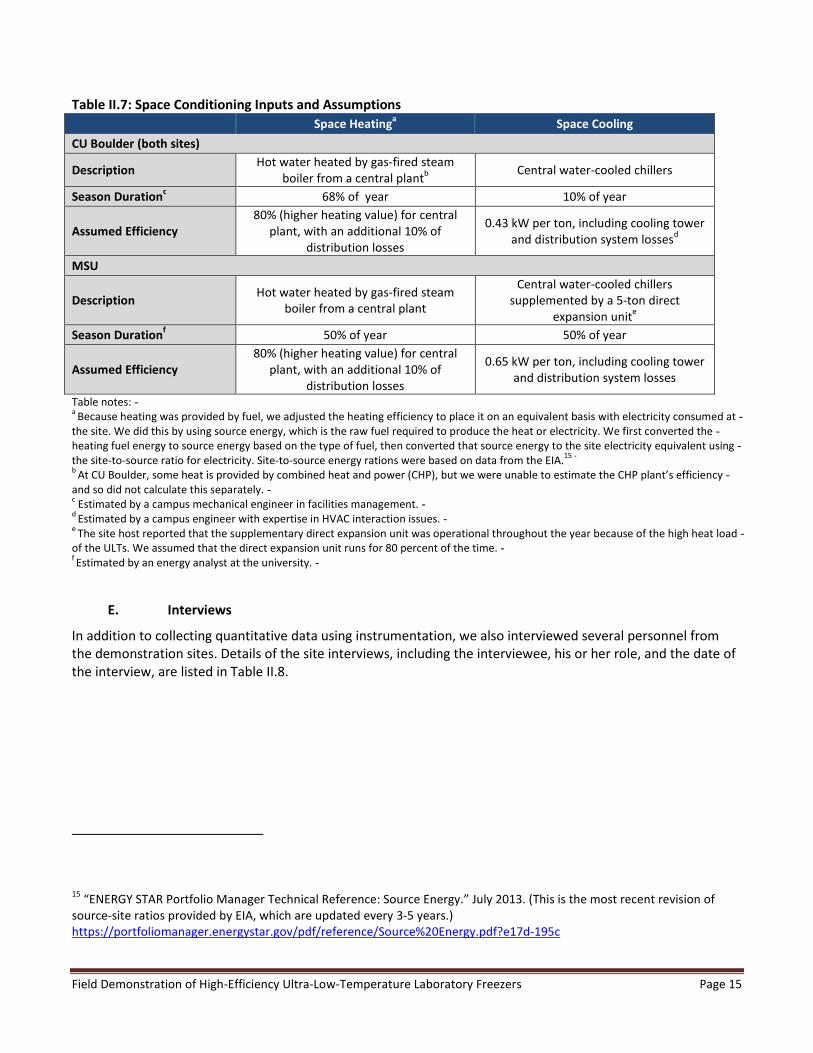

0
200
400
600
800
1000
1200
Demo-1 Demo-2 Demo-3 Average Comparison
Ave
rage
Da
ily
En
erg
y U
se p
er
Cu
bic
Fo
ot
of
Vo
lum
e I
ncl
ud
ing
Po
we
r Fa
cto
r
(VA
-hd
ay
ft3
)
Daily Energy Use at Standardized Conditions
Set-point -80 degC External temp 22 degC Door opening time 30 seconds per day
Figure III3 Adjusted Electricity Consumption for Demo and Average Comparison ULTs Accounting for Power
Factor Not including secondary space conditioning impacts
D Internal Temperature v Set-Point
As discussed in section IIC we independently measured each unitrsquos internal temperature using a calibrated
type-T thermocouple (TC) We observed several cases where the measured temperature differed significantly
from the set-point without a clear cause Table III3 shows the average daily temperature difference from the
set-point and the maximum daily temperature difference from the set-point for each ULT (excluding days during
which the ULT was open for a long period of time ie more than 5 minutes)
Field Demonstration of High-Efficiency Ultra-Low-Temperature Laboratory Freezers Page 20
- deg
- deg
Table III3 Observed Differences between Set-Point and Measured Temperature
Unit Average Deviation from
Set Point ( C)
Maximum Deviation
from Set Point ( C)
Demo-1 76 (warmer) 158 (warmer)
Demo-2 02 (warmer) 84 (colder)
Demo-3 14 (colder) 27 (colder)
Comp-1 65 (warmer) 137 (warmer)
Comp-2 35 (colder) 84 (colder)
Comp-3 21 (warmer) 26 (warmer)
Comp-4 Inconclusive
Average and maximum values represent daily averages ldquoWarmerrdquo indicates the measured temperature was warmer than the set-pointshywhile ldquocolderrdquo indicates the measured temperature was colder than the set-point Data points were excluded if they occurred during ashyday when the set-point was changed a day when the door was open for more than 5 minutes or a day on which we believed there to beshya measurement failure (eg if the TC was accidentally displaced into an ambient environment)shyIn this ULT the TC was displaced for a significant proportion of the measurement period and so we could not draw conclusions aboutshymeasured internal temperature See unadjusted data in Appendix A Figure A13shy
These figures are based on internal temperature measurements taken at one or two locations within each ULT
and are not intended to represent a ldquotruerdquo or average internal temperature of the ULT A determination of a
true average internal temperature would require a ldquomaprdquo of temperature measurement devices which was not
feasible in the context of a field study Due to space constraints we were not able to place the TC in the same
place in each ULT we measured Figure C5 in Appendix C illustrates the relative elevation of our TC within each
ULT
Figure III4 compares the ULTs in the study with the set-point of each ULT adjusted according to the average
deviation from the set-point shown in Table III3 so that the average internal temperature would be expected to
equal -80 degC For example we calculated ULT Comp-1rsquos energy use at a -865 degC set-point assuming that the
average internal temperature is 65 degC warmer than the set-point and would therefore be -80 degC at this
condition Likewise we calculated ULT Demo-3rsquos energy use at a -786 degC set-point assuming that the average
internal temperature is 14 degC colder than the set-point and would therefore be -80 degC at this condition The
results of this exercise suggest that the differences we observed between set-point and measured temperature
do not ultimately change the finding that the demonstration ULTs achieve energy savings over the comparison
ULTs
Field Demonstration of High-Efficiency Ultra-Low-Temperature Laboratory Freezers Page 21
0
100
200
300
400
500
600
700
800
900
Demo-1 Demo-2 Demo-3 Average Comparison
Ave
rag
e D
ail
y E
ne
rgy
Use
pe
r C
ub
ic F
oo
t o
f V
olu
me
(W
-hd
ay
ft3
)
Daily Energy Use at Standardized Conditions
Set-point Calibrated to -80 degC Internal temp External temp 22 degC Door opening
time 90 seconds per day
Figure III4 Adjusted Electricity Consumption for Demo and Average Comparison ULTs Calibrating Set-Point
to Internal Temperature of -80 degC Not including secondary space conditioning impacts
The average daily data do not reflect changes in internal temperature on a minute-to-minute or hour-to-hour
basis For most of the ULTs in the study the measured internal temperature cycled up and down slightly over
time as the compressors in the cascaded refrigeration system turned on and off to maintain the set-point One
exception was the Demo-1 ULT which utilized a Stirling cooler that did not cycle Figure III5 compares the
measured internal temperature for a cascaded-cycle ULT and a Stirling-cycle ULT over the course of a day
Field Demonstration of High-Efficiency Ultra-Low-Temperature Laboratory Freezers Page 22
-60
2000
Temperature Measurements at 1-Minute Intervals of Comp-1 and
Demo-1 ULTs on Example Day (June 29 2013)
Comp-1
Cascade Cycle
Demo-1
Stirling Cycle
000 400 800 1200 1600
-65
Me
asu
red
In
tern
al T
em
pe
ratu
re (
C)
-70
-75
-80
-85
-90
Hours Elapsed
Figure III5 Comparing Internal Temperature of Cascade and Stirling Cycle ULTs
E Interview Findings
Interviews held at each site helped shed light on some qualitative factors that could affect market uptake of
high-efficiency ULTs including purchasing methods operational issues and feedback on the particular ULTs in
the study Section IIE includes a list of interviewees and their roles
Interviewees generally noted that energy efficiency was a factor in the labrsquos ULT purchase decisions though not
the only one or necessarily the most important One said that most labs would incorporate efficiency into their
decision and would potentially pay up to $1000 more for a high-efficiency ULT Another said that the purchasing
department solicited bids and usually chose the lowest one but was starting to look at total cost of ownership
Lab-specific needs can also play a role one interviewee noted that their new demo ULT was more space-
efficient due to the unusual size and shape of the racks needed to store their samples The interviewee added
that their research is government-funded and that they would have to follow government procurement
guidelines18
18 45 CFR 7444(a)(3)(vi) states that Federal research grant recipients when soliciting goods and services as part of their
research must show a ldquoPreference to the extent practicable and economically feasible for products and services that
Field Demonstration of High-Efficiency Ultra-Low-Temperature Laboratory Freezers Page 23
Both interviewees who were directly involved in purchasing noted that vendor relationships were very
important with labs preferring to work with certain sales representatives or vendors with whom they had a long
history The implication was that labs would consider choosing a high-efficiency model but may be more
comfortable with a vendor or manufacturer representative with whom they had an existing trusted
relationship
Common ULT problems that interviewees identified were most often related to operational issues and
maintenance ndash factors that could affect both high-efficiency and typical products equally These problems
included dirty air filters frost buildup or users leaving the door open along with electrical issues like power
outages One person involved in maintenance said that electronics are a common failure point implying that
more electronically-complex ULTs may be more prone to failure Two respondents noted ULT compressors were
a common failure point and since replacing the compressor is a substantial portion of the freezerrsquos cost the ULT
is typically replaced if the compressor fails Average lifetimes and replacement rates reported by interviewees
varied one noted that ULTs may get replaced after 6 to 8 years if repairs become more expensive than
replacement while another estimated a replacement rate of 10 percent of their ULTs per year implying an
average 10-year lifetime Respondents said that ULTs can have a lifetime of 20 to 25 years with preventative
maintenance and repairs
Users of the ULTs being studied in the demonstration did not report that they experienced significant problems
with the new high-efficiency ULTs (Although some of the interviews took place towards the beginning of the
demonstration we remained in contact with users at the demonstration sites and asked them to report any
problems they encountered with the ULTs) Some encountered usability issues For one ULT users had difficulty
engaging the door latch and in one instance this led to the ULT being left ajar for an extended period of time For
another users were unable to open the door immediately after closing it due to suction created by the rapidly
cooling air (most ULTs have an automatic air vent to equalize pressure this ULT had a manual pressure port
intended to eliminate air infiltration when closed) These issues were addressed primarily by educating the
users Two interviewees who had purchased their demo ULTs said that they would consider purchasing that
model again (The third demo ULT was on loan from the manufacturer and the demonstration site operator did
not intend to purchase it at the time of this report writing due to its high cost)
F Economic Analysis
As discussed in the interview findings first cost is a significant factor for purchasers of ULTs Generally the demo
ULTs were more expensive initially than average ULTs with similar qualities (internal volume configuration etc)
We conducted a simple payback analysis to compare the first-cost premium of the demo ULTs to their electricity
cost savings over time not including secondary space-conditioning effects (which would have required a full fuel
cost analysis due to the different fuels used in space heating) or power factor (which is not always accounted for
in utility billing) We obtained list prices for the demo ULTs either directly from manufacturers or from
manufacturer and distributor websites To estimate the price premium associated with the demo ULTs we first
collected list price data for a sample of other ULTs available on the market (including but not limited to the
conserve natural resources and protect the environment and are energy efficientrdquo However this provision is neither well
known nor consistently enforced
Field Demonstration of High-Efficiency Ultra-Low-Temperature Laboratory Freezers Page 24
comparison ULTs measured in the study) from manufacturer and distributor websites We then plotted the data
and developed a linear equation relating list price to volume for this sample of ULTs In this way we could
compare the demo ULTs to a ldquotypicalrdquo ULT of the same volume to avoid biasing the comparison towards smaller
or larger ULTs Figure III6 shows list prices for the demo and other ULTs including the trend-line relating list
price to volume
$25000
$20000 Demo ULTs
$15000 Other ULTs
$10000 Relationship between
Cabinet Volume and List $5000 Price (Other ULTs)
$0
0 40
Figure III6 List Price Data for Demo Models and Other ULTs We obtained list price data from manufacturers and through manufacturer and distributor websites accessed March 2014 ldquoOther
ULTsrdquo includes comparison ULTs in the study as well as other similar models
Purchasers and users of ULTs noted in interviews that ULTs are typically sold through distribution networks and
distributors often offer discounts either on the price of the ULT itself or on accessories such as sample storage
racks or shipping For this reason the difference in list price may not be an accurate representation of the
actual cost difference between the demo ULTs and other ULTs Therefore we included a simple-payback-period
analysis for a full-list-price scenario and a scenario in which the demo ULT and another typical ULT of the same
volume are each discounted by 30 percent However available discounts will vary depending on many factors
so this scenario does not necessarily represent what a given purchaser can expect to pay for a given ULT
In determining electricity savings of each demo ULT compared to a typical ULT we applied the daily energy use
per cubic foot results in Figure III1 and multiplied by the volume of the demo ULT We also considered the
effect of electricity prices on the payback period using EIA data on commercial electricity rates for January
2014 the most recent dataset available at the time of this report19 We calculated the simple payback at three
different commercial electricity rates the US average rate and the highest and lowest rates in the 48
List
Pri
ce
List Price = $320ft3 times Volume + $7459
10 20 30
Internal Cabinet Volume (ft3)
19 US Energy Information Administration Electric Power Monthly with Data for January 2014 published March 2014
httpwwweiagovelectricitymonthlycurrent_yearmarch2014pdf
Field Demonstration of High-Efficiency Ultra-Low-Temperature Laboratory Freezers Page 25
contiguous United States in January 2014 We did not account for other lifetime costs such as maintenance
costs as we did not have any evidence on which to base estimates of these values
Table III4 presents the results of the simple payback analysis for each demo ULT under the two first-cost
scenarios (list price and discounted) and the three electricity rates The simple payback period represents the
time it would take a user to recoup the first cost difference between a demo ULT and a typical ULT
Table III4 Simple Payback Analysis for Demo ULTs
ULT
Model
Average Daily
Energy Savings of
Demo ULT (kWh)a
First Cost
Premium
($)b
Simple Payback Period (years)
High Elec Rate
($01637kWh)c
US Average Rate
($01034kWh)
Low Elec Rate
($00726kWh)
List Price Scenario
Demo-1 15 $2200 25 39 55
Demo-2 48 $2000 70 11 16
Demo-3 44 $3500 13 21 30
30 Discount Scenariod
Demo-1 15 $1600 18 28 40
Demo-2 48 $1400 49 77 11
Demo-3 44 $2500 95 15 21
Table notesshya
Calculated by finding the difference in energy use per cubic foot between each demo ULT and the average of the comparison ULTs asshyshown in Figure III1 and multiplying by the internal volume in cubic feet of the demo ULTshyb
Based on list price data for demo ULTs and linear formula for price per cubic foot of other ULTs Data in Figure III6 Rounded to nearest
$100 c
Source Commercial electricity rates in January 2014 published by EIA20
High and low rates represent the highest and lowest state
commercial electricity rates in the 48 contiguous United States d
Assumes that the same percent discount would be available on both the demo ULTs and average ULTs
IV Summary Findings and Recommendations
A Overall Technology Assessment at Demonstration Facilities
The results of the demonstration support the hypothesis that the demo ULTs can achieve energy savings under
field conditions Over the course of the study the demo ULTs used between 20 percent and 66 percent less
electricity than the average of the comparison ULTs on a per-cubic foot basis and when energy use data were
adjusted to the same operating conditions On an annualized basis users of the demo ULTs would expect to
save between 16 and 55 MWh over the average comparison ULT with an associated cost savings of between
$170 and $570 per year21 (This figure does not include secondary space conditioning impacts which are
expected to vary by location)
20 Ibidshy
21 Assuming an electricity price of $01034kWh the average US electricity rate in the 12-month period ending Januaryshy
2014 according to EIAshy
Field Demonstration of High-Efficiency Ultra-Low-Temperature Laboratory Freezers Page 26
A simple payback analysis discussed in section IIIF suggests that users can recoup the first-cost investment in a
demo ULT within 10 years for certain available discounts and electric rates and assuming that the energy use of
the comparison ULTs is representative of a typical ULT on the market The analysis showed unit Demo-1
recouping its first-cost premium within six years even under the lowest electricity rate assumption In
interviews users estimated freezer lifetimes of between six and 25 years depending on whether the equipment
is maintained and repaired as needed (see section IIIE for interview details) (Actual payback period depends on
circumstances such as first cost differences maintenance and repair costs utility incentives and electricity
prices over the life of the ULT)
Items we were not able to address in this demonstration include long-term reliability whole-cabinet
temperature performance and evaluation of a wider range of ULTs
bull Reliability Over the course of the demonstration we did not observe significant adverse functional
differences among the ULTs included in the study and users of the ULTs did not report any major issues
in using either the demo ULTs or comparison ULTs However given the relatively short demonstration
period we were not able to draw any conclusions about the long-term reliability of the products
bull Whole-cabinet temperature performance We compared a single internal temperature measurement
point to each ULTrsquos set-point with results in section IIID However we were not able to draw firm
conclusions about the temperature performance of the ULTs because gathering the necessary data to
conduct a performance study was not feasible within the scope of the project
bull Range of products covered This report covered a very small sample size of products with the goal of
informing readers of the opportunity presented by high-efficiency ULTs rather than providing definitive
figures for ULT energy use The energy savings observed in this study may not be experienced by all
users due to variation among ULTs and operating conditions Additionally the demo ULTs covered in this
study are not necessarily the only ldquohigh-efficiencyrdquo ULTs on the market and the comparison ULTs may
not represent a truly ldquotypicalrdquo ULT
B Recommendations
Recommendations for ULT Purchasers and Purchasing Organizations
Many users of ULTs experience barriers to purchasing high-efficiency equipment at a cost premium when the
purchaser of the ULT does not pay the electricity cost and thus would not see the energy cost savings from a
more-efficient product This is often the case for universities for example where ULTs are purchased by
individual researchers but energy costs are borne by the university as a whole Given the results of this demo
which suggest favorable payback periods for high-efficiency products we recommend that organizations in this
situation implement formal programs that provide incentives commensurate with the expected savings to
encourage the purchase of efficient products One example is CU Boulderrsquos Green Labs program where the
university ldquopays forwardrdquo the operating cost savings in the form of rebates to researchers who purchase
efficient laboratory equipment based on the expected 3-year electricity cost savings22 Additionally some state
and municipal utilities offer custom rebates and incentives for installing energy-saving equipment23 If relevant
we recommend that customers apply for utility rebates to offset the first-cost of high-efficiency ULTs
22 Discussion with Dr Kathryn Ramirez-Aguilar Green Labs Coordinator at CU Bouldershy
23 For example httpwwwpgecomenmybusinesssaverebatesiefindexpageWTmc_id=Vanity_crshy
Field Demonstration of High-Efficiency Ultra-Low-Temperature Laboratory Freezers Page 27
Interviewees cited the importance of existing vendor relationships as a factor that sometimes prevents
purchasers from procuring new more efficient products We recommend that purchasers communicate to
suppliers that energy efficiency is a factor in purchasing decisions and demonstrate market demand for high-
efficiency equipment by asking for such equipment from their existing vendors and distributors Customers may
also need to develop new vendor relationships to buy more efficient products as long as warranty terms are
acceptable
Recommendations for Manufacturers
We recommend that manufacturers continue to develop and promote high-efficiency products however they
should not compromise reliability in order to do so as reliability is an extremely important factor to ULT users
For new products that customers are unfamiliar with additional marketing and reliability data may be needed to
promote the products We also recommend that manufacturers help support existing efforts being undertaken
by ENERGY STARreg the Better Buildings Alliance the International Institute for Sustainable Labs and other
programs
Recommendations for DOE
DOE is uniquely positioned to aid in deployment of high-efficiency ULTs through the Better Buildings Alliance
Recommendations for promoting adoption of high-efficiency products include
bull Standardization Promote the use of the standardized rating method that DOE and EPA recently
developed through the ENERGY STAR program When used by manufacturers as the basis for rating their
products the rating method can make it easier for potential purchasers of ULTs to identify high-
efficiency products
bull Education Help purchasers overcome first-cost barriers by educating purchasers on life-cycle cost
bull Guidelines Publicize government procurement guidelines that require Federal Agencies and recipients
of government-funded research grants to procure ldquoproductshellip[that] are energy efficientrdquo where
economically feasible and expand these guidelines to other sources of government funding Require
ENERGY STAR ULTs when available
Field Demonstration of High-Efficiency Ultra-Low-Temperature Laboratory Freezers Page 28
V References
Capehart B Turner W and Kennedy W Guide to Energy Management 7th Edition The Fairmont Press 2012
Gumapas Leo Angelo amp Simons Glenn (2013) ldquoFactors affecting the performance energy consumption and
carbon footprint for ultra low temperature freezers case study at the National Institutes of Healthrdquo World
Review of Science Technology and Sustainable Development Vol10 No123 pp129 ndash 141
International Institute for Sustainable Laboratories Annual Conference lthttpi2slorgconferenceindexhtmlgt
Last accessed May 9 2014
Labs for the 21st Century Energy Efficient Laboratory Wiki
lthttplabs21lblgovwikiequipmentindexphpEnergy_Efficient_Laboratory_Equipment_Wikigt Last accessed
May 9 2014
Lane Neill (2013) ldquoUltra-Low Temperature Free-Piston Stirling Engine Freezersrdquo
lthttpwwwstirlingultracoldcomlibsitefileswhitepaper10354-GLOBAL-whitepaper-apr13-vF-webpdfgt Last
accessed May 9 2014
Michigan State University Pharmacology and Toxicology
lthttpwwwphmtoxmsueduresearchindexhtmlhtmgt Last accessed May 9 2014
UC Davis Sustainable 2nd Century Take Action Store Smart
lthttpsustainabilityucdaviseduactionconserve_energystore_smarthtmlgt Last accessed May 9 2014
UCSB Sustainability Laboratory Resources Advocates and Teamwork for Sustainability (LabRATS)
lthttpwwwsustainabilityucsbedulabratsgt Last accessed May 9 2014
University of Colorado at Boulder Integrative Physiology
lthttpwwwcoloradoeduintphysaboutindexhtmlgt Last accessed May 9 2014
University of Colorado at Boulder Molecular Cellular and Developmental Biology
lthttpmcdbcoloradoeduindexshtmlgt Last accessed May 9 2014
US Department of Energy Office of Energy Efficiency and Renewable Energy About the Better Buildings
Alliance lt httpwww4eereenergygovallianceaboutgt Last accessed May 9 2014
US Energy Information Administration ldquoAnalysis and representation of Miscellaneous Electric Loads in NEMSrdquo
Prepared for US Energy Information Administration by Navigant Consulting Inc and SAIC December 2013
lthttpwwweiagovanalysisstudiesdemandmiscelectricpdfmiscelectricpdfgt Last accessed May 9 2014
US Energy Information Administration ldquoElectric Power Monthly with Data for January 2014rdquo Published March
2014 lthttpwwweiagovelectricitymonthlycurrent_yearmarch2014pdfgt Last accessed May 9 2014
US Environmental Protection Agency ldquoENERGY STAR Portfolio Manager Technical Reference Source Energyrdquo
lthttpsportfoliomanagerenergystargovpdfreferenceSource20Energypdfe17d-195cgt Last accessed May
9 2014
Field Demonstration of High-Efficiency Ultra-Low-Temperature Laboratory Freezers Page 29
Appendix A Unadjusted Results and Observations
The following exhibits summarize unadjusted empirical data for each unit We collected data for energy use and
temperature at one-minute intervals and collected door opening data each time the door was opened or
closed As discussed in section IID we aggregated the raw data so as to report the total energy use average
internal and external temperature and number and total time of door openings for each ULT over the course of
a day (1200 AM to 1159 PM) The daily results are shown in the charts below with temperature and energy use
data reported on one graph and the door opening data reported on a subsequent graph Besides the
temperature energy and door opening data that we gathered other data were available at certain sites (eg
one laboratory had an independent monitoring system that recorded the room temperature) We present and
label these data on each graph when they are available We numbered certain observations on each graph and
discuss each numbered observation below the graph
Field Demonstration of High-Efficiency Ultra-Low-Temperature Laboratory Freezers Page A-1
Unit Demo-1 Demonstration ULT 1 at CU Boulder ndash MCDB Lab
14000 40
2
1 3
Nu
mb
er
of
Do
or
Op
en
ing
s p
er
Da
y
Da
ily
En
erg
y C
on
sum
pti
on
(W
hd
ay
)
Av
era
ge
Da
ily
Te
mp
era
ture
(d
eg
C)
12000 20 Real Energy (Watt
Hours) 10000 0
Setpoint (C)
8000 -20
Internal Temp (C) 6000 -40
Internal Temp 4000 -60 (second TC) (C)
2000 -80 External Temp
(C) 0 -100
6713 72713 91513 11413
Date
Figure A1 Daily Energy and Temperature Data Unit Demo-1
12 3000
4
Do
or
Op
en
ing
Tim
e p
er
Da
y (
Se
con
ds)
10 2500
Number of Door 8 2000 Openings
6 1500 Total Seconds of
Door Openings 4 1000
2 500
0 0
6713 72713 91513 11413
Date
Figure A2 Daily Door Opening Data Unit Demo-1
Notes
1 The user changed the set-point several times throughout the course of measurement to better evaluate the
effect of set-point on energy use Researchers in the lab used this ULT for temporary storage During times when
the ULT was not being used to store samples the user sometimes changed the set-point to temperatures
outside the usual storage range (eg -60 degC) to observe the effect on the energy use
2 The internal temperature measurement for this ULT was consistently warmer than the set-point and we
observed several shifts in measured internal temperature over the course of the demonstration with no
corresponding change in set-point
3 For part of the measurement period the user placed a second TC (marked as ldquosecond TCrdquo in the Figure A1
legend above) in this ULT (This second TC was the TC we initially placed in the neighboring ldquobaselinerdquo ULT see
Figure II2 in section IIB for a schematic of ULT placement in the room) The user initially placed the second TC
Field Demonstration of High-Efficiency Ultra-Low-Temperature Laboratory Freezers Page A-2
next to the first TC in the top of the ULT for several daysmdash93013 to 10413mdashto confirm the temperature
readings from the original TC (This ULT had three compartmentsmdashin the top middle and bottom See Figure
C5 in Appendix C for a diagram of initial TC placement within each ULT) In this position the second TC
measured a temperature similar to the first TC Then the user moved the second TC to the bottom of the ULT
where it measured a temperature closer to the ULT set-point For one day towards the end of the measurement
periodmdash111713mdashthe user moved the second TC to the middle compartment of the ULT where it also
measured a temperature close to the ULT set-point These temperature checks suggest that the ldquowarmrdquo zone
was confined to the top compartment of the ULT
4 At one point during the monitoring period a user did not fully engage the door latch after accessing the ULT
and the door remained partially open for an extended amount of time The site host communicated to the ULTrsquos
manufacturer that the latch was difficult to close
Field Demonstration of High-Efficiency Ultra-Low-Temperature Laboratory Freezers Page A-3
Unit Comp-1 Comparison ULT 1 at CU Boulder ndash MCDB Lab
-100
-80
-60
-40
-20
0
20
40
0
5000
10000
15000
20000
25000
30000
6713 72713 91513 11413
Av
era
ge
Da
ily
Te
mp
era
ture
(d
eg
C)
Da
ily
En
erg
y C
on
sum
pti
on
(W
hd
ay
)
Date
Real Energy
(Watt Hours)
Setpoint (C)
Internal Temp
(C)
External Temp
(C) 1
2
3
4
Figure A3 Daily Energy and Temperature Data Unit Comp-1
14 600
Do
or
Op
en
ing
Tim
e p
er
Da
y (
Se
con
ds)
Number of Door
Openings
Total Seconds of
Door Openings 200
100
0Nu
mb
er
of
Do
or
Op
en
ing
s p
er
Da
y 12 500
6713 72713 91513 11413
10 400
8
300
6
4
2
0
Date
Figure A4 Daily Door Opening Data Unit Comp-1
Notes
1 We do not know the reason for this sudden drop in daily average measured temperature
2 The user maintained the set-point at -80 degC because the researcher who owned the ULT did not give
permission to change the set-point so we were unable to observe the effect of set-point change on energy use
3 Gaps in internal temperature data correspond to the periods when we moved the thermocouple from this
ULT to the neighboring Demo-1 ULT (see discussion above under Demo-1)
4 The external temperature sensor failed towards the end of the measurement period We did not replace it
because we already had enough data to correlate external temperature with energy use
Field Demonstration of High-Efficiency Ultra-Low-Temperature Laboratory Freezers Page A-4
Unit Demo-2 Demonstration ULT 2 at CU Boulder ndash iPhy Lab
18000 40 D
ail
y E
ne
rgy
Co
nsu
mp
tio
n (
Wh
da
y)
16000 20
Av
era
ge
Da
ily
Te
mp
era
ture
(d
eg
C)
Real Energy 14000 (Watt hours)
0 12000 Setpoint (C)
-20 10000
Internal Temp 8000 -40
(C)
6000 2 -60
1 Internal Temp
(second TC) (C) 4000
-80 External Temp 2000 (C)
0 -100
6713 72713 91513 11413
Date
Figure A5 Daily Energy and Temperature Data Unit Demo-2
0
100
200
300
400
500
600
700
800
900
1000
0
5
10
15
20
25
30
35
Do
or
Op
en
ing
Tim
e p
er
Da
y (
Se
con
ds)
Nu
mb
er
of
Do
or
Op
en
ing
s p
er
Da
y
Number of Door
Openings
Total Seconds of
Door Openings
3
6713 72713 91513 11413
Date
Figure A6 Daily Door Opening Data Unit Demo-2
Notes
1 The user changed the set-point from -80 degC to -70 degC partway through the measurement period to observe the
effect of this change on the ULTrsquos energy use
2 For a short time the user placed a second TC (marked as ldquosecond TCrdquo in the legend) in the ULT (This second
TC was the TC we initially placed in the Comp-2 ULT see Figure II3 in section IIB for a schematic of ULT
placement in the room) The user initially placed the second TC next to the first TC in the top of the ULT for
several daysmdash101113 to 101513mdashto confirm the temperature readings from the first TC Then the user
moved the second TC to the bottom of the ULT for several daysmdash101613 to 102113 The TCs measured
similar temperatures in both places
3 After we initially set up the instrumentation the door opening loggerrsquos adhesive detached from the door
causing the loss of the first two weeks of door-opening data The user observed this and replaced the sensor
Field Demonstration of High-Efficiency Ultra-Low-Temperature Laboratory Freezers Page A-5
Unit Comp-2 Comparison ULT 2 at CU Boulder ndash iPhy Lab
25000 40 N
um
be
r o
f D
oo
r O
pe
nin
gs
pe
r D
ay
D
ail
y E
ne
rgy
Co
nsu
mp
tio
n (
Wh
da
y)
1
3
2shy
Av
era
ge
Da
ily
Te
mp
era
ture
(d
eg
C)
20
0
Real Energy 20000 (Watt hours)
Setpoint (C) 15000
-20
Internal Temp -40
10000 (C)
Internal Temp -60 (second TC) (C) 5000
-80 External Temp
(C) 0 -100shy6713 72713 91513 11413shy
Date
Figure A7 Daily Energy and Temperature Data Unit Comp-2
12 600
Do
or
Op
en
ing
Tim
e p
er
Da
y (
Se
con
ds)
10 500
6713 72713 91513 11413
Number of Door 8 400 Openings
6 300 Total Seconds of
Door Openings 4
2
0
200
100
0
Date
Figure A8 Daily Door Opening Data Unit Comp-2
1 The user changed the set-point from -80 degC to -70 degC partway through the measurement period to observe the
effect on energy use however this did not appear to cause a commensurate change in the measured internal
temperature We do not know why this occurred
2 From 101113 to 102113 the user had placed the TC from this ULT into the adjacent ULT (the Demo-2 ULT
see Figure A5 above) On 102213 through the end of the measurement period the user moved both TCs into
this ULTmdashthe TC initially in this ULT in the bottom and the second TC in the top The TCs measured similar
temperatures
3 The initial TC fell out of the ULT for a short period of time We noticed this in our real-time review of the data
and notified the site host who repositioned it in the cabinet
Field Demonstration of High-Efficiency Ultra-Low-Temperature Laboratory Freezers Page A-6
Unit Demo-3 Demonstration ULT 3 at Michigan State University
-100
-80
-60
-40
-20
0
20
40
0
5000
10000
15000
20000
25000
71013 82913 101813 12713
Av
era
ge
Da
ily
Te
mp
era
ture
(d
eg
C)
Da
ily
En
erg
y C
on
sum
pti
on
(W
hd
ay
)
Date
Real Energy
(Watt hours)
Internal Temp
(C)
Setpoint (C)
External Temp
(C)
Measured Room
Temp (C)
1
23
Figure A9 Daily Energy and Temperature Data Unit Demo-3
30 1200
Nu
mb
er
of
Do
or
Op
en
ing
s p
er
Da
y
Do
or
Op
en
ing
Tim
e p
er
Da
y (
Se
con
ds)
71013 82913 101813 12713
25 1000
20 800 Number of Door
Openings
15 600
10
5
0
Total Seconds of
Door Openings 400
200
0
Date
Figure A10 Daily Door Opening Data Unit Demo-3
Notes
1 The user changed the set-point from -80 degC to -85 degC towards the end of the measurement period to observe
the effect on energy use
2 These supplementary data are from a room air-temperature sensor associated with the building energy
system for which the user provided data for part of the measurement period We present those data as
ldquoMeasured Room Temprdquo alongside the measured external temperature data for comparison
3 The site host reported that the building air conditioning system failed during the time associated with this
temperature spike The impacts on the ULTrsquos energy use (see Real Energy curve) were substantial
Field Demonstration of High-Efficiency Ultra-Low-Temperature Laboratory Freezers Page A-7
Unit Comp-3 Comparison ULT 3 at Michigan State University
30000 40
20
-100
1
23D
ail
y E
ne
rgy
Co
nsu
mp
tio
n (
Wh
da
y)
Av
era
ge D
ail
y T
em
pe
ratu
re (
de
g C
)
Real Energy 25000
20000
(Watt hours)
0 Internal Temp
(C) -20
15000 Setpoint (C) -40
10000 External Temp -60 (C)
5000 -80 Measured Room
Temp (C) 0
71013 82913 101813 12713
Date
Figure A11 Daily Energy and Temperature Data Unit Comp-3
0
50
100
150
200
250
300
350
400
0
2
4
6
8
10
12
14
16
18
20
71013 82913 101813 12713
Do
or
Op
en
ing
Tim
e p
er
Da
y (
Se
con
ds)
Nu
mb
er
of
Do
or
Op
en
ing
s p
er
Da
y
Date
Number of Door
Openings
Total Seconds of
Door Openings
Figure A12 Daily Door Opening Data Unit Comp-3
Notes
1 The user changed the set-point from -80 degC to -85 degC towards the end of the measurement period to observe
the effect on energy use
2 These supplementary data are from a room air-temperature sensor associated with the building energy
system for which the user provided data for part of the measurement period We present those data as
ldquoMeasured Room Temprdquo alongside the measured external temperature data for comparison
3 The site host reported that the building air conditioning system failed during the time associated with this
temperature spike The impacts on the ULTrsquos energy use (see Real Energy curve) were substantial
Field Demonstration of High-Efficiency Ultra-Low-Temperature Laboratory Freezers Page A-8
Unit Comp-4 Comparison ULT 4 at Michigan State University
18000 40
16000 20
3 2 D
ail
y E
ne
rgy
Co
nsu
mp
tio
n (
Wh
da
y)
Ave
rag
e D
ail
y T
em
pe
ratu
re (
de
g C
)
Real Energy
(Watt hours)
Internal Temp
(C)
Setpoint (C)
External Temp
(C)
Measured Room
Temp (C)
14000 0
12000
-20 10000
8000 -40 4 5shy
-60 4000
6000
-80 2000
1 0 -100
71013 82913 101813 12713 Date
Figure A13 Daily Energy and Temperature Data Unit Comp-4
0
200
400
600
800
1000
1200
0
5
10
15
20
25
30
35
40
45
50
71013 82913 101813 12713
Do
or
Op
en
ing
Tim
e p
er
Da
y (
Se
con
ds)
Nu
mb
er
of
Do
or
Op
en
ing
s p
er
Da
y
Date
Number of Door
Openings
Total Seconds of
Door Openings
Figure A14 Daily Door Opening Data Unit Comp-4
Notes
1 The user changed the set-point from -80 degC to -85 degC towards the end of the measurement period to observe
the effect on energy use
2 These supplementary data are from a room air-temperature sensor associated with the building energy
system for which the user provided data for part of the measurement period We present those data as
ldquoMeasured Room Temprdquo alongside the measured external temperature data for comparison
3 The site host reported that the building air conditioning system failed during the time associated with this
temperature spike The impacts on the ULTrsquos energy use (see Real Energy curve) were substantial
4 On 81713 the site host reported that the cover on the internal temperature sensor was missing (see
Appendix C for a description of the temperature sensor setup) The site host did not report whether the sensor
Field Demonstration of High-Efficiency Ultra-Low-Temperature Laboratory Freezers Page A-9
was in its original position or whether it had been dislodged however these factors may explain the change in
measured temperature for several days prior to this date Upon replacing the cover and repositioning the
probe temperature measurements returned to the range initially measured
5 On 112713 the site host reported finding the thermocouple up against the inner door and moved it back
into the shelf space We observed that for several weeks prior to this date the temperature that the TC
measured was higher than the set-point which also corresponded to a reduction in the ULTrsquos energy use We do
not know why energy use dropped during this period
Field Demonstration of High-Efficiency Ultra-Low-Temperature Laboratory Freezers Page A-10
Appendix B Regression Analysis Methodology and Results
After aggregating the data on a daily basis as presented in the figures in Appendix A we conducted a regression
analysis to determine the effect of certain variables on the energy use of each ULT The variables we examined
were the ULTrsquos set-point the measured ambient temperature and the total time the ULTrsquos outer door was
opened each day We used the results of this analysis to develop equations expressing the expected energy use
in terms of these variables to compare performance of the ULTs at a common set of operating conditions The
following paragraphs discuss the choice of variables
Internal Temperature or Set-point
We initially planned to correlate the energy use to the measured internal temperature However after a review
of the data we determined that set-point would be a more appropriate variable for several reasons First it
was unclear whether our measured internal temperature was more representative of average cabinet
temperature than the ULTrsquos own internal temperature sensor (which we assumed to be the input to the
temperature control to meet the set-point) In some cases it appears that neither the set-point nor the
measured internal temperature provided a true reflection of the average cabinet temperature For three of the
ULTs we were able to place two temperature sensors in different areas of the ULT for short periods of time but
in one of these cases the two sensors did not measure consistent temperatures (See Figure A1 Figure A5
and Figure A7) Second the set-point was not dependent on the other variables while the internal temperature
could be affected by door openings Third the set-point seemed to be a more salient predictor of the energy use
than the measured internal temperature For example in Figure A7 a 10-degree change in the set-point is
correlated with an observable drop in energy use even though the measured internal temperature did not
appear to change significantly In another example the temperature and energy data in Figure A13 show a
correlation between higher internal temperature and lower energy use absent a change in set-point However
the data do not indicate if one is causing the other or whether some other factor is causing both changes For
these reasons we chose set-point as the regression variable The relationship between set-point and average
internal temperature is certainly of interest and may warrant further study (we believe such study would be
more appropriate in a test laboratory setting rather than a field setting) however as discussed we could not
draw firm conclusions using the data collected in this demonstration
External Temperature
In the regression analysis we also correlated the energy use to the ULTrsquos ambient-air temperature (measured at
the condenser inlet) We observed in the unadjusted daily data that higher ambient-air temperature is
associated with greater energy use (see Figure A9 Figure A11 and Figure A13) Although door openings often
caused a temporary drop in the external temperature when viewed at 1-minute intervals due to the placement
of the temperature probe below the door the door openings did not noticeably affect the average daily external
temperature Therefore we assumed that the average daily external temperature was independent from other
variables with respect to its effect on energy use
Door Openings
As noted in Appendix A we aggregated on a daily basis both the number of door openings and the total time a
door was open We chose the total time a door was open for the regression analysis We expected this to
correlate somewhat more strongly with energy use (compared to the number of door openings) because it more
closely reflects the amount of heat entering the ULT
Field Demonstration of High-Efficiency Ultra-Low-Temperature Laboratory Freezers Page B-11
Analysis
The outcome of the analysis was an equation in the following form
Energy Use = A times Set-point + B times External Temperature + C times Door Opening Seconds + Intercept
Where coefficients A B C and the Y-intercept were determined for each ULT by the regression analysis We
assumed that the three variables were not directly related to each other which we believe is a valid assumption
based on the previous paragraphs Prior to the regression analysis we removed outlying data that did not reflect
normal ULT use either due to user error (eg leaving the door open as shown in Figure A2) or instrumentation
error (eg sensor displacement as shown in Figure A7 or sensor failure as shown in Figure A3) To fairly
compare the ULTs we chose a set of standardized conditions to apply in the regression equation The
standardized conditions represented average conditions experienced by the ULTs in aggregate as observed in
the demonstration data and are as follows
Table B-1 Conditions for Calculating Standardized Energy Use
Condition Value
Setpoint (degC) -80
External Temperature (degC) 22
Door opening seconds 90
The following charts and tables show the results of the regression analysis for each ULT in the demomdashthat is
how each ULTrsquos energy use is predicted to scale with set-point external temperature and door opening time
expressed as coefficients A B and C in the regression equation respectively and the intercept of the equation
We also present the expected energy use at the standardized conditions from Table B-1 and the estimation
error associated with each variable in the analysis The error is a measure of confidence in the results there is a
95 percent probability that the true result lies within the error bounds
Following each table a chart compares the expected energy use of the ULT at the standardized conditions to
the measured energy use with the estimation error shown as a shaded band The band represents the range of
predicted energy use at the given conditions when we accounted for the statistical error
The results comparing each ULT at the standardized conditions are shown in section IIIA
Field Demonstration of High-Efficiency Ultra-Low-Temperature Laboratory Freezers Page B-12
Unit Demo-1 Demonstration ULT 1 at CU Boulder ndash MCDB Lab
Table B-2 Regression Variables and Standardized Energy Use Unit Demo-1
Coefficient Variable Value Error
Intercept Constant (Wh) -3733 1427
A Setpoint (WhdegC) -140 8
B External Temperature (WhdegC) 14 58
C Door opening seconds (Whs) 148 016
Total Daily Energy Use (Wh) 7851 2060
Da
ily
En
erg
y C
on
sum
pti
on
(W
hd
ay)
14000
12000
10000 Standardized Energy
Use Error 8000
Standardized Energy 6000 Use
Measured Daily 4000
Energy Useshy
2000shy
0
61213 71213 81213 91213 101213 111213
Date
Figure B1 Unadjusted Measured Daily Energy Use v Standardized Daily Energy Use Unit Demo-1
Field Demonstration of High-Efficiency Ultra-Low-Temperature Laboratory Freezers Page B-13
Unit Comp-1 Comparison ULT 1 at CU Boulder ndash MCDB Lab
Table B-3 Regression Variables and Standardized Energy Use Unit Comp-1
Coefficient Variable Value Error
Intercept Constant (Wh) 16163 781
A Setpoint (WhdegC) 0 0
B External Temperature (WhdegC) 316 41
C Door opening seconds (Whs) 429 071
Total Standardized Daily Energy Use (Wh) 23248 1696 Setpoint was not changed during the evaluation period therefore there was no basis on which to correlate set-point with energy use
for this ULT
30000shy
25000shy
20000shy
Standardized Energy 15000 Use Error
Standardized Energy 10000
Use
Measured Daily 5000 Energy Use
0
Da
ily
En
erg
y C
on
sum
pti
on
(W
hd
ay
)
61213 71213 81213 91213 101213 111213
Date
Figure B2 Unadjusted Measured Daily Energy Use v Standardized Daily Energy Use Unit Comp-1
Field Demonstration of High-Efficiency Ultra-Low-Temperature Laboratory Freezers Page B-14
Unit Demo-2 Demonstration ULT 2 at CU Boulder ndash iPhy Lab
Table B-4 Regression Variables and Standardized Energy Use Unit Demo-2
Coefficient Variable Value Error
Intercept Constant (Wh) -19994 571
A Setpoint (WhdegC) -313 4
B External Temperature (WhdegC) 311 19
C Door opening seconds (Whs) 292 011
Total Standardized Daily Energy Use (Wh) 12006 668
Da
ily
En
erg
y C
on
sum
pti
on
(W
hd
ay
)
18000
16000
14000
12000
10000 Standardized Energy
Use Error 8000
Standardized Energy 6000
Useshy4000shy
Measured Dailyshy2000shy Energy Use
0
61813 71813 81813 91813 101813 111813
Date
Figure B3 Unadjusted Measured Daily Energy Use v Standardized Daily Energy Use Unit Demo-2
Field Demonstration of High-Efficiency Ultra-Low-Temperature Laboratory Freezers Page B-15
Unit Comp-2 Comparison ULT 2 at CU Boulder ndash iPhy Lab
Table B-5 Regression Variables and Standardized Energy Use Unit Comp-2
Coefficient Variable Value Error
Intercept Constant (Wh) -7905 450
A Setpoint (WhdegC) -267 4
B External Temperature (WhdegC) 216 13
C Door opening seconds (Whs) 424 021
Total Standardized Daily Energy Use (Wh) 18336 436
Da
ily
En
erg
y C
on
sum
pti
on
(W
hd
ay)
0
5000
10000
15000
20000
25000
61813 71813 81813 91813 101813 111813
Standardized Energy
Use Error
Standardized Energy
Use
Measured Daily
Energy Use
Date
Figure B4 Unadjusted Measured Daily Energy Use v Standardized Daily Energy Use Unit Comp-2
Field Demonstration of High-Efficiency Ultra-Low-Temperature Laboratory Freezers Page B-16
Unit Demo-3 Demonstration ULT 3 at Michigan State University
Table B-6 Regression Variables and Standardized Energy Use Unit Demo-3
Coefficient Variable Value Error
Intercept Constant (Wh) -43938 1635
A Setpoint (WhdegC) -737 17
B External Temperature (WhdegC) 96 28
C Door opening seconds (Whs) 311 014
Total Standardized Daily Energy Use (Wh) 17233 858
Da
ily
En
erg
y C
on
sum
pti
on
(W
hd
ay)
25000
20000
15000 Standardized Energy
Use Error
10000 Standardized Energy
Use
5000 Measured Daily
Energy Use
0
71213 81213 91213 101213 111213
Date
Figure B5 Unadjusted Measured Daily Energy Use v Standardized Daily Energy Use Unit Demo-3
Field Demonstration of High-Efficiency Ultra-Low-Temperature Laboratory Freezers Page B-17
Unit Comp-3 Comparison ULT 3 at Michigan State University
Table B-7 Regression Variables and Standardized Energy Use Unit Comp-3
Coefficient Variable Value Error
Intercept Constant (Wh) -62157 1872
A Setpoint (WhdegC) -949 19
B External Temperature (WhdegC) 245 34
C Door opening seconds (Whs) 401 033
Total Standardized Daily Energy Use (Wh) 19293 1138
Da
ily
En
erg
y C
on
sum
pti
on
(W
hd
ay
)
30000
25000
20000 Standardized Energy
Use Error 15000
Standardized Energy
Use 10000
Measured Daily
Energy Use 5000shy
0shy71213 81213 91213 101213 111213
Date
Figure B6 Unadjusted Measured Daily Energy Use v Standardized Daily Energy Use Unit Comp-3
Field Demonstration of High-Efficiency Ultra-Low-Temperature Laboratory Freezers Page B-18
Unit Comp-4 Comparison ULT 4 at Michigan State University
Table B-8 Regression Variables and Standardized Energy Use Unit Comp-4
Coefficient Variable Value Error
Intercept Constant (Wh) -16974 3349
A Setpoint (WhdegC) -154 36
B External Temperature (WhdegC) 762 64
C Door opening seconds (Whs) 223 042
Total Standardized Daily Energy Use (Wh) 12205 1918
Da
ily
En
erg
y C
on
sum
pti
on
(W
hd
ay
)
18000
16000
14000
12000
10000 Standardized Energy
Use Error 8000
Standardized Energy 6000
Useshy4000shy
Measured Dailyshy2000shy Energy Use
0
71213 81213 91213 101213 111213
Date
Figure B7 Unadjusted Measured Daily Energy Use v Standardized Daily Energy Use Unit Comp-4
Field Demonstration of High-Efficiency Ultra-Low-Temperature Laboratory Freezers Page B-19
Appendix C Instrumentation and Data Collection Details
Energy
We measured real energy (watt hours) amp hours and reactive energy (volt-amp reactive (VAR) hours) for each
ULT at one-minute intervals using a Veris T-VER-E50B2 Compact Power and Energy Meter sold by Onset
Computer Corporation (Onset) The measurement accuracy was 05 for real power 2 for reactive power and
between 04 and 08 for current depending on the surrounding air temperature27
The inputs to the power meter were the current and three-phase voltage (in addition to control power to drive
the meter) Because the power supplied to the ULTs was in a 3-wire configuration the wires had to be isolated
from each other to measure the current and voltage A qualified electrician wired each meter in an electrical box
that the ULT could plug into The wires were isolated inside the box in a touch-safe configuration and an
electrical cord connected the box to the wall outlet Figure C1 and Figure C2 show the wiring diagrams for
boxes connected to ULTs with NEMA 5-20 (line-neutral-ground) and NEMA 6-15 (line-line-ground) electrical
cords respectively Figure C3 shows a photograph of the setup of the power meter inside the electrical box
27 Onset Computer Corporation T-VER-E50B2 Compact Power and Energy Meter Installation Guide
Field Demonstration of High-Efficiency Ultra-Low-Temperature Laboratory Freezers Page C-20
Figure C1 Electrical Diagram for NEMA 5-20 Connector
Field Demonstration of High-Efficiency Ultra-Low-Temperature Laboratory Freezers Page C-21shy
Figure C2 Electrical Diagram for NEMA 6-15 Connector
Field Demonstration of High-Efficiency Ultra-Low-Temperature Laboratory Freezers Page C-22shy
Outputs from meter Inputs from CT to meter (left to right A-h W-h VAR-h)
Fuses
Power
meter
Inputs
from line
to meter
Current
transformer
Power line from Outlet for ULT wall outlet
Figure C3 Photograph of Power Meter Inside Electrical Box
The output of the power meter consisted of three separate signals for energy amp hours and VAR hours The
three signals were transmitted to the data logger using Onset HOBO S-UCC-M00x electronic switch pulse input
adapters (the ldquoxrdquo in the model number corresponds to the length of the cable) which adapted the signal to a
smart-sensor input to the logger28 Figure C4 shows a picture of a pulse input adapter and cable
Photo credit Dave Trumpie
28 Onset Computer Corporation Pulse Input Adapters for use with HOBO H21 H22 and U30 Series Data Loggers
Field Demonstration of High-Efficiency Ultra-Low-Temperature Laboratory Freezers Page C-23
Source Onset Computer Corporation
Figure C4 Pulse Input Adapter and Cable from Power Meter to Logger
We measured both real energy and reactive energy to determine the power factor of each ULT Power factor
relates the ldquorealrdquo power that performs useful work (ie refrigeration ) to the ldquoreactiverdquo power associated with
the magnetizing current used to operate inductive devices (ie compressors) A high power factor means that
most of the electrical power supplied by the circuit is being used for real work A low power factor on the other
hand means that most of the total power becomes inductive losses Appendix D provides a tutorial for
calculating power factor given the real and reactive power
Power factor is important because while customers are often billed only for the real power used by a device
the electrical circuit containing the device must be sized for and the utility must provide the total power Thus
utilities sometimes impose a separate ldquopower factorrdquo cost that penalizes industrial customers using low power
factor devices29 Power factor for the ULTs in the demonstration is reported in section IIIC
Internal Temperature
We measured internal temperature at one-minute intervals using Type T thermocouples The limit of error for
the thermocouples was 10 degC or 15 at temperatures below 0 degC whichever is greater30 Where possible we
placed each internal thermocouple near the top of the ULT as we assumed this would likely correspond to the
highest cabinet temperature This was not possible for two ULTs due to space constraints (caused by items
stored in the ULT) in these cases we placed the internal thermocouple where space was available Figure C5
shows the approximate elevation of the thermocouples within each ULT Each ULT also had a built-in
temperature sensor used to maintain the ULTrsquos setpoint but we did not know the location of the built-in sensor
for all ULTs and in some cases determining its location would have involved unloading the ULT which would
have disturbed the samples inside We observed that in many cases the temperature measured by the
thermocouple was not the same as the displayed set-point temperature A single-point measurement such as
the measured temperature or the set-point temperature is not a reliable indicator of the average cabinet
temperature however attempting to determine the average cabinet temperature more accurately would have
29 Capehart B Turner W and Kennedy W Guide to Energy Management 7th Edition The Fairmont Press 2012
30 Revised Thermocouple Reference Tables Type T Reference Tables NIST Monograph 175 Revised to ITS-90
Field Demonstration of High-Efficiency Ultra-Low-Temperature Laboratory Freezers Page C-24
required an array of thermocouples which is impractical in a field test because it would interfere with the
normal use of the ULT In Appendix A both the measured temperature and set-point temperature are reported
for all ULTs on a daily basis
Demo-1 Comp-1shy
Demo-2 Comp-2shy
Demo-3 Comp-3 Comp-4shy
Figure C5 Front View of Each ULT Showing Approximate Relative Elevation of Internal ThermocouplePlacement
We embedded each thermocouple in a plastic vial and attached each vial to a small cardboard box The purpose
of this was threefold
1) To protect the tip of the thermocouple from breakageshy2) To provide thermal mass to simulate the temperature of a typical sample inside the ULT andshy
Field Demonstration of High-Efficiency Ultra-Low-Temperature Laboratory Freezers Page C-25
3) To enhance the visibility of the thermocouple to reduce the likelihood that it would be accidentally
damaged or discarded
Figure C6 shows how the thermocouples were attached to the box and has an example photo of placement
within the ULT
(1) Bare thermocouple (2) Thermocouple embedded in vial
(3) Vial attached to box (4) Box placed in ULT (space permitting)
Photo credits (1)-(3) Rebecca Legett (4) Dave Trumpie
Figure C6 Thermocouple Apparatus
We connected the thermocouples to an Omega TX-13 temperature transmitter which converted the
temperature sensed by each thermocouple junction to a 4 to 20 milli-amp (mA) signal The transmitter allowed
scaling of its output to a fixed range of temperatures (-100 to 100 degC) so that given a mA output the
temperature corresponding to that output could be easily determined In other words an output of 4 mA would
correspond to a temperature of -100 degC and an output of 20 mA would correspond to a temperature of 100 degC
For outputs between 4 and 20 mA the temperature is determined through linear interpolation as
recommended by the instrumentation manufacturer31
31 Omega Engineering Inc Userrsquos Guide TX13 Push Button Thermocouple
Field Demonstration of High-Efficiency Ultra-Low-Temperature Laboratory Freezers Page C-26
We connected the temperature transmitter to the analog input to the data logger using twisted pair cable also
recommended by the manufacturer
Thermocouple
Wire Input
Twisted Pair Cable
Output
Photo credit Dave Trumpie
Figure C7 Photo of Temperature Transmitter
Each thermocouple-transmitter pair was calibrated to -60 -70 and -80 degC by Transcat Calibration amp Compliance
Services We chose these calibration temperatures because they encompassed the likely range of temperatures
that the thermocouple would be measuring
External Temperature
We measured external temperature at one-minute intervals using an Onset S-TMB-M00x 12-Bit Temperature
Smart Sensor whose probe end we placed at the air inlet to the condenser just outside of the grille (The ldquoxrdquo in
the model number refers to the length of the sensor cable in meters we used different lengths in the
demonstration as needed) The manufacturer lists accuracy of the sensor as lt +- 02 degC from 0deg to 50 degC32
Figure C8 shows a photograph of the external temperature probe and its cable and Figure C9 shows example
photographs of the external temperature probe attached to the ULTrsquos air inlet grille
32 Onset Computer Corporation 12-Bit Temperature Smart Sensor Manual
Field Demonstration of High-Efficiency Ultra-Low-Temperature Laboratory Freezers Page C-27
Photo credit Onset Computer Corporation
Figure C8 Temperature Sensor and Cable from Sensor to Logger
Photo credit Dennis Schroeder NREL Photo credit Dave Trumpie
Figure C9 Photos of External Temperature Probe Placement
Energy and Temperature Data Logging
We logged energy and temperature data using an Onset HOBO U30 Station with remote communication
capabilities including GSM (Global System for Mobile Communications in other words cellular phone network
communication) used at the CU Boulder sites and Wi-fi used at the MSU site33 Each U30 station was capable
of receiving input from up to 10 smart sensors and two analog sensors The power meter output adapters and
33 Onset Computer Corporation HOBO U30 Station Userrsquos Guide
Field Demonstration of High-Efficiency Ultra-Low-Temperature Laboratory Freezers Page C-28
the external temperature sensor were smart-sensor inputs with plug-and-play capability The internal
thermocouple was an analog input that required configuration to scale the mA output to the temperature (as
discussed in the previous section) Figure C10 shows a photograph of the data logger with inputs indicated
Analog
Inputs
Photo credit Dennis Schroeder NREL
Smart Sensor Inputs
Figure C10 Diagram of Data Logger Inputs
The number of inputs allowed one logger to be used for either two or three ULTs For the CU Boulder sites we
monitored two ULTs in each room Figure C11 shows a schematic diagram of the sensor inputs to the loggers in
this configuration
Field Demonstration of High-Efficiency Ultra-Low-Temperature Laboratory Freezers Page C-29
Legend
A
D
= Analog sensor (internal temp)shy
= Digital sensor (external temp)shy
Data Logger
Cellular
Signal
ULT 1
D
A
Power
meter
ULT 2
D
A
Power
meter
= Temperature transmitter
= Power supply
= Data connection
Figure C11 Instrumentation Schematic for CU Boulder Sites
At the Michigan State University site there were three ULTs in one room which were some distance away from
each other (see Figure II4 in section IIB) To avoid running multiple long-distance wires we consolidated the
smart sensor inputs into a single cable using a cable consolidator This allowed the signals from multiple sensors
to be transmitted through a single cable Furthermore there were three total analog sensors in the MSU lab but
only two analog ports on the logger We converted one of the analog sensors to a digital ldquosmartrdquo signal input
Field Demonstration of High-Efficiency Ultra-Low-Temperature Laboratory Freezers Page C-30
meter
using an Onset S-CIA-CM14 12-bit 4-20 mA input adapter34 We included a separate 12 VDC power supply to
supply power to that analog sensor Figure C12 shows a diagram of the instrumentation setup at the Michigan
State University site
Legend
A
D
= Analog sensor (internal temp)shy
= Digital sensor (external temp)shy
= Temperature transmitter Wi-fi Signal
Data
Logger
ULT 1 ULT 2 ULT 3
D
A A
D
A
D
Power
meter
Consolidator
box
Power
Consolidator
box
Power
meter
Input adapter
= Power supply
= Data connection
Figure C12 Instrumentation Schematic for Michigan State University Lab
34 Onset Computer Corporation 12-Bit 4-20 mA Input Adapter Manual
Field Demonstration of High-Efficiency Ultra-Low-Temperature Laboratory Freezers Page C-31
Door Openings
We monitored door openings using a stand-alone state logger35 The state logger consisted of a logging device
on the main body of the ULT with a magnetic switch and a magnet attached to the outer door Each time a user
opened the door the magnetic connection would be broken and the logger would record the timestamp Once
the door was closed the logger would sense the magnetic field and record another timestamp Figure C13
shows a schematic diagram of the data logger and magnet while Figure C14 shows a photograph of the logger
attached to a door We calculated the duration of each door opening by subtracting each door-open timestamp
from its subsequent door-closed timestamp
Internal Magnetic Switch
Magnet
Picture credit Onset Computer Corporation
Figure C13 Diagram of Logger and Magnet
35 Onset Computer Corporation HOBO State Data Logger (UX90-001x) Manual
Field Demonstration of High-Efficiency Ultra-Low-Temperature Laboratory Freezers Page C-32
Photo credit Dave Trumpie
Figure C14 Photograph of Logger and Magnet on ULT
This measurement approach is ideal for intermittent events because it does not require much logging memory
(as opposed to for example recording the openclosed state every second) On the other hand the door sensor
was not compatible with the one-minute intervals being recorded by the energy and temperature logger and so
we could not upload data remotely Instead someone visited each site on a periodic basis to collect the door
data from the logger The periodic data retrieval was a precaution to guard against data loss each of the door
loggers had enough memory to collect the door data for the entire measurement period even with a far larger
rate of door openings than was observed
Field Demonstration of High-Efficiency Ultra-Low-Temperature Laboratory Freezers Page C-33
Appendix D Calculating Power Factor
Power factor is ldquothe ratio of real power being used in a circuit expressed in watts to the apparent power drawn
from the power line expressed in volt-amperesrdquo36 The real and reactive power values are expressed as vectors
at right angles to each other on an electrical phase diagram while their vector sum is the total (apparent)
power This effect is illustrated in Figure D1
Total power
(VA)
Real power (W)shy
Reactive power
(VAR)
Figure D1 Relationship Among Power Variables
Power factor can be calculated from the measured energy data using the Pythagorean theorem
(Real power)2 + (Reactive power)2 = (Total power)2
Real power Power factor =
Total powershy
Real powershyPower factor =
(Real power)2 + (Reactive power)2
ldquoPowerrdquo can be replaced with ldquoenergyrdquo in the equation in order to use the measured data because the ldquohoursrdquo
variable in the energy values cancels out
Real energy Power factor =
(Real energy)2 + (Reactive energy)2
Figure D2 compares electrical phase diagrams for equipment with a high power factor and low power factor on
the left and right respectively
36 Capehart B Turner W and Kennedy W Guide to Energy Management 7th Edition The Fairmont Press 2012
Field Demonstration of High-Efficiency Ultra-Low-Temperature Laboratory Freezers Page D-34
Real power (W)
Reactive
power
(VAR)
Total power
(VA)
Real power (W)
Reactive
power
(VAR)
Total power
(VA)
Equipment with a high power factor (good)
Real power asymp Total power
Equipment with a low power factor (bad)
Real power ltlt Total power
Figure D2 Comparison of Power Factor for Different Equipment
Field Demonstration of High-Efficiency Ultra-Low-Temperature Laboratory Freezers Page D-35shy

- deg
- deg
Table III3 Observed Differences between Set-Point and Measured Temperature
Unit Average Deviation from
Set Point ( C)
Maximum Deviation
from Set Point ( C)
Demo-1 76 (warmer) 158 (warmer)
Demo-2 02 (warmer) 84 (colder)
Demo-3 14 (colder) 27 (colder)
Comp-1 65 (warmer) 137 (warmer)
Comp-2 35 (colder) 84 (colder)
Comp-3 21 (warmer) 26 (warmer)
Comp-4 Inconclusive
Average and maximum values represent daily averages ldquoWarmerrdquo indicates the measured temperature was warmer than the set-pointshywhile ldquocolderrdquo indicates the measured temperature was colder than the set-point Data points were excluded if they occurred during ashyday when the set-point was changed a day when the door was open for more than 5 minutes or a day on which we believed there to beshya measurement failure (eg if the TC was accidentally displaced into an ambient environment)shyIn this ULT the TC was displaced for a significant proportion of the measurement period and so we could not draw conclusions aboutshymeasured internal temperature See unadjusted data in Appendix A Figure A13shy
These figures are based on internal temperature measurements taken at one or two locations within each ULT
and are not intended to represent a ldquotruerdquo or average internal temperature of the ULT A determination of a
true average internal temperature would require a ldquomaprdquo of temperature measurement devices which was not
feasible in the context of a field study Due to space constraints we were not able to place the TC in the same
place in each ULT we measured Figure C5 in Appendix C illustrates the relative elevation of our TC within each
ULT
Figure III4 compares the ULTs in the study with the set-point of each ULT adjusted according to the average
deviation from the set-point shown in Table III3 so that the average internal temperature would be expected to
equal -80 degC For example we calculated ULT Comp-1rsquos energy use at a -865 degC set-point assuming that the
average internal temperature is 65 degC warmer than the set-point and would therefore be -80 degC at this
condition Likewise we calculated ULT Demo-3rsquos energy use at a -786 degC set-point assuming that the average
internal temperature is 14 degC colder than the set-point and would therefore be -80 degC at this condition The
results of this exercise suggest that the differences we observed between set-point and measured temperature
do not ultimately change the finding that the demonstration ULTs achieve energy savings over the comparison
ULTs
Field Demonstration of High-Efficiency Ultra-Low-Temperature Laboratory Freezers Page 21
0
100
200
300
400
500
600
700
800
900
Demo-1 Demo-2 Demo-3 Average Comparison
Ave
rag
e D
ail
y E
ne
rgy
Use
pe
r C
ub
ic F
oo
t o
f V
olu
me
(W
-hd
ay
ft3
)
Daily Energy Use at Standardized Conditions
Set-point Calibrated to -80 degC Internal temp External temp 22 degC Door opening
time 90 seconds per day
Figure III4 Adjusted Electricity Consumption for Demo and Average Comparison ULTs Calibrating Set-Point
to Internal Temperature of -80 degC Not including secondary space conditioning impacts
The average daily data do not reflect changes in internal temperature on a minute-to-minute or hour-to-hour
basis For most of the ULTs in the study the measured internal temperature cycled up and down slightly over
time as the compressors in the cascaded refrigeration system turned on and off to maintain the set-point One
exception was the Demo-1 ULT which utilized a Stirling cooler that did not cycle Figure III5 compares the
measured internal temperature for a cascaded-cycle ULT and a Stirling-cycle ULT over the course of a day
Field Demonstration of High-Efficiency Ultra-Low-Temperature Laboratory Freezers Page 22
-60
2000
Temperature Measurements at 1-Minute Intervals of Comp-1 and
Demo-1 ULTs on Example Day (June 29 2013)
Comp-1
Cascade Cycle
Demo-1
Stirling Cycle
000 400 800 1200 1600
-65
Me
asu
red
In
tern
al T
em
pe
ratu
re (
C)
-70
-75
-80
-85
-90
Hours Elapsed
Figure III5 Comparing Internal Temperature of Cascade and Stirling Cycle ULTs
E Interview Findings
Interviews held at each site helped shed light on some qualitative factors that could affect market uptake of
high-efficiency ULTs including purchasing methods operational issues and feedback on the particular ULTs in
the study Section IIE includes a list of interviewees and their roles
Interviewees generally noted that energy efficiency was a factor in the labrsquos ULT purchase decisions though not
the only one or necessarily the most important One said that most labs would incorporate efficiency into their
decision and would potentially pay up to $1000 more for a high-efficiency ULT Another said that the purchasing
department solicited bids and usually chose the lowest one but was starting to look at total cost of ownership
Lab-specific needs can also play a role one interviewee noted that their new demo ULT was more space-
efficient due to the unusual size and shape of the racks needed to store their samples The interviewee added
that their research is government-funded and that they would have to follow government procurement
guidelines18
18 45 CFR 7444(a)(3)(vi) states that Federal research grant recipients when soliciting goods and services as part of their
research must show a ldquoPreference to the extent practicable and economically feasible for products and services that
Field Demonstration of High-Efficiency Ultra-Low-Temperature Laboratory Freezers Page 23
Both interviewees who were directly involved in purchasing noted that vendor relationships were very
important with labs preferring to work with certain sales representatives or vendors with whom they had a long
history The implication was that labs would consider choosing a high-efficiency model but may be more
comfortable with a vendor or manufacturer representative with whom they had an existing trusted
relationship
Common ULT problems that interviewees identified were most often related to operational issues and
maintenance ndash factors that could affect both high-efficiency and typical products equally These problems
included dirty air filters frost buildup or users leaving the door open along with electrical issues like power
outages One person involved in maintenance said that electronics are a common failure point implying that
more electronically-complex ULTs may be more prone to failure Two respondents noted ULT compressors were
a common failure point and since replacing the compressor is a substantial portion of the freezerrsquos cost the ULT
is typically replaced if the compressor fails Average lifetimes and replacement rates reported by interviewees
varied one noted that ULTs may get replaced after 6 to 8 years if repairs become more expensive than
replacement while another estimated a replacement rate of 10 percent of their ULTs per year implying an
average 10-year lifetime Respondents said that ULTs can have a lifetime of 20 to 25 years with preventative
maintenance and repairs
Users of the ULTs being studied in the demonstration did not report that they experienced significant problems
with the new high-efficiency ULTs (Although some of the interviews took place towards the beginning of the
demonstration we remained in contact with users at the demonstration sites and asked them to report any
problems they encountered with the ULTs) Some encountered usability issues For one ULT users had difficulty
engaging the door latch and in one instance this led to the ULT being left ajar for an extended period of time For
another users were unable to open the door immediately after closing it due to suction created by the rapidly
cooling air (most ULTs have an automatic air vent to equalize pressure this ULT had a manual pressure port
intended to eliminate air infiltration when closed) These issues were addressed primarily by educating the
users Two interviewees who had purchased their demo ULTs said that they would consider purchasing that
model again (The third demo ULT was on loan from the manufacturer and the demonstration site operator did
not intend to purchase it at the time of this report writing due to its high cost)
F Economic Analysis
As discussed in the interview findings first cost is a significant factor for purchasers of ULTs Generally the demo
ULTs were more expensive initially than average ULTs with similar qualities (internal volume configuration etc)
We conducted a simple payback analysis to compare the first-cost premium of the demo ULTs to their electricity
cost savings over time not including secondary space-conditioning effects (which would have required a full fuel
cost analysis due to the different fuels used in space heating) or power factor (which is not always accounted for
in utility billing) We obtained list prices for the demo ULTs either directly from manufacturers or from
manufacturer and distributor websites To estimate the price premium associated with the demo ULTs we first
collected list price data for a sample of other ULTs available on the market (including but not limited to the
conserve natural resources and protect the environment and are energy efficientrdquo However this provision is neither well
known nor consistently enforced
Field Demonstration of High-Efficiency Ultra-Low-Temperature Laboratory Freezers Page 24
comparison ULTs measured in the study) from manufacturer and distributor websites We then plotted the data
and developed a linear equation relating list price to volume for this sample of ULTs In this way we could
compare the demo ULTs to a ldquotypicalrdquo ULT of the same volume to avoid biasing the comparison towards smaller
or larger ULTs Figure III6 shows list prices for the demo and other ULTs including the trend-line relating list
price to volume
$25000
$20000 Demo ULTs
$15000 Other ULTs
$10000 Relationship between
Cabinet Volume and List $5000 Price (Other ULTs)
$0
0 40
Figure III6 List Price Data for Demo Models and Other ULTs We obtained list price data from manufacturers and through manufacturer and distributor websites accessed March 2014 ldquoOther
ULTsrdquo includes comparison ULTs in the study as well as other similar models
Purchasers and users of ULTs noted in interviews that ULTs are typically sold through distribution networks and
distributors often offer discounts either on the price of the ULT itself or on accessories such as sample storage
racks or shipping For this reason the difference in list price may not be an accurate representation of the
actual cost difference between the demo ULTs and other ULTs Therefore we included a simple-payback-period
analysis for a full-list-price scenario and a scenario in which the demo ULT and another typical ULT of the same
volume are each discounted by 30 percent However available discounts will vary depending on many factors
so this scenario does not necessarily represent what a given purchaser can expect to pay for a given ULT
In determining electricity savings of each demo ULT compared to a typical ULT we applied the daily energy use
per cubic foot results in Figure III1 and multiplied by the volume of the demo ULT We also considered the
effect of electricity prices on the payback period using EIA data on commercial electricity rates for January
2014 the most recent dataset available at the time of this report19 We calculated the simple payback at three
different commercial electricity rates the US average rate and the highest and lowest rates in the 48
List
Pri
ce
List Price = $320ft3 times Volume + $7459
10 20 30
Internal Cabinet Volume (ft3)
19 US Energy Information Administration Electric Power Monthly with Data for January 2014 published March 2014
httpwwweiagovelectricitymonthlycurrent_yearmarch2014pdf
Field Demonstration of High-Efficiency Ultra-Low-Temperature Laboratory Freezers Page 25
contiguous United States in January 2014 We did not account for other lifetime costs such as maintenance
costs as we did not have any evidence on which to base estimates of these values
Table III4 presents the results of the simple payback analysis for each demo ULT under the two first-cost
scenarios (list price and discounted) and the three electricity rates The simple payback period represents the
time it would take a user to recoup the first cost difference between a demo ULT and a typical ULT
Table III4 Simple Payback Analysis for Demo ULTs
ULT
Model
Average Daily
Energy Savings of
Demo ULT (kWh)a
First Cost
Premium
($)b
Simple Payback Period (years)
High Elec Rate
($01637kWh)c
US Average Rate
($01034kWh)
Low Elec Rate
($00726kWh)
List Price Scenario
Demo-1 15 $2200 25 39 55
Demo-2 48 $2000 70 11 16
Demo-3 44 $3500 13 21 30
30 Discount Scenariod
Demo-1 15 $1600 18 28 40
Demo-2 48 $1400 49 77 11
Demo-3 44 $2500 95 15 21
Table notesshya
Calculated by finding the difference in energy use per cubic foot between each demo ULT and the average of the comparison ULTs asshyshown in Figure III1 and multiplying by the internal volume in cubic feet of the demo ULTshyb
Based on list price data for demo ULTs and linear formula for price per cubic foot of other ULTs Data in Figure III6 Rounded to nearest
$100 c
Source Commercial electricity rates in January 2014 published by EIA20
High and low rates represent the highest and lowest state
commercial electricity rates in the 48 contiguous United States d
Assumes that the same percent discount would be available on both the demo ULTs and average ULTs
IV Summary Findings and Recommendations
A Overall Technology Assessment at Demonstration Facilities
The results of the demonstration support the hypothesis that the demo ULTs can achieve energy savings under
field conditions Over the course of the study the demo ULTs used between 20 percent and 66 percent less
electricity than the average of the comparison ULTs on a per-cubic foot basis and when energy use data were
adjusted to the same operating conditions On an annualized basis users of the demo ULTs would expect to
save between 16 and 55 MWh over the average comparison ULT with an associated cost savings of between
$170 and $570 per year21 (This figure does not include secondary space conditioning impacts which are
expected to vary by location)
20 Ibidshy
21 Assuming an electricity price of $01034kWh the average US electricity rate in the 12-month period ending Januaryshy
2014 according to EIAshy
Field Demonstration of High-Efficiency Ultra-Low-Temperature Laboratory Freezers Page 26
A simple payback analysis discussed in section IIIF suggests that users can recoup the first-cost investment in a
demo ULT within 10 years for certain available discounts and electric rates and assuming that the energy use of
the comparison ULTs is representative of a typical ULT on the market The analysis showed unit Demo-1
recouping its first-cost premium within six years even under the lowest electricity rate assumption In
interviews users estimated freezer lifetimes of between six and 25 years depending on whether the equipment
is maintained and repaired as needed (see section IIIE for interview details) (Actual payback period depends on
circumstances such as first cost differences maintenance and repair costs utility incentives and electricity
prices over the life of the ULT)
Items we were not able to address in this demonstration include long-term reliability whole-cabinet
temperature performance and evaluation of a wider range of ULTs
bull Reliability Over the course of the demonstration we did not observe significant adverse functional
differences among the ULTs included in the study and users of the ULTs did not report any major issues
in using either the demo ULTs or comparison ULTs However given the relatively short demonstration
period we were not able to draw any conclusions about the long-term reliability of the products
bull Whole-cabinet temperature performance We compared a single internal temperature measurement
point to each ULTrsquos set-point with results in section IIID However we were not able to draw firm
conclusions about the temperature performance of the ULTs because gathering the necessary data to
conduct a performance study was not feasible within the scope of the project
bull Range of products covered This report covered a very small sample size of products with the goal of
informing readers of the opportunity presented by high-efficiency ULTs rather than providing definitive
figures for ULT energy use The energy savings observed in this study may not be experienced by all
users due to variation among ULTs and operating conditions Additionally the demo ULTs covered in this
study are not necessarily the only ldquohigh-efficiencyrdquo ULTs on the market and the comparison ULTs may
not represent a truly ldquotypicalrdquo ULT
B Recommendations
Recommendations for ULT Purchasers and Purchasing Organizations
Many users of ULTs experience barriers to purchasing high-efficiency equipment at a cost premium when the
purchaser of the ULT does not pay the electricity cost and thus would not see the energy cost savings from a
more-efficient product This is often the case for universities for example where ULTs are purchased by
individual researchers but energy costs are borne by the university as a whole Given the results of this demo
which suggest favorable payback periods for high-efficiency products we recommend that organizations in this
situation implement formal programs that provide incentives commensurate with the expected savings to
encourage the purchase of efficient products One example is CU Boulderrsquos Green Labs program where the
university ldquopays forwardrdquo the operating cost savings in the form of rebates to researchers who purchase
efficient laboratory equipment based on the expected 3-year electricity cost savings22 Additionally some state
and municipal utilities offer custom rebates and incentives for installing energy-saving equipment23 If relevant
we recommend that customers apply for utility rebates to offset the first-cost of high-efficiency ULTs
22 Discussion with Dr Kathryn Ramirez-Aguilar Green Labs Coordinator at CU Bouldershy
23 For example httpwwwpgecomenmybusinesssaverebatesiefindexpageWTmc_id=Vanity_crshy
Field Demonstration of High-Efficiency Ultra-Low-Temperature Laboratory Freezers Page 27
Interviewees cited the importance of existing vendor relationships as a factor that sometimes prevents
purchasers from procuring new more efficient products We recommend that purchasers communicate to
suppliers that energy efficiency is a factor in purchasing decisions and demonstrate market demand for high-
efficiency equipment by asking for such equipment from their existing vendors and distributors Customers may
also need to develop new vendor relationships to buy more efficient products as long as warranty terms are
acceptable
Recommendations for Manufacturers
We recommend that manufacturers continue to develop and promote high-efficiency products however they
should not compromise reliability in order to do so as reliability is an extremely important factor to ULT users
For new products that customers are unfamiliar with additional marketing and reliability data may be needed to
promote the products We also recommend that manufacturers help support existing efforts being undertaken
by ENERGY STARreg the Better Buildings Alliance the International Institute for Sustainable Labs and other
programs
Recommendations for DOE
DOE is uniquely positioned to aid in deployment of high-efficiency ULTs through the Better Buildings Alliance
Recommendations for promoting adoption of high-efficiency products include
bull Standardization Promote the use of the standardized rating method that DOE and EPA recently
developed through the ENERGY STAR program When used by manufacturers as the basis for rating their
products the rating method can make it easier for potential purchasers of ULTs to identify high-
efficiency products
bull Education Help purchasers overcome first-cost barriers by educating purchasers on life-cycle cost
bull Guidelines Publicize government procurement guidelines that require Federal Agencies and recipients
of government-funded research grants to procure ldquoproductshellip[that] are energy efficientrdquo where
economically feasible and expand these guidelines to other sources of government funding Require
ENERGY STAR ULTs when available
Field Demonstration of High-Efficiency Ultra-Low-Temperature Laboratory Freezers Page 28
V References
Capehart B Turner W and Kennedy W Guide to Energy Management 7th Edition The Fairmont Press 2012
Gumapas Leo Angelo amp Simons Glenn (2013) ldquoFactors affecting the performance energy consumption and
carbon footprint for ultra low temperature freezers case study at the National Institutes of Healthrdquo World
Review of Science Technology and Sustainable Development Vol10 No123 pp129 ndash 141
International Institute for Sustainable Laboratories Annual Conference lthttpi2slorgconferenceindexhtmlgt
Last accessed May 9 2014
Labs for the 21st Century Energy Efficient Laboratory Wiki
lthttplabs21lblgovwikiequipmentindexphpEnergy_Efficient_Laboratory_Equipment_Wikigt Last accessed
May 9 2014
Lane Neill (2013) ldquoUltra-Low Temperature Free-Piston Stirling Engine Freezersrdquo
lthttpwwwstirlingultracoldcomlibsitefileswhitepaper10354-GLOBAL-whitepaper-apr13-vF-webpdfgt Last
accessed May 9 2014
Michigan State University Pharmacology and Toxicology
lthttpwwwphmtoxmsueduresearchindexhtmlhtmgt Last accessed May 9 2014
UC Davis Sustainable 2nd Century Take Action Store Smart
lthttpsustainabilityucdaviseduactionconserve_energystore_smarthtmlgt Last accessed May 9 2014
UCSB Sustainability Laboratory Resources Advocates and Teamwork for Sustainability (LabRATS)
lthttpwwwsustainabilityucsbedulabratsgt Last accessed May 9 2014
University of Colorado at Boulder Integrative Physiology
lthttpwwwcoloradoeduintphysaboutindexhtmlgt Last accessed May 9 2014
University of Colorado at Boulder Molecular Cellular and Developmental Biology
lthttpmcdbcoloradoeduindexshtmlgt Last accessed May 9 2014
US Department of Energy Office of Energy Efficiency and Renewable Energy About the Better Buildings
Alliance lt httpwww4eereenergygovallianceaboutgt Last accessed May 9 2014
US Energy Information Administration ldquoAnalysis and representation of Miscellaneous Electric Loads in NEMSrdquo
Prepared for US Energy Information Administration by Navigant Consulting Inc and SAIC December 2013
lthttpwwweiagovanalysisstudiesdemandmiscelectricpdfmiscelectricpdfgt Last accessed May 9 2014
US Energy Information Administration ldquoElectric Power Monthly with Data for January 2014rdquo Published March
2014 lthttpwwweiagovelectricitymonthlycurrent_yearmarch2014pdfgt Last accessed May 9 2014
US Environmental Protection Agency ldquoENERGY STAR Portfolio Manager Technical Reference Source Energyrdquo
lthttpsportfoliomanagerenergystargovpdfreferenceSource20Energypdfe17d-195cgt Last accessed May
9 2014
Field Demonstration of High-Efficiency Ultra-Low-Temperature Laboratory Freezers Page 29
Appendix A Unadjusted Results and Observations
The following exhibits summarize unadjusted empirical data for each unit We collected data for energy use and
temperature at one-minute intervals and collected door opening data each time the door was opened or
closed As discussed in section IID we aggregated the raw data so as to report the total energy use average
internal and external temperature and number and total time of door openings for each ULT over the course of
a day (1200 AM to 1159 PM) The daily results are shown in the charts below with temperature and energy use
data reported on one graph and the door opening data reported on a subsequent graph Besides the
temperature energy and door opening data that we gathered other data were available at certain sites (eg
one laboratory had an independent monitoring system that recorded the room temperature) We present and
label these data on each graph when they are available We numbered certain observations on each graph and
discuss each numbered observation below the graph
Field Demonstration of High-Efficiency Ultra-Low-Temperature Laboratory Freezers Page A-1
Unit Demo-1 Demonstration ULT 1 at CU Boulder ndash MCDB Lab
14000 40
2
1 3
Nu
mb
er
of
Do
or
Op
en
ing
s p
er
Da
y
Da
ily
En
erg
y C
on
sum
pti
on
(W
hd
ay
)
Av
era
ge
Da
ily
Te
mp
era
ture
(d
eg
C)
12000 20 Real Energy (Watt
Hours) 10000 0
Setpoint (C)
8000 -20
Internal Temp (C) 6000 -40
Internal Temp 4000 -60 (second TC) (C)
2000 -80 External Temp
(C) 0 -100
6713 72713 91513 11413
Date
Figure A1 Daily Energy and Temperature Data Unit Demo-1
12 3000
4
Do
or
Op
en
ing
Tim
e p
er
Da
y (
Se
con
ds)
10 2500
Number of Door 8 2000 Openings
6 1500 Total Seconds of
Door Openings 4 1000
2 500
0 0
6713 72713 91513 11413
Date
Figure A2 Daily Door Opening Data Unit Demo-1
Notes
1 The user changed the set-point several times throughout the course of measurement to better evaluate the
effect of set-point on energy use Researchers in the lab used this ULT for temporary storage During times when
the ULT was not being used to store samples the user sometimes changed the set-point to temperatures
outside the usual storage range (eg -60 degC) to observe the effect on the energy use
2 The internal temperature measurement for this ULT was consistently warmer than the set-point and we
observed several shifts in measured internal temperature over the course of the demonstration with no
corresponding change in set-point
3 For part of the measurement period the user placed a second TC (marked as ldquosecond TCrdquo in the Figure A1
legend above) in this ULT (This second TC was the TC we initially placed in the neighboring ldquobaselinerdquo ULT see
Figure II2 in section IIB for a schematic of ULT placement in the room) The user initially placed the second TC
Field Demonstration of High-Efficiency Ultra-Low-Temperature Laboratory Freezers Page A-2
next to the first TC in the top of the ULT for several daysmdash93013 to 10413mdashto confirm the temperature
readings from the original TC (This ULT had three compartmentsmdashin the top middle and bottom See Figure
C5 in Appendix C for a diagram of initial TC placement within each ULT) In this position the second TC
measured a temperature similar to the first TC Then the user moved the second TC to the bottom of the ULT
where it measured a temperature closer to the ULT set-point For one day towards the end of the measurement
periodmdash111713mdashthe user moved the second TC to the middle compartment of the ULT where it also
measured a temperature close to the ULT set-point These temperature checks suggest that the ldquowarmrdquo zone
was confined to the top compartment of the ULT
4 At one point during the monitoring period a user did not fully engage the door latch after accessing the ULT
and the door remained partially open for an extended amount of time The site host communicated to the ULTrsquos
manufacturer that the latch was difficult to close
Field Demonstration of High-Efficiency Ultra-Low-Temperature Laboratory Freezers Page A-3
Unit Comp-1 Comparison ULT 1 at CU Boulder ndash MCDB Lab
-100
-80
-60
-40
-20
0
20
40
0
5000
10000
15000
20000
25000
30000
6713 72713 91513 11413
Av
era
ge
Da
ily
Te
mp
era
ture
(d
eg
C)
Da
ily
En
erg
y C
on
sum
pti
on
(W
hd
ay
)
Date
Real Energy
(Watt Hours)
Setpoint (C)
Internal Temp
(C)
External Temp
(C) 1
2
3
4
Figure A3 Daily Energy and Temperature Data Unit Comp-1
14 600
Do
or
Op
en
ing
Tim
e p
er
Da
y (
Se
con
ds)
Number of Door
Openings
Total Seconds of
Door Openings 200
100
0Nu
mb
er
of
Do
or
Op
en
ing
s p
er
Da
y 12 500
6713 72713 91513 11413
10 400
8
300
6
4
2
0
Date
Figure A4 Daily Door Opening Data Unit Comp-1
Notes
1 We do not know the reason for this sudden drop in daily average measured temperature
2 The user maintained the set-point at -80 degC because the researcher who owned the ULT did not give
permission to change the set-point so we were unable to observe the effect of set-point change on energy use
3 Gaps in internal temperature data correspond to the periods when we moved the thermocouple from this
ULT to the neighboring Demo-1 ULT (see discussion above under Demo-1)
4 The external temperature sensor failed towards the end of the measurement period We did not replace it
because we already had enough data to correlate external temperature with energy use
Field Demonstration of High-Efficiency Ultra-Low-Temperature Laboratory Freezers Page A-4
Unit Demo-2 Demonstration ULT 2 at CU Boulder ndash iPhy Lab
18000 40 D
ail
y E
ne
rgy
Co
nsu
mp
tio
n (
Wh
da
y)
16000 20
Av
era
ge
Da
ily
Te
mp
era
ture
(d
eg
C)
Real Energy 14000 (Watt hours)
0 12000 Setpoint (C)
-20 10000
Internal Temp 8000 -40
(C)
6000 2 -60
1 Internal Temp
(second TC) (C) 4000
-80 External Temp 2000 (C)
0 -100
6713 72713 91513 11413
Date
Figure A5 Daily Energy and Temperature Data Unit Demo-2
0
100
200
300
400
500
600
700
800
900
1000
0
5
10
15
20
25
30
35
Do
or
Op
en
ing
Tim
e p
er
Da
y (
Se
con
ds)
Nu
mb
er
of
Do
or
Op
en
ing
s p
er
Da
y
Number of Door
Openings
Total Seconds of
Door Openings
3
6713 72713 91513 11413
Date
Figure A6 Daily Door Opening Data Unit Demo-2
Notes
1 The user changed the set-point from -80 degC to -70 degC partway through the measurement period to observe the
effect of this change on the ULTrsquos energy use
2 For a short time the user placed a second TC (marked as ldquosecond TCrdquo in the legend) in the ULT (This second
TC was the TC we initially placed in the Comp-2 ULT see Figure II3 in section IIB for a schematic of ULT
placement in the room) The user initially placed the second TC next to the first TC in the top of the ULT for
several daysmdash101113 to 101513mdashto confirm the temperature readings from the first TC Then the user
moved the second TC to the bottom of the ULT for several daysmdash101613 to 102113 The TCs measured
similar temperatures in both places
3 After we initially set up the instrumentation the door opening loggerrsquos adhesive detached from the door
causing the loss of the first two weeks of door-opening data The user observed this and replaced the sensor
Field Demonstration of High-Efficiency Ultra-Low-Temperature Laboratory Freezers Page A-5
Unit Comp-2 Comparison ULT 2 at CU Boulder ndash iPhy Lab
25000 40 N
um
be
r o
f D
oo
r O
pe
nin
gs
pe
r D
ay
D
ail
y E
ne
rgy
Co
nsu
mp
tio
n (
Wh
da
y)
1
3
2shy
Av
era
ge
Da
ily
Te
mp
era
ture
(d
eg
C)
20
0
Real Energy 20000 (Watt hours)
Setpoint (C) 15000
-20
Internal Temp -40
10000 (C)
Internal Temp -60 (second TC) (C) 5000
-80 External Temp
(C) 0 -100shy6713 72713 91513 11413shy
Date
Figure A7 Daily Energy and Temperature Data Unit Comp-2
12 600
Do
or
Op
en
ing
Tim
e p
er
Da
y (
Se
con
ds)
10 500
6713 72713 91513 11413
Number of Door 8 400 Openings
6 300 Total Seconds of
Door Openings 4
2
0
200
100
0
Date
Figure A8 Daily Door Opening Data Unit Comp-2
1 The user changed the set-point from -80 degC to -70 degC partway through the measurement period to observe the
effect on energy use however this did not appear to cause a commensurate change in the measured internal
temperature We do not know why this occurred
2 From 101113 to 102113 the user had placed the TC from this ULT into the adjacent ULT (the Demo-2 ULT
see Figure A5 above) On 102213 through the end of the measurement period the user moved both TCs into
this ULTmdashthe TC initially in this ULT in the bottom and the second TC in the top The TCs measured similar
temperatures
3 The initial TC fell out of the ULT for a short period of time We noticed this in our real-time review of the data
and notified the site host who repositioned it in the cabinet
Field Demonstration of High-Efficiency Ultra-Low-Temperature Laboratory Freezers Page A-6
Unit Demo-3 Demonstration ULT 3 at Michigan State University
-100
-80
-60
-40
-20
0
20
40
0
5000
10000
15000
20000
25000
71013 82913 101813 12713
Av
era
ge
Da
ily
Te
mp
era
ture
(d
eg
C)
Da
ily
En
erg
y C
on
sum
pti
on
(W
hd
ay
)
Date
Real Energy
(Watt hours)
Internal Temp
(C)
Setpoint (C)
External Temp
(C)
Measured Room
Temp (C)
1
23
Figure A9 Daily Energy and Temperature Data Unit Demo-3
30 1200
Nu
mb
er
of
Do
or
Op
en
ing
s p
er
Da
y
Do
or
Op
en
ing
Tim
e p
er
Da
y (
Se
con
ds)
71013 82913 101813 12713
25 1000
20 800 Number of Door
Openings
15 600
10
5
0
Total Seconds of
Door Openings 400
200
0
Date
Figure A10 Daily Door Opening Data Unit Demo-3
Notes
1 The user changed the set-point from -80 degC to -85 degC towards the end of the measurement period to observe
the effect on energy use
2 These supplementary data are from a room air-temperature sensor associated with the building energy
system for which the user provided data for part of the measurement period We present those data as
ldquoMeasured Room Temprdquo alongside the measured external temperature data for comparison
3 The site host reported that the building air conditioning system failed during the time associated with this
temperature spike The impacts on the ULTrsquos energy use (see Real Energy curve) were substantial
Field Demonstration of High-Efficiency Ultra-Low-Temperature Laboratory Freezers Page A-7
Unit Comp-3 Comparison ULT 3 at Michigan State University
30000 40
20
-100
1
23D
ail
y E
ne
rgy
Co
nsu
mp
tio
n (
Wh
da
y)
Av
era
ge D
ail
y T
em
pe
ratu
re (
de
g C
)
Real Energy 25000
20000
(Watt hours)
0 Internal Temp
(C) -20
15000 Setpoint (C) -40
10000 External Temp -60 (C)
5000 -80 Measured Room
Temp (C) 0
71013 82913 101813 12713
Date
Figure A11 Daily Energy and Temperature Data Unit Comp-3
0
50
100
150
200
250
300
350
400
0
2
4
6
8
10
12
14
16
18
20
71013 82913 101813 12713
Do
or
Op
en
ing
Tim
e p
er
Da
y (
Se
con
ds)
Nu
mb
er
of
Do
or
Op
en
ing
s p
er
Da
y
Date
Number of Door
Openings
Total Seconds of
Door Openings
Figure A12 Daily Door Opening Data Unit Comp-3
Notes
1 The user changed the set-point from -80 degC to -85 degC towards the end of the measurement period to observe
the effect on energy use
2 These supplementary data are from a room air-temperature sensor associated with the building energy
system for which the user provided data for part of the measurement period We present those data as
ldquoMeasured Room Temprdquo alongside the measured external temperature data for comparison
3 The site host reported that the building air conditioning system failed during the time associated with this
temperature spike The impacts on the ULTrsquos energy use (see Real Energy curve) were substantial
Field Demonstration of High-Efficiency Ultra-Low-Temperature Laboratory Freezers Page A-8
Unit Comp-4 Comparison ULT 4 at Michigan State University
18000 40
16000 20
3 2 D
ail
y E
ne
rgy
Co
nsu
mp
tio
n (
Wh
da
y)
Ave
rag
e D
ail
y T
em
pe
ratu
re (
de
g C
)
Real Energy
(Watt hours)
Internal Temp
(C)
Setpoint (C)
External Temp
(C)
Measured Room
Temp (C)
14000 0
12000
-20 10000
8000 -40 4 5shy
-60 4000
6000
-80 2000
1 0 -100
71013 82913 101813 12713 Date
Figure A13 Daily Energy and Temperature Data Unit Comp-4
0
200
400
600
800
1000
1200
0
5
10
15
20
25
30
35
40
45
50
71013 82913 101813 12713
Do
or
Op
en
ing
Tim
e p
er
Da
y (
Se
con
ds)
Nu
mb
er
of
Do
or
Op
en
ing
s p
er
Da
y
Date
Number of Door
Openings
Total Seconds of
Door Openings
Figure A14 Daily Door Opening Data Unit Comp-4
Notes
1 The user changed the set-point from -80 degC to -85 degC towards the end of the measurement period to observe
the effect on energy use
2 These supplementary data are from a room air-temperature sensor associated with the building energy
system for which the user provided data for part of the measurement period We present those data as
ldquoMeasured Room Temprdquo alongside the measured external temperature data for comparison
3 The site host reported that the building air conditioning system failed during the time associated with this
temperature spike The impacts on the ULTrsquos energy use (see Real Energy curve) were substantial
4 On 81713 the site host reported that the cover on the internal temperature sensor was missing (see
Appendix C for a description of the temperature sensor setup) The site host did not report whether the sensor
Field Demonstration of High-Efficiency Ultra-Low-Temperature Laboratory Freezers Page A-9
was in its original position or whether it had been dislodged however these factors may explain the change in
measured temperature for several days prior to this date Upon replacing the cover and repositioning the
probe temperature measurements returned to the range initially measured
5 On 112713 the site host reported finding the thermocouple up against the inner door and moved it back
into the shelf space We observed that for several weeks prior to this date the temperature that the TC
measured was higher than the set-point which also corresponded to a reduction in the ULTrsquos energy use We do
not know why energy use dropped during this period
Field Demonstration of High-Efficiency Ultra-Low-Temperature Laboratory Freezers Page A-10
Appendix B Regression Analysis Methodology and Results
After aggregating the data on a daily basis as presented in the figures in Appendix A we conducted a regression
analysis to determine the effect of certain variables on the energy use of each ULT The variables we examined
were the ULTrsquos set-point the measured ambient temperature and the total time the ULTrsquos outer door was
opened each day We used the results of this analysis to develop equations expressing the expected energy use
in terms of these variables to compare performance of the ULTs at a common set of operating conditions The
following paragraphs discuss the choice of variables
Internal Temperature or Set-point
We initially planned to correlate the energy use to the measured internal temperature However after a review
of the data we determined that set-point would be a more appropriate variable for several reasons First it
was unclear whether our measured internal temperature was more representative of average cabinet
temperature than the ULTrsquos own internal temperature sensor (which we assumed to be the input to the
temperature control to meet the set-point) In some cases it appears that neither the set-point nor the
measured internal temperature provided a true reflection of the average cabinet temperature For three of the
ULTs we were able to place two temperature sensors in different areas of the ULT for short periods of time but
in one of these cases the two sensors did not measure consistent temperatures (See Figure A1 Figure A5
and Figure A7) Second the set-point was not dependent on the other variables while the internal temperature
could be affected by door openings Third the set-point seemed to be a more salient predictor of the energy use
than the measured internal temperature For example in Figure A7 a 10-degree change in the set-point is
correlated with an observable drop in energy use even though the measured internal temperature did not
appear to change significantly In another example the temperature and energy data in Figure A13 show a
correlation between higher internal temperature and lower energy use absent a change in set-point However
the data do not indicate if one is causing the other or whether some other factor is causing both changes For
these reasons we chose set-point as the regression variable The relationship between set-point and average
internal temperature is certainly of interest and may warrant further study (we believe such study would be
more appropriate in a test laboratory setting rather than a field setting) however as discussed we could not
draw firm conclusions using the data collected in this demonstration
External Temperature
In the regression analysis we also correlated the energy use to the ULTrsquos ambient-air temperature (measured at
the condenser inlet) We observed in the unadjusted daily data that higher ambient-air temperature is
associated with greater energy use (see Figure A9 Figure A11 and Figure A13) Although door openings often
caused a temporary drop in the external temperature when viewed at 1-minute intervals due to the placement
of the temperature probe below the door the door openings did not noticeably affect the average daily external
temperature Therefore we assumed that the average daily external temperature was independent from other
variables with respect to its effect on energy use
Door Openings
As noted in Appendix A we aggregated on a daily basis both the number of door openings and the total time a
door was open We chose the total time a door was open for the regression analysis We expected this to
correlate somewhat more strongly with energy use (compared to the number of door openings) because it more
closely reflects the amount of heat entering the ULT
Field Demonstration of High-Efficiency Ultra-Low-Temperature Laboratory Freezers Page B-11
Analysis
The outcome of the analysis was an equation in the following form
Energy Use = A times Set-point + B times External Temperature + C times Door Opening Seconds + Intercept
Where coefficients A B C and the Y-intercept were determined for each ULT by the regression analysis We
assumed that the three variables were not directly related to each other which we believe is a valid assumption
based on the previous paragraphs Prior to the regression analysis we removed outlying data that did not reflect
normal ULT use either due to user error (eg leaving the door open as shown in Figure A2) or instrumentation
error (eg sensor displacement as shown in Figure A7 or sensor failure as shown in Figure A3) To fairly
compare the ULTs we chose a set of standardized conditions to apply in the regression equation The
standardized conditions represented average conditions experienced by the ULTs in aggregate as observed in
the demonstration data and are as follows
Table B-1 Conditions for Calculating Standardized Energy Use
Condition Value
Setpoint (degC) -80
External Temperature (degC) 22
Door opening seconds 90
The following charts and tables show the results of the regression analysis for each ULT in the demomdashthat is
how each ULTrsquos energy use is predicted to scale with set-point external temperature and door opening time
expressed as coefficients A B and C in the regression equation respectively and the intercept of the equation
We also present the expected energy use at the standardized conditions from Table B-1 and the estimation
error associated with each variable in the analysis The error is a measure of confidence in the results there is a
95 percent probability that the true result lies within the error bounds
Following each table a chart compares the expected energy use of the ULT at the standardized conditions to
the measured energy use with the estimation error shown as a shaded band The band represents the range of
predicted energy use at the given conditions when we accounted for the statistical error
The results comparing each ULT at the standardized conditions are shown in section IIIA
Field Demonstration of High-Efficiency Ultra-Low-Temperature Laboratory Freezers Page B-12
Unit Demo-1 Demonstration ULT 1 at CU Boulder ndash MCDB Lab
Table B-2 Regression Variables and Standardized Energy Use Unit Demo-1
Coefficient Variable Value Error
Intercept Constant (Wh) -3733 1427
A Setpoint (WhdegC) -140 8
B External Temperature (WhdegC) 14 58
C Door opening seconds (Whs) 148 016
Total Daily Energy Use (Wh) 7851 2060
Da
ily
En
erg
y C
on
sum
pti
on
(W
hd
ay)
14000
12000
10000 Standardized Energy
Use Error 8000
Standardized Energy 6000 Use
Measured Daily 4000
Energy Useshy
2000shy
0
61213 71213 81213 91213 101213 111213
Date
Figure B1 Unadjusted Measured Daily Energy Use v Standardized Daily Energy Use Unit Demo-1
Field Demonstration of High-Efficiency Ultra-Low-Temperature Laboratory Freezers Page B-13
Unit Comp-1 Comparison ULT 1 at CU Boulder ndash MCDB Lab
Table B-3 Regression Variables and Standardized Energy Use Unit Comp-1
Coefficient Variable Value Error
Intercept Constant (Wh) 16163 781
A Setpoint (WhdegC) 0 0
B External Temperature (WhdegC) 316 41
C Door opening seconds (Whs) 429 071
Total Standardized Daily Energy Use (Wh) 23248 1696 Setpoint was not changed during the evaluation period therefore there was no basis on which to correlate set-point with energy use
for this ULT
30000shy
25000shy
20000shy
Standardized Energy 15000 Use Error
Standardized Energy 10000
Use
Measured Daily 5000 Energy Use
0
Da
ily
En
erg
y C
on
sum
pti
on
(W
hd
ay
)
61213 71213 81213 91213 101213 111213
Date
Figure B2 Unadjusted Measured Daily Energy Use v Standardized Daily Energy Use Unit Comp-1
Field Demonstration of High-Efficiency Ultra-Low-Temperature Laboratory Freezers Page B-14
Unit Demo-2 Demonstration ULT 2 at CU Boulder ndash iPhy Lab
Table B-4 Regression Variables and Standardized Energy Use Unit Demo-2
Coefficient Variable Value Error
Intercept Constant (Wh) -19994 571
A Setpoint (WhdegC) -313 4
B External Temperature (WhdegC) 311 19
C Door opening seconds (Whs) 292 011
Total Standardized Daily Energy Use (Wh) 12006 668
Da
ily
En
erg
y C
on
sum
pti
on
(W
hd
ay
)
18000
16000
14000
12000
10000 Standardized Energy
Use Error 8000
Standardized Energy 6000
Useshy4000shy
Measured Dailyshy2000shy Energy Use
0
61813 71813 81813 91813 101813 111813
Date
Figure B3 Unadjusted Measured Daily Energy Use v Standardized Daily Energy Use Unit Demo-2
Field Demonstration of High-Efficiency Ultra-Low-Temperature Laboratory Freezers Page B-15
Unit Comp-2 Comparison ULT 2 at CU Boulder ndash iPhy Lab
Table B-5 Regression Variables and Standardized Energy Use Unit Comp-2
Coefficient Variable Value Error
Intercept Constant (Wh) -7905 450
A Setpoint (WhdegC) -267 4
B External Temperature (WhdegC) 216 13
C Door opening seconds (Whs) 424 021
Total Standardized Daily Energy Use (Wh) 18336 436
Da
ily
En
erg
y C
on
sum
pti
on
(W
hd
ay)
0
5000
10000
15000
20000
25000
61813 71813 81813 91813 101813 111813
Standardized Energy
Use Error
Standardized Energy
Use
Measured Daily
Energy Use
Date
Figure B4 Unadjusted Measured Daily Energy Use v Standardized Daily Energy Use Unit Comp-2
Field Demonstration of High-Efficiency Ultra-Low-Temperature Laboratory Freezers Page B-16
Unit Demo-3 Demonstration ULT 3 at Michigan State University
Table B-6 Regression Variables and Standardized Energy Use Unit Demo-3
Coefficient Variable Value Error
Intercept Constant (Wh) -43938 1635
A Setpoint (WhdegC) -737 17
B External Temperature (WhdegC) 96 28
C Door opening seconds (Whs) 311 014
Total Standardized Daily Energy Use (Wh) 17233 858
Da
ily
En
erg
y C
on
sum
pti
on
(W
hd
ay)
25000
20000
15000 Standardized Energy
Use Error
10000 Standardized Energy
Use
5000 Measured Daily
Energy Use
0
71213 81213 91213 101213 111213
Date
Figure B5 Unadjusted Measured Daily Energy Use v Standardized Daily Energy Use Unit Demo-3
Field Demonstration of High-Efficiency Ultra-Low-Temperature Laboratory Freezers Page B-17
Unit Comp-3 Comparison ULT 3 at Michigan State University
Table B-7 Regression Variables and Standardized Energy Use Unit Comp-3
Coefficient Variable Value Error
Intercept Constant (Wh) -62157 1872
A Setpoint (WhdegC) -949 19
B External Temperature (WhdegC) 245 34
C Door opening seconds (Whs) 401 033
Total Standardized Daily Energy Use (Wh) 19293 1138
Da
ily
En
erg
y C
on
sum
pti
on
(W
hd
ay
)
30000
25000
20000 Standardized Energy
Use Error 15000
Standardized Energy
Use 10000
Measured Daily
Energy Use 5000shy
0shy71213 81213 91213 101213 111213
Date
Figure B6 Unadjusted Measured Daily Energy Use v Standardized Daily Energy Use Unit Comp-3
Field Demonstration of High-Efficiency Ultra-Low-Temperature Laboratory Freezers Page B-18
Unit Comp-4 Comparison ULT 4 at Michigan State University
Table B-8 Regression Variables and Standardized Energy Use Unit Comp-4
Coefficient Variable Value Error
Intercept Constant (Wh) -16974 3349
A Setpoint (WhdegC) -154 36
B External Temperature (WhdegC) 762 64
C Door opening seconds (Whs) 223 042
Total Standardized Daily Energy Use (Wh) 12205 1918
Da
ily
En
erg
y C
on
sum
pti
on
(W
hd
ay
)
18000
16000
14000
12000
10000 Standardized Energy
Use Error 8000
Standardized Energy 6000
Useshy4000shy
Measured Dailyshy2000shy Energy Use
0
71213 81213 91213 101213 111213
Date
Figure B7 Unadjusted Measured Daily Energy Use v Standardized Daily Energy Use Unit Comp-4
Field Demonstration of High-Efficiency Ultra-Low-Temperature Laboratory Freezers Page B-19
Appendix C Instrumentation and Data Collection Details
Energy
We measured real energy (watt hours) amp hours and reactive energy (volt-amp reactive (VAR) hours) for each
ULT at one-minute intervals using a Veris T-VER-E50B2 Compact Power and Energy Meter sold by Onset
Computer Corporation (Onset) The measurement accuracy was 05 for real power 2 for reactive power and
between 04 and 08 for current depending on the surrounding air temperature27
The inputs to the power meter were the current and three-phase voltage (in addition to control power to drive
the meter) Because the power supplied to the ULTs was in a 3-wire configuration the wires had to be isolated
from each other to measure the current and voltage A qualified electrician wired each meter in an electrical box
that the ULT could plug into The wires were isolated inside the box in a touch-safe configuration and an
electrical cord connected the box to the wall outlet Figure C1 and Figure C2 show the wiring diagrams for
boxes connected to ULTs with NEMA 5-20 (line-neutral-ground) and NEMA 6-15 (line-line-ground) electrical
cords respectively Figure C3 shows a photograph of the setup of the power meter inside the electrical box
27 Onset Computer Corporation T-VER-E50B2 Compact Power and Energy Meter Installation Guide
Field Demonstration of High-Efficiency Ultra-Low-Temperature Laboratory Freezers Page C-20
Figure C1 Electrical Diagram for NEMA 5-20 Connector
Field Demonstration of High-Efficiency Ultra-Low-Temperature Laboratory Freezers Page C-21shy
Figure C2 Electrical Diagram for NEMA 6-15 Connector
Field Demonstration of High-Efficiency Ultra-Low-Temperature Laboratory Freezers Page C-22shy
Outputs from meter Inputs from CT to meter (left to right A-h W-h VAR-h)
Fuses
Power
meter
Inputs
from line
to meter
Current
transformer
Power line from Outlet for ULT wall outlet
Figure C3 Photograph of Power Meter Inside Electrical Box
The output of the power meter consisted of three separate signals for energy amp hours and VAR hours The
three signals were transmitted to the data logger using Onset HOBO S-UCC-M00x electronic switch pulse input
adapters (the ldquoxrdquo in the model number corresponds to the length of the cable) which adapted the signal to a
smart-sensor input to the logger28 Figure C4 shows a picture of a pulse input adapter and cable
Photo credit Dave Trumpie
28 Onset Computer Corporation Pulse Input Adapters for use with HOBO H21 H22 and U30 Series Data Loggers
Field Demonstration of High-Efficiency Ultra-Low-Temperature Laboratory Freezers Page C-23
Source Onset Computer Corporation
Figure C4 Pulse Input Adapter and Cable from Power Meter to Logger
We measured both real energy and reactive energy to determine the power factor of each ULT Power factor
relates the ldquorealrdquo power that performs useful work (ie refrigeration ) to the ldquoreactiverdquo power associated with
the magnetizing current used to operate inductive devices (ie compressors) A high power factor means that
most of the electrical power supplied by the circuit is being used for real work A low power factor on the other
hand means that most of the total power becomes inductive losses Appendix D provides a tutorial for
calculating power factor given the real and reactive power
Power factor is important because while customers are often billed only for the real power used by a device
the electrical circuit containing the device must be sized for and the utility must provide the total power Thus
utilities sometimes impose a separate ldquopower factorrdquo cost that penalizes industrial customers using low power
factor devices29 Power factor for the ULTs in the demonstration is reported in section IIIC
Internal Temperature
We measured internal temperature at one-minute intervals using Type T thermocouples The limit of error for
the thermocouples was 10 degC or 15 at temperatures below 0 degC whichever is greater30 Where possible we
placed each internal thermocouple near the top of the ULT as we assumed this would likely correspond to the
highest cabinet temperature This was not possible for two ULTs due to space constraints (caused by items
stored in the ULT) in these cases we placed the internal thermocouple where space was available Figure C5
shows the approximate elevation of the thermocouples within each ULT Each ULT also had a built-in
temperature sensor used to maintain the ULTrsquos setpoint but we did not know the location of the built-in sensor
for all ULTs and in some cases determining its location would have involved unloading the ULT which would
have disturbed the samples inside We observed that in many cases the temperature measured by the
thermocouple was not the same as the displayed set-point temperature A single-point measurement such as
the measured temperature or the set-point temperature is not a reliable indicator of the average cabinet
temperature however attempting to determine the average cabinet temperature more accurately would have
29 Capehart B Turner W and Kennedy W Guide to Energy Management 7th Edition The Fairmont Press 2012
30 Revised Thermocouple Reference Tables Type T Reference Tables NIST Monograph 175 Revised to ITS-90
Field Demonstration of High-Efficiency Ultra-Low-Temperature Laboratory Freezers Page C-24
required an array of thermocouples which is impractical in a field test because it would interfere with the
normal use of the ULT In Appendix A both the measured temperature and set-point temperature are reported
for all ULTs on a daily basis
Demo-1 Comp-1shy
Demo-2 Comp-2shy
Demo-3 Comp-3 Comp-4shy
Figure C5 Front View of Each ULT Showing Approximate Relative Elevation of Internal ThermocouplePlacement
We embedded each thermocouple in a plastic vial and attached each vial to a small cardboard box The purpose
of this was threefold
1) To protect the tip of the thermocouple from breakageshy2) To provide thermal mass to simulate the temperature of a typical sample inside the ULT andshy
Field Demonstration of High-Efficiency Ultra-Low-Temperature Laboratory Freezers Page C-25
3) To enhance the visibility of the thermocouple to reduce the likelihood that it would be accidentally
damaged or discarded
Figure C6 shows how the thermocouples were attached to the box and has an example photo of placement
within the ULT
(1) Bare thermocouple (2) Thermocouple embedded in vial
(3) Vial attached to box (4) Box placed in ULT (space permitting)
Photo credits (1)-(3) Rebecca Legett (4) Dave Trumpie
Figure C6 Thermocouple Apparatus
We connected the thermocouples to an Omega TX-13 temperature transmitter which converted the
temperature sensed by each thermocouple junction to a 4 to 20 milli-amp (mA) signal The transmitter allowed
scaling of its output to a fixed range of temperatures (-100 to 100 degC) so that given a mA output the
temperature corresponding to that output could be easily determined In other words an output of 4 mA would
correspond to a temperature of -100 degC and an output of 20 mA would correspond to a temperature of 100 degC
For outputs between 4 and 20 mA the temperature is determined through linear interpolation as
recommended by the instrumentation manufacturer31
31 Omega Engineering Inc Userrsquos Guide TX13 Push Button Thermocouple
Field Demonstration of High-Efficiency Ultra-Low-Temperature Laboratory Freezers Page C-26
We connected the temperature transmitter to the analog input to the data logger using twisted pair cable also
recommended by the manufacturer
Thermocouple
Wire Input
Twisted Pair Cable
Output
Photo credit Dave Trumpie
Figure C7 Photo of Temperature Transmitter
Each thermocouple-transmitter pair was calibrated to -60 -70 and -80 degC by Transcat Calibration amp Compliance
Services We chose these calibration temperatures because they encompassed the likely range of temperatures
that the thermocouple would be measuring
External Temperature
We measured external temperature at one-minute intervals using an Onset S-TMB-M00x 12-Bit Temperature
Smart Sensor whose probe end we placed at the air inlet to the condenser just outside of the grille (The ldquoxrdquo in
the model number refers to the length of the sensor cable in meters we used different lengths in the
demonstration as needed) The manufacturer lists accuracy of the sensor as lt +- 02 degC from 0deg to 50 degC32
Figure C8 shows a photograph of the external temperature probe and its cable and Figure C9 shows example
photographs of the external temperature probe attached to the ULTrsquos air inlet grille
32 Onset Computer Corporation 12-Bit Temperature Smart Sensor Manual
Field Demonstration of High-Efficiency Ultra-Low-Temperature Laboratory Freezers Page C-27
Photo credit Onset Computer Corporation
Figure C8 Temperature Sensor and Cable from Sensor to Logger
Photo credit Dennis Schroeder NREL Photo credit Dave Trumpie
Figure C9 Photos of External Temperature Probe Placement
Energy and Temperature Data Logging
We logged energy and temperature data using an Onset HOBO U30 Station with remote communication
capabilities including GSM (Global System for Mobile Communications in other words cellular phone network
communication) used at the CU Boulder sites and Wi-fi used at the MSU site33 Each U30 station was capable
of receiving input from up to 10 smart sensors and two analog sensors The power meter output adapters and
33 Onset Computer Corporation HOBO U30 Station Userrsquos Guide
Field Demonstration of High-Efficiency Ultra-Low-Temperature Laboratory Freezers Page C-28
the external temperature sensor were smart-sensor inputs with plug-and-play capability The internal
thermocouple was an analog input that required configuration to scale the mA output to the temperature (as
discussed in the previous section) Figure C10 shows a photograph of the data logger with inputs indicated
Analog
Inputs
Photo credit Dennis Schroeder NREL
Smart Sensor Inputs
Figure C10 Diagram of Data Logger Inputs
The number of inputs allowed one logger to be used for either two or three ULTs For the CU Boulder sites we
monitored two ULTs in each room Figure C11 shows a schematic diagram of the sensor inputs to the loggers in
this configuration
Field Demonstration of High-Efficiency Ultra-Low-Temperature Laboratory Freezers Page C-29
Legend
A
D
= Analog sensor (internal temp)shy
= Digital sensor (external temp)shy
Data Logger
Cellular
Signal
ULT 1
D
A
Power
meter
ULT 2
D
A
Power
meter
= Temperature transmitter
= Power supply
= Data connection
Figure C11 Instrumentation Schematic for CU Boulder Sites
At the Michigan State University site there were three ULTs in one room which were some distance away from
each other (see Figure II4 in section IIB) To avoid running multiple long-distance wires we consolidated the
smart sensor inputs into a single cable using a cable consolidator This allowed the signals from multiple sensors
to be transmitted through a single cable Furthermore there were three total analog sensors in the MSU lab but
only two analog ports on the logger We converted one of the analog sensors to a digital ldquosmartrdquo signal input
Field Demonstration of High-Efficiency Ultra-Low-Temperature Laboratory Freezers Page C-30
meter
using an Onset S-CIA-CM14 12-bit 4-20 mA input adapter34 We included a separate 12 VDC power supply to
supply power to that analog sensor Figure C12 shows a diagram of the instrumentation setup at the Michigan
State University site
Legend
A
D
= Analog sensor (internal temp)shy
= Digital sensor (external temp)shy
= Temperature transmitter Wi-fi Signal
Data
Logger
ULT 1 ULT 2 ULT 3
D
A A
D
A
D
Power
meter
Consolidator
box
Power
Consolidator
box
Power
meter
Input adapter
= Power supply
= Data connection
Figure C12 Instrumentation Schematic for Michigan State University Lab
34 Onset Computer Corporation 12-Bit 4-20 mA Input Adapter Manual
Field Demonstration of High-Efficiency Ultra-Low-Temperature Laboratory Freezers Page C-31
Door Openings
We monitored door openings using a stand-alone state logger35 The state logger consisted of a logging device
on the main body of the ULT with a magnetic switch and a magnet attached to the outer door Each time a user
opened the door the magnetic connection would be broken and the logger would record the timestamp Once
the door was closed the logger would sense the magnetic field and record another timestamp Figure C13
shows a schematic diagram of the data logger and magnet while Figure C14 shows a photograph of the logger
attached to a door We calculated the duration of each door opening by subtracting each door-open timestamp
from its subsequent door-closed timestamp
Internal Magnetic Switch
Magnet
Picture credit Onset Computer Corporation
Figure C13 Diagram of Logger and Magnet
35 Onset Computer Corporation HOBO State Data Logger (UX90-001x) Manual
Field Demonstration of High-Efficiency Ultra-Low-Temperature Laboratory Freezers Page C-32
Photo credit Dave Trumpie
Figure C14 Photograph of Logger and Magnet on ULT
This measurement approach is ideal for intermittent events because it does not require much logging memory
(as opposed to for example recording the openclosed state every second) On the other hand the door sensor
was not compatible with the one-minute intervals being recorded by the energy and temperature logger and so
we could not upload data remotely Instead someone visited each site on a periodic basis to collect the door
data from the logger The periodic data retrieval was a precaution to guard against data loss each of the door
loggers had enough memory to collect the door data for the entire measurement period even with a far larger
rate of door openings than was observed
Field Demonstration of High-Efficiency Ultra-Low-Temperature Laboratory Freezers Page C-33
Appendix D Calculating Power Factor
Power factor is ldquothe ratio of real power being used in a circuit expressed in watts to the apparent power drawn
from the power line expressed in volt-amperesrdquo36 The real and reactive power values are expressed as vectors
at right angles to each other on an electrical phase diagram while their vector sum is the total (apparent)
power This effect is illustrated in Figure D1
Total power
(VA)
Real power (W)shy
Reactive power
(VAR)
Figure D1 Relationship Among Power Variables
Power factor can be calculated from the measured energy data using the Pythagorean theorem
(Real power)2 + (Reactive power)2 = (Total power)2
Real power Power factor =
Total powershy
Real powershyPower factor =
(Real power)2 + (Reactive power)2
ldquoPowerrdquo can be replaced with ldquoenergyrdquo in the equation in order to use the measured data because the ldquohoursrdquo
variable in the energy values cancels out
Real energy Power factor =
(Real energy)2 + (Reactive energy)2
Figure D2 compares electrical phase diagrams for equipment with a high power factor and low power factor on
the left and right respectively
36 Capehart B Turner W and Kennedy W Guide to Energy Management 7th Edition The Fairmont Press 2012
Field Demonstration of High-Efficiency Ultra-Low-Temperature Laboratory Freezers Page D-34
Real power (W)
Reactive
power
(VAR)
Total power
(VA)
Real power (W)
Reactive
power
(VAR)
Total power
(VA)
Equipment with a high power factor (good)
Real power asymp Total power
Equipment with a low power factor (bad)
Real power ltlt Total power
Figure D2 Comparison of Power Factor for Different Equipment
Field Demonstration of High-Efficiency Ultra-Low-Temperature Laboratory Freezers Page D-35shy

0
100
200
300
400
500
600
700
800
900
Demo-1 Demo-2 Demo-3 Average Comparison
Ave
rag
e D
ail
y E
ne
rgy
Use
pe
r C
ub
ic F
oo
t o
f V
olu
me
(W
-hd
ay
ft3
)
Daily Energy Use at Standardized Conditions
Set-point Calibrated to -80 degC Internal temp External temp 22 degC Door opening
time 90 seconds per day
Figure III4 Adjusted Electricity Consumption for Demo and Average Comparison ULTs Calibrating Set-Point
to Internal Temperature of -80 degC Not including secondary space conditioning impacts
The average daily data do not reflect changes in internal temperature on a minute-to-minute or hour-to-hour
basis For most of the ULTs in the study the measured internal temperature cycled up and down slightly over
time as the compressors in the cascaded refrigeration system turned on and off to maintain the set-point One
exception was the Demo-1 ULT which utilized a Stirling cooler that did not cycle Figure III5 compares the
measured internal temperature for a cascaded-cycle ULT and a Stirling-cycle ULT over the course of a day
Field Demonstration of High-Efficiency Ultra-Low-Temperature Laboratory Freezers Page 22
-60
2000
Temperature Measurements at 1-Minute Intervals of Comp-1 and
Demo-1 ULTs on Example Day (June 29 2013)
Comp-1
Cascade Cycle
Demo-1
Stirling Cycle
000 400 800 1200 1600
-65
Me
asu
red
In
tern
al T
em
pe
ratu
re (
C)
-70
-75
-80
-85
-90
Hours Elapsed
Figure III5 Comparing Internal Temperature of Cascade and Stirling Cycle ULTs
E Interview Findings
Interviews held at each site helped shed light on some qualitative factors that could affect market uptake of
high-efficiency ULTs including purchasing methods operational issues and feedback on the particular ULTs in
the study Section IIE includes a list of interviewees and their roles
Interviewees generally noted that energy efficiency was a factor in the labrsquos ULT purchase decisions though not
the only one or necessarily the most important One said that most labs would incorporate efficiency into their
decision and would potentially pay up to $1000 more for a high-efficiency ULT Another said that the purchasing
department solicited bids and usually chose the lowest one but was starting to look at total cost of ownership
Lab-specific needs can also play a role one interviewee noted that their new demo ULT was more space-
efficient due to the unusual size and shape of the racks needed to store their samples The interviewee added
that their research is government-funded and that they would have to follow government procurement
guidelines18
18 45 CFR 7444(a)(3)(vi) states that Federal research grant recipients when soliciting goods and services as part of their
research must show a ldquoPreference to the extent practicable and economically feasible for products and services that
Field Demonstration of High-Efficiency Ultra-Low-Temperature Laboratory Freezers Page 23
Both interviewees who were directly involved in purchasing noted that vendor relationships were very
important with labs preferring to work with certain sales representatives or vendors with whom they had a long
history The implication was that labs would consider choosing a high-efficiency model but may be more
comfortable with a vendor or manufacturer representative with whom they had an existing trusted
relationship
Common ULT problems that interviewees identified were most often related to operational issues and
maintenance ndash factors that could affect both high-efficiency and typical products equally These problems
included dirty air filters frost buildup or users leaving the door open along with electrical issues like power
outages One person involved in maintenance said that electronics are a common failure point implying that
more electronically-complex ULTs may be more prone to failure Two respondents noted ULT compressors were
a common failure point and since replacing the compressor is a substantial portion of the freezerrsquos cost the ULT
is typically replaced if the compressor fails Average lifetimes and replacement rates reported by interviewees
varied one noted that ULTs may get replaced after 6 to 8 years if repairs become more expensive than
replacement while another estimated a replacement rate of 10 percent of their ULTs per year implying an
average 10-year lifetime Respondents said that ULTs can have a lifetime of 20 to 25 years with preventative
maintenance and repairs
Users of the ULTs being studied in the demonstration did not report that they experienced significant problems
with the new high-efficiency ULTs (Although some of the interviews took place towards the beginning of the
demonstration we remained in contact with users at the demonstration sites and asked them to report any
problems they encountered with the ULTs) Some encountered usability issues For one ULT users had difficulty
engaging the door latch and in one instance this led to the ULT being left ajar for an extended period of time For
another users were unable to open the door immediately after closing it due to suction created by the rapidly
cooling air (most ULTs have an automatic air vent to equalize pressure this ULT had a manual pressure port
intended to eliminate air infiltration when closed) These issues were addressed primarily by educating the
users Two interviewees who had purchased their demo ULTs said that they would consider purchasing that
model again (The third demo ULT was on loan from the manufacturer and the demonstration site operator did
not intend to purchase it at the time of this report writing due to its high cost)
F Economic Analysis
As discussed in the interview findings first cost is a significant factor for purchasers of ULTs Generally the demo
ULTs were more expensive initially than average ULTs with similar qualities (internal volume configuration etc)
We conducted a simple payback analysis to compare the first-cost premium of the demo ULTs to their electricity
cost savings over time not including secondary space-conditioning effects (which would have required a full fuel
cost analysis due to the different fuels used in space heating) or power factor (which is not always accounted for
in utility billing) We obtained list prices for the demo ULTs either directly from manufacturers or from
manufacturer and distributor websites To estimate the price premium associated with the demo ULTs we first
collected list price data for a sample of other ULTs available on the market (including but not limited to the
conserve natural resources and protect the environment and are energy efficientrdquo However this provision is neither well
known nor consistently enforced
Field Demonstration of High-Efficiency Ultra-Low-Temperature Laboratory Freezers Page 24
comparison ULTs measured in the study) from manufacturer and distributor websites We then plotted the data
and developed a linear equation relating list price to volume for this sample of ULTs In this way we could
compare the demo ULTs to a ldquotypicalrdquo ULT of the same volume to avoid biasing the comparison towards smaller
or larger ULTs Figure III6 shows list prices for the demo and other ULTs including the trend-line relating list
price to volume
$25000
$20000 Demo ULTs
$15000 Other ULTs
$10000 Relationship between
Cabinet Volume and List $5000 Price (Other ULTs)
$0
0 40
Figure III6 List Price Data for Demo Models and Other ULTs We obtained list price data from manufacturers and through manufacturer and distributor websites accessed March 2014 ldquoOther
ULTsrdquo includes comparison ULTs in the study as well as other similar models
Purchasers and users of ULTs noted in interviews that ULTs are typically sold through distribution networks and
distributors often offer discounts either on the price of the ULT itself or on accessories such as sample storage
racks or shipping For this reason the difference in list price may not be an accurate representation of the
actual cost difference between the demo ULTs and other ULTs Therefore we included a simple-payback-period
analysis for a full-list-price scenario and a scenario in which the demo ULT and another typical ULT of the same
volume are each discounted by 30 percent However available discounts will vary depending on many factors
so this scenario does not necessarily represent what a given purchaser can expect to pay for a given ULT
In determining electricity savings of each demo ULT compared to a typical ULT we applied the daily energy use
per cubic foot results in Figure III1 and multiplied by the volume of the demo ULT We also considered the
effect of electricity prices on the payback period using EIA data on commercial electricity rates for January
2014 the most recent dataset available at the time of this report19 We calculated the simple payback at three
different commercial electricity rates the US average rate and the highest and lowest rates in the 48
List
Pri
ce
List Price = $320ft3 times Volume + $7459
10 20 30
Internal Cabinet Volume (ft3)
19 US Energy Information Administration Electric Power Monthly with Data for January 2014 published March 2014
httpwwweiagovelectricitymonthlycurrent_yearmarch2014pdf
Field Demonstration of High-Efficiency Ultra-Low-Temperature Laboratory Freezers Page 25
contiguous United States in January 2014 We did not account for other lifetime costs such as maintenance
costs as we did not have any evidence on which to base estimates of these values
Table III4 presents the results of the simple payback analysis for each demo ULT under the two first-cost
scenarios (list price and discounted) and the three electricity rates The simple payback period represents the
time it would take a user to recoup the first cost difference between a demo ULT and a typical ULT
Table III4 Simple Payback Analysis for Demo ULTs
ULT
Model
Average Daily
Energy Savings of
Demo ULT (kWh)a
First Cost
Premium
($)b
Simple Payback Period (years)
High Elec Rate
($01637kWh)c
US Average Rate
($01034kWh)
Low Elec Rate
($00726kWh)
List Price Scenario
Demo-1 15 $2200 25 39 55
Demo-2 48 $2000 70 11 16
Demo-3 44 $3500 13 21 30
30 Discount Scenariod
Demo-1 15 $1600 18 28 40
Demo-2 48 $1400 49 77 11
Demo-3 44 $2500 95 15 21
Table notesshya
Calculated by finding the difference in energy use per cubic foot between each demo ULT and the average of the comparison ULTs asshyshown in Figure III1 and multiplying by the internal volume in cubic feet of the demo ULTshyb
Based on list price data for demo ULTs and linear formula for price per cubic foot of other ULTs Data in Figure III6 Rounded to nearest
$100 c
Source Commercial electricity rates in January 2014 published by EIA20
High and low rates represent the highest and lowest state
commercial electricity rates in the 48 contiguous United States d
Assumes that the same percent discount would be available on both the demo ULTs and average ULTs
IV Summary Findings and Recommendations
A Overall Technology Assessment at Demonstration Facilities
The results of the demonstration support the hypothesis that the demo ULTs can achieve energy savings under
field conditions Over the course of the study the demo ULTs used between 20 percent and 66 percent less
electricity than the average of the comparison ULTs on a per-cubic foot basis and when energy use data were
adjusted to the same operating conditions On an annualized basis users of the demo ULTs would expect to
save between 16 and 55 MWh over the average comparison ULT with an associated cost savings of between
$170 and $570 per year21 (This figure does not include secondary space conditioning impacts which are
expected to vary by location)
20 Ibidshy
21 Assuming an electricity price of $01034kWh the average US electricity rate in the 12-month period ending Januaryshy
2014 according to EIAshy
Field Demonstration of High-Efficiency Ultra-Low-Temperature Laboratory Freezers Page 26
A simple payback analysis discussed in section IIIF suggests that users can recoup the first-cost investment in a
demo ULT within 10 years for certain available discounts and electric rates and assuming that the energy use of
the comparison ULTs is representative of a typical ULT on the market The analysis showed unit Demo-1
recouping its first-cost premium within six years even under the lowest electricity rate assumption In
interviews users estimated freezer lifetimes of between six and 25 years depending on whether the equipment
is maintained and repaired as needed (see section IIIE for interview details) (Actual payback period depends on
circumstances such as first cost differences maintenance and repair costs utility incentives and electricity
prices over the life of the ULT)
Items we were not able to address in this demonstration include long-term reliability whole-cabinet
temperature performance and evaluation of a wider range of ULTs
bull Reliability Over the course of the demonstration we did not observe significant adverse functional
differences among the ULTs included in the study and users of the ULTs did not report any major issues
in using either the demo ULTs or comparison ULTs However given the relatively short demonstration
period we were not able to draw any conclusions about the long-term reliability of the products
bull Whole-cabinet temperature performance We compared a single internal temperature measurement
point to each ULTrsquos set-point with results in section IIID However we were not able to draw firm
conclusions about the temperature performance of the ULTs because gathering the necessary data to
conduct a performance study was not feasible within the scope of the project
bull Range of products covered This report covered a very small sample size of products with the goal of
informing readers of the opportunity presented by high-efficiency ULTs rather than providing definitive
figures for ULT energy use The energy savings observed in this study may not be experienced by all
users due to variation among ULTs and operating conditions Additionally the demo ULTs covered in this
study are not necessarily the only ldquohigh-efficiencyrdquo ULTs on the market and the comparison ULTs may
not represent a truly ldquotypicalrdquo ULT
B Recommendations
Recommendations for ULT Purchasers and Purchasing Organizations
Many users of ULTs experience barriers to purchasing high-efficiency equipment at a cost premium when the
purchaser of the ULT does not pay the electricity cost and thus would not see the energy cost savings from a
more-efficient product This is often the case for universities for example where ULTs are purchased by
individual researchers but energy costs are borne by the university as a whole Given the results of this demo
which suggest favorable payback periods for high-efficiency products we recommend that organizations in this
situation implement formal programs that provide incentives commensurate with the expected savings to
encourage the purchase of efficient products One example is CU Boulderrsquos Green Labs program where the
university ldquopays forwardrdquo the operating cost savings in the form of rebates to researchers who purchase
efficient laboratory equipment based on the expected 3-year electricity cost savings22 Additionally some state
and municipal utilities offer custom rebates and incentives for installing energy-saving equipment23 If relevant
we recommend that customers apply for utility rebates to offset the first-cost of high-efficiency ULTs
22 Discussion with Dr Kathryn Ramirez-Aguilar Green Labs Coordinator at CU Bouldershy
23 For example httpwwwpgecomenmybusinesssaverebatesiefindexpageWTmc_id=Vanity_crshy
Field Demonstration of High-Efficiency Ultra-Low-Temperature Laboratory Freezers Page 27
Interviewees cited the importance of existing vendor relationships as a factor that sometimes prevents
purchasers from procuring new more efficient products We recommend that purchasers communicate to
suppliers that energy efficiency is a factor in purchasing decisions and demonstrate market demand for high-
efficiency equipment by asking for such equipment from their existing vendors and distributors Customers may
also need to develop new vendor relationships to buy more efficient products as long as warranty terms are
acceptable
Recommendations for Manufacturers
We recommend that manufacturers continue to develop and promote high-efficiency products however they
should not compromise reliability in order to do so as reliability is an extremely important factor to ULT users
For new products that customers are unfamiliar with additional marketing and reliability data may be needed to
promote the products We also recommend that manufacturers help support existing efforts being undertaken
by ENERGY STARreg the Better Buildings Alliance the International Institute for Sustainable Labs and other
programs
Recommendations for DOE
DOE is uniquely positioned to aid in deployment of high-efficiency ULTs through the Better Buildings Alliance
Recommendations for promoting adoption of high-efficiency products include
bull Standardization Promote the use of the standardized rating method that DOE and EPA recently
developed through the ENERGY STAR program When used by manufacturers as the basis for rating their
products the rating method can make it easier for potential purchasers of ULTs to identify high-
efficiency products
bull Education Help purchasers overcome first-cost barriers by educating purchasers on life-cycle cost
bull Guidelines Publicize government procurement guidelines that require Federal Agencies and recipients
of government-funded research grants to procure ldquoproductshellip[that] are energy efficientrdquo where
economically feasible and expand these guidelines to other sources of government funding Require
ENERGY STAR ULTs when available
Field Demonstration of High-Efficiency Ultra-Low-Temperature Laboratory Freezers Page 28
V References
Capehart B Turner W and Kennedy W Guide to Energy Management 7th Edition The Fairmont Press 2012
Gumapas Leo Angelo amp Simons Glenn (2013) ldquoFactors affecting the performance energy consumption and
carbon footprint for ultra low temperature freezers case study at the National Institutes of Healthrdquo World
Review of Science Technology and Sustainable Development Vol10 No123 pp129 ndash 141
International Institute for Sustainable Laboratories Annual Conference lthttpi2slorgconferenceindexhtmlgt
Last accessed May 9 2014
Labs for the 21st Century Energy Efficient Laboratory Wiki
lthttplabs21lblgovwikiequipmentindexphpEnergy_Efficient_Laboratory_Equipment_Wikigt Last accessed
May 9 2014
Lane Neill (2013) ldquoUltra-Low Temperature Free-Piston Stirling Engine Freezersrdquo
lthttpwwwstirlingultracoldcomlibsitefileswhitepaper10354-GLOBAL-whitepaper-apr13-vF-webpdfgt Last
accessed May 9 2014
Michigan State University Pharmacology and Toxicology
lthttpwwwphmtoxmsueduresearchindexhtmlhtmgt Last accessed May 9 2014
UC Davis Sustainable 2nd Century Take Action Store Smart
lthttpsustainabilityucdaviseduactionconserve_energystore_smarthtmlgt Last accessed May 9 2014
UCSB Sustainability Laboratory Resources Advocates and Teamwork for Sustainability (LabRATS)
lthttpwwwsustainabilityucsbedulabratsgt Last accessed May 9 2014
University of Colorado at Boulder Integrative Physiology
lthttpwwwcoloradoeduintphysaboutindexhtmlgt Last accessed May 9 2014
University of Colorado at Boulder Molecular Cellular and Developmental Biology
lthttpmcdbcoloradoeduindexshtmlgt Last accessed May 9 2014
US Department of Energy Office of Energy Efficiency and Renewable Energy About the Better Buildings
Alliance lt httpwww4eereenergygovallianceaboutgt Last accessed May 9 2014
US Energy Information Administration ldquoAnalysis and representation of Miscellaneous Electric Loads in NEMSrdquo
Prepared for US Energy Information Administration by Navigant Consulting Inc and SAIC December 2013
lthttpwwweiagovanalysisstudiesdemandmiscelectricpdfmiscelectricpdfgt Last accessed May 9 2014
US Energy Information Administration ldquoElectric Power Monthly with Data for January 2014rdquo Published March
2014 lthttpwwweiagovelectricitymonthlycurrent_yearmarch2014pdfgt Last accessed May 9 2014
US Environmental Protection Agency ldquoENERGY STAR Portfolio Manager Technical Reference Source Energyrdquo
lthttpsportfoliomanagerenergystargovpdfreferenceSource20Energypdfe17d-195cgt Last accessed May
9 2014
Field Demonstration of High-Efficiency Ultra-Low-Temperature Laboratory Freezers Page 29
Appendix A Unadjusted Results and Observations
The following exhibits summarize unadjusted empirical data for each unit We collected data for energy use and
temperature at one-minute intervals and collected door opening data each time the door was opened or
closed As discussed in section IID we aggregated the raw data so as to report the total energy use average
internal and external temperature and number and total time of door openings for each ULT over the course of
a day (1200 AM to 1159 PM) The daily results are shown in the charts below with temperature and energy use
data reported on one graph and the door opening data reported on a subsequent graph Besides the
temperature energy and door opening data that we gathered other data were available at certain sites (eg
one laboratory had an independent monitoring system that recorded the room temperature) We present and
label these data on each graph when they are available We numbered certain observations on each graph and
discuss each numbered observation below the graph
Field Demonstration of High-Efficiency Ultra-Low-Temperature Laboratory Freezers Page A-1
Unit Demo-1 Demonstration ULT 1 at CU Boulder ndash MCDB Lab
14000 40
2
1 3
Nu
mb
er
of
Do
or
Op
en
ing
s p
er
Da
y
Da
ily
En
erg
y C
on
sum
pti
on
(W
hd
ay
)
Av
era
ge
Da
ily
Te
mp
era
ture
(d
eg
C)
12000 20 Real Energy (Watt
Hours) 10000 0
Setpoint (C)
8000 -20
Internal Temp (C) 6000 -40
Internal Temp 4000 -60 (second TC) (C)
2000 -80 External Temp
(C) 0 -100
6713 72713 91513 11413
Date
Figure A1 Daily Energy and Temperature Data Unit Demo-1
12 3000
4
Do
or
Op
en
ing
Tim
e p
er
Da
y (
Se
con
ds)
10 2500
Number of Door 8 2000 Openings
6 1500 Total Seconds of
Door Openings 4 1000
2 500
0 0
6713 72713 91513 11413
Date
Figure A2 Daily Door Opening Data Unit Demo-1
Notes
1 The user changed the set-point several times throughout the course of measurement to better evaluate the
effect of set-point on energy use Researchers in the lab used this ULT for temporary storage During times when
the ULT was not being used to store samples the user sometimes changed the set-point to temperatures
outside the usual storage range (eg -60 degC) to observe the effect on the energy use
2 The internal temperature measurement for this ULT was consistently warmer than the set-point and we
observed several shifts in measured internal temperature over the course of the demonstration with no
corresponding change in set-point
3 For part of the measurement period the user placed a second TC (marked as ldquosecond TCrdquo in the Figure A1
legend above) in this ULT (This second TC was the TC we initially placed in the neighboring ldquobaselinerdquo ULT see
Figure II2 in section IIB for a schematic of ULT placement in the room) The user initially placed the second TC
Field Demonstration of High-Efficiency Ultra-Low-Temperature Laboratory Freezers Page A-2
next to the first TC in the top of the ULT for several daysmdash93013 to 10413mdashto confirm the temperature
readings from the original TC (This ULT had three compartmentsmdashin the top middle and bottom See Figure
C5 in Appendix C for a diagram of initial TC placement within each ULT) In this position the second TC
measured a temperature similar to the first TC Then the user moved the second TC to the bottom of the ULT
where it measured a temperature closer to the ULT set-point For one day towards the end of the measurement
periodmdash111713mdashthe user moved the second TC to the middle compartment of the ULT where it also
measured a temperature close to the ULT set-point These temperature checks suggest that the ldquowarmrdquo zone
was confined to the top compartment of the ULT
4 At one point during the monitoring period a user did not fully engage the door latch after accessing the ULT
and the door remained partially open for an extended amount of time The site host communicated to the ULTrsquos
manufacturer that the latch was difficult to close
Field Demonstration of High-Efficiency Ultra-Low-Temperature Laboratory Freezers Page A-3
Unit Comp-1 Comparison ULT 1 at CU Boulder ndash MCDB Lab
-100
-80
-60
-40
-20
0
20
40
0
5000
10000
15000
20000
25000
30000
6713 72713 91513 11413
Av
era
ge
Da
ily
Te
mp
era
ture
(d
eg
C)
Da
ily
En
erg
y C
on
sum
pti
on
(W
hd
ay
)
Date
Real Energy
(Watt Hours)
Setpoint (C)
Internal Temp
(C)
External Temp
(C) 1
2
3
4
Figure A3 Daily Energy and Temperature Data Unit Comp-1
14 600
Do
or
Op
en
ing
Tim
e p
er
Da
y (
Se
con
ds)
Number of Door
Openings
Total Seconds of
Door Openings 200
100
0Nu
mb
er
of
Do
or
Op
en
ing
s p
er
Da
y 12 500
6713 72713 91513 11413
10 400
8
300
6
4
2
0
Date
Figure A4 Daily Door Opening Data Unit Comp-1
Notes
1 We do not know the reason for this sudden drop in daily average measured temperature
2 The user maintained the set-point at -80 degC because the researcher who owned the ULT did not give
permission to change the set-point so we were unable to observe the effect of set-point change on energy use
3 Gaps in internal temperature data correspond to the periods when we moved the thermocouple from this
ULT to the neighboring Demo-1 ULT (see discussion above under Demo-1)
4 The external temperature sensor failed towards the end of the measurement period We did not replace it
because we already had enough data to correlate external temperature with energy use
Field Demonstration of High-Efficiency Ultra-Low-Temperature Laboratory Freezers Page A-4
Unit Demo-2 Demonstration ULT 2 at CU Boulder ndash iPhy Lab
18000 40 D
ail
y E
ne
rgy
Co
nsu
mp
tio
n (
Wh
da
y)
16000 20
Av
era
ge
Da
ily
Te
mp
era
ture
(d
eg
C)
Real Energy 14000 (Watt hours)
0 12000 Setpoint (C)
-20 10000
Internal Temp 8000 -40
(C)
6000 2 -60
1 Internal Temp
(second TC) (C) 4000
-80 External Temp 2000 (C)
0 -100
6713 72713 91513 11413
Date
Figure A5 Daily Energy and Temperature Data Unit Demo-2
0
100
200
300
400
500
600
700
800
900
1000
0
5
10
15
20
25
30
35
Do
or
Op
en
ing
Tim
e p
er
Da
y (
Se
con
ds)
Nu
mb
er
of
Do
or
Op
en
ing
s p
er
Da
y
Number of Door
Openings
Total Seconds of
Door Openings
3
6713 72713 91513 11413
Date
Figure A6 Daily Door Opening Data Unit Demo-2
Notes
1 The user changed the set-point from -80 degC to -70 degC partway through the measurement period to observe the
effect of this change on the ULTrsquos energy use
2 For a short time the user placed a second TC (marked as ldquosecond TCrdquo in the legend) in the ULT (This second
TC was the TC we initially placed in the Comp-2 ULT see Figure II3 in section IIB for a schematic of ULT
placement in the room) The user initially placed the second TC next to the first TC in the top of the ULT for
several daysmdash101113 to 101513mdashto confirm the temperature readings from the first TC Then the user
moved the second TC to the bottom of the ULT for several daysmdash101613 to 102113 The TCs measured
similar temperatures in both places
3 After we initially set up the instrumentation the door opening loggerrsquos adhesive detached from the door
causing the loss of the first two weeks of door-opening data The user observed this and replaced the sensor
Field Demonstration of High-Efficiency Ultra-Low-Temperature Laboratory Freezers Page A-5
Unit Comp-2 Comparison ULT 2 at CU Boulder ndash iPhy Lab
25000 40 N
um
be
r o
f D
oo
r O
pe
nin
gs
pe
r D
ay
D
ail
y E
ne
rgy
Co
nsu
mp
tio
n (
Wh
da
y)
1
3
2shy
Av
era
ge
Da
ily
Te
mp
era
ture
(d
eg
C)
20
0
Real Energy 20000 (Watt hours)
Setpoint (C) 15000
-20
Internal Temp -40
10000 (C)
Internal Temp -60 (second TC) (C) 5000
-80 External Temp
(C) 0 -100shy6713 72713 91513 11413shy
Date
Figure A7 Daily Energy and Temperature Data Unit Comp-2
12 600
Do
or
Op
en
ing
Tim
e p
er
Da
y (
Se
con
ds)
10 500
6713 72713 91513 11413
Number of Door 8 400 Openings
6 300 Total Seconds of
Door Openings 4
2
0
200
100
0
Date
Figure A8 Daily Door Opening Data Unit Comp-2
1 The user changed the set-point from -80 degC to -70 degC partway through the measurement period to observe the
effect on energy use however this did not appear to cause a commensurate change in the measured internal
temperature We do not know why this occurred
2 From 101113 to 102113 the user had placed the TC from this ULT into the adjacent ULT (the Demo-2 ULT
see Figure A5 above) On 102213 through the end of the measurement period the user moved both TCs into
this ULTmdashthe TC initially in this ULT in the bottom and the second TC in the top The TCs measured similar
temperatures
3 The initial TC fell out of the ULT for a short period of time We noticed this in our real-time review of the data
and notified the site host who repositioned it in the cabinet
Field Demonstration of High-Efficiency Ultra-Low-Temperature Laboratory Freezers Page A-6
Unit Demo-3 Demonstration ULT 3 at Michigan State University
-100
-80
-60
-40
-20
0
20
40
0
5000
10000
15000
20000
25000
71013 82913 101813 12713
Av
era
ge
Da
ily
Te
mp
era
ture
(d
eg
C)
Da
ily
En
erg
y C
on
sum
pti
on
(W
hd
ay
)
Date
Real Energy
(Watt hours)
Internal Temp
(C)
Setpoint (C)
External Temp
(C)
Measured Room
Temp (C)
1
23
Figure A9 Daily Energy and Temperature Data Unit Demo-3
30 1200
Nu
mb
er
of
Do
or
Op
en
ing
s p
er
Da
y
Do
or
Op
en
ing
Tim
e p
er
Da
y (
Se
con
ds)
71013 82913 101813 12713
25 1000
20 800 Number of Door
Openings
15 600
10
5
0
Total Seconds of
Door Openings 400
200
0
Date
Figure A10 Daily Door Opening Data Unit Demo-3
Notes
1 The user changed the set-point from -80 degC to -85 degC towards the end of the measurement period to observe
the effect on energy use
2 These supplementary data are from a room air-temperature sensor associated with the building energy
system for which the user provided data for part of the measurement period We present those data as
ldquoMeasured Room Temprdquo alongside the measured external temperature data for comparison
3 The site host reported that the building air conditioning system failed during the time associated with this
temperature spike The impacts on the ULTrsquos energy use (see Real Energy curve) were substantial
Field Demonstration of High-Efficiency Ultra-Low-Temperature Laboratory Freezers Page A-7
Unit Comp-3 Comparison ULT 3 at Michigan State University
30000 40
20
-100
1
23D
ail
y E
ne
rgy
Co
nsu
mp
tio
n (
Wh
da
y)
Av
era
ge D
ail
y T
em
pe
ratu
re (
de
g C
)
Real Energy 25000
20000
(Watt hours)
0 Internal Temp
(C) -20
15000 Setpoint (C) -40
10000 External Temp -60 (C)
5000 -80 Measured Room
Temp (C) 0
71013 82913 101813 12713
Date
Figure A11 Daily Energy and Temperature Data Unit Comp-3
0
50
100
150
200
250
300
350
400
0
2
4
6
8
10
12
14
16
18
20
71013 82913 101813 12713
Do
or
Op
en
ing
Tim
e p
er
Da
y (
Se
con
ds)
Nu
mb
er
of
Do
or
Op
en
ing
s p
er
Da
y
Date
Number of Door
Openings
Total Seconds of
Door Openings
Figure A12 Daily Door Opening Data Unit Comp-3
Notes
1 The user changed the set-point from -80 degC to -85 degC towards the end of the measurement period to observe
the effect on energy use
2 These supplementary data are from a room air-temperature sensor associated with the building energy
system for which the user provided data for part of the measurement period We present those data as
ldquoMeasured Room Temprdquo alongside the measured external temperature data for comparison
3 The site host reported that the building air conditioning system failed during the time associated with this
temperature spike The impacts on the ULTrsquos energy use (see Real Energy curve) were substantial
Field Demonstration of High-Efficiency Ultra-Low-Temperature Laboratory Freezers Page A-8
Unit Comp-4 Comparison ULT 4 at Michigan State University
18000 40
16000 20
3 2 D
ail
y E
ne
rgy
Co
nsu
mp
tio
n (
Wh
da
y)
Ave
rag
e D
ail
y T
em
pe
ratu
re (
de
g C
)
Real Energy
(Watt hours)
Internal Temp
(C)
Setpoint (C)
External Temp
(C)
Measured Room
Temp (C)
14000 0
12000
-20 10000
8000 -40 4 5shy
-60 4000
6000
-80 2000
1 0 -100
71013 82913 101813 12713 Date
Figure A13 Daily Energy and Temperature Data Unit Comp-4
0
200
400
600
800
1000
1200
0
5
10
15
20
25
30
35
40
45
50
71013 82913 101813 12713
Do
or
Op
en
ing
Tim
e p
er
Da
y (
Se
con
ds)
Nu
mb
er
of
Do
or
Op
en
ing
s p
er
Da
y
Date
Number of Door
Openings
Total Seconds of
Door Openings
Figure A14 Daily Door Opening Data Unit Comp-4
Notes
1 The user changed the set-point from -80 degC to -85 degC towards the end of the measurement period to observe
the effect on energy use
2 These supplementary data are from a room air-temperature sensor associated with the building energy
system for which the user provided data for part of the measurement period We present those data as
ldquoMeasured Room Temprdquo alongside the measured external temperature data for comparison
3 The site host reported that the building air conditioning system failed during the time associated with this
temperature spike The impacts on the ULTrsquos energy use (see Real Energy curve) were substantial
4 On 81713 the site host reported that the cover on the internal temperature sensor was missing (see
Appendix C for a description of the temperature sensor setup) The site host did not report whether the sensor
Field Demonstration of High-Efficiency Ultra-Low-Temperature Laboratory Freezers Page A-9
was in its original position or whether it had been dislodged however these factors may explain the change in
measured temperature for several days prior to this date Upon replacing the cover and repositioning the
probe temperature measurements returned to the range initially measured
5 On 112713 the site host reported finding the thermocouple up against the inner door and moved it back
into the shelf space We observed that for several weeks prior to this date the temperature that the TC
measured was higher than the set-point which also corresponded to a reduction in the ULTrsquos energy use We do
not know why energy use dropped during this period
Field Demonstration of High-Efficiency Ultra-Low-Temperature Laboratory Freezers Page A-10
Appendix B Regression Analysis Methodology and Results
After aggregating the data on a daily basis as presented in the figures in Appendix A we conducted a regression
analysis to determine the effect of certain variables on the energy use of each ULT The variables we examined
were the ULTrsquos set-point the measured ambient temperature and the total time the ULTrsquos outer door was
opened each day We used the results of this analysis to develop equations expressing the expected energy use
in terms of these variables to compare performance of the ULTs at a common set of operating conditions The
following paragraphs discuss the choice of variables
Internal Temperature or Set-point
We initially planned to correlate the energy use to the measured internal temperature However after a review
of the data we determined that set-point would be a more appropriate variable for several reasons First it
was unclear whether our measured internal temperature was more representative of average cabinet
temperature than the ULTrsquos own internal temperature sensor (which we assumed to be the input to the
temperature control to meet the set-point) In some cases it appears that neither the set-point nor the
measured internal temperature provided a true reflection of the average cabinet temperature For three of the
ULTs we were able to place two temperature sensors in different areas of the ULT for short periods of time but
in one of these cases the two sensors did not measure consistent temperatures (See Figure A1 Figure A5
and Figure A7) Second the set-point was not dependent on the other variables while the internal temperature
could be affected by door openings Third the set-point seemed to be a more salient predictor of the energy use
than the measured internal temperature For example in Figure A7 a 10-degree change in the set-point is
correlated with an observable drop in energy use even though the measured internal temperature did not
appear to change significantly In another example the temperature and energy data in Figure A13 show a
correlation between higher internal temperature and lower energy use absent a change in set-point However
the data do not indicate if one is causing the other or whether some other factor is causing both changes For
these reasons we chose set-point as the regression variable The relationship between set-point and average
internal temperature is certainly of interest and may warrant further study (we believe such study would be
more appropriate in a test laboratory setting rather than a field setting) however as discussed we could not
draw firm conclusions using the data collected in this demonstration
External Temperature
In the regression analysis we also correlated the energy use to the ULTrsquos ambient-air temperature (measured at
the condenser inlet) We observed in the unadjusted daily data that higher ambient-air temperature is
associated with greater energy use (see Figure A9 Figure A11 and Figure A13) Although door openings often
caused a temporary drop in the external temperature when viewed at 1-minute intervals due to the placement
of the temperature probe below the door the door openings did not noticeably affect the average daily external
temperature Therefore we assumed that the average daily external temperature was independent from other
variables with respect to its effect on energy use
Door Openings
As noted in Appendix A we aggregated on a daily basis both the number of door openings and the total time a
door was open We chose the total time a door was open for the regression analysis We expected this to
correlate somewhat more strongly with energy use (compared to the number of door openings) because it more
closely reflects the amount of heat entering the ULT
Field Demonstration of High-Efficiency Ultra-Low-Temperature Laboratory Freezers Page B-11
Analysis
The outcome of the analysis was an equation in the following form
Energy Use = A times Set-point + B times External Temperature + C times Door Opening Seconds + Intercept
Where coefficients A B C and the Y-intercept were determined for each ULT by the regression analysis We
assumed that the three variables were not directly related to each other which we believe is a valid assumption
based on the previous paragraphs Prior to the regression analysis we removed outlying data that did not reflect
normal ULT use either due to user error (eg leaving the door open as shown in Figure A2) or instrumentation
error (eg sensor displacement as shown in Figure A7 or sensor failure as shown in Figure A3) To fairly
compare the ULTs we chose a set of standardized conditions to apply in the regression equation The
standardized conditions represented average conditions experienced by the ULTs in aggregate as observed in
the demonstration data and are as follows
Table B-1 Conditions for Calculating Standardized Energy Use
Condition Value
Setpoint (degC) -80
External Temperature (degC) 22
Door opening seconds 90
The following charts and tables show the results of the regression analysis for each ULT in the demomdashthat is
how each ULTrsquos energy use is predicted to scale with set-point external temperature and door opening time
expressed as coefficients A B and C in the regression equation respectively and the intercept of the equation
We also present the expected energy use at the standardized conditions from Table B-1 and the estimation
error associated with each variable in the analysis The error is a measure of confidence in the results there is a
95 percent probability that the true result lies within the error bounds
Following each table a chart compares the expected energy use of the ULT at the standardized conditions to
the measured energy use with the estimation error shown as a shaded band The band represents the range of
predicted energy use at the given conditions when we accounted for the statistical error
The results comparing each ULT at the standardized conditions are shown in section IIIA
Field Demonstration of High-Efficiency Ultra-Low-Temperature Laboratory Freezers Page B-12
Unit Demo-1 Demonstration ULT 1 at CU Boulder ndash MCDB Lab
Table B-2 Regression Variables and Standardized Energy Use Unit Demo-1
Coefficient Variable Value Error
Intercept Constant (Wh) -3733 1427
A Setpoint (WhdegC) -140 8
B External Temperature (WhdegC) 14 58
C Door opening seconds (Whs) 148 016
Total Daily Energy Use (Wh) 7851 2060
Da
ily
En
erg
y C
on
sum
pti
on
(W
hd
ay)
14000
12000
10000 Standardized Energy
Use Error 8000
Standardized Energy 6000 Use
Measured Daily 4000
Energy Useshy
2000shy
0
61213 71213 81213 91213 101213 111213
Date
Figure B1 Unadjusted Measured Daily Energy Use v Standardized Daily Energy Use Unit Demo-1
Field Demonstration of High-Efficiency Ultra-Low-Temperature Laboratory Freezers Page B-13
Unit Comp-1 Comparison ULT 1 at CU Boulder ndash MCDB Lab
Table B-3 Regression Variables and Standardized Energy Use Unit Comp-1
Coefficient Variable Value Error
Intercept Constant (Wh) 16163 781
A Setpoint (WhdegC) 0 0
B External Temperature (WhdegC) 316 41
C Door opening seconds (Whs) 429 071
Total Standardized Daily Energy Use (Wh) 23248 1696 Setpoint was not changed during the evaluation period therefore there was no basis on which to correlate set-point with energy use
for this ULT
30000shy
25000shy
20000shy
Standardized Energy 15000 Use Error
Standardized Energy 10000
Use
Measured Daily 5000 Energy Use
0
Da
ily
En
erg
y C
on
sum
pti
on
(W
hd
ay
)
61213 71213 81213 91213 101213 111213
Date
Figure B2 Unadjusted Measured Daily Energy Use v Standardized Daily Energy Use Unit Comp-1
Field Demonstration of High-Efficiency Ultra-Low-Temperature Laboratory Freezers Page B-14
Unit Demo-2 Demonstration ULT 2 at CU Boulder ndash iPhy Lab
Table B-4 Regression Variables and Standardized Energy Use Unit Demo-2
Coefficient Variable Value Error
Intercept Constant (Wh) -19994 571
A Setpoint (WhdegC) -313 4
B External Temperature (WhdegC) 311 19
C Door opening seconds (Whs) 292 011
Total Standardized Daily Energy Use (Wh) 12006 668
Da
ily
En
erg
y C
on
sum
pti
on
(W
hd
ay
)
18000
16000
14000
12000
10000 Standardized Energy
Use Error 8000
Standardized Energy 6000
Useshy4000shy
Measured Dailyshy2000shy Energy Use
0
61813 71813 81813 91813 101813 111813
Date
Figure B3 Unadjusted Measured Daily Energy Use v Standardized Daily Energy Use Unit Demo-2
Field Demonstration of High-Efficiency Ultra-Low-Temperature Laboratory Freezers Page B-15
Unit Comp-2 Comparison ULT 2 at CU Boulder ndash iPhy Lab
Table B-5 Regression Variables and Standardized Energy Use Unit Comp-2
Coefficient Variable Value Error
Intercept Constant (Wh) -7905 450
A Setpoint (WhdegC) -267 4
B External Temperature (WhdegC) 216 13
C Door opening seconds (Whs) 424 021
Total Standardized Daily Energy Use (Wh) 18336 436
Da
ily
En
erg
y C
on
sum
pti
on
(W
hd
ay)
0
5000
10000
15000
20000
25000
61813 71813 81813 91813 101813 111813
Standardized Energy
Use Error
Standardized Energy
Use
Measured Daily
Energy Use
Date
Figure B4 Unadjusted Measured Daily Energy Use v Standardized Daily Energy Use Unit Comp-2
Field Demonstration of High-Efficiency Ultra-Low-Temperature Laboratory Freezers Page B-16
Unit Demo-3 Demonstration ULT 3 at Michigan State University
Table B-6 Regression Variables and Standardized Energy Use Unit Demo-3
Coefficient Variable Value Error
Intercept Constant (Wh) -43938 1635
A Setpoint (WhdegC) -737 17
B External Temperature (WhdegC) 96 28
C Door opening seconds (Whs) 311 014
Total Standardized Daily Energy Use (Wh) 17233 858
Da
ily
En
erg
y C
on
sum
pti
on
(W
hd
ay)
25000
20000
15000 Standardized Energy
Use Error
10000 Standardized Energy
Use
5000 Measured Daily
Energy Use
0
71213 81213 91213 101213 111213
Date
Figure B5 Unadjusted Measured Daily Energy Use v Standardized Daily Energy Use Unit Demo-3
Field Demonstration of High-Efficiency Ultra-Low-Temperature Laboratory Freezers Page B-17
Unit Comp-3 Comparison ULT 3 at Michigan State University
Table B-7 Regression Variables and Standardized Energy Use Unit Comp-3
Coefficient Variable Value Error
Intercept Constant (Wh) -62157 1872
A Setpoint (WhdegC) -949 19
B External Temperature (WhdegC) 245 34
C Door opening seconds (Whs) 401 033
Total Standardized Daily Energy Use (Wh) 19293 1138
Da
ily
En
erg
y C
on
sum
pti
on
(W
hd
ay
)
30000
25000
20000 Standardized Energy
Use Error 15000
Standardized Energy
Use 10000
Measured Daily
Energy Use 5000shy
0shy71213 81213 91213 101213 111213
Date
Figure B6 Unadjusted Measured Daily Energy Use v Standardized Daily Energy Use Unit Comp-3
Field Demonstration of High-Efficiency Ultra-Low-Temperature Laboratory Freezers Page B-18
Unit Comp-4 Comparison ULT 4 at Michigan State University
Table B-8 Regression Variables and Standardized Energy Use Unit Comp-4
Coefficient Variable Value Error
Intercept Constant (Wh) -16974 3349
A Setpoint (WhdegC) -154 36
B External Temperature (WhdegC) 762 64
C Door opening seconds (Whs) 223 042
Total Standardized Daily Energy Use (Wh) 12205 1918
Da
ily
En
erg
y C
on
sum
pti
on
(W
hd
ay
)
18000
16000
14000
12000
10000 Standardized Energy
Use Error 8000
Standardized Energy 6000
Useshy4000shy
Measured Dailyshy2000shy Energy Use
0
71213 81213 91213 101213 111213
Date
Figure B7 Unadjusted Measured Daily Energy Use v Standardized Daily Energy Use Unit Comp-4
Field Demonstration of High-Efficiency Ultra-Low-Temperature Laboratory Freezers Page B-19
Appendix C Instrumentation and Data Collection Details
Energy
We measured real energy (watt hours) amp hours and reactive energy (volt-amp reactive (VAR) hours) for each
ULT at one-minute intervals using a Veris T-VER-E50B2 Compact Power and Energy Meter sold by Onset
Computer Corporation (Onset) The measurement accuracy was 05 for real power 2 for reactive power and
between 04 and 08 for current depending on the surrounding air temperature27
The inputs to the power meter were the current and three-phase voltage (in addition to control power to drive
the meter) Because the power supplied to the ULTs was in a 3-wire configuration the wires had to be isolated
from each other to measure the current and voltage A qualified electrician wired each meter in an electrical box
that the ULT could plug into The wires were isolated inside the box in a touch-safe configuration and an
electrical cord connected the box to the wall outlet Figure C1 and Figure C2 show the wiring diagrams for
boxes connected to ULTs with NEMA 5-20 (line-neutral-ground) and NEMA 6-15 (line-line-ground) electrical
cords respectively Figure C3 shows a photograph of the setup of the power meter inside the electrical box
27 Onset Computer Corporation T-VER-E50B2 Compact Power and Energy Meter Installation Guide
Field Demonstration of High-Efficiency Ultra-Low-Temperature Laboratory Freezers Page C-20
Figure C1 Electrical Diagram for NEMA 5-20 Connector
Field Demonstration of High-Efficiency Ultra-Low-Temperature Laboratory Freezers Page C-21shy
Figure C2 Electrical Diagram for NEMA 6-15 Connector
Field Demonstration of High-Efficiency Ultra-Low-Temperature Laboratory Freezers Page C-22shy
Outputs from meter Inputs from CT to meter (left to right A-h W-h VAR-h)
Fuses
Power
meter
Inputs
from line
to meter
Current
transformer
Power line from Outlet for ULT wall outlet
Figure C3 Photograph of Power Meter Inside Electrical Box
The output of the power meter consisted of three separate signals for energy amp hours and VAR hours The
three signals were transmitted to the data logger using Onset HOBO S-UCC-M00x electronic switch pulse input
adapters (the ldquoxrdquo in the model number corresponds to the length of the cable) which adapted the signal to a
smart-sensor input to the logger28 Figure C4 shows a picture of a pulse input adapter and cable
Photo credit Dave Trumpie
28 Onset Computer Corporation Pulse Input Adapters for use with HOBO H21 H22 and U30 Series Data Loggers
Field Demonstration of High-Efficiency Ultra-Low-Temperature Laboratory Freezers Page C-23
Source Onset Computer Corporation
Figure C4 Pulse Input Adapter and Cable from Power Meter to Logger
We measured both real energy and reactive energy to determine the power factor of each ULT Power factor
relates the ldquorealrdquo power that performs useful work (ie refrigeration ) to the ldquoreactiverdquo power associated with
the magnetizing current used to operate inductive devices (ie compressors) A high power factor means that
most of the electrical power supplied by the circuit is being used for real work A low power factor on the other
hand means that most of the total power becomes inductive losses Appendix D provides a tutorial for
calculating power factor given the real and reactive power
Power factor is important because while customers are often billed only for the real power used by a device
the electrical circuit containing the device must be sized for and the utility must provide the total power Thus
utilities sometimes impose a separate ldquopower factorrdquo cost that penalizes industrial customers using low power
factor devices29 Power factor for the ULTs in the demonstration is reported in section IIIC
Internal Temperature
We measured internal temperature at one-minute intervals using Type T thermocouples The limit of error for
the thermocouples was 10 degC or 15 at temperatures below 0 degC whichever is greater30 Where possible we
placed each internal thermocouple near the top of the ULT as we assumed this would likely correspond to the
highest cabinet temperature This was not possible for two ULTs due to space constraints (caused by items
stored in the ULT) in these cases we placed the internal thermocouple where space was available Figure C5
shows the approximate elevation of the thermocouples within each ULT Each ULT also had a built-in
temperature sensor used to maintain the ULTrsquos setpoint but we did not know the location of the built-in sensor
for all ULTs and in some cases determining its location would have involved unloading the ULT which would
have disturbed the samples inside We observed that in many cases the temperature measured by the
thermocouple was not the same as the displayed set-point temperature A single-point measurement such as
the measured temperature or the set-point temperature is not a reliable indicator of the average cabinet
temperature however attempting to determine the average cabinet temperature more accurately would have
29 Capehart B Turner W and Kennedy W Guide to Energy Management 7th Edition The Fairmont Press 2012
30 Revised Thermocouple Reference Tables Type T Reference Tables NIST Monograph 175 Revised to ITS-90
Field Demonstration of High-Efficiency Ultra-Low-Temperature Laboratory Freezers Page C-24
required an array of thermocouples which is impractical in a field test because it would interfere with the
normal use of the ULT In Appendix A both the measured temperature and set-point temperature are reported
for all ULTs on a daily basis
Demo-1 Comp-1shy
Demo-2 Comp-2shy
Demo-3 Comp-3 Comp-4shy
Figure C5 Front View of Each ULT Showing Approximate Relative Elevation of Internal ThermocouplePlacement
We embedded each thermocouple in a plastic vial and attached each vial to a small cardboard box The purpose
of this was threefold
1) To protect the tip of the thermocouple from breakageshy2) To provide thermal mass to simulate the temperature of a typical sample inside the ULT andshy
Field Demonstration of High-Efficiency Ultra-Low-Temperature Laboratory Freezers Page C-25
3) To enhance the visibility of the thermocouple to reduce the likelihood that it would be accidentally
damaged or discarded
Figure C6 shows how the thermocouples were attached to the box and has an example photo of placement
within the ULT
(1) Bare thermocouple (2) Thermocouple embedded in vial
(3) Vial attached to box (4) Box placed in ULT (space permitting)
Photo credits (1)-(3) Rebecca Legett (4) Dave Trumpie
Figure C6 Thermocouple Apparatus
We connected the thermocouples to an Omega TX-13 temperature transmitter which converted the
temperature sensed by each thermocouple junction to a 4 to 20 milli-amp (mA) signal The transmitter allowed
scaling of its output to a fixed range of temperatures (-100 to 100 degC) so that given a mA output the
temperature corresponding to that output could be easily determined In other words an output of 4 mA would
correspond to a temperature of -100 degC and an output of 20 mA would correspond to a temperature of 100 degC
For outputs between 4 and 20 mA the temperature is determined through linear interpolation as
recommended by the instrumentation manufacturer31
31 Omega Engineering Inc Userrsquos Guide TX13 Push Button Thermocouple
Field Demonstration of High-Efficiency Ultra-Low-Temperature Laboratory Freezers Page C-26
We connected the temperature transmitter to the analog input to the data logger using twisted pair cable also
recommended by the manufacturer
Thermocouple
Wire Input
Twisted Pair Cable
Output
Photo credit Dave Trumpie
Figure C7 Photo of Temperature Transmitter
Each thermocouple-transmitter pair was calibrated to -60 -70 and -80 degC by Transcat Calibration amp Compliance
Services We chose these calibration temperatures because they encompassed the likely range of temperatures
that the thermocouple would be measuring
External Temperature
We measured external temperature at one-minute intervals using an Onset S-TMB-M00x 12-Bit Temperature
Smart Sensor whose probe end we placed at the air inlet to the condenser just outside of the grille (The ldquoxrdquo in
the model number refers to the length of the sensor cable in meters we used different lengths in the
demonstration as needed) The manufacturer lists accuracy of the sensor as lt +- 02 degC from 0deg to 50 degC32
Figure C8 shows a photograph of the external temperature probe and its cable and Figure C9 shows example
photographs of the external temperature probe attached to the ULTrsquos air inlet grille
32 Onset Computer Corporation 12-Bit Temperature Smart Sensor Manual
Field Demonstration of High-Efficiency Ultra-Low-Temperature Laboratory Freezers Page C-27
Photo credit Onset Computer Corporation
Figure C8 Temperature Sensor and Cable from Sensor to Logger
Photo credit Dennis Schroeder NREL Photo credit Dave Trumpie
Figure C9 Photos of External Temperature Probe Placement
Energy and Temperature Data Logging
We logged energy and temperature data using an Onset HOBO U30 Station with remote communication
capabilities including GSM (Global System for Mobile Communications in other words cellular phone network
communication) used at the CU Boulder sites and Wi-fi used at the MSU site33 Each U30 station was capable
of receiving input from up to 10 smart sensors and two analog sensors The power meter output adapters and
33 Onset Computer Corporation HOBO U30 Station Userrsquos Guide
Field Demonstration of High-Efficiency Ultra-Low-Temperature Laboratory Freezers Page C-28
the external temperature sensor were smart-sensor inputs with plug-and-play capability The internal
thermocouple was an analog input that required configuration to scale the mA output to the temperature (as
discussed in the previous section) Figure C10 shows a photograph of the data logger with inputs indicated
Analog
Inputs
Photo credit Dennis Schroeder NREL
Smart Sensor Inputs
Figure C10 Diagram of Data Logger Inputs
The number of inputs allowed one logger to be used for either two or three ULTs For the CU Boulder sites we
monitored two ULTs in each room Figure C11 shows a schematic diagram of the sensor inputs to the loggers in
this configuration
Field Demonstration of High-Efficiency Ultra-Low-Temperature Laboratory Freezers Page C-29
Legend
A
D
= Analog sensor (internal temp)shy
= Digital sensor (external temp)shy
Data Logger
Cellular
Signal
ULT 1
D
A
Power
meter
ULT 2
D
A
Power
meter
= Temperature transmitter
= Power supply
= Data connection
Figure C11 Instrumentation Schematic for CU Boulder Sites
At the Michigan State University site there were three ULTs in one room which were some distance away from
each other (see Figure II4 in section IIB) To avoid running multiple long-distance wires we consolidated the
smart sensor inputs into a single cable using a cable consolidator This allowed the signals from multiple sensors
to be transmitted through a single cable Furthermore there were three total analog sensors in the MSU lab but
only two analog ports on the logger We converted one of the analog sensors to a digital ldquosmartrdquo signal input
Field Demonstration of High-Efficiency Ultra-Low-Temperature Laboratory Freezers Page C-30
meter
using an Onset S-CIA-CM14 12-bit 4-20 mA input adapter34 We included a separate 12 VDC power supply to
supply power to that analog sensor Figure C12 shows a diagram of the instrumentation setup at the Michigan
State University site
Legend
A
D
= Analog sensor (internal temp)shy
= Digital sensor (external temp)shy
= Temperature transmitter Wi-fi Signal
Data
Logger
ULT 1 ULT 2 ULT 3
D
A A
D
A
D
Power
meter
Consolidator
box
Power
Consolidator
box
Power
meter
Input adapter
= Power supply
= Data connection
Figure C12 Instrumentation Schematic for Michigan State University Lab
34 Onset Computer Corporation 12-Bit 4-20 mA Input Adapter Manual
Field Demonstration of High-Efficiency Ultra-Low-Temperature Laboratory Freezers Page C-31
Door Openings
We monitored door openings using a stand-alone state logger35 The state logger consisted of a logging device
on the main body of the ULT with a magnetic switch and a magnet attached to the outer door Each time a user
opened the door the magnetic connection would be broken and the logger would record the timestamp Once
the door was closed the logger would sense the magnetic field and record another timestamp Figure C13
shows a schematic diagram of the data logger and magnet while Figure C14 shows a photograph of the logger
attached to a door We calculated the duration of each door opening by subtracting each door-open timestamp
from its subsequent door-closed timestamp
Internal Magnetic Switch
Magnet
Picture credit Onset Computer Corporation
Figure C13 Diagram of Logger and Magnet
35 Onset Computer Corporation HOBO State Data Logger (UX90-001x) Manual
Field Demonstration of High-Efficiency Ultra-Low-Temperature Laboratory Freezers Page C-32
Photo credit Dave Trumpie
Figure C14 Photograph of Logger and Magnet on ULT
This measurement approach is ideal for intermittent events because it does not require much logging memory
(as opposed to for example recording the openclosed state every second) On the other hand the door sensor
was not compatible with the one-minute intervals being recorded by the energy and temperature logger and so
we could not upload data remotely Instead someone visited each site on a periodic basis to collect the door
data from the logger The periodic data retrieval was a precaution to guard against data loss each of the door
loggers had enough memory to collect the door data for the entire measurement period even with a far larger
rate of door openings than was observed
Field Demonstration of High-Efficiency Ultra-Low-Temperature Laboratory Freezers Page C-33
Appendix D Calculating Power Factor
Power factor is ldquothe ratio of real power being used in a circuit expressed in watts to the apparent power drawn
from the power line expressed in volt-amperesrdquo36 The real and reactive power values are expressed as vectors
at right angles to each other on an electrical phase diagram while their vector sum is the total (apparent)
power This effect is illustrated in Figure D1
Total power
(VA)
Real power (W)shy
Reactive power
(VAR)
Figure D1 Relationship Among Power Variables
Power factor can be calculated from the measured energy data using the Pythagorean theorem
(Real power)2 + (Reactive power)2 = (Total power)2
Real power Power factor =
Total powershy
Real powershyPower factor =
(Real power)2 + (Reactive power)2
ldquoPowerrdquo can be replaced with ldquoenergyrdquo in the equation in order to use the measured data because the ldquohoursrdquo
variable in the energy values cancels out
Real energy Power factor =
(Real energy)2 + (Reactive energy)2
Figure D2 compares electrical phase diagrams for equipment with a high power factor and low power factor on
the left and right respectively
36 Capehart B Turner W and Kennedy W Guide to Energy Management 7th Edition The Fairmont Press 2012
Field Demonstration of High-Efficiency Ultra-Low-Temperature Laboratory Freezers Page D-34
Real power (W)
Reactive
power
(VAR)
Total power
(VA)
Real power (W)
Reactive
power
(VAR)
Total power
(VA)
Equipment with a high power factor (good)
Real power asymp Total power
Equipment with a low power factor (bad)
Real power ltlt Total power
Figure D2 Comparison of Power Factor for Different Equipment
Field Demonstration of High-Efficiency Ultra-Low-Temperature Laboratory Freezers Page D-35shy

-60
2000
Temperature Measurements at 1-Minute Intervals of Comp-1 and
Demo-1 ULTs on Example Day (June 29 2013)
Comp-1
Cascade Cycle
Demo-1
Stirling Cycle
000 400 800 1200 1600
-65
Me
asu
red
In
tern
al T
em
pe
ratu
re (
C)
-70
-75
-80
-85
-90
Hours Elapsed
Figure III5 Comparing Internal Temperature of Cascade and Stirling Cycle ULTs
E Interview Findings
Interviews held at each site helped shed light on some qualitative factors that could affect market uptake of
high-efficiency ULTs including purchasing methods operational issues and feedback on the particular ULTs in
the study Section IIE includes a list of interviewees and their roles
Interviewees generally noted that energy efficiency was a factor in the labrsquos ULT purchase decisions though not
the only one or necessarily the most important One said that most labs would incorporate efficiency into their
decision and would potentially pay up to $1000 more for a high-efficiency ULT Another said that the purchasing
department solicited bids and usually chose the lowest one but was starting to look at total cost of ownership
Lab-specific needs can also play a role one interviewee noted that their new demo ULT was more space-
efficient due to the unusual size and shape of the racks needed to store their samples The interviewee added
that their research is government-funded and that they would have to follow government procurement
guidelines18
18 45 CFR 7444(a)(3)(vi) states that Federal research grant recipients when soliciting goods and services as part of their
research must show a ldquoPreference to the extent practicable and economically feasible for products and services that
Field Demonstration of High-Efficiency Ultra-Low-Temperature Laboratory Freezers Page 23
Both interviewees who were directly involved in purchasing noted that vendor relationships were very
important with labs preferring to work with certain sales representatives or vendors with whom they had a long
history The implication was that labs would consider choosing a high-efficiency model but may be more
comfortable with a vendor or manufacturer representative with whom they had an existing trusted
relationship
Common ULT problems that interviewees identified were most often related to operational issues and
maintenance ndash factors that could affect both high-efficiency and typical products equally These problems
included dirty air filters frost buildup or users leaving the door open along with electrical issues like power
outages One person involved in maintenance said that electronics are a common failure point implying that
more electronically-complex ULTs may be more prone to failure Two respondents noted ULT compressors were
a common failure point and since replacing the compressor is a substantial portion of the freezerrsquos cost the ULT
is typically replaced if the compressor fails Average lifetimes and replacement rates reported by interviewees
varied one noted that ULTs may get replaced after 6 to 8 years if repairs become more expensive than
replacement while another estimated a replacement rate of 10 percent of their ULTs per year implying an
average 10-year lifetime Respondents said that ULTs can have a lifetime of 20 to 25 years with preventative
maintenance and repairs
Users of the ULTs being studied in the demonstration did not report that they experienced significant problems
with the new high-efficiency ULTs (Although some of the interviews took place towards the beginning of the
demonstration we remained in contact with users at the demonstration sites and asked them to report any
problems they encountered with the ULTs) Some encountered usability issues For one ULT users had difficulty
engaging the door latch and in one instance this led to the ULT being left ajar for an extended period of time For
another users were unable to open the door immediately after closing it due to suction created by the rapidly
cooling air (most ULTs have an automatic air vent to equalize pressure this ULT had a manual pressure port
intended to eliminate air infiltration when closed) These issues were addressed primarily by educating the
users Two interviewees who had purchased their demo ULTs said that they would consider purchasing that
model again (The third demo ULT was on loan from the manufacturer and the demonstration site operator did
not intend to purchase it at the time of this report writing due to its high cost)
F Economic Analysis
As discussed in the interview findings first cost is a significant factor for purchasers of ULTs Generally the demo
ULTs were more expensive initially than average ULTs with similar qualities (internal volume configuration etc)
We conducted a simple payback analysis to compare the first-cost premium of the demo ULTs to their electricity
cost savings over time not including secondary space-conditioning effects (which would have required a full fuel
cost analysis due to the different fuels used in space heating) or power factor (which is not always accounted for
in utility billing) We obtained list prices for the demo ULTs either directly from manufacturers or from
manufacturer and distributor websites To estimate the price premium associated with the demo ULTs we first
collected list price data for a sample of other ULTs available on the market (including but not limited to the
conserve natural resources and protect the environment and are energy efficientrdquo However this provision is neither well
known nor consistently enforced
Field Demonstration of High-Efficiency Ultra-Low-Temperature Laboratory Freezers Page 24
comparison ULTs measured in the study) from manufacturer and distributor websites We then plotted the data
and developed a linear equation relating list price to volume for this sample of ULTs In this way we could
compare the demo ULTs to a ldquotypicalrdquo ULT of the same volume to avoid biasing the comparison towards smaller
or larger ULTs Figure III6 shows list prices for the demo and other ULTs including the trend-line relating list
price to volume
$25000
$20000 Demo ULTs
$15000 Other ULTs
$10000 Relationship between
Cabinet Volume and List $5000 Price (Other ULTs)
$0
0 40
Figure III6 List Price Data for Demo Models and Other ULTs We obtained list price data from manufacturers and through manufacturer and distributor websites accessed March 2014 ldquoOther
ULTsrdquo includes comparison ULTs in the study as well as other similar models
Purchasers and users of ULTs noted in interviews that ULTs are typically sold through distribution networks and
distributors often offer discounts either on the price of the ULT itself or on accessories such as sample storage
racks or shipping For this reason the difference in list price may not be an accurate representation of the
actual cost difference between the demo ULTs and other ULTs Therefore we included a simple-payback-period
analysis for a full-list-price scenario and a scenario in which the demo ULT and another typical ULT of the same
volume are each discounted by 30 percent However available discounts will vary depending on many factors
so this scenario does not necessarily represent what a given purchaser can expect to pay for a given ULT
In determining electricity savings of each demo ULT compared to a typical ULT we applied the daily energy use
per cubic foot results in Figure III1 and multiplied by the volume of the demo ULT We also considered the
effect of electricity prices on the payback period using EIA data on commercial electricity rates for January
2014 the most recent dataset available at the time of this report19 We calculated the simple payback at three
different commercial electricity rates the US average rate and the highest and lowest rates in the 48
List
Pri
ce
List Price = $320ft3 times Volume + $7459
10 20 30
Internal Cabinet Volume (ft3)
19 US Energy Information Administration Electric Power Monthly with Data for January 2014 published March 2014
httpwwweiagovelectricitymonthlycurrent_yearmarch2014pdf
Field Demonstration of High-Efficiency Ultra-Low-Temperature Laboratory Freezers Page 25
contiguous United States in January 2014 We did not account for other lifetime costs such as maintenance
costs as we did not have any evidence on which to base estimates of these values
Table III4 presents the results of the simple payback analysis for each demo ULT under the two first-cost
scenarios (list price and discounted) and the three electricity rates The simple payback period represents the
time it would take a user to recoup the first cost difference between a demo ULT and a typical ULT
Table III4 Simple Payback Analysis for Demo ULTs
ULT
Model
Average Daily
Energy Savings of
Demo ULT (kWh)a
First Cost
Premium
($)b
Simple Payback Period (years)
High Elec Rate
($01637kWh)c
US Average Rate
($01034kWh)
Low Elec Rate
($00726kWh)
List Price Scenario
Demo-1 15 $2200 25 39 55
Demo-2 48 $2000 70 11 16
Demo-3 44 $3500 13 21 30
30 Discount Scenariod
Demo-1 15 $1600 18 28 40
Demo-2 48 $1400 49 77 11
Demo-3 44 $2500 95 15 21
Table notesshya
Calculated by finding the difference in energy use per cubic foot between each demo ULT and the average of the comparison ULTs asshyshown in Figure III1 and multiplying by the internal volume in cubic feet of the demo ULTshyb
Based on list price data for demo ULTs and linear formula for price per cubic foot of other ULTs Data in Figure III6 Rounded to nearest
$100 c
Source Commercial electricity rates in January 2014 published by EIA20
High and low rates represent the highest and lowest state
commercial electricity rates in the 48 contiguous United States d
Assumes that the same percent discount would be available on both the demo ULTs and average ULTs
IV Summary Findings and Recommendations
A Overall Technology Assessment at Demonstration Facilities
The results of the demonstration support the hypothesis that the demo ULTs can achieve energy savings under
field conditions Over the course of the study the demo ULTs used between 20 percent and 66 percent less
electricity than the average of the comparison ULTs on a per-cubic foot basis and when energy use data were
adjusted to the same operating conditions On an annualized basis users of the demo ULTs would expect to
save between 16 and 55 MWh over the average comparison ULT with an associated cost savings of between
$170 and $570 per year21 (This figure does not include secondary space conditioning impacts which are
expected to vary by location)
20 Ibidshy
21 Assuming an electricity price of $01034kWh the average US electricity rate in the 12-month period ending Januaryshy
2014 according to EIAshy
Field Demonstration of High-Efficiency Ultra-Low-Temperature Laboratory Freezers Page 26
A simple payback analysis discussed in section IIIF suggests that users can recoup the first-cost investment in a
demo ULT within 10 years for certain available discounts and electric rates and assuming that the energy use of
the comparison ULTs is representative of a typical ULT on the market The analysis showed unit Demo-1
recouping its first-cost premium within six years even under the lowest electricity rate assumption In
interviews users estimated freezer lifetimes of between six and 25 years depending on whether the equipment
is maintained and repaired as needed (see section IIIE for interview details) (Actual payback period depends on
circumstances such as first cost differences maintenance and repair costs utility incentives and electricity
prices over the life of the ULT)
Items we were not able to address in this demonstration include long-term reliability whole-cabinet
temperature performance and evaluation of a wider range of ULTs
bull Reliability Over the course of the demonstration we did not observe significant adverse functional
differences among the ULTs included in the study and users of the ULTs did not report any major issues
in using either the demo ULTs or comparison ULTs However given the relatively short demonstration
period we were not able to draw any conclusions about the long-term reliability of the products
bull Whole-cabinet temperature performance We compared a single internal temperature measurement
point to each ULTrsquos set-point with results in section IIID However we were not able to draw firm
conclusions about the temperature performance of the ULTs because gathering the necessary data to
conduct a performance study was not feasible within the scope of the project
bull Range of products covered This report covered a very small sample size of products with the goal of
informing readers of the opportunity presented by high-efficiency ULTs rather than providing definitive
figures for ULT energy use The energy savings observed in this study may not be experienced by all
users due to variation among ULTs and operating conditions Additionally the demo ULTs covered in this
study are not necessarily the only ldquohigh-efficiencyrdquo ULTs on the market and the comparison ULTs may
not represent a truly ldquotypicalrdquo ULT
B Recommendations
Recommendations for ULT Purchasers and Purchasing Organizations
Many users of ULTs experience barriers to purchasing high-efficiency equipment at a cost premium when the
purchaser of the ULT does not pay the electricity cost and thus would not see the energy cost savings from a
more-efficient product This is often the case for universities for example where ULTs are purchased by
individual researchers but energy costs are borne by the university as a whole Given the results of this demo
which suggest favorable payback periods for high-efficiency products we recommend that organizations in this
situation implement formal programs that provide incentives commensurate with the expected savings to
encourage the purchase of efficient products One example is CU Boulderrsquos Green Labs program where the
university ldquopays forwardrdquo the operating cost savings in the form of rebates to researchers who purchase
efficient laboratory equipment based on the expected 3-year electricity cost savings22 Additionally some state
and municipal utilities offer custom rebates and incentives for installing energy-saving equipment23 If relevant
we recommend that customers apply for utility rebates to offset the first-cost of high-efficiency ULTs
22 Discussion with Dr Kathryn Ramirez-Aguilar Green Labs Coordinator at CU Bouldershy
23 For example httpwwwpgecomenmybusinesssaverebatesiefindexpageWTmc_id=Vanity_crshy
Field Demonstration of High-Efficiency Ultra-Low-Temperature Laboratory Freezers Page 27
Interviewees cited the importance of existing vendor relationships as a factor that sometimes prevents
purchasers from procuring new more efficient products We recommend that purchasers communicate to
suppliers that energy efficiency is a factor in purchasing decisions and demonstrate market demand for high-
efficiency equipment by asking for such equipment from their existing vendors and distributors Customers may
also need to develop new vendor relationships to buy more efficient products as long as warranty terms are
acceptable
Recommendations for Manufacturers
We recommend that manufacturers continue to develop and promote high-efficiency products however they
should not compromise reliability in order to do so as reliability is an extremely important factor to ULT users
For new products that customers are unfamiliar with additional marketing and reliability data may be needed to
promote the products We also recommend that manufacturers help support existing efforts being undertaken
by ENERGY STARreg the Better Buildings Alliance the International Institute for Sustainable Labs and other
programs
Recommendations for DOE
DOE is uniquely positioned to aid in deployment of high-efficiency ULTs through the Better Buildings Alliance
Recommendations for promoting adoption of high-efficiency products include
bull Standardization Promote the use of the standardized rating method that DOE and EPA recently
developed through the ENERGY STAR program When used by manufacturers as the basis for rating their
products the rating method can make it easier for potential purchasers of ULTs to identify high-
efficiency products
bull Education Help purchasers overcome first-cost barriers by educating purchasers on life-cycle cost
bull Guidelines Publicize government procurement guidelines that require Federal Agencies and recipients
of government-funded research grants to procure ldquoproductshellip[that] are energy efficientrdquo where
economically feasible and expand these guidelines to other sources of government funding Require
ENERGY STAR ULTs when available
Field Demonstration of High-Efficiency Ultra-Low-Temperature Laboratory Freezers Page 28
V References
Capehart B Turner W and Kennedy W Guide to Energy Management 7th Edition The Fairmont Press 2012
Gumapas Leo Angelo amp Simons Glenn (2013) ldquoFactors affecting the performance energy consumption and
carbon footprint for ultra low temperature freezers case study at the National Institutes of Healthrdquo World
Review of Science Technology and Sustainable Development Vol10 No123 pp129 ndash 141
International Institute for Sustainable Laboratories Annual Conference lthttpi2slorgconferenceindexhtmlgt
Last accessed May 9 2014
Labs for the 21st Century Energy Efficient Laboratory Wiki
lthttplabs21lblgovwikiequipmentindexphpEnergy_Efficient_Laboratory_Equipment_Wikigt Last accessed
May 9 2014
Lane Neill (2013) ldquoUltra-Low Temperature Free-Piston Stirling Engine Freezersrdquo
lthttpwwwstirlingultracoldcomlibsitefileswhitepaper10354-GLOBAL-whitepaper-apr13-vF-webpdfgt Last
accessed May 9 2014
Michigan State University Pharmacology and Toxicology
lthttpwwwphmtoxmsueduresearchindexhtmlhtmgt Last accessed May 9 2014
UC Davis Sustainable 2nd Century Take Action Store Smart
lthttpsustainabilityucdaviseduactionconserve_energystore_smarthtmlgt Last accessed May 9 2014
UCSB Sustainability Laboratory Resources Advocates and Teamwork for Sustainability (LabRATS)
lthttpwwwsustainabilityucsbedulabratsgt Last accessed May 9 2014
University of Colorado at Boulder Integrative Physiology
lthttpwwwcoloradoeduintphysaboutindexhtmlgt Last accessed May 9 2014
University of Colorado at Boulder Molecular Cellular and Developmental Biology
lthttpmcdbcoloradoeduindexshtmlgt Last accessed May 9 2014
US Department of Energy Office of Energy Efficiency and Renewable Energy About the Better Buildings
Alliance lt httpwww4eereenergygovallianceaboutgt Last accessed May 9 2014
US Energy Information Administration ldquoAnalysis and representation of Miscellaneous Electric Loads in NEMSrdquo
Prepared for US Energy Information Administration by Navigant Consulting Inc and SAIC December 2013
lthttpwwweiagovanalysisstudiesdemandmiscelectricpdfmiscelectricpdfgt Last accessed May 9 2014
US Energy Information Administration ldquoElectric Power Monthly with Data for January 2014rdquo Published March
2014 lthttpwwweiagovelectricitymonthlycurrent_yearmarch2014pdfgt Last accessed May 9 2014
US Environmental Protection Agency ldquoENERGY STAR Portfolio Manager Technical Reference Source Energyrdquo
lthttpsportfoliomanagerenergystargovpdfreferenceSource20Energypdfe17d-195cgt Last accessed May
9 2014
Field Demonstration of High-Efficiency Ultra-Low-Temperature Laboratory Freezers Page 29
Appendix A Unadjusted Results and Observations
The following exhibits summarize unadjusted empirical data for each unit We collected data for energy use and
temperature at one-minute intervals and collected door opening data each time the door was opened or
closed As discussed in section IID we aggregated the raw data so as to report the total energy use average
internal and external temperature and number and total time of door openings for each ULT over the course of
a day (1200 AM to 1159 PM) The daily results are shown in the charts below with temperature and energy use
data reported on one graph and the door opening data reported on a subsequent graph Besides the
temperature energy and door opening data that we gathered other data were available at certain sites (eg
one laboratory had an independent monitoring system that recorded the room temperature) We present and
label these data on each graph when they are available We numbered certain observations on each graph and
discuss each numbered observation below the graph
Field Demonstration of High-Efficiency Ultra-Low-Temperature Laboratory Freezers Page A-1
Unit Demo-1 Demonstration ULT 1 at CU Boulder ndash MCDB Lab
14000 40
2
1 3
Nu
mb
er
of
Do
or
Op
en
ing
s p
er
Da
y
Da
ily
En
erg
y C
on
sum
pti
on
(W
hd
ay
)
Av
era
ge
Da
ily
Te
mp
era
ture
(d
eg
C)
12000 20 Real Energy (Watt
Hours) 10000 0
Setpoint (C)
8000 -20
Internal Temp (C) 6000 -40
Internal Temp 4000 -60 (second TC) (C)
2000 -80 External Temp
(C) 0 -100
6713 72713 91513 11413
Date
Figure A1 Daily Energy and Temperature Data Unit Demo-1
12 3000
4
Do
or
Op
en
ing
Tim
e p
er
Da
y (
Se
con
ds)
10 2500
Number of Door 8 2000 Openings
6 1500 Total Seconds of
Door Openings 4 1000
2 500
0 0
6713 72713 91513 11413
Date
Figure A2 Daily Door Opening Data Unit Demo-1
Notes
1 The user changed the set-point several times throughout the course of measurement to better evaluate the
effect of set-point on energy use Researchers in the lab used this ULT for temporary storage During times when
the ULT was not being used to store samples the user sometimes changed the set-point to temperatures
outside the usual storage range (eg -60 degC) to observe the effect on the energy use
2 The internal temperature measurement for this ULT was consistently warmer than the set-point and we
observed several shifts in measured internal temperature over the course of the demonstration with no
corresponding change in set-point
3 For part of the measurement period the user placed a second TC (marked as ldquosecond TCrdquo in the Figure A1
legend above) in this ULT (This second TC was the TC we initially placed in the neighboring ldquobaselinerdquo ULT see
Figure II2 in section IIB for a schematic of ULT placement in the room) The user initially placed the second TC
Field Demonstration of High-Efficiency Ultra-Low-Temperature Laboratory Freezers Page A-2
next to the first TC in the top of the ULT for several daysmdash93013 to 10413mdashto confirm the temperature
readings from the original TC (This ULT had three compartmentsmdashin the top middle and bottom See Figure
C5 in Appendix C for a diagram of initial TC placement within each ULT) In this position the second TC
measured a temperature similar to the first TC Then the user moved the second TC to the bottom of the ULT
where it measured a temperature closer to the ULT set-point For one day towards the end of the measurement
periodmdash111713mdashthe user moved the second TC to the middle compartment of the ULT where it also
measured a temperature close to the ULT set-point These temperature checks suggest that the ldquowarmrdquo zone
was confined to the top compartment of the ULT
4 At one point during the monitoring period a user did not fully engage the door latch after accessing the ULT
and the door remained partially open for an extended amount of time The site host communicated to the ULTrsquos
manufacturer that the latch was difficult to close
Field Demonstration of High-Efficiency Ultra-Low-Temperature Laboratory Freezers Page A-3
Unit Comp-1 Comparison ULT 1 at CU Boulder ndash MCDB Lab
-100
-80
-60
-40
-20
0
20
40
0
5000
10000
15000
20000
25000
30000
6713 72713 91513 11413
Av
era
ge
Da
ily
Te
mp
era
ture
(d
eg
C)
Da
ily
En
erg
y C
on
sum
pti
on
(W
hd
ay
)
Date
Real Energy
(Watt Hours)
Setpoint (C)
Internal Temp
(C)
External Temp
(C) 1
2
3
4
Figure A3 Daily Energy and Temperature Data Unit Comp-1
14 600
Do
or
Op
en
ing
Tim
e p
er
Da
y (
Se
con
ds)
Number of Door
Openings
Total Seconds of
Door Openings 200
100
0Nu
mb
er
of
Do
or
Op
en
ing
s p
er
Da
y 12 500
6713 72713 91513 11413
10 400
8
300
6
4
2
0
Date
Figure A4 Daily Door Opening Data Unit Comp-1
Notes
1 We do not know the reason for this sudden drop in daily average measured temperature
2 The user maintained the set-point at -80 degC because the researcher who owned the ULT did not give
permission to change the set-point so we were unable to observe the effect of set-point change on energy use
3 Gaps in internal temperature data correspond to the periods when we moved the thermocouple from this
ULT to the neighboring Demo-1 ULT (see discussion above under Demo-1)
4 The external temperature sensor failed towards the end of the measurement period We did not replace it
because we already had enough data to correlate external temperature with energy use
Field Demonstration of High-Efficiency Ultra-Low-Temperature Laboratory Freezers Page A-4
Unit Demo-2 Demonstration ULT 2 at CU Boulder ndash iPhy Lab
18000 40 D
ail
y E
ne
rgy
Co
nsu
mp
tio
n (
Wh
da
y)
16000 20
Av
era
ge
Da
ily
Te
mp
era
ture
(d
eg
C)
Real Energy 14000 (Watt hours)
0 12000 Setpoint (C)
-20 10000
Internal Temp 8000 -40
(C)
6000 2 -60
1 Internal Temp
(second TC) (C) 4000
-80 External Temp 2000 (C)
0 -100
6713 72713 91513 11413
Date
Figure A5 Daily Energy and Temperature Data Unit Demo-2
0
100
200
300
400
500
600
700
800
900
1000
0
5
10
15
20
25
30
35
Do
or
Op
en
ing
Tim
e p
er
Da
y (
Se
con
ds)
Nu
mb
er
of
Do
or
Op
en
ing
s p
er
Da
y
Number of Door
Openings
Total Seconds of
Door Openings
3
6713 72713 91513 11413
Date
Figure A6 Daily Door Opening Data Unit Demo-2
Notes
1 The user changed the set-point from -80 degC to -70 degC partway through the measurement period to observe the
effect of this change on the ULTrsquos energy use
2 For a short time the user placed a second TC (marked as ldquosecond TCrdquo in the legend) in the ULT (This second
TC was the TC we initially placed in the Comp-2 ULT see Figure II3 in section IIB for a schematic of ULT
placement in the room) The user initially placed the second TC next to the first TC in the top of the ULT for
several daysmdash101113 to 101513mdashto confirm the temperature readings from the first TC Then the user
moved the second TC to the bottom of the ULT for several daysmdash101613 to 102113 The TCs measured
similar temperatures in both places
3 After we initially set up the instrumentation the door opening loggerrsquos adhesive detached from the door
causing the loss of the first two weeks of door-opening data The user observed this and replaced the sensor
Field Demonstration of High-Efficiency Ultra-Low-Temperature Laboratory Freezers Page A-5
Unit Comp-2 Comparison ULT 2 at CU Boulder ndash iPhy Lab
25000 40 N
um
be
r o
f D
oo
r O
pe
nin
gs
pe
r D
ay
D
ail
y E
ne
rgy
Co
nsu
mp
tio
n (
Wh
da
y)
1
3
2shy
Av
era
ge
Da
ily
Te
mp
era
ture
(d
eg
C)
20
0
Real Energy 20000 (Watt hours)
Setpoint (C) 15000
-20
Internal Temp -40
10000 (C)
Internal Temp -60 (second TC) (C) 5000
-80 External Temp
(C) 0 -100shy6713 72713 91513 11413shy
Date
Figure A7 Daily Energy and Temperature Data Unit Comp-2
12 600
Do
or
Op
en
ing
Tim
e p
er
Da
y (
Se
con
ds)
10 500
6713 72713 91513 11413
Number of Door 8 400 Openings
6 300 Total Seconds of
Door Openings 4
2
0
200
100
0
Date
Figure A8 Daily Door Opening Data Unit Comp-2
1 The user changed the set-point from -80 degC to -70 degC partway through the measurement period to observe the
effect on energy use however this did not appear to cause a commensurate change in the measured internal
temperature We do not know why this occurred
2 From 101113 to 102113 the user had placed the TC from this ULT into the adjacent ULT (the Demo-2 ULT
see Figure A5 above) On 102213 through the end of the measurement period the user moved both TCs into
this ULTmdashthe TC initially in this ULT in the bottom and the second TC in the top The TCs measured similar
temperatures
3 The initial TC fell out of the ULT for a short period of time We noticed this in our real-time review of the data
and notified the site host who repositioned it in the cabinet
Field Demonstration of High-Efficiency Ultra-Low-Temperature Laboratory Freezers Page A-6
Unit Demo-3 Demonstration ULT 3 at Michigan State University
-100
-80
-60
-40
-20
0
20
40
0
5000
10000
15000
20000
25000
71013 82913 101813 12713
Av
era
ge
Da
ily
Te
mp
era
ture
(d
eg
C)
Da
ily
En
erg
y C
on
sum
pti
on
(W
hd
ay
)
Date
Real Energy
(Watt hours)
Internal Temp
(C)
Setpoint (C)
External Temp
(C)
Measured Room
Temp (C)
1
23
Figure A9 Daily Energy and Temperature Data Unit Demo-3
30 1200
Nu
mb
er
of
Do
or
Op
en
ing
s p
er
Da
y
Do
or
Op
en
ing
Tim
e p
er
Da
y (
Se
con
ds)
71013 82913 101813 12713
25 1000
20 800 Number of Door
Openings
15 600
10
5
0
Total Seconds of
Door Openings 400
200
0
Date
Figure A10 Daily Door Opening Data Unit Demo-3
Notes
1 The user changed the set-point from -80 degC to -85 degC towards the end of the measurement period to observe
the effect on energy use
2 These supplementary data are from a room air-temperature sensor associated with the building energy
system for which the user provided data for part of the measurement period We present those data as
ldquoMeasured Room Temprdquo alongside the measured external temperature data for comparison
3 The site host reported that the building air conditioning system failed during the time associated with this
temperature spike The impacts on the ULTrsquos energy use (see Real Energy curve) were substantial
Field Demonstration of High-Efficiency Ultra-Low-Temperature Laboratory Freezers Page A-7
Unit Comp-3 Comparison ULT 3 at Michigan State University
30000 40
20
-100
1
23D
ail
y E
ne
rgy
Co
nsu
mp
tio
n (
Wh
da
y)
Av
era
ge D
ail
y T
em
pe
ratu
re (
de
g C
)
Real Energy 25000
20000
(Watt hours)
0 Internal Temp
(C) -20
15000 Setpoint (C) -40
10000 External Temp -60 (C)
5000 -80 Measured Room
Temp (C) 0
71013 82913 101813 12713
Date
Figure A11 Daily Energy and Temperature Data Unit Comp-3
0
50
100
150
200
250
300
350
400
0
2
4
6
8
10
12
14
16
18
20
71013 82913 101813 12713
Do
or
Op
en
ing
Tim
e p
er
Da
y (
Se
con
ds)
Nu
mb
er
of
Do
or
Op
en
ing
s p
er
Da
y
Date
Number of Door
Openings
Total Seconds of
Door Openings
Figure A12 Daily Door Opening Data Unit Comp-3
Notes
1 The user changed the set-point from -80 degC to -85 degC towards the end of the measurement period to observe
the effect on energy use
2 These supplementary data are from a room air-temperature sensor associated with the building energy
system for which the user provided data for part of the measurement period We present those data as
ldquoMeasured Room Temprdquo alongside the measured external temperature data for comparison
3 The site host reported that the building air conditioning system failed during the time associated with this
temperature spike The impacts on the ULTrsquos energy use (see Real Energy curve) were substantial
Field Demonstration of High-Efficiency Ultra-Low-Temperature Laboratory Freezers Page A-8
Unit Comp-4 Comparison ULT 4 at Michigan State University
18000 40
16000 20
3 2 D
ail
y E
ne
rgy
Co
nsu
mp
tio
n (
Wh
da
y)
Ave
rag
e D
ail
y T
em
pe
ratu
re (
de
g C
)
Real Energy
(Watt hours)
Internal Temp
(C)
Setpoint (C)
External Temp
(C)
Measured Room
Temp (C)
14000 0
12000
-20 10000
8000 -40 4 5shy
-60 4000
6000
-80 2000
1 0 -100
71013 82913 101813 12713 Date
Figure A13 Daily Energy and Temperature Data Unit Comp-4
0
200
400
600
800
1000
1200
0
5
10
15
20
25
30
35
40
45
50
71013 82913 101813 12713
Do
or
Op
en
ing
Tim
e p
er
Da
y (
Se
con
ds)
Nu
mb
er
of
Do
or
Op
en
ing
s p
er
Da
y
Date
Number of Door
Openings
Total Seconds of
Door Openings
Figure A14 Daily Door Opening Data Unit Comp-4
Notes
1 The user changed the set-point from -80 degC to -85 degC towards the end of the measurement period to observe
the effect on energy use
2 These supplementary data are from a room air-temperature sensor associated with the building energy
system for which the user provided data for part of the measurement period We present those data as
ldquoMeasured Room Temprdquo alongside the measured external temperature data for comparison
3 The site host reported that the building air conditioning system failed during the time associated with this
temperature spike The impacts on the ULTrsquos energy use (see Real Energy curve) were substantial
4 On 81713 the site host reported that the cover on the internal temperature sensor was missing (see
Appendix C for a description of the temperature sensor setup) The site host did not report whether the sensor
Field Demonstration of High-Efficiency Ultra-Low-Temperature Laboratory Freezers Page A-9
was in its original position or whether it had been dislodged however these factors may explain the change in
measured temperature for several days prior to this date Upon replacing the cover and repositioning the
probe temperature measurements returned to the range initially measured
5 On 112713 the site host reported finding the thermocouple up against the inner door and moved it back
into the shelf space We observed that for several weeks prior to this date the temperature that the TC
measured was higher than the set-point which also corresponded to a reduction in the ULTrsquos energy use We do
not know why energy use dropped during this period
Field Demonstration of High-Efficiency Ultra-Low-Temperature Laboratory Freezers Page A-10
Appendix B Regression Analysis Methodology and Results
After aggregating the data on a daily basis as presented in the figures in Appendix A we conducted a regression
analysis to determine the effect of certain variables on the energy use of each ULT The variables we examined
were the ULTrsquos set-point the measured ambient temperature and the total time the ULTrsquos outer door was
opened each day We used the results of this analysis to develop equations expressing the expected energy use
in terms of these variables to compare performance of the ULTs at a common set of operating conditions The
following paragraphs discuss the choice of variables
Internal Temperature or Set-point
We initially planned to correlate the energy use to the measured internal temperature However after a review
of the data we determined that set-point would be a more appropriate variable for several reasons First it
was unclear whether our measured internal temperature was more representative of average cabinet
temperature than the ULTrsquos own internal temperature sensor (which we assumed to be the input to the
temperature control to meet the set-point) In some cases it appears that neither the set-point nor the
measured internal temperature provided a true reflection of the average cabinet temperature For three of the
ULTs we were able to place two temperature sensors in different areas of the ULT for short periods of time but
in one of these cases the two sensors did not measure consistent temperatures (See Figure A1 Figure A5
and Figure A7) Second the set-point was not dependent on the other variables while the internal temperature
could be affected by door openings Third the set-point seemed to be a more salient predictor of the energy use
than the measured internal temperature For example in Figure A7 a 10-degree change in the set-point is
correlated with an observable drop in energy use even though the measured internal temperature did not
appear to change significantly In another example the temperature and energy data in Figure A13 show a
correlation between higher internal temperature and lower energy use absent a change in set-point However
the data do not indicate if one is causing the other or whether some other factor is causing both changes For
these reasons we chose set-point as the regression variable The relationship between set-point and average
internal temperature is certainly of interest and may warrant further study (we believe such study would be
more appropriate in a test laboratory setting rather than a field setting) however as discussed we could not
draw firm conclusions using the data collected in this demonstration
External Temperature
In the regression analysis we also correlated the energy use to the ULTrsquos ambient-air temperature (measured at
the condenser inlet) We observed in the unadjusted daily data that higher ambient-air temperature is
associated with greater energy use (see Figure A9 Figure A11 and Figure A13) Although door openings often
caused a temporary drop in the external temperature when viewed at 1-minute intervals due to the placement
of the temperature probe below the door the door openings did not noticeably affect the average daily external
temperature Therefore we assumed that the average daily external temperature was independent from other
variables with respect to its effect on energy use
Door Openings
As noted in Appendix A we aggregated on a daily basis both the number of door openings and the total time a
door was open We chose the total time a door was open for the regression analysis We expected this to
correlate somewhat more strongly with energy use (compared to the number of door openings) because it more
closely reflects the amount of heat entering the ULT
Field Demonstration of High-Efficiency Ultra-Low-Temperature Laboratory Freezers Page B-11
Analysis
The outcome of the analysis was an equation in the following form
Energy Use = A times Set-point + B times External Temperature + C times Door Opening Seconds + Intercept
Where coefficients A B C and the Y-intercept were determined for each ULT by the regression analysis We
assumed that the three variables were not directly related to each other which we believe is a valid assumption
based on the previous paragraphs Prior to the regression analysis we removed outlying data that did not reflect
normal ULT use either due to user error (eg leaving the door open as shown in Figure A2) or instrumentation
error (eg sensor displacement as shown in Figure A7 or sensor failure as shown in Figure A3) To fairly
compare the ULTs we chose a set of standardized conditions to apply in the regression equation The
standardized conditions represented average conditions experienced by the ULTs in aggregate as observed in
the demonstration data and are as follows
Table B-1 Conditions for Calculating Standardized Energy Use
Condition Value
Setpoint (degC) -80
External Temperature (degC) 22
Door opening seconds 90
The following charts and tables show the results of the regression analysis for each ULT in the demomdashthat is
how each ULTrsquos energy use is predicted to scale with set-point external temperature and door opening time
expressed as coefficients A B and C in the regression equation respectively and the intercept of the equation
We also present the expected energy use at the standardized conditions from Table B-1 and the estimation
error associated with each variable in the analysis The error is a measure of confidence in the results there is a
95 percent probability that the true result lies within the error bounds
Following each table a chart compares the expected energy use of the ULT at the standardized conditions to
the measured energy use with the estimation error shown as a shaded band The band represents the range of
predicted energy use at the given conditions when we accounted for the statistical error
The results comparing each ULT at the standardized conditions are shown in section IIIA
Field Demonstration of High-Efficiency Ultra-Low-Temperature Laboratory Freezers Page B-12
Unit Demo-1 Demonstration ULT 1 at CU Boulder ndash MCDB Lab
Table B-2 Regression Variables and Standardized Energy Use Unit Demo-1
Coefficient Variable Value Error
Intercept Constant (Wh) -3733 1427
A Setpoint (WhdegC) -140 8
B External Temperature (WhdegC) 14 58
C Door opening seconds (Whs) 148 016
Total Daily Energy Use (Wh) 7851 2060
Da
ily
En
erg
y C
on
sum
pti
on
(W
hd
ay)
14000
12000
10000 Standardized Energy
Use Error 8000
Standardized Energy 6000 Use
Measured Daily 4000
Energy Useshy
2000shy
0
61213 71213 81213 91213 101213 111213
Date
Figure B1 Unadjusted Measured Daily Energy Use v Standardized Daily Energy Use Unit Demo-1
Field Demonstration of High-Efficiency Ultra-Low-Temperature Laboratory Freezers Page B-13
Unit Comp-1 Comparison ULT 1 at CU Boulder ndash MCDB Lab
Table B-3 Regression Variables and Standardized Energy Use Unit Comp-1
Coefficient Variable Value Error
Intercept Constant (Wh) 16163 781
A Setpoint (WhdegC) 0 0
B External Temperature (WhdegC) 316 41
C Door opening seconds (Whs) 429 071
Total Standardized Daily Energy Use (Wh) 23248 1696 Setpoint was not changed during the evaluation period therefore there was no basis on which to correlate set-point with energy use
for this ULT
30000shy
25000shy
20000shy
Standardized Energy 15000 Use Error
Standardized Energy 10000
Use
Measured Daily 5000 Energy Use
0
Da
ily
En
erg
y C
on
sum
pti
on
(W
hd
ay
)
61213 71213 81213 91213 101213 111213
Date
Figure B2 Unadjusted Measured Daily Energy Use v Standardized Daily Energy Use Unit Comp-1
Field Demonstration of High-Efficiency Ultra-Low-Temperature Laboratory Freezers Page B-14
Unit Demo-2 Demonstration ULT 2 at CU Boulder ndash iPhy Lab
Table B-4 Regression Variables and Standardized Energy Use Unit Demo-2
Coefficient Variable Value Error
Intercept Constant (Wh) -19994 571
A Setpoint (WhdegC) -313 4
B External Temperature (WhdegC) 311 19
C Door opening seconds (Whs) 292 011
Total Standardized Daily Energy Use (Wh) 12006 668
Da
ily
En
erg
y C
on
sum
pti
on
(W
hd
ay
)
18000
16000
14000
12000
10000 Standardized Energy
Use Error 8000
Standardized Energy 6000
Useshy4000shy
Measured Dailyshy2000shy Energy Use
0
61813 71813 81813 91813 101813 111813
Date
Figure B3 Unadjusted Measured Daily Energy Use v Standardized Daily Energy Use Unit Demo-2
Field Demonstration of High-Efficiency Ultra-Low-Temperature Laboratory Freezers Page B-15
Unit Comp-2 Comparison ULT 2 at CU Boulder ndash iPhy Lab
Table B-5 Regression Variables and Standardized Energy Use Unit Comp-2
Coefficient Variable Value Error
Intercept Constant (Wh) -7905 450
A Setpoint (WhdegC) -267 4
B External Temperature (WhdegC) 216 13
C Door opening seconds (Whs) 424 021
Total Standardized Daily Energy Use (Wh) 18336 436
Da
ily
En
erg
y C
on
sum
pti
on
(W
hd
ay)
0
5000
10000
15000
20000
25000
61813 71813 81813 91813 101813 111813
Standardized Energy
Use Error
Standardized Energy
Use
Measured Daily
Energy Use
Date
Figure B4 Unadjusted Measured Daily Energy Use v Standardized Daily Energy Use Unit Comp-2
Field Demonstration of High-Efficiency Ultra-Low-Temperature Laboratory Freezers Page B-16
Unit Demo-3 Demonstration ULT 3 at Michigan State University
Table B-6 Regression Variables and Standardized Energy Use Unit Demo-3
Coefficient Variable Value Error
Intercept Constant (Wh) -43938 1635
A Setpoint (WhdegC) -737 17
B External Temperature (WhdegC) 96 28
C Door opening seconds (Whs) 311 014
Total Standardized Daily Energy Use (Wh) 17233 858
Da
ily
En
erg
y C
on
sum
pti
on
(W
hd
ay)
25000
20000
15000 Standardized Energy
Use Error
10000 Standardized Energy
Use
5000 Measured Daily
Energy Use
0
71213 81213 91213 101213 111213
Date
Figure B5 Unadjusted Measured Daily Energy Use v Standardized Daily Energy Use Unit Demo-3
Field Demonstration of High-Efficiency Ultra-Low-Temperature Laboratory Freezers Page B-17
Unit Comp-3 Comparison ULT 3 at Michigan State University
Table B-7 Regression Variables and Standardized Energy Use Unit Comp-3
Coefficient Variable Value Error
Intercept Constant (Wh) -62157 1872
A Setpoint (WhdegC) -949 19
B External Temperature (WhdegC) 245 34
C Door opening seconds (Whs) 401 033
Total Standardized Daily Energy Use (Wh) 19293 1138
Da
ily
En
erg
y C
on
sum
pti
on
(W
hd
ay
)
30000
25000
20000 Standardized Energy
Use Error 15000
Standardized Energy
Use 10000
Measured Daily
Energy Use 5000shy
0shy71213 81213 91213 101213 111213
Date
Figure B6 Unadjusted Measured Daily Energy Use v Standardized Daily Energy Use Unit Comp-3
Field Demonstration of High-Efficiency Ultra-Low-Temperature Laboratory Freezers Page B-18
Unit Comp-4 Comparison ULT 4 at Michigan State University
Table B-8 Regression Variables and Standardized Energy Use Unit Comp-4
Coefficient Variable Value Error
Intercept Constant (Wh) -16974 3349
A Setpoint (WhdegC) -154 36
B External Temperature (WhdegC) 762 64
C Door opening seconds (Whs) 223 042
Total Standardized Daily Energy Use (Wh) 12205 1918
Da
ily
En
erg
y C
on
sum
pti
on
(W
hd
ay
)
18000
16000
14000
12000
10000 Standardized Energy
Use Error 8000
Standardized Energy 6000
Useshy4000shy
Measured Dailyshy2000shy Energy Use
0
71213 81213 91213 101213 111213
Date
Figure B7 Unadjusted Measured Daily Energy Use v Standardized Daily Energy Use Unit Comp-4
Field Demonstration of High-Efficiency Ultra-Low-Temperature Laboratory Freezers Page B-19
Appendix C Instrumentation and Data Collection Details
Energy
We measured real energy (watt hours) amp hours and reactive energy (volt-amp reactive (VAR) hours) for each
ULT at one-minute intervals using a Veris T-VER-E50B2 Compact Power and Energy Meter sold by Onset
Computer Corporation (Onset) The measurement accuracy was 05 for real power 2 for reactive power and
between 04 and 08 for current depending on the surrounding air temperature27
The inputs to the power meter were the current and three-phase voltage (in addition to control power to drive
the meter) Because the power supplied to the ULTs was in a 3-wire configuration the wires had to be isolated
from each other to measure the current and voltage A qualified electrician wired each meter in an electrical box
that the ULT could plug into The wires were isolated inside the box in a touch-safe configuration and an
electrical cord connected the box to the wall outlet Figure C1 and Figure C2 show the wiring diagrams for
boxes connected to ULTs with NEMA 5-20 (line-neutral-ground) and NEMA 6-15 (line-line-ground) electrical
cords respectively Figure C3 shows a photograph of the setup of the power meter inside the electrical box
27 Onset Computer Corporation T-VER-E50B2 Compact Power and Energy Meter Installation Guide
Field Demonstration of High-Efficiency Ultra-Low-Temperature Laboratory Freezers Page C-20
Figure C1 Electrical Diagram for NEMA 5-20 Connector
Field Demonstration of High-Efficiency Ultra-Low-Temperature Laboratory Freezers Page C-21shy
Figure C2 Electrical Diagram for NEMA 6-15 Connector
Field Demonstration of High-Efficiency Ultra-Low-Temperature Laboratory Freezers Page C-22shy
Outputs from meter Inputs from CT to meter (left to right A-h W-h VAR-h)
Fuses
Power
meter
Inputs
from line
to meter
Current
transformer
Power line from Outlet for ULT wall outlet
Figure C3 Photograph of Power Meter Inside Electrical Box
The output of the power meter consisted of three separate signals for energy amp hours and VAR hours The
three signals were transmitted to the data logger using Onset HOBO S-UCC-M00x electronic switch pulse input
adapters (the ldquoxrdquo in the model number corresponds to the length of the cable) which adapted the signal to a
smart-sensor input to the logger28 Figure C4 shows a picture of a pulse input adapter and cable
Photo credit Dave Trumpie
28 Onset Computer Corporation Pulse Input Adapters for use with HOBO H21 H22 and U30 Series Data Loggers
Field Demonstration of High-Efficiency Ultra-Low-Temperature Laboratory Freezers Page C-23
Source Onset Computer Corporation
Figure C4 Pulse Input Adapter and Cable from Power Meter to Logger
We measured both real energy and reactive energy to determine the power factor of each ULT Power factor
relates the ldquorealrdquo power that performs useful work (ie refrigeration ) to the ldquoreactiverdquo power associated with
the magnetizing current used to operate inductive devices (ie compressors) A high power factor means that
most of the electrical power supplied by the circuit is being used for real work A low power factor on the other
hand means that most of the total power becomes inductive losses Appendix D provides a tutorial for
calculating power factor given the real and reactive power
Power factor is important because while customers are often billed only for the real power used by a device
the electrical circuit containing the device must be sized for and the utility must provide the total power Thus
utilities sometimes impose a separate ldquopower factorrdquo cost that penalizes industrial customers using low power
factor devices29 Power factor for the ULTs in the demonstration is reported in section IIIC
Internal Temperature
We measured internal temperature at one-minute intervals using Type T thermocouples The limit of error for
the thermocouples was 10 degC or 15 at temperatures below 0 degC whichever is greater30 Where possible we
placed each internal thermocouple near the top of the ULT as we assumed this would likely correspond to the
highest cabinet temperature This was not possible for two ULTs due to space constraints (caused by items
stored in the ULT) in these cases we placed the internal thermocouple where space was available Figure C5
shows the approximate elevation of the thermocouples within each ULT Each ULT also had a built-in
temperature sensor used to maintain the ULTrsquos setpoint but we did not know the location of the built-in sensor
for all ULTs and in some cases determining its location would have involved unloading the ULT which would
have disturbed the samples inside We observed that in many cases the temperature measured by the
thermocouple was not the same as the displayed set-point temperature A single-point measurement such as
the measured temperature or the set-point temperature is not a reliable indicator of the average cabinet
temperature however attempting to determine the average cabinet temperature more accurately would have
29 Capehart B Turner W and Kennedy W Guide to Energy Management 7th Edition The Fairmont Press 2012
30 Revised Thermocouple Reference Tables Type T Reference Tables NIST Monograph 175 Revised to ITS-90
Field Demonstration of High-Efficiency Ultra-Low-Temperature Laboratory Freezers Page C-24
required an array of thermocouples which is impractical in a field test because it would interfere with the
normal use of the ULT In Appendix A both the measured temperature and set-point temperature are reported
for all ULTs on a daily basis
Demo-1 Comp-1shy
Demo-2 Comp-2shy
Demo-3 Comp-3 Comp-4shy
Figure C5 Front View of Each ULT Showing Approximate Relative Elevation of Internal ThermocouplePlacement
We embedded each thermocouple in a plastic vial and attached each vial to a small cardboard box The purpose
of this was threefold
1) To protect the tip of the thermocouple from breakageshy2) To provide thermal mass to simulate the temperature of a typical sample inside the ULT andshy
Field Demonstration of High-Efficiency Ultra-Low-Temperature Laboratory Freezers Page C-25
3) To enhance the visibility of the thermocouple to reduce the likelihood that it would be accidentally
damaged or discarded
Figure C6 shows how the thermocouples were attached to the box and has an example photo of placement
within the ULT
(1) Bare thermocouple (2) Thermocouple embedded in vial
(3) Vial attached to box (4) Box placed in ULT (space permitting)
Photo credits (1)-(3) Rebecca Legett (4) Dave Trumpie
Figure C6 Thermocouple Apparatus
We connected the thermocouples to an Omega TX-13 temperature transmitter which converted the
temperature sensed by each thermocouple junction to a 4 to 20 milli-amp (mA) signal The transmitter allowed
scaling of its output to a fixed range of temperatures (-100 to 100 degC) so that given a mA output the
temperature corresponding to that output could be easily determined In other words an output of 4 mA would
correspond to a temperature of -100 degC and an output of 20 mA would correspond to a temperature of 100 degC
For outputs between 4 and 20 mA the temperature is determined through linear interpolation as
recommended by the instrumentation manufacturer31
31 Omega Engineering Inc Userrsquos Guide TX13 Push Button Thermocouple
Field Demonstration of High-Efficiency Ultra-Low-Temperature Laboratory Freezers Page C-26
We connected the temperature transmitter to the analog input to the data logger using twisted pair cable also
recommended by the manufacturer
Thermocouple
Wire Input
Twisted Pair Cable
Output
Photo credit Dave Trumpie
Figure C7 Photo of Temperature Transmitter
Each thermocouple-transmitter pair was calibrated to -60 -70 and -80 degC by Transcat Calibration amp Compliance
Services We chose these calibration temperatures because they encompassed the likely range of temperatures
that the thermocouple would be measuring
External Temperature
We measured external temperature at one-minute intervals using an Onset S-TMB-M00x 12-Bit Temperature
Smart Sensor whose probe end we placed at the air inlet to the condenser just outside of the grille (The ldquoxrdquo in
the model number refers to the length of the sensor cable in meters we used different lengths in the
demonstration as needed) The manufacturer lists accuracy of the sensor as lt +- 02 degC from 0deg to 50 degC32
Figure C8 shows a photograph of the external temperature probe and its cable and Figure C9 shows example
photographs of the external temperature probe attached to the ULTrsquos air inlet grille
32 Onset Computer Corporation 12-Bit Temperature Smart Sensor Manual
Field Demonstration of High-Efficiency Ultra-Low-Temperature Laboratory Freezers Page C-27
Photo credit Onset Computer Corporation
Figure C8 Temperature Sensor and Cable from Sensor to Logger
Photo credit Dennis Schroeder NREL Photo credit Dave Trumpie
Figure C9 Photos of External Temperature Probe Placement
Energy and Temperature Data Logging
We logged energy and temperature data using an Onset HOBO U30 Station with remote communication
capabilities including GSM (Global System for Mobile Communications in other words cellular phone network
communication) used at the CU Boulder sites and Wi-fi used at the MSU site33 Each U30 station was capable
of receiving input from up to 10 smart sensors and two analog sensors The power meter output adapters and
33 Onset Computer Corporation HOBO U30 Station Userrsquos Guide
Field Demonstration of High-Efficiency Ultra-Low-Temperature Laboratory Freezers Page C-28
the external temperature sensor were smart-sensor inputs with plug-and-play capability The internal
thermocouple was an analog input that required configuration to scale the mA output to the temperature (as
discussed in the previous section) Figure C10 shows a photograph of the data logger with inputs indicated
Analog
Inputs
Photo credit Dennis Schroeder NREL
Smart Sensor Inputs
Figure C10 Diagram of Data Logger Inputs
The number of inputs allowed one logger to be used for either two or three ULTs For the CU Boulder sites we
monitored two ULTs in each room Figure C11 shows a schematic diagram of the sensor inputs to the loggers in
this configuration
Field Demonstration of High-Efficiency Ultra-Low-Temperature Laboratory Freezers Page C-29
Legend
A
D
= Analog sensor (internal temp)shy
= Digital sensor (external temp)shy
Data Logger
Cellular
Signal
ULT 1
D
A
Power
meter
ULT 2
D
A
Power
meter
= Temperature transmitter
= Power supply
= Data connection
Figure C11 Instrumentation Schematic for CU Boulder Sites
At the Michigan State University site there were three ULTs in one room which were some distance away from
each other (see Figure II4 in section IIB) To avoid running multiple long-distance wires we consolidated the
smart sensor inputs into a single cable using a cable consolidator This allowed the signals from multiple sensors
to be transmitted through a single cable Furthermore there were three total analog sensors in the MSU lab but
only two analog ports on the logger We converted one of the analog sensors to a digital ldquosmartrdquo signal input
Field Demonstration of High-Efficiency Ultra-Low-Temperature Laboratory Freezers Page C-30
meter
using an Onset S-CIA-CM14 12-bit 4-20 mA input adapter34 We included a separate 12 VDC power supply to
supply power to that analog sensor Figure C12 shows a diagram of the instrumentation setup at the Michigan
State University site
Legend
A
D
= Analog sensor (internal temp)shy
= Digital sensor (external temp)shy
= Temperature transmitter Wi-fi Signal
Data
Logger
ULT 1 ULT 2 ULT 3
D
A A
D
A
D
Power
meter
Consolidator
box
Power
Consolidator
box
Power
meter
Input adapter
= Power supply
= Data connection
Figure C12 Instrumentation Schematic for Michigan State University Lab
34 Onset Computer Corporation 12-Bit 4-20 mA Input Adapter Manual
Field Demonstration of High-Efficiency Ultra-Low-Temperature Laboratory Freezers Page C-31
Door Openings
We monitored door openings using a stand-alone state logger35 The state logger consisted of a logging device
on the main body of the ULT with a magnetic switch and a magnet attached to the outer door Each time a user
opened the door the magnetic connection would be broken and the logger would record the timestamp Once
the door was closed the logger would sense the magnetic field and record another timestamp Figure C13
shows a schematic diagram of the data logger and magnet while Figure C14 shows a photograph of the logger
attached to a door We calculated the duration of each door opening by subtracting each door-open timestamp
from its subsequent door-closed timestamp
Internal Magnetic Switch
Magnet
Picture credit Onset Computer Corporation
Figure C13 Diagram of Logger and Magnet
35 Onset Computer Corporation HOBO State Data Logger (UX90-001x) Manual
Field Demonstration of High-Efficiency Ultra-Low-Temperature Laboratory Freezers Page C-32
Photo credit Dave Trumpie
Figure C14 Photograph of Logger and Magnet on ULT
This measurement approach is ideal for intermittent events because it does not require much logging memory
(as opposed to for example recording the openclosed state every second) On the other hand the door sensor
was not compatible with the one-minute intervals being recorded by the energy and temperature logger and so
we could not upload data remotely Instead someone visited each site on a periodic basis to collect the door
data from the logger The periodic data retrieval was a precaution to guard against data loss each of the door
loggers had enough memory to collect the door data for the entire measurement period even with a far larger
rate of door openings than was observed
Field Demonstration of High-Efficiency Ultra-Low-Temperature Laboratory Freezers Page C-33
Appendix D Calculating Power Factor
Power factor is ldquothe ratio of real power being used in a circuit expressed in watts to the apparent power drawn
from the power line expressed in volt-amperesrdquo36 The real and reactive power values are expressed as vectors
at right angles to each other on an electrical phase diagram while their vector sum is the total (apparent)
power This effect is illustrated in Figure D1
Total power
(VA)
Real power (W)shy
Reactive power
(VAR)
Figure D1 Relationship Among Power Variables
Power factor can be calculated from the measured energy data using the Pythagorean theorem
(Real power)2 + (Reactive power)2 = (Total power)2
Real power Power factor =
Total powershy
Real powershyPower factor =
(Real power)2 + (Reactive power)2
ldquoPowerrdquo can be replaced with ldquoenergyrdquo in the equation in order to use the measured data because the ldquohoursrdquo
variable in the energy values cancels out
Real energy Power factor =
(Real energy)2 + (Reactive energy)2
Figure D2 compares electrical phase diagrams for equipment with a high power factor and low power factor on
the left and right respectively
36 Capehart B Turner W and Kennedy W Guide to Energy Management 7th Edition The Fairmont Press 2012
Field Demonstration of High-Efficiency Ultra-Low-Temperature Laboratory Freezers Page D-34
Real power (W)
Reactive
power
(VAR)
Total power
(VA)
Real power (W)
Reactive
power
(VAR)
Total power
(VA)
Equipment with a high power factor (good)
Real power asymp Total power
Equipment with a low power factor (bad)
Real power ltlt Total power
Figure D2 Comparison of Power Factor for Different Equipment
Field Demonstration of High-Efficiency Ultra-Low-Temperature Laboratory Freezers Page D-35shy

Unit Demo-1 Demonstration ULT 1 at CU Boulder ndash MCDB Lab
14000 40
2
1 3
Nu
mb
er
of
Do
or
Op
en
ing
s p
er
Da
y
Da
ily
En
erg
y C
on
sum
pti
on
(W
hd
ay
)
Av
era
ge
Da
ily
Te
mp
era
ture
(d
eg
C)
12000 20 Real Energy (Watt
Hours) 10000 0
Setpoint (C)
8000 -20
Internal Temp (C) 6000 -40
Internal Temp 4000 -60 (second TC) (C)
2000 -80 External Temp
(C) 0 -100
6713 72713 91513 11413
Date
Figure A1 Daily Energy and Temperature Data Unit Demo-1
12 3000
4
Do
or
Op
en
ing
Tim
e p
er
Da
y (
Se
con
ds)
10 2500
Number of Door 8 2000 Openings
6 1500 Total Seconds of
Door Openings 4 1000
2 500
0 0
6713 72713 91513 11413
Date
Figure A2 Daily Door Opening Data Unit Demo-1
Notes
1 The user changed the set-point several times throughout the course of measurement to better evaluate the
effect of set-point on energy use Researchers in the lab used this ULT for temporary storage During times when
the ULT was not being used to store samples the user sometimes changed the set-point to temperatures
outside the usual storage range (eg -60 degC) to observe the effect on the energy use
2 The internal temperature measurement for this ULT was consistently warmer than the set-point and we
observed several shifts in measured internal temperature over the course of the demonstration with no
corresponding change in set-point
3 For part of the measurement period the user placed a second TC (marked as ldquosecond TCrdquo in the Figure A1
legend above) in this ULT (This second TC was the TC we initially placed in the neighboring ldquobaselinerdquo ULT see
Figure II2 in section IIB for a schematic of ULT placement in the room) The user initially placed the second TC
Field Demonstration of High-Efficiency Ultra-Low-Temperature Laboratory Freezers Page A-2
next to the first TC in the top of the ULT for several daysmdash93013 to 10413mdashto confirm the temperature
readings from the original TC (This ULT had three compartmentsmdashin the top middle and bottom See Figure
C5 in Appendix C for a diagram of initial TC placement within each ULT) In this position the second TC
measured a temperature similar to the first TC Then the user moved the second TC to the bottom of the ULT
where it measured a temperature closer to the ULT set-point For one day towards the end of the measurement
periodmdash111713mdashthe user moved the second TC to the middle compartment of the ULT where it also
measured a temperature close to the ULT set-point These temperature checks suggest that the ldquowarmrdquo zone
was confined to the top compartment of the ULT
4 At one point during the monitoring period a user did not fully engage the door latch after accessing the ULT
and the door remained partially open for an extended amount of time The site host communicated to the ULTrsquos
manufacturer that the latch was difficult to close
Field Demonstration of High-Efficiency Ultra-Low-Temperature Laboratory Freezers Page A-3
Unit Comp-1 Comparison ULT 1 at CU Boulder ndash MCDB Lab
-100
-80
-60
-40
-20
0
20
40
0
5000
10000
15000
20000
25000
30000
6713 72713 91513 11413
Av
era
ge
Da
ily
Te
mp
era
ture
(d
eg
C)
Da
ily
En
erg
y C
on
sum
pti
on
(W
hd
ay
)
Date
Real Energy
(Watt Hours)
Setpoint (C)
Internal Temp
(C)
External Temp
(C) 1
2
3
4
Figure A3 Daily Energy and Temperature Data Unit Comp-1
14 600
Do
or
Op
en
ing
Tim
e p
er
Da
y (
Se
con
ds)
Number of Door
Openings
Total Seconds of
Door Openings 200
100
0Nu
mb
er
of
Do
or
Op
en
ing
s p
er
Da
y 12 500
6713 72713 91513 11413
10 400
8
300
6
4
2
0
Date
Figure A4 Daily Door Opening Data Unit Comp-1
Notes
1 We do not know the reason for this sudden drop in daily average measured temperature
2 The user maintained the set-point at -80 degC because the researcher who owned the ULT did not give
permission to change the set-point so we were unable to observe the effect of set-point change on energy use
3 Gaps in internal temperature data correspond to the periods when we moved the thermocouple from this
ULT to the neighboring Demo-1 ULT (see discussion above under Demo-1)
4 The external temperature sensor failed towards the end of the measurement period We did not replace it
because we already had enough data to correlate external temperature with energy use
Field Demonstration of High-Efficiency Ultra-Low-Temperature Laboratory Freezers Page A-4
Unit Demo-2 Demonstration ULT 2 at CU Boulder ndash iPhy Lab
18000 40 D
ail
y E
ne
rgy
Co
nsu
mp
tio
n (
Wh
da
y)
16000 20
Av
era
ge
Da
ily
Te
mp
era
ture
(d
eg
C)
Real Energy 14000 (Watt hours)
0 12000 Setpoint (C)
-20 10000
Internal Temp 8000 -40
(C)
6000 2 -60
1 Internal Temp
(second TC) (C) 4000
-80 External Temp 2000 (C)
0 -100
6713 72713 91513 11413
Date
Figure A5 Daily Energy and Temperature Data Unit Demo-2
0
100
200
300
400
500
600
700
800
900
1000
0
5
10
15
20
25
30
35
Do
or
Op
en
ing
Tim
e p
er
Da
y (
Se
con
ds)
Nu
mb
er
of
Do
or
Op
en
ing
s p
er
Da
y
Number of Door
Openings
Total Seconds of
Door Openings
3
6713 72713 91513 11413
Date
Figure A6 Daily Door Opening Data Unit Demo-2
Notes
1 The user changed the set-point from -80 degC to -70 degC partway through the measurement period to observe the
effect of this change on the ULTrsquos energy use
2 For a short time the user placed a second TC (marked as ldquosecond TCrdquo in the legend) in the ULT (This second
TC was the TC we initially placed in the Comp-2 ULT see Figure II3 in section IIB for a schematic of ULT
placement in the room) The user initially placed the second TC next to the first TC in the top of the ULT for
several daysmdash101113 to 101513mdashto confirm the temperature readings from the first TC Then the user
moved the second TC to the bottom of the ULT for several daysmdash101613 to 102113 The TCs measured
similar temperatures in both places
3 After we initially set up the instrumentation the door opening loggerrsquos adhesive detached from the door
causing the loss of the first two weeks of door-opening data The user observed this and replaced the sensor
Field Demonstration of High-Efficiency Ultra-Low-Temperature Laboratory Freezers Page A-5
Unit Comp-2 Comparison ULT 2 at CU Boulder ndash iPhy Lab
25000 40 N
um
be
r o
f D
oo
r O
pe
nin
gs
pe
r D
ay
D
ail
y E
ne
rgy
Co
nsu
mp
tio
n (
Wh
da
y)
1
3
2shy
Av
era
ge
Da
ily
Te
mp
era
ture
(d
eg
C)
20
0
Real Energy 20000 (Watt hours)
Setpoint (C) 15000
-20
Internal Temp -40
10000 (C)
Internal Temp -60 (second TC) (C) 5000
-80 External Temp
(C) 0 -100shy6713 72713 91513 11413shy
Date
Figure A7 Daily Energy and Temperature Data Unit Comp-2
12 600
Do
or
Op
en
ing
Tim
e p
er
Da
y (
Se
con
ds)
10 500
6713 72713 91513 11413
Number of Door 8 400 Openings
6 300 Total Seconds of
Door Openings 4
2
0
200
100
0
Date
Figure A8 Daily Door Opening Data Unit Comp-2
1 The user changed the set-point from -80 degC to -70 degC partway through the measurement period to observe the
effect on energy use however this did not appear to cause a commensurate change in the measured internal
temperature We do not know why this occurred
2 From 101113 to 102113 the user had placed the TC from this ULT into the adjacent ULT (the Demo-2 ULT
see Figure A5 above) On 102213 through the end of the measurement period the user moved both TCs into
this ULTmdashthe TC initially in this ULT in the bottom and the second TC in the top The TCs measured similar
temperatures
3 The initial TC fell out of the ULT for a short period of time We noticed this in our real-time review of the data
and notified the site host who repositioned it in the cabinet
Field Demonstration of High-Efficiency Ultra-Low-Temperature Laboratory Freezers Page A-6
Unit Demo-3 Demonstration ULT 3 at Michigan State University
-100
-80
-60
-40
-20
0
20
40
0
5000
10000
15000
20000
25000
71013 82913 101813 12713
Av
era
ge
Da
ily
Te
mp
era
ture
(d
eg
C)
Da
ily
En
erg
y C
on
sum
pti
on
(W
hd
ay
)
Date
Real Energy
(Watt hours)
Internal Temp
(C)
Setpoint (C)
External Temp
(C)
Measured Room
Temp (C)
1
23
Figure A9 Daily Energy and Temperature Data Unit Demo-3
30 1200
Nu
mb
er
of
Do
or
Op
en
ing
s p
er
Da
y
Do
or
Op
en
ing
Tim
e p
er
Da
y (
Se
con
ds)
71013 82913 101813 12713
25 1000
20 800 Number of Door
Openings
15 600
10
5
0
Total Seconds of
Door Openings 400
200
0
Date
Figure A10 Daily Door Opening Data Unit Demo-3
Notes
1 The user changed the set-point from -80 degC to -85 degC towards the end of the measurement period to observe
the effect on energy use
2 These supplementary data are from a room air-temperature sensor associated with the building energy
system for which the user provided data for part of the measurement period We present those data as
ldquoMeasured Room Temprdquo alongside the measured external temperature data for comparison
3 The site host reported that the building air conditioning system failed during the time associated with this
temperature spike The impacts on the ULTrsquos energy use (see Real Energy curve) were substantial
Field Demonstration of High-Efficiency Ultra-Low-Temperature Laboratory Freezers Page A-7
Unit Comp-3 Comparison ULT 3 at Michigan State University
30000 40
20
-100
1
23D
ail
y E
ne
rgy
Co
nsu
mp
tio
n (
Wh
da
y)
Av
era
ge D
ail
y T
em
pe
ratu
re (
de
g C
)
Real Energy 25000
20000
(Watt hours)
0 Internal Temp
(C) -20
15000 Setpoint (C) -40
10000 External Temp -60 (C)
5000 -80 Measured Room
Temp (C) 0
71013 82913 101813 12713
Date
Figure A11 Daily Energy and Temperature Data Unit Comp-3
0
50
100
150
200
250
300
350
400
0
2
4
6
8
10
12
14
16
18
20
71013 82913 101813 12713
Do
or
Op
en
ing
Tim
e p
er
Da
y (
Se
con
ds)
Nu
mb
er
of
Do
or
Op
en
ing
s p
er
Da
y
Date
Number of Door
Openings
Total Seconds of
Door Openings
Figure A12 Daily Door Opening Data Unit Comp-3
Notes
1 The user changed the set-point from -80 degC to -85 degC towards the end of the measurement period to observe
the effect on energy use
2 These supplementary data are from a room air-temperature sensor associated with the building energy
system for which the user provided data for part of the measurement period We present those data as
ldquoMeasured Room Temprdquo alongside the measured external temperature data for comparison
3 The site host reported that the building air conditioning system failed during the time associated with this
temperature spike The impacts on the ULTrsquos energy use (see Real Energy curve) were substantial
Field Demonstration of High-Efficiency Ultra-Low-Temperature Laboratory Freezers Page A-8
Unit Comp-4 Comparison ULT 4 at Michigan State University
18000 40
16000 20
3 2 D
ail
y E
ne
rgy
Co
nsu
mp
tio
n (
Wh
da
y)
Ave
rag
e D
ail
y T
em
pe
ratu
re (
de
g C
)
Real Energy
(Watt hours)
Internal Temp
(C)
Setpoint (C)
External Temp
(C)
Measured Room
Temp (C)
14000 0
12000
-20 10000
8000 -40 4 5shy
-60 4000
6000
-80 2000
1 0 -100
71013 82913 101813 12713 Date
Figure A13 Daily Energy and Temperature Data Unit Comp-4
0
200
400
600
800
1000
1200
0
5
10
15
20
25
30
35
40
45
50
71013 82913 101813 12713
Do
or
Op
en
ing
Tim
e p
er
Da
y (
Se
con
ds)
Nu
mb
er
of
Do
or
Op
en
ing
s p
er
Da
y
Date
Number of Door
Openings
Total Seconds of
Door Openings
Figure A14 Daily Door Opening Data Unit Comp-4
Notes
1 The user changed the set-point from -80 degC to -85 degC towards the end of the measurement period to observe
the effect on energy use
2 These supplementary data are from a room air-temperature sensor associated with the building energy
system for which the user provided data for part of the measurement period We present those data as
ldquoMeasured Room Temprdquo alongside the measured external temperature data for comparison
3 The site host reported that the building air conditioning system failed during the time associated with this
temperature spike The impacts on the ULTrsquos energy use (see Real Energy curve) were substantial
4 On 81713 the site host reported that the cover on the internal temperature sensor was missing (see
Appendix C for a description of the temperature sensor setup) The site host did not report whether the sensor
Field Demonstration of High-Efficiency Ultra-Low-Temperature Laboratory Freezers Page A-9
was in its original position or whether it had been dislodged however these factors may explain the change in
measured temperature for several days prior to this date Upon replacing the cover and repositioning the
probe temperature measurements returned to the range initially measured
5 On 112713 the site host reported finding the thermocouple up against the inner door and moved it back
into the shelf space We observed that for several weeks prior to this date the temperature that the TC
measured was higher than the set-point which also corresponded to a reduction in the ULTrsquos energy use We do
not know why energy use dropped during this period
Field Demonstration of High-Efficiency Ultra-Low-Temperature Laboratory Freezers Page A-10
Appendix B Regression Analysis Methodology and Results
After aggregating the data on a daily basis as presented in the figures in Appendix A we conducted a regression
analysis to determine the effect of certain variables on the energy use of each ULT The variables we examined
were the ULTrsquos set-point the measured ambient temperature and the total time the ULTrsquos outer door was
opened each day We used the results of this analysis to develop equations expressing the expected energy use
in terms of these variables to compare performance of the ULTs at a common set of operating conditions The
following paragraphs discuss the choice of variables
Internal Temperature or Set-point
We initially planned to correlate the energy use to the measured internal temperature However after a review
of the data we determined that set-point would be a more appropriate variable for several reasons First it
was unclear whether our measured internal temperature was more representative of average cabinet
temperature than the ULTrsquos own internal temperature sensor (which we assumed to be the input to the
temperature control to meet the set-point) In some cases it appears that neither the set-point nor the
measured internal temperature provided a true reflection of the average cabinet temperature For three of the
ULTs we were able to place two temperature sensors in different areas of the ULT for short periods of time but
in one of these cases the two sensors did not measure consistent temperatures (See Figure A1 Figure A5
and Figure A7) Second the set-point was not dependent on the other variables while the internal temperature
could be affected by door openings Third the set-point seemed to be a more salient predictor of the energy use
than the measured internal temperature For example in Figure A7 a 10-degree change in the set-point is
correlated with an observable drop in energy use even though the measured internal temperature did not
appear to change significantly In another example the temperature and energy data in Figure A13 show a
correlation between higher internal temperature and lower energy use absent a change in set-point However
the data do not indicate if one is causing the other or whether some other factor is causing both changes For
these reasons we chose set-point as the regression variable The relationship between set-point and average
internal temperature is certainly of interest and may warrant further study (we believe such study would be
more appropriate in a test laboratory setting rather than a field setting) however as discussed we could not
draw firm conclusions using the data collected in this demonstration
External Temperature
In the regression analysis we also correlated the energy use to the ULTrsquos ambient-air temperature (measured at
the condenser inlet) We observed in the unadjusted daily data that higher ambient-air temperature is
associated with greater energy use (see Figure A9 Figure A11 and Figure A13) Although door openings often
caused a temporary drop in the external temperature when viewed at 1-minute intervals due to the placement
of the temperature probe below the door the door openings did not noticeably affect the average daily external
temperature Therefore we assumed that the average daily external temperature was independent from other
variables with respect to its effect on energy use
Door Openings
As noted in Appendix A we aggregated on a daily basis both the number of door openings and the total time a
door was open We chose the total time a door was open for the regression analysis We expected this to
correlate somewhat more strongly with energy use (compared to the number of door openings) because it more
closely reflects the amount of heat entering the ULT
Field Demonstration of High-Efficiency Ultra-Low-Temperature Laboratory Freezers Page B-11
Analysis
The outcome of the analysis was an equation in the following form
Energy Use = A times Set-point + B times External Temperature + C times Door Opening Seconds + Intercept
Where coefficients A B C and the Y-intercept were determined for each ULT by the regression analysis We
assumed that the three variables were not directly related to each other which we believe is a valid assumption
based on the previous paragraphs Prior to the regression analysis we removed outlying data that did not reflect
normal ULT use either due to user error (eg leaving the door open as shown in Figure A2) or instrumentation
error (eg sensor displacement as shown in Figure A7 or sensor failure as shown in Figure A3) To fairly
compare the ULTs we chose a set of standardized conditions to apply in the regression equation The
standardized conditions represented average conditions experienced by the ULTs in aggregate as observed in
the demonstration data and are as follows
Table B-1 Conditions for Calculating Standardized Energy Use
Condition Value
Setpoint (degC) -80
External Temperature (degC) 22
Door opening seconds 90
The following charts and tables show the results of the regression analysis for each ULT in the demomdashthat is
how each ULTrsquos energy use is predicted to scale with set-point external temperature and door opening time
expressed as coefficients A B and C in the regression equation respectively and the intercept of the equation
We also present the expected energy use at the standardized conditions from Table B-1 and the estimation
error associated with each variable in the analysis The error is a measure of confidence in the results there is a
95 percent probability that the true result lies within the error bounds
Following each table a chart compares the expected energy use of the ULT at the standardized conditions to
the measured energy use with the estimation error shown as a shaded band The band represents the range of
predicted energy use at the given conditions when we accounted for the statistical error
The results comparing each ULT at the standardized conditions are shown in section IIIA
Field Demonstration of High-Efficiency Ultra-Low-Temperature Laboratory Freezers Page B-12
Unit Demo-1 Demonstration ULT 1 at CU Boulder ndash MCDB Lab
Table B-2 Regression Variables and Standardized Energy Use Unit Demo-1
Coefficient Variable Value Error
Intercept Constant (Wh) -3733 1427
A Setpoint (WhdegC) -140 8
B External Temperature (WhdegC) 14 58
C Door opening seconds (Whs) 148 016
Total Daily Energy Use (Wh) 7851 2060
Da
ily
En
erg
y C
on
sum
pti
on
(W
hd
ay)
14000
12000
10000 Standardized Energy
Use Error 8000
Standardized Energy 6000 Use
Measured Daily 4000
Energy Useshy
2000shy
0
61213 71213 81213 91213 101213 111213
Date
Figure B1 Unadjusted Measured Daily Energy Use v Standardized Daily Energy Use Unit Demo-1
Field Demonstration of High-Efficiency Ultra-Low-Temperature Laboratory Freezers Page B-13
Unit Comp-1 Comparison ULT 1 at CU Boulder ndash MCDB Lab
Table B-3 Regression Variables and Standardized Energy Use Unit Comp-1
Coefficient Variable Value Error
Intercept Constant (Wh) 16163 781
A Setpoint (WhdegC) 0 0
B External Temperature (WhdegC) 316 41
C Door opening seconds (Whs) 429 071
Total Standardized Daily Energy Use (Wh) 23248 1696 Setpoint was not changed during the evaluation period therefore there was no basis on which to correlate set-point with energy use
for this ULT
30000shy
25000shy
20000shy
Standardized Energy 15000 Use Error
Standardized Energy 10000
Use
Measured Daily 5000 Energy Use
0
Da
ily
En
erg
y C
on
sum
pti
on
(W
hd
ay
)
61213 71213 81213 91213 101213 111213
Date
Figure B2 Unadjusted Measured Daily Energy Use v Standardized Daily Energy Use Unit Comp-1
Field Demonstration of High-Efficiency Ultra-Low-Temperature Laboratory Freezers Page B-14
Unit Demo-2 Demonstration ULT 2 at CU Boulder ndash iPhy Lab
Table B-4 Regression Variables and Standardized Energy Use Unit Demo-2
Coefficient Variable Value Error
Intercept Constant (Wh) -19994 571
A Setpoint (WhdegC) -313 4
B External Temperature (WhdegC) 311 19
C Door opening seconds (Whs) 292 011
Total Standardized Daily Energy Use (Wh) 12006 668
Da
ily
En
erg
y C
on
sum
pti
on
(W
hd
ay
)
18000
16000
14000
12000
10000 Standardized Energy
Use Error 8000
Standardized Energy 6000
Useshy4000shy
Measured Dailyshy2000shy Energy Use
0
61813 71813 81813 91813 101813 111813
Date
Figure B3 Unadjusted Measured Daily Energy Use v Standardized Daily Energy Use Unit Demo-2
Field Demonstration of High-Efficiency Ultra-Low-Temperature Laboratory Freezers Page B-15
Unit Comp-2 Comparison ULT 2 at CU Boulder ndash iPhy Lab
Table B-5 Regression Variables and Standardized Energy Use Unit Comp-2
Coefficient Variable Value Error
Intercept Constant (Wh) -7905 450
A Setpoint (WhdegC) -267 4
B External Temperature (WhdegC) 216 13
C Door opening seconds (Whs) 424 021
Total Standardized Daily Energy Use (Wh) 18336 436
Da
ily
En
erg
y C
on
sum
pti
on
(W
hd
ay)
0
5000
10000
15000
20000
25000
61813 71813 81813 91813 101813 111813
Standardized Energy
Use Error
Standardized Energy
Use
Measured Daily
Energy Use
Date
Figure B4 Unadjusted Measured Daily Energy Use v Standardized Daily Energy Use Unit Comp-2
Field Demonstration of High-Efficiency Ultra-Low-Temperature Laboratory Freezers Page B-16
Unit Demo-3 Demonstration ULT 3 at Michigan State University
Table B-6 Regression Variables and Standardized Energy Use Unit Demo-3
Coefficient Variable Value Error
Intercept Constant (Wh) -43938 1635
A Setpoint (WhdegC) -737 17
B External Temperature (WhdegC) 96 28
C Door opening seconds (Whs) 311 014
Total Standardized Daily Energy Use (Wh) 17233 858
Da
ily
En
erg
y C
on
sum
pti
on
(W
hd
ay)
25000
20000
15000 Standardized Energy
Use Error
10000 Standardized Energy
Use
5000 Measured Daily
Energy Use
0
71213 81213 91213 101213 111213
Date
Figure B5 Unadjusted Measured Daily Energy Use v Standardized Daily Energy Use Unit Demo-3
Field Demonstration of High-Efficiency Ultra-Low-Temperature Laboratory Freezers Page B-17
Unit Comp-3 Comparison ULT 3 at Michigan State University
Table B-7 Regression Variables and Standardized Energy Use Unit Comp-3
Coefficient Variable Value Error
Intercept Constant (Wh) -62157 1872
A Setpoint (WhdegC) -949 19
B External Temperature (WhdegC) 245 34
C Door opening seconds (Whs) 401 033
Total Standardized Daily Energy Use (Wh) 19293 1138
Da
ily
En
erg
y C
on
sum
pti
on
(W
hd
ay
)
30000
25000
20000 Standardized Energy
Use Error 15000
Standardized Energy
Use 10000
Measured Daily
Energy Use 5000shy
0shy71213 81213 91213 101213 111213
Date
Figure B6 Unadjusted Measured Daily Energy Use v Standardized Daily Energy Use Unit Comp-3
Field Demonstration of High-Efficiency Ultra-Low-Temperature Laboratory Freezers Page B-18
Unit Comp-4 Comparison ULT 4 at Michigan State University
Table B-8 Regression Variables and Standardized Energy Use Unit Comp-4
Coefficient Variable Value Error
Intercept Constant (Wh) -16974 3349
A Setpoint (WhdegC) -154 36
B External Temperature (WhdegC) 762 64
C Door opening seconds (Whs) 223 042
Total Standardized Daily Energy Use (Wh) 12205 1918
Da
ily
En
erg
y C
on
sum
pti
on
(W
hd
ay
)
18000
16000
14000
12000
10000 Standardized Energy
Use Error 8000
Standardized Energy 6000
Useshy4000shy
Measured Dailyshy2000shy Energy Use
0
71213 81213 91213 101213 111213
Date
Figure B7 Unadjusted Measured Daily Energy Use v Standardized Daily Energy Use Unit Comp-4
Field Demonstration of High-Efficiency Ultra-Low-Temperature Laboratory Freezers Page B-19
Appendix C Instrumentation and Data Collection Details
Energy
We measured real energy (watt hours) amp hours and reactive energy (volt-amp reactive (VAR) hours) for each
ULT at one-minute intervals using a Veris T-VER-E50B2 Compact Power and Energy Meter sold by Onset
Computer Corporation (Onset) The measurement accuracy was 05 for real power 2 for reactive power and
between 04 and 08 for current depending on the surrounding air temperature27
The inputs to the power meter were the current and three-phase voltage (in addition to control power to drive
the meter) Because the power supplied to the ULTs was in a 3-wire configuration the wires had to be isolated
from each other to measure the current and voltage A qualified electrician wired each meter in an electrical box
that the ULT could plug into The wires were isolated inside the box in a touch-safe configuration and an
electrical cord connected the box to the wall outlet Figure C1 and Figure C2 show the wiring diagrams for
boxes connected to ULTs with NEMA 5-20 (line-neutral-ground) and NEMA 6-15 (line-line-ground) electrical
cords respectively Figure C3 shows a photograph of the setup of the power meter inside the electrical box
27 Onset Computer Corporation T-VER-E50B2 Compact Power and Energy Meter Installation Guide
Field Demonstration of High-Efficiency Ultra-Low-Temperature Laboratory Freezers Page C-20
Figure C1 Electrical Diagram for NEMA 5-20 Connector
Field Demonstration of High-Efficiency Ultra-Low-Temperature Laboratory Freezers Page C-21shy
Figure C2 Electrical Diagram for NEMA 6-15 Connector
Field Demonstration of High-Efficiency Ultra-Low-Temperature Laboratory Freezers Page C-22shy
Outputs from meter Inputs from CT to meter (left to right A-h W-h VAR-h)
Fuses
Power
meter
Inputs
from line
to meter
Current
transformer
Power line from Outlet for ULT wall outlet
Figure C3 Photograph of Power Meter Inside Electrical Box
The output of the power meter consisted of three separate signals for energy amp hours and VAR hours The
three signals were transmitted to the data logger using Onset HOBO S-UCC-M00x electronic switch pulse input
adapters (the ldquoxrdquo in the model number corresponds to the length of the cable) which adapted the signal to a
smart-sensor input to the logger28 Figure C4 shows a picture of a pulse input adapter and cable
Photo credit Dave Trumpie
28 Onset Computer Corporation Pulse Input Adapters for use with HOBO H21 H22 and U30 Series Data Loggers
Field Demonstration of High-Efficiency Ultra-Low-Temperature Laboratory Freezers Page C-23
Source Onset Computer Corporation
Figure C4 Pulse Input Adapter and Cable from Power Meter to Logger
We measured both real energy and reactive energy to determine the power factor of each ULT Power factor
relates the ldquorealrdquo power that performs useful work (ie refrigeration ) to the ldquoreactiverdquo power associated with
the magnetizing current used to operate inductive devices (ie compressors) A high power factor means that
most of the electrical power supplied by the circuit is being used for real work A low power factor on the other
hand means that most of the total power becomes inductive losses Appendix D provides a tutorial for
calculating power factor given the real and reactive power
Power factor is important because while customers are often billed only for the real power used by a device
the electrical circuit containing the device must be sized for and the utility must provide the total power Thus
utilities sometimes impose a separate ldquopower factorrdquo cost that penalizes industrial customers using low power
factor devices29 Power factor for the ULTs in the demonstration is reported in section IIIC
Internal Temperature
We measured internal temperature at one-minute intervals using Type T thermocouples The limit of error for
the thermocouples was 10 degC or 15 at temperatures below 0 degC whichever is greater30 Where possible we
placed each internal thermocouple near the top of the ULT as we assumed this would likely correspond to the
highest cabinet temperature This was not possible for two ULTs due to space constraints (caused by items
stored in the ULT) in these cases we placed the internal thermocouple where space was available Figure C5
shows the approximate elevation of the thermocouples within each ULT Each ULT also had a built-in
temperature sensor used to maintain the ULTrsquos setpoint but we did not know the location of the built-in sensor
for all ULTs and in some cases determining its location would have involved unloading the ULT which would
have disturbed the samples inside We observed that in many cases the temperature measured by the
thermocouple was not the same as the displayed set-point temperature A single-point measurement such as
the measured temperature or the set-point temperature is not a reliable indicator of the average cabinet
temperature however attempting to determine the average cabinet temperature more accurately would have
29 Capehart B Turner W and Kennedy W Guide to Energy Management 7th Edition The Fairmont Press 2012
30 Revised Thermocouple Reference Tables Type T Reference Tables NIST Monograph 175 Revised to ITS-90
Field Demonstration of High-Efficiency Ultra-Low-Temperature Laboratory Freezers Page C-24
required an array of thermocouples which is impractical in a field test because it would interfere with the
normal use of the ULT In Appendix A both the measured temperature and set-point temperature are reported
for all ULTs on a daily basis
Demo-1 Comp-1shy
Demo-2 Comp-2shy
Demo-3 Comp-3 Comp-4shy
Figure C5 Front View of Each ULT Showing Approximate Relative Elevation of Internal ThermocouplePlacement
We embedded each thermocouple in a plastic vial and attached each vial to a small cardboard box The purpose
of this was threefold
1) To protect the tip of the thermocouple from breakageshy2) To provide thermal mass to simulate the temperature of a typical sample inside the ULT andshy
Field Demonstration of High-Efficiency Ultra-Low-Temperature Laboratory Freezers Page C-25
3) To enhance the visibility of the thermocouple to reduce the likelihood that it would be accidentally
damaged or discarded
Figure C6 shows how the thermocouples were attached to the box and has an example photo of placement
within the ULT
(1) Bare thermocouple (2) Thermocouple embedded in vial
(3) Vial attached to box (4) Box placed in ULT (space permitting)
Photo credits (1)-(3) Rebecca Legett (4) Dave Trumpie
Figure C6 Thermocouple Apparatus
We connected the thermocouples to an Omega TX-13 temperature transmitter which converted the
temperature sensed by each thermocouple junction to a 4 to 20 milli-amp (mA) signal The transmitter allowed
scaling of its output to a fixed range of temperatures (-100 to 100 degC) so that given a mA output the
temperature corresponding to that output could be easily determined In other words an output of 4 mA would
correspond to a temperature of -100 degC and an output of 20 mA would correspond to a temperature of 100 degC
For outputs between 4 and 20 mA the temperature is determined through linear interpolation as
recommended by the instrumentation manufacturer31
31 Omega Engineering Inc Userrsquos Guide TX13 Push Button Thermocouple
Field Demonstration of High-Efficiency Ultra-Low-Temperature Laboratory Freezers Page C-26
We connected the temperature transmitter to the analog input to the data logger using twisted pair cable also
recommended by the manufacturer
Thermocouple
Wire Input
Twisted Pair Cable
Output
Photo credit Dave Trumpie
Figure C7 Photo of Temperature Transmitter
Each thermocouple-transmitter pair was calibrated to -60 -70 and -80 degC by Transcat Calibration amp Compliance
Services We chose these calibration temperatures because they encompassed the likely range of temperatures
that the thermocouple would be measuring
External Temperature
We measured external temperature at one-minute intervals using an Onset S-TMB-M00x 12-Bit Temperature
Smart Sensor whose probe end we placed at the air inlet to the condenser just outside of the grille (The ldquoxrdquo in
the model number refers to the length of the sensor cable in meters we used different lengths in the
demonstration as needed) The manufacturer lists accuracy of the sensor as lt +- 02 degC from 0deg to 50 degC32
Figure C8 shows a photograph of the external temperature probe and its cable and Figure C9 shows example
photographs of the external temperature probe attached to the ULTrsquos air inlet grille
32 Onset Computer Corporation 12-Bit Temperature Smart Sensor Manual
Field Demonstration of High-Efficiency Ultra-Low-Temperature Laboratory Freezers Page C-27
Photo credit Onset Computer Corporation
Figure C8 Temperature Sensor and Cable from Sensor to Logger
Photo credit Dennis Schroeder NREL Photo credit Dave Trumpie
Figure C9 Photos of External Temperature Probe Placement
Energy and Temperature Data Logging
We logged energy and temperature data using an Onset HOBO U30 Station with remote communication
capabilities including GSM (Global System for Mobile Communications in other words cellular phone network
communication) used at the CU Boulder sites and Wi-fi used at the MSU site33 Each U30 station was capable
of receiving input from up to 10 smart sensors and two analog sensors The power meter output adapters and
33 Onset Computer Corporation HOBO U30 Station Userrsquos Guide
Field Demonstration of High-Efficiency Ultra-Low-Temperature Laboratory Freezers Page C-28
the external temperature sensor were smart-sensor inputs with plug-and-play capability The internal
thermocouple was an analog input that required configuration to scale the mA output to the temperature (as
discussed in the previous section) Figure C10 shows a photograph of the data logger with inputs indicated
Analog
Inputs
Photo credit Dennis Schroeder NREL
Smart Sensor Inputs
Figure C10 Diagram of Data Logger Inputs
The number of inputs allowed one logger to be used for either two or three ULTs For the CU Boulder sites we
monitored two ULTs in each room Figure C11 shows a schematic diagram of the sensor inputs to the loggers in
this configuration
Field Demonstration of High-Efficiency Ultra-Low-Temperature Laboratory Freezers Page C-29
Legend
A
D
= Analog sensor (internal temp)shy
= Digital sensor (external temp)shy
Data Logger
Cellular
Signal
ULT 1
D
A
Power
meter
ULT 2
D
A
Power
meter
= Temperature transmitter
= Power supply
= Data connection
Figure C11 Instrumentation Schematic for CU Boulder Sites
At the Michigan State University site there were three ULTs in one room which were some distance away from
each other (see Figure II4 in section IIB) To avoid running multiple long-distance wires we consolidated the
smart sensor inputs into a single cable using a cable consolidator This allowed the signals from multiple sensors
to be transmitted through a single cable Furthermore there were three total analog sensors in the MSU lab but
only two analog ports on the logger We converted one of the analog sensors to a digital ldquosmartrdquo signal input
Field Demonstration of High-Efficiency Ultra-Low-Temperature Laboratory Freezers Page C-30
meter
using an Onset S-CIA-CM14 12-bit 4-20 mA input adapter34 We included a separate 12 VDC power supply to
supply power to that analog sensor Figure C12 shows a diagram of the instrumentation setup at the Michigan
State University site
Legend
A
D
= Analog sensor (internal temp)shy
= Digital sensor (external temp)shy
= Temperature transmitter Wi-fi Signal
Data
Logger
ULT 1 ULT 2 ULT 3
D
A A
D
A
D
Power
meter
Consolidator
box
Power
Consolidator
box
Power
meter
Input adapter
= Power supply
= Data connection
Figure C12 Instrumentation Schematic for Michigan State University Lab
34 Onset Computer Corporation 12-Bit 4-20 mA Input Adapter Manual
Field Demonstration of High-Efficiency Ultra-Low-Temperature Laboratory Freezers Page C-31
Door Openings
We monitored door openings using a stand-alone state logger35 The state logger consisted of a logging device
on the main body of the ULT with a magnetic switch and a magnet attached to the outer door Each time a user
opened the door the magnetic connection would be broken and the logger would record the timestamp Once
the door was closed the logger would sense the magnetic field and record another timestamp Figure C13
shows a schematic diagram of the data logger and magnet while Figure C14 shows a photograph of the logger
attached to a door We calculated the duration of each door opening by subtracting each door-open timestamp
from its subsequent door-closed timestamp
Internal Magnetic Switch
Magnet
Picture credit Onset Computer Corporation
Figure C13 Diagram of Logger and Magnet
35 Onset Computer Corporation HOBO State Data Logger (UX90-001x) Manual
Field Demonstration of High-Efficiency Ultra-Low-Temperature Laboratory Freezers Page C-32
Photo credit Dave Trumpie
Figure C14 Photograph of Logger and Magnet on ULT
This measurement approach is ideal for intermittent events because it does not require much logging memory
(as opposed to for example recording the openclosed state every second) On the other hand the door sensor
was not compatible with the one-minute intervals being recorded by the energy and temperature logger and so
we could not upload data remotely Instead someone visited each site on a periodic basis to collect the door
data from the logger The periodic data retrieval was a precaution to guard against data loss each of the door
loggers had enough memory to collect the door data for the entire measurement period even with a far larger
rate of door openings than was observed
Field Demonstration of High-Efficiency Ultra-Low-Temperature Laboratory Freezers Page C-33
Appendix D Calculating Power Factor
Power factor is ldquothe ratio of real power being used in a circuit expressed in watts to the apparent power drawn
from the power line expressed in volt-amperesrdquo36 The real and reactive power values are expressed as vectors
at right angles to each other on an electrical phase diagram while their vector sum is the total (apparent)
power This effect is illustrated in Figure D1
Total power
(VA)
Real power (W)shy
Reactive power
(VAR)
Figure D1 Relationship Among Power Variables
Power factor can be calculated from the measured energy data using the Pythagorean theorem
(Real power)2 + (Reactive power)2 = (Total power)2
Real power Power factor =
Total powershy
Real powershyPower factor =
(Real power)2 + (Reactive power)2
ldquoPowerrdquo can be replaced with ldquoenergyrdquo in the equation in order to use the measured data because the ldquohoursrdquo
variable in the energy values cancels out
Real energy Power factor =
(Real energy)2 + (Reactive energy)2
Figure D2 compares electrical phase diagrams for equipment with a high power factor and low power factor on
the left and right respectively
36 Capehart B Turner W and Kennedy W Guide to Energy Management 7th Edition The Fairmont Press 2012
Field Demonstration of High-Efficiency Ultra-Low-Temperature Laboratory Freezers Page D-34
Real power (W)
Reactive
power
(VAR)
Total power
(VA)
Real power (W)
Reactive
power
(VAR)
Total power
(VA)
Equipment with a high power factor (good)
Real power asymp Total power
Equipment with a low power factor (bad)
Real power ltlt Total power
Figure D2 Comparison of Power Factor for Different Equipment
Field Demonstration of High-Efficiency Ultra-Low-Temperature Laboratory Freezers Page D-35shy

Unit Comp-1 Comparison ULT 1 at CU Boulder ndash MCDB Lab
-100
-80
-60
-40
-20
0
20
40
0
5000
10000
15000
20000
25000
30000
6713 72713 91513 11413
Av
era
ge
Da
ily
Te
mp
era
ture
(d
eg
C)
Da
ily
En
erg
y C
on
sum
pti
on
(W
hd
ay
)
Date
Real Energy
(Watt Hours)
Setpoint (C)
Internal Temp
(C)
External Temp
(C) 1
2
3
4
Figure A3 Daily Energy and Temperature Data Unit Comp-1
14 600
Do
or
Op
en
ing
Tim
e p
er
Da
y (
Se
con
ds)
Number of Door
Openings
Total Seconds of
Door Openings 200
100
0Nu
mb
er
of
Do
or
Op
en
ing
s p
er
Da
y 12 500
6713 72713 91513 11413
10 400
8
300
6
4
2
0
Date
Figure A4 Daily Door Opening Data Unit Comp-1
Notes
1 We do not know the reason for this sudden drop in daily average measured temperature
2 The user maintained the set-point at -80 degC because the researcher who owned the ULT did not give
permission to change the set-point so we were unable to observe the effect of set-point change on energy use
3 Gaps in internal temperature data correspond to the periods when we moved the thermocouple from this
ULT to the neighboring Demo-1 ULT (see discussion above under Demo-1)
4 The external temperature sensor failed towards the end of the measurement period We did not replace it
because we already had enough data to correlate external temperature with energy use
Field Demonstration of High-Efficiency Ultra-Low-Temperature Laboratory Freezers Page A-4
Unit Demo-2 Demonstration ULT 2 at CU Boulder ndash iPhy Lab
18000 40 D
ail
y E
ne
rgy
Co
nsu
mp
tio
n (
Wh
da
y)
16000 20
Av
era
ge
Da
ily
Te
mp
era
ture
(d
eg
C)
Real Energy 14000 (Watt hours)
0 12000 Setpoint (C)
-20 10000
Internal Temp 8000 -40
(C)
6000 2 -60
1 Internal Temp
(second TC) (C) 4000
-80 External Temp 2000 (C)
0 -100
6713 72713 91513 11413
Date
Figure A5 Daily Energy and Temperature Data Unit Demo-2
0
100
200
300
400
500
600
700
800
900
1000
0
5
10
15
20
25
30
35
Do
or
Op
en
ing
Tim
e p
er
Da
y (
Se
con
ds)
Nu
mb
er
of
Do
or
Op
en
ing
s p
er
Da
y
Number of Door
Openings
Total Seconds of
Door Openings
3
6713 72713 91513 11413
Date
Figure A6 Daily Door Opening Data Unit Demo-2
Notes
1 The user changed the set-point from -80 degC to -70 degC partway through the measurement period to observe the
effect of this change on the ULTrsquos energy use
2 For a short time the user placed a second TC (marked as ldquosecond TCrdquo in the legend) in the ULT (This second
TC was the TC we initially placed in the Comp-2 ULT see Figure II3 in section IIB for a schematic of ULT
placement in the room) The user initially placed the second TC next to the first TC in the top of the ULT for
several daysmdash101113 to 101513mdashto confirm the temperature readings from the first TC Then the user
moved the second TC to the bottom of the ULT for several daysmdash101613 to 102113 The TCs measured
similar temperatures in both places
3 After we initially set up the instrumentation the door opening loggerrsquos adhesive detached from the door
causing the loss of the first two weeks of door-opening data The user observed this and replaced the sensor
Field Demonstration of High-Efficiency Ultra-Low-Temperature Laboratory Freezers Page A-5
Unit Comp-2 Comparison ULT 2 at CU Boulder ndash iPhy Lab
25000 40 N
um
be
r o
f D
oo
r O
pe
nin
gs
pe
r D
ay
D
ail
y E
ne
rgy
Co
nsu
mp
tio
n (
Wh
da
y)
1
3
2shy
Av
era
ge
Da
ily
Te
mp
era
ture
(d
eg
C)
20
0
Real Energy 20000 (Watt hours)
Setpoint (C) 15000
-20
Internal Temp -40
10000 (C)
Internal Temp -60 (second TC) (C) 5000
-80 External Temp
(C) 0 -100shy6713 72713 91513 11413shy
Date
Figure A7 Daily Energy and Temperature Data Unit Comp-2
12 600
Do
or
Op
en
ing
Tim
e p
er
Da
y (
Se
con
ds)
10 500
6713 72713 91513 11413
Number of Door 8 400 Openings
6 300 Total Seconds of
Door Openings 4
2
0
200
100
0
Date
Figure A8 Daily Door Opening Data Unit Comp-2
1 The user changed the set-point from -80 degC to -70 degC partway through the measurement period to observe the
effect on energy use however this did not appear to cause a commensurate change in the measured internal
temperature We do not know why this occurred
2 From 101113 to 102113 the user had placed the TC from this ULT into the adjacent ULT (the Demo-2 ULT
see Figure A5 above) On 102213 through the end of the measurement period the user moved both TCs into
this ULTmdashthe TC initially in this ULT in the bottom and the second TC in the top The TCs measured similar
temperatures
3 The initial TC fell out of the ULT for a short period of time We noticed this in our real-time review of the data
and notified the site host who repositioned it in the cabinet
Field Demonstration of High-Efficiency Ultra-Low-Temperature Laboratory Freezers Page A-6
Unit Demo-3 Demonstration ULT 3 at Michigan State University
-100
-80
-60
-40
-20
0
20
40
0
5000
10000
15000
20000
25000
71013 82913 101813 12713
Av
era
ge
Da
ily
Te
mp
era
ture
(d
eg
C)
Da
ily
En
erg
y C
on
sum
pti
on
(W
hd
ay
)
Date
Real Energy
(Watt hours)
Internal Temp
(C)
Setpoint (C)
External Temp
(C)
Measured Room
Temp (C)
1
23
Figure A9 Daily Energy and Temperature Data Unit Demo-3
30 1200
Nu
mb
er
of
Do
or
Op
en
ing
s p
er
Da
y
Do
or
Op
en
ing
Tim
e p
er
Da
y (
Se
con
ds)
71013 82913 101813 12713
25 1000
20 800 Number of Door
Openings
15 600
10
5
0
Total Seconds of
Door Openings 400
200
0
Date
Figure A10 Daily Door Opening Data Unit Demo-3
Notes
1 The user changed the set-point from -80 degC to -85 degC towards the end of the measurement period to observe
the effect on energy use
2 These supplementary data are from a room air-temperature sensor associated with the building energy
system for which the user provided data for part of the measurement period We present those data as
ldquoMeasured Room Temprdquo alongside the measured external temperature data for comparison
3 The site host reported that the building air conditioning system failed during the time associated with this
temperature spike The impacts on the ULTrsquos energy use (see Real Energy curve) were substantial
Field Demonstration of High-Efficiency Ultra-Low-Temperature Laboratory Freezers Page A-7
Unit Comp-3 Comparison ULT 3 at Michigan State University
30000 40
20
-100
1
23D
ail
y E
ne
rgy
Co
nsu
mp
tio
n (
Wh
da
y)
Av
era
ge D
ail
y T
em
pe
ratu
re (
de
g C
)
Real Energy 25000
20000
(Watt hours)
0 Internal Temp
(C) -20
15000 Setpoint (C) -40
10000 External Temp -60 (C)
5000 -80 Measured Room
Temp (C) 0
71013 82913 101813 12713
Date
Figure A11 Daily Energy and Temperature Data Unit Comp-3
0
50
100
150
200
250
300
350
400
0
2
4
6
8
10
12
14
16
18
20
71013 82913 101813 12713
Do
or
Op
en
ing
Tim
e p
er
Da
y (
Se
con
ds)
Nu
mb
er
of
Do
or
Op
en
ing
s p
er
Da
y
Date
Number of Door
Openings
Total Seconds of
Door Openings
Figure A12 Daily Door Opening Data Unit Comp-3
Notes
1 The user changed the set-point from -80 degC to -85 degC towards the end of the measurement period to observe
the effect on energy use
2 These supplementary data are from a room air-temperature sensor associated with the building energy
system for which the user provided data for part of the measurement period We present those data as
ldquoMeasured Room Temprdquo alongside the measured external temperature data for comparison
3 The site host reported that the building air conditioning system failed during the time associated with this
temperature spike The impacts on the ULTrsquos energy use (see Real Energy curve) were substantial
Field Demonstration of High-Efficiency Ultra-Low-Temperature Laboratory Freezers Page A-8
Unit Comp-4 Comparison ULT 4 at Michigan State University
18000 40
16000 20
3 2 D
ail
y E
ne
rgy
Co
nsu
mp
tio
n (
Wh
da
y)
Ave
rag
e D
ail
y T
em
pe
ratu
re (
de
g C
)
Real Energy
(Watt hours)
Internal Temp
(C)
Setpoint (C)
External Temp
(C)
Measured Room
Temp (C)
14000 0
12000
-20 10000
8000 -40 4 5shy
-60 4000
6000
-80 2000
1 0 -100
71013 82913 101813 12713 Date
Figure A13 Daily Energy and Temperature Data Unit Comp-4
0
200
400
600
800
1000
1200
0
5
10
15
20
25
30
35
40
45
50
71013 82913 101813 12713
Do
or
Op
en
ing
Tim
e p
er
Da
y (
Se
con
ds)
Nu
mb
er
of
Do
or
Op
en
ing
s p
er
Da
y
Date
Number of Door
Openings
Total Seconds of
Door Openings
Figure A14 Daily Door Opening Data Unit Comp-4
Notes
1 The user changed the set-point from -80 degC to -85 degC towards the end of the measurement period to observe
the effect on energy use
2 These supplementary data are from a room air-temperature sensor associated with the building energy
system for which the user provided data for part of the measurement period We present those data as
ldquoMeasured Room Temprdquo alongside the measured external temperature data for comparison
3 The site host reported that the building air conditioning system failed during the time associated with this
temperature spike The impacts on the ULTrsquos energy use (see Real Energy curve) were substantial
4 On 81713 the site host reported that the cover on the internal temperature sensor was missing (see
Appendix C for a description of the temperature sensor setup) The site host did not report whether the sensor
Field Demonstration of High-Efficiency Ultra-Low-Temperature Laboratory Freezers Page A-9
was in its original position or whether it had been dislodged however these factors may explain the change in
measured temperature for several days prior to this date Upon replacing the cover and repositioning the
probe temperature measurements returned to the range initially measured
5 On 112713 the site host reported finding the thermocouple up against the inner door and moved it back
into the shelf space We observed that for several weeks prior to this date the temperature that the TC
measured was higher than the set-point which also corresponded to a reduction in the ULTrsquos energy use We do
not know why energy use dropped during this period
Field Demonstration of High-Efficiency Ultra-Low-Temperature Laboratory Freezers Page A-10
Appendix B Regression Analysis Methodology and Results
After aggregating the data on a daily basis as presented in the figures in Appendix A we conducted a regression
analysis to determine the effect of certain variables on the energy use of each ULT The variables we examined
were the ULTrsquos set-point the measured ambient temperature and the total time the ULTrsquos outer door was
opened each day We used the results of this analysis to develop equations expressing the expected energy use
in terms of these variables to compare performance of the ULTs at a common set of operating conditions The
following paragraphs discuss the choice of variables
Internal Temperature or Set-point
We initially planned to correlate the energy use to the measured internal temperature However after a review
of the data we determined that set-point would be a more appropriate variable for several reasons First it
was unclear whether our measured internal temperature was more representative of average cabinet
temperature than the ULTrsquos own internal temperature sensor (which we assumed to be the input to the
temperature control to meet the set-point) In some cases it appears that neither the set-point nor the
measured internal temperature provided a true reflection of the average cabinet temperature For three of the
ULTs we were able to place two temperature sensors in different areas of the ULT for short periods of time but
in one of these cases the two sensors did not measure consistent temperatures (See Figure A1 Figure A5
and Figure A7) Second the set-point was not dependent on the other variables while the internal temperature
could be affected by door openings Third the set-point seemed to be a more salient predictor of the energy use
than the measured internal temperature For example in Figure A7 a 10-degree change in the set-point is
correlated with an observable drop in energy use even though the measured internal temperature did not
appear to change significantly In another example the temperature and energy data in Figure A13 show a
correlation between higher internal temperature and lower energy use absent a change in set-point However
the data do not indicate if one is causing the other or whether some other factor is causing both changes For
these reasons we chose set-point as the regression variable The relationship between set-point and average
internal temperature is certainly of interest and may warrant further study (we believe such study would be
more appropriate in a test laboratory setting rather than a field setting) however as discussed we could not
draw firm conclusions using the data collected in this demonstration
External Temperature
In the regression analysis we also correlated the energy use to the ULTrsquos ambient-air temperature (measured at
the condenser inlet) We observed in the unadjusted daily data that higher ambient-air temperature is
associated with greater energy use (see Figure A9 Figure A11 and Figure A13) Although door openings often
caused a temporary drop in the external temperature when viewed at 1-minute intervals due to the placement
of the temperature probe below the door the door openings did not noticeably affect the average daily external
temperature Therefore we assumed that the average daily external temperature was independent from other
variables with respect to its effect on energy use
Door Openings
As noted in Appendix A we aggregated on a daily basis both the number of door openings and the total time a
door was open We chose the total time a door was open for the regression analysis We expected this to
correlate somewhat more strongly with energy use (compared to the number of door openings) because it more
closely reflects the amount of heat entering the ULT
Field Demonstration of High-Efficiency Ultra-Low-Temperature Laboratory Freezers Page B-11
Analysis
The outcome of the analysis was an equation in the following form
Energy Use = A times Set-point + B times External Temperature + C times Door Opening Seconds + Intercept
Where coefficients A B C and the Y-intercept were determined for each ULT by the regression analysis We
assumed that the three variables were not directly related to each other which we believe is a valid assumption
based on the previous paragraphs Prior to the regression analysis we removed outlying data that did not reflect
normal ULT use either due to user error (eg leaving the door open as shown in Figure A2) or instrumentation
error (eg sensor displacement as shown in Figure A7 or sensor failure as shown in Figure A3) To fairly
compare the ULTs we chose a set of standardized conditions to apply in the regression equation The
standardized conditions represented average conditions experienced by the ULTs in aggregate as observed in
the demonstration data and are as follows
Table B-1 Conditions for Calculating Standardized Energy Use
Condition Value
Setpoint (degC) -80
External Temperature (degC) 22
Door opening seconds 90
The following charts and tables show the results of the regression analysis for each ULT in the demomdashthat is
how each ULTrsquos energy use is predicted to scale with set-point external temperature and door opening time
expressed as coefficients A B and C in the regression equation respectively and the intercept of the equation
We also present the expected energy use at the standardized conditions from Table B-1 and the estimation
error associated with each variable in the analysis The error is a measure of confidence in the results there is a
95 percent probability that the true result lies within the error bounds
Following each table a chart compares the expected energy use of the ULT at the standardized conditions to
the measured energy use with the estimation error shown as a shaded band The band represents the range of
predicted energy use at the given conditions when we accounted for the statistical error
The results comparing each ULT at the standardized conditions are shown in section IIIA
Field Demonstration of High-Efficiency Ultra-Low-Temperature Laboratory Freezers Page B-12
Unit Demo-1 Demonstration ULT 1 at CU Boulder ndash MCDB Lab
Table B-2 Regression Variables and Standardized Energy Use Unit Demo-1
Coefficient Variable Value Error
Intercept Constant (Wh) -3733 1427
A Setpoint (WhdegC) -140 8
B External Temperature (WhdegC) 14 58
C Door opening seconds (Whs) 148 016
Total Daily Energy Use (Wh) 7851 2060
Da
ily
En
erg
y C
on
sum
pti
on
(W
hd
ay)
14000
12000
10000 Standardized Energy
Use Error 8000
Standardized Energy 6000 Use
Measured Daily 4000
Energy Useshy
2000shy
0
61213 71213 81213 91213 101213 111213
Date
Figure B1 Unadjusted Measured Daily Energy Use v Standardized Daily Energy Use Unit Demo-1
Field Demonstration of High-Efficiency Ultra-Low-Temperature Laboratory Freezers Page B-13
Unit Comp-1 Comparison ULT 1 at CU Boulder ndash MCDB Lab
Table B-3 Regression Variables and Standardized Energy Use Unit Comp-1
Coefficient Variable Value Error
Intercept Constant (Wh) 16163 781
A Setpoint (WhdegC) 0 0
B External Temperature (WhdegC) 316 41
C Door opening seconds (Whs) 429 071
Total Standardized Daily Energy Use (Wh) 23248 1696 Setpoint was not changed during the evaluation period therefore there was no basis on which to correlate set-point with energy use
for this ULT
30000shy
25000shy
20000shy
Standardized Energy 15000 Use Error
Standardized Energy 10000
Use
Measured Daily 5000 Energy Use
0
Da
ily
En
erg
y C
on
sum
pti
on
(W
hd
ay
)
61213 71213 81213 91213 101213 111213
Date
Figure B2 Unadjusted Measured Daily Energy Use v Standardized Daily Energy Use Unit Comp-1
Field Demonstration of High-Efficiency Ultra-Low-Temperature Laboratory Freezers Page B-14
Unit Demo-2 Demonstration ULT 2 at CU Boulder ndash iPhy Lab
Table B-4 Regression Variables and Standardized Energy Use Unit Demo-2
Coefficient Variable Value Error
Intercept Constant (Wh) -19994 571
A Setpoint (WhdegC) -313 4
B External Temperature (WhdegC) 311 19
C Door opening seconds (Whs) 292 011
Total Standardized Daily Energy Use (Wh) 12006 668
Da
ily
En
erg
y C
on
sum
pti
on
(W
hd
ay
)
18000
16000
14000
12000
10000 Standardized Energy
Use Error 8000
Standardized Energy 6000
Useshy4000shy
Measured Dailyshy2000shy Energy Use
0
61813 71813 81813 91813 101813 111813
Date
Figure B3 Unadjusted Measured Daily Energy Use v Standardized Daily Energy Use Unit Demo-2
Field Demonstration of High-Efficiency Ultra-Low-Temperature Laboratory Freezers Page B-15
Unit Comp-2 Comparison ULT 2 at CU Boulder ndash iPhy Lab
Table B-5 Regression Variables and Standardized Energy Use Unit Comp-2
Coefficient Variable Value Error
Intercept Constant (Wh) -7905 450
A Setpoint (WhdegC) -267 4
B External Temperature (WhdegC) 216 13
C Door opening seconds (Whs) 424 021
Total Standardized Daily Energy Use (Wh) 18336 436
Da
ily
En
erg
y C
on
sum
pti
on
(W
hd
ay)
0
5000
10000
15000
20000
25000
61813 71813 81813 91813 101813 111813
Standardized Energy
Use Error
Standardized Energy
Use
Measured Daily
Energy Use
Date
Figure B4 Unadjusted Measured Daily Energy Use v Standardized Daily Energy Use Unit Comp-2
Field Demonstration of High-Efficiency Ultra-Low-Temperature Laboratory Freezers Page B-16
Unit Demo-3 Demonstration ULT 3 at Michigan State University
Table B-6 Regression Variables and Standardized Energy Use Unit Demo-3
Coefficient Variable Value Error
Intercept Constant (Wh) -43938 1635
A Setpoint (WhdegC) -737 17
B External Temperature (WhdegC) 96 28
C Door opening seconds (Whs) 311 014
Total Standardized Daily Energy Use (Wh) 17233 858
Da
ily
En
erg
y C
on
sum
pti
on
(W
hd
ay)
25000
20000
15000 Standardized Energy
Use Error
10000 Standardized Energy
Use
5000 Measured Daily
Energy Use
0
71213 81213 91213 101213 111213
Date
Figure B5 Unadjusted Measured Daily Energy Use v Standardized Daily Energy Use Unit Demo-3
Field Demonstration of High-Efficiency Ultra-Low-Temperature Laboratory Freezers Page B-17
Unit Comp-3 Comparison ULT 3 at Michigan State University
Table B-7 Regression Variables and Standardized Energy Use Unit Comp-3
Coefficient Variable Value Error
Intercept Constant (Wh) -62157 1872
A Setpoint (WhdegC) -949 19
B External Temperature (WhdegC) 245 34
C Door opening seconds (Whs) 401 033
Total Standardized Daily Energy Use (Wh) 19293 1138
Da
ily
En
erg
y C
on
sum
pti
on
(W
hd
ay
)
30000
25000
20000 Standardized Energy
Use Error 15000
Standardized Energy
Use 10000
Measured Daily
Energy Use 5000shy
0shy71213 81213 91213 101213 111213
Date
Figure B6 Unadjusted Measured Daily Energy Use v Standardized Daily Energy Use Unit Comp-3
Field Demonstration of High-Efficiency Ultra-Low-Temperature Laboratory Freezers Page B-18
Unit Comp-4 Comparison ULT 4 at Michigan State University
Table B-8 Regression Variables and Standardized Energy Use Unit Comp-4
Coefficient Variable Value Error
Intercept Constant (Wh) -16974 3349
A Setpoint (WhdegC) -154 36
B External Temperature (WhdegC) 762 64
C Door opening seconds (Whs) 223 042
Total Standardized Daily Energy Use (Wh) 12205 1918
Da
ily
En
erg
y C
on
sum
pti
on
(W
hd
ay
)
18000
16000
14000
12000
10000 Standardized Energy
Use Error 8000
Standardized Energy 6000
Useshy4000shy
Measured Dailyshy2000shy Energy Use
0
71213 81213 91213 101213 111213
Date
Figure B7 Unadjusted Measured Daily Energy Use v Standardized Daily Energy Use Unit Comp-4
Field Demonstration of High-Efficiency Ultra-Low-Temperature Laboratory Freezers Page B-19
Appendix C Instrumentation and Data Collection Details
Energy
We measured real energy (watt hours) amp hours and reactive energy (volt-amp reactive (VAR) hours) for each
ULT at one-minute intervals using a Veris T-VER-E50B2 Compact Power and Energy Meter sold by Onset
Computer Corporation (Onset) The measurement accuracy was 05 for real power 2 for reactive power and
between 04 and 08 for current depending on the surrounding air temperature27
The inputs to the power meter were the current and three-phase voltage (in addition to control power to drive
the meter) Because the power supplied to the ULTs was in a 3-wire configuration the wires had to be isolated
from each other to measure the current and voltage A qualified electrician wired each meter in an electrical box
that the ULT could plug into The wires were isolated inside the box in a touch-safe configuration and an
electrical cord connected the box to the wall outlet Figure C1 and Figure C2 show the wiring diagrams for
boxes connected to ULTs with NEMA 5-20 (line-neutral-ground) and NEMA 6-15 (line-line-ground) electrical
cords respectively Figure C3 shows a photograph of the setup of the power meter inside the electrical box
27 Onset Computer Corporation T-VER-E50B2 Compact Power and Energy Meter Installation Guide
Field Demonstration of High-Efficiency Ultra-Low-Temperature Laboratory Freezers Page C-20
Figure C1 Electrical Diagram for NEMA 5-20 Connector
Field Demonstration of High-Efficiency Ultra-Low-Temperature Laboratory Freezers Page C-21shy
Figure C2 Electrical Diagram for NEMA 6-15 Connector
Field Demonstration of High-Efficiency Ultra-Low-Temperature Laboratory Freezers Page C-22shy
Outputs from meter Inputs from CT to meter (left to right A-h W-h VAR-h)
Fuses
Power
meter
Inputs
from line
to meter
Current
transformer
Power line from Outlet for ULT wall outlet
Figure C3 Photograph of Power Meter Inside Electrical Box
The output of the power meter consisted of three separate signals for energy amp hours and VAR hours The
three signals were transmitted to the data logger using Onset HOBO S-UCC-M00x electronic switch pulse input
adapters (the ldquoxrdquo in the model number corresponds to the length of the cable) which adapted the signal to a
smart-sensor input to the logger28 Figure C4 shows a picture of a pulse input adapter and cable
Photo credit Dave Trumpie
28 Onset Computer Corporation Pulse Input Adapters for use with HOBO H21 H22 and U30 Series Data Loggers
Field Demonstration of High-Efficiency Ultra-Low-Temperature Laboratory Freezers Page C-23
Source Onset Computer Corporation
Figure C4 Pulse Input Adapter and Cable from Power Meter to Logger
We measured both real energy and reactive energy to determine the power factor of each ULT Power factor
relates the ldquorealrdquo power that performs useful work (ie refrigeration ) to the ldquoreactiverdquo power associated with
the magnetizing current used to operate inductive devices (ie compressors) A high power factor means that
most of the electrical power supplied by the circuit is being used for real work A low power factor on the other
hand means that most of the total power becomes inductive losses Appendix D provides a tutorial for
calculating power factor given the real and reactive power
Power factor is important because while customers are often billed only for the real power used by a device
the electrical circuit containing the device must be sized for and the utility must provide the total power Thus
utilities sometimes impose a separate ldquopower factorrdquo cost that penalizes industrial customers using low power
factor devices29 Power factor for the ULTs in the demonstration is reported in section IIIC
Internal Temperature
We measured internal temperature at one-minute intervals using Type T thermocouples The limit of error for
the thermocouples was 10 degC or 15 at temperatures below 0 degC whichever is greater30 Where possible we
placed each internal thermocouple near the top of the ULT as we assumed this would likely correspond to the
highest cabinet temperature This was not possible for two ULTs due to space constraints (caused by items
stored in the ULT) in these cases we placed the internal thermocouple where space was available Figure C5
shows the approximate elevation of the thermocouples within each ULT Each ULT also had a built-in
temperature sensor used to maintain the ULTrsquos setpoint but we did not know the location of the built-in sensor
for all ULTs and in some cases determining its location would have involved unloading the ULT which would
have disturbed the samples inside We observed that in many cases the temperature measured by the
thermocouple was not the same as the displayed set-point temperature A single-point measurement such as
the measured temperature or the set-point temperature is not a reliable indicator of the average cabinet
temperature however attempting to determine the average cabinet temperature more accurately would have
29 Capehart B Turner W and Kennedy W Guide to Energy Management 7th Edition The Fairmont Press 2012
30 Revised Thermocouple Reference Tables Type T Reference Tables NIST Monograph 175 Revised to ITS-90
Field Demonstration of High-Efficiency Ultra-Low-Temperature Laboratory Freezers Page C-24
required an array of thermocouples which is impractical in a field test because it would interfere with the
normal use of the ULT In Appendix A both the measured temperature and set-point temperature are reported
for all ULTs on a daily basis
Demo-1 Comp-1shy
Demo-2 Comp-2shy
Demo-3 Comp-3 Comp-4shy
Figure C5 Front View of Each ULT Showing Approximate Relative Elevation of Internal ThermocouplePlacement
We embedded each thermocouple in a plastic vial and attached each vial to a small cardboard box The purpose
of this was threefold
1) To protect the tip of the thermocouple from breakageshy2) To provide thermal mass to simulate the temperature of a typical sample inside the ULT andshy
Field Demonstration of High-Efficiency Ultra-Low-Temperature Laboratory Freezers Page C-25
3) To enhance the visibility of the thermocouple to reduce the likelihood that it would be accidentally
damaged or discarded
Figure C6 shows how the thermocouples were attached to the box and has an example photo of placement
within the ULT
(1) Bare thermocouple (2) Thermocouple embedded in vial
(3) Vial attached to box (4) Box placed in ULT (space permitting)
Photo credits (1)-(3) Rebecca Legett (4) Dave Trumpie
Figure C6 Thermocouple Apparatus
We connected the thermocouples to an Omega TX-13 temperature transmitter which converted the
temperature sensed by each thermocouple junction to a 4 to 20 milli-amp (mA) signal The transmitter allowed
scaling of its output to a fixed range of temperatures (-100 to 100 degC) so that given a mA output the
temperature corresponding to that output could be easily determined In other words an output of 4 mA would
correspond to a temperature of -100 degC and an output of 20 mA would correspond to a temperature of 100 degC
For outputs between 4 and 20 mA the temperature is determined through linear interpolation as
recommended by the instrumentation manufacturer31
31 Omega Engineering Inc Userrsquos Guide TX13 Push Button Thermocouple
Field Demonstration of High-Efficiency Ultra-Low-Temperature Laboratory Freezers Page C-26
We connected the temperature transmitter to the analog input to the data logger using twisted pair cable also
recommended by the manufacturer
Thermocouple
Wire Input
Twisted Pair Cable
Output
Photo credit Dave Trumpie
Figure C7 Photo of Temperature Transmitter
Each thermocouple-transmitter pair was calibrated to -60 -70 and -80 degC by Transcat Calibration amp Compliance
Services We chose these calibration temperatures because they encompassed the likely range of temperatures
that the thermocouple would be measuring
External Temperature
We measured external temperature at one-minute intervals using an Onset S-TMB-M00x 12-Bit Temperature
Smart Sensor whose probe end we placed at the air inlet to the condenser just outside of the grille (The ldquoxrdquo in
the model number refers to the length of the sensor cable in meters we used different lengths in the
demonstration as needed) The manufacturer lists accuracy of the sensor as lt +- 02 degC from 0deg to 50 degC32
Figure C8 shows a photograph of the external temperature probe and its cable and Figure C9 shows example
photographs of the external temperature probe attached to the ULTrsquos air inlet grille
32 Onset Computer Corporation 12-Bit Temperature Smart Sensor Manual
Field Demonstration of High-Efficiency Ultra-Low-Temperature Laboratory Freezers Page C-27
Photo credit Onset Computer Corporation
Figure C8 Temperature Sensor and Cable from Sensor to Logger
Photo credit Dennis Schroeder NREL Photo credit Dave Trumpie
Figure C9 Photos of External Temperature Probe Placement
Energy and Temperature Data Logging
We logged energy and temperature data using an Onset HOBO U30 Station with remote communication
capabilities including GSM (Global System for Mobile Communications in other words cellular phone network
communication) used at the CU Boulder sites and Wi-fi used at the MSU site33 Each U30 station was capable
of receiving input from up to 10 smart sensors and two analog sensors The power meter output adapters and
33 Onset Computer Corporation HOBO U30 Station Userrsquos Guide
Field Demonstration of High-Efficiency Ultra-Low-Temperature Laboratory Freezers Page C-28
the external temperature sensor were smart-sensor inputs with plug-and-play capability The internal
thermocouple was an analog input that required configuration to scale the mA output to the temperature (as
discussed in the previous section) Figure C10 shows a photograph of the data logger with inputs indicated
Analog
Inputs
Photo credit Dennis Schroeder NREL
Smart Sensor Inputs
Figure C10 Diagram of Data Logger Inputs
The number of inputs allowed one logger to be used for either two or three ULTs For the CU Boulder sites we
monitored two ULTs in each room Figure C11 shows a schematic diagram of the sensor inputs to the loggers in
this configuration
Field Demonstration of High-Efficiency Ultra-Low-Temperature Laboratory Freezers Page C-29
Legend
A
D
= Analog sensor (internal temp)shy
= Digital sensor (external temp)shy
Data Logger
Cellular
Signal
ULT 1
D
A
Power
meter
ULT 2
D
A
Power
meter
= Temperature transmitter
= Power supply
= Data connection
Figure C11 Instrumentation Schematic for CU Boulder Sites
At the Michigan State University site there were three ULTs in one room which were some distance away from
each other (see Figure II4 in section IIB) To avoid running multiple long-distance wires we consolidated the
smart sensor inputs into a single cable using a cable consolidator This allowed the signals from multiple sensors
to be transmitted through a single cable Furthermore there were three total analog sensors in the MSU lab but
only two analog ports on the logger We converted one of the analog sensors to a digital ldquosmartrdquo signal input
Field Demonstration of High-Efficiency Ultra-Low-Temperature Laboratory Freezers Page C-30
meter
using an Onset S-CIA-CM14 12-bit 4-20 mA input adapter34 We included a separate 12 VDC power supply to
supply power to that analog sensor Figure C12 shows a diagram of the instrumentation setup at the Michigan
State University site
Legend
A
D
= Analog sensor (internal temp)shy
= Digital sensor (external temp)shy
= Temperature transmitter Wi-fi Signal
Data
Logger
ULT 1 ULT 2 ULT 3
D
A A
D
A
D
Power
meter
Consolidator
box
Power
Consolidator
box
Power
meter
Input adapter
= Power supply
= Data connection
Figure C12 Instrumentation Schematic for Michigan State University Lab
34 Onset Computer Corporation 12-Bit 4-20 mA Input Adapter Manual
Field Demonstration of High-Efficiency Ultra-Low-Temperature Laboratory Freezers Page C-31
Door Openings
We monitored door openings using a stand-alone state logger35 The state logger consisted of a logging device
on the main body of the ULT with a magnetic switch and a magnet attached to the outer door Each time a user
opened the door the magnetic connection would be broken and the logger would record the timestamp Once
the door was closed the logger would sense the magnetic field and record another timestamp Figure C13
shows a schematic diagram of the data logger and magnet while Figure C14 shows a photograph of the logger
attached to a door We calculated the duration of each door opening by subtracting each door-open timestamp
from its subsequent door-closed timestamp
Internal Magnetic Switch
Magnet
Picture credit Onset Computer Corporation
Figure C13 Diagram of Logger and Magnet
35 Onset Computer Corporation HOBO State Data Logger (UX90-001x) Manual
Field Demonstration of High-Efficiency Ultra-Low-Temperature Laboratory Freezers Page C-32
Photo credit Dave Trumpie
Figure C14 Photograph of Logger and Magnet on ULT
This measurement approach is ideal for intermittent events because it does not require much logging memory
(as opposed to for example recording the openclosed state every second) On the other hand the door sensor
was not compatible with the one-minute intervals being recorded by the energy and temperature logger and so
we could not upload data remotely Instead someone visited each site on a periodic basis to collect the door
data from the logger The periodic data retrieval was a precaution to guard against data loss each of the door
loggers had enough memory to collect the door data for the entire measurement period even with a far larger
rate of door openings than was observed
Field Demonstration of High-Efficiency Ultra-Low-Temperature Laboratory Freezers Page C-33
Appendix D Calculating Power Factor
Power factor is ldquothe ratio of real power being used in a circuit expressed in watts to the apparent power drawn
from the power line expressed in volt-amperesrdquo36 The real and reactive power values are expressed as vectors
at right angles to each other on an electrical phase diagram while their vector sum is the total (apparent)
power This effect is illustrated in Figure D1
Total power
(VA)
Real power (W)shy
Reactive power
(VAR)
Figure D1 Relationship Among Power Variables
Power factor can be calculated from the measured energy data using the Pythagorean theorem
(Real power)2 + (Reactive power)2 = (Total power)2
Real power Power factor =
Total powershy
Real powershyPower factor =
(Real power)2 + (Reactive power)2
ldquoPowerrdquo can be replaced with ldquoenergyrdquo in the equation in order to use the measured data because the ldquohoursrdquo
variable in the energy values cancels out
Real energy Power factor =
(Real energy)2 + (Reactive energy)2
Figure D2 compares electrical phase diagrams for equipment with a high power factor and low power factor on
the left and right respectively
36 Capehart B Turner W and Kennedy W Guide to Energy Management 7th Edition The Fairmont Press 2012
Field Demonstration of High-Efficiency Ultra-Low-Temperature Laboratory Freezers Page D-34
Real power (W)
Reactive
power
(VAR)
Total power
(VA)
Real power (W)
Reactive
power
(VAR)
Total power
(VA)
Equipment with a high power factor (good)
Real power asymp Total power
Equipment with a low power factor (bad)
Real power ltlt Total power
Figure D2 Comparison of Power Factor for Different Equipment
Field Demonstration of High-Efficiency Ultra-Low-Temperature Laboratory Freezers Page D-35shy

Unit Demo-2 Demonstration ULT 2 at CU Boulder ndash iPhy Lab
18000 40 D
ail
y E
ne
rgy
Co
nsu
mp
tio
n (
Wh
da
y)
16000 20
Av
era
ge
Da
ily
Te
mp
era
ture
(d
eg
C)
Real Energy 14000 (Watt hours)
0 12000 Setpoint (C)
-20 10000
Internal Temp 8000 -40
(C)
6000 2 -60
1 Internal Temp
(second TC) (C) 4000
-80 External Temp 2000 (C)
0 -100
6713 72713 91513 11413
Date
Figure A5 Daily Energy and Temperature Data Unit Demo-2
0
100
200
300
400
500
600
700
800
900
1000
0
5
10
15
20
25
30
35
Do
or
Op
en
ing
Tim
e p
er
Da
y (
Se
con
ds)
Nu
mb
er
of
Do
or
Op
en
ing
s p
er
Da
y
Number of Door
Openings
Total Seconds of
Door Openings
3
6713 72713 91513 11413
Date
Figure A6 Daily Door Opening Data Unit Demo-2
Notes
1 The user changed the set-point from -80 degC to -70 degC partway through the measurement period to observe the
effect of this change on the ULTrsquos energy use
2 For a short time the user placed a second TC (marked as ldquosecond TCrdquo in the legend) in the ULT (This second
TC was the TC we initially placed in the Comp-2 ULT see Figure II3 in section IIB for a schematic of ULT
placement in the room) The user initially placed the second TC next to the first TC in the top of the ULT for
several daysmdash101113 to 101513mdashto confirm the temperature readings from the first TC Then the user
moved the second TC to the bottom of the ULT for several daysmdash101613 to 102113 The TCs measured
similar temperatures in both places
3 After we initially set up the instrumentation the door opening loggerrsquos adhesive detached from the door
causing the loss of the first two weeks of door-opening data The user observed this and replaced the sensor
Field Demonstration of High-Efficiency Ultra-Low-Temperature Laboratory Freezers Page A-5
Unit Comp-2 Comparison ULT 2 at CU Boulder ndash iPhy Lab
25000 40 N
um
be
r o
f D
oo
r O
pe
nin
gs
pe
r D
ay
D
ail
y E
ne
rgy
Co
nsu
mp
tio
n (
Wh
da
y)
1
3
2shy
Av
era
ge
Da
ily
Te
mp
era
ture
(d
eg
C)
20
0
Real Energy 20000 (Watt hours)
Setpoint (C) 15000
-20
Internal Temp -40
10000 (C)
Internal Temp -60 (second TC) (C) 5000
-80 External Temp
(C) 0 -100shy6713 72713 91513 11413shy
Date
Figure A7 Daily Energy and Temperature Data Unit Comp-2
12 600
Do
or
Op
en
ing
Tim
e p
er
Da
y (
Se
con
ds)
10 500
6713 72713 91513 11413
Number of Door 8 400 Openings
6 300 Total Seconds of
Door Openings 4
2
0
200
100
0
Date
Figure A8 Daily Door Opening Data Unit Comp-2
1 The user changed the set-point from -80 degC to -70 degC partway through the measurement period to observe the
effect on energy use however this did not appear to cause a commensurate change in the measured internal
temperature We do not know why this occurred
2 From 101113 to 102113 the user had placed the TC from this ULT into the adjacent ULT (the Demo-2 ULT
see Figure A5 above) On 102213 through the end of the measurement period the user moved both TCs into
this ULTmdashthe TC initially in this ULT in the bottom and the second TC in the top The TCs measured similar
temperatures
3 The initial TC fell out of the ULT for a short period of time We noticed this in our real-time review of the data
and notified the site host who repositioned it in the cabinet
Field Demonstration of High-Efficiency Ultra-Low-Temperature Laboratory Freezers Page A-6
Unit Demo-3 Demonstration ULT 3 at Michigan State University
-100
-80
-60
-40
-20
0
20
40
0
5000
10000
15000
20000
25000
71013 82913 101813 12713
Av
era
ge
Da
ily
Te
mp
era
ture
(d
eg
C)
Da
ily
En
erg
y C
on
sum
pti
on
(W
hd
ay
)
Date
Real Energy
(Watt hours)
Internal Temp
(C)
Setpoint (C)
External Temp
(C)
Measured Room
Temp (C)
1
23
Figure A9 Daily Energy and Temperature Data Unit Demo-3
30 1200
Nu
mb
er
of
Do
or
Op
en
ing
s p
er
Da
y
Do
or
Op
en
ing
Tim
e p
er
Da
y (
Se
con
ds)
71013 82913 101813 12713
25 1000
20 800 Number of Door
Openings
15 600
10
5
0
Total Seconds of
Door Openings 400
200
0
Date
Figure A10 Daily Door Opening Data Unit Demo-3
Notes
1 The user changed the set-point from -80 degC to -85 degC towards the end of the measurement period to observe
the effect on energy use
2 These supplementary data are from a room air-temperature sensor associated with the building energy
system for which the user provided data for part of the measurement period We present those data as
ldquoMeasured Room Temprdquo alongside the measured external temperature data for comparison
3 The site host reported that the building air conditioning system failed during the time associated with this
temperature spike The impacts on the ULTrsquos energy use (see Real Energy curve) were substantial
Field Demonstration of High-Efficiency Ultra-Low-Temperature Laboratory Freezers Page A-7
Unit Comp-3 Comparison ULT 3 at Michigan State University
30000 40
20
-100
1
23D
ail
y E
ne
rgy
Co
nsu
mp
tio
n (
Wh
da
y)
Av
era
ge D
ail
y T
em
pe
ratu
re (
de
g C
)
Real Energy 25000
20000
(Watt hours)
0 Internal Temp
(C) -20
15000 Setpoint (C) -40
10000 External Temp -60 (C)
5000 -80 Measured Room
Temp (C) 0
71013 82913 101813 12713
Date
Figure A11 Daily Energy and Temperature Data Unit Comp-3
0
50
100
150
200
250
300
350
400
0
2
4
6
8
10
12
14
16
18
20
71013 82913 101813 12713
Do
or
Op
en
ing
Tim
e p
er
Da
y (
Se
con
ds)
Nu
mb
er
of
Do
or
Op
en
ing
s p
er
Da
y
Date
Number of Door
Openings
Total Seconds of
Door Openings
Figure A12 Daily Door Opening Data Unit Comp-3
Notes
1 The user changed the set-point from -80 degC to -85 degC towards the end of the measurement period to observe
the effect on energy use
2 These supplementary data are from a room air-temperature sensor associated with the building energy
system for which the user provided data for part of the measurement period We present those data as
ldquoMeasured Room Temprdquo alongside the measured external temperature data for comparison
3 The site host reported that the building air conditioning system failed during the time associated with this
temperature spike The impacts on the ULTrsquos energy use (see Real Energy curve) were substantial
Field Demonstration of High-Efficiency Ultra-Low-Temperature Laboratory Freezers Page A-8
Unit Comp-4 Comparison ULT 4 at Michigan State University
18000 40
16000 20
3 2 D
ail
y E
ne
rgy
Co
nsu
mp
tio
n (
Wh
da
y)
Ave
rag
e D
ail
y T
em
pe
ratu
re (
de
g C
)
Real Energy
(Watt hours)
Internal Temp
(C)
Setpoint (C)
External Temp
(C)
Measured Room
Temp (C)
14000 0
12000
-20 10000
8000 -40 4 5shy
-60 4000
6000
-80 2000
1 0 -100
71013 82913 101813 12713 Date
Figure A13 Daily Energy and Temperature Data Unit Comp-4
0
200
400
600
800
1000
1200
0
5
10
15
20
25
30
35
40
45
50
71013 82913 101813 12713
Do
or
Op
en
ing
Tim
e p
er
Da
y (
Se
con
ds)
Nu
mb
er
of
Do
or
Op
en
ing
s p
er
Da
y
Date
Number of Door
Openings
Total Seconds of
Door Openings
Figure A14 Daily Door Opening Data Unit Comp-4
Notes
1 The user changed the set-point from -80 degC to -85 degC towards the end of the measurement period to observe
the effect on energy use
2 These supplementary data are from a room air-temperature sensor associated with the building energy
system for which the user provided data for part of the measurement period We present those data as
ldquoMeasured Room Temprdquo alongside the measured external temperature data for comparison
3 The site host reported that the building air conditioning system failed during the time associated with this
temperature spike The impacts on the ULTrsquos energy use (see Real Energy curve) were substantial
4 On 81713 the site host reported that the cover on the internal temperature sensor was missing (see
Appendix C for a description of the temperature sensor setup) The site host did not report whether the sensor
Field Demonstration of High-Efficiency Ultra-Low-Temperature Laboratory Freezers Page A-9
was in its original position or whether it had been dislodged however these factors may explain the change in
measured temperature for several days prior to this date Upon replacing the cover and repositioning the
probe temperature measurements returned to the range initially measured
5 On 112713 the site host reported finding the thermocouple up against the inner door and moved it back
into the shelf space We observed that for several weeks prior to this date the temperature that the TC
measured was higher than the set-point which also corresponded to a reduction in the ULTrsquos energy use We do
not know why energy use dropped during this period
Field Demonstration of High-Efficiency Ultra-Low-Temperature Laboratory Freezers Page A-10
Appendix B Regression Analysis Methodology and Results
After aggregating the data on a daily basis as presented in the figures in Appendix A we conducted a regression
analysis to determine the effect of certain variables on the energy use of each ULT The variables we examined
were the ULTrsquos set-point the measured ambient temperature and the total time the ULTrsquos outer door was
opened each day We used the results of this analysis to develop equations expressing the expected energy use
in terms of these variables to compare performance of the ULTs at a common set of operating conditions The
following paragraphs discuss the choice of variables
Internal Temperature or Set-point
We initially planned to correlate the energy use to the measured internal temperature However after a review
of the data we determined that set-point would be a more appropriate variable for several reasons First it
was unclear whether our measured internal temperature was more representative of average cabinet
temperature than the ULTrsquos own internal temperature sensor (which we assumed to be the input to the
temperature control to meet the set-point) In some cases it appears that neither the set-point nor the
measured internal temperature provided a true reflection of the average cabinet temperature For three of the
ULTs we were able to place two temperature sensors in different areas of the ULT for short periods of time but
in one of these cases the two sensors did not measure consistent temperatures (See Figure A1 Figure A5
and Figure A7) Second the set-point was not dependent on the other variables while the internal temperature
could be affected by door openings Third the set-point seemed to be a more salient predictor of the energy use
than the measured internal temperature For example in Figure A7 a 10-degree change in the set-point is
correlated with an observable drop in energy use even though the measured internal temperature did not
appear to change significantly In another example the temperature and energy data in Figure A13 show a
correlation between higher internal temperature and lower energy use absent a change in set-point However
the data do not indicate if one is causing the other or whether some other factor is causing both changes For
these reasons we chose set-point as the regression variable The relationship between set-point and average
internal temperature is certainly of interest and may warrant further study (we believe such study would be
more appropriate in a test laboratory setting rather than a field setting) however as discussed we could not
draw firm conclusions using the data collected in this demonstration
External Temperature
In the regression analysis we also correlated the energy use to the ULTrsquos ambient-air temperature (measured at
the condenser inlet) We observed in the unadjusted daily data that higher ambient-air temperature is
associated with greater energy use (see Figure A9 Figure A11 and Figure A13) Although door openings often
caused a temporary drop in the external temperature when viewed at 1-minute intervals due to the placement
of the temperature probe below the door the door openings did not noticeably affect the average daily external
temperature Therefore we assumed that the average daily external temperature was independent from other
variables with respect to its effect on energy use
Door Openings
As noted in Appendix A we aggregated on a daily basis both the number of door openings and the total time a
door was open We chose the total time a door was open for the regression analysis We expected this to
correlate somewhat more strongly with energy use (compared to the number of door openings) because it more
closely reflects the amount of heat entering the ULT
Field Demonstration of High-Efficiency Ultra-Low-Temperature Laboratory Freezers Page B-11
Analysis
The outcome of the analysis was an equation in the following form
Energy Use = A times Set-point + B times External Temperature + C times Door Opening Seconds + Intercept
Where coefficients A B C and the Y-intercept were determined for each ULT by the regression analysis We
assumed that the three variables were not directly related to each other which we believe is a valid assumption
based on the previous paragraphs Prior to the regression analysis we removed outlying data that did not reflect
normal ULT use either due to user error (eg leaving the door open as shown in Figure A2) or instrumentation
error (eg sensor displacement as shown in Figure A7 or sensor failure as shown in Figure A3) To fairly
compare the ULTs we chose a set of standardized conditions to apply in the regression equation The
standardized conditions represented average conditions experienced by the ULTs in aggregate as observed in
the demonstration data and are as follows
Table B-1 Conditions for Calculating Standardized Energy Use
Condition Value
Setpoint (degC) -80
External Temperature (degC) 22
Door opening seconds 90
The following charts and tables show the results of the regression analysis for each ULT in the demomdashthat is
how each ULTrsquos energy use is predicted to scale with set-point external temperature and door opening time
expressed as coefficients A B and C in the regression equation respectively and the intercept of the equation
We also present the expected energy use at the standardized conditions from Table B-1 and the estimation
error associated with each variable in the analysis The error is a measure of confidence in the results there is a
95 percent probability that the true result lies within the error bounds
Following each table a chart compares the expected energy use of the ULT at the standardized conditions to
the measured energy use with the estimation error shown as a shaded band The band represents the range of
predicted energy use at the given conditions when we accounted for the statistical error
The results comparing each ULT at the standardized conditions are shown in section IIIA
Field Demonstration of High-Efficiency Ultra-Low-Temperature Laboratory Freezers Page B-12
Unit Demo-1 Demonstration ULT 1 at CU Boulder ndash MCDB Lab
Table B-2 Regression Variables and Standardized Energy Use Unit Demo-1
Coefficient Variable Value Error
Intercept Constant (Wh) -3733 1427
A Setpoint (WhdegC) -140 8
B External Temperature (WhdegC) 14 58
C Door opening seconds (Whs) 148 016
Total Daily Energy Use (Wh) 7851 2060
Da
ily
En
erg
y C
on
sum
pti
on
(W
hd
ay)
14000
12000
10000 Standardized Energy
Use Error 8000
Standardized Energy 6000 Use
Measured Daily 4000
Energy Useshy
2000shy
0
61213 71213 81213 91213 101213 111213
Date
Figure B1 Unadjusted Measured Daily Energy Use v Standardized Daily Energy Use Unit Demo-1
Field Demonstration of High-Efficiency Ultra-Low-Temperature Laboratory Freezers Page B-13
Unit Comp-1 Comparison ULT 1 at CU Boulder ndash MCDB Lab
Table B-3 Regression Variables and Standardized Energy Use Unit Comp-1
Coefficient Variable Value Error
Intercept Constant (Wh) 16163 781
A Setpoint (WhdegC) 0 0
B External Temperature (WhdegC) 316 41
C Door opening seconds (Whs) 429 071
Total Standardized Daily Energy Use (Wh) 23248 1696 Setpoint was not changed during the evaluation period therefore there was no basis on which to correlate set-point with energy use
for this ULT
30000shy
25000shy
20000shy
Standardized Energy 15000 Use Error
Standardized Energy 10000
Use
Measured Daily 5000 Energy Use
0
Da
ily
En
erg
y C
on
sum
pti
on
(W
hd
ay
)
61213 71213 81213 91213 101213 111213
Date
Figure B2 Unadjusted Measured Daily Energy Use v Standardized Daily Energy Use Unit Comp-1
Field Demonstration of High-Efficiency Ultra-Low-Temperature Laboratory Freezers Page B-14
Unit Demo-2 Demonstration ULT 2 at CU Boulder ndash iPhy Lab
Table B-4 Regression Variables and Standardized Energy Use Unit Demo-2
Coefficient Variable Value Error
Intercept Constant (Wh) -19994 571
A Setpoint (WhdegC) -313 4
B External Temperature (WhdegC) 311 19
C Door opening seconds (Whs) 292 011
Total Standardized Daily Energy Use (Wh) 12006 668
Da
ily
En
erg
y C
on
sum
pti
on
(W
hd
ay
)
18000
16000
14000
12000
10000 Standardized Energy
Use Error 8000
Standardized Energy 6000
Useshy4000shy
Measured Dailyshy2000shy Energy Use
0
61813 71813 81813 91813 101813 111813
Date
Figure B3 Unadjusted Measured Daily Energy Use v Standardized Daily Energy Use Unit Demo-2
Field Demonstration of High-Efficiency Ultra-Low-Temperature Laboratory Freezers Page B-15
Unit Comp-2 Comparison ULT 2 at CU Boulder ndash iPhy Lab
Table B-5 Regression Variables and Standardized Energy Use Unit Comp-2
Coefficient Variable Value Error
Intercept Constant (Wh) -7905 450
A Setpoint (WhdegC) -267 4
B External Temperature (WhdegC) 216 13
C Door opening seconds (Whs) 424 021
Total Standardized Daily Energy Use (Wh) 18336 436
Da
ily
En
erg
y C
on
sum
pti
on
(W
hd
ay)
0
5000
10000
15000
20000
25000
61813 71813 81813 91813 101813 111813
Standardized Energy
Use Error
Standardized Energy
Use
Measured Daily
Energy Use
Date
Figure B4 Unadjusted Measured Daily Energy Use v Standardized Daily Energy Use Unit Comp-2
Field Demonstration of High-Efficiency Ultra-Low-Temperature Laboratory Freezers Page B-16
Unit Demo-3 Demonstration ULT 3 at Michigan State University
Table B-6 Regression Variables and Standardized Energy Use Unit Demo-3
Coefficient Variable Value Error
Intercept Constant (Wh) -43938 1635
A Setpoint (WhdegC) -737 17
B External Temperature (WhdegC) 96 28
C Door opening seconds (Whs) 311 014
Total Standardized Daily Energy Use (Wh) 17233 858
Da
ily
En
erg
y C
on
sum
pti
on
(W
hd
ay)
25000
20000
15000 Standardized Energy
Use Error
10000 Standardized Energy
Use
5000 Measured Daily
Energy Use
0
71213 81213 91213 101213 111213
Date
Figure B5 Unadjusted Measured Daily Energy Use v Standardized Daily Energy Use Unit Demo-3
Field Demonstration of High-Efficiency Ultra-Low-Temperature Laboratory Freezers Page B-17
Unit Comp-3 Comparison ULT 3 at Michigan State University
Table B-7 Regression Variables and Standardized Energy Use Unit Comp-3
Coefficient Variable Value Error
Intercept Constant (Wh) -62157 1872
A Setpoint (WhdegC) -949 19
B External Temperature (WhdegC) 245 34
C Door opening seconds (Whs) 401 033
Total Standardized Daily Energy Use (Wh) 19293 1138
Da
ily
En
erg
y C
on
sum
pti
on
(W
hd
ay
)
30000
25000
20000 Standardized Energy
Use Error 15000
Standardized Energy
Use 10000
Measured Daily
Energy Use 5000shy
0shy71213 81213 91213 101213 111213
Date
Figure B6 Unadjusted Measured Daily Energy Use v Standardized Daily Energy Use Unit Comp-3
Field Demonstration of High-Efficiency Ultra-Low-Temperature Laboratory Freezers Page B-18
Unit Comp-4 Comparison ULT 4 at Michigan State University
Table B-8 Regression Variables and Standardized Energy Use Unit Comp-4
Coefficient Variable Value Error
Intercept Constant (Wh) -16974 3349
A Setpoint (WhdegC) -154 36
B External Temperature (WhdegC) 762 64
C Door opening seconds (Whs) 223 042
Total Standardized Daily Energy Use (Wh) 12205 1918
Da
ily
En
erg
y C
on
sum
pti
on
(W
hd
ay
)
18000
16000
14000
12000
10000 Standardized Energy
Use Error 8000
Standardized Energy 6000
Useshy4000shy
Measured Dailyshy2000shy Energy Use
0
71213 81213 91213 101213 111213
Date
Figure B7 Unadjusted Measured Daily Energy Use v Standardized Daily Energy Use Unit Comp-4
Field Demonstration of High-Efficiency Ultra-Low-Temperature Laboratory Freezers Page B-19
Appendix C Instrumentation and Data Collection Details
Energy
We measured real energy (watt hours) amp hours and reactive energy (volt-amp reactive (VAR) hours) for each
ULT at one-minute intervals using a Veris T-VER-E50B2 Compact Power and Energy Meter sold by Onset
Computer Corporation (Onset) The measurement accuracy was 05 for real power 2 for reactive power and
between 04 and 08 for current depending on the surrounding air temperature27
The inputs to the power meter were the current and three-phase voltage (in addition to control power to drive
the meter) Because the power supplied to the ULTs was in a 3-wire configuration the wires had to be isolated
from each other to measure the current and voltage A qualified electrician wired each meter in an electrical box
that the ULT could plug into The wires were isolated inside the box in a touch-safe configuration and an
electrical cord connected the box to the wall outlet Figure C1 and Figure C2 show the wiring diagrams for
boxes connected to ULTs with NEMA 5-20 (line-neutral-ground) and NEMA 6-15 (line-line-ground) electrical
cords respectively Figure C3 shows a photograph of the setup of the power meter inside the electrical box
27 Onset Computer Corporation T-VER-E50B2 Compact Power and Energy Meter Installation Guide
Field Demonstration of High-Efficiency Ultra-Low-Temperature Laboratory Freezers Page C-20
Figure C1 Electrical Diagram for NEMA 5-20 Connector
Field Demonstration of High-Efficiency Ultra-Low-Temperature Laboratory Freezers Page C-21shy
Figure C2 Electrical Diagram for NEMA 6-15 Connector
Field Demonstration of High-Efficiency Ultra-Low-Temperature Laboratory Freezers Page C-22shy
Outputs from meter Inputs from CT to meter (left to right A-h W-h VAR-h)
Fuses
Power
meter
Inputs
from line
to meter
Current
transformer
Power line from Outlet for ULT wall outlet
Figure C3 Photograph of Power Meter Inside Electrical Box
The output of the power meter consisted of three separate signals for energy amp hours and VAR hours The
three signals were transmitted to the data logger using Onset HOBO S-UCC-M00x electronic switch pulse input
adapters (the ldquoxrdquo in the model number corresponds to the length of the cable) which adapted the signal to a
smart-sensor input to the logger28 Figure C4 shows a picture of a pulse input adapter and cable
Photo credit Dave Trumpie
28 Onset Computer Corporation Pulse Input Adapters for use with HOBO H21 H22 and U30 Series Data Loggers
Field Demonstration of High-Efficiency Ultra-Low-Temperature Laboratory Freezers Page C-23
Source Onset Computer Corporation
Figure C4 Pulse Input Adapter and Cable from Power Meter to Logger
We measured both real energy and reactive energy to determine the power factor of each ULT Power factor
relates the ldquorealrdquo power that performs useful work (ie refrigeration ) to the ldquoreactiverdquo power associated with
the magnetizing current used to operate inductive devices (ie compressors) A high power factor means that
most of the electrical power supplied by the circuit is being used for real work A low power factor on the other
hand means that most of the total power becomes inductive losses Appendix D provides a tutorial for
calculating power factor given the real and reactive power
Power factor is important because while customers are often billed only for the real power used by a device
the electrical circuit containing the device must be sized for and the utility must provide the total power Thus
utilities sometimes impose a separate ldquopower factorrdquo cost that penalizes industrial customers using low power
factor devices29 Power factor for the ULTs in the demonstration is reported in section IIIC
Internal Temperature
We measured internal temperature at one-minute intervals using Type T thermocouples The limit of error for
the thermocouples was 10 degC or 15 at temperatures below 0 degC whichever is greater30 Where possible we
placed each internal thermocouple near the top of the ULT as we assumed this would likely correspond to the
highest cabinet temperature This was not possible for two ULTs due to space constraints (caused by items
stored in the ULT) in these cases we placed the internal thermocouple where space was available Figure C5
shows the approximate elevation of the thermocouples within each ULT Each ULT also had a built-in
temperature sensor used to maintain the ULTrsquos setpoint but we did not know the location of the built-in sensor
for all ULTs and in some cases determining its location would have involved unloading the ULT which would
have disturbed the samples inside We observed that in many cases the temperature measured by the
thermocouple was not the same as the displayed set-point temperature A single-point measurement such as
the measured temperature or the set-point temperature is not a reliable indicator of the average cabinet
temperature however attempting to determine the average cabinet temperature more accurately would have
29 Capehart B Turner W and Kennedy W Guide to Energy Management 7th Edition The Fairmont Press 2012
30 Revised Thermocouple Reference Tables Type T Reference Tables NIST Monograph 175 Revised to ITS-90
Field Demonstration of High-Efficiency Ultra-Low-Temperature Laboratory Freezers Page C-24
required an array of thermocouples which is impractical in a field test because it would interfere with the
normal use of the ULT In Appendix A both the measured temperature and set-point temperature are reported
for all ULTs on a daily basis
Demo-1 Comp-1shy
Demo-2 Comp-2shy
Demo-3 Comp-3 Comp-4shy
Figure C5 Front View of Each ULT Showing Approximate Relative Elevation of Internal ThermocouplePlacement
We embedded each thermocouple in a plastic vial and attached each vial to a small cardboard box The purpose
of this was threefold
1) To protect the tip of the thermocouple from breakageshy2) To provide thermal mass to simulate the temperature of a typical sample inside the ULT andshy
Field Demonstration of High-Efficiency Ultra-Low-Temperature Laboratory Freezers Page C-25
3) To enhance the visibility of the thermocouple to reduce the likelihood that it would be accidentally
damaged or discarded
Figure C6 shows how the thermocouples were attached to the box and has an example photo of placement
within the ULT
(1) Bare thermocouple (2) Thermocouple embedded in vial
(3) Vial attached to box (4) Box placed in ULT (space permitting)
Photo credits (1)-(3) Rebecca Legett (4) Dave Trumpie
Figure C6 Thermocouple Apparatus
We connected the thermocouples to an Omega TX-13 temperature transmitter which converted the
temperature sensed by each thermocouple junction to a 4 to 20 milli-amp (mA) signal The transmitter allowed
scaling of its output to a fixed range of temperatures (-100 to 100 degC) so that given a mA output the
temperature corresponding to that output could be easily determined In other words an output of 4 mA would
correspond to a temperature of -100 degC and an output of 20 mA would correspond to a temperature of 100 degC
For outputs between 4 and 20 mA the temperature is determined through linear interpolation as
recommended by the instrumentation manufacturer31
31 Omega Engineering Inc Userrsquos Guide TX13 Push Button Thermocouple
Field Demonstration of High-Efficiency Ultra-Low-Temperature Laboratory Freezers Page C-26
We connected the temperature transmitter to the analog input to the data logger using twisted pair cable also
recommended by the manufacturer
Thermocouple
Wire Input
Twisted Pair Cable
Output
Photo credit Dave Trumpie
Figure C7 Photo of Temperature Transmitter
Each thermocouple-transmitter pair was calibrated to -60 -70 and -80 degC by Transcat Calibration amp Compliance
Services We chose these calibration temperatures because they encompassed the likely range of temperatures
that the thermocouple would be measuring
External Temperature
We measured external temperature at one-minute intervals using an Onset S-TMB-M00x 12-Bit Temperature
Smart Sensor whose probe end we placed at the air inlet to the condenser just outside of the grille (The ldquoxrdquo in
the model number refers to the length of the sensor cable in meters we used different lengths in the
demonstration as needed) The manufacturer lists accuracy of the sensor as lt +- 02 degC from 0deg to 50 degC32
Figure C8 shows a photograph of the external temperature probe and its cable and Figure C9 shows example
photographs of the external temperature probe attached to the ULTrsquos air inlet grille
32 Onset Computer Corporation 12-Bit Temperature Smart Sensor Manual
Field Demonstration of High-Efficiency Ultra-Low-Temperature Laboratory Freezers Page C-27
Photo credit Onset Computer Corporation
Figure C8 Temperature Sensor and Cable from Sensor to Logger
Photo credit Dennis Schroeder NREL Photo credit Dave Trumpie
Figure C9 Photos of External Temperature Probe Placement
Energy and Temperature Data Logging
We logged energy and temperature data using an Onset HOBO U30 Station with remote communication
capabilities including GSM (Global System for Mobile Communications in other words cellular phone network
communication) used at the CU Boulder sites and Wi-fi used at the MSU site33 Each U30 station was capable
of receiving input from up to 10 smart sensors and two analog sensors The power meter output adapters and
33 Onset Computer Corporation HOBO U30 Station Userrsquos Guide
Field Demonstration of High-Efficiency Ultra-Low-Temperature Laboratory Freezers Page C-28
the external temperature sensor were smart-sensor inputs with plug-and-play capability The internal
thermocouple was an analog input that required configuration to scale the mA output to the temperature (as
discussed in the previous section) Figure C10 shows a photograph of the data logger with inputs indicated
Analog
Inputs
Photo credit Dennis Schroeder NREL
Smart Sensor Inputs
Figure C10 Diagram of Data Logger Inputs
The number of inputs allowed one logger to be used for either two or three ULTs For the CU Boulder sites we
monitored two ULTs in each room Figure C11 shows a schematic diagram of the sensor inputs to the loggers in
this configuration
Field Demonstration of High-Efficiency Ultra-Low-Temperature Laboratory Freezers Page C-29
Legend
A
D
= Analog sensor (internal temp)shy
= Digital sensor (external temp)shy
Data Logger
Cellular
Signal
ULT 1
D
A
Power
meter
ULT 2
D
A
Power
meter
= Temperature transmitter
= Power supply
= Data connection
Figure C11 Instrumentation Schematic for CU Boulder Sites
At the Michigan State University site there were three ULTs in one room which were some distance away from
each other (see Figure II4 in section IIB) To avoid running multiple long-distance wires we consolidated the
smart sensor inputs into a single cable using a cable consolidator This allowed the signals from multiple sensors
to be transmitted through a single cable Furthermore there were three total analog sensors in the MSU lab but
only two analog ports on the logger We converted one of the analog sensors to a digital ldquosmartrdquo signal input
Field Demonstration of High-Efficiency Ultra-Low-Temperature Laboratory Freezers Page C-30
meter
using an Onset S-CIA-CM14 12-bit 4-20 mA input adapter34 We included a separate 12 VDC power supply to
supply power to that analog sensor Figure C12 shows a diagram of the instrumentation setup at the Michigan
State University site
Legend
A
D
= Analog sensor (internal temp)shy
= Digital sensor (external temp)shy
= Temperature transmitter Wi-fi Signal
Data
Logger
ULT 1 ULT 2 ULT 3
D
A A
D
A
D
Power
meter
Consolidator
box
Power
Consolidator
box
Power
meter
Input adapter
= Power supply
= Data connection
Figure C12 Instrumentation Schematic for Michigan State University Lab
34 Onset Computer Corporation 12-Bit 4-20 mA Input Adapter Manual
Field Demonstration of High-Efficiency Ultra-Low-Temperature Laboratory Freezers Page C-31
Door Openings
We monitored door openings using a stand-alone state logger35 The state logger consisted of a logging device
on the main body of the ULT with a magnetic switch and a magnet attached to the outer door Each time a user
opened the door the magnetic connection would be broken and the logger would record the timestamp Once
the door was closed the logger would sense the magnetic field and record another timestamp Figure C13
shows a schematic diagram of the data logger and magnet while Figure C14 shows a photograph of the logger
attached to a door We calculated the duration of each door opening by subtracting each door-open timestamp
from its subsequent door-closed timestamp
Internal Magnetic Switch
Magnet
Picture credit Onset Computer Corporation
Figure C13 Diagram of Logger and Magnet
35 Onset Computer Corporation HOBO State Data Logger (UX90-001x) Manual
Field Demonstration of High-Efficiency Ultra-Low-Temperature Laboratory Freezers Page C-32
Photo credit Dave Trumpie
Figure C14 Photograph of Logger and Magnet on ULT
This measurement approach is ideal for intermittent events because it does not require much logging memory
(as opposed to for example recording the openclosed state every second) On the other hand the door sensor
was not compatible with the one-minute intervals being recorded by the energy and temperature logger and so
we could not upload data remotely Instead someone visited each site on a periodic basis to collect the door
data from the logger The periodic data retrieval was a precaution to guard against data loss each of the door
loggers had enough memory to collect the door data for the entire measurement period even with a far larger
rate of door openings than was observed
Field Demonstration of High-Efficiency Ultra-Low-Temperature Laboratory Freezers Page C-33
Appendix D Calculating Power Factor
Power factor is ldquothe ratio of real power being used in a circuit expressed in watts to the apparent power drawn
from the power line expressed in volt-amperesrdquo36 The real and reactive power values are expressed as vectors
at right angles to each other on an electrical phase diagram while their vector sum is the total (apparent)
power This effect is illustrated in Figure D1
Total power
(VA)
Real power (W)shy
Reactive power
(VAR)
Figure D1 Relationship Among Power Variables
Power factor can be calculated from the measured energy data using the Pythagorean theorem
(Real power)2 + (Reactive power)2 = (Total power)2
Real power Power factor =
Total powershy
Real powershyPower factor =
(Real power)2 + (Reactive power)2
ldquoPowerrdquo can be replaced with ldquoenergyrdquo in the equation in order to use the measured data because the ldquohoursrdquo
variable in the energy values cancels out
Real energy Power factor =
(Real energy)2 + (Reactive energy)2
Figure D2 compares electrical phase diagrams for equipment with a high power factor and low power factor on
the left and right respectively
36 Capehart B Turner W and Kennedy W Guide to Energy Management 7th Edition The Fairmont Press 2012
Field Demonstration of High-Efficiency Ultra-Low-Temperature Laboratory Freezers Page D-34
Real power (W)
Reactive
power
(VAR)
Total power
(VA)
Real power (W)
Reactive
power
(VAR)
Total power
(VA)
Equipment with a high power factor (good)
Real power asymp Total power
Equipment with a low power factor (bad)
Real power ltlt Total power
Figure D2 Comparison of Power Factor for Different Equipment
Field Demonstration of High-Efficiency Ultra-Low-Temperature Laboratory Freezers Page D-35shy

Unit Comp-2 Comparison ULT 2 at CU Boulder ndash iPhy Lab
25000 40 N
um
be
r o
f D
oo
r O
pe
nin
gs
pe
r D
ay
D
ail
y E
ne
rgy
Co
nsu
mp
tio
n (
Wh
da
y)
1
3
2shy
Av
era
ge
Da
ily
Te
mp
era
ture
(d
eg
C)
20
0
Real Energy 20000 (Watt hours)
Setpoint (C) 15000
-20
Internal Temp -40
10000 (C)
Internal Temp -60 (second TC) (C) 5000
-80 External Temp
(C) 0 -100shy6713 72713 91513 11413shy
Date
Figure A7 Daily Energy and Temperature Data Unit Comp-2
12 600
Do
or
Op
en
ing
Tim
e p
er
Da
y (
Se
con
ds)
10 500
6713 72713 91513 11413
Number of Door 8 400 Openings
6 300 Total Seconds of
Door Openings 4
2
0
200
100
0
Date
Figure A8 Daily Door Opening Data Unit Comp-2
1 The user changed the set-point from -80 degC to -70 degC partway through the measurement period to observe the
effect on energy use however this did not appear to cause a commensurate change in the measured internal
temperature We do not know why this occurred
2 From 101113 to 102113 the user had placed the TC from this ULT into the adjacent ULT (the Demo-2 ULT
see Figure A5 above) On 102213 through the end of the measurement period the user moved both TCs into
this ULTmdashthe TC initially in this ULT in the bottom and the second TC in the top The TCs measured similar
temperatures
3 The initial TC fell out of the ULT for a short period of time We noticed this in our real-time review of the data
and notified the site host who repositioned it in the cabinet
Field Demonstration of High-Efficiency Ultra-Low-Temperature Laboratory Freezers Page A-6
Unit Demo-3 Demonstration ULT 3 at Michigan State University
-100
-80
-60
-40
-20
0
20
40
0
5000
10000
15000
20000
25000
71013 82913 101813 12713
Av
era
ge
Da
ily
Te
mp
era
ture
(d
eg
C)
Da
ily
En
erg
y C
on
sum
pti
on
(W
hd
ay
)
Date
Real Energy
(Watt hours)
Internal Temp
(C)
Setpoint (C)
External Temp
(C)
Measured Room
Temp (C)
1
23
Figure A9 Daily Energy and Temperature Data Unit Demo-3
30 1200
Nu
mb
er
of
Do
or
Op
en
ing
s p
er
Da
y
Do
or
Op
en
ing
Tim
e p
er
Da
y (
Se
con
ds)
71013 82913 101813 12713
25 1000
20 800 Number of Door
Openings
15 600
10
5
0
Total Seconds of
Door Openings 400
200
0
Date
Figure A10 Daily Door Opening Data Unit Demo-3
Notes
1 The user changed the set-point from -80 degC to -85 degC towards the end of the measurement period to observe
the effect on energy use
2 These supplementary data are from a room air-temperature sensor associated with the building energy
system for which the user provided data for part of the measurement period We present those data as
ldquoMeasured Room Temprdquo alongside the measured external temperature data for comparison
3 The site host reported that the building air conditioning system failed during the time associated with this
temperature spike The impacts on the ULTrsquos energy use (see Real Energy curve) were substantial
Field Demonstration of High-Efficiency Ultra-Low-Temperature Laboratory Freezers Page A-7
Unit Comp-3 Comparison ULT 3 at Michigan State University
30000 40
20
-100
1
23D
ail
y E
ne
rgy
Co
nsu
mp
tio
n (
Wh
da
y)
Av
era
ge D
ail
y T
em
pe
ratu
re (
de
g C
)
Real Energy 25000
20000
(Watt hours)
0 Internal Temp
(C) -20
15000 Setpoint (C) -40
10000 External Temp -60 (C)
5000 -80 Measured Room
Temp (C) 0
71013 82913 101813 12713
Date
Figure A11 Daily Energy and Temperature Data Unit Comp-3
0
50
100
150
200
250
300
350
400
0
2
4
6
8
10
12
14
16
18
20
71013 82913 101813 12713
Do
or
Op
en
ing
Tim
e p
er
Da
y (
Se
con
ds)
Nu
mb
er
of
Do
or
Op
en
ing
s p
er
Da
y
Date
Number of Door
Openings
Total Seconds of
Door Openings
Figure A12 Daily Door Opening Data Unit Comp-3
Notes
1 The user changed the set-point from -80 degC to -85 degC towards the end of the measurement period to observe
the effect on energy use
2 These supplementary data are from a room air-temperature sensor associated with the building energy
system for which the user provided data for part of the measurement period We present those data as
ldquoMeasured Room Temprdquo alongside the measured external temperature data for comparison
3 The site host reported that the building air conditioning system failed during the time associated with this
temperature spike The impacts on the ULTrsquos energy use (see Real Energy curve) were substantial
Field Demonstration of High-Efficiency Ultra-Low-Temperature Laboratory Freezers Page A-8
Unit Comp-4 Comparison ULT 4 at Michigan State University
18000 40
16000 20
3 2 D
ail
y E
ne
rgy
Co
nsu
mp
tio
n (
Wh
da
y)
Ave
rag
e D
ail
y T
em
pe
ratu
re (
de
g C
)
Real Energy
(Watt hours)
Internal Temp
(C)
Setpoint (C)
External Temp
(C)
Measured Room
Temp (C)
14000 0
12000
-20 10000
8000 -40 4 5shy
-60 4000
6000
-80 2000
1 0 -100
71013 82913 101813 12713 Date
Figure A13 Daily Energy and Temperature Data Unit Comp-4
0
200
400
600
800
1000
1200
0
5
10
15
20
25
30
35
40
45
50
71013 82913 101813 12713
Do
or
Op
en
ing
Tim
e p
er
Da
y (
Se
con
ds)
Nu
mb
er
of
Do
or
Op
en
ing
s p
er
Da
y
Date
Number of Door
Openings
Total Seconds of
Door Openings
Figure A14 Daily Door Opening Data Unit Comp-4
Notes
1 The user changed the set-point from -80 degC to -85 degC towards the end of the measurement period to observe
the effect on energy use
2 These supplementary data are from a room air-temperature sensor associated with the building energy
system for which the user provided data for part of the measurement period We present those data as
ldquoMeasured Room Temprdquo alongside the measured external temperature data for comparison
3 The site host reported that the building air conditioning system failed during the time associated with this
temperature spike The impacts on the ULTrsquos energy use (see Real Energy curve) were substantial
4 On 81713 the site host reported that the cover on the internal temperature sensor was missing (see
Appendix C for a description of the temperature sensor setup) The site host did not report whether the sensor
Field Demonstration of High-Efficiency Ultra-Low-Temperature Laboratory Freezers Page A-9
was in its original position or whether it had been dislodged however these factors may explain the change in
measured temperature for several days prior to this date Upon replacing the cover and repositioning the
probe temperature measurements returned to the range initially measured
5 On 112713 the site host reported finding the thermocouple up against the inner door and moved it back
into the shelf space We observed that for several weeks prior to this date the temperature that the TC
measured was higher than the set-point which also corresponded to a reduction in the ULTrsquos energy use We do
not know why energy use dropped during this period
Field Demonstration of High-Efficiency Ultra-Low-Temperature Laboratory Freezers Page A-10
Appendix B Regression Analysis Methodology and Results
After aggregating the data on a daily basis as presented in the figures in Appendix A we conducted a regression
analysis to determine the effect of certain variables on the energy use of each ULT The variables we examined
were the ULTrsquos set-point the measured ambient temperature and the total time the ULTrsquos outer door was
opened each day We used the results of this analysis to develop equations expressing the expected energy use
in terms of these variables to compare performance of the ULTs at a common set of operating conditions The
following paragraphs discuss the choice of variables
Internal Temperature or Set-point
We initially planned to correlate the energy use to the measured internal temperature However after a review
of the data we determined that set-point would be a more appropriate variable for several reasons First it
was unclear whether our measured internal temperature was more representative of average cabinet
temperature than the ULTrsquos own internal temperature sensor (which we assumed to be the input to the
temperature control to meet the set-point) In some cases it appears that neither the set-point nor the
measured internal temperature provided a true reflection of the average cabinet temperature For three of the
ULTs we were able to place two temperature sensors in different areas of the ULT for short periods of time but
in one of these cases the two sensors did not measure consistent temperatures (See Figure A1 Figure A5
and Figure A7) Second the set-point was not dependent on the other variables while the internal temperature
could be affected by door openings Third the set-point seemed to be a more salient predictor of the energy use
than the measured internal temperature For example in Figure A7 a 10-degree change in the set-point is
correlated with an observable drop in energy use even though the measured internal temperature did not
appear to change significantly In another example the temperature and energy data in Figure A13 show a
correlation between higher internal temperature and lower energy use absent a change in set-point However
the data do not indicate if one is causing the other or whether some other factor is causing both changes For
these reasons we chose set-point as the regression variable The relationship between set-point and average
internal temperature is certainly of interest and may warrant further study (we believe such study would be
more appropriate in a test laboratory setting rather than a field setting) however as discussed we could not
draw firm conclusions using the data collected in this demonstration
External Temperature
In the regression analysis we also correlated the energy use to the ULTrsquos ambient-air temperature (measured at
the condenser inlet) We observed in the unadjusted daily data that higher ambient-air temperature is
associated with greater energy use (see Figure A9 Figure A11 and Figure A13) Although door openings often
caused a temporary drop in the external temperature when viewed at 1-minute intervals due to the placement
of the temperature probe below the door the door openings did not noticeably affect the average daily external
temperature Therefore we assumed that the average daily external temperature was independent from other
variables with respect to its effect on energy use
Door Openings
As noted in Appendix A we aggregated on a daily basis both the number of door openings and the total time a
door was open We chose the total time a door was open for the regression analysis We expected this to
correlate somewhat more strongly with energy use (compared to the number of door openings) because it more
closely reflects the amount of heat entering the ULT
Field Demonstration of High-Efficiency Ultra-Low-Temperature Laboratory Freezers Page B-11
Analysis
The outcome of the analysis was an equation in the following form
Energy Use = A times Set-point + B times External Temperature + C times Door Opening Seconds + Intercept
Where coefficients A B C and the Y-intercept were determined for each ULT by the regression analysis We
assumed that the three variables were not directly related to each other which we believe is a valid assumption
based on the previous paragraphs Prior to the regression analysis we removed outlying data that did not reflect
normal ULT use either due to user error (eg leaving the door open as shown in Figure A2) or instrumentation
error (eg sensor displacement as shown in Figure A7 or sensor failure as shown in Figure A3) To fairly
compare the ULTs we chose a set of standardized conditions to apply in the regression equation The
standardized conditions represented average conditions experienced by the ULTs in aggregate as observed in
the demonstration data and are as follows
Table B-1 Conditions for Calculating Standardized Energy Use
Condition Value
Setpoint (degC) -80
External Temperature (degC) 22
Door opening seconds 90
The following charts and tables show the results of the regression analysis for each ULT in the demomdashthat is
how each ULTrsquos energy use is predicted to scale with set-point external temperature and door opening time
expressed as coefficients A B and C in the regression equation respectively and the intercept of the equation
We also present the expected energy use at the standardized conditions from Table B-1 and the estimation
error associated with each variable in the analysis The error is a measure of confidence in the results there is a
95 percent probability that the true result lies within the error bounds
Following each table a chart compares the expected energy use of the ULT at the standardized conditions to
the measured energy use with the estimation error shown as a shaded band The band represents the range of
predicted energy use at the given conditions when we accounted for the statistical error
The results comparing each ULT at the standardized conditions are shown in section IIIA
Field Demonstration of High-Efficiency Ultra-Low-Temperature Laboratory Freezers Page B-12
Unit Demo-1 Demonstration ULT 1 at CU Boulder ndash MCDB Lab
Table B-2 Regression Variables and Standardized Energy Use Unit Demo-1
Coefficient Variable Value Error
Intercept Constant (Wh) -3733 1427
A Setpoint (WhdegC) -140 8
B External Temperature (WhdegC) 14 58
C Door opening seconds (Whs) 148 016
Total Daily Energy Use (Wh) 7851 2060
Da
ily
En
erg
y C
on
sum
pti
on
(W
hd
ay)
14000
12000
10000 Standardized Energy
Use Error 8000
Standardized Energy 6000 Use
Measured Daily 4000
Energy Useshy
2000shy
0
61213 71213 81213 91213 101213 111213
Date
Figure B1 Unadjusted Measured Daily Energy Use v Standardized Daily Energy Use Unit Demo-1
Field Demonstration of High-Efficiency Ultra-Low-Temperature Laboratory Freezers Page B-13
Unit Comp-1 Comparison ULT 1 at CU Boulder ndash MCDB Lab
Table B-3 Regression Variables and Standardized Energy Use Unit Comp-1
Coefficient Variable Value Error
Intercept Constant (Wh) 16163 781
A Setpoint (WhdegC) 0 0
B External Temperature (WhdegC) 316 41
C Door opening seconds (Whs) 429 071
Total Standardized Daily Energy Use (Wh) 23248 1696 Setpoint was not changed during the evaluation period therefore there was no basis on which to correlate set-point with energy use
for this ULT
30000shy
25000shy
20000shy
Standardized Energy 15000 Use Error
Standardized Energy 10000
Use
Measured Daily 5000 Energy Use
0
Da
ily
En
erg
y C
on
sum
pti
on
(W
hd
ay
)
61213 71213 81213 91213 101213 111213
Date
Figure B2 Unadjusted Measured Daily Energy Use v Standardized Daily Energy Use Unit Comp-1
Field Demonstration of High-Efficiency Ultra-Low-Temperature Laboratory Freezers Page B-14
Unit Demo-2 Demonstration ULT 2 at CU Boulder ndash iPhy Lab
Table B-4 Regression Variables and Standardized Energy Use Unit Demo-2
Coefficient Variable Value Error
Intercept Constant (Wh) -19994 571
A Setpoint (WhdegC) -313 4
B External Temperature (WhdegC) 311 19
C Door opening seconds (Whs) 292 011
Total Standardized Daily Energy Use (Wh) 12006 668
Da
ily
En
erg
y C
on
sum
pti
on
(W
hd
ay
)
18000
16000
14000
12000
10000 Standardized Energy
Use Error 8000
Standardized Energy 6000
Useshy4000shy
Measured Dailyshy2000shy Energy Use
0
61813 71813 81813 91813 101813 111813
Date
Figure B3 Unadjusted Measured Daily Energy Use v Standardized Daily Energy Use Unit Demo-2
Field Demonstration of High-Efficiency Ultra-Low-Temperature Laboratory Freezers Page B-15
Unit Comp-2 Comparison ULT 2 at CU Boulder ndash iPhy Lab
Table B-5 Regression Variables and Standardized Energy Use Unit Comp-2
Coefficient Variable Value Error
Intercept Constant (Wh) -7905 450
A Setpoint (WhdegC) -267 4
B External Temperature (WhdegC) 216 13
C Door opening seconds (Whs) 424 021
Total Standardized Daily Energy Use (Wh) 18336 436
Da
ily
En
erg
y C
on
sum
pti
on
(W
hd
ay)
0
5000
10000
15000
20000
25000
61813 71813 81813 91813 101813 111813
Standardized Energy
Use Error
Standardized Energy
Use
Measured Daily
Energy Use
Date
Figure B4 Unadjusted Measured Daily Energy Use v Standardized Daily Energy Use Unit Comp-2
Field Demonstration of High-Efficiency Ultra-Low-Temperature Laboratory Freezers Page B-16
Unit Demo-3 Demonstration ULT 3 at Michigan State University
Table B-6 Regression Variables and Standardized Energy Use Unit Demo-3
Coefficient Variable Value Error
Intercept Constant (Wh) -43938 1635
A Setpoint (WhdegC) -737 17
B External Temperature (WhdegC) 96 28
C Door opening seconds (Whs) 311 014
Total Standardized Daily Energy Use (Wh) 17233 858
Da
ily
En
erg
y C
on
sum
pti
on
(W
hd
ay)
25000
20000
15000 Standardized Energy
Use Error
10000 Standardized Energy
Use
5000 Measured Daily
Energy Use
0
71213 81213 91213 101213 111213
Date
Figure B5 Unadjusted Measured Daily Energy Use v Standardized Daily Energy Use Unit Demo-3
Field Demonstration of High-Efficiency Ultra-Low-Temperature Laboratory Freezers Page B-17
Unit Comp-3 Comparison ULT 3 at Michigan State University
Table B-7 Regression Variables and Standardized Energy Use Unit Comp-3
Coefficient Variable Value Error
Intercept Constant (Wh) -62157 1872
A Setpoint (WhdegC) -949 19
B External Temperature (WhdegC) 245 34
C Door opening seconds (Whs) 401 033
Total Standardized Daily Energy Use (Wh) 19293 1138
Da
ily
En
erg
y C
on
sum
pti
on
(W
hd
ay
)
30000
25000
20000 Standardized Energy
Use Error 15000
Standardized Energy
Use 10000
Measured Daily
Energy Use 5000shy
0shy71213 81213 91213 101213 111213
Date
Figure B6 Unadjusted Measured Daily Energy Use v Standardized Daily Energy Use Unit Comp-3
Field Demonstration of High-Efficiency Ultra-Low-Temperature Laboratory Freezers Page B-18
Unit Comp-4 Comparison ULT 4 at Michigan State University
Table B-8 Regression Variables and Standardized Energy Use Unit Comp-4
Coefficient Variable Value Error
Intercept Constant (Wh) -16974 3349
A Setpoint (WhdegC) -154 36
B External Temperature (WhdegC) 762 64
C Door opening seconds (Whs) 223 042
Total Standardized Daily Energy Use (Wh) 12205 1918
Da
ily
En
erg
y C
on
sum
pti
on
(W
hd
ay
)
18000
16000
14000
12000
10000 Standardized Energy
Use Error 8000
Standardized Energy 6000
Useshy4000shy
Measured Dailyshy2000shy Energy Use
0
71213 81213 91213 101213 111213
Date
Figure B7 Unadjusted Measured Daily Energy Use v Standardized Daily Energy Use Unit Comp-4
Field Demonstration of High-Efficiency Ultra-Low-Temperature Laboratory Freezers Page B-19
Appendix C Instrumentation and Data Collection Details
Energy
We measured real energy (watt hours) amp hours and reactive energy (volt-amp reactive (VAR) hours) for each
ULT at one-minute intervals using a Veris T-VER-E50B2 Compact Power and Energy Meter sold by Onset
Computer Corporation (Onset) The measurement accuracy was 05 for real power 2 for reactive power and
between 04 and 08 for current depending on the surrounding air temperature27
The inputs to the power meter were the current and three-phase voltage (in addition to control power to drive
the meter) Because the power supplied to the ULTs was in a 3-wire configuration the wires had to be isolated
from each other to measure the current and voltage A qualified electrician wired each meter in an electrical box
that the ULT could plug into The wires were isolated inside the box in a touch-safe configuration and an
electrical cord connected the box to the wall outlet Figure C1 and Figure C2 show the wiring diagrams for
boxes connected to ULTs with NEMA 5-20 (line-neutral-ground) and NEMA 6-15 (line-line-ground) electrical
cords respectively Figure C3 shows a photograph of the setup of the power meter inside the electrical box
27 Onset Computer Corporation T-VER-E50B2 Compact Power and Energy Meter Installation Guide
Field Demonstration of High-Efficiency Ultra-Low-Temperature Laboratory Freezers Page C-20
Figure C1 Electrical Diagram for NEMA 5-20 Connector
Field Demonstration of High-Efficiency Ultra-Low-Temperature Laboratory Freezers Page C-21shy
Figure C2 Electrical Diagram for NEMA 6-15 Connector
Field Demonstration of High-Efficiency Ultra-Low-Temperature Laboratory Freezers Page C-22shy
Outputs from meter Inputs from CT to meter (left to right A-h W-h VAR-h)
Fuses
Power
meter
Inputs
from line
to meter
Current
transformer
Power line from Outlet for ULT wall outlet
Figure C3 Photograph of Power Meter Inside Electrical Box
The output of the power meter consisted of three separate signals for energy amp hours and VAR hours The
three signals were transmitted to the data logger using Onset HOBO S-UCC-M00x electronic switch pulse input
adapters (the ldquoxrdquo in the model number corresponds to the length of the cable) which adapted the signal to a
smart-sensor input to the logger28 Figure C4 shows a picture of a pulse input adapter and cable
Photo credit Dave Trumpie
28 Onset Computer Corporation Pulse Input Adapters for use with HOBO H21 H22 and U30 Series Data Loggers
Field Demonstration of High-Efficiency Ultra-Low-Temperature Laboratory Freezers Page C-23
Source Onset Computer Corporation
Figure C4 Pulse Input Adapter and Cable from Power Meter to Logger
We measured both real energy and reactive energy to determine the power factor of each ULT Power factor
relates the ldquorealrdquo power that performs useful work (ie refrigeration ) to the ldquoreactiverdquo power associated with
the magnetizing current used to operate inductive devices (ie compressors) A high power factor means that
most of the electrical power supplied by the circuit is being used for real work A low power factor on the other
hand means that most of the total power becomes inductive losses Appendix D provides a tutorial for
calculating power factor given the real and reactive power
Power factor is important because while customers are often billed only for the real power used by a device
the electrical circuit containing the device must be sized for and the utility must provide the total power Thus
utilities sometimes impose a separate ldquopower factorrdquo cost that penalizes industrial customers using low power
factor devices29 Power factor for the ULTs in the demonstration is reported in section IIIC
Internal Temperature
We measured internal temperature at one-minute intervals using Type T thermocouples The limit of error for
the thermocouples was 10 degC or 15 at temperatures below 0 degC whichever is greater30 Where possible we
placed each internal thermocouple near the top of the ULT as we assumed this would likely correspond to the
highest cabinet temperature This was not possible for two ULTs due to space constraints (caused by items
stored in the ULT) in these cases we placed the internal thermocouple where space was available Figure C5
shows the approximate elevation of the thermocouples within each ULT Each ULT also had a built-in
temperature sensor used to maintain the ULTrsquos setpoint but we did not know the location of the built-in sensor
for all ULTs and in some cases determining its location would have involved unloading the ULT which would
have disturbed the samples inside We observed that in many cases the temperature measured by the
thermocouple was not the same as the displayed set-point temperature A single-point measurement such as
the measured temperature or the set-point temperature is not a reliable indicator of the average cabinet
temperature however attempting to determine the average cabinet temperature more accurately would have
29 Capehart B Turner W and Kennedy W Guide to Energy Management 7th Edition The Fairmont Press 2012
30 Revised Thermocouple Reference Tables Type T Reference Tables NIST Monograph 175 Revised to ITS-90
Field Demonstration of High-Efficiency Ultra-Low-Temperature Laboratory Freezers Page C-24
required an array of thermocouples which is impractical in a field test because it would interfere with the
normal use of the ULT In Appendix A both the measured temperature and set-point temperature are reported
for all ULTs on a daily basis
Demo-1 Comp-1shy
Demo-2 Comp-2shy
Demo-3 Comp-3 Comp-4shy
Figure C5 Front View of Each ULT Showing Approximate Relative Elevation of Internal ThermocouplePlacement
We embedded each thermocouple in a plastic vial and attached each vial to a small cardboard box The purpose
of this was threefold
1) To protect the tip of the thermocouple from breakageshy2) To provide thermal mass to simulate the temperature of a typical sample inside the ULT andshy
Field Demonstration of High-Efficiency Ultra-Low-Temperature Laboratory Freezers Page C-25
3) To enhance the visibility of the thermocouple to reduce the likelihood that it would be accidentally
damaged or discarded
Figure C6 shows how the thermocouples were attached to the box and has an example photo of placement
within the ULT
(1) Bare thermocouple (2) Thermocouple embedded in vial
(3) Vial attached to box (4) Box placed in ULT (space permitting)
Photo credits (1)-(3) Rebecca Legett (4) Dave Trumpie
Figure C6 Thermocouple Apparatus
We connected the thermocouples to an Omega TX-13 temperature transmitter which converted the
temperature sensed by each thermocouple junction to a 4 to 20 milli-amp (mA) signal The transmitter allowed
scaling of its output to a fixed range of temperatures (-100 to 100 degC) so that given a mA output the
temperature corresponding to that output could be easily determined In other words an output of 4 mA would
correspond to a temperature of -100 degC and an output of 20 mA would correspond to a temperature of 100 degC
For outputs between 4 and 20 mA the temperature is determined through linear interpolation as
recommended by the instrumentation manufacturer31
31 Omega Engineering Inc Userrsquos Guide TX13 Push Button Thermocouple
Field Demonstration of High-Efficiency Ultra-Low-Temperature Laboratory Freezers Page C-26
We connected the temperature transmitter to the analog input to the data logger using twisted pair cable also
recommended by the manufacturer
Thermocouple
Wire Input
Twisted Pair Cable
Output
Photo credit Dave Trumpie
Figure C7 Photo of Temperature Transmitter
Each thermocouple-transmitter pair was calibrated to -60 -70 and -80 degC by Transcat Calibration amp Compliance
Services We chose these calibration temperatures because they encompassed the likely range of temperatures
that the thermocouple would be measuring
External Temperature
We measured external temperature at one-minute intervals using an Onset S-TMB-M00x 12-Bit Temperature
Smart Sensor whose probe end we placed at the air inlet to the condenser just outside of the grille (The ldquoxrdquo in
the model number refers to the length of the sensor cable in meters we used different lengths in the
demonstration as needed) The manufacturer lists accuracy of the sensor as lt +- 02 degC from 0deg to 50 degC32
Figure C8 shows a photograph of the external temperature probe and its cable and Figure C9 shows example
photographs of the external temperature probe attached to the ULTrsquos air inlet grille
32 Onset Computer Corporation 12-Bit Temperature Smart Sensor Manual
Field Demonstration of High-Efficiency Ultra-Low-Temperature Laboratory Freezers Page C-27
Photo credit Onset Computer Corporation
Figure C8 Temperature Sensor and Cable from Sensor to Logger
Photo credit Dennis Schroeder NREL Photo credit Dave Trumpie
Figure C9 Photos of External Temperature Probe Placement
Energy and Temperature Data Logging
We logged energy and temperature data using an Onset HOBO U30 Station with remote communication
capabilities including GSM (Global System for Mobile Communications in other words cellular phone network
communication) used at the CU Boulder sites and Wi-fi used at the MSU site33 Each U30 station was capable
of receiving input from up to 10 smart sensors and two analog sensors The power meter output adapters and
33 Onset Computer Corporation HOBO U30 Station Userrsquos Guide
Field Demonstration of High-Efficiency Ultra-Low-Temperature Laboratory Freezers Page C-28
the external temperature sensor were smart-sensor inputs with plug-and-play capability The internal
thermocouple was an analog input that required configuration to scale the mA output to the temperature (as
discussed in the previous section) Figure C10 shows a photograph of the data logger with inputs indicated
Analog
Inputs
Photo credit Dennis Schroeder NREL
Smart Sensor Inputs
Figure C10 Diagram of Data Logger Inputs
The number of inputs allowed one logger to be used for either two or three ULTs For the CU Boulder sites we
monitored two ULTs in each room Figure C11 shows a schematic diagram of the sensor inputs to the loggers in
this configuration
Field Demonstration of High-Efficiency Ultra-Low-Temperature Laboratory Freezers Page C-29
Legend
A
D
= Analog sensor (internal temp)shy
= Digital sensor (external temp)shy
Data Logger
Cellular
Signal
ULT 1
D
A
Power
meter
ULT 2
D
A
Power
meter
= Temperature transmitter
= Power supply
= Data connection
Figure C11 Instrumentation Schematic for CU Boulder Sites
At the Michigan State University site there were three ULTs in one room which were some distance away from
each other (see Figure II4 in section IIB) To avoid running multiple long-distance wires we consolidated the
smart sensor inputs into a single cable using a cable consolidator This allowed the signals from multiple sensors
to be transmitted through a single cable Furthermore there were three total analog sensors in the MSU lab but
only two analog ports on the logger We converted one of the analog sensors to a digital ldquosmartrdquo signal input
Field Demonstration of High-Efficiency Ultra-Low-Temperature Laboratory Freezers Page C-30
meter
using an Onset S-CIA-CM14 12-bit 4-20 mA input adapter34 We included a separate 12 VDC power supply to
supply power to that analog sensor Figure C12 shows a diagram of the instrumentation setup at the Michigan
State University site
Legend
A
D
= Analog sensor (internal temp)shy
= Digital sensor (external temp)shy
= Temperature transmitter Wi-fi Signal
Data
Logger
ULT 1 ULT 2 ULT 3
D
A A
D
A
D
Power
meter
Consolidator
box
Power
Consolidator
box
Power
meter
Input adapter
= Power supply
= Data connection
Figure C12 Instrumentation Schematic for Michigan State University Lab
34 Onset Computer Corporation 12-Bit 4-20 mA Input Adapter Manual
Field Demonstration of High-Efficiency Ultra-Low-Temperature Laboratory Freezers Page C-31
Door Openings
We monitored door openings using a stand-alone state logger35 The state logger consisted of a logging device
on the main body of the ULT with a magnetic switch and a magnet attached to the outer door Each time a user
opened the door the magnetic connection would be broken and the logger would record the timestamp Once
the door was closed the logger would sense the magnetic field and record another timestamp Figure C13
shows a schematic diagram of the data logger and magnet while Figure C14 shows a photograph of the logger
attached to a door We calculated the duration of each door opening by subtracting each door-open timestamp
from its subsequent door-closed timestamp
Internal Magnetic Switch
Magnet
Picture credit Onset Computer Corporation
Figure C13 Diagram of Logger and Magnet
35 Onset Computer Corporation HOBO State Data Logger (UX90-001x) Manual
Field Demonstration of High-Efficiency Ultra-Low-Temperature Laboratory Freezers Page C-32
Photo credit Dave Trumpie
Figure C14 Photograph of Logger and Magnet on ULT
This measurement approach is ideal for intermittent events because it does not require much logging memory
(as opposed to for example recording the openclosed state every second) On the other hand the door sensor
was not compatible with the one-minute intervals being recorded by the energy and temperature logger and so
we could not upload data remotely Instead someone visited each site on a periodic basis to collect the door
data from the logger The periodic data retrieval was a precaution to guard against data loss each of the door
loggers had enough memory to collect the door data for the entire measurement period even with a far larger
rate of door openings than was observed
Field Demonstration of High-Efficiency Ultra-Low-Temperature Laboratory Freezers Page C-33
Appendix D Calculating Power Factor
Power factor is ldquothe ratio of real power being used in a circuit expressed in watts to the apparent power drawn
from the power line expressed in volt-amperesrdquo36 The real and reactive power values are expressed as vectors
at right angles to each other on an electrical phase diagram while their vector sum is the total (apparent)
power This effect is illustrated in Figure D1
Total power
(VA)
Real power (W)shy
Reactive power
(VAR)
Figure D1 Relationship Among Power Variables
Power factor can be calculated from the measured energy data using the Pythagorean theorem
(Real power)2 + (Reactive power)2 = (Total power)2
Real power Power factor =
Total powershy
Real powershyPower factor =
(Real power)2 + (Reactive power)2
ldquoPowerrdquo can be replaced with ldquoenergyrdquo in the equation in order to use the measured data because the ldquohoursrdquo
variable in the energy values cancels out
Real energy Power factor =
(Real energy)2 + (Reactive energy)2
Figure D2 compares electrical phase diagrams for equipment with a high power factor and low power factor on
the left and right respectively
36 Capehart B Turner W and Kennedy W Guide to Energy Management 7th Edition The Fairmont Press 2012
Field Demonstration of High-Efficiency Ultra-Low-Temperature Laboratory Freezers Page D-34
Real power (W)
Reactive
power
(VAR)
Total power
(VA)
Real power (W)
Reactive
power
(VAR)
Total power
(VA)
Equipment with a high power factor (good)
Real power asymp Total power
Equipment with a low power factor (bad)
Real power ltlt Total power
Figure D2 Comparison of Power Factor for Different Equipment
Field Demonstration of High-Efficiency Ultra-Low-Temperature Laboratory Freezers Page D-35shy

Unit Demo-3 Demonstration ULT 3 at Michigan State University
-100
-80
-60
-40
-20
0
20
40
0
5000
10000
15000
20000
25000
71013 82913 101813 12713
Av
era
ge
Da
ily
Te
mp
era
ture
(d
eg
C)
Da
ily
En
erg
y C
on
sum
pti
on
(W
hd
ay
)
Date
Real Energy
(Watt hours)
Internal Temp
(C)
Setpoint (C)
External Temp
(C)
Measured Room
Temp (C)
1
23
Figure A9 Daily Energy and Temperature Data Unit Demo-3
30 1200
Nu
mb
er
of
Do
or
Op
en
ing
s p
er
Da
y
Do
or
Op
en
ing
Tim
e p
er
Da
y (
Se
con
ds)
71013 82913 101813 12713
25 1000
20 800 Number of Door
Openings
15 600
10
5
0
Total Seconds of
Door Openings 400
200
0
Date
Figure A10 Daily Door Opening Data Unit Demo-3
Notes
1 The user changed the set-point from -80 degC to -85 degC towards the end of the measurement period to observe
the effect on energy use
2 These supplementary data are from a room air-temperature sensor associated with the building energy
system for which the user provided data for part of the measurement period We present those data as
ldquoMeasured Room Temprdquo alongside the measured external temperature data for comparison
3 The site host reported that the building air conditioning system failed during the time associated with this
temperature spike The impacts on the ULTrsquos energy use (see Real Energy curve) were substantial
Field Demonstration of High-Efficiency Ultra-Low-Temperature Laboratory Freezers Page A-7
Unit Comp-3 Comparison ULT 3 at Michigan State University
30000 40
20
-100
1
23D
ail
y E
ne
rgy
Co
nsu
mp
tio
n (
Wh
da
y)
Av
era
ge D
ail
y T
em
pe
ratu
re (
de
g C
)
Real Energy 25000
20000
(Watt hours)
0 Internal Temp
(C) -20
15000 Setpoint (C) -40
10000 External Temp -60 (C)
5000 -80 Measured Room
Temp (C) 0
71013 82913 101813 12713
Date
Figure A11 Daily Energy and Temperature Data Unit Comp-3
0
50
100
150
200
250
300
350
400
0
2
4
6
8
10
12
14
16
18
20
71013 82913 101813 12713
Do
or
Op
en
ing
Tim
e p
er
Da
y (
Se
con
ds)
Nu
mb
er
of
Do
or
Op
en
ing
s p
er
Da
y
Date
Number of Door
Openings
Total Seconds of
Door Openings
Figure A12 Daily Door Opening Data Unit Comp-3
Notes
1 The user changed the set-point from -80 degC to -85 degC towards the end of the measurement period to observe
the effect on energy use
2 These supplementary data are from a room air-temperature sensor associated with the building energy
system for which the user provided data for part of the measurement period We present those data as
ldquoMeasured Room Temprdquo alongside the measured external temperature data for comparison
3 The site host reported that the building air conditioning system failed during the time associated with this
temperature spike The impacts on the ULTrsquos energy use (see Real Energy curve) were substantial
Field Demonstration of High-Efficiency Ultra-Low-Temperature Laboratory Freezers Page A-8
Unit Comp-4 Comparison ULT 4 at Michigan State University
18000 40
16000 20
3 2 D
ail
y E
ne
rgy
Co
nsu
mp
tio
n (
Wh
da
y)
Ave
rag
e D
ail
y T
em
pe
ratu
re (
de
g C
)
Real Energy
(Watt hours)
Internal Temp
(C)
Setpoint (C)
External Temp
(C)
Measured Room
Temp (C)
14000 0
12000
-20 10000
8000 -40 4 5shy
-60 4000
6000
-80 2000
1 0 -100
71013 82913 101813 12713 Date
Figure A13 Daily Energy and Temperature Data Unit Comp-4
0
200
400
600
800
1000
1200
0
5
10
15
20
25
30
35
40
45
50
71013 82913 101813 12713
Do
or
Op
en
ing
Tim
e p
er
Da
y (
Se
con
ds)
Nu
mb
er
of
Do
or
Op
en
ing
s p
er
Da
y
Date
Number of Door
Openings
Total Seconds of
Door Openings
Figure A14 Daily Door Opening Data Unit Comp-4
Notes
1 The user changed the set-point from -80 degC to -85 degC towards the end of the measurement period to observe
the effect on energy use
2 These supplementary data are from a room air-temperature sensor associated with the building energy
system for which the user provided data for part of the measurement period We present those data as
ldquoMeasured Room Temprdquo alongside the measured external temperature data for comparison
3 The site host reported that the building air conditioning system failed during the time associated with this
temperature spike The impacts on the ULTrsquos energy use (see Real Energy curve) were substantial
4 On 81713 the site host reported that the cover on the internal temperature sensor was missing (see
Appendix C for a description of the temperature sensor setup) The site host did not report whether the sensor
Field Demonstration of High-Efficiency Ultra-Low-Temperature Laboratory Freezers Page A-9
was in its original position or whether it had been dislodged however these factors may explain the change in
measured temperature for several days prior to this date Upon replacing the cover and repositioning the
probe temperature measurements returned to the range initially measured
5 On 112713 the site host reported finding the thermocouple up against the inner door and moved it back
into the shelf space We observed that for several weeks prior to this date the temperature that the TC
measured was higher than the set-point which also corresponded to a reduction in the ULTrsquos energy use We do
not know why energy use dropped during this period
Field Demonstration of High-Efficiency Ultra-Low-Temperature Laboratory Freezers Page A-10
Appendix B Regression Analysis Methodology and Results
After aggregating the data on a daily basis as presented in the figures in Appendix A we conducted a regression
analysis to determine the effect of certain variables on the energy use of each ULT The variables we examined
were the ULTrsquos set-point the measured ambient temperature and the total time the ULTrsquos outer door was
opened each day We used the results of this analysis to develop equations expressing the expected energy use
in terms of these variables to compare performance of the ULTs at a common set of operating conditions The
following paragraphs discuss the choice of variables
Internal Temperature or Set-point
We initially planned to correlate the energy use to the measured internal temperature However after a review
of the data we determined that set-point would be a more appropriate variable for several reasons First it
was unclear whether our measured internal temperature was more representative of average cabinet
temperature than the ULTrsquos own internal temperature sensor (which we assumed to be the input to the
temperature control to meet the set-point) In some cases it appears that neither the set-point nor the
measured internal temperature provided a true reflection of the average cabinet temperature For three of the
ULTs we were able to place two temperature sensors in different areas of the ULT for short periods of time but
in one of these cases the two sensors did not measure consistent temperatures (See Figure A1 Figure A5
and Figure A7) Second the set-point was not dependent on the other variables while the internal temperature
could be affected by door openings Third the set-point seemed to be a more salient predictor of the energy use
than the measured internal temperature For example in Figure A7 a 10-degree change in the set-point is
correlated with an observable drop in energy use even though the measured internal temperature did not
appear to change significantly In another example the temperature and energy data in Figure A13 show a
correlation between higher internal temperature and lower energy use absent a change in set-point However
the data do not indicate if one is causing the other or whether some other factor is causing both changes For
these reasons we chose set-point as the regression variable The relationship between set-point and average
internal temperature is certainly of interest and may warrant further study (we believe such study would be
more appropriate in a test laboratory setting rather than a field setting) however as discussed we could not
draw firm conclusions using the data collected in this demonstration
External Temperature
In the regression analysis we also correlated the energy use to the ULTrsquos ambient-air temperature (measured at
the condenser inlet) We observed in the unadjusted daily data that higher ambient-air temperature is
associated with greater energy use (see Figure A9 Figure A11 and Figure A13) Although door openings often
caused a temporary drop in the external temperature when viewed at 1-minute intervals due to the placement
of the temperature probe below the door the door openings did not noticeably affect the average daily external
temperature Therefore we assumed that the average daily external temperature was independent from other
variables with respect to its effect on energy use
Door Openings
As noted in Appendix A we aggregated on a daily basis both the number of door openings and the total time a
door was open We chose the total time a door was open for the regression analysis We expected this to
correlate somewhat more strongly with energy use (compared to the number of door openings) because it more
closely reflects the amount of heat entering the ULT
Field Demonstration of High-Efficiency Ultra-Low-Temperature Laboratory Freezers Page B-11
Analysis
The outcome of the analysis was an equation in the following form
Energy Use = A times Set-point + B times External Temperature + C times Door Opening Seconds + Intercept
Where coefficients A B C and the Y-intercept were determined for each ULT by the regression analysis We
assumed that the three variables were not directly related to each other which we believe is a valid assumption
based on the previous paragraphs Prior to the regression analysis we removed outlying data that did not reflect
normal ULT use either due to user error (eg leaving the door open as shown in Figure A2) or instrumentation
error (eg sensor displacement as shown in Figure A7 or sensor failure as shown in Figure A3) To fairly
compare the ULTs we chose a set of standardized conditions to apply in the regression equation The
standardized conditions represented average conditions experienced by the ULTs in aggregate as observed in
the demonstration data and are as follows
Table B-1 Conditions for Calculating Standardized Energy Use
Condition Value
Setpoint (degC) -80
External Temperature (degC) 22
Door opening seconds 90
The following charts and tables show the results of the regression analysis for each ULT in the demomdashthat is
how each ULTrsquos energy use is predicted to scale with set-point external temperature and door opening time
expressed as coefficients A B and C in the regression equation respectively and the intercept of the equation
We also present the expected energy use at the standardized conditions from Table B-1 and the estimation
error associated with each variable in the analysis The error is a measure of confidence in the results there is a
95 percent probability that the true result lies within the error bounds
Following each table a chart compares the expected energy use of the ULT at the standardized conditions to
the measured energy use with the estimation error shown as a shaded band The band represents the range of
predicted energy use at the given conditions when we accounted for the statistical error
The results comparing each ULT at the standardized conditions are shown in section IIIA
Field Demonstration of High-Efficiency Ultra-Low-Temperature Laboratory Freezers Page B-12
Unit Demo-1 Demonstration ULT 1 at CU Boulder ndash MCDB Lab
Table B-2 Regression Variables and Standardized Energy Use Unit Demo-1
Coefficient Variable Value Error
Intercept Constant (Wh) -3733 1427
A Setpoint (WhdegC) -140 8
B External Temperature (WhdegC) 14 58
C Door opening seconds (Whs) 148 016
Total Daily Energy Use (Wh) 7851 2060
Da
ily
En
erg
y C
on
sum
pti
on
(W
hd
ay)
14000
12000
10000 Standardized Energy
Use Error 8000
Standardized Energy 6000 Use
Measured Daily 4000
Energy Useshy
2000shy
0
61213 71213 81213 91213 101213 111213
Date
Figure B1 Unadjusted Measured Daily Energy Use v Standardized Daily Energy Use Unit Demo-1
Field Demonstration of High-Efficiency Ultra-Low-Temperature Laboratory Freezers Page B-13
Unit Comp-1 Comparison ULT 1 at CU Boulder ndash MCDB Lab
Table B-3 Regression Variables and Standardized Energy Use Unit Comp-1
Coefficient Variable Value Error
Intercept Constant (Wh) 16163 781
A Setpoint (WhdegC) 0 0
B External Temperature (WhdegC) 316 41
C Door opening seconds (Whs) 429 071
Total Standardized Daily Energy Use (Wh) 23248 1696 Setpoint was not changed during the evaluation period therefore there was no basis on which to correlate set-point with energy use
for this ULT
30000shy
25000shy
20000shy
Standardized Energy 15000 Use Error
Standardized Energy 10000
Use
Measured Daily 5000 Energy Use
0
Da
ily
En
erg
y C
on
sum
pti
on
(W
hd
ay
)
61213 71213 81213 91213 101213 111213
Date
Figure B2 Unadjusted Measured Daily Energy Use v Standardized Daily Energy Use Unit Comp-1
Field Demonstration of High-Efficiency Ultra-Low-Temperature Laboratory Freezers Page B-14
Unit Demo-2 Demonstration ULT 2 at CU Boulder ndash iPhy Lab
Table B-4 Regression Variables and Standardized Energy Use Unit Demo-2
Coefficient Variable Value Error
Intercept Constant (Wh) -19994 571
A Setpoint (WhdegC) -313 4
B External Temperature (WhdegC) 311 19
C Door opening seconds (Whs) 292 011
Total Standardized Daily Energy Use (Wh) 12006 668
Da
ily
En
erg
y C
on
sum
pti
on
(W
hd
ay
)
18000
16000
14000
12000
10000 Standardized Energy
Use Error 8000
Standardized Energy 6000
Useshy4000shy
Measured Dailyshy2000shy Energy Use
0
61813 71813 81813 91813 101813 111813
Date
Figure B3 Unadjusted Measured Daily Energy Use v Standardized Daily Energy Use Unit Demo-2
Field Demonstration of High-Efficiency Ultra-Low-Temperature Laboratory Freezers Page B-15
Unit Comp-2 Comparison ULT 2 at CU Boulder ndash iPhy Lab
Table B-5 Regression Variables and Standardized Energy Use Unit Comp-2
Coefficient Variable Value Error
Intercept Constant (Wh) -7905 450
A Setpoint (WhdegC) -267 4
B External Temperature (WhdegC) 216 13
C Door opening seconds (Whs) 424 021
Total Standardized Daily Energy Use (Wh) 18336 436
Da
ily
En
erg
y C
on
sum
pti
on
(W
hd
ay)
0
5000
10000
15000
20000
25000
61813 71813 81813 91813 101813 111813
Standardized Energy
Use Error
Standardized Energy
Use
Measured Daily
Energy Use
Date
Figure B4 Unadjusted Measured Daily Energy Use v Standardized Daily Energy Use Unit Comp-2
Field Demonstration of High-Efficiency Ultra-Low-Temperature Laboratory Freezers Page B-16
Unit Demo-3 Demonstration ULT 3 at Michigan State University
Table B-6 Regression Variables and Standardized Energy Use Unit Demo-3
Coefficient Variable Value Error
Intercept Constant (Wh) -43938 1635
A Setpoint (WhdegC) -737 17
B External Temperature (WhdegC) 96 28
C Door opening seconds (Whs) 311 014
Total Standardized Daily Energy Use (Wh) 17233 858
Da
ily
En
erg
y C
on
sum
pti
on
(W
hd
ay)
25000
20000
15000 Standardized Energy
Use Error
10000 Standardized Energy
Use
5000 Measured Daily
Energy Use
0
71213 81213 91213 101213 111213
Date
Figure B5 Unadjusted Measured Daily Energy Use v Standardized Daily Energy Use Unit Demo-3
Field Demonstration of High-Efficiency Ultra-Low-Temperature Laboratory Freezers Page B-17
Unit Comp-3 Comparison ULT 3 at Michigan State University
Table B-7 Regression Variables and Standardized Energy Use Unit Comp-3
Coefficient Variable Value Error
Intercept Constant (Wh) -62157 1872
A Setpoint (WhdegC) -949 19
B External Temperature (WhdegC) 245 34
C Door opening seconds (Whs) 401 033
Total Standardized Daily Energy Use (Wh) 19293 1138
Da
ily
En
erg
y C
on
sum
pti
on
(W
hd
ay
)
30000
25000
20000 Standardized Energy
Use Error 15000
Standardized Energy
Use 10000
Measured Daily
Energy Use 5000shy
0shy71213 81213 91213 101213 111213
Date
Figure B6 Unadjusted Measured Daily Energy Use v Standardized Daily Energy Use Unit Comp-3
Field Demonstration of High-Efficiency Ultra-Low-Temperature Laboratory Freezers Page B-18
Unit Comp-4 Comparison ULT 4 at Michigan State University
Table B-8 Regression Variables and Standardized Energy Use Unit Comp-4
Coefficient Variable Value Error
Intercept Constant (Wh) -16974 3349
A Setpoint (WhdegC) -154 36
B External Temperature (WhdegC) 762 64
C Door opening seconds (Whs) 223 042
Total Standardized Daily Energy Use (Wh) 12205 1918
Da
ily
En
erg
y C
on
sum
pti
on
(W
hd
ay
)
18000
16000
14000
12000
10000 Standardized Energy
Use Error 8000
Standardized Energy 6000
Useshy4000shy
Measured Dailyshy2000shy Energy Use
0
71213 81213 91213 101213 111213
Date
Figure B7 Unadjusted Measured Daily Energy Use v Standardized Daily Energy Use Unit Comp-4
Field Demonstration of High-Efficiency Ultra-Low-Temperature Laboratory Freezers Page B-19
Appendix C Instrumentation and Data Collection Details
Energy
We measured real energy (watt hours) amp hours and reactive energy (volt-amp reactive (VAR) hours) for each
ULT at one-minute intervals using a Veris T-VER-E50B2 Compact Power and Energy Meter sold by Onset
Computer Corporation (Onset) The measurement accuracy was 05 for real power 2 for reactive power and
between 04 and 08 for current depending on the surrounding air temperature27
The inputs to the power meter were the current and three-phase voltage (in addition to control power to drive
the meter) Because the power supplied to the ULTs was in a 3-wire configuration the wires had to be isolated
from each other to measure the current and voltage A qualified electrician wired each meter in an electrical box
that the ULT could plug into The wires were isolated inside the box in a touch-safe configuration and an
electrical cord connected the box to the wall outlet Figure C1 and Figure C2 show the wiring diagrams for
boxes connected to ULTs with NEMA 5-20 (line-neutral-ground) and NEMA 6-15 (line-line-ground) electrical
cords respectively Figure C3 shows a photograph of the setup of the power meter inside the electrical box
27 Onset Computer Corporation T-VER-E50B2 Compact Power and Energy Meter Installation Guide
Field Demonstration of High-Efficiency Ultra-Low-Temperature Laboratory Freezers Page C-20
Figure C1 Electrical Diagram for NEMA 5-20 Connector
Field Demonstration of High-Efficiency Ultra-Low-Temperature Laboratory Freezers Page C-21shy
Figure C2 Electrical Diagram for NEMA 6-15 Connector
Field Demonstration of High-Efficiency Ultra-Low-Temperature Laboratory Freezers Page C-22shy
Outputs from meter Inputs from CT to meter (left to right A-h W-h VAR-h)
Fuses
Power
meter
Inputs
from line
to meter
Current
transformer
Power line from Outlet for ULT wall outlet
Figure C3 Photograph of Power Meter Inside Electrical Box
The output of the power meter consisted of three separate signals for energy amp hours and VAR hours The
three signals were transmitted to the data logger using Onset HOBO S-UCC-M00x electronic switch pulse input
adapters (the ldquoxrdquo in the model number corresponds to the length of the cable) which adapted the signal to a
smart-sensor input to the logger28 Figure C4 shows a picture of a pulse input adapter and cable
Photo credit Dave Trumpie
28 Onset Computer Corporation Pulse Input Adapters for use with HOBO H21 H22 and U30 Series Data Loggers
Field Demonstration of High-Efficiency Ultra-Low-Temperature Laboratory Freezers Page C-23
Source Onset Computer Corporation
Figure C4 Pulse Input Adapter and Cable from Power Meter to Logger
We measured both real energy and reactive energy to determine the power factor of each ULT Power factor
relates the ldquorealrdquo power that performs useful work (ie refrigeration ) to the ldquoreactiverdquo power associated with
the magnetizing current used to operate inductive devices (ie compressors) A high power factor means that
most of the electrical power supplied by the circuit is being used for real work A low power factor on the other
hand means that most of the total power becomes inductive losses Appendix D provides a tutorial for
calculating power factor given the real and reactive power
Power factor is important because while customers are often billed only for the real power used by a device
the electrical circuit containing the device must be sized for and the utility must provide the total power Thus
utilities sometimes impose a separate ldquopower factorrdquo cost that penalizes industrial customers using low power
factor devices29 Power factor for the ULTs in the demonstration is reported in section IIIC
Internal Temperature
We measured internal temperature at one-minute intervals using Type T thermocouples The limit of error for
the thermocouples was 10 degC or 15 at temperatures below 0 degC whichever is greater30 Where possible we
placed each internal thermocouple near the top of the ULT as we assumed this would likely correspond to the
highest cabinet temperature This was not possible for two ULTs due to space constraints (caused by items
stored in the ULT) in these cases we placed the internal thermocouple where space was available Figure C5
shows the approximate elevation of the thermocouples within each ULT Each ULT also had a built-in
temperature sensor used to maintain the ULTrsquos setpoint but we did not know the location of the built-in sensor
for all ULTs and in some cases determining its location would have involved unloading the ULT which would
have disturbed the samples inside We observed that in many cases the temperature measured by the
thermocouple was not the same as the displayed set-point temperature A single-point measurement such as
the measured temperature or the set-point temperature is not a reliable indicator of the average cabinet
temperature however attempting to determine the average cabinet temperature more accurately would have
29 Capehart B Turner W and Kennedy W Guide to Energy Management 7th Edition The Fairmont Press 2012
30 Revised Thermocouple Reference Tables Type T Reference Tables NIST Monograph 175 Revised to ITS-90
Field Demonstration of High-Efficiency Ultra-Low-Temperature Laboratory Freezers Page C-24
required an array of thermocouples which is impractical in a field test because it would interfere with the
normal use of the ULT In Appendix A both the measured temperature and set-point temperature are reported
for all ULTs on a daily basis
Demo-1 Comp-1shy
Demo-2 Comp-2shy
Demo-3 Comp-3 Comp-4shy
Figure C5 Front View of Each ULT Showing Approximate Relative Elevation of Internal ThermocouplePlacement
We embedded each thermocouple in a plastic vial and attached each vial to a small cardboard box The purpose
of this was threefold
1) To protect the tip of the thermocouple from breakageshy2) To provide thermal mass to simulate the temperature of a typical sample inside the ULT andshy
Field Demonstration of High-Efficiency Ultra-Low-Temperature Laboratory Freezers Page C-25
3) To enhance the visibility of the thermocouple to reduce the likelihood that it would be accidentally
damaged or discarded
Figure C6 shows how the thermocouples were attached to the box and has an example photo of placement
within the ULT
(1) Bare thermocouple (2) Thermocouple embedded in vial
(3) Vial attached to box (4) Box placed in ULT (space permitting)
Photo credits (1)-(3) Rebecca Legett (4) Dave Trumpie
Figure C6 Thermocouple Apparatus
We connected the thermocouples to an Omega TX-13 temperature transmitter which converted the
temperature sensed by each thermocouple junction to a 4 to 20 milli-amp (mA) signal The transmitter allowed
scaling of its output to a fixed range of temperatures (-100 to 100 degC) so that given a mA output the
temperature corresponding to that output could be easily determined In other words an output of 4 mA would
correspond to a temperature of -100 degC and an output of 20 mA would correspond to a temperature of 100 degC
For outputs between 4 and 20 mA the temperature is determined through linear interpolation as
recommended by the instrumentation manufacturer31
31 Omega Engineering Inc Userrsquos Guide TX13 Push Button Thermocouple
Field Demonstration of High-Efficiency Ultra-Low-Temperature Laboratory Freezers Page C-26
We connected the temperature transmitter to the analog input to the data logger using twisted pair cable also
recommended by the manufacturer
Thermocouple
Wire Input
Twisted Pair Cable
Output
Photo credit Dave Trumpie
Figure C7 Photo of Temperature Transmitter
Each thermocouple-transmitter pair was calibrated to -60 -70 and -80 degC by Transcat Calibration amp Compliance
Services We chose these calibration temperatures because they encompassed the likely range of temperatures
that the thermocouple would be measuring
External Temperature
We measured external temperature at one-minute intervals using an Onset S-TMB-M00x 12-Bit Temperature
Smart Sensor whose probe end we placed at the air inlet to the condenser just outside of the grille (The ldquoxrdquo in
the model number refers to the length of the sensor cable in meters we used different lengths in the
demonstration as needed) The manufacturer lists accuracy of the sensor as lt +- 02 degC from 0deg to 50 degC32
Figure C8 shows a photograph of the external temperature probe and its cable and Figure C9 shows example
photographs of the external temperature probe attached to the ULTrsquos air inlet grille
32 Onset Computer Corporation 12-Bit Temperature Smart Sensor Manual
Field Demonstration of High-Efficiency Ultra-Low-Temperature Laboratory Freezers Page C-27
Photo credit Onset Computer Corporation
Figure C8 Temperature Sensor and Cable from Sensor to Logger
Photo credit Dennis Schroeder NREL Photo credit Dave Trumpie
Figure C9 Photos of External Temperature Probe Placement
Energy and Temperature Data Logging
We logged energy and temperature data using an Onset HOBO U30 Station with remote communication
capabilities including GSM (Global System for Mobile Communications in other words cellular phone network
communication) used at the CU Boulder sites and Wi-fi used at the MSU site33 Each U30 station was capable
of receiving input from up to 10 smart sensors and two analog sensors The power meter output adapters and
33 Onset Computer Corporation HOBO U30 Station Userrsquos Guide
Field Demonstration of High-Efficiency Ultra-Low-Temperature Laboratory Freezers Page C-28
the external temperature sensor were smart-sensor inputs with plug-and-play capability The internal
thermocouple was an analog input that required configuration to scale the mA output to the temperature (as
discussed in the previous section) Figure C10 shows a photograph of the data logger with inputs indicated
Analog
Inputs
Photo credit Dennis Schroeder NREL
Smart Sensor Inputs
Figure C10 Diagram of Data Logger Inputs
The number of inputs allowed one logger to be used for either two or three ULTs For the CU Boulder sites we
monitored two ULTs in each room Figure C11 shows a schematic diagram of the sensor inputs to the loggers in
this configuration
Field Demonstration of High-Efficiency Ultra-Low-Temperature Laboratory Freezers Page C-29
Legend
A
D
= Analog sensor (internal temp)shy
= Digital sensor (external temp)shy
Data Logger
Cellular
Signal
ULT 1
D
A
Power
meter
ULT 2
D
A
Power
meter
= Temperature transmitter
= Power supply
= Data connection
Figure C11 Instrumentation Schematic for CU Boulder Sites
At the Michigan State University site there were three ULTs in one room which were some distance away from
each other (see Figure II4 in section IIB) To avoid running multiple long-distance wires we consolidated the
smart sensor inputs into a single cable using a cable consolidator This allowed the signals from multiple sensors
to be transmitted through a single cable Furthermore there were three total analog sensors in the MSU lab but
only two analog ports on the logger We converted one of the analog sensors to a digital ldquosmartrdquo signal input
Field Demonstration of High-Efficiency Ultra-Low-Temperature Laboratory Freezers Page C-30
meter
using an Onset S-CIA-CM14 12-bit 4-20 mA input adapter34 We included a separate 12 VDC power supply to
supply power to that analog sensor Figure C12 shows a diagram of the instrumentation setup at the Michigan
State University site
Legend
A
D
= Analog sensor (internal temp)shy
= Digital sensor (external temp)shy
= Temperature transmitter Wi-fi Signal
Data
Logger
ULT 1 ULT 2 ULT 3
D
A A
D
A
D
Power
meter
Consolidator
box
Power
Consolidator
box
Power
meter
Input adapter
= Power supply
= Data connection
Figure C12 Instrumentation Schematic for Michigan State University Lab
34 Onset Computer Corporation 12-Bit 4-20 mA Input Adapter Manual
Field Demonstration of High-Efficiency Ultra-Low-Temperature Laboratory Freezers Page C-31
Door Openings
We monitored door openings using a stand-alone state logger35 The state logger consisted of a logging device
on the main body of the ULT with a magnetic switch and a magnet attached to the outer door Each time a user
opened the door the magnetic connection would be broken and the logger would record the timestamp Once
the door was closed the logger would sense the magnetic field and record another timestamp Figure C13
shows a schematic diagram of the data logger and magnet while Figure C14 shows a photograph of the logger
attached to a door We calculated the duration of each door opening by subtracting each door-open timestamp
from its subsequent door-closed timestamp
Internal Magnetic Switch
Magnet
Picture credit Onset Computer Corporation
Figure C13 Diagram of Logger and Magnet
35 Onset Computer Corporation HOBO State Data Logger (UX90-001x) Manual
Field Demonstration of High-Efficiency Ultra-Low-Temperature Laboratory Freezers Page C-32
Photo credit Dave Trumpie
Figure C14 Photograph of Logger and Magnet on ULT
This measurement approach is ideal for intermittent events because it does not require much logging memory
(as opposed to for example recording the openclosed state every second) On the other hand the door sensor
was not compatible with the one-minute intervals being recorded by the energy and temperature logger and so
we could not upload data remotely Instead someone visited each site on a periodic basis to collect the door
data from the logger The periodic data retrieval was a precaution to guard against data loss each of the door
loggers had enough memory to collect the door data for the entire measurement period even with a far larger
rate of door openings than was observed
Field Demonstration of High-Efficiency Ultra-Low-Temperature Laboratory Freezers Page C-33
Appendix D Calculating Power Factor
Power factor is ldquothe ratio of real power being used in a circuit expressed in watts to the apparent power drawn
from the power line expressed in volt-amperesrdquo36 The real and reactive power values are expressed as vectors
at right angles to each other on an electrical phase diagram while their vector sum is the total (apparent)
power This effect is illustrated in Figure D1
Total power
(VA)
Real power (W)shy
Reactive power
(VAR)
Figure D1 Relationship Among Power Variables
Power factor can be calculated from the measured energy data using the Pythagorean theorem
(Real power)2 + (Reactive power)2 = (Total power)2
Real power Power factor =
Total powershy
Real powershyPower factor =
(Real power)2 + (Reactive power)2
ldquoPowerrdquo can be replaced with ldquoenergyrdquo in the equation in order to use the measured data because the ldquohoursrdquo
variable in the energy values cancels out
Real energy Power factor =
(Real energy)2 + (Reactive energy)2
Figure D2 compares electrical phase diagrams for equipment with a high power factor and low power factor on
the left and right respectively
36 Capehart B Turner W and Kennedy W Guide to Energy Management 7th Edition The Fairmont Press 2012
Field Demonstration of High-Efficiency Ultra-Low-Temperature Laboratory Freezers Page D-34
Real power (W)
Reactive
power
(VAR)
Total power
(VA)
Real power (W)
Reactive
power
(VAR)
Total power
(VA)
Equipment with a high power factor (good)
Real power asymp Total power
Equipment with a low power factor (bad)
Real power ltlt Total power
Figure D2 Comparison of Power Factor for Different Equipment
Field Demonstration of High-Efficiency Ultra-Low-Temperature Laboratory Freezers Page D-35shy

Unit Comp-3 Comparison ULT 3 at Michigan State University
30000 40
20
-100
1
23D
ail
y E
ne
rgy
Co
nsu
mp
tio
n (
Wh
da
y)
Av
era
ge D
ail
y T
em
pe
ratu
re (
de
g C
)
Real Energy 25000
20000
(Watt hours)
0 Internal Temp
(C) -20
15000 Setpoint (C) -40
10000 External Temp -60 (C)
5000 -80 Measured Room
Temp (C) 0
71013 82913 101813 12713
Date
Figure A11 Daily Energy and Temperature Data Unit Comp-3
0
50
100
150
200
250
300
350
400
0
2
4
6
8
10
12
14
16
18
20
71013 82913 101813 12713
Do
or
Op
en
ing
Tim
e p
er
Da
y (
Se
con
ds)
Nu
mb
er
of
Do
or
Op
en
ing
s p
er
Da
y
Date
Number of Door
Openings
Total Seconds of
Door Openings
Figure A12 Daily Door Opening Data Unit Comp-3
Notes
1 The user changed the set-point from -80 degC to -85 degC towards the end of the measurement period to observe
the effect on energy use
2 These supplementary data are from a room air-temperature sensor associated with the building energy
system for which the user provided data for part of the measurement period We present those data as
ldquoMeasured Room Temprdquo alongside the measured external temperature data for comparison
3 The site host reported that the building air conditioning system failed during the time associated with this
temperature spike The impacts on the ULTrsquos energy use (see Real Energy curve) were substantial
Field Demonstration of High-Efficiency Ultra-Low-Temperature Laboratory Freezers Page A-8
Unit Comp-4 Comparison ULT 4 at Michigan State University
18000 40
16000 20
3 2 D
ail
y E
ne
rgy
Co
nsu
mp
tio
n (
Wh
da
y)
Ave
rag
e D
ail
y T
em
pe
ratu
re (
de
g C
)
Real Energy
(Watt hours)
Internal Temp
(C)
Setpoint (C)
External Temp
(C)
Measured Room
Temp (C)
14000 0
12000
-20 10000
8000 -40 4 5shy
-60 4000
6000
-80 2000
1 0 -100
71013 82913 101813 12713 Date
Figure A13 Daily Energy and Temperature Data Unit Comp-4
0
200
400
600
800
1000
1200
0
5
10
15
20
25
30
35
40
45
50
71013 82913 101813 12713
Do
or
Op
en
ing
Tim
e p
er
Da
y (
Se
con
ds)
Nu
mb
er
of
Do
or
Op
en
ing
s p
er
Da
y
Date
Number of Door
Openings
Total Seconds of
Door Openings
Figure A14 Daily Door Opening Data Unit Comp-4
Notes
1 The user changed the set-point from -80 degC to -85 degC towards the end of the measurement period to observe
the effect on energy use
2 These supplementary data are from a room air-temperature sensor associated with the building energy
system for which the user provided data for part of the measurement period We present those data as
ldquoMeasured Room Temprdquo alongside the measured external temperature data for comparison
3 The site host reported that the building air conditioning system failed during the time associated with this
temperature spike The impacts on the ULTrsquos energy use (see Real Energy curve) were substantial
4 On 81713 the site host reported that the cover on the internal temperature sensor was missing (see
Appendix C for a description of the temperature sensor setup) The site host did not report whether the sensor
Field Demonstration of High-Efficiency Ultra-Low-Temperature Laboratory Freezers Page A-9
was in its original position or whether it had been dislodged however these factors may explain the change in
measured temperature for several days prior to this date Upon replacing the cover and repositioning the
probe temperature measurements returned to the range initially measured
5 On 112713 the site host reported finding the thermocouple up against the inner door and moved it back
into the shelf space We observed that for several weeks prior to this date the temperature that the TC
measured was higher than the set-point which also corresponded to a reduction in the ULTrsquos energy use We do
not know why energy use dropped during this period
Field Demonstration of High-Efficiency Ultra-Low-Temperature Laboratory Freezers Page A-10
Appendix B Regression Analysis Methodology and Results
After aggregating the data on a daily basis as presented in the figures in Appendix A we conducted a regression
analysis to determine the effect of certain variables on the energy use of each ULT The variables we examined
were the ULTrsquos set-point the measured ambient temperature and the total time the ULTrsquos outer door was
opened each day We used the results of this analysis to develop equations expressing the expected energy use
in terms of these variables to compare performance of the ULTs at a common set of operating conditions The
following paragraphs discuss the choice of variables
Internal Temperature or Set-point
We initially planned to correlate the energy use to the measured internal temperature However after a review
of the data we determined that set-point would be a more appropriate variable for several reasons First it
was unclear whether our measured internal temperature was more representative of average cabinet
temperature than the ULTrsquos own internal temperature sensor (which we assumed to be the input to the
temperature control to meet the set-point) In some cases it appears that neither the set-point nor the
measured internal temperature provided a true reflection of the average cabinet temperature For three of the
ULTs we were able to place two temperature sensors in different areas of the ULT for short periods of time but
in one of these cases the two sensors did not measure consistent temperatures (See Figure A1 Figure A5
and Figure A7) Second the set-point was not dependent on the other variables while the internal temperature
could be affected by door openings Third the set-point seemed to be a more salient predictor of the energy use
than the measured internal temperature For example in Figure A7 a 10-degree change in the set-point is
correlated with an observable drop in energy use even though the measured internal temperature did not
appear to change significantly In another example the temperature and energy data in Figure A13 show a
correlation between higher internal temperature and lower energy use absent a change in set-point However
the data do not indicate if one is causing the other or whether some other factor is causing both changes For
these reasons we chose set-point as the regression variable The relationship between set-point and average
internal temperature is certainly of interest and may warrant further study (we believe such study would be
more appropriate in a test laboratory setting rather than a field setting) however as discussed we could not
draw firm conclusions using the data collected in this demonstration
External Temperature
In the regression analysis we also correlated the energy use to the ULTrsquos ambient-air temperature (measured at
the condenser inlet) We observed in the unadjusted daily data that higher ambient-air temperature is
associated with greater energy use (see Figure A9 Figure A11 and Figure A13) Although door openings often
caused a temporary drop in the external temperature when viewed at 1-minute intervals due to the placement
of the temperature probe below the door the door openings did not noticeably affect the average daily external
temperature Therefore we assumed that the average daily external temperature was independent from other
variables with respect to its effect on energy use
Door Openings
As noted in Appendix A we aggregated on a daily basis both the number of door openings and the total time a
door was open We chose the total time a door was open for the regression analysis We expected this to
correlate somewhat more strongly with energy use (compared to the number of door openings) because it more
closely reflects the amount of heat entering the ULT
Field Demonstration of High-Efficiency Ultra-Low-Temperature Laboratory Freezers Page B-11
Analysis
The outcome of the analysis was an equation in the following form
Energy Use = A times Set-point + B times External Temperature + C times Door Opening Seconds + Intercept
Where coefficients A B C and the Y-intercept were determined for each ULT by the regression analysis We
assumed that the three variables were not directly related to each other which we believe is a valid assumption
based on the previous paragraphs Prior to the regression analysis we removed outlying data that did not reflect
normal ULT use either due to user error (eg leaving the door open as shown in Figure A2) or instrumentation
error (eg sensor displacement as shown in Figure A7 or sensor failure as shown in Figure A3) To fairly
compare the ULTs we chose a set of standardized conditions to apply in the regression equation The
standardized conditions represented average conditions experienced by the ULTs in aggregate as observed in
the demonstration data and are as follows
Table B-1 Conditions for Calculating Standardized Energy Use
Condition Value
Setpoint (degC) -80
External Temperature (degC) 22
Door opening seconds 90
The following charts and tables show the results of the regression analysis for each ULT in the demomdashthat is
how each ULTrsquos energy use is predicted to scale with set-point external temperature and door opening time
expressed as coefficients A B and C in the regression equation respectively and the intercept of the equation
We also present the expected energy use at the standardized conditions from Table B-1 and the estimation
error associated with each variable in the analysis The error is a measure of confidence in the results there is a
95 percent probability that the true result lies within the error bounds
Following each table a chart compares the expected energy use of the ULT at the standardized conditions to
the measured energy use with the estimation error shown as a shaded band The band represents the range of
predicted energy use at the given conditions when we accounted for the statistical error
The results comparing each ULT at the standardized conditions are shown in section IIIA
Field Demonstration of High-Efficiency Ultra-Low-Temperature Laboratory Freezers Page B-12
Unit Demo-1 Demonstration ULT 1 at CU Boulder ndash MCDB Lab
Table B-2 Regression Variables and Standardized Energy Use Unit Demo-1
Coefficient Variable Value Error
Intercept Constant (Wh) -3733 1427
A Setpoint (WhdegC) -140 8
B External Temperature (WhdegC) 14 58
C Door opening seconds (Whs) 148 016
Total Daily Energy Use (Wh) 7851 2060
Da
ily
En
erg
y C
on
sum
pti
on
(W
hd
ay)
14000
12000
10000 Standardized Energy
Use Error 8000
Standardized Energy 6000 Use
Measured Daily 4000
Energy Useshy
2000shy
0
61213 71213 81213 91213 101213 111213
Date
Figure B1 Unadjusted Measured Daily Energy Use v Standardized Daily Energy Use Unit Demo-1
Field Demonstration of High-Efficiency Ultra-Low-Temperature Laboratory Freezers Page B-13
Unit Comp-1 Comparison ULT 1 at CU Boulder ndash MCDB Lab
Table B-3 Regression Variables and Standardized Energy Use Unit Comp-1
Coefficient Variable Value Error
Intercept Constant (Wh) 16163 781
A Setpoint (WhdegC) 0 0
B External Temperature (WhdegC) 316 41
C Door opening seconds (Whs) 429 071
Total Standardized Daily Energy Use (Wh) 23248 1696 Setpoint was not changed during the evaluation period therefore there was no basis on which to correlate set-point with energy use
for this ULT
30000shy
25000shy
20000shy
Standardized Energy 15000 Use Error
Standardized Energy 10000
Use
Measured Daily 5000 Energy Use
0
Da
ily
En
erg
y C
on
sum
pti
on
(W
hd
ay
)
61213 71213 81213 91213 101213 111213
Date
Figure B2 Unadjusted Measured Daily Energy Use v Standardized Daily Energy Use Unit Comp-1
Field Demonstration of High-Efficiency Ultra-Low-Temperature Laboratory Freezers Page B-14
Unit Demo-2 Demonstration ULT 2 at CU Boulder ndash iPhy Lab
Table B-4 Regression Variables and Standardized Energy Use Unit Demo-2
Coefficient Variable Value Error
Intercept Constant (Wh) -19994 571
A Setpoint (WhdegC) -313 4
B External Temperature (WhdegC) 311 19
C Door opening seconds (Whs) 292 011
Total Standardized Daily Energy Use (Wh) 12006 668
Da
ily
En
erg
y C
on
sum
pti
on
(W
hd
ay
)
18000
16000
14000
12000
10000 Standardized Energy
Use Error 8000
Standardized Energy 6000
Useshy4000shy
Measured Dailyshy2000shy Energy Use
0
61813 71813 81813 91813 101813 111813
Date
Figure B3 Unadjusted Measured Daily Energy Use v Standardized Daily Energy Use Unit Demo-2
Field Demonstration of High-Efficiency Ultra-Low-Temperature Laboratory Freezers Page B-15
Unit Comp-2 Comparison ULT 2 at CU Boulder ndash iPhy Lab
Table B-5 Regression Variables and Standardized Energy Use Unit Comp-2
Coefficient Variable Value Error
Intercept Constant (Wh) -7905 450
A Setpoint (WhdegC) -267 4
B External Temperature (WhdegC) 216 13
C Door opening seconds (Whs) 424 021
Total Standardized Daily Energy Use (Wh) 18336 436
Da
ily
En
erg
y C
on
sum
pti
on
(W
hd
ay)
0
5000
10000
15000
20000
25000
61813 71813 81813 91813 101813 111813
Standardized Energy
Use Error
Standardized Energy
Use
Measured Daily
Energy Use
Date
Figure B4 Unadjusted Measured Daily Energy Use v Standardized Daily Energy Use Unit Comp-2
Field Demonstration of High-Efficiency Ultra-Low-Temperature Laboratory Freezers Page B-16
Unit Demo-3 Demonstration ULT 3 at Michigan State University
Table B-6 Regression Variables and Standardized Energy Use Unit Demo-3
Coefficient Variable Value Error
Intercept Constant (Wh) -43938 1635
A Setpoint (WhdegC) -737 17
B External Temperature (WhdegC) 96 28
C Door opening seconds (Whs) 311 014
Total Standardized Daily Energy Use (Wh) 17233 858
Da
ily
En
erg
y C
on
sum
pti
on
(W
hd
ay)
25000
20000
15000 Standardized Energy
Use Error
10000 Standardized Energy
Use
5000 Measured Daily
Energy Use
0
71213 81213 91213 101213 111213
Date
Figure B5 Unadjusted Measured Daily Energy Use v Standardized Daily Energy Use Unit Demo-3
Field Demonstration of High-Efficiency Ultra-Low-Temperature Laboratory Freezers Page B-17
Unit Comp-3 Comparison ULT 3 at Michigan State University
Table B-7 Regression Variables and Standardized Energy Use Unit Comp-3
Coefficient Variable Value Error
Intercept Constant (Wh) -62157 1872
A Setpoint (WhdegC) -949 19
B External Temperature (WhdegC) 245 34
C Door opening seconds (Whs) 401 033
Total Standardized Daily Energy Use (Wh) 19293 1138
Da
ily
En
erg
y C
on
sum
pti
on
(W
hd
ay
)
30000
25000
20000 Standardized Energy
Use Error 15000
Standardized Energy
Use 10000
Measured Daily
Energy Use 5000shy
0shy71213 81213 91213 101213 111213
Date
Figure B6 Unadjusted Measured Daily Energy Use v Standardized Daily Energy Use Unit Comp-3
Field Demonstration of High-Efficiency Ultra-Low-Temperature Laboratory Freezers Page B-18
Unit Comp-4 Comparison ULT 4 at Michigan State University
Table B-8 Regression Variables and Standardized Energy Use Unit Comp-4
Coefficient Variable Value Error
Intercept Constant (Wh) -16974 3349
A Setpoint (WhdegC) -154 36
B External Temperature (WhdegC) 762 64
C Door opening seconds (Whs) 223 042
Total Standardized Daily Energy Use (Wh) 12205 1918
Da
ily
En
erg
y C
on
sum
pti
on
(W
hd
ay
)
18000
16000
14000
12000
10000 Standardized Energy
Use Error 8000
Standardized Energy 6000
Useshy4000shy
Measured Dailyshy2000shy Energy Use
0
71213 81213 91213 101213 111213
Date
Figure B7 Unadjusted Measured Daily Energy Use v Standardized Daily Energy Use Unit Comp-4
Field Demonstration of High-Efficiency Ultra-Low-Temperature Laboratory Freezers Page B-19
Appendix C Instrumentation and Data Collection Details
Energy
We measured real energy (watt hours) amp hours and reactive energy (volt-amp reactive (VAR) hours) for each
ULT at one-minute intervals using a Veris T-VER-E50B2 Compact Power and Energy Meter sold by Onset
Computer Corporation (Onset) The measurement accuracy was 05 for real power 2 for reactive power and
between 04 and 08 for current depending on the surrounding air temperature27
The inputs to the power meter were the current and three-phase voltage (in addition to control power to drive
the meter) Because the power supplied to the ULTs was in a 3-wire configuration the wires had to be isolated
from each other to measure the current and voltage A qualified electrician wired each meter in an electrical box
that the ULT could plug into The wires were isolated inside the box in a touch-safe configuration and an
electrical cord connected the box to the wall outlet Figure C1 and Figure C2 show the wiring diagrams for
boxes connected to ULTs with NEMA 5-20 (line-neutral-ground) and NEMA 6-15 (line-line-ground) electrical
cords respectively Figure C3 shows a photograph of the setup of the power meter inside the electrical box
27 Onset Computer Corporation T-VER-E50B2 Compact Power and Energy Meter Installation Guide
Field Demonstration of High-Efficiency Ultra-Low-Temperature Laboratory Freezers Page C-20
Figure C1 Electrical Diagram for NEMA 5-20 Connector
Field Demonstration of High-Efficiency Ultra-Low-Temperature Laboratory Freezers Page C-21shy
Figure C2 Electrical Diagram for NEMA 6-15 Connector
Field Demonstration of High-Efficiency Ultra-Low-Temperature Laboratory Freezers Page C-22shy
Outputs from meter Inputs from CT to meter (left to right A-h W-h VAR-h)
Fuses
Power
meter
Inputs
from line
to meter
Current
transformer
Power line from Outlet for ULT wall outlet
Figure C3 Photograph of Power Meter Inside Electrical Box
The output of the power meter consisted of three separate signals for energy amp hours and VAR hours The
three signals were transmitted to the data logger using Onset HOBO S-UCC-M00x electronic switch pulse input
adapters (the ldquoxrdquo in the model number corresponds to the length of the cable) which adapted the signal to a
smart-sensor input to the logger28 Figure C4 shows a picture of a pulse input adapter and cable
Photo credit Dave Trumpie
28 Onset Computer Corporation Pulse Input Adapters for use with HOBO H21 H22 and U30 Series Data Loggers
Field Demonstration of High-Efficiency Ultra-Low-Temperature Laboratory Freezers Page C-23
Source Onset Computer Corporation
Figure C4 Pulse Input Adapter and Cable from Power Meter to Logger
We measured both real energy and reactive energy to determine the power factor of each ULT Power factor
relates the ldquorealrdquo power that performs useful work (ie refrigeration ) to the ldquoreactiverdquo power associated with
the magnetizing current used to operate inductive devices (ie compressors) A high power factor means that
most of the electrical power supplied by the circuit is being used for real work A low power factor on the other
hand means that most of the total power becomes inductive losses Appendix D provides a tutorial for
calculating power factor given the real and reactive power
Power factor is important because while customers are often billed only for the real power used by a device
the electrical circuit containing the device must be sized for and the utility must provide the total power Thus
utilities sometimes impose a separate ldquopower factorrdquo cost that penalizes industrial customers using low power
factor devices29 Power factor for the ULTs in the demonstration is reported in section IIIC
Internal Temperature
We measured internal temperature at one-minute intervals using Type T thermocouples The limit of error for
the thermocouples was 10 degC or 15 at temperatures below 0 degC whichever is greater30 Where possible we
placed each internal thermocouple near the top of the ULT as we assumed this would likely correspond to the
highest cabinet temperature This was not possible for two ULTs due to space constraints (caused by items
stored in the ULT) in these cases we placed the internal thermocouple where space was available Figure C5
shows the approximate elevation of the thermocouples within each ULT Each ULT also had a built-in
temperature sensor used to maintain the ULTrsquos setpoint but we did not know the location of the built-in sensor
for all ULTs and in some cases determining its location would have involved unloading the ULT which would
have disturbed the samples inside We observed that in many cases the temperature measured by the
thermocouple was not the same as the displayed set-point temperature A single-point measurement such as
the measured temperature or the set-point temperature is not a reliable indicator of the average cabinet
temperature however attempting to determine the average cabinet temperature more accurately would have
29 Capehart B Turner W and Kennedy W Guide to Energy Management 7th Edition The Fairmont Press 2012
30 Revised Thermocouple Reference Tables Type T Reference Tables NIST Monograph 175 Revised to ITS-90
Field Demonstration of High-Efficiency Ultra-Low-Temperature Laboratory Freezers Page C-24
required an array of thermocouples which is impractical in a field test because it would interfere with the
normal use of the ULT In Appendix A both the measured temperature and set-point temperature are reported
for all ULTs on a daily basis
Demo-1 Comp-1shy
Demo-2 Comp-2shy
Demo-3 Comp-3 Comp-4shy
Figure C5 Front View of Each ULT Showing Approximate Relative Elevation of Internal ThermocouplePlacement
We embedded each thermocouple in a plastic vial and attached each vial to a small cardboard box The purpose
of this was threefold
1) To protect the tip of the thermocouple from breakageshy2) To provide thermal mass to simulate the temperature of a typical sample inside the ULT andshy
Field Demonstration of High-Efficiency Ultra-Low-Temperature Laboratory Freezers Page C-25
3) To enhance the visibility of the thermocouple to reduce the likelihood that it would be accidentally
damaged or discarded
Figure C6 shows how the thermocouples were attached to the box and has an example photo of placement
within the ULT
(1) Bare thermocouple (2) Thermocouple embedded in vial
(3) Vial attached to box (4) Box placed in ULT (space permitting)
Photo credits (1)-(3) Rebecca Legett (4) Dave Trumpie
Figure C6 Thermocouple Apparatus
We connected the thermocouples to an Omega TX-13 temperature transmitter which converted the
temperature sensed by each thermocouple junction to a 4 to 20 milli-amp (mA) signal The transmitter allowed
scaling of its output to a fixed range of temperatures (-100 to 100 degC) so that given a mA output the
temperature corresponding to that output could be easily determined In other words an output of 4 mA would
correspond to a temperature of -100 degC and an output of 20 mA would correspond to a temperature of 100 degC
For outputs between 4 and 20 mA the temperature is determined through linear interpolation as
recommended by the instrumentation manufacturer31
31 Omega Engineering Inc Userrsquos Guide TX13 Push Button Thermocouple
Field Demonstration of High-Efficiency Ultra-Low-Temperature Laboratory Freezers Page C-26
We connected the temperature transmitter to the analog input to the data logger using twisted pair cable also
recommended by the manufacturer
Thermocouple
Wire Input
Twisted Pair Cable
Output
Photo credit Dave Trumpie
Figure C7 Photo of Temperature Transmitter
Each thermocouple-transmitter pair was calibrated to -60 -70 and -80 degC by Transcat Calibration amp Compliance
Services We chose these calibration temperatures because they encompassed the likely range of temperatures
that the thermocouple would be measuring
External Temperature
We measured external temperature at one-minute intervals using an Onset S-TMB-M00x 12-Bit Temperature
Smart Sensor whose probe end we placed at the air inlet to the condenser just outside of the grille (The ldquoxrdquo in
the model number refers to the length of the sensor cable in meters we used different lengths in the
demonstration as needed) The manufacturer lists accuracy of the sensor as lt +- 02 degC from 0deg to 50 degC32
Figure C8 shows a photograph of the external temperature probe and its cable and Figure C9 shows example
photographs of the external temperature probe attached to the ULTrsquos air inlet grille
32 Onset Computer Corporation 12-Bit Temperature Smart Sensor Manual
Field Demonstration of High-Efficiency Ultra-Low-Temperature Laboratory Freezers Page C-27
Photo credit Onset Computer Corporation
Figure C8 Temperature Sensor and Cable from Sensor to Logger
Photo credit Dennis Schroeder NREL Photo credit Dave Trumpie
Figure C9 Photos of External Temperature Probe Placement
Energy and Temperature Data Logging
We logged energy and temperature data using an Onset HOBO U30 Station with remote communication
capabilities including GSM (Global System for Mobile Communications in other words cellular phone network
communication) used at the CU Boulder sites and Wi-fi used at the MSU site33 Each U30 station was capable
of receiving input from up to 10 smart sensors and two analog sensors The power meter output adapters and
33 Onset Computer Corporation HOBO U30 Station Userrsquos Guide
Field Demonstration of High-Efficiency Ultra-Low-Temperature Laboratory Freezers Page C-28
the external temperature sensor were smart-sensor inputs with plug-and-play capability The internal
thermocouple was an analog input that required configuration to scale the mA output to the temperature (as
discussed in the previous section) Figure C10 shows a photograph of the data logger with inputs indicated
Analog
Inputs
Photo credit Dennis Schroeder NREL
Smart Sensor Inputs
Figure C10 Diagram of Data Logger Inputs
The number of inputs allowed one logger to be used for either two or three ULTs For the CU Boulder sites we
monitored two ULTs in each room Figure C11 shows a schematic diagram of the sensor inputs to the loggers in
this configuration
Field Demonstration of High-Efficiency Ultra-Low-Temperature Laboratory Freezers Page C-29
Legend
A
D
= Analog sensor (internal temp)shy
= Digital sensor (external temp)shy
Data Logger
Cellular
Signal
ULT 1
D
A
Power
meter
ULT 2
D
A
Power
meter
= Temperature transmitter
= Power supply
= Data connection
Figure C11 Instrumentation Schematic for CU Boulder Sites
At the Michigan State University site there were three ULTs in one room which were some distance away from
each other (see Figure II4 in section IIB) To avoid running multiple long-distance wires we consolidated the
smart sensor inputs into a single cable using a cable consolidator This allowed the signals from multiple sensors
to be transmitted through a single cable Furthermore there were three total analog sensors in the MSU lab but
only two analog ports on the logger We converted one of the analog sensors to a digital ldquosmartrdquo signal input
Field Demonstration of High-Efficiency Ultra-Low-Temperature Laboratory Freezers Page C-30
meter
using an Onset S-CIA-CM14 12-bit 4-20 mA input adapter34 We included a separate 12 VDC power supply to
supply power to that analog sensor Figure C12 shows a diagram of the instrumentation setup at the Michigan
State University site
Legend
A
D
= Analog sensor (internal temp)shy
= Digital sensor (external temp)shy
= Temperature transmitter Wi-fi Signal
Data
Logger
ULT 1 ULT 2 ULT 3
D
A A
D
A
D
Power
meter
Consolidator
box
Power
Consolidator
box
Power
meter
Input adapter
= Power supply
= Data connection
Figure C12 Instrumentation Schematic for Michigan State University Lab
34 Onset Computer Corporation 12-Bit 4-20 mA Input Adapter Manual
Field Demonstration of High-Efficiency Ultra-Low-Temperature Laboratory Freezers Page C-31
Door Openings
We monitored door openings using a stand-alone state logger35 The state logger consisted of a logging device
on the main body of the ULT with a magnetic switch and a magnet attached to the outer door Each time a user
opened the door the magnetic connection would be broken and the logger would record the timestamp Once
the door was closed the logger would sense the magnetic field and record another timestamp Figure C13
shows a schematic diagram of the data logger and magnet while Figure C14 shows a photograph of the logger
attached to a door We calculated the duration of each door opening by subtracting each door-open timestamp
from its subsequent door-closed timestamp
Internal Magnetic Switch
Magnet
Picture credit Onset Computer Corporation
Figure C13 Diagram of Logger and Magnet
35 Onset Computer Corporation HOBO State Data Logger (UX90-001x) Manual
Field Demonstration of High-Efficiency Ultra-Low-Temperature Laboratory Freezers Page C-32
Photo credit Dave Trumpie
Figure C14 Photograph of Logger and Magnet on ULT
This measurement approach is ideal for intermittent events because it does not require much logging memory
(as opposed to for example recording the openclosed state every second) On the other hand the door sensor
was not compatible with the one-minute intervals being recorded by the energy and temperature logger and so
we could not upload data remotely Instead someone visited each site on a periodic basis to collect the door
data from the logger The periodic data retrieval was a precaution to guard against data loss each of the door
loggers had enough memory to collect the door data for the entire measurement period even with a far larger
rate of door openings than was observed
Field Demonstration of High-Efficiency Ultra-Low-Temperature Laboratory Freezers Page C-33
Appendix D Calculating Power Factor
Power factor is ldquothe ratio of real power being used in a circuit expressed in watts to the apparent power drawn
from the power line expressed in volt-amperesrdquo36 The real and reactive power values are expressed as vectors
at right angles to each other on an electrical phase diagram while their vector sum is the total (apparent)
power This effect is illustrated in Figure D1
Total power
(VA)
Real power (W)shy
Reactive power
(VAR)
Figure D1 Relationship Among Power Variables
Power factor can be calculated from the measured energy data using the Pythagorean theorem
(Real power)2 + (Reactive power)2 = (Total power)2
Real power Power factor =
Total powershy
Real powershyPower factor =
(Real power)2 + (Reactive power)2
ldquoPowerrdquo can be replaced with ldquoenergyrdquo in the equation in order to use the measured data because the ldquohoursrdquo
variable in the energy values cancels out
Real energy Power factor =
(Real energy)2 + (Reactive energy)2
Figure D2 compares electrical phase diagrams for equipment with a high power factor and low power factor on
the left and right respectively
36 Capehart B Turner W and Kennedy W Guide to Energy Management 7th Edition The Fairmont Press 2012
Field Demonstration of High-Efficiency Ultra-Low-Temperature Laboratory Freezers Page D-34
Real power (W)
Reactive
power
(VAR)
Total power
(VA)
Real power (W)
Reactive
power
(VAR)
Total power
(VA)
Equipment with a high power factor (good)
Real power asymp Total power
Equipment with a low power factor (bad)
Real power ltlt Total power
Figure D2 Comparison of Power Factor for Different Equipment
Field Demonstration of High-Efficiency Ultra-Low-Temperature Laboratory Freezers Page D-35shy

Unit Comp-4 Comparison ULT 4 at Michigan State University
18000 40
16000 20
3 2 D
ail
y E
ne
rgy
Co
nsu
mp
tio
n (
Wh
da
y)
Ave
rag
e D
ail
y T
em
pe
ratu
re (
de
g C
)
Real Energy
(Watt hours)
Internal Temp
(C)
Setpoint (C)
External Temp
(C)
Measured Room
Temp (C)
14000 0
12000
-20 10000
8000 -40 4 5shy
-60 4000
6000
-80 2000
1 0 -100
71013 82913 101813 12713 Date
Figure A13 Daily Energy and Temperature Data Unit Comp-4
0
200
400
600
800
1000
1200
0
5
10
15
20
25
30
35
40
45
50
71013 82913 101813 12713
Do
or
Op
en
ing
Tim
e p
er
Da
y (
Se
con
ds)
Nu
mb
er
of
Do
or
Op
en
ing
s p
er
Da
y
Date
Number of Door
Openings
Total Seconds of
Door Openings
Figure A14 Daily Door Opening Data Unit Comp-4
Notes
1 The user changed the set-point from -80 degC to -85 degC towards the end of the measurement period to observe
the effect on energy use
2 These supplementary data are from a room air-temperature sensor associated with the building energy
system for which the user provided data for part of the measurement period We present those data as
ldquoMeasured Room Temprdquo alongside the measured external temperature data for comparison
3 The site host reported that the building air conditioning system failed during the time associated with this
temperature spike The impacts on the ULTrsquos energy use (see Real Energy curve) were substantial
4 On 81713 the site host reported that the cover on the internal temperature sensor was missing (see
Appendix C for a description of the temperature sensor setup) The site host did not report whether the sensor
Field Demonstration of High-Efficiency Ultra-Low-Temperature Laboratory Freezers Page A-9
was in its original position or whether it had been dislodged however these factors may explain the change in
measured temperature for several days prior to this date Upon replacing the cover and repositioning the
probe temperature measurements returned to the range initially measured
5 On 112713 the site host reported finding the thermocouple up against the inner door and moved it back
into the shelf space We observed that for several weeks prior to this date the temperature that the TC
measured was higher than the set-point which also corresponded to a reduction in the ULTrsquos energy use We do
not know why energy use dropped during this period
Field Demonstration of High-Efficiency Ultra-Low-Temperature Laboratory Freezers Page A-10
Appendix B Regression Analysis Methodology and Results
After aggregating the data on a daily basis as presented in the figures in Appendix A we conducted a regression
analysis to determine the effect of certain variables on the energy use of each ULT The variables we examined
were the ULTrsquos set-point the measured ambient temperature and the total time the ULTrsquos outer door was
opened each day We used the results of this analysis to develop equations expressing the expected energy use
in terms of these variables to compare performance of the ULTs at a common set of operating conditions The
following paragraphs discuss the choice of variables
Internal Temperature or Set-point
We initially planned to correlate the energy use to the measured internal temperature However after a review
of the data we determined that set-point would be a more appropriate variable for several reasons First it
was unclear whether our measured internal temperature was more representative of average cabinet
temperature than the ULTrsquos own internal temperature sensor (which we assumed to be the input to the
temperature control to meet the set-point) In some cases it appears that neither the set-point nor the
measured internal temperature provided a true reflection of the average cabinet temperature For three of the
ULTs we were able to place two temperature sensors in different areas of the ULT for short periods of time but
in one of these cases the two sensors did not measure consistent temperatures (See Figure A1 Figure A5
and Figure A7) Second the set-point was not dependent on the other variables while the internal temperature
could be affected by door openings Third the set-point seemed to be a more salient predictor of the energy use
than the measured internal temperature For example in Figure A7 a 10-degree change in the set-point is
correlated with an observable drop in energy use even though the measured internal temperature did not
appear to change significantly In another example the temperature and energy data in Figure A13 show a
correlation between higher internal temperature and lower energy use absent a change in set-point However
the data do not indicate if one is causing the other or whether some other factor is causing both changes For
these reasons we chose set-point as the regression variable The relationship between set-point and average
internal temperature is certainly of interest and may warrant further study (we believe such study would be
more appropriate in a test laboratory setting rather than a field setting) however as discussed we could not
draw firm conclusions using the data collected in this demonstration
External Temperature
In the regression analysis we also correlated the energy use to the ULTrsquos ambient-air temperature (measured at
the condenser inlet) We observed in the unadjusted daily data that higher ambient-air temperature is
associated with greater energy use (see Figure A9 Figure A11 and Figure A13) Although door openings often
caused a temporary drop in the external temperature when viewed at 1-minute intervals due to the placement
of the temperature probe below the door the door openings did not noticeably affect the average daily external
temperature Therefore we assumed that the average daily external temperature was independent from other
variables with respect to its effect on energy use
Door Openings
As noted in Appendix A we aggregated on a daily basis both the number of door openings and the total time a
door was open We chose the total time a door was open for the regression analysis We expected this to
correlate somewhat more strongly with energy use (compared to the number of door openings) because it more
closely reflects the amount of heat entering the ULT
Field Demonstration of High-Efficiency Ultra-Low-Temperature Laboratory Freezers Page B-11
Analysis
The outcome of the analysis was an equation in the following form
Energy Use = A times Set-point + B times External Temperature + C times Door Opening Seconds + Intercept
Where coefficients A B C and the Y-intercept were determined for each ULT by the regression analysis We
assumed that the three variables were not directly related to each other which we believe is a valid assumption
based on the previous paragraphs Prior to the regression analysis we removed outlying data that did not reflect
normal ULT use either due to user error (eg leaving the door open as shown in Figure A2) or instrumentation
error (eg sensor displacement as shown in Figure A7 or sensor failure as shown in Figure A3) To fairly
compare the ULTs we chose a set of standardized conditions to apply in the regression equation The
standardized conditions represented average conditions experienced by the ULTs in aggregate as observed in
the demonstration data and are as follows
Table B-1 Conditions for Calculating Standardized Energy Use
Condition Value
Setpoint (degC) -80
External Temperature (degC) 22
Door opening seconds 90
The following charts and tables show the results of the regression analysis for each ULT in the demomdashthat is
how each ULTrsquos energy use is predicted to scale with set-point external temperature and door opening time
expressed as coefficients A B and C in the regression equation respectively and the intercept of the equation
We also present the expected energy use at the standardized conditions from Table B-1 and the estimation
error associated with each variable in the analysis The error is a measure of confidence in the results there is a
95 percent probability that the true result lies within the error bounds
Following each table a chart compares the expected energy use of the ULT at the standardized conditions to
the measured energy use with the estimation error shown as a shaded band The band represents the range of
predicted energy use at the given conditions when we accounted for the statistical error
The results comparing each ULT at the standardized conditions are shown in section IIIA
Field Demonstration of High-Efficiency Ultra-Low-Temperature Laboratory Freezers Page B-12
Unit Demo-1 Demonstration ULT 1 at CU Boulder ndash MCDB Lab
Table B-2 Regression Variables and Standardized Energy Use Unit Demo-1
Coefficient Variable Value Error
Intercept Constant (Wh) -3733 1427
A Setpoint (WhdegC) -140 8
B External Temperature (WhdegC) 14 58
C Door opening seconds (Whs) 148 016
Total Daily Energy Use (Wh) 7851 2060
Da
ily
En
erg
y C
on
sum
pti
on
(W
hd
ay)
14000
12000
10000 Standardized Energy
Use Error 8000
Standardized Energy 6000 Use
Measured Daily 4000
Energy Useshy
2000shy
0
61213 71213 81213 91213 101213 111213
Date
Figure B1 Unadjusted Measured Daily Energy Use v Standardized Daily Energy Use Unit Demo-1
Field Demonstration of High-Efficiency Ultra-Low-Temperature Laboratory Freezers Page B-13
Unit Comp-1 Comparison ULT 1 at CU Boulder ndash MCDB Lab
Table B-3 Regression Variables and Standardized Energy Use Unit Comp-1
Coefficient Variable Value Error
Intercept Constant (Wh) 16163 781
A Setpoint (WhdegC) 0 0
B External Temperature (WhdegC) 316 41
C Door opening seconds (Whs) 429 071
Total Standardized Daily Energy Use (Wh) 23248 1696 Setpoint was not changed during the evaluation period therefore there was no basis on which to correlate set-point with energy use
for this ULT
30000shy
25000shy
20000shy
Standardized Energy 15000 Use Error
Standardized Energy 10000
Use
Measured Daily 5000 Energy Use
0
Da
ily
En
erg
y C
on
sum
pti
on
(W
hd
ay
)
61213 71213 81213 91213 101213 111213
Date
Figure B2 Unadjusted Measured Daily Energy Use v Standardized Daily Energy Use Unit Comp-1
Field Demonstration of High-Efficiency Ultra-Low-Temperature Laboratory Freezers Page B-14
Unit Demo-2 Demonstration ULT 2 at CU Boulder ndash iPhy Lab
Table B-4 Regression Variables and Standardized Energy Use Unit Demo-2
Coefficient Variable Value Error
Intercept Constant (Wh) -19994 571
A Setpoint (WhdegC) -313 4
B External Temperature (WhdegC) 311 19
C Door opening seconds (Whs) 292 011
Total Standardized Daily Energy Use (Wh) 12006 668
Da
ily
En
erg
y C
on
sum
pti
on
(W
hd
ay
)
18000
16000
14000
12000
10000 Standardized Energy
Use Error 8000
Standardized Energy 6000
Useshy4000shy
Measured Dailyshy2000shy Energy Use
0
61813 71813 81813 91813 101813 111813
Date
Figure B3 Unadjusted Measured Daily Energy Use v Standardized Daily Energy Use Unit Demo-2
Field Demonstration of High-Efficiency Ultra-Low-Temperature Laboratory Freezers Page B-15
Unit Comp-2 Comparison ULT 2 at CU Boulder ndash iPhy Lab
Table B-5 Regression Variables and Standardized Energy Use Unit Comp-2
Coefficient Variable Value Error
Intercept Constant (Wh) -7905 450
A Setpoint (WhdegC) -267 4
B External Temperature (WhdegC) 216 13
C Door opening seconds (Whs) 424 021
Total Standardized Daily Energy Use (Wh) 18336 436
Da
ily
En
erg
y C
on
sum
pti
on
(W
hd
ay)
0
5000
10000
15000
20000
25000
61813 71813 81813 91813 101813 111813
Standardized Energy
Use Error
Standardized Energy
Use
Measured Daily
Energy Use
Date
Figure B4 Unadjusted Measured Daily Energy Use v Standardized Daily Energy Use Unit Comp-2
Field Demonstration of High-Efficiency Ultra-Low-Temperature Laboratory Freezers Page B-16
Unit Demo-3 Demonstration ULT 3 at Michigan State University
Table B-6 Regression Variables and Standardized Energy Use Unit Demo-3
Coefficient Variable Value Error
Intercept Constant (Wh) -43938 1635
A Setpoint (WhdegC) -737 17
B External Temperature (WhdegC) 96 28
C Door opening seconds (Whs) 311 014
Total Standardized Daily Energy Use (Wh) 17233 858
Da
ily
En
erg
y C
on
sum
pti
on
(W
hd
ay)
25000
20000
15000 Standardized Energy
Use Error
10000 Standardized Energy
Use
5000 Measured Daily
Energy Use
0
71213 81213 91213 101213 111213
Date
Figure B5 Unadjusted Measured Daily Energy Use v Standardized Daily Energy Use Unit Demo-3
Field Demonstration of High-Efficiency Ultra-Low-Temperature Laboratory Freezers Page B-17
Unit Comp-3 Comparison ULT 3 at Michigan State University
Table B-7 Regression Variables and Standardized Energy Use Unit Comp-3
Coefficient Variable Value Error
Intercept Constant (Wh) -62157 1872
A Setpoint (WhdegC) -949 19
B External Temperature (WhdegC) 245 34
C Door opening seconds (Whs) 401 033
Total Standardized Daily Energy Use (Wh) 19293 1138
Da
ily
En
erg
y C
on
sum
pti
on
(W
hd
ay
)
30000
25000
20000 Standardized Energy
Use Error 15000
Standardized Energy
Use 10000
Measured Daily
Energy Use 5000shy
0shy71213 81213 91213 101213 111213
Date
Figure B6 Unadjusted Measured Daily Energy Use v Standardized Daily Energy Use Unit Comp-3
Field Demonstration of High-Efficiency Ultra-Low-Temperature Laboratory Freezers Page B-18
Unit Comp-4 Comparison ULT 4 at Michigan State University
Table B-8 Regression Variables and Standardized Energy Use Unit Comp-4
Coefficient Variable Value Error
Intercept Constant (Wh) -16974 3349
A Setpoint (WhdegC) -154 36
B External Temperature (WhdegC) 762 64
C Door opening seconds (Whs) 223 042
Total Standardized Daily Energy Use (Wh) 12205 1918
Da
ily
En
erg
y C
on
sum
pti
on
(W
hd
ay
)
18000
16000
14000
12000
10000 Standardized Energy
Use Error 8000
Standardized Energy 6000
Useshy4000shy
Measured Dailyshy2000shy Energy Use
0
71213 81213 91213 101213 111213
Date
Figure B7 Unadjusted Measured Daily Energy Use v Standardized Daily Energy Use Unit Comp-4
Field Demonstration of High-Efficiency Ultra-Low-Temperature Laboratory Freezers Page B-19
Appendix C Instrumentation and Data Collection Details
Energy
We measured real energy (watt hours) amp hours and reactive energy (volt-amp reactive (VAR) hours) for each
ULT at one-minute intervals using a Veris T-VER-E50B2 Compact Power and Energy Meter sold by Onset
Computer Corporation (Onset) The measurement accuracy was 05 for real power 2 for reactive power and
between 04 and 08 for current depending on the surrounding air temperature27
The inputs to the power meter were the current and three-phase voltage (in addition to control power to drive
the meter) Because the power supplied to the ULTs was in a 3-wire configuration the wires had to be isolated
from each other to measure the current and voltage A qualified electrician wired each meter in an electrical box
that the ULT could plug into The wires were isolated inside the box in a touch-safe configuration and an
electrical cord connected the box to the wall outlet Figure C1 and Figure C2 show the wiring diagrams for
boxes connected to ULTs with NEMA 5-20 (line-neutral-ground) and NEMA 6-15 (line-line-ground) electrical
cords respectively Figure C3 shows a photograph of the setup of the power meter inside the electrical box
27 Onset Computer Corporation T-VER-E50B2 Compact Power and Energy Meter Installation Guide
Field Demonstration of High-Efficiency Ultra-Low-Temperature Laboratory Freezers Page C-20
Figure C1 Electrical Diagram for NEMA 5-20 Connector
Field Demonstration of High-Efficiency Ultra-Low-Temperature Laboratory Freezers Page C-21shy
Figure C2 Electrical Diagram for NEMA 6-15 Connector
Field Demonstration of High-Efficiency Ultra-Low-Temperature Laboratory Freezers Page C-22shy
Outputs from meter Inputs from CT to meter (left to right A-h W-h VAR-h)
Fuses
Power
meter
Inputs
from line
to meter
Current
transformer
Power line from Outlet for ULT wall outlet
Figure C3 Photograph of Power Meter Inside Electrical Box
The output of the power meter consisted of three separate signals for energy amp hours and VAR hours The
three signals were transmitted to the data logger using Onset HOBO S-UCC-M00x electronic switch pulse input
adapters (the ldquoxrdquo in the model number corresponds to the length of the cable) which adapted the signal to a
smart-sensor input to the logger28 Figure C4 shows a picture of a pulse input adapter and cable
Photo credit Dave Trumpie
28 Onset Computer Corporation Pulse Input Adapters for use with HOBO H21 H22 and U30 Series Data Loggers
Field Demonstration of High-Efficiency Ultra-Low-Temperature Laboratory Freezers Page C-23
Source Onset Computer Corporation
Figure C4 Pulse Input Adapter and Cable from Power Meter to Logger
We measured both real energy and reactive energy to determine the power factor of each ULT Power factor
relates the ldquorealrdquo power that performs useful work (ie refrigeration ) to the ldquoreactiverdquo power associated with
the magnetizing current used to operate inductive devices (ie compressors) A high power factor means that
most of the electrical power supplied by the circuit is being used for real work A low power factor on the other
hand means that most of the total power becomes inductive losses Appendix D provides a tutorial for
calculating power factor given the real and reactive power
Power factor is important because while customers are often billed only for the real power used by a device
the electrical circuit containing the device must be sized for and the utility must provide the total power Thus
utilities sometimes impose a separate ldquopower factorrdquo cost that penalizes industrial customers using low power
factor devices29 Power factor for the ULTs in the demonstration is reported in section IIIC
Internal Temperature
We measured internal temperature at one-minute intervals using Type T thermocouples The limit of error for
the thermocouples was 10 degC or 15 at temperatures below 0 degC whichever is greater30 Where possible we
placed each internal thermocouple near the top of the ULT as we assumed this would likely correspond to the
highest cabinet temperature This was not possible for two ULTs due to space constraints (caused by items
stored in the ULT) in these cases we placed the internal thermocouple where space was available Figure C5
shows the approximate elevation of the thermocouples within each ULT Each ULT also had a built-in
temperature sensor used to maintain the ULTrsquos setpoint but we did not know the location of the built-in sensor
for all ULTs and in some cases determining its location would have involved unloading the ULT which would
have disturbed the samples inside We observed that in many cases the temperature measured by the
thermocouple was not the same as the displayed set-point temperature A single-point measurement such as
the measured temperature or the set-point temperature is not a reliable indicator of the average cabinet
temperature however attempting to determine the average cabinet temperature more accurately would have
29 Capehart B Turner W and Kennedy W Guide to Energy Management 7th Edition The Fairmont Press 2012
30 Revised Thermocouple Reference Tables Type T Reference Tables NIST Monograph 175 Revised to ITS-90
Field Demonstration of High-Efficiency Ultra-Low-Temperature Laboratory Freezers Page C-24
required an array of thermocouples which is impractical in a field test because it would interfere with the
normal use of the ULT In Appendix A both the measured temperature and set-point temperature are reported
for all ULTs on a daily basis
Demo-1 Comp-1shy
Demo-2 Comp-2shy
Demo-3 Comp-3 Comp-4shy
Figure C5 Front View of Each ULT Showing Approximate Relative Elevation of Internal ThermocouplePlacement
We embedded each thermocouple in a plastic vial and attached each vial to a small cardboard box The purpose
of this was threefold
1) To protect the tip of the thermocouple from breakageshy2) To provide thermal mass to simulate the temperature of a typical sample inside the ULT andshy
Field Demonstration of High-Efficiency Ultra-Low-Temperature Laboratory Freezers Page C-25
3) To enhance the visibility of the thermocouple to reduce the likelihood that it would be accidentally
damaged or discarded
Figure C6 shows how the thermocouples were attached to the box and has an example photo of placement
within the ULT
(1) Bare thermocouple (2) Thermocouple embedded in vial
(3) Vial attached to box (4) Box placed in ULT (space permitting)
Photo credits (1)-(3) Rebecca Legett (4) Dave Trumpie
Figure C6 Thermocouple Apparatus
We connected the thermocouples to an Omega TX-13 temperature transmitter which converted the
temperature sensed by each thermocouple junction to a 4 to 20 milli-amp (mA) signal The transmitter allowed
scaling of its output to a fixed range of temperatures (-100 to 100 degC) so that given a mA output the
temperature corresponding to that output could be easily determined In other words an output of 4 mA would
correspond to a temperature of -100 degC and an output of 20 mA would correspond to a temperature of 100 degC
For outputs between 4 and 20 mA the temperature is determined through linear interpolation as
recommended by the instrumentation manufacturer31
31 Omega Engineering Inc Userrsquos Guide TX13 Push Button Thermocouple
Field Demonstration of High-Efficiency Ultra-Low-Temperature Laboratory Freezers Page C-26
We connected the temperature transmitter to the analog input to the data logger using twisted pair cable also
recommended by the manufacturer
Thermocouple
Wire Input
Twisted Pair Cable
Output
Photo credit Dave Trumpie
Figure C7 Photo of Temperature Transmitter
Each thermocouple-transmitter pair was calibrated to -60 -70 and -80 degC by Transcat Calibration amp Compliance
Services We chose these calibration temperatures because they encompassed the likely range of temperatures
that the thermocouple would be measuring
External Temperature
We measured external temperature at one-minute intervals using an Onset S-TMB-M00x 12-Bit Temperature
Smart Sensor whose probe end we placed at the air inlet to the condenser just outside of the grille (The ldquoxrdquo in
the model number refers to the length of the sensor cable in meters we used different lengths in the
demonstration as needed) The manufacturer lists accuracy of the sensor as lt +- 02 degC from 0deg to 50 degC32
Figure C8 shows a photograph of the external temperature probe and its cable and Figure C9 shows example
photographs of the external temperature probe attached to the ULTrsquos air inlet grille
32 Onset Computer Corporation 12-Bit Temperature Smart Sensor Manual
Field Demonstration of High-Efficiency Ultra-Low-Temperature Laboratory Freezers Page C-27
Photo credit Onset Computer Corporation
Figure C8 Temperature Sensor and Cable from Sensor to Logger
Photo credit Dennis Schroeder NREL Photo credit Dave Trumpie
Figure C9 Photos of External Temperature Probe Placement
Energy and Temperature Data Logging
We logged energy and temperature data using an Onset HOBO U30 Station with remote communication
capabilities including GSM (Global System for Mobile Communications in other words cellular phone network
communication) used at the CU Boulder sites and Wi-fi used at the MSU site33 Each U30 station was capable
of receiving input from up to 10 smart sensors and two analog sensors The power meter output adapters and
33 Onset Computer Corporation HOBO U30 Station Userrsquos Guide
Field Demonstration of High-Efficiency Ultra-Low-Temperature Laboratory Freezers Page C-28
the external temperature sensor were smart-sensor inputs with plug-and-play capability The internal
thermocouple was an analog input that required configuration to scale the mA output to the temperature (as
discussed in the previous section) Figure C10 shows a photograph of the data logger with inputs indicated
Analog
Inputs
Photo credit Dennis Schroeder NREL
Smart Sensor Inputs
Figure C10 Diagram of Data Logger Inputs
The number of inputs allowed one logger to be used for either two or three ULTs For the CU Boulder sites we
monitored two ULTs in each room Figure C11 shows a schematic diagram of the sensor inputs to the loggers in
this configuration
Field Demonstration of High-Efficiency Ultra-Low-Temperature Laboratory Freezers Page C-29
Legend
A
D
= Analog sensor (internal temp)shy
= Digital sensor (external temp)shy
Data Logger
Cellular
Signal
ULT 1
D
A
Power
meter
ULT 2
D
A
Power
meter
= Temperature transmitter
= Power supply
= Data connection
Figure C11 Instrumentation Schematic for CU Boulder Sites
At the Michigan State University site there were three ULTs in one room which were some distance away from
each other (see Figure II4 in section IIB) To avoid running multiple long-distance wires we consolidated the
smart sensor inputs into a single cable using a cable consolidator This allowed the signals from multiple sensors
to be transmitted through a single cable Furthermore there were three total analog sensors in the MSU lab but
only two analog ports on the logger We converted one of the analog sensors to a digital ldquosmartrdquo signal input
Field Demonstration of High-Efficiency Ultra-Low-Temperature Laboratory Freezers Page C-30
meter
using an Onset S-CIA-CM14 12-bit 4-20 mA input adapter34 We included a separate 12 VDC power supply to
supply power to that analog sensor Figure C12 shows a diagram of the instrumentation setup at the Michigan
State University site
Legend
A
D
= Analog sensor (internal temp)shy
= Digital sensor (external temp)shy
= Temperature transmitter Wi-fi Signal
Data
Logger
ULT 1 ULT 2 ULT 3
D
A A
D
A
D
Power
meter
Consolidator
box
Power
Consolidator
box
Power
meter
Input adapter
= Power supply
= Data connection
Figure C12 Instrumentation Schematic for Michigan State University Lab
34 Onset Computer Corporation 12-Bit 4-20 mA Input Adapter Manual
Field Demonstration of High-Efficiency Ultra-Low-Temperature Laboratory Freezers Page C-31
Door Openings
We monitored door openings using a stand-alone state logger35 The state logger consisted of a logging device
on the main body of the ULT with a magnetic switch and a magnet attached to the outer door Each time a user
opened the door the magnetic connection would be broken and the logger would record the timestamp Once
the door was closed the logger would sense the magnetic field and record another timestamp Figure C13
shows a schematic diagram of the data logger and magnet while Figure C14 shows a photograph of the logger
attached to a door We calculated the duration of each door opening by subtracting each door-open timestamp
from its subsequent door-closed timestamp
Internal Magnetic Switch
Magnet
Picture credit Onset Computer Corporation
Figure C13 Diagram of Logger and Magnet
35 Onset Computer Corporation HOBO State Data Logger (UX90-001x) Manual
Field Demonstration of High-Efficiency Ultra-Low-Temperature Laboratory Freezers Page C-32
Photo credit Dave Trumpie
Figure C14 Photograph of Logger and Magnet on ULT
This measurement approach is ideal for intermittent events because it does not require much logging memory
(as opposed to for example recording the openclosed state every second) On the other hand the door sensor
was not compatible with the one-minute intervals being recorded by the energy and temperature logger and so
we could not upload data remotely Instead someone visited each site on a periodic basis to collect the door
data from the logger The periodic data retrieval was a precaution to guard against data loss each of the door
loggers had enough memory to collect the door data for the entire measurement period even with a far larger
rate of door openings than was observed
Field Demonstration of High-Efficiency Ultra-Low-Temperature Laboratory Freezers Page C-33
Appendix D Calculating Power Factor
Power factor is ldquothe ratio of real power being used in a circuit expressed in watts to the apparent power drawn
from the power line expressed in volt-amperesrdquo36 The real and reactive power values are expressed as vectors
at right angles to each other on an electrical phase diagram while their vector sum is the total (apparent)
power This effect is illustrated in Figure D1
Total power
(VA)
Real power (W)shy
Reactive power
(VAR)
Figure D1 Relationship Among Power Variables
Power factor can be calculated from the measured energy data using the Pythagorean theorem
(Real power)2 + (Reactive power)2 = (Total power)2
Real power Power factor =
Total powershy
Real powershyPower factor =
(Real power)2 + (Reactive power)2
ldquoPowerrdquo can be replaced with ldquoenergyrdquo in the equation in order to use the measured data because the ldquohoursrdquo
variable in the energy values cancels out
Real energy Power factor =
(Real energy)2 + (Reactive energy)2
Figure D2 compares electrical phase diagrams for equipment with a high power factor and low power factor on
the left and right respectively
36 Capehart B Turner W and Kennedy W Guide to Energy Management 7th Edition The Fairmont Press 2012
Field Demonstration of High-Efficiency Ultra-Low-Temperature Laboratory Freezers Page D-34
Real power (W)
Reactive
power
(VAR)
Total power
(VA)
Real power (W)
Reactive
power
(VAR)
Total power
(VA)
Equipment with a high power factor (good)
Real power asymp Total power
Equipment with a low power factor (bad)
Real power ltlt Total power
Figure D2 Comparison of Power Factor for Different Equipment
Field Demonstration of High-Efficiency Ultra-Low-Temperature Laboratory Freezers Page D-35shy
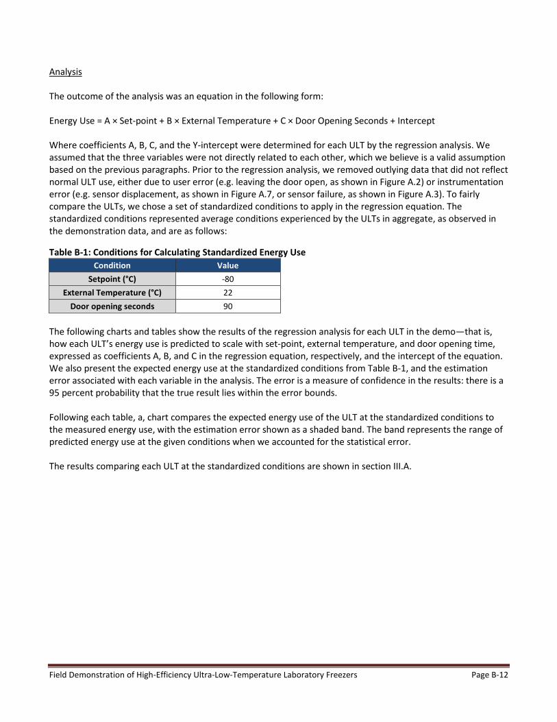
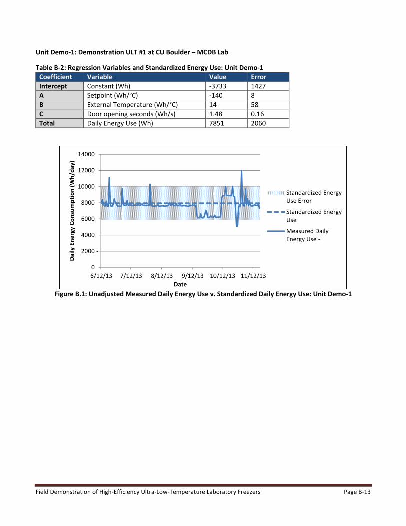
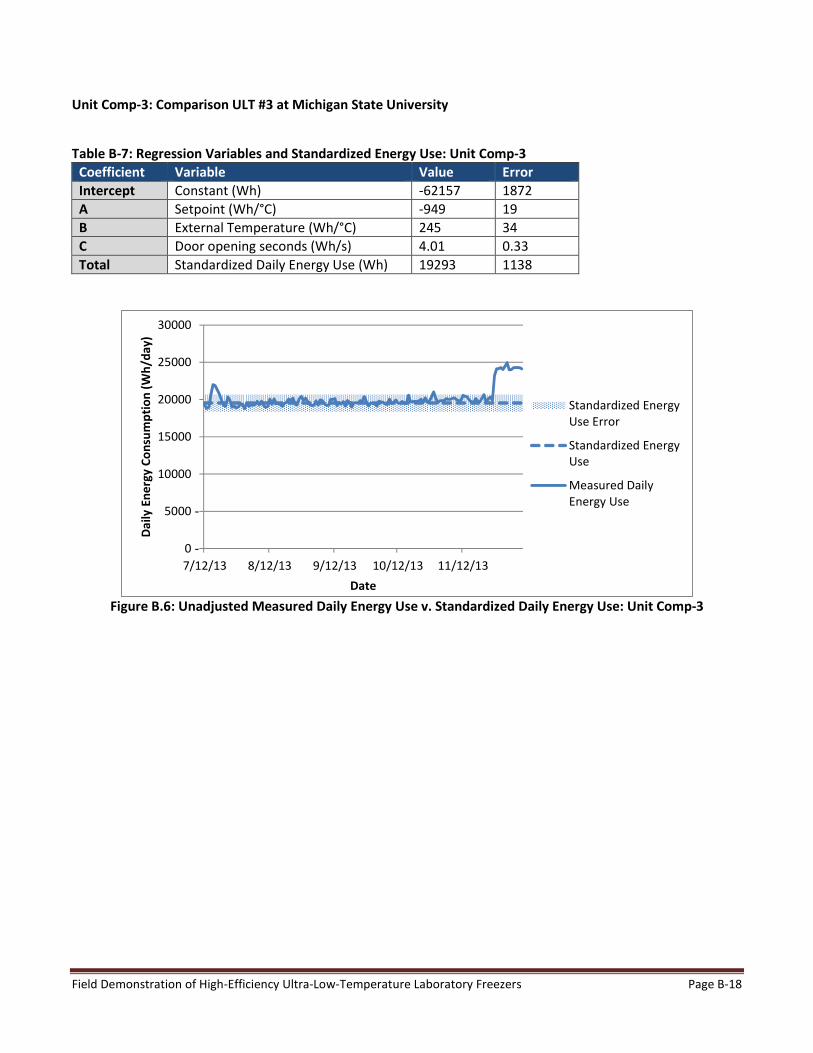
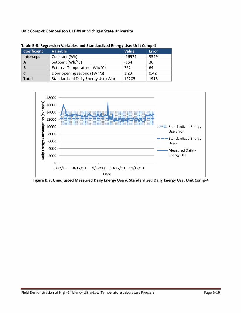
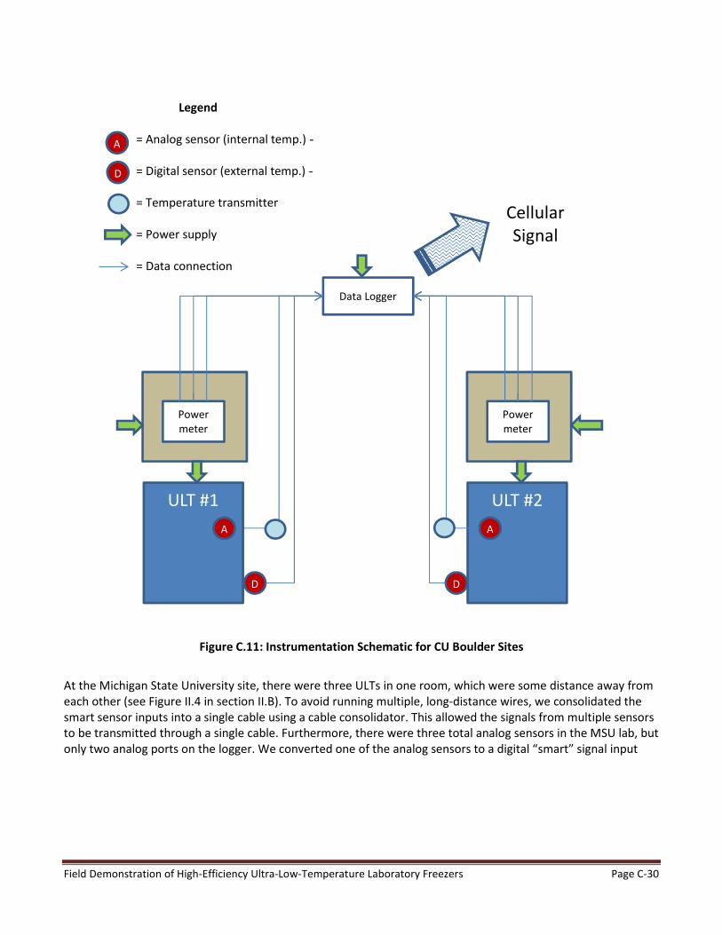
Legend
A
D
= Analog sensor (internal temp)shy
= Digital sensor (external temp)shy
Data Logger
Cellular
Signal
ULT 1
D
A
Power
meter
ULT 2
D
A
Power
meter
= Temperature transmitter
= Power supply
= Data connection
Figure C11 Instrumentation Schematic for CU Boulder Sites
At the Michigan State University site there were three ULTs in one room which were some distance away from
each other (see Figure II4 in section IIB) To avoid running multiple long-distance wires we consolidated the
smart sensor inputs into a single cable using a cable consolidator This allowed the signals from multiple sensors
to be transmitted through a single cable Furthermore there were three total analog sensors in the MSU lab but
only two analog ports on the logger We converted one of the analog sensors to a digital ldquosmartrdquo signal input
Field Demonstration of High-Efficiency Ultra-Low-Temperature Laboratory Freezers Page C-30
meter
using an Onset S-CIA-CM14 12-bit 4-20 mA input adapter34 We included a separate 12 VDC power supply to
supply power to that analog sensor Figure C12 shows a diagram of the instrumentation setup at the Michigan
State University site
Legend
A
D
= Analog sensor (internal temp)shy
= Digital sensor (external temp)shy
= Temperature transmitter Wi-fi Signal
Data
Logger
ULT 1 ULT 2 ULT 3
D
A A
D
A
D
Power
meter
Consolidator
box
Power
Consolidator
box
Power
meter
Input adapter
= Power supply
= Data connection
Figure C12 Instrumentation Schematic for Michigan State University Lab
34 Onset Computer Corporation 12-Bit 4-20 mA Input Adapter Manual
Field Demonstration of High-Efficiency Ultra-Low-Temperature Laboratory Freezers Page C-31
Door Openings
We monitored door openings using a stand-alone state logger35 The state logger consisted of a logging device
on the main body of the ULT with a magnetic switch and a magnet attached to the outer door Each time a user
opened the door the magnetic connection would be broken and the logger would record the timestamp Once
the door was closed the logger would sense the magnetic field and record another timestamp Figure C13
shows a schematic diagram of the data logger and magnet while Figure C14 shows a photograph of the logger
attached to a door We calculated the duration of each door opening by subtracting each door-open timestamp
from its subsequent door-closed timestamp
Internal Magnetic Switch
Magnet
Picture credit Onset Computer Corporation
Figure C13 Diagram of Logger and Magnet
35 Onset Computer Corporation HOBO State Data Logger (UX90-001x) Manual
Field Demonstration of High-Efficiency Ultra-Low-Temperature Laboratory Freezers Page C-32
Photo credit Dave Trumpie
Figure C14 Photograph of Logger and Magnet on ULT
This measurement approach is ideal for intermittent events because it does not require much logging memory
(as opposed to for example recording the openclosed state every second) On the other hand the door sensor
was not compatible with the one-minute intervals being recorded by the energy and temperature logger and so
we could not upload data remotely Instead someone visited each site on a periodic basis to collect the door
data from the logger The periodic data retrieval was a precaution to guard against data loss each of the door
loggers had enough memory to collect the door data for the entire measurement period even with a far larger
rate of door openings than was observed
Field Demonstration of High-Efficiency Ultra-Low-Temperature Laboratory Freezers Page C-33
Appendix D Calculating Power Factor
Power factor is ldquothe ratio of real power being used in a circuit expressed in watts to the apparent power drawn
from the power line expressed in volt-amperesrdquo36 The real and reactive power values are expressed as vectors
at right angles to each other on an electrical phase diagram while their vector sum is the total (apparent)
power This effect is illustrated in Figure D1
Total power
(VA)
Real power (W)shy
Reactive power
(VAR)
Figure D1 Relationship Among Power Variables
Power factor can be calculated from the measured energy data using the Pythagorean theorem
(Real power)2 + (Reactive power)2 = (Total power)2
Real power Power factor =
Total powershy
Real powershyPower factor =
(Real power)2 + (Reactive power)2
ldquoPowerrdquo can be replaced with ldquoenergyrdquo in the equation in order to use the measured data because the ldquohoursrdquo
variable in the energy values cancels out
Real energy Power factor =
(Real energy)2 + (Reactive energy)2
Figure D2 compares electrical phase diagrams for equipment with a high power factor and low power factor on
the left and right respectively
36 Capehart B Turner W and Kennedy W Guide to Energy Management 7th Edition The Fairmont Press 2012
Field Demonstration of High-Efficiency Ultra-Low-Temperature Laboratory Freezers Page D-34
Real power (W)
Reactive
power
(VAR)
Total power
(VA)
Real power (W)
Reactive
power
(VAR)
Total power
(VA)
Equipment with a high power factor (good)
Real power asymp Total power
Equipment with a low power factor (bad)
Real power ltlt Total power
Figure D2 Comparison of Power Factor for Different Equipment
Field Demonstration of High-Efficiency Ultra-Low-Temperature Laboratory Freezers Page D-35shy

meter
using an Onset S-CIA-CM14 12-bit 4-20 mA input adapter34 We included a separate 12 VDC power supply to
supply power to that analog sensor Figure C12 shows a diagram of the instrumentation setup at the Michigan
State University site
Legend
A
D
= Analog sensor (internal temp)shy
= Digital sensor (external temp)shy
= Temperature transmitter Wi-fi Signal
Data
Logger
ULT 1 ULT 2 ULT 3
D
A A
D
A
D
Power
meter
Consolidator
box
Power
Consolidator
box
Power
meter
Input adapter
= Power supply
= Data connection
Figure C12 Instrumentation Schematic for Michigan State University Lab
34 Onset Computer Corporation 12-Bit 4-20 mA Input Adapter Manual
Field Demonstration of High-Efficiency Ultra-Low-Temperature Laboratory Freezers Page C-31
Door Openings
We monitored door openings using a stand-alone state logger35 The state logger consisted of a logging device
on the main body of the ULT with a magnetic switch and a magnet attached to the outer door Each time a user
opened the door the magnetic connection would be broken and the logger would record the timestamp Once
the door was closed the logger would sense the magnetic field and record another timestamp Figure C13
shows a schematic diagram of the data logger and magnet while Figure C14 shows a photograph of the logger
attached to a door We calculated the duration of each door opening by subtracting each door-open timestamp
from its subsequent door-closed timestamp
Internal Magnetic Switch
Magnet
Picture credit Onset Computer Corporation
Figure C13 Diagram of Logger and Magnet
35 Onset Computer Corporation HOBO State Data Logger (UX90-001x) Manual
Field Demonstration of High-Efficiency Ultra-Low-Temperature Laboratory Freezers Page C-32
Photo credit Dave Trumpie
Figure C14 Photograph of Logger and Magnet on ULT
This measurement approach is ideal for intermittent events because it does not require much logging memory
(as opposed to for example recording the openclosed state every second) On the other hand the door sensor
was not compatible with the one-minute intervals being recorded by the energy and temperature logger and so
we could not upload data remotely Instead someone visited each site on a periodic basis to collect the door
data from the logger The periodic data retrieval was a precaution to guard against data loss each of the door
loggers had enough memory to collect the door data for the entire measurement period even with a far larger
rate of door openings than was observed
Field Demonstration of High-Efficiency Ultra-Low-Temperature Laboratory Freezers Page C-33
Appendix D Calculating Power Factor
Power factor is ldquothe ratio of real power being used in a circuit expressed in watts to the apparent power drawn
from the power line expressed in volt-amperesrdquo36 The real and reactive power values are expressed as vectors
at right angles to each other on an electrical phase diagram while their vector sum is the total (apparent)
power This effect is illustrated in Figure D1
Total power
(VA)
Real power (W)shy
Reactive power
(VAR)
Figure D1 Relationship Among Power Variables
Power factor can be calculated from the measured energy data using the Pythagorean theorem
(Real power)2 + (Reactive power)2 = (Total power)2
Real power Power factor =
Total powershy
Real powershyPower factor =
(Real power)2 + (Reactive power)2
ldquoPowerrdquo can be replaced with ldquoenergyrdquo in the equation in order to use the measured data because the ldquohoursrdquo
variable in the energy values cancels out
Real energy Power factor =
(Real energy)2 + (Reactive energy)2
Figure D2 compares electrical phase diagrams for equipment with a high power factor and low power factor on
the left and right respectively
36 Capehart B Turner W and Kennedy W Guide to Energy Management 7th Edition The Fairmont Press 2012
Field Demonstration of High-Efficiency Ultra-Low-Temperature Laboratory Freezers Page D-34
Real power (W)
Reactive
power
(VAR)
Total power
(VA)
Real power (W)
Reactive
power
(VAR)
Total power
(VA)
Equipment with a high power factor (good)
Real power asymp Total power
Equipment with a low power factor (bad)
Real power ltlt Total power
Figure D2 Comparison of Power Factor for Different Equipment
Field Demonstration of High-Efficiency Ultra-Low-Temperature Laboratory Freezers Page D-35shy

Real power (W)
Reactive
power
(VAR)
Total power
(VA)
Real power (W)
Reactive
power
(VAR)
Total power
(VA)
Equipment with a high power factor (good)
Real power asymp Total power
Equipment with a low power factor (bad)
Real power ltlt Total power
Figure D2 Comparison of Power Factor for Different Equipment
Field Demonstration of High-Efficiency Ultra-Low-Temperature Laboratory Freezers Page D-35shy