fiber optics iv - testing - pdhonline.com · training series (neets) section on fiber optic cable...
TRANSCRIPT
PDHonline Course E311 (3 PDH)
Fiber Optics IV - Testing
2012
Instructor: Lee Layton, PE
PDH Online | PDH Center5272 Meadow Estates Drive
Fairfax, VA 22030-6658Phone & Fax: 703-988-0088
www.PDHonline.orgwww.PDHcenter.com
An Approved Continuing Education Provider
www.PDHcenter.com PDH Course E311 www.PDHonline.org
© Lee Layton. Page 2 of 38
www.PDHcenter.com
Fiber Optic Systems IV - Testing
Lee Layton, P.E
Table of Contents
Section Page
Preface ……………………………….….. 3
Introduction ………………………….….. 4
Fiber Optic Measurement Techniques ….. 5
Summary ……………………………….. 36
This series of courses are based on the Navy Electricity and Electronics
Training Series (NEETS) section on Fiber Optic cable systems. The NEETS
material has been reformatted for readability and ease of use as a continuing
education course. The NEETS series is produced by the Naval Education and
Training Professional Development and Technology Center.

www.PDHcenter.com PDH Course E311 www.PDHonline.org
© Lee Layton. Page 3 of 38
Preface
This is the forth in a series of five courses about fiber optic cable systems. The series covers
fiber optics from basic light theory transmission to cables, connectors, testing, and signal
transmission.
The complete series includes these five courses:
1. Fiber Optics I – Theory
2. Fiber Optics II – Cable Design
3. Fiber Optics III – Connectors
4. Fiber Optics IV – Testing
5. Fiber Optics V – Equipment
The first course, Fiber Optics I –Theory, is an overview of the technology of fiber optic cables
including a description of the components, history, and advantages of fiber optic cables. This
course also discusses the electromagnetic theory of light and describes the properties of light
reflection, refraction, diffusion, and absorption.
The second course, Fiber Optics II – Cable Design, explains the basic construction of fiber optic
cables including the types of cables, cable properties, and performance characteristics. The
course reviews multimode, single mode step-index and graded index fibers, and fabrication
procedures.
The third course, Fiber Optics III - Connectors, describes fiber optic splices, connectors,
couplers and the types of connections they form in systems. It includes a discussion on the types
of extrinsic and intrinsic coupling losses, fiber alignment and fiber mismatch problems, and fiber
optic mechanical and fusion splices.
The fourth course, Fiber Optics IV - Testing, describes the optical fiber and optical connection
laboratory measurements used to evaluate fiber optic components and system performance,
including the near-field and far-field optical power distribution of an optical fiber. This course
also reviews optical time-domain reflectometry (OTDR).
The fifth course, Fiber Optics V - Equipment, explains the principal properties of an optical
source and fiber optic transmitters, the optical emission properties of semiconductor light-
emitting diodes (LEDs) and laser diodes (LDs), and explains the operational differences between
surface-emitting LEDs (SLEDs), edge-emitting LEDs (ELEDs), superluminescent diodes
(SLDs), and laser diodes.
It is not necessary to take the courses in sequence. However, for best comprehension it is
suggested that the courses be taken in the order presented.

www.PDHcenter.com PDH Course E311 www.PDHonline.org
© Lee Layton. Page 4 of 38
Introduction
This is Volume IV of five volumes on fiber optics systems. This volume is concerned with the
measurement and testing procedures used with of fiber optic cables.
This course describes the optical fiber and optical connection laboratory measurements used to
evaluate fiber optic components and system performance, including the near-field and far-field
optical power distribution of an optical fiber. Optical fiber launch conditions and modal effects
that affect optical fiber and optical connection measurements are reviewed. The course also
reviews optical time-domain reflectometry (OTDR) and how to interpret an optical time-domain
reflectometer (OTDR) trace.
www.PDHcenter.com PDH Course E311 www.PDHonline.org
© Lee Layton. Page 5 of 38
Fiber Optic Measurement Techniques
Fiber optic data links operate reliably if fiber optic component manufacturers and end users
perform the necessary laboratory and field measurements. Manufacturers must test how
component designs, material properties, and fabrication techniques affect the performance of
fiber optic components. These tests can be categorized as design tests or quality control tests.
Design tests are conducted during the development of a component. Design tests characterize the
component's performance (optical, mechanical, and environmental) in the intended application.
Once the component performance is characterized, the manufacturer generally only conducts
quality control tests. Quality control tests verify that the parts produced are the same as the parts
the design tests were conducted on. When manufacturers ship fiber optic components, they
provide quality control data detailing the results of measurements performed during or after
component fabrication.
End users (equipment manufacturers, maintenance personnel, test personnel, and so on) should
measure some of these parameters upon receipt before installing the component into the fiber
optic data link. These tests determine if the component has been damaged in the shipping
process. In addition, end users should measure some component parameters after installing or
repairing fiber optic components in the field. The values obtained can be compared to the system
installation specifications. These measurements determine if the installation or repair process has
degraded component performance and will affect data link operation.
Whenever a measurement is made, it should be made using a standard measurement procedure.
For most fiber optic measurements, these standard procedures are documented by the Electronics
Industries Association/Telecommunications Industries Association (EIA/TIA). Each component
measurement procedure is assigned a unique number given by EIA/TIA-455-X. The X is a
sequential number assigned to that particular component test procedure. System level test
procedures are assigned unique numbers given by EIA/TIA-526-X.
Laboratory Measurements
Providing a complete description of every laboratory measurement performed by manufacturers
and end users is impossible. This section only provides descriptions of optical fiber and optical
connection measurements that are important to system operation. The list of optical fiber and
optical connection laboratory measurements described in this section includes the following:
Attenuation
Cutoff wavelength (single mode)
Bandwidth (multimode)
Chromatic dispersion
Fiber geometry
Core diameter
Numerical aperture (multimode)
Mode field diameter (single mode)
Insertion loss

www.PDHcenter.com PDH Course E311 www.PDHonline.org
© Lee Layton. Page 6 of 38
Return loss and reflectance
End users routinely perform optical fiber measurements to measure fiber power loss and fiber
information capacity. End users may also perform optical fiber measurements to measure fiber
geometrical properties. Optical fiber power loss measurements include attenuation and cutoff
wavelength. Optical fiber information capacity measurements include chromatic dispersion and
bandwidth. Fiber geometrical measurements include cladding diameter, core diameter, numerical
aperture, and mode field diameter. Optical connection measurements performed by end users in
the laboratory include insertion loss and reflectance or return loss.
Attenuation
Attenuation is the loss of optical power as light travels along the fiber. It is a result of absorption,
scattering, bending, and other loss mechanisms. Each loss mechanism contributes to the total
amount of fiber attenuation.
End users measure the total attenuation of a fiber at the operating wavelength (). The total
attenuation (A) between an arbitrary point X and point Y located on the fiber is,
A = 10 *
Where,
A = Total attenuation, dB.
Px = The power output at point X.
Py = The power output at point Y
Point X is assumed to be closer to the optical source than point Y. The total amount of
attenuation will vary with changes in wavelength .
The attenuation coefficient () or attenuation rate, is,
=
Where,
= Attenuation coefficient (), dB/km.
A = Total attenuation, db
L = Distance between points X and Y, km.
Alpha () is a positive number because Px is always larger than Py. The attenuation coefficient
will also vary with changes in lambda (.
Cutback Method

www.PDHcenter.com PDH Course E311 www.PDHonline.org
© Lee Layton. Page 7 of 38
In laboratory situations, end users perform the cutback method for measuring the total
attenuation of an optical fiber. The cutback method involves comparing the optical power
transmitted through a long piece of test fiber to the power present at the beginning of the fiber.
The cutback method for measuring multimode fiber attenuation is EIA/TIA-455-46. The cutback
method for measuring single mode fiber attenuation is EIA/TIA-455-78. The basic measurement
process is the same for both of these procedures. The test method requires that the test fiber of
known length (L) be cut back to an approximate 2-m length. This cut back causes the destruction
of 2-m of fiber. This method requires access to both fiber ends. Each fiber end should be
properly prepared to make measurements. EIA/TIA-455-57 describes how to properly prepare
fiber ends for measurement purposes.
Figure 1 illustrates the cutback method for measuring fiber attenuation. The cutback method
begins by measuring, with an optical power meter, the output power P1 of the test fiber of known
length (L) as shown in the top view of Figure 1. Without disturbing the input light conditions,
the test fiber is cut back to an approximate 2-m length. The output power P2 of the shortened test
fiber is then measured as shown in the bottom view of Figure 1. The fiber attenuation AT and the
attenuation coefficient alpha () are then calculated.
Figure 1. - Cutback method for measuring fiber attenuation
Launch Conditions
www.PDHcenter.com PDH Course E311 www.PDHonline.org
© Lee Layton. Page 8 of 38
Measurement personnel must pay attention to how optical power is launched into the fiber when
measuring fiber attenuation. Different distributions of launch power (launch conditions) can
result in different attenuation measurements. This is more of a problem with multimode fiber
than single mode fiber. For single mode fiber, optical power must be launched only into the
fundamental mode. This is accomplished using a mode filter on the fiber. For multimode fiber,
the distribution of power among the modes of the fiber must be controlled. This is accomplished
by controlling the launch spot size and angular distribution.
The launch spot size is the area of the fiber face illuminated by the light beam from the optical
source. The diameter of the spot depends on the size of the optical source and the properties of
the optical elements (lenses, and so on) between the source and the fiber end face. The angular
distribution is the angular extent of the light beam from the optical source incident on the fiber
end face. The launch angular distribution also depends on the size of the optical source and the
properties of the optical elements between the optical source and the fiber end face.
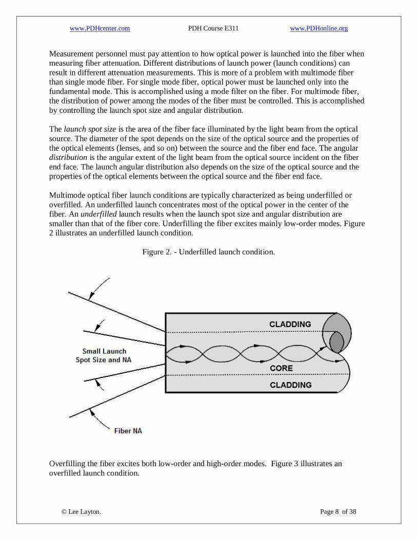
Multimode optical fiber launch conditions are typically characterized as being underfilled or
overfilled. An underfilled launch concentrates most of the optical power in the center of the
fiber. An underfilled launch results when the launch spot size and angular distribution are
smaller than that of the fiber core. Underfilling the fiber excites mainly low-order modes. Figure
2 illustrates an underfilled launch condition.
Figure 2. - Underfilled launch condition.
Overfilling the fiber excites both low-order and high-order modes. Figure 3 illustrates an
overfilled launch condition.

www.PDHcenter.com PDH Course E311 www.PDHonline.org
© Lee Layton. Page 9 of 38
An overfilled launch condition occurs when the launch spot size and angular distribution are
larger than that of the fiber core. Incident light that falls outside the fiber core is lost. In addition,
light that is incident at angles greater than the angle of acceptance of the fiber core is lost.
Figure 3. - Overfilled launch condition.
In attenuation measurements, cladding-mode strippers and mode filters eliminate the effects that
high-order modes have on attenuation results. A cladding-mode stripper is a device that removes
any cladding mode power from the fiber. Most cladding-mode strippers consist of a material
with a refractive index greater than that of the fiber cladding. For most fibers, the fiber coating
acts as an excellent cladding-mode stripper.
A mode filter is a device that attenuates specific modes propagating in the core of an optical
fiber. Mode filters generally involve wrapping the test fiber around a mandrel. For multimode,
tight bends tend to remove high-order modes from the fiber. This type of mode filter is known as
a mandrel wrap mode filter. For multimode fibers, mode filters remove high-order propagating
modes and are individually tailored and adjusted for a specific fiber type.
For single mode fibers, a mode filter is used to eliminate the second-order mode from
propagating along the fiber. The propagation of the second-order mode will affect attenuation
measurements. Fiber attenuation caused by the second-order mode depends on the operating
wavelength, the fiber bend radius and length.
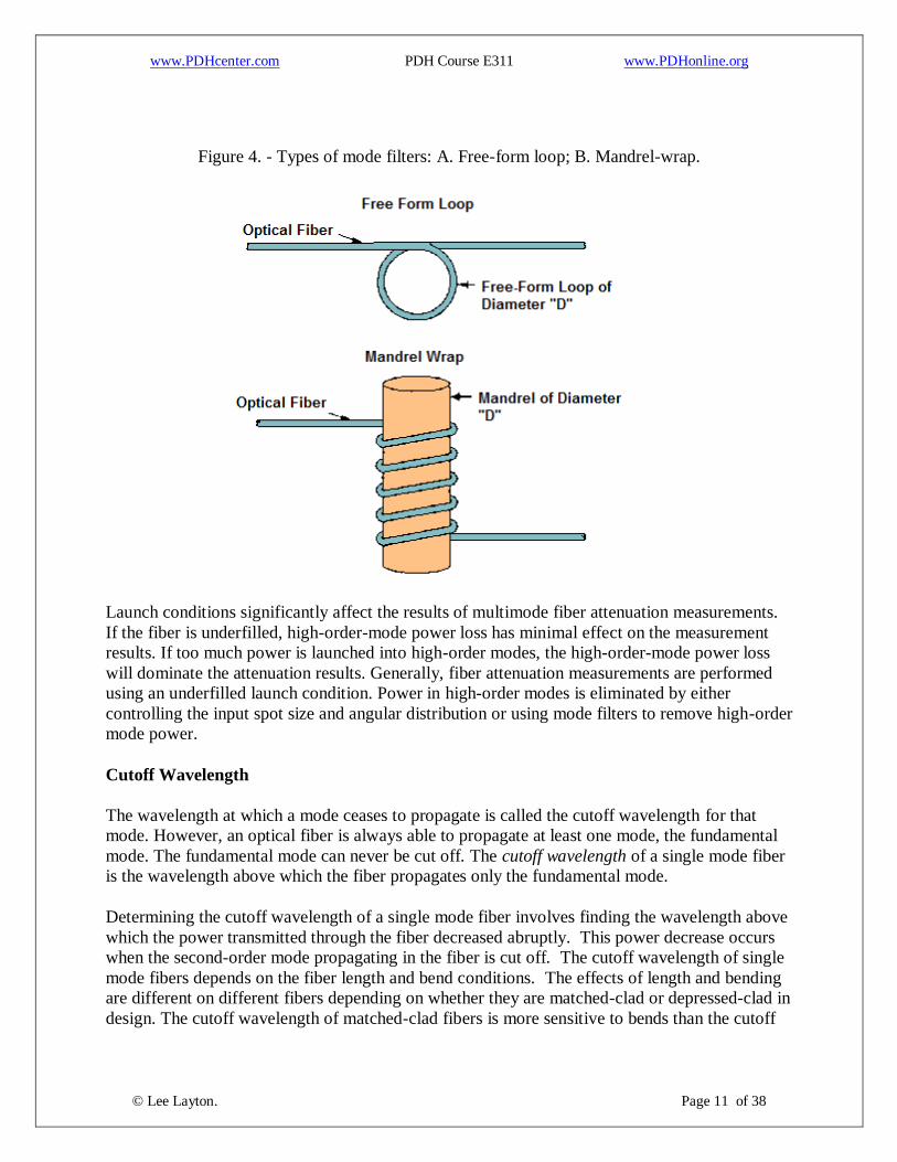
The two most common types of mode filters are free-form loops and mandrel wraps. Figure 4
illustrates the free-form loop and mandrel-wrap types of mode filters. Mandrel wraps for
multimode fibers consist of several wraps (approximately 4 or 5) around a mandrel. A 20-mm
diameter mandrel is typically used for 62.5 m fiber. Mandrel wraps for single mode fibers

www.PDHcenter.com PDH Course E311 www.PDHonline.org
© Lee Layton. Page 10 of 38
consist of a single wrap around a 30-mm diameter mandrel. Another common mode filter for
single mode fibers is a 30-mm diameter circular free-form loop.
www.PDHcenter.com PDH Course E311 www.PDHonline.org
© Lee Layton. Page 11 of 38
Figure 4. - Types of mode filters: A. Free-form loop; B. Mandrel-wrap.
Launch conditions significantly affect the results of multimode fiber attenuation measurements.
If the fiber is underfilled, high-order-mode power loss has minimal effect on the measurement
results. If too much power is launched into high-order modes, the high-order-mode power loss
will dominate the attenuation results. Generally, fiber attenuation measurements are performed
using an underfilled launch condition. Power in high-order modes is eliminated by either
controlling the input spot size and angular distribution or using mode filters to remove high-order
mode power.
Cutoff Wavelength
The wavelength at which a mode ceases to propagate is called the cutoff wavelength for that
mode. However, an optical fiber is always able to propagate at least one mode, the fundamental
mode. The fundamental mode can never be cut off. The cutoff wavelength of a single mode fiber
is the wavelength above which the fiber propagates only the fundamental mode.
Determining the cutoff wavelength of a single mode fiber involves finding the wavelength above
which the power transmitted through the fiber decreased abruptly. This power decrease occurs
when the second-order mode propagating in the fiber is cut off. The cutoff wavelength of single
mode fibers depends on the fiber length and bend conditions. The effects of length and bending
are different on different fibers depending on whether they are matched-clad or depressed-clad in
design. The cutoff wavelength of matched-clad fibers is more sensitive to bends than the cutoff

www.PDHcenter.com PDH Course E311 www.PDHonline.org
© Lee Layton. Page 12 of 38
wavelength of depressed-clad fibers. The cutoff wavelength of depressed-clad fibers is more
sensitive to length than the cutoff wavelength of matched-clad fibers.
Cutoff wavelength may be measured on uncabled or cabled single mode fibers. A slightly
different procedure is used in each case, but the basic measurement process is the same. The test
method for uncabled single mode fiber cutoff wavelength is EIA/TIA-455-80. The test method
for cabled single mode fiber cutoff wavelength is EIA/TIA-455-170. The fiber cutoff wavelength
(cf) measured under EIA/TIA-455-80 will generally be higher than the cable cutoff wavelength
(cc) measured under EIA/TIA-455-170. The difference is due to the fiber bends introduced
during the cable manufacturing process.
Each test method describes the test equipment (input optics, mode filters, and cladding-mode
strippers) necessary for the test. Cutoff wavelength measurements require an overfilled launch
over the full range of test wavelengths. Since the procedures for measuring the cutoff wavelength
of uncabled and cabled single mode fibers are essentially the same, only the test method for
measuring the cutoff wavelength of uncabled fiber is discussed.
Measuring the cutoff wavelength involves comparing the transmitted power from the test fiber
with that of a reference fiber at different wavelengths. The reference fiber can be the same piece
of single mode fiber with small bends introduced or a piece of multimode fiber. If the same fiber
with small bends is used as the reference fiber, the technique is called the bend-reference
technique. If a piece of multimode fiber is used as the reference fiber, the technique is called the
multimode-reference technique.
For both techniques, the test fiber is loosely supported in a single-turn with a constant radius of
140 mm. Figure 5 shows this single-turn configuration. The transmitted signal power Ps () is
then recorded while scanning the wavelength range in increments of 10 nm or less. The launch
and detection conditions are not changed while scanning over the range of wavelengths. The
wavelength range scanned encompasses the expected cutoff wavelength.
Figure 5. - Single-turn configuration for the test fiber.
The reference power measurement is then made. For the bend-reference technique, the launch
and detection conditions are not changed, but an additional bend is added to the test fiber. The
test fiber is bent to a radius of 30 mm or less to suppress the second-order mode at all the
scanned wavelengths. For the multimode-reference technique, the single mode fiber is replaced
with a 2-m length of multimode fiber. The transmitted signal power Pr() is recorded while

www.PDHcenter.com PDH Course E311 www.PDHonline.org
© Lee Layton. Page 13 of 38
scanning the same wavelength range in the same increments of 10 nm or less. The attenuation
A() at each wavelength is calculated as follows,
A() = 10 *
Where,
A() = Attenuation at each wavelength.
Ps() = Transmitted signal power for the sample fiber.
Pr) = Transmitted signal power for the reference fiber.
Figure 6 shows a sample attenuation plot generated using the bend-reference technique. The
longest wavelength at which A) is equal to 0.1 db is the fiber cutoff wavelength (cf). cf is
marked on Figure 6.
Figure 6. - Fiber cutoff wavelength determined by the bend-reference technique.
www.PDHcenter.com PDH Course E311 www.PDHonline.org
© Lee Layton. Page 14 of 38
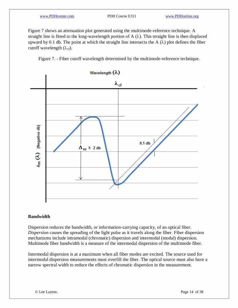
Figure 7 shows an attenuation plot generated using the multimode-reference technique. A
straight line is fitted to the long-wavelength portion of A (). This straight line is then displaced
upward by 0.1 db. The point at which the straight line intersects the A () plot defines the fiber
cutoff wavelength (cf).
Figure 7. - Fiber cutoff wavelength determined by the multimode-reference technique.
Bandwidth
Dispersion reduces the bandwidth, or information-carrying capacity, of an optical fiber.
Dispersion causes the spreading of the light pulse as it travels along the fiber. Fiber dispersion
mechanisms include intramodal (chromatic) dispersion and intermodal (modal) dispersion.
Multimode fiber bandwidth is a measure of the intermodal dispersion of the multimode fiber.
Intermodal dispersion is at a maximum when all fiber modes are excited. The source used for
intermodal dispersion measurements must overfill the fiber. The optical source must also have a
narrow spectral width to reduce the effects of chromatic dispersion in the measurement.

www.PDHcenter.com PDH Course E311 www.PDHonline.org
© Lee Layton. Page 15 of 38
There are two basic techniques for measuring the modal bandwidth of an optical fiber. The first
technique characterizes dispersion by measuring the impulse response h(t) of the fiber in the time
domain. The second technique characterizes modal dispersion by measuring the baseband
Frequency response H(f) of the fiber in the frequency domain. H(f) is the power transfer function
of the fiber at the baseband frequency (f). H(f) is also the Fourier transform of the power impulse
response h(t). Only the Frequency response method is described here.
The test method for measuring the bandwidth of multimode fibers in the frequency domain is
EIA/TIA-455-30. Signals of varying frequencies (f) are launched into the test fiber and the power
exiting the fiber at the launched fundamental frequency measured. This optical output power is
denoted as Pout( f). The test fiber is then cut back or replaced with a short length of fiber of the
same type. Signals of the same frequency are launched into the cut-back fiber and the power
exiting the cut-back fiber at the launched fundamental frequency measured. The optical power
exiting the cutback or replacement fiber is denoted as Pin(f). The magnitude of the optical fiber
Frequency response is,
H(f) =
Where,
H(f) = Frequency response at the baseband frequency.
Pin(f) = Power exiting the cutback fiber at the fundamental frequency.
Pout( f) = Power exiting the fiber at the fundamental frequency.
The fiber bandwidth is defined as the lowest frequency at which the magnitude of the fiber
Frequency response has decreased to one-half its zero-frequency value. This is the -3 decibel
(db) optical power frequency (f3db). This frequency is referred to as the fiber bandwidth.
Bandwidth is normally given in units of megahertz-kilometers (MHz-km). Converting the -3 db
fiber bandwidth to a unit length assists in the analysis and comparison of optical fiber
performance. For long lengths of fiber (>1km), the method for normalization is to multiply the
length times the measured bandwidth.
Chromatic Dispersion
Chromatic, or intramodal, dispersion occurs in both single mode and multimode optical fibers.
Chromatic dispersion occurs because different colors of light travel through the fiber at different
speeds. Since the different colors of light have different velocities, some colors arrive at the fiber
end before others. This delay difference is called the differential group delay () per unit length.
This differential group delay leads to pulse broadening.
Chromatic dispersion is measured using EIA/TIA-455-168 in the time domain. Chromatic
dispersion is also measured in the frequency domain using EIA/TIA-455-169 and EIA/TIA-455-
175. These methods measure the composite optical fiber material and waveguide dispersion. In
www.PDHcenter.com PDH Course E311 www.PDHonline.org
© Lee Layton. Page 16 of 38
this course, we limit the discussion on chromatic dispersion to the time domain method described
in EIA/TIA-455-168.
The chromatic dispersion of multimode graded-index and single mode fiber is obtained by
measuring fiber group delays in the time domain. These measurements are made using multi-
wavelength sources or multiple sources of different wavelengths. A multi-wavelength source
could be a wavelength-selectable laser.
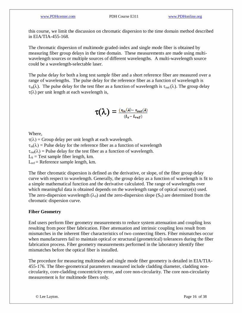
The pulse delay for both a long test sample fiber and a short reference fiber are measured over a
range of wavelengths. The pulse delay for the reference fiber as a function of wavelength is
in(). The pulse delay for the test fiber as a function of wavelength is out (). The group delay
() per unit length at each wavelength is,
=
Where,
= Group delay per unit length at each wavelength.
in = Pulse delay for the reference fiber as a function of wavelength
out = Pulse delay for the test fiber as a function of wavelength.
LS = Test sample fiber length, km.
Lref = Reference sample length, km.
The fiber chromatic dispersion is defined as the derivative, or slope, of the fiber group delay
curve with respect to wavelength. Generally, the group delay as a function of wavelength is fit to
a simple mathematical function and the derivative calculated. The range of wavelengths over
which meaningful data is obtained depends on the wavelength range of optical source(s) used.
The zero-dispersion wavelength (0) and the zero-dispersion slope (S0) are determined from the
chromatic dispersion curve.
Fiber Geometry
End users perform fiber geometry measurements to reduce system attenuation and coupling loss
resulting from poor fiber fabrication. Fiber attenuation and intrinsic coupling loss result from
mismatches in the inherent fiber characteristics of two connecting fibers. Fiber mismatches occur
when manufacturers fail to maintain optical or structural (geometrical) tolerances during the fiber
fabrication process. Fiber geometry measurements performed in the laboratory identify fiber
mismatches before the optical fiber is installed.
The procedure for measuring multimode and single mode fiber geometry is detailed in EIA/TIA-
455-176. The fiber-geometrical parameters measured include cladding diameter, cladding non-
circularity, core-cladding concentricity error, and core non-circularity. The core non-circularity
measurement is for multimode fibers only.

www.PDHcenter.com PDH Course E311 www.PDHonline.org
© Lee Layton. Page 17 of 38
Other test methods are available for measuring other multimode and single mode fiber core
parameters. Additional test methods exist for measuring multimode fiber core diameter and NA.
For single mode fibers, the mode field diameter measurement replaces core diameter and NA
measurements. Core diameter, numerical aperture, and mode field diameter measurements are
identified and explained later.
To make fiber geometry measurements, the input end of the fiber is overfilled and any cladding
power stripped out. The output end of the fiber is prepared and viewed with a video camera.
Generally the fiber is less than 10 m in length. An objective lens magnifies the output image
(typically 20X) going to a video camera. The image from the video camera is displayed on a
video monitor and is also sent to the computer for digital analysis.
The computer analyzes the image to identify the edges of the core and cladding. The centers rc
and rg of the core and cladding, respectively, are found. The cladding diameter is defined as the
average diameter of the cladding. The cladding diameter is twice the average radius (Rg). The
core diameter is defined as the average diameter of the core. The core diameter is twice the
average core radius (Rc).
Cladding non-circularity, or ellipticity, is the difference between the smallest radius of the fiber
(Rgmin) and the largest radius (Rgmax) divided by the average cladding radius (Rg). The value of
the cladding non-circularity is expressed as a percentage.
The core-cladding concentricity error for multimode fibers is the distance between the core and
cladding centers divided by the core diameter. Multimode core-cladding concentricity error is
expressed as a percentage of the core diameter. The core-cladding concentricity error for single
mode fibers is defined as the distance between the core and cladding centers.
Core non-circularity is the difference between the smallest core radius (Rcmin) and the largest
core radius (Rcmax) divided by the core radius (Rc). The value of core non-circularity is expressed
as a percentage. Core non-circularity is measured on multimode fibers only.
Core Diameter
Core diameter is measured using EIA/TIA-455-58. The core diameter is defined from the
refractive index profile n(r) or the output near-field radiation pattern. Our discussion is limited to
measuring the core diameter directly from the output near-field radiation pattern obtained using
EIA/TIA-455-43.
The near-field power distribution is defined as the emitted power per unit area (radiance) for
each position in the plane of the emitting surface. The emitting surface is the output area of a
fiber-end face. Near-field power distributions describe the emitted power per unit area in the
near-field region. The near-field region is the region close to the fiber-end face. In the near-field
region, the distance between the fiber-end face and detector is in the micrometers (m) range.
EIA/TIA-455-43 describes the procedure for measuring the near-field power distribution of
optical waveguides. Output optics, such as lenses, magnify the fiber-end face and focus the

www.PDHcenter.com PDH Course E311 www.PDHonline.org
© Lee Layton. Page 18 of 38
fiber's image on a movable detector. Figure 8 shows an example setup for measuring the near-
field power distribution. The image is scanned in a plane by the movable detector. The image
may also be scanned by using a detector array. Detector arrays of known element size and
spacing may provide a display of the power distribution on a video monitor. A record of the
near-field power is kept as a function of scan position.

www.PDHcenter.com PDH Course E311 www.PDHonline.org
© Lee Layton. Page 19 of 38
Figure 8. - The measurement of the near-field power distribution.
The core diameter (D) is derived from the normalized output near-field radiation pattern. The
normalized near-field pattern is plotted as a function of radial position on the fiber-end face.
Figure 9 shows a plot of the normalized near-field radiation pattern as a function of scan
position.

www.PDHcenter.com PDH Course E311 www.PDHonline.org
© Lee Layton. Page 20 of 38
Figure 9. - Near-field radiation pattern.
The core diameter (D) is defined as the diameter at which the intensity is 2.5 percent of the
maximum intensity (see Figure 9). The 2.5 percent points, or the 0.025 level, intersects the
normalized curve at radial positions -a and a. The core diameter is simply equal to 2a (D=2a).
Numerical Aperture
The numerical aperture (NA) is a measurement of the ability of an optical fiber to capture light.
The NA can be defined from the refractive index profile or the output far-field radiation pattern.
Our discussion is limited to measuring the NA from the output far-field radiation pattern.
The NA of a multimode fiber having a near-parabolic refractive index profile is measured using
EIA/TIA-455-177. In EIA/TIA-455-177, the fiber NA is measured from the output far-field
radiation pattern. The far-field power distribution describes the emitted power per unit area in the
far-field region. The far-field region is the region far from the fiber-end face. The far-field power
distribution describes the emitted power per unit area as a function of angle some distance
away from the fiber-end face. The distance between the fiber-end face and detector in the far-

www.PDHcenter.com PDH Course E311 www.PDHonline.org
© Lee Layton. Page 21 of 38
field region is in the centimeters (cm) range for multimode fibers and millimeters (mm) range for
single mode fibers.
EIA/TIA-455-47 describes various procedures, or methods, for measuring the far-field power
distribution of optical waveguides. These procedures involve either an angular or spacial scan.
Figure 10 illustrates an angular and spacial scan for measuring the far-field power distribution.
Figure 10 - Angular and spacial scan methods for measuring the far-field power distribution.
Figure 10 (method A) illustrates a far-field angular scan of the fiber-end face by a rotating
detector. The fiber output radiation pattern is scanned by a rotating detector in the far-field. The
detector rotates in a spherical manner. A record of the far-field power distribution is kept as a
function of angle Theta ().
Figure 10 (method B) illustrates a far-field spacial scan of the fiber-end face by a movable
(planar) detector. In a far-field spacial scan, lens L1 performs a Fourier transform of the fiber
output near-field pattern. A second lens, L2, is positioned to magnify and relay the transformed
image to the detector plane. The image is scanned in a plane by a movable detector. The scan
www.PDHcenter.com PDH Course E311 www.PDHonline.org
© Lee Layton. Page 22 of 38
position y in the Fourier transform plane is proportional to the far-field scan angle Theta (). A
record of the far-field power distribution is kept as a function of the far-field scan angle.
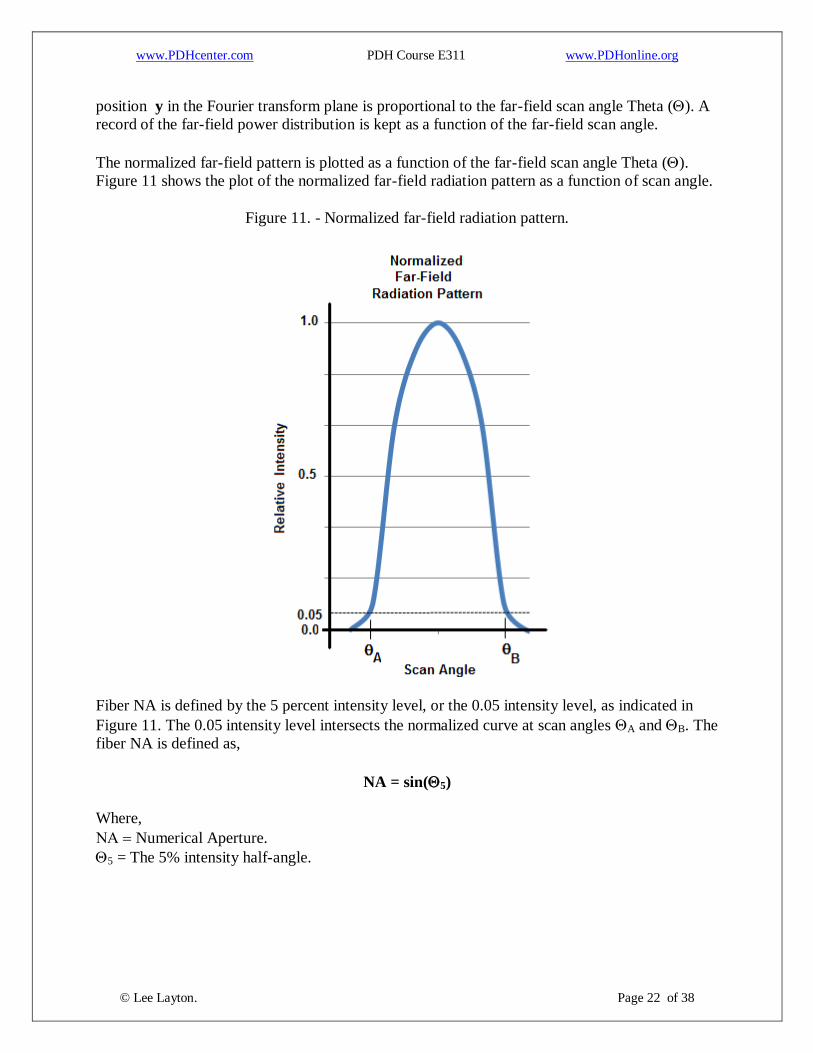
The normalized far-field pattern is plotted as a function of the far-field scan angle Theta ().
Figure 11 shows the plot of the normalized far-field radiation pattern as a function of scan angle.
Figure 11. - Normalized far-field radiation pattern.
Fiber NA is defined by the 5 percent intensity level, or the 0.05 intensity level, as indicated in
Figure 11. The 0.05 intensity level intersects the normalized curve at scan angles A and B. The
fiber NA is defined as,
NA = sin(5)
Where,
Numerical Aperture.
5 = The 5% intensity half-angle.
www.PDHcenter.com PDH Course E311 www.PDHonline.org
© Lee Layton. Page 23 of 38
The 5% intensity half-angle, 5, is determined from a and b as shown below,
5 =
Where,
5 = The 5% intensity half-angle.
a = First scan angle at the 5% intensity level, see Figure 11.
b = Second scan angle at the 5% intensity level, see Figure 11.
Mode Field Diameter
The mode field diameter (MFD) of a single mode fiber is related to the spot size of the
fundamental mode. This spot has a mode field radius w0. The mode field diameter is equal to
2w0. The size of the mode field diameter correlates to the performance of the single mode fiber.
Single mode fibers with large mode field diameters are more sensitive to fiber bending. Single
mode fibers with small mode field diameters show higher coupling losses at connections.
The mode field diameter of a single mode fiber can be measured using EIA/TIA-455-167. This
method involves measuring the output far-field power distribution of the single mode fiber using
a set of apertures of various sizes. This far-field power distribution data is transformed into the
near-field before using complex mathematical procedures. The mode field diameter is calculated
from the transformed near field data. The mathematics behind the transformation between the
far-field and near-field is too complicated for discussion here. Refer to EIA/TIA-455-167 for
information on this transformation procedure.
Insertion Loss
Insertion loss is composed of the connection coupling loss and additional fiber losses in the fiber
following the connection. In multimode fiber, fiber joints can increase fiber attenuation
following the joint by disturbing the fiber's mode power distribution (MPD). Fiber joints may
increase fiber attenuation because disturbing the MPD may excite radiative modes. Radiative
modes are unbound modes that radiate out of the fiber contributing to joint loss. In single mode
fibers, fiber joints can cause the second-order mode to propagate in the fiber following the joint.
As long as the coupling loss of the connection is small, neither radiative modes (multimode
fiber) or the second-order mode (single mode fiber) are excited.
Insertion loss of both multimode and single mode interconnection devices is measured using
EIA/TIA-455-34. For some applications an overfill launch condition is used at the input fiber.
For other applications a mandrel wrap may be used to strip out high-order mode power. The
length of fiber before the connection and after the connection may be specified for some
applications. Power measurements are made on an optical fiber or fiber optic cable before the

www.PDHcenter.com PDH Course E311 www.PDHonline.org
© Lee Layton. Page 24 of 38
joint is inserted and after the joint is made. Figure 12 illustrates the mandrel wrap method of
measuring the insertion loss of an interconnecting device in EIA/TIA-455-34.
Figure 12. - Insertion loss measurement of an interconnecting device.
Initial power measurements at the detector (P0) and at the source monitoring equipment (PM0) are
taken before inserting the interconnecting device into the test setup. The test fiber is then cut at
the location specified by the end user. The cut results in a fiber of lengths L1 and L2 before and
after the interconnection device that simulates the actual system configuration. After
interconnection, the power at the detector (P1) and at the source monitoring equipment (PM1) is
measured. The insertion loss is calculated as shown below,
Insertion Loss = 10 *
Where,
P1 = Power at the detector after interconnection.
P0 = Initial power measurements at the detector
PMO = Power at the monitoring equipment before interconnection.
PM1 = Power at the monitoring equipment after interconnection.
If the source power is constant, then the calculation of the insertion loss is similar to that of fiber
attenuation.
www.PDHcenter.com PDH Course E311 www.PDHonline.org
© Lee Layton. Page 25 of 38
Return Loss and Reflectance
Reflections occur at optical fiber connections. Optical power may be reflected back into the
source fiber when connecting two optical fibers. In laser-based systems, reflected power reaching
the optical source can reduce system performance by affecting the stability (operation) of the
source. In addition, multiple reflections occur in fiber optic data links containing more than one
connection. Multiple reflections can reduce data link performance by increasing the signal noise
present at the optical detector.
Reflectance is a measure of the portion of incident light that is reflected back into the source
fiber at the point of connection. Reflectance is given as a ratio (R) of the reflected light intensity
to the incident light intensity.
Return loss and reflectance are measured using EIA/TIA-455-107. They are measured using an
optical source connected to one input of a 2 x 2 fiber optic coupler. Light is launched into the
component under test through the fiber optic coupler. The light reflected from the component
under test is transmitted back through the fiber optic coupler to a detector connected to the other
input port. The optical power is measured at the output of the device under test (Po) and at the
input port of the coupler where the detector is located (Pr). Po is corrected to account for the loss
in power through the device under test. Pr is corrected to account for the loss in power through
the coupler and any other connection losses in the path. The reflectance is then given by the ratio
Pr/Po.
Return loss is the amount of loss of the reflected light compared with the power of the incident
beam at the interface. The optical return loss at the fiber interface is defined as,
Return Loss = - 10 * log (R)
Where,
Return Loss = Optical return loss at the fiber interface.
R = Portion of incident light that is reflected back into the source fiber at the point of connection.
Return loss is only the amount of optical power reflected and does not include power that is
transmitted, absorbed, or scattered.
Field Measurements
Field measurements differ from laboratory measurements because they measure the transmission
properties of installed fiber optic components. Laboratory measurements can only attempt to
simulate the actual operating conditions of installed components. Fiber optic component
properties measured in the laboratory can change after the installation of these components. End
users must perform field measurements to evaluate those properties most likely affected by the
installation or repair of fiber optic components or systems.
The discussion on field measurements is limited to optical fiber and optical connection
properties. Optical fiber and optical connection field measurements evaluate only the

www.PDHcenter.com PDH Course E311 www.PDHonline.org
© Lee Layton. Page 26 of 38
transmission properties affected by component or system installation or repair. Because optical
fiber geometrical properties, such as core and cladding diameter and numerical aperture, are not
expected to change, there is no need to re-measure these properties. The optical fiber properties
that are likely to change include fiber attenuation (loss) and bandwidth. Bandwidth changes in
the field tend to be beneficial, so field bandwidth measurement is generally not performed. If
field bandwidth measurements are required, they are essentially the same as laboratory
measurements so they will not be repeated. The optical connection properties that are likely to
change are connection insertion loss and reflectance and return loss.
The installation and repair of fiber optic components can affect system operation. Microbends
introduced during installation can increase fiber attenuation. Modal redistribution at fiber joints
can increase fiber attenuation in the fiber after the joint. Fiber breaks or faults can prevent or
severely disrupt system operation. Poor fiber connections can also increase insertion loss and
degrade transmitter and receiver performance by increasing reflectance and return loss. End
users should perform field measurements to verify that component performance is within
allowable limits so system performance is not adversely affected.
There are additional differences in measuring optical fiber and optical connection properties in
the field than in the laboratory. Field measurements require rugged, portable test equipment,
unlike the sophisticated test equipment used in the laboratory. Field test equipment must provide
accurate measurements in extreme environmental conditions. Since electrical power sources may
not always be available in the field, test equipment should allow battery operation. In addition,
while both fiber ends are available for conducting laboratory measurements, only one fiber end
may be readily available for field measurements. Even if both fiber ends are available for field
measurements, the fiber ends are normally located some distance apart. Therefore, field
measurements may require two people.
The main field measurement technique involves optical time-domain reflectometry. An optical
time-domain reflectometer (OTDR) is recommended for conducting field measurements on
installed optical fibers or links of 50 meters or more in length. An OTDR requires access to only
one fiber end. An OTDR measures the attenuation of installed optical fibers as a function of
length. It also identifies and evaluates optical connection losses along a cable link and locates
any fiber breaks or faults.
End users can also measure fiber attenuation and cable plant transmission loss using an optical
power meter and a stabilized light source. End users use this measurement technique when
optical time-domain reflectometry is not recommended. Measurements obtained with a stabilized
light source and power meter are more accurate than those obtained with an OTDR. Measuring
fiber attenuation and transmission loss using a power meter and light source requires access to
both ends of the fiber or link. An optical loss test set (OLTS) combines the power meter and
source functions into one physical unit.
Optical Time-Domain Reflectometry
End users use optical time-domain reflectometry to characterize optical fiber and optical
connection properties in the field. In optical time-domain reflectometry, an OTDR transmits an

www.PDHcenter.com PDH Course E311 www.PDHonline.org
© Lee Layton. Page 27 of 38
optical pulse through an installed optical fiber. The OTDR measures the fraction of light that is
reflected back due to Rayleigh scattering and Fresnel reflection. By comparing the amount of
light scattered back at different times, the OTDR can determine fiber and connection losses.
When several fibers are connected to form an installed cable plant, the OTDR can characterize
optical fiber and optical connection properties along the entire length of the cable plant. A fiber
optic cable plant consists of optical fiber cables, connectors, splices, mounting panels, jumper
cables, and other passive components. A cable plant does not include active components such as
optical transmitters or receivers.
The OTDR displays the backscattered and reflected optical signal as a function of length. The
OTDR plots half the power in decibels (db) versus half the distance. Plotting half the power in db
and half the distance corrects for round trip effects. By analyzing the OTDR plot, or trace, end
users can measure fiber attenuation and transmission loss between any two points along the cable
plant. End users can also measure insertion loss and reflectance of any optical connection. In
addition, end users use the OTDR trace to locate fiber breaks or faults.
Figure 13 shows an example OTDR trace of an installed cable plant. OTDR traces can have
several common characteristics. An OTDR trace begins with an initial input pulse. This pulse is
a result of Fresnel reflection occurring at the connection to the OTDR. Following this pulse, the
OTDR trace is a gradual down sloping curve interrupted by abrupt shifts. Periods of gradual
decline in the OTDR trace result from Rayleigh scattering as light travels along each fiber
section of the cable plant. Periods of gradual decline are interrupted by abrupt shifts called point
defects. A point defect is a temporary or permanent local deviation of the OTDR signal in the
upward or downward direction. Point defects are caused by connectors, splices, or breaks along
the fiber length. Point defects, or faults, can be reflective or non-reflective. An output pulse at the
end of the OTDR trace indicates the end of the fiber cable plant. This output pulse results from
Fresnel reflection occurring at the output fiber-end face.
Figure 13. - OTDR trace of an installed cable plant.

www.PDHcenter.com PDH Course E311 www.PDHonline.org
© Lee Layton. Page 28 of 38
Attenuation. - The fiber optic test method for measuring the attenuation of an installed optical
fiber using an OTDR is EIA/TIA-455-61. The accuracy of this test method depends on the user
entering the appropriate source wavelength, pulse duration, and fiber length (test range) into the
OTDR. In addition, the effective group index of the test fiber is required before the attenuation
coefficient and accurate distances can be recorded. The group index (N) is provided by fiber
manufacturers or is found using EIA/TIA-455-60. By entering correct test parameters, OTDR
fiber attenuation values will closely coincide with those measured by the cutback technique.
Test personnel can connect the test fiber directly to the OTDR or to a dead-zone fiber. This dead-
zone fiber is placed between the test fiber and OTDR to reduce the effect of the initial reflection
at the OTDR on the fiber measurement. The dead-zone fiber is inserted because minimizing the
reflection at a fiber joint is easier than reducing the reflection at the OTDR connection.
Figure 14 illustrates the OTDR measurement points for measuring the attenuation of the test
fiber using a dead-zone fiber. Fiber attenuation between two points along the test fiber is
measured on gradual down sloping sections on the OTDR trace. There should be no point defects
present along the portion of fiber being tested.

www.PDHcenter.com PDH Course E311 www.PDHonline.org
© Lee Layton. Page 29 of 38
Figure 14. - OTDR measurement points for measuring fiber attenuation using a dead-zone fiber.
OTDRs are equipped with either manual or automatic cursors to locate points of interest along
the trace. In Figure 14, a cursor is positioned at a distance zo on the rising edge of the reflection
at the end of the dead-zone fiber. Cursors are also positioned at distances z1 and z2. The cursor
positioned at z1 is just beyond the recovery from the reflection at the end of the dead-zone fiber.
Since no point defects are present in Figure 14, the cursor positioned at z2 locates the end of the
test fiber. Cursor z2 is positioned just before the output pulse resulting from Fresnel reflection
occurring at the end of the test fiber.
The attenuation of the test fiber between points z1 and z2 is (P1 - P2) db. The attenuation
coefficient () is,
=
Where,
= Attenuation of the test fiber.
www.PDHcenter.com PDH Course E311 www.PDHonline.org
© Lee Layton. Page 30 of 38
P1 = OTDR power signal at point z1, db.
P2 = OTDR power signal at point z2, db.
z1 = Point just beyond the recovery from the reflection at the end of the dead-zone fiber.
z2 = Point just before the output pulse resulting from Fresnel reflection.
The total attenuation of the fiber including the dead zone after the joint between the dead-zone
fiber and test fiber is,
Attenuation = (P1 –P2) *
Where,
Attenuation = Total attenuation of the fiber including the dead zone
P1 = OTDR power signal at point z1, db.
P2 = OTDR power signal at point z2, db.
z0 = Point at the rising edge of the reflection at the end of the dead-zone fiber.
z1 = Point just beyond the recovery from the reflection at the end of the dead-zone fiber.
z2 = Point just before the output pulse resulting from Fresnel reflection.
If fiber attenuation is measured without a dead-zone fiber, z0 is equal to zero (z0 = 0).
At any point along the length of fiber, attenuation values can change depending on the amount of
optical power backscattered due to Rayleigh scattering. The amount of backscattered optical
power at each point depends on the forward optical power and its backscatter capture coefficient.
The backscatter capture coefficient varies with length depending on fiber properties. Fiber
properties that may affect the backscatter coefficient include the refractive index profile,
numerical aperture (multimode), and mode-field diameter (single mode) at the particular
measurement point. The source wavelength and pulse width may also affect the amount of
backscattered power.
By performing the OTDR attenuation measurement in each direction along the test fiber, test
personnel can eliminate the effects of backscatter variations. Attenuation measurements made in
the opposite direction at the same wavelength (within 5 nm) are averaged to reduce the effect of
backscatter variations. This process is called bidirectional averaging. Bidirectional averaging is
possible only if test personnel have access to both fiber ends. OTDR attenuation values obtained
using bidirectional averaging should compare with those measured using the cutback technique
in the laboratory.
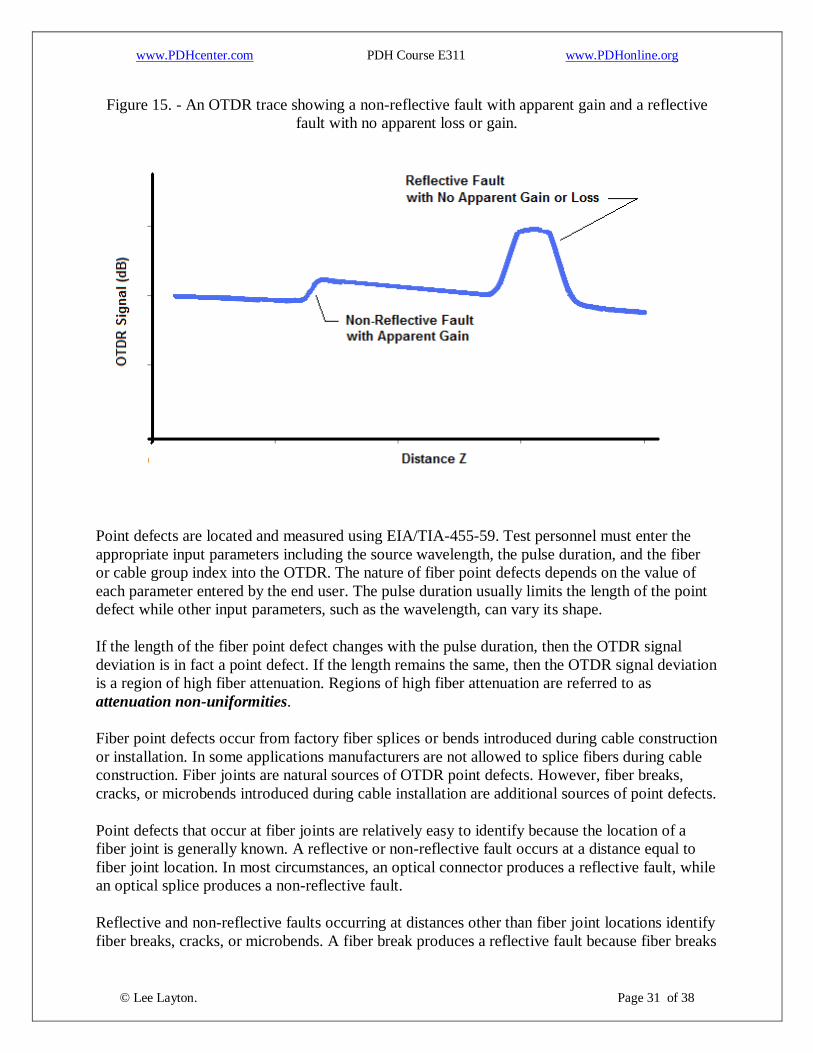
Point Defects. - Point defects are temporary or local deviations of the OTDR signal in the
upward or downward direction. A point defect, or fault, can be reflective or non-reflective. A
point defect normally exhibits a loss of optical power. However, a point defect may exhibit an
apparent power gain. In some cases, a point defect can even exhibit no loss or gain. Refer back
to Figure 13; it illustrates a reflective fault and a non-reflective fault, both exhibiting loss. Figure
15 shows a non-reflective fault with apparent gain and a reflective fault with no apparent loss or
gain.
www.PDHcenter.com PDH Course E311 www.PDHonline.org
© Lee Layton. Page 31 of 38
Figure 15. - An OTDR trace showing a non-reflective fault with apparent gain and a reflective
fault with no apparent loss or gain.
Point defects are located and measured using EIA/TIA-455-59. Test personnel must enter the
appropriate input parameters including the source wavelength, the pulse duration, and the fiber
or cable group index into the OTDR. The nature of fiber point defects depends on the value of
each parameter entered by the end user. The pulse duration usually limits the length of the point
defect while other input parameters, such as the wavelength, can vary its shape.
If the length of the fiber point defect changes with the pulse duration, then the OTDR signal
deviation is in fact a point defect. If the length remains the same, then the OTDR signal deviation
is a region of high fiber attenuation. Regions of high fiber attenuation are referred to as
attenuation non-uniformities.
Fiber point defects occur from factory fiber splices or bends introduced during cable construction
or installation. In some applications manufacturers are not allowed to splice fibers during cable
construction. Fiber joints are natural sources of OTDR point defects. However, fiber breaks,
cracks, or microbends introduced during cable installation are additional sources of point defects.
Point defects that occur at fiber joints are relatively easy to identify because the location of a
fiber joint is generally known. A reflective or non-reflective fault occurs at a distance equal to
fiber joint location. In most circumstances, an optical connector produces a reflective fault, while
an optical splice produces a non-reflective fault.
Reflective and non-reflective faults occurring at distances other than fiber joint locations identify
fiber breaks, cracks, or microbends. A fiber break produces a reflective fault because fiber breaks

www.PDHcenter.com PDH Course E311 www.PDHonline.org
© Lee Layton. Page 32 of 38
result in complete fiber separation. Fiber cracks and microbends generally produce non-reflective
faults.
A point defect may exhibit apparent gain because the backscatter coefficient of the fiber present
before the point defect is higher than that of the fiber present after. Test personnel measure the
signal loss or gain by positioning a pair of cursors, one on each side of the point defect. Figure
16 illustrates the positioning of the cursors for a point defect showing an apparent signal gain.
The trace after the point defect is extrapolated as shown in Figure 16. The vertical distance
between the two lines in Figure 16 is the apparent gain of the point defect.
Figure 16. - Extrapolation for a point defect showing an apparent signal gain.
Point defects exhibiting gain in one direction will exhibit an exaggerated loss in the opposite
direction. Figure 17 shows the apparent loss shown by the OTDR for the same point defect
shown in Figure 16 when measured in the opposite direction. Bidirectional measurements are
conducted to cancel the effects of backscatter coefficient variations. Bidirectional averaging
combines the two values to identify the true signal loss. Bidirectional averaging is possible only
if test personnel have access to both ends of the test sample.

www.PDHcenter.com PDH Course E311 www.PDHonline.org
© Lee Layton. Page 33 of 38
Figure 17. - The exaggerated loss obtained at point defects exhibiting gain in one direction by
conducting the OTDR measurement in the opposite direction.
OTDRs can also measure the return loss of a point defect. However, not all OTDRs are
configured to make the measurement. To measure the return loss of a point defect, the cursors
are placed in the same places as for measuring the loss of the point defect. The return loss of the
point defect is displayed when the return loss option is selected on the OTDR. The steps for
selecting the return loss option depend upon the OTDR being used.
Power Meter
Test personnel also use an optical power meter and stabilized light source to measure fiber
attenuation and transmission loss in the field. Optical power meter measurements are
recommended when the length of an installed optical fiber cable or cable plant is less than 50
meters. A test jumper is used to couple light from the stabilized source to one end of the optical
fiber (or cable plant) under test. An additional test jumper is also used to connect the other end of
the optical fiber (or cable plant) under test to the power meter. Optical power meter
measurements may be conducted using an optical loss test set (OLTS). An OLTS combines the
power meter and source functions into one physical unit. When making measurements, it does
not matter whether the stabilized source and power meter are in one physical unit or two.
www.PDHcenter.com PDH Course E311 www.PDHonline.org
© Lee Layton. Page 34 of 38
Power meter measurements are conducted on individual optical fiber cables installed. The
installed optical fiber cable must have connectors or terminations on both ends to make the
measurement. If the installed optical fiber cable does not have connectors or terminations on
both ends, an OTDR should be used to evaluate the cable. If the cable is too short for evaluation
with an OTDR, cable continuity can be verified using a flashlight.
Power meter measurements for cable assembly link loss require that test personnel clean all
optical connections at test jumper interfaces before performing any measurement. Test personnel
should use cotton wipes dampened with alcohol to clean connectors and blow dry before making
connections. End users should also ensure that test equipment calibration is current.
Power meter measurements are made by connecting a test reference cable between the light
source and power meter. The test reference cable has the same nominal fiber characteristics as
the cable under test. The optical power present at the power meter is the reference power (P1).
The reference cable is then disconnected and the optical fiber cable under test is connected
between the light source and power meter using test jumpers. If possible, the test reference cable
should be used as the input jumper cable for the test cable measurement. The test jumper fiber
properties, such as core diameter and NA, should be nominally equal to the fiber properties of
the cable being tested. The optical power present at the power meter is test power (P2).
Test personnel use P1 and P2 to calculate the cable assembly link loss. The cable assembly link
loss (BCA) of optical fiber installed with connectors or terminations on both ends is,
BCA = P1 – P2
Where,
BCA = Cable assembly link loss, db.
P1 = Reference power of the test cable.
P2 = Optical power of the cable under test.
The cable assembly link loss should always be less than the specified link loss for that particular
link.
Besides measuring individual cables, test personnel measure the transmission loss of installed
fiber optic cable plants. The transmission loss of fiber optic cable plants is measured using
EIA/TIA-526-14 method B (multimode fiber) or EIA/TIA-526-7 (single mode fiber). The
procedure measures the internal loss of the cable plant between points A and B, plus two
connection losses. The top view in Figure 18 illustrates the method described in EIA/TIA-526-
14 method B for measuring the reference power (P1). The bottom view in Figure 18 shows the
final test configuration for measuring the cable plant test power (P2).

www.PDHcenter.com PDH Course E311 www.PDHonline.org
© Lee Layton. Page 35 of 38
Figure 18. - EIA/TIA-526-14 methods for measuring the reference power (P1).
The procedure is exactly the same as described for measuring the link loss of an individual cable
assembly. The total optical loss between any two termination points, including the end
terminations, of the optical fiber cable plant link is measured. The measured cable plant link loss
should always be less than the specified cable plant link loss.
Test personnel should conduct cable assembly link loss, and cable plant transmission loss
measurements in both directions and at each system operational wavelength. By performing
these measurements in each direction, test personnel can better characterize cable and link losses.
Unlike optical time-domain reflectometry, bidirectional readings are always possible when
performing power meter measurements. In power meter measurements, by definition, end users
have access to both ends of the cable or cable plant.
www.PDHcenter.com PDH Course E311 www.PDHonline.org
© Lee Layton. Page 36 of 38
Summary
The following is a summary of a few of the key terms and ideas presented this course.
Laboratory measurements of the optical fiber and optical connections performed by end users in
the laboratory include attenuation, cutoff wavelength (single mode), bandwidth (multimode),
chromatic dispersion, fiber geometry, core diameter, numerical aperture (multimode), mode field
diameter (single mode), insertion loss, and reflectance and return loss.
Attenuation is the loss of optical power as light travels along the fiber. It is a result of absorption,
scattering, bending, and other loss mechanisms.
The launch spot size and the angular distribution may affect multimode fiber attenuation
measurement results by affecting modal distributions.
An underfilled launch results when the launch spot size and angular distribution are smaller than
that of the fiber core.
An overfilled launch condition occurs when the launch spot size and angular distribution are
larger than that of the fiber core.
A cladding-mode stripper is a device that removes any cladding mode power from the fiber.
A mode filter is a device that attenuates a specific mode or modes propagating in the core of an
optical fiber.
The cutoff wavelength of a single mode fiber is the wavelength above which the fiber propagates
only the fundamental mode. The cutoff wavelength of a single mode fiber varies according to the
fiber's radius of curvature and length. The fiber cutoff wavelength (cf) will generally be higher
than the cable cutoff wavelength (cc).
Pulse distortion is the spreading of the light pulse as it travels along the fiber caused by
dispersion. It reduces the bandwidth, or information-carrying capacity, of an optical fiber.
Two basic techniques are used for measuring the modal bandwidth of an optical fiber. The first
characterizes dispersion by measuring the impulse response h(t) of the fiber in the time domain.
The second characterizes modal dispersion by measuring the baseband frequency response H(f)
of the fiber in the frequency domain.
The lowest frequency at which the magnitude of the fiber frequency response has decreased to
one half its zero-frequency value is the -3 decibel (db) optical power frequency ( f3db).
Chromatic dispersion occurs because different colors of light travel through the fiber at different
speeds. Since the different colors of light have different velocities, some colors arrive at the fiber
end before others.
www.PDHcenter.com PDH Course E311 www.PDHonline.org
© Lee Layton. Page 37 of 38
The differential group delay () is the variation in propagation delay that occurs because of the
different group velocities of each wavelength in an optical fiber.
The range of wavelengths over which meaningful chromatic dispersion data is obtained depends
on the wavelength range of optical source(s) used.
Fiber geometry measurements are performed by end users to reduce system attenuation and
coupling loss resulting from poor fiber fabrication.
The cladding diameter is the average diameter of the cladding.
Cladding non-circularity, or ellipticity, is the difference between the smallest radius of the fiber
(rgmin) and the largest radius of the fiber (rgmax) divided by the average cladding radius (rg).
The core-cladding concentricity error for multimode fibers is the distance between the core and
cladding centers divided by the core diameter. The core-cladding concentricity error for single
mode fibers is defined as the distance between the core and cladding centers.
Core non-circularity is the difference between the smallest radius of the core (rcmin) and the
largest radius of the core (rcmax) divided by the core radius (rc).
The near-field power distribution is defined as the emitted power per unit area (radiance) for
each position in the plane of the emitting surface.
The near-field region is the region close to the fiber-end face.
The core diameter is derived from the normalized output near-field radiation pattern. The core
diameter (d) is defined as the diameter at the 2.5 percent (0.025) level.
The numerical aperture (NA) is a measurement of the ability of a multimode optical fiber to
capture light.
The far-field power distribution describes the emitted power per unit area as a function of angle
some distance away from the fiber-end face.
The far-field region is the region far from the fiber-end face.
Single mode fibers with large mode field diameters are more sensitive to fiber bending. Single
mode fibers with small mode field diameters show higher coupling losses at connections.
Insertion loss is composed of the connection coupling loss and additional fiber losses in the fiber
following the connection.
Reflectance is a measure of the portion of incident light that is reflected back into the source
fiber at the point of connection.
www.PDHcenter.com PDH Course E311 www.PDHonline.org
© Lee Layton. Page 38 of 38
Return loss is the amount of loss of the reflected light compared with the power of the incident
beam at the interface.
Optical fiber and optical connection field measurements measure only the transmission
properties affected by component or system installation or repair.
Optical time-domain reflectometry is recommended for conducting field measurements on
installed optical fibers or cable plants of 50 meters or more in length.
An optical loss test set (OLTS) combines the power meter and source functions into one physical
unit.
An optical time-domain reflectometer (OTDR) measures the fraction of light that is reflected
back because of Rayleigh scattering and Fresnel reflection.
A fiber optic cable plant consists of optical fiber cables, connectors, splices, mounting panels,
jumper cables, and other passive components. A cable plant does not include active components
such as optical transmitters or receivers.
A point defect is a temporary or permanent local deviation of the OTDR signal in the upward or
downward direction. Point defects are caused by connectors, splices, or fiber breaks. Point
defects, or faults, can be reflective or non-reflective.
A dead-zone fiber is placed between the test fiber and OTDR to reduce the influence of the
initial pulse resulting from Fresnel reflection at the OTDR connection.
The amount of optical power backscattered because of Rayleigh scattering at one point depends
on the forward optical power and the fibers backscatter capture coefficient.
The effects of backscatter variations can be eliminated by test personnel by performing the
OTDR attenuation measurement in each direction along the test fiber and averaging
(bidirectional readings).
A point defect may exhibit apparent gain because the backscatter coefficient of the fiber present
before the point defect is higher than that of the fiber present after.
To measure fiber attenuation and transmission loss in the field, test personnel use an optical
power meter and stabilized light source.
Optical power meter measurements are recommended when the length of an installed optical
fiber cable or cable plant is less than 50 meters.
+++