fft - california state university channel...
TRANSCRIPT
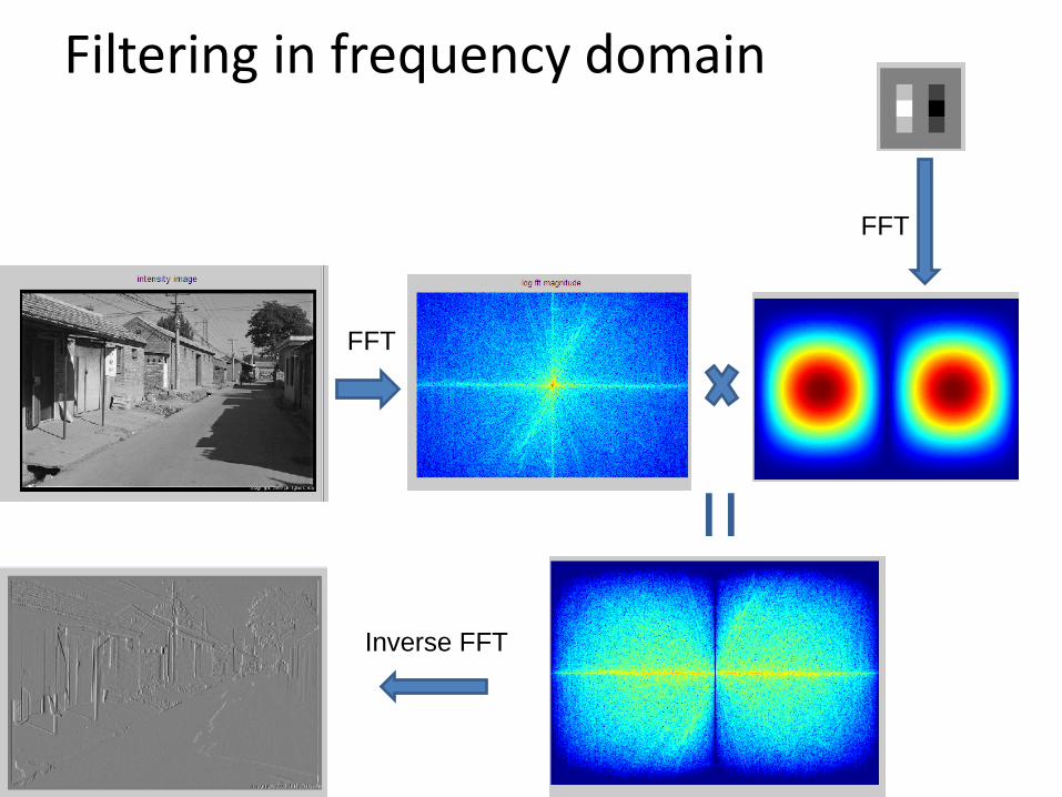
Filtering in frequency domain
FFT
FFT
Inverse FFT
=
• Filtering in frequency domain – Can be faster than filtering in spatial domain (for
large filters) – Can help understand effect of filter – Algorithm:
1. Convert image and filter to fft (fft2 in matlab) 2. Pointwise-multiply ffts 3. Convert result to spatial domain with ifft2
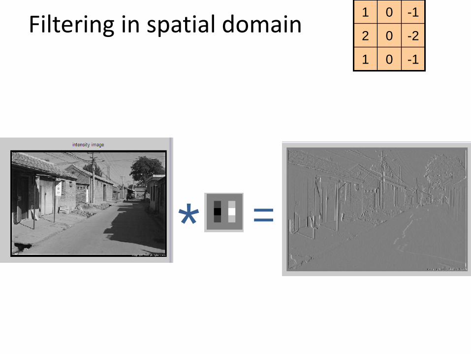
Filtering in spatial domain -1 0 1
-2 0 2
-1 0 1
* =
• Filtering in spatial domain – Slide filter over image and take dot product at
each position – Remember linearity (for linear filters) – Examples
• 2D: [1 0 0 ; 0 2 0 ; 0 0 1]/4
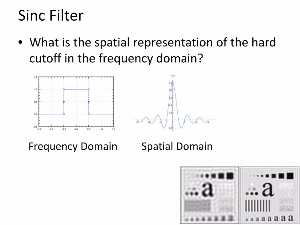
• What is the spatial representation of the hard cutoff in the frequency domain?
Sinc Filter
Frequency Domain Spatial Domain
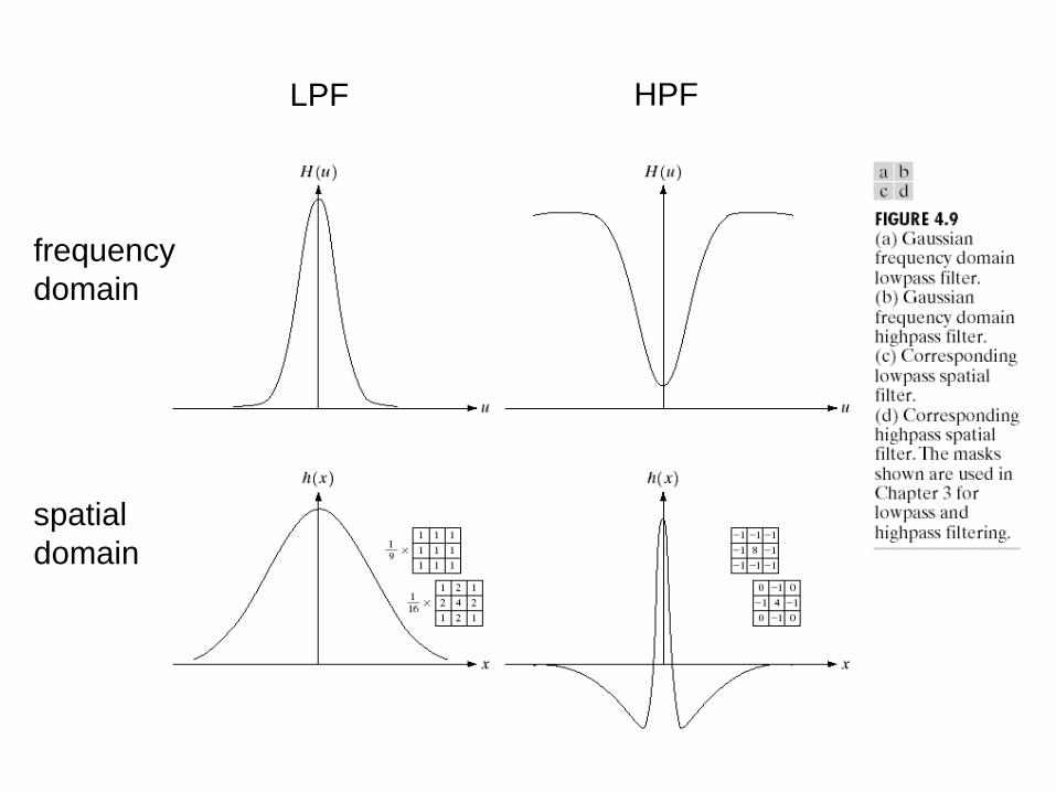
LPF HPF
frequency domain
spatial domain
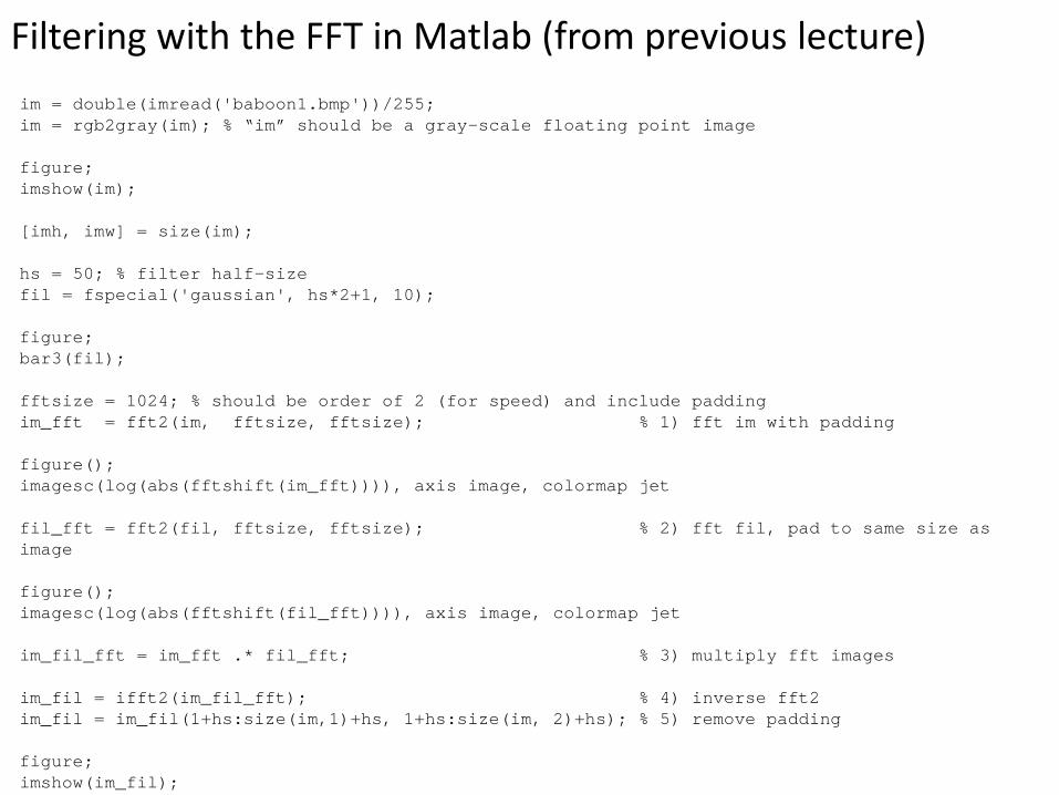
Filtering with the FFT in Matlab (from previous lecture) im = double(imread('baboon1.bmp'))/255; im = rgb2gray(im); % “im” should be a gray-scale floating point image figure; imshow(im); [imh, imw] = size(im); hs = 50; % filter half-size fil = fspecial('gaussian', hs*2+1, 10); figure; bar3(fil); fftsize = 1024; % should be order of 2 (for speed) and include padding im_fft = fft2(im, fftsize, fftsize); % 1) fft im with padding figure(); imagesc(log(abs(fftshift(im_fft)))), axis image, colormap jet fil_fft = fft2(fil, fftsize, fftsize); % 2) fft fil, pad to same size as image figure(); imagesc(log(abs(fftshift(fil_fft)))), axis image, colormap jet im_fil_fft = im_fft .* fil_fft; % 3) multiply fft images im_fil = ifft2(im_fil_fft); % 4) inverse fft2 im_fil = im_fil(1+hs:size(im,1)+hs, 1+hs:size(im, 2)+hs); % 5) remove padding figure; imshow(im_fil);
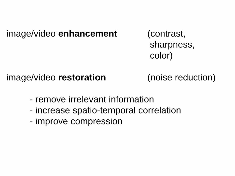
image/video enhancement (contrast, sharpness, color) image/video restoration (noise reduction) - remove irrelevant information - increase spatio-temporal correlation - improve compression
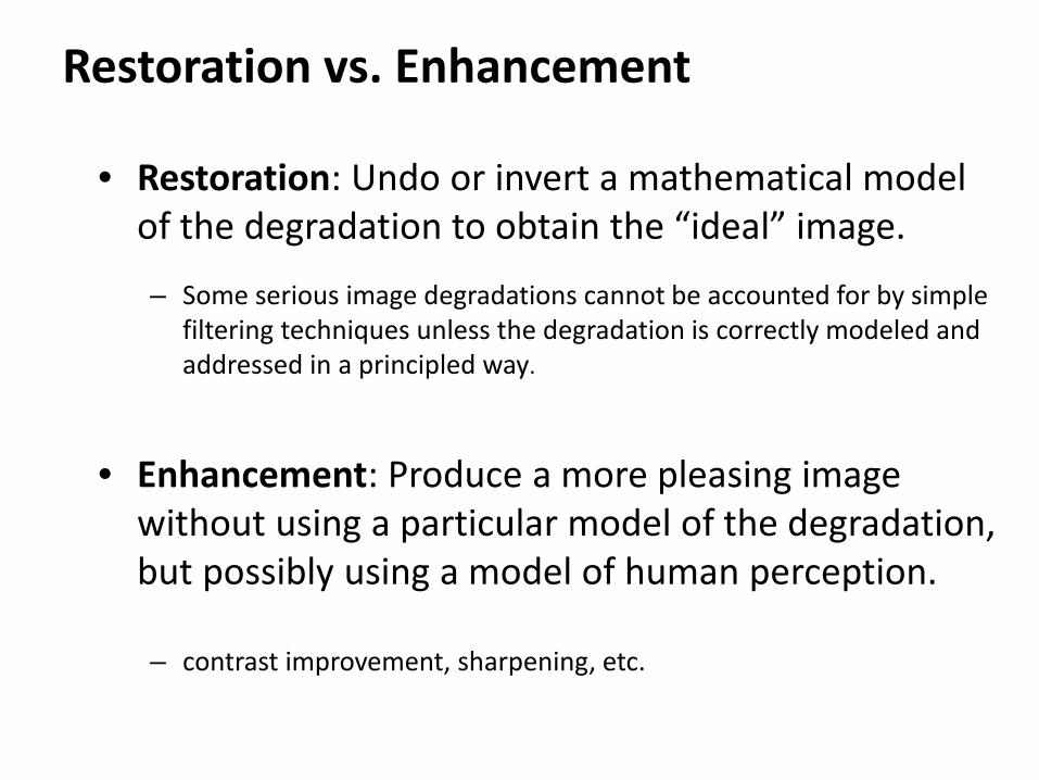
Restoration vs. Enhancement
• Restoration: Undo or invert a mathematical model of the degradation to obtain the “ideal” image.
– Some serious image degradations cannot be accounted for by simple filtering techniques unless the degradation is correctly modeled and addressed in a principled way.
• Enhancement: Produce a more pleasing image
without using a particular model of the degradation, but possibly using a model of human perception.
– contrast improvement, sharpening, etc.
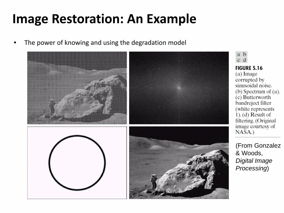
Image Restoration: An Example • The power of knowing and using the degradation model
(From Gonzalez & Woods, Digital Image Processing)
Noise: random unwanted portion of signal/data without meaning; an unwanted by-product of other activities.
Image noise: random variation of brightness or color in images; usually an aspect of electronic noise.
Gaussian noise: caused primarily by thermal noise in amplifier circuitry of camera Salt and Pepper noise: caused by analog-to-digital converter errors, bit errors in transmission Shot noise: variation in the number of photons sensed at a given exposure level Film grain: due to the grain of photographic film
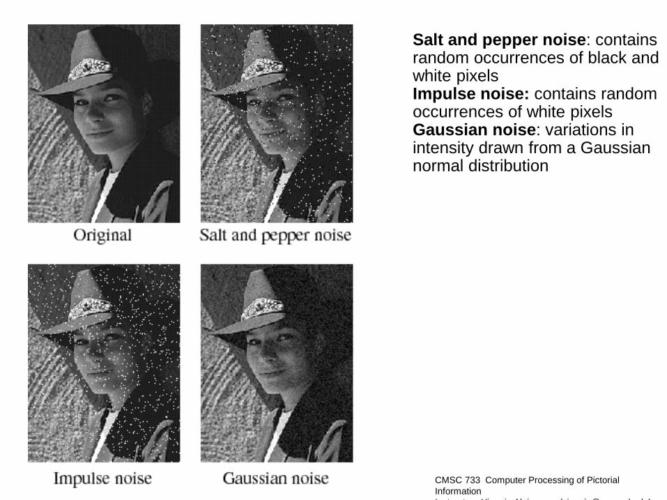
Salt and pepper noise: contains random occurrences of black and white pixels Impulse noise: contains random occurrences of white pixels Gaussian noise: variations in intensity drawn from a Gaussian normal distribution
CMSC 733 Computer Processing of Pictorial Information I t t Yi i Al i ( i i @ d d )
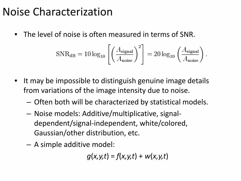
Noise Characterization
• The level of noise is often measured in terms of SNR.
• It may be impossible to distinguish genuine image details from variations of the image intensity due to noise. – Often both will be characterized by statistical models. – Noise models: Additive/multiplicative, signal-
dependent/signal-independent, white/colored, Gaussian/other distribution, etc.
– A simple additive model: g(x,y,t) = f(x,y,t) + w(x,y,t)
linear filters - mean, average, box filters - Gaussian filters order-statistic filters - median filters multiresolution filters
Noise Filters
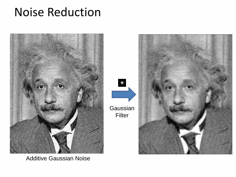
Noise Reduction
Additive Gaussian Noise
Gaussian Filter
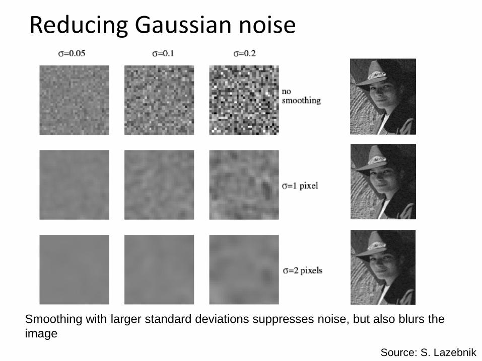
Smoothing with larger standard deviations suppresses noise, but also blurs the image
Reducing Gaussian noise
Source: S. Lazebnik
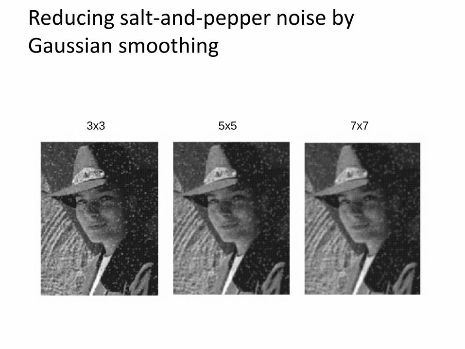
Reducing salt-and-pepper noise by Gaussian smoothing
3x3 5x5 7x7
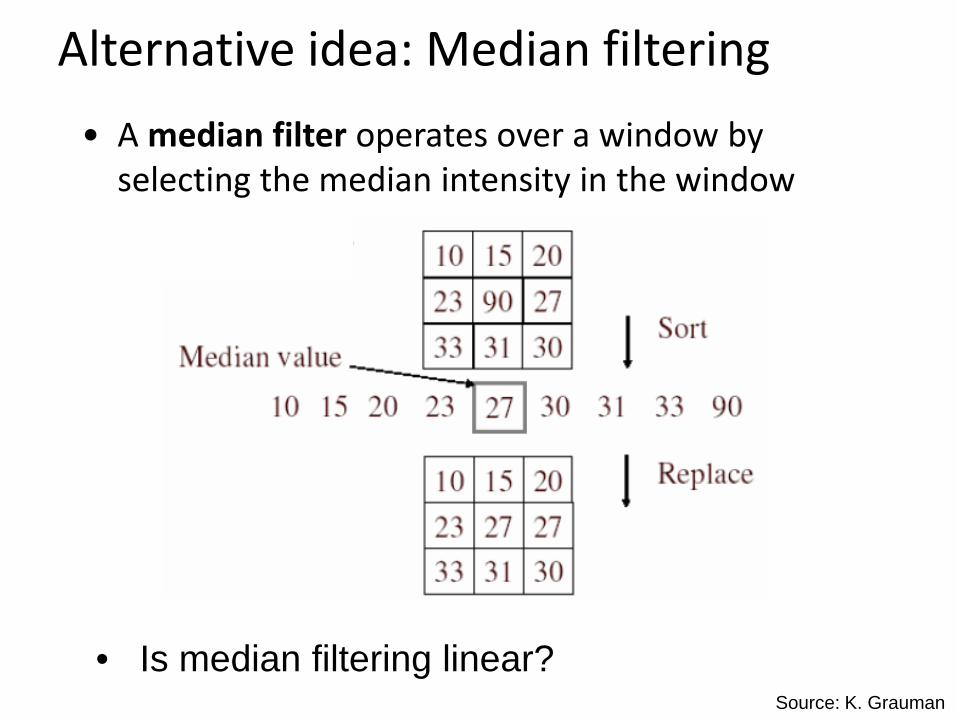
Alternative idea: Median filtering • A median filter operates over a window by
selecting the median intensity in the window
• Is median filtering linear? Source: K. Grauman
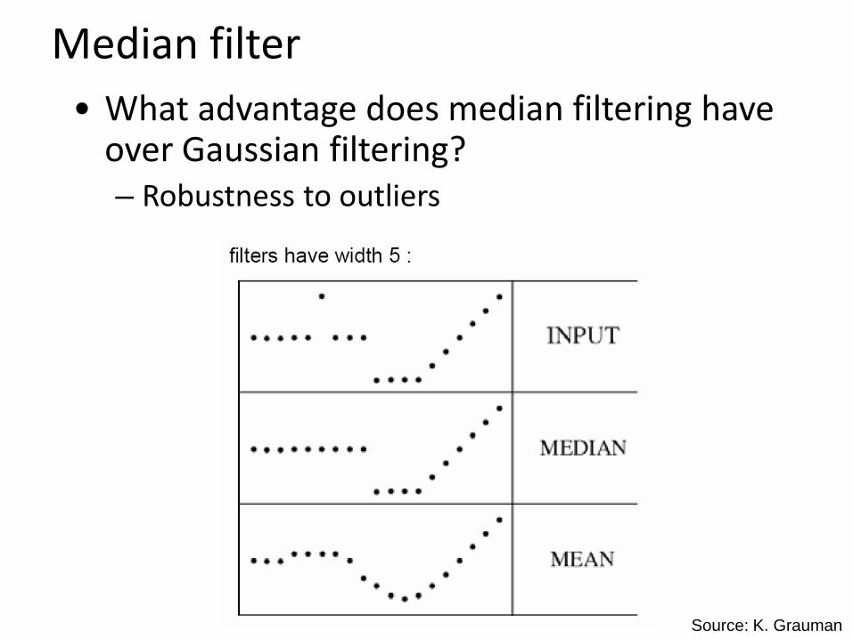
Median filter • What advantage does median filtering have
over Gaussian filtering? – Robustness to outliers
Source: K. Grauman
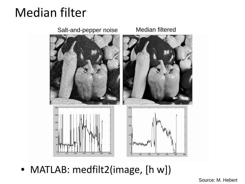
Median filter Salt-and-pepper noise Median filtered
Source: M. Hebert
• MATLAB: medfilt2(image, [h w])
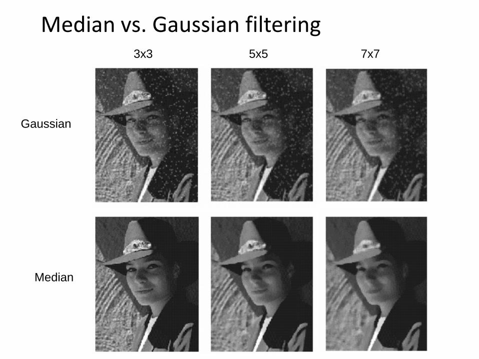
Median vs. Gaussian filtering 3x3 5x5 7x7
Gaussian
Median
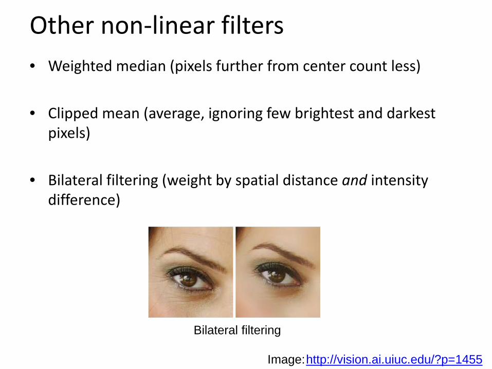
Other non-linear filters • Weighted median (pixels further from center count less)
• Clipped mean (average, ignoring few brightest and darkest
pixels)
• Bilateral filtering (weight by spatial distance and intensity difference)
http://vision.ai.uiuc.edu/?p=1455 Image:
Bilateral filtering
How is it that a 4MP image can be compressed to a few hundred KB without a noticeable change?
Compression
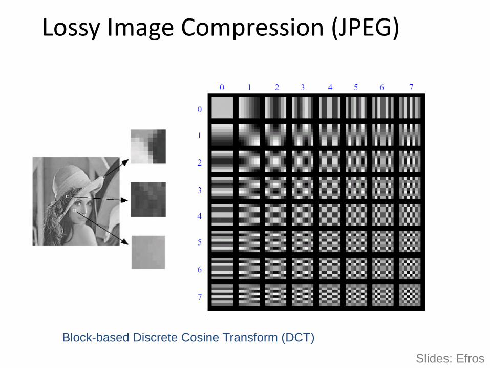
Lossy Image Compression (JPEG)
Block-based Discrete Cosine Transform (DCT)
Slides: Efros
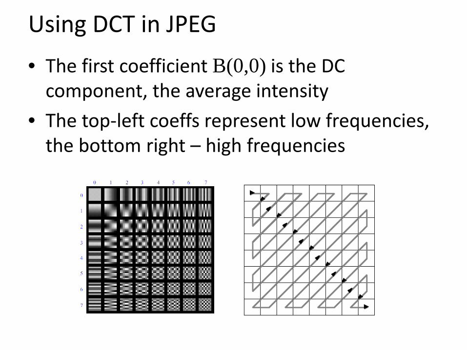
Using DCT in JPEG • The first coefficient B(0,0) is the DC
component, the average intensity • The top-left coeffs represent low frequencies,
the bottom right – high frequencies
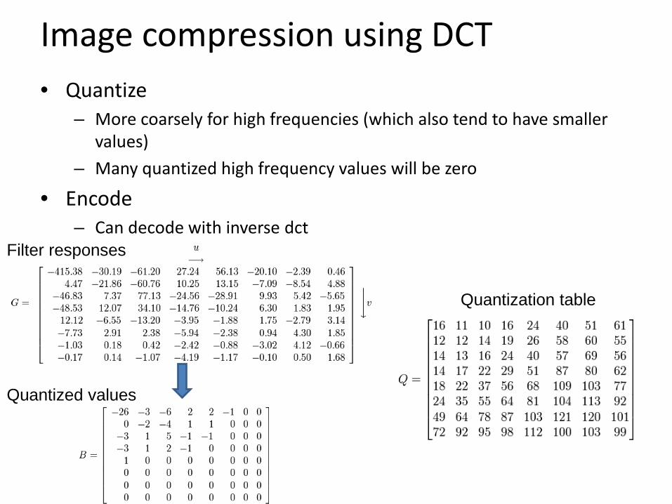
Image compression using DCT • Quantize
– More coarsely for high frequencies (which also tend to have smaller values)
– Many quantized high frequency values will be zero
• Encode – Can decode with inverse dct
Quantization table
Filter responses
Quantized values
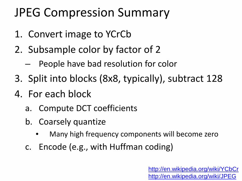
JPEG Compression Summary 1. Convert image to YCrCb 2. Subsample color by factor of 2
– People have bad resolution for color
3. Split into blocks (8x8, typically), subtract 128 4. For each block
a. Compute DCT coefficients b. Coarsely quantize
• Many high frequency components will become zero
c. Encode (e.g., with Huffman coding)
http://en.wikipedia.org/wiki/YCbCr http://en.wikipedia.org/wiki/JPEG
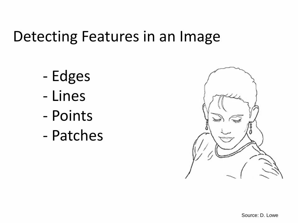
Detecting Features in an Image - Edges - Lines - Points - Patches
Source: D. Lowe
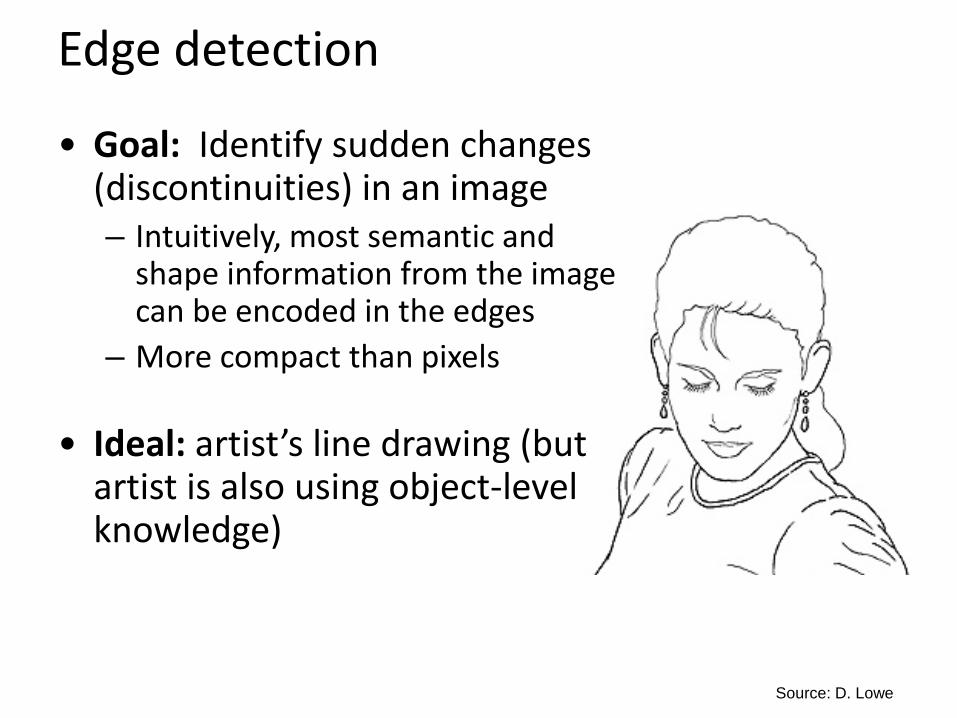
Edge detection
• Goal: Identify sudden changes (discontinuities) in an image – Intuitively, most semantic and
shape information from the image can be encoded in the edges
– More compact than pixels
• Ideal: artist’s line drawing (but artist is also using object-level knowledge)
Source: D. Lowe
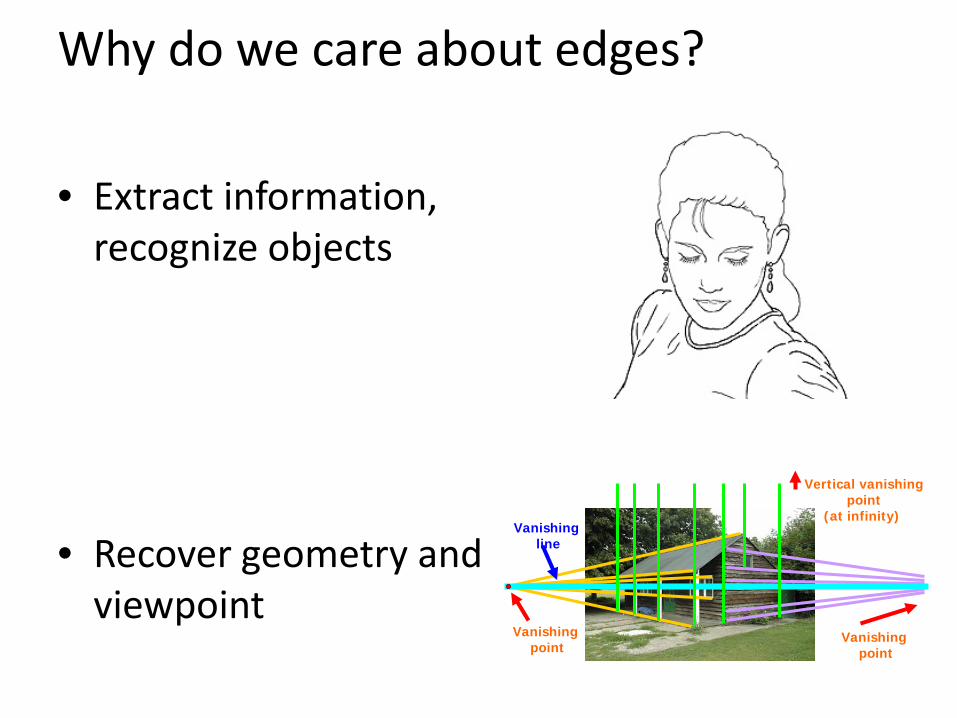
Why do we care about edges?
• Extract information, recognize objects
• Recover geometry and viewpoint
Vanishing point
Vanishing line
Vanishing point
Vertical vanishing point
(at infinity)
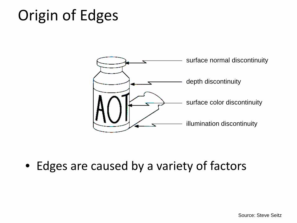
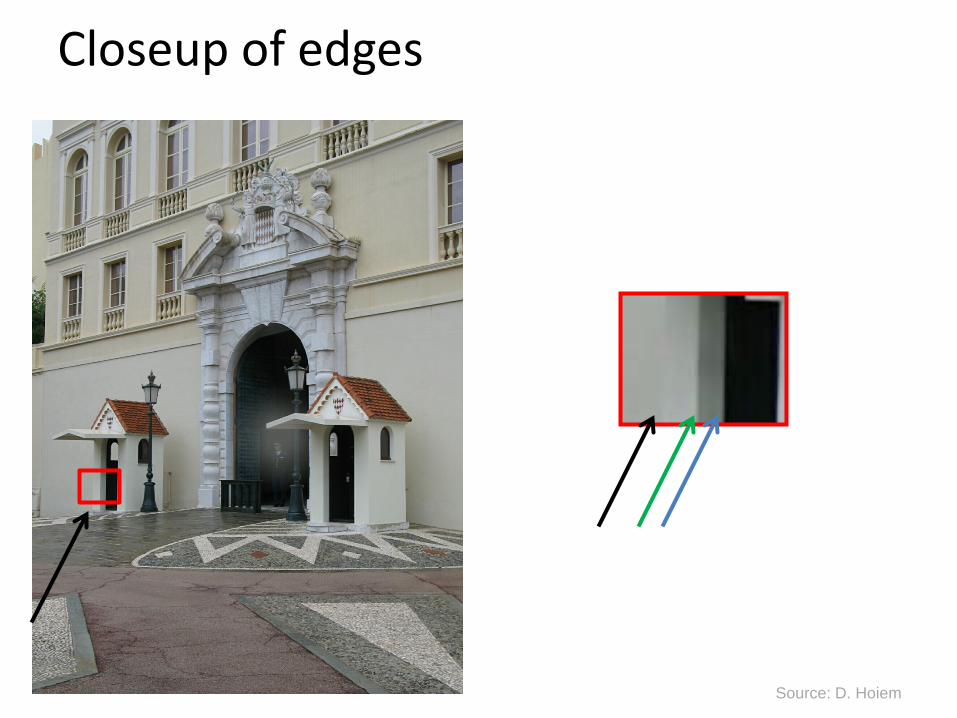
Origin of Edges
• Edges are caused by a variety of factors
depth discontinuity
surface color discontinuity
illumination discontinuity
surface normal discontinuity
Source: Steve Seitz
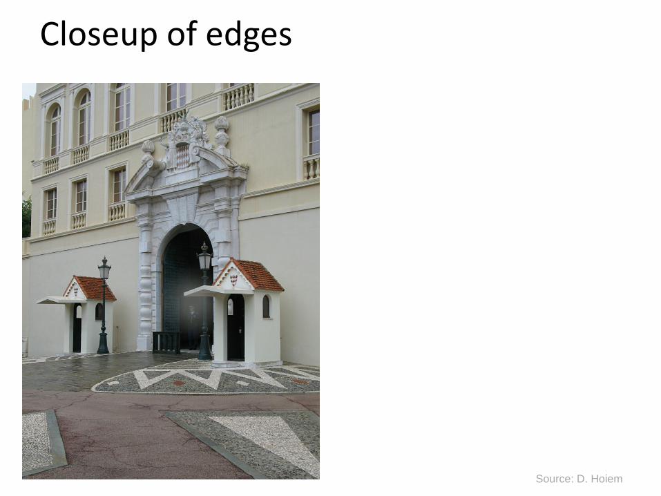
Closeup of edges
Source: D. Hoiem
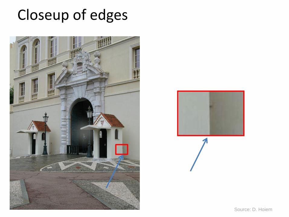
Closeup of edges
Source: D. Hoiem
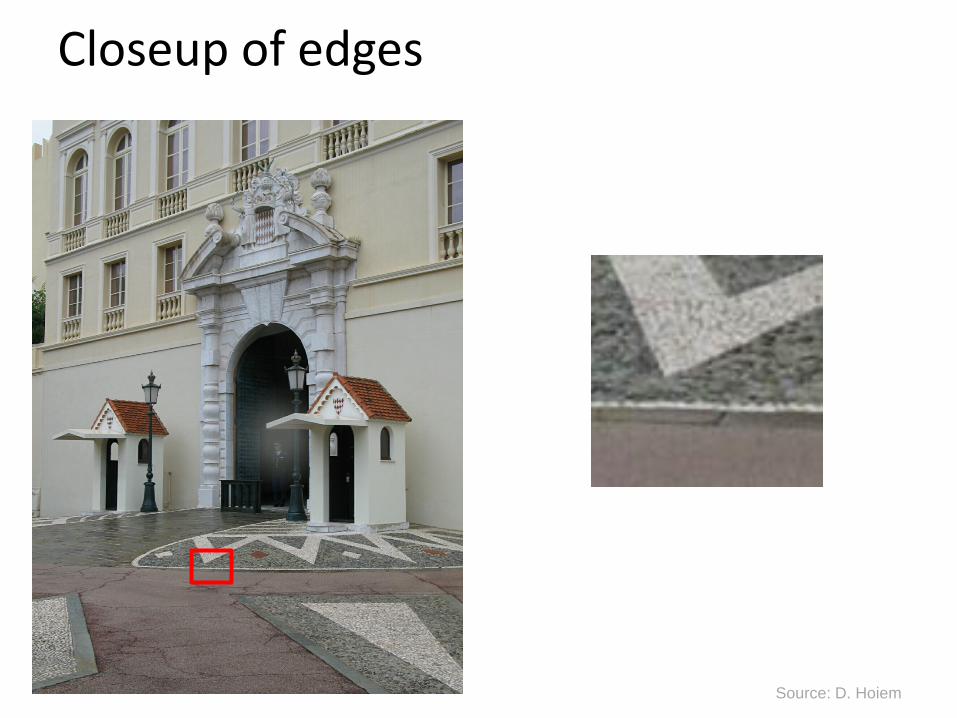
Closeup of edges
Source: D. Hoiem
Closeup of edges
Source: D. Hoiem
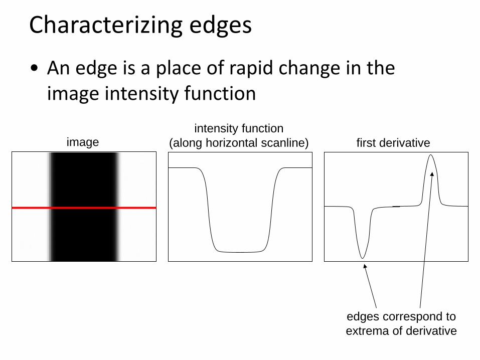
Characterizing edges • An edge is a place of rapid change in the
image intensity function
image intensity function
(along horizontal scanline) first derivative
edges correspond to extrema of derivative
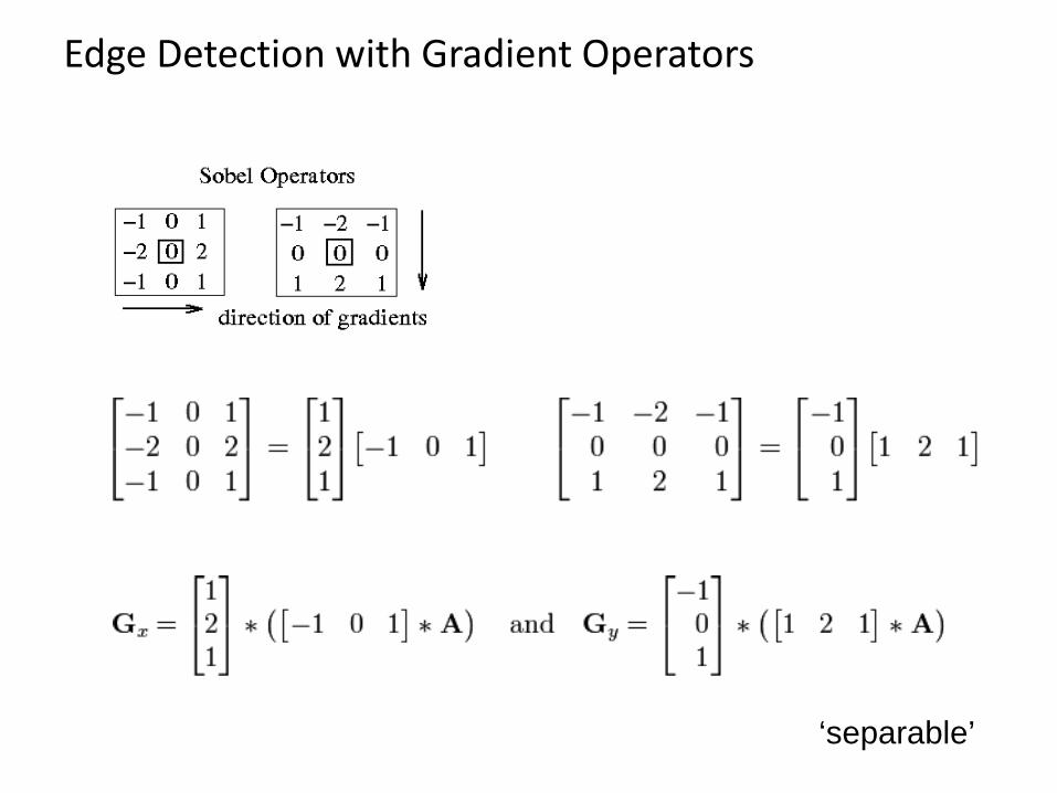
Edge Detection with Gradient Operators
‘separable’
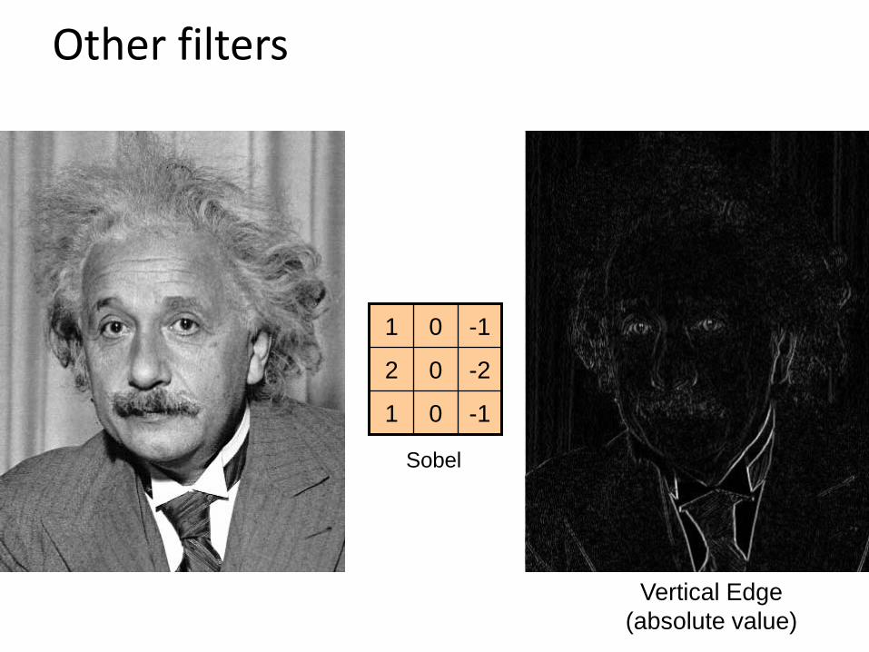
Other filters
-1 0 1
-2 0 2
-1 0 1
Vertical Edge (absolute value)
Sobel
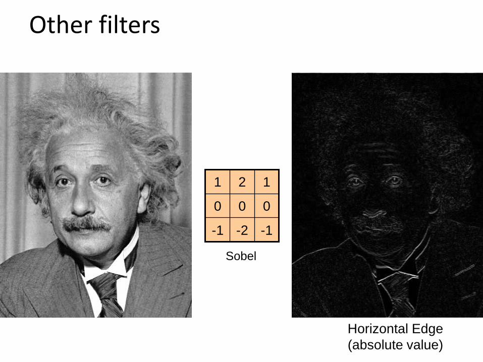
Other filters
-1 -2 -1
0 0 0
1 2 1
Horizontal Edge (absolute value)
Sobel
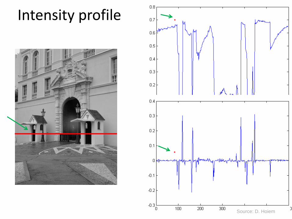
Intensity profile
Source: D. Hoiem
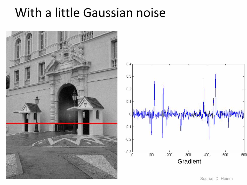
With a little Gaussian noise
Gradient
Source: D. Hoiem
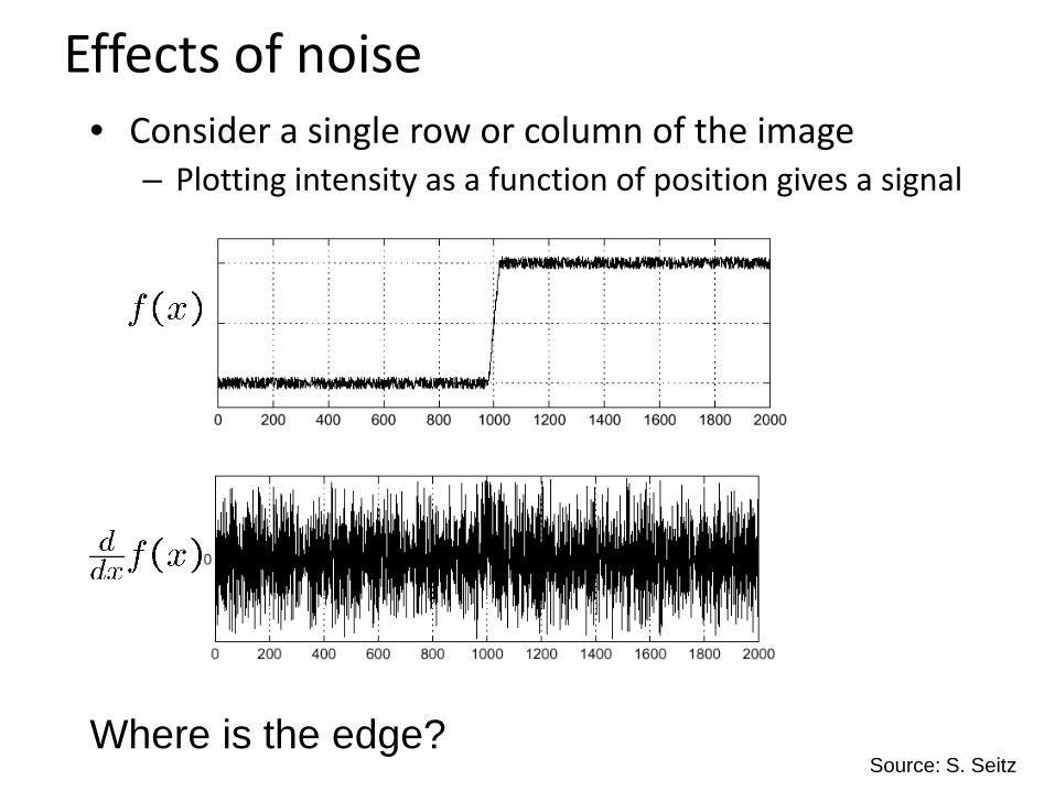
Effects of noise • Consider a single row or column of the image
– Plotting intensity as a function of position gives a signal
Where is the edge? Source: S. Seitz
Effects of noise • Difference filters respond strongly to noise
– Image noise results in pixels that look very different from their neighbors
– Generally, the larger the noise the stronger the response
• What can we do about it?
Source: D. Forsyth
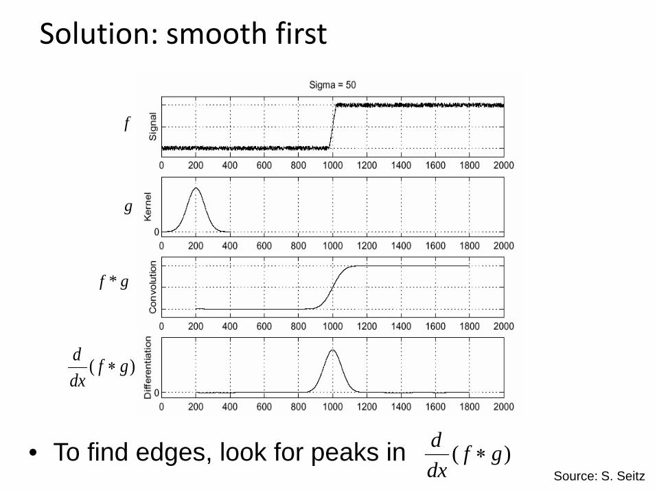
Solution: smooth first
• To find edges, look for peaks in )( gfdxd
∗
f
g
f * g
)( gfdxd
∗
Source: S. Seitz
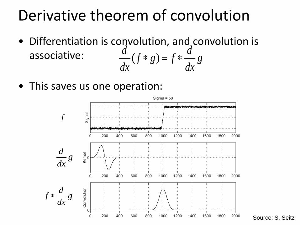
• Differentiation is convolution, and convolution is associative:
• This saves us one operation:
gdxdfgf
dxd
∗=∗ )(
Derivative theorem of convolution
gdxdf ∗
f
gdxd
Source: S. Seitz
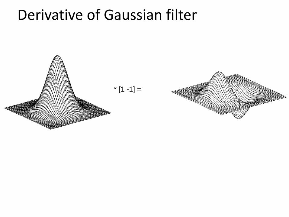
Derivative of Gaussian filter
* [1 -1] =
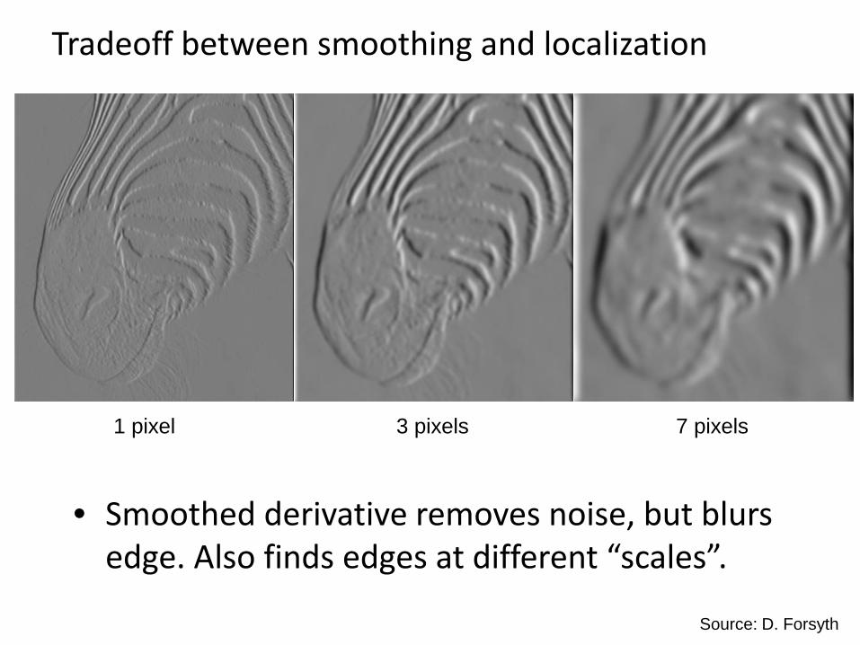
• Smoothed derivative removes noise, but blurs edge. Also finds edges at different “scales”.
1 pixel 3 pixels 7 pixels
Tradeoff between smoothing and localization
Source: D. Forsyth
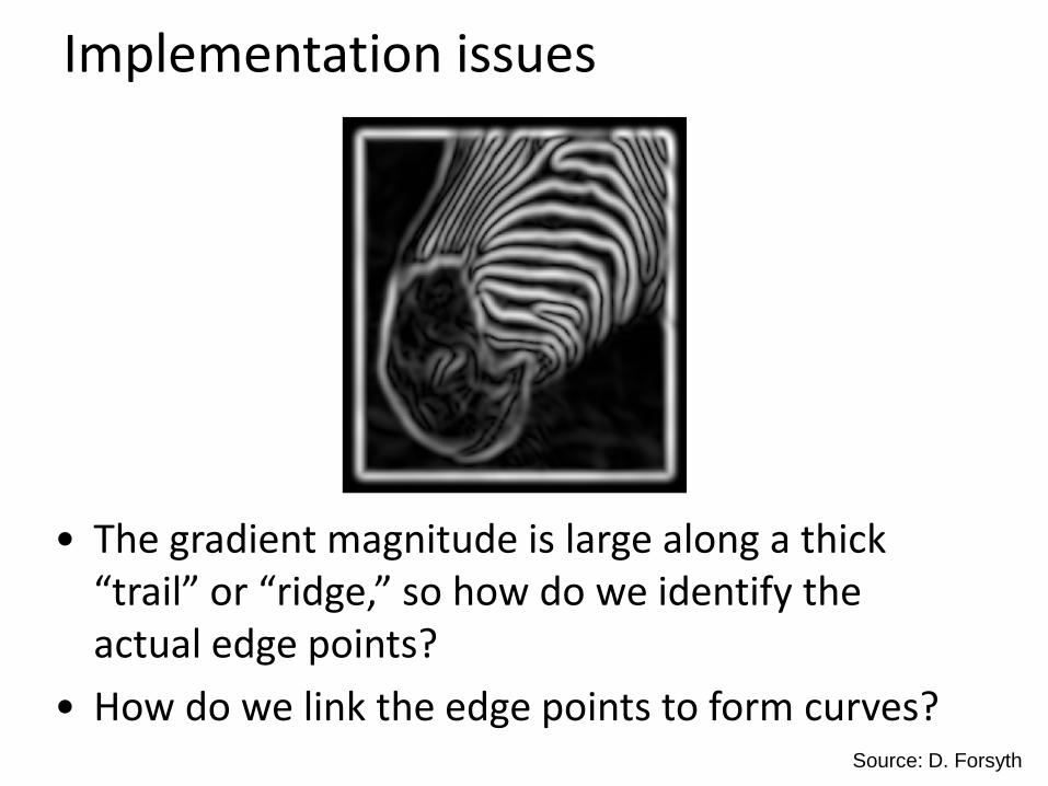
• The gradient magnitude is large along a thick “trail” or “ridge,” so how do we identify the actual edge points?
• How do we link the edge points to form curves?
Implementation issues
Source: D. Forsyth
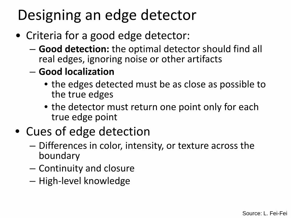
Designing an edge detector • Criteria for a good edge detector:
– Good detection: the optimal detector should find all real edges, ignoring noise or other artifacts
– Good localization • the edges detected must be as close as possible to
the true edges • the detector must return one point only for each
true edge point • Cues of edge detection
– Differences in color, intensity, or texture across the boundary
– Continuity and closure – High-level knowledge
Source: L. Fei-Fei
Slide 50 © 2007 Texas Instruments Inc,
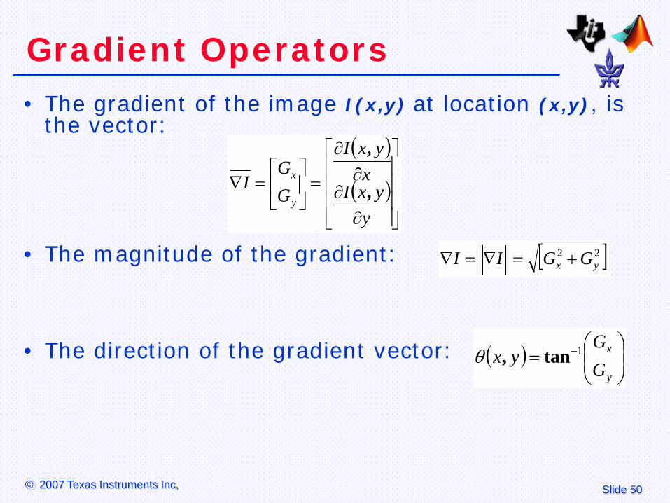
Gradient Operators • The gradient of the image I(x,y) at location (x,y), is
the vector:
• The magnitude of the gradient:
• The direction of the gradient vector:
( )
( )
∂∂∂
∂
=
=∇
yyxI
xyxI
GG
Iy
x
,
,
[ ]22yx GGII +=∇=∇
( )
= −
y
x
GG
yx 1tan,θ
Slide 51 © 2007 Texas Instruments Inc,
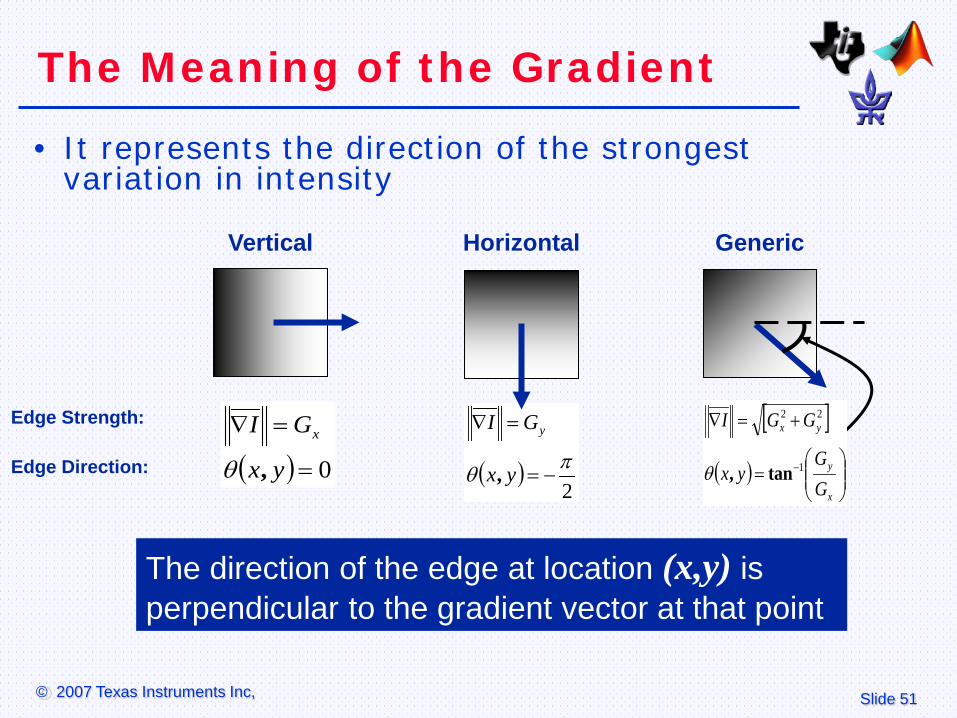
The Meaning of the Gradient
• It represents the direction of the strongest variation in intensity
( ) 0=
=∇
yx
GI x
,θ
The direction of the edge at location (x,y) is perpendicular to the gradient vector at that point
( )2πθ −=
=∇
yx
GI y
,
Vertical Horizontal Generic
Edge Strength:
Edge Direction:
[ ]
( )
=
+=∇
−
x
y
yx
GG
yx
GGI
1
22
tan,θ
Slide 52 © 2007 Texas Instruments Inc,
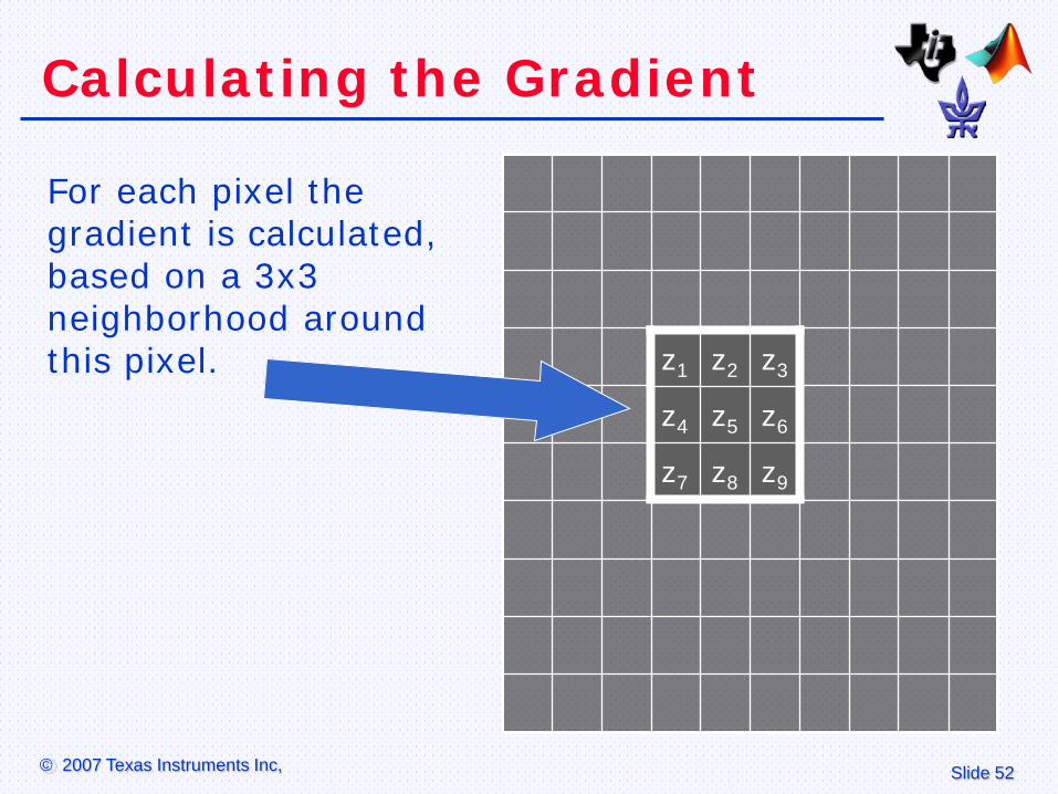
Calculating the Gradient
For each pixel the gradient is calculated, based on a 3x3 neighborhood around this pixel. z1 z2 z3
z4 z5 z6
z7 z8 z9
Slide 53 © 2007 Texas Instruments Inc,
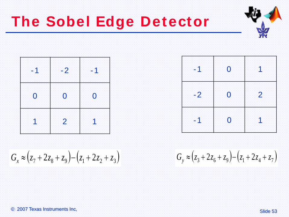
The Sobel Edge Detector
-1 -2 -1
0 0 0
1 2 1
-1 0 1
-2 0 2
-1 0 1
( ) ( )321987 22 zzzzzzGx ++−++≈ ( ) ( )741963 22 zzzzzzGy ++−++≈
Slide 54 © 2007 Texas Instruments Inc,
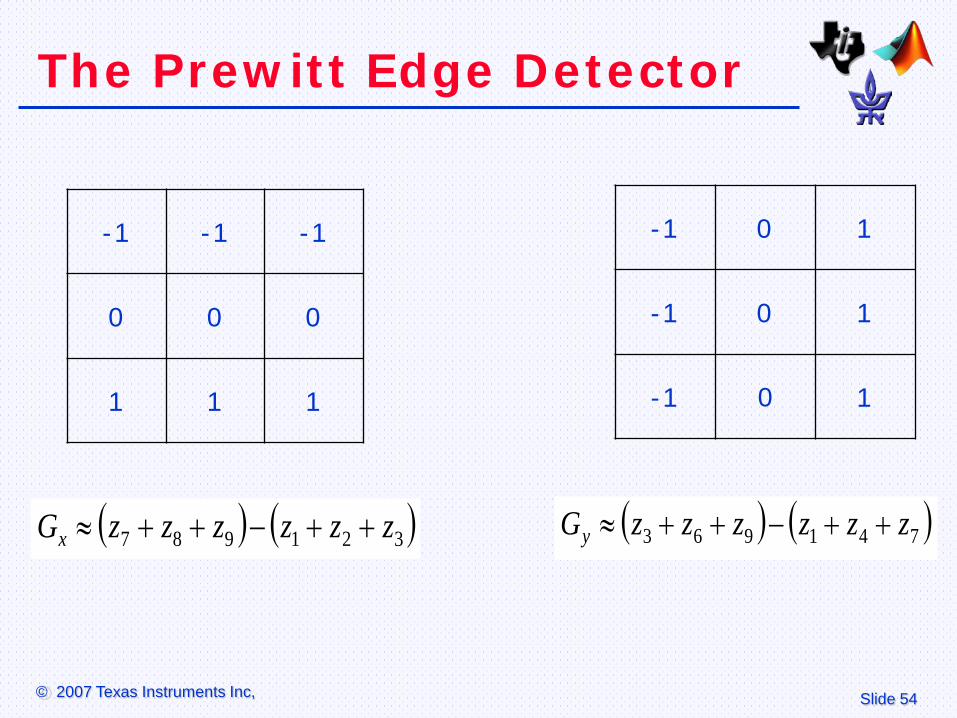
The Prewitt Edge Detector
-1 -1 -1
0 0 0
1 1 1
-1 0 1
-1 0 1
-1 0 1
( ) ( )321987 zzzzzzGx ++−++≈ ( ) ( )741963 zzzzzzGy ++−++≈
Slide 55 © 2007 Texas Instruments Inc,
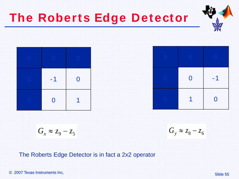
The Roberts Edge Detector
0 0 0
0 -1 0
0 0 1
0 0 0
0 0 -1
0 1 0
59 zzGx −≈ 68 zzGy −≈
The Roberts Edge Detector is in fact a 2x2 operator
Slide 56 © 2007 Texas Instruments Inc,
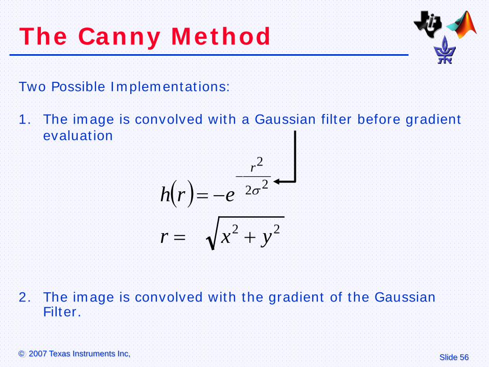
The Canny Method
Two Possible Implementations:
1. The image is convolved with a Gaussian filter before gradient evaluation
2. The image is convolved with the gradient of the Gaussian Filter.
( )22
22
2
yxr
erhr
+=
−=−
σ
Slide 57 © 2007 Texas Instruments Inc,
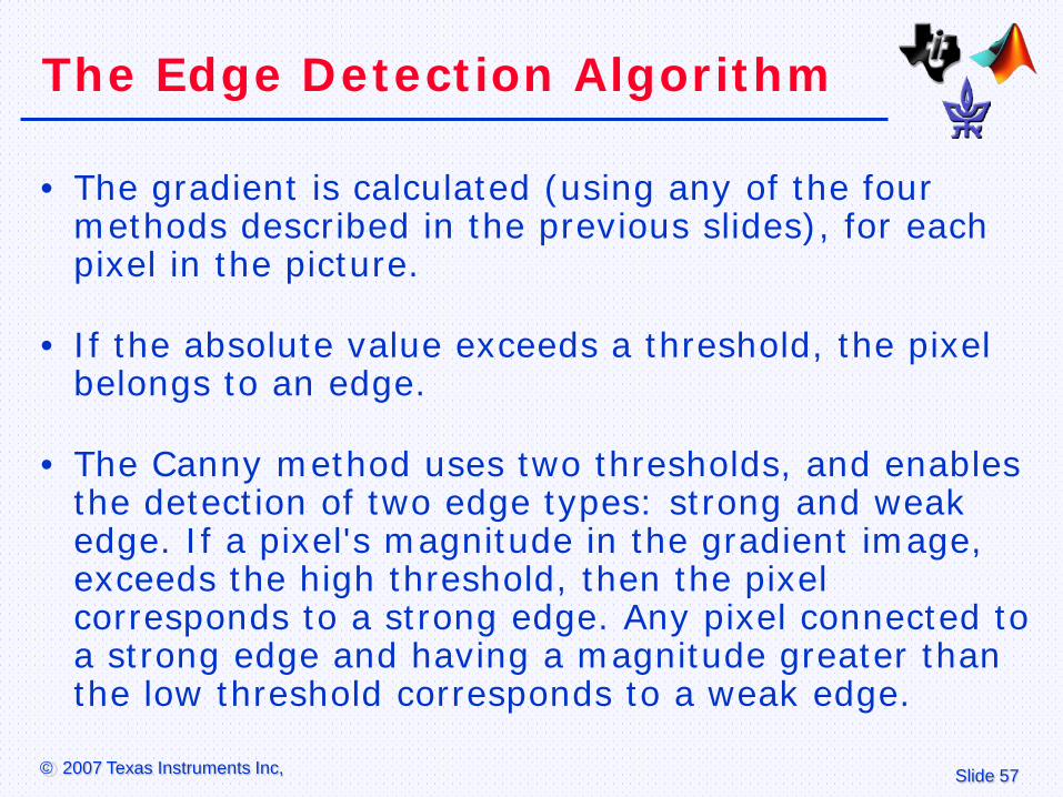
The Edge Detection Algorithm
• The gradient is calculated (using any of the four methods described in the previous slides), for each pixel in the picture.
• If the absolute value exceeds a threshold, the pixel belongs to an edge.
• The Canny method uses two thresholds, and enables the detection of two edge types: strong and weak edge. If a pixel's magnitude in the gradient image, exceeds the high threshold, then the pixel corresponds to a strong edge. Any pixel connected to a strong edge and having a magnitude greater than the low threshold corresponds to a weak edge.
Canny edge detector
• This is probably the most widely used edge detector in computer vision
• Theoretical model: step-edges corrupted by additive Gaussian noise
• Canny has shown that the first derivative of the Gaussian closely approximates the operator that optimizes the product of signal-to-noise ratio and localization
J. Canny, A Computational Approach To Edge Detection, IEEE Trans. Pattern Analysis and Machine Intelligence, 8:679-714, 1986.
Source: L. Fei-Fei
Note about Matlab’s Canny detector • Small errors in implementation
– Gaussian function not properly normalized – First filters with a Gaussian, then a difference of
Gaussian (equivalent to filtering with a larger Gaussian and taking difference)
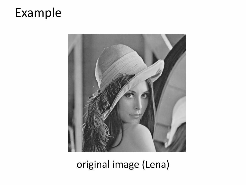
Example
original image (Lena)
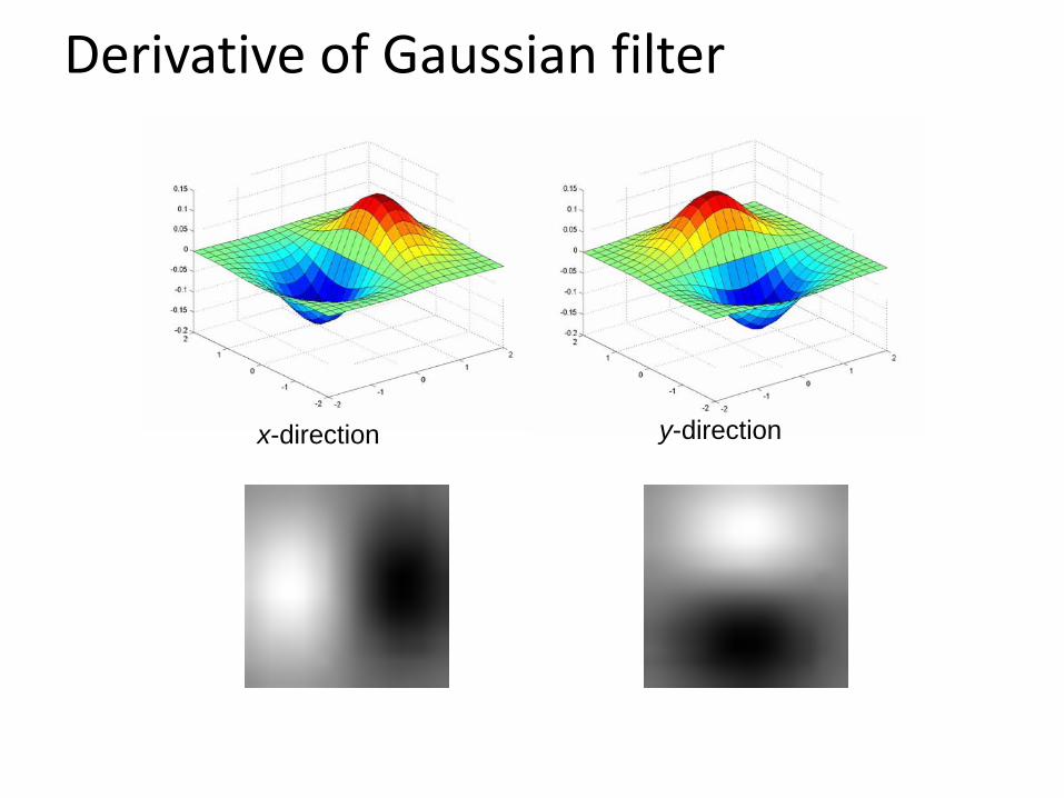
Derivative of Gaussian filter
x-direction y-direction
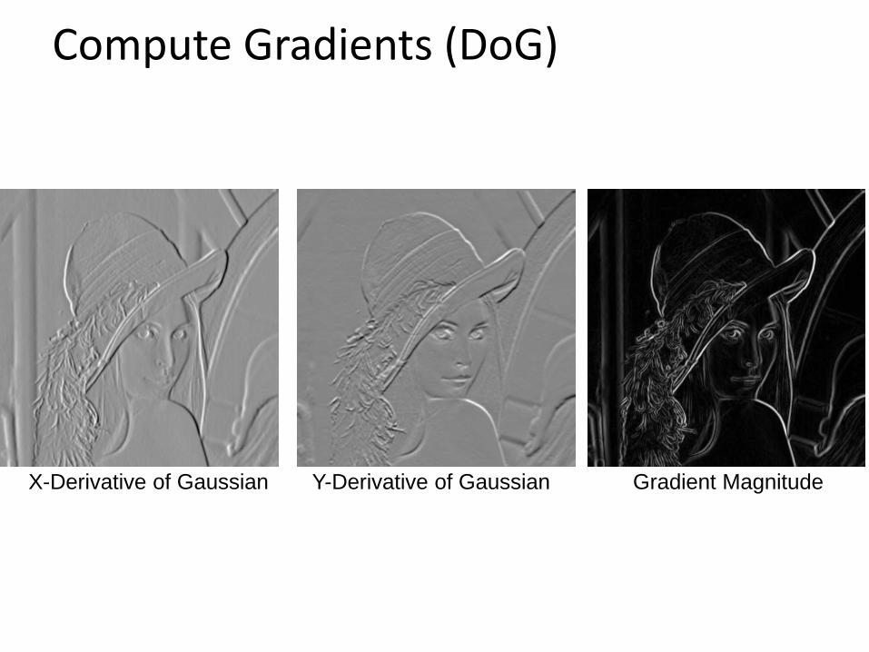
Compute Gradients (DoG)
X-Derivative of Gaussian Y-Derivative of Gaussian Gradient Magnitude

Get Orientation at Each Pixel • Threshold at minimum level • Get orientation
theta = atan2(gy, gx)
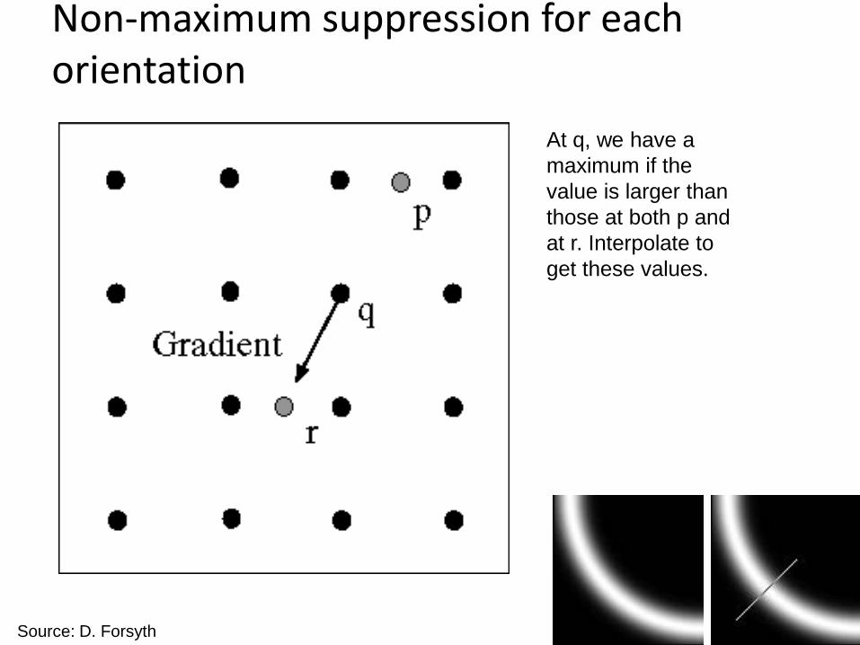
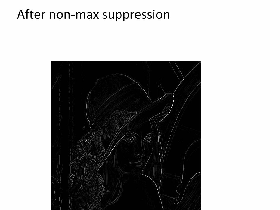
Non-maximum suppression for each orientation
At q, we have a maximum if the value is larger than those at both p and at r. Interpolate to get these values.
Source: D. Forsyth
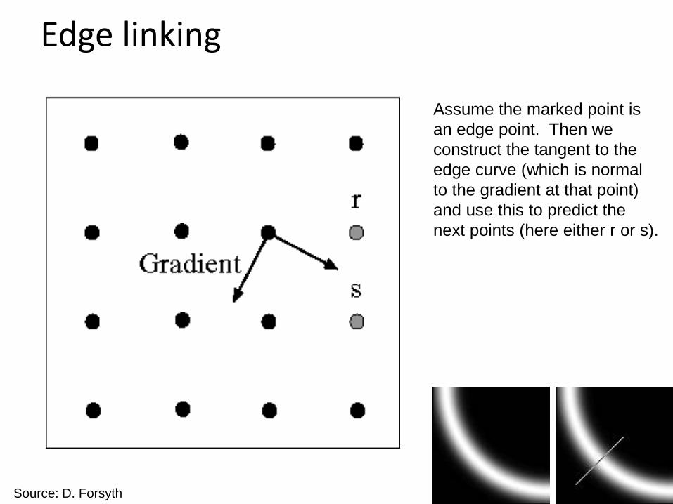
Assume the marked point is an edge point. Then we construct the tangent to the edge curve (which is normal to the gradient at that point) and use this to predict the next points (here either r or s).
Edge linking
Source: D. Forsyth
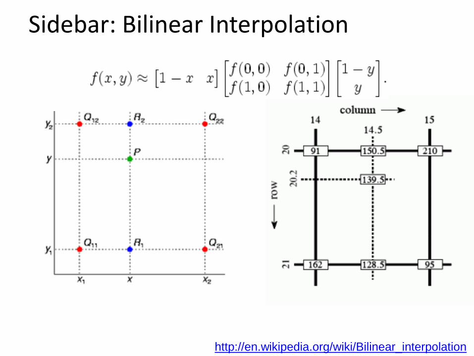
Sidebar: Bilinear Interpolation
http://en.wikipedia.org/wiki/Bilinear_interpolation
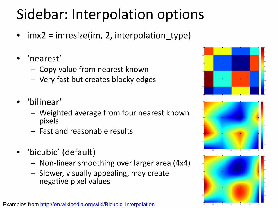
Sidebar: Interpolation options • imx2 = imresize(im, 2, interpolation_type)
• ‘nearest’
– Copy value from nearest known – Very fast but creates blocky edges
• ‘bilinear’
– Weighted average from four nearest known pixels
– Fast and reasonable results
• ‘bicubic’ (default) – Non-linear smoothing over larger area (4x4) – Slower, visually appealing, may create
negative pixel values
Examples from http://en.wikipedia.org/wiki/Bicubic_interpolation
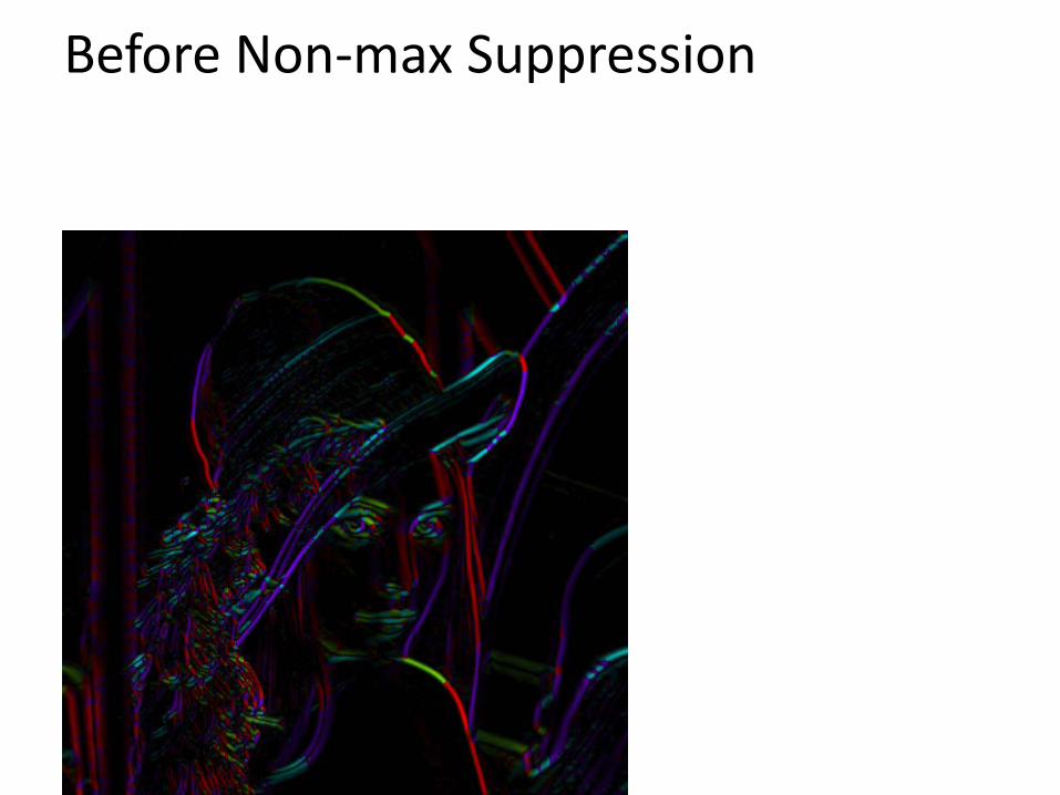
Before Non-max Suppression

After non-max suppression
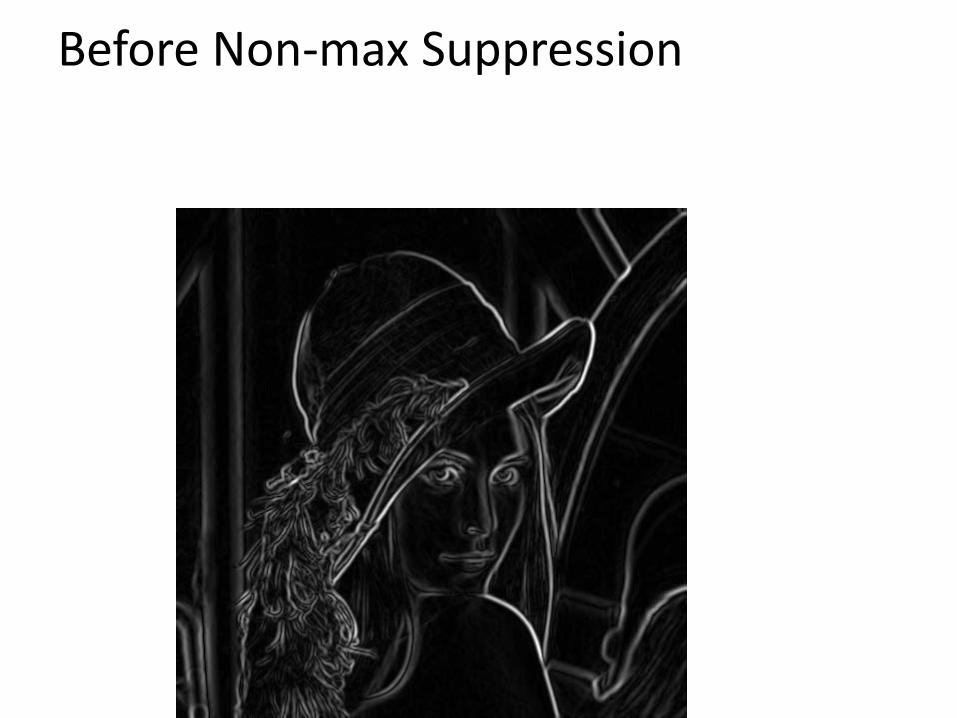
Before Non-max Suppression
After non-max suppression
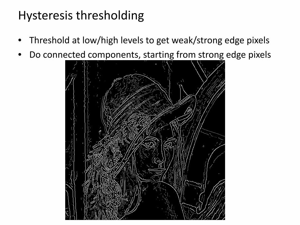
Hysteresis thresholding
• Threshold at low/high levels to get weak/strong edge pixels • Do connected components, starting from strong edge pixels
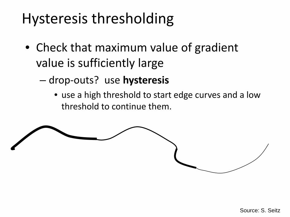
Hysteresis thresholding
• Check that maximum value of gradient value is sufficiently large – drop-outs? use hysteresis
• use a high threshold to start edge curves and a low threshold to continue them.
Source: S. Seitz
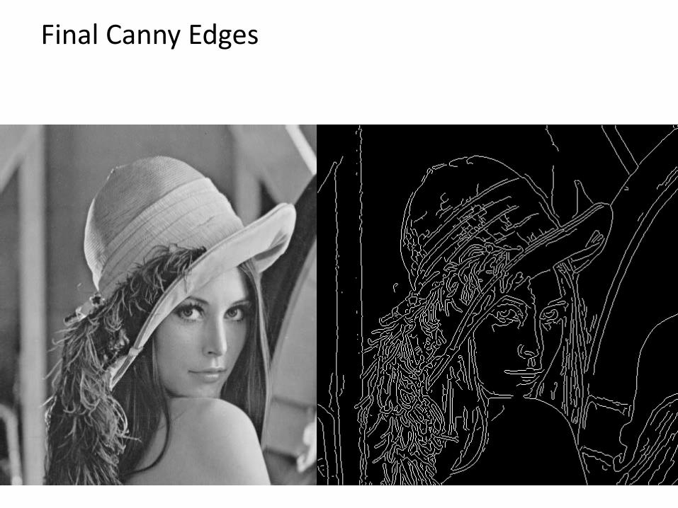
Final Canny Edges
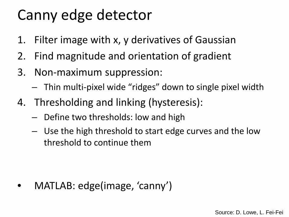
Canny edge detector 1. Filter image with x, y derivatives of Gaussian 2. Find magnitude and orientation of gradient 3. Non-maximum suppression:
– Thin multi-pixel wide “ridges” down to single pixel width
4. Thresholding and linking (hysteresis): – Define two thresholds: low and high – Use the high threshold to start edge curves and the low
threshold to continue them
• MATLAB: edge(image, ‘canny’)
Source: D. Lowe, L. Fei-Fei
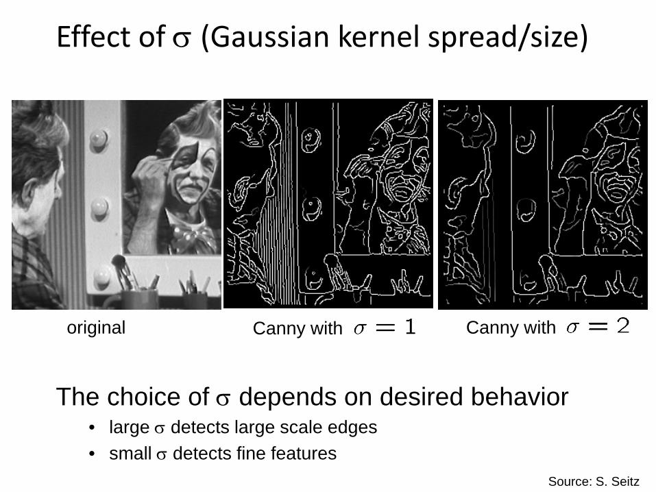
Effect of σ (Gaussian kernel spread/size)
Canny with Canny with original
The choice of σ depends on desired behavior • large σ detects large scale edges • small σ detects fine features
Source: S. Seitz