feynman diagrams and interaction rules of wave‐wave

G VOLUME 4 FEBRUARY 1966 NUMBER 1

Feynman Diagrams and Interaction Rules of Wave-Wave Scattering Processes

K. HASSELMANN

Institute of Geophysics and Planetary Physics, University o[ Cali[ornia, San Diego

Institute o[ Naval Architecture, University o[ Hamburg

Abstract. The energy transfer due to weak nonlinear interactions in random wave fields is reinterpreted in terms of a hypothetical ensemble of interacting particles, antiparticles, and virtual particles. In the particle picture, the interactions can be conveniently described by Feynman diagrams, which may be regarded either as branch diagrams of the perturbation expansion or as collision diagrams. The derivation of the transfer expressions can then be reduced to a few general rules for the construction of the diagrams and the associated collision cross sections. The representation follows closely the standard treatment of nonlinear lattice vibrations, but the particle picture differs from the usual phonon interpretation of lattice waves. It has the unreMistie property that the energies and number densities of antiparticles are negative. This is offset by simpler interaction rules and a closer correspondence between the perturbation graphs and collision diagrams. The method is illustrated for scattering processes in the oceanic wave guide involving surface and internal gravity waves, horizontal currents (turbulence), seismic waves, and bottom irregularities.

INTRODUCTION

The energy transfer due to weak nonlinear interactions between wave components can be an important factor in the radiation balance of a number of slowly varying geophysical wave fields. Recent investigations have led to a clearer un- derstanding of several of these scattering processes.

Nonlinear interactions between surface gravity waves have been studied by Phillips [1960], Hasselmann [1962; 1963a, b], Longuet-Higgins [1062], Benney [1962], Bretherton [1064], among others. Computations of the energy transfer for a random wave field were found to be in qualitative agreement with the observed decay of ocean swell [Snodgrass et al., 1965].

2 K. HASSELMANN

Scattering from gravity waves into elastic waves is one of the principal sources of microseisms. The conversion can occur either through direct nonlinear interactions between gravity waves [Longuet-Higgins, 1950] or through the interaction of gravity waves with an inhomogeneous ocean bottom [Wiechert, 1904]. Both processes have been quantitatively confirmed by measurements by Haubrich et al. [1963] [Hasselmann, 1963c].

The generation of long gravity waves with periods in •he minute range ('surf bea•' [Munk, 1949; Tucker, 1950]) may be a•tributed to a nonlinear gravity wave interaction plus a bottom interaction [Longuet-Higgins and Stewart, 1962; Hasselmann et al., 1963; Gallagher, 1965].

Sca•ering between surface and in•ernal gravity waves has been investigated by Ball [1964], Thorpe [1966], and Kenyon [1966]. Kenyon has computed •ransfer ra•es for both gravity wave and Rossby wave interactions.

Nonlinear interactions between surface gravity waves and quasi-s•eady cur- ren•s or •urbulence have been s•udied by Longuet-Higgins and Stewart [1961] and Phillips [1959].

Sca•ering processes very similar •o •hese geophysical examples have also been considered in o•her fields.

In a fundamental paper on •he hea• conduction in solids, Peierls [1929] investigated •he •ransfer effects due •o secular interactions between random lattice vibrations. Nonlinear interactions between ligh• waves and lattice vibrations, firs• investigated in •he classic papers of Brillouin [1922] and Raman [1928], have la•ely received renewed interest •hrough •he advances in laser technology. Stur- rock [1957], Litvak [1960], and o•hers have considered plasma wave interactions. The scattering formalism of quantum field theory may also b.e regarded as a generalized theory of nonlinear wave fields.

In the present paper, we apply some of the concepts developed in these fields to geophysical scattering problems. By using normal mode coordinates, the scattering theory is first presented in a Hamilt.onian form analogous to the usual treatment of lattice vibrations. Because of the analogy to quantum field theory, the transfer expressions can then be reinterpreted in terms of collision processes between hypothetical 'particles,' 'antiparticles,' and 'virtual particles.' This leads to a convenient description of the scattering processes in terms of Feynman diagrams, which may be interpreted either as perturbation graphs or as collision diagrams. By relating the formal perturbation expansion to the physical energy and momentum transfer rates, the diagrams enable the transfer expressions for all scattering processes t.o be reduced to a few general interaction rules.

The present particle picture differs from the usual phonon interpretation of lattice vibrations. In solid-state theory, the concept of a phonon is obtained by regarding the classical field as the limit of a quantized field. Our interpretation is analogous to Dirac's concept of positive-energy particles and negative-energy antiparticles (or positive-energy 'holes') introduced prior to the method of second quantization. This leads to simpler interaction rules and a closer correspondence between perturbation and collision diagrams. The interpretation yields negative number densities for antiparticles, but this is immaterial in the present context, since the particle picture is used only as an abstract description of the

WAVE-WAVE SCATTERING PROCESSES 3

effects of wave interactions. (The interpretation corresponds closely to the particle picture associated with the Klein-Gordon equation in ordinary quantum theory. I• is well known that the negative number densities caused SchrSdinger to abandon the relativistic Klein-Gordon equation in favor of the nonrelativistic equation which came to be known by his name.)

The method is illustrated for the case of scattering between surface gravity waves, internal waves, seismic waves, horizontal flows (turbulence), and physical inhomogeneities in the oceanic wave guide. Coupling coefficients for some of the processes not given previously in the literature are derived in the appendix.

1. WAVE INTERACTIONS

Equations o[ motion. Consider a eon[inuous, conservative sys[em which is homogeneous with respect to either two or three of the space coordinates x•, x2, xa. To first order, let the system be described by linear equations of motion with normal mode solutions of the form

or •(xs) exp [i(k.x 4- •t)] k: (k•, k2) x: (x•, x2) (1.1) • exp[i(k.xq-o•t)] k = (k•,k•,ks) x = (x•,x,•,xs), r = 1,2, ...

The dimensionality of x and k is irrelevant for the following. We assume that the set of eigenfunctions •ke is complete in the sense that

the amplitudes q• of the eigenfuncfions may be used as generalized coordinates to describe the state of the linear system. We assume further that the real, nonlinear system can be described by the same set of coordinates q• in a suitably extended representation.

Let the evolution of the real system be described by a Lagrangian L(q•, •). Introducing the generalized momenta p• = •L/• and the Hamil•onian

H =

we may write the equations of motion in the Hamiltonian form

• : 3H/3p• •5• = - 3H/3q• (1.2)

For an infinite system, k is a continuous variable. We shall regard k as discrete by the usual device of considering only periodic fields. In the final expressions the continuous case is recovered by letting the period approach infinity. The functions L and H are normalized by dividing by the volume of the periodic cell.

The linear system is described by a quadratic Lagrangian L2. For a homogeneous system, L• is independent of x and therefore contains only products of terms with equal and opposite wave numbers. For normal mode solutions of the form (1.1), the Lagrangian is then

L2 = Ck •q• • 2 q•:qkk ,

We assume the • to be normalized such tha• the constants C• = 1.

4 K. HASSELMANN

wi•h

The corresponding Hamiltonian is

= kw• q• .3)

' a[ = (a2•)* (1.9)

We assume now that •he Hamiltonian of the real system can be expanded in a Taylor series of the form

H H•+ y]n ............ = ••.a},•a•a•. + ... (1.10)

where in suitable units •he coupling coefficients are 0(1), and the field components a• are 0(X•), with X• << 1. We shall consider only lowest-order effects with respect

The reality condition is

Since H• is real, the components q• and p• satisfy the relations

q[• = (qSk)* p[• =

The linear solution is

•q• = A• exp (iw•t) q- B[ exp (-iw•t) (1.4) •pS}, = iw[A[ exp (iw•t) - iw•B• exp (-iw•t)

where A• and B• are determined by the initial conditions. Equation 1.4 represents a superposition of waves traveling in positive and

negative directions relative to k. It is convenient to introduce the transformation [cf. Peierls, 1929]

1

a[• - N//• (pSk - iw• q;) (1.5a) 1

a• • - •/• (pS• q- iw•q•) O' = 1, 2, ...) (1.5b) which in the linear case separates components traveling in opposite directions,

•a[ = a• exp (-iw[•t) •a• • = (aS•)* exp (•w},t) a• = constant (1.6)

Note that equation 1.5b defines a• for negative as well as positive r.

The equations of motion transform to

d,• = --iw• OH/Oa2• (r = 4-1, +2,...) (1.7)

where for negative r the frequencies are defined by w_-• = -w•. The Hamiltonian of the linear system becomes

•_• (1.8) k

v--+l,+2, ..o

WAVE.WAVE SCATTERING PROCESSES 5

•o •he parameters L bu• make no assumptions abou• •he relative magnitudes of k• for differen• •.

The coupling eoe•eien•s may be assumed symmetrical in •he index pairs (•). Because of •he homogenei•y and reality conditions we further have

D•k2":[[. = 0 for k• + ks + ... + kn • 0 (1.11)

Dk•k, 'kn -- '- '

The equations of mo%ion 1.7 lake %he form

= Dk•k,-kak•ak, + "' (1 13) ak -- •kak -- 3•wk ß

with initial conditions

a;(0) = a• (1.14)

Perturbation expansion, interaction diaqrams. We seek a solution to equation 1.13 in the form of a perturbation series

a• = •a• + 2a• + .-- (1.15) where

a • = o(x;)

The first-order solution is given by (1.6). It satisfies the initial condition rigorously. Higher-order solutions are obtained by successively substituting known lower-order solutions in the right-hand side of (1.13) and integrating,

p ß p plpa-p •ak(t) dr' exp [--i•[(t t')]{ 3• • Dk•k•_k •ak,(t') • • (t') • -- -- ak•

..... (p d- 1)i,o[ YI,Y2,

k• k2,.,,,k• n• + ß ß ß +rip =n

..... (n + vl,v•,

k• ks,''',kn

yl,

kx ka •1 +•2 --•

Yl ß ß 'yp-y rl /,) rp

Vx.oovn•v Vl ! o Vn (1.16)

is represented by p arrows (the components •a•} ... n,a•;) entering a vertex and a single arrow (the component A,a•) pointing away from the vertex. It follows from condition 1.11 that the vector sum of components minus anticomponents

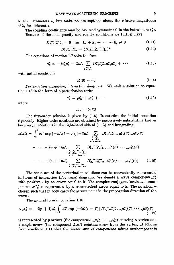
The structure of the perturbation solutions can be conveniently represented in terms of interaction (Feynman) diagrams. We denote a wave component with positive • by an arrow equal to k. The complex conjugate 'antiwave' component .a_-• is represented by a cross-stroked arrow equal to k. The notation is chosen such that in both cases the arrows point in the propagation direction of the waves.

The general term in equation 1.16,

A •ak = --i(p d- 1),o; dr' exp [-ioo[(t- t')] n•' .... -• • , • •,•,•...•,•_•, •a•,•(t) ... (1.17)

O K. HASSELMANN

entering a vertex is equal to the component (or minus the anticomponent) leaving the vertex.

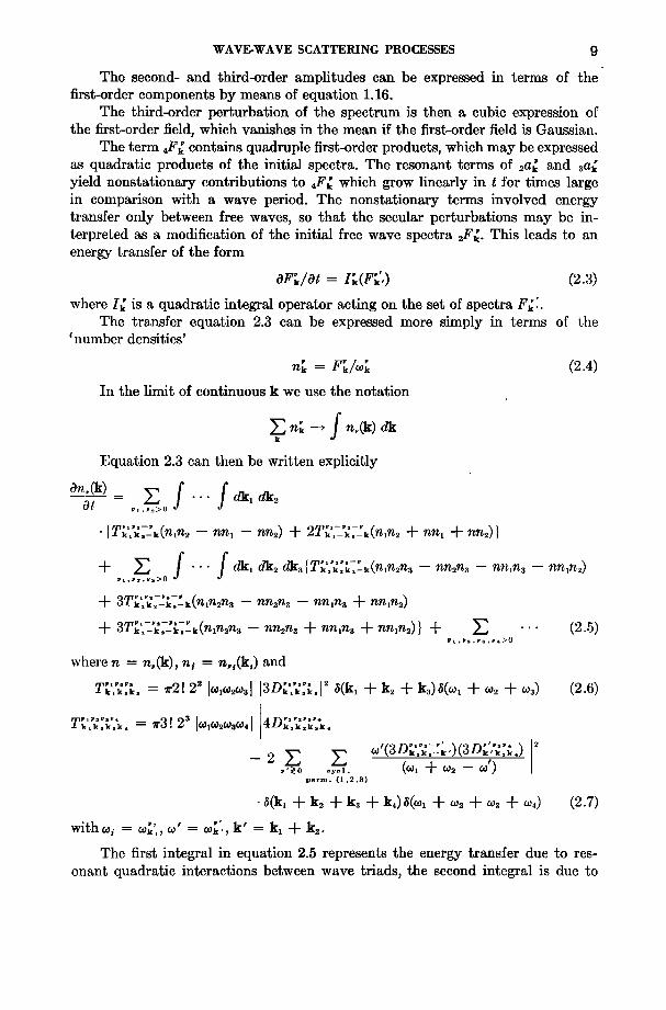
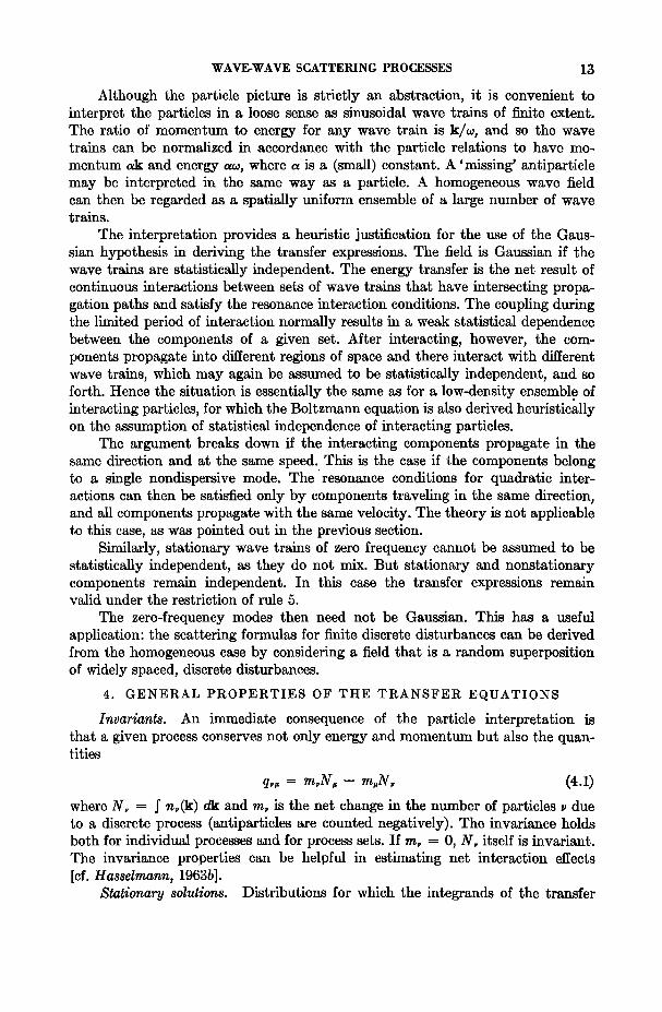
By successively representing components entering a vertex as interactions of lower-order components we obtain a cascade diagram with n first-order inputs and one nth-order output. The nth-order perturbation term is then the sum over all possible cascades with n first-order inputs (Figure 1).

We shall distinguish between 'virtual' and 'free' components of a cascade. Any pth-order component within a diagram is the product of a subcascade with p first-order inputs. If the frequency sum of the first-order input components is equal to the eigenfrequency of the resultant pth-order component, we shall refer to the component as 'free.' If it is not, we shall refer to the component as 'virtual.' Free components represent nonstationary resonant perturbations that may be interpreted as secular variations of the linear normal modes. Virtual components are forced, stationary waves that enter in the scattering calculations only as intermediate terms. In the lowest-order scattering theory we shall be concerned only with diagrams in which the final product is a free component and all internal components are virtual.

The resonance mechanism. Consider the second-order perturbation solu-

(o) (b) Fig. 1. Interaction diagrams for (a) second-order and (b) third-order perturbations. Anti- wave co.mponents are represented by crossed arrows, virtual waves by broken arrows. Further third-order interactions can be obtained by replacing wave components by antiwave com-

ponents.


tion, obtained by explicit integration of equation 1.16,

v v ß vl v• v 2ak = 3Wk • •k•_ka-_k ak•__ak• [exp [--t(wk• -+- Wk•)t] -- exp (--iwkt)] (1.18) Vl v• v

k•,k•

(a• = a• (0), equation 1.4). The terms in the sum represent stationary oscillations except for values of

k• and ks for which the denominator (w•} q- w•; - w•) vanishes. In this case we obtain resonant oscillations that grow linearly in time. The resonant terms have the same frequencies as normal modes and may thus be interpreted as a continuous, slow variation of the first-order normal mode field. If we include equation 1.11, the resonant conditions may be written

k• +k•-k = 0 wk• + v,• _ v = • wk• wk 0 (1.19)

It follows from the symmetry of the resonance conditions that, if a• is excited by a resonant interaction between a• and a•, the component a__-• (= (a•)*) is

•2 - .... by • a_-•. The three components excited by ak., a_k and the component a_k. ak•, form a mutually interacting triad.

Similarly, the expression for the third-order perturbation amplitude contains resonant terms representing interactions between coupled quadruplets, and so on. Generally, the nth-order resonance conditions may be written

kl-]- ... -]-k•-k•+l ..... k•+•-k= 0 .20)

vp vp+l vp+q v

(p + q = n, v• >0).

The resonant interactions produce a slow, continuous redistribution of the •node energies. I[ is inconvenien[ to analyze the finite changes arising in this manner in terms of a perturbation expansion with respect to the initial values of the field. This would require a cmnplete expansion [o all orders. The usual proce- dure is [o derive from the perturbation expansion an equation for the rate of change of the field a[ any given time, from which the finite secular change can be obtained by integration. This is feasible only in the limiting cases of a small number of discrete modes or a large s•a[is[ical ensemble.

For a finite number of modes the expressions for the resonant: perturbation terms may be simply rewritten as slow rates of change of •he mode amplitudes [ef. Benney, 1962; Ball, 1964; Bretherton, 1964; McGoldrick, 1965]. For a system of three modes the resulting nonlinear equations can be integrated explicitly in terms of elliptic functions.

In the case of a statistical ensemble the perturbation equations yield [ransfer expressions for t. he rate of change of the energy spectra [ef. Peierls, 1929, 1955; Prigogine, 1962; Hasselmann, 1962; Lityak, 1960]. For geophysical applications the statistical model is normally the more relevant. We shall be concerned here only with this case.

2. THE ENERGY TRANSFER

Consider the effect of weak nonlinear interactions in a statistical, homogeneous wave field.

8 K. HASSELMANN

For linear fields it can be shown that under very general conditions (smooth initial cumulants) the field tends asymptotically to a stationary, Gaussian state [Hasselmann, 1966]. This is valid in the coarse-grained sense that for finite spectral resolution the field cannot be distinguished asymptotically from a stationary, Gaussian field. Geophysical wave fields can be determined statistically (and in fact meaningfully defined) only with respect to a finite resolution. They may therefore always be regarded as stationary and Gaussian in the linear approximation.

A Gaussian field is determined by its second-order mean moments. In the case of the linear field (1.6) the only second-order mean products that are invariant under time and space translations are

where

(a•(t)a2•:(t q- •)) = 2F• exp (i•)

F• : «(a[,(t)a_-•:(t))= constant

The angle brackets denote ensemble mean values. The linear field is thus determined by the set of energy spectra F•. We shall

regard equation 2.1 as definition of F• for both positive and negative •, so that F_-• = F•. The mean energy of the field is then

k ,•,•o

The total energy density of the normal mode • (• > 0) is 2F•. In the nonlinear case, the spectra no longer remain constant because of the

energy transfer produced by the resonant interactions. For a field that is initially stationary and Gaussian, the initial rate of change of the spectra is a function of the spectra only, since the spectra completely specify the initial field. We shall assume that the resulting transfer expressions are in fact valid for all time. The evolution of the field is then statistically closed at the level of the energy spectra. The assumption implies that the resonant interactions produce a continuous redistribution of the energy but leave the statistical structure of the field essentially unchanged. It is not immediately apparent that this is mathematically consistent. A proof based on the derivation of the general term in the expansion of the master equation has been given by Prigogine [1962]. The self-consistency • fho (•-•ussian (random phase) hypothesis can be readily understood on physical grounds, as will be discussed later.

To determine the effect of the nonlinear coupling on the energy spectra we expand F• in a perturbation series

where

F• = 2F• •-3Fk •- -'-

F • i • -• 2 k -- •(lak la_k)= constant

(2.2)

4F;: = «{(,a; aa--;} q- (aa•: aa-•:} q- (aa; ß

ß


The second- and •hird-order amplitudes can be expressed in •erms of •he first-order components by means of equation 1.16.

The third-order perturbation of the spectrum is then a cubic expression of the first-order field, which vanishes in the mean if the first-order field is Gaussian.

The term •F• contains quadruple first-order products, which may be expressed as quadratic products of the initial spectra. The resonant terms of •.a• and •a• yield nonstationary contributions to •F• which grow linearly in t for times large in comparison with a wave period. The nonstationary terms involved energy transfer only between free waves, so that the secular perturbations may be in-

F • This leads to an terpreted as a modification of the initial free wave spectra a •. energy transfer of the form

OF•/Ot = I;(F•',) (2.3)

where I• is a quadratic integral operator acting on the set of spectra F•'. The transfer equation 2.3 can be expressed more simply in terms of the

' number densities'

n; = F•/• (2.4)

In the limit of continuous k we use the notation

•n•fn•(k)& k

Equation 2.3 can then be written explicitly

Z f ' {T•,•k(nln2 -- nn• -- nn2) + 2T•'l•,•k(nln2 + nn• + nn2)}

ß ß ß • • • • •_ • (n•nan• -- nnana -- nn•na -- nn•na) •l , 2 , 3 >0

+ 3Tk•_•_k•_kkn•na • -- nnan•. + nn•na + nn•na)} + • .. (2.5)

where n = n•(k), n• = n•,(k•) and

v, -'- (.Ok,

(2.6)

(2.7)

with w i = w•, w

The firs[ in[egral in equalion 2.5 represen[s [he energy [ransfer due to res- onan[ quadra[ie in[eraetions be[ween wave [riads, the second in[egral is due [o

10 K. HASSELMANN

cubic interactions between wave quadruplets, and so on. The resonance conditions find their expression in the $ functions in equations 2.6 and 2.7.

The cubic interactions could be neglected as compared with the quadratic interactions if all mode energies and coupling coefficients were of the same order of magnitude. In practice, the energies and coupling coefficients can vary by many orders of magnitude from one mode to another, so that the order of an interaction is not a reliable indication of the interaction rate. The third-order energy transfer between gravity waves, for example, is considerably larger than the second-order energy transfer from gravity waves to seismic waves.

The expression for the third-order transfer coefficient

k•k2k•k•

is valid only for mode combinations in which no quadratic resonant interactions occur between the modes v•, v2, and •3. The quadratic resonances produce non- integrahie singularities in the right-hand side of equation 2.6. It can be shown that in this case the quadratic interactions, which are already included in the first integral in (2.5), are always large as compared with the cubic interaction, regard- less of the relative intensities of the modes. A similar situation holds for the

fourth- and higher-order interactions. To lowest order, the sums in the right-hand side of equation 2.5 may therefore be restricted to the irr½o•c•bl½ mode combinations that contain no lower-order resonant subsets.

The integrals in equation 2.5 also diverge for interactions involving only components of a single, nondispersive mode. In this case the volume of the resonant subspaces defined by the $ functions becomes infinite. The theory is not applicable to these interactions. It can be shown that, if the field is initially Gaussian, the quadratic interactions produce a spectral perturbation that grows initially as t 3/2 instead of as L The physical reason for the breakdown of the theory in this case will be discussed later. The theory remains valid for interactions involving different nondispersive modes or combinations of dispersive and nondispersive modes.

The transfer expressions are also valid--under certain restrictions mentioned below--for interactions including degenerate, non-Gaussian modes of zero frequency. This is useful, for example, for scattering processes involving physical inhomogeneities or turbulence.

3. INTERACTION RULES

Equation 2.5 has the general form of a Boltzmann integral for interacting particles of momentum k and energy w, where n•(k) corresponds to the number density in x-k phase space of particles of type • and T is proportional to the differential scattering cross section. The resonant interaction conditions correspond to the conservation equations for momentum and energy.

The form of the individual interaction terms is not consistent, however, with the classical picture of an ensemble of positive-energy particles in which the probability of a collision is governed by the number densities of the approaching particles. The discrepancies can be removed either by assuming that the interaction


rate is dependent on the number densities of particles both before and after an interaction or by introducing negative-energy particles.

In the first approach, the transfer expression 2.5 is derived from the scattering formulas of quantum field theory by regarding the fields as the classical limit of quantized fields [cf. Peievls, 1955]. As in quantum theory, the transition probabilities are then dependent on the number densities of particles both before and after a collision. The energy of the particles is positive. This is clearly the only accept- able particle picture for systems in which quantum effects can be significant, such as in solid-state lattices.

For our purposes, we may ignore the implications of quantum theory and choose the particle picture that has the simplest interaction rules. This is obtained by introducing negative-energy antiparticles. We can then retain the classical expression for the collision probabilities. The interpretation also leads to a closer correspondence between the perturbation diagrams and the particle collision processes.

The transfer expression 2.5 may be regarded as the Boltzmann equation of a particle ensemble with the following properties'

1. The system consists of particles v of momentum k and energy •, and antiparticles -v (or •) with negative momentum -k and energy -•. The number density of particles and antiparticles is n• (k), and n_• ( - k) = -n• (k) (equation 2.4). Negative energies and number densities can be avoided by interpreting antiparticles in the Dirac sense as 'holes' in a 'sea' of negative-energy particles. For our purpose this is not necessary. The energy spectrum for both particles and antiparticles is the same, F•(k) = •n•(k).

2. Particles and antiparticles can be annihilated and created by collision processes. The interactions conserve energy and momentum. The processes either terminate in a single outgoing particle or begin with a single incoming antiparticle. The second processes may be regarded as the 'antiprocesses' of the first. We need consider only processes that terminate in a single particle; the 'antiprocesses' can be automatically taken care of by the rule that the creation or annihilation of an antiparticle is accompanied by the annihilation or creation of a particle (and vice versa). We need then keep track only of the number of particles n•(k); the number of antiparticles is always -n•(k).

3. The differential interaction rate of the process rl, r2, '" , r•, •+1, ''' , •,• --+ r, in which p particles and q antiparticles are annihilated and a particle v is created, is

Yl, '",•p,-•p+l, k •, ß ß ß, k•,--k• +•, ß ß ß,--k• +q,--k

ß l•(k•) ... •,(k•)•_•+•(-k•+•) ... •_•+•(-k•+•) I dk• ... dkv+• dk (3.1)

The coe•cient T is given explicitly for the cases p q- q = 2, 3 by equations 2.6, 2.7. The general expression may be obtained from the interaction (Feynman) diagrams (Figure 1), which we now interpret as collision diagrams. (We refer to the interaction diagrams as Feynman diagrams because of the general analogy to the Feynman diagrams and interaction rules of quantum field theory. The details differ; for example, in our case there is no vertical time orientation [cf. $chweber, 1961].)

12 K. HASSELMANN

Each vertex of a diagram represents the annihilation of two or more particles or antiparticles and the creation of a new particle •' or antiparticle -•'. The energy w' and momentum k of the new particle are determined by the conservation laws. If w' and k' do not satisfy the energy-momentum (dispersion) relation w' = w•', we refer to the new component as a virtual particle (or virtual antiparticle). Virtual particles occur only as intermediate products within a diagram.

Each vertex is associated with a propagator. The propagator of the vertex representing the annihilation of l particles and m antiparticles and the creation of a particle (antiparticle) • •' is given by

w •'''•,--•,+•'''--•,+m;•' (3.2)

The last vertex is an exception. In this case the propagator is

P = (1 • m • 1) •'•""'-"•'"'-"•-' (:].3) •kx ß ß .k l--k l+x .... k l+m--k

The produc• of sll propsgs½ors of s disgrsm yields ½he disgrsm amplit•de A•. The general expression for ½he collision transfer coe•cien½ is ½hen

•,...•_•+...._•+•_• = •(p + q)l 2 •+• ]•, ...

ß IZ A. + ... + - .... - k)

ß + ... + - .... -

where the sum is t•ken over all diagrams with given initial •nd final components. Equation 3.4 is v•lid for irreducible processes in which •11 internM com-

ponents of • diagram •re virtual. Processes containing real internal components c•n be neglected as compared with the two lower-order processes obtained by splitting the interaction diagram •t the re•l component.

4. If we write the process •, ß ß ß , r•, p•+•, ß ß ß p•+• • • •n interaction equation

then •11 processes obtained by rewriting the equation with •n •rbitr•ry positive term on the right-hand side have the s•me transfer coe•cient (principle of detailed bMance). This is not an independent rule but follows from equation 3.4 and the symmetry of the coupling coe•cients.

We shall denote the process set associated with a given transfer coe•cient by the symmetrical symbol (•, r:, ... •, p•+•, .-- p•+•, p). (The terms in the transfer integrals (2.5) •re •rr•nged according to process sets.)

5. The transfer expressions •re v•lid for processes containing degenerate modes of zero frequency, with the following restrictions: (a) the processes involve not more th•n one zero-frequency component •nd (b) components belonging to d•erent zero-frequency modes are statistically orthogonal. Condition (b) can normally be satisfied by suitable choice of representation.

The •bove rules determine the form of the transfer integrals for •11 irreducible scattering processes. Apart from su••rizing the transfer expressions, the rules •re useful for estim•tMg net scattering effects from the energy and momentum bMance of discrete processes (section 6).


Although •he particle picture is s•ric•ly an abstraction, i• is convenien• •o in•erpre• •he particles in a loose sense as sinusoidal wave •rains of finite ex•en•. The ra•io of momentum •o energy for any wave •rain is k/•, and so •he wave •rains can be normalized in accordance wi•h •he particle relations •o have momentum •k and energy •, where • is a (small) constant. A 'missing' an•ipar•icle may be interpreted in •he same way as a particle. A homogeneous wave field can •hen be regarded as a spa•ially uniform ensemble of a large number of wave •rains.

The in•erpreCa•ion provides a heuristic jus6fica6on for •he use of •he Gaus- sian hypothesis in deriving •he •ransfer expressions. The field is Gaussian if •he wave •rains are s•a•is•ically independent. The energy •ransfer is •he ne• resul• of continuous interactions between sets of wave trains that have intersecting propagation paths and satisfy the resonance interaction conditions. The coupling during the limited period of interaction normally results in a weak statistical dependence between the components of a given set. After interacting, however, the components propagate into different regions of space and there interact with different wave trains, which may again be assumed to be statistically independent, and so forth. Hence the situation is essentially the same as for a low-density ensemble of

ß

interacting particles, for which the Boltzmann equation is also derived heuristically on the assumption of statistical independence of interacting particles.

The argument breaks down if the interacting components propagate in the same direction and at the same speed. This is the case if the components belong to a single nondispersive mode. The resonance conditions for quadratic interactions can then be satisfied only by components traveling in the same direction, and all components propagate with the same velocity. The theory is not applicable to this case, as was pointed out in the previous section.

Similarly, stationary wave trains of zero frequency cannot be assumed to be statistically independent, as they do not mix. But stationary and nonstationary components remain independent. In this case the transfer expressions remain valid under the restriction of rule 5.

The zero-frequency modes then need not be Gaussian. This has a useful application: the scattering formulas for finite discrete disturbances can be derived from the homogeneous case by considering a field that is a random superposition of widely spaced, discrete disturbances.

4. GENERAL PROPERTIES OF THE TRANSFER EQUATIONS

Invariants. An immediate consequence of the particle interpretation is that a given process conserves not only energy and momentum but also the quantities

q• = m•N•- m•N• (4.1)

where N• = f n•(k) dk and m• is the net change in the number of particles • due to a discrete process (antiparticles are counted negatively). The invariance holds both for individual processes and for process sets. If m• = 0, N• itself is invariant. The invariancc properties can be helpful in estimating net interaction effects [cf. Hasselmann, 1963b].

Stationary solutions. Distributions for which the intogrands of the transfer

14 K. HASSELMANN

integrals vanish identically remain constant. The distributions are of the general form

n•(k) = (aw q- b.k) -• (4.3)

where a and b are constants. The same constants apply for all modes. The stationary solutions (4.3) were first given by Peierls [1929] for the case

of three-component interactions in solid-state lattices. If the processes leave the net number of particles of each mode unchanged, the solution is of the more general form

n•: (ao• q- b.k q- c) -• (4.3')

(for example, four-component gravity wave interactions [Hasselmann, 1963a]). For the number density (4.3) to remain positive, all phase velocities must

remain greater than Ibl/a (assuming a > 0 and • = •(lkl)). Thus, if the phase velocity of any mode approaches zero (e.g., internal waves or surface gravity waves without capillary forces), the only feasible distributions are the equi-energy distributions n = (a•) -•. (In the case of solid-state lattices, b = 0 follows from the finite folding wave number of the periodic lattice [Peierls, 1929].)

Irre•ersibility. The distributions (4.3), or (4.3'), are the only stationary solutions of the transfer equations; all other distributions approach these ir- reversibly.

Consider the quantity

f n•(k) $H = -- • lnn[(k ) dk (4.4) o (k) is the distribution at time t = to. •H corresponds to an entropy differ- where n,

ence. The entropy yln n,& itself is infinite, as expected for a system with an infinite number of degrees of freedom.

The rate of change of •H is governed by equation 2.5. After suitable permu- tation of the integration variables we find

d ff { [•11] a dt •H = • ß ß ß dr 1 &a dka nlnana • .... ..... >o 3 •k•k • , , • a- • n2

q- • ''' dkl dk. dka dk•

aq, .... _•_•, 1 1 1 n2 ns

n3

4

For most dispersion relations the distribution (4.3) yields infinite energies at high frequencies. Hence the general trend of nonlinear scattering processes is to transfer energy toward higher frequencies.

Processes involving zero-frequency components z require more careful con- sideration, since the number density n,(k) is infinite. The distribution (4.3) re-

It follows that d/dt/•H > 0 unless n•(k) is of the form (4.3).

]2} I q- -" (4.5) n4


mains valid for the finite-frequency components •, provided that the process contains at least three nondegenerate components. For quadratic processes of the form (•z•2) the energy distributions approach equidistributions at any fixed frequency, but there is no energy transfer between different frequencies.

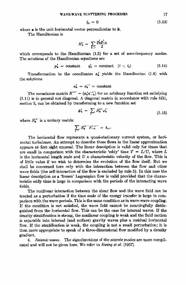
5. THE OCEANIC WAVE GUIDE

The Linear System

Consider a stratified fluid of constant depth h over a horizontally layered elastic medium. In the linear approximation the motions are composed of the following 'normal modes' [Eckardt, 1960; Ewing et al., 1957]:

1. Surface gravity waves, g. 2. Internal gravity waves, i. 3. Horizontal flows (turbulence), t. 4. Seismic waves, consisting of trapped 'organ pipe' modes s, trapped Love

modes a, leaking'organ pipe' modes s', and leaking Love modes a'. 5. Physical inhomogeneities, b.

Horizontal flows t and physical inhomogeneities b represent degenerate modes of zero frequency.

The dispersion curves are shown schematically in Figure 2. The phase velocities satisfy the order of magnitude relations

Ct, Cb << Ci • Cg • Ca, Cs, Ca,, Cs,

Let •.(r, rs) be the Lagrangian displacement of a particle (r, rs), where (r, rs) is the undisturbed equilibrium position of the particle. The eigenfunctions • and displacements are related as follows (eigenfunctions are normalized in accordance with equation 1.3):

1. Surface gravity waves.

• cosh k(x• q- h) (5.2) q•k -- (pg)•/%• cosh kh

o• = (gk tanh kh) •/" (5.3)

iki .k .r (5.4)

•3 • g ik or •ke (5.5)

where •' = O•/Ox3, p = fluid density, g = gravitational acceleration. The weak influence of density stratification and compressibility has been neglected.

2. Internal gravity waves. The eigenfunctions and frequencies are solutions of the eigenvalue equations

o?(p•')' q- p(N •-•)k• = 0 for -h <r3 <0 (5.6) gk•,•--•v' = 0 for rs = 0 (5.7)

v=0 for ra=-h (5.8)

16 K. HASSELMANN

b,t

Fig. 2. Schematic dispersion curves of oceanic wave guide modes. b _- 'bottom' wave, t -- horizontal flow (turbulence), i _-- internal gravity wave, g • surface gravity wave, s _-- trapped 'organ pipe' mode, s' m leaking organ pipe mode. Love modes are not shown [cf. Eckardt, 1960; Ewing

et al., 1957].

where N = (-g p'/p)•/" is the V/•is/d/• frequency. The normalization condition is

0 2 p•J,•--o -- p'• drs - •o (5.9) • g

The displacements are

ik• ß •i = • (•) 'e•k"

i •k .r

(• = •, 2)

(5.10)

Surface gravity waves are particular solutions of (5.6)-(5.8), but will not be classified as internal waves.

3. Horizontal flows. The eigenfunc•ions are members of a complete se• in -h < rs < O, which is normalized such that

•k,r3)•-k(r3) dr3 = •,•, (5.11) h

The displacements are

-•/2 • ,•.,• 2) (5.12) • = p .•,•e (•= 1,


(5.13)

where n is the unit horizontal vector perpendicular to k. The Hamiltonian is

t t

H' • PkP-k which corresponds to the Hamiltonian (1.3) for a set of zero-frequency modes. The solutions of •he Hamil•onian equations are

constant qL = constant (t- to) (5.14)

Transformation to the coordinates a• yields the Hamiltonian (1.8) with •he solutions

t --t

ak = ak = constant t t t --t •

The covariance matrix R t = (aka_k} for an arbitrary function set satisfying (5.11) is in general not diagonal. A diagonal matrix in accordance wi•h rule 5(b), section 3, can be obtained by •ransforming •o a new function set

,, (5.15)

where S•" is a unitary matrix tt'' t't''

•2] Sk S_k = •,,,

The horizontal flow represents a quasi-stationary current system, or horizontal turbulence. An attempt to describe these flows in the linear approximation appears at first sight unusual. The linear description is valid only for times tha• are small in comparison with the characteristic 'eddy' time T = L/U, where L is the horizontal length scale and U a characteristic velocity of the flow. This is of little value if we wish to determine the evolution of the flow itself. But we

shall be concerned here only with the interaction between the flow and other wave fields (the self-interaction of the flow is excluded by rule 5). In this case the linear description as a 'frozen' Lagrangian flow is valid provided that the characteristic eddy time is large in comparison with the periods of the interacting wave fields.

The nonlinear interaction between the shear flow and the wave field can be

treated as a perturbation if the time scale of the energy transfer is large in comparison with the wave periods. This is the same condition as in wave-wave coupling. If the condition is not satisfied, the wave field cannot be meaningfully distinguished from the horizontal flow. This can be the case for internal waves. If the density stratification is strong, the nonlinear coupling is weak and the fluid motion is separable into internal (and surface) gravity waves plus a residual horizontal flow. If the stratification is weak, the coupling is not a small perturbation; it is then more appropriate to speak of a three-dimensional flow modified by a density gradient.

4. Seismic waves. The eigenfunctions of the seismic modes are more compli- cated and will not be given here. We refer to Ewing et al. [1957].

18 K. ItASSELMANN

5. Physical inhomogeneities. The interpretation of physical inhomogeneities as normal modes of zero frequency will be deferred to the discussion of the nonlinear system.

The Nonlinear System

The normal mode solutions satisfy the equations of state only to first order. The total particle displacement in the linear approximation is

- qk• •k•k)e (5.16) k,y

where L: is a linear oberator acting on the •th eigenfunction. The equations of state can be satisfied to higher order by expanding the displacements in a perturbation series

where Q•2 •', ... are quadratic and higher-order operators. The Lagrangian L of the coupled system is obtained as a function of q•, • by evaluating the total potential and kinetic energy of the system for the displacement field (5.17). From L the Hamiltonian H(.-. a• -..) is obtained by the transformations described in section 1.

The evaluation of the coupling coefficients is rather tedious. Coupling coefficients for fourth-order gravity wave interactions and third-order interactions between gravity waves and seismic waves are given in Hasselmann [1962] and [1963c], respectively. Additional coupling coefficients for third-order interactions between surface gravity waves, internal gravity waves, horizontal flows, and bottom irregularities are given in the appendix.

Interactions due to physical inhomogeneities may be treated in the same way as nonlinear wave interactions. The equations of state consist of the stress-strain relations (for surface and internal gravity waves, these may be replaced by the incompressibility condition), to which we add the boundary conditions at the free surface and the fluid-solid interface. Physical inhomogeneities represent perturbations in these relations. For example, assume that the fluid-solid interface contains random perturbations •x3 relative to the mean interface x3 = -h. Let

$x• = •'• a•:e ,1•.: (5.18) k

where $x• is a homogeneous field with spectrum

F• • • • = •(al•a_l•) (5.19)

We introduce the negative index quantities b

a• b = ak F• b = F• .20)

in formal analogy with the relations for a zero-frequency mode. Then

<•x]) = • (F• + F• •) (5.21) k

The total energy H is a function of the normal coordinates a•, which are solutions of the equations of motion (1.7), and the external parameters a•, which


are prescribed constants. We can remove the distinction between internal and external variables by associating the external parameters with normal modes of

ß = = o, zero frequency. For co2 = 0 the equations of motion yield ak so that a• is indeed constant.

A few complications arise from the fact that for zero-frequency modes the positive and negative index components are identical. The HamiltonJan originally

b b

contains only positive index components ak; the representation in terms of ak b

and a• b is not unique. The components a• and a• b are, furthermore, not statistically independent, as in the case of finite-frequency modes. The correct transfer expressions are obtained by using only positive index terms in the Hamiltonian. In applying the interaction rules of section 3, it is then assumed that the same interaction coefficient applies for both positive and negative indices.

6. SCATTERING IN THE OCEANIC WAVE GUIDE

We shall denote wave components by letters g, i, t, ... corresponding to the mode indices introduced in the previous section. Antiwave components will be denoted by the symbols (g, •, •, --.). Different modes of the same mode type will be distinguished by indices, for example il, is, i3, .-- .

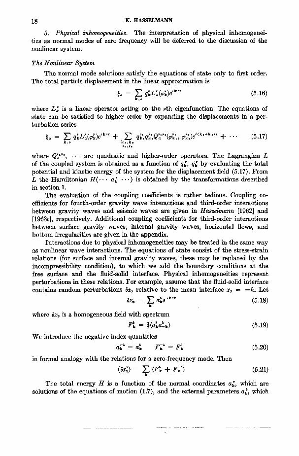
(gggg) interactions. The simplest scattering processes involving only surface waves are the quadratic processes (ggg). It has been shown by Phillips [1960] that these processes cannot satisfy the resonance conditions (1.19). The lowest- order interactions that conserve energy and momentum are the set (ggg•). The Feynman diagrams for these interactions are shown in Figure 3 (note that all processes belonging to (g•gg) are of the same form g•g --• g). Coupling coefficients and some computed transfer rates for typical ocean wave spectra are given in Hasselmann [1962, 1963b]. For most spectra there is a strong transfer from intermediate frequencies to higher frequencies and a weak transfer from intermediate

Fig. 3. Feynman diagrams of (ggg•) interactions.

20 K. HASSELMANN

frequencies to lower frequencies. The scattering computations are in good qualitative agreement with the observed 'red shift' of wave spectra shortly to lee of generating regions [Snodgrass et al., 1965].

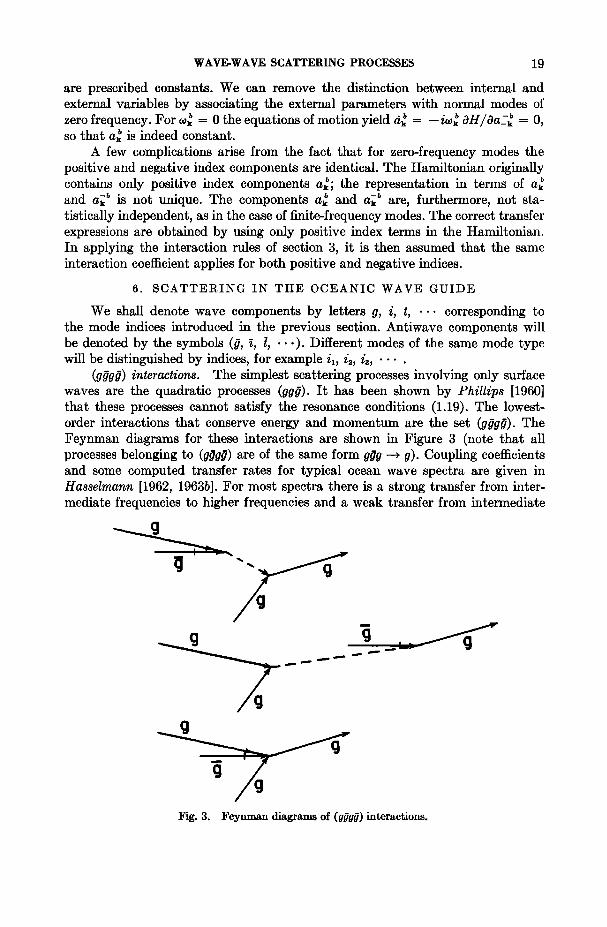
The 'sur[ beat' interaction g•b --• g. If one of the components g in the diagrams of Figure 3 is replaced by a bottom wave component b, we obtain the process g•b -• g. This is the 'surf beat' interaction, the generation of low-frequency gravity waves by difference interactions between gravity waves over a shoaling bottom [Munk, 1949; Tucker, 1950; Longuet-Higgins and Stewart, 1962]. The dominant interaction is given by the diagram in Figure 4. The quadratic interaction among

Fig. 4. The 'surf beat' interaction g•jb -• g.

g, •, and the virtual component g' has been verified experimentally by bispectral analysis methods [Hasselmann et al., 1963]. The complete process has been computed by Gallagher [1965], who found good agreement with observations by Snod- grass et al. [1965]. (Gallagher used as model a constant-slope bottom. For this case the theory needs to be modified, since the bottom variations cannot be regarded as perturbations relative to a bottom of constant depth.)

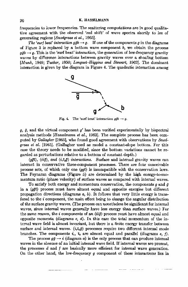
(g•), (ii•), and (i•2•) interactions. Surface and internal gravity waves can interact in conservative three-component processes. There are four conceivable process sets, of which only one (gg•) is incompatible with the conservation laws. The Feynamn diagrams (Figure 5) are determined by the high energy-to-momentum ratio (phase velocity) of surface waves as compared with internal waves.

To satisfy both energy and momentum conservation, the components g and • in a (g•) process must have almost equal and opposite energies but different propagation directions (diagrams a, b). It follows that very little energy is trans- fered to the i component, the main effect being to change the angular distribution of the surface gravity waves. (The process can nonetheless be significant for internal waves, since internal waves generally have less energy than surface waves.) For the same reason, the i components of an (ii•) process must have almost equal and opposite momenta (diagrams c, d). In this case the total momentum of the internal wave field is almost invariant, but there is a finite energy transfer between surface and internal waves. (ixk•) processes require two different internal mode branches. The components i•, • are almost equal and parallel (diagrams e, •).

The process g• -• i (diagram a) is the only process that can produce internal waves in the absence of an initial internal wave field. If internal waves are present, the processes d and [ are basically more efficient for internal wave generation. On the other hand, the low-frequency g component of these interactions lies in


_ i g

(a) (b (c)

....g

i i• 2

g g

(d) (e)

Fig. 5.

(f) Feynman diagrams of interactions between surface and

internal gravity waves.

• very low density region of the spectrum, so that the relative importance of the interactions is difficult to estimate.

Interactions between discrete surface waves and internal waves have been

studied by Ball [1964] and Thorpe [1966]. The statistical case is being investigated by Kenyon [1966].

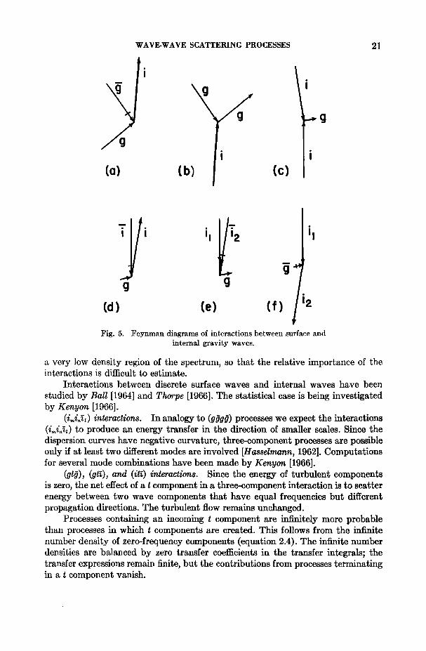
(imin•z) interactions. In analogy to (g•gO) processes we expect the interactions (imi,•Z) tO produce an energy transfer in the direction of smaller scales. Since the dispersion curves have negative curvature, three-component processes are possible only if at least two different modes are involved [Hasselmann, 1962]. Computations for several mode combinations have been made by Kenyon [1966].

(gt•), (gt•), and (it•) interactions. Since the energy of turbulent components is zero, the net effect of a t component in a three-component interaction is to scatter energy between two wave components that have equal frequencies but 'different propagation directions. The turbulent flow remains unchanged.

Processes containing an incoming t component are infinitely more probable than processes in which t components are created. This follows from the infinite number density of zero-frequency components (equation 2.4). The infinite number densities are balanced by zero transfer coefficients in the transfer integrals; the transfer expressions remain finite, but the contributions from processes terminating in a t component vanish.

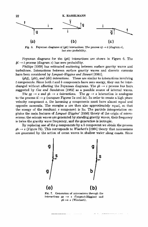
22 K. HASSELMANN

(a) Fig. 0.

(b) (c) Feynman diagrams of (gt•) interactions. The process i# -• t (diagram c),

has zero probability.

Feynman diagrams for the (gti) interactions are shown in Figure 6. The •i -• t process (diagram c) has zero probability.

Phillips [1959] has estimated scattering between surface gravity waves and turbulence. Interactions between surface gravity waves and discrete currents have been considered by Longuet-Higgins and Stewart [1961].

(gb•), (gb•), and (ibm) interactions. These are similar to interactions involving t components. Since both t and b components have zero energy, they can be inter- changed without affecting the Feynman diagrams. The gb --• i process has been suggested by Cox and Sandstrom [1962] as a possible source of internal waves.

The gg --• s and gb --• s interactions. The gg --• s interaction is analogous to the process ii --• g (compare Figures 7a and 5c). In order to create a high phase velocity component s, the incoming g components must have almost equal and opposite momenta. The energies o• are then also approximately equal, so that the energy of the resultant s component is 20•. The particle interpretation ex- plains the main features of Longuet-Higgins' [1950] theory of the origin of microseisms' the seismic waves are generated by standing gravity waves, their frequency is twice the gravity wave frequency, and the generation is isotropic.

By replacing one of •he g components by a b component we obtain the process gb --• s (Figure 7b). This corresponds to Wiechert's [1904] theory that microseisms are generated by the action of ocean waves in shallow water along coasts. Since

g

g

g

b

(a) (b) Fza. 7. Generation of microseisms through the interactions gg .--) s (Longuet-Itiggins) and

gb ---) s (Wiechert).

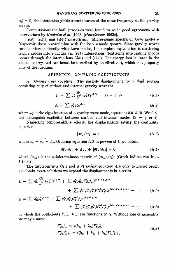
WAVE-WAVE SCATTERING PROCESSES

• = 0, •he interaction yields seismic waves of •he same frequency as •he gravity w•ves.

Computations for both processes were found to be in good agreement with observations by Haubrich et al. [1963] [Hasselmann 1963c].

(sb•), (sb•'), and (sb•') interactions. Microseismic spectra of Love modes frequently show a correlation with the locM s-mode spectrm Since gravity waves cannot interact directly with Love modes, the simplest explanation is scattering from s modes into a modes via (sb•) interactions. Scattering into leaking modes occurs through the •teractions (sb•') and (sb•'). The energy loss is linear in the s-mode energy and can hence be described by an effective Q which is a property only of the medium.

APPENDIX. COUPLING COEFFICIENTS

A. Gravity wave coupling. The particle displacement for a fluid motion consisting only of surface and in•ernal gravity waves is

• = Z q• •• (•) 'e•'• (• = 1, 2) (A.I) = q•e (A.2)

where • is the eigenfunction of a gravity wave mode, equations 5.6-5.10. We shall not distinguish explicitly between surface and internal modes (h = g or i).

Neglecting compressibility effects, the displacements satisfy the continuity equation

[Ox•/Or• = 1 (A.3)

where x• = r• + •. Ordering equation A.3 in powers of •, we obtain

where (A•,) is the subdeterminant matrix of (0•/0r,). (Greek indices run from 1 to3.)

The displacements (A.1 and A.2) satisfy equation A.4 only to lowest order. To obtain exact solutions we expand the displacements in a series

ik• ½eik.r = qk•qk•ik•k•e

qk•qk•qk•vik•k•k•e + ß ' ' (A.5)

•a = qk•ke + qk•qk,•k•k•e

+ • k• k2 ka •k•k2ka i(k•+k2+ka)'r

in which the coe•cients F:"., G'" are functions of r•. Without loss of generality we may assume

x•x• k •F

t' ikxk2k3 • 3

24 K. HASSELMANN

Substituting equations A.5 •nd A.6 in Equation A.4 we obtain the conditions

ß •, , • •x, • (•,)'(1 + k•k• ]

- •,(•,)"-,•- •,(•,)" (•.s) k• k•

* 3] k•kuk,

= (•k•) (•k•) • + •k•k•k•) • • •e . o• indiees

twX,X, / X, xtt (kl'ka q- •F •'• '• •(k, k• • k•'ks)

(• (•)' • - • •

_ (•;), • , • (•1.•)(•.•) - klk•

with the boundary conditions

and

(A .9)

(A.10)

•,•,•., = 0 for ra = -h (A.11)

Equations A.8, A.9, ... do not determine the coefficients F":, G'" uniquely. An arbitrary solution of the homogeneous equations may be superimposed at each order. However, the homogeneous solutions satNfy the linear continuity equation O•/Or• = 0 and may hence be included in the definition of the linear field. This is equiwlent to a nonlinear transformation

= •k,k,kqk,qk, + ''' (A.12)

to new coordinates q•. (The same applies to the generalization of expressions A.7. In this case the nonlinear transformation would involve shear flow components.) A nonlinear •ransformation of the form (A.12) yields new nonlinear coupling co- e•cients. It is readily verified, however, that the coupling coe•cients remain invariant for wave-number combinations •hat satisfy the resonance conditions. Hence •he scattering expressions are independent of •he choice of solution of equations A.8-A.11.

The kinetic energy of the field is

17 = fi drap .X

, k•+ku+ka=O X• ,X•


where

fh dra denotes the mean value of the integral

f: dr• h

with respect •o r. The form of the quadratic term follows from equations 5.6-5.8 and the normalization condition (5.9).

The potential energy is

U = g dr•p• h

= g q•q• dr•pG• • g q•q•q•. dr•pG•• . k•+ka=0 h kx+ka+ks=0 h

The quadratic term has the expected normal form (equations A.8, 5.6-5.9)

The cubic term is determined by equation A.9. For kx + k• + k• = 0 the expression simplifies,

• - • ks- k•ka + 1 -- Gkxk -- Fk•k .

petra.

The Lagrangian L = V - U is thus of the form

L = L• + • {A •' • •' •' ,•x,x• • .•, .• kx+ku+ka=0

with coupling coe•cients

'z•' k xk ak s 3 c . h perre.

- - o

h

F•?• and , ,•, are arbitrary solutions of equation A.8 and the boundary condition (A.10), for example

k•k' -- 2(k• + k=) (•k)'(•)' 1 -- -i'• ' + •k•t•k,½ 1 + kz ] •k, 1 + (A.18)

x•x, _ x x• x, , ,.x,x (A.19)

20 K. HASSELMANN

The cubic coupling coefficient of the Hamiltonian (1.10) is obtained by transforming to the coordinates a• x. We obtain

r•X•x•x•, i { A••' B•: •' B•' • ,-- 1 2ks •k,k,k, 6 •2 3 -- -- -- (A.20) •1•2•3 •1 •2

with • = •,, • = I•1, • • 0.

The coupling coe•cients can be determined by quadrature if the eigenfunctions are known. Expressions for specific models are given by Ball [1964], Thorpe [1966], and Kenyon [1966]. Coupling coe•cients and transfer rates for fourth-order (g•g•) interactions between surface gravity waves are given in Hassel- mann [1962].

B. Interactions between gravity waves and 'bottom' waves. Let the fluid bottom be x• = -h + •x•, where

•X 3 • b ik 'x = ake (5.18) k

The boundary condition for the fluid displacement at the bottom is

•x•(r) + •(r,-a + •x•(r)): •x•(r + •(r, -a + •x•(r))) (B.•)

Expanding (B.1) about r and r• = -h, we obtain

• + •xs•] O•xs 1 OaSxs • ..... 0 (B.2) - Ox• • 20x• Consider a linear flow that consists only of gravity waves, equations A.4, A.5.

To obtain a displacement field satisfying the exact continuity equation A.4 and the boundary condition (B.2) we expand as before

= • • (• + •a•)••e • E q• ••• (•) 'e•k + i E q•ak• 1• qk• qk•(kl• + kai)Fk•k•e

qk,q•,a•,(kli + k•i + k•i)F•k •e ak

+ ... (g.3)

q•e + • q• = •ak•k• •e

Substituting in (A.4) and (B.2), we find

•)'- (kl + •a: ,. • = 0 (B.5)

with the boundary condition

Xb ( kl Gk•k• -- (e•)' 1 +--•--] for ra = --h (B.6) and for kl • k2 • k3 • 0

eX•X•b M •Xab Xa Xxb • + (• ) } + co,rant (B.7) • ek•ka


The constant is determined by the boundary condition

- • for r• = -h (B.8)

We may again choose arbitrary solutions of (B.5) and (B.6), for example

= 0

In analogy to equations A.13-A.17, we obtain a Lagrangian Akxkab Xx ka b kxkab .ka b L L• + • {•• q•q•a• +B•• • : • • • qk•ak•

where

Ak,k2k3 -- arapg•k,k2k3 (B.9) h

0

Bk•k,k -- ß h

The corresponding coupling coefficient of the HamiltonJan (1.10) is •hen

fA*•*•* } •k•k ka(: •kakak •kak•k ) • • •1•2 xi where wi = wki, •i = [Xi , and X• • 0, as before.

The transformation from the variables q}, •} to the coordinates a}, a[ x yields a coupling coefficient D x•x•* k•k,k. which is defined only for positive b. To obtain the correct transfer rates from the interaction rules of section 3, equation B.11 must be taken to apply for both positive and negative b.

The total energy transfer due to (XbX) scat[ering processes may then be written in the form

OFx(k) f ,) &, at - x,>•o Kxx,(k, k') lFx,(k') - Fx(k)}a(w - w (B.12) where the kernel

Kxx, = 32•r 3wDX•'?•,x,_kl2 Fb(k") k" = k - k' (b > 0) (B,13)

C. Interactions between surface gravity waves and horizontal shear flows. I• is inconvenient •o investigate higher-order secular interactions between gravity waves and horizontal flows in a Lagrangian coordinate system, since the first- order Lagrangian amplitudes for •he horizontal flow appear formally as secular terms. We therefore use Eulerian coordinates. Later we shall construct a Hamil-

tonian •hat yields the secular •erms of •he Eulerian perturbation equation. (This is feasible, although the transformation from Lagrangian to Eulerian coordinates is noncanonical.) The analysis is thus again reduced •o the general theory outlined in sections 1-3.

28 K. HASSELMANN

and take p = constant. The equations of motion, continuity equation, and boundary conditions are then

Ou . Ou . I __

Ot + u• Ox• p Ox. g/i.a ( h < xa < O) (C.1) Ou. _ 0 (-h < x• < 0) (C.2)

o•. o•. ot u• + u• •x• = o (x• =

go = 0 (x• --' •')

u• =0 (x• = - h)

where g is the surface elevation. Expanding equations C.3 and C.4 about xa = O, we have

.3)

(c .4)

(c .5)

0•' Ou____• 0•' ot u• - Ox• •' + u• •x• + .... 0 (x• = o) (C .3')

.... o From (C.1) and (C.5) we obtain the subsidiary condition

(x• = 0) (C .4')

O•o/Oxa = -- g (xa = - h) (C.6)

The fluid motion may be represented as a superposition of an irrotational 'wave' motion u• and a residual rotational flow ur. We define u• as the irrotational flow satisfying the boundary conditions u•(0) - u(0), u•(-h) = 0. For a homogeneous field the boundary conditions determine u• uniquely except for an arbitrary additive solution u = (a•, a0, with a• = constant. We assume a i = O.

The general solutions of the linearized equations are:

(C .7)

(c.s)

(C .9)

(C.10)

where

wave motion

and

q• = A• exp (- i.,• t) + B• exp (i.,• t) (A•, B• constant)

(o.,• = (gk tanh kh) •/')

(C.11)

(C.12)


shear flow

u•

where p• and p• are constant, • and • are complete sets of functions in -h < xa < 0, and n is the unit horizontal vector perpendicular to k.

The functions • satisfy the boundary conditions •(0) = • (-h) = 0. They correspond to internal waves in the case of a stratified fluid. For simplicity we take p• = 0, so that •he rotational flow is purely horizontal. The functions • are •ssumed normalized in accordance with equation 5.11.

The time dependence of the variables q•, p•, and p• corresponds •o the solutions of the free HamiltonJan

H• = • • + 2 q• + 2 In the nonlinear case the expressions C.7-C.9 and C.13-C.15 for the velocity

field and the surface displacement remain valid, but the pressure field and hence the time dependence of the variables q•, p•, and p• are modified.

The pressure field may be expressed as the superposition of a hydrostatic field and two fields • and

where

and

Let

Then

• -- --pgx3 q- •)a + •b

2 •a = o (-a < x• <o)

a(o) =

O •)a/ OX3 (-- h) --- 0

V '• •b = -- p Ox • cqx• (-h < x3 < O)

= o

= o

•)(0) = • •k(t)e 'k'x k

p,, = •'• •k cosh k(xs q- h) k cosh kh ik ox

e

(C.17)

(C.18)

(C.19)

(c .20)

(C.21)

30 K. HASSELMANN

Similarly, if

k

02U -- POx,, Ox• = • Q•,[x•, t)e •"x

sinh [k(xs - x])] k dx• + cosh k(x, + h) Qk(x•)

cosh kh h

(C .22)

sinh kxg k dx• (C .23)

The rate of change of the coordinates q• and p• is determined by equation C.1 (with a = 3, x, = 0) and the boundary condition (C.3'). Eliminating g2 with the aid of equations C.4', C.17-C.23, we obtain

pSk = --(co•)'q• + • A go' ,p5 •,• • •, + .-. (C.24) k•+k,:-k

= ••,q•p_•. (C.25) k•+k•:-k

where we have written only the cross terms relevant for (gt•) interactions. The coefficients are

A• •, i(k.?) {co ' g(k•- 2k.kl) f: cosh • k(x, + h) - + cok co• h cosh kh axe} (c.26)

kk•k. = --i--7 (k.,•)•(O) (C.27) (.o k

Introducing the coordinates a• and a• • in accordance with the transformation (1.Sa), (1.Sb) and writing

1

(equation 1.5a for a zero-frequency mode), we obtain

(c.28)

i "•' (a• -- a•)a • -•,•,1•,, • •, (g > O)

¾2

(C.29)

For the scattering calculations only the resonant values of the coefficients A •' and •, ,_,•, are of interest. In the present case the resonant condition is co• = co• or, equivalently, k• = k. For these values the coefficients satisfy the symmetry relations

Aggt kk•k= -- -A aa' • -k•-kk• (c.3o)

Bg•' - "•' (C.31) kk•k• -- --L•-k•-kk•

It follows from (C.30) and (C.31) that the secular s3lutions of (C.28) and (C.29) are identical with the secular solutions of the equations

c• = --• OH/Oa_-• (g • O)

WAVE. WAVE SCATTERING PROCESSES 31

where

k•+ke+ka=O

with the symmetrical coefficient

Dgxg• t •'•tgxg2 • • kakak• -- •k•k•ka)

(C .32)

f K(k, k'){F•(k') - F•kk)} •(•0 - •0') dk' (C.34)

K = 32•r • z Ft(k") (C.35) t>o

(k" = k - k', > 0).

Computations of (C.34) for suitable horizontal flow models would be of interest, but they have not yet been made. Experimentally, (gt,•) interactions are difficult to distinguish from (g,•g,•) interactions, since both produce a beam broaden- ing of ocean swell [Snodgrass et al., 1965].

Acknowledgment. This work was supported in part by the National Science Foundation under grant GP2414.

REFERENCES

Ball, F. K., Energy transfer between external and internal gravity waves, J. Fluid Mech., 19(3), 465-478, 1964.

Benney, D. J., Nonlinear gravity wave interactions, J. Fluid Mech., 14(4), 577-584, 1962. Bretherton, F. B., Resonant interactions between waves, The case of discrete oscillations, J.

Fluid Mech., 20(3), 457-479, 1964. Brillouin, L., Diffusion de la lumi•re et des Rayons X par un corps transparent homog•ne,

Ann. Phys. (Paris), 17, 88-122, 1922. Cox, C., and H. Sandstrom, Coupling of internal and surface waves in water of variable depth,

J. Oceanog. Soc. Japan (20th anniversary vol.), 499-513, 1962. Eckardt, C., Hydrodynamics o/Oceans and Atmospheres, Pergamon Press, New York, 1960.

ing may then be written

OF•(k) __

ot

where

__ 21 - ]• g(kl'U3)(k•- 2,k•1*k2) • cosh 2 kl(X3 + h) t p .... 6 X/• (o•,) - h cosh k,h •k•(x•) dx• (C.33) (1,2)

(gl, g• • 0, • • 0).

The Euleri•n equations for gravity w•ve perturbations c•n hence be reduced to the general H•miltoni•n formalism of section 1.

The H•miltoni•n equations •lso •pply to the perturbations of the rotational flow. S•ce • = 0, equation 1.7 yields a• = 0. This •grees with the Eulerian perturbation •n•lysis, which yields • zero quadratic coupl•g coe•cient for the g• • t interaction. This follows from Helmholtz's theorem: nonlinear interactions between potential flow components c•n generate only potentiM flow perturbations.

In •nMogy with equation B.12, the total energy transfer due to (gt•) scatter-

32 K. HASSELMANN

Ewing, W. M., W. S. Jardetzky, and F. Press, Elastic Waves in Layered Media, McGraw-Hill Book Company, New York, 1957.

Gallagher, B. S., Generation of surf beat by a nonlinear mechanism, Ph.D. thesis, University of California, S•n Diego, 1965.

Hasselmann, K., On the nonlinear energy transfer in a gravity-wave spectrum, 1, General theory, J. Fluid Mech., 12(4), 481-500, 1962.

Hasselmann, K., On the nonlinear energy transfer in a gravity-wave spectrum, 2, Conservation theorems, wave-particle correspondence, irreversibility, J. Fluid Mech., 15, 273-281, 1963a.

I-Iasselmann, K., On the nonlinear energy transfer in a gravity-wave spectrum, 3, Computation of the energy flux and swell-sea interaction for a Neumann spectrum, J. Fluid Mech., 15, 383-398, 1963b.

Hasselmann, K., A statistical analysis of the generation of microseisms, Rev. Geophys., 1(2), 177-210, 1963c.

I-Iasselmann, K., On the Gaussian property of linear wave fields, in preparation, 1966. I-Iesselmann, K., W. It. Munk, and G. J. F. MacDonald, chapter 8, in Time Series Analysis,

edited by M. Rosenblatt, John Wiley & Sons, New York, 1963. I-Iaubrich, R. A., W. It. Munk, and F. E. Snodgrass, Comparative spectra of microseisms and

swell, Bull. Seismol. $oc. Am., 53, 27-37, 1963. Kenyon, K. E., Ph.D. thesis, University of California, San Diego, in preparation, 1966. Lityak, M. M., A transport equation for magnetohydrodynamic waves, AVCO-Everett Res.

Lab. Res. Rept. 92, 1960. Longuet-Higgins, M. S., A theory of the origin of microseisms, Phil. Trans. Roy. Soc. London,

A, 2•3, 1-35, 1950. Longuet-I-Iiggins, M. S., Resonant interactions between two trains of gravity waves, J. Fluid

Mech., 12(3), 321-332, 1962. Longuet-I-Iiggins, M. S., and R. W. Stewart, The changes in amplitude of short gravity waves

on steady nonuniform currents, J. Fluid Mech., 10, 529-549, 1961. Longuet-I-Iiggins, M. S., and R. W. Stewart, Radiation stress and mass transport in gravity

waves, with application to 'surf beats,' J. Fluid Mech., 13, 481-504, 1962. McGoldrick, L. F., Resonant interactions among capillary gravity waves, J. Fluid Mech., 21(2),

305-331, 1965. Munk, W. M., Surf beats, Trans. Am. Geophys. Union, 30(6), 849-954, 1949. Peierls, R., Zur kinetischen Theorie der Warmeleitungen in Kristallen, Ann. Phys., 3, 1055-

1101, 1929. Peierls, R. E., The Quantum Theory o• Solids, Clarendon Press, Oxford, 1955. Phillips, O. M., The scattering of gravity waves by turbulence, J. Fluid Mech., 5, 177-192, 1959. Phillips, O. M., On the dynamics of unsteady gravity waves of finite amplitude, 1, The ele-

mentary interactions, J. Fluid Mech., 9, 193-217, 1960. Prigogine, I., Non Equilibrium Statistical Mechanics, Interscience, New York, 1962. Raman, C. V., A new radiation, Indian J. Phys., 2, 387-398, 1928. Schweber, S.S., An Introduction to Relativistic Quantum Field Theory, Harper and Row

Publishers, New York, 1961. Shodgrass, F. E., G. W. Groves, I•. F. I-Iasse!mann, G. R. Miller, W. /-I. Munk, and W.

Powers, Propagation of ocean swell across the Pacific, Phil. Trans. Roy. Soc. London, A., in press, 1965.

Sturrock, P. A., Nonlinear effects in electron plasmas, Proc. Roy. Soc. London, A., 242, 277- 299, 1957.

Thorpe, S. A., submitted to J. Fluid Mech., 1966. Tucker, M. J., Surf beats: sea waves of I to 5 rain period, Proc. Roy. Soc. London, A, 202,

565, 1950. Wiechert, E., Getlands Beitr. Geophys., 2, 41-43, 1904.

(Manuscript received November 19, 1965.)

feynman diagrams and interaction rules of wave‐wave

Documents