fermi golden rule and open quantum systems
TRANSCRIPT
Fermi Golden Rule and open quantum systems
Jan Derezinski and Rafał Fruboes
Department of Mathematical Methods in PhysicsWarsaw UniversityHoza 74, 00-682, Warszawa, Polandemail: [email protected], [email protected]
1 Introduction . . . . . . . . . . . . . . . . . . . . . . . . . . . . . . . . . . . . . . . . . . . . . . . . . . 2
1.1 Fermi Golden Rule and Level Shift Operator in an abstract setting . . . . . . 21.2 Applications of the Fermi Golden Rule to open quantum systems. . . . . . . 3
2 Fermi Golden Rule in an abstract setting. . . . . . . . . . . . . . . . . . . . . . . . . 5
2.1 Notation . . . . . . . . . . . . . . . . . . . . . . . . . . . . . . . . . . . . . . . . . . . . . . . . . . . . . . 52.2 Level Shift Operator . . . . . . . . . . . . . . . . . . . . . . . . . . . . . . . . . . . . . . . . . . . . 62.3 LSO forC∗0 -dynamics . . . . . . . . . . . . . . . . . . . . . . . . . . . . . . . . . . . . . . . . . . . 72.4 LSO forW ∗-dynamics . . . . . . . . . . . . . . . . . . . . . . . . . . . . . . . . . . . . . . . . . . 82.5 LSO in Hilbert spaces . . . . . . . . . . . . . . . . . . . . . . . . . . . . . . . . . . . . . . . . . . . 82.6 The choice of the projectionP . . . . . . . . . . . . . . . . . . . . . . . . . . . . . . . . . . . . 92.7 Three kinds of the Fermi Golden Rule . . . . . . . . . . . . . . . . . . . . . . . . . . . . . 9
3 Weak coupling limit . . . . . . . . . . . . . . . . . . . . . . . . . . . . . . . . . . . . . . . . . . . 11
3.1 Stationary and time-dependent weak coupling limit . . . . . . . . . . . . . . . . . . 113.2 Proof of the stationary weak coupling limit . . . . . . . . . . . . . . . . . . . . . . . . . 143.3 Spectral averaging . . . . . . . . . . . . . . . . . . . . . . . . . . . . . . . . . . . . . . . . . . . . . . 173.4 Second order asymptotics of evolution with the first order term . . . . . . . . 193.5 Proof of time dependent weak coupling limit . . . . . . . . . . . . . . . . . . . . . . . . 213.6 Proof of the coincidence ofMst andMdyn with the LSO . . . . . . . . . . . . . . 21
4 Completely positive semigroups. . . . . . . . . . . . . . . . . . . . . . . . . . . . . . . . . 22
4.1 Completely positive maps . . . . . . . . . . . . . . . . . . . . . . . . . . . . . . . . . . . . . . . . 224.2 Stinespring representation of a completely positive map . . . . . . . . . . . . . . 234.3 Completely positive semigroups . . . . . . . . . . . . . . . . . . . . . . . . . . . . . . . . . . 244.4 Standard Detailed Balance Condition . . . . . . . . . . . . . . . . . . . . . . . . . . . . . . 254.5 Detailed Balance Condition in the sense of Alicki-Frigerio-Gorini-
Kossakowski-Verri . . . . . . . . . . . . . . . . . . . . . . . . . . . . . . . . . . . . . . . . . . . . . . 26
5 Small quantum system interacting with reservoir . . . . . . . . . . . . . . . . . 27

2 Jan Derezinski and Rafał Fruboes
5.1 W ∗-algebras . . . . . . . . . . . . . . . . . . . . . . . . . . . . . . . . . . . . . . . . . . . . . . . . . . . 285.2 Algebraic description . . . . . . . . . . . . . . . . . . . . . . . . . . . . . . . . . . . . . . . . . . . 285.3 Semistandard representation . . . . . . . . . . . . . . . . . . . . . . . . . . . . . . . . . . . . . . 295.4 Standard representation . . . . . . . . . . . . . . . . . . . . . . . . . . . . . . . . . . . . . . . . . . 29
6 Two applications of the Fermi Golden Rule to open quantum systems30
6.1 LSO for the reduced dynamics . . . . . . . . . . . . . . . . . . . . . . . . . . . . . . . . . . . . 316.2 LSO for the Liouvillean . . . . . . . . . . . . . . . . . . . . . . . . . . . . . . . . . . . . . . . . . 336.3 Relationship between the Davies generator and the LSO for the
Liouvillean in thermal case. . . . . . . . . . . . . . . . . . . . . . . . . . . . . . . . . . . . . . . 346.4 Explicit formula for the Davies generator . . . . . . . . . . . . . . . . . . . . . . . . . . . 366.5 Explicit formulas for LSO for the Liouvillean . . . . . . . . . . . . . . . . . . . . . . . 386.6 Identities using the fibered representation . . . . . . . . . . . . . . . . . . . . . . . . . . . 40
7 Fermi Golden Rule for a composite reservoir. . . . . . . . . . . . . . . . . . . . . 41
7.1 LSO for a sum of perturbations . . . . . . . . . . . . . . . . . . . . . . . . . . . . . . . . . . . 417.2 Multiple reservoirs . . . . . . . . . . . . . . . . . . . . . . . . . . . . . . . . . . . . . . . . . . . . . 437.3 LSO for the reduced dynamics in the case of a composite reservoir . . . . . 447.4 LSO for the Liovillean in the case of a composite reservoir . . . . . . . . . . . . 44
A Appendix – one-parameter semigroups. . . . . . . . . . . . . . . . . . . . . . . . . . 45
References. . . . . . . . . . . . . . . . . . . . . . . . . . . . . . . . . . . . . . . . . . . . . . . . . . . . . . . . . 48
1 Introduction
These lecture notes are an expanded version of the lectures given by the first authorin the summer school ”Open Quantum Systems” held in Grenoble, June 16—July 4,2003. We are grateful to Stphane Attal, Alain Joye, and Claude-Alain Pillet for theirhospitality and invitation to speak.
Acknowledgments. The research of both authors was partly supported by theEU Postdoctoral Training Program HPRN-CT-2002-0277 and the Polish grantsSPUB127 and 2 P03A 027 25. A part of this work was done during a visit of thefirst author to University of Montreal and to the Schrodinger Institute in Vienna. Weacknowledge useful conversations with H. Spohn, C. A. Pillet, W. A. Majewski, andespecially with V. Jaksic.
1.1 Fermi Golden Rule and Level Shift Operator in an abstract setting
We will use the name “the Fermi Golden Rule” to describe the well-known secondorder perturbative formula for the shift of eigenvalues of a family of operatorsLλ =L0 + λQ. Historically, the Fermi Golden Rule can be traced back to the early yearsof Quantum Mechanics, and in particular to the famous paper by Dirac [Di]. Two“Golden Rules” describing the second order calculations for scattering amplitudescan be found in the Fermi lecture notes [Fe] on pages 142 and 148.

Fermi Golden Rule and open quantum systems 3
In its traditional form the Fermi Golden Rule is applied to Hamiltonians of quan-tum systems – self-adjoint operators on a Hilbert space. A nonzero imaginary shiftof an eigenvalue ofL0 indicates that the eigenvalue is unstable and that it has turnedinto a resonance under the influence of the perturbationλQ.
In our lectures we shall use the term Fermi Golden Rule in a slightly more generalcontext, not restricted to Hilbert spaces. More precisely, we shall be interested in thecase whenLλ is a generator of a 1-parameter group of isometries on a Banach space.For example,Lλ could be an anti-self-adjoint operator on a Hilbert space or thegenerator of a group of∗-automorphisms of aW ∗-algebra. These two special caseswill be of particular importance for us.
Note that the spectrum of the generator of a group of isometries is purely imagi-nary. The shift computed by the Fermi Golden Rule may have a negative real part andthis indicates that the eigenvalue has turned into a resonance. Hence, our conventiondiffers from the traditional one by the factor ofi.
In these lecture notes, we shall discuss several mathematically rigorous versionsof the Fermi Golden Rule. In all of them, the central role is played by a certainoperator that we call the Level Shift Operator (LSO). This operator will encode thesecond order shift of eigenvalues ofLλ under the influence of the perturbation. Todefine the LSO forLλ = L0 + λQ, we need to specify the projectionP commutingwith L0 (typically, the projection onto the point spectrum ofL0) and a perturbationQ. For the most part, we shall assume thatPQP = 0, which guarantees the absenceof the first order shift of the eigenvalues. Given the datum(P, L0, Q), we shall definethe LSO as a certain operator on the range of the projectionP.
We shall describe several rigorous applications of the LSO for(P, L0, Q). Oneof them is the “weak coupling limit”, called also the “van Hove limit”. (We willnot, however, use the latter name, since it often appears in a different meaningin statistical physics, denoting a special form of the thermodynamical limit). Thetime-dependent form of the weak coupling limit says that the reduced and rescaleddynamicse−tL0/λ2PetLλ/λ2P converges to the semigroup generated by the LSO.The time dependent weak coupling limit in its abstract form was proven by Davies[Da1, Da2, Da3]. In our lectures we give a detailed exposition of his results.
We describe also the so-called “stationary weak coupling limit”, based on the re-cent work [DF2]. The stationary weak coupling limit says that appropriately rescaledand reduced resolvent ofLλ converges to the resolvent of the LSO.
The LSO has a number of other important applications. It can be used to de-scribe approximate location and multiplicities of eigenvalues and resonances ofLλ
for small nonzeroλ. It also gives an upper bound on the number of eigenvalues ofLλ for small nonzeroλ.
1.2 Applications of the Fermi Golden Rule to open quantum systems
In these lectures, by an open quantum system we shall mean a “small” quantum sys-temS interacting with a large “environment” or “reservoir”R. The small quantumsystem is described by a finite dimensional Hilbert spaceK and a HamiltonianK.The reservoir is described by aW ∗-dynamical system(M, τ) and a reference state

4 Jan Derezinski and Rafał Fruboes
ωR (for a discussion of reference states see the lecture [AJPP]). We shall assume thatωR is normal andτR-invariant.
If ωR is a(τR, β)-KMS state, then we say that that the reservoir at inverse tem-peratureβ and that the open quantum system is thermal. Another important specialcase is whenR has additional structure, namely consists ofn independent partsR1, · · · ,Rn , which are interpreted as sub-reservoirs. If the reference state of thesub-reservoirRj is βj-KMS (for j = 1, · · · , n), then we shall call the correspond-ing open quantum system multi-thermal.
In the literature one can find at least two distinct important applications of theFermi Golden Rule to the study of open quantum systems.
In the first application one considers the weak coupling limit for the dynamicsin the Heisenberg picture reduced to the small system. This limit turns out to bean irreversible Markovian dynamics—a completely positive semigroup preservingthe identity acting on the observables of the small systemS (n × n matrices). Thegenerator of this semigroup is given by the LSO for the generator of the dynamics.We will denote it byM .
The weak coupling limit and the derivation of the resulting irreversible Marko-vian dynamics goes back to the work of Pauli, Wigner-Weisskopf and van Hove[WW, VH1, VH2, VH3] see also [KTH, Haa]. In the mathematical literature it wasstudied in the well known papers of Davies [Da1, Da2, Da3], see also [LeSp, AL].Therefore, the operatorM is sometimes called the Davies generator in the Heisen-berg picture.
One can also look at the dynamics in the Schrodinger picture (on the space ofdensity matrices). In the weak coupling limit one then obtains a completely positivesemigroup preserving the trace. It is generated by the adjoint ofM , denoted byM∗,which is sometimes called the Davies generator in the Schrodinger picture.
The second application of the Fermi Golden Rule to the study of open quan-tum systems is relatively recent. It has appeared in papers on the so-called return toequilibrium [JP1, DJ1, DJ2, BFS2, M]. The main goal of these papers is to showthat certainW ∗-dynamics describing open quantum systems has only one stationarynormal state or no stationary normal states at all. This problem can be reformulatedinto a question about the point spectrum of the so-called Liouvillean—the generatorof the natural unitary implementation of the dynamics. To study this problem, it isconvenient to introduce the LSO for the Liouvillean. We shall denote it byiΓ . Itis an operator acting on Hilbert-Schmidt operators for the systemS—againn × nmatrices.
The use ofiΓ in the spectral theory hinges on analytic techniques (Mourre theory,complex deformations), which we shall not describe in our lectures. We shall takeit for granted that under suitable technical conditions such applications are possibleand we will focus on the algebraic properties ofM , iΓ and M∗. To the best ofour knowledge, some of these properties have not been discussed previously in theliterature.
In Theorem 17 we give a simple characterization of the kernel of the imaginarypart the operatorΓ . This characterization implies thatΓ has no nontrivial real eigen-values in a generic nonthermal case. In [DJ2], this result was proven in the context

Fermi Golden Rule and open quantum systems 5
of Pauli-Fierz systems and was used to show the absence of normal stationary statesin a generic multithermal case. In our lectures we generalize the result of [DJ2] to amore general setting.
The characterization of the kernel of the imaginary part ofΓ in the thermal case isgiven in Theorem 18. It implies that generically this kernel consists only of multiplesof the square root of the Gibbs density matrix for the small system. In [DJ2], thisresult was proven in the more restrictive context of Pauli-Fierz systems and was usedto show the return to equilibrium in the generic thermal case. A similar result wasobtained earlier by Spohn [Sp].
The operatorsM , iΓ andM∗ act on the same vector space (the space ofn ×n matrices) and have similar forms. Naively, one may expect thatiΓ interpolatesin some sense betweenM and M∗. Although this expectation is correct, its fulldescription involves some advanced algebraic tools (the so-called noncommutativeLp-spaces associated to a von Neumann algebra), and for reasons of space we willnot discuss it in these lecture notes (see [DJ4, JP6]).
In the thermal case, the relation between the operatorsM , iΓ andM∗ is consid-erably simpler—they are mutually similar and in particular have the same spectrum.This result has been recently proven in [DJ3] and we will describe it in detail in ourlectures.
The similarity ofiΓ andM in the thermal case is closely related to the DetailedBalance Condition forM . In the literature one can find a number of different defini-tions of the Detailed Balance Condition applicable to irreversible quantum dynamics.In these lecture notes we shall propose another one and we will compare it with thedefinition due to Alicki [A] and Frigerio-Gorini-Kossakowski-Verri [FGKV].
For reason of space we have omitted many important topics in our lectures—they are treated in the review [DJ4], which is a continuation of these lecture notes.Some additional information about the weak coupling limit and the Davies generatorcan be also found in the lecture notes [AJPP].
2 Fermi Golden Rule in an abstract setting
2.1 Notation
Let L be an operator on a Banach spaceX . spL, spessL, sppL will denote the spec-trum, the essential spectrum and the point spectrum (the set of eigenvalues) of theoperatorL. If e is an isolated point inspL, then1e(L) will denote the spectral pro-jection ofL ontoe given by the usual contour integral. Sometimes we can also define1e(L) if e is not an isolated point in the spectrum. This is well known ifL is a nor-mal operator on a Hilbert space. The definition of1e(L) for some other classes ofoperators is discussed in Appendix, see (69), (70).
Let us now assume thatL is a self-adjoint operator on a Hilbert space. LetA,Bbe bounded operators. Suppose thatp ∈ R. We define
A(p± i0− L)−1B := limε0
A(p± iε− L)−1B, (1)

6 Jan Derezinski and Rafał Fruboes
provided that the right hand side of (1) exists. We will say thatA(p ± i0 − L)−1Bexists if the limit in (1) exists.
The principal value ofp− L
AP(p− L)−1B :=12(A(p + i0− L)−1B + A(p− i0− L)−1B
)and the delta function ofp− L
Aδ(p− L)B :=i
2π
(A(p + i0− L)−1B −A(p− i0− L)−1B
)are then well defined.
B(X ) denotes the algebra of bounded operators onX . If X is a Hilbert space,then B1(X ) denotes the space of trace class operators andB2(X ) the space ofHilbert-Schmidt operators onX . By a density matrix onX we meanρ ∈ B1(X )such thatρ ≥ 0 andTrρ = 1. We say thatρ is nondegenerate ifKerρ = 0.
For more background material useful in our lectures we refer the reader to Ap-pendix.
2.2 Level Shift Operator
In this subsection we introduce the definition of the Level Shift Operator. First wedescribe the basic setup needed to make this definition.
Assumption 2.1 We assume thatX is a Banach space,P is projection of norm1 onX andetL0 is a 1-parameterC0- group of isometries commuting withP.
We setE := L0
∣∣∣RanP
andP := 1−P. Clearly,E is the generator of a 1-parameter
group of isometries onRanP. andL0
∣∣∣RaneP generates a 1-parameter group of isome-
tries onRanP.Later on, we will often writeL0P instead ofL0
∣∣∣RaneP. For instance, in (2)((ie +
ξ)P− L0P)−1 will denote the inverse of(ie + ξ)1− L0 restricted toRanP. This isa slight abuse of notation, which we will make often without a comment.
Most of the time we will also assume that
Assumption 2.2 P is finite dimensional.
Under Assumption 2.1 and 2.2, the operatorE is diagonalizable and we can writeits spectral decomposition:
E =∑
ie∈spEie1ie(E).
Note that1ie(E) are projections of norm one.In the remaining assumptions we impose our conditions on the perturbation:

Fermi Golden Rule and open quantum systems 7
Assumption 2.3 We suppose thatQ is an operator withDomQ ⊃ DomL0 and,for |λ| < λ0, Lλ := L0 + λQ is the generator of a 1-parameterC0-semigroup ofcontractions.
Assumption 2.3 implies thatPQP andPQP are well defined.
Assumption 2.4 PQP = 0.
The above assumption is needed to guarantee that the first nontrivial contributionfor the shift of eigenvalues ofLλ is 2nd order inλ.
It is also useful to note that if Assumption 2.2 holds, thenPQP andPQP arebounded. Note also that in the definition of LSO only the termsPQP andPQP willplay a role and the termPQP will be irrelevant.
Assumption 2.5 We assume that for allie ∈ spE there exists
1ie(E)Q((ie + 0)P− L0P)−1Q1ie(E)
:= limξ0
1ie(E)Q((ie + ξ)P− L0P)−1Q1ie(E)(2)
Under Assumptions 2.1, 2.2, 2.3, 2.4 and 2.5 we set
M :=∑
ie∈spE1ie(E)Q((ie + 0)P− L0P)−1Q1ie(E) (3)
and call it the Level Shift Operator (LSO) associated to the triple(P, L0, Q).It is instructive to give time-dependent formulas for the LSO:
M = limξ0
∑ie∈spE
1ie(E)∫∞0
e−ξsQQ(s)1ie(E)ds
= limξ0
∑ie∈spE
1ie(E)∫∞0
e−ξsQ(−s/2)Q(s/2)1ie(E)ds,
whereQ(t) := etL0Qe−tL0 .
2.3 LSO for C∗0 -dynamics
In the previous subsection we assumed thatLλ is a generator of aC0-semigroup.In one of our applications, however, we will deal with another type of semigroups,the so-calledC∗0 -semigroups (see Appendix for definitions and a discussion). In thiscase, we will need to replace Assumptions 2.1 and 2.3 by their “dual versions”, whichwe state below:
Assumption 2.1* We assume thatY is a Banach space andX is its dual, that isX = Y∗, P is a w* continuous projection of norm1 onX andetL0 is a 1-parameterC∗0 - group of isometries commuting withP.
Assumption 2.3* We suppose thatQ is an operator withDomQ ⊃ DomL0 and,for |λ| < λ0, Lλ := L0 + λQ is the generator of a 1-parameterC∗0 -semigroup ofcontractions.

8 Jan Derezinski and Rafał Fruboes
2.4 LSO for W ∗-dynamics
The formalism of the Level Shift Operator will be applied to open quantum systemsin two distinct situations.
In the first application, the Banach spaceX is aW ∗-algebra,P is a normal con-ditional expectation andetL0 is aW ∗-dynamics.
Note thatW ∗-algebras are usually not reflexive andW ∗-dynamics are usuallynot C0-groups. However,W ∗-algebras are dual Banach spaces andW ∗-dynamicsareC∗0 -groups.
The perturbation has the formi[V, ·] with V being a self-adjoint element of theW ∗-algebra. Therefore,etLλ will be a W ∗-dynamics for all realλ – again aC∗0 -group.
2.5 LSO in Hilbert spaces
In our second application,X is a Hilbert space. Hilbert spaces are reflexive, thereforewe do not need to distinguish betweenC0 andC∗0 -groups.
All strongly continuous groups of isometries on a Hilbert space are unitarygroups. Therefore, the operatorL0 has to be anti-self-adjoint (that meansL0 = iL0,whereL0 is self-adjoint).
All projections of norm one on a Hilbert space are orthogonal. Therefore, thedistinguished projection has to be orthogonal.
In our applications to open quantum systemsetLλ is a unitary dynamics. Thismeans in particular thatQ has the formQ = iQ, whereQ is hermitian.
In the case of a Hilbert space the LSO will be denotediΓ . Thus we will isolatethe imaginary unit “i”, which is consistent with the usual conventions for operatorsin Hilbert spaces, and also with the convention that we adopted in [DJ2].
Remark 1.In [DJ2] we used a formalism similar to that of Subsection 2.2 in thecontext of a Hilbert space. Note, however, that the terminology that we adopted thereis not completely consistent with the terminology used in these lectures. In [DJ2] weconsidered a Hilbert spaceX , an orthogonal projectionP , and self-adjoint operatorsL0, Q. If Γ is the LSO for the triple(P,L0, Q) according to [DJ2], theniΓ is theLSO for (P, iL0, iQ) according to the present definition.
Let us quote the following easy fact valid in the case of a Hilbert space.
Theorem 1.Suppose thatX is a Hilbert space, Assumptions 2.1, 2.2, 2.3 and 2.5hold andQ is self-adjoint. TheneitΓ is contractive fort > 0.
Proof. We use the notationE = iE, L0 = iL, Q = iQ. We have
12i
(Γ − Γ ∗) = −∑
e∈spE
1e(E)Qδ(e− L0)Q1e(E) ≤ 0
Therefore,iΓ is a dissipative operator andeitΓ is contractive fort > 0. 2
Fermi Golden Rule and open quantum systems 9
Note that in Theorem 5 we will show that the LSO is the generator of a con-tractive semigroup also in a more general situation, whenX is a Banach space. Theproof of this fact will be however more complicated and will require some additionaltechnical assumptions.
2.6 The choice of the projectionP
In typical application of the LSO, the operatorsL0 andQ are given and our goal isto study the operator
Lλ := L0 + λQ. (4)
More precisely, we want to know what happens with its eigenvalues when we switchon the perturbation.
Therefore, it is natural to choose the projectionP as “the projection onto the pointspectrum ofL0”, that is
P =∑e∈R
1ie(L0), (5)
provided that (5) is well defined.More generally, if we were interested only about what happens around some
eigenvaluesie1, . . . , ien ⊂ sppL0, then we could use the LSO defined with theprojection
P =n∑
j=1
1iej(L0). (6)
Clearly, ifX is a Hilbert space andL0 is anti-self-adjoint, then1ie(L0) are welldefined for alle ∈ R. Moreover, both (5) and (6) are projections of norm one com-muting withL0, and hence they satisfy Assumption 2.1.
There is no guarantee that the spectral projections1ie(L0) are well defined in themore general case whenL0 is the generator of a group of isometries on a Banachspace. If they are well defined, then they have norm one, however, we seem to haveno guarantee that their sums have norm one. In Appendix we discuss the problem ofdefining spectral projections onto eigenvalues in this more general case.
Note, however, that in the situation considered by us later, we will have no suchproblems. In fact,P will be always given by (5) and will always have norm one.
If 1ie(L0) is well defined for alle ∈ R and we takeP defined by (5), thenP willbe determined by the operatorL0 itself. We will speak about “the LSO forLλ”, ifwe have this projection in mind.
2.7 Three kinds of the Fermi Golden Rule
Suppose that Assumptions 2.1, 2.2, 2.3, 2.4 and 2.5, or 2.1*, 2.2, 2.3*, 2.4 and 2.5 aresatisfied. LetP be given by (5) andM be the LSO for(P, L0, Q). Our main objectof interest is the operatorLλ.
The assumption 2.4 (PQP = 0) guarantees that there are no first order effectsof the perturbation. The operatorM describes what happens with the eigenvalues of

10 Jan Derezinski and Rafał Fruboes
L0 under the influence of the perturbationλQ at the second order ofλ. Followingthe tradition of quantum physics, we will use the name “the Fermi Golden Rule” todescribe the second order effects of the perturbation.
The Fermi Golden Rule can be made rigorous in many ways under various tech-nical assumptions. We can distinguish at least three varieties of the rigorous FermiGolden Rule:
• Analytic Fermi Golden Rule: E + λ2M predicts the approximate location (upto o(λ2)) and the multiplicity of the resonances and eigenvalues ofLλ in a neigh-borhood ofsppL0 for smallλ.The Analytic Fermi Golden Rule is valid under some analyticity assumptions onLλ. It is well known and follows essentially by the standard perturbation theoryfor isolated eigenvalues ([Ka, RS4], see also [DF1]). The perturbation argumentsare applied not toLλ directly, but to the analytically deformedLλ. More or lessexplicitly, this idea was applied to Liouvilleans describing open quantum systems[JP1, JP2, BFS1, BFS2]. One can also apply it to theW ∗-dynamics of openquantum systems [JP4, JP5].Thestationary weak coupling (or van Hove) limit of [DF2], described in The-orem 2 and 5, can be viewed as an infinitesimal version of the Analytic FermiGolden Rule.
• Spectral Fermi Golden Rule: The intersection of the spectrum ofE + λ2Mwith the imaginary line predicts possible location of eigenvalues ofLλ for smallnonzeroλ. It also gives an upper bound on their multiplicity.Note that if the Analytic Fermi Golden Rule is true, then so is the Spectral FermiGolden Rule. However, to prove the Analytic Fermi Golden Rule we need stronganalytic assumption, whereas the Spectral Fermi Golden Rule can be shown un-der much weaker conditions. Roughly speaking, these assumptions should allowus to apply the so-called positive commutator method.The Spectral Fermi Golden Rule is stated in Theorem 6.7 of [DJ2], which isproven in [DJ1]. Strictly speaking, the analysis of [DJ1] and [DJ2] is restrictedto Pauli-Fierz operators, but it is easy to see that their arguments extend to muchlarger classes of operators.To illustrate the usefulness of the Spectral Fermi Golden Rule, suppose thatXis a Hilbert space,Lλ = iLλ with Lλ self-adjoint andiΓ is the LSO. Then theSpectral Fermi Golden Rule implies the bound
dim Ran1p(Lλ) ≤ dim KerΓ I,
whereΓ I := 12i (Γ−Γ ∗). Bounds of this type were used in various papers related
to the Return to Equilibrium [JP1, JP2, DJ2, BFS2, M].• Dynamical Fermi Golden Rule. The operatoret(E+λ2M) describes approxi-
mately the reduced dynamicsPetLλP for smallλ.The Dynamical Fermi Golden Rule was rigorously expressed in the form oftheweak coupling by Davies [Da1, Da2, Da3, LeSp]. Davies showed that undersome weak assumptions we have

Fermi Golden Rule and open quantum systems 11
limλ→0
e−tE/λ2PetLλ/λ2
P = etM .
We describe his result in Theorems 3 and 5.
3 Weak coupling limit
3.1 Stationary and time-dependent weak coupling limit
In this section we describe in an abstract setting the weak coupling limit. We willshow that, under some conditions, the dynamics restricted to an appropriate sub-space, rescaled and renormalized by the free dynamics, converges to the dynamicsgenerated by the LSO.
We will give two versions of the weak coupling limit: the time dependent and thestationary one. The time-dependent version is well known and in its rigorous form isdue to Davies [Da1, Da2, Da3]. Our exposition is based on [Da3].
The stationary weak coupling limit describes the same phenomenon on the levelof the resolvent. Our exposition is based on recent work [DF2]. Formally, one canpass from the time-dependent to stationary weak coupling limit by the Laplace trans-formation. However, one can argue that the assumptions needed to prove the station-ary weak coupling limit are sometimes easier to verify. In fact, they involve the exis-tence of certain matrix elements of the resolvent (a kind of the “Limiting AbsorptionPrinciple”) only at the spectrum ofE, a discrete subset of the imaginary line. This isoften possible to show by positive commutator methods.
Throughout the section we suppose that most of the assumptions of Subsection2.2 are satisfied. We will, however, list explicitely the assumptions that we need foreach particular result.
The first theorem describes the stationary weak coupling limit.
Theorem 2.Suppose that Assumptions 2.1, 2.2, 2.3 and 2.4, or 2.1*, 2.2, 2.3* and2.4 are true. We also assume the following conditions:
1) For ie ∈ spE, ξ > 0, we haveie + ξ 6∈ spPLλP.2) There exists an operatorMst onRanP such that, for anyξ > 0,
Mst :=∑
ie∈spElimλ→0
1ie(E)Q((ie + λ2ξ)P− PLλP
)−1
Q1ie(E). (7)
(Note that a priori the right hand side of (7) may depend onξ; we assume thatit does not).
3) For anyie, ie′ ∈ spE, e 6= e′ andξ > 0,
limλ→0
λ1ie(E)Q((ie + λ2ξ)P− PLλP
)−1
Q1ie′(E) = 0,
limλ→0
λ1ie′(E)Q((ie + λ2ξ)P− PLλP
)−1
Q1ie(E) = 0.

12 Jan Derezinski and Rafał Fruboes
Then the following holds:
1. etMst is a contractive semigroup.2. For anyξ > 0∑
ie∈spElimλ→0
1ie(E)(ξ − λ−2(Lλ − ie)
)−1 P = (ξP−Mst)−1.
3. For anyf ∈ C0([0,∞[),
limλ→0
∫ ∞
0
f(t)e−tE/λ2PetLλ/λ2
Pdt =∫ ∞
0
f(t)etMstdt. (8)
Next we describe the time-dependent version of the weak coupling limit forC0-groups.
Theorem 3.Suppose that Assumptions 2.1, 2.3 and 2.4 are true. We make also thefollowing assumptions:
1) PQP andPQP are bounded. (Note that this assumption guarantees thatPLλPis the generator of aC0-semigroup onRanP).
2) Set
Kλ(t) :=∫ λ−2t
0
e−sEPQesePLλePQPds. (9)
We suppose that for allt0 > 0, there existsc such that
sup|λ|<λ0
sup0≤t≤t0
‖Kλ(t)‖ ≤ c.
3) There exists a bounded operatorK onRanP such that
limλ→0
Kλ(t) = K
for all 0 < t < ∞.4) There exists an operatorMdyn such that
s− limt→∞
t−1
∫ t
0
esEKe−sEds = Mdyn.
Then the following holds:
1. etMdyn is a contractive semigroup.2. For anyy ∈ RanY andt0 > 0,
limλ→0
sup0≤t≤t0
‖e−Et/λ2PetLλ/λ2
Py − etMdyny‖ = 0.

Fermi Golden Rule and open quantum systems 13
One of possibleC∗0 -versions of the above theorem is given below.
Theorem 3* Suppose that Assumptions 2.1*, 2.3* and 2.4 are true. We make alsothe following assumptions:
0) etE is aC0-group. (We already know that it is aC∗0 -group).1) PQP and PQP are w* continuous. (Note that this assumption guarantees that
PLλP is a generator of aC∗0 -semigroup onRanP).2) In the sense of a w* integral [BR1] we set
Kλ(t) :=∫ λ−2t
0
e−sEPQesePLλePQPds. (10)
We suppose that for allt0 > 0, there existsc such that
sup|λ|<λ0
sup0≤t≤t0
‖Kλ(t)‖ ≤ c.
3) there exists a w* continuous operatorK onRanP such that
limλ→0
Kλ(t) = K
for all 0 < t < ∞.4) There exists an operatorMdyn such that
s− limt→∞
t−1
∫ t
0
esEKe−sE = Mdyn.
Then the same conclusions as in Theorem 3 hold.Theorem 3 is due to Davies (we put together Theorem 5.18 and 5.11 from [Da3]).
Note that, following Davies, in Theorems 3 and 3* we do not make Assumption2.2 about the finite dimension ofRanP. Instead, we make the assumption 4) aboutspectral averaging. If we impose Assumption 2.2, then we can drop 4) and makesome other minor simplifications, as is described below:
Theorem 4.Suppose that Assumptions 2.1, 2.2, 2.3 and 2.4 or 2.1*, 2.2, 2.3* and2.4 are true. Set
Kλ(t) :=∫ λ−2t
0e−sEPQesePLλ
ePQPds.
We make also the following assumptions:1) We suppose that for allt0 > 0, there existsc such that
sup|λ|<λ0
sup0≤t≤t0
‖Kλ(t)‖ ≤ c.
2) There exists an operatorK onRanP such that
limλ→0
Kλ(t) = K
for all 0 < t < ∞. We set
Mdyn :=∑
ie∈spE1ie(E)K1ie(E)
14 Jan Derezinski and Rafał Fruboes
Then the following holds:
1. etMdyn is a contractive semigroup.2. For anyt0 > 0,
limλ→0
sup0≤t≤t0
‖e−Et/λ2PetLλ/λ2
P− etMdyn‖ = 0. (11)
Note that if there exists an operatorMst satisfying (8), and an operatorMdyn
satisfying (11), then they clearly coincide. In our last theorem of this section we willdescribe a connection betweenMst, Mdyn and the LSO.
Theorem 5.Suppose that Assumptions 2.1, 2.2, 2.3 and 2.4, or 2.1*, 2.2, 2.3* and2.4 are true. Suppose also that the following conditions hold:
1)∫∞0
sup|λ|≤λ0
‖PQesePLλePQP‖ds < ∞.
2) For anys > 0, limλ→0
PQesePLλePQP = PQesePL0QP.
Then
1. Assumption 2.5 holds, and hence the LSO for(P, L0, Q), defined in (3) and de-notedM , exists.
2. etM is a contractive semigroup.3. The assumptions of Theorem 2 hold andM = Mst, consequently, for anyξ > 0
limλ→0
∑ie∈spE
1ie(E)(ξ − λ−2(Lλ − ie)
)−1 P = (ξP−M)−1.
4. The assumptions of Theorem 4 hold andM = Mdyn, consequently
limλ→0
sup0≤t≤t0
‖e−Et/λ2PetLλ/λ2
P− etM‖ = 0.
3.2 Proof of the stationary weak coupling limit
Proof of Theorem 2.We follow [DF2]. Let ie ∈ spE. Set
Gλ(ξ, ie) := ξP + λ−2(ieP− E)
−PQ((λ2ξ + ie)P− PLλP
)−1
QP.
By the so-called Feshbach formula (see e.g. [DJ1, BFS1]), forξ > 0 we have
Gλ(ξ, ie)−1 = P(ξ + λ−2(ie− Lλ)
)−1 P
This and the dissipativity ofLλ implies the bound
‖Gλ(ξ, ie)−1‖ ≤ ξ−1. (12)

Fermi Golden Rule and open quantum systems 15
Write for shortnessG instead ofGλ(ξ, ie). For ie′ ∈ spE, set
Pe′ := 1ie′(E),
Pe′ := P− 1ie′(E).
DecomposeG = Gdiag + Goff into its diagonal and off-diagonal part:
Gdiag :=∑
ie′∈spEPe′GPe′ ,
Goff :=∑
ie′∈spEPe′GPe′ =
∑ie′∈spE
Pe′GPe′ .
First we would like to show that forξ > 0 and small enoughλ, Gdiag is invertible.By an application of the Neumann series,PeGdiag is invertible onRanPe, and wehave the bound
‖PeG−1diag‖ ≤ cλ2. (13)
It is more complicated to prove thatPeGdiag is inverible onRanPe.We fix ξ > 0. We know thatG is invertible and‖G−1‖ ≤ ξ−1. Hence we can
writeGdiagG
−1 = 1−GoffG−1.
ThereforePeGdiagG
−1 = Pe − PeGoffPeG−1,
PeGdiagG−1 = Pe − PeGoffG−1.
(14)
The latter identity can be for small enoughλ transformed into
PeG−1 = G−1
diagPe −G−1diagPeGoffG−1. (15)
We insert (15) into the first identity of (14) to obtain
PeGdiagG−1 = Pe − PeGoffPeG
−1diag + PeGoffPeG
−1diagGoffG−1. (16)
We multiply (16) from the right byPe to get
PeGdiagPeG−1Pe = Pe + PeGoffPeG
−1diagGoffG−1Pe. (17)
Now, usinglimλ→0
λ‖Goff‖ = 0, (18)
(12) and (13) we obtain
limλ→0
PeGoffPeG−1diagGoffG−1Pe = 0.
Thus, for small enoughλ,PeGdiagB1 = Pe,
where

16 Jan Derezinski and Rafał Fruboes
B1 := PeG−1Pe
(Pe + PeGoffPeG
−1diagGoffG−1Pe
)−1
.
Similarly, for small enoughλ, we findB2 such that
B2PeGdiag = Pe.
This implies thatPeGdiag is invertible onRanPe.Next, we can write
G−1 = G−1diag −G−1
diagGoffG−1diag + G−1
diagGoffG−1diagGoffG−1.
Hence,
PeG−1 = PeG
−1diag
(1−GoffPeG
−1diag + GoffPeG
−1diagGoffG−1
). (19)
Therefore, for a fixedξ, by (12), (13) and (18) we see that asλ → 0 we have
−GoffPeG−1diag + GoffPeG
−1diagGoffG−1 → 0.
Therefore, for small enoughλ, we can invert the expression in the bracket of (19).Consequently,
Pe(G−1diag −G−1) = PeG
−1(1−GoffPeG
−1diag + GoffPeG
−1diagGoffG−1
)−1
×(GoffPeG
−1diag −GoffPeG
−1diagGoffG−1
).
(20)Therefore, for a fixedξ, by (12), (13) and (18) we see that, asλ → 0, we have
Pe(G−1diag −G−1) → 0. (21)
Hence, (12) and (21) imply thatPeG−1diag is uniformly bounded asλ → 0. We
know thatPeGdiag → Peξ − PeMst. (22)
Therefore,ξPe − PeMst is invertible onRanPe and
PeG−1diag → (Peξ − PeMst)−1.
Using again (21), we see that
PeG−1 → (Peξ − PeMst)−1. (23)
Summing up (23) overe, we obtain∑ie∈spE
PeGλ(ξ, ie)−1 → (ξP−Mst)−1, (24)
which ends the proof of 2.
Fermi Golden Rule and open quantum systems 17
Let us now prove 1. We have∑ie∈spE
PeGλ(ξ, ie)−1 =∑
ie∈spE
∞∫0
e−t(ξ+λ−2ie)PeetLλ/λ2Pdt
=∞∫0
e−tξe−tE/λ2PetLλ/λ2Pdt
(25)
Clearly,‖e−tE/λ2PetLλ/λ2P‖ ≤ 1. Therefore,∥∥∥∥∥∥∑
ie∈spEPeGλ(ξ, ie)−1
∥∥∥∥∥∥ ≤ ξ−1.
Hence, by (24), ∥∥(ξP−Mst)−1∥∥ ≤ ξ−1,
which proves 1.Let f ∈ C0([0,∞[) andδ > 0. By the Stone-Weierstrass Theorem, we can find
a finite linear combination of functions of the forme−tξ for ξ > 0, denotedg, suchthat‖etδf − g‖∞ < ε. Set
Aλ(t) := e−tE/λ2PetLλ/λ2
P, A0(t) := etMdyn .
Note that‖Aλ(t)‖ ≤ 1 and‖A0(t)‖ ≤ 1. Now
‖∫
f(t)(Aλ(t)−A0(t))dt‖ ≤ ‖∫
e−δtg(t)(Aλ(t)−A0(t))dt‖
+‖∫
(f(t)− e−δtg(t))Aλ(t)dt‖ +‖∫
(f(t)− e−δtg(t))A0(t)dt‖.
By 2. and by the Laplace transformation, the first term on the right hand side goesto 0 asλ → 0. The last two terms are estimated byε
∫∞0
e−δtdt, which can be madearbitrarily small by choosingε small. This proves 3.2
3.3 Spectral averaging
Before we present the time-dependent version of the weak coupling limit, we discussthe spectral averaging of operators, following [Da3].
In this subsection,Y is an arbitrary Banach space andetE is a 1-parameterC0-group of isometries onY. ForK ∈ B(Y) we define
K\ := s− limt→∞
t−1
∫ t
0
esEKe−sEds, (26)
provided that the right hand side exists.
Theorem 6.Suppose thatK\ exists. Then, for anyt0 > 0, y ∈ Y,
limλ→0
sup0≤t≤t0
‖e−tE/λet(E+λK)/λy − etK\
y‖ = 0.
18 Jan Derezinski and Rafał Fruboes
Proof. Consider the spaceC([0, t0],Y) with the supremum norm. SetK(t) =etE/λKe−tE/λ. Forf ∈ C([0, t0],Y), define
Bλf(t) :=∫ t
0
K(s/λ)f(s)ds,
B0f(t) := K\
∫ t
0
f(s)ds.
Clearly,B0 andBλ are linear operators onC([0, t0],Y) satisfying
‖Bλ‖ ≤ t0‖K‖. (27)
Moreoverlimλ→0
Bλf = B0f. (28)
To prove (28), by (27) it suffices to assume thatf ∈ C1([0, t0],Y). Now
Bλf(t) =(∫ t
0K(s/λ)ds
)f(t)−
∫ t
0
(∫ s
0ds1K(s1/λ)
)f ′(s)ds
→ tK\f(t)−∫ t
0sK\f ′(s)ds = B0f(t).
We easily get
‖Bnλ‖ ≤
tn0n!‖K‖n, ‖Bn
0 ‖ ≤tn0n!‖K‖n. (29)
Let y ∈ Y. Setyλ(t) := e−tE/λet(E+λK)/λy. Note that
yλ(t) = y + Bλyλ(t), y0(t) = y + B0y0(t).
Treatingy as an element ofC([0, t0],Y) – the constant function equal toy we canwrite
(1−Bλ)−1y =∞∑
n=0
Bnλy, (1−B0)−1y =
∞∑n=0
Bn0 y,
where both Neumann series are absolutely convergent. Therefore, in the sense of theconvergence in inC([0, t0],Y), we get
yλ =∞∑
n=0
Bnλy →
∞∑n=0
Bn0 y = y0.
2
Theorem 7.LetY be finite dimesional. ThenK\ exists for anyK ∈ B(Y) and
K\ =∑
ie∈spE1ie(E)K1ie(E) = lim
t→∞t−1
∫ t
0esEKe−sEds,
limλ→0
sup0≤t≤t0
‖e−tE/λet(E+λK)/λ − etK\‖ = 0.

Fermi Golden Rule and open quantum systems 19
Proof. In finite dimension we can replace the strong limit by the norm limit. More-over,
t−1
∫ t
0
esEKe−sEds =∑
ie1,ie2∈spE1ie1(E)K1ie2(E)
eit(e1−e2) − 1i(e1 − e2)t
.
2
Remark 2.The following results generalize some aspects of Theorem 7 to the casewhenP is not necessarily finite dimensional. They are proven in [Da3]. We will notneed these results.
1) If K\ exists, then it commutes withetE.2) If K is a compact operator andY is a Hilbert space, thenK\ exists and we can
replace the strong limit in (26) by the norm limit.3) If E has a total set of eigenvectors, thenK\ exists as well.
3.4 Second order asymptotics of evolution with the first order term
In this subsection we consider a somewhat more general situation than in Subsection3.1. We make the Assumptions 2.1, 2.3 and 2.4, or 2.1*, 2.3* and 2.4 but we do notassume thatP is finite dimensional, nor thatPQP = 0. Thus we allow for a term offirst order inλ in the asymptotics of the reduced dynamics. We again follow [Da3].
We assume also thatPQP andPQP are bounded or w* continuous and thatE +λPQP generates aC0- or C∗0 -group of isometries onRanP.
Using the boundedness of off-diagonal elementsPQP and PQP, we see thatPLλP is the generator of a continuous semigroup.
In this subsection, the definition ofKλ(t) slightly changes as compared with (9):
Kλ(t) :=∫ λ−2t
0
e−s(E+λPQP)PQesePLλePQPds.
Theorem 8.Suppose that the following assumptions are true:1) For all t0 > 0, there existsc such that
sup|λ|<λ0
sup0≤t≤t0
‖Kλ(t)‖ ≤ c.
2) There exists a bounded (w* continuous in theC∗0 case) operatorK on RanPsuch that
limλ→0
Kλ(t) = K
for all 0 < t < ∞.Then fory ∈ RanP
limλ→0
sup0≤t≤t1
∥∥∥PetLλ/λ2Py − et(E+λPQP+λ2K)/λ2
y∥∥∥ = 0.

20 Jan Derezinski and Rafał Fruboes
Proof. SetY := RanP. Consider the spaceC([0, t0],Y). For f ∈ C([0, t0],Y)define
Hλf(t) :=∫ t
0e(E+PQP)(t−s)/λ2
Kλ(t− s)f(s)ds,
Gλf(t) :=∫ t
0e(E+PQP)(t−s)/λ2
Kf(s)ds.
Note thatHλ andGλ are linear operators onC([0, t0],Y) satisfying
‖Hnλ ‖ ≤ cntn0/n!, ‖Gn
λ‖ ≤ cntn0/n!,
Thus1−Hλ and1−Gλ are invertible. In fact, they can be defined by the Neumannseries:
(1−Hλ)−1 =∑j=0
Hnλ , (1−Gλ)−1 =
∑j=0
Gnλ.
Next we note that
‖Hnλ −Gn
λ‖ ≤ ‖Hλ −Gλ‖cn−1tn−10 /(n− 1)!, (30)
because
‖Hnλ −Gn
λ‖ ≤n−1∑j=0
‖Hjλ‖‖G
n−j−1λ ‖‖Hλ −Gλ‖
≤n−1∑j=0
cn−1tn−10
k!(n−k−1)!‖Hλ −Gλ‖ = (2ct0)n−1‖Hλ −Gλ‖/(n− 1)!.
Therefore,‖(1−Hλ)−1 − (1−Gλ)−1‖ ≤ c‖Hλ −Gλ‖, (31)
Next,
(Hλ −Gλ)f(t) =∫ t
0
e(E+λPQP)(t−s)/λ2(Kλ(t− s)−K)f(s)ds.
and hence
‖Hλ −Gλ‖ ≤∫ t0
0
‖Kλ(s)−K‖ds → 0.
Thus‖(1−Hλ)−1 − (1−Gλ)−1‖ → 0. (32)
Let y ∈ Y. Define the following elements of the spaceC([0, t0],Y):
gλ(t) := e(E+λPQP)t/λ2y,
hλ(t) := PeLλt/λ2Py,
gλ(t) := e(E+λPQP+λ2K)t/λ2y.
Now
Fermi Golden Rule and open quantum systems 21
hλ = gλ + Hλhλ,
gλ = gλ + Gλgλ.
Thushλ − gλ = (1−Hλ)−1gλ − (1−Gλ)−1gλ → 0.
2
3.5 Proof of time dependent weak coupling limit
Proof of Theorem 3 and 3*.In addition to the assumptions of Theorem 8 we sup-pose thatPQP = 0 andK\ exists.
Theorem 7 implies that
limλ→0
sup0≤t≤t0
‖e−Et/λ2et(E+λ2K)/λ2
y − etK\
y‖ = 0.
Theorem 8 yields
limλ→0
sup0≤t≤t0
‖PetLλ/λ2Py − et(E+λ2K)/λ2
y‖ = 0.
Using thatetE is isometric we obtain
limλ→0
sup0≤t≤t0
‖e−Et/λ2PetLλ/λ2
Py − etK\
y‖ = 0. (33)
It is clear from (33) thatetK\
is contractive.2
Proof of Theorem 4Because of the finite dimension all operators onRanP are w*continuous and the strong and norm convergence coincide. Besides, we can applyTheorem 7 about the existence ofK\. 2
3.6 Proof of the coincidence ofMst and Mdyn with the LSO
Proof of Theorem 5.Set
f(s) := sup|λ|≤λ0
‖PQesePLλePQP‖.
We know thatf(t) is integrable.For anye ∈ R andξ ≥ 0 we can dominate the integrand in the integral
Fλ(ie, ξ) :=∫∞0
PQesePLλePQPe−(ie+λ2ξ)sds
= PQ(P(ie + λ2ξ)− PLλP
)−1
QP(34)

22 Jan Derezinski and Rafał Fruboes
by f(s). Hence, using the dominated convergence theorem we see thatFλ(ie, ξ) iscontinuous atλ = 0 andξ ≥ 0. But∑
ie∈spE1ie(E)F0(ie, 0)1ie(E)
=∑
ie∈spElimλ→0
1ie(E)Q(P(ie + λ2ξ)− PLλP
)−1
QP1ie(E) = Mst.
Recall (9), the definition ofKλ(t):
Kλ(t) :=∫ λ−2t
0
e−sEPQesePLλePQPds.
Its integrand can also be dominated byf(s). Hence, using again the dominated con-vergence theorem, we see that, forλ → 0, Kλ(t) is convergent to
K =∫ ∞
0
e−sEPQesePL0QPds.
Therefore,K\ =
∑ie∈spE
1ie(E)∫∞0
QesL0ePQ1ie(E)e−iesds
=∑
ie∈spE1ie(E)F0(ie, 0)1ie(E).
2
4 Completely positive semigroups
In this section we recall basic information about completely positive maps and semi-groups, which are often used to describe irreversible dynamics of quantum systems.For simplicity, most of the time we restrict ourselves to the finite dimensional case.
4.1 Completely positive maps
The following facts are well known and can be e.g. found in [BR2], Notes and Re-marks to Section 5.3.1.
LetK1,K2 be Hilbert spaces. We say that a linear mapΞ : B(K1) → B(K2) ispositive iff A ≥ 0 impliesΞ(A) ≥ 0. We say that it is completely positive (c.p. forshort) iff for anyn, Ξ ⊗ 1B(Cn) is positive as a mapB(K1 ⊗ Cn) → B(K2 ⊗ Cn).
We will say that a positive mapΞ is Markov if Ξ(1) = 1.Recall thatB1(Ki) denotes the space of trace class operators onKi. We can
define positive and completely positive maps fromB1(K2) toB1(K1) repeating ver-batim the definition for the algebra of bounded operators. We will say that the mapis Markov if it preserves the trace.
Fermi Golden Rule and open quantum systems 23
We can also speak of positive and completely positive maps onB2(K).We will sometimes say that maps on the algebraB(K) are “in the Heisenberg
picture”, maps onB1(K) are “in the Schrodinger picture” and maps onB2(K) are“in the standard picture” (see the notion of the standard representation later on andin [DJP]).
From now on, for simplicity, in this section we will assume that the spacesKi arefinite dimensional. ThusB(Ki) andB2(Ki) andB1(Ki) coincide with one anotheras vector spaces. IfΞ is a map from matrices onK1 to matrices onK2, it is oftenuseful to distinguish whether it is understood as a map fromB(K1) to B(K2) (wethen say that it is in the Heisenberg picture), as a map fromB2(K1) to B2(K2) (wethen say that it is in the standard picture) or as a map fromB1(K1) to B1(K2) (wethen say that it is in the Schrodinger picture).
Note thatB1(Ki) andB(Ki) are dual to one another. (This is one of the placeswhere we use one of propertie of finite dimensional spaces. In general,B(Ki) is onlydual toB1(Ki) and not the other way around.) The (sesquilinear) duality betweenB1(Ki) andB(Ki) is given by
Trρ∗A, ρ ∈ B1(Ki), A ∈ B(Ki).
If Ξ is a map “in the Heisenberg picture”, then its adjointΞ∗, is a map “in theSchrodinger picture” (and vice versa). Clearly,Ξ is a Markov transformation in theHeisenberg picture iffΞ∗ is Markov in the Schrodinger picture.
Note that (in a finite dimension) the definition ofΞ∗ does not depend on whetherwe considerΞ in the Heisenberg, standard or Schrodinger picture.
4.2 Stinespring representation of a completely positive map
By the Stinespring theorem [St],Ξ : B(K1) → B(K2) is completely positive iff thereexists an auxilliary finite dimensional Hilbert spaceH andW ∈ B(K2,K1⊗H) suchthat
Ξ(B) = W ∗ B⊗1H W, B ∈ B(K1). (35)
In practice it can be useful to transform (35) into a slightly different form. Letus fix an orthonormal basis(e1, . . . , en) in H. Then the operatorW is completelydetermined by giving a family of operatorsW1, . . . ,Wn ∈ B(K2,K1) such that
WΨ2 =n∑
j=1
(WjΨ2)⊗ ej , Ψ2 ∈ K2.
Then
Ξ(B) =n∑
j=1
W ∗j BWj . (36)
There exists a third way of writing (35), which is sometimes useful. LetH be thespace conjugate toH and letH 3 Φ 7→ Φ ∈ H be the corresponding conjugation(see e.g. [DJ2]). We defineW ? ∈ B(K1,K2 ⊗H) by

24 Jan Derezinski and Rafał Fruboes
(W ?Ψ1|Ψ2 ⊗ Φ)K2⊗H = (Ψ1 ⊗ Φ|WΨ2)K1⊗H, (37)
(see [DJ2]). (Note that we use two different kinds of stars:∗ for the hermitian conju-gation and? for (37)). LetTrH denote the partial trace overH. Then
Ξ(B) = TrHW ?BW ?∗. (38)
If Ξ is given by (35), thenΞ∗ can be written in the following three forms:
Ξ∗(C) = TrHWCW ∗
=n∑
j=1
WjCW ∗j
= W ?∗C⊗1HW ?,
whereC ∈ B1(K2).
4.3 Completely positive semigroups
LetK be a finite dimensional Hilbert space andt 7→ Λ(t) a continuous 1-parametersemigroup of operators onB(K). Let M be its generator, so thatΛ(t) = etM .
We say thatΛ(t) is a completely positive semigroup iffΛ(t) is completely pos-itive for any t ≥ 0. Λ(t) is called a Markov semigroup iffΛ(t) is Markov for anyt ≥ 0.
Λ(t) is a completely positive semigroup iff there exists an operator∆ onK anda completely positive mapΞ onB(K) such that
M(B) = ∆B + B∆∗ + Ξ(B), B ∈ B(K). (39)
Operators of the form (39) are sometimes called Lindblad or Lindblad-Kossakowskigenerators [GKS, L].
Let [·, ·]+ denote the anticommutator.Λ(t) is Markov iff
M(B) = i[Θ,B]− 12[Ξ(1), B]+ + Ξ(B),
whereΘ := 12 (∆ + ∆∗).
If Ξ is given by (35), then
M(B) = i[Θ,B] + 12
(W ∗(WB −B⊗1W ) + (BW ∗ −W ∗B⊗1)W )
)= i[Θ,B] + 1
2
n∑j=1
(W ∗j [Wj , B] + [B,W ∗
j ]Wj),(40)
andM∗(B) = i[Θ, B]− 1
2 [W ∗W,B]+ + TrHWBW ∗
= i[Θ, B] +n∑
j=1
(− 1
2 [W ∗j Wj , B]+ + W ?∗
j B⊗1W ?j
).

Fermi Golden Rule and open quantum systems 25
Suppose thatetM is a positive Markov semigroup in the Heisenberg picture. Wesay that a density matrixρ on K is stationary with respect to this semiigroup iffetM∗
(ρ) = ρ. Every positive Markov semigroup in a finite dimension has a stationarydensity matrix.
Markov completely positive semigroups (both in the Heisenberg and Schrodingerpicture) are often used in quantum physics. In the literature, they are called by manynames such as quantum dynamical or quantum Markov semigroups.
4.4 Standard Detailed Balance Condition
In the literature one can find a number of various properties that are called the De-tailed Balance Condition (DBC). In the quantum context, probably the best knownis the defintion due to Alicki [A] and Frigerio-Gorini-Kossakowski-Verri [FGKV],which we describe in the next subsection and call the DBC in the sense of AFGKV.
In this subsection we introduce a slightly different property that we think is themost satisfactory generalization of the DBC from the clasical to the quantum case.It is a modification of the DBC in the sense of AFGKV. To distinguish it from otherkinds of the DBC, we will call it the standard Detailed Balance Condition. The nameis justified by the close relationship of this condition to the standard representation.We have not seen the standard DBC in the literature, but we know that it belongs tothe folklore of the subject. In particular, it was considered in the past by R. Alickiand A. Majewski (private communication).
In the literature one can also find other properties called the Detailed BalanceCondition [Ma1, Ma2, MaSt]. Most of them involve the notion of the time reversal,which is not used in the case of the standard DBC or the DBC in the sense of AFGKV.
Let us assume thatρ is a nondegenerate density matrix onK. (That means,ρ > 0,Trρ = 1, andρ−1 exists). On the space of operators onK we introduce the scalarproduct given byρ:
(A|B)ρ := Trρ1/2A∗ρ1/2B. (41)
This space equipped with the scalar product (41) will be denoted byB2ρ(K). Let ∗ρ
denote the hermitian conjugation with respect to this scalar product. Thus ifM is amap onB(K), thenM∗ρ is defined by
(M∗ρ(A)|B)ρ = (A|M(B))ρ.
Explicitly,M∗ρ(A) = ρ−1/2M∗(ρ1/2Aρ1/2)ρ−1/2.
Definition 1. Let M be the generator of a Markov c.p. semigroup onB(K). We willsay thatM satisfies the standard Detailed Balance Condition with respect toρ ifthere exists a self-adjoint operatorΘ onK such that
12i
(M −M∗ρ) = [Θ, ·]. (42)
Theorem 9.LetM be the generator of a Markov c.p. semigroup onB(K).

26 Jan Derezinski and Rafał Fruboes
1) LetM satisfy the standard DBC with respect toρ. Then
M(A) = i[Θ,A] + Md(A),
M∗(A) = −i[Θ,A] + ρ1/2Md(ρ−1/2Aρ−1/2)ρ1/2.(43)
whereMd is a generator of another Markov c.p. semigroup satisfyingMd =M∗ρ
d andΘ is a self-adjoint operator onK. Moreover,[Θ, ρ] = 0, M∗(ρ) =M∗
d (ρ) = 0.2) LetM be given by (40). If there exists a unitary operatorU : H → H such that
[Θ, ρ] = 0, [W ∗W,ρ] = 0,
W ? = ρ−1/2⊗U Wρ1/2,
thenM satisfies the standard DBC wrtρ.
Proof. 1) By (42),
[Θ, ·] = −[Θ, ·]∗ρ = −ρ−1/2[Θ, ρ1/2 · ρ1/2]ρ−1/2.
Using[Θ, 1] = 0, we obtain[Θ, ρ] = 0.SettingMd := 1
2 (M + M∗ρ) we obtain the decomposition (43). Clearly,0 =M(1) = Md(1). HenceMd is Markov. Next0 = Md(1) = M∗ρ
d (1) givesMd(ρ) =0.
To see 2) we note that if
Md =12[W ∗W,B]+ −W ∗ B⊗1 W,
then
M∗ρd (B) = ρ−1/2
(12 [W ∗W,ρ1/2Bρ1/2]+ −W ?∗ ρ1/2Bρ1/2 ⊗ 1 W ?
)ρ−1/2
= 12 [W ∗W,B]+ − (ρ1/2⊗1 W ?ρ1/2)∗ B⊗1 ρ1/2⊗1 W ?ρ−1/2.
2
Md is called the dissipative part of the generatorM .
4.5 Detailed Balance Condition in the sense ofAlicki-Frigerio-Gorini-Kossakowski-Verri
In this subsection we recall the definition of Detailed Balance Condition, which canbe found in [A, FGKV].
Let us introduce the scalar product
(A|B)(ρ) := TrρA∗B.
Let B2(ρ)(K) denote the space of operators onK equipped with this scalar product.
Let M∗(ρ) denote the conjugate ofM with respect to this scalar product. Explicitly:
M∗(ρ)(A) = ρ−1M∗(ρA).
Fermi Golden Rule and open quantum systems 27
Definition 2. We will say thatM satisfies the Detailed Balance Condition with re-spect toρ in the sense of AFGKV if there exists a self-adjoint operatorΘ such that
12i
(M −M∗(ρ)) = [Θ, ·].
Note that for DBC in the sense of AFGKV, the analog of Theorem 9 1) holds,where we replace the scalar product(·|·)ρ with (·|·)(ρ).
In practical applications, c.p. semigroups usually originate from the weak cou-pling limit of reduced dynamics, as we describe further on in our lectures. In thiscase the standard DBC is equivalent to DBC in the sense of AFGKV, which followsfrom the following theorem:
Theorem 10.Suppose thatM satisfies
ρ1/4M(ρ−1/4Aρ1/4)ρ−1/4 = M(A).
Then M satisfies the DBC in the sense of (42) iff it satisfies DBC in the sense ofAFGKV. Moreover, the decompositionsM = i[Θ, ·] + Md obtained in both casesconcide.
Proof. It is enough to note that the map
B2ρ(K) 3 A 7→ ρ−1/4Aρ1/4 ∈ B2
(ρ)(K)
is unitary.2
5 Small quantum system interacting with reservoir
In this section we describe the class ofW ∗-dynamical systems that we consider inour notes. They are meant to describe a small quantum systemS interacting with alarge reservoirR. Pauli-Fierz systems, considered in [DJ2], are typical examples ofsuch systems.
In Subsect. 5.1 we recall basic elements of the theory ofW ∗-algebras (see[BR1, BR2, DJP] for more information). In Subsect. 5.2 we introduce the classof W ∗-dynamical systems describingS + R in purely algebraic (representation-independent) terms. In Subsect. 5.3 and 5.4 we explain the construction of two rep-resentations of ourW ∗-dynamical system: the semistandard and the standard rep-resentation. Both representations possess a distinguished unitary implementation ofthe dynamics. Its generator will be called the semi-Liouvillean in the former caseand the Liouvillean in the latter case.
The standard representation and the Liouvillean can be defined for an arbitraryW ∗-algebra (see next subsection, [DJP] and references therein). The semistandardrepresentation and the semi-Liouvillean are concepts whose importance is limited toa system of the formS +R considered in these notes. Their names were coined in[DJ2]. The advantage of the semistandard representation over the standard one is itssimplicity, and this is the reason why it appears often in the literature [Da1, LeSp].The semistandard representation is in particular well adapted to the study of thereduced dynamics.

28 Jan Derezinski and Rafał Fruboes
5.1 W ∗-algebras
In this subsection we recall the definitions of basic concepts related to the theory ofW ∗-algebras (see [BR1, BR2, DJP]).
A W ∗-dynamical system(M, τ) is a pair consisting of aW ∗-algebraM anda 1-parameter (pointwise)σ-weakly continuous group of∗-automorphisms ofM,R 3 t 7→ τ t.
A standard representation of aW ∗-algebraM is a quadruple(π,H, J,H+) con-sisting of a representationπ, its Hilbert spaceH, an antilinear involutionJ and aself-dual coneH+ satisfying the following conditions:
1) Jπ(M)J = π(M)′;2) Jπ(A)J = π(A)∗ for A in the center ofM;3) JΨ = Ψ for Ψ ∈ H+;4) π(A)Jπ(A)H+ ⊂ H+ for A ∈ M.
J is called the modular conjugation andH+ the modular cone. EveryW ∗-algebrapossesses a standard representation, unique up to the unitary equivalence.
Suppose that we are given a faithful stateω on M. In the corresponding GNSrepresentationπω : M → B(Hω), the stateω is given by a cyclic and separatingvectorΩω. The Tomita-Takesaki theory yields the modularW ∗-dynamicst 7→ σt
ω,the modular conjugationJω and the modular coneH+
ω := AJωAΩω : A ∈ Mcl,wherecl denotes the closure. The stateω satisfies the−1-KMS condition for thedynamicsσω. The quadruple(πω,Hω, Jω,H+
ω ) is a standard representation ofM.Until the end of this subsection, we suppose that a standard representation
(π,H, J,H+) of M is given.Let ω be a state onM. Then there exists a unique vector in the modular cone
Ω ∈ H+ representingω. Ω is cyclic iff Ω is separating iffω is faithful.Let t 7→ τ t be aW ∗-dynamics onM. The LiouvilleanL of τ is a self-adjoint
operator onH uniquely defined by demanding that
π(τ t(A)) = eitLπ(A)e−itL, eitLH+ = H+, t ∈ R.
(L implements the dynamics in the representationπ and preserves the modular cone).It has many useful properties that make it an efficient tool in the study of the ergodicproperties of the dynamicsτ . In particular,L has no point spectrum iffτ has nonormal invariant states, andL has a 1-dimensional kernel iffτ has a single invariantnormal state.
5.2 Algebraic description
The Hilbert space of the systemS is denoted byK. Throughout the notes we willassume thatdimK < ∞. Let the self-adjoint operatorK be the Hamiltonian of thesmall system. The free dynamics of the small system isτ t
S(B) := eitKBe−itK , B ∈B(K). Thus the small system is described by theW ∗-dynamical system(B(K), τS).
The reservoirR is described by aW ∗-dynamical system(MR, τR). We assumethat it has a unique normal stationary stateωR (not necessarily a KMS state). Thegenerator ofτR is denoted byδR (that isτ t
R = eδRt).

Fermi Golden Rule and open quantum systems 29
The coupled systemS +R is described by theW ∗-algebraM := B(K)⊗MR.The free dynamics is given by the tensor product of the dynamics of its constituents:
τ t0(A) :=
(τ tS ⊗ τ t
R
)(A), A ∈ M.
We will denote byδ0 the generator ofτ0.Let V be a self-adjoint element ofM. The full dynamicst 7→ τ t
λ := etδλ isdefined by
δλ := δ0 + iλ[V, ·].
(One can consider also a more general situation, whereV is only affilliated toM—see [DJP] for details).
5.3 Semistandard representation
Suppose thatMR is given in the standard form on the Hilbert spaceHR. Let1R standfor the identity onHR. We denote byH+
R, JR, andLR the corresponding modularcone, modular conjugation, and standard Liouvillean. LetΩR be the (unique) vectorrepresentative inH+
R of the stateωR. Clearly,ΩR is an eigenvector ofLR. |ΩR)(ΩR|denotes projection onΩR.
Let us representB(K) onK and take the representation ofM in the Hilbert spaceK⊗HR. We will call it the semistandard representation and denote byπsemi : M →B(K ⊗ HR). (To justify its name, note that it is standard on its reservoir part, butnot standard on the small system part). We will usually dropπsemi and treatM as asubalgebra ofB(K ⊗HR).
Let us introduce the so-called free semi-Liouvillean
Lsemi0 = K ⊗ 1 + 1⊗ LR. (44)
The full semi-Liouvillean is defined as
Lsemiλ = Lsemi
0 + λV.
It is the generator of the distinguished unitary implementation of the dynamicsτλ:
τ tλ(A) = eitLsemi
λ Ae−itLsemiλ , A ∈ M, (45)
withδλ = i[Lsemi
λ , ·].
5.4 Standard representation
Let us recall how one constructs the standard representation for the algebraB(K).Recall thatB2(K) denotes the space of Hilbert-Schmidt operators onK. Equippedwith the inner product(X|B) = Tr(X∗B) it is a Hilbert space. Note thatB(K)acts naturally onB2(K) by the left multiplication. This defines a representationπS :B(K) → B(B2(K)). Let JS : B2(K) → B2(K) be defined byJS(X) = X∗, and let

30 Jan Derezinski and Rafał Fruboes
B2+(K) be the set of all positiveX ∈ B2(K). The algebraπS(B(K)) is in the standard
form on the Hilbert spaceB2(K), and its modular cone and modular conjugation areB2
+(K) andJS .There exists a unique representationπ : M → B(B2(K)⊗HR) satisfying
π(B ⊗ C) = πS(B)⊗ C. (46)
The von Neumann algebraπ(M) is in standard form on the Hilbert spaceB2(K) ⊗HR. The modular conjugation isJ = JS ⊗ JR. The modular cone can be obtainedas
H+ := π(A)Jπ(A) (ρ⊗ΩR) : A ∈ Mcl ,
whereρ is an arbitrary nondegenerate element ofB2+(K).
The Liouvillean of the free dynamics (the free Liouvillean) equals
L0 = [K, · ]⊗ 1 + 1⊗ LR. (47)
and the Liouvillean of the full dynamics (the full Liouvillean) equals
Lλ = L0 + λ(π(V )− Jπ(V )J). (48)
Sometimes we will assume that the reservoir is thermal. By this we mean thatωRis aβ-KMS state for the dynamicsτR. Set
Ψ0 := e−βK/2 ⊗ΩR.
Then the state(Ψ0|π(·)Ψ0)/‖Ψ0‖2 is a(τ0, β)-KMS state.The Araki perturbation theory yields that
Ψ0 ∈ Dom(e−β(L0+λπ(V ))/2),
the vectorΨλ := e−β(L0+λπ(V ))/2Ψ0 (49)
belongs toH+ ∩ KerLλ, and that(Ψλ|π(·)Ψλ)/‖Ψλ‖2 is a (τλ, β)-KMS state (see[BR2, DJP]). In particular, zero is always an eigenvalue ofLλ. Thus, in the thermalcase,(M, τλ) has at least one stationary state.
6 Two applications of the Fermi Golden Rule to open quantumsystems
In this section we keep all the notation and assumtions of the preceding section.We will describe two applications of the Fermi Golden Rule to theW ∗-dynamicalsystem(M, τλ) introduced in the previous section.
In the first application we compute the LSO for the generator of the dynamicsδλ.We will call it the Davies generator and denote byM . In the literature,M appears inthe context of the Dynamical Fermi Golden Rule. It is the generator of the semigroup

Fermi Golden Rule and open quantum systems 31
obtained by the weak coupling limit to the reduced dynamics. This result can be usedto partly justify the use of completely positive semigroups to describe dynamics ofsmall quantum systems weakly interacting with environment [Da1, LeSp].
In the second application we consider the standard representation of theW ∗-dynamical system in the Hilbert spaceH with the LiouvilleanL. We will computethe LSO foriLλ. We denote it byiΓ . In the literature,iΓ appears in the context ofthe Spectral Golden Rule. It is used to study the point spectrum of the LiouvilleanLλ. The main goal of this study is a proof of the uniqueness of a stationary state inthe thermal case and of the nonexistence of a stationary state in the non-thermal stateunder generic conditions [DJ1, DJ2, DJP]. (See also [JP1, JP2, BFS2] for relatedresults).
In Subsection 6.3, we will describe the result of [DJ3], which gives a relationshipbetween the two kinds of LSO’s in the thermal case.
In Subsections 6.4–6.6 we compute both LSO’s explicitly. In the case of theDavies generator, these formulas are essentially contained in the literature, in the caseof the LSO for the Liouvillean, they are generalizations of the analoguous formulasfrom [DJ2]. Both LSO’s can be expressed in a number of distinct forms, each havinga different advantage. In particular, as a result of our computations, we describe asimple characterization of the kernel of imaginary part ofΓ , which can be used inthe proof of the return to equilibrium. This characterization is a generalization of aresult from [DJ2].
6.1 LSO for the reduced dynamics
It is easy to see that there exists a unique bounded linear mapP on M such that forB ⊗ C ∈ M ⊂ B(K ⊗HR)
P(B ⊗ C) = ωR(C)B ⊗ 1R.
P ∈ B(M) is a projection of norm 1. (It is an example of aconditional expectation).We identifyB(K) with RanP by
B(K) 3 B 7→ B ⊗ 1R ∈ RanP. (50)
Note thatδ0
∣∣∣RanP
can be identified withi[K, ·].We assume thatωR(V ) = 0. That impliesP[V, ·]P = 0.Note that Assumptions 2.1*, 2.2, 2.3* and 2.4 are satisfied for the Banach space
M, the projectionP, theC∗0 -group of isometriesetδ0 , and the perturbationi[V, ·].
Remark 3.One can ask whether the above defined projectionP is given by the for-mula (5). Note thatM is not a reflexive Banach space, so it is even not clear if thisformula makes sense.
Assume thatδR has no eigenvectors apart from scalar operators. Then the set ofeigenvalues ofδ0 equalsi(k − k′) : k, k′ ∈ spK. One can also show that foranye ∈ R, δ0 is globally ergodic atie ∈ iR (see Appendix) and the correspondingeigenprojection is given by

32 Jan Derezinski and Rafał Fruboes
1ie(δ0)(B ⊗ C) =∑
k∈spK
ωR(C) (1k(K)B1k−e(K))⊗1R.
Therefore, in this case the answer to our question is positive and
P =∑e∈R
1ie(δ0),
as suggested in Subsection 2.6.
We make the following assumption:
Assumption 6.1 Assumption 2.5 holds for(P, δ0, i[V, ·]). This means that there ex-ists
M := −∑
e∈sp([K,·])
1e([K, · ])[V, · ](ie + 0− δ0)−1[V, · ]1e([K, · ]). (51)
M is the LSO for(P, δ0, i[V, ·]). It will be called the Davies generator (in theHeisenberg picture).
To describe the physical interpretation ofM , suppose that we are interested onlyin the evolution of the observables corresponding to systemS (taking, however, intoaccount the influence ofR). We also suppose that initially the reservoir is given bythe stateωR. Let X be a density matrix on the Hilbert spaceK, such that the initialstate of the system is described by the density matrixX⊗|ΩR)(ΩR|. LetB ∈ B(K)be an observable for the systemS, such that the measurement at the final timet isgiven by the operatorB ⊗ 1R. Then the expectation value of the measurement isgiven by
TrK(X ⊗ |Ω)(Ω| τ t
λ(B⊗1R))
(52)
Obviously, (52) tensored with1R equals
TrK(XPτ t
λP(B ⊗ 1R)).
Now under quite general conditions [Da1, Da2, Da3] we have
limλ→0
e−it[K,·]/λ2Pτ
t/λ2
λ P = etM . (53)
ThusM describes the reduced dynamics renormalized by[K, ·]/λ2 in the limit ofthe weak coupling, where we rescale the time byλ2.
Let us note the following fact:
Theorem 11.Suppose Assumption 6.1 holds. ThenM is the generator of a Markovc.p. semigroup and for anyz ∈ C,
M(B) = ezKM(e−zKBezK)e−zK . (54)

Fermi Golden Rule and open quantum systems 33
Proof. We know that LSOM commutes withE = i[K, ·]. This is equivalent toezEMe−zE = M , which means (54).
The fact thatM is a Lindblad-Kossakowski generator and annihilates1 will fol-low immediately from explicit formulas given in Subsection 6.4.
If we can prove 53, then an alternative proof is possible: we immediately see thatthe left hand side of (53) is a Markov c.p. map for anyt andλ, hence so isetM . 2
6.2 LSO for the Liouvillean
Consider the the Hilbert spaceB2(K)⊗HR and the orthogonal projection
P := 1B2(K) ⊗ |ΩR)(ΩR|.
We havePL0 = L0P = [K, ·]P . We identifyB2(K) with RanP by
B2(K) 3 B 7→ B ⊗ΩR ∈ RanP. (55)
We again assume thatωR(V ) = 0. This impliesPπ(V )P = PJπ(V )JP = 0.Note that Assumptions 2.1, 2.2, 2.3 and 2.4 are satisfied for the Hilbert space
B2(K)⊗HR, the projectionP , the strongly continuous unitary groupeitL0 , and theperturbationi(π(Q)− Jπ(Q)J).
Remark 4.Assume thatLR has no eigenvectors apart fromΩR. Then the set of eigen-values ofδ0 equalsi(k − k′) : k, k′ ∈ spK and
1e(L0)B ⊗ Ψ = (ΩR|Ψ)∑
k∈spK
(1k(K)B1k−e(K))⊗ΩR.
Therefore,P =
∑e∈R
1ie(iL0)
is the spectral projection on the point spectrum ofiL0, as suggested in Subsection2.6.
Assumption 6.2 Assumption 2.5 for(P, iL0, i(π(V ) − Jπ(V )J)) is satisfied. Thismeans that there exists
iΓ := −∑
e∈sp([K,·])1e([K, · ])(π(V )− Jπ(V )J)
×(ie + 0− iL0)−1(π(V )− Jπ(V )J)1e([K, · ]).
iΓ is the LSO for(P, iL0, i(π(V ) − Jπ(V )J)
). We will call it the LSO for the
Liouvillean. The operatorΓ appeared in [DJ1], where it was used to give an upperbound on the point spectrum ofLλ for small nonzeroλ.

34 Jan Derezinski and Rafał Fruboes
Theorem 12.Suppose that Assumption 6.2 holds. TheniΓ is the generator of a con-tractive c.p. semigroup and for anyz ∈ C,
Γ (B) = ezKΓ (e−zKBezK)e−zK . (56)
Proof. The proof of (56) is the same as that of (54).etiΓ is contractive by Theorem1. The proof of its complete positivity will be given later on (after (60)).2
6.3 Relationship between the Davies generator and the LSO for theLiouvillean in thermal case.
Obviously, as vector spaces,B(K) andB2(K) coincide. We are interested in therelation betweeniΓ and generatorM . We will see that in the thermal case the twooperators are similar to one another.
The following theorem was proven in [DJ3]:
Theorem 13.Suppose thatωR is a (τR, β)-KMS state. Assumption 6.1 holds if andonly if Assumption 6.2 holds. If these assumptions hold, then forB ∈ B(K), we have
M(B) = iΓ (Be−βK/2)eβK/2
= eβK/4iΓ (e−βK/4Be−βK/4)eβK/4.(57)
Remark 5.Let ρ := e−βK andγρ : B(K) → B2(K) be the linear invertible mapdefined by
γρ(B) := Bρ1/2. (58)
Then the first identity of Theorem 13 can be written asM = iγ−1ρ Γ γρ. Therefore,
bothiΓ andM have the same spectrum.
Theorem 13 follows from the explicit formulas forM andiΓ given in Subsec-tions 6.4–6.6. It is, however, instructive to give an alternative, time dependent proofof Identity (57), which avoids calculating both LSO’s. Strictly speaking, the identitywill be proven for the “the dynamical Level Shift Operators”Mdyn andiΓdyn which,however, according to the Dynamical Fermi Golden Rule, under broad conditions,coincide with the usual Level Shift OperatorsM andiΓ .
Theorem 14.Suppose thatωR is a(τR, β)-KMS state. Then the following statementsare equivalent:
1) there exists an operatorMdyn satisfying
limλ→0
e−it[K,·]/λ2Pτ
t/λ2
λ P = etMdyn .
Fermi Golden Rule and open quantum systems 35
2) there exists an operatorΓdyn satisfying
limλ→0
e−it[K,·]/λ2P e−itLλ/λ2
P = eitΓdyn .
Moreover,Mdyn = γ−1
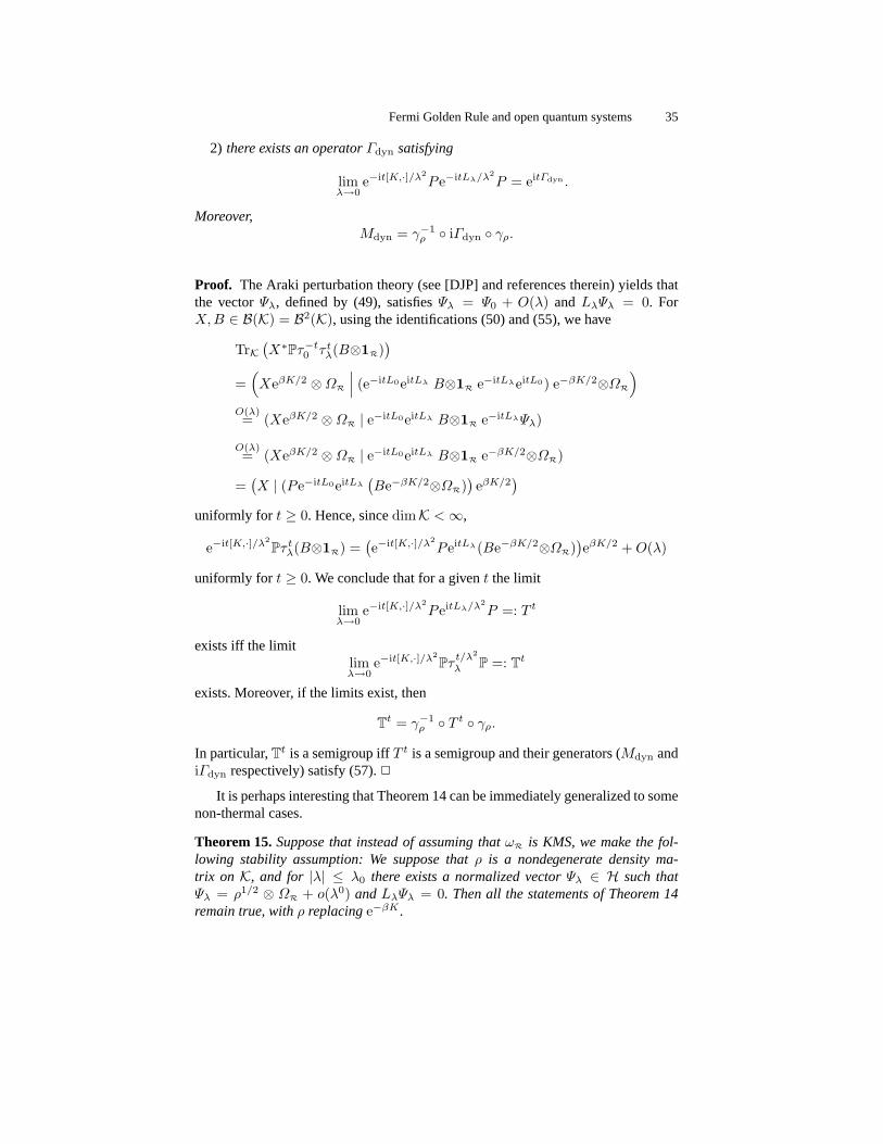
ρ iΓdyn γρ.
Proof. The Araki perturbation theory (see [DJP] and references therein) yields thatthe vectorΨλ, defined by (49), satisfiesΨλ = Ψ0 + O(λ) and LλΨλ = 0. ForX, B ∈ B(K) = B2(K), using the identifications (50) and (55), we have
TrK(X∗Pτ−t
0 τ tλ(B⊗1R)
)=
(XeβK/2 ⊗ΩR
∣∣∣ (e−itL0eitLλ B⊗1R e−itLλeitL0) e−βK/2⊗ΩR
)O(λ)= (XeβK/2 ⊗ΩR | e−itL0eitLλ B⊗1R e−itLλΨλ)
O(λ)= (XeβK/2 ⊗ΩR | e−itL0eitLλ B⊗1R e−βK/2⊗ΩR)
=(X | (P e−itL0eitLλ
(Be−βK/2⊗ΩR)
)eβK/2
)uniformly for t ≥ 0. Hence, sincedimK < ∞,
e−it[K,·]/λ2Pτ t
λ(B⊗1R) =(e−it[K,·]/λ2
P eitLλ(Be−βK/2⊗ΩR))eβK/2 + O(λ)
uniformly for t ≥ 0. We conclude that for a givent the limit
limλ→0
e−it[K,·]/λ2P eitLλ/λ2
P =: T t
exists iff the limitlimλ→0
e−it[K,·]/λ2Pτ
t/λ2
λ P =: Tt
exists. Moreover, if the limits exist, then
Tt = γ−1ρ T t γρ.
In particular,Tt is a semigroup iffT t is a semigroup and their generators (Mdyn andiΓdyn respectively) satisfy (57).2
It is perhaps interesting that Theorem 14 can be immediately generalized to somenon-thermal cases.
Theorem 15.Suppose that instead of assuming thatωR is KMS, we make the fol-lowing stability assumption: We suppose thatρ is a nondegenerate density ma-trix on K, and for |λ| ≤ λ0 there exists a normalized vectorΨλ ∈ H such thatΨλ = ρ1/2 ⊗ ΩR + o(λ0) andLλΨλ = 0. Then all the statements of Theorem 14remain true, withρ replacinge−βK .

36 Jan Derezinski and Rafał Fruboes
Let us return to the thermal case. It is well known [A, FGKV] that in this casethe Davies generator satisfies the Detailed Balance Condition. We will see that thisfact is essentially equivalent to Relation (57).
Theorem 16.Suppose thatωR is a (τR, β)-KMS state and Assumption 6.1 holds.Then the Davies generatorM satisfies DBC fore−βK both in the standard senseand in the sense of AFGKV.
Proof. Recall that the operatorγρ defined in (58) is unitary fromB2(ρ)(K) toB2(K).
Recall also that in the thermal case
M = γ−1ρ iΓ γρ.
Hence,M∗(ρ) = −γ−1
ρ iΓ ∗ γρ.
Thus,12i (M −M∗(ρ)) = γ−1
ρ 12 (Γ + Γ ∗) γρ
= γ−1ρ [∆R, ·] γρ = [∆R, ·],
(where∆R will be defined in the next subsection). This proves DBC in the sense ofAFGKV.
By Theorem 11 and the fact thatρ is proportional toe−βK , for anyz ∈ C wehave
M(B) = ρzM(ρ−zBρz)ρ−z.
Therefore, by Theorem 10, the DBC in the sense of AFGKV is equivalent to thestandard DBC.2
6.4 Explicit formula for the Davies generator
In this subsection we suppose that Assumption 6.1 is true and we describe an explicitformula for the Davies generatorM .
We introduce the following notation for the set of allowed transition frequenciesand the set of allowed transition frequencies fromk ∈ spK:
F := k1 − k2 : k1, k2 ∈ spK = sp[K, ·], Fk := k − k1 : k1 ∈ spK.
Let |Ω) denote the map
C 3 z 7→ |Ω)z := zΩ ∈ HR.
Then1K⊗|Ω) ∈ B(K,K ⊗HR). Set
v := V 1K⊗|Ω)
Note thatv belongs toB(K,K ⊗HR). We also define

Fermi Golden Rule and open quantum systems 37
vk1,k2 := 1k1(K)⊗1R v 1k2(K);
vp :=∑
k∈spK
vk,k−p;
∆ =∑
k∈spK
∑p∈Fk
(v∗)k,k−p1⊗(p + i0− LR)−1vk−p,k
=∑
p∈F(vp)∗1⊗(p + i0− LR)−1vp.
The real and the imaginary part of∆ are given by
∆R := 12 (∆ + ∆∗) =
∑k∈spK
∑p∈Fk
(v∗)k,k−p1⊗P(p− LR)−1vk−p,k
=∑
p∈F(vp)∗1⊗P(p− LR)−1vp;
∆I := 12i (∆−∆∗) = π
∑k∈spK
∑p∈Fk
(v∗)k,k−p1⊗δ(p− LR)vk−p,k
= π∑
p∈F(vp)∗1⊗δ(p− LR)vp;
Note that∆I ≥ 0. Below we give four explicit formulas for the Davies generator inthe Heisenberg picture:
M(B) = i(∆B −B∆∗)
+2π∑
p∈F(vp)∗ B⊗δ(p− LR)vp
= i∑
p∈F(vp)∗1⊗(p− i0− LR)−1 (vpB −B⊗1Rvp)
−i∑
p∈F(B(vp)∗ − (vp)∗B⊗1R)1⊗(p + i0− LR)−1vp
= i[∆R, B]
+π∑
p∈F(vp)∗1⊗δ(p− LR) (B⊗1Rvp − vpB)
+π∑
p∈F((vp)∗B⊗1R −B(vp)∗)1⊗δ(p− LR)vp
= i∑
k∈spK
∑p∈Fk
∞∫0
1k(K)(Ω|V 1k−p(K)τ s0 (V )Ω)1k(K)Bds
−i∑
k∈spK
∑p∈Fk
0∫−∞
B1k(K)(Ω|V 1k−p(K)τ s0 (V )Ω)1k(K)ds
+2π∑
k,k′∈spK
p∈Fk∩Fk′
∞∫−∞
1k(K)(Ω|V 1k−p(K)B1k′−p(K)τ s0 (V )Ω)1k′(K)ds.

38 Jan Derezinski and Rafał Fruboes
The first expression on the right has the standard form of a Lindblad-Kossakowskigenerator (39). The second expression can be used in a characterization of the kernelof M . In particular, it implies immediately that1K ∈ KerM . The third expressionshows the splitting ofM into a reversible part and an irreversible part. The fourthexpression uses uses time-dependent quantities and is analoguous to formulas ap-pearing often in the physics literature.
6.5 Explicit formulas for LSO for the Liouvillean
In this subsection we suppose that Assumption 6.2 is true and we describe an explicitformula foriΓ , the LSO for the Liouvillean.
Recall thatπ denotes the standard representation ofM andLR is the Liouvilleanof the free reservoir dynamicsτR. Let L0
R denote the Liouvillean of the modulardynamics for the stateωR. The fact thatωR is stationary forτ t
R implies that the twoLiouvilleans commute:
eitLReisL0R = eisL0
ReitLR , t, s ∈ R.
The following identities follow from the modular theory and will be useful in ourexplicit formulas forΓ :
Proposition 1. The following identities are true forB ∈ B2(K):
π(V ) B⊗ΩR = vB,
Jπ(V )J B⊗ΩR = B⊗eL0R/2v.
Moreover, ifB1, B2 ∈ B2(K) andΦ ∈ HR, then
(B1 ⊗ Φ|vB2) = (eL0R/2vB1|B2 ⊗ JRΦ). (59)
Proof. To prove the second identity we note that
J B⊗ΩR = B∗⊗ΩR,
Jπ(V )B∗⊗ΩR = eL0R/2B⊗π(V )ΩR.
To see (59), we note that it is enough to assume thatΦ = A′ΩR, whereA′ ∈π(MR)′ andπ(MR)′ denotes the commutant ofπ(MR). Then
(B1 ⊗ Φ|vB2) = (B1 ⊗A′ΩR|π(V )B2 ⊗ΩR)
= (π(V )B1 ⊗ΩR|B2 ⊗A′∗ΩR)
= (vB1|B2 ⊗ eL0R/2JRA′ΩR).
2
Note that if we compare (59) with the definition of the?-operation (37), and ifwe make the identificationΦ = JRΦ, then we see that (59) can be rewritten as

Fermi Golden Rule and open quantum systems 39
v? = eL0R/2v.
The LSO for the Liouvillean equals
iΓ (B) = i∆B − iB∆∗
+2π∑
p∈F(vp)∗ B⊗δ(p− LR)eL0
R/2vp.(60)
Note that the term on the second line of (60) is completely positive. Therefore, (60)is in the Lindblad-Kossakowski form. HenceeitΓ is a c.p. semigroup. This completesthe proof of Theorem 12.
Let us splitΓ into its real and imaginary part:
ΓR :=12(Γ + Γ ∗), Γ I :=
12i
(Γ − Γ ∗).
(Γ ∗ is defined using the natural scalar product inB2(K)). Then the real part is givenby
ΓR(B) = [∆R, B]. (61)
The imaginary part equals
Γ I = π∑
p∈F(vp)∗1⊗δ(p− LR)
(B⊗eL0
R/2vp − vpB)
+π∑
p∈F
((vp)∗B⊗eL0
R/2 −B(vp)∗)1⊗δ(p− LR)vp.
(62)
Another useful formula forΓ I represents it as a quadratic form:
TrB1ΓI(B2)
= π∑
p∈FTr(vpB1 −B1⊗eL0
R/2vp)∗1⊗δ(p− LR)(vpB2 −B2⊗eL0R/2vp).
(63)
To see (63) we note the following identities:
(vp)∗1⊗δ(p− LR)vp = TrHR1⊗δ(p− LR)eL0R vp(vp)∗,
(vp)∗B⊗δ(p− LR)eL0R/2vp = TrHR1⊗δ(p− LR)eL0
R/2vp B(vp)∗,
which follow from (59).The study of the kernel ofΓ I is important in applications based on the Spectral
Fermi Golden Rule. The identity (63) is very convenient for this purpose. It was firstdiscovered in the context of Pauli-Fierz systems in [DJ2].
In the thermal case (63) can be transformed into
TrB1ΓI(B2) = π
∑p∈F
Tre−βK(vpB1eβK/2 −B1eβK/2⊗1R vp)∗
×1⊗δ(p− LR)(vpB2eβK/2 −B2eβK/2⊗1R vp).(64)
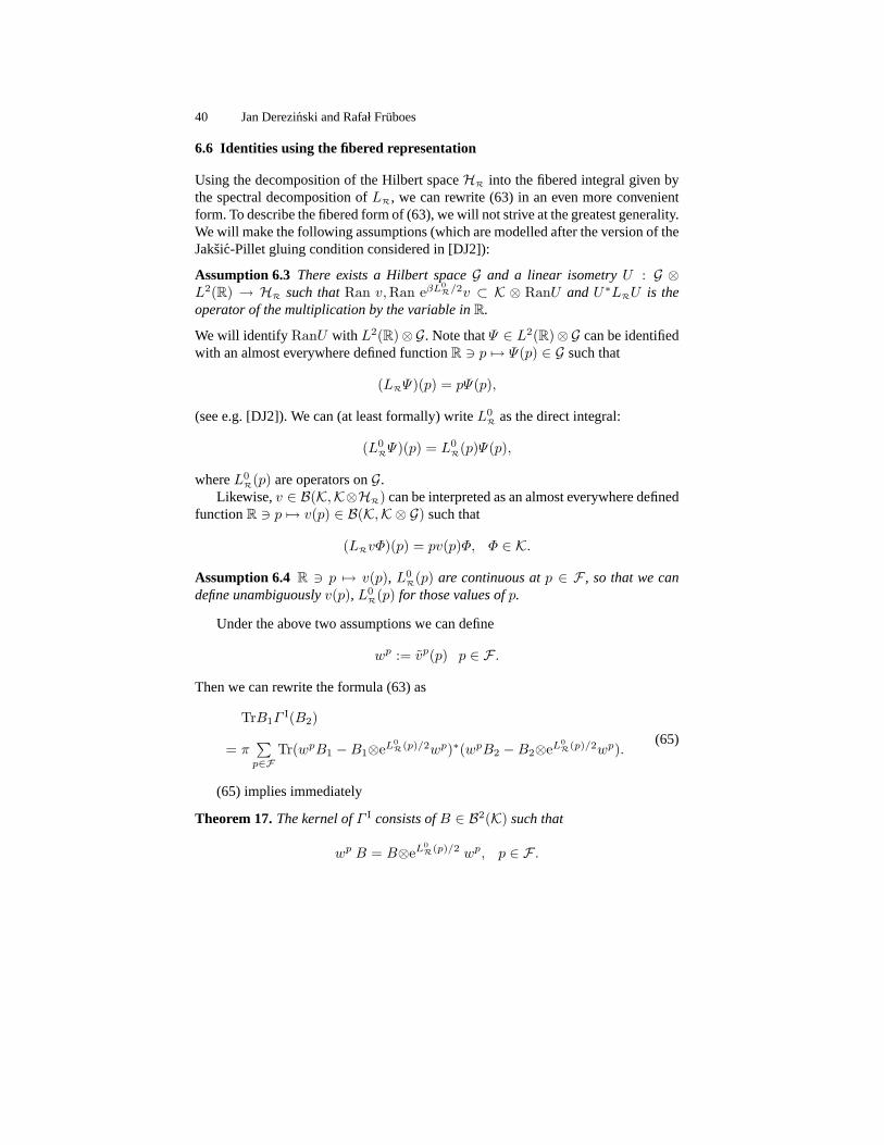
40 Jan Derezinski and Rafał Fruboes
6.6 Identities using the fibered representation
Using the decomposition of the Hilbert spaceHR into the fibered integral given bythe spectral decomposition ofLR, we can rewrite (63) in an even more convenientform. To describe the fibered form of (63), we will not strive at the greatest generality.We will make the following assumptions (which are modelled after the version of theJaksic-Pillet gluing condition considered in [DJ2]):
Assumption 6.3 There exists a Hilbert spaceG and a linear isometryU : G ⊗L2(R) → HR such thatRan v,Ran eβL0
R/2v ⊂ K ⊗ RanU and U∗LRU is theoperator of the multiplication by the variable inR.
We will identify RanU with L2(R)⊗G. Note thatΨ ∈ L2(R)⊗G can be identifiedwith an almost everywhere defined functionR 3 p 7→ Ψ(p) ∈ G such that
(LRΨ)(p) = pΨ(p),
(see e.g. [DJ2]). We can (at least formally) writeL0R as the direct integral:
(L0RΨ)(p) = L0
R(p)Ψ(p),
whereL0R(p) are operators onG.
Likewise,v ∈ B(K,K⊗HR) can be interpreted as an almost everywhere definedfunctionR 3 p 7→ v(p) ∈ B(K,K ⊗ G) such that
(LRvΦ)(p) = pv(p)Φ, Φ ∈ K.
Assumption 6.4 R 3 p 7→ v(p), L0R(p) are continuous atp ∈ F , so that we can
define unambiguouslyv(p), L0R(p) for those values ofp.
Under the above two assumptions we can define
wp := vp(p) p ∈ F .
Then we can rewrite the formula (63) as
TrB1ΓI(B2)
= π∑
p∈FTr(wpB1 −B1⊗eL0
R(p)/2wp)∗(wpB2 −B2⊗eL0R(p)/2wp).
(65)
(65) implies immediately
Theorem 17.The kernel ofΓ I consists ofB ∈ B2(K) such that
wp B = B⊗eL0R(p)/2 wp, p ∈ F .

Fermi Golden Rule and open quantum systems 41
Note that Theorem 17 implies that genericallyKerΓ I = 0. Therefore, for ageneric open quantum system, if the Spectral Fermi Golden Rule can be applied,then the LiouvilleanLλ has no point spectrum for small nonzeroλ. Therefore, forthe sameλ, theW ∗-dynamical system(M, τλ) has no invariant normal states.
Identities (63), (65) and Theorem 17 are generalizations of similar statementsfrom [DJ2]. In [DJ2] the reader will find their rigorous application to Pauli-Fierzsystems.
If ωR is a(τR, β)-KMS state, we can transform (65) as follows:
TrB1ΓI(B2) = π
∑p∈F
Tr e−βK(wp B1eβK/2 −B1eβK/2⊗1R wp)∗
×(wp B2eβK/2 −B2eβK/2⊗1R wp).(66)
Following [DJ2], define
N := C : wp C = C⊗1R wp, p ∈ F. (67)
Repeating the arguments of [DJ2] we get
Theorem 18. 1) N is a∗-algebra invariant wrteitK · e−itK and containingC1.2) The kernel ofΓ I consists ofe−βK/2C with C ∈ N .
Theorem 18 implies that in a thermal case, generically,KerΓ I = 0. There-fore, if the Spectral Fermi Golden Rule can be applied, for a generic open quantumsystem, for small nonzeroλ, the LiouvilleanLλ has no point spectrum except fora nondegenerate eigenvalue at zero. Therefore, for the sameλ, theW ∗-dynamicalsystem(M, τλ) has a unique stationary normal state.
Again, Identity (66) and Theorem 18 are generalizations of similar statementsfrom [DJ2], where they were used to study the return to equilibrium for thermalPauli-Fierz systems.
7 Fermi Golden Rule for a composite reservoir
In this section we describe a small quantum system interacting with several reser-voirs. We will assume that the reservoirsR1, . . . ,Rn do not interact directly—theyinteract with one another only through the small systemS. We will compute bothkinds of the LSO for the composite system. We will see that it is equal to the sum ofthe LSO’s corresponding to the interaction ofS with a single reservoirRi.
Our presentation is divided into 3 subsections. The first uses the framework ofSection 2, the second—that of Section 5 and the third—that of Section 6.
7.1 LSO for a sum of perturbations
Let X be a Banach space. LetP1, . . . , Pn be projections of norm 1 onX such thatPiPj = PiPj . Let L0 be the generator of a group of isometries such thatL0Pi =
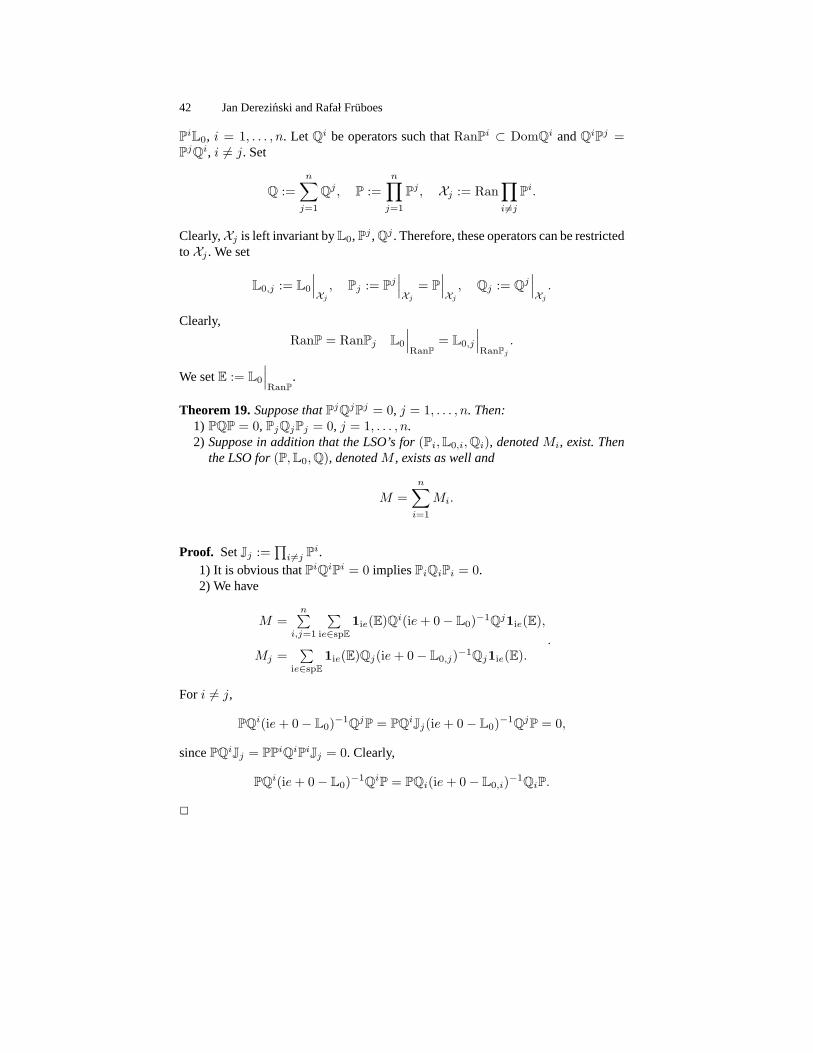
42 Jan Derezinski and Rafał Fruboes
PiL0, i = 1, . . . , n. Let Qi be operators such thatRanPi ⊂ DomQi andQiPj =PjQi, i 6= j. Set
Q :=n∑
j=1
Qj , P :=n∏
j=1
Pj , Xj := Ran∏i 6=j
Pi.
Clearly,Xj is left invariant byL0, Pj , Qj . Therefore, these operators can be restrictedtoXj . We set
L0,j := L0
∣∣∣Xj
, Pj := Pj∣∣∣Xj
= P∣∣∣Xj
, Qj := Qj∣∣∣Xj
.
Clearly,
RanP = RanPj L0
∣∣∣RanP
= L0,j
∣∣∣RanPj
.
We setE := L0
∣∣∣RanP
.
Theorem 19.Suppose thatPjQjPj = 0, j = 1, . . . , n. Then:1) PQP = 0, PjQjPj = 0, j = 1, . . . , n.2) Suppose in addition that the LSO’s for(Pi, L0,i, Qi), denotedMi, exist. Then
the LSO for(P, L0, Q), denotedM , exists as well and
M =n∑
i=1
Mi.
Proof. SetJj :=∏
i 6=j Pi.1) It is obvious thatPiQiPi = 0 impliesPiQiPi = 0.2) We have
M =n∑
i,j=1
∑ie∈spE
1ie(E)Qi(ie + 0− L0)−1Qj1ie(E),
Mj =∑
ie∈spE1ie(E)Qj(ie + 0− L0,j)−1Qj1ie(E).
.
For i 6= j,
PQi(ie + 0− L0)−1QjP = PQiJj(ie + 0− L0)−1QjP = 0,
sincePQiJj = PPiQiPiJj = 0. Clearly,
PQi(ie + 0− L0)−1QiP = PQi(ie + 0− L0,i)−1QiP.
2
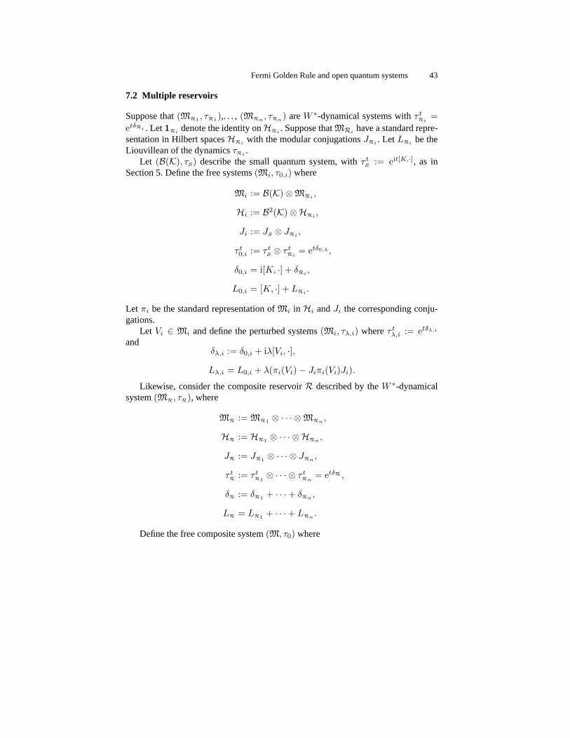
Fermi Golden Rule and open quantum systems 43
7.2 Multiple reservoirs
Suppose that(MR1 , τR1),. . . , (MRn , τRn) areW ∗-dynamical systems withτ tRi
=etδRi . Let1Ri
denote the identity onHRi. Suppose thatMRi
have a standard repre-sentation in Hilbert spacesHRi with the modular conjugationsJRi . Let LRi be theLiouvillean of the dynamicsτRi .
Let (B(K), τS) describe the small quantum system, withτ tS := eit[K,·], as in
Section 5. Define the free systems(Mi, τ0,i) where
Mi := B(K)⊗MRi,
Hi := B2(K)⊗HRi,
Ji := JS ⊗ JRi,
τ t0,i := τ t
S ⊗ τ tRi
= etδ0,λ ,
δ0,i = i[K, ·] + δRi,
L0,i = [K, ·] + LRi.
Let πi be the standard representation ofMi in Hi andJi the corresponding conju-gations.
Let Vi ∈ Mi and define the perturbed systems(Mi, τλ,i) whereτ tλ,i := etδλ,i
andδλ,i := δ0,i + iλ[Vi, ·],
Lλ,i = L0,i + λ(πi(Vi)− Jiπi(Vi)Ji).
Likewise, consider the composite reservoirR described by theW ∗-dynamicalsystem(MR, τR), where
MR := MR1 ⊗ · · · ⊗MRn ,
HR := HR1 ⊗ · · · ⊗ HRn,
JR := JR1 ⊗ · · · ⊗ JRn,
τ tR := τ t
R1⊗ · · · ⊗ τ t
Rn= etδR ,
δR := δR1 + · · ·+ δRn,
LR = LR1 + · · ·+ LRn.
Define the free composite system(M, τ0) where
44 Jan Derezinski and Rafał Fruboes
M := B(K)⊗MR,
H := B2(K)⊗HR,
J = JS ⊗ JR,
τ t0 := τ t
S ⊗ τ tR = etδ0 ,
δ0 = i[K, ·] + δR,
L0 = [K, ·] + LR.
Let π be the standard representation ofM in H.SetV = V1 + · · · + Vn. The perturbed composite system describing the small
systemS interacting with the composite reservoirR is (M, τλ), whereτ tλ := etδλ ,
δλ := δ0 + iλ[V, ·],
Lλ := L0 + λ(π(V )− Jπ(V )J)..
7.3 LSO for the reduced dynamics in the case of a composite reservoir
Suppose that the reservoir dynamicsτRihave stationary statesωRi
. We introduce aprojection of norm one inM, denotedPi, such that
Pi(B ⊗A1⊗, · · · ⊗Ai ⊗ · · · ⊗An) = ωRi(Ai)B ⊗A1 ⊗ · · · ⊗ 1Ri
⊗ · · · ⊗An.
SetP :=∏n
i=1 Pi. The projectionPi restricted toMi (which can be viewed as asubalgebra ofM) is denoted byPi. Explicitly,
Pi(B ⊗Ai) = ωRi(Ai)B ⊗ 1Ri
.
Assume thatωRi(Vi) = 0 for i = 1, . . . , n.
Note that we can apply the formalism of Subsection 7.1, where the Banach spaceisX is M, the projectionsPi arePi, the generator of an isometric dynamicsL0 is δ0
and the perturbationsQi arei[Vi, ·]. Clearly,Xi can be identified withMi andRanPwith B(K).
We obtain the LSO for(P, δ0, i[V, ·]), denotedM , and the LSO’s for(Pi, δ0,i, i[Vi, ·]),denotedMi. By Theorem 19, we have
M =n∑
i=1
Mi,
7.4 LSO for the Liovillean in the case of a composite reservoir
Let ΩRi be the standard vector representative ofωRi . We define the orthogonal pro-jection inB(H)

Fermi Golden Rule and open quantum systems 45
P i := 1B2(K) ⊗ 1R1 ⊗ · · · ⊗ |ΩRi)(ΩRi
| ⊗ · · · ⊗ 1Rn.
The projectionP i restricted toHi is denoted byPi and equals
Pi = 1B2(K) ⊗ |ΩRi)(ΩRi |.
SetP =∏n
i=1 P i.We can apply the formalism of Subsection 7.1, where the Banach space isX is
H, the projectionsPi areP i, the generator of an isometric dynamicsL0 is iL0 andthe perturbationsQi are i(Vi − JiViJi). Clearly,Xi can be identified withHi andRanP with B2(K) (which as a vector space coincides withB(K)).
We obtain the LSO for(P, iL0, i(V − JV J)), denotediΓ , and the LSO for(Pi, iL0,i, i(Vi − JiViJi)), denotediΓi. By Theorem 19, we have
iΓ =n∑
i=1
iΓi.
The following theorem follows from obvious properties of negative operators:
Theorem 20.Suppose that for somei 6= j, dim KerΓ Ii = dim KerΓ I
j = 1 andKerΓ I
i 6= KerΓ Ij . ThenKerΓ = 0.
Corollary 1. Suppose that for somei 6= j, the statesωRiandωRj
are (τRi, βi) and
(τRj, βj)-KMS. LetNi andNj be the corresponding∗-algebras defined as in (67).
Suppose thatβi 6= βj andN ′i = N ′
j = C1. ThenKerΓ = 0.
If we can apply the Spectral Fermi Golden Rule, then under the assumptions of1, for sufficiently small nonzeroλ, Lλ has no point spectrum. Consequently, for thesameλ, the system(Mλ, τλ), has no invariant normal states.
A Appendix – one-parameter semigroups
In this section we would like to discuss some concepts related to one-parametersemigroups of operators in Banach spaces, which are used in our lectures. Eventhough the material that we present is quite standard, we could not find a referencethat presents all of it in a convenient way. Most of it can be found in [BR1]. Lesspedantic readers may skip this appendix altogether.
Let X be a Banach space. Recall that[0,∞[3 t 7→ U(t) ∈ B(X ) is calleda 1-parameter semigroup iffU(0) = 1 andU(t1)U(t2) = U(t1 + t2). If [0,∞[is replaced withR, then we speak about a one-parameter group instead of a one-parameter semigroup.
We say thatU(t) is a strogly continuous semigroup (or aC0-semigroup) iff foranyΦ ∈ X , t 7→ U(t)Φ is continuous. EveryC0-semigroup possesses its generator,that is the operatorA defined as follows:
Φ ∈ DomA ⇔ limt0
t−1(U(t)− 1)Φ =: AΦ exists.

46 Jan Derezinski and Rafał Fruboes
The generator is always closed and densely defined and uniquely determines thesemigroup. We writeU(t) = etA.
Recall also the following well known characterization of contractive semigroups:
Theorem 21.The following conditions are equivalent:1) etA is contractive for allt ≥ 0.2) A is densely defined,spA ⊂ z ∈ C : Rez ≤ 0 and‖(z−A)−1‖ ≤ (Rez)−1
for Rez > 0.3) (i) A is densely defined and for somez+ with Rez+ > 0, z+ 6∈ spA,
(ii) A is dissipative, that is for anyΦ ∈ DomA there existsξ ∈ X ∗ with(ξ|Φ) = ‖Φ‖ and(ξ|AΦ) ≤ 0.
Moreover, ifA is bounded, then we can omit(i) in 3).
There exists an obvious corollary of the above theorem for groups of isometries:
Theorem 22.The following conditions are equivalent:1) etA is isometric for allt ∈ R.2) A is densely defined,spA ⊂ iR and‖(z −A)−1‖ ≤ |Rez|−1 for Rez 6= 0.3) (i) A is densely defined and for somez± with±Rez± > 0, z± 6∈ spA,
(ii) A is conservative, that is for anyΦ ∈ DomA there existsξ ∈ X ∗ with(ξ|Φ) = ‖Φ‖ andRe(ξ|AΦ) = 0.
Morover, ifA is bounded, then we can omit(i) in (3).
Not all semigroups considered in our lectures areC0-semigroups. An importantrole in our lectures (and in applications to statistical physics) is played by somewhatless knownC∗0 -semigroups. In order to discuss them, first we need to say a few wordsabout dual Banach spaces.
LetX ∗ denote the Banach space dual toX (the space of continuous linear func-tionals onX ). We will use the sesquilinear duality betweenX ∗ andX : the form(ξ|Φ) will be antilinear inξ ∈ X ∗ and linear inΦ ∈ X .
The so-called weak∗ (w∗) topology onX ∗ is defined by the seminorms|(·|Φ)|,whereΦ ∈ X .
The space of w∗ continuous linear operators onX ∗ will be denoted byBw∗(X ∗).Note thatBw∗(X ∗) ⊂ B(X ∗). If A ∈ B(X ), andA∗ is its adjoint, thenA∗ ∈Bw∗(X ∗). Conversely, ifB ∈ Bw∗(X ∗), then there exists a uniqueA ∈ B(X ),sometimes called the preadjoint ofB, such thatB = A∗. Likewise, if A is closedand densely defined onX , thenA∗ is w∗ closed and w∗ densely defined onX ∗.
We say that[0,∞[3 t 7→ W (t) ∈ Bw∗(X ∗) is a w∗ continuous semigroup (ora C∗0 -semigroup) ifft 3 W (t)ξ is w∗ continuous for anyξ ∈ X ∗. Note that ifU(t) is a C0 -semigroup, thenU(t)∗ is a C∗0 -semigroup. Conversely, ifW (t) is aC∗0 -semigroup onX ∗, then there exists a uniqueC0-semigroupU(t) onX such thatW (t) = U(t)∗.
EveryC∗0 -semigroupW (t) possesses its generator, that is the operatorB definedas follows:
ξ ∈ DomB ⇔ w ∗ − limt0
t−1(W (t)− 1)ξ =: Bξ exists.

Fermi Golden Rule and open quantum systems 47
The generator is always w∗-closed and w∗-densely defined and uniquely determinesthe semigroup. We writeW (t) = etB . We have
(etA)∗ = etA∗.
On a reflexive Banach space, e.g. on a Hilbert space, the concepts of aC0- andC∗0 -semigroup coincide. Unfortunately,W ∗-algebras are usually not reflexive. Theyare, however, dual Banach spaces: they are dual to the space of normal function-als. In the context ofW ∗-algebras the w∗-topology is usually called theσ-weak orultraweak topology.
Groups of automorphisms ofW ∗-algebras are rarelyC0-groups. To see this notethat if H is a self-adjoint operator on a Hilbert spaceH, then
t 7→ eitH · e−itH (68)
is always aC∗0 -group onB(H). It is aC0-group (and even a norm continuous group)iff H is bounded, which is usually a very severe restriction.
In the context ofW ∗-algebras,C∗0 groups are usually called (pointwise)σ-weakly continuous groups.C∗0 -groups of∗-automorphisms are often calledW ∗-dynamics.
So far, all the material that we recalled can be found e.g. in [BR1]. Now wewould like to discuss how to define the spectral projection onto a (not necessarilyisolated) eigenvalue of a generator of contractive semigroup. We will see that a fullysatisfactory answer is available for purely imaginary eigenvalues in the case of areflexive Banach spaces. For non-reflexive Banach spaces the situation is much morecomplicated. Our discussion is adapted from [Zs] and partly from [Da3].
LetA be the generator of a contractiveC0-semigroup onX ande ∈ R. Following[Zs], we say thatA is ergodic atie iff
1ie(A) := limξ0
ξ(ξ + ie−A)−1 (69)
exists.Let B be the generator of a contractiveC∗0 -semigroup onX ∗ ande ∈ R. Follow-
ing [Zs], we say thatB is globally ergodic atie iff
1ie(B) := w ∗ − limξ0
ξ(ξ + ie− B)−1 (70)
exists and is w∗-continuous.As we will see from the theorem below, (69) and (70) can be called spectral
projections onto the eigenvalueie.
Theorem 23.LetA, B ande ∈ R be as above.1) If A is ergodic atie, then1ie(A) is a projection of norm1 such that
Ran1ie(A) = Ker(A− ie), Ker1ie(A) = (Ran (A− ie))cl .
48 Jan Derezinski and Rafał Fruboes
2) On a reflexive Banach space, we have always the ergodic property for all gen-erators of contractive semigroups and allie ∈ iR.
3) If B is globally ergodic atie, then1ie(B) is a w∗-continuous projection ofnorm1 such that
Ran1ie(B) = Ker(B − ie), Ker1ie(B) = (Ran (A− ie))w∗cl.
4) A is ergodic atie iff A∗ is globally ergodic at−ie and
1ie(A)∗ = 1−ie(A∗).
1) and 2) are proven in [Da3] Theorem 5.1 and Corollary 5.2. 3) and 4) can beproven by adapting the arguments of [Zs] Theorem 3.4 and Corollary 3.5.
As an ilustration of the above concepts consider theW ∗-dynamics (68). Clearly,it is a group of isometries and the spectrum of its generatori[H, ·] is contained iniR.If H possesses only point spectrum, theni[H, ·] is globally ergodic for anyie ∈ iR.In fact, we have the following formula for
1ie(i[H, ·])(C) =∑x∈R
1x+e(H)C1x(H).
Note thati[H, ·] always possesses an eigenvalue0 and the corresponding eigen-vectors are all operators commuting withH. It is never globally ergodic at0 if Hhas some continuous spectrum.
References
[AJPP] Aschbacher, W., Jaksic, V., Pautrat, Y., Pillet, C.-A.: Introduction to non-equilibriumquantum statistical mechanics. Grenoble lecture notes.
[A] Alicki, R.: On the detailed balance condition for non-hamiltonian systems, Rep. Math.Phys. 10 (1976) 249
[AL] Alicki, R., Lendi, K.: Quantum dynamical semigroups and applications, Lecture Notesin Physics no 286, Springer 1991
[BR1] Brattelli, O., Robinson D. W.:Operator Algebras and Quantum Statistical Mechanics,Volume 1. Springer-Verlag, Berlin, second edition 1987.
[BR2] Brattelli, O., Robinson D. W.:Operator Algebras and Quantum Statistical Mechanics,Volume 2. Springer-Verlag, Berlin, second edition 1996.
[BFS1] Bach, V., Frohlich, J., Sigal, I.: Quantum electrodynamics of confined non-relativisticparticles, Adv. Math.137, 299 (1998).
[BFS2] Bach, V., Frohlich, J., Sigal, I.: Return to equilibrium. J. Math. Phys.41, 3985 (2000).[Da1] Davies, E. B.: Markovian master equations. Commun. Math. Phys.39, 91 (1974).[Da2] Davies, E. B.: Markovian master equations II. Math. Ann.219, 147 (1976).[Da3] Davies, E. B.: One parameter semigroups, Academic Press 1980[DJ1] Derezinski, J., Jaksic, V.: Spectral theory of Pauli-Fierz operators. J. Func. Anal.180,
243 (2001).[DJ2] Derezinski, J., Jaksic, V.: Return to equilibrium for Pauli-Fierz systems. Ann. Henri
Poincare4, 739 (2003).

Fermi Golden Rule and open quantum systems 49
[DJ3] Derezinski, J., Jaksic, V.: On the nature of Fermi golden rule for open quantum sys-tems, J. Statist. Phys.116(2004), 411 (2004).
[DJ4] Derezinski, J., Jaksic, V.: In preparation.[Di] Dirac, P.A.M.: The quantum theory of the emission and absorption of radiation. Proc.
Royal Soc. London, Series A114, 243 (1927).[DJP] Derezinski, J., Jaksic, V., Pillet, C. A.:Perturbation theory ofW ∗-dynamics, Liouvil-
leans and KMS-states, to appear in Rev. Math. Phys[FGKV] Frigerio, A., Gorini, V., Kossakowski A., Verri, M.: Quantum detailed balance and
KMS condition, Comm. Math. Phys. 57 (1977) 97-110[DF1] Derezinski, J., Fruboes, R.: Level Shift Operator and 2nd order perturbation theory, to
appear in J. Math. Phys.[DF2] Derezinski, J., Fruboes, R.: Stationary van Hove limit, to appear in J. Math. Phys.[Fe] Fermi, E.: Nuclear Physics, University of Chicago Press, Chicago 1950[GKS] Gorini, V., Kossakowski, A., Sudarshan, E.C.G. Journ. Math. Phys. 17 (1976) 821[Haa] Haake, F.:Statistical treatment of open systems by generalized master equation.
Springer Tracts in Modern Physics66, Springer-Verlag, Berlin, 1973.[JP1] Jaksic, V., Pillet, C.-A.: On a model for quantum friction III. Ergodic properties of the
spin-boson system. Commun. Math. Phys.178, 627 (1996).[JP2] Jaksic, V., Pillet, C.-A.: Spectral theory of thermal relaxation. J. Math. Phys.38, 1757
(1997).[JP3] Jaksic, V., Pillet, C.-A.: From resonances to master equations. Ann. Inst. Henri
Poincare67, 425 (1997).[JP4] Jaksic, V., Pillet, C.-A.: Non-equilibrium steady states for finite quantum systems cou-
pled to thermal reservoirs. Commun. Math. Phys.226, 131 (2002).[JP5] Jaksic, V., Pillet, C.-A.: Mathematical theory of non-equilibrium quantum statistical
mechanics. J. Stat. Phys.108, 787 (2002).[JP6] Jaksic, V., Pillet, C.-A.: In preparation.[Ka] Kato, T.:Perturbation Theory for Linear Operators, second edition,[KTH] Kubo, R., Toda, M., Hashitsume, N.:Statistical Physics II. Nonequilibrium Statistical
Mechanics.Springer-Verlag, Berlin, 1985.[L] Lindblad, G.: On the generators of quantum dynamical semigroups, Comm. Math.
Phys. 48 (1976) 119-130[M] Merkli, M.: Positive commutators in non-equilibrium quantum statistical mechanics.
Commun. Math. Phys.223, 327 (2001).[LeSp] Lebowitz, J., Spohn, H.: Irreversible thermodynamics for quantum systems weakly
coupled to thermal reservoirs. Adv. Chem. Phys.39, 109 (1978).[Ma1] Majewski, W. A.: Dynamical semigroups in the algebraic formulation of statistical
mechanics, Fortschritte der Physik 32 (1984) 89-133[Ma2] Majewski, W. A.: Journ. Math. Phys. The detailed balance condition in quantum sta-
tistical mechanics 25 (1984) 614[MaSt] Majewski, W. A., Streater, R. F.: Detailed balance and quantum dynamical maps
Journ. Phys. A: Math. Gen. 31 (1998) 7981-7995[VH1] Van Hove, L.: Quantum-mechanical perturbations giving rise to a statistical transport
equation. Physica21 (1955) 517.[VH2] Van Hove, L.: The approach to equilibrium in quantum statitsics. Physica23 (1957)
441.[VH3] Van Hove, L.: Master equation and approach to equilibrium for quantum systems. In
Fundamental problems in statistical mechanics, compiled by E.G.D. Cohen, North-Holand, Amsterdam 1962.

50 Jan Derezinski and Rafał Fruboes
[RS4] Reed, M., Simon, B.:Methods of Modern Mathematical Physics, IV. Analysis of Op-erators, London, Academic Press 1978.
[Sp] Spohn, H.: Entropy production for quantum dynamical semigroups, Journ. Math. Phys.19 (1978) 1227
[St] Stinespring, W. F.: Positive functions onC∗-algebras, Proc. Am. Math. Soc. 6 (1955)211-216
[WW] Weisskopf, V., Wigner, E.: Berechnung der naturlichen Linienbreite auf Grund derDirakschen Lichttheorie, Zeitschrift fur Physik 63 (130) 54
[Zs] Zsido, L.: Spectral and ergodic properties of analytic generators, Journ. ApproximationTheory 20 (1977) 77-138