femtosecond laser tagging characterization of a sweeping
TRANSCRIPT

American Institute of Aeronautics and Astronautics
1
Femtosecond Laser Tagging Characterization of a Sweeping
Jet Actuator Operating in the Compressible Regime
Christopher J. Peters1 and Richard B. Miles2
Princeton University, Princeton, New Jersey, 08544
Ross A. Burns3, Brett F. Bathel4, Gregory S. Jones5 and Paul M. Danehy6
NASA Langley Research Center, Hampton, Virginia, 23681
A sweeping jet (SWJ) actuator operating over a range of nozzle pressure ratios (NPRs)
was characterized with femtosecond laser electronic excitation tagging (FLEET), single hot-
wire anemometry (HWA) and high-speed/phase-averaged schlieren. FLEET velocimetry
was successfully demonstrated in a highly unsteady, oscillatory flow containing subsonic
through supersonic velocities. Qualitative comparisons between FLEET and HWA (which
measured mass flux since the flow was compressible) showed relatively good agreement in
the external flow profiles. The spreading rate was found to vary from 0.5 to 1.2 depending
on the pressure ratio. The precision of FLEET velocity measurements in the external flow
field was poorer (≈25 m/s) than reported in a previous study due to the use of relatively low
laser fluences, impacting the velocity fluctuation measurements. FLEET enabled velocity
measurements inside the device and showed that choking likely occurred for NPR ≥ 2.0, and
no internal shockwaves were present. Qualitative oxygen concentration measurements using
FLEET were explored in an effort to gauge the jet’s mixing with the ambient. The jet was
shown to mix well within roughly four throat diameters and mix fully within roughly eight
throat diameters. Schlieren provided visualization of the internal and external flow fields
and showed that the qualitative structure of the internal flow does not vary with pressure
ratio and the sweeping mechanism observed for incompressible NPRs also probably holds
for compressible NPRs.
Nomenclature
𝑒 = voltage across hot-wire, V
NPR = nozzle pressure ratio, 𝑝inlet
𝑝ambient
𝑇0 = jet total temperature, K
𝑢 = velocity, m/s
𝑥 = streamwise position coordinate, mm
𝑦 = spanwise position coordinate, mm
𝑦1/2 = jet half-width, mm
Δ𝑡 = FLEET time delay, µs
𝜌 = density, kg/m3
𝜏 = period of sweep, s
1 Graduate Student, Mechanical and Aerospace Engineering, D225 E-Quad, Olden Street, AIAA Student Member. 2 Professor Emeritus, Mechanical and Aerospace Engineering, D225 E-Quad, Olden Street, AIAA Fellow. 3 Research Engineer, National Institute of Aerospace, Mail Stop 493, AIAA Member. 4 Research Scientist, Advanced Measurements and Data Systems Branch, Mail Stop 493, AIAA Senior Member. 5 Research Scientist, Configuration Aerodynamics Branch, Mail Stop 267, AIAA Senior Member. 6 Research Scientist, Advanced Measurements and Data Systems Branch, Mail Stop 493, AIAA Associate Fellow.

American Institute of Aeronautics and Astronautics
2
I. Introduction
sweeping jet (SWJ) actuator is an active flow control device without moving parts that discharges a
continuously blowing, spatially oscillating, planar jet when supplied with pressurized gas.1,2 The sweep
frequency and velocity of the jet depend on the ratio of the plenum pressure to the ambient pressure (defined here as
nozzle pressure ratio or NPR). The sweep frequency also depends on the size and geometry of the device. Figure 1
shows an illustration of the device and its internal fluid dynamics at different phases of its oscillation cycle (after
initial startup) as observed in the present study. The sweep mechanism can be briefly described as follows: 1-2)
flow entering the main chamber entrains the surrounding air which generates a low pressure region and causes the
jet to move towards and attach to one of the walls (Coandă effect); some of the flow enters the feedback loop closest
to the jet, 3) flow from this feedback loop begins to strengthen the recirculation bubble (initially formed by flow
separation) in between the wall and attached jet, 4) fed by the feedback loop, the recirculation bubble grows in size
and eventually pushes the jet to other wall to which it attaches (Coandă effect), 5-6) the feedback process begins for
the other wall and its completion marks one oscillation cycle.3 The growth of the recirculation bubble governs the
sweeping motion of the jet.4 We will show that this description of the sweep mechanism based on incompressible
results also applies to a SWJ actuator operating in the compressible regime.
There is considerable interest in sweeping jet actuators as an energy-efficient means of flow control, since they
have been shown to be as effective as steady blowing3 while requiring less airflow.5,6 In one successful flow control
application, SWJs were able to increase the maximum allowable deflection angle for a jetliner’s rudder by delaying
the onset of flow separation. This application allowed a smaller rudder (with less parasitic drag and weight) to
produce the same amount of side force as a larger rudder.6 The Boeing ecoDemonstrator 757 employs a linear array
of SWJs on its vertical stabilizer for this purpose.7 Researchers at NASA Langley Research Center desire to use
SWJs to control the shock location and wake filling on a transonic wing during cruise. Steady blowing
configurations showed drag improvements for off-design cruise Mach numbers for a state-of-the art wing.8 These
improvements are related to moving the outboard shock aft of the baseline location by as much as 5% without
increasing the shock strength. The added momentum also reduces the wake deficit. Both of these phenomena imply
a reduced drag. This motivates the current study of sweeping jets operating at cruise Mach numbers greater than 0.8
(i.e., in the compressible regime).9
Direct quantitative measurements of supersonic (highly compressible) sweeping jets are limited, and no internal
velocity measurements of a supersonic sweeping jet have been reported.1 Such measurements are particularly
difficult in this internal flow because probes would block the flow and optical methods like particle image
velocimetry (PIV) and Rayleigh scattering suffer from interference from laser light scattering off of windows and
surfaces or seed particles adhering to surfaces (for PIV). Numerical simulations10 and high-speed schlieren
imaging11 of supersonic sweeping jets have been performed, but internal velocity measurements have been restricted
to subsonic (incompressible) sweeping jets.2,3,12
Femtosecond laser electronic excitation tagging (FLEET) is an unseeded molecular tagging technique that can
enable nonintrusive measurements of the internal and external flow of the SWJ actuator irrespective of its operating
regime. FLEET velocimetry is a versatile, easy-to-implement technique (requiring only a single laser and a single
camera) that can be used to study a wide range of flows, including turbulent,13 cryogenic,14 high-speed,15
combusting,16 as well the highly unsteady, subsonic/supersonic flow emanating from a sweeping jet actuator.
FLEET relies on a focused, femtosecond laser pulse to excite and subsequently dissociate molecular nitrogen.17,18
The atomic nitrogen recombines (through a three-body process) into excited molecular nitrogen, which fluoresces
primarily between 520 and 780 nm.19 Although the fluorescence is short-lived, the three-body recombination
process is relatively slow, and the resulting signal is long-lived. In air, signals lasting tens of microseconds after the
exciting laser pulse have been reported.16 Tagged regions appear as luminescent lines written in the air, whose
position and intensity can be tracked by a time-delayed, fast-gated camera. Velocities are determined by measuring
the displacement that occurs during the time delay. Since the primary FLEET signal is non-resonant with the initial
excitation, and the data acquisition is delayed from the laser pulse, FLEET circumvents any optical interference
from scattered light that challenge scattering-based techniques. There is also a possibility of providing simultaneous
concentration measurements in order to gauge the quality of mixing.20 Mixing is potentially important for
mitigating the deleterious effects of shockwave boundary layer interactions (e.g., flow separation) that occur at off-
design Mach numbers.
In this paper, we seek to study the internal and external flow field of a sweeping jet actuator operating in the
compressible flow regime using FLEET. The goals are: 1) to examine the external flow field characteristics (e.g.,
sweep angle and velocity) and internal flow features (e.g., choking and presence of shockwaves) as they pertain to
possible flow control applications, and 2) to demonstrate FLEET as a velocimetry technique suitable for measuring
A

American Institute of Aeronautics and Astronautics
3
highly unsteady, oscillatory flows having a wide dynamic range of velocities. To this end, FLEET will be
qualitatively compared to single hot-wire anemometry (HWA) in the external flow field. High-speed and phase-
averaged schlieren will provide whole-field visualization and phase information about the jet. Furthermore, the
possibility of simultaneously measuring concentration (to estimate the jet’s mixing with the quiescent air) will be
explored.
Figure 1. Diagram of the sweeping jet actuator at six phases of its oscillation cycle. The diagram is modeled
after the diagrams in Refs. 5, 21, and 22, but improved based upon findings from this paper. Phases 1 through 6
correspond approximately to 0.2𝜏, 0.3𝜏, 0.5𝜏, 0.7𝜏, 0.8𝜏, and 1.0𝜏, respectively, where 𝜏 is the SWJ’s period.
II. Experimental Setup and Technique
A. Configuration of Sweeping Jet Actuator
A transparent sweeping jet actuator amenable to optical measurements was constructed with an internal
geometry (see Figure 1) similar to those being proposed for transonic flow control. The throat was approximately
square with a width around 3.2 mm. The flow field was assumed to be predominantly planar since the out-of-plane
depth was narrow relative to the streamwise length. External measurements of the spanwise velocity profile were
made by FLEET and HWA in the plane of the jet at downstream distances of 2.5, 12.7, 25.4 and 50.8 mm from the
exit. At each distance, the SWJ was operated with compressed air at pressure ratios of 1.4, 1.8, 2.0, 2.5 and 3.0.
Extensive testing with other SWJ actuators revealed that these distances and NPRs were sufficient to characterize
the operating behavior of the device. For the internal measurements, pure nitrogen was used instead of air at the
same pressure ratios. The concentration measurements were performed with nitrogen at the downstream distances
listed above for NPRs of 1.4, 1.8, 2.0 and 2.5, but the supply pressure limited the maximum achievable pressure
ratio to about 2.8, as noted on the plots. Each NPR was associated with a dominant fundamental acoustic frequency
as measured by a microphone (G.R.A.S. 40PP CCP Free-field QC Microphone) acquiring at a rate of 51.2 kHz.
Figure 2 shows these data with the maximum observed frequency just below 1 kHz.
Figure 2. Dominant fundamental acoustic frequency as function of nozzle pressure ratio.
0
125
250
375
500
625
750
875
1000
1.00 1.25 1.50 1.75 2.00 2.25 2.50 2.75 3.00
Do
min
an
t F
req
uen
cy (
Hz)
Nozzle Pressure Ratio

American Institute of Aeronautics and Astronautics
4
B. Measurement Systems and Methods
1. FLEET Velocimetry and Concentration Measurement
A regeneratively-amplified Ti:sapphire laser system (Spectra-Physics® Solstice® one-box ultrafast amplifier) was
used to generate the FLEET emission in both air and pure nitrogen. The system produced ≈70 fs duration laser
pulses centered at 800 nm at a repetition rate of 1 kHz. An ultrafast variable beam attenuator (Newport VA-800)
enabled the laser pulse energy to be reduced from its maximum of 3.5 mJ. A power meter (Coherent 210) facilitated
measurement of the beam energy after passage through the optical setup. Focusing and steering of the beam were
accomplished with ultrafast anti-reflective lenses and ultrafast mirrors, respectively. For the external measurements,
a beam with a pulse energy of 2.0 mJ (2.8 mJ for the concentration measurements) was focused by a 1-m focal
length (FL) lens. Figure 3 illustrates the orientation of the FLEET reference line and typical single-shot delayed
lines for the external measurements. The delayed lines show the location of the jet and provide some sense of its
orientation. The 1-m FL lens enabled the writing of a FLEET line roughly 40 mm long across the jet. We intended
for the long line to alleviate the need to pan the field of view to capture the entire spanwise profile and avoid
perturbing the flow via energy deposition; however, writing a long line lowered the laser fluence, the FLEET signal
intensity, and ultimately, adversely affected the measurement precision. This effect is discussed in more detail in
the Appendix. The reduced signal intensity is evident along the edges of FLEET line in the single-shot delayed
images of Figure 3. For the internal measurements, a pulse energy of 0.5 mJ was used along with a shorter focal
length of 125 mm in order to generate a spot rather than a line.
The imaging system consisted of a two-stage intensifier (LaVision HighSpeed IRO) lens-coupled to a high-speed
complementary metal-oxide semiconductor (CMOS) camera (Photron FASTCAM Mini AX200). The camera had a
full-frame (1024 by 1024 pixel) repetition rate of 6.4 kHz. The objective lens on the intensifier was an F-mount
105-mm FL (Nikon NIKKOR) with an aperture range of f/2 to f/16. Except for the concentration measurements, the
intensifier gain was adjusted at the beginning of each run for maximum signal-to-noise (SNR) ratio. The maximum
useable gain setting was that which avoided saturating the camera and avoided introducing an excessive amount of
intensifier-induced spurious noise. Intensifier gate widths of 1 µs (0.5 µs for the concentration measurements) were
used for the external and internal measurements.
Figure 3. FLEET external measurements. (top) Initial spanwise reference line above actuator and (bottom)
typical single-shot delayed lines for 2.5 mm above exit when operating at NPR = 1.4. The single-shot images are
44.2 mm wide.
The camera was unable to frame rapidly without some high spatial frequency ghosting artifacts appearing in
delayed frames. So, the reference (starting) line of tagged molecules and the delayed (displaced) line were measured
separately. The reference line was obtained by shutting the actuator off and then acquiring a series of images.
These images were processed and the results were averaged together to produce a reference line for calculating the
displacement of the delayed line. Such a method is susceptible to errors introduced by facility vibrations or laser
beam misalignment. Displacement calculations were based on the line center as determined by an in-house
Gaussian fitting routine written in MATLAB®. The routine calculated the displacement for each column of pixels in
order to achieve spanwise velocity profiles. The resolution, at best, was roughly 65 µm/pixel (15 pixel/mm) and
2.5 mm
3.2 mm, throat

American Institute of Aeronautics and Astronautics
5
was carefully measured with a dot-card target (i.e., a two-dimensional array of black dots on a white background) of
known spacing. The time delays with respect to the laser pulse were adjusted for each run such that the
displacement was at least several line thicknesses downstream while the signal-to-noise ratio remained acceptable.
The initial intensity and lifetime of the FLEET signal were proportional to the laser fluence.
Concentration measurements (to gauge mixing) were accomplished by exploiting FLEET’s signal dependence
on the mole fraction of oxygen in the gas. The FLEET signal is strongest in pure nitrogen and decreases as the
amount of oxygen in the gas increases since oxygen acts as quenching agent. When imaged at short time delays, the
FLEET signal varies monotonically with the concentration of oxygen.20 Therefore, for the concentration
experiments, we operated the sweeping jet with pure nitrogen. Since the SWJ emits into quiescent air, the pure
nitrogen jet mixes with ambient air and the concentration of oxygen increases in proportion to the amount of mixing
that occurs. Thus, the signal is highest in the unmixed regions and decreases as the mixing increases down to the
point for which the oxygen concentration matches that of air. Signal intensity measurements were based on the
amplitude as determined by the Gaussian fitting procedure. An initial calibration measurement was made in
quiescent air in order to account for spanwise variation in the signal intensity as a result of variations in laser beam
fluence. After normalization by the calibration in air, the FLEET signal intensity was assumed to depend linearly on
oxygen mole fraction. Although this assumption adds uncertainty to the measurement since the relationship is
actually nonlinear, this simplification was done primarily because a proper calibration curve for the signal as a
function of oxygen concentration was not available for our particular setup.20 Simultaneous concentration and
velocity measurements were made by recording two data frames with each laser pulse. The first frame began 75 ns
after the laser pulse and captured the reference location of the line and signal intensity used for the concentration
measurement. The second frame began at the appropriate delay to capture the displaced line. Although
simultaneous velocity and concentration measurements were acquired, rapid framing of the camera (and minimizing
the time between subsequent exposures) led to high-spatial-frequency ghosting artifacts that impaired precise line
center determination in the second frame.
Internal velocity and trajectory measurements were performed by steering the laser beam into the actuator
through the throat to generate a FLEET spot about 2 mm upstream of the throat as depicted in Figure 4 and
operating with compressed nitrogen instead of air for longer FLEET signal lifetimes. The spot advected
downstream, across the field of view such that its position and thus velocity could be measured in each subsequent
frame. The time delay between frames was fixed at 5 µs since the imaging system was operated at 200 kHz in 15-
frame bursts. Two-dimensional cross-correlation was used to determine the displacement of the tagged region in
each frame after the initial frame. Due to the strain and break-up of the tagged region, especially during passage
through the throat (see Figure 4), only a fraction of the 15 frames were usable. The red box approximately
demarcates the domain for which internal results are reported. Note that the advection of the spot deviates from a
purely streamwise motion since the jet is sweeping back and forth within the main channel as shown in Figure 1.
Over 2,600 15-frame bursts were collected for each pressure ratio, generating an ensemble of velocity-position
pairs for each pressure setting. The velocities were then grouped together according to proximity to points on a
uniform grid. The grid size varied between 300 to 500 µm and was selected to be larger than the minimum diameter
of the FLEET spot and to ensure convergence of the sum of squares of mean velocity magnitude. Grouping
velocities into grid points enabled statistics such as mean and mean-subtracted RMS to be performed on the basis of
position. (For a plot of grid’s data point density, see Figure 16 in the Appendix.)
Figure 4. Field of view for FLEET internal measurements and typical images from bursts (frames 1-5 of
15). Flow is left to right. Pure nitrogen at NPR = 2.0. The time delay between frames was 5 µs.
1 2 3 4 5
1 2 3 4 5
1 2 3 4 5

American Institute of Aeronautics and Astronautics
6
2. Hot-Wire Anemometry
Hot-wire measurements were made using a constant-temperature, single hot-wire anemometry system (Dantec
55M) with a 50-µm diameter by 2.5-mm long thin-film probe (TSI 1503). The probe was operated at an overheat
ratio of 1.8 and was mounted to a three-axis traverse system for varying the spanwise and downstream position.
Spanwise distance was incremented finely (0.6 mm) near the center of the jet where the velocity gradients were
greatest and coarsely (1.3 mm) at the edges. Locations of spanwise measurement are noted by the individual
markers on the plots. Data samples were acquired at a rate of 102.4 kHz.
Only external HWA measurements were performed because physical constraints prevented the insertion of hot-
wire probes into the device. There was also a limit on how close the probes could be to the exit of the device where
the flow is supersonic since the unsteady wind loading would damage the probes. The closest distance that did not
lead to damage was 2.5 mm downstream. Also, it should be noted that HWA measurements were reported in terms
of mass flux since the flow was highly compressible and the hot-wire probe is primarily sensitive to mass flux, 𝜌𝑢,
rather than velocity, 𝑢, alone.23 Although this leads to HWA having different dimensions than FLEET, it is still
possible to make qualitative comparisons between the spatial profiles of the two measurements. Hot-wire mass flux
data were obtained at the same locations and operating conditions as the external FLEET measurements.
3. Schlieren Imaging
A two-lens schlieren system was used to visualize density variations both within and external to the sweeping jet
actuator. Illumination was provided by a green LED (Luminus Devices CBT-120-G) driven by a fast laser diode
driver (PicoLAS LDP-V 240-100 V3) that supplied 240-A pulses to the LED in a configuration similar to that
described by Willert et al.24 A 1:1 imaging lens system was mounted in front of the LED to image its active area
through an iris with a 1.25-mm aperture. This light was then collimated and subsequently refocused through two
400-mm FL, 75-mm diameter achromatic field lenses. A vertical knife-edge mounted to a 3-axis translation stage
was used to filter the image of the sweeping jet actuator at the focus of the second achromatic lens. The resulting
schlieren image was then captured through a 55-mm FL, f/2.8 objective lens mounted to a high-speed CMOS camera
(PCO Dimax HD).
Two methods of schlieren flow visualization were used in this work: phase imaging and high-speed imaging.
Phase imaging was accomplished by acquiring the acoustic output of the sweeping jet actuator with a microphone
(G.R.A.S 40PP) powered by a constant-current power supply (G.R.A.S. 12AL CCP Module). The microphone was
mounted to the right (relative to the orientation of Figures 5-7) of the actuator such that the top of the microphone
was flush with the exit plane of the jet. The signal from the microphone was recorded with an oscilloscope
(Tektronix DPO7104C). A trigger signal from the oscilloscope was used to identify the peak amplitude of the
acoustic signal, which typically occurred when the jet was at the maximum extent of its sweep toward the
microphone side. This trigger signal was then sent to a pulse generator (Berkeley Nucleonics Corporation 577
Digital Delay/Pulse Generator) that provided subsequent TTL trigger signals to the LED unit and camera. Image
sequences were acquired at sequential phases of the full sweep of the jet in 50-μs increments. Images within any
sequence that were noticeably out-of-phase with the remaining images in the sequence were removed prior to
generating the 250-shot phase-averaged images presented in this work. For the high-speed imaging tests, a 10-kHz
TTL triggering signal from the pulse generator was sent to the LED unit and camera. For both visualization
methods, a 1-μs camera exposure was used to capture the 500-ns LED illumination pulse. For all of the images
presented in this work, a time-averaged background image with no flow has been subtracted from the original image
sequences.
III. Results and Discussion
A. External Flow Field - Schlieren, FLEET and HWA
Figures 5 through 7 contain schlieren images and provide context to the quantitative FLEET and HWA results,
showing the motion of the jet and the extent of its sweep. In particular, Figure 5 provides single-shot and 250-shot
phase-averaged images of the sweeping jet (operating with air at NPR = 1.4) at approximately 0.2𝜏, 0.3𝜏, 0.5𝜏,
0.7𝜏, 0.8𝜏, and 1.0𝜏, where 𝜏 is the SWJ’s period. The diagram in Figure 1 was based on these schlieren results.
Note that simultaneous acquisition of schlieren with FLEET or HWA would have greatly complicated the
experimental setup and therefore was not performed.
Figure 6 compares the six phases of the jet’s oscillation for each of the pressure ratios tested. The images were
compiled by phase averaging 250 single-shots. Although the intensity of the gradients and prominence of existing
flow features increases (and the external sweep angle of the jet decreases) with increasing pressure ratio, no new

American Institute of Aeronautics and Astronautics
7
qualitative features arise within the internal flow field—the structure of the internal flow largely remains unchanged
as the pressure ratio changes. Thus, the diagram in Figure 1 not only applies to an NPR of 1.4, but to all the NPRs
tested, even those corresponding to compressible flow. Note, in Figure 6, the presence of shock diamonds in the jet
exiting the device for pressure ratios of 2.5 and 3.0. These diamonds increase in intensity as the pressure ratio
increases and are most visible when the jet is at the maximum extent of its sweep (i.e., columns 3 and 6).
Additionally, the features visible downstream of the inlet to the main channel and in the vicinity of the throat in
Figures 5-7, which help to define the jet, are not oblique shockwaves, but rather the shear layer of the jet. This is
made clear by Figure 5 in which the location of the shear layer in the single-shots corresponds to the location of
these features in the phase-averaged images. Also, note that these shear layer features are present at subsonic
pressure ratios (i.e., NPRs less than 2.0) further supporting the assertion that these are not shock structures. The
only observed shockwaves were in the external jet as a result of under- or over-expansion.
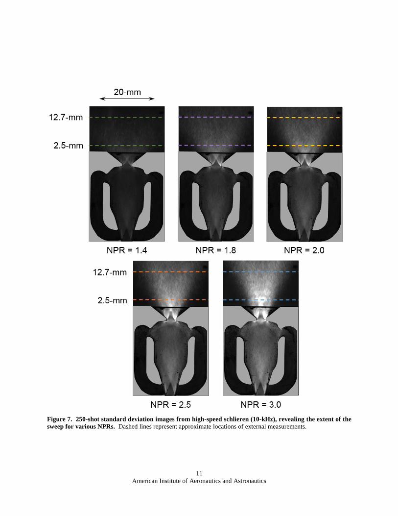
Figure 7 shows standard deviation images of the sweeping jet operating at different NPRs (which indicate, at
each pixel location, the standard deviation of the schlieren intensity based on 250 single-shots acquired at 10 kHz).
The dashed colored lines indicate the location of the first two external measurements relative to the nozzle exit.
Figure 7 prominently showcases the aforementioned shear layer features, whose intensity increases as the pressure
ratio increases. Also, the extent of the jet’s external sweep is shown in these images, narrowing as the pressure ratio
increases. Furthermore, no new flow features appear as the pressure ratio is increased, further emphasizing that the
qualitative structure of the internal flow is independent of pressure ratio.
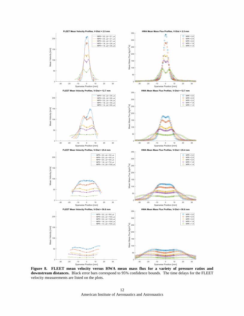
Figures 8 and 9 contain the mean and fluctuation profiles, respectively, of the external flow field as measured by
FLEET and HWA for different downstream distances and pressure ratios (for sample single-shot profiles, see Figure
14 in the Appendix). The fluctuation profiles were obtained by computing the root mean square (RMS) of the
mean-subtracted velocity fluctuations. The FLEET data were based on over 2,400 single-shot measurements while
hot-wire data were based on over 400,000 samples for each spanwise location. Note that excessively noisy FLEET
data obtained at the ends of the probed region were excluded from the plots, explaining why the profiles do not span
the entire abscissa. Data with excessive noise were identified by a loss of precision in the velocity fluctuation
profiles—the measured value of fluctuations would ‘diverge’ from the values in the center of the jet, increasing two-
to fivefold depending on the pressure ratio. Data after the point of divergence were excluded from both the
fluctuating and mean profiles. The loss of precision was attributed primarily to the relatively low laser fluence and
is discussed in more detail in the Appendix.
Several general trends of sweeping jet actuators can be identified in the mean profiles of Figure 8. One such
trend is that as the pressure ratio increases, the velocity increases, as expected, but the sweep angle decreases. This
reduction in sweep angle with increasing pressure ratio, which is qualitatively depicted in Figure 7, has been
observed in other studies and is undesirable because the size of the region of influence of the sweeping jet is
diminished.6 Another trend is that as the jet travels downstream, it loses velocity and broadens (consistent with PIV
data).3,5 These trends are expected for sweeping jets and even steady, axisymmetric jets, since the jet flow
decelerates and spreads out as it transfers momentum to the quiescent surroundings. A documented feature of
sweeping jets is that the rates of spreading and velocity decay are faster than a comparable steady, axisymmetric,
turbulent jet.3,5 Based on the HWA results, our sweeping jet exhibited a spreading rate, d𝑦1/2/d𝑥, of 0.5 to 1.2,
substantially larger than the spreading rate of about 0.1 for steady turbulent jets.25 The spreading rate for the SWJ
increased as pressure ratio decreased. Note the jet half-width, 𝑦1/2, was defined as the average spanwise position for
which the mass flux decreased to one-half of its maximum value within the spanwise profile.
It should also be noted that although the mean velocities are less than the local speed of sound (≈320 m/s for an
isentropic expansion from the source at 𝑇0 = 308 K), the jet contains a significant number of instantaneous
velocities that are supersonic. This is evident in the FLEET velocity histograms of Figure 10 for NPRs of 2.5 and
3.0 at 2.5 mm downstream and by the presence of shock diamonds in the phase-averaged images of Figure 6.
Visually comparing FLEET to HWA, the spanwise profiles are, in general, qualitatively similar. One difference
is that the width of the jet was slightly broader for FLEET than HWA. This might be explained by 1) the
measurement locations being at different downstream distances during the two sets of testing since the tests were
performed in different laboratories and 2) the finite time delay of the FLEET measurements allows for spanwise
velocity components to effectively broaden the jet between the first and second exposures. Both effects were
estimated to be of similar order. Another difference is that the FLEET data measured an asymmetrical jet profile in
certain cases, particularly for 12.7 mm downstream at NPRs of 2.5 and 3.0. The jet may have been slightly
disturbed during the data acquisition period (which occurs over 2.4 s), causing the profile to be skewed. It is also
possible that jet and laser were partially phase-locked since they were operating at similar frequencies (near 1 kHz).
However, the phase-locking would not have been complete since the jet has prominent overtones at frequencies
other than its fundamental. There are also noticeable asymmetries in the data at 25.4 and 50.8 mm. This may have

American Institute of Aeronautics and Astronautics
8
been the result of the translation stage, which enabled the downstream distance to be varied, not translating perfectly
in the streamwise direction and causing the jet flow to be slanted.
It should also be mentioned that the HWA testing was not without its sources of uncertainty. During testing, the
stagnation temperature of the flow drifted as much as 5 K in some cases and was not accounted for in the
calibration. Also, for the higher-speed data, some of the mass fluxes substantially exceeded the instrument’s
calibration range and were coerced to the highest value on the calibration curve (which itself was an extrapolation
from the highest measured calibration point). This is evident by the peak around 520 kg/m2/s in the HWA mass flux
histograms for 2.5 mm downstream and NPRs of 2.5 and 3.0 (Figure 10).
The fluctuation quantities in Figure 9 are similar in magnitude to their counterpart mean quantities in Figure 8.
The ratio of fluctuation to mean quantities is significantly larger than that of a comparable steady, axisymmetric,
turbulent jet. This feature of SWJ actuators has been previously observed and is caused primarily by the sweeping
motion of the jet (i.e., for a given location, the jet is present for certain instances and absent for others, leading to
significant fluctuations with respect to time).5
Like the mean profiles, the fluctuation profiles are, in general, qualitatively similar for both FLEET and HWA.
Again, the FLEET fluctuation profiles possess an asymmetry that is not present in the hot-wire data, probably for the
same reasons mentioned above. Perhaps the most striking difference is that the FLEET fluctuation profiles exhibit
an offset: in the low velocity, ‘quiescent’ regions, the profiles decay to a finite value (e.g., ≈25 m/s for 2.5 mm
downstream) rather than zero. This offset is attributed to the precision of the FLEET measurement which varies
inversely with time delay26 (see the Appendix for measurements of the precision).
Figure 10 shows the histograms of the FLEET and HWA measurements at the center spanwise location of the
sweeping jet for 2.5 and 12.7 mm downstream for the five tested NPRs. The histograms at 25.4 and 50.8 mm were
omitted for the sake of brevity. The general trend is that the spread of data narrows and amasses toward the lower
values as downstream distance increases or pressure ratio decreases. This trend holds for 25.4 and 50.8 mm. The
right-most peaks around 520 kg/m2/s for 2.5 mm downstream at NPRs of 2.5 and 3.0 are a result of the hot-wire
probe measuring fluxes above its calibration range. The highest calibration point was 470 kg/m2/s and a third-order
polynomial permitted extrapolation to 520 kg/m2/s. As mentioned previously, values exceeding the upper bound of
extrapolation were coerced to 520 kg/m2/s. Conspicuous peaks for NPRs of 2.5 and 3.0 at 2.5 mm, along with
evidence of supersonic velocities (from FLEET), indicate that the hot-wire calibration should have been extended to
higher mass fluxes.
Regarding the FLEET data, there was substantial supersonic flow (≳ 320 m/s) for NPRs of 2.5 and 3.0 at 2.5
mm, but this supersonic contribution diminished quickly once the pressure ratio was lowered or the downstream
distance was increased. There were some supersonic velocities at 12.7 mm, but most of the velocities were subsonic
with a large grouping below 100 m/s.
Overall, the FLEET and HWA histograms were similar to one another and both flow quantities tended to
decrease as distance increased or pressure ratio decreased. Nevertheless, there are several specific differences worth
noting. First, the FLEET results appear nosier since they were computed from significantly fewer measurements
than HWA (2,400 versus 400,000). Second, there are relatively few results below 50 kg/m2/s for the hot-wire (i.e.,
an offset) whereas FLEET has measurements of zero velocity. This offset is most noticeable at 2.5 mm for NPRs of
2.5 and 3.0 and can be attributed to several factors. One factor, which plays only a small part, is that the hot-wire
suffers from reduced sensitivity, d(𝜌𝑢)/d𝑒, to low mass fluxes. Another factor, which plays a larger part, is that the
FLEET measurements (at 1 kHz) were inadvertently phased locked to the jet (oscillating at nearly 1 kHz for these
NPRs), leading to over sampling of the phases associated with lower velocity. The higher sampling rate of HWA
(102 kHz) is more immune to phase-locking errors. One possible solution would have been to lower the FLEET
data acquisition rate from its maximum of 1 kHz to, say, 10 Hz to achieve a more uniform sampling of the phases.
A third and similarly important factor is that the hot-wire probe primarily senses net mass fluxes perpendicular to
the axis of the wire whereas FLEET (in the present setup) only senses velocities in the streamwise direction.
Therefore, when the jet is away from the centerline and at an angle relative to the streamwise direction, it has larger
spanwise velocity components than streamwise ones and the hot-wire would tend to measure higher mass fluxes
(i.e., ‘velocities’) than FLEET which is insensitive to the spanwise components.
In general, FLEET is a direct measurement of velocity (resolving both magnitude and direction) for subsonic
through supersonic flows whereas HWA has a limited ability to measure velocity magnitude outside a very specific
range of flow regimes.

American Institute of Aeronautics and Astronautics
9
Figure 5. Schlieren single-shot (top) and 250-shot phase-averaged (bottom) images of sweeping jet actuator
at six phases of its oscillation cycle. Jet is operating with air at NPR = 1.4. Phases 1 through 6 correspond
approximately to 0.2𝜏, 0.3𝜏, 0.5𝜏, 0.7𝜏, 0.8𝜏, and 1.0𝜏, respectively, where 𝜏 is the SWJ’s period.

American Institute of Aeronautics and Astronautics
10
Figure 6. 250-shot phase-averaged images for various NPRs. Columns 1 through 6 correspond to the same
phases shown in Figures 1 and 5.
American Institute of Aeronautics and Astronautics
11
Figure 7. 250-shot standard deviation images from high-speed schlieren (10-kHz), revealing the extent of the
sweep for various NPRs. Dashed lines represent approximate locations of external measurements.
American Institute of Aeronautics and Astronautics
12
Figure 8. FLEET mean velocity versus HWA mean mass flux for a variety of pressure ratios and
downstream distances. Black error bars correspond to 95% confidence bounds. The time delays for the FLEET
velocity measurements are listed on the plots.

American Institute of Aeronautics and Astronautics
13
Figure 9. FLEET velocity fluctuations versus HWA mass flux fluctuations for a variety of pressure ratios
and downstream distances.

American Institute of Aeronautics and Astronautics
14
Figure 10. Histograms of centerline FLEET velocities versus HWA mass fluxes for a variety of pressure
ratios and downstream distances. For sake of brevity, data at 25.4 and 50.8 mm were omitted.
B. Internal Flow Field - FLEET
Figure 11 shows the mean streamlines, mean velocities and RMS of velocity fluctuations for an initial spot
location of (𝑥, 𝑦) = (−6.2 mm, 0.2 mm) at the five pressure ratios. Note that these data are presented with the SWJ
oriented as shown in Figure 4, where the red box approximately demarcates the measurement domain. Data for 𝑥 >−3.3 mm were not reported because strain and break-up of the tagged region rendered the measurements unusable.
It should also be noted that these plots are not true Eulerian velocity maps (as is commonly outputted by
computational fluid dynamics) since they were created by tracking the advection of a single tagged region a number
of times. The measurement is analogous to injecting dye into a liquid flow at a point to visualize the flow field, but
more quantitative. Also note that these results could be compared to a computer simulation with Lagrangian particle
tracking and filtering for only those particles that pass through the initial spot location.

American Institute of Aeronautics and Astronautics
15
Inspecting Figure 11, the mean streamlines show that the flow is predominantly along the streamwise direction
with some turning upstream of the throat (which is located at 𝑥 = −4.0 mm). The turning indicates that some of the
flow is entering the feedback loops.
The mean velocity plot shows a positive velocity gradient in the streamwise direction and depressed velocities
off of the centerline axis. The gradient is expected since this region of the actuator acts as a converging nozzle.
Significant acceleration downstream of the throat for NPR ≥ 2.0 confirms the presence of choked flow (i.e., sonic at
throat) since the flow continues to accelerate as it travels through the diverging diffuser.
The largest velocity fluctuations are localized to the region downstream of the throat (most conspicuously for
NPRs 2.5 and 3.0). These velocity fluctuations are roughly 40% to 60% of the values found in the external flow for
the corresponding NPRs at 2.5 mm downstream (cf. Figure 9). This has several possible explanations: 1) the
favorable pressure gradient in this region acts to suppress velocity fluctuations, 2) the measured velocities are
spatially filtered such that the streakline must pass through the initial spot location, therefore, not all velocities (and
velocity fluctuations) are included in this map, 3) there are no shocks in this region (unlike the external jet which has
shock diamonds at NPR ≥ 2.5) which tend to amplify turbulent fluctuations27 and 4) the precision of the internal
measurement is likely better than the external measurement due to the improved SNR associated with the relatively
high laser fluence and use of pure nitrogen.
Note that the gradients of mean velocity and velocity fluctuation both increase as NPR increases, with the mean
velocity gradient having the more prominent increase.
Figure 11. FLEET measurements of internal flow field. Throat and centerline were at positions of 𝑥 =−4.0 mm and 𝑦 = −0.2 mm, respectively. The spot’s origin was around (𝑥, 𝑦) = (−6.2 mm, 0.2 mm).
NPR
3.0
2.5
2.0
1.8
1.4

American Institute of Aeronautics and Astronautics
16
Figure 12 plots the mean velocity along the centerline axis to illustrate the dependence of acceleration on the
nozzle pressure ratio. The error bars denote one standard deviation of velocity and indicate the magnitude of the
fluctuations. Based on the plot, there was no evidence of a strong normal shockwave inside the actuator since a
precipitous velocity decrease was absent. A strong shock was also noticeably absent from the schlieren images.
(There was initially some speculation that a shock might be present and causing the observed narrowing of the
sweep angle with increasing pressure ratio.) Furthermore, the plot illustrates presence of supersonic flow for NPR ≥
2.0 since the sum of the mean and standard deviation exceeds the local speed of sound (≈310 m/s for isentropic
expansion from 𝑇0 ≈ 294 K), corroborating statements above about NPR ≥ 2.0 exhibiting choked flow. In
particular, NPRs of 2.5 and 3.0 experience ‘mostly continuous’ choking and NPR of 2.0 experiences ‘intermittent’
choking. This is supported by the external velocity histograms in Figure 10 which display noteworthy supersonic
contributions for NPR ≥ 2.0. A pressure ratio of 1.8, just below the necessary isentropic value of 1.89, seems to be
on the cusp of choking, but not yet choking; any apparent supersonic velocities in its histogram are likely an artifact
of measurement precision rather than intermittent choking.
Figure 12. Mean centerline velocities from internal measurements. Error bars denote one standard deviation.
C. Concentration in the External Flow Field - FLEET
Figure 13 shows the mean profiles (based on 1,200 single-shot images) of relative oxygen mole fraction as
estimated from changes in FLEET signal intensity obtained 75 ns after the laser pulse. A relative mole fraction of
zero corresponds to pure nitrogen whereas a mole fraction of one corresponds to air. Mixing is gauged by noting the
jet’s relative mole fraction evolution from zero to values approaching one. The profiles are grouped by pressure
ratio with each curve denoting a different distance downstream of the exit. There were no discernable changes in
signal intensity beyond 25.4 mm for pressure ratios of 1.4 and 1.8; therefore, data at 50.8 mm were not reported.
Note that these results have not been corrected for the signal variation that occurs due to the compressibility of
the gas; experiments have shown that FLEET signal intensity depends linearly on gas density.28 Therefore, these
plots are primarily proof-of-concept, qualitative estimates of mole fraction that showcase an added benefit of
FLEET-based measurements. Nevertheless, there are potential ways of decoupling the influence of density on the
concentration measurements. One such way is to take measurements of the SWJ running air instead of nitrogen as a
type of calibration. The resulting mean profiles would contain only the effects of density and spatial variation of
laser fluence since the concentration of oxygen would be fixed. Then, concentration measurements with the SWJ
running compressed nitrogen could be taken. Dividing the nitrogen (data) curves by the air (calibration) curves
should isolate the effect of concentration on signal intensity and therefore yield an accurate mean measurement of
oxygen concentration. A second option is to measure the Rayleigh scattering from the femtosecond laser pulse since
Rayleigh scattering is proportional to gas density. This would have the advantage of allowing for single-shot
density measurements in addition to time-averaged ones.

American Institute of Aeronautics and Astronautics
17
Neglecting the effect of variable density, these plots convey that the jet becomes well mixed (i.e., oxygen mole
fraction increases to within a few percent of the ambient value) within 12.7 mm or roughly four throat diameters
downstream of the exit and fully mixed (i.e., oxygen mole fraction asymptotes to within a few tenths of a percent of
the background level of oxygen in the vicinity of the SWJ outlet) within 25.4 mm or roughly eight throat diameters.
These changes in signal intensity would be difficult to attribute primarily to density since it did not change by a
factor of 7 to 14 (which was the observed change in signal intensity). The dip in the center of the curves for
pressure ratios of 2.0 and above is probably the combined result of density variation and the reduced mixing
associated with lower velocity fluctuations (cf. dips in velocity fluctuations in Figure 9).
The lack of overlap for the wings of some of the curves was caused by the baseline calibration in air being taken
without the jet running and with slightly different camera settings (unavoidable because of experimental
difficulties). The inconsistencies in the wings should be given marginal weighting since, at the very least, density
was not decoupled and a proper baseline calibration was not obtained. The overall trend of rapid mixing should be
accepted as reasonably valid since there were no other known sources which could account for the factor of 7 to 14
change in signal.
Although velocity measurements were made simultaneously with the concentration measurements, they are not
reported herein. The simultaneous velocity measurements, made when operating the camera/intensifier in a frame-
straddling mode, were excessively noisy because of difficultly in precisely discriminating the displaced line from an
un-displaced ghosting artifact. The ghosting problem occurred when framing the camera at 40 kHz; if the falling
edge of the first intensifier gate was very close to the end of the first camera exposure (necessary for achieving short
time delays), up to 40% of the signal would bleed into the next frame.

American Institute of Aeronautics and Astronautics
18
Figure 13. Profiles of relative oxygen mole fraction based on FLEET signal intensity for different pressure
ratios and downstream distances. Black error bars denote 95% confidence bounds.
D. Comparison of FLEET Velocimetry and Hot-Wire Anemometry
Since both FLEET and HWA were utilized in this experimental investigation, it is worth discussing how FLEET
velocimetry compares to more traditional, single hot-wire anemometry.
Strengths of FLEET relative to HWA:
o Instantaneous line (or point) measurements of FLEET with every data capture; single-shot spatial
cross-correlations and velocity profiles (via line measurements)
o Faster data acquisition since no traversing is needed to obtain spatial profiles
o Larger dynamic range of measurement (subsonic to supersonic, discriminate negative velocities)
o Nonintrusive, tolerant of tight spatial constraints since laser-based: able to make measurements
inside the actuator

American Institute of Aeronautics and Astronautics
19
o Simpler calibration since only ruler/dot-card is needed in contrast to calibration wind tunnel
Weaknesses of FLEET relative to HWA:
o More computationally intensive image processing rather than polynomial lookup
o Optical access required since laser-based
o Optics in path of laser beam must be compatible with femtosecond duration laser pulses
o Significantly more expensive acquisition system (laser, camera and intensifier)
The relatively poor precisions measured during post-SWJ testing were not listed as a weakness since they were
not inherent to the technique, but rather the result of the particular experimental setup (which employed low laser
fluences). Use of higher laser fluences can yield precisions in air of better than a few meters per second.26,28
IV. Conclusion
FLEET velocimetry was successfully demonstrated in a highly unsteady, oscillatory flow containing subsonic,
transonic, and supersonic velocities. Measurements were made in the external flow field with FLEET and single
hot-wire anemometry (for qualitative comparison). Measurements of the internal flow field inside the actuator were
made with FLEET alone. High-speed and phase-averaged schlieren provided visualization of both external and
internal flows.
The external FLEET velocity profiles were, in general, qualitatively similar to the mass flux profiles measured
by HWA; however, two potential drawbacks were noted. 1) Phase-locking may have been occurring between the
FLEET measurement (acquiring at 1 kHz) and the sweeping jet (with a dominant frequency around 1 kHz) possibly
explaining the reason for asymmetric jet profiles which were not observed in the HWA results. 2) FLEET suffered
from noticeably worse precision (≲ 25 m/s) than HWA, attributable to the relatively low laser fluences utilized in
the experiment. The low laser fluence was a consequence of writing a long line (to simplify data acquisition) and
trying to avoid perturbing the flow via energy deposition. Unfortunately, this low laser fluence ultimately resulted
in degraded measurement precision. Previous experiments have reported precisions of a few meters per second in
air and less than one meter per second in nitrogen when operating at higher laser fluences; therefore, the low
precision was a result of the chosen experimental setup, not a fundamental limitation of the technique. In general,
FLEET demonstrated better overall dynamic range and improved sensitivity to low velocities, in addition to
explicitly measuring velocity in the compressible flow regime.
The expected trends in the external profile of the sweeping jet were observed such as an increasing jet velocity
(desirable) and decreasing sweep angle (undesirable) with increasing pressure ratio. Furthermore, the jet had
significant spreading and velocity decay rates as expected.
FLEET provided measurements of the internal flow field which were inaccessible to probe-based methods and
would have been difficult to perform with certain other non-intrusive methods. The velocity and fluctuation
gradients within the device were mapped out and indicated that choked flow was achieved for pressure ratios greater
than or equal to 2.0. Also, there was no evidence of a shockwave (sudden decrease in velocity) inside the device
during operation.
Qualitative mixing measurements were demonstrated as a proof-of-concept. This is a potential added-benefit of
FLEET velocimetry. The measurements were based on the signal intensity variation of FLEET with oxygen
concentration and were primarily qualitative since there was no correction for the density change resulting from
compressibility. A method was described to correct for the density variation in future work. The mixing
measurements conveyed that the jet became well mixed within 12.7 mm downstream (or roughly four throat
diameters downstream) and fully mixed within 25.4 mm (or roughly eight throat diameters).
The high-speed and especially the phase-averaged schlieren images demonstrated that the general character of
the internal flow is largely independent of pressure ratio—no new flow structures arise (other than changes to the
magnitude of gradients or features). The structure of the external flow evolves with pressure ratio in the sense that
the sweep angle decreases and shock diamonds appear.
Appendix
A. Single-Shot Velocity Measurements
Figure 14 shows a sampling of the FLEET single-shot (i.e., instantaneous) velocity profiles in the external flow
field for NPRs of 1.4 and 3.0 at 2.5 mm downstream of the exit. Compared to the mean profiles, the single-shots are
nosier and have finite negative velocities (both of which are artifacts of the line-fitting imprecision associated with
low SNR, discussed in the following section).

American Institute of Aeronautics and Astronautics
20
Figure 14. FLEET single-shot and mean velocity profiles for two NPRs (in air) at 2.5 mm downstream.
B. Precision of FLEET Velocimetry
At the conclusion of the sweeping jet tests, the precision of the FLEET setup was characterized (Figure 15) by
measuring the velocity of quiescent air using the same laser and camera settings as the sweeping jet tests. As
expected, the precision improved with time delay. Table 1 compares these post-test precisions to the estimated
precisions of the sweeping jet measurements (based on the RMS value in the quiescent regions) and the precisions
reported by Ref. 26 for a similar camera/intensifier setup, but at higher laser fluence. Measurement precision is
proportional to SNR which itself is proportional to the laser fluence for these focal lengths. Accordingly, the
precision improves three- to fourfold when laser fluence is raised sevenfold. This suggests the lower precision of
FLEET as compared to HWA is not a fundamental limitation of the technique, but rather that of the experimental
setup and could be remedied with tighter focusing or use of a higher power laser. Therefore, an alternative approach
might have been to focus more tightly (with a shorter line) and pan the field of view, although this may have led to
new experimental uncertainties (such as those associated with stitching fields of view together). Note there were
additional sources of imprecision such as facility vibration or beam pointing, since the reference and delay images
are not recorded sequentially.
Figure 15. Post-SWJ testing measurement of FLEET precision in quiescent air (1-m FL, 2.0 mJ).
Table 1. Precision comparison of FLEET in air using intensified CMOS cameras (20 µm pixels).

American Institute of Aeronautics and Astronautics
21
SWJ Testing, Estimated RMS in Jet (1-m FL, 2.0 mJ)
[m/s]
Time Delay (1-µs gate)
[µs]
25 2.1
20 3.6
10 10.6
Post-SWJ Testing, RMS in Quiescent Air (1-m FL, 2.0 mJ)
[m/s]
Time Delay (1-µs gate)
[µs]
34 2.0
24 3.0
19 4.0
10 10.1
Ref. 26, ≈RMS in Quiescent Air (500-mm FL, 3.0 mJ)
[m/s]
Time Delay (2-µs gate)
[µs]
3.2 8.3
2.4 16.7
C. Data Point Density of Internal FLEET Measurements
Figure 16 shows the distribution of data points (velocities and corresponding positions) on the uniform grid.
Note the grid size varies slightly among the different plots. The greatest density of data points is near the origin of
the FLEET spot at (−6.2 mm, 0.2 mm) and decreases with progressing distance downstream.
Figure 16. Number of data points within each grid position used for producing mean and RMS values.
3.0
2.5
2.0
1.8
1.4
NPR

American Institute of Aeronautics and Astronautics
22
Acknowledgments
C. J. Peters was supported by a NASA Space Technology Research Fellowship. S. B. Jones was the technician
at NASA Langley and his help was greatly appreciated. P. M. Danehy and R. A. Burns were supported by the
NASA Langley Research Center’s IRAD Program. B. F. Bathel was supported by the Aerodynamic Evaluation and
Test Capabilities (AETC) project. The authors wish to thank J. A. Inman for assistance in reviewing the manuscript.
Note that NASA does not endorse any particular manufacturer of equipment used in this paper. The names of the
manufacturers are included for clarity and the equipment tested was mainly chosen because of its availability.
Equipment from other manufacturers may perform equally as well or better.
References
1Raghu, S., “Fluidic oscillators for flow control,” Experiments in Fluids, Vol. 54, No. 2, pp. 1-11, 2013. 2Bobusch, B. C., Woszidlo, R., Bergada, J. M., Nayeri, C. N., Paschereit, C. O., “Experimental study of the internal flow
structures inside a fluidic oscillator,” Experiments in Fluids, Vol. 54, No. 6, pp. 1-12, 2013 3Gärtlein, S., Woszidlo, R., Ostermann, F., Nayeri, C. N., and Paschereit, C. O., “The Time-Resolved Internal and External
Flow Field Properties of a Fluidic Oscillator” in 52nd Aerospace Sciences Meeting, National Harbor, Maryland, 2014. 4Bobusch, B. C., Woszidlo, R., Krüger, O., Paschereit, C. O., “Numerical Investigations on Geometric Parameters Affecting
the Oscillation Properties of a Fluidic Oscillator” in 21st AIAA Computational Fluid Dynamics Conference, San Diego,
California, 2013. 5Koklu, M., and Melton, L., “Sweeping Jet Actuator in a Quiescent Environment” in 43rd AIAA Fluid Dynamics Conference,
San Diego, California, 2013. 6Seele, R., Graff, E., Lin, J., Wygnanski, I., “Performance Enhancement of a Vertical Tail Model with Sweeping Jet
Actuators” in 51st AIAA Aerospace Sciences Meeting including the New Horizons Forum and Aerospace Exposition, Grapevine,
Texas, 2013 7Northon, K., Ed., “NASA, Boeing Finish Tests of 757 Vertical Tail With Advanced Technology,” NASA Press Release 13-
340, 2013. 8Milholen, W. E., Jones, G. S., Chan, D. T., Goodliff, S. L., Anders, S. G., Melton, L. P., Carter, M. B., Allan, B. G., and
Capone, F. J., “Enhancements to the FAST-MAC Circulation Control Model and Recent High-Reynolds Number Testing in the
National Transonic Facility” in 31st AIAA Applied Aerodynamics Conference, San Diego, California, 2013. 9Jones, G. S., Milholen, W. E., Fell, J. S., Webb, S. R., Cagle, C. M., “Using Computational Fluid Dynamics and
Experiments to Design Sweeping Jets for High Reynolds Number Cruise Configurations” in 8th AIAA Flow Control Conference,
Washington, D.C., 2016. 10Gokoglu, S. A., Kuczmarski, M. A., Culley, D. E., Raghu, S., “Numerical Studies of a Supersonic Fluidic Diverter Actuator
for Flow Control,” in 5th Flow Control Conference, Chicago, Illinois, 2010. 11Hirsch, D., Graff, E. C., Gharib, M., “Compressible Flows in Fluidic Oscillators,” APS Division of Fluid Dynamics: Gallery
of Fluid Motion [available online], 2013. 12Krüger, O., Bobusch, B. C., Woszidlo, R., Paschereit, C. O., “Numerical Modeling and Validation of the Flow in a Fluidic
Oscillator,” in 21st AIAA Computational Fluid Dynamics Conference, San Diego, California, 2013. 13Edwards, M., Limbach, C., Miles, R., and Tropina, A., “Limitations on High-Spatial Resolution Measurements of
Turbulence Using Femtosecond Laser Tagging” in 53rd AIAA Aerospace Sciences Meeting, Kissimmee, Florida, 2015. 14Burns, R. A., Peters, C. J., Danehy, P. M., “Femtosecond-Laser-Based Measurements of Velocity and Density in the NASA
Langley 0.3-m Transonic Cryogenic Tunnel” in 32nd AIAA Aerodynamic Measurement Technology and Ground Testing
Conference, Washington, D.C., 2016. 15Calvert, N., Dogariu, A., and Miles, R., “FLEET Boundary Layer Velocity Profile Measurements” in 44th AIAA
Plasmadynamics and Lasers Conference, San Diego, California, 2013. 16Miles, R., Edwards, M., Michael, J., Calvert, N., and Dogariu, A., “Femtosecond Laser Electronic Excitation Tagging
(FLEET) for Imaging Flow Structure in Unseeded Hot or Cold Air or Nitrogen” in 51st AIAA Aerospace Sciences Meeting
including the New Horizons Forum and Aerospace Exposition, Grapevine, Texas, 2013. 17Michael, J., Edwards, M., Dogariu, A., and Miles, R., “Femtosecond laser electronic excitation tagging for quantitative
velocity imaging in air,” Applied Optics, Vol. 50, No. 26, pp. 5158-5162, 2011. 18Edwards, M. “Femtosecond Laser Electronic Excitation Tagging,” Undergraduate Senior Thesis, Princeton University,
2012. 19DeLuca, N., Miles, R., Kulatilaka, W., Jiang, N., and Gord, J., “Femtosecond Laser Electronic Excitation Tagging (FLEET)
Fundamental Pulse Energy and Spectral Response” in 30th AIAA Aerodynamic Measurement Technology and Ground Testing
Conference, Atlanta, Georgia, 2014. 20Halls, B. R., Jiang, N., Gord, J. R., Danehy, P. M., Roy, S., “Mixture-Fraction Measurements with Femtosecond-Laser
Electronic-Excitation Tagging,” submitted to Optics Letters. 21Raman, G., Raghu, S., “Cavity Resonance Suppression Using Miniature Fluidic Oscillators,” AIAA Journal, Vol. 42, No.
12, pp. 2608-2611, 2004.

American Institute of Aeronautics and Astronautics
23
22Vasta, V. N., Koklu, M., Wygnanski, I. L., Fares, E., “Numerical Simulation of Fluidic Actuators for Flow Control
Applications” in 6th AIAA Flow Control Conference, New Orleans, Louisiana, 2012. 23Kovásznay, L. S. G, “The Hot-Wire Anemometer in Supersonic Flow,” Journal of the Aeronautical Sciences, Vol. 17, No.
9, pp. 565-572, 1950. 24Willert, C. E., Mitchell, D. M., Soria, J., “An assessment of high-power light-emitting diodes for high frame rate schlieren
imaging,” Experiments in Fluids, Vol. 53, No. 2, pp. 413-421, 2012. 25Pope, S. B., Turbulent Flows, 1st ed., Cambridge University Press, New York, Chap. 5, pp. 101,139, 2011. 26Peters, C. J., Danehy, P. M., Bathel, B. F., Jiang, N., Calvert, N. D., Miles, R. B., “Precision of FLEET Velocimetry using
High-Speed CMOS Camera Systems” in 31st AIAA Aerodynamic Measurement Technology and Ground Testing Conference,
Dallas, Texas, 2015. 27Andreopoulos, Y., Agui, J. H., Briassulis, G., “Shock Wave–Turbulence Interactions,” Annual Review of Fluid Mechanics,
Vol. 32, pp. 309-345, 2000. 28Burns, R. A., Danehy, P. M., Halls, B. R., Jiang, N., “Application of FLEET Velocimetry in the NASA Langley 0.3-meter
Transonic Cryogenic Tunnel,” in 31st AIAA Aerodynamic Measurement Technology and Ground Testing Conference, Dallas,
Texas, 2015.