feminis
TRANSCRIPT
8/15/2019 Feminis
http://slidepdf.com/reader/full/feminis 1/82
UNIVERSITA’ CATTOLICA DEL SACRO CUORE
WORKING P APER
DISCEDipartimenti e Istituti di Scienze Economiche
FROM SIMPLE GROWTH TO NUMERICAL SIMULATIONS: A PRIMER IN
DYNAMIC PROGRAMMING
Gianluca Femminis
ITEMQ 45 - Settembre - 2007

8/15/2019 Feminis
http://slidepdf.com/reader/full/feminis 2/82
QUADERNI DELL’ISTITUTO DI
TEORIA ECONOMICA E METODI QUANTITATIVI
FROM SIMPLE GROWTH TO NUMERICAL SIMULATIONS: A PRIMER IN
DYNAMIC PROGRAMMING
Gianluca Femminis
Quaderno n. 45 / settembre 2007
U NIVERSITÀ CATTOLICA DEL SACRO CUORE MILANO

8/15/2019 Feminis
http://slidepdf.com/reader/full/feminis 3/82
ISTITUTO DI TEORIA ECONOMICA E METODI QUANTITATIVI (ITEMQ)
Membri Comitato di Redazione
Luciano Boggio Luciano BoggioLuigi Filippini Luigi FilippiniLuigi Lodovico Pasinetti Luigi Lodovico Pasinetti
Paolo Varri ( Direttore) Paolo VarriDomenico Delli GattiDaniela ParisiEnrico BellinoFerdinando ColomboGianluca FemminisMarco Lossani
I Quaderni dell’Istituto di Teoria Economica e Metodi Quantitativi possono essere richiesti a:
The Working Paper series of Istituto di Teoria
Economica e Metodi Quantitativi can be requested at:
Segreteria ITEMQUniversità Cattolica del S. Cuore
Via Necchi 5 - 20123 MilanoTel. 02/7234.2918 - Fax 02/7234.2923
E-mail [email protected]
8/15/2019 Feminis
http://slidepdf.com/reader/full/feminis 4/82
Finito di stampare nel mese di settembre presso la Redazione stampati
Università Cattolica del Sacro Cuore
Il Comitato di Redazione si incarica di ottemperare agli obblighi previsti
dall’art. 1 del DLL 31.8.1945, n. 660 e successive modifiche
“ESEMPLARE FUORI COMMERCIO PER IL DEPOSITO LEGALE AGLI EFFETTI DELLA LEGGE 15APRILE 2004, N. 106”
8/15/2019 Feminis
http://slidepdf.com/reader/full/feminis 5/82
FROM SIMPLE GROWTH TO NUMERICAL
SIMULATIONS: A PRIMER IN DYNAMIC
PROGRAMMING
GIANLUCA FEMMINIS
Abstract. These notes provide an intuitive introduction to dynamicprogramming. The …rst two Sections present the standard deterministicRamsey model using the Lagrangian approach. These can be skippedby whom is already acquainted with this framework. Section 3 showshow to solve the well understood Ramsey model by means of a Bellman
equation, while Section 4 shows how to “guess” the solution (when this ispossible). Section 5 is devoted to applications of the envelope theorem.Section 6 provides a “paper and pencil” introduction to the numericaltechniques used in dynamic programming, and can be skipped by theuninterested reader. Sections 7 to 9 are devoted to stochastic modelling,and to stochastic Bellman equations. Section 10 extends the discussionof numerical techniques. An Appendix provides details about the Mat-lab routines used to solve the examples.
Date : August 30, 2007Keywords: Dynamic programming, Bellman equation, Optimal growth, Numerical tech-niques.JEL Classi…cation: C61, O41, C63.Correspondence to: Gianluca Femminis, Università Cattolica, Largo Gemelli 1, 20123Milano, Italy; e-mail address : [email protected]: I wish to thank Marco Cozzi for helpful comments and detailed
suggestions.1

8/15/2019 Feminis
http://slidepdf.com/reader/full/feminis 6/82
2 GIANLUCA FEMMINIS
1. Utility maximization in a finite-horizon deterministic setting
One of the ingredients that we …nd in almost any growth model is theanalysis of the agent’s consumption behavior. In fact consumption, through
savings, determines capital accumulation, which, in turn is one of the key
“engines of growth”. In this Section, we consider the problem of the optimal
determination of consumption in the easiest possible framework, in which the
lifetime of a single consumer is of a …nite and known length. We solve this
intertemporal problem using the Lagrangian approach: once the problem is
well understood, it shall be easy to consider its in…nite horizon counterpart
and then to solve it by means of the dynamic programming approach. This
shall be done in Sections 2 and 3, respectively.
1.1. The problem. In our settings, a single consumer aims at maximizing
her utility over her …nite lifetime (hence, the consumer’s horizon is …nite).
Time is “discrete”, i.e., it is divided into periods of …xed length (say, a year
or a quarter), and our consumer is allowed to decide her consumption level
only once per period. The consumption goods she enjoys are produced by
means of a “neoclassical” production function.1
We suppose that our consumer optimizes from time 0 onwards, and that
her preferences are summarized by the following intertemporal utility func-tion:
(1.1) W 0 =T X
t=0
tU (ct);
where 2 (0; 1) is the subjective discount parameter, ct is consumption at
time t, and T + 1 is the length (in periods) of our consumer’s lifetime. As
for the single period utility function, U (ct); we accept the standard “neo-
classical” assumptions, requiring that, in every period, the marginal utility
is positive but decreasing, i.e. that U 0
(ct) > 0; and U
00
(ct) < 0: Moreover,we assume that: limct!0 U 0(ct) = 1:
1An analysis concerning a single consumer may seem very limited. In particular, as it willbecome clear in a while, a single agent–being alone–optimizes under the constraint of theproduction function. This appears to be in sharp contrast with what happens in the realworld. In fact, in a market economy, any optimizing consumer takes account of prices,wages, interest rates...However, it can be shown that if markets are competitive and agents are all alike, theresources allocation in our exercises is equivalent to the allocation or resources that isachieved by a decentralized economy. Hence, while our if is a rather big one, our analysis
is less limited than what it might seem at …rst sight.

8/15/2019 Feminis
http://slidepdf.com/reader/full/feminis 7/82
DYNAMIC PROGRAMMING: A PRIMER 3
Output (yt) is obtained by means of a production function, the argument
of which is capital (kt): 2
(1.2) yt = f (kt):
As any well-behaved “neoclassical” production function, Eq. (1.2) satis-
…es some conditions, that are:
a: f 0(kt) > 0;
b: f 00(kt) < 0;
(in words, the marginal productivity of capital is positive, but decreasing),
c: f (0) = 0;
(this means that capital is essential in production).
d: f 0(0) > + 1= 1;
e: limkt!1
f 0(kt) = 0;
(as it will become clear in what follows, hypotesis (d) implies that capital
at least at its lowest level is productive enough to provide the incentive
for building a capital stock, while assumptions (e) rules out the possibility
that capital accumulation goes on forever.) 3
At this point, it is commonly assumed that output can be either consumed
or invested, i.e. that yt = ct + it (which implies that we are assuming away
government expenditure). When capital depreciates at a constant rate, ;
the stock of capital owned by our agent in period 1 is: k1 = i0 + (1 )k0:
Accordingly, Eq. (1.2) and the output identity, yt = ct + it, imply that k1
can be written as:
k1 = f (k0) + (1 )k0 c0:
Hence, in general, we have that
(1.3) kt+1 = f (kt) + (1 )kt ct;
2If you feel disturbed by the fact that capital is the unique productive input, considerthat we can easily encompass a …xed supply of labour in our framework. We might havespeci…ed our production function as yt = g(kt; l), where l is the labour …xed supply; in thiscase we could have normalized l to unity and then we could have written f (kt) g(kt; 1):An alternative, and more sophisticated, way of justifying Eq. (1.2) is to assume that outputis obtained by means of a production function which is homogeneous of degree one, sothat there are constant returns to scale. Then, one interprets kt as the capital/labourratio.3What is really necessary is to accept that limkt!1 f 0(kt) < ; an hypothesis that canhardly b e considered restrictive. The assumption in the main text allows for a slightly
easier exposition.

8/15/2019 Feminis
http://slidepdf.com/reader/full/feminis 8/82
4 GIANLUCA FEMMINIS
for t = 0; 1; ::: ; T: In addition to the above set of dynamic constraints, we
require that
(1.4) kT +1 0:
In words, this obliges our consumer to end her life with a non-negative
stock of wealth. This condition must obviously be ful…lled by a consumer
which lives “in insulation” (a negative level of capital stock does not make
any sense in this case); if our agent is settled in an economic system where
…nancial markets are operative, what we rule out is the possibility that our
consumer dies in debt.
Summing up, we wish to solve the problem:
max W 0 = maxT X
t=0
tU (ct);
under the T constraints of the (1.3)-type and under constraint (1.4). No-
tice that the solution of the problem requires the determination of T + 1
consumption levels (c0; c1;::::;cT ), and of T + 1 values for the capital stock
(k1; k2;::::;kT +1).
We can approach the consumer’s intertemporal problem by forming a
“present value” Lagrangian:
L0 = U (c0) + U (c1) + 2U (c2) + ::: + T U (cT )
0[k1 f (k0) (1 )k0 + c0]
1[k2 f (k1) (1 )k1 + c1]
:::(1.5)
T 1T 1[kT f (kT 1) (1 )kT 1 + cT 1]
T T [kT +1 f (kT ) (1 )kT + cT ]
+ T kT +1:
To solve the problem, we must di¤erentiate (1.5) with respect to ct, kt+1,
t (for t = 0; 1;:::;T ); and with respect to :4
The …rst order conditions with respect to the T + 1 consumption levels
are:
4The condition we imposed on the single period utility function and on the productionfunction guarantee that we obtain a global maximum. See, e.g. Beavis and Dobbs [1990],
or de la Fluente [2000].

8/15/2019 Feminis
http://slidepdf.com/reader/full/feminis 9/82
DYNAMIC PROGRAMMING: A PRIMER 5
U 0
(c0) = 0
U 0(c1) = 1
::: = :::(1.6)
U 0(ct) = t
::: = :::
U 0(cT ) = T :
Notice that each Lagrange multiplier t expresses the consumer’s marginal
utility of consumption, as perceived in the future period t.
When our agent optimizes with respect to the T + 1 capital levels (fromk1 to kT +1), she obtains:
0 = 1[f 0(k1) + (1 )]
1 = 22[f 0(k2) + (1 )]
::::::
tt = t+1t+1[f 0(kt+1) + (1 )](1.7)
::::::
T
1T 1 = T T [f 0
(kT ) + (1 )]
T = T T :
Of course, derivation of (1.5) with respect to the Lagrange multipliers
t; t = 0; 1; 2;:::;T yields the set of constraints (1.3). Finally, derivation
of (1.5) with respect to gives the constraint (1.4); in addition one must
consider the “complementary slackness” condition:
(1.8) T kT +1 = 0 and 0;
which shall be commented upon in a while.
1.2. The Euler equation. Consider now any …rst order condition belong-
ing to group (1.7): one immediately sees that those equations can be ma-
nipulated using the appropriate …rst order conditions of group (1.6). The
typical result of a practice of this kind is:
(1.9) U 0
(ct) = U 0
(ct+1)[f 0
(kt+1) + (1 )]

8/15/2019 Feminis
http://slidepdf.com/reader/full/feminis 10/82
6 GIANLUCA FEMMINIS
This condition is known as the Euler equation, which is of remarkable
importance not only to understand many growth models but also in con-
sumption theory.
The Euler equation (1.9) tells us that an optimal consumption path must
be such that – in any period – the marginal utility for consumption is equal
to the following period marginal utility, discounted by and capitalized by
means of the net marginal productivity of capital. To gain some intuition
about the economic meaning of Eq. (1.9), consider that it can be interpreted
as prescribing the equality between the marginal rate of substitution between
period t and period t + 1 consumptions (i.e. U 0(ct)=U 0(ct+1)); and the
marginal rate of transformation, f 0(kt+1) + (1 ):5
To improve your understanding of this point, pick a consumption level forperiod t, say ~ct; then choose a consumption level for the subsequent period
t+1; say ~ct+1.6 Suppose that the latter level, ~ct+1; does not satisfy the Euler
equation: we require only that it is feasible, i.e. that it can be produced given
the capital stock implied by ~ct: In deciding whether to consume ~ct in period
t and ~ct+1 in period t+1, our consumer must consider what would happen to
her overall utility if she decided to increase the time t consumption by a small
amount : In this case, her time t utility would increase by (approximately)
U 0(~ct):7 Moreover, because her savings would decrease by ; her next period
resources would decrease by [f 0(kt+1) + ( 1 )]; that is, by multiplied by
the productivity of the “marginal” savings. The reduction in period t + 1
utility is given by U 0(~ct+1)[f 0(kt+1)+ (1 )]: From the perspective of time
t; this variation in utility must be discounted; hence, its period t value is
U 0(~ct+1)[f 0(kt+1) + (1 )]:
If U 0(~ct) > U 0(~ct+1)[f 0(kt+1) + (1 )]; it is convenient to increase
period t consumption: the utility gain in that period is larger than the
utility loss su¤ered at time t + 1 once this is discounted back to period t:
Likewise, if U 0(~ct) < U 0(~ct+1)[f 0(kt+1) + (1 )]; it is convenient to
decrease period t consumption: the utility loss in that period is smaller than
5An alternative interpretation is based on the fact that our representative consumer –forsaking one unit of consumption today – obtains f 0(kt+1) + ( 1 ) unit of consumptiontomorrow. Accordingly, f 0(kt+1) + (1 ) can also be interpreted as the price of currentconsumption if the price of future consumption is conceived as the numeraire, and hence…xed to unity. According to this interpretation, Eq. (1.9) can be seen as prescribing theequalization of the marginal rate of substitution U 0(ct)=U 0(ct+1) with the price ratio[f 0(kt+1) + (1 )]=1.6In these notes, we denote by a twiddle an arbitrary level for a variable, with a star anoptimal level, and by a hat a steady state level for that variable. A steady state is a pointsuch that every dynamic variable does not change over time.7If you do not “see” this, consider that the di¤erence (in terms of period t utility) of thetwo policies is U (~ct + ) U (~ct): Applying Taylor’s theorem to U (~ct + ) one obtains:
U (~ct + ) ' U (~ct) + U 0
(~ct):

8/15/2019 Feminis
http://slidepdf.com/reader/full/feminis 11/82
DYNAMIC PROGRAMMING: A PRIMER 7
the discounted utility gain. In this case, one has better to reduce period t
consumption.
From this reasoning, we can convince ourselves that Eq. (1.9) must hold
true when the consumption sequence is optimally chosen.
The Euler equation is useful to relate the evolution of consumption over
time to the existing capital stock.
Assume that ct+1 = ct, so that ct+1 = 0;8 and notice that ct+1 = ct
implies U 0(ct) = U 0(ct+1). From Eq. (1.9), a constant consumption can be
optimal if and only if kt+1 = k, where k is such that:
(1.10) 1 = [f 0(k) + (1 )]:
In the steady state, i.e. when kt = k, and consumption is constant over
time, the impatience parameter exactly o¤sets the positive e¤ects on sav-
ings exerted by the fact that they are rewarded by the marginal productivity
of capital. 9
Whenever kt+1 < k; the marginal productivity of capital is higher than
at k (i.e. f 0(kt+1) > f 0(k));10 hence [f 0(kt+1) + ( 1 )] > 1: Therefore, the
Euler equation is satis…ed only for consumption levels such that U 0(ct) >
U 0(ct+1). Hence, it must be true that ct < ct+1: In words, since the marginal
productivity of capital is high, saving is very rewarding. Therefore, it is
sensible to save a lot, by reducing consumption at the “early” date t: Becausethe “early” consumption is low, consumption increases over time.
By the same token, when kt+1 > k; capital is “abundant” and its marginal
productivity gets low. Therefore [f 0(kt+1) + (1 )] < 1: Eq. (1.9) is
satis…ed if U 0(ct) < U 0(ct+1), which implies that ct > ct+1: Because the
marginal productivity of capital is low, saving is ill-compensated. Therefore,
it is sensible to choose a high consumption level at t, and decrease it over
time.
Finally, notice that Eq. (1.9)relating the period t consumption level to
the one in period t+1applies for t = 0; 1;:::; T 1 (consumption at time T +
1 does not make sense by assumption). Hence, the Euler equation provides
us with T relations that we exploit when we wish to solve analytically our
maximization problem.
1.3. The solution. What we wish to determine are the T + 1 consumption
values (i.e. c0; c1; :::; cT ) and the T + 1 capital stocks (i.e. k1; k2; :::; kT +1).
8Following the convention often used in time series analysis, we denote, for any variableyt, yt yt yt1:9Notice that the uniqueness of k is granted by assumptions (a), (b), and (d):10This is granted by the assumption of positive but decreasing marginal productivity of
capital, (a) and (b).
8/15/2019 Feminis
http://slidepdf.com/reader/full/feminis 12/82
8 GIANLUCA FEMMINIS
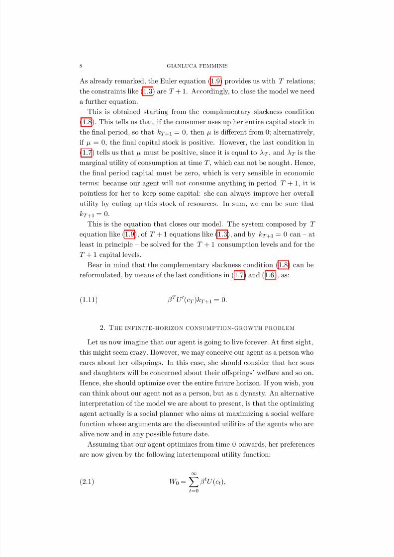
As already remarked, the Euler equation (1.9) provides us with T relations;
the constraints like (1.3) are T + 1. Accordingly, to close the model we need
a further equation.
This is obtained starting from the complementary slackness condition
(1.8). This tells us that, if the consumer uses up her entire capital stock in
the …nal period, so that kT +1 = 0; then is di¤erent from 0; alternatively,
if = 0; the …nal capital stock is positive. However, the last condition in
(1.7) tells us that must be positive, since it is equal to T ; and T is the
marginal utility of consumption at time T ; which can not be nought: Hence,
the …nal period capital must be zero, which is very sensible in economic
terms: because our agent will not consume anything in period T + 1; it is
pointless for her to keep some capital: she can always improve her overallutility by eating up this stock of resources. In sum, we can be sure that
kT +1 = 0:
This is the equation that closes our model. The system composed by T
equation like (1.9), of T + 1 equations like (1.3), and by kT +1 = 0 can – at
least in principle – be solved for the T + 1 consumption levels and for the
T + 1 capital levels.
Bear in mind that the complementary slackness condition (1.8) can be
reformulated, by means of the last conditions in (1.7) and (1.6), as:
(1.11) T U 0(cT )kT +1 = 0:
2. The infinite-horizon consumption-growth problem
Let us now imagine that our agent is going to live forever. At …rst sight,
this might seem crazy. However, we may conceive our agent as a person who
cares about her o¤springs. In this case, she should consider that her sons
and daughters will be concerned about their o¤springs’ welfare and so on.
Hence, she should optimize over the entire future horizon. If you wish, you
can think about our agent not as a person, but as a dynasty. An alternative
interpretation of the model we are about to present, is that the optimizing
agent actually is a social planner who aims at maximizing a social welfare
function whose arguments are the discounted utilities of the agents who are
alive now and in any possible future date.
Assuming that our agent optimizes from time 0 onwards, her preferences
are now given by the following intertemporal utility function:
(2.1) W 0 =
1
Xt=0
tU (ct);

8/15/2019 Feminis
http://slidepdf.com/reader/full/feminis 13/82
DYNAMIC PROGRAMMING: A PRIMER 9
The above expression is analogous to (1.1), but for the fact that now the
agent’s horizon extends up to in…nity.
Our problem is now to
max W 0 = max1X
t=0
tU (ct);
but, while the constraints are given by equations such as (1.3), the fact that
the consumer’s planning horizon is in…nite implies that we cannot impose a
“terminal constraint” like (1.4).
In this case, the consumer’s problem is tackled by means of the following
“present value” Lagrangian:
L0 = U (c0) + U (c1) + ::: + tU (ct) + :::(2.2)
0[k1 f (k0) (1 )k0 + c0]
:::
tt[kt+1 f (kt) (1 )kt + ct]
::::
Problem (2.2) di¤ers from (1.5) because it involves an in…nite number
of discounted utility terms, and an in…nite number of dynamic constraints;
moreover – as already remarked – the constraint concerning the …nal levelfor the stock variable is missing.
We optimize (2.2) with respect to ct, kt+1, and t for t = 0; 1;::::: ob-
taining:
(2.3) U 0(ct) = t; 8 t;
(2.4) tt = t+1t+1[f 0(kt+1) + (1 )]; 8 t;
and, of course:
(2.5) kt+1 = f (kt) + (1 )kt ct; 8 t:
These conditions are necessary, but they are not su¢cient: a “…nal condi-
tion” is missing. In our in…nite horizon model, the role of this …nal condition
is played by the so-called transversality condition (henceforth tvc), whichin
this set upis:
(2.6) limT !1
T
U
0
(cT )kT +1 = 0:

8/15/2019 Feminis
http://slidepdf.com/reader/full/feminis 14/82
10 GIANLUCA FEMMINIS
Comparing the above expression with (1.11), we immediately notice that
(2.6) is the limit, for T ! 1, of (1.11). This suggests us that the tvc
plays the role of the “missing” terminal condition. The tvc has a clear
economic interpretation: it rules out policies implying a “too fast” capital
accumulation in the long run. To understand this point, assume that our
consumer follows a policy implying a growing capital stock. Of course, this
capital would be accumulated at the expenses of consumption. Hence, this
policy would imply a high marginal utility of consumption, and an high and
increasing value for the product U 0(cT )kT +1: This, in itself, does not involve
the violation of condition (2.6). In fact, condition (2.6) allows U 0(cT )kT +1
to increase over time. Nevertheless, this growth must be slow enough to
be compensated by the convergence to 0 of the term T
: This is why wesay that the transversality condition rules out policies implying a “too fast”
long-run capital accumulation.
2.1. The qualitative dynamics. In our model, as it happens in many
in…nite horizon frameworks, it is useful to draw the phase diagram. To do
this, we …rst consider the stability loci for each of the two variables (i.e. we
compute where ct+1 = 0 and kt+1 = 0): This will help us to understand
how consumption and capital change over time whenever they are not on
their stability loci. Finally, we will jointly consider our knowledge for the
dynamics of the two variables.As for consumption, combining equation (2.4) with (2.3), we immediately
see that optimality requires that the Euler equation (1.9) is satis…ed. We
already know that the Euler equation is useful to describe the evolution
of consumption over time. In particular, we know that when kt = k; then
ct+1 = ct and hence ct+1 = 0 (consider again how we obtained Eq. (1.10)).
Hence, in Figure 1, we plot the locus implying stationarity for consumption
as a the vertical line drawn at k.
[Insert Figure 1]
Whenever kt < k; it is optimal for our consumer to increase her con-
sumption over time (hence, ct < ct+1). When kt > k; consumption must be
shrinking over time (ct+1 < ct): This behavior is summarized by the arrows
in Figure 1.
From Eq. (2.5), we see that kt+1 = f (kt) kt ct; hence, capital is
stationary when
(2.7) ct = f (kt) kt:

8/15/2019 Feminis
http://slidepdf.com/reader/full/feminis 15/82
DYNAMIC PROGRAMMING: A PRIMER 11
This relation can be portrayed as a function starting at the origin (by
assumption (c)), with a maximum at k
¯
(de…ned as the capital level such that
f 0(k ¯
) = ); and intersecting again the ct = 0 axis at k (which is the capital
level such that ct = 0; i.e. it is obtained solving the equation f (k) k = 0):11
The behavior of the kt+1 = 0 locus is portrayed in Figure 2.
[Insert Figure 2]
To see what happens when the economic system is not on the stability
locus (2.7), pick a capital level ~k 2 [0; k]; the corresponding consumption
level guaranteeing stationarity for capital obviously is
~c = f (~k) ~k:
If the consumer chooses a consumption level ct > ~c; her capital stock must
decrease over time: the consumption is so high that our consumer lives using
up part of her capital. More precisely, consumption is higher than the level,
~c; guaranteeing that the di¤erence between gross production, f (~k), and con-
sumption is exactly equal to capital depreciation ~k: Therefore the capital
stock must decrease: The converse happens when our consumer chooses a
consumption level ct that is lower than ~c: her capital increases over time
because a consumption lower than ~c implies that there is room for some sav-
ings, and hence there is some net investment. This behavior is summarizedby the arrows in Figure 2.
Merging Figures 1 and 2, we obtain Figure 3, which summarizes the dy-
namics of the model.
[Insert Figure 3]
Notice that there are three steady states (E; the origin, and I ). It is easy
to see that E is a steady state: here the two loci kt+1 = 0 and ct+1 = 0
intersect. Notice that the consumption and capital level characterizing this
steady state can be obtained solving the system
(2.8)
( 1 = [f 0(k) + (1 )]
c = f (k) k :
From Eqs. (1.9) and (2.7) it is clear that at E both consumption and
capital are not pressed to change over time.
The origin is a resting point because of Assumption (c): if capital is 0,
there is no production and hence no possibility of further capital accumula-
tion. This resting point is usually considered uninteresting.
11Existence and uniqueness of k are granted by assumptions (b) and (e).
8/15/2019 Feminis
http://slidepdf.com/reader/full/feminis 16/82
12 GIANLUCA FEMMINIS
It is less obvious that also I is a steady state. To gain some intuition
about the reason why I is a steady state, consider that the marginal utility
of consumption increases very rapidly as consumption approaches 0 (This
is because we assumed that limct!0 U 0(ct) = 1:) Hence, the increase in
the marginal utility of consumption prescribed by Eq. (1.9) for kt > k
implies smaller and smaller reductions in consumption as ct approaches 0.
Hence consumption does not become negative (which would of course have
no economic meaning) and I is a resting point.
A less heuristic argument is presented in the next three paragraphs, that
can be skipped by the uninterested reader.
To see that I is a steady state, rewrite (1.9) as:
U 0(ct+1) = U 0(ct)
1
[f 0(kt+1) + (1 )]
:
Pick a capital level, say ~k, belonging to the interval (k; 1): it is easy to
see that f 0(~k) + (1 ) 2 (1 ; 1= ): this comes from (1.10) and from
the assumptions: limkt!1 f 0(kt) = 0; and f 00(kt) < 0: Therefore, when~k 2 (k; 1); the term in the big square brackets in the equation above must
be larger than one: the largest value for the denominator is “slightly smaller”
than one: Therefore, the Euler equation not only tells us that the marginal
utility of consumption must increase (and hence that consumption mustdecrease), but also that the rate of change of marginal utility is limited,
being:
U 0(ct+1) U 0(ct)
U 0(ct) =
1
[f 0(~k) + (1 )] 1:
The value of the right hand side of the expression above belongs to the
interval
0; 1(1) 1
: This has a relevant implication: because the rate
of change of the marginal utility is bounded, when we consider a sequence
of consumption levels that – starting from a non negative value – ful…lls
the Euler equation, we see that this sequence cannot go to zero in …nitetime. This is because the marginal utility of consumption cannot “reach
in…nity” in …nite time (bear in mind that limct!0 U 0(ct) = 1). Because
consumption takes an “in…nite time” to reach its limiting value (that is,
0), in the meantime capital must reach k (since consumption decreases, the
system must reach at some time the area below the kt+1 = 0 locus where
capital grows, approaching k): Hence I is a stationary state for our system.
Let us now consider that our consumer is constrained by the fact that
her initial stock of capital is given (at k0). Hence, in choosing her optimal
consumption path, she must take into account this constraint. In Figure 3,
8/15/2019 Feminis
http://slidepdf.com/reader/full/feminis 17/82
DYNAMIC PROGRAMMING: A PRIMER 13
we have depicted some of the possible paths that our agent may decide to
follow. These paths are intended to ful…ll the Euler equation (1.9) and the
capital accumulation constraint (1.3).12
The fact that there are many (actually, in…nitely many) trajectories that
are compatible with one initial condition cannot be surprising: while the
capital stock k0 is given, our consumer is free to pick her initial consump-
tion level, which then determines the path for consumption and capital (via
equations (1.9) and (1.3)).
2.2. The optimal path. So far, we have seen that there are multiple paths
compatible with the same initial condition. What we need to do now, is to
select the optimal one(s).First, notice that the trajectory starting at A in Figure 3 cannot be op-
timal: because consumption is ever-increasing, capital must go to zero in
…nite time. Since by assumption capital is essential in production, at that
time consumption must collapse, becoming nought. This big jump in con-
sumption violates the Euler equation (which, to be ful…lled, would require
a further increase in consumption). In fact, the path starting at A – ad all
the paths akin to this one – cannot be optimal.
Second, consider the trajectory starting at B: In this case, our consumer
chooses exactly the consumption level that leads the system to the stationary
point E: This path not only ful…lls the di¤erence equations (1.9) and (1.3)
but also the transversality condition (2.6). In fact, as time goes to in…nity
(i.e. as t ! 1), capital and consumption approach their steady state levels,
k and c, which are given by System (2.8). The fact that the long run
levels for consumption and capital are positive and constant, tells us that,
in the steady state, the marginal utility of consumption is …nite. Hence,
limt!1 tU 0(ct)kt+1 = limt!1 tU 0(c)k = 0 simply because < 1; and this
second trajectory is optimal.
Third, consider the trajectory starting at C and leading to I : In this case,
consumption and capital …rst increase together, but then consumption (ascapital becomes larger than k) starts to shrink while capital is still accumu-
lated. In the long run, our optimizing agent …nds herself around I ; devoting
all the productive e¤ort to maintain an excessive stock of capital, which is
actually never used to produce consumption goods. Clearly following this
trajectory cannot be optimal, and the transversality condition is violated,
because the marginal utility of consumption tends to be in…nite.
12It is not possible to check that our paths in Figure 3 conform exactly to what is prescribedby our di¤erence equation. However, notice that they have been drawn respecting the
“arrows” that have been obtained from the di¤erence equations (1.9) and (1.3).
8/15/2019 Feminis
http://slidepdf.com/reader/full/feminis 18/82
14 GIANLUCA FEMMINIS
In the next two paragraphs, that can be skipped, we give a less heuristic
idea of the reasons why a path like the one starting at C violates the tvc.
To check whether a path of this type ful…lls the tvc, imagine to be “very
close” to I : Here, capital is (almost) k; hence consumption should (approx-
imately) evolve according to:
U 0(ct+1) = U 0(ct) 1
[f 0(k) + (1 )]:
Therefore:
U 0(ct+1) = U 0(ct) 1
[f 0(k) + (1 )] > U 0(ct);
where the latter inequality comes from the fact that for kt 2 (k ¯
; k); f 0(kt) +
(1 ) < 1 (at k ¯
; f 0(k ¯
) = ; and f 00(kt) < 0)). Because “around” k;
U 0(ct+1) > U 0(ct); limt!1 tU 0(ct) > 0 (Suppose that at a given time
T our system is already “very close” to I: In this case, in the following
periods, i.e. for t > T ; tT U 0(ct) > U 0(cT ): Hence limt!1 tU 0(ct) =
limt!1 T tT U 0(ct) > T U 0(cT )) Hence, the tvc (2.6) is not ful…lled and
any trajectory like the one starting at C is not optimal.
Summing up, the unique optimal path is the one leading to the steady
state E ; this path prescribes a monotonic increasing relation between con-sumption and capital. Our consumer (or our economic system) “jumps” on
this path by adjusting the initial consumption to the level compatible with
the existing capital stock, and with the behavior prescribed by our optimal
trajectory.
3. The Dynamic Programming formulation
In this Section, we solve the in…nite-horizon growth model exploiting the
dynamic programming approach: we shall take advantage of our previousunderstanding of the solution to introduce this new technique in an intuitive
way.
Consider again the intertemporal utility function (2.1). Obviously, our
optimizing agent’s preferences can be written as:
W 0 = U (c0) +1X
t=1
tU (ct):
In the formulation above, we have “separated” the utility obtained in the
current period, 0; from the ones that will be grasped in the future, but there
is no change in the meaning for W 0:

8/15/2019 Feminis
http://slidepdf.com/reader/full/feminis 19/82
DYNAMIC PROGRAMMING: A PRIMER 15
Notice that the expression above can be reformulated as:
(3.1) W 0 = U (c0) +
" 1Xt=1
t1U (ct)
#:
Here, we have collected the factor that is common to all the addenda
expressing future utilities. The reason for this manipulation is that the term
in the big square brackets represents the consumer’s preferences from the
perspective of time 1:
The problem we want to solve now is the very same we faced in the
previous Section: we wish to
max W 0 = max1X
t=0
tU (ct);
under the constraints given by equation (1.3), for t = 0; 1; ::::. Hence, we
wish to determine the optimal consumption ct , and kt+1; for t = 0; 1;:::.
Equation (3.1) allows us to write our problem as:
(3.2) max W 0 = max
(U (c0) +
" 1Xt=1
t1U (ct)
#):
Now consider, in Figure 4, the optimal path starting from B and ap-
proaching E . This trajectory represents a function, say '(:); relating opti-
mal consumption to the same period capital stock. We mean that c1 can
be expressed as c1 = '(k1); that c2 can be viewed as c2 = '(k2); and so
on. The function ct = '(kt) is unknown, and it can be very complex; actu-
ally what usually happens is that our function '(:) cannot be expressed in
a closedform analytical way. Nevertheless, the point that we underscore
here is that Figure 4 powerfully supports the idea that we have just stated,
i.e. that we can consider the optimal consumption as a function of contem-
poraneous capital. It is worth underscoring that our function ct = '(kt) is
“stationary”: it is always the same function, irrespective of the time periodwe are considering. Hence, the time dimension of the problem disappears.
The intuition to understand why '(:) is independent of time is to consider
our consumer’s perception of the future: because she lives forever, at time
0 her horizon is in…nite, and so it is at time 1. Hence, she must not ground
her decision on time, but just on capital, which therefore is the unique state
variable in our model.
[Insert Figure 4]

8/15/2019 Feminis
http://slidepdf.com/reader/full/feminis 20/82
16 GIANLUCA FEMMINIS
Notice that we have not proved that '(:) is continuous and di¤erentiable.
However, the evolution of capital and consumption on the optimal path
must ful…ll equations (1.9) and (1.3), which are continuos and di¤erentiable.
Hence, we have “good reasons to believe” that '(:) actually is continuous
and di¤erentiable, and we skip the formal proof for these statements.
Now consider that if we can write c1 = '(k1); then we are also able to
express the capital stock at time 2 as a function of k1: in fact, from (1.3),
k2 = f (k1) + (1 )k1 c1;
hence, on the optimal path:
k2 = f (k1) + (1 )k1 '(k1) = (k1):
The fact that k2 = (k1); allows us to consider the time 2 consumption
as a function of k1: c2 = '(k2) = '((k1)):
The important point here is to realize that we can iterate this reasoning
to express the whole sequence of optimal consumptions as a function of the
time 1 capital stock . (In fact, in general, kt+1 = (kt); and ct+1 = '(kt+1) =
'((kt)); and we can iterate the substitutions until we reach k1).
Hence, when consumption is optimally chosen from period 1 onward, the
group of addenda in the big square brackets in (3.2) can be expressed as a
function of k1 alone:1X
t=1
t1U (ct ) = V (k1):
V (k1) is a “maximum value function”: it represent the maximum lifetime
utility that can be obtained in period 1, when all the consumption levels are
optimally chosen given the available capital stock and the need to ful…l the
constraints of the (1.3)-type.
Because the value of all the future choices can be summarized in the func-
tion V (k1); we can think about the consumer’s intertemporal maximization
problem in a way that is di¤erent from the initial one. We can imagine that,at time 0, she picks her optimal period 0 consumption, taking account of the
fact that, given the available capital, an increase in current consumption re-
duces the future capital stock (via equation (1.3)), and therefore negatively
a¤ects the future overall utility V (k1):
Accordingly, the consumer’s intertemporal problem can be written as:

8/15/2019 Feminis
http://slidepdf.com/reader/full/feminis 21/82
DYNAMIC PROGRAMMING: A PRIMER 17
maxc0 fU (c0) + V (k1)g ;
s:t: k1 = f (k0) + (1 )k0 c0;
k0 given.
Now, imagine that our consumer solves her period 0 constrained optimiza-
tion problem, which means that she determines c0 as a function of k0. Our
representative consumer, obtaining c0; determines also her time 0 maximum
value function, V (k0), which means that
V (k0) = maxc0 fU (c0) + V (k1)g ;
s:t: k1 = f (k0) + (1 )k0 c0;(3.3)
k0 given.
The above problem is said to be expressed as a “recursive procedure” or
as a “Bellman equation”.
While it is easy to understand that problem (3.3) gets its name from
Bellman’s [1957] book, it is not so simple to explain in plain English what
a recursive procedure is.
Let us try. A procedure is recursive when one of the steps that makes
up the procedure requires a new running of the procedure. Hence, a recur-
sive procedure involves some degree of “circularity”. As a simple example,
consider the following “recursive” de…nition for the factorial of an integer
number:
«if n > 1; then the factorial for n is n! = n(n 1)!;
when n = 1, then 1! = 1».
Clearly, the above procedure de…nes n! by means of (n1)!; that is de…ned
exploiting (n 2)! and so on. This procedure goes on until 1 in reached, at
this point the “termination clause”, 1! = 1; enters into stage.
The logic of problem (3.3) is quite similar: the maximum value V (k0)
is obtained choosing the current consumption to maximize the sum of the
current utility and of the next-period discounted maximum value, which,
in turn is obtained by choosing future consumption in order to maximize
the sum of the future period utility and of the two periods ahead maximum
value ....
The di¤erence between (3.3) and the factorial number example lies in the
fact that our Bellman equation does not have a termination clause. This
is due to the fact that the planning horizon for our representative agent is
8/15/2019 Feminis
http://slidepdf.com/reader/full/feminis 22/82
18 GIANLUCA FEMMINIS
in…nite. If she were to optimize only between period 0 and a given period T
– for example, because she is bound to die at T – it would have been natural
to introduce a terminal condition: in this case, the maximum value at time
T + 1; for any stock of capital kT +1; would have been equal to nought (as
discussed in Sub-section 1.3).
Notice that the example we have just sketched implies that the maximum
value function depends not only on capital, but also on time. In fact, when
the agent’s time horizon is …nite, the maximum value function typically
depends on the remaining optimization horizon: how long you are going
to be still alive typically matters a lot for you, and it also a¤ects how you
evaluate your stock of wealth. Accordingly, at time t the maximum value
function is characterized by some terms involving T t.In contrast – as already underscored – in problem (3.3) we have written
the maximum value function as depending only on capital. This sometimes
strikes sensitive students: in fact, considering V (kt) as a function of capital
alone , we imply that V (kt) does not change over time despite the fact that –
moving backward from time 1 to time 0 – we discount the previous maximum
value function, and then we add to it the term U (c0). In other words, in
problem (3.3), we have the very same function V (kt) both on the left and
on the right hand side.
The intuition to understand why V (kt) is independent of time is to con-
sider again that our consumer’s perception of the future is the same at time
0 and at time 1, simply because she lives forever. Hence, she bases her
consumption decision only on capital, which therefore is the unique state
variable in our model. Because the function V (kt) summarizes the optimal
consumption decisions from period t onward, this function depends only on
capital.
The independence of time of the maximum value function in in…nite hori-
zon frameworks is one of the reasons why these frameworks are so popular:
their maximum value function – having a unique state variable – is less com-
plex to compute. Notice however that the absence of a termination clausemakes the problem of …nding a solution conceptually more di¢cult . In fact,
when we have a terminal time, we know the maximum value function for
that period: this is just the …nal period utility function. Hence, we can
always solve the problem for the terminal time, and then work “backward”
toward the present. This simple approach is precluded in in…nite horizon
models. Solving a …nite horizon problem is similar to decide how to send
to the surface of the Moon a scienti…c pod, while the solution of an in…-
nite horizon model is analogous to …nding an optimal lunar orbit for the
pod. In the …rst case, you can analyze all the possible location to pick the

8/15/2019 Feminis
http://slidepdf.com/reader/full/feminis 23/82
DYNAMIC PROGRAMMING: A PRIMER 19
most convenient one, say the Tranquility sea. Then you realize that to send
your pod to the Tranquility sea, you need a lunar module; then working
backwardyou determine that a spaceship is needed to get close to the moon
and …nally you understand that it takes a SaturnV missile to move the
spaceship out of the Earth atmosphere. Notice that, in this case, you have
a clear hint on how to start to work out your sequence of optimal decisions,
and your sequence is composed of a …nite number of steps. On the contrary,
if you need to have the scienti…c pod orbiting around the Moon, your time
horizon is (potentially) in…nite, and you need to devise an in…nite sequence
of decisions. Moreover, because you pod is continuously orbiting, you do not
have a clearly speci…ed terminal condition from which to move backward.
When considering whether to formulate a dynamic problem in a recur-
sive way, bear in mind that we have been able to write our intertemporal
maximization problem in the form (3.3) because the payo¤ function and the
intertemporal constraint are time-separable. 13
In the dynamic programming jargon, the single period payo¤ (utility)
function is often called the return function , the dynamic constraint is referred
to as the transition function , while a function relating in an optimal way
the control variable(s) to the state variable(s) is called the policy function .
In our example, the policy function is c
t = '(kt):
Before studying how an in…nite horizon problem can be solved, we need
to understand under which conditions the solution for problem (3.3) exists
and is unique.
Stokey, Lucas, and Prescott [1989] assure us that
Theorem 1. If: i) 2 (0; 1), ii) the return function is continuous, bounded
and strictly concave, and iii) the transition function is concave, then the
maximum value function V (kt) not only exists and is unique, but it is also
strictly concave, and the policy function is continuous.
Assumption i) is usually referred to as the “discounting” hypothesis, As-
sumption ii) requires that the utility function U (ct) is continuous, bounded
and strictly concave, while Assumption iii) constrains the production func-
tion kt+1 = f (kt) + (1 )kt ct, which must be concave for any given
ct:
The above result is neat, but it su¤ers from a relevant drawback: it does
not allow us to work with unbounded utility functions, and hence we cannot
13Moreover, if our agent’s utility depended upon current and future (expected) consump-tion levels, we would need to tackle a time inconsistency problem. For a simple introduc-
tion to this speci…c issue, see de la Fluente [2000, ch. 12].

8/15/2019 Feminis
http://slidepdf.com/reader/full/feminis 24/82
20 GIANLUCA FEMMINIS
assume, for example, that U (ct) = ln(ct). In general, it does not seem to be
easy to justify an assumption that precludes utility to grow without bounds.14
Stokey, Lucas, and Prescott discuss the case of unbounded returns in some
details (see their Theorem 4.14); here we follow Thompson [2004] in stating
a more restrictive theorem that will however su¢ce for many applications.
Theorem 2. (A theorem for unbounded returns). Consider the dynamic
problem (3.3). Assume that 2 (0; 1); and that the term P
1
t=0 tU (ct) exist
and is …nite for any feasible path fktg1t=0 ; given k0. Then there is a unique
solution to the dynamic optimization problem.
Theorem 2 essentially restricts the admissible one-period payo¤s to se-quences that cannot grow too rapidly relatively to the discount factor.15 To
see how this theorem can be applied, consider for instance Figure 3. Clearly,
when k0 < k; capital cannot become larger than k. Hence, given k0 2 [0; k],
U (ct) is …nite, and so isP
1
t=0 tU (ct), for any feasible path fktg1t=0 :16
Let us now tackle the problem of …nding the solution for the Bellman
equation. This is a functional equation, because we must determine the
form of the unknown function V (:).
Problem (3.3) tells us that, to obtain V (k0), it is necessary to maximize,
with respect to c0, the expression U (c0) + V (k1). Provided that V (k1) iscontinuous and di¤erentiable – a point that we are ready to accept – the
necessary condition for a maximum is obtained by di¤erentiating U (c0) +
V (k1) with respect to the current consumption, which yields:
(3.4) U 0(c0) + V 0(k1)@k1
@c0= 0;
where, of course, @ k1=@c0 = 1; from the capital accumulation equation.
The …rst order condition above relates the control variable (current con-
sumption) with the current and future values of the state variable ( k0 and
14Unfortunately, the boundedness of the return function is an essential component of theproof for the results stated in Theorem 1. In fact, to prove existence and uniqueness forV (kt), one needs to use an appropriate …xed point theorem, because the function V (kt) isthe …xed point of problem (3.3); the proofs of …xed point theorems require the boundednessof the functions involved.15The idea behind the proof, that we skip, it that if the term
P1
t=0 tU (ct) exist andis …nite, then the maximum value function is …nite, and we can apply an appropriate…xed-point theorem. Thompson (2004) is a very good introduction to the existence issuesof the maximum value function. He also provides several result useful to characterizethe maximum value function. The key reference in the literature is Stokey, Lucas, andPrescott [1989], which is however much more di¢cult.16The conditions stated in Theorem 1 or 2 imply the ful…lment of Blackwell’s su¢cient
conditions for a contraction.

8/15/2019 Feminis
http://slidepdf.com/reader/full/feminis 25/82
DYNAMIC PROGRAMMING: A PRIMER 21
k1). Let us exploit the …rst order condition (3.4), the Bellman equation, and
the constraint (1.3) to form the system:
(3.5)
8>>><>>>:
V (k0) = U (c0) + V (k1);
k1 = f (k0) + (1 )k0 c0;
U 0(c0) = V 0(k1);
k0 given:
The above system must determine the form of the maximum value func-
tion V (:); k1; and c0, for a given k0. Notice that the “max” operator in
the Bellman equation has disappeared, simply because we have already per-
formed this operation, via Eq. (3.4). Now consider what we often do when
we deal with a functional equation: when we need to solve a di¤erence or a
di¤erential equation, we (try to) guess the solution. Here, we can proceed
in the same way. The next Section provides examples in which this strategy
is successful.
4. Guess and verify
4.1. Logarithmic preferences and Cobb-Douglas production. In this
Sub-section, we analyze a simpli…ed version of the Brock and Mirman’s
(1972) optimal growth model. We shall propose a tentative solution, and
then we shall verify that the guess provides the correct solution.
In this framework the consumer’s time horizon is in…nite, and her prefer-
ences are logarithmic:
(4.1) W 0 =
1Xt=0
t ln(ct);
with 2 (0; 1). Using the jargon, we say that we are analyzing the case of
a logarithmic return function. The production function is a Cobb-Douglas
characterized by a depreciation parameter as high as unity (i.e. = 1; hence
capital entirely fades away in one period). Accordingly, we have that
(4.2) kt+1 = Akt ct;
where the “total factor productivity” parameter A is a positive constant and
2 (0; 1):
Our problem is to solve:
V (k0) = maxc0
fln(c0) + V (k1)g ;
s:t: k1 = Ak0 c0;
k0 given.

8/15/2019 Feminis
http://slidepdf.com/reader/full/feminis 26/82
22 GIANLUCA FEMMINIS
The …rst order condition, corresponding to equation (3.4), is: 1=c0 =
V 0(k1): This condition must be exploited in the problem above to substitute
out consumption. This yields:
(4.3)
8><>:
V (k0) = ln([V 0(k1)]1) + V (k1)
k1 = Ak0 1
V 0(k1)
k0 given.
This formulation makes it apparent once again that the Bellman equation
is a functional equation: it involves the function V (:) and its derivative V 0(:);
the constraint incorporates the initial condition for the state variable. In
fact, once V 0(:) is known, because k0 is given, the constraint determines k1;
and therefore the evolution for the capital stock. Notice that system (4.3)
corresponds to (3.5), but for the fact that here we have directly substituted
out c0 thanks to the explicit formulation c0 = [V 0(k1)]1:
Our attack against the functional equation is conducted by means of a
tentative solution, which in this case takes the form:
(4.4) V (kt) = e + f ln(kt);
where e and f are two constants to be determined, i.e. two undetermined
coe¢cients. Spend a few seconds in considering the guess (4.4). It is a linear
transformation of the utility function, where the control variable has beensubstituted by the state variable. When trying to …nd a tentative solution,
it is usually sensible to proceed in this way, i.e. to start with a guess that is
similar to the return function.
Taking the guess seriously, and exploiting it in (4.3), we obtain, for a
given k0:
(4.5)
( e + f ln(k0) = ln
k1f
+ [e + f ln(k1)]
k1 = Ak0 k1
f
:
One immediately notices that the second equation may be solved for k1:
(4.6) k1 = f
1 + f Ak
0 :
Substituting the above result in the …rst equation in (4.5) gives:
e + f ln(k0) = ln
1
1 + f Ak
0
+
e + f ln
f
1 + f Ak
0
:
Exploiting the usual properties of logarithmic functions, we obtain:

8/15/2019 Feminis
http://slidepdf.com/reader/full/feminis 27/82
DYNAMIC PROGRAMMING: A PRIMER 23
e + f ln(k0) = ln 1
1 + f
+ln(Ak0 ) + e + f ln f
1 + f
+ f ln(Ak0 );
or:
e + f ln(k0) = ln (1 + f ) +
+ ln A + ln k0 + e + f ln(f ) f ln (1 + f ) + f ln A + f ln k0:
The above equation must be satis…ed for any k0 and for any admissible
value of the parameters A;; and : Hence, it must be true that:
( f = + f
e = ln (1 + f ) + ln A + e + f ln(f ) f ln (1 + f ) + f ln A :
From the …rst equation in the system above we obtain:
f =
1 :
Notice that f > 0; because ; 2 (0; 1). This implies V 0(k) > 0; a
sensible result which tells us that a richer consumer enjoys a higher overall
utility. Substituting f in the second equation gives:
e = 11
1 ln ( ) + ln (1 ) + 1
1 ln A
:
The equation above provides us with some intuition concerning the reason
why we need the assumption < 1: were this requirement not ful…lled, the
maximum value function would “explode” to in…nity.
Because f and e are independent of capital, our guess (4.4) is veri…ed.
Substituting f into (4.6), we obtain: k1 = Ak0 ; which is the speci…c
form of the function kt+1 = (kt) introduced in Section 3.
From the …rst order condition, we know that c0 = 1= [V 0(k1)] ; hence,
using our guess, the computed value for f; and the fact that k1 = Ak
0
;
we obtain: c0 = (1 )Ak0 ; which is the form of the function ct = '(kt)
in this example.
The consumption function c0 = (1 )Ak0 is a neat but somewhat
economically uninteresting result: it prescribes that the representative agent
must consume, in each period, a constant share (1 ) of her current
income, Ak0 :
Notice that our consumption function relates the control variable to the
state variable: hence, it is the policy function.
From k1 = Ak0 ; we can easily obtain the steady state level for capital,
that is: k = (A)1
1 :

8/15/2019 Feminis
http://slidepdf.com/reader/full/feminis 28/82
24 GIANLUCA FEMMINIS
Having already obtained the maximum value function, it is certainly funny
to ask ourselves to prove that it exits and is unique. Nevertheless, this is
exactly what we are going to do in the next …ve paragraphs. The reason is
that we wish to develop a line of reasoning that may be helpful also when it is
not possible to …nd a closed-form solution for the maximum value function.
The uninterested reader may skip these paragraphs. In this case, however,
Exercise 4 will prove rather di¢cult.
Recall that U (ct) = ln(ct); and that kt+1 = Akt ct: Notice that the path
for capital characterized by the fastest possible growth for capital itself is
obtained by choosing zero consumption at each period of time. This path is
given by k1 = Ak0 ; k2 = Ak
1 ; ::: Hence, in general, we have that
ln(kt+1) = ln(A) + ln(kt) = ln(A) + ln(A) + 2 ln(kt1) =
= ::: = (1 t+1)
1 ln(A) + t+1 ln(k0):
Notice also that the largest one-period utility is obtained by consuming
the entire output that the representative agent can produce in that period,
i.e.
U (ct) = ln(Akt ) = ln(A) + ln(kt):
Therefore, if we follow the policy prescribing to save everything up to
period t and then to consume the entire output, we obtain:
U (ct) = ln(A) + ln(kt) = 1 t+1
1 ln(A) + t+1 ln(k0):
Imagine, counterfactually, that the above policy could be followed in every
period. In this case, the lifetime utility for the representative agent would
be:
1
Xt=0
t ln(ct) =
1
Xt=0
t
1 t+1
1 ln(A) + t+1 ln(k0)
=
= 1(1 ) (1 )
ln(A) + 1
ln(k0):
It is obvious that the above expression is …nite. Clearly, any feasible path
would yield a lower lifetime utility, therefore, any feasible sequence of payo¤s
must be bounded (in present value), and this implies that the maximum
value function must also be bounded. BecauseP
1
t=0 tU (ct) exist and is
…nite for any feasible path, Theorem 2 applies and the maximum value
function is unique.

8/15/2019 Feminis
http://slidepdf.com/reader/full/feminis 29/82
DYNAMIC PROGRAMMING: A PRIMER 25
Exercise 1. Assume that i) the single period utility function is: ln(ct) +
ln(1 lt); where lt 2 [0; 1] is the share of time devoted to labour, and
> 0; ii) the dynamic constraint is kt+1 = Akt l(1)
t ct; where A > 0 and
0 < < 1: Find the value function, and the related policy functions.
(Hint: because we have two control variables, the …rst order conditions
....)
Exercise 2. (Habit persistence) Assume that i) the single period utility
function is: ln(ct) + ln(ct1); where > 0; ii) the dynamic constraint
is kt+1 = Akt ct; where A > 0 and 0 < < 1: Find the value function,
and the related policy function.
(Hint: consider past consumption as a state of the system, hence the value
function has two arguments: kt and ct1....)
Exercise 3. Assume that i) the single period utility function is: c1 t =(1 );
where 2 [0; 1)[ (1; 1); ii) the dynamic constraint is kt+1 = Akt ct; where
A > 0: Find the value function, and the related policy function.
Exercise 4. Provide – for the return and the transition functions used in
the previous exercise – a condition on such that the boundedness conditions
in Theorem 2 is satis…ed.
4.2. Quadratic preferences with a linear constraint. We now con-
sider a consumer, whose time horizon is again in…nite, characterized by“quadratic” preferences:
(4.7) W 0 =1X
t=0
t
" + ct
2c2t
; with 2 (0; 1):
Because the parameters and are assumed to be positive, the marginal
utility for our consumer is positive for ct < =; while it is negative for
ct > =: Hence, the single-period utility is maximum when ct = =;
which is called the “bliss point” in consumption (the corresponding utility
is " + 2=(2)).17 The intertemporal constraint is linear in the state variablekt:
(4.8) kt+1 = (1 + r)kt ct:
We may interpret kt as the consumer’s …nancial assets and r as the in-
terest rate. Notice that, because the utility function is strictly concave and
bounded and the transition function is concave, we can be sure that the
value function is unique and strictly concave (Theorem 1).
17We do not take a position about ": it can be positive, negative or nought. For example,a negative " implies that our consumer needs a minimal amount of consumption to start
enjoying life (and hence having a positive utility).

8/15/2019 Feminis
http://slidepdf.com/reader/full/feminis 30/82
26 GIANLUCA FEMMINIS
Our problem is to solve:
V (k0) = maxc0n
" + c0
2 c20 + V (k1)o
;
s:t: k1 = (1 + r)k0 c0;
k0 given.
As before, we …nd the …rst order condition, which is: c0 = V 0(k1).
From the dynamic constraint we obtain c0 = (1 + r)k0 k1; which is used
to substitute consumption out of the Bellman equation and out of the …rst
order condition. This yields
(4.9)8><>:
V (k0
) = " + [(1 + r)k0
k1
]
2[(1 + r)k
0 k
1]2 + V (k
1)
[(1 + r)k0 k1] = V 0(k1);
k0 given.
Notice that system (4.9) corresponds to (3.5), but for the fact that we
have substituted out c0 exploiting the linear constraint (4.8).
The logic of the solution method is the same we have experienced in
the previous example: accordingly, we now introduce the tentative solution,
which takes the same functional form of the return function:
(4.10) V (kt) = g + hkt + m
2 k2
t ;
where g; h; and m are the undetermined coe¢cients. The (small) di¤erence
with the example in Sub-section 4.1 is that in this case we shall set up a
three equations system, because we need to determine three coe¢cients.
From the second equation in (4.9), we obtain:
k0 = 1
1 + r
h
+
m
k1
:
The equation above grants us that – in the present example – the function
kt+1 = (kt) is linear.
Substituting the guess (4.10) for V (k0); and V (k1) in the …rst equation in
(4.9), and exploiting the above expression, we obtain a quadratic equation
in k1: Because this equation must be satis…ed for any value of k1, it must
be true that:
(4.11)8>>><>>>:
g + h1+r
h
+ m
2(1+r)2
h
2= " +
( h) ( h)2
2 + g
h1+r
m
+ m
(1+r)2
m
h
= m
+ ( h)m
+ h
m2(1+r)2
m
2= (m)2
2 + m
2
:
8/15/2019 Feminis
http://slidepdf.com/reader/full/feminis 31/82
DYNAMIC PROGRAMMING: A PRIMER 27
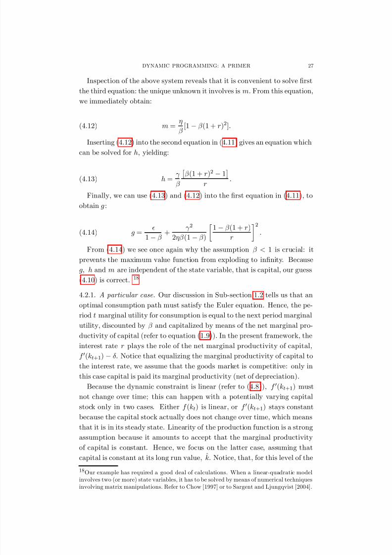
Inspection of the above system reveals that it is convenient to solve …rst
the third equation: the unique unknown it involves is m. From this equation,
we immediately obtain:
(4.12) m =
[1 (1 + r)2]:
Inserting (4.12) into the second equation in (4.11) gives an equation which
can be solved for h; yielding:
(4.13) h =
(1 + r)2 1
r :
Finally, we can use (4.13) and (4.12) into the …rst equation in (4.11), toobtain g :
(4.14) g =
1 +
2
2 (1 )
1 (1 + r)
r
2:
From (4.14) we see once again why the assumption < 1 is crucial: it
prevents the maximum value function from exploding to in…nity. Because
g; h and m are independent of the state variable, that is capital, our guess
(4.10) is correct. 18
4.2.1. A particular case. Our discussion in Sub-section 1.2 tells us that an
optimal consumption path must satisfy the Euler equation. Hence, the pe-
riod t marginal utility for consumption is equal to the next period marginal
utility, discounted by and capitalized by means of the net marginal pro-
ductivity of capital (refer to equation (1.9)). In the present framework, the
interest rate r plays the role of the net marginal productivity of capital,
f 0(kt+1) : Notice that equalizing the marginal productivity of capital to
the interest rate, we assume that the goods market is competitive: only in
this case capital is paid its marginal productivity (net of depreciation).
Because the dynamic constraint is linear (refer to (4.8)), f 0
(kt+1) mustnot change over time; this can happen with a potentially varying capital
stock only in two cases. Either f (kt) is linear, or f 0(kt+1) stays constant
because the capital stock actually does not change over time, which means
that it is in its steady state. Linearity of the production function is a strong
assumption because it amounts to accept that the marginal productivity
of capital is constant. Hence, we focus on the latter case, assuming that
capital is constant at its long run value, k: Notice, that, for this level of the
18Our example has required a good deal of calculations. When a linear-quadratic modelinvolves two (or more) state variables, it has to be solved by means of numerical techniques
involving matrix manipulations. Refer to Chow [1997] or to Sargent and Ljungqvist [2004].
8/15/2019 Feminis
http://slidepdf.com/reader/full/feminis 32/82
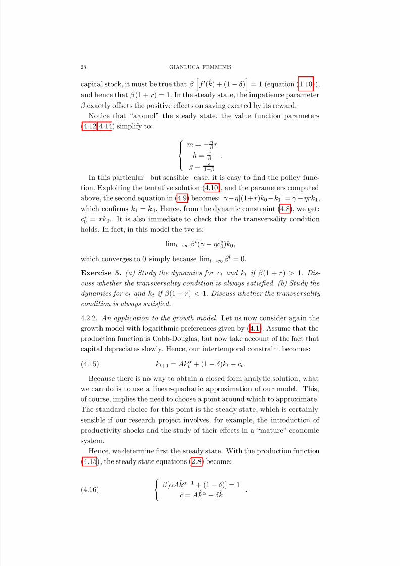
28 GIANLUCA FEMMINIS
capital stock, it must be true that
hf 0(k) + (1 )
i = 1 (equation (1.10)),
and hence that (1 + r) = 1: In the steady state, the impatience parameter
exactly o¤sets the positive e¤ects on saving exerted by its reward.
Notice that “around” the steady state, the value function parameters
(4.12-4.14) simplify to:
8><>:
m =
r
h =
g = 1
:
In this particularbut sensiblecase, it is easy to …nd the policy func-
tion. Exploiting the tentative solution (4.10), and the parameters computed
above, the second equation in (4.9) becomes: [(1+r)k0k1] = rk1;which con…rms k1 = k0: Hence, from the dynamic constraint (4.8), we get:
c0 = rk0. It is also immediate to check that the transversality condition
holds. In fact, in this model the tvc is:
limt!1 t( c0)k0;
which converges to 0 simply because limt!1 t = 0:
Exercise 5. (a) Study the dynamics for ct and kt if (1 + r) > 1: Dis-
cuss whether the transversality condition is always satis…ed. (b) Study the
dynamics for ct and kt if (1 + r) < 1: Discuss whether the transversality condition is always satis…ed.
4.2.2. An application to the growth model. Let us now consider again the
growth model with logarithmic preferences given by (4.1). Assume that the
production function is Cobb-Douglas; but now take account of the fact that
capital depreciates slowly. Hence, our intertemporal constraint becomes:
(4.15) kt+1 = Akt + (1 )kt ct:
Because there is no way to obtain a closed form analytic solution, what
we can do is to use a linear-quadratic approximation of our model. This,
of course, implies the need to choose a point around which to approximate.
The standard choice for this point is the steady state, which is certainly
sensible if our research project involves, for example, the introduction of
productivity shocks and the study of their e¤ects in a “mature” economic
system.
Hence, we determine …rst the steady state. With the production function
(4.15), the steady state equations (2.8) become:
(4.16) ( [Ak1 + (1 )] = 1
c = Ak
k
:

8/15/2019 Feminis
http://slidepdf.com/reader/full/feminis 33/82
DYNAMIC PROGRAMMING: A PRIMER 29
The above system allows to determine the consumption and capital steady-
state levels.19 We now apply Taylor’s theorem to the logarithmic utility
function, obtaining:
(4.17) ln(ct) = ln(c) + 1
c(ct c)
1
2c2(ct c)2:
As for the capital accumulation constraint, we truncate the Taylor’s ap-
proximation to the …rst term, which yields:
kt+1 = Ak + Ak1(kt k) + (1 )k + (1 )(kt k) c (ct c);
which immediately becomes:
kt+1 = Ak + (1 )k c +h
Ak1 + (1 )i
(kt k) (ct c);
and hence, using (4.16):
(4.18) kt+1 k = 1
(kt k) (ct c):
Equations (4.17) and (4.18) lead to the very same structure that can be
found in (4.7) and (4.8), and hence we can solve the approximate problem
using the tentative solution postulated for the linear-quadratic problem (therelevant variables are the deviations of capital and consumption from the
steady state).
5. Two useful results
The “guess and verify” technique is useful only when a closed form solu-
tion exists. Unfortunately, only a few functional forms for the payo¤ function
and for the dynamic constraint allow for a closed form maximum value func-
tion: the previous Section almost works out the list of problems allowing
for a closed form maximum value functions. Hence, we very often need to
“qualify” the solution, identifying some of its characteristics or properties,
without solving the model. In this Section, we review two important results,
that may be helpful in studying the solution for a Bellman equation.
5.1. The Envelope Theorem. We now apply the envelope theorem to
the standard growth model, as formulated in Problem (3.3). In other words,
we concentrate – for simplicity – on a speci…c application of the envelope
theorem. However, the results that we obtain, besides being important, are
of general relevance.
19Which are: k = A
1(1)
1
1
; and c = 1[1(1)]
A
1(1)
1
1
:

8/15/2019 Feminis
http://slidepdf.com/reader/full/feminis 34/82
30 GIANLUCA FEMMINIS
To save on notation, we now denote the dynamic constraint by k1 =
g(k0; c0), accordingly, the dynamic programming formulation for our utility-
maximization problem becomes:
V (k0) = maxc0
fU (c0) + V (k1)g ;
s:t: k1 = g(k0; c0); k0 given.
We already know that the …rst order condition with respect to the control
variable is U 0(c0) + V 0(k1) @k1@c0
= 0: Consider now the Bellman problem
above, assuming to be on the optimal path. In this case, we have V (k0) =
U (c0) + V (k1) (the max operator disappears exactly because we already
are on the path in which consumption is optimal). The total di¤erentialfor the last equation is: dV (k0) = dU (c0) + dV (k1); or: V 0(k0)dk0 =
U 0(c0)dc0 + V 0(k1)dk1: The di¤erential for k1 can be easily obtained from
the dynamic constraint: dk1 = gk(k0; c0)dk0 + gc(k0; c0)dc0: 20
Exploiting dk1, the total di¤erential for the Bellman equation becomes:
V 0(k0)dk0 = U 0(c0)dc0 + V 0(k1) [gk(k0; c0)dk0 + gc(k0; c0)dc0] :
This expression, using the …rst order condition for c0; reduces to:
V 0(k0) = V 0(k1)gk(k0; c0):
This is an application of the Envelope theorem: we have simpli…ed the
total di¤erential precisely because we are on the optimal path, and hence
the …rst order condition must apply.
Notice that we could have expressed the above result as follows:
(5.1) V 0(k0) = V 0(k1)@k1
@k0;
where @ k1=@k0 is the partial derivative, gk(k0; c0).
Equation (5.1) can be useful in several contexts. In fact, it can be refor-
mulated in a very convenient way. Because the …rst order condition statesthat: U 0(c0) = V 0(k1); it must also be true that U 0(c1) = V 0(k2): With
these facts in mind, we forward once equation (5.1), and we obtain:
(5.2) U 0(c0) = U 0(c1)gk(k1; c1);
which is the Euler equation (bear in mind that, in the growth example,
gk(k1; c1) = f 0(k1) + (1 ); and refer to (1.9)). Not only it is often easier
20We denote by a subscript the partial derivatives. Accordingly, gk(k0; c0) is the partialderivative of g(k0; c0) with respect to capital, and so on. This convention shall be adopted
whenever we need to di¤erentiate a function with two or more arguments.

8/15/2019 Feminis
http://slidepdf.com/reader/full/feminis 35/82
DYNAMIC PROGRAMMING: A PRIMER 31
to solve numerically equation (5.2) than Bellman’s one – as we shall see in
Sub-section 6.2 – but equation (5.2) can be interpreted without referring to
the still unknown maximum value function.
Notice that Equation (5.2) corresponds exactly to Equation (1.9): this
reassures us about the fact that the Bellman’s approach and the Lagrange’s
one lead to the same result.
5.2. The Benveniste and Scheinkman formula. In this Sub-section –
that can be skipped during the …rst reading – we consider a more general
framework, where the return function does not depend only on the con-
trol variables, but it also depends on the state. In this case the dynamic
programming formulation is:
V (k0) = maxc0
fQ(k0; c0) + V (k1)g ;
s:t: k1 = g(k0; c0); k0 given.
The …rst order condition with respect to the control variable yields:
Qc(k0; c0) + V k(k1)dk1dc0
= 0:
Assume, as in the previous Sub-section, to be on the optimal path, so that:
V (k0) = Q(k0; c0) + V (k1): The total di¤erential for the last equation is:dV (k0) = dQ(k0; c0) + dV (k1); or:
V k(k0)dk0 = Qc(k0; c0)dc0 + Qk(k0; c0)dk0 + V k(k1)dk1:
The di¤erential for the …rst period capital is obtained from the dynamic
constraint, and is dk1 = gk(k0; c0)dk0 + gc(k0; c0)dc0: Hence, the total di¤er-
ential for the Bellman’s equation becomes:
V k(k0)dk0 =
= Qc(k0; c0)dc0 + Qk(k0; c0)dk0 + V k(k1) [gk(k0; c0)dk0 + gc(k0; c0)dc0] :
Using the …rst order condition, the equation above reduces to:
(5.3) V k(k0) = Qk(k0; c0) + V k(k1)gk(k0; c0):
This is the Benveniste and Scheinkman formula, which can be obtained
as an application of the Envelope theorem.
The usefulness of the Benveniste and Scheinkman formula (5.3) can be
appreciated considering that, in many problems, there is not a unique way
to de…ne states and controls. For example, in the growth model, one could

8/15/2019 Feminis
http://slidepdf.com/reader/full/feminis 36/82
32 GIANLUCA FEMMINIS
de…ne as control variable not consumption, but gross savings (which means
that the control is st = f (kt) ct). When depreciation is complete, this
modi…cation implies that the next-period state is equal to the current control
(kt+1 = st), and the Bellman problem (3.3) with = 1, becomes:
V (k0) = maxs0
fQ[f (k0) s0] + V (k1)g ;
s:t: k1 = s0;(5.4)
k0 given.
With this formulation, the …rst order condition is: U 0[f (k0) s0] =
V 0(k1):
If we di¤erentiate the Bellman equation “on the optimal path”, we obtain:
V 0(k0)dk0 = Q0[f (k0) s0] [df (k0) ds0] + V 0(k1)dk1:
Because dk1=ds0 = 1; using the …rst order condition the di¤erential can
be reduced to:
(5.5) V 0(k0) = Q0[f (k0) s0]f 0(k0);
which is the Benveniste and Scheinkman formula in our context.
Formula (5.5) is interesting because it shows that the Benveniste andScheinkman result can be used to highlight a relation between the initial
period maximum value function, the return function and the dynamic con-
straint. The Benveniste and Scheinkmann formula leads to such relation
when the partial derivative of the dynamic constraint with respect to the
current state is 0 . For this to be true, it is necessary that the initial period
state variable (k0) is excluded from the dynamic constraint, as it happens
in problem (5.4). The example we have just developed shows that this can
be achieved by means of a proper variable rede…nition (see Sargent [1987]
pp. 21-26 for a discussion and an alternative example).
Exercise 6. Apply the Benveniste-Scheinkman formula to the standard
growth model, and show that the maximum value function is concave.
Exercise 7. By means of an appropriate variable rede…nition, show that the
Benveniste-Scheinkman formula (5.5) applies to the standard growth model
when < 1:
6. A “paper and pencil” introduction to numerical techniques
As already underscored, the “guess and verify” technique is useful only in
the few cases in which a closed form solution for the maximum value function
8/15/2019 Feminis
http://slidepdf.com/reader/full/feminis 37/82
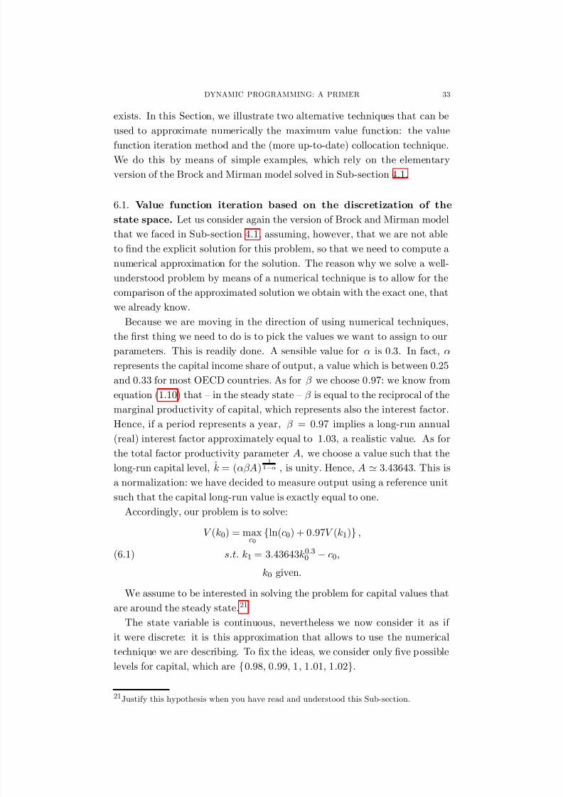
DYNAMIC PROGRAMMING: A PRIMER 33
exists. In this Section, we illustrate two alternative techniques that can be
used to approximate numerically the maximum value function: the value
function iteration method and the (more up-to-date) collocation technique.
We do this by means of simple examples, which rely on the elementary
version of the Brock and Mirman model solved in Sub-section 4.1.
6.1. Value function iteration based on the discretization of the
state space. Let us consider again the version of Brock and Mirman model
that we faced in Sub-section 4.1, assuming, however, that we are not able
to …nd the explicit solution for this problem, so that we need to compute a
numerical approximation for the solution. The reason why we solve a well-
understood problem by means of a numerical technique is to allow for thecomparison of the approximated solution we obtain with the exact one, that
we already know.
Because we are moving in the direction of using numerical techniques,
the …rst thing we need to do is to pick the values we want to assign to our
parameters. This is readily done. A sensible value for is 0.3. In fact,
represents the capital income share of output, a value which is between 0.25
and 0.33 for most OECD countries. As for we choose 0:97: we know from
equation (1.10) that – in the steady state – is equal to the reciprocal of the
marginal productivity of capital, which represents also the interest factor.
Hence, if a period represents a year, = 0:97 implies a long-run annual
(real) interest factor approximately equal to 1:03, a realistic value. As for
the total factor productivity parameter A; we choose a value such that the
long-run capital level, k = (A)1
1 ; is unity. Hence, A ' 3:43643. This is
a normalization: we have decided to measure output using a reference unit
such that the capital long-run value is exactly equal to one.
Accordingly, our problem is to solve:
V (k0) = maxc0
fln(c0) + 0:97V (k1)g ;
s:t: k1 = 3:43643k
0:3
0 c0;(6.1)k0 given.
We assume to be interested in solving the problem for capital values that
are around the steady state.21
The state variable is continuous, nevertheless we now consider it as if
it were discrete: it is this approximation that allows to use the numerical
technique we are describing. To …x the ideas, we consider only …ve possible
levels for capital, which are f0:98; 0:99; 1; 1:01; 1:02g:
21Justify this hypothesis when you have read and understood this Sub-section.

8/15/2019 Feminis
http://slidepdf.com/reader/full/feminis 38/82
34 GIANLUCA FEMMINIS
Notice that, if we knew the function V (k1), it would be relatively easy
to solve problem (6.1): the solution would be the consumption level c0 that
allows to obtain the highest V (k0), provided that k0; k1 2 f0:98; 0:99; 1; 1:01;
1:02g: For example, assume that V (k1) = 20k1 (this choice is completely
arbitrary; actually we know that it is wrong: we just want to illustrate what
we mean when we say that – knowing V (k1) – it is easy to solve problem
(6.1)): When k0 = 0:98, the problem becomes:
V (k0 = 0:98) = maxc0
fln(c0) + 0:97 20k1g ;
s:t: k1 = 3:43643(0:98)0:3 c0;(6.2)
k0 = 0:98:
To tackle the problem, we must leave our standard tool – the deriva-
tive – on the shelf, because our problem is not continuous: we have de-
cided to compute V (k1) only in a few points. Hence, we need to per-
form all the required calculations. First, we express the constraint as:
c0 = 3:43643(0:98)0:3 k1 = 3:41566 k1; and we compute the consumption
levels that allow k1 to take one of the …ve feasible values. These are:
k1 0.98 0.99 1 1.01 1.02
c0 2.43566 2.42566 2.41566 2.40566 2.39566
Second, we consider the postulated maximum value function: for V (k1) =
20k1 the right hand side of problem (6.2) takes, in correspondence of the
…ve couples fk1; c0g computed above, the following values:
r:h:s:(6:2) 19.90222 20.09210 20.28197 20.47182 20.66166
According to the above calculations, the highest value is obtained for
the consumption choice c0 = 2:39566, hence V (k0 = 0:98) takes the value
20.66166.
This calculation should be repeated for every remaining k0
2 f0:99; 1;
1:01; 1:02g, this would give us the period 0 maximum value function for
each state.
However, there is no need to perform all these calculations: the point we
wish to underscore here is that the few calculations we have presented above
are already enough to conclude that the postulated function V (k1) = 20k1; is
incorrect. From our analysis in Section 3, we know that – in in…nite horizon
models – the maximum value function is time independent. Accordingly,
the functional form we have assumed for period 1 must apply also to period
0. Hence, we should expect to …nd that V (k0 = 0:98) = 19:6, which is not
the case.
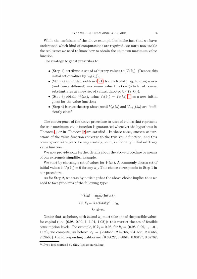
8/15/2019 Feminis
http://slidepdf.com/reader/full/feminis 39/82
DYNAMIC PROGRAMMING: A PRIMER 35
While the usefulness of the above example lies in the fact that we have
understood which kind of computations are required, we must now tackle
the real issue: we need to know how to obtain the unknown maximum value
function.
The strategy to get it prescribes to:
(Step 1) attribute a set of arbitrary values to V (k1): (Denote this
initial set of values by V 0(k1));
(Step 2) solve the problem (6.1) for each state k0, …nding a new
(and hence di¤erent) maximum value function (which, of course,
substantiates in a new set of values, denoted by V 1(k0));
(Step 3) obtain V 2(k0); using V 1(k1) = V 1(k0) 22
as a new initialguess for the value function;
(Step 4) iterate the step above until V n(k0) and V n+1(k0) are “su¢-
ciently close”.
The convergence of the above procedure to a set of values that represent
the true maximum value function is guaranteed whenever the hypothesis in
Theorem 1 or in Theorem 2 are satis…ed. In these cases, successive iter-
ations of the value function converge to the true value function, and this
convergence takes place for any starting point, i.e. for any initial arbitrary
value function.We now provide some further details about the above procedure by means
of our extremely simpli…ed example.
We start by choosing a set of values for V (k1): A commonly chosen set of
initial values is V 0(k1) = 0 for any k1. This choice corresponds to Step 1 in
our procedure.
As for Step 2, we start by noticing that the above choice implies that we
need to face problems of the following type:
V (k0) = maxc0 fln(c0)g ;
s:t: k1 = 3:43643k0:30 c0;
k0 given.
Notice that, as before, both k0 and k1 must take one of the possible values
for capital (i.e. f0:98; 0:99; 1; 1:01; 1:02g): this restrict the set of feasible
consumption levels. For example, if k0 = 0:98, for k1 = f0:98; 0:99; 1; 1:01;
1:02g; we compute, as before: c0 = f2:43566; 2:42566; 2:41566; 2:40566;
2:39566g; the corresponding utilities are f0:89022; 0:88610; 0:88197; 0:87782;
22If you feel confused by this, just go on reading.
8/15/2019 Feminis
http://slidepdf.com/reader/full/feminis 40/82
36 GIANLUCA FEMMINIS
0:87366g: The highest utility level is reached for c0 = 2:43566; which is the
consumption level implying that the next period capital is k1 = 0:98:
Hence, the solution for this speci…c problem is V 1(k0 = 0:98) = 0:89022:
Repeating this reasoning we obtain: V 1(k0 = 0:99) = 0:89449; V 1(k0 =
1) = 0:89871; V 1(k0 = 1:01) = 0:90288; V 1(k0 = 1:02) = 0:90701: In every
problem, the solution corresponds to the maximum feasible consumption
level, which is the one corresponding to k1 = 0:98. In other words, for
any k0 2 f0:98; 0:99; 1; 1:01; 1:02g; c0 is such that k1 = 0:98. This is
hardly surprising: since we have arbitrarily chosen V 0(k1) = 0; capital bears
no future value, and hence it is sensible to choose to consume as much as
possible.23
The key point is that our maximization procedure has led to a set of values for V 1(k0): Accordingly, we have completed Step 2 in the procedure.
Hence – Step 3 – we use these values as a new guess for the maximum
value function. This bit of the procedure is inspired by the fact that the
true maximum value function is time independent: at di¤erent dates it must
take the same values for any capital stock. Accordingly, we now assume
V 1(k1) = f0:89022; 0:89449; 0:89871; 0:90288; 0:90701g:
In this second iteration for the maximization problem, when k0 = 0:98,
consumption may again take the values c0 = f2:43566; 2:42566; 2:41566;
2:40566; 2:39566g: When c0 is 2:43566; (that is, when it takes the value
guaranteeing k1 = 0:98), the corresponding “overall utility” is ln(2:43566)
plus times V 1(k1 = 0:98) = 0:89022 (which gives V 2(k0 = 0:98) = 1:75373):
In words, this is the “overall value” obtained by choosing the consumption
level that allows to transfer the current capital level to the next period.
Considering the whole set of choices, c0 = f2:43566; 2:42566; 2:41566;
2:40566; 2:39566g; we …nd that the values associated are {ln(2:43566) +
0:97 0:89022; ln(2:42566) + 0:97 0:89449; ln(2:41566) + 0:97 0:89871;
ln(2:40566)+0:970:90288; ln(2:39566)+0:970:90701g; which are f1:75373;
1:75376; 1:75372; 1:75362; 1:75346g:
Notice that the second value in the row, 1:75376 is the highest one. Hence,the optimal choice is now to opt for a consumption level such that the next
period capital is 0:99: In words, if the initial capital is 0.98 and if we take
account of the future period (discounted) utility, it is optimal to save 0.01
units of capital.
When we repeat this reasoning for the other capital values in our grid,
we obtain that: if k0 = 0:99, the consumption optimal choice is such that k1
remains at 0:99; when k0 = 1, the consumption optimal choice is such that k1
is again 0:99; when k0 = 1:01 or 1:02, the consumption optimal choice is such
23Here the logic is the same we used in Sub-section 1.3 to argue that kT +1 = 0:

8/15/2019 Feminis
http://slidepdf.com/reader/full/feminis 41/82
DYNAMIC PROGRAMMING: A PRIMER 37
that k1 = 1: In correspondence to the optimal choices described above, the
value function is: V 2(k1) = f1:75376; 1:75804; 1:76228; 1:76649; 1:77065g:
The obtaining of this set of values concludes Step 3 in our procedure.
Of course, a normal person is already fed up with all these calculations.
This is the point to let our computer do the calculations, hence performing
Step 4. It is easy to write a program using Matlab (or Gauss) that carries
out this task.24 The results of this program are reported in Table 1.
[Insert Table 1]
In the simulation, the convergence criterion we have chosen is as follows:
we let the computer calculatefor each gridpointthe di¤erence between
the …nal and the initial value of V (k0) (i.e. V n+1(k0) V n(k0)); then we
considered the absolute values of these di¤erences and we let the routine to
pick the largest. When this is below 10(5), we let the computer to stop. On
a 3 Ghz Pentium computer, this happens after about 30/100 of a second, at
the 376th iteration.
Because the computed value function converges to the true maximum
value function, when the set of values representing V n+1(k0) is “almost iden-
tical” to the one used to represent V n(k0); they are also “almost identical”
to the true set of values, which is to the true V (k0).
Having chosen an exercise for which we know the exact solution, we havebeen able to provide, as a reference point, the true values for V (k1):
Exercise 8. Check that the values for V (k) in the last line of Table 1 are
correct.
From Table 1, we can see that the values for V (k1) smoothly converge
toward their true value: we are in the position to “observe in action” the
(vector) …xed point nature of our problem.
In our case, the convergence is slow. This is due to the fact that is
close to unity: what happens in the future matters a lot, hence the initial
arbitrary values for V (k1) do not lose rapidly their weight.
The nice feature of this approach consist in the fact that it is immediate
to change the interval for the state variable and the number of gridpoints,
therefore adapting a numerical routine to a new situation. For example, we
can use the program written for the problem above to study what happens
for k 2 [0:7; 1:1] with 1600 gridpoints. Figure 5a plots the maximum value
function, while Figure 5b shows the di¤erences between the true value func-
tion and the approximated one. Notice that the computing time increases
dramatically: it takes about seventy-…ve minutes to achieve convergence.
24In the Appendix, we provide some details about the routines used to solve our examples.

8/15/2019 Feminis
http://slidepdf.com/reader/full/feminis 42/82
38 GIANLUCA FEMMINIS
[Insert Figure 5]
This is probably the right time to became aware of one of the sad facts of
life, which is usually referred to as “the curse of dimensionality”. By these
words, one usually refers to the fact that the speed of a procedure such as
the one we have brie‡y described decreases more than proportionally with
the number of state variables. To understand this fact, bear in mind that, to
…nd the value function by iteration, we have discretized the state space. In
our case, the state space is a line, because we have just one state variable,
that is physical capital. If we had two state variables, say physical and
human capital, we would have a 2-dimensional state space (which means,
a plane). In this case, it would have been necessary to divide the state
space is small “squares”, the number of which is of course the square of
the number of points we use to discretize each dimension. Accordingly, the
number of “evaluation points” increases with the power of the number of
state variables. Hence, the required computer time grows with the power
of the number of state variables. 25 For example, in a model where the
representative agent decides her consumption level and her schooling e¤ort
as functions of both human and physical capital, we need to compute the
value function for every combination of human and physical capital in the
two-dimensional grid.In short: if our problem is large, we need to use a more e¢cient technique,
which is the topic of the next Sub-section. Nevertheless, the value function
iteration method can be of some help when one or more dimensions of the
state space are naturally discrete. This happens when the researcher wishes
to study problems where the agent may be employed or unemployed, may
decide whether to get a degree or not, whether to retire or not, and so on.
This method can be of some help also if the transition function is subject to a
constraint. Suppose, to mention the most famous example, that investment
is irreversible, so that k1 k0(1 ): This problem can be easily dealt with
in our framework: it is su¢cient not to consider the consumption level thatimply an infringement of the irreversibility constraint. 26
25If one chooses a di¤erent number of grid points for the two state variables–thereforedividing the plane in small rectangles–the argument in the main text must be properlyadapted.26The presence of an irreversibility constraint is much more interesting in a stochasticmodel than in a deterministic one. Figure 3 suggests that whenever the initial capitalstock is below the steady-state, capital grows over time until it reaches its steady statevalue. Accordingly, an irreversibility constraint can bind only if our representative agentsreceives, as a gift, a capital level that is so much higher than the steady state one, thatshe wants to decumulate it at a fast rate. Instead, in a stochastic model, a shock may be
su¢cient to make the irreversibility constraint binding.
8/15/2019 Feminis
http://slidepdf.com/reader/full/feminis 43/82
DYNAMIC PROGRAMMING: A PRIMER 39
6.2. Collocation techniques. As already remarked, the previous tech-
nique is rather ine¢cient, because it requires the evaluation of the value
function in a large number of points. Here, we present a more e¢cient
method to solve dynamic models, which is known as “collocation technique”.
Because the application of this technique to a Bellman equation is rela-
tively complex, we move in small steps. We …rst underscore that the collo-
cation technique is a way to “approximate” or to “interpolate” a function.
Hence, it can be applied to any function, say to trigonometric or to expo-
nential ones, and not necessarily to a maximum value function. Second, we
show how this technique can be used to solve a simple – actually the simplest
– di¤erential equation, and …nally we deal with a Bellman problem.
To understand the idea underlying this technique, we need to introduce
the Weierstrass Theorem, which says:
Theorem 3. Any continuous real function f (x) can be approximated in a
interval X by a polynomial pn(x) =Pn
i=0 aixi:
The words “can be approximated” mean that for any number > 0; there
is a polynomial, of suitable degree, such that maxx2X jf (x) pn(x)j < : In
practice, a reduction in ; i.e. in the approximation error, usually calls for
an increase in the degree of the polynomial.27
This is interesting and rather intuitive, but it does not tell us how to
proceed in practice. Hence, let us consider a speci…c example, choosing a
relatively challenging function: imagine that we need to approximate sin(x)
over the interval X = [0; 2]. Let us start with the third degree polynomial,
p3(x) = a0 + a1x + a2x2 + a3x3: Our problem is to determine the four ai
coe¢cients so that our polynomial behaves as the sin(x) function in the
interval X . Because we need to determine four unknown coe¢cients, we
choose four points in X: In fact, evaluating sin(x) and p3(x) at these points,we obtain four equations in the ai’s, which can be solved for the unknown
coe¢cients.
Notice that, when the irreversibility constraint is binding, our consumer is forced to con-sume less than what would be optimal. Hence, she would like to avoid …nding herself inthis situation.Therefore, the awareness that then irreversibility constraint may be binding, even if witha low probability, is su¢cient to in‡uence the representative agent behavior. We shallbrie‡y return on models with stochastically binding constraints in Section (10.2).27Bear in mind, however, that the relation between and the degree of the approximating
polynomial is not always monotonic.

8/15/2019 Feminis
http://slidepdf.com/reader/full/feminis 44/82
40 GIANLUCA FEMMINIS
For example, choose x = f0; 2=3; 4=3; 2g:28 At these points, the col-
location method forces the approximating polynomial to be identical to the
function which needs to be approximated. This yields:
(6.3)
8>>><>>>:
0 = a0
0:86602 = a0 + a12:09440 + a24:38649 + a39:18704
0:86602 = a0 + a14:18879 + a217:54596 + a373:49636
0 = a0 + a16:28318 + a239:47842 + a3248:05021
Solving for the ais this linear system, one obtains that the approximating
third-degree polynomial is: 0 + 1:860680x 0:888409x2 + 0:094263x3.
For a “…rst impression judgement” of our results, we plot our polyno-
mial and the sin(x) function over [0; 2]: In Figure 6, the continuous line
represents sin(x); while the dashed line is its third degree approximation.
Some further calculations show that the largest di¤erence between the two
functions is 0.2554. This is a large number, nevertheless we can be fairly sat-
is…ed with our exercise: we have been able to approximate a trigonometric
function by means of a simple third degree polynomial.
[Insert Figure 6]
However, we must be aware that our approximation deteriorates rapidly
as we exit from the interval X = [0; 2] (compute p3(x) at 2:5!). The
rapid deterioration of the approximation outside the interval is a general
characteristic of the results obtained by means of this approach. The ap-
proximation of a function by means of the collocation method is similar to
what one can do with some pins and a ‡exible plastic stick: one takes the
stick (the polynomial) and the pins (the value of the polynomial at the col-
location points), and use the pins to …x the stick over the function. With a
decent number of pins, one can easily make a good job in the interval inside
the …rst and the last pin; outside this interval, the plastic stick keeps its
original shape.It is now time to leave aside once again paper and pencil. Choosing, for
example, eleven collocation points, and hence using a tenth degree polyno-
mial, we can easily build an eleven equations system. We can then use the
equation matrix manipulation facilities that are built-in in computation pro-
grams such as Matlab or Gauss to solve the system; with Matlab this should
take about 60/100 of a second.29 (You can deal with this problem also by
means of Mathematica or Maple). Figure 7 shows the approximation error
28Using the jargon, we say that we have chosen four evenly spaced “collocation points”or “nodes”.
29A system like (6.3) can be written in matrix form as:

8/15/2019 Feminis
http://slidepdf.com/reader/full/feminis 45/82
DYNAMIC PROGRAMMING: A PRIMER 41
for this exercise. The bright side is that we are really making a decent job,
the somehow dark side is that the errors are de…nitely higher than average
at the beginning and at the end of the interval. This is usually regarded as
a clear sign that we can improve our approximation.
[Insert Figure 7]
It is now possible to climb a step of the ladder that is bringing us to the
solution for the dynamic optimization problem. Up to now, we have shown
that we can approximate a function by means of a polynomial. Now consider
that the solution for a di¤erence or a di¤erential equation is a function (in
our example the solution is a function of time, which is the state variable
in this exercise). This suggests that we can approximate the solution for a
functional equation by means of our collocation technique.
As before, we choose a simple example, actually, we choose a di¤erential
equation that we are able to solve analytically. This will allow us to judge
the “goodness of …t” characterizing our exercise.
Suppose that we need to solve the …rst order linear di¤erential equation
(6.4) dx(t)
dt
= 0:1x(t) + 1; given x(0) = 2;
in the interval t 2 [0; 4]: Assume that the solution x(t) must be approxi-
mated by a second-degree polynomial: denoting with an upperbar the ap-
proximated solution, we have
(6.5) x(t) = a0 + a1t + a2t2:
A good approximation, behaving “almost like” the true solution x(t);
must ful…ll equation (6.4). Actually, the true solution must satisfy (6.4) for
any t; hence, it is more than reasonable to require that the approximation
ful…lls (6.4) “at least somewhere”, which means, in the collocation points.
There, the approximation must be such that:
dx(t)
dt = 0:1x(t) + 1;
which means, exploiting (6.5) in both sides of the last equation, that at the
collocation points it must be true that:
2664
1 0 0 01 2:09440 4:38649 9:187041 4:18879 17:54596 73:496361 6:28318 39:47842 248:05021
3775
2664
a0a1a2a3
3775 =
2664
00:866020:86602
0
3775 ;
it is then easy to let an appropriate software solve it.
8/15/2019 Feminis
http://slidepdf.com/reader/full/feminis 46/82
42 GIANLUCA FEMMINIS
a1 + 2a2t = 0:1(a0 + a1t + a2t2) + 1:
To determine the three coe¢cients we now “collocate” the above equation
in two points: the third equation for our system is provided by the initial
condition x(0) = a0 = 2: The two collocation points are the two extrema of
the interval (0 and 4): had we chosen two di¤erent points, we would have
induced large errors in some portion of the interval of interest. Accordingly,
the system determining the ai coe¢cients is:
(6.6)
8><>:
a1 = 0:1a0 + 1
a1 + 8a2 = 0:1a0 + 0:4a1 + 1:6a2 + 1
a0 = 2
:
A few calculations su¢ce to obtain the approximating function:30 x(t) =
2 + 1:2t + 0:075t2; in Figure 8 the approximating function is the dashed
line, while the continuous line portrays the exact solution (that is: x(t) =
10 + 12e0:1t).
[Insert Figure 8]
[Insert Figure 9]
Figure 9 shows the errors that we obtain when we let our computer ap-
proximate the solution by means of an 8-degree polynomial. The continuous
line represents the errors computed as di¤erences between the exact solu-
tion and the approximated one. In this case, the eight collocation points are
equally spaced between 0 and 4.
If we stop and think for just a second, we realize that the analysis of these
errors is of no practical interest: why should we bother with a numerical
solution when we can compute the exact one? This observation brings us
close to a crucial point: when we do not know the analytic solution for a
functional equation, how can we judge the goodness for the approximation?The standard answer is grounded again on equation (6.4): because the
true function satis…es this equation for any t, a good approximation should
do the same. Hence, we compute the “residual function”:
R(t) = dx(t)
dt 0:1x(t) 1; t 2 [0; 4];
30A linear system like (6.6) can be written as:
240:1 1 00:1 0:6 6:4
1 0 0
3524
a0a1a2
35 =
24
112
35 ;
and then solved using, for example, a matrix inversion routine:

8/15/2019 Feminis
http://slidepdf.com/reader/full/feminis 47/82
DYNAMIC PROGRAMMING: A PRIMER 43
and we inspect it. If this function is “almost zero”, the approximation is
good.31
The residual function for our example is depicted by the dashed line in
Figure 9.
While the approximation is very good, it can be improved: notice that
the residuals are, once again, higher than average at the beginning and at
the end of the interval, suggesting that some improvement is possible.
Eventually, we are ready to cope with the real problem. We now solve:
V (k0) = maxc0
fln(c0) + 0:97V (k1)g ;
s:t: k1 = 3:43643k0:30 + 0:85k0 c0;
k0 given.
for k0 2 [0:5k; k]: Notice that this is the same problem we analyzed is Sub-
section 6.1, but for the fact that the depreciation parameter now takes the
much more sensible value = 0:15: Notice also that we are dealing with a
quite large interval for the state variable.
Suppose …rst that the maximum value function is approximated by an
ordinary n th degree polynomial: V (k) =Pn
i=0 aiki. Exploiting the …rst
order condition, 1=c0 = 0:97V 0(k1); one immediately obtains that:
c
0 = 1
0:97nP
i=1i aik
(i1)1
:
Substituting the approximating function and the …rst order condition
above in the original problem, we obtain:
nXi=0
aiki0 =
( ln(0:97) ln
nXi=1
i aik(i1)1
!+ 0:97
nXi=0
aiki1
):
Notice that the unknowns in the equation above are n + 2: in fact, these
are the n + 1 coe¢cients (the ais), and the next-period state, k1.
If we couple the equation above with the dynamic constraint, we obtain
a two equations system with n + 2 unknown, like
(6.7)
8>><>>:Pn
i=0 aiki0 =
ln(0:97) ln
nPi=1
i aik(i1)1
+ 0:97
nPi=0
aiki1
k1 = 3:4364k0:3
0 + 0:85k0 1
0:97nP
i=1i aik
(i1)1
:
31Obviously, it is important to specify a formal criterion to evaluate the behavior of theresiduals. However, at this introductory level of the analysis, we omit the discussion of this point. Nevertheless, be prepared to cope with this issue when dealing with formal
research.

8/15/2019 Feminis
http://slidepdf.com/reader/full/feminis 48/82
44 GIANLUCA FEMMINIS
Suppose now to consider two level for k0 (i.e. we consider two collocation
points). In this case we have a system of four equations, with n+3 unknowns:
(the n + 1 coe¢cients and two next-period states). Notice that we have
moved one step in the direction of the determination of the system: now
the number of “missing equation” is n + 3 4 = n 1: Hence, if we choose
n + 1 collocation points (which means n + 1 values for k0 2 [0:5k; k]), we
have 2n + 2 unknowns (the n + 1 coe¢cients and the n + 1 values for k1,
one for each collocation point), and we can build a system composed of
2n + 2 equations. In fact, for each of the n + 1 collocation points we can
build a 2-equation system like (6.7), and then we assemble a 2n + 2 system
considering all the collocation points. (In other words, system (6.7) is the
building block of the large system we need to solve to determine the n + 1ais coe¢cients and the n + 1 k1s values.)
System (6.7), besides being large, is non linear. To deal with this prob-
lem, we can rely on the non-linear equation solver that is embedded into a
software like Matlab or Gauss.32
However, a glance at (6.7) is enough to convince oneself that our system is
very non linear. Hence, one might end up having troubles with the numerical
routine. 33
An often used way out is to determine the consumption function starting
from the Euler equation, which, in our speci…c case, readily yields c1 =
32If you do not know what a non-linear equation solver is, imagine that – having forgottenthe standard formula – you need to solve a second order equation.In this case, you may draw a second order polynomial on a plane, so that the solution(s)you are looking for are the intersection points f (x) = 0: To be speci…c, draw the polynomialupward oriented. This function, y = f (x); intersects the x-axis twice, once, or never. If there are no intersection points, there are no real solutions for the equation f (x) = 0.Hence, draw another second order polynomial.Now, pick a value for x and call it x0; this is the “inital condition” for the procedure.Evaluate the function at x0, obtaining y0 = f (x0).We can now sketch a naive and oversimpli…ed numerical equation solving procedure. Thisis made up of a set of instructions like the following ones.
If f (x0) > 0, and f 0(x0) > 0, then decrease x0 by a small amount x:
If f (x0) > 0, and f 0(x0) < 0, then increase x0 by a small amount x:If f (x0) < 0, and f 0(x0) > 0, then increase x0 by a small amount x:If f (x0) < 0, and f 0(x0) < 0, then decrease x0 by a small amount x:
Notice that, following the instuctions above, one moves toward a solution for the secondorder polynomial. One should apply the above set of instructions over and over again,until a solution f (x) = 0 is reached.Notice also that – whenever the non-linear equation admits more than a solution – theinitial condition is crucial to determine which of the possible solutions is selected. Finally,notice that the initial condition is relevant to determine the time needed to converge tothe solution. Miranda and Fackler [2003] and Judd [1998] provide compact treatments of techniques used in computational economics to …nd the solution of a system of nonlinearequations.33 Although it is possible to solve a system like (6.7), one often needs to feed the non-linear
equation solver with a very precise initial condition, and this can be unpleasant.

8/15/2019 Feminis
http://slidepdf.com/reader/full/feminis 49/82
DYNAMIC PROGRAMMING: A PRIMER 45
c0
k0:71 + 0:8245
. Assuming that ct = h(kt) =
Pni=0 diki
t; we have, for
each collocation point, a system like:
(6.8)
8>><>>:
nPi=0
diki1 =
nPi=0
diki0
k0:71 + 0:8245
ki1 = 3:43643k0:3
0 + 0:85k0 nP
i=0diki
0
;
The system above involves two equations and n + 2 unknowns (the n + 1
coe¢cients (the dis) and the next-period state, k1; which is related to the
k0 characterizing our collocation point):
It is tempting to conclude that system (6.8) is the building block of a
(2n + 2)–equations system. In other words, it is tempting to conclude thatone can now choose n + 1 collocation points, and solve a (2n + 2)–equation
system (composed of n + 1 blocks like (6.8)) for the n + 1 ki1s and for the
n + 1 dis. This is not the best way to carry on. In fact, in this way we omit
to consider an important information, which is the knowledge that, in the
steady state,
(6.9) c
=
nXi=0
dik
! = 3:43643k0:3 0:15k:
Loosely speaking, if we do not consider this information, our routine can
give us a solution characterizing consumption on one of the (in…nite) nonoptimal paths where the Euler equation is satis…ed (refer back to Figure
3). To encompass the piece of information provided by the steady state, we
choose n collocation points for a nth degree polynomial. In this way, we have
2n+1 unknowns (n+1 coe¢cient plus n ki1s) and 2n equations (from system
(6.8) we obtain two equations for each of the n collocation point), and the
steady state equation above closes the system, which can actually be solved
rather easily. Figure 10a and 10b show the consumption function and the
residuals. These have been obtained using a tenth degree polynomial; the
computation time is about 35/100 of a second.
[Insert Figure 10]
Our exercises have been based on ordinary polynomials. This choice is
usually considered ine¢cient: ordinary polynomials have some unpleasant
characteristics. As already underscored, the residuals are often concentrated
in sub-intervals of the approximation interval; more importantly, it may hap-
pen that the approximation error rises, rather than falls, with the number
of collocation points.

8/15/2019 Feminis
http://slidepdf.com/reader/full/feminis 50/82
46 GIANLUCA FEMMINIS
Notice also that we have always chosen evenly spaced collocation nodes.
There is no reason to believe that this is the optimal choice for colloca-
tion points, nor the Weierstrass theorem provides any guidance on how to
determine these points.
In practice, an often used procedure is to adopt a particular type of poly-
nomials, the Chebychev polynomials, which are associated to non-evenly
spaced nodes (the Chebychev collocation points). This procedure allows to
cope with both the problems we have mentioned above. Having understood
the logic of the collocation technique, it should not be a big problem to ap-
ply it by means of Chebychev nodes and polynomials, following an advanced
textbook such as Judd [1998] or Miranda and Fackler [2003].
Also, having understood the collocation technique, it should not be pro-hibitive to deal with “…nite element” methods. While the collocation tech-
nique uses as interpolating function a polynomial which can take non-zero
values over the entire approximation interval, a …nite element method uses
interpolating functions that are de…ned to be zero in large part of the approx-
imation interval, while they are assumed to be a (low degree) polynomial in
a speci…c sub-interval of the approximation interval. Refer, again to Judd
or to Miranda and Fackler.
The logic of the collocation methods bears some resemblance also with
the one grounding the “minimum weighted residuals” technique. In fact,
this method is based on the choice of some nodes and of an interpolating
function, too. In this case, however, the coe¢cients of the polynomial are
chosen in a way to minimize the (weighted) di¤erences between the value of
the function and the polynomial at the nodes. On this, see again Judd, or
McGrattan [1999]
7. A Lagrangian approach to infinite-horizon stochastic
growth
In our lives, very few things (if any!) can be hold as “completely sure”.
Accordingly, in our representativeagent growth model, the consideration
of some form of risk is an important step in the direction of realism. In our
framework, many things can vary stochastically over time: productivity,
depreciation rate, preferences.... In this Section, we introduce an element of
uncertainty by means of a simple example, that shall be solved through the
Lagrangian approach; in the next section we tackle a more general framework
using dynamic programming.
In the example we use to introduce the topic, we consider a Cobb-Douglas
production, Atkt ; in which the productivity parameter At is stochastic. In
particular, we assume that At can take two values, AH t and ALt ; which take

8/15/2019 Feminis
http://slidepdf.com/reader/full/feminis 51/82
DYNAMIC PROGRAMMING: A PRIMER 47
place with probabilities pH and pL
1 pH
, respectively. Of course, the
superscript H stands for high, while L stands for low (hence AH t > AL
t ): We
also assume that the probability for each realization is time independent,
and that the two values, AH t and AL
t ; do not change over time. This means
that the random variable At is identically distributed and independent over
time. Although we could take as understood the subscript t, we prefer not
to simplify the notation, in the attempt to be clearer.
In short, output is obtained by means of the stochastic production func-
tion:
(7.1) yt = At
k
t
= ( AH t k
t ; with probability pH
ALt kt ; with probability 1 pH
:
It is important to remark that period t productivity is supposed to be
known by the representative agent when she decides upon her period t con-
sumption.
Preferences are logarithmic, and they do not vary over time. Labeling as
before the present as period 0 to save on notation, our consumer’s preferences
can be summarized by the following intertemporal utility function:
(7.2) W 0 =1
Xt=0
t ln(ct):
Notice that the representative agent’s objective is to maximize the ex-
pected value of (7.2), i.e.
E 0 [W 0] = E 0
" 1Xt=0
t ln(ct)
#;
where by E 0 [:] we denote the expectation conditional on the time 0 infor-
mation set. Notice thateven in this simple casewriting in details the
objective function is challenging. Its …rst addendum is simply ln(c0); as for
period 1 we can write: p
H
ln(cH
1 ) + pL
ln(cL
1 )
; where cH
1 and cL
1 are theconsumption levels that will be set in place in the next period, depending
on the period 1 realization for productivity. At time 2 the situation begins
to become fairly complex. In fact, the period 2 consumption levels will de-
pend not only on that period realization for productivity, but also on the
productivity level that prevailed at time 1. In fact, that productivity in-
‡uences period 1 consumption and, in that way, the period 2 capital level.
Accordingly, we should distinguish four cases. If one follows this line of rea-
soning, one would get lost fairly soon: the number of cases to be taken into

8/15/2019 Feminis
http://slidepdf.com/reader/full/feminis 52/82
48 GIANLUCA FEMMINIS
account grows exponentially with the time period! 34 Indeed, consider that
this e¤ort would be useless: our representative agent’s problem is to choose
the cts in a “sequential” way: i.e., she chooses a ct knowing kt; and hav-
ing observed the time t realization for productivity. Hence, in every period
t, what matters is only the next-period technological uncertainty (which is
limited to the random occurrence of the two states AH t+1; and AL
t+1):35
Accordingly, we can write the representative consumer’s problem by form-
ing the present value stochastic Lagrangian in a way that underscores the
“sequential” nature for our problem.
Li0 = ln(ci
0) i0[k1 Ai
0k0 + ci
0] +
+E 0
ln(ci1) i
1(k2 Ai1k
1 + ci1) +
+E 1
2 ln(ci2) 2i
2(k3 Ai2k
2 + ci2) +
+E 2
3 ln(ci3) 3i
3(k4 Ai3k
3 + ci3) +(7.3)
+::: ]]]
+ limt!1
E 0
titkt
Some remarks are in order. First, at time 0 the representative agent
decides upon her consumption level and upon her period 1 resources ( k1),
knowing the level of available resources (i.e. k0) and the current state of
productivity. Hence, the Lagrangian depends on the current productivity
(one could write a Lagrangian for every productivity level). This is why we
have denoted the Lagrangian with a superscript i; where i = fH; Lg:
Second, at time 1, our representative agent decides upon her period 1
consumption level and upon k2, knowing the period 1 productivity level and
k1: At that time , the agent maximizes:
ln(ci1) i
1(k2 Ai1k
1 + ci1)+
+ E 1 2 ln(ci2) 2i
2(k3 Ai2k
2 + ci2) + E 2 [ ::: ]] :
Notice that, at time 0 the representative agent is aware of the fact thatin
period 1she will be able to choose a consumption level contingent on the
future realization for productivity (and, of course, on k1). Accordingly, what
we shall do is to consider, …rst, the optimality conditions for period 1 from
34Bear in mind that we are considering the simplest possible case: usually, one wouldlike to deal with random variables with more than two realization per period. Moreover,productivity is not time-independent, but highly correlated. Taking account these relevantaspects would make the problem much more intricate.35In the jargon, our problem is of the “closed loop” type and not of the “open loop” kind,as it would have been if the values for the control variable(s) had been decided upon at
time 0: For some further details, see Chow [1997], Chapter 2.

8/15/2019 Feminis
http://slidepdf.com/reader/full/feminis 53/82
DYNAMIC PROGRAMMING: A PRIMER 49
the perspective of that period , and then we shall consider the implications of
these …rst order conditions from the vantage point of period 0. Of course,
this line of reasoning is applied also to the subsequent periods.
Third, notice that from period 1 onward, the Lagrange multipliers be-
come stochastic variables: they represent the marginal evaluations of con-
sumption, that is in itself stochastic, depending on the realization for pro-
ductivity.
Finally, bear in mind the last line in (7.3) is the stochastic version for the
tvc (compare with Eq. (2.6)).36
What we do now is to consider, …rst, the period 0 …rst order conditions;
we then obtain the optimality conditions for period 1 from the perspective
of that period, and …nally we consider the implications of the period 1optimality conditions from the perspective of the initial period.
The variables decided upon in period 0 are: ci0; k1; and i
0. The …rst order
conditions are, respectively:
1
ci0
i0 = 0;(7.4a)
i0 pH H
1 AH 1 + pLL
1 AL1
k11 = 0;(7.4b)
k1 Ai0k
0 + ci0 = 0:(7.4c)
Notice, that, in period 0, the productivity realization is known, hence therepresentative agent computes one set of …rst order conditions like (7.4),
i.e. it computes them for i = H or for i = L: The same happens when our
agent optimizes at time 1 (with respect to ci1; k2; and i
1): However, we must
consider the …rst order conditions for any productivity realization (i.e. for
i = fH; Lg). This is because we shall consider the implications of these …rst
order conditions from the vantage point of time 0, when the realization for
productivity is still unknown. The period 1 …rst order conditions are:
36In writing Problem (7.3), we have used the law of iterated expectations. This law statesthat E t [E t+n [X t]] = E t [X t] ; where X t is a random variable and n > 1: In plain English,the law of iterated expectations tells you that what you expect today about the day aftertomorrow, must be equal to what you think today that you are going to expect tomorrowabout the day after tomorrow (Otherwise, you should change your current expectation!).Suppose the day you graduate, you decide to accept a job because you expect that youwill earn 70.000 e in four years time. Clearly, it is not sensible that, the very day of yourgraduation, you believe that the following year you will expect to earn, say, 50.000 e in
three years time.

8/15/2019 Feminis
http://slidepdf.com/reader/full/feminis 54/82
50 GIANLUCA FEMMINIS
1
ci1
i
1 = 0;(7.5a)
i1 pH H
2 AH 2 + pLL
2 AL2
k12 = 0;(7.5b)
k2 Aik1 + ci
1 = 0;(7.5c)
for i = fH; Lg:
Let us now consider that, in period 0, the representative agent is aware
that in period 1 she will choose her consumption knowing the realization for
productivity; moreover, she is also aware that these consumption levels will
be decided upon having the same information (apart from productivity) that
are available at time 0. In fact, besides being contingent on productivity, the
period 1 consumption levels depend on k1, which, however is decided upon
(and hence known!) at time 0. Hence, in period 0, the unique risky element
that the representative agent faces in period 0 when she decides upon her
consumption, is time 1 productivity. The mathematical counterpart of this
reasoning emerges exploiting (7.5a) into (7.4b). Together with (7.4a) this
gives:
(7.6) 1
ci0
=
pH 1
cH 1
AH 1 + pL 1
cL1
AL1
k11 ;
which can be compactly written as:
1
ci0
= E 0
1
c1A1
k11 :
This is the period 0 version for the Euler equation.
The …rst order conditions (7.5a-7.5c) are written from the vantage point
of time 1. Of course, what our representative consumer can do at the initial
time 0 is to consider that, given the available information, it must be true
that:
E 0
1
ci1
i1
= 0;(7.7a)
E 0
i1 pH H
2 AH 2 + pLL
2 AL2
k12
= 0;(7.7b)
E 0
k2 Ai1k
1 + ci1
= 0:(7.7c)
We can now substitute the Lagrange multipliers H 2 and L
2 out of Eq.
(7.7b), using the time 2 version of Eq. (7.5a). This gives the stochastic
counterpart of Eq. (1.9) for period 1, which is:
E 0 1c1 = E 0 1
c2Ai
2k1
2 :
8/15/2019 Feminis
http://slidepdf.com/reader/full/feminis 55/82
DYNAMIC PROGRAMMING: A PRIMER 51
Using this type of reasoning, one obtains that, in general, the Euler equa-
tion is:
(7.8) E 0
1
ct
= E 0
1
ct+1
Ait+1k1
t+1
;
which tells us that the period t expected marginal utility of consumption
must be equal to the discounted expectation of the product between period
t + 1 marginal utility of consumption and productivity of capital. The rep-
resentative agent considers the expectation of this product because a high
marginal productivity of capital induces an increase in consumption (be-
cause of the high output level), and hence a reduction in its marginal utility,
and this correlation must be taken into account. 37
It is easy to see that it must also be true that
(7.9) E 0 [kt+1] = E 0
Aitk
t
E 0
cit
;
(to obtain the above equation, simply consider the proper version of Eq.
(7.7c)).
We now work out the details of the explicit solution for the present ex-
ample.
To determine the consumption levels, it is necessary to guess the con-
sumption function. Our tentative solution is ci0 = Ai
tk0 where is an
undetermined parameter. Notice that Eq. (7.6) must pin down the same
for any i: this is precisely due to the fact that being a constant must
be independent from the realization for A; and therefore from the initial
state we pick.
Choosing, for example, Eq. (7.6) with i = H; we obtain:
1
AH 0 k
0
=
pH AH
1
AH 1 k
1
+ pLAL
1
AL1 k
1
k11 :
Hence, simplifying when possible,
1
AH 0 k
0
= pH + pL
k11 :
When cH 0 = AH
0 k0 ; then k1 = (1 )AH
0 k0 , hence the above equation
reduces to:
1
AH 0 k
0
= 1
(1 )AH 0 k
0
;
37In fact, the presence of productivity shocks causes some volatility in consumption, and
in its marginal utility, and this a¤ects welfare and decisions of a risk-averse agent.
8/15/2019 Feminis
http://slidepdf.com/reader/full/feminis 56/82
52 GIANLUCA FEMMINIS
where we exploit the fact that pH + pL = 1: The above equation is satis…ed for
= (1 ): Therefore, we have an explicit formulation for the consumption
function, which is:
(7.10) cit = (1 )Ai
tkt :
The policy function above makes it explicit that the optimal consumption
is chosen conditionally on the value assumed by the state variables, capital
and productivity.38
For completeness, we now check that our solution satisfy the stochastic
Euler equation (7.8).
Using Eq. (7.10) into (7.8), we obtain:
E 0
pH
(1 )AH t k
t
+ pL
(1 )ALt k
t
=
= E 0
" pH 1
(1 )AH t+1k
t+1
AH t+1k1
t+1 + pL 1
(1 )ALt+1k
t+1
ALt+1k1
t+1
#:
Simplifying where possible, we obtain:
E 0 pH
AH
t k
t
+ pL
AL
t k
t = E 0
pH
kt+1
+ pL
kt+1 :
Because, in any state i, kt+1 = Aitk
t cit , and ci
t = (1 )Aitk
t ; then
kt+1 = Aitk
t : Hence, the above equation becomes:
E 0
pH
AH t k
t
+ pL
ALt k
t
= E 0
pH
AH t k
t
+ pL
ALt k
t
;
which is obviously veri…ed.
Exercise 9. Modify the example in Section 7, assuming that
W 0 =3
Xt=0
t ln(ct);
and …nd the consumption function.
Exercise 10. Modify the example in Section 7, assuming that the time t + 1
realization for productivity depends upon its time t realization. In particular,
assume that Pr(AH t+1
AH t ) = Pr(AL
t+1
ALt ) = p; and that Pr(AH
t+1
ALt ) =
Pr(ALt+1
AH t ) = 1 p: Find the consumption function.
Exercise 11. In the example in Section 7, use the guess ci0 = (Ai
t)k0
(where the functional relation (Ait) between consumption and productivity
38You can now verify that, choosing i = L; Eq. (7.6) gives the same value for :
8/15/2019 Feminis
http://slidepdf.com/reader/full/feminis 57/82
DYNAMIC PROGRAMMING: A PRIMER 53
is assumed to be unknown) and …nd the consumption function (i.e. show
that (Ait) must be linear).
Exercise 12. Assume that: i) the single period utility function is: c1 t =(1 );
where 2 [0; 1) [ (1; 1); ii) the dynamic constraint is kt+1 = Aitkt ct; in
which the structure for the productivity shocks is the one described in Section
7. Find the consumption function.
8. The Bellman formulation for the stochastic problem
We now consider the dynamic programming approach to a simple sto-
chastic version of the growth model. As before, we shall consider stochasticthe productivity parameter, but our reasoning applies to the introduction
of any form of uncertainty that preserves the additive separability of the
objective function.39
Assuming that productivity is stochastic, we can formulate the consumer’s
intertemporal problem as:
V (k0; A0) = maxc0
fU (c0) + E 0 [V (k1; A1)]g ;
s:t: k1 = A0f (k0) + (1 )k0 c0;(8.1)
A0; k0 given.Notice that the maximum value function in (8.1) has both capital and
random productivity as its argument. Before discussing how to deal with
the above problem, we should qualify the stochastic process characterizing
productivity, but we postpone this discussion for a while. If you wish, for
now you can imagine that the productivity process is independent over time
(i.e. At+1 is independent from At for any t):
The Bellman equation in (8.1) tells us that, to obtain the period 0 value
function V (k0; A0), it is necessary to maximize, with respect to c0, the ex-
pression U (c0
) + E 0 [V (k
1;A
1)]. Accordingly, a necessary condition for a
maximum is obtained di¤erentiating U (c0) + E 0 [V (k1;A1)] with respect to
current consumption, which gives:
(8.2) U 0(c0) + E 0
V 0(k1;A1) @k1
@c0= 0;
39For example, one can deal with stochastic preferences of the type: W 0 =1Pt=0
tU (ct; t);
where t is a sequence of random variables. In fact, we may write W 0 = U (c0; 0) +
1
Pt=1
t
U (ct; t); which is the basis for the Bellman’s formulation.

8/15/2019 Feminis
http://slidepdf.com/reader/full/feminis 58/82
54 GIANLUCA FEMMINIS
where, @k1=@c0 = 1; from the capital accumulation equation. We can
exploit the transition equation in (8.1), the Bellman equation and the …rst
order condition (8.2) to form the system:40
8>>><>>>:
V (k0; A0) = U (c0) + E 0 [V (k1; A1)] ;
k1 = f (k0) + (1 )k0 c0;
U 0(c0) = E 0 [V 0(k1; A1)] ;
A0; k0 given:
Our task is to …nd the solution for the above problem. As in the de-
terministic case there are two ways to proceed: we can (try to) solve the
problem “guessing” the solution, or we can use numerical techniques.
In …nding a solution we can exploit, whenever this is useful, the envelopetheorem, which in this context gives:
V 0(k0; A0) = E 0
V 0(k1; A1) @k1
@k0:
The proof for this result is trivial, and it is left to the reader, who can
also work out how to apply the Benveniste and Scheinkman formula.
Before applying the techniques and the results mentioned above to the
solution of problem (8.1), we should specify under which conditions the
solution for our problem exists and is unique. In stochastic settings, this
turns out to be very complex. In practice, what people often do (in addition
to verify that the conditions spelled out in Theorem 1 or in Theorem 2 are
ful…lled) is to check that the stochastic process playing a role in their model
enjoys the “Markov property”.41
Here, we remind what a Markov process is, and then we explain why
is important to restrict our attention to dynamic optimization problems in
which the stochastic disturbances belong to this class.
De…nition 1. (Markov process). A stochastic process xt is Markov if for
every x and for every period 0; 1; 2;:::;t;::: we have
Pr fxt+1 xjxt; xt1:::x0g = Pr fxt+1 xjxtg :In words, a Markov process is a random process whose future probabilities
are determined by its most recent realization. In fact, the above de…nition
tells us that the probability that the next period value for the process is
below a given threshold (i.e. that xt+1 x); depends only on the current
realization of the process, xt. Hence, the past realizations (xt1; :::; x0) are
actually irrelevant for the determination of Pr fxt+1 xg : Sometimes it is
40Alternative formulation exploits the transition equation and/or the …rst order conditionto substitute out c0 and/ or k1.41For a much more detailed introduction to the issue we refer again to Thompson [2004].
Lucas, Stokey and Prescott [1989] is the key reading.

8/15/2019 Feminis
http://slidepdf.com/reader/full/feminis 59/82
DYNAMIC PROGRAMMING: A PRIMER 55
said that, with Markov processes, “history does not matter” because the
current value xt is all what is needed to compute future probabilities, and it
does not matter how variable x got there. Alternatively, we can think to a
Markov process as a sequence of random variables for which “memory does
not matter”: what we need to know is just xt; the state of the process, and
we do not need to recall the past realizations.
The fact that the random disturbances belong to Markov processes rep-
resents an enormous simpli…cation for a dynamic optimization problem. In
fact, the maximum value and the policy function can be expressed as func-
tions of the most recent realization for the random variables. In other words,
the most recent known realization for the random variables represent the
unique additional state of the system. The random variables considered inthe examples in the previous Section and in the exercises obviously belong
to Markov process.42
9. Guess and verify, in two dimensions
In this Section, we analyze a version of the Brock and Mirman’s (1972)
optimal growth model, that is less trivial than the one considered in Section
7, and we show how to obtain its closed form solution.
The consumer’s side of the problem is unchanged, hence her preferences
are given by (4.1); the production function is Cobb-Douglas, characterized
by a depreciation parameter as high as unity, while the stochastic produc-
tivity parameter At evolves according to:
(9.1) ln At+1 = ln At + t+1;
where 2 [0; 1] is the “auto-regressive parameter”; and t+1 is a random
variable that is time independent and identically distributed over time. This
means that t+1 is not in‡uenced by t; t1::: (hence ln At is a Markov
process), and that the characteristics of t+1 do not change over time. If
you wish, you can conceive t+1 as a normal random variable with mean 0
and variance 2
: Notice that t+1 represents the innovation in the stochastic
process (9.1).
While some auto-regression in productivity is highly realistic, the struc-
ture for At postulated in (9.1) may seem rather ad hoc : it requires that it is
the logarithm of productivity that depends on its past realization. Notice,
however, that the particular structure postulated in (9.1) grants that pro-
ductivity never becomes negative for any realization of the innovation, which
42When the random variables in a Markov process can take only a …nite number of values,then this process is called a Markov chain. When the random variables in a Markov processare continuous, then the process is known as a Markov sequence. A dynamic optimizationproblem in which the stochastic variables belong to Markov processes and the payo¤ enter
additively in known as a Markov decision process.

8/15/2019 Feminis
http://slidepdf.com/reader/full/feminis 60/82
56 GIANLUCA FEMMINIS
makes sense. Moreover, the structure in (9.1) is an essential ingredient to
obtain a closed form solution, and hence for now we must live with it.
As before, the period t productivity is supposed to be know by the rep-
resentative agent when she takes her period t decisions.
Our problem is now to solve:
V (k0; A0) = maxc0
fln(c0) + E 0 [V (k1; A1)]g ;
s:t: k1 = A0k0 c0;
ln A1 = ln A0 + 1;
A0; k0 given.
We now introduce our tentative solution, which takes the form:(9.2) V (kt; At) = F + G ln(kt) + H ln(At):
It is worth emphasizing that because the value function depends on two
state variables, it is necessary to specify a solution involving the two states.
This simple but important fact remains true also when we shall deal with
numerical solutions.
The …rst order condition is 1=c0 = E 0 [V k(k1; A1)] ; which rapidly gives:
k1 = Gc0: This expression can be used to obtain c0 from the dynamic
constraint, which gives
(9.3) c0 = 1
1 + GA0k
0 :
This equation implies that the next period capital stock is:
k1 = G
1 + GA0k
0 :
The above equation, Eq. (9.3), and the tentative solution (9.2) must be
substituted back into the Bellman equation, which gives:
F + G ln(k0) + H ln(A0) =
= ln
1
1 + GA0k
0
+ E 0
F + G ln
G
1 + GA0k
0
+ H ln(A1)
:
Exploiting the usual properties of logarithmic functions, we obtain:

8/15/2019 Feminis
http://slidepdf.com/reader/full/feminis 61/82
DYNAMIC PROGRAMMING: A PRIMER 57
F + G ln(k0) + H ln(A0) =
= ln
1
1 + G
+ ln(A0k
0 )
+ F + G ln
G
1 + G
+ G ln(A0k
0 ) + H E 0 [ln(A1)] ;
or:
F + G ln(k0) + H ln(A0) =
= ln (1 + G) + ln A0 + ln k0
+F +G ln G G ln (1 + G)+G ln A0+G ln k0+H E 0 [ln(A1)] :
Notice that we have exploited the assumption according to which the pe-
riod 0 realization for At is known at the time of choosing period 0 consump-
tion. We now exploit (9.1) to substitute, in the equation above, H ln(A0)
to HE 0 [ln(A1)] :
Having substituted out E 0 [ln(A1)] ; we recall that the resulting equation
must be satis…ed for any k0, for any A0; and for any admissible value of the
parameters ; and : Hence, it must be that:
8><>:
G = + G
H = 1 + G + H
F = ln(1 + G) + F + G ln G G ln (1 + G)
:
From the …rst equation in the system above we obtain:
G =
1 :
Exploiting this result in the second equation of the system, we get:
H = 1
(1 ) (1 )
:
Notice that G;H > 0; because ; 2 (0; 1) and 2 [0; 1]. This implies
that V k(kt; At); V A(kt; At) > 0 : a richer consumer enjoys an higher overall
utility, so does a consumer who lives in a more productive economic en-
vironment. Notice also that the higher ; the larger is V A(kt; At): when
productivity is more persistent, its increase has a stronger impact on the
value function simply because it last longer:
Substituting G in the third equation gives:
F = 1
1
1
ln ( ) + ln (1 ) :

8/15/2019 Feminis
http://slidepdf.com/reader/full/feminis 62/82
58 GIANLUCA FEMMINIS
Because F;G; and H are independent from capital and productivity, our
guess (9.2) is veri…ed, and the maximum value function is:
V (kt; At) = 1
1
1 ln ( ) + ln (1 )
+
+
1 ln(kt) +
1
(1 ) (1 ) ln(At):
The value function above is strikingly similar to the one we obtained in
Sub-section (4.1): this is an e¤ect of the functional forms we have chosen to
describe preferences, production, and the evolution for productivity.
It is now easy to obtain the consumption function. Exploiting G in equa-
tion (9.3), we obtain k1 = A0k0 ; hence c0 = (1 )A0k0 , as in thenon-stochastic case. This is a neat but slightly disappointing result, because
optimal consumption turns out to be, again, a linear function of output.
Exercise 13. Find the value function, and the consumption function for
the example in Section 7.
Exercise 14. Assume that: i) the single period utility function is: c1 t =(1 );
where 2 [0; 1) [ (1; 1); ii) the dynamic constraint is kt+1 = Aitkt ct; in
which the structure of the productivity is the one described in Section 7. Find
the value function, and the consumption function.
Exercise 15. Assume that i) the single period utility function is: ln(ct) +
ln(1 lt); where lt is labour time and > 0; ii) the dynamic constraint is
kt+1 = Atkt l
(1)t ct; where 0 < < 1; and At is described by equation
(9.1). Find the value function, and the related policy functions.
Exercise 16. (Cake eating with taste shocks). Assume that i) the single
period utility function is: ln(ztct); where zt is a random variable that can
assume two values, zH and zL with probabilities pH and 1 pH ; ii) the
dynamic constraint is yt+1 = yt ct:43 Find the value function, and the
consumption function.Exercise 17. Consider a Central Bank which can control output (e.g. by
means of the interest rate) and aims to minimize:
W 0 = E 0
" 1Xt=0
t
y2t + 2t
#;
where t is in‡ation and yt is output. The dynamic constraint the Central
Bank faces is a Phillips’ curve: t+1 = t + yt + t; where t is a random
43Interpret yt as the remaining share of a cake, and ct as the slice of the cake the consumerdecides to cut out at time t. The implicit assumption is that the consumer has free access
to a very e¢cient fridge.
8/15/2019 Feminis
http://slidepdf.com/reader/full/feminis 63/82
DYNAMIC PROGRAMMING: A PRIMER 59
variable independent and identically distributed over time. Find the value
function and the policy function.
10. Numerical techniques and the “curse of dimensionality”
In this Section, we illustrate two alternative techniques that can be used to
approximate numerically the maximum value function in stochastic settings.
First, we extend to the case of stochastic productivity the value function
iteration method that we introduced in Sub-section 6.1. We then remark
that this technique bitterly su¤ers from the “curse of dimensionality”. Fi-
nally, because the alternative we proposed for the deterministic case, namely
the use of collocation techniques, can be troublesome, we discuss a simple
application of a more e¢cient approach, which is the one based on “para-
meterized expectations”.
10.1. Discretization of the state space. In this Sub-section, we present
the stochastic version of the value function iteration method. To favour
comparisons, we modify the example presented in Sub-section 6.1, encom-
passing the simplest possible stochastic process for productivity. In fact, we
assume that At is independent and identically distributed over time, and
that it can take two values, ALt = 3:36770 and AH
t = 3:50515; both with
probability 0:5 (so that E 0[At] is equal to the productivity value used in the
non stochastic example: what we are considering here is a mean preserv-
ing spread in productivity; notice also that being At time independent
we drop the time su¢x). As before, is 0:3, and is 0:97, so that the
non-stochastic steady state for capital is normalized to unity.
Accordingly, our problem is to solve:
V (k0; A) = maxc0
fln(c0) + 0:97E 0 [V (k1; A)]g ;
s:t: k1 = Ak0:30 c0;(10.1)
A 2 f3:36770; 3:50515g,k0 given.
As before, we assume to be interested in solving the problem for capital
values that are around the non stochastic steady state, and we consider only
…ve possible levels for capital: f0:98; 0:99; 1; 1:01; 1:02g; accordingly, our
state space is composed of ten points: the …ve capital levels must be coupled
with the two possible productivities.
The strategy to obtain the maximum value function is not relevantly
di¤erent from the one we have described for the deterministic case.
To obtain the unknown value function, we need to:

8/15/2019 Feminis
http://slidepdf.com/reader/full/feminis 64/82
60 GIANLUCA FEMMINIS
(Step 1) specify E 0[V (k1; A)] as a set of …ve arbitrary values, one for
each capital level, and denote this set of initial values as E 0[V 0(k1; A)];
(Step 2) solve Problem (10.1) for each state k1; A, …nding a new
(and hence di¤erent) maximum value function (in our case this step
substantiates in the attainment of a set composed of ten values,
denoted by V 1(k0; A));
(Step 3) compute the expected maximum value function E 0[V 1(k1; A)]
using V 1(k1; A) = V 1(k0; A); and the probability distribution over A;
(Step 4) using E 0[V 1(k1; A)] as a new arbitrary starting point, obtain
E 0[V 2(k1; A)];
(Step 5) iterate the steps above until E 0[V n(k1; A)] and E 0[V n+1(k1; A)]
are “su¢ciently close”.
This iterative procedure stops when the set of values representing E 0[V (k1; A)]
meets the convergence criterion, which, in the simulation, will be analogous
to the one chosen in the non-stochastic case.
We now illustrate the above procedure by means of an extremely simpli…ed
example.
We start by choosing the set of values for E 0[V 0(k1; A)]; which is: E 0[V 0(k1; A)] =
0 for any k1 (Step 1).
As for Step 2, notice that the above choice implies that we face problems
of the following type:
V 1(k0; A) = maxc0
fln(c0)g ;
s:t: k1 = Ak0:30 c0;
A 2 f3:36770; 3:50515g,
k0 given.
We …rst consider the case A = AL: Notice that, as before, both k0 and
k1
must take one of the possible values for capital (i.e. f0:98; 0:99; 1; 1:01;
1:02g): this restricts the set of feasible consumption levels. For example, if
k0 = 0:98, for k1 = f0:98; 0:99; 1; 1:01; 1:02g; we compute: c0 = f2:36735;
2:35735; 2:34735; 2:33735; 2:32735g; the corresponding utilities are f0:86177;
0:85754; 0:85329; 0:84902; 0:84473g: The highest utility level is obtained for
c0 = 2:36735; which is the consumption level that guarantees that the next
period capital is k1 = 0:98:
Hence, the solution for this speci…c problem is V 1(k0 = 0:98; A = AL) =
0:86177:
Repeating this reasoning we obtain: V 1(k0 = 0:99; A = AL) = 0:86607;
V 1(k0 = 1; A = AL) = 0:87033; V 1(k0 = 1:01; A = AL) = 0:87454; V 1(k0 =

8/15/2019 Feminis
http://slidepdf.com/reader/full/feminis 65/82
DYNAMIC PROGRAMMING: A PRIMER 61
1:02; A = AL) = 0:87870: As expected, in every problem the solution corre-
sponds to the maximum feasible consumption level, which is the one corre-
sponding to k1 = 0:98.
We then consider the case A = AH : For example, if k0 = 0:98, for k1 =
f0:98; 0:99; 1; 1:01; 1:02g; we compute: c0 = f2:50397; 2:49397; 2:48397;
2:47397; 2:46397g; the corresponding utilities are f0:91788; 0:91388; 0:90986;
0:90583; 0:90178g: The highest utility level is reached for c0 = 2:50397; which
is, once again, the consumption level that guarantees that the next period
capital is k1 = 0:98; and the solution for the problem is V 1(k0 = 0:98; A =
AH ) = 0:91788:
As for the other capital levels, we obtain: V 1(k0 = 0:99; A = AH ) =
0:92211; V 1(k0 = 1; A = AH
) = 0:92630; V 1(k0 = 1:01; A = AH
) = 0:93044;V 1(k0 = 1:02; A = AH ) = 0:93454: This completes Step 2 in the procedure.
The third step in the procedure is readily executed: given that pH = pL =
0:5; E 0[V 1(k1; A)] = f0:88982; 0:89409; 0:89831; 0; 90249; 0:90662g:
We now use this set of values as a new starting point for the maxi-
mum value function (Step 4). Accordingly, we now assume E 0[V 1(k1; A)] =
f0:88982; 0:89409; 0:89831; 0; 90249; 0:90662g; and we proceed with the sec-
ond iteration, as we did in Sub-section 6.1. Actually, we let our numerical
routine to perform Steps 4 and 5.
The results of the routine that solves the model are reported in Table 2;
the last line provides, as a reference point, the exact solution.
[Insert Table 2]
Notice that the uncertainty about future productivity has an interesting
impact on the value function: an increase in the variance for A negatively
in‡uences the overall utility. (Compare the last line in Table 2 with the last
one in Table 1) This is a consequence of the fact that the preferences (4.1)
describe a risk-averse representative consumer.
Exercise 18. Check that the values for V (k) in the last line of Table 2 are
correct.
To provide a more challenging example, we use the program written for
the problem above to study what happens for k 2 [0:5; 1:3] with 800 grid-
points and …ve equiprobable productivity levels (evenly spaced in the in-
terval A = [3:36770; 3:50515].44 Figure 11a plots the expected maximum
44When dealing with continuous random variables, one needs to use “quadrature” tech-niques. In practice, this amounts to a wise choice of the points used to discretize the
continuous random variable. Refer to Judd [1998].

8/15/2019 Feminis
http://slidepdf.com/reader/full/feminis 66/82
62 GIANLUCA FEMMINIS
value function, while Figure 11b shows the di¤erences between the true ex-
pected value function and the approximated one; it takes about one hour
and forty-…ve minutes to achieve convergence.
[Insert Figure 11]
Even in this simple example, the needed computer time is high. Hence,
one should consider to adopt a more e¢cient technique, such as the collo-
cation one or the …nite elements method. However, the “curse of dimen-
sionality” never sleeps, and the implementation of these techniques in a
multidimensional setting is not easy. In fact, the interpolating polynomial
must be speci…ed in a number of variables equal to the dimension of the statespace, and the number of coe¢cients to be determined grows very quickly
with the number of dimension.45 Hence, the number of equation composing
the non-linear system of ordinary equations that comes from the colloca-
tion exercise can easily become very large, and therefore hardly manageable
for your non-linear equation solver. In practice, when the number of state
variables exceeds two, the application of these techniques becomes a fairly
tough task. The next section sketches a valid alternative.
10.2. The Parameterized Expectations Approach. As usual, we intro-
duce this new approach by means of an example. We consider the version of
the stochastic Euler equation (7.8), in which the capital does not depreciate
entirely within one period, and hence 2 (0; 1). From the perspective of
period t; the expectation are conditioned upon the time t information, and
hence the Euler equation is:
(10.2) 1
ct=
E t
1
ct+1
(At+1k1t+1 + (1 ))
:
The term on the right hand side in the curly bracket is an expectation,
which is conditional on the period t information set.Notice that the termh 1
ct+1(At+1k1
t+1 + (1 ))i
is a function of At+1 and
kt+1: In fact, ct+1 is a function of the period t + 1 realizations for the state
variables. Hencen
E t
h 1
ct+1(At+1k1
t+1 + (1 ))io
is the expectation of a
function of At+1 and kt+1: These variables must be forecasted on the ground
of the period t information set, which means on the ground of At and kt:
45Remind that P 3(x) was characterized by four coe¢cients only, and consider that anorder three polynomial in two variables is characterized by ten coe¢cients. In fact:
P 3(x; y) = a0 + a1x + a2y + a3x2 + a4xy + a5y2 + a6x3 + a7x2y + a8xy2 + a9y3:
8/15/2019 Feminis
http://slidepdf.com/reader/full/feminis 67/82
DYNAMIC PROGRAMMING: A PRIMER 63
Hence, we conclude that these are the variables upon which the expectation
on the right hand side of (10.2) must be conditioned.46
Because the expectationn
E th 1
ct+1(At+1k1
t+1 + (1 ))io
is a function
of the state variables, we approximate this conditional expectations by a
polynomial in the state variables. Such a polynomial – as any polynomial
– is characterized by its parameters, therefore – once we have chosen the
degree of the polynomial and the values for the parameters – we have “pa-
rameterized” the expectation.
We denote the approximating polynomial by F (0; At; kt); where 0 is
the set of coe¢cients of the polynomial. Bear in mind that F (0; At; kt)
represents the period t conditional expectation forE t
1ct+1
(At+1k1t+1 + (1 ))
:
Following Marcet and Lorenzoni (1999), we choose an exponentiated poly-
nomial of order one, that is:
(10.3) F (0; At; kt) = 10 exp(2
0 ln(K t) + 30 ln(At)):
Hence, in this example 0 is composed of 10; 2
0; and 30:
Using a regular polynomial might cause problems because it can generate
a negative value for F (0; At; kt); since, as we shall see in a while, this num-
ber is raised to a negative power (refer to Eq. (10.4a)), a numerical error
would ensue. Furthermore, we know that the true expectation can take only
positive values, and the functional form in (10.3) actually guarantees a pos-
itive F (0; At; kt) (and so it generates a positive solution for consumption).
Increasing the degree of the exponentiated polynomial, we can approximate
the conditional expectation with better and better accuracy.
We initialize our procedure attributing to each parameter (i.e. to 10; 2
0;
and 30) an arbitrary value; having chosen these values, knowing the current
values for the state variables, A0; and k0, and letting our software to draw an
appropriate sequence of random numbers representing the future realizationsof the productivity process, we can easily simulate the model. As it will
be commented upon in what follows, what we do is to obtain “arti…cial”
time series for consumption and next-period capital. In fact, in any period
t = f0; 1; 2;:::g ; we have:
46You may be thinking that kt+1 belongs to period t information set. This is true, butconsider that kt+1 depends on ct. Because this is the variable we wish to determine, it is
unconvenient to condition the expectation on the right hand side of (10.2) on kt+1:

8/15/2019 Feminis
http://slidepdf.com/reader/full/feminis 68/82
64 GIANLUCA FEMMINIS
ct(0) = [F (0; At; kt)]1
(10.4a)kt+1(0) = Atk
t + (1 )kt ct(0):(10.4b)
In words, knowing A0 and k0; we compute c0(0); this value is used,
together with A0 and k0; to determine k1(0):Having obtained a random
realization for A1; we couple this with k1(0); and we iterate the process.
Because the values for consumption and for the capital stock obtained by
means of (10.4a) and of (10.4b) depend on the vector of parameters, we have
denoted these values as ct(0); and kt+1(0), respectively.
Notice that this simulation is based on an arbitrary choice for the vector
of parameters. Nonetheless, we take it seriously and we construct a timeseries for the auxiliary variable wt:
(10.5) wt =
1
ct+1(0)(At+1kt+1(0)1 + (1 ))
; t = f0; 1; 2;:::g
Notice that
E t [wt] = E t
1
ct+1(0)(At+1kt+1(0)1 + (1 ))
:
Hence, E t [wt] is the marginal utility of period t consumption multiplied
by 1=; as determined, following the Euler equation, on the ground of ourarti…cial time series. In our model, (ct )1 is a function of the state vari-
ables K t and At: Hence, E t [wt] can be expressed as a function of the state
variables; if the parameter vector 0 and the functional form in (10.3) were
correct (i.e. were the ones actually satisfying (10.2)), by regressing – ac-
cording to the functional form (10.3) – wt on K t and At (plus a constant)
we should obtain exactly 0:
Because F (0; At; kt) is an exponentiated polynomial, we run the regres-
sion
log(wt) = log(11) + 2
1 ln(K t) + 31 ln(At) + t;
where is t a shock, which – under rational expectations – must be indepen-
dent over time and from the regressors (otherwise the correlations could be
exploited to improve the forecast).
We denote the set of regression coe¢cients as 1: If the parameter vector
0 were correct, then the regression parameters 1 would con…rm 0 (and
hence the polynomial built using 1 would be equal to the original one, built
on 0).

8/15/2019 Feminis
http://slidepdf.com/reader/full/feminis 69/82
DYNAMIC PROGRAMMING: A PRIMER 65
A key point is that the regression coe¢cients 1 can be used to simulate
again the model. In practice, we substitute the vector 1 to the initial
arbitrary vector 0; and then we obtain new values for ct(1); kt(1); and
for the related time series wt: If we proceed in this way, we can obtain a new
estimate 2: The crucial aspect is that iterating this reasoning, we obtain
better and better result, i.e. we obtain time series for wt which are better
and better approximations for (ct )1: (See Marcet and Lorenzoni (1999)
and the literature quoted there for more details on this convergence result).
We now solve by means of this procedure the log-utility/Cobb Douglas
production model.
Needing to specify the parameters’ values, we …x, as usual, = 0:97;
and = 0:3; in coherence with the example in Section 6.2, we pick, for thedepreciation parameter, the value = 0:15; for the productivity process we
choose, as in the previous Sub-section, ALt = 3:36770; and AH
t = 3:50515;
both with probability 0:5. The initial condition for the capital stock is
k0 = 6. We choose an initial condition quite far from the long-run capital
distribution to obtain some information about the “transition” of the system
to the stochastic steady state.
Finally, we need to provide the initial values for the parameters in 0:
Although we have de…ned as “arbitrary” these values, it is sensible to feed
the routine with the values that are closest to the truth: this speeds up the
convergence. 47 Accordingly, we have chosen for i0; the values that can
be computed when = 1 (solve Exercise 13). These are: 10 = 1:4540590;
20 = 0:3; and 3
0 = 1: 48
We choose to simulate the model for 100.000 periods, and we assume
that convergence is attained when the largest di¤erence in the computed
values for a single parameter between an iteration and the successive one, in
absolute value, is lower than 10(9): It turns out that convergence is reached
in 44 iteration, the required computer time being about 3’ and 40”. 49
47Actually, values that are far from the correct ones may prevent the routine to converge.Also, it may be interesting to underscore that several applications of PEA use an algorithmbased on successive approximations. Denoting by ~ the parameter vector estimated in theleast squares section of the procedure, one picks n = ~ + ( 1)n1; with 2 (0; 1);
instead of choosing n = ~:48The di¤erence between = 1 and = 0:15 is large. Thus, our starting values for theparameters can actually be far from the “true” ones. Accordingly, the initial values mayinduce instability. In this case, it is sensible to carry on as follows. First, run the routinefor a close to 1, say = 0:9; obtaining the “true” values for this case. Second, reduce; say to 0:8; using as a starting point for ; the “true” values obtained in the …rst step.This should allow for the computation of a new set of “correct” values for : One canprogress this way until the desired value ( = 0:15) is obtained.49As already underscored, when the parameter vector n is correct, then E t [wt] =(ct )1: Accordingly, we computed the average di¤erence between wt and (ct )1, and
we found it to be very small: -5:10x10(
7):

8/15/2019 Feminis
http://slidepdf.com/reader/full/feminis 70/82
66 GIANLUCA FEMMINIS
Figure 12a shows the scatter plot for consumption as a function of capital;
Figure 12b provides an idea of the evolution for the parameters values: the
continuous line represents 1 j ; the dotted line is 2
j ; while the dashed line is
3 j :
[Insert Figure 12]
Figure 12 shows that kt takes only a relatively limited number of peri-
ods to move from its initial value (k0 = 6) to its steady state distribution.
Accordingly, the transition is a¤ected only by a limited number of realiza-
tion for the productivity shock. Hence, the time series we obtain for the
endogenous variables cannot be taken as describing a “typical” behavior.
The bright side of what we have done, is that we have been able to
compute a good approximation in a very short time. In general, the Para-
meterized Expectations Approach does well in solving dynamic models: for
example, Christiano and Fisher [2000] argue that it should be preferred to
solve models with stochastically binding constraint.
In sum, this is a method that it is well worth considering when solving
large stochastic models.
The availability of fast and reliable methods for solving stochastic models
paves the way to researchers who wish to explore frameworks that are much
more complex, and much more interesting, than the one analyzed in these
introductory notes.

8/15/2019 Feminis
http://slidepdf.com/reader/full/feminis 71/82
DYNAMIC PROGRAMMING: A PRIMER 67
11. References
Beavis, B. and I. Dobbs [1990], Optimization and stability theory for eco-nomic analysis, Cambridge University Press, Cambridge and New York.
Bellman R. [1957], Dynamic Programming , Princeton University Press,
Princeton.
Benveniste L. and J. Scheinkman. [1979], On the di¤erentiability of the
value function in dynamic models of economics. Econometrica 47, pp. 727-
732.
Brock W. and L. Mirman. [1972], Optimal economic growth and uncer-
tainty: the discounted case. Journal of Economic Theory 4: pp. 479-513.
Chow G. C. [1997], Dynamic Economics. Optimization by the Lagrange
Method , Oxford University Press, New York and London.
Christiano L.J. and J.D.M. Fisher. [2000], Algorithms for solving dy-
namic models with occasionally binding constraints, Journal of Economic
Dynamics and Control 24: pp. 1179-1232.
de la Fluente, A. [2000], Mathematical Methods and Models for Econo-
mists , Cambridge University Press, Cambridge.
Judd K.L. [1998], Numerical Methods in Economics , The MIT Press,
Cambridge and London.
Ljungqvist L., and T.J. Sargent. [2004], Recursive Macroeconomic The-
ory, The MIT Press, Cambridge and London.Marcet A. and G. Lorenzoni. [1999], Parameterized Expectations Ap-
proach: Some practical issues, Chp. 7 in Computational methods for the
study of dynamic economies , ed. by Marimon, R. and A. Scott, A. Oxford
University Press, Oxford and New York.
McGrattan, E. R. [1999], Application of Weighted Residual Methods to
Dynamic Economic Models, Chp. 6 in Computational methods for the study
of dynamic economies , ed. by Marimon, R. and A. Scott, A. Oxford Uni-
versity Press, Oxford and New York.
Miranda M. and P. Fackler. [2003], Applied Computational Economics
and Finance , The MIT Press, Cambridge and London.Sargent T.J. [1987], Dynamic Macroeconomic Theory , Harvard University
Press, Cambridge and London.
Stokey N.L., R. E. Lucas, and E.C. Prescott. [1989], Recursive Methods
in Economic Dynamics, Harvard University Press, Cambridge and London.
Thompson, P. [2004], Lecture Notes on Dynamic Programming , mimeo,
Florida International University.

8/15/2019 Feminis
http://slidepdf.com/reader/full/feminis 72/82
68 GIANLUCA FEMMINIS
12. Appendix: the numerical routines
The Matlab routines used in these notes can be downloaded here. 50
Eleven routines are packed in a zip …le.
In this Appendix, we detail the task performed by each routine. You can
…nd some more comments and suggestions within each script …le.
valfun_iter0.m: this is the script (i.e. a list of command) that pro-
duces Table 1
valfun_iter1.m: this script is essentially identical to valfun_iter0.m,
but for the fact that we consider a grid of 1600 points; the state
variable is ranging from 0.7 to 1.1. This routine yields Figure 5.
valfun_iter2.m: this script performs the value function iteration pro-
cedure described in Sub-section 10.1. There are 800 gridpoints for
capital (ranging again from 0.7 to 1.1) and …ve equally-spaced and
equiprobable productivity levels (going from 3.367697 to 3.505155).
This routine yields Figure 11. Table 2 is obtained by changing the
number of gridpoints for the capital stock and the number of pro-
ductivity levels.
colloc_0.m: this script approximates sin(x) in the interval [0; 2]
using …rst a third, and then a tenth degree polynomial. Figure 6and 7 are the output for this script. Notice that this script calls
for the function “primitive(x,num)”. This is a function written in a
separated …le (also called a “function m-…le”).
primitive.m: this function …le stores the function primitive(x,num),
which can be used by other Matlab …les. This …le produces a row
vector of length num, the elements of which take values x0; x1; x2;
:::, x(num1): For example, if a script …le calls primitive(2,5), the
output of the …le primitive.m will be [1; 2; 4; 8; 16]: Notice that if we
multiply the output of primitive.m by a column vector of parameters
(of appropriate dimension), we obtain the value of the polynomialof degree num; characterized by the parameters’ values provided by
the column vector, and computed at x. Typically, in our exercises,
x is a collocation point and hence x 2 [0; 2]:
colloc_1.m: this script approximates the di¤erential equation (6.4)
for t 2 [0; 4] using …rst a second, and then an eight degree polyno-
mial, and it produces Figures 8 and 9. This script uses the functions
“primitive(x,num)” and “deriv_1(x,num)”.
50I.e. at: http://www3.unicatt.it/pls/unicatt/consultazione.mostra_pagina?id_pagina=7223

8/15/2019 Feminis
http://slidepdf.com/reader/full/feminis 73/82
DYNAMIC PROGRAMMING: A PRIMER 69
deriv_1.m: this …le stores the function deriv_1(x,num). This …le
produces a row vector of length num, the elements of which take val-
ues 0; 1; 2x; :::; (num 1) x(num2): For example, if a script …le calls
deriv_1(2,5), the output of the …le deriv_1.m will be [0; 1; 4; 16; 32]:
Notice that if we multiply the output of deriv_1.m by a column
vector of parameters (of appropriate dimension), we obtain the …rst
derivative of the polynomial of degree num; characterized by the
parameters’ values provided by the column vector, and evaluated at
x.
colloc_2.m: this …le solves system (6.8-6.9). This routine exploits
the Matlab built-in nonlinear equation solver. This is done through
the command fsolve(.). System (6.8-6.9) is stored in the …les sys-tem0.m, and k1.m; Figure 10 represents the output for this script.
system0.m. In this function …le, we store eleven equations, eleven
being the number of the dis coe¢cients to be determined. Ten
equation are of the type P11
i=0 diki1 = P11
i=0 diki0
k0:71 + 0:8245
;
while the eleventh one is the steady state relationP11
i=0 diki =
3:43643k0:3 0:85k: Because the k i1s are endogenous (recall the sec-
ond equation in (6.8)), each of them is determined as a function of
the corresponding ki0 and ci
0
=
P11i=0 diki
0
; by the k1.m function
…le.
k1.m. This function …le stores the second equation composing (6.8),
hence it determines the ki1 as function of the parameters (A;;;
and ), of the ki0 (identi…ed in this routine by the i-th element of the
vector var_kap) and by the vector composed of the num parameters
dis (this …le reads the dis as vector x).
PEA_rmsy.m: this exempli…es the Parameterized Expectations Ap-
proach described in Sub-section 10.2; it produces Figure 12.

8/15/2019 Feminis
http://slidepdf.com/reader/full/feminis 74/82
70 GIANLUCA FEMMINIS
TABLE 1
iter.# V (k 0=0.98) V (k 0=0.99) V (k 0=1.00) V (k 0=1.01) V (k 0=1.02)0 0 0 0 0 0
1 0.890218 0.894487 0.898707 0.902881 0.907009
2 1.753757 1.758043 1.762281 1.766486 1.770648
3 2.591406 2.595692 2.599944 2.604152 2.608314
4 3.403926 3.408223 3.412478 3.416686 3.420850
5 4.192081 4.196381 4.200636 4.204844 4.209008
6 4.956594 4.960894 4.965149 4.969357 4.973521
7 5.698172 5.702472 5.706727 5.710935 5.715099
8 6.417502 6.421802 6.426058 6.430265 6.434430
9 7.115253 7.119553 7.123808 7.128016 7.132180
10 7.792071 7.796371 7.800626 7.804834 7.808998
20 13.538224 13.542524 13.546779 13.550987 13.555151
50 23.204550 23.208850 23.213105 23.217313 23.221477
100 28.264686 28.268986 28.273241 28.277449 28.281613
200 29.608749 29.613049 29.617304 29.621512 29.625676
300 29.672662 29.676962 29.681218 29.685425 29.689590
375 29.675528 29.679828 29.684084 29.688291 29.692456
376 29.675538 29.679838 29.684093 29.688301 29.692465
true 29.675860 29.680156 29.684409 29.688619 29.692788
TABLE 2
iter. # E[V (0.98,A)] E[V (0.99,A)] E[V (1.00,A)] E[V (1.01,A)] E[V (1.02,A)]
0 0 0 0 0 0
1 0.889825 0.894094 0.898316 0.902490 0.906619
2 1.753071 1.757366 1.761613 1.765815 1.769976
3 2.590458 2.594755 2.599010 2.603218 2.607381
4 3.402731 3.407029 3.411284 3.415492 3.419656
5 4.190637 4.194935 4.199190 4.203398 4.207563
10 7.789475 7.793774 7.798029 7.802236 7.806402
50 23.197025 23.201323 23.205579 23.209786 23.213952
100 28.255542 28.259841 28.264096 28.268304 28.272469
200 29.599175 29.603474 29.607729 29.611937 29.616102
300 29.663068 29.667367 29.671622 29.675830 29.679995
375 29.665933 29.670232 29.674487 29.678695 29.682860
376 29.665943 29.670242 29.674497 29.678705 29.682870
true 29.666455 29.670751 29.675004 29.679214 29.683383
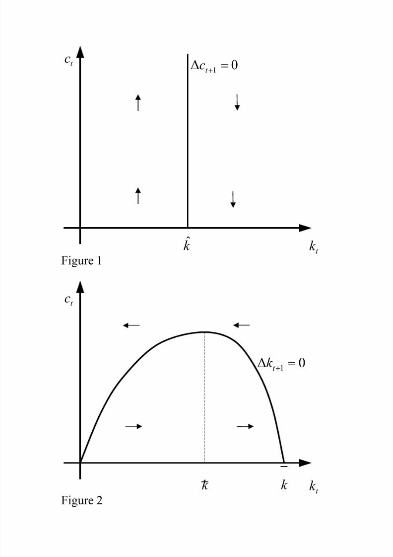
8/15/2019 Feminis
http://slidepdf.com/reader/full/feminis 75/82
0∆ 1 =+t ct
c
t k k
Figure 1
0∆ 1 =+t k
t c
t k k k Figure 2
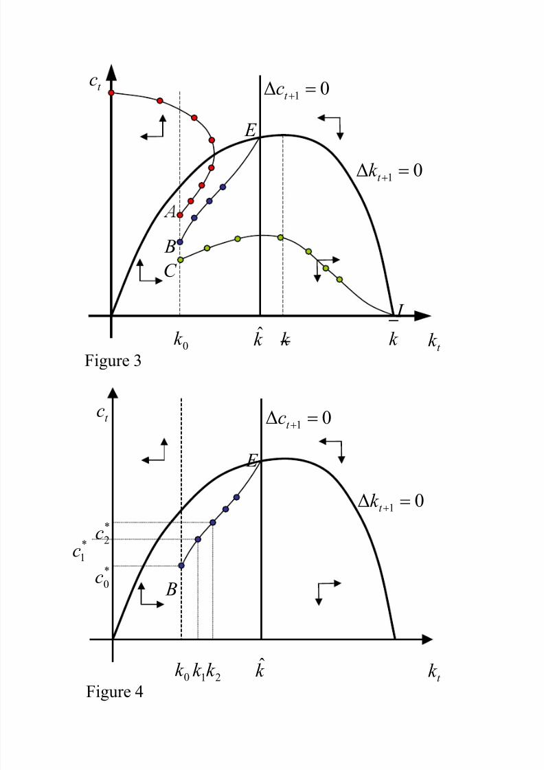
8/15/2019 Feminis
http://slidepdf.com/reader/full/feminis 76/82
0∆ 1 =+t ct
c
t k k
0∆ 1 =+t k
0k
I
E
B
C
Figure 3
k k
t c
t k k 0k
E
B
*
0c
1k 2k
*
1c
*
2c
Figure 4
0∆ 1 =+t c
0∆ 1 =+t k

8/15/2019 Feminis
http://slidepdf.com/reader/full/feminis 77/82
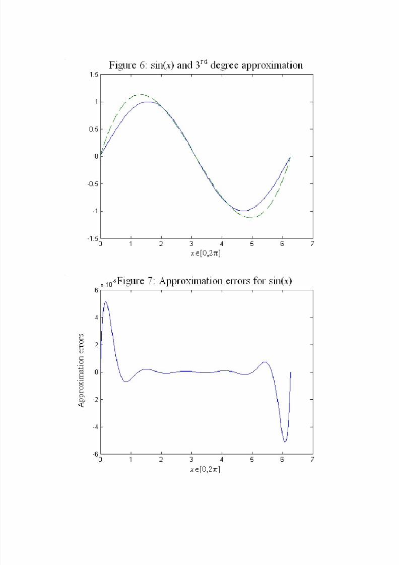
8/15/2019 Feminis
http://slidepdf.com/reader/full/feminis 78/82

8/15/2019 Feminis
http://slidepdf.com/reader/full/feminis 79/82

8/15/2019 Feminis
http://slidepdf.com/reader/full/feminis 80/82

8/15/2019 Feminis
http://slidepdf.com/reader/full/feminis 81/82

8/15/2019 Feminis
http://slidepdf.com/reader/full/feminis 82/82