female employment and fertility – the effects of …cep.lse.ac.uk/pubs/download/dp1156.pdfissn...
TRANSCRIPT

ISSN 2042-2695
CEP Discussion Paper No 1156
July 2012
Female Employment and Fertility - The Effects of
Rising Female Wages
Christian Siegel

Abstract Increases in female employment and falling fertility rates have often been linked to rising
female wages. However, over the last 30 years the US total fertility rate has been fairly stable
while female wages have continued to grow. Over the same period, we observe that women's
hours spent on housework have declined, but men's have increased. I propose a model with a
shrinking gender wage gap that can capture these trends. While rising relative wages tend to
increase women's labor supply and, due to higher opportunity cost, lower fertility, they also
lead to a partial reallocation of home production from women to men, and a higher use of
labor-saving inputs into home production. I find that both these trends are important in
understanding why fertility did not decline to even lower levels. As the gender wage gap
declines, a father's time at home becomes more important for raising children. When the
disutilities from working in the market and at home are imperfect substitutes, fertility can
stabilize, after an initial decline, in times of increasing female market labor. That parents can
acquire more market inputs into child care is what I find important in matching the timing of
fertility. In a mode l extension, I show that the results are robust to intrahousehold bargaining.
Keywords: Fertility, female labor supply, household production, intrahousehold allocations
JEL Classifications: D13, E24, J13, J22
This paper was produced as part of the Centre’s Macro Programme. The Centre for Economic
Performance is financed by the Economic and Social Research Council.
Acknowledgements I am grateful to Francesco Caselli, my advisor, and to Zsofia Barany, Wouter den Haan,
Monique Ebell, Ethan Ilzetzki, Rigas Oikonomou, Albert Marcet, Michael McMahon, Rachel
Ngai, Silvana Tenreyro, and seminar participants at the LSE for many comments and
suggestions.
Christian Siegel is an Occasional Research Assistant at the Centre for Economic
Performance, London School of Economics.
Published by
Centre for Economic Performance
London School of Economics and Political Science
Houghton Street
London WC2A 2AE
All rights reserved. No part of this publication may be reproduced, stored in a retrieval
system or transmitted in any form or by any means without the prior permission in writing of
the publisher nor be issued to the public or circulated in any form other than that in which it
is published.
Requests for permission to reproduce any article or part of the Working Paper should be sent
to the editor at the above address.
C. Siegel, submitted 2012
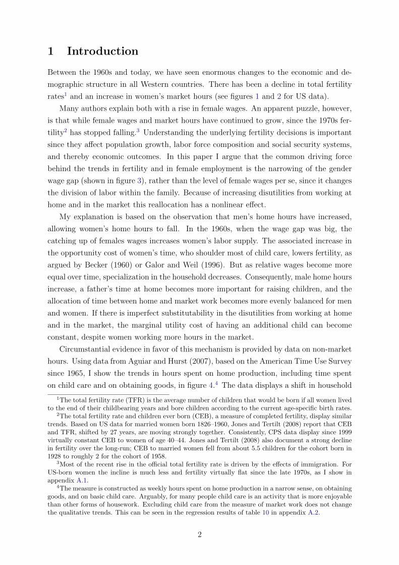
1 Introduction
Between the 1960s and today, we have seen enormous changes to the economic and de-
mographic structure in all Western countries. There has been a decline in total fertility
rates1 and an increase in women’s market hours (see figures 1 and 2 for US data).
Many authors explain both with a rise in female wages. An apparent puzzle, however,
is that while female wages and market hours have continued to grow, since the 1970s fer-
tility2 has stopped falling.3 Understanding the underlying fertility decisions is important
since they affect population growth, labor force composition and social security systems,
and thereby economic outcomes. In this paper I argue that the common driving force
behind the trends in fertility and in female employment is the narrowing of the gender
wage gap (shown in figure 3), rather than the level of female wages per se, since it changes
the division of labor within the family. Because of increasing disutilities from working at
home and in the market this reallocation has a nonlinear effect.
My explanation is based on the observation that men’s home hours have increased,
allowing women’s home hours to fall. In the 1960s, when the wage gap was big, the
catching up of females wages increases women’s labor supply. The associated increase in
the opportunity cost of women’s time, who shoulder most of child care, lowers fertility, as
argued by Becker (1960) or Galor and Weil (1996). But as relative wages become more
equal over time, specialization in the household decreases. Consequently, male home hours
increase, a father’s time at home becomes more important for raising children, and the
allocation of time between home and market work becomes more evenly balanced for men
and women. If there is imperfect substitutability in the disutilities from working at home
and in the market, the marginal utility cost of having an additional child can become
constant, despite women working more hours in the market.
Circumstantial evidence in favor of this mechanism is provided by data on non-market
hours. Using data from Aguiar and Hurst (2007), based on the American Time Use Survey
since 1965, I show the trends in hours spent on home production, including time spent
on child care and on obtaining goods, in figure 4.4 The data displays a shift in household
1The total fertility rate (TFR) is the average number of children that would be born if all women livedto the end of their childbearing years and bore children according to the current age-specific birth rates.
2The total fertility rate and children ever born (CEB), a measure of completed fertility, display similartrends. Based on US data for married women born 1826–1960, Jones and Tertilt (2008) report that CEBand TFR, shifted by 27 years, are moving strongly together. Consistently, CPS data display since 1999virtually constant CEB to women of age 40–44. Jones and Tertilt (2008) also document a strong declinein fertility over the long-run; CEB to married women fell from about 5.5 children for the cohort born in1928 to roughly 2 for the cohort of 1958.
3Most of the recent rise in the official total fertility rate is driven by the effects of immigration. ForUS-born women the incline is much less and fertility virtually flat since the late 1970s, as I show inappendix A.1.
4The measure is constructed as weekly hours spent on home production in a narrow sense, on obtaininggoods, and on basic child care. Arguably, for many people child care is an activity that is more enjoyablethan other forms of housework. Excluding child care from the measure of market work does not changethe qualitative trends. This can be seen in the regression results of table 10 in appendix A.2.
2

50
01
00
01
50
02
00
02
50
0
1970 1980 1990 2000 2010Year
Male Female
All Men and Women
50
01
00
01
50
02
00
02
50
0
1970 1980 1990 2000 2010Year
Male Female
Married
50
01
00
01
50
02
00
02
50
0
1970 1980 1990 2000 2010Year
Male Female
Single
PSID data
Yearly Hours Worked
Market Hours of Individuals Aged 20-60
Figure 1: Male and Female Market Hours Worked
1.5
22.5
3
1965 1975 1985 1995 2005Year
TFR US Born Women Offical TFR
Source: Vital Statistics of the United StatesOwn Calculations, using Population Estimates from US Census
Total Fertility Rate
Figure 2: Total Fertility Rate
3

.6.6
5.7
.75
.8
1965 1975 1985 1995 2005Year
Estimated Gender Wage Gap
Figure 3: Gender Wage Gap (see section 3.1)
production from women to men, with an overall reduction of hours worked at home. My
findings are consistent with the earlier work of Robinson and Godbey (2008), who find,
based on time use data for 1965 to 1995, that there is convergence in activities across
gender.5
The importance of considering intrahousehold allocations can be seen in the right
panels of figure 4. While home hours of married men have increased over time, single
men’s hours of home production are constant, after an initial change between 1965 and
1975. This is consistent with the explanation I propose. Single men, without a female
partner, are not affected by rising female wages, but married men spent more hours
working at home –a trend in US data that has not received much attention by researchers
yet, with the notable exception of Knowles (2007).6 Single women, on the other hand,
spend less time working at home, but the decline is not as pronounced as for married
women, whose husbands devote more of their time to home production.7
To the best of my knowledge, the only previous paper that has noted the flattening
out in total fertility rates and informally suggested an explanation in terms of increased
male home production is Feyrer et al. (2008). My paper formally models and quantifies
the endogenous response of male and female hours and their implications for fertility.8 I
5They also report that average parental hours spent on child-care per child has been roughly constant.Ramey and Ramey (2010), on the other hand, include time spent teaching children and document a risesince the mid 1990s, especially for college educated parents.
6Burda et al. (2007) study time use data across various developed countries, and find that total work,the sum of home and market work, is virtually the same for men and women. For the US, Ramey andFrancis (2009) report that total work of men and women has been constant throughout the 20th.
7In the Aguiar and Hurst (2007) data marital status is defined in a legal sense, and it is not possibleto disentangle cohabiting from other singles. In figure 19 of the appendix I show that home hours havechanged more for singles with children, who are more likely to be cohabiting, than for singles withoutchildren.
8Feyrer et al. (2008) explain the increase in male home hours with intrahousehold bargaining. I showthat bargaining is not necessary; a change in relative wages per se implies not only a reallocation of workin the market, but also at home. However, I also explore a version with intrahousehold bargaining.
4

10
20
30
40
50
1965 1975 1985 1995 2005Year
Male Female
All Men and Women
10
20
30
40
50
1965 1975 1985 1995 2005Year
Male Female
Married
10
20
30
40
50
1965 1975 1985 1995 2005Year
Male Female
Single
Data from Aguiar and Hurst (2007) - ATUS
Weekly Hours Spend on Non-Market Work and Basic Child Care
Non-Market Hours of All Men and Women Aged 20-80
Figure 4: Male and Female Home Hours Worked
present a general equilibrium model matching the observed patterns of fertility and hours
worked through an exogenous decrease in the gender wage gap. In the benchmark model
I consider households maximizing the sum of male and female members utilities. A rise
in female relative wages directly increases female labor supply and lowers female home
production, whereas male time is getting devoted more to home activities and less to
market work. Initially, when the gender wage gap is big, there is an overall drop in home
labor and a couple devotes less time to having and raising children. However, when the
gender wage gap is fairly small and shrinks further, the rise in male time spent working
at home is almost big enough to keep total home labor constant. The reason for this
differential reaction to improvement in female relative wages is in the increasing marginal
disutility from working. Initially, specialization in the household meant a husband’s labor
supply was much higher than his wife’s, and therefore he was less willing to spend more
time on home production. But as relative wages become more equal, the spouses time
allocation, and thus their disutilities from working, are getting closer to each other, and
in the limit a drop in female home production is fully offset by men. To the extent
that disutilities from market and home labor are imperfect substitutes, this reallocation
of hours worked can be consistent with the couple’s utility cost of child care remaining
constant. On top of this, with the improvement in the wife’s earnings, a couple can acquire
more parental time saving inputs. Both the rise in male home labor and the higher use
of parental time-saving inputs into home production is what I find key in explaining the
flattening out of the total fertility rate.
5

In a model extension I show that these results are robust to intrahousehold bargaining.
Calibrated against US data, my model suggests that for the trends in fertility changing
relative wages per se are much more important than their bargaining-induced shifts in
intrahousehold allocations.
Other papers that have studied the implications of the decline in the gender wage gap
for both male and female hours are Jones et al. (2003) and Knowles (2007), but none of
these papers has explored the implications for fertility. Galor and Weil (1996) present a
unified framework to explain the rise in female employment and the fall in fertility that
we observed until the mid 1970s. Since their mechanism links fertility decisions to the
market value of women’s disposable time9, it cannot explain why fertility stopped falling
when female wages continued improving. My model therefore highlights that the existing
literature that assumes perfect specialization within families, such that women shoulder
all of child care, has overlooked important implications of intrahousehold allocations.
2 The Model
2.1 Assumptions
I build a general equilibrium model of overlapping generations. Agents enter the economy
as young adults at age 20 and can have children in the first period of their lives, before
they turn 30. At age 60, agents retire, and they die deterministically at age 80. The
advantage of this modeling approach is that it incorporates an explicit age structure and
has implications for the demographic pyramid. Fertility leads to population growth and
thereby affects future labor markets and factor prices, and also social security benefits.
Moreover, I can feed in a life-cycle profile of wages which makes the model more realistic.
The complication with this approach is, I need to keep track of when children are born, as
this implies when they turn adults and leave their parent’s household. Thus, I assume for
tractability that each cohort can be represented by one representative household, formed
by a representative male and female, which can have a continuous number of children. Also
the length of the model period is motivated by tractability; a model period corresponds
to 10 years.
2.1.1 Agents and Households
All agents, men and women, derive utility from consumption of a market good (c) and
from having children (b), but derive disutility from working in the labor market (n) and
at home (h). They discount the future with factor β.
9Other papers linking fertility decisions to the market value of women’s disposable time include Green-wood et al. (2005) and Doepke et al. (2007).
6
Agents differ in terms of their gender (g ∈ {m, f}) and their age (j). I assume that all
economic active men and women live in couple households, formed by one man (‘husband’)
and one woman (‘wife’). Children live with their parents. In other words, when children
move out of their mother’s and father’s household, they find a spouse right away and
form a new couple household. To keep things simple I assume that both spouses are
of the same age and have the same deterministic life-span, which I denote by Tl. For
computational tractability, I assume that women, and hence couples, can have children
only in the first period of their (adult) life. I denote a couple’s total number of children
by b and the number of children living in their household by bh. I assume that children
leave the parental household after Ta periods. While parents derive utility from having a
child as long as they are alive themselves, households do not leave bequests, abstracting
from any further intergenerational altruism. Therefore agents start their economic-active
life (at age j = 1) with zero assets and leave no assets when they die (at age j = Tl).
Couples retire at age Tr, stop working in the market and receive social security benefits
Tss each period.
Let the absolute size of the cohort of couples of age j in period t be
St(j) (1)
In period t, the population share of the cohort aged j is then
µt(j) =St(j)Tl∑k=1
St(k)
(2)
I apply a model of collective household behavior, as introduced by Chiappori (1988). The
male and the female partner have their own preferences, and derive felicity um and uf
respectively. Since they hold wealth jointly and might have children together, they solve a
joint maximization problem. In particular, the couple household solves a Pareto program
with relative weight θ attached to the husband’s and 1 − θ to the wife’s utility. In the
benchmark model, the household behaves as a unitary agent and θ = 0.5 throughout.
For the model with household bargaining, I assume that the Pareto weight is determined
through Nash bargaining over the surplus generated by marriage, where the threat point
of a spouse is not entering the marriage (at age j = 1). To simplify the computations, I
assume full-commitment such that the weights –once determined– remain constant over
a household’s lifetime and there is no divorce. In general, the outcome of the bargaining
depends on each partner’s relative outside option of staying single. Life-time utilities of
single men and women differ to the extent that they face different wages. The outcome
of the bargaining therefore depends on relative wages, and the Pareto weight (θ) is a
function of the gender wage gap over the couple’s life-time ({χt+j−1}Tlj=1).
7

2.1.2 Fertility
Childbearing imposes a time-cost on the mother (τb), whereas child-care requires more
home production (x), which could be done by the father, the mother, or both.10. A further
input to home production are goods acquired in the market (e). Although I refer to this
home-labor saving input for simplicity as home appliances, in a more broader sense this
can also include paid domestic help, such as hiring nannies.
I assume that the amount of the home good needed is
x = x(bh) with x′(bh) > 0 (3)
Couples can have children only in the first period of their lives. Bearing a child reduces
the mother’s disposable time by τb in that period.
2.1.3 Household Production
Following Olivetti (2006) and Knowles (2007), I assume that the home good is produced
using a technology that is consistent with substitution among household member’s time
(h) and home appliances (e), which I model as a flow to simplify matters, according to
xh = eγH1−γ
where home labor input is
H = zmhm + zfhf
and zm and zf are the male and female home labor productivities, respectively.
A change in spouse’s relative wages will have an effect on market hours, home hours,
as well as on home appliances used. Rising market wages could lead to increases in market
hours and decreases in home hours –such as we have observed in the data for married
females–, without a drop in home production, as the household can acquire more home
appliances. In other words, the technology allows, to some degree, for a marketization of
inputs to home production11.
The home good is non-storable and is a public good within the household.
2.1.4 Market Technology
Assume there is a final goods technology of the form
Yt = AKαt N
1−αt (4)
10The former assumption is similar to Erosa et al. (2010), the latter is as in Knowles (2007) and similarto Greenwood and Seshadri (2005)
11In a structural transformation framework, Ngai and Pissarides (2008) study substitutions betweenhome and market production, but do not distinguish between male and female labor.
8
aggregating total market labor (N) and capital (K) into a final good which can be used for
consumption (c), investment in future capital stock, and for home appliances (e), which
I model as a flow to simplify matters. Capital depreciates at a rate δ each period.
The final goods sector is competitive. Factor prices are therefore equated to marginal
products, implying for the rental rate of capital (r) and wage rate per efficiency unit of
labor (w)
rt = αAKα−1t N1−α
t − δ (5)
wt = (1− α)AKαt N
−αt
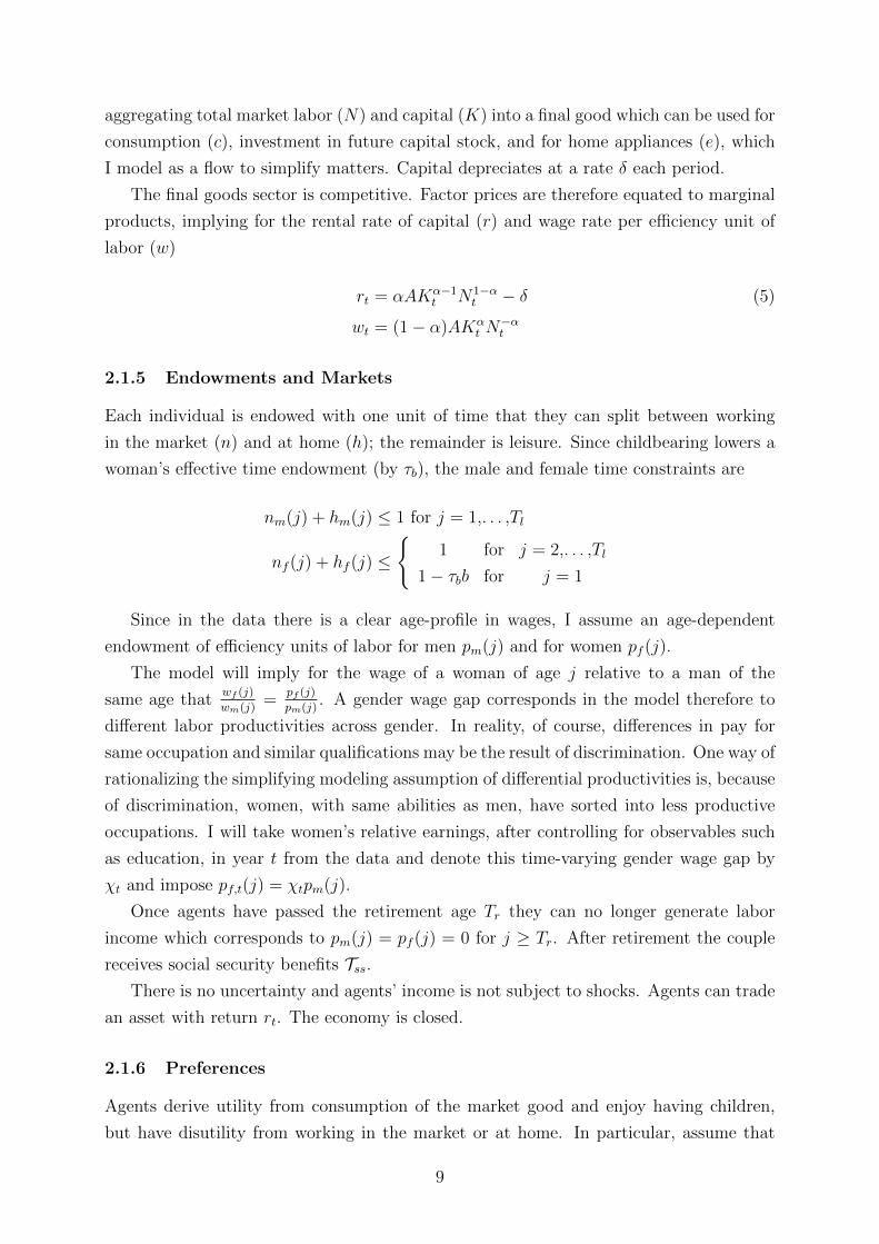
2.1.5 Endowments and Markets
Each individual is endowed with one unit of time that they can split between working
in the market (n) and at home (h); the remainder is leisure. Since childbearing lowers a
woman’s effective time endowment (by τb), the male and female time constraints are
nm(j) + hm(j) ≤ 1 for j = 1,. . . ,Tl
nf (j) + hf (j) ≤
{1 for j = 2,. . . ,Tl
1− τbb for j = 1
Since in the data there is a clear age-profile in wages, I assume an age-dependent
endowment of efficiency units of labor for men pm(j) and for women pf (j).
The model will imply for the wage of a woman of age j relative to a man of the
same age thatwf (j)
wm(j)=
pf (j)
pm(j). A gender wage gap corresponds in the model therefore to
different labor productivities across gender. In reality, of course, differences in pay for
same occupation and similar qualifications may be the result of discrimination. One way of
rationalizing the simplifying modeling assumption of differential productivities is, because
of discrimination, women, with same abilities as men, have sorted into less productive
occupations. I will take women’s relative earnings, after controlling for observables such
as education, in year t from the data and denote this time-varying gender wage gap by
χt and impose pf,t(j) = χtpm(j).
Once agents have passed the retirement age Tr they can no longer generate labor
income which corresponds to pm(j) = pf (j) = 0 for j ≥ Tr. After retirement the couple
receives social security benefits Tss.There is no uncertainty and agents’ income is not subject to shocks. Agents can trade
an asset with return rt. The economy is closed.
2.1.6 Preferences
Agents derive utility from consumption of the market good and enjoy having children,
but have disutility from working in the market or at home. In particular, assume that
9

preferences are additively separable and given by12
ug(c, n, h, b) =c1−σ − 1
1− σ−
(φn
(n1+η
1 + η
) s−1s
+ φh
(h1+ε
1 + ε
) s−1s
) ss−1
+ φbb1−σb − 1
1− σb(6)
These preferences feature imperfect substitutability of disutilities of working in the
market or at home. I view it as realistic to allow the utility cost of these two very different
activities to differ, but nonetheless there is a relationship between the two: The marginal
disutility of supplying an additional hour of market work is increasing in the time worked
at home, and vice versa. These preferences allow for time allocations, consistent with
the data, such that both men and women work in the labor market and in the household
–even when male and female time are perfect substitutes.
I assume that there is a subsistence level in consumption of the home produced good.
A household needs to produce a certain amount of the home good x, which is increasing
in the number of children living in the household (bh). As a simplifying assumption,
following Knowles (2007), agents do not derive any further utility from home production,
and this constraint will be binding, x = x(bh).
2.1.7 Government
The government provides a pay-as-you go social security system. Similar to the US system,
it levies a constant social security tax τss on labor income and redistributes the proceeds
as benefits Tss to retired households. Hence
Tss,t =τss · wtNt
Tl∑j=Tr
µ(j)
(7)
2.2 Couple Household’s Optimization
In the benchmark model I consider households in which spouses get equal weights (θ =
0.5), such that the household behaves like a unitary agent. Since I assume for the bargain-
ing model full commitment to the sharing rule determined when both partners meet (see
section 5.1), in both scenarios the Pareto weight θ is constant over the couple’s lifetime.
Consider the optimization problem of a couple household of age j with current wealth
a, total number of children b, of which bh are still living at home. Let ug(cg, ng, hg, b)
denote the own utility function of the member of gender g ∈ {m, f}. The household’s
resources from financial assets are a(1+r). Households before retirement can earn a labor
income net of taxes of wm(j)nm + wf (j)nf , where wm(j) = (1 − τss)pm(j)w is the net
12Adding utility from children in this additive form is generalizing Galor and Weil (1996) and Green-wood and Seshadri (2005), who assume simply ln(b).
10

male wage and wf (j) = χwm(j) the net female wage. After reaching the retirement age
(Tr) households receive social security benefits Tss.After having decided at the beginning of their lives on the number of children (b), for
age j ≥ 2 the value functions of the representative couple household solves13
VC(a; b, j) = maxa′,e,cm,cf
nm,nf ,hm,hf
θum(cm, nm, hm, b) + (1− θ)uf (cf , nf , hf , b) +βVC(a′; b, j+ 1) (8)
subject to the constraint set:
a′ =
{(1 + r)a+ wm(j)nm + wf (j)nf − cm − cf − e for j < Tr
(1 + r)a+ Tss − cm − cf − e for j ≥ Tr(9)
x(bh) = eγ (zmhm + zfhf )1−γ (10)
bh(j) =
{b for 1 ≤ j < Ta
0 for j > Ta(11)
nm + hm ≤ 1 and nf + hf ≤ 1 (12)
VC(·;Tl + 1) = 0 and aTl+1 = 0 (13)
{wm(k), wf (k), r(k)}Tlk=j known (14)
In the first period of a household’s life, the value function is different. Then the couple
decides on the number of children (b), from which the parents will derive utility throughout
their lifetime. Since I am focusing on a representative couple, the household can choose
any non-negative continuous quantity. At model age j = 1, when the household starts
out and is without any assets (a = 0), the value function solves
VC(0; b; 1) = maxb,a′,e,cm,cfnm,nf ,hm,hf
θum(cm, nm, hm, b) + (1− θ)uf (cf , nf , hf , b) + βVC(a′; b; 2) (15)
subject to the constraints (9) to (14), with the female time constraint (12) modified to be
nm + hm ≤ 1 and nf + hf ≤ 1− τbb (16)
since having children lowers the mother’s disposable time.
There is no closed form solution to this optimization problem, but the usual Euler
equations hold. Numerically, I solve a couple’s deterministic finite life-time optimization
problem (8) conditional on a fertility history backwards, making use of the intratemporal
first-order conditions, which I show in the appendix. Then I choose the number of children
that maximizes the couple’s life-time value function in the first period of their lives (15).
13To economize on notation, I do not index variables by time, but it should be understood that age (j)takes on this intertemporal role.
11

The optimal choice of number of children b is –off corners– such that
φbb−σb
Tl∑j=1
βj−1 =θ
γ
Ta∑j=1
βj−1cm(j; b)−σ(
x(b)
zmhm(j; b) + zfhf (j; b)
) 1−γγ
x′(b) (17)
=θ
zm
Ta∑j=1
βj−1
(φn
(nm(j; b)1+η
1 + η
) s−1s
+ φh
(hm(j; b)1+ε
1 + ε
) s−1s
) 1s−1
φhhm(j; b)ζ x′(b)
=1− θzf
Ta∑j=1
βj−1
(φn
(nf (j; b)
1+η
1 + η
) s−1s
+ φh
(hf (j; b)
1+ε
1 + ε
) s−1s
) 1s−1
φhhf (j; b)ζ x′(b)
where φh = φh(1 + ε)1/s and ζ = (s−1)ε−1s
.
Intuitively, when choosing a fertility plan the couple is outweighing benefits and costs
from having children. The marginal benefit of having this extra child arises from higher
felicity for the rest of couple’s lifetime, the left-hand side of (17). The marginal cost of
having more children lies in the need for more home production, for as long as the child
lives with the parents (Ta periods). To increase home production, the couple devotes
more time to home labor and uses more home appliances. Both adjustments reduce
consumption of the parents. As male and female home labor rises, the parents find it more
costly to supply as much labor to the market, and therefore generate less income. Since
home appliances are acquired in the market, disposable income for goods consumption
drops further. This marginal cost to the parents is, when time constraints are slack, the
right-hand side of (17). If a mother’s time constraint was binding, the time cost of having
the baby would have a further effect of lowering consumption, since she would have less
time to divide between market work and home production and loses earnings potential
(τbwf ).
2.3 Equilibrium
An equilibrium is an allocation of prices and quantities such that all couple households
are optimizing life-time utility, the representative firm maximizes profits, the government
budget balances, all market clears, and population growth is determined by past fertility
decisions. In particular, factor prices are determined competitively by (5), government
budget balances requires for social security (7), and households of all ages solve their
optimization problem (8) and (15), including the bargaining (31) when the household is
12

formed. Moreover, factor markets clear according to14
Nt =Tr∑j=1
St(j) (pmnm,t(j) + pf (j)nf,t(j)) (18)
Kt =
Tl∑j=1
St(j)at(j) (19)
and the size of cohorts of adult couples is given by
St(j) =
12St−Ta(1)bt−Ta for j = 1
St−1(j − 1) for 2 ≤ j ≤ Tl
0 for j > Tk
(20)
On the right hand side the shift of Ta periods appears since children turn adult after
Ta periods and have been born when their parents where of age j = 1. The factor 1/2
in front reflects the fact that children born are half boys and half girls, and a couple
household consist of a man and a woman (of the same age). Notice that in this model the
population growth rate might change over time, which in turn affects the capital-labor
ratio.
The model implies for period t a working-age average male and female labor supply of
Nm,t =
TR−1∑j=1
µt(j)nm,t(j) (21)
Nf,t =
TR−1∑j=1
µt(j)nf,t(j) (22)
where µt(j) = µt(j)/(∑TR−1
k=1 µt(k))
is the mass of the aged j cohort relative to the
working-age population. Similarly, average (over all ages) home hours and appliances are
Hm,t =
Tl∑j=1
µt(j)hm,t(j) (23)
Hf,t =
Tl∑j=1
µt(j)hf,t(j) (24)
Et =
Tl∑j=1
µt(j)et(j) (25)
14I solve for the equilibrium using a Auerbach and Koltikoff (1987) type algorithm. This entails 1.guessing time-paths for aggregate state variables and thereby of factor prices, 2. solving the optimizationproblems of all households given the guesses, 3. aggregating over all generations alive and computing thedeviations from the guessed paths, 4. If the deviations are sufficiently small, the equilibrium has beenfound; if not, update the guesses and iterate until consistent.
13

Since couples can have children only at the beginning of their adult lives, the total fertility
rate in period t is simply given by the number of children the representative household of
model age j = 1 has in that period
TFRt = bt (26)
3 Calibration
I choose parameters such that the model replicates in a base year the total fertility rate
and married male and married female hours worked, both at home and in the market. I
calibrate all parameters as time-invariant, and the only exogenous change over time is in
the gender wage gap. A model period is set to 10 years. I calibrate the model parameters
against data for 1965, taking the demographic structure of that year, the size of cohorts
and the population growth rate, as given. For the required amount of home production,
I make use of the cross-sectional variation of married men’s and women’s hours against
the number of children in the household. table 1 lists all model parameters, along with a
value taken from the literature15, or whether it is to be set in a calibration exercise.
In the literature the range of estimates of the labor share in home production is very
wide. Studies that include housing as capital or equipment used for home production
typically find a relatively low value, close to the one of market production, e.g. Greenwood
et al. (1995), while Benhabib et al. (1991), who exclude housing, estimate a very high
value of 0.92. In my model, the need for home production is at the margin entirely arising
from having children living in the household, and does not correspond closely to either
study. Since parents can acquire home production inputs in the market, such as hiring
nannies or paid domestic help, the share of time-saving inputs acquired in the market, γ,
should be higher than the Benhabib et al. (1991) value. As a benchmark I consider an
intermediate value of γ = 0.2, but I conduct a series of robustness checks, see section 7.
3.1 The Gender Wage Gap as Ratio of Residual Wages
To construct a series of the gender wage gap to feed into the model, I use data from the
Panel Study of Income Dynamics (PSID) for the United States from 1968 to 2007.16First
I regress for individuals aged 20 to 59 the logarithm of real wages on a set of observables,
15As an approximation to the first order, the Frisch elasticity of market labor supply –when time-constraints are slack– is 1
η .16In section A.4 of the appendix, I discuss the advantages of using data from the PSID, rather than
from the CPS, and compare the data and results from these two surveys.
14

Description Value/Moment to Match
Preference Parametersσ elasticity of consumption 1 (log-utility)σb elasticity of demand for children calibrationη related to elasticity of market hours 2 (Domeij and Floden (2006))ε related to elasticity of home hours calibrations CES elasticity of disutilities to work calibrationφn weight on disutility market labor calibrationφh weight on disutility home labor calibrationφb weight on utility from children calibrationβ discount factor 0.94710 (Cooley and Prescott (1995))
Market Technologyα capital share in market output 0.36 (Hansen (1985))A total factor productivity 1 (normalization)δ depreciation of capital 1− (1− 0.047)10 (Cooley and Prescott (1995))pm(j) male wage profile estimated, see section 3.1τss social security tax rate 11% (Heer and Maußner (2009))
Home Technologyγ share of market inputs in home 0.2 (and robustness checks)zm male home labor productivity 1 (normalization)zf female home labor productivity 1 (assuming zm = zf )τb time cost on mother per child 1
2110
(6 month)x(bh) amount of home good needed cross-sectional variation
Time Variantχt gender wage gap estimated, see section 3.1
Table 1: Model Parameters
15

including most importantly education. In particular I estimate by OLS
logwi,t = β0,t + β1,tDfemalei,t + L(j) +Xi,tγ + εi,t (27)
where Dfemalei,t =
{1 if i is female
0 if i is male
L(j) is a polynomial in age
Xi,t is a vector of other observables, such as a polynomial
in years of education and race dummies
The estimated gender wage gap for year t, defined as the ratio of women’s to men’s
relative earnings not explained by Xi,t, is then given by eβ1,t . I give the full regression
results in appendix C.1, and plot the implied series in figure 3. To construct the series
of χt to feed into the model, where a period has a length of 10 years, I take the simple
averages.17 For the final steady state I assume that the gender wage gap is closed. I
impose for the transition periods between the last available data point and the steady
state, that χt grows at the same rate as over 1968–2007 until it reaches 1.
The estimates of equation 27 imply an age profile in wages, for male wages pm(j) =
exp(L(j)), which I illustrate in figure 5. Then I impose for females
pf,t(j) = χtpm(j) (28)
where I obtained χt as described above.
2.5
33.5
44.5
20 30 40 50 60Age
Age Profile of Wages
Figure 5: Age Profile of Wages
17As an alternative, I allow the gender wage gap to depend on time and age of the worker. Thequalitative results do not change; see appendix E.
16

3.2 Home Production
To calibrate the required amount of home goods x(bh), notice that the model implies
that male and female home and market hours depend on the couple’s Pareto weights,
consumptions and the required amount of home good x(bh). In particular, at an interior
solution the household’s first order condition imply
x(bh) =
φhφn
(1 + ε
1 + η
)1/sh
(s−1)ε−1s
m
n(s−1)η−1
sm
wmzm
γ
1− γ(zmhm + zfhf )
γ
(29)
Conditional on all other parameters, this relationship can be used to back out of x(bh)
from the Aguiar and Hurst (2007) data, based on the American Time Use Survey. As a
functional form I assume
x(bh) = κ0 + κ1 · bκ2h (30)
and expect to find κ0 > 0, κ1 > 0 and 0 < κ2 < 1, which would mean home production is
always positive and increasing in number of children, but at a decreasing rate. I choose
the parameters κ0, κ1, κ2 to replicate the observed cross-sectional variation of married
men’s and women’s hours against the number of children in the household, according to
(29). The details are given in appendix C.2.
3.3 Remaining Parameters
1965-Moments to be Matched Data Fictive S.S. in TransitionNumber of children (TFR) 2.913 2.9726 2.8493Market hours of men 0.3886 0.3890 0.3907Market hours of females 0.1120 0.1111 0.1139Home hours men 0.0950 0.0950 0.0953Home hours females 0.3896 0.3909 0.3893
Additional Target to be MatchedLong-run TFR 2 (assumed) 2.0312
For the 1965 moments, the first column shows the value of the statistics in the data. Thesecond column shows the model analogues, taking the demographics as given, when agentsbelieve the gender wage gap to remain constant forever. The third column shows the modelimplied outcomes, when in 1965 agents learn the true future path of the gender wage gap. Todiscipline the calibration a restriction on the long-run number of children is added. For thelong-run TFR, the last column shows the model’s final steady state TFR.
Table 2: Calibration Targets
Six parameters are left to be chosen, but I have only the five targets of table 2 to
match in 1965, the base year. Four parameters (φn, φh, ε, s) correspond to the targets for
male and female hours worked at home and in the market, and two parameters (φb, σb)
are key for the fertility choice.
17

These parameters are, of course, calibrated jointly, but it is insightful to think of them
as being chosen to match particular moments in the data. Notice that the optimality con-
ditions for a household before retirement imply(hm(j)hf (j)
) (s−1)ε−1s
= zmzfχ(j)
(nm(j)nf (j)
) (s−1)η−1s
.
Intuitively, given the gender wage gap and relative home productivities, s is chosen to
replicate the ratio of female to male labor supply. Then ε is set to match relative home
hours. Then φn and φh are chosen so that absolute male and female market and home
hours, respectively, equal the observed ones. Given these parameters, the cross-sectional
variation in hours worked against the number of children gives, according to (29), the pa-
rameters κ0, κ1, κ2, describing the required amount of home production x(bh). Finally, the
two parameters governing fertility have to be chosen. While φb captures the relative weight
the household attaches to having children (compared to consumption), σb essentially cap-
tures the curvature. I restrict the calibration by choosing σb such that in the final steady
state, the total fertility rate is approximately 2. A value of 2 seems natural, as the number
of children born is just replacing previous generations. Moreover, it is close to most recent
values for the US. Conditional on a value for σb, I calibrate the remaining five parameters
to the data of 1965 under the fiction that households believed gender wage gap to remain
constant forever. Then I solve the model for the final steady state, in which the gender
wage is closed. If the implied long-run fertility rate differs from 2, I update the guess
for σb until consistent. Table 3 shows the values found through this calibration exercise.
They imply for the required amount of home production x(bh) = 0.1813+0.0279(bh)0.8845.
Description Value
σb elasticity of demand for children 0.3950ε related to Frisch elasticity of home hours 3.5740s CES elasticity of disutilities to work 1.4041φn weight on disutility from market labor 2.6712φh weight on disutility from home labor 1.8398φb weight on utility from children 0.0515
Table 3: Calibrated Parameters
I perform a series of robustness checks, including alternative values for σb (and therefore
of φb), and report the model results under alternative parameters in section 7.
4 Results of the Benchmark Model
To obtain the transition path of the calibrated model, I feed the series of the observed
gender-wage gap into the model. For the first period I need initial conditions. I take the
demographic structure from the data. Since I do not have age-specific data on household
asset holdings for 1965, I initialize household asset holdings with the values of a fictive
18

1 2 3 4 5 6-0.1
-0.05
0
0.05
0.1
0.15
0.2
0.25Couple's Assets
1 2 3 4 5 60
0.5
1
1.5
2
2.5
3
3.5Children at Home
1 2 3 4 5 60
0.1
0.2
0.3
0.4
0.5
0.6
Labor Supply
Male
Female
1 2 3 4 5 60
0.1
0.2
0.3
0.4
0.5
0.6
Home Hours
Male
Female
This graphs plots the representative couple household’s policy functions for assets, male andfemale market and home hours, as well as number of children living at home, over the life-cycle,from age j = 1 (20–29) to j = Tl = 6 (70–79).
Figure 6: Life-time Choices in the Initial Steady State
steady state in which agents believed the gender wage gap to remain constant forever.18
It should be stressed that in the model young couples, who are the ones deciding on
how many children to have, start out with zero assets. The initialization of asset holdings
applies to older households only, and could affect fertility only through general equilibrium
effects on wages or interest rates, which are likely to be small.
I assume that the economy will eventually reach a steady state in which male and
female wages are equalized. Since fertility is a choice in the model, the age distribution
evolves endogenously over time. Like Auerbach and Koltikoff (1987), I select the long-
run equilibrium such that in the final steady state the growth rate of the population is
constant. A constant number of children per couple is not enough to ensure this outcome,
as an infinite echoing series of baby booms or busts might occur. Since a balanced growth
path requires constant population growth to ensure a constant capital-labor ratio, I solve
for the final steady state by solving a fixed-point problem for the population growth rate.19
19

4.1 Comparing the Steady States
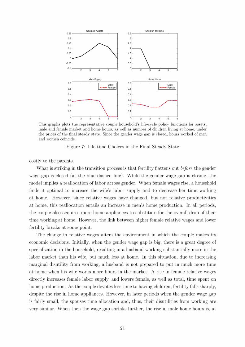
Figures 6 and 7 show the policy functions of the representative couple in the initial and in
the final steady state. In the initial steady state a couple has more than two children and
there is population growth. Therefore, there are relatively more young households in the
economy, who start out without any assets. As a consequence, the equilibrium interest
rate is such that β(1 + r) > 1, and consumption, both male and female, is increasing
over the household’s life-cycle. As consumption rises, an agent prefers to work less at a
given wage. However, holding consumption and home production constant, labor supply
increases in the wage rate. Since there is the age premium in wages (figure 5), these two
effects work against each other, resulting in the labor supply plotted in the graph.
In the initial steady state, the positive gender wage gap implies gains from specializa-
tion in the couple household. Consequently, a wife shoulders most of the housework, and
most of a couple’s labor supply is coming from the husband. In the final steady state, on
the other hand, the gender wage gap is closed, and there are no gains from specialization
anymore.20 Hours worked of men and women are therefore equalized, both in the market
sector and at home.
Comparing the policy functions of the final and the initial steady state shows, most
of the increase in female labor supply comes from young women, which is consistent with
the empirical findings by Buttet and Schoonbroodt (2006) and Olivetti (2006).
4.2 The Transition in the Benchmark Model
Figure 8 shows the transitional dynamics of the economy21, starting from an initial sit-
uation (t < 0), in which wages were expected to remain constant at their 1965 values.
Then at t = 0, corresponding to the year 1965, the true path of the gender wage gap gets
known, but relative wages do not start changing before t = 1, year 1975. The economy
starts to converge to a new steady state in which relative wages are equalized. During
the transition the gender wage gap, shown in the upper-left panel, closes gradually. As a
consequence, women work more hours in the market and less at home, whereas for men
the opposite happens. Initially, fertility is declining as raising children becomes more
18This is the fictive steady state used for calibrating the model against the data. The age-distributionof 1965 is, however, not the stationary distribution, which would be implied by the population growthrate of this year.
19First I guess a population growth rate, which implies a stationary age distribution. Then I computethe steady state. In particular, the optimally chosen number of children, compared to the measure ofoldest households gives an implied population growth rate, according to (20). I iterate to find the fixedpoint.
20By assumption male and female home productivities are equal throughout. Advances in technologiesover the last century, such as infant formula, have brought male and female productivities closer together.Albanesi and Olivetti (2007) argue that this allowed female labor force participation to rise. In myframework, it also implies a rise in male participation at home.
21The transitional graphs in the main text show, in the interest of brevity, only the behavior of aggregatevariables. Section D of the appendix shows the disaggregation by age.
20
1 2 3 4 5 6-0.1
-0.05
0
0.05
0.1
0.15
0.2
0.25Couple's Assets
1 2 3 4 5 60
0.5
1
1.5
2
2.5
3
3.5Children at Home
1 2 3 4 5 60
0.1
0.2
0.3
0.4
0.5
0.6
Labor Supply
Male
Female
1 2 3 4 5 60
0.1
0.2
0.3
0.4
0.5
0.6
Home Hours
Male
Female
This graphs plots the representative couple household’s life-cycle policy functions for assets,male and female market and home hours, as well as number of children living at home, underthe prices of the final steady state. Since the gender wage gap is closed, hours worked of menand women coincide.
Figure 7: Life-time Choices in the Final Steady State
costly to the parents.
What is striking in the transition process is that fertility flattens out before the gender
wage gap is closed (at the blue dashed line). While the gender wage gap is closing, the
model implies a reallocation of labor across gender. When female wages rise, a household
finds it optimal to increase the wife’s labor supply and to decrease her time working
at home. However, since relative wages have changed, but not relative productivities
at home, this reallocation entails an increase in men’s home production. In all periods,
the couple also acquires more home appliances to substitute for the overall drop of their
time working at home. However, the link between higher female relative wages and lower
fertility breaks at some point.
The change in relative wages alters the environment in which the couple makes its
economic decisions. Initially, when the gender wage gap is big, there is a great degree of
specialization in the household, resulting in a husband working substantially more in the
labor market than his wife, but much less at home. In this situation, due to increasing
marginal disutility from working, a husband is not prepared to put in much more time
at home when his wife works more hours in the market. A rise in female relative wages
directly increases female labor supply, and lowers female, as well as total, time spent on
home production. As the couple devotes less time to having children, fertility falls sharply,
despite the rise in home appliances. However, in later periods when the gender wage gap
is fairly small, the spouses time allocation and, thus, their disutilities from working are
very similar. When then the wage gap shrinks further, the rise in male home hours is, at
21

0 10 200.5
0.6
0.7
0.8
0.9
1
1.1Female Relative Wages
0 10 20
1
1.5
2
2.5
3
3.5
TFR
0 10 200.009
0.0095
0.01
0.0105
0.011
0.0115
0.012Home Appliances
0 10 200
0.1
0.2
0.3
0.4
0.5Labor Supply
Male
Female
0 10 200
0.1
0.2
0.3
0.4
0.5Home Hours
Male
Female
0 10 200.2
0.4
0.6
0.8
1
1.2Factor Prices
w
r
This graphs shows the benchmark model’s transition over time, that is implied by the narrowingof the gender wage gap (upper-left panel). The dotted lines show the data, which is availableuntil 2005 (t = 5) only.
Figure 8: Transition Path of the Unitary Model (θ = 0.5)
22

a given level of home production, i.e. number of children, almost big enough to keep total
home labor constant; in the limit of equalized wages, a drop in female home production
is fully offset by men. On top of this, with the improvement in the wife’s earnings, the
couple can acquire more parental time saving inputs.
For the optimal choice on how many children to have, however, the couple outweighs
the benefits from having an additional child with the utility cost of child care. The
reallocation of a man’s time from market to home, which comes with the change in relative
wages, might actually reduce his marginal cost of having an additional child, although
his share of child care rises, since the disutilities are imperfect substitutes and his initial
time allocation was very unbalanced. Similarly, a mother’s marginal cost might increase,
fall, or not be affected at all. The model results clearly suggest that for the first part
of the transition, as female relative wages improve, the parents’ marginal utility cost is
increasing, and therefore they prefer to have fewer children. But when the gender wage
gap is sufficiently small and shrinks further, their marginal cost is not affect, resulting in
a constant fertility rate.
I will show in the next two sections that key in understanding why fertility did not
fall further is the rise in male home labor, that we have observed in the data. While
qualitatively the rise in male participation in home production can yield a flattening
out of the fertility rate, I find that the higher use of parental time-saving inputs into
home production is important in matching the timing. However, a marketization of home
production alone is not sufficient to explain the data.
4.3 Counterfactual: The Absence of Male Home Labor
In this part I am shutting down the rise of male home labor. In the existing literature
on fertility it is commonly assumed that child-care is a function of female time only. By
setting male home productivity to zero, my model nests this as a special case. Notice
that in this counterfactual exercise, men and women do not become ‘identical’ in the
final steady state. Although their wages will eventually be equalized, specialization in the
household persists because of the different home productivities.
Not to confound changes in technology with changes in preferences, I keep all pref-
erence parameters at their baseline values, but set zm = 0 and adjust zf such that the
household still chooses in 1965 the same number of children as in the data.22 Figure 9
shows the transition of the model, when men cannot counteract the fall in women’s home
hours.
It implies a monotone drop in fertility as long as female wages catch up– which is
inconsistent with the data. Throughout the transition, parents are having fewer and
22Since by assumption of zm = 0 this model variant is doomed to fail along the dimension of malehome hours, notice that I could not apply the calibration strategy of the benchmark model, which hasHm as one of the targets.
23

0 10 200.5
0.6
0.7
0.8
0.9
1
1.1Female Relative Wages
0 10 20
1
1.5
2
2.5
3
3.5TFR
0 10 200.01
0.011
0.012
0.013
0.014
0.015Home Appliances
0 10 200
0.1
0.2
0.3
0.4
0.5Labor Supply
Male
Female
0 10 200
0.1
0.2
0.3
0.4
0.5Home Hours
Male
Female
0 10 200.2
0.4
0.6
0.8
1
1.2Factor Prices
w
r
For the model without male home production, this graphs plots the transition implied by thenarrowing of the gender wage gap (upper-left panel) over time. The dotted lines show thedata, which is available until 2005 (t = 5) only.
Figure 9: Transition Path of the Unitary Model (θ = 0.5) with zm = 0
24

0 10 200.5
0.6
0.7
0.8
0.9
1
1.1Female Relative Wages
0 10 20
1
1.5
2
2.5
3
3.5
TFR
0 10 200.009
0.01
0.011
0.012
0.013
0.014
0.015Home Appliances
0 10 200
0.1
0.2
0.3
0.4
0.5Labor Supply
Male
Female
0 10 200
0.1
0.2
0.3
0.4
0.5Home Hours
Male
Female
0 10 200.2
0.4
0.6
0.8
1
1.2
1.4
1.6Factor Prices
w
r
For model without male home production under the alternative calibration, this graphs plotsthe transition implied by the narrowing of the gender wage gap (upper-left panel) over time.The dotted lines show the data, which is available until 2005 (t = 5) only.
Figure 10: Transition of the Unitary Model (θ = 0.5) with zm = 0, Alternative Calibration
fewer children, since child-care hours continue to fall, when women’s market labor supply
rises. As women’s income increase, couples also acquire more home appliances, but this
marketization of home production is not strong enough to prevent fertility from falling.
Only once the gender wage gap has closed, the optimal number of children stabilizes.
4.3.1 Alternative Calibration of the Model without Male Home Production
As an alternative calibration for the zm = 0-model, I adjust the parameters capturing
the choice of number of children, such that also this model variant has a total fertility
rate of 2 in the final steady state. More specifically, I take the benchmark calibration,
with zm = 0 and zf = 1, and adjust (φb, σb) to target a long-run TFR of 2, but keeping
1965’s TFR at the observed value. Given all other parameters from the benchmark, this
adjustment yields φb = 0.0872 and σb = 0.9625. Then I solve for the transition of the
model under this alternative calibration and show the results in figure 10. Also under
these alternative parameters, the model without male home production predicts that the
total fertility rate falls as long as the gender wage gap shrinks. That parents use more
market inputs into home production is not sufficient for generating a flattening out of the
fertility rate before the gender wage gap has closed.
25

To conclude, in the benchmark model of above, it is the rise in male home labor, which
counteracts the fall of female time inputs into child raising, that is key in understanding
why the fertility decline ended.
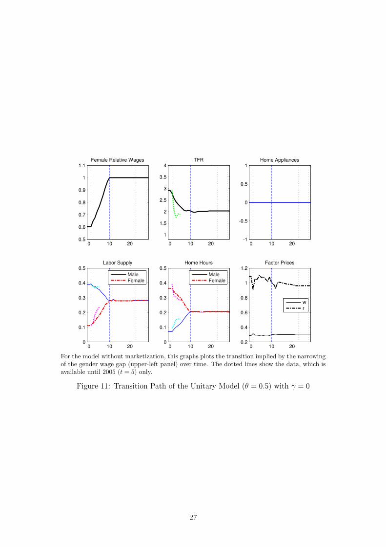
4.4 No Marketization of Home Production
Since the previous section concludes that the rise in male home production is important
in understanding why fertility did not fall further, one might wonder whether the mar-
ketization of home production matters for the trends in fertility after all. As I show in
this section, that parents can use more time-saving inputs at home when female wages
rise, is not crucial for replicating the flattening out of the total fertility rate qualitatively.
However, it is important in matching the timing.
To rule out marketization of home production, consider a simpler version of the model
in which home production is a function of male and female home hours only. This is the
special case of γ = 0. I use the same calibration strategy as for the benchmark model, in
order to give both models equal chances in matching the data.23
Figure 11 shows the transition of this model variant. Also the model without marketi-
zation predicts that fertility stops falling before the gender wage gap is closed (in t = 10,
at the dashed line). This shows that the reallocation of men’s time from market to home,
and of women’s time from home to the labor market is, in principle, sufficient in breaking
the direct link between higher female wages and fewer children. However, this version of
the model predicts that fertility does not flatten out before the year 2025 (t = 7), but in
the data the fertility rate has been constant already since the late 1970s. The benchmark
model featuring marketization of home production, on the other hand, gets closer and
predicts, as shown in figure 8, a flat fertility rate since 1995 (t = 4). In section 6, below,
I compare the different versions of the model and the data in greater detail.
23The same calibration strategy as for the benchmark model gives the following parameters:σb = 0.750, ε = 3.4935, s = 1.4073, φn = 2.6281, φh = 1.8434, φb = 0.0524 implying x(bh) =
0.3762 + 0.0515(bh)0.9254. They imply for the targets:
1965-Moments to be Matched Data Fictive S.S. in TransitionNumber of children (TFR) 2.913 2.9134 2.7982Market hours of men 0.3886 0.3890 0.3949Market hours of females 0.1120 0.1104 0.1159Home hours men 0.0950 0.0711 0.0715Home hours females 0.3896 0.3630 0.3616
Additional Target to be MatchedLong-run TFR 2 (assumed) 2.0279
26
0 10 200.5
0.6
0.7
0.8
0.9
1
1.1Female Relative Wages
0 10 20
1
1.5
2
2.5
3
3.5
4TFR
0 10 20-1
-0.5
0
0.5
1Home Appliances
0 10 200
0.1
0.2
0.3
0.4
0.5Labor Supply
Male
Female
0 10 200
0.1
0.2
0.3
0.4
0.5Home Hours
Male
Female
0 10 200.2
0.4
0.6
0.8
1
1.2Factor Prices
w
r
For the model without marketization, this graphs plots the transition implied by the narrowingof the gender wage gap (upper-left panel) over time. The dotted lines show the data, which isavailable until 2005 (t = 5) only.
Figure 11: Transition Path of the Unitary Model (θ = 0.5) with γ = 0
27
5 The Bargaining Model
Since Feyrer et al. (2008) have argued that changes in women’s household status is impor-
tant in explaining the time series in total fertility, I introduce next household bargaining.
The only modification to the benchmark model is that now the Pareto weights in the
household’s optimization program are determined endogenously.
Here, rising relative wages also improve women’s say in household decision making,
which corresponds in my model to a higher weight on women’s utility in a couple’s op-
timization program. I assume that this weight is the result of a Nash bargaining over
the surplus generated by marriage. The wife’s bigger say reduces her share of housework,
relative to her husband, by more than what a change in relative wages per se would imply.
5.1 Determination of Intrahousehold Weights
The solution to the couple’s optimization program at a given Pareto weight θ defines a
sequence of life-time utilities {VC,m(j|χ, θ), VC,f (j|χ, θ)}Tlj=1 for the man and the woman
who form the household. I follow McElroy and Horney (1981) and assume that the sharing
rule θ is the result of Nash Bargaining. When both partners meet at the beginning of their
adult lives, i.e. at model age j = 1, they bargain under full commitment over the surplus
generated from marriage. The threat point of each partner is staying single, rather than
entering the match. In equilibrium, the weights are then the solution to
θ = arg maxθ
[VC,m(1|χ, θ)− VS,m(1|χ)][VC,f (1|χ, θ)− VS,f (1|χ)] (31)
where VC,m(1|χ, θ) and VC,f (1|χ, θ) are the husband’s and wife’s lifetime utilities at age
j = 1 that are implied by the joint optimization program, and Vm,S(1|χ) and Vf,S(1|χ)
are the life-time utilities if the man or the women stayed single (at age j = 1), given the
series of the gender pay gap that they face over their lives (χ ={χj}Tlj=1 = { wf (j)wm(j)
}Tlj=1).
To find the value of the threat points, consider the optimization problem of male and
female singles. Since they cannot have children, the value function of a single agent of
28

gender g ∈ {m, f} solves
VS,g(a; j) = maxc,,n,h,e,a′
u(c, n, h, 0) + βVS,g(a′; j + 1) for j ≥ 1 (32)
subject to
a′ =
{(1 + r)a+ wg(j)n− c− e for j < Tr
(1 + r)a+ Tss2− c− e for j ≥ Tr
x(0) = eγH1−γ with H = zgh
n+ h ≤ 1
VS,g(·;Tl + 1) = 0 and a1 = Tl+1 = 0
{wg(k), r(k)}Tlk=j known
I find the singles’ value function at age j = 1 numerically. Then I solve the Nash
bargaining problem (31) to find a household’s Pareto weight. The resulting sharing rule
depends on the life-time series of the gender wage gap (θ = θ(χ)), since it changes the
outside option of females relative to males. In other words, the spouse’s bargaining
position depends on their relative wages. Typically the husband’s weight is increasing in
his relative life-time wages.
5.2 Dependence on the Weights
A rise in wives’ Pareto weights, relative to their husbands, –a drop in θ– makes them
better off through a intrahousehold reallocation of consumption and hours worked. One
optimality condition that is particular useful in illustrating the mechanism of the model
is the ratio of male to female home hours. When both time constraints (12) are slack, the
optimal division of home labor for retired couples is given by24
hmhf
=
(1− θθ
zmzf
)1/ε
for j ≥ Tr (33)
Increase in women’s relative Pareto weight imply an increase in the share of men’s
home hours. Numerically I find that this also the case for working-age couples. An
improvement in a woman’s bargaining position therefore decreases her share of home
hours and lowers her opportunity cost of having children. However, as her partner then
has to contribute more to home production, his preferred number of children is falling.
24One can show that as sl →∞, making the choice of home and market hours separable, the optimalitycondition (33) also holds for working-age couples.
29

5.3 Calibration
As for the benchmark model in section 3, I calibrate the model with intrahousehold
bargaining against data for 1965. I report the obtained parameter values in table 4, and
the targets and their counterparts in the model table 5. The calibrated parameters imply
for the required amount of home production x(bh) = 0.1923 + 0.0299(bh)0.8793.
Description Value
σb elasticity of demand for children 0.4800ε related to Frisch elasticity of home hours 4.1041s CES elasticity of disutilities to work 1.3673φn weight on disutility from market labor 2.3727φh weight on disutility from home labor 2.4044φb weight on utility from children 0.0764
Table 4: Calibrated Parameters for the Bargaining Model
1965-Moments to be Matched Data Fictive S.S. in TransitionNumber of children (TFR) 2.913 2.8371 3.0463Market hours of men 0.3886 0.3889 0.3941Market hours of females 0.1120 0.1111 0.1008Home hours men 0.0950 0.0948 0.0902Home hours females 0.3896 0.3885 0.4001
Additional Target to be MatchedLong-run TFR 2 (assumed) 2.0205
For the 1965 moments, the first column shows the value of the statistics in the data. Thesecond column shows the model analogues, taking the demographics as given, when agentsbelieve the gender wage gap to remain constant forever. The third column shows the modelimplied outcomes, when in 1965 agents learn the true future path of the gender wage gap. Todiscipline the calibration a restriction on the long-run number of children is added. For thelong-run TFR, the last column shows the model’s final steady state TFR.
Table 5: Calibration Targets for the Bargaining Model
5.4 Steady State Comparison
Table 6 shows the model implied variables for the 1965-steady state, taking the age
distribution as given, and the final steady state with endogenous distribution across age.
The steady state results of the bargaining model, rows 1 and 2, confirm, improvement in
women’s relative wages lead to a reduction in men’s Pareto weight in household decision
making. In the final steady state, in which the gender wage gap is assumed to have
disappeared, both spouses have an equal weight in the household optimization (θ = 0.5),
whereas initially, when men earned relatively more, husbands accrued a bigger weight.
Not surprisingly, in response to higher wages, female labor supply increases and
women’s share of home production decreases. Fertility is lower in the long run, when
30

χ µ(j) θ TFR Nm Nf Hm Hf
0.602 1965 data endogenous 0.612 2.8371 0.3889 0.1111 0.0948 0.38851.000 endogenous endogenous 0.500 2.0205 0.2972 0.2972 0.2254 0.2254
1.000 endogenous fixed at 0.612 2.0884 0.2407 0.3600 0.2351 0.2158
Table 6: Steady States Comparisons
the gender wag gap has closed. In the bargaining model there are three forces driving
fertility decisions. Firstly, higher wages exert a positive income effect increasing a couple’s
desire to have children. Secondly, higher relative earnings to women affect the division
of market and home labor between men and women. In particular, men have to con-
tribute more to home production, leaving women with more disposable time, which tends
to boost fertility. Thirdly, however, the bargaining effect has differential effects on men
and women. While a higher Pareto weight on females increases the number of children a
mother wants to have, it reduces the optimal number for men, who will need to provide
more input to child care.
To disentangle the effects, I conduct a counterfactual exercise. I vary women’s relative
wages, but keep the Pareto weights constant. The last row of table 6 shows the steady state
results under a fixed weight of θ = 0.612, which was found to be optimal under χ = 0.602.
Comparing them with the row above highlights the role of household bargaining: Under
my calibration, household bargaining reduces fertility in the final steady state. While the
improvement in women’s say in the household, which comes along with the shrinking of
the gender wage gap, increases their preferred number of children, it reduces the optimal
number of children for fathers, who need to work more and more at home due the mothers’
bigger say. The number of children the couple chooses is in between the optimal numbers
for both spouses. Overall I find that when female relative wages are high and women’s
Pareto weights increase, fertility drops. The intuition is that higher relative female wages
per se imply that, optimally, a husband provides more home hours. When in addition the
husband’s relative weight falls, he needs to supply yet more home hours, which reduces
his utility substantially. Consequently, the higher female relative wages are, the faster
the male preferred number of children drops; they prefer reducing home production over
having more children. Wives do prefer to have more children in this case, but the increase
in their weight in the household optimization is not strong enough to overcome the drop
in husbands’ optimal number of children.
Thus, bargaining adds a third force on fertility: When higher female relative wages
decrease a father’s bargaining position, he does not want to have as many additional
children, as he would have desired if his Pareto weight had remained constant. For women,
bargaining has the opposite effect. As their weight increases, their optimal number of
children does not fall by as much in response to higher female wages. These two opposing
31

0 10 200.5
0.6
0.7
0.8
0.9
1
1.1Female Relative Wages
0 10 20
2
2.5
3
3.5TFR
0 10 200
0.2
0.4
0.6
0.8
1Husband's Pareto Weight
0 10 200
0.1
0.2
0.3
0.4
0.5Labor Supply
Male
Female
0 10 200
0.1
0.2
0.3
0.4
0.5Home Hours
Male
Female
0 10 200.2
0.4
0.6
0.8
1
1.2
1.4
1.6Factor Prices
w
r
This graphs plots the transition of the model with intrahousehold bargaining. The gender wagegap (upper-left panel) closes exogenously over time. As a consequence the husband’s relativePareto weight, shown for newly matched households (age j = 1), falls (upper-right panel). Thedotted lines show the data, which is available until 2005 (t = 5) only.
Figure 12: Transition Path of the Bargaining Model
forces lead to a hump-shape in the household’s fertility choice against the female’s relative
Pareto weight.
5.5 The Transition Path
Figure 12 shows the transitional dynamics of the economy in the presence of intrahouse-
hold bargaining. As the gender wage gap closes, the husband’s relative weight in household
decision declines, until in the final steady state with equalized wages both spouses have
equal say and θ = 0.5. Notice that at t = 0 households learn the true future path of the
gender wage gap, but relative wages do not start changing before t = 1. Since Pareto
weights depend on life-time relative wages, the improvement in the wife’s relative wages
reduces the newly-matched husband’s Pareto weight, already in t = 0. This bargaining
effect increases female relative consumption, and ceteris paribus reduces her hours worked.
The reallocation of home hours from women to men is therefore stronger than what is
explained by changes in relative wages per se.
To further investigate how bargaining affects the transition, I conduct again a coun-
terfactual experiment. I take the bargaining model under the same calibration, but keep
32

the Pareto weights artificially at their initial 1965 level. The implied transition path is
shown in figure 13. The same income and substitution effects are at work, but only in
0 10 200.5
0.6
0.7
0.8
0.9
1
1.1Female Relative Wages
0 10 20
1.8
2
2.2
2.4
2.6
2.8
3
TFR
0 10 200
0.2
0.4
0.6
0.8
1Husband's Pareto Weight
0 10 20
0.1
0.15
0.2
0.25
0.3
0.35
0.4
Labor Supply
Male
Female
0 10 20
0.1
0.15
0.2
0.25
0.3
0.35
0.4
Home Hours
Male
Female
0 10 200.2
0.4
0.6
0.8
1
1.2
1.4
1.6Factor Prices
w
r
This graphs plots the hypothetical transition if men’s Pareto weight remained at their initiallevel. The gender wage gap (upper-left panel) closes exogenously over time. The dotted linesreproduce the transition path of the model with bargaining-determined Pareto weights.
Figure 13: Counterfactual Transition: Holding Pareto Weight Constant
figure 12, here reproduced by the dotted lines, the bargaining effect is present. With
household bargaining, in response to higher relative wages, women get a bigger say in
decision making, and their husbands’ relative weights decline. As a consequence, men’s
share of housework rises by more than what is explained by relative wages alone. Since
initially home hours differ a lot by gender, men’s disutility from putting in more time at
home is relatively small, but the marginal gains to women is big. The couple finds it,
therefore, optimal to have more children when bargaining shifts the burden of housework
towards men. Thus, when the gender wage gap is big and consequently home hours very
unequal, intrahousehold bargaining tends to boost fertility. However, when home hours
are already rather equal because the gender wage gap is fairly small, bargaining effect has
the opposite effect on fertility. Rising relative female wages per se imply that, optimally,
a husband provides more home hours. When in addition the husband’s relative weight
falls, he needs to supply yet more home hours, which reduces his utility substantially.
Consequently, the higher female relative wages are, the faster drops the male preferred
number of children; they prefer reducing home production over having more children.
Wives do prefer to have more children in this case, but the increase in their weight in the
33

household optimization is not strong enough to overcome the drop in husband’s optimal
number of children.
While initially, when the gender wage gap is big, the bargaining effect leads to higher
fertility, in the longer run it lowers fertility. Overall, I find, however, that the effect of
intrahousehold bargaining on fertility is rather small, and the behavior of fertility over
time is, qualitatively, as in the benchmark model.
6 Confronting the Models and the Data
In this section, I compare the predictions of the different versions of the model to each
other and to the observed variation in the data. Table 7, lists the relative changes from
1965 to 2005, and figure 14 shows the transition paths of the various models and the data
for married men and women.
Data ModelMarried only All Individuals Benchmark zm = 0 γ = 0 Bargaining
TFR −35.3 (US-born mothers) −28.4 −45.9 −20.9 −33.6Nm −5.6 −7.3 −10.7 −5.1 −10.6 −12.1Nf +109 +87.5 +70.3 +114.3 +56.4 +104.3Hm +70.8 +61.2 +55.7 0 +70.8 +62.3Hf −24.5 −27.6 −20.6 −12.2 −16.8 −23.6
‘RSS’, 15
∑5i=1(m
modeli −mdata
i )2, againstdata for married only 0.0355 0.0923 0.0647 0.0023
data for all individuals 0.0087 0.0962 0.0280 0.0065
‘Normalized RSS’, 15
∑5i=1(
mmodeli −mdatai
mdatai)2, against
data for married only 0.4240 0.2843 0.4788 0.5805data for all individuals 0.0735 0.3166 0.1361 0.1022
Hm and Hf correspond to the Aguiar and Hurst (2007) data for 2003. TFR in 2005 is basedon my calculations for TFR of US-born women only, but for 1965 it is for the entire USpopulation. The error due to data limitations is likely to be small, as in the 1970s US-bornTFR was closely following the aggregate. I also do not have enough information to decomposefertility into wedlock and out-of-wedlock births. The mi in the success measures are the relativechanges from 1965 to 2005 in TFR, Nm, Nf , Hm , Hf .
Table 7: Relative Changes (%) over 1965–2005
The benchmark model performs better than the model version ruling out male partic-
ipation at home (zm = 0), and than the version not allowing for marketization of home
production (γ = 0). But qualitatively all models with male home production are quite
successful. They imply (i) that the fertility rate should stabilize before the gender wage
gap is closed, and (ii) a secular rise in men’s time devoted to home production. The
zm = 0−model, on the other hand, fails in generating a flattening-out of fertility before
34

1975 1995 2015 2035 20550.5
0.6
0.7
0.8
0.9
1
1.1
Female Relative Wages
1975 1995 2015 2035 2055
1
1.5
2
2.5
3
3.5
TFR
Benchmark
zm
=0
γ=0
Barg.
Data
1975 1995 2015 2035 20550
0.1
0.2
0.3
0.4
0.5Labor Supply
1975 1995 2015 2035 20550
0.1
0.2
0.3
0.4
0.5Home Hours
Figure 14: Comparing the Models and the Data
the gender wage gap has closed. This suggests that key in understanding why fertility
did not fall further, despite female wages kept improving, is the rise of male home labor.
However, all models predict that fertility would flatten out much later than observed
in the data. In the benchmark model, the optimal number of children per couple stabilizes
in 1995, but in the data the total fertility rate is virtually flat since the late 1970s.25 In
the model with γ = 0, which does not allow for marketization of home production or child
care, fertility stabilizes even later. It also understates the rise in female labor supply, but
overstates the number of children per couple.
Thus, quantitatively, both the rise of male time and the acquisition of time-saving
inputs into home production are important in understanding why the fertility decline
came to halt. Comparing the γ = 0−model to the benchmark, which uses γ = 0.2, also
suggests, that the higher the share of market inputs into child care, the earlier fertility
flattens out. In the next section I conduct a series of robustness checks, including this
parameter.
25The reason for this timing failure of the model could be that the gender wage gap closes faster foryoung women, who just enter the labor market, than for older women. But since it is young couples whohave children, the benchmark calibration which uses the average gender wage gap might understate thespeed of the transition.
35

7 Robustness Checks
σb = 0.25 σb = 0.3 σb = 0.395 σb = 0.6
Final Steady StateTFR 1.80 1.902 2.031 2.227Nm 0.292 0.290 0.288 0.285Nf 0.292 0.290 0.288 0.285Hm 0.229 0.229 0.228 0.228Hf 0.229 0.229 0.228 0.228
This table shows the final steady states of the different versions of the model, that are calibratedindividually. The calibration follows section 3, but uses ad-hoc values for σb, rather thantargeting a long-run TFR. The benchmark model is the one with σb = 0.395.
Table 8: Sensitivity Analysis: Varying σb
First, I perform a series of robustness checks on σb, which relates to the elasticity of
utility with respect to children. For the benchmark model I chose σb to target a long-run
total fertility rate of 2. Now I am lifting this restriction, and use various ad-hoc values
for σb. All other parameters are chosen under the calibration strategy of section 3, using
γ = 0.2 as in the benchmark. Table 8 shows the resulting final steady states. The higher
σb, the higher is fertility in the final steady state, and the less fertility declines during the
transition. To replicate the steep decline in TFR of the 1960s, however, the model needs
a value for σb that is not too high. A very low value of σb, on the other hand, would imply
a lower TFR than observed most recently. All values, however, do imply a flattening out
of fertility before the gender wage gap is closed.
γ = 0 γ = 0.08 γ = 0.2
Final Steady StateTFR 2.027 1.99 2.031Nm 0.281 0.285 0.288Nf 0.281 0.285 0.288Hm 0.205 0.235 0.228Hf 0.205 0.235 0.228
Relative Changes (%) over 1965–2005TFR −20.9 −23.4 −28.4Nm −10.6 −9.2 −10.7Nf +56.4 +65.2 +70.3Hm +70.8 57.7 +55.7Hf −16.8 −18.37 −20.6
This table shows the calibrated models’ final steady states and the implied changes over 1965–2005. The models are calibrated individually, using the strategy outlined in section 3. Thebaseline model has γ = 0.2.
Table 9: Sensitivity Analysis: Varying γ
36

1975 1995 2015 2035 20550.5
0.6
0.7
0.8
0.9
1
1.1
Female Relative Wages
1975 1995 2015 2035 2055
1
1.5
2
2.5
3
3.5
TFR
γ=0.2
γ=0.08
γ=0data
1975 1995 2015 2035 20550
0.1
0.2
0.3
0.4
0.5Labor Supply
1975 1995 2015 2035 20550
0.1
0.2
0.3
0.4
0.5Home Hours
Figure 15: Sensitity Analysis: Varying γ
Next, I conduct a sensitivity analysis for the share of market inputs into home pro-
duction, γ, since in the literature the range of estimates is wide, and in my model the
interpretation of γ should include all market inputs into home production, not only ap-
pliances. In the benchmark model I set γ = 0.2, which is much bigger than the estimate
of 0.08 by Benhabib et al. (1991) to allow for a greater marketization of child care, but
below the upper-end value of Greenwood et al. (1995), who include housing capital and
conclude that market inputs’ share into home production does not differ from the capital
share in market output (γ = α). Since in my model home production is at the margin
varying only with child care, which requires mainly human time, I work with a (γ < α).
In section 4.4, I have already shown the transition of the model with γ = 0. As a further
sensitivity analysis, I also calibrate models based different values for γ, and solve their
transition to steady state. Figure 15 and table 9 summarize the findings. The higher γ,
the earlier the fertility rate stabilizes, bringing the model closer to the data.
37

8 Conclusion
In this paper I argue that the common force behind the observed trends in fertility and
hours worked is the narrowing of the gender wage gap. I present a general equilibrium
model in which having children increases the need for home production, and in which
rising female relative wages have not only direct effects on employment, but also reallocate
hours worked at home from women to men. Initially, because of the gender wage gap,
women shoulder most of home production. When the wage gap shrinks, women’s labor
supply increases and total home production falls. Men, whose labor supply is much
higher than their wives, are because of increasing disutility from working not willing
to fully offset the drop in women’s time working at home. As a consequence fertility
falls. However, the smaller the gender wage gap is, the less of an effect there is on total
home production, as the scope for specialization in the household decreases. Because
of imperfect substitutability between the disutilities from working at home and in the
market, the marginal utility cost of having an additional child can become constant when
female relative wages are still improving, despite the change in hours worked, and fertility
can remain flat.
Qualitatively the model predictions are consistent with the data: after an initial steep
decline, fertility stabilizes before the gender wage gap has fully closed. The model also
implies the secular rise of male home production and a fall in female time spent working
at home. However, the model generates the flattening out of the total fertility rate
later than observed in the data. While qualitatively the rise in male participation in
home production can yield a flattening out of the fertility rate, I find that a higher use of
parental time-saving inputs into home production helps in matching the timing. However,
a marketization of home production alone is not sufficient. Both the rise in male home
production and marketization are key in explaining why fertility did not decline to even
lower levels.
38

References
Mark Aguiar and Erik Hurst. Measuring Trends in Leisure: The Allocation of Time overFive Decades. The Quarterly Journal of Economics, 122(3):969–1006, 08 2007.
Stefania Albanesi and Claudia Olivetti. Gender Roles and Technological Progress. Work-ing Paper 13179, National Bureau of Economic Research, June 2007.
Alan J. Auerbach and Laurence J. Koltikoff. Dynamic Fisal Policy. Cambridge UniversityPress, 1987.
Gary S. Becker. An Economic Analysis of Fertility. In Demographic and Economic Changein Developed Countries, number 11, pages 209–231. Princeton University Press, 1960.
Jess Benhabib, Richard Rogerson, and Randall Wright. Homework in Macroeconomics:Household Production and Aggregate Fluctuations. Journal of Political Economy, 99(6):1166–87, December 1991.
Michael C. Burda, Daniel S. Hamermesh, and Philippe Weil. Total Work, Gender andSocial Norms. Discussion Paper 6232, CEPR, March 2007.
Sebastien Buttet and Alice Schoonbroodt. An Accounting Exercise for the Shift in Life-Cycle Employment Profiles of Married Women Born Between 1940 and 1960. September2006.
Pierre-Andre Chiappori. Rational Household Labor Supply. Econometrica, 56(1):63–90,1988. ISSN 00129682.
Thomas F. Cooley and Edward C. Prescott. Frontiers of Business Cycle Research, chapterEconomic Growth and Business Cycles, pages 1–38. Princeton University Press, 1995.
Matthias Doepke, Moshe Hazan, and Yishay Maoz. The Baby Boom and World War II:A Macroeconomic Analysis. December 2007.
David Domeij and Martin Floden. The Labor-Supply Elasticity and Borrowing Con-straints: Why Estimates are Biased. Review of Economic Dynamics, 9(2):242–262,April 2006.
Andrs Erosa, Luisa Fuster, and Diego Restuccia. A Quantitative Theory of the GenderGap in Wages. Working Papers 2010-04, Instituto Madrileo de Estudios Avanzados(IMDEA) Ciencias Sociales, March 2010.
James Feyrer, Bruce Sacerdote, and Ariel Dora Stern. Will the Stork Return to Europeand Japan? Understanding Fertility within Developed Nations. Journal of EconomicPerspectives, 22(3):3–22, 2008.
Oded Galor and David N. Weil. The Gender Gap, Fertility, and Growth. AmericanEconomic Review, 86(3):374–387, 1996. ISSN 00028282.
Jeremy Greenwood and Ananth Seshadri. Technological Progress and Economic Trans-formation. In Philippe Aghion and Steven Durlauf, editors, Handbook of EconomicGrowth, volume 1 of Handbook of Economic Growth, chapter 19, pages 1225–1273. El-sevier, 2005.
39

Jeremy Greenwood, Richard Rogerson, and Randall Wright. Frontiers of Business CycleResearch, chapter Household Production in Real Business Cycle Theory, pages 157–174.Princeton University Press, 1995.
Jeremy Greenwood, Ananth Seshadri, and Guillaume Vandenbroucke. The Baby Boomand Baby Bust. American Economic Review, 95(1):183–207, March 2005.
Gary D. Hansen. Indivisible Labor and the Business Cycle. Journal of Monetary Eco-nomics, 16(3):309–327, November 1985.
Burkhard Heer and Alfred Maußner. Dynamic General Equilibrium Modeling. Springer,2nd edition, 2009.
Larry E. Jones and Michele Tertilt. Frontiers of Family Economics, volume 1, chapterAn Economic History of Fertility in the U.S.: 1826-1960, pages 165–225. Elsevier, 2008.
Larry E. Jones, Rodolfo E. Manuelli, and Ellen R. McGrattan. Why Are Married WomenWorking So Much? Staff Report 317, Federal Reserve Bank of Minneapolis, 2003.
Miriam King, Steven Ruggles, J. Trent Alexander, Sarah Flood, Katie Genadek,Matthew B. Schroeder, Brandon Trampe, and Rebecca Vick. Integrated Public UseMicrodata Series, Current Population Survey. University of minnesota.
John A. Knowles. Why Are Married Men Working So Much? The Macroeconomics ofBargaining Between Spouses. IZA Discussion Papers 2909, Institute for the Study ofLabor (IZA), 2007.
Marjorie B. McElroy and Mary Jean Horney. Nash-Bargained Household Decisions: To-ward a Generalization of the Theory of Demand. International Economic Review, 22(2):333–349, 1981. ISSN 00206598.
L. Rachel Ngai and Christopher A. Pissarides. Trends in Hours and Economic Growth.Review of Economic Dynamics, 11(2):239–256, April 2008.
Claudia Olivetti. Changes in Women’s Hours of Market Work: The Role of Returns toExperience. Review of Economic Dynamics, 9:557–587, 2006.
Garey Ramey and Valerie A. Ramey. The Rug Rat Race. Brookings Papers on EconomicActivity, 41(1):129–176, 2010.
Valerie A. Ramey and Neville Francis. A Century of Work Leisure. American EconomicJournal: Macroeconomics, 1(2):189–224, July 2009.
John Robinson and Geoffrey Godbey. Time for Life: The Surprising Ways AmericansUse Their Time. Pennsylvania State University Press, 2008.
40

1.5
22.5
33.5
1950 1960 1970 1980 1990 2000 2010Year
TFR US Born Women TFR Foreign Born Women
Offical TFR TFR All Women
Source: Vital Statistics of the United StatesOwn Calculations, using Population Estimates from US Census
Decomposition by Mother's Birthplace
Total Fertility Rate
Figure 16: Total Fertility Rates by Mothers’ Birthplace
A More on the Data
A.1 Fertility
The aggregate data for the US exhibits a U-shape with an incline in total fertility ratesince the late 1970s. But over the last decades there has been a dramatic rise in thefraction of births to immigrant mothers. While in 1970 foreign-born mothers accountedfor 7.2% of all births, in 2008 they account for 24.4%, as the Vital Statistics of the UnitedStates indicate. Since immigrant women have more children than the native population(in recent years), one might wonder whether the recovery of aggregate US fertility isnot purely driven by the effects of immigration - which is outside of my model. Thus,I construct a series of total fertility rate for US-born women only. I take data from theUS Vital Statistics, which, since 1970 (but not in 1972) lists live births by the mother’sbirthplace and five-year age brackets. To obtain age-specific birthrates by immigrationstatus, I then divide the number of live births by the corresponding number of women inthe population, for which I use IPUMS data (Census and American Community Survey)with linear interpolation between collection years. Finally I calculate the total fertilityrates for the two groups by adding up the age-specific birthrates and multiplying by5, as the age brackets are of five years width. As a consistency check, I do the samecalculations for all women in the population, i.e. independent of their immigration status,and compare the constructed series to the official total fertility data. The two series alignalmost perfectly. Figure 16 shows the resulting breakdown. While in the aggregate USdata total fertility has been rising since the late 1970s, this is mostly accounted for by arise of births to immigrant mothers. Over that period, fertility of the native populationhas shown only a very modest incline, and has practically been flat. Fertility trends inmost European countries have been very similar to the US. In figure 17 I show the totalfertility rate for 20 European countries. These are the official numbers as published byEurostat; for these countries I cannot construct a measure for fertility of native womenonly due to a lack of data.
A.2 Time Spent on Home Production
To highlight trends in home production, I use data from Aguiar and Hurst (2007), basedon the American Time Use Survey (ATUS). Unfortunately the survey questionnaire in
41

12
34
12
34
12
34
12
34
12
34
1960 1980 2000 2020
1960 1980 2000 2020 1960 1980 2000 2020 1960 1980 2000 2020 1960 1980 2000 2020
Austria Belgium Bulgaria Czech Republic Denmark
Finland France (metropolitan) Greece Hungary Iceland
Ireland Italy Lithuania Luxembourg Malta
Netherlands Norway Portugal Romania Slovakia
Spain Sweden Switzerland United Kingdom
TF
R
YearGraphs by Country
Figure 17: Total Fertility Rates in Europe
1993 did not ask for the family structure of respondents, such as marital status or numberof children. Hence I drop 1993 from my analysis. Next, I need to define what activitiesasked from ATUS to include as home hours.
I start with the definitions of activities Aguiar and Hurst (2007) made:
1. ‘Basic Child Care’ (what Aguiar and Hurst call child care basic). This excludestime spent on teaching (in a broad sense) and playing with a child.
2. ‘Full Child Care’ (what Aguiar and Hurst call child care full) includes also teachingand playing with children.
3. ‘Home Production’, which is sum of time spent on preparing meals, housework,home and car maintenance, gardening and pet care and other domestic duties.
4. ‘Non-Market Work’ defined as ‘Home Production’ plus time spent on obtaininggoods.
5. My own and preferred indicator ‘Non-Market Work including Basic Child Care’,which I construct as ‘Non-Market Work’ plus ‘Basic Child Care’.
In all statistics and regressions with the dataset I make use of the adjusted weightsthat Aguiar and Hurst (2007) provide. While the ATUS was designed to be nationallyrepresentative when started in 1965, in subsequent years the survey provides weights forrespondents. Aguiar and Hurst (2007) adjust these weights for the number of workingdays within the interview periods, as the survey asks for activities undertaken within agiven week.
All five measures of home hours show the same trend as in figure 4 over time: a seculardecline for women and a rise for men. This robustness across the different measures isconfirmed in OLS regressions for data on married respondents in 1965, 1975, 1985 and
42

Regressions of Non-Market Hours of Married Males and Females
(1) (2) (3) (4) (5)VARIABLES Basic Full Home Non-Market Non-Market
Child Care Child Care Production Work +Basic Child Care
Dummy Year 1975 -1.691*** -1.629*** -5.533*** -6.386*** -8.077***(0.353) (0.405) (0.888) (0.985) (1.065)
Dummy Year 1985 -0.252 0.290 -7.293*** -7.215*** -7.467***(0.334) (0.394) (0.727) (0.828) (0.914)
Dummy Year 2003 0.797*** 2.302*** -10.68*** -11.40*** -10.60***(0.304) (0.355) (0.644) (0.729) (0.801)
Dummy 1975× Male 2.887*** 2.580*** 8.158*** 8.700*** 11.59***(0.429) (0.492) (1.062) (1.227) (1.324)
Dummy 1985× Male 1.934*** 1.671*** 14.06*** 14.22*** 16.15***(0.378) (0.455) (0.897) (1.050) (1.140)
Dummy 2003× Male 1.916*** 1.456*** 16.53*** 17.11*** 19.02***(0.350) (0.417) (0.758) (0.889) (0.973)
Dummy Male -5.111*** -5.436*** -25.52*** -28.11*** -33.22***(0.296) (0.348) (0.658) (0.782) (0.857)
Number of Kids in Hh 2.323*** 3.111*** 2.306*** 2.422*** 4.745***(0.140) (0.168) (0.302) (0.346) (0.378)
(Number of Kids in Hh)2 -0.182*** -0.274*** -0.168*** -0.192*** -0.374***(0.0319) (0.0378) (0.0571) (0.0649) (0.0742)
Age -0.919*** -0.864*** -0.396 -0.463 -1.382***(0.134) (0.157) (0.341) (0.383) (0.417)
Age2 0.0160*** 0.0141*** 0.0108 0.0129 0.0289***(0.00270) (0.00317) (0.00732) (0.00819) (0.00885)
Age3 -8.86e-05*** -7.41e-05*** -6.27e-05 -8.06e-05 -0.000169***(1.69e-05) (2.00e-05) (4.90e-05) (5.47e-05) (5.88e-05)
Constant 19.36*** 19.62*** 29.32*** 37.03*** 56.39***(2.095) (2.418) (4.837) (5.420) (5.975)
Observations 17199 17199 17199 17199 17199R2 0.198 0.209 0.270 0.259 0.295
Robust standard errors in parentheses*** p < 0.01, ** p < 0.05, * p < 0.1
Table 10: Different Measures of Home Hours of Married Agents
43

10
20
30
40
50
1965 1975 1985 1995 2005Year
Male Female
With Children at Home
10
20
30
40
50
1965 1975 1985 1995 2005Year
Male Female
No Children at Home
Data from Aguiar and Hurst (2007) - ATUS
Weekly Hours Spend on Non-Market Work and Basic Child Care
Non-Market Hours of Men and Women Aged 20-80
Figure 18: Home Hours for Households With and Without Children
2003. The results are shown in table 10. The coefficients of the year dummies indicatethe time-trend for female home hours. The trend in male hours is given by the sumof coefficients of the year dummies and their corresponding interaction with the maledummy. Across the five measures, the only coefficients differing in signs are on the year1985 and the year 2003 dummy for child care. For all other measures of home hours theyare significantly negative, indicating a downward trend in female hours. The coefficienton the dummy for male respondents is significantly negative and substantially big (inabsolute values). Moreover, the coefficients on the interaction of year dummies and thedummy for males is significantly positive and exceed the overall year effect. This indicatesthat in 1965 married men worked fewer hours at home than married women, and thatover time male hours have been rising and female hours falling.
My preferred measure is ‘Non-Market Work including Basic Child Care’. Althoughmost parents might enjoy child care more than other domestic chores, I do include basiccare, as it is a necessary task to be done. The change in home hours over time is similaracross households with and without children (living at home), as shown in figure 18.While these two household types have different levels of home hours, both display thedecline in women’s and the rise in men’s hours.
One final comment is in order. Since marital status in the Aguiar and Hurst (2007)data is defined in a legal sense, it is not possible to disentangle cohabiting from othersingles. But since it is more likely that men and women who are not married, but havechildren together, are cohabiting, the current number of children can be employed as aproxy. Since changes in cohabitation affect mainly younger people, I plot in figure 19non-market hours worked for men and women aged 20-40. Over time, as relative femalewages rise, women spend less time working at home, whereas men devote more time tonon-market work. These effects are strongest for married men and women, followed bysingles with children. This evidence supports that single men with no children, who aremore likely to be without a female partner, are not affected by female relative wages. Forsingle women, however, the trends in home hours of those with and without children arevery similar, and virtually flat.
Notice that in the dataset time spent on activities is measured in hours per week. Inthe model, agents have each period a time endowment of 1 that they can split betweenmarket work, home work, and leisure time. Assuming that people need 8 hours of restevery day, the principal total of 168 hours a week leaves 112 discretionary hours over
44

10
20
30
40
50
1965 1975 1985 1995 2005Year
Male Female
All Men and Women
10
20
30
40
50
1965 1975 1985 1995 2005Year
Male Female
Married
10
20
30
40
50
1965 1975 1985 1995 2005Year
Male Female
Single without Kids
10
20
30
40
50
1965 1975 1985 1995 2005Year
Male Female
Single with Kids
Data from Aguiar and Hurst (2007) - ATUS
Weekly Hours Spend on Non-Market Work and Basic Child Care
Non-Market Hours of All Men and Women Aged 20-40
Figure 19: Home Hours for Young Households
01
02
03
04
05
06
0
1965 1975 1985 2003
All Men and Women
Male Female
01
02
03
04
05
06
0
1965 1975 1985 2003
Married Men and Women
Male Female
01
02
03
04
05
06
0
1965 1975 1985 2003
Single Men and Women
Male Female
Data from Aguiar and Hurst (2007)
Weekly Hours
Total Work
Figure 20: Sum of Home and Market Work
which people can decide. Hence to map data from Aguiar and Hurst (2007) into mymodel, I divide all hours by 112.
A.3 Market Work in the Time Use Data
I conduct the same analysis for market hours as I did for home hours. For nm and nf , Iscale Aguiar and Hurst (2007)’s measure ‘Work’ down by factor 112, the endowment ofdiscretionary hours per week. The measure ‘Work’ includes besides actual work, necessarytravel and other work-related time spent, as well as time spent looking for work. I regressnm and nf separately for married males and married females on a polynomial in age,number of children, and year dummies26. The results are shown in table 11. Whereas forfemales the number of children at home does have a significantly and substantial negativeeffect on the hours they work in the market, there is no significant effect of children inthe household on male hours worked.
The sum of weekly hours spent on market and home work is shown in figure 20. As aconsistency check of my assumption that 2/3 of the weekly time is discretionary time, I
26Restricting the sample to married males and females below the age of 65 does not change the resultssubstantially.
45

Regressions of Market Hours of Married Males and Females
(1) (2)VARIABLES Married Males Married Females
Dummy Year 1975 0.0394*** -0.0396***(0.0144) (0.0109)
Dummy Year 1985 -0.00268 -0.0287***(0.0109) (0.00866)
Number of Kids in Hh -0.000359 -0.0344***(0.0128) (0.00871)
(Number of Kids in Hh)2 -0.000469 0.00286(0.00306) (0.00188)
Age -0.0101 0.00316(0.0236) (0.0129)
Age2 0.000580 0.000153(0.000559) (0.000318)
Age3 -7.31e-06* -3.11e-06(4.25e-06) (2.49e-06)
Constant 0.363 0.0951(0.314) (0.163)
Observations 6211 7136R2 0.036 0.027
Robust standard errors in parentheses*** p < 0.01, ** p < 0.05, * p < 0.1
Note: Omitted is the 2003 year dummy
Table 11: Regressions of Market Hours of Married Males and Females
compute in the data how many respondents’ answers are consistent with n+ h ≤ 1. Theassumption holds for 99.09% of the respondents.
A.4 PSID versus CPS Data
The sample size of the PSID is small compared to the Current Population Survey (CPS),which I retrieve from IPUMS, provided by King et al.. However, there are advantagesof using the PSID data. Prior to 1975, the CPS did not ask respondents for the exactnumber of weeks worked last year (but only for a bracketing), and did not ask at all forthe usual hours worked per week. Therefore one cannot construct a reliable measure ofyearly hours worked before 1975. In all years since its launch in 1962, however, the CPSasked for hours worked in the previous week. I can map this too into my model. Inparticular, under my assumption that 2/3 of time is disposable, I divide ‘hours workedlast week’ by (2/3× 24× 7) to obtain a yearly analogue of male and female labor supplyout of a time endowment of 1. Then I take averages over non-overlapping windows of 10years, which is the length of one period in my calibrated model. In figure 21 I comparemale and female market labor as indicated by the CPS and the PSID data. The datais very similar. Albeit the CPS suggests a slightly higher level for married men’s laborsupply, the two surveys show the same trends over time. Also hourly wages, calculatedas last year’s wage and salary income divided by last year’s hours worked, in the CPSare not available before 1975. Therefore I can only obtain the gender wage gap from theregression specified in 27 from 1975 onward. In figure 22 I show the estimated genderwage gap based on PSID and on CPS data. For the available years, they are very similar.Calibrating the model against the smaller PSID sample, seems therefore unproblematic
46

0.1
.2.3
.4.5
1965 1975 1985 1995 2005Year
CPS 'last year' PSID
CPS 'last week'
Age 20 to 60
Married Men's Market Hours
0.1
.2.3
.4.5
1965 1975 1985 1995 2005Year
CPS 'last year' PSID
CPS 'last week'
Age 20 to 60
Married Women's Market Hours
Figure 21: Hours Worked: PSID versus CPS
.6.6
5.7
.75
.8
1965 1975 1985 1995 2005Year
CPS PSID
Estimated Gender Wage Gap
Figure 22: Gender Wage Gap: PSID versus CPS
47

for this paper.
B Derivations
B.1 Couple’s Optimization Problem
To derive the intratemporal optimality conditions for the couple’s optimization program,substitute out cm and e in 8 from the constraints as
cm =
{(1 + r)a+ wmnm + wfnf − cf − e− a′ for j < Tr
(1 + r)a+ Tss − cf − e− a′ for j ≥ Tr
e =
(x(bh)
(zmhm + zfhf )1−γ
) 1γ
Let the multiplier on the male and female time constraints (12) be λm and λf . To easenotation, let Ib = b for j = 1 and Ib = 0 otherwise. Then, conditional on fertility choicesand aggregate variables, the Karush-Kuhn-Tucker (KKT) conditions are:
∂V (a; b, j)
∂a′= θ
∂um∂cm
∂cm∂a′
+ β∂V (a′, b′, j + 1)
∂a′= 0⇒ θ
∂um∂cm
= β∂V (a′; b, j + 1)
∂a′(34)
∂V (a; b, j)
∂cf= θ
∂um∂cm
∂cm∂cf
+ (1− θ)∂uf∂cf
= 0⇒ ∂um∂cm
=1− θθ
∂uf∂cf
∂V (a; b, j)
∂nm= θ
∂um∂cm
∂cm∂nm
+ θ∂um∂nm
− λm = 0⇒ −∂um∂nm
=∂um∂cm
wm −λmθ
∂V (a; b, j)
∂nf= θ
∂um∂cm
∂cm∂nf
+ (1− θ)∂uf∂nf− λf = 0⇒ −∂uf
∂nf=
θ
1− θ∂um∂cm
wf −λf
1− θ∂V (a; b, j)
∂hm= θ
∂um∂cm
∂cm∂e
∂e
∂hm+ θ
∂um∂hm
− λm = 0⇒ −∂um∂hm
= −∂um∂cm
∂e
∂hm− λm
θ
⇒ −∂um∂hm
=∂um∂cm
1− γγ
(x(bh)
zmhm + zfhf
) 1γ
zm −λmθ
∂V (a; b, j)
∂hf= θ
∂um∂cm
∂cm∂e
∂e
∂hf+ (1− θ)∂uf
∂hf− λf = 0⇒ −∂uf
∂hf= − θ
1− θ∂um∂cm
∂e
∂hf− λf
1− θ
⇒ −∂uf∂hf
=θ
1− θ∂um∂cm
1− γγ
(x(bh)
zmhm + zfhf
) 1γ
zf −λf
1− θλm(nm + hm − 1) = 0 and λf (nf + hf + τbIb − 1) = 0
The Envelope Condition is ∂V (a;b,j)∂a
= θ ∂um∂cm
(1 + r), implying ∂V (a′;b,j+1)∂a′
= θ ∂um∂c′m
(1 + r′),
such that the usual Euler equation ∂um∂cm
= β(1 + r′)∂um∂c′m
follows.
With the assumed preferences (6), (34) implies for the allocation of consumptionbetween the spouses
cf =
(1− θθ
)1/σc
cm (35)
48

and the remaining intratemporal first-order conditions become(φn
(n1+ηm
1 + η
) s−1s
+ φh
(h1+εm
1 + ε
) s−1s
) 1s−1
φnn(s−1)η−1
sm =
wmcσm− λm
θ(36)
φn( n1+ηf
1 + η
) s−1s
+ φh
(h1+εf
1 + ε
) s−1s
1s−1
φnn(s−1)η−1
sf =
θ
1− θwfcσm− λf
1− θ(φn
(n1+ηm
1 + η
) s−1s
+ φh
(h1+εm
1 + ε
) s−1s
) 1s−1
φhh(s−1)ε−1
sm =
1
cσm
1− γγ
(x(bh)
H
) 1γ
zm −λmθφn( n1+η
f
1 + η
) s−1s
+ φh
(h1+εf
1 + ε
) s−1s
1s−1
φhh(s−1)ε−1
sf =
θ
1− θ1
cσm
1− γγ
(x(bh)
H
) 1γ
zf −λf
1− θ
λm(nm + hm − 1) = 0 and λf (nf + hf + τbIb − 1) = 0
where φn = φn(1 + η)1/s and φh = φh(1 + ε)1/s
and H = zmhm + zfhf
Off-Corners: When the time-constraints are not binding, i.e. with λm = λf = 0,and the elasticity of substitution of disutilities to work goes to infinity, the optimalityconditions for home production imply
hmhf
=
(1− θθ
zmzf
)1/ε
as s→∞
which is equation (33) in the main text.For general s or for corner solutions, either with nm + hm = 1 and λm > 0, or with
nf + hf + τbIb = 1 and λf > 0, or both, there is no closed-form solution for the set ofintratemporal first-order conditions. Hence I solve the set of non-linear KKT equations(36) numerically, conditional on the individual state variables (assets and number ofchildren), and the aggregate state variables (interest rate, male and female wages).
For retired households (of age j ≥ Tr) off corners, one can characterize the optimalchoices as a function of consumption further. Since wm(j) = wf (j) = 0 and thus nm(j) =nf (j) = 0, the optimality conditions (36) imply
hm(j)
hf (j)=
(1− θθ
zmzf
)1/ε
for j ≥ Tr
C More on the Calibration
C.1 Gender Wage Gap as Ratio of Residual Wages
I use data from the Panel Study of Income Dynamics from 1968 to 2007. First I estimatefor men and women between of age 20 to 59 equation (27) by OLS. The obtained estimatesare shown in table 12.
Since E[logwi,t|Dfemalei,t = 1] − E[logwi,t|Dfemalei,t = 0] = β1,t, the gender wagegap for year t is given by eβ1,t , which I plot in figure 3 of the main text. To feed χt
49

VARIA
BLES
logwi,t
continued
continued
continued
Dummy1968
0.805***
Dummy1987
0.773***
DummyFem
.×1972
-0.453***
DummyFem
.×1991
-0.331***
(0.0266)
(0.0255)
(0.0184)
(0.0126)
Dummy1969
0.848***
Dummy1988
0.761***
DummyFem
.×1973
-0.440***
DummyFem
.×1992
-0.312***
(0.0265)
(0.0256)
(0.0178)
(0.0124)
Dummy1970
0.849***
Dummy1989
0.754***
DummyFem
.×1974
-0.435***
DummyFem
.×1994
-0.273***
(0.0263)
(0.0256)
(0.0170)
(0.0138)
Dummy1971
0.878***
Dummy1990
0.718***
DummyFem
.×1975
-0.427***
DummyFem
.×1995
-0.342***
(0.0261)
(0.0251)
(0.0163)
(0.0139)
Dummy1972
0.908***
Dummy1991
0.713***
DummyFem
.×1976
-0.403***
DummyFem
.×1996
-0.294***
(0.0258)
(0.0251)
(0.0161)
(0.0139)
Dummy1973
0.914***
Dummy1992
0.695***
DummyFem
.×1977
-0.405***
DummyFem
.×1997
-0.298***
(0.0256)
(0.0250)
(0.0159)
(0.0153)
Dummy1974
0.881***
Dummy1994
0.760***
DummyFem
.×1978
-0.427***
DummyFem
.×1999
-0.315***
(0.0254)
(0.0257)
(0.0156)
(0.0150)
Dummy1975
0.893***
Dummy1995
0.765***
DummyFem
.×1979
-0.441***
DummyFem
.×2001
-0.307***
(0.0252)
(0.0258)
(0.0151)
(0.0143)
Dummy1976
0.883***
Dummy1996
0.738***
DummyFem
.×1980
-0.416***
DummyFem
.×2003
-0.245***
(0.0253)
(0.0258)
(0.0148)
(0.0137)
Dummy1977
0.891***
Dummy1997
0.738***
DummyFem
.×1981
-0.420***
DummyFem
.×2005
-0.267***
(0.0252)
(0.0260)
(0.0148)
(0.0136)
Dummy1978
0.895***
Dummy1999
0.800***
DummyFem
.×1982
-0.414***
DummyFem
.×2007
-0.253***
(0.0252)
(0.0259)
(0.0147)
(0.0134)
Dummy1979
0.866***
Dummy2001
0.828***
DummyFem
.×1983
-0.402***
DummyBlack
-0.157***
(0.0252)
(0.0258)
(0.0146)
(0.00290)
Dummy1980
0.825***
Dummy2003
0.781***
DummyFem
.×1984
-0.371***
DummyOth
erRace
-0.0727***
(0.0252)
(0.0256)
(0.0145)
(0.00680)
Dummy1981
0.801***
Dummy2005
0.772***
DummyFem
.×1985
-0.447***
Yea
rsofEduc.
0.0150***
(0.0253)
(0.0255)
(0.0144)
(0.00240)
Dummy1982
0.798***
Dummy2007
0.780***
DummyFem
.×1986
-0.394***
(Yea
rsofEduc.)2
0.00313***
(0.0253)
(0.0254)
(0.0145)
(9.98e-05)
Dummy1983
0.791***
DummyFem
.×1968
-0.499***
DummyFem
.×1987
-0.369***
Age
0.0631***
(0.0253)
(0.0213)
(0.0145)
(0.000972)
Dummy1984
0.779***
DummyFem
.×1969
-0.516***
DummyFem
.×1988
-0.345***
(Age)
2-0.000653***
(0.0254)
(0.0206)
(0.0144)
(1.25e-05)
Dummy1985
0.797***
DummyFem
.×1970
-0.455***
DummyFem
.×1989
-0.340***
(0.0254)
(0.0195)
(0.0143)
Dummy1986
0.797***
DummyFem
.×1971
-0.450***
DummyFem
.×1990
-0.335***
Observations
235629
(0.0255)
(0.0191)
(0.0128)
R2
0.949
ctd.in
nex
tco
lumn
ctd.in
nex
tco
lumn
ctd.in
nex
tco
lumn
Standard
errors
inparenth
eses
***p<
0.01,**p<
0.05,*p<
0.1
Table 12: Regression of Log Wages
50

into the model, where a period is 10 years, I take the averages over the appropriate(non-overlapping) windows.
C.2 Required Amount of Home Production
I aim at finding the parameters of x(bh) = κ0 + κ1bκ2h by exploiting the observed cross-
sectional variation in a base year of male and female hours against the number of childrenin the household. Off-corners the intratemporal first-order conditions (36) for nm and hmimply
x(bh) =
φhφn
(1 + ε
1 + η
)1/sh
(s−1)ε−1s
m
n(s−1)η−1
sm
wmzm
γ
1− γ(zmhm + zfhf )
γ
(37)
In the model, hours worked at home and in the market27 depend on the amount of homegoods needed. The dataset provided by Aguiar and Hurst (2007) includes respondents’wages and number of children in the household for some years. Thus, equation (29) canbe used to back out the parameters of x(bh), conditional on all other parameters. I mapAguiar and Hurst’s data for 1985 into my model, by scaling hours worked such that thetotal time endowment is one, as explained above. Then I take averages by the numberof children in the household. Finally I scale male wages from the collapsed data suchthat their mean equals the model’s (cohort-size weighted mean) equilibrium wage. Sincex(bh) = κ0 + κ1b
κ2h , it follows
κ0 + κ1bκ2h =
(φhφn
(1 + ε
1 + η
)1/s(hm(bh))
(s−1)ε−1s
(nm(bh))(s−1)η−1
s
wmzm
γ
1− γ(zmhm(bh) + zfhf (bh))
)γ
I solve this set of equations for bh = 0, 1, 2 in the three unknowns κ0, κ1, κ2, conditionalon all other parameters.
C.3 Remaining Parameters
Where parameters could not be backed out from model’s equilibrium conditions in combi-nation with the data and could not be taken from the literature, I choose them to matchfeatures of the 1965 data. I take the demographic structure of 1965 as a given, and com-pute the cohort densities {µ(j)}Tlj=1 from the United Nations World Population Prospects:The 2008 Revision.
Conditional on a guess for σb, I choose the remaining parameters to match the mo-ments shown in table 2, under the fiction that agents assumed prices to remain constant.{φn, φh, ε, s} are set to match Nm, Hm, Nf , Hf , while φb is set to match the total fertilityrate in 1965. Next, I solve for the final steady state of the model under these parame-ters. If the final TFR is close to 2, I keep the values as calibrated parameters. If not Iguess a new σb and return to choosing {φn, φh, ε, s}. To note is that changing one of theparameters in {φn, φh, ε, s} triggers changes in κ0, κ1, κ2 (see the previous section).
27The use of home appliances changes with the required amount, and this has –through the budgetconstraint– an effect on consumption, which affects labor supply, by (36).
51

D More Results
Figure 8 of the main text shows the model-implied behavior of aggregate variables, aver-aging over all households alive. Figure 23 also shows the disaggregated transition pathsfor the different age groups in the benchmark model (θ = 0.5; γ = 0.2).
0 10 200.5
0.6
0.7
0.8
0.9
1
1.1Female Relative Wages
0 10 200
0.005
0.01
0.015
0.02Home Appliances
0 10 200
0.1
0.2
Cohort Shares
j=1j=2j=3j=4j=5j=6
0 10 200
0.1
0.2
0.3
0.4
0.5Labor Supply
0 10 200
0.1
0.2
0.3
0.4
0.5Home Hours
0 10 200.2
0.4
0.6
0.8
1
1.2Factor Prices
w
r
Figure 23: Transition of the Benchmark Model – Disaggregation by Age
52

E Alternative Model: Time and Age-Specific Gender
Wage Gap
In an alternative model specification, I allow the gender wage gap to depend on time andage. For this model variant, I impose for female labor productivities
pf,t(j) = χt(j)pm(j)
The transition of the unitary model, feeding in time- and age specific relative wages,under calibrated parameters, with γ = 0.08, is shown in figure 24. The results are similarto the benchmark calibration.
0 10 200.5
0.6
0.7
0.8
0.9
1
1.1Female Relative Wages
0 10 202.4
2.6
2.8
3
3.2x 10
−3Home Appliances
0 10 20
1
1.5
2
2.5
3
3.5
4TFR
0 10 200
0.1
0.2
0.3
0.4
0.5Labor Supply
MaleFemale
0 10 200
0.1
0.2
0.3
0.4
0.5Home Hours
MaleFemale
0 10 200.2
0.4
0.6
0.8
1
1.2Factor Prices
wr
Figure 24: Transition Path of the Alternative Model
53

CENTRE FOR ECONOMIC PERFORMANCE
Recent Discussion Papers
1155 Albrecht Ritschl The German Transfer Problem, 1920-1933: A
Sovereign Debt Perspective
1154 Gabriel M. Ahlfeldt
Stephen J. Redding
Daniel M. Sturm
Nikolaus Wolf
The Economics of Density: Evidence from
the Berlin Wall
1153 Nattavudh Powdthavee
Yohanes E. Riyanto
Why Do People Pay for Useless Advice?
1152 Thomas Sampson Selection into Trade and Wage Inequality
1151 Tim Barmby
Alex Bryson
Barbara Eberth
Human Capital, Matching and Job
Satisfaction
1150 Ralf Martin
Mirabelle Muûls
Laure de Preux
Ulrich J. Wagner
Industry Compensation Under Relocation
Risk: A Firm-Level Analysis of the EU
Emissions Trading Scheme
1149 Albrecht Ritschl Reparations, Deficits, and Debt Default: the
Great Depression in Germany
1148 Alex Bryson
John Forth
Minghai Zhou
The CEO Labour Market in China’s Public
Listed Companies
1147 Gianmarco I. P. Ottaviano
Giovanni Peri
Greg C. Wright
Immigration, Offshoring and American Jobs
1146 Thierry Mayer
Marc J. Melitz
Gianmarco I. P. Ottaviano
Market Size, Competition, and the Product
Mix of Exporters
1145 Oriana Bandiera
Luigi Guiso
Andrea Prat
Raffaella Sadun
What do CEOs Do?
1144 Oriana Bandiera
Luigi Guiso
Andrea Prat
Raffaella Sadun
Matching Firms, Managers, and Incentives
1143 Michael Boehm
Martin Watzinger
The Allocation of Talent over the Business
Cycle and its Effect on Sectoral Productivity

1142 Johannes Spinnewijn Heterogeneity, Demand for Insurance and
Adverse Selection
1141 Raphael Calel
Antoine Dechezleprêtre
Environmental Policy and Directed
Technological Change: Evidence from the
European Carbon Market
1140 Stephen J. Redding Goods Trade, Factor Mobility and Welfare
1139 Oriana Bandiera
Andrea Prat
Raffaella Sadun
Julie Wulf
Span of Control and Span of Activity
1138 Elhanan Helpman
Oleg Itskhoki
Marc-Andreas Muendler
Stephen Redding
Trade and Inequality: from Theory to
Estimation
1137 Andrew B. Bernard
Marco Grazzi
Chiara Tomasi
Intermediaries in International Trade: Direct
versus Indirect Modes of Export
1136 Ghazala Azmat
Rosa Ferrer
Gender Gaps in Performance: Evidence from
Young Lawyers
1135 Alex Bryson
John Forth
Minghai Zhou
CEP Bonding: Who Posts Performance
Bonds and Why?
1134 Alex Bryson
Rob Simmons
Giambattista Rossi
Why Are Migrants Paid More?
1133 Jörg Claussen
Tobias Kretschmer
Philip Mayrhofer
Incentives for Quality over Time - The Case
of Facebook Applications
1132 Bianca De Paoli
Pawel Zabczyk
Cyclical Risk Aversion, Precautionary Saving
and Monetary Policy
1131 Carlo Altomonte
Filippo De Mauro
Gianmarco I. P. Ottaviano
Armando Rungi
Vincent Vicard
Global Value Chains During the Great Trade
Collapse: A Bullwhip Effect?
1130 Swati Dhingra
John Morrow
The Impact of Integration on Productivity and
Welfare Distortions Under Monopolistic
Competition
The Centre for Economic Performance Publications Unit
Tel 020 7955 7673 Fax 020 7955 7595
Email [email protected] Web site http://cep.lse.ac.uk