fema benefit-cost analysis re-engineering (bcar) · fema benefit-cost analysis re-engineering...

FEMA Benefit-Cost Analysis Re-engineering (BCAR) Flood Full Data Module Methodology Report Version 4.5 May 2009

i

Contents Purpose....................................................................................................................................... 1

Problem Statement ................................................................................................................... 1

Overview.................................................................................................................................... 1

Expected Annual Number of Floods........................................................................................ 3

Flood Discharge Data............................................................................................................. 17

Flood Elevation Data............................................................................................................... 18

Excepted Damages................................................................................................................ 19

Building Damages ................................................................................................................... 19

Demolition Threshold............................................................................................................... 20

Building Floor Area................................................................................................................... 21

Building Replacement Value.................................................................................................. 21

Content Damages .................................................................................................................. 26

Value of Contents ................................................................................................................... 26

Displacement Costs ................................................................................................................ 28

Lost Business Income ............................................................................................................... 30

Loss of Rental Income ............................................................................................................. 33

Value of Lost Public/Nonprofit Service .................................................................................. 33

Value of Service....................................................................................................................... 34

Crawlspace.............................................................................................................................. 34

Other ........................................................................................................................................ 34

Depth Damage Functions ...................................................................................................... 35

Building Type .......................................................................................................................... 35

Depth Damage Function (DDF) ........................................................................................... 36

Benefits ..................................................................................................................................... 37

ii

First Floor Elevation (FFE) ........................................................................................................ 37

Mitigation Project Useful Lifetime ......................................................................................... 39

Discount Rate......................................................................................................................... 39

1

Purpose This report is provided for use by the Federal Emergency Management Agency (FEMA) Technical Advisory Group (TAG) to review and approve recommended methodology for the reengineering of the FEMA Flood Full Data Benefit-Cost Analysis (BCA) Modules. The goal is to develop methodologies that simplify the analysis process for the average user, while basing those methodologies on well-defined scientific and engineering principles that accurately represent structural performances. The intent of the Flood Full Data Module remains the same: to conduct a BCA for an individual structure using project-specific flood hazard data and Depth Damage Functions (DDF) to estimate damages. The methodology report is part of a larger effort to reengineer the FEMA BCA methods, modules, guidance, and training, in order to improve the BCA process.

Problem Statement BCA users identified Flood Full Data Module problems that needed to be addressed in the Benefit-Cost Analysis Re-engineering (BCAR). Users found that there were enhancements that could be made to the current software as identified in the Benefit-Cost Analysis Re-engineering (BCAR) Methodology Update List and during the June 2007 BCAR TAG Meeting. The following is a summary of the major assumptions and equations related to the Flood Full Data Module that significantly affect the typical analysis and the proposed resolutions to the problems.

Overview The benefits of a hazard mitigation project are the future losses prevented or reduced by the project. The benefits counted in a BCA represent the present value (in dollars) of the sum of the expected annual avoided damages over the project useful life. A BCA takes into account: � Probabilities of various levels of natural-hazard events and damages � Useful lifetime of the mitigation project � Time value of money (the discount rate)

To calculate benefits, the Flood Full Data Module estimates the flood damages at different water depths and the annual percentage chance that an event will occur, both with and without undertaking the mitigation project.

2

MitigationAfter

T

MitigationBefore

T

r

rB

r

rBBenefits

+−−

+−=−− )1(1)1(1

Where: B is the total expected annual benefit of the hazard mitigation

project. T is the estimated amount of time (in years) that the mitigation

action will be effective. r is the annual discount rate used to determine the “Net

Present Value” of benefits. For FEMA-funded projects, the rate is set by the Office of Management and Budget (OMB).

The expected annual net benefit (EAB) is the difference between expected annual damages (EAD) before (EADBefore Mitigation) and after (EADAfter Mitigation) mitigation.

MitigationAfterMitigationBefore EADEADEAB −=

Where: EAB is the expected annual net benefit.

EADBefore Mitigation is the expected annual damages before mitigation. EADAfter Mitigation is the expected annual damages after mitigation.

To determine the expected annual damages, the module multiplies the annual probability of flooding at a given Flood Depth (FD) by the estimated losses at specific flood depths.

∑=

−=

==

16

2

)]()][([)(d

d

dLdEANFdEADEAD

Where: EAD(d) is the expected annual damage at depth d. EANF(d) is the Expected Annual Number of Floods at depth d.

L(d) is the expected losses or damages at depth d.

3

Expected Annual Number of Floods A new calculator is being developed to calculate the EANF for use in the Riverine Full Data BCA Module. In general, the EANF calculations in the Flood Full Data Module are not based on any physical (hydrologic and hydraulic) characteristics of the riverine system, or application of statistical principles to analyze probabilities of flooding. The EANF calculations are merely based on a linear curve fit to the user-entered frequency-discharge-depth data and interpolation and extrapolation of the fit lines. Therefore, in particular cases, the calculations may involve physically impossible or improbable conditions. For example, the linear interpolations used in this procedure may even make use of negative values of discharges. Moreover, the existing methodology could result in erroneous or unreasonable EANF calculations in particular cases. In some instances, with the same input data set, raising the First Floor Elevation (FFE) would result in an increase of the benefits, rather than a reduction. Most calculation problems occur when the FFE is below the 10-year flood elevation. The problem most often appears when assigning a 0 value to EANF for a flooding depth of minus 2 feet and generation of a curve that has one or more EANF points that do not decrease with increasing flooding depth. The reason this problem happens in the Flood Full Data Module may be related to several factors, including: � Piece-wise linear interpolation of discharge-return period values � Piece-wise linear interpolation of discharge-elevation values � Apparent application of a Partial Duration Series to infrequent events, rather

than very frequent events � Apparent error in the formula used for back extrapolation in Cells L214 and cells

below it in the Flood Hazard sheet The alternative EANF calculation approach we are proposing incorporates statistical and hydraulic methods to capture both the physical and probabilistic characteristics of riverine flooding. In the BCA calculation method employed in the Flood Full Data Module, the calculation of the benefit-cost ratio (BCR) is based on an evaluation of the area under the curve in a plot of EANF versus Flooding Depth. It is entirely possible that, for a given case, the entire range of flooding depths that have any meaningful effect on the BCR value is only a few feet wide. The calculation of the BCR based on 1-foot elevation intervals would be very crude in such cases. The proposed method employs a frequency band approach instead of the 1-foot elevation to ensure that for every case, a larger number of points (a maximum of 19 frequency bands versus a maximum of 9

4

elevation bands) are used to construct the curve in the EANF versus Flooding Depth graph; this will result in a more accurate calculation of the BCR. The flow diagram at the end of this section presents the calculation steps in the proposed method, as they are modeled in a prototype spreadsheet. Detailed explanation of the calculations is presented here:

1. The user inputs the Standard Recurrence Interval (RI) - Peak Flow (Qp) (or Qps for more than one) - Water Surface Elevation (WSE) data points (normally from Flood Insurance Studies [FISs]), the corresponding Streambed Elevation (SBE) from the FIS flood profile, and the FFE. The following figure shows a sample input from a prototype-calculation spreadsheet. The data in this example is taken from an actual FIS. In this example, the FFE is 1 foot below the 10-year WSE and 6.5 feet above the SBE.

Table 1. Sample Input from Prototype Calculation Spreadsheet

Input (green cells)

First Floor Elevation (ft) = 860.00

TR (year) Discharge (cubic feet

per second) Elevation (ft)

Stream Bed Elevation (ft)

10 1,046 861.00 853.50

50 1,686 863.00

100 1,997 863.50

500 2,819 865.40

2. To allow interpolation between the input data points and extrapolation below

the lowest data RI (normally the 10-year flood from the FIS), a statistical distribution must be found that adequately fits to the data points. An examination of data from many FIS data sets showed that the simplest statistical distribution to provide an adequate fit is the Log-Normal Distribution (LND). The MS Excel Solver was used to find the optimal LND parameters (mean and standard deviation) to fit to the RI - Qp data points.

Why do we need the discharge values? In general, fitting a statistical distribution to the discharge values rather than the WSE values is more appropriate. This is true because in most FISs, the discharge values are calculated by either frequency analysis of recorded discharge values directly, or by converting rainfall data developed by frequency analysis to discharge. In either case, the discharge values are the product of frequency analysis of random values. However, when the discharge values are used to calculate WSE, additional controlling factors (such as the shape and roughness coefficient of cross-sections, the slope of the stream, the hydraulic calculation method, and starting water-surface elevations) come into play. Because the WSE of a given cross-section is conceivably controlled by downstream conditions and cross-

5

sections, the calculated WSEs are hardly random variables subject to frequency analysis curve-fitting. The same discharge value would produce a different WSE, when any of the hydraulic parameters change. Therefore, it is preferable to first establish a relationship between RI and Qp, and another relationship between Qp and flood stage, and then use the two relationships to relate RI to flood stage. This approach is adopted in the proposed method and is consistent with the method the U.S. Army Corps of Engineers (USACE) uses in its Inundation-Reduction Benefit Computation.

The statistical distribution curve-fitting employs a weighting scheme to ensure that points that affect the benefits calculations more heavily are assigned a greater weight in the calculations. Ideally, the weight of each RI-Qp data pair in calculating the optimal LND parameters should be based on the relative contribution of that point in determining total benefits. For most structures, the points with a lower RI normally have the highest contribution. Therefore, the weight was simply set to the reciprocal of the RI or (1/RI) for each data point. In order to assist the curve-fitting calculations, initial guess values based on the ln (natural logarithm) of parameters are assigned to the LND parameters, as follows: Mean (ln of Qps) = ln (Q10/3) Standard Deviation (ln of Qps) = (Q10/Qp100) The MS Excel Solver finds the optimal-fit LND parameters by minimizing the sum of the product of the weights multiplied by the square differences between the Qps from the data and theoretical Qps calculated by the LND, as follows:

Minimize ∑ = −4

1

2)(i piptii QQw

Where “i” is the index of the first-to-fourth RI in the input section, Qpti is the “ith” theoretical Qp from the LND and Qpi is the “ith” peak flow from the input data. Wi (or the “ith” weight) is evaluated as (1/RIi) or the reciprocal of the “ith” RI.

Table 2. LND Fitting from the Prototype Spreadsheet for the Sample Input Data

LND PARAMETER FITTING

Initial guess mean of ln 5.85 Initial guess standard deviation of ln 0.52

Optimal mean of ln 6.16 Optimal standard deviation of ln 0.62

Term (yr) theoretical (cfs) Q data (cfs) Weight (cfs) difference^2

10 1045.56 1045.90 0.1 0.12

50 1687.22 1685.50 0.02 2.95

100 1997.73 1996.90 0.01 0.68

500 2812.22 2819.10 0.002 47.30

sum sq = 0.17

6

The following figure graphically shows the LND fit to this data.

Figure 1. LND fit to Peak Discharge Values

0

500

1000

1500

2000

2500

3000

1 10 100 1000

Tr (Years)

Q (

cfs)

Q data

Log-Normal Fit

3. Next, a rating curve is fitted to the discharge-elevation data points. The depth

over the SBE is used in this calculation rather than flooding depth over FFE. Why do we need the streambed elevation? Because the flow depth in the stream (calculated as WSE - SBE), unlike the flooding depth over the FFE, is a true hydraulic parameter independent of the elevation of the structure in question. Also, for the mathematical relationship between the FD in the stream and stream discharge, forms of equations that normally result in a good rating curve are known. Using the flood stage (WSE) directly in a rating curve is possible, but this generally results in a less accurate rating curve.

The rating curve equation is:

SFD= a Qpb Where Stream Flow Depth (SFD) is calculated as (WSE – SBE) and “a” and “b” are fit parameters. The “a” and “b” parameters are calculated and stored for use in later sections.

Table 3. Rating Curve Calculation

Rating Curve Calculation

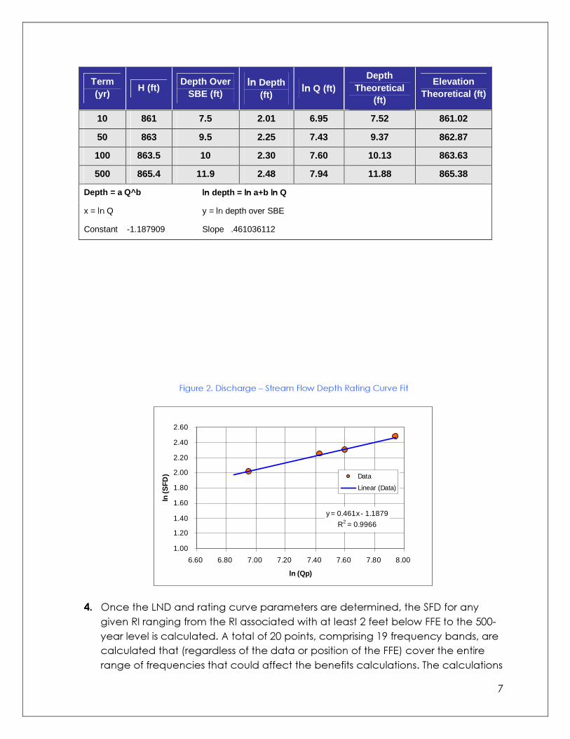
7

Term (yr)

H (ft) Depth Over

SBE (ft) ln Depth

(ft) ln Q (ft)

Depth Theoretical

(ft)

Elevation Theoretical (ft)

10 861 7.5 2.01 6.95 7.52 861.02

50 863 9.5 2.25 7.43 9.37 862.87

100 863.5 10 2.30 7.60 10.13 863.63

500 865.4 11.9 2.48 7.94 11.88 865.38

Depth = a Q^b ln depth = ln a+b ln Q

x = ln Q y = ln depth over SBE

Constant -1.187909 Slope .461036112

Figure 2. Discharge – Stream Flow Depth Rating Curve Fit

y = 0.461x - 1.1879

R2 = 0.9966

1.00

1.20

1.40

1.60

1.80

2.00

2.20

2.40

2.60

6.60 6.80 7.00 7.20 7.40 7.60 7.80 8.00

ln (Qp)

ln (S

FD) Data

Linear (Data)

4. Once the LND and rating curve parameters are determined, the SFD for any

given RI ranging from the RI associated with at least 2 feet below FFE to the 500-year level is calculated. A total of 20 points, comprising 19 frequency bands, are calculated that (regardless of the data or position of the FFE) cover the entire range of frequencies that could affect the benefits calculations. The calculations

8

of this stage are performed for three separate groups of points, each of which is handled in a different way:

a. For a user-input set of RIs (usually the Standard FIS RIs: 10-, 50-, 100-, and 500-year): i. For each given Qp, find the theoretical RI from the fitted LND. ii. For each given Qp, find the theoretical SFD from the rating curve. iii. Use the calculated SFD and add the SBE to get each WSE.

In this stage, the Qp and RI values for the data points are replaced by theoretical values that may be slightly different. This replacement helps to ensure a consistent set of results and a smooth EANF vs. FD curve.

b. For additional RIs (1.111, 2-, 5-, 8- 20-, 30-, 40-, 60-, 70-, 80-, 90-, 200-, 300-, and 400-year): i. For each RI, calculate P = 1 – (1/RI). (Where P = Probability) ii. For each P, find theoretical Qp from the inverse of the fitted LND. iii. Use the calculated Qp to find the SFD from the rating curve. iv. Use the calculated SFD and add the SBE to get each WSE.

c. For FD = minus 2 feet and 0 feet (WSE at FFE):

i. From WSE and FFE, determine the SFD of each point. ii. Using the SFD, find the theoretical Qp from the inverse of the rating

curve. iii. For each calculated Qp, find the RI from the fitted LND. iv. For each RI, calculate P = 1 – (1/RI).

Table 4. Calculations of Frequency Points

RI Data Discharge Theoretical

(cfs) P

RI Theoretical

(yr)

Elevation Theoretical

(ft)

Depth Over SBE

Theoretical/Data

Rank of RI

1.435 343.43 0.303 1.435 858.000 4.500 FFE – 2

ft 19

4.545 762.50 0.780 4.545 860.000 6.500 FFE 17

1.111 213.57 0.100 1.111 857.115 3.615 20

2.000 472.54 0.500 2.000 858.713 5.213 18

5.000 796.07 0.800 5.000 860.130 6.630 16

8.000 963.91 0.875 8.000 860.742 7.242 15

10 1045.90 0.900 10.009 861.020 7.520 14

9

20 1309.56 0.950 20.000 861.841 8.341 13

30 1472.34 0.967 30.000 862.304 8.804 12

40 1591.95 0.975 40.000 862.626 9.126 11

50 1685.50 0.980 49.801 862.870 9.370 10

60 1766.72 0.983 60.000 863.075 9.575 9

70 1835.12 0.986 70.000 863.245 9.745 8

80 1895.29 0.988 80.000 863.391 9.891 7

90 1949.06 0.989 90.000 863.519 10.019 6

100 1996.90 0.990 99.822 863.632 10.132 5

200 2331.74 0.995 200.000 864.382 10.882 4

300 2538.70 0.997 300.000 864.817 11.317 3

400 2690.95 0.998 400.000 865.125 11.625 2

500 2819.10 0.998 506.290 865.377 11.877 1

As seen in the table above, the RI calculated for the FFE is approximately 4.5 years and the RI calculated for FFE – 2 feet is 1.435 years. This means that having its FFE 1 foot below the 10-year flood stage results in this structure facing flooding (on the average) every 1.5 years. The following figures illustrate the extrapolation of the Qp-RI relationship and extrapolation of the rating curve, based on the results.

Figure 3. Extrapolation of Qp-RI Relationship

0

500

1000

1500

2000

2500

3000

0.1 1 10 100 1000

RI (Years)

Q (

cfs)

Q dataLog-NormalExtrapolateFFEFFE-2

10

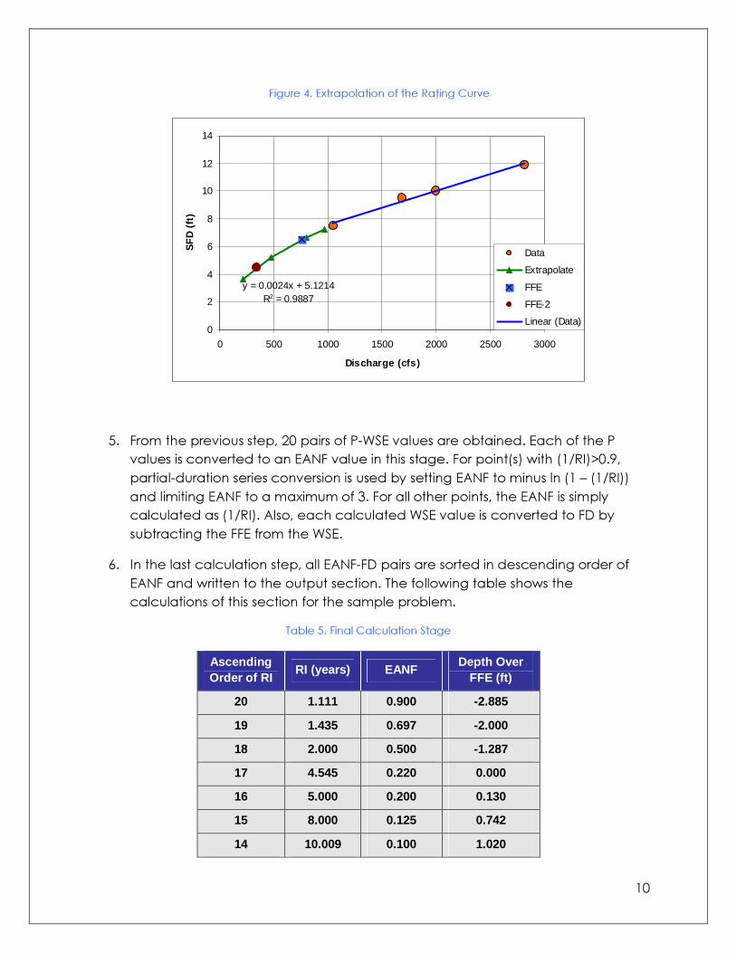
Figure 4. Extrapolation of the Rating Curve

y = 0.0024x + 5.1214R2 = 0.9887

0

2

4

6

8

10

12

14

0 500 1000 1500 2000 2500 3000

Discharge (cfs)

SF

D (

ft)

Data

Extrapolate

FFE

FFE-2

Linear (Data)

5. From the previous step, 20 pairs of P-WSE values are obtained. Each of the P

values is converted to an EANF value in this stage. For point(s) with (1/RI)>0.9, partial-duration series conversion is used by setting EANF to minus ln (1 – (1/RI)) and limiting EANF to a maximum of 3. For all other points, the EANF is simply calculated as (1/RI). Also, each calculated WSE value is converted to FD by subtracting the FFE from the WSE.

6. In the last calculation step, all EANF-FD pairs are sorted in descending order of EANF and written to the output section. The following table shows the calculations of this section for the sample problem.

Table 5. Final Calculation Stage

Ascending Order of RI

RI (years) EANF Depth Over

FFE (ft)

20 1.111 0.900 -2.885

19 1.435 0.697 -2.000

18 2.000 0.500 -1.287

17 4.545 0.220 0.000

16 5.000 0.200 0.130

15 8.000 0.125 0.742

14 10.009 0.100 1.020

11

13 20.000 0.050 1.841

12 30.000 0.033 2.304

11 40.000 0.025 2.626

10 49.801 0.020 2.870

9 60.000 0.017 3.075

8 70.000 0.014 3.245

7 80.000 0.013 3.391

6 90.000 0.011 3.519

5 99.822 0.010 3.632

4 200.000 0.005 4.382

3 300.000 0.003 4.817

2 400.000 0.003 5.125

1 506.290 0.002 5.377

12

The following table summarizes the results for the sample problem; the calculations are capable of providing an estimate of the results in the original Flood Full Data Module format of 1-foot elevation bands.

Table 6. Output Table

Results – Frequency Band 1-ft Elevation Band

Expected Annual Number of Floods Expected Annual Number

Flood Depth (ft) EANF Flood Depth (ft) EANF

-2.89 0.90000 -2 6.94E-01 -2.00 0.69672 -1 4.23E-01 -1.29 0.50000 0 2.19E-01 0.00 0.22003 1 1.01E-01 0.13 0.20000 2 4.34E-02 0.74 0.12500 3 1.78E-02 1.02 0.09991 4 7.15E-03 1.84 0.05000 5 2.83E-03 2.30 0.03333 6 1.12E-03 2.63 0.02500 7 4.40E-04 2.87 0.02008 8 1.75E-04 3.08 0.01667 >8 1.18E-04 3.24 0.01429 3.39 0.01250 3.52 0.01111 3.63 0.01002 4.38 0.00500 4.82 0.00333 5.13 0.00250 5.38 0.00198

The maximum FD calculated for this structure in the 20 frequency point method is 5.38 feet. This depth is below the maximum depth for this structure in the depth-damage tables. However, the RI of 5.38 feet of flooding for this structure is (approximately) 500 years, and any flooding above that level will have negligible effect on benefits calculations, due to a very small EANF. In this example, there are six EANF points calculated for FDs below the 10-year flood that gives an FD that equals 1 foot.

13

The following figure shows the EANF versus FD curve for the sample calculations. Figure 5. EANF vs. Flooding Depth Curve

EXPECTED ANNUAL NUMBER OF FLOODS vs FLOOD DEPTH

0.00

0.10

0.20

0.30

0.40

0.50

0.60

0.70

0.80

0.90

1.00

-4 -2 0 2 4 6 8 10

Flood Depth (ft)

EA

NF

1-ft Band Freq. Band

14

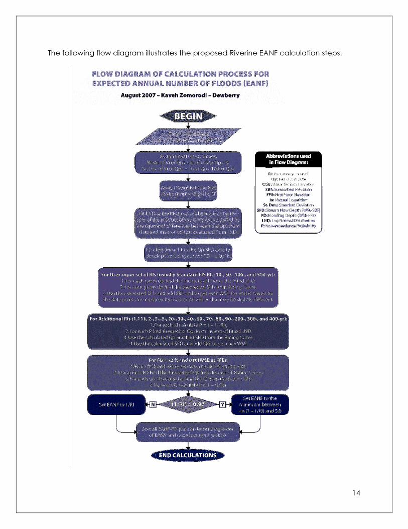
The following flow diagram illustrates the proposed Riverine EANF calculation steps.

15

For coastal flooding, the EANFs are determined by using the stillwater elevations provided by the analyst; the module requires the analyst to provide elevations for the 1- and 100-year events along with three other return periods. A linear relationship is established between x and y, as defined below:

1ElElElevationAdjustedtheisx RP −=

Where: El1 is the 1-year flood elevation. ElRP is the stillwater elevation for a given return period.

and

−=

−=

=

1

1ln

11

1

lnlnRP

RP

RPCDF

ExcPy

Where: ExcP is the probability of exceedance. CDF is the cumulative probability or probability of non-

exceedance of a flood depth with return period RP. RP is the return period.

The linear equation is:

)(1

1ln 1ElEliC

RPxiCy RP −+=

−→+=

Where: C is the constant found by linear intercept. i is the slope of the line.

Taking the exponential of both sides of the linear equation:

))((1

11ElEliCExp

RP RP −+=

−

16

Let the right-hand side of the equation be K:

K

K

KRP

KRPK

RP

+=+=→=−→=

−

11

111

1

1

This equation can be used to calculate the exceedance probability at various depths of flooding. For Z = minus 2.5 to 16.5 feet:

))((

11

11

1

11)(

1ElZiCExpKRP

ZExcP

−++=

+==

Where: Z is the Depth of Flooding in half-foot increments.

The EANF can be calculated by subtracting the exceedance probabilities of two consequent flood elevations. To ensure reasonability, the calculation is conditional for flooding depths that are close to the 1-year elevation. If the two consequently calculated values of flood elevation are both greater than the 1-year elevation, then their corresponding exceedance probabilities are simply subtracted from each other to find the EANF of that elevation band. If the higher elevation is higher than the 1-year flood, but the lower elevation is lower than the 1-year flood, then the EANF of that elevation band is set equal to one minus the exceedance probability of the higher elevation. If the higher elevation of an elevation band is equal to or smaller than the 1-year elevation, then the EANF of that elevation band is set to one.

1)()5.0(

)5.0(1)()5.0()5.0(

)5.0()5.0()()5.0()5.0(

1

11

11

=→≤+++−=→≤+−>++

+−+=→>+−>++

dEANFElFFEdIf

dExcPdEANFElFFEdANDElFFEdIf

dExcPdExcPdEANFElFFEdANDElFFEdIf

Where: EANF(d) is the Expected Annual Number of Floods at depth d.

d is the Depth of Flooding (which typically ranges from minus 2 feet to 16 feet, but the actual range depends on the DDF associated with the building type).

FFE is the First Floor Elevation of the building.

17

The following figure illustrates the results of the coastal EANF calculations. Table 7. Coastal Frequency Rates Figure 6. Coastal EANF Graph

Depth

feet

Expected Annual

Number of Floods

-8 1

Elevation 3 -7 1 Frequency A 10 -6 1 Frequency B 50 -5 1

Frequency C 100 -4 1 Frequency D 500 -3 1 Base Flood Elevation (BFE) 10.8 -2 1

1 Year 2.5 -1 1 10 Year 4.2 0 0.895001016 50 Year 8.9 1 0.025566275 100 Year 10.8 2 0.019756203 500 Year 17.2 3 0.015080554

4 0.011404141 1 Year 2.5 5 0.008563035 10 Year 4.2 6 0.006395551 50 Year 8.9 7 0.004757712 100 Year 10.8 8 0.00352883 500 Year 17.2 >8 0.009946683

Flood Discharge Data

Description: Flow rates for various flood events. Problem: Methodology Update List Item Number FD–011 requires that the BCAR effort ensure that the re-engineered Flood Full Data Module has the flexibility for different before- and after-mitigation flood hazard conditions. Recommendation: Integrate the flexibility to have different before- and after-mitigation discharge values. Changes: The user will be able to enter before- and after-mitigation discharge values, if they differ.

18

Flood Elevation Data

Description: Specific values read from flood profiles (contained in the FIS) for the project location; for the Coastal Zone A and V modules, the 1-year flood elevation data is required. Problem: Methodology Update List Item Numbers VZ–001 and VZ–003 require that the BCAR effort incorporate a wave-height factor with any coastal flood BCA and evaluate the need for retaining the 1-year coastal flood evaluation. In addition, Item Number FD–011 requires that the BCAR effort ensure that the re-engineered Flood Full Data Module has the flexibility to accommodate different before- and after-mitigation flood hazard conditions. Recommendation: Elevations for the 10-, 50-, 100-, and 500-year flood provided by a flood profile or summary of the Stillwater Elevations Table (contained in the FIS) will be required. To ensure that an EANF greater than one does not occur, the 1-year flood elevation will continue to be required for projects subject to coastal flooding. Changes: The user will be able to enter before- and after-mitigation elevation values, if they differ. A wave-height factor will be applied to all coastal scenarios regardless of whether they are located in the Coastal Zone A or Coastal Zone V. To apply the wave-height factor, the analyst will have to provide the Base Flood Elevation (BFE) along with the stillwater elevations. The ratio between the BFE and the 100-year stillwater elevation will be applied to all of the stillwater elevations, as follows:

=

100_ )(

El

BFEElEl RPAdjustedRP

Where: El100 is the 100-year flood elevation or the BFE. ElRP is the stillwater elevation for a given return period. BFE is the Base Flood Elevation.

19

For riverine scenarios, the user will be required to provide standard elevation points, as well as values representing the SBE. For coastal scenarios, a table of 1-year elevations and/or a link to the National Oceanic and Atmospheric Administration (NOAA) Tides and Currents Web site will be provided. Links to the FEMA Map Service Center Web site will be provided as well.

Excepted Damages The expected losses at specific flood depths are determined by using the value of the property exposed and the DDFs built into the module.

))(()( VDDFdL =

Where: L(d) is the expected losses or damages at depth d. DDF is the Depth Damage Function, expressed in percentage or

days, depending upon the category. V is the value of property exposed, expressed in dollars.

In the Flood Full Data Module, damages are categorized as follows: � Building � Contents � Displacement � Lost Business Income � Loss of Rental Income � Value of Lost Public/Nonprofit Service � Other

Building Damages Building damages are estimated as the product of the Building DDF and the Building Replacement Value (BRV).

20

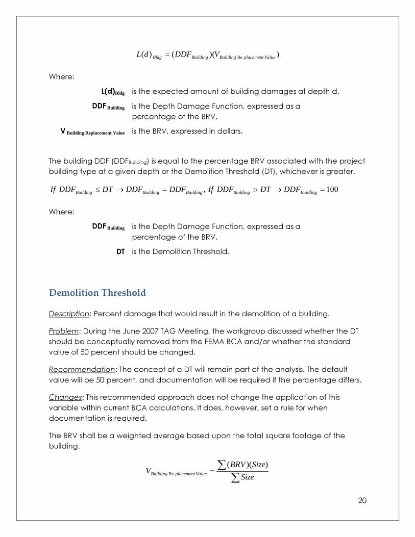
))(()( Re ValueplacementBuildingBuildingBldg VDDFdL =

Where: L(d)Bldg is the expected amount of building damages at depth d.

DDF Building is the Depth Damage Function, expressed as a percentage of the BRV.

V Building Replacement Value is the BRV, expressed in dollars. The building DDF (DDFBuilding) is equal to the percentage BRV associated with the project building type at a given depth or the Demolition Threshold (DT), whichever is greater.

100, =→>=→≤ BuildingBuildingBuildingBuildingBuilding DDFDTDDFIfDDFDDFDTDDFIf

Where: DDF Building is the Depth Damage Function, expressed as a

percentage of the BRV. DT is the Demolition Threshold.

Demolition Threshold Description: Percent damage that would result in the demolition of a building. Problem: During the June 2007 TAG Meeting, the workgroup discussed whether the DT should be conceptually removed from the FEMA BCA and/or whether the standard value of 50 percent should be changed. Recommendation: The concept of a DT will remain part of the analysis. The default value will be 50 percent, and documentation will be required if the percentage differs. Changes: This recommended approach does not change the application of this variable within current BCA calculations. It does, however, set a rule for when documentation is required. The BRV shall be a weighted average based upon the total square footage of the building.

∑∑=

Size

SizeBRVV ValueplacementBuilding

))((Re

21

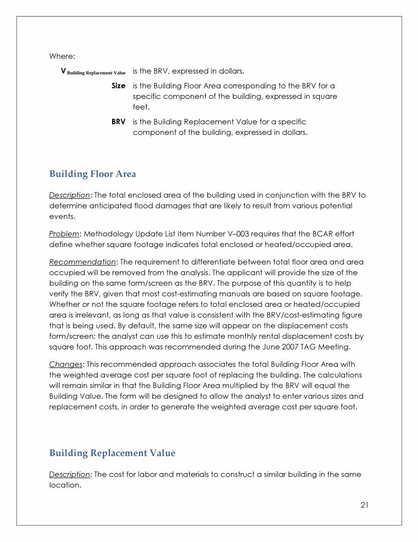
Where: V Building Replacement Value is the BRV, expressed in dollars.

Size is the Building Floor Area corresponding to the BRV for a specific component of the building, expressed in square feet.

BRV is the Building Replacement Value for a specific component of the building, expressed in dollars.

Building Floor Area Description: The total enclosed area of the building used in conjunction with the BRV to determine anticipated flood damages that are likely to result from various potential events. Problem: Methodology Update List Item Number V–003 requires that the BCAR effort define whether square footage indicates total enclosed or heated/occupied area. Recommendation: The requirement to differentiate between total floor area and area occupied will be removed from the analysis. The applicant will provide the size of the building on the same form/screen as the BRV. The purpose of this quantity is to help verify the BRV, given that most cost-estimating manuals are based on square footage. Whether or not the square footage refers to total enclosed area or heated/occupied area is irrelevant, as long as that value is consistent with the BRV/cost-estimating figure that is being used. By default, the same size will appear on the displacement costs form/screen; the analyst can use this to estimate monthly rental displacement costs by square foot. This approach was recommended during the June 2007 TAG Meeting. Changes: This recommended approach associates the total Building Floor Area with the weighted average cost per square foot of replacing the building. The calculations will remain similar in that the Building Floor Area multiplied by the BRV will equal the Building Value. The form will be designed to allow the analyst to enter various sizes and replacement costs, in order to generate the weighted average cost per square foot.

Building Replacement Value Description: The cost for labor and materials to construct a similar building in the same location.

22

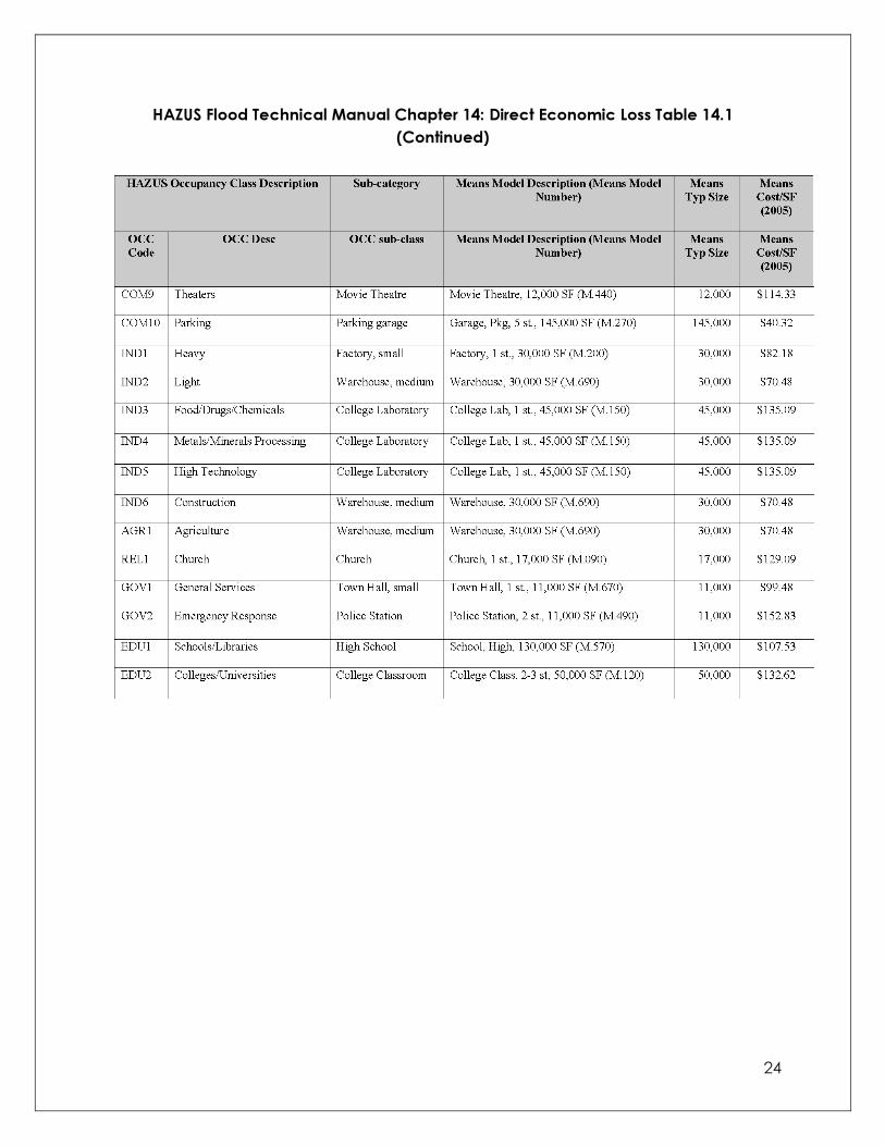
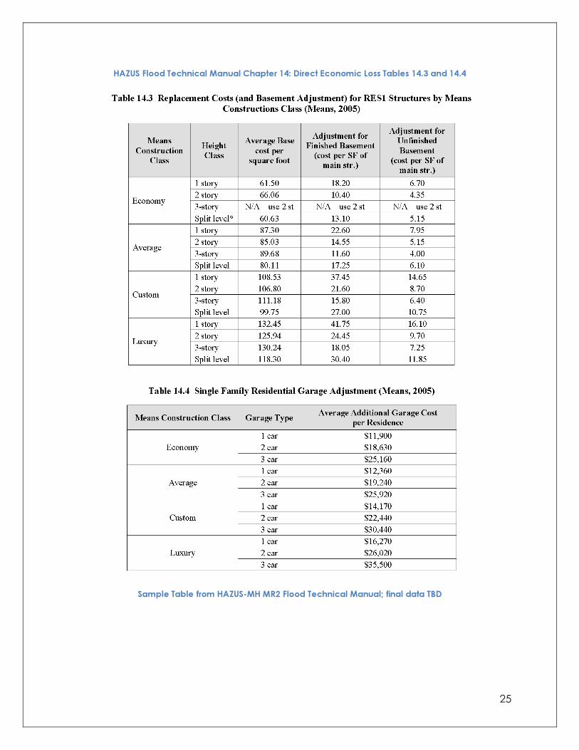
Problem: Methodology Update List Item Number S–008 requires that the BCAR effort allow the user to differentiate between total and unit cost, and incorporate a toggle switch so that an analyst can enter the value in either format. Recommendation: The BRV will remain part of the module. However, the form/screen will only require that the analyst provide a size for the value that he or she is using. For example, the user may have a cost estimate for three separate areas (e.g., the heated area, garage, and a patio) and separate sizes and values can be entered for each of these areas. The BRV shall be a weighted average based upon the total square footage of the building. If the size is unknown, the analyst may provide a lump-sum cost for the building, but this will be an alternate option—not the default. A table will be provided with BRVs for analysts to use as a rule of thumb (see the Hazards U.S. [HAZUS] Direct Economic Loss Tables 14.1, 14.3, and 14.4). Documentation will be required to justify values selected from the tables or any other source, as there is no default value for BRV. Changes: The calculations will remain the same, in that the Building Floor Area multiplied by the BRV will generate the Building Value, unless a lump-sum cost is provided.

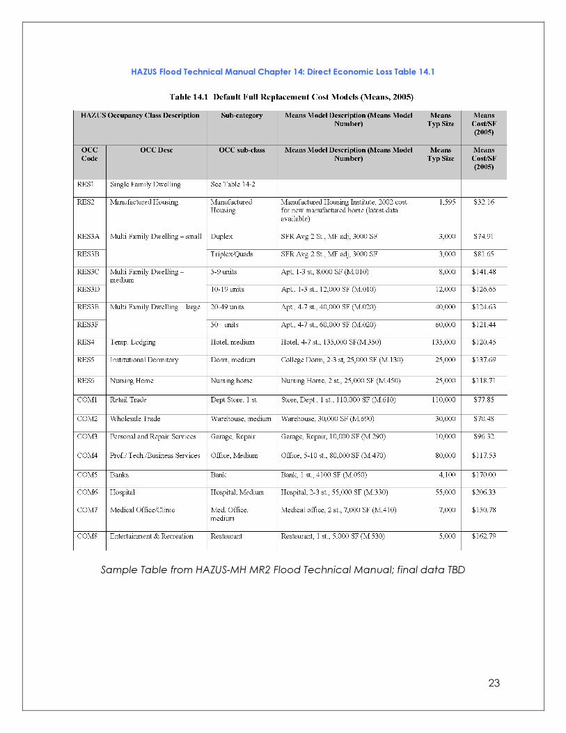
23

HAZUS Flood Technical Manual Chapter 14: Direct Economic Loss Table 14.1

Sample Table from HAZUS-MH MR2 Flood Technical Manual; final data TBD

24

HAZUS Flood Technical Manual Chapter 14: Direct Economic Loss Table 14.1 (Continued)

25

HAZUS Flood Technical Manual Chapter 14: Direct Economic Loss Tables 14.3 and 14.4


26

Content Damages Content damages are estimated as the product of the Content DDF and the Value of Contents.

))(()( ValueContentContentCont VDDFdL =

Where: L(d)Cont is the expected amount of content damages at depth d.

DDF Content is the Depth Damage Function, expressed as a percentage of the Value of Contents.

V Content Value is the Value of Contents exposed to flooding, expressed in dollars.

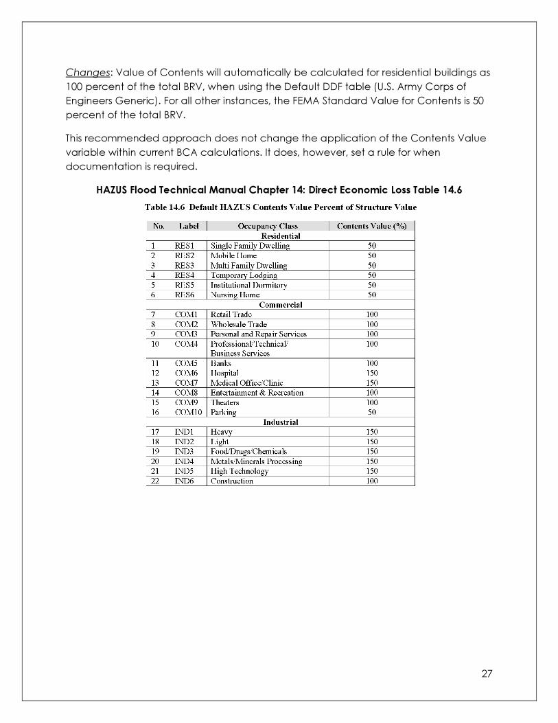
Value of Contents Description: The cost to replace the contents of a building. Problem: Methodology Update List Item Number V–004 requires that the BCAR effort revise the default value for residential contents. During the June 2007 TAG Meeting, the workgroup discussed using 50 percent of the BRV as the default for residential buildings and also discussed ensuring that the software provide rules of thumb for other building types (such as the table in FEMA 386–2, the source of which is HAZUS). Recommendation: By default, the Value of Contents will automatically be calculated for residential buildings as 100 percent of the total BRV (or whatever the final value/guidance is in the FEMA publication What Is a Benefit? or WIAB), when using the Default DDF table (U.S. Army Corps of Engineers Generic). For all other instances, the default Contents Value is 50 percent of the total BRV. The analyst can override this value, but documentation will then be required. A table will be provided for commercial buildings for analysts to use as a rule of thumb. Sources for this table will be HAZUS, FEMA Mitigation Planning How-To Guide #2, Understanding Your Risks: Identifying Hazards and Estimating Losses FEMA 386–2, and the USACE (see HAZUS Direct Economic Loss Tables 14.6 for sample values). Documentation will always be required for commercial buildings and for residential buildings when the value is greater than 50 percent of the total BRV.

27

Changes: Value of Contents will automatically be calculated for residential buildings as 100 percent of the total BRV, when using the Default DDF table (U.S. Army Corps of Engineers Generic). For all other instances, the FEMA Standard Value for Contents is 50 percent of the total BRV. This recommended approach does not change the application of the Contents Value variable within current BCA calculations. It does, however, set a rule for when documentation is required.


28

Sample Table from HAZUS-MH MR2 Flood Technical Manual

Displacement Costs Displacement Costs are those borne by occupants during the time when a building becomes uninhabitable due to flood damage. These costs are estimated as the product of the displacement days based on the DDF and the Displacement Costs per day.

))(()( CostntDisplacementDisplacemeDisp VDDFdL =

Where: L(d)Disp is the expected amount of Displacement Costs at depth

d. DDF Displacement is the Displacement Depth Damage Function, expressed

in days. V Displacement Cost is the daily Displacement Costs, expressed in dollars.

Problem: Methodology Update List Item Number V–008 requires that the BCAR effort increase the standard displacement time and costs; this problem is more related to guidance and values than methodology or calculations. During the June 2007 TAG Meeting, the workgroup discussed integrating “Disruption of Life” into displacement benefits. Recommendation: Displacement Costs will continue to be broken down into three parts: • Monthly cost of temporary living space • Other monthly costs related to displacement

29

• One-time Displacement Costs The cost of temporary living space may be based upon a cost per square foot or a lump sum. For example, the user may base the analysis on the cost of two hotel rooms or a three-bedroom apartment in the area, versus 2,000 square feet of living space. Default values will be provided and documentation will be required if these are overwritten. A table will be provided with Displacement Costs for analysts to use as a rule of thumb (see HAZUS Direct Economic Loss Tables 14.10). Documentation will be required to justify values selected from the tables (or any other source), as there is no default value given for Displacement Costs. Changes: This recommended approach does not change the application of this variable within current BCA calculations. It does, however, set a rule governing when documentation is required.

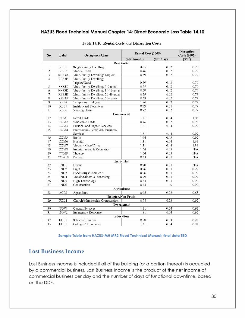
30



Lost Business Income Lost Business Income is included if all of the building (or a portion thereof) is occupied by a commercial business. Lost Business Income is the product of the net income of commercial business per day and the number of days of functional downtime, based on the DDF.

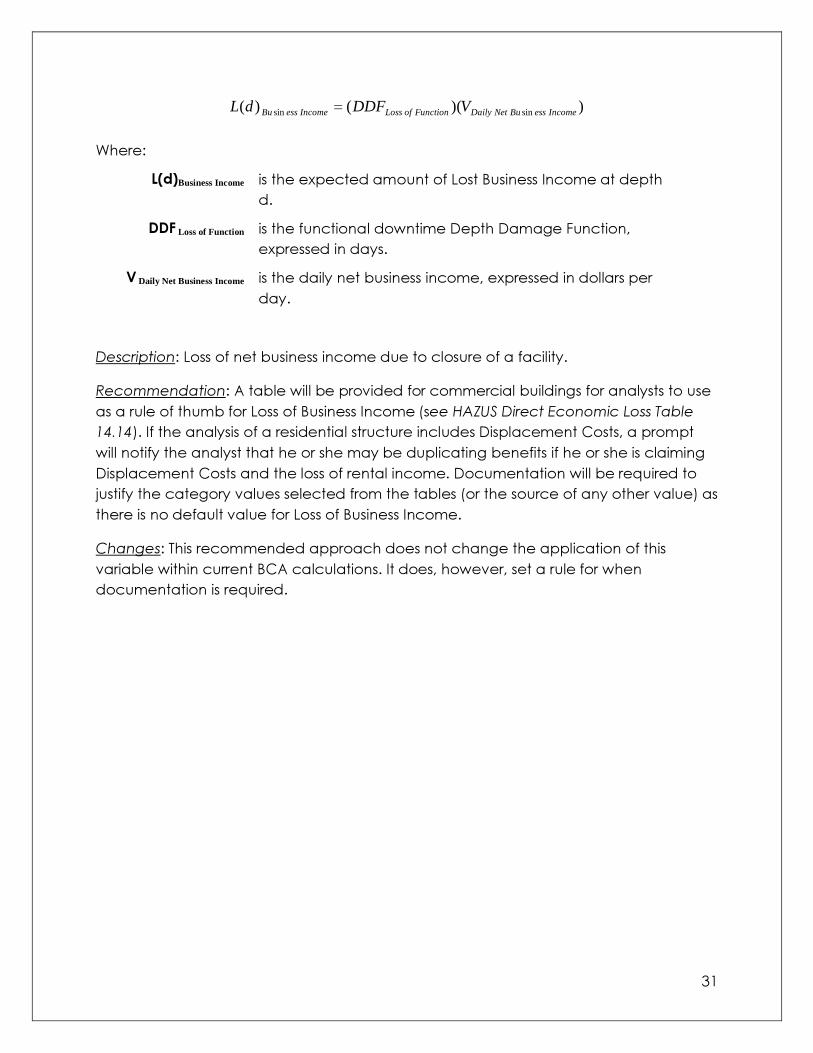
31

))(()( sinsin IncomeessBuNetDailyFunctionofLossIncomeessBu VDDFdL =

Where: L(d)Business Income is the expected amount of Lost Business Income at depth

d. DDF Loss of Function is the functional downtime Depth Damage Function,

expressed in days. V Daily Net Business Income is the daily net business income, expressed in dollars per

day. Description: Loss of net business income due to closure of a facility. Recommendation: A table will be provided for commercial buildings for analysts to use as a rule of thumb for Loss of Business Income (see HAZUS Direct Economic Loss Table 14.14). If the analysis of a residential structure includes Displacement Costs, a prompt will notify the analyst that he or she may be duplicating benefits if he or she is claiming Displacement Costs and the loss of rental income. Documentation will be required to justify the category values selected from the tables (or the source of any other value) as there is no default value for Loss of Business Income. Changes: This recommended approach does not change the application of this variable within current BCA calculations. It does, however, set a rule for when documentation is required.

32



33

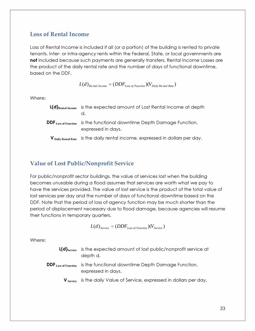
Loss of Rental Income Loss of Rental Income is included if all (or a portion) of the building is rented to private tenants. Inter- or intra-agency rents within the Federal, State, or local governments are not included because such payments are generally transfers. Rental Income Losses are the product of the daily rental rate and the number of days of functional downtime, based on the DDF.

))(()( ReRe RatentalDailyFunctionofLossIncomental VDDFdL =

Where: L(d)Rental Income is the expected amount of Lost Rental Income at depth

d. DDF Loss of Function is the functional downtime Depth Damage Function,

expressed in days. V Daily Rental Rate is the daily rental income, expressed in dollars per day.

Value of Lost Public/Nonprofit Service For public/nonprofit sector buildings, the value of services lost when the building becomes unusable during a flood assumes that services are worth what we pay to have the services provided. The value of lost service is the product of the total value of lost services per day and the number of days of functional downtime based on the DDF. Note that the period of loss of agency function may be much shorter than the period of displacement necessary due to flood damage, because agencies will resume their functions in temporary quarters.

))(()( ServiceFunctionofLossService VDDFdL =

Where: L(d)Service is the expected amount of lost public/nonprofit service at

depth d. DDF Loss of Function is the functional downtime Depth Damage Function,

expressed in days. V Service is the daily Value of Service, expressed in dollars per day.

34

Value of Service

For information on the Value of Public Services please see the FEMA BCAR Risk Analysis Methodology Report.

Crawlspace Description: To account for damages to crawlspace contents the software assumes the crawlspace (when applicable/entered) are damaged starting at a flood depth of -1 foot and continues throughout all flood depths.

Other The module allows the analyst to include other benefits that have not been covered by the basic Full Data Module, but are allowed based on WIAB. The analyst will have to associate quantified damages with a frequency or depth of flooding. For example, the analyst may have statistics to show that homeowners will save $1,000 a year in flood insurance premiums. This interface will allow the user to relate an infinite amount of benefits data with his/her analysis/structure, as long as the benefit is in an accepted category in WIAB and can be annualized or associated with a depth of flooding. Part of the form for this interface will include a pull-down menu of “other” benefit categories.

OtherOther RPLordL )()(

Where: L(d)Other is the expected amount of other damages avoided at

depth d. L(RP)Other is the expected amount of other damages avoided for

return period RP. Total Expected Damages The total expected damages are the sum of the damage categories.

+++++++=

])()([)()(

)()()()()(

ServiceIncome Rental

Income Business

OtherOther

DispContBldg

TotalRPLordLdLdL

dLdLdLdLdL

35

Depth Damage Functions DDFs are used to estimate expected flood damages for various types of buildings, their contents, or their functions at different water depths. This relationship is expressed as depth versus percentage of damage to the element being considered. The depths for the DDFs integrated into the module typically range from minus 2 to 16 feet. The Flood Full Data Module calculates damages at flood depths based on the DDF associated with the building type selected by the analyst.

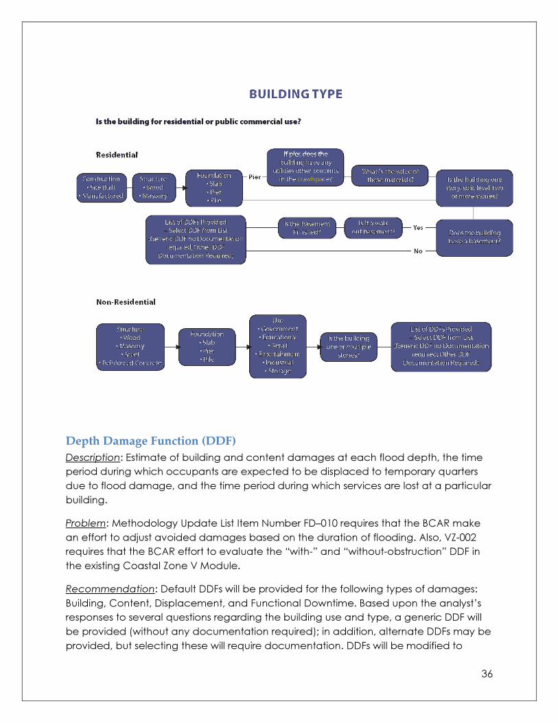
Building Type Description: The building type determines which built-in DDFs to use. Problem: The building types need to be clearly defined for the users as part of the module. Recommendation: Defining the building type will remain a part of the module, but the manner of its selection will differ greatly. The current module has a list of six building types for the analyst to choose from; the new software will incorporate a group of questions that helps guide the analyst to a specific building type. Changes: This recommended approach does not change the application of this variable within current BCA calculations; it modifies the process of selecting the DDFs that best represent the building associated with the particular mitigation project being analyzed. The following diagram contrasts residential and non-residential construction methods as they relate to different types of buildings.

36

Depth Damage Function (DDF) Description: Estimate of building and content damages at each flood depth, the time period during which occupants are expected to be displaced to temporary quarters due to flood damage, and the time period during which services are lost at a particular building. Problem: Methodology Update List Item Number FD–010 requires that the BCAR make an effort to adjust avoided damages based on the duration of flooding. Also, VZ-002 requires that the BCAR effort to evaluate the “with-” and “without-obstruction” DDF in the existing Coastal Zone V Module. Recommendation: Default DDFs will be provided for the following types of damages: Building, Content, Displacement, and Functional Downtime. Based upon the analyst’s responses to several questions regarding the building use and type, a generic DDF will be provided (without any documentation required); in addition, alternate DDFs may be provided, but selecting these will require documentation. DDFs will be modified to

37

provide a standard approach for walkout basements, crawl spaces, or Coastal Zone V conditions. In addition, DDFs for long-duration flooding events will be provided. Changes: This recommended approach does not change the application of this variable within current BCA calculations. It does, however, provide a much greater number of DDFs for the analyst to choose from.

Benefits The expected annual net benefits (EAB) are the difference between expected annual damages before (EADBefore Mitigation) and after (EADAfter Mitigation) mitigation.

MitigationAfterMitigationBefore EADEADEAB −=

Where: EAB is the expected annual net benefit.

EADBefore Mitigation is the expected annual damages before mitigation. EADAfter Mitigation is the expected annual damages after mitigation.

The depth of flooding for Before-Mitigation Damages are calculated based on the First Floor Elevation (FFE).

∑=

−=

==

16

2

)]()][([)(d

dMitigationBefore dLdEANFdEADEAD

Where: d is 0 at the FFE.

EAD(d) is the expected annual damage at depth d. EANF(d) is the Expected Annual Number of Floods at depth d.


First Floor Elevation (FFE) Description: The FFE is the elevation at the top of the finished flooring of a structure’s lowest floor. Problem: Methodology Update List Item Number G–017 requires that the BCAR effort provide guidance on the FFE for buildings with walkout basements.

38

Recommendation: Specific guidance will be provided on the FFE regarding walkout basements and other common issues (e.g., crawl spaces). The FFE will be input after the building type is defined so the guidance will be specific to that scenario. In addition, the analyst must provide documentation; the source of the FFE should have 0.5-foot of accuracy. Finally the FFE will be defined based upon the building type (e.g., first floor, lowest horizontal member, basement, etc.). Changes: This recommended approach does not change the application of this variable within current BCA calculations. The depth of flooding for After-Mitigation Damages are calculated based on the FFE plus the height the building is being elevated. There are no After-Mitigation Damages for acquisition projects. An acquisition project is the only type of mitigation project that completely eliminates future damages and losses.

∑=

−=

==

16

2

)]()][([)(d

dMitigationAfter dLdEANFdEADEAD

Where: d is 0 at the FFE plus the amount that the building is being

elevated. EAD(d) is the expected annual damage at depth d. EANF(d) is the Expected Annual Number of Floods at depth d.


∑−=

=

16

2d

EABB

Where: B is the total expected annual benefit of the hazard mitigation

project. d is the depth of flooding.

EAB is the expected annual net benefit.

MitigationAfter

T

MitigationBefore

T

oject r

rB

r

rBB

+−−

+−=−− )1(1)1(1

Pr

39

Where: BProject is the total benefit of the hazard mitigation project.

B is the total expected annual benefit of the hazard mitigation project.

T is the estimated amount of time (in years) that the mitigation action will be effective (also called the Project Useful Life).

R is the annual Discount Rate used to determine the Net Present Value of benefits. For FEMA-funded projects, the rate is set by the OMB.

Mitigation Project Useful Lifetime

Description: Estimated amount of time (in years) that a mitigation project will remain effective. Problem: The methodology must outline the most effective determine the Mitigation Project Useful Lifetime. Recommendation: Values from the Project Useful Life Summary Table will be provided based upon responses to certain questions. For example: � Acquisition = 100 years � Elevation = 30 years � Major Infrastructure = 50 years

Documentation will be required if the recommended values are overwritten. Changes: This recommended approach does not change the application of this variable within current BCA calculations. It does, however, set a rule governing when documentation is required.

Discount Rate Description: The discount rate determines the time-value of money and is mandated by the OMB to be 7 percent for all BCAs. Problem: Methodology Update List Item Number V–001 requires that the BCAR effort coordinate with OMB to lower the current value. FEMA will be taking the lead in contacting OMB for discussions about the discount rate. The team will provide assistance, as requested by FEMA.

40

Recommendation: The discount rate will remain part of the module. However, the analyst must provide documentation if he/she changes the default value (documentation automatically becomes a required field on change to the discount rate). If OMB changes the discount rate, the default value will be modified in the next release of BCA software updates. Changes: This recommended approach does not change the application of this variable within current BCA calculations. The BCR is the benefits of the mitigation project (BProject) divided by the costs (CProject) of the mitigation project.

oject

oject

C

BBCR

Pr

Pr=

Where: BCR is the Benefit-Cost Ratio.

BProject is the total benefit of the hazard mitigation project. CProject is the total net present value of the cost of the hazard mitigation

project.

fema benefit-cost analysis re-engineering (bcar) · fema benefit-cost analysis re-engineering...

Documents