felt manual
TRANSCRIPT

7/30/2019 Felt Manual
http://slidepdf.com/reader/full/felt-manual 1/236

7/30/2019 Felt Manual
http://slidepdf.com/reader/full/felt-manual 2/236

7/30/2019 Felt Manual
http://slidepdf.com/reader/full/felt-manual 3/236
FElt: User’s Guide and Reference Manual
Jason I. Gobat Applied Physics Laboratory
University of Washington
Darren C. Atkinson Department of Computer Engineering
Santa Clara University
Computer Science Technical Report CS94-376University of California, San Diego

7/30/2019 Felt Manual
http://slidepdf.com/reader/full/felt-manual 4/236
Legal NoticeCopyright c 1993 – 2005 Jason Gobat and Darren Atkinson
[email protected] and [email protected]
“The FElt System: User’s Guide and Reference Manual” may be reproduced and distributed inwhole or in part, subject to the following conditions:
0. The copyright notice above and this permission notice must be preserved complete on all
complete or partial copies.
1. Any translation or derivative work of “The FElt System: User’s Guide and Reference Man-
ual” must be approved by the authors in writing before distribution.
2. If you distribute “The FElt System: User’s Guide and Reference Manual” in part, instruc-
tions for obtaining the complete version of “The FElt System: User’s Guide and Reference
Manual” must be included, and a means for obtaining a complete version provided.
3. Small portions may be reproduced as illustrations for reviews or quotes in other works
without this permission notice if proper citation is given.
4. The GNU General Public License referenced below may be reproduced under the condi-
tions given within it.
All source code in the FElt system is placed under the GNU General Public License. See ap-
pendix B for a copy of the GNU “GPL.”
The authors are not liable for any damages, direct or indirect, resulting from the use of information
provided in this document.
7/30/2019 Felt Manual
http://slidepdf.com/reader/full/felt-manual 5/236
Contents
Foreword xvii
About this Manual . . . . . . . . . . . . . . . . . . . . . . . . . . . . . . . . . xvii
Organization of this Manual . . . . . . . . . . . . . . . . . . . . . . . . . . . . xvii
Typographical Conventions . . . . . . . . . . . . . . . . . . . . . . . . . . . . . xviii
Acknowledgements . . . . . . . . . . . . . . . . . . . . . . . . . . . . . . . . . xix
1 Introduction to the FElt System 1
1.1 Intentions . . . . . . . . . . . . . . . . . . . . . . . . . . . . . . . . . . . 1
1.2 FElt: What it can do for you . . . . . . . . . . . . . . . . . . . . . . . . . 2
1.3 FElt: What it cannot do for you . . . . . . . . . . . . . . . . . . . . . . . . 3
2 FElt Analysis Types 5
2.1 Introduction . . . . . . . . . . . . . . . . . . . . . . . . . . . . . . . . . . 5
2.2 Static structural analysis . . . . . . . . . . . . . . . . . . . . . . . . . . . 5
2.3 Transient structural analysis . . . . . . . . . . . . . . . . . . . . . . . . . 7
2.4 Static thermal analysis . . . . . . . . . . . . . . . . . . . . . . . . . . . . 8
2.5 Transient thermal analysis . . . . . . . . . . . . . . . . . . . . . . . . . . 8
2.6 Modal analysis . . . . . . . . . . . . . . . . . . . . . . . . . . . . . . . . 8
2.7 Spectral analysis . . . . . . . . . . . . . . . . . . . . . . . . . . . . . . . 10
2.8 Nonlinear static analysis . . . . . . . . . . . . . . . . . . . . . . . . . . . 11
2.9 Nonlinear dynamic analysis . . . . . . . . . . . . . . . . . . . . . . . . . . 11
iii
7/30/2019 Felt Manual
http://slidepdf.com/reader/full/felt-manual 6/236
iv CONTENTS
3 Structure of a FElt Problem 13
3.1 Input file syntax . . . . . . . . . . . . . . . . . . . . . . . . . . . . . . . . 13
3.1.1 General rules . . . . . . . . . . . . . . . . . . . . . . . . . . . . . 13
3.1.2 Expressions . . . . . . . . . . . . . . . . . . . . . . . . . . . . . . 14
3.1.2.1 Continuous functions . . . . . . . . . . . . . . . . . . . 14
3.1.2.2 Discrete functions . . . . . . . . . . . . . . . . . . . . . 14
3.1.3 Units . . . . . . . . . . . . . . . . . . . . . . . . . . . . . . . . . 16
3.1.4 A simple example . . . . . . . . . . . . . . . . . . . . . . . . . . 16
3.2 Sections of a FElt input file . . . . . . . . . . . . . . . . . . . . . . . . . . 17
3.2.1 Problem description . . . . . . . . . . . . . . . . . . . . . . . . . 17
3.2.2 Nodes . . . . . . . . . . . . . . . . . . . . . . . . . . . . . . . . . 17
3.2.3 Elements . . . . . . . . . . . . . . . . . . . . . . . . . . . . . . . 18
3.2.4 Material properties . . . . . . . . . . . . . . . . . . . . . . . . . . 18
3.2.5 Constraints . . . . . . . . . . . . . . . . . . . . . . . . . . . . . . 19
3.2.6 Forces . . . . . . . . . . . . . . . . . . . . . . . . . . . . . . . . . 20
3.2.7 Distributed loads . . . . . . . . . . . . . . . . . . . . . . . . . . . 21
3.2.8 Analysis parameters . . . . . . . . . . . . . . . . . . . . . . . . . 22
3.2.9 Load cases . . . . . . . . . . . . . . . . . . . . . . . . . . . . . . 22
3.3 An illustrated example . . . . . . . . . . . . . . . . . . . . . . . . . . . . 22
3.4 An example of a transient analysis problem . . . . . . . . . . . . . . . . . 25
3.5 Format conversion . . . . . . . . . . . . . . . . . . . . . . . . . . . . . . 27
3.5.1 Conversion basics . . . . . . . . . . . . . . . . . . . . . . . . . . 27
3.5.2 patchwork details . . . . . . . . . . . . . . . . . . . . . . . . . . . 28
4 The FElt Element Library 29
4.1 Introduction . . . . . . . . . . . . . . . . . . . . . . . . . . . . . . . . . . 29
4.2 Structural analysis elements . . . . . . . . . . . . . . . . . . . . . . . . . 30
4.2.1 Truss and spring elements . . . . . . . . . . . . . . . . . . . . . . 30

7/30/2019 Felt Manual
http://slidepdf.com/reader/full/felt-manual 7/236
CONTENTS v
4.2.2 Euler-Bernoulli beam elements . . . . . . . . . . . . . . . . . . . . 31
4.2.2.1 Special case two-dimensional element . . . . . . . . . . 31
4.2.2.2 Arbitrarily oriented three-dimensional element . . . . . . 34
4.2.3 Timoshenko beam element . . . . . . . . . . . . . . . . . . . . . . 34
4.2.4 Constant Strain Triangular (CST) elements . . . . . . . . . . . . . 35
4.2.5 Two-dimensional isoparametric elements . . . . . . . . . . . . . . 36
4.2.5.1 General four to nine node element . . . . . . . . . . . . 36
4.2.5.2 Simple four node element . . . . . . . . . . . . . . . . . 37
4.2.6 Plate bending element . . . . . . . . . . . . . . . . . . . . . . . . 37
4.2.7 Solid brick element . . . . . . . . . . . . . . . . . . . . . . . . . . 39
4.2.8 Axisymmetric elements . . . . . . . . . . . . . . . . . . . . . . . 40
4.3 Thermal analysis elements . . . . . . . . . . . . . . . . . . . . . . . . . . 40
4.3.1 Rod element . . . . . . . . . . . . . . . . . . . . . . . . . . . . . 40
4.3.2 Constant Temperature Gradient (CTG) element . . . . . . . . . . . 40
5 The felt Application 41
5.1 Using felt . . . . . . . . . . . . . . . . . . . . . . . . . . . . . . . . . . . 41
5.2 Solving a problem . . . . . . . . . . . . . . . . . . . . . . . . . . . . . . . 44
5.3 Interpreting the output from felt . . . . . . . . . . . . . . . . . . . . . . . 44
5.3.1 Static analysis . . . . . . . . . . . . . . . . . . . . . . . . . . . . 44
5.3.2 Transient analysis . . . . . . . . . . . . . . . . . . . . . . . . . . . 47
5.3.3 Modal analysis . . . . . . . . . . . . . . . . . . . . . . . . . . . . 49
5.3.4 Thermal analysis . . . . . . . . . . . . . . . . . . . . . . . . . . . 51
5.3.5 Spectral analysis . . . . . . . . . . . . . . . . . . . . . . . . . . . 51
6 Using WinFElt 53
6.1 Introduction to WinFElt . . . . . . . . . . . . . . . . . . . . . . . . . . . . 53
6.2 Solving a problem . . . . . . . . . . . . . . . . . . . . . . . . . . . . . . . 53
6.3 Text output . . . . . . . . . . . . . . . . . . . . . . . . . . . . . . . . . . 56

7/30/2019 Felt Manual
http://slidepdf.com/reader/full/felt-manual 8/236

7/30/2019 Felt Manual
http://slidepdf.com/reader/full/felt-manual 9/236
CONTENTS vii
7.9.1 Generating a grid of line or quadrilateral elements . . . . . . . . . 81
7.9.2 Generating a mesh of triangular elements . . . . . . . . . . . . . . 81
7.10 Keyboard interface mechanisms . . . . . . . . . . . . . . . . . . . . . . . 82
7.10.1 Keyboard shortcuts . . . . . . . . . . . . . . . . . . . . . . . . . . 82
7.10.2 Command names . . . . . . . . . . . . . . . . . . . . . . . . . . . 83
7.11 Command line options . . . . . . . . . . . . . . . . . . . . . . . . . . . . 85
8 Post-processing with velvet 87
8.1 Solving a problem with velvet . . . . . . . . . . . . . . . . . . . . . . . . 87
8.2 Problem description and analysis parameters . . . . . . . . . . . . . . . . . 92
8.3 Controlling the post-processing . . . . . . . . . . . . . . . . . . . . . . . . 92
8.3.1 Controlling contour plots . . . . . . . . . . . . . . . . . . . . . . . 92
8.3.2 Controlling structure plots . . . . . . . . . . . . . . . . . . . . . . 94
8.3.3 Controlling animation . . . . . . . . . . . . . . . . . . . . . . . . 94
9 The corduroy Application 97
9.1 Introduction . . . . . . . . . . . . . . . . . . . . . . . . . . . . . . . . . . 97
9.2 The corduroy syntax . . . . . . . . . . . . . . . . . . . . . . . . . . . . . 97
9.2.1 Specifying basic parameters . . . . . . . . . . . . . . . . . . . . . 97
9.2.2 Generating elements along a line . . . . . . . . . . . . . . . . . . . 98
9.2.3 Generating a grid of line elements . . . . . . . . . . . . . . . . . . 98
9.2.4 Generating a grid of quadrilateral planar elements . . . . . . . . . . 99
9.2.5 Generating a grid of solid brick elements . . . . . . . . . . . . . . 99
9.2.6 Grid spacing rules . . . . . . . . . . . . . . . . . . . . . . . . . . 99
9.2.7 Generating a triangular mesh . . . . . . . . . . . . . . . . . . . . . 100
9.3 Using corduroy . . . . . . . . . . . . . . . . . . . . . . . . . . . . . . . . 102
9.4 Incorporating output into a FElt file . . . . . . . . . . . . . . . . . . . . . 102
7/30/2019 Felt Manual
http://slidepdf.com/reader/full/felt-manual 10/236
viii CONTENTS
10 The burlap Application 105
10.1 Introduction to the burlap environment . . . . . . . . . . . . . . . . . . . . 105
10.2 Using burlap . . . . . . . . . . . . . . . . . . . . . . . . . . . . . . . . . 105
10.2.1 Interacting with burlap . . . . . . . . . . . . . . . . . . . . . . . . 105
10.3 burlap and FElt . . . . . . . . . . . . . . . . . . . . . . . . . . . . . . . . 108
10.3.1 Element objects . . . . . . . . . . . . . . . . . . . . . . . . . . . . 109
10.3.2 Node objects . . . . . . . . . . . . . . . . . . . . . . . . . . . . . 109
10.3.3 Material objects . . . . . . . . . . . . . . . . . . . . . . . . . . . . 110
10.3.4 Force objects . . . . . . . . . . . . . . . . . . . . . . . . . . . . . 110
10.3.5 Constraint objects . . . . . . . . . . . . . . . . . . . . . . . . . . 111
10.3.6 Distributed load objects . . . . . . . . . . . . . . . . . . . . . . . 111
10.3.7 Element definition objects . . . . . . . . . . . . . . . . . . . . . . 113
10.3.8 Problem definition . . . . . . . . . . . . . . . . . . . . . . . . . . 113
10.3.9 Analysis parameters . . . . . . . . . . . . . . . . . . . . . . . . . 116
10.4 Adding new element types to burlap . . . . . . . . . . . . . . . . . . . . . 116
10.5 Tips on using interactive mode . . . . . . . . . . . . . . . . . . . . . . . . 119
10.6 Common error messages . . . . . . . . . . . . . . . . . . . . . . . . . . . 121
11 The burlap Syntax 123
11.1 Literals . . . . . . . . . . . . . . . . . . . . . . . . . . . . . . . . . . . . 124
11.2 Variables . . . . . . . . . . . . . . . . . . . . . . . . . . . . . . . . . . . 125
11.3 Constants . . . . . . . . . . . . . . . . . . . . . . . . . . . . . . . . . . . 126
11.4 Operators . . . . . . . . . . . . . . . . . . . . . . . . . . . . . . . . . . . 126
11.4.1 Expression separators . . . . . . . . . . . . . . . . . . . . . . . . . 126
11.4.2 Assignment expressions . . . . . . . . . . . . . . . . . . . . . . . 127
11.4.3 Logical OR operator . . . . . . . . . . . . . . . . . . . . . . . . . 128
11.4.4 Logical AN D operator . . . . . . . . . . . . . . . . . . . . . . . . 129
11.4.5 Equality operators . . . . . . . . . . . . . . . . . . . . . . . . . . 130
7/30/2019 Felt Manual
http://slidepdf.com/reader/full/felt-manual 11/236
CONTENTS ix
11.4.6 Relational operators . . . . . . . . . . . . . . . . . . . . . . . . . 131
11.4.7 Range operator . . . . . . . . . . . . . . . . . . . . . . . . . . . . 132
11.4.8 Additive operators . . . . . . . . . . . . . . . . . . . . . . . . . . 133
11.4.9 Multiplicative operators . . . . . . . . . . . . . . . . . . . . . . . 134
11.4.10 Exponentiation operator . . . . . . . . . . . . . . . . . . . . . . . 137
11.4.11 Transposition operator . . . . . . . . . . . . . . . . . . . . . . . . 138
11.4.12 Unary operators . . . . . . . . . . . . . . . . . . . . . . . . . . . . 138
11.4.13 Index expressions . . . . . . . . . . . . . . . . . . . . . . . . . . . 139
11.4.14 Function expressions . . . . . . . . . . . . . . . . . . . . . . . . . 140
11.5 Intrinsic functions . . . . . . . . . . . . . . . . . . . . . . . . . . . . . . . 140
11.5.1 Mathematical functions . . . . . . . . . . . . . . . . . . . . . . . . 141
11.5.2 Matrix functions . . . . . . . . . . . . . . . . . . . . . . . . . . . 141
11.5.3 Predicate functions . . . . . . . . . . . . . . . . . . . . . . . . . . 144
11.5.4 Finite element functions . . . . . . . . . . . . . . . . . . . . . . . 145
11.5.5 Miscellaneous functions . . . . . . . . . . . . . . . . . . . . . . . 149
11.6 User-defined functions . . . . . . . . . . . . . . . . . . . . . . . . . . . . 152
11.7 Control-flow constructs . . . . . . . . . . . . . . . . . . . . . . . . . . . . 153
11.7.1 IF expressions . . . . . . . . . . . . . . . . . . . . . . . . . . . . . 153
11.7.2 WHILE expressions . . . . . . . . . . . . . . . . . . . . . . . . . . 154
11.7.3 FO R expressions . . . . . . . . . . . . . . . . . . . . . . . . . . . 155
11.7.4 BREAK, NEXT, and RETURN expressions . . . . . . . . . . . . . . 156
12 The Algorithms Behind FElt 159
12.1 Some background . . . . . . . . . . . . . . . . . . . . . . . . . . . . . . . 159
12.2 Elementary C programming . . . . . . . . . . . . . . . . . . . . . . . . . 159
12.3 Introduction to the general FElt routines . . . . . . . . . . . . . . . . . . . 163
12.4 Details of a few general FElt routines . . . . . . . . . . . . . . . . . . . . 163
12.4.1 Finding the active DOF . . . . . . . . . . . . . . . . . . . . . . . . 163

7/30/2019 Felt Manual
http://slidepdf.com/reader/full/felt-manual 12/236
x CONTENTS
12.4.2 Node renumbering . . . . . . . . . . . . . . . . . . . . . . . . . . 164
12.4.3 Assembling the global stiffness matrix . . . . . . . . . . . . . . . . 164
12.4.4 Compact column representation . . . . . . . . . . . . . . . . . . . 165
12.4.5 Dealing with boundary conditions . . . . . . . . . . . . . . . . . . 166
12.4.6 Solving for nodal displacements . . . . . . . . . . . . . . . . . . . 166
12.4.7 Time integrating in transient structural analysis . . . . . . . . . . . 166
12.4.8 Time integrating in transient thermal analysis . . . . . . . . . . . . 168
12.4.9 Solving the eigenvalue problem . . . . . . . . . . . . . . . . . . . 168
13 Adding Elements to FElt 171
13.1 How to get started . . . . . . . . . . . . . . . . . . . . . . . . . . . . . . . 171
13.2 Necessary definitions and functions . . . . . . . . . . . . . . . . . . . . . 172
13.2.1 The definition structure . . . . . . . . . . . . . . . . . . . . . . . . 172
13.2.2 Inside the element setup functions . . . . . . . . . . . . . . . . . . 174
13.2.3 Inside the element stress function . . . . . . . . . . . . . . . . . . 174
13.3 The FElt matrix and memory allocation routines . . . . . . . . . . . . . . . 175
13.4 Element library convenience functions . . . . . . . . . . . . . . . . . . . . 177
13.5 Putting it all together . . . . . . . . . . . . . . . . . . . . . . . . . . . . . 179
13.6 A detailed example . . . . . . . . . . . . . . . . . . . . . . . . . . . . . . 180
A Installing and Administering FElt 201
A.1 Building the FElt system from source . . . . . . . . . . . . . . . . . . . . 201
A.2 Translation files . . . . . . . . . . . . . . . . . . . . . . . . . . . . . . . . 202
A.3 Defaults and material databases . . . . . . . . . . . . . . . . . . . . . . . . 204
B The GNU General Public License 205
B.1 Preamble . . . . . . . . . . . . . . . . . . . . . . . . . . . . . . . . . . . 205
B.2 Terms and Conditions . . . . . . . . . . . . . . . . . . . . . . . . . . . . . 206
B.3 How to Apply These Terms . . . . . . . . . . . . . . . . . . . . . . . . . . 211

7/30/2019 Felt Manual
http://slidepdf.com/reader/full/felt-manual 13/236

7/30/2019 Felt Manual
http://slidepdf.com/reader/full/felt-manual 14/236

7/30/2019 Felt Manual
http://slidepdf.com/reader/full/felt-manual 15/236

7/30/2019 Felt Manual
http://slidepdf.com/reader/full/felt-manual 16/236
xiv LIST OF FIGURES
7.2 The velvet file selection mechanism. . . . . . . . . . . . . . . . . . . . . . 64
7.3 The configuration dialog box. . . . . . . . . . . . . . . . . . . . . . . . . . 66
7.4 The object coloring control box. . . . . . . . . . . . . . . . . . . . . . . . 67
7.5 The constraint dialog box. . . . . . . . . . . . . . . . . . . . . . . . . . . 70
7.6 The material dialog box. . . . . . . . . . . . . . . . . . . . . . . . . . . . 71
7.7 The force dialog box. . . . . . . . . . . . . . . . . . . . . . . . . . . . . . 72
7.8 The load dialog box. . . . . . . . . . . . . . . . . . . . . . . . . . . . . . 73
7.9 The node information and editing dialog. . . . . . . . . . . . . . . . . . . . 75
7.10 The element information and editing dialog. . . . . . . . . . . . . . . . . . 77
7.11 Examples of all the tools available in velvet . . . . . . . . . . . . . . . . . . 79
7.12 The form for defining line and grid generation parameters. . . . . . . . . . 81
7.13 The form for defining triangle generation parameters. . . . . . . . . . . . . 82
8.1 The output control dialog box. . . . . . . . . . . . . . . . . . . . . . . . . 88
8.2 A time-displacement plot in velvet . . . . . . . . . . . . . . . . . . . . . . 89
8.3 The mode shape plotting window . . . . . . . . . . . . . . . . . . . . . . . 90
8.4 An example of textual output from velvet . . . . . . . . . . . . . . . . . . . 90
8.5 An example of a displaced structure plot. . . . . . . . . . . . . . . . . . . 91
8.6 An animation in velvet . . . . . . . . . . . . . . . . . . . . . . . . . . . . 91
8.7 The analysis parameters dialog box . . . . . . . . . . . . . . . . . . . . . . 93
8.8 The control dialog box for contour plots. . . . . . . . . . . . . . . . . . . . 93
8.9 The stress output window for the wrench example. . . . . . . . . . . . . . 95
8.10 The wireframe plotting control dialog box. . . . . . . . . . . . . . . . . . . 96
10.1 Set-up function for the truss element definition. . . . . . . . . . . . . . . . 118
10.2 Stress function for the truss element definition. . . . . . . . . . . . . . . . 119
11.1 Solving problems with the finite element intrinsic functions. . . . . . . . . 150
7/30/2019 Felt Manual
http://slidepdf.com/reader/full/felt-manual 17/236

7/30/2019 Felt Manual
http://slidepdf.com/reader/full/felt-manual 18/236
xvi LIST OF TABLES
11.3 Type table for the logical AN D operator. . . . . . . . . . . . . . . . . . . . 130
11.4 Type table for the equality operators. . . . . . . . . . . . . . . . . . . . . . 131
11.5 Type table for the relational operators. . . . . . . . . . . . . . . . . . . . . 132
11.6 Type table for the range operator. . . . . . . . . . . . . . . . . . . . . . . . 133
11.7 Type table for the additive operators. . . . . . . . . . . . . . . . . . . . . . 134
11.8 Type table for the multiplication operator. . . . . . . . . . . . . . . . . . . 135
11.9 Type table for the right division operator. . . . . . . . . . . . . . . . . . . . 135
11.10Type table for the left division operator. . . . . . . . . . . . . . . . . . . . 136
11.11Type table for the remainder operator. . . . . . . . . . . . . . . . . . . . . 137
11.12Type table for the exponentiation operator. . . . . . . . . . . . . . . . . . . 137
11.13Type table for the transposition operator. . . . . . . . . . . . . . . . . . . . 138
11.14Type table for the unary operators. . . . . . . . . . . . . . . . . . . . . . . 138
11.15Intrinsic functions from the math library. . . . . . . . . . . . . . . . . . . . 141
11.16Argument table for the norm() function. . . . . . . . . . . . . . . . . . . . 143
11.17Predicate functions available in burlap. . . . . . . . . . . . . . . . . . . . . 144
11.18Arguments to the add definition() function. . . . . . . . . . . . . . . . 145

7/30/2019 Felt Manual
http://slidepdf.com/reader/full/felt-manual 19/236
Foreword
FElt is intended as a tool for teaching finite element analysis methods. There are better
tools, there are bigger tools, there are tools that can do many, many things that FElt cannot
do. Those tools are for the most part not free and if they are, they’re usually 20 years old.
FElt is a new, continually evolving system that tries to provide lots of modern workstation
type features and of course, it’s completely free.
About this Manual
This manual documents version 3.05 of FElt. It is part of a futile attempt to provide com-
prehensive, accurate documentation for the FElt system. We do our best to try to keep it
up-to-date with the latest version of the software; we make no guarantees however, and
chances are good that there are things wrong in here. If you find something that behaves
differently than the way this document says it should behave then please let us know.
Organization of this Manual
This manual is organized in the following way:
Chapter 1 gives you an introduction to the types of problems that FElt can solve.
Chapter 2 details some of the underlying mathematics for each of the analysis types
supported by FElt.
Chapter 3 discusses the basic structure of a FElt input file and how a general finiteelement problem is translated into the FElt language.
Chapter 4 describes the currently available elements within FElt.
Chapter 5 introduces you to the simplest user interface to the FElt system, the command
line application felt .
xvii

7/30/2019 Felt Manual
http://slidepdf.com/reader/full/felt-manual 20/236
xviii TYPOGRAPHICAL CONVENTIONS
Chapter 6 covers the WinFElt graphical encapsulator for the MS-Windows based envi-
ronments.
Chapter 7 introduces velvet , a full-featured graphical environment for the FElt system.
Chapter 8 covers problem solutions and post-processing options within velvet
Chapter 9 discusses the syntax and usage of corduroy, the command line mesh genera-
tor program for FElt.
Chapter 10 introduces the powerful and flexible interactive environment burlap.
Chapter 11 describes the syntax of burlap in detail.
Chapter 12 describes some of the algorithms that FElt uses in solving an arbitrary prob-
lem.
Chapter 13 is an attempt at teaching you how to add elements to the FElt library.
Appendix A discusses building, installing and administering the FElt system. A must
for potential administrators.
Appendix B provides a list of Geompack error codes. You’ll want to keep this handy if
you find yourself doing a lot of mesh generation.
Appendix C contains a copy of the GNU General Public License, the terms under which
FElt is distributed.
Typographical Conventions
In writing this guide, a number of typographical conventions were employed to mark but-
tons, command names, menu options, screen interaction, etc.
Bold Font Used to mark buttons, and menu options in graphical environments.
Italics Font Used to indicate an application program name, e.g. felt .
Typewriter Font
Used to represent screen interaction, either with the velvet command line, orthe shell prompt. Also used for example input files, keywords that belong
in input files and code examples.
Key Represents a key (or key combination) to press, as in press Return to con-
tinue.
7/30/2019 Felt Manual
http://slidepdf.com/reader/full/felt-manual 21/236
ACKNOWLEDGEMENTS xix
Acknowledgements
We would like to acknowledge the work of the following people or groups. Different
bits and pieces of their work have either made it possible for us to develop FElt or have
contributed to making FElt a more functional and powerful system.
• Everyone who has ever worked on the Linux, GNU, X11, and XFree86 projects. We
worked almost exclusively under Linux using gcc as a compiler. The X11 project
provided a powerful and flexible graphical environment and the folks at XFree86
made it possible for us to use X11 on our Linux boxes.
• Barry Joe developed the Geompack code for triangular mesh generation that we used
in earlier versions of the program. The new triangular mesh generator is Triangle by
Jonathan Shewchuk.
• Some of the ideas for 3d structure plots are based on the way gnuplot (by Thomas
Williams and Colin Kelley) does it.
• The code to generate PostScript graphics files is based on the code from xmgr by
Paul J. Turner. The basic look of time-displacement plots is also based on the way
that xmgr would have drawn them because we’ve always liked the way results from
xmgr looked.
• XWD dumps are produced using the same code as in the actual xwd application. The
man page says it was authored by Tony Della Fera and William F. Wyatt.
• Encapsulated PostScript image files are created using code from pnmtops which is
part of Jef Poskanzer’s fabulous PBMPLUS image format toolkit.
• The bivariate interpolation routines are hand translations into C of Fortran code orig-
inally written by Hiroshi Akima. The Fortran version is readily available as one of
the ACM-TOMS algorithms.
• The routines to do Gibbs-Poole-Stockmeyer/Gibbs-King node renumbering are also
hand translations of Fortran code that was originally published in ACM-TOMS.

7/30/2019 Felt Manual
http://slidepdf.com/reader/full/felt-manual 22/236

7/30/2019 Felt Manual
http://slidepdf.com/reader/full/felt-manual 23/236

7/30/2019 Felt Manual
http://slidepdf.com/reader/full/felt-manual 24/236

7/30/2019 Felt Manual
http://slidepdf.com/reader/full/felt-manual 25/236
1.3. FELT: WHAT IT CANNOT DO FOR YOU 3
Support applications are provided for file format conversion and unit conversion and
problem scaling. patchwork can translate between the standard FElt syntax and several
other common graphical description formats. yardstick can be used to scale numerical
quantities within a FElt file, including special options for conversion between different
types of units.
FElt should be able to handle most types of linear static and dynamic problems that
you throw at it, but there are no guarantees. Most elements allow arbitrary oriented dis-
tributed line loads. Displacement (e.g., settlement of support) and force (e.g., nodal hinge)
boundary conditions are also allowed. Time varying force and boundary conditions can be
expressed either as continuous or discrete functions.
1.3 FElt: What it cannot do for you
As of this release, FElt can only handle linear static and dynamic problems. We realize
the shortcomings that this presents for some people and we have some vague plans for
non-linear analysis, but nothing is here yet. velvet can’t really draw in 3-d (at least in the
problem definition stage) and thus isn’t a terribly good way to define 3-d problems; it will
always assume that it should work in the x-y plane (z = 0). This is probably going to stay
this way for a long time.
There are certainly other shortcoming as well, depending on just what you would like
the package to do. What it really comes down to is that FElt was never intended to solve
everybody’s real-world or cutting-edge research problems, so we’re probably never going
to incorporate lots of different analysis types, etc. If you want to take a crack at modifying
FElt for your own local needs, however, then we encourage you to do so; we’ll even help
out where possible.

7/30/2019 Felt Manual
http://slidepdf.com/reader/full/felt-manual 26/236

7/30/2019 Felt Manual
http://slidepdf.com/reader/full/felt-manual 27/236
7/30/2019 Felt Manual
http://slidepdf.com/reader/full/felt-manual 28/236
6 CHAPTER 2. FELT ANALYSIS TYPES
Figure 2.1: Static equilibrium of a general linear spring.
Figure 2.2: Static equilibrium of two springs in series.
These two conditions form a linear system of equations in two unknowns. We can rewrite
this system in matrix notation as
k −k
−k k
xa
xb
=
F a
F b
. (2.3)
The problem is still essentially the same as our simple Hooke’s law calculation – we know
the applied force and the structural stiffness, and we want to solve for the deformations.
Now, however, our applied force is a vector, our structural stiffness is a matrix and to solve
for the deformations we must now solve a linear system of equations.
The stiffness matrix on the left hand side of equation 2.3 is just the element stiffness
matrix in the finite element method. When we want to solve a problem of static equilibrium
for a structure that is more complex than our simple spring all we have to do is stick a
bunch of springs together and then linearly superpose the contributions from each element’s
stiffness matrix into our global stiffness matrix. Consider the case of two springs in series
as in figure 2.2. Each individual spring has a stiffness matrix like the one on the left hand
side of equation 2.3. The system now has three degrees of freedom ( xa, xb, xc) and thus
we know that our global stiffness matrix will be 3 × 3. We assemble the global stiffness
matrix (construct the superposition of all the element stiffness matrices) by considering
which degrees of freedom each spring affects – spring 1 affects the deformations xa and xb;
spring 2 affects xb and xc. We know then that the stiffness at b in our global stiffness matrix

7/30/2019 Felt Manual
http://slidepdf.com/reader/full/felt-manual 29/236
2.3. TRANSIENT STRUCTURAL ANALYSIS 7
will have contributions from both spring 1 and spring 2. The global stiffness matrix is
K =
k 1 −k 1 0
−k 1 k 1 + k 2 −k 2
0
−k 2 k 2
. (2.4)
The two boxes indicate exactly how the individual element stiffness matrices were placed
into the global stiffness matrix. Our equation for static equilibrium is k 1 −k 1 0
−k 1 k 1 + k 2 −k 2
0 −k 2 k 2
xa
xb
xc
=
F a
F b
F c
. (2.5)
Of course, one-dimensional springs are not the most useful element in terms of mod-
eling complex structural behavior. The concepts of static equilibrium, superposition, and
assembly, however, are identical no matter what types of elements we are using. All that
changes the is nature of the element stiffness matrices – rather than simple linear springs
we take into account bending and torsional stiffness, three-dimensional solid deformations,
plate bending motion, etc. In structural analysis there are only six possible degrees of free-
dom (translations along and rotations about the x, y, and, z axes) and thus if we know how
each element affects each of these degrees of freedom we can even mix different element
types into the same global stiffness matrix. Given a global stiffness matrix, K , which repre-
sents the contributions from an arbitrary number of individual elements and a vector, F , of
the force at each global degree of freedom, then the general form of equation 2.5 is simply
Kx = F (2.6)
where x is a vector of the displacements at each global degree of freedom which we solve
for using matrix techniques for linear systems of equations. Note the direct analogy be-
tween this matrix equation and the simple linear spring relationship, f = kx, cited earlier.
2.3 Transient structural analysis
Just like static structural analysis is an extension of simple static equilibrium for a spring,
we can draw an analogy between dynamic structural analysis and a simple spring-mass-
dashpot oscillator. For the system shown in figure 2.3, a sum of forces at the mass andNewton’s law gives
m ¨ x + c ˙ x + kx = f (t ) (2.7)
where the overdot indicates differentiation in time. To generalize this to multiple degrees
of freedom we take the same steps as in the static case, recognizing that we can assemble

7/30/2019 Felt Manual
http://slidepdf.com/reader/full/felt-manual 30/236

7/30/2019 Felt Manual
http://slidepdf.com/reader/full/felt-manual 31/236

7/30/2019 Felt Manual
http://slidepdf.com/reader/full/felt-manual 32/236
10 CHAPTER 2. FELT ANALYSIS TYPES
simplify the resulting equations of motion by making use of the fact that the eigenvec-
tors can be arbitrarily normalized (they are only fixed to within an arbitary multiplicative
constant by equation 2.11). If we choose an appropriate normalization then we can fix it
so that ˆ M = I , the identity matrix. The appropriately normalized mode shapes are called
orthonormal modes.
Because FElt uses a Rayleigh damping model, we can also construct a diagonal damp-
ing matrix,
C = U TCU = Rmˆ M + Rk K . (2.18)
Also, because the motion in each mode is now just like a single degree of freedom motion,
we can use concepts from the theory of single degree of freedom oscillators to help us
choose Rk and Rm. The damping ratio in the ith mode is simply
ζi =C i
2ˆ
M iωi
(2.19)
We can fix the damping ratio in two modes, i and j, simply by substituting
C i = Rmˆ M i + Rk K i, (2.20)
C j = Rmˆ M j + Rk K j, (2.21)
into equation 2.19 and solving the resulting linear system for Rm and Rk 1ωi
ωi
1ω j
ω j
Rm
Rk
=
2ζi
2ζ j
. (2.22)
After solving the n uncoupled single degree of freedom equations (either as initial valueproblems or steady state oscillation problems) for the individual qi, we can form the solu-
tion in physical coordinates as the superposition of the motion in each mode
x(t ) =n
∑i=1
u(i)qi(t ) = U q. (2.23)
2.7 Spectral analysis
Spectral analysis is intended to give us information about the response of our structural
system in the frequency domain. In a way, we can think of it as a direct way to calculate
the results that we would get from estimating a power spectrum of our time domain results
using a fast fourier transform. If we assume that the force vector in equation 2.8 is harmonic
in time and of the form,
F (t ) = F 0eiωt (2.24)

7/30/2019 Felt Manual
http://slidepdf.com/reader/full/felt-manual 33/236

7/30/2019 Felt Manual
http://slidepdf.com/reader/full/felt-manual 34/236
7/30/2019 Felt Manual
http://slidepdf.com/reader/full/felt-manual 35/236
7/30/2019 Felt Manual
http://slidepdf.com/reader/full/felt-manual 36/236
14 CHAPTER 3. STRUCTURE OF A FELT PROBLEM
*/ will be ignored as a comment no matter where it appears in the file.
3.1.2 Expressions
3.1.2.1 Continuous functions
As a convenience, wherever a numeric value is required for a material characteristic, mag-
nitude of a force, load or displacement boundary condition, or a nodal coordinate, you can
specify an arbitrary mathematical expression, including the operators +, -, *, /, % and
the standard mathematical library functions sin, cos, tan, sqrt , hypot , pow, exp, log, log10,
floor , ceil, fabs and fmod . Note that arguments to the trigonometric functions should be
given in terms of radians just as if you were calling them from a C program using the stan-
dard math library. Other than this difference, these functions should be used and should
behave as they are described in the manual pages for your local mathematics library.
In a transient analysis problem the symbol t denotes the time variable in expressions
for force magnitudes or time-varying boundary conditions. These expressions will be dy-
namically evaulated throughout the course of the simulation. For other parameters (loads,
nodal coordinates, etc.) and for all parameters in a static problems, these expressions will
simply be evaluated as if t=0. For spectral inputs, the symbol w can be substituted for the
independent variable for clarity and to distinguish frequency domain force spectra from
time domain forces.
Expressions can also contain the ternary conditional operator as in the C programming
language: “if a then b else c” is symbolized in a FElt input file as a ? b : c wherea, b, and c are all valid expressions. The logical operators to use in constructing a are
the same as those in C (==, &&, ||, <=, <, >, >=, !=). The conditional construct is
particularly useful in defining things like discontinuous dynamic forces.
3.1.2.2 Discrete functions
Because some forcing functions are easier to express in a discretized (as opposed to con-
tinuous) form (e.g., earthquake records), the FElt syntax also includes a mechanism for
specifying a discrete representation of a transient forcing function. The basic specification
consists of a series of time magnitude pairs of the form (t, F) where F is the value of the
function at time t. In evaluating the function, FElt will linearly interpolate between each
adjacent pair for times that fall between two pairs. A single time magnitude pair will be
interpreted as an impulse response function at the given time. Note that the pairs must be
given in order of increasing time.
7/30/2019 Felt Manual
http://slidepdf.com/reader/full/felt-manual 37/236
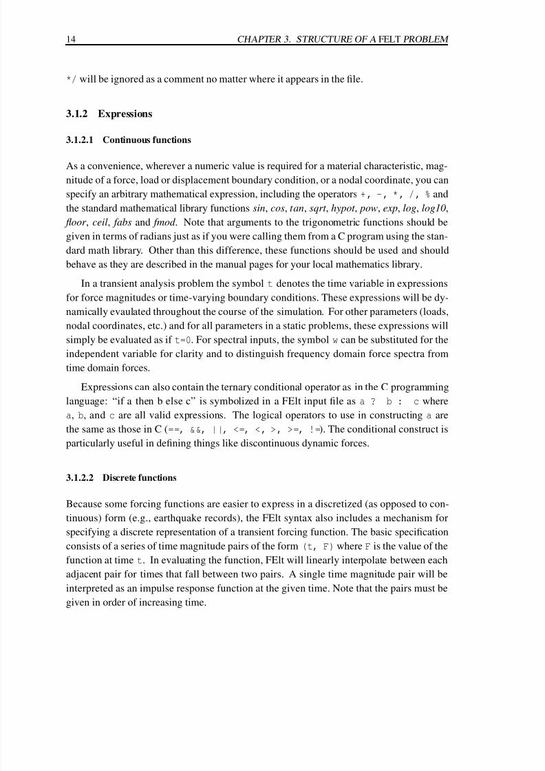
3.1. INPUT FILE SYNTAX 15
You can express a periodic discrete function simply by defining one period and then
entering a + symbol at the end of the expression. You could represent a simple sawtooth
forcing function having a period of 2 seconds and a maximum magnitude of 1000 with an
expression like
forces
sawtooth Fx=(0,0.0) (2,1000.0)+
Figure 3.1 illustrates different ways to define some common types of loading functions with
either continuous or discrete representations.
Figure 3.1: Example loading functions

7/30/2019 Felt Manual
http://slidepdf.com/reader/full/felt-manual 38/236

7/30/2019 Felt Manual
http://slidepdf.com/reader/full/felt-manual 39/236
3.2. SECTIONS OF A FELT INPUT FILE 17
constraints
fixed Tx=C Ty=C Rz=C /* column alignment is unimportant */
free Tx=U Ty=U Rz=U /* I could have used tx, ty and rz */
forces
end_load Fy=-1000
end
3.2 Sections of a FElt input file
3.2.1 Problem description
The problem description section is used to define the problem title and the number of
nodes and elements in the problem. These numbers will be used for error checking so the
specifications given here must match the actual number of nodes and elements given in the
definition sections. Note that the definitions for nodes and elements do not have to be given
in numerical order, as long as nodes 1 ... m and elements 1 ... n (where m is the number
of nodes and n is the number of elements) all get defined in one of the element and node
definition sections in the file. The analysis= statement defines the type of problem that
you wish to solve. Currently it can either be static, transient, static-substitution,
modal, static-thermal, transient-thermal, or spectral. If you do not specify any-
thing, static analysis will be assumed. The problem description section is the only
section which you cannot repeat within a given input file.
3.2.2 Nodes
The nodes section(s) must define all of the nodes given in the problem. Each node must
be located with an x, y, and z coordinate using x=, y=, and z= assignments. Coordinates
are taken as 0.0 if they are not otherwise defined. If a coordinate is left unspecified for a
given node, it takes the value for that coordinate from the previous node. A node must also
have a constraint assigned to it by a constraint= statement. The default constraint leaves
the node completely free in all six degrees of freedom. Like coordinates, if a constraint is
left unspecified, the node will be assigned the same constraint as the previous node. Forces
(applied point loads and moments) on a node are optional and are applied using the force=
statement; if a force is not specified there will be no force applied to that node. You can
also specify an optional lumped mass at a given node with a mass= statement.

7/30/2019 Felt Manual
http://slidepdf.com/reader/full/felt-manual 40/236
18 CHAPTER 3. STRUCTURE OF A FELT PROBLEM
3.2.3 Elements
An element definition section begins with the keywords xxxxx elements where xxxxx is
the symbolic name of a type of element. All elements under this section heading will
be taken to be the given element type. There could be multiple sections that definedbeam elements, but each must begin with the keywords beam elements. If there were
truss elements in the same problem, they would have to be defined in sections which be-
gan with the keywords truss elements. Currently available types are spring, truss,
beam, beam3d, timoshenko, CSTPlaneStrain, CSTPlaneStress, iso2d PlaneStrain,
iso2d PlaneStress, quad PlaneStrain, quad PlaneStress, htk, brick, rod, and
ctg. A FElt problem is not limited to one element type; the routines for assembling the
global stiffness matrix takes care of getting the right parts of the right element stiffness
matrices into the global matrix.
Each element must have a list of nodes to which it is attached. The node list is definedwith the nodes=[ ...] statement. The length of the list inside the square brackets varies
with element type, but must always contain the full number of nodes which the element
type definition requires (see chapter 4 for a complete definition of what each type requires).
A material property must also be assigned to every element with a material= statement.
If the material is never specified, an element will take the same material property as the
previous element. If nothing ever gets assigned to an element, the default material property
will have zeros for all of its characteristics. Chances are this is not what you want. Finally,
an element can have up to three optional distributed loads. Each load is assigned with a
separate load= assignment. Each element type may treat a distributed load differently so
you should be careful that the name given for the loads on a given element match the namesof distributed loads which are defined in a manner conformant with what that element type
is expecting.
3.2.4 Material properties
The material properties section(s) is quite simple. Each material has a name followed
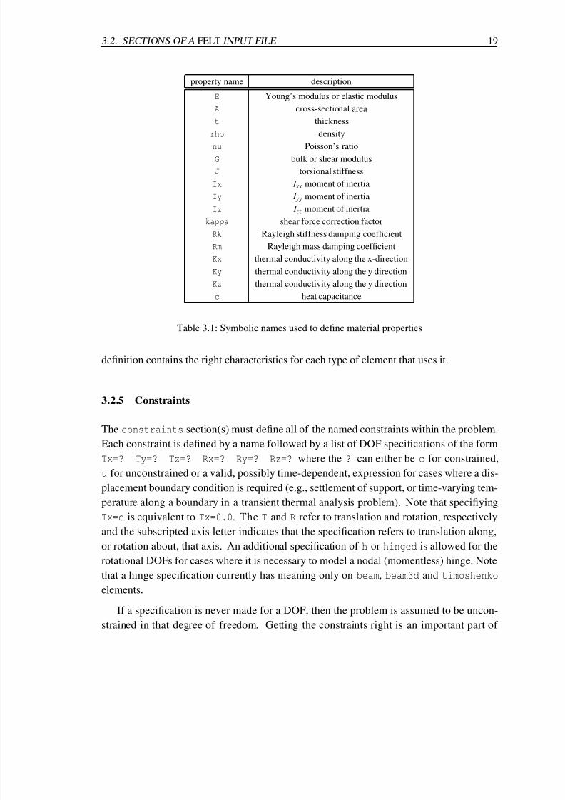
by a list of characteristics. Currently available characteristics are listed in table 3.1.
Note that no element types require a material property with every one of these charac-
teristics defined. In fact, most only use three or four characteristics. You should consult
the element definitions (chapter 4) for a complete list of what each element type requires
from a material property. Density (rho) is always necessary for the materials in a transient,
modal, or spectral analysis problem if you actually want your elements to have any iner-
tia. Different element types can certainly use the same material as long as that material
7/30/2019 Felt Manual
http://slidepdf.com/reader/full/felt-manual 41/236
7/30/2019 Felt Manual
http://slidepdf.com/reader/full/felt-manual 42/236
20 CHAPTER 3. STRUCTURE OF A FELT PROBLEM
getting a reasonable solution out of a finite element problem so you should be aware of
what DOF are active in a given problem (this will depend on which types of elements are
being used ... even in a 2-d problem, the global stiffness matrix will take displacement in
the z direction into account if there are 3-d elements in use, consequently, those displace-
ments should be constrained).
In order to account for initial conditions in transient analysis problems, a constraint
specification may also include the initial (at time t = 0) displacements, and velocity and
acceleration in the translational DOFs. Initial displacements are given with ITx=, IRz=,
etc. You can specify initial accelerations with Ax=, Ay=, and Az=. Initial velocities are
given by Vx=, Vy=, and Vz=. Unspecified velocities and displacements will be taken as 0.0.
If there are no initial accelerations specified (i.e., none of the nodes have a constraint with
an acceleration assigned) then the initial acceleration vector will be solved for by the math-
ematical routines based on the initial force and velocity vectors. If any of the nodes have a
constraint which has an acceleration component defined (even if that component is assignedto 0.0) then the mathematical routines will not solve for an initial acceleration vector; they
will build one based on the constraint information, assigning 0.0 to any component that was
not specified. What this means is that you cannot specify the initial acceleration for only a
few nodes and expect the mathematical routines to simply solve for the rest of them. If you
specify any of the initial accelerations then you are effectively specifying all of them.
3.2.6 Forces
The forces section(s) defines all of the point loads used in the problem and actually looks
a lot like the constraints section. The magnitudes of the forces in the six directions
are specified by Fx=? Fy=? Fz=? Mx=? My=? Mz=?. If the value for a given force
component is not given it is assumed to be zero. The directions for both forces and the
constraints as defined above should be given in the global coordinate system (right-hand
Cartesian).
If you are doing transient analysis, the force definitions can be more complicated than
a simple numerical assignment or expression. FElt allows you to specify a transient force
as either a series of time-magnitude pairs (a discrete function in time) or as an actual con-
tinuous function of time. This latter fact means that you can define a force as Fx=sin(t)rather than having to discretize the sine function. These continuous forcing functions are a
special case of expressions as discussed above.
For spectral analysis problems, you can explicitly specify input spectra using Sfx=,
Smy=, etc. if you want to to compute the actual power spectrum of the output. These

7/30/2019 Felt Manual
http://slidepdf.com/reader/full/felt-manual 43/236
3.2. SECTIONS OF A FELT INPUT FILE 21
Figure 3.2: An example of a complex distributed load.
spectra can be analytic functions of w or discrete frequency, power pairs.
3.2.7 Distributed loads
The distributed loads section(s) must contain a definition for each distributed load
that was assigned in the element definition section(s). A valid definition for a distributed
load is a symbolic name followed by the keywords direction=xxx and values=(n,x)
(m,y) .... The direction assignment must be set to one of parallel, perpendicular,
LocalX, LocalY, LocalZ, GlobalX, GlobalY, GlobalZ, radial, axial. The
valid directions for a given element type, and what those directions refer to for that ele-
ment type are described in the individual element descriptions in chapter 4. The values
assignment is used to assign a list of load pairs to the named load. A load pair is given
in the form (n, x) where n is the local node number to which the magnitude given by xapplies. Generally, two pairs will be required after the values= token. The imaginary line
between the two magnitudes at the two nodes defines an arbitrarily sloping linearly distrib-
uted load. This allows you to specify many common load shapes: a constant distributed
load of magnitude y, including cases of self-weight, a load which slopes from zero at one
node to x at a second node, or a linear superposition of these two cases in which the load
has magnitude y at node 1 and magnitude x + y at node 2. This latter case is illustrated in
figure 3.2. The definition of this load would be
distributed loads
load_case_1 direction=perpendicular values=(1,-2000) (2,-6000)
In the future, higher-order load shapes may be supported by some elements and thus
require the specification of more than two load pairs.

7/30/2019 Felt Manual
http://slidepdf.com/reader/full/felt-manual 44/236

7/30/2019 Felt Manual
http://slidepdf.com/reader/full/felt-manual 45/236
3.3. AN ILLUSTRATED EXAMPLE 23
parameter description example r/o
start frequency range start (SP), load range start (LR) 0.0 r
stop time- (T, TT), frequency- (SP) or load- (LR) range end 10.0 r
step time- (T, TT), frequency- (SP) or load- (LR) step 0.05 r
alpha α in HHT-α and transient thermal integration (T, TT) 0.5 o
gamma γ in HHT-α integration (T) 0.25 o
beta β in HHT-α integration (T) 0.5 omass-mode element mass matrices to use (T, TT, SP, M) lumped r
nodes list of nodes for which you want results (T, TT, SP, LR, LC) [1,4,5] r
dofs list of DOF at each result node (T, TT, SP, LR, LC) [Tx, Rz] r
Rk global Rayleigh damping constant for stiffness (T, M, SP) 3.0 o
Rm global Rayleigh damping constant for mass (T, M, SP) 1.4 o
input-node node to be parametrically excited (LR) 4 r
input-dof DOF at the input node to be excited (LR) Ty r
tolerance convergence tolerance (SUB) 1e-3 r
iterations maximum permitted number of iterations (SUB) 100 r
relaxation under- (over-) relaxation factor (SUB) 0.8 r
load-steps number of incremental steps to full load (SUB) 10 r
Table 3.2: Meaning given to the various analysis parameters. T indicates transient analysis; TT
is transient-thermal; SP is spectral; M is modal; LR is static analysis (linear or nonlinear) with
load ranges; LC is static analysis (linear or nonlinear) with load cases; SUB is non-linear static
substitution analysis. The r/o column indicates whether the parameter is (r)equired for the given
analyses or if the (o)ptional default value of 0.0 will be used if nothing is specified.

7/30/2019 Felt Manual
http://slidepdf.com/reader/full/felt-manual 46/236
24 CHAPTER 3. STRUCTURE OF A FELT PROBLEM
Figure 3.3: A mixed element problem with distributed loads.
problem description
title="Mixed Element Sample" nodes=4 elements=3
nodes
1 x=0 y=0 constraint=pin
2 x=6 y=0 constraint=free
3 x=12 y=0 constraint=roller
4 x=6 y=-10 constraint=fixed
beam elements
1 nodes=[1,2] material=steel load=left_side
2 nodes=[2,3] load=right_side
truss elements
3 nodes=[2,4] material=spring
material properties
steel A=1 E=210e9 Ix=4e-4
spring A=4.76e-7 E=210e9 /* k = 10 kN/m */
constraints
pin Tx=c Ty=c Tz=c Rz=u /* we better constrain Tz because */
free Tx=u Ty=u Tz=c Rz=u /* there is a truss element! */
roller Tx=u Ty=c Tz=c Rz=u
fixed Tx=c Ty=c Tz=c Rz=c

7/30/2019 Felt Manual
http://slidepdf.com/reader/full/felt-manual 47/236

7/30/2019 Felt Manual
http://slidepdf.com/reader/full/felt-manual 48/236
26 CHAPTER 3. STRUCTURE OF A FELT PROBLEM
analysis parameters
dt=0.05 duration=0.8
beta=0.25 gamma=0.5 alpha=0.0
nodes=[8] dofs=[Tx] mass-mode=lumped
nodes
1 x=0 y=0 constraint=fixed
2 x=360 y=0
3 x=0 y=180 constraint=free force=f1
4 x=360
5 x=0 y=300 force=f2
6 x=360
7 x=0 y=420 force=f3
8 x=360
beam elements
1 nodes=[1,3] material=wall_bottom
2 nodes=[3,5] material=wall_top
3 nodes=[5,7]
4 nodes=[7,8] material=floor_top load=top_wt
5 nodes=[5,6] material=floor_bottom load=bottom_wt
6 nodes=[3,4] load=bottom_wt
7 nodes=[8,6] material=wall_top
8 nodes=[6,4]
9 nodes=[4,2] material=wall_bottom
material propertieswall_bottom A=13.2 Ix=249 E=30e6 rho=0.0049 /* rho is in lb-sˆ2/inˆ4 */
wall_top A=6.2 Ix=107 E=30e6 rho=0.0104
floor_top A=12.3 Ix=133 E=30e6 rho=0.01315
floor_bottom A=24.7 Ix=237 E=30e6 rho=0.0136
distributed loads
top_wt direction=perpendicular values=(1,-62.5) (2,-62.5)
bottom_wt direction=perpendicular values=(1,-130) (2,-130)
forces
f1 Fx=1000*(t < 0.2 ? 25*t : 5)f2 Fx=800*(t < 0.2 ? 25*t : 5)
f3 Fx=500*(t < 0.2 ? 25*t : 5)
constraints
fixed Tx=c Ty=c Rz=c
7/30/2019 Felt Manual
http://slidepdf.com/reader/full/felt-manual 49/236
3.5. FORMAT CONVERSION 27
free Tx=u Ty=u Rz=u
end
3.5 Format conversion
Any problem that you want to solve with FElt must be formatted according to the rules that
we have just described. However, we recognize that there are countless other formats that
provide for descriptions of these same kinds of problems (at least the geometric aspects of
the problem). Because of this, FElt provides a mechanism for translating back and forth
between FElt and alternative syntaxes.
3.5.1 Conversion basics
A common example of a popular geometric description syntax is DXF (drawing inter-
change format). DXF files can be produced by any number of CAD and geometric mod-
eling programs. The FElt conversion tool, patchwork , can translate DXF files to and from
the FElt syntax. patchwork is invoked with a command-line like:
% patchwork -dxf bridge.dxf -felt bridge.flt
This example would convert the geometric description given in the file bridge.dxf to
the geometric basics of a standard FElt file, bridge.flt. Geometric basics in this case
means that only the nodes and elements sections will be translated; the DXF file cannot
contain any information about material properties, forces, loads, constraints, and therefore
this information will be left incomplete in the resulting FElt file.
patchwork can also translate FElt files into other formats. You might want to do this if
you had used some of FElt’s mesh generation capabilities for the bulk of your geometricproblem description, but wanted to do some refinement using your favorite CAD program.
The patchwork command line to do something like that is simply the reverse of above:
% patchwork -felt mesh.flt -dxf mesh.dxf
7/30/2019 Felt Manual
http://slidepdf.com/reader/full/felt-manual 50/236
28 CHAPTER 3. STRUCTURE OF A FELT PROBLEM
3.5.2 patchwork details
patchwork operates by providing routines to read and write the different file formats based
around a single data structure. The input formatted file is translated into the uniform
database and then the output formatted file is generated from this same database. Theability to read or write any given format is dependent on whether or not routines exist to go
back and forth between the file syntax and the uniform data structure. Currently, patchwork
can read (i.e., the allowable input formats are) DXF files, standard FElt files, and data files
formatted for use in graphing applications like gnuplot ; patchwork can write (i.e., allow-
able output formats are) FElt, DXF, gnuplot , and files formatted for the software that is
distributed with Logan’s introductory finite element text [13]. Capabilities for additional
formats will be added as time permits and demand warrants. Note that the DXF handling
routines are limited to line and polygonal polyline entities.
When invoking patchwork , the input format and file always come first. The syntax ispatchwork -[iformat] ifile -[oformat] ofile, where [iformat] can currently be
one of dxf, felt, graph and [oformat] can be one dxf, felt, graph, logan. An
input or output file name of - (a hyphen) indicates that input should be read from standard
input and/or output should be written to standard output, respectively.

7/30/2019 Felt Manual
http://slidepdf.com/reader/full/felt-manual 51/236
Chapter 4
The FElt Element Library
4.1 Introduction
The FElt element library contains line, plane and solid elements. Line elements in-
clude a one-dimensional spring (spring), a bar or truss element (truss), two- and three-
dimensional Euler-Bernoulli beams (beam and beam3d), and a two-dimensional beam based
on Timoshenko theory, (timoshenko). The set of planar elements consists of constant
strain triangles (CSTPlaneStrain and CSTPlaneStress), isoparametric quadrilaterals
(iso2d PlaneStress, iso2d PlaneStrain, quad PlaneStrain, quad PlaneStress)
and an HTK plate bending element (htk). The only solid element in the library is an
eight node brick (brick). There is an axisymmetric triangular element (axisymmetric).
The only elements available for thermal analysis are a simple one-dimensional line element
(rod) and a constrant temperature gradient triangular element (ctg). In the above list, the
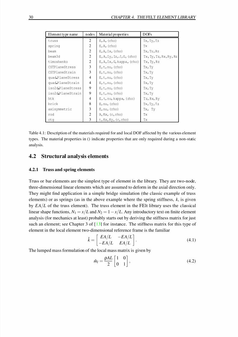
names in parentheses indicate the actual symbolic type names of the elements.
The number of nodes and the material properties needed for defining each element and
the DOF that the element affects are summarized in the table below. A brief description
for each element follows the table; detailed derivations of element stiffness matrices can be
found in any number of finite element textbooks.
29
7/30/2019 Felt Manual
http://slidepdf.com/reader/full/felt-manual 52/236
30 CHAPTER 4. THE FELT ELEMENT LIBRARY
Element type name nodes Material properties DOFs
truss 2 E,A,(rho) Tx,Ty,Tz
spring 2 E,A,(rho) Tx
beam 2 E,A,Ix,(rho) Tx,Ty,Rz
beam3d 2 E,A,Iy,Iz,J,G,(rho) Tx,Ty,Tz,Rx,Ry,Rz
timoshenko 2 E,A,Ix,G,kappa,(rho) Tx,Ty,Rz
CSTPlaneStress 3 E,t,nu,(rho) Tx,Ty
CSTPlaneStrain 3 E,t,nu,(rho) Tx,Ty
quad PlaneStress 4 E,t,nu,(rho) Tx,Ty
quad PlaneStrain 4 E,t,nu,(rho) Tx,Ty
iso2d PlaneStress 9 E,t,nu,(rho) Tx,Ty
iso2d PlaneStrain 9 E,t,nu,(rho) Tx,Ty
htk 4 E,t,nu,kappa,(rho) Tz,Rx,Ry
brick 8 E,nu,(rho) Tx,Ty,Tz
axisymmetric 3 E,nu,(rho) Tx, Ty
rod 2 A,Kx,(c,rho) Tx
ctg 3 t,Kx,Ky,(c,rho) Tx
Table 4.1: Description of the materials required for and local DOF affected by the various element
types. The material properties in () indicate properties that are only required during a non-static
analysis.
4.2 Structural analysis elements
4.2.1 Truss and spring elements
Truss or bar elements are the simplest type of element in the library. They are two-node,
three-dimensional linear elements which are assumed to deform in the axial direction only.
They might find application in a simple bridge simulation (the classic example of truss
elements) or as springs (as in the above example where the spring stiffness, k , is given
by EA/ L of the truss element). The truss element in the FElt library uses the classical
linear shape functions, N 1 = x/ L and N 2 = 1− x/ L. Any introductory text on finite element
analysis (for mechanics at least) probably starts out by deriving the stiffness matrix for just
such an element; see Chapter 3 of [13] for instance. The stiffness matrix for this type of
element in the local element two-dimensional reference frame is the familiar
k =
EA/ L − EA/ L− EA/ L EA/ L
. (4.1)
The lumped mass formulation of the local mass matrix is given by
ml =ρ AL
2
1 0
0 1
, (4.2)

7/30/2019 Felt Manual
http://slidepdf.com/reader/full/felt-manual 53/236
4.2. STRUCTURAL ANALYSIS ELEMENTS 31
and the consistent mass formulation by
mc =ρ AL
6
2 1
1 2
. (4.3)
The 2 ×2 matrices in local element coordinates are transformed into the global coordi-nate system (and into 6 × 6 form) according to
k = T TkT , (4.4)
where the transformation matrix is given by
T =
cosθ x cosθ y cosθ z 0 0 0
0 0 0 cosθ x cosθ y cosθ z
. (4.5)
The direction cosines are simply the projections of the local coodinate axes onto the global
coordinate axes,
cosθ x =x1 − x2
L, (4.6)
cosθ y =y1 − y2
L, (4.7)
cosθ z =z1 − z2
L. (4.8)
The stress calculated for truss elements is the axial stress (not load). A positive quantity
indicates tension, negative indicates compression. If a distributed load is assigned to a truss
element it is assumed to be a linearly distributed axial loading condition (i.e., it must be
directed parallel). Nothing else makes much sense since a truss element cannot carry
bending or shear forces along its length. The sign convention for the magnitude of the load
pairs is positive for loads pointing from local node 1 to local node 2.
The spring element included in FElt is simply the truss element described above without
the transformation from local element coordinates to global coordinates. What this means
is that the element matrices are only 2 × 2 and because of this they must be defined only
along the global x-axis. Distributed loads are not supported by spring elements.
4.2.2 Euler-Bernoulli beam elements
4.2.2.1 Special case two-dimensional element
A beam element is a two-dimensional, two-node linear element which can carry in-plane
axial, shear and bending forces. The moment of inertia used in stiffness calculations (spec-
ified with Ix) is the bending moment of inertia about the cross-section x-x axis (which in
7/30/2019 Felt Manual
http://slidepdf.com/reader/full/felt-manual 54/236
32 CHAPTER 4. THE FELT ELEMENT LIBRARY
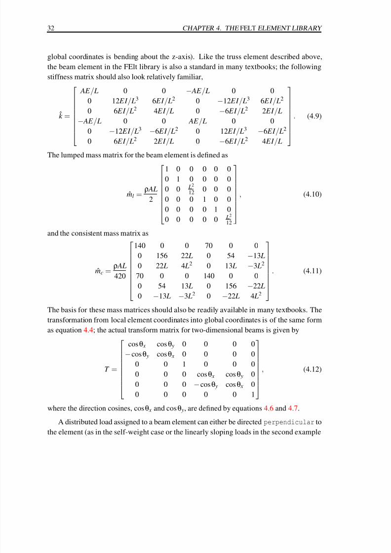
global coordinates is bending about the z-axis). Like the truss element described above,
the beam element in the FElt library is also a standard in many textbooks; the following
stiffness matrix should also look relatively familiar,
k =
AE / L 0 0
− AE / L 0 0
0 12 EI / L3 6 EI / L2 0 −12 EI / L3 6 EI / L2
0 6 EI / L2 4 EI / L 0 −6 EI / L2 2 EI / L
− AE / L 0 0 AE / L 0 0
0 −12 EI / L3 −6 EI / L2 0 12 EI / L3 −6 EI / L2
0 6 EI / L2 2 EI / L 0 −6 EI / L2 4 EI / L
. (4.9)
The lumped mass matrix for the beam element is defined as
ml =ρ AL
2
1 0 0 0 0 0
0 1 0 0 0 0
0 0 L2
120 0 0
0 0 0 1 0 0
0 0 0 0 1 0
0 0 0 0 0 L2
12
,(4.10)
and the consistent mass matrix as
mc =ρ AL
420
140 0 0 70 0 0
0 156 22 L 0 54 −13 L
0 22 L 4 L2 0 13 L −3 L2
70 0 0 140 0 0
0 54 13 L 0 156−
22 L
0 −13 L −3 L2 0 −22 L 4 L2
. (4.11)
The basis for these mass matrices should also be readily available in many textbooks. The
transformation from local element coordinates into global coordinates is of the same form
as equation 4.4; the actual transform matrix for two-dimensional beams is given by
T =
cosθ x cosθ y 0 0 0 0
−cosθ y cosθ x 0 0 0 0
0 0 1 0 0 0
0 0 0 cosθ x cosθ y 0
0 0 0 −cosθ y cosθ x 00 0 0 0 0 1
, (4.12)
where the direction cosines, cosθ x and cosθ y, are defined by equations 4.6 and 4.7.
A distributed load assigned to a beam element can either be directed perpendicular to
the element (as in the self-weight case or the linearly sloping loads in the second example

7/30/2019 Felt Manual
http://slidepdf.com/reader/full/felt-manual 55/236
4.2. STRUCTURAL ANALYSIS ELEMENTS 33
Figure 4.1: Sign convention for local forces on a beam element.
above), parallel to the element (just like a linearly distributed axial load in the truss
case), or in the GlobalX or GlobalY directions. Note that loads given in the LocalY and
LocalX directions will be taken as equivalent to the perpendicular and parallel cases,respectively. For perpendicular loads a positive magnitude indicates that the load points
in the direction of positive ˆ y. A positive parallel loads point from node 1 to node 2 as in
the truss case. Similarly, the sign convention for loads in the global directions follow the
sign convention of the global coordinate axes. Each beam element is limited to two applied
distributed loads.
After displacements are found, six internal force quantities are computed for each beam
element. These quantities are the axial force, shear force and bending moment at both
nodes. The sign convention for these forces is shown in Figure 4.1. This convention is
based on a coordinate system in which the local x-axis, ˆ x
, points from node 1 to node 2. As z and ˆ z always coincide for the 2d beam element, and we define the positive z-axis to point
out of the page, ˆ y = z × ˆ x.
The three beam type elements (beam, beam3d and timoshenko) all are capable of re-
solving hinged boundary conditions for the rotational degrees of freedom. The adjustment
is made to the element stiffness matrix in global coordinates according to the following
procedure. Given a hinged DOF, do f , then for all entries in k (the element stiffness matrix)
not associated with do f (all entries not in row or column do f ),
k (i, j) = k (i, j)−
k (do f , j)
k (do f ,do f )
k (i,do f ). (4.13)
The inherent problem in this method of dealing with hinged conditions is that we cannot
calculate any displacements associated with the hinged DOF and thus, the internal forces
calculated for any element with a hinged node will not be correct. Displacements other
than at the hinged DOF will be accurate.
7/30/2019 Felt Manual
http://slidepdf.com/reader/full/felt-manual 56/236
34 CHAPTER 4. THE FELT ELEMENT LIBRARY
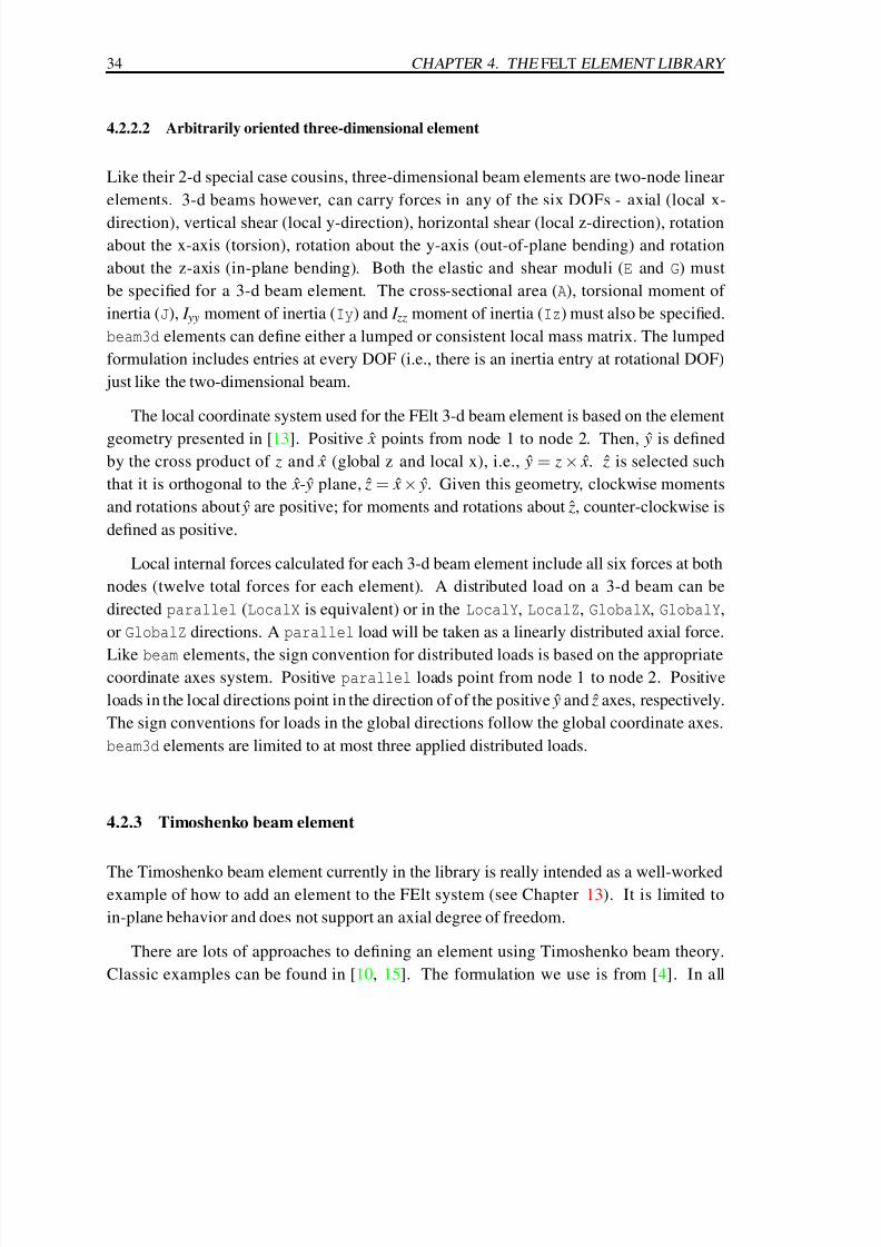
4.2.2.2 Arbitrarily oriented three-dimensional element
Like their 2-d special case cousins, three-dimensional beam elements are two-node linear
elements. 3-d beams however, can carry forces in any of the six DOFs - axial (local x-
direction), vertical shear (local y-direction), horizontal shear (local z-direction), rotation
about the x-axis (torsion), rotation about the y-axis (out-of-plane bending) and rotation
about the z-axis (in-plane bending). Both the elastic and shear moduli (E and G) must
be specified for a 3-d beam element. The cross-sectional area (A), torsional moment of
inertia (J), I yy moment of inertia (Iy) and I zz moment of inertia (Iz) must also be specified.
beam3d elements can define either a lumped or consistent local mass matrix. The lumped
formulation includes entries at every DOF (i.e., there is an inertia entry at rotational DOF)
just like the two-dimensional beam.
The local coordinate system used for the FElt 3-d beam element is based on the element
geometry presented in [13]. Positive ˆ x points from node 1 to node 2. Then, ˆ y is definedby the cross product of z and ˆ x (global z and local x), i.e., ˆ y = z × ˆ x. ˆ z is selected such
that it is orthogonal to the ˆ x- ˆ y plane, ˆ z = ˆ x × ˆ y. Given this geometry, clockwise moments
and rotations about ˆ y are positive; for moments and rotations about ˆ z, counter-clockwise is
defined as positive.
Local internal forces calculated for each 3-d beam element include all six forces at both
nodes (twelve total forces for each element). A distributed load on a 3-d beam can be
directed parallel (LocalX is equivalent) or in the LocalY, LocalZ, GlobalX, GlobalY,
or GlobalZ directions. A parallel load will be taken as a linearly distributed axial force.
Like beam elements, the sign convention for distributed loads is based on the appropriatecoordinate axes system. Positive parallel loads point from node 1 to node 2. Positive
loads in the local directions point in the direction of of the positive ˆ y and ˆ z axes, respectively.
The sign conventions for loads in the global directions follow the global coordinate axes.
beam3d elements are limited to at most three applied distributed loads.
4.2.3 Timoshenko beam element
The Timoshenko beam element currently in the library is really intended as a well-workedexample of how to add an element to the FElt system (see Chapter 13). It is limited to
in-plane behavior and does not support an axial degree of freedom.
There are lots of approaches to defining an element using Timoshenko beam theory.
Classic examples can be found in [10, 15]. The formulation we use is from [4]. In all

7/30/2019 Felt Manual
http://slidepdf.com/reader/full/felt-manual 57/236
4.2. STRUCTURAL ANALYSIS ELEMENTS 35
formulations, the stiffness matrix is defined as
k =EI
(1
+φ
) L3
12 6 L −12 6 L
6 L (4 +φ) L2 −6 L (2 −φ) L2
−12
−6 L 12
−6 L
6 L (2 −φ) L2 −6 L (4 +φ) L2
. (4.14)
In the above equation, φ is defined as the ratio of the bending stiffness to shear stiffness,
φ =EI
κ GA. (4.15)
κ is the shear coefficient from Timoshenko beam theory. Cowper [2] provides an approxi-
mation for κ based on Poisson’s ratio,
κ =10(1 + ν)
12 + 11 ν, (4.16)
if a better estimate is not available. This approximation will automatically be assumed if
you provide nu rather than kappa in the material property for a Timoshenko beam element.
Because there is no axial DOF in this formulation, you need to be careful about horizontally
oriented elements; nothing will be assembled into the translational x DOF in these cases so
you should be extra careful about constraints. The lumped mass matrix for the timoshenko
element looks just like that for the 2-d Euler-Bernoulli element (eq. 4.10), minus the axial
DOF of course. The definition of the consistent mass matrix varies from one formulation
of Timoshenko theory to the next. The definition in the formulation that we are using is
considerably more complicated than the Euler-Bernoulli formulation; see [4] for details.
Distributed loads on timoshenko elements can only be directed in the perpendicular
(equivalent to LocalY) direction. (There are no axial DOF after all). The sign conventions
for these loads and for internal forces is the same as that for the standard beam element.
The internal forces calculated will be the shear forces and bending moment at each end.
4.2.4 Constant Strain Triangular (CST) elements
Two different CST elements are in the FElt library - one for plane stress analysis and
one for plane strain analysis. This means that the only difference between the two is that
the constitutive matrix, D, used in the element stiffness formulation is different for the
two cases. A CST element is a three-node, two-dimensional, planar element. Each CST
element should exist completely in a single x-y plane. The node numbers must be assigned
to a CST element in counter-clockwise order to avoid the element having a negative area.

7/30/2019 Felt Manual
http://slidepdf.com/reader/full/felt-manual 58/236
36 CHAPTER 4. THE FELT ELEMENT LIBRARY
The lumped mass matrix for a CST element is formed simply by dividing the mass of
the element equally between the three nodes, i.e.,
ml =ρ At
3
1 0 0 0 0 0
0 1 0 0 0 0
0 0 1 0 0 0
0 0 0 1 0 0
0 0 0 0 1 0
0 0 0 0 0 1
, (4.17)
where A is the computed planar area of the element (not the area as defined by the material
property A=). There is no consistent mass formulation available for the current set of CST
elements.
Six stress quantities are computed for each CST element: σ x, σ y, τ xy, σ1, σ2, θ, where
σ x, σ y, τ xy, are the stresses in the global coordinate system, σ1, σ2 are the principal streses,and θ is the orientation of the principal stress axis. A distributed load on a CST element is
taken as an in-plane surface traction. Valid directions for loads are GlobalX and GlobalY.
The sign convention for load magnitude follows the orientation of the global axes. Loads
which are perpendicular or parallel to element sides which are not parallel to one of the
global axes must be broken down into components which are parallel to the axes and then
specified as two separate loads.
4.2.5 Two-dimensional isoparametric elements
4.2.5.1 General four to nine node element
Like CST elements, isoparametric elements are available for either plane strain or plane
stress analysis. Isoparametric elements are 2-d planar, quadrilateral elements with nine
nodes. Any of the last five nodes are optional, however and the fourth node can be the third
node repeated. The numbering convention is shown in Figure 4.2. If any of nodes 5 - 9 are
left out, their place must be filled with a zero in the nodes=[ ...] specification for that
element (i.e. you must always specify nine numbers, it is simply that any or all of the last
five might be specified as zero). None of the first four nodes can be zero. If the fourth and
third nodes are the same, then the element will be degenerated to a triangle. In this casenodes 5 - 9 must be zero.
Currently, no stresses are computed for the generalized isoparametric element. Dis-
tributed loads on the generalized isoparametric element are ignored and do not affect the
problem solution in any way.

7/30/2019 Felt Manual
http://slidepdf.com/reader/full/felt-manual 59/236
4.2. STRUCTURAL ANALYSIS ELEMENTS 37
Figure 4.2: Node numbering scheme for nine node isoparametric planar element.
4.2.5.2 Simple four node element
quad PlaneStress and quad PlaneStrain elements are just like the generalized isopara-
metric elements described above, but they can only have the first four nodes. They are
intended to make problem definition easier in cases where the added accuracy that the ad-
ditional nodes offer is not worth the extra effort. Like the generalized case, if the fourth
node is the same as the third node the element will be degenerated into a triangle. This
allows for easy mixing and matching of element shapes without changing element types
(though this too would be allowed).
Distributed loads on the four node isoparametric elements work exactly as they do in
the CST case. The stresses computed for each four node isoparametric are also the same as
those computed for CSTs.
Like CST elements, only a lumped mass formulation is available for the mass matrices
of isoparametric quadrilateral elements. The lumped formulation is generated by lumping
the total mass of the element equally at the four nodes (or the three nodes if the element is
being degenerated into a triangle).
4.2.6 Plate bending element
The plate bending element in FElt is a simple four node isoparametric quadrilateral that
uses selective reduced integration to prevent shear locking. The classic reference for this

7/30/2019 Felt Manual
http://slidepdf.com/reader/full/felt-manual 60/236
38 CHAPTER 4. THE FELT ELEMENT LIBRARY
Figure 4.3: Sign convention for force resultants on an htk element.
approach is [10]. The effect is achieved simply by using one-point Gaussian quadrature to
under-integrate the shear contribution to the stiffness where two-point quadrature is used
on the bending contributions.
htk elements must exist entirely in the x-y plane; the three DOF at each node each
represent out of plane deformation. Rotations are positive in the right-hand sense. You can
generate plate bending triangular elements by using htk elements with the third and fourth
nodes being equal (just like you can generate triangles from isoparametric quadrilateral
elements). Mass matrices for htk elements also work the exact same way as the mass
matrices for the in-plane quad PlaneStress and quad PlaneStrain elements.
Figure 4.3 illustrates the sign convention for the internal force resultants calculated for
each htk element.

7/30/2019 Felt Manual
http://slidepdf.com/reader/full/felt-manual 61/236
4.2. STRUCTURAL ANALYSIS ELEMENTS 39
Figure 4.4: An example of valid node ordering on a brick element.
4.2.7 Solid brick element
The eight-node solid brick element in FElt is based on an isoparametric formulation using
linear shape functions. The element incorporates all three translational DOF at each node
for a total of 24 local degrees of freedom. The 24×24 element stiffness matrix is evaluated
using a fourth-order accurate 2 × 2 × 2 Gaussian quadrature rule. This formulation results
in stress calculations at eight integration points. Figure 4.4 shows the local node number-
ing convention for bricks. As the figure illustrates, nodes 1-4 and nodes 5-8 must define
opposite faces.
All six independent components of the stress tensor are calculated for brick elements.
Brick elements are still somewhat limited, however, in that distributed loads are not handled
and element definition routines do not calculate a mass matrix. Also, note that because
brick elements are the only solid elements in the FElt library, they are also the only elements
which are not fully supported by velvet , both in terms of problem definition and in terms of
post-processing.

7/30/2019 Felt Manual
http://slidepdf.com/reader/full/felt-manual 62/236
40 CHAPTER 4. THE FELT ELEMENT LIBRARY
4.2.8 Axisymmetric elements
The axisymmetric element is a three node triangular element based on linear shape func-
tions. The axis of symmetry/revolution is always the y-axis. Distributed loads can be
directed in either the axial (y) or radial (x) directions.
4.3 Thermal analysis elements
Thermal elements only have one degree of freedom per node, the nodal temperature. Pre-
scribed and initial temperatures are assigned using constraints, Tx=, and iTx=. Heat sources
are specified using nodal forces (Fx=). For uniform heat sources, simply apply the same
force to all nodes.
4.3.1 Rod element
The rod element is a two node straight line element for thermal analysis. Convection sur-
faces are specified using distributed loads. The direction of the load does not matter and
does not need to be specified. The node, magnitude pairs of the values definition of the
load are used to specify the surface on which the convection is taking place and the con-
vection coefficient and free stream temperature. For example values=(1,20) (2,50)
specifies a convection coefficient of 20, a free stream temperature of 50, and that the con-
vection acts over the circumferential surface area of the rod. If the node values are equal in
the two pairs then the convecting surface is taken to be an exposed end of the rod.
4.3.2 Constant Temperature Gradient (CTG) element
The ctg element is a thermal analog to the CST triangular elements for mechanical prob-
lems. The temperature is assumed to vary linearly over the element. As with rod elements,
convection on ctg elements is specified using distributed loads. Only the three edges are
handled. The node, magnitude pairs of the values definition of the load are used to specify
the edge on which the convection is taking place and, as for the rod, the convection coef-
ficient and free stream temperature. For a ctg element the definition values=(1,20)(2,50) specifies a convection coefficient of 20, a free stream temperature of 50, and that
the convection acts on the edge defined by local element node numbers 1 and 2.

7/30/2019 Felt Manual
http://slidepdf.com/reader/full/felt-manual 63/236
Chapter 5
The felt Application
5.1 Using felt
The basic way to solve a problem with felt is simply to type felt foo.flt on the com-
mand line, where foo.flt is the name of a FElt input file. There are several command line
options, however, which offer additional capabilities.
-version display the current version number of felt and exit.
-help display a brief help message which lists all of the available command line
options.
-debug will generate a FElt file, that if all is working well, should look exactly like
the original input file. The generated file represents what the application
thinks it was given.
-preview produces an ASCII rendering of the problem geometry. The graphics may
not be great but the result is often good enough for a simple sanity check.
-renumber will invoke a Gibbs-Poole-Stockmeyer/Gibbs-King automatic node renum-
bering algorithm for bandwidth/profile reduction of the global stiffness ma-
trix (and mass and damping matrices in transient analysis). The renumber-ing will only affect solution time and memory requirements; results will be
referenced to the originally assigned node numbers. Generally there is no
benefit in using this capability for problems with small numbers of nodes.
+table disables tabular output for transient and spectral analysis problems.
41
7/30/2019 Felt Manual
http://slidepdf.com/reader/full/felt-manual 64/236
42 CHAPTER 5. THE FELT APPLICATION
-plot generates an ASCII character based plot (or plots) of results for transient or
spectral analysis problems.
-transfer only calculate the transfer functions during spectral analysis. The output
can be graphical and/or tabular depending on the plot and table options.
-eigen in a modal analysis problem, only calculate the eigenvalues (natural fre-
quencies) and eigenvectors (mode shapes) before quitting (i.e., do not cal-
culate modal mass, damping and stiffness matrices).
-orthonormal
use orthonormal mode shapes to calculate modal mass, damping, and stiff-
ness matrices in a modal analysis problem.
-matrices will print the global matrices that are appropriate to this problem. In static
analysis this would simply be the stiffness matrix; in transient analysis thisis the stiffness, damping, and mass matrices; in modal analysis, this is the
condensed stiffness, damping, and mass matrices.
-summary will generate a summary of all the material properties that were used in the
problem. The number of elements using a material, total length, surface area
and mass of that material (if masses are desired, then the material properties
definition must include a density) and the total mass of the structure are
given.
-graphics foo1will create a graphics file called foo1 so the user can visualize the structure
with a standard graphing package to make sure that everything is connected
where it should be. The format of this file will be a list of coordinate triplets
connecting each element, with blank lines delimiting the end of an element.
-cpp filename
substitute filename for the pre-processor to run on the input file.
-nocpp do not run the input file through the pre-processor.
-Idirectory
add directory to the standard search path for include files in the pre-
processor.
-Uname undefine the macro name in the pre-processor.

7/30/2019 Felt Manual
http://slidepdf.com/reader/full/felt-manual 65/236
5.1. USING FELT 43
-Dname=value
define name to be the macro value in the pre-processor.
Additionally, every FElt file that is run through felt is pre-processed by the C preproces-sor (except in DOS). This allows for the use of macro definitions and include files within
a FElt input file. An example of this capability is the international translation files which
allow you to specify a FElt input file in a language other than English. These translation
files are nothing more than include files which contain #define statements which map the
non-English terms to what FElt actually expects (the regular English terms). An input file
that takes advantage of these powerful features might look like this:
#include "german.trn"
#define map(x) ((x)*(cos((x))*cos((x)) + sin((x))*sin((x))))
problembeschreibung
titel="A cantilever beam" knoten=3 elemente=2
knoten
1 x=0 y=0 krafte=point_load zwangsbedingung=pin
2 x=map(240) y=0
beam elemente
1 knoten=[1,2] material=steel
materialeigenschaften
steel e=30e6 ix=100 a=10
kraefte
point_load fy=-1000
zwangsbedingungen
pin tx=c ty=c rz=u
ende
The C preprocessor options and capabilities are described more fully in the felt (1fe) manual
page. The international translation capability is discussed more fully (including current
translation tables) in appendix A.

7/30/2019 Felt Manual
http://slidepdf.com/reader/full/felt-manual 66/236
44 CHAPTER 5. THE FELT APPLICATION
5.2 Solving a problem
As mentioned above the easiest way to solve a problem is to simply do
% felt foo.flt
at the shell prompt . If you want to save the output it is easy to simply re-direct standard
output to a file by doing
% felt foo.flt > foo.results
Th file foo.results could then be printed using whatever printer facilities exist at your
site (lp, lpr , print , etc.) If you want to plot the structure, the command line might look like
this:
% felt -graphics foo.graph foo.flt > foo.results
% myplotter foo.graph
The file foo.graph could then be used with a program like gnuplot , xmgr or xgraph (here
we used a mystical program called myplotter ) to visualize the structure and make sure that
all the elements were connected properly.
5.3 Interpreting the output from felt
The output from felt is the most basic form of output that all applications in the FElt system
produce. That is, no matter how you specify and solve a FElt problem (either with felt or
velvet ) the basic output will look the same.
The main output will vary depending on the analysis type defined in the input file.
In addition to the results from the specific analysis, supplemental kinds of output which
are available include material usage statistics, debugging information, and print-outs of
the global stiffness and mass matrices. Supplemental output from felt is controlled via
command line switches (see section 5.1).
5.3.1 Static analysis
For a static analysis problem there are three sections of output: nodal displacements, ele-
ment stresses and reaction forces. The nodal displacements are given in a table with the six

7/30/2019 Felt Manual
http://slidepdf.com/reader/full/felt-manual 67/236
5.3. INTERPRETING THE OUTPUT FROM FELT 45
global DOF running across the top and the list of nodes going down. The displacement of
each node in each DOF is printed. Of course in most problems not all DOF will be active
so many of the displacements will simply come up as zero.
The information in the element stress table will vary depending on the element type.
Each row contains up to six columns of information; if an element calculates more than six
stresses or loads, the information for that element will take up more than one row (beam3d
elements for instance have 12 loads calculated and thus the information for each element
takes up two rows). The output format for each element type is summarized in Table 5.1.
Element col 1 col 2 col 3 col 4 col 5 col 6
truss σ x
beam f 1 x f 1 y m1 z f 2 x f 2 y m2
z
beam3d f 1 x f 1 y f 1 z m1 x m1
y m1 z
f 2 x f 2 y f 2 z m2 x m2
y m2 z
timoshenko f 1 y m1 z f 2 y m2
z
CSTPlaneStress σ x σ y τ xy σ1 σ2 θ
CSTPlaneStrain σ x σ y τ xy σ1 σ2 θ
quad PlaneStress σ1 x σ1
y τ1 xy σ1
1 σ12 θ1
......
......
......
σ4 x σ4
y τ4 xy σ4
1 σ42 θ4
quad PlaneStrain σ1 x σ1
y τ1 xy σ1
1 σ12 θ1
......
......
......
σ4 x σ4
y τ4 xy σ4
1 σ42 θ4
htk m xx m yy m xy q x q y
brick σ1 xx σ1
yy σ1 zz τ1
xy τ1 yz τ1
zx...
......
......
...
σ8 xx σ8
yy σ8 zz τ8
xy τ8 yz τ8
zx
Table 5.1: Contents of the stress vector for different element types.
The reaction force section contains the global forces calculated at each constrained
DOF. The first column indicates the global node number at which this reaction occurs, the
second column contains the DOF at which this force is applied and the last column givesthe magnitude of this reaction force.
If we were to save the input file from the detailed example of section 3.3 to a file
mixed.flt then the command
% felt -summary mixed.flt > mixed.result
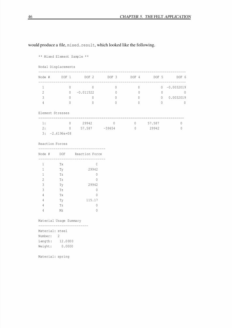
7/30/2019 Felt Manual
http://slidepdf.com/reader/full/felt-manual 68/236
46 CHAPTER 5. THE FELT APPLICATION
would produce a file, mixed.result, which looked like the following.
** Mixed Element Sample **
Nodal Displacements
-----------------------------------------------------------------------------
Node # DOF 1 DOF 2 DOF 3 DOF 4 DOF 5 DOF 6
-----------------------------------------------------------------------------
1 0 0 0 0 0 -0.0032019
2 0 -0.011522 0 0 0 0
3 0 0 0 0 0 0.0032019
4 0 0 0 0 0 0
Element Stresses
----------------------------------------------------------------------------
1: 0 29942 0 0 57.587 0
2: 0 57.587 -59654 0 29942 0
3: -2.4196e+08
Reaction Forces
-----------------------------------
Node # DOF Reaction Force
-----------------------------------
1 Tx 0
1 Ty 29942
1 Tz 0
2 Tz 0
3 Ty 29942
3 Tz 0
4 Tx 0
4 Ty 115.17
4 Tz 0
4 Mz 0
Material Usage Summary
--------------------------
Material: steel
Number: 2
Length: 12.0000
Weight: 0.0000
Material: spring
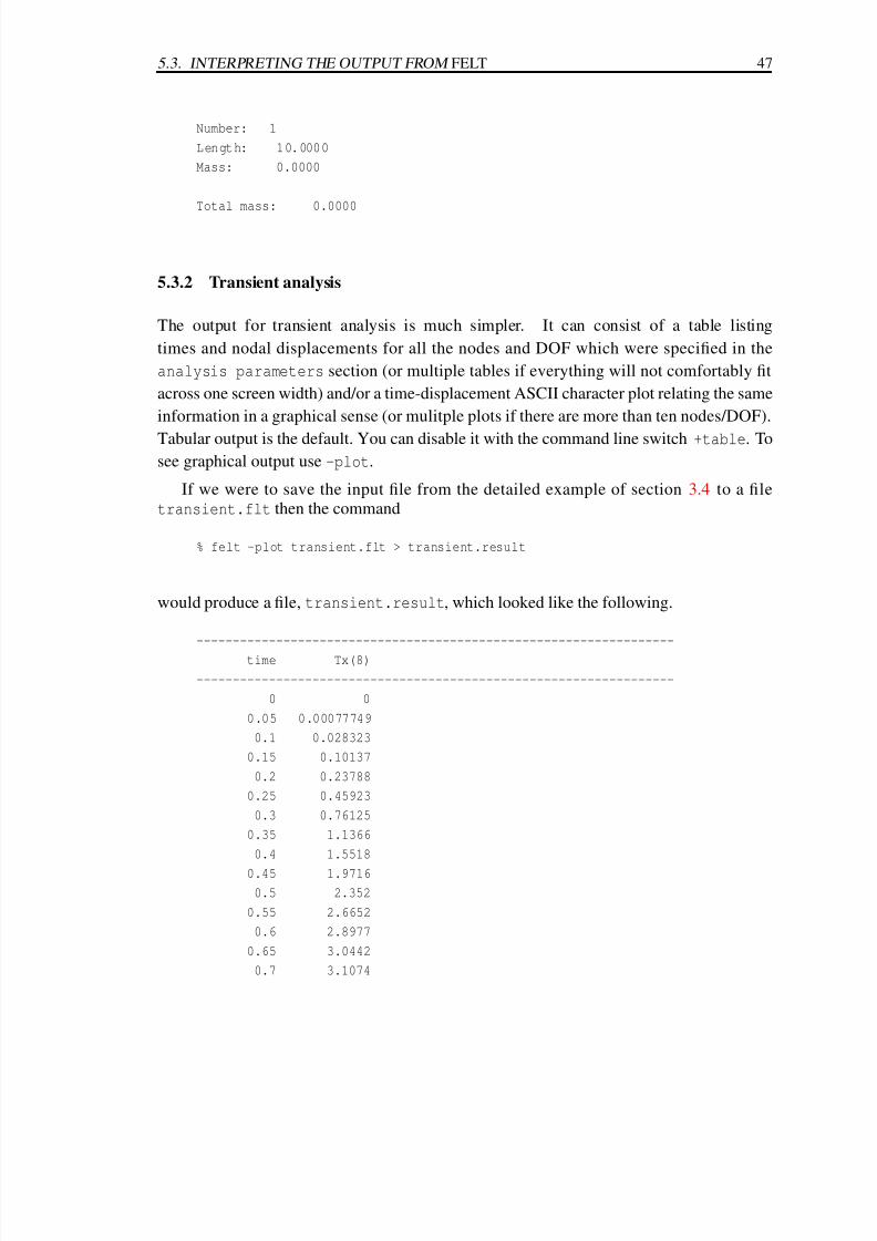
7/30/2019 Felt Manual
http://slidepdf.com/reader/full/felt-manual 69/236
5.3. INTERPRETING THE OUTPUT FROM FELT 47
Number: 1
Length: 10.0000
Mass: 0.0000
Total mass: 0.0000
5.3.2 Transient analysis
The output for transient analysis is much simpler. It can consist of a table listing
times and nodal displacements for all the nodes and DOF which were specified in the
analysis parameters section (or multiple tables if everything will not comfortably fit
across one screen width) and/or a time-displacement ASCII character plot relating the same
information in a graphical sense (or mulitple plots if there are more than ten nodes/DOF).
Tabular output is the default. You can disable it with the command line switch +table. To
see graphical output use -plot.
If we were to save the input file from the detailed example of section 3.4 to a file
transient.flt then the command
% felt -plot transient.flt > transient.result
would produce a file, transient.result, which looked like the following.
------------------------------------------------------------------
time Tx(8)
------------------------------------------------------------------
0 0
0.05 0.00077749
0.1 0.028323
0.15 0.10137
0.2 0.23788
0.25 0.45923
0.3 0.76125
0.35 1.1366
0.4 1.5518
0.45 1.9716
0.5 2.352
0.55 2.6652
0.6 2.8977
0.65 3.0442
0.7 3.1074
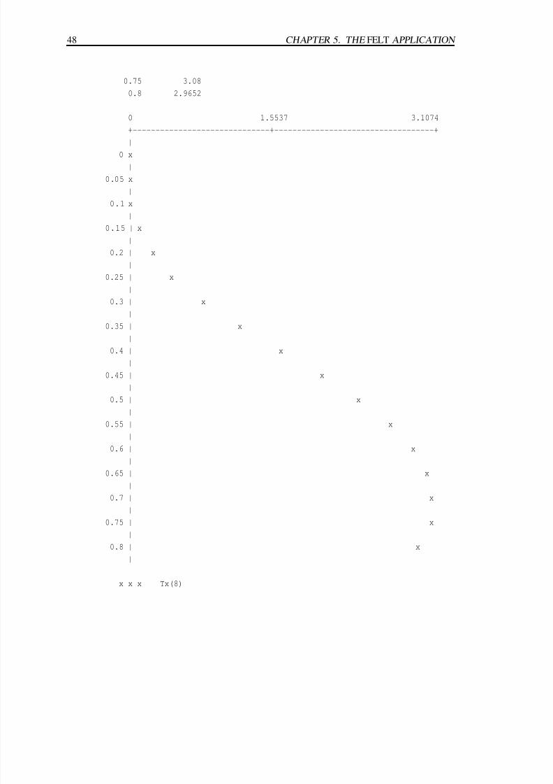
7/30/2019 Felt Manual
http://slidepdf.com/reader/full/felt-manual 70/236
48 CHAPTER 5. THE FELT APPLICATION
0.75 3.08
0.8 2.9652
0 1.5537 3.1074
+------------------------------+-----------------------------------+
|
0 x
|
0.05 x
|
0.1 x
|
0.15 | x
|
0.2 | x
|
0.25 | x
|
0.3 | x
|
0.35 | x
|
0.4 | x
|
0.45 | x
|
0.5 | x
|0.55 | x
|
0.6 | x
|
0.65 | x
|
0.7 | x
|
0.75 | x
|
0.8 | x|
x x x Tx(8)

7/30/2019 Felt Manual
http://slidepdf.com/reader/full/felt-manual 71/236
5.3. INTERPRETING THE OUTPUT FROM FELT 49
5.3.3 Modal analysis
The output from a modal analysis of a simple one story frame is shown below. Note that
the -matrices command-line switch was used to generate supplemental output (the ma-
trices prints before the results from the actual analysis) and that the -eigen switch was not
activated so full modal analysis was performed. The actual modal analysis results consist
of a listing of modal frequencies, a table of mode shape vectors (the eigenvectors)1, the
modal mass, damping, and stiffness matrices and the damping ratios in each mode.
M =
15.62 0 0 0 0 0
0 15.62 0 0 0 0
0 0 8.558e+04 0 0 0
0 0 0 15.62 0 0
0 0 0 0 15.62 0
0 0 0 0 0 8.558e+04
C =
194.8 0 720 -184.6 0 0
0 801.7 170.4 0 -1.049 170.4
720 170.4 1.123e+05 0 -170.4 1.846e+04
-184.6 0 0 194.8 0 720
0 -1.049 -170.4 0 801.7 -170.4
0 170.4 1.846e+04 720 -170.4 1.123e+05
K =
9.711e+04 0 3.6e+05 -9.231e+04 0 0
0 4.005e+05 8.521e+04 0 -524.4 8.521e+04
3.6e+05 8.521e+04 5.446e+07 0 -8.521e+04 9.231e+06
-9.231e+04 0 0 9.711e+04 0 3.6e+05
0 -524.4 -8.521e+04 0 4.005e+05 -8.521e+04
0 8.521e+04 9.231e+06 3.6e+05 -8.521e+04 5.446e+07
** Modal Analysis Example **
Modal frequencies (rad/sec)------------------------
Mode # Frequency
------------------------
1The current version of felt cannot generate a graphical representation of the mode shapes. See the dis-
cussion of mode shape plotting in chapter 8 for an example of how velvet can generate these kinds of plots.
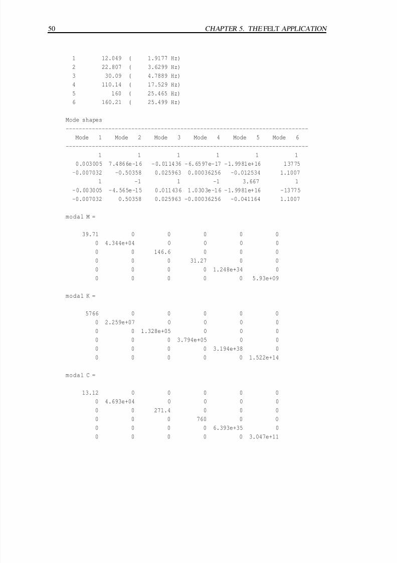
7/30/2019 Felt Manual
http://slidepdf.com/reader/full/felt-manual 72/236
50 CHAPTER 5. THE FELT APPLICATION
1 12.049 ( 1.9177 Hz)
2 22.807 ( 3.6299 Hz)
3 30.09 ( 4.7889 Hz)
4 110.14 ( 17.529 Hz)
5 160 ( 25.465 Hz)
6 160.21 ( 25.499 Hz)
Mode shapes
--------------------------------------------------------------------------
Mode 1 Mode 2 Mode 3 Mode 4 Mode 5 Mode 6
--------------------------------------------------------------------------
1 1 1 1 1 1
0.003005 7.4866e-16 -0.011436 -6.6597e-17 -1.9981e+16 13775
-0.007032 -0.50358 0.025963 0.00036256 -0.012534 1.1007
1 -1 1 -1 3.667 1
-0.003005 -4.565e-15 0.011436 1.0303e-16 -1.9981e+16 -13775
-0.007032 0.50358 0.025963 -0.00036256 -0.041164 1.1007
modal M =
39.71 0 0 0 0 0
0 4.344e+04 0 0 0 0
0 0 146.6 0 0 0
0 0 0 31.27 0 0
0 0 0 0 1.248e+34 0
0 0 0 0 0 5.93e+09
modal K =
5766 0 0 0 0 0
0 2.259e+07 0 0 0 0
0 0 1.328e+05 0 0 0
0 0 0 3.794e+05 0 0
0 0 0 0 3.194e+38 0
0 0 0 0 0 1.522e+14
modal C =
13.12 0 0 0 0 00 4.693e+04 0 0 0 0
0 0 271.4 0 0 0
0 0 0 760 0 0
0 0 0 0 6.393e+35 0
0 0 0 0 0 3.047e+11

7/30/2019 Felt Manual
http://slidepdf.com/reader/full/felt-manual 73/236
5.3. INTERPRETING THE OUTPUT FROM FELT 51
-------------------------
Modal damping ratios
-------------------------
1 0.01371
2 0.02368
3 0.03075
4 0.11032
5 0.16013
6 0.16034
5.3.4 Thermal analysis
The result from a static thermal analysis is a simple table showing the node number and
corresponding steady state temperature value; thermal stresses are not computed.
Output for transient thermal analysis can be tabular and/or graphical. The tabulated
results simply show the temperature as a function of time for whatever nodes were listed
in the nodes= specification of the analysis parameters (no dofs= specification is necessary
in transient thermal analysis). If you specify the -plot option on the command line then
felt will generate a simple ASCII plot of time versus temperature for these same nodes of
interest. Just as with transient structural analysis, tabular output can be turned off witht the
+table command-line switch.
5.3.5 Spectral analysis
Depending on how felt is invoked and the nature of the problem, the output for a spec-
tral analysis problem can either consist of transfer functions or of output spectra. If
the -transfer switch is given on the command line then all output will be for trans-
fer functions only. The transfer functions computed will be for all combinations of out-
put at the nodes and DOF defined by the nodes= and dofs= statements in the analysis
parameters section of the input file and input at all DOF with a force applied. For exam-
ple, if you define nodes 2 and 4 and DOF Tx and Ty as the relevant DOF in the analysis
parameters and there is force object with Fx and Fy non-zero applied to both nodes 3 and
7, then you will get sixteen transfer functions as results. If the input forcing is defined in
a spectral sense (e.g., with Sfx=) then you can also compute the output spectra at the out-
put DOF due to input at any forced DOF with spectral inputs. This is the default behavior
when the -transfer switch is not specified on the command-line. If none of the forces in a

7/30/2019 Felt Manual
http://slidepdf.com/reader/full/felt-manual 74/236
52 CHAPTER 5. THE FELT APPLICATION
problem have non-zero spectral input components then the only solution that is non-trivial
is with the -transfer switch invoked.
Just like for transient analysis, the output for spectral analysis (either transfer functions
or output spectra) can be tabular and/or plotted. ASCII plots of transfer functions or output
spectra (whichever are appropriate for the current problem) are generated if the -plot
switch is specified. Tabular output is generated by default and can be turned off with the
+table switch.

7/30/2019 Felt Manual
http://slidepdf.com/reader/full/felt-manual 75/236
Chapter 6
Using WinFElt
6.1 Introduction to WinFElt
The primary feature of the main WinFElt window is a standard text editor.
6.2 Solving a problem
Depending on what you want your solution to include, there are a couple of different ways
to go about solving a FElt problem from within WinFElt . In addition to the standard tabular
type FElt output you can also have WinFElt generate two-dimensional color shaded stress
or displacement plots and/or plots of the structure with magnified displacements applied.
For transient analysis problems graphical time-displacement or time-temperature plots are
available; in spectral analysis problems, plots of the transfer functions or ouput spectra are
available.
All of the WinFElt output windows have a File menu from which you can save or print
the results in that window. Line graphs are saved in Windows Metafile format (WMF) and
color contour plots are saved as Windows bitmaps (BMP) Text output can be saved as an
ASCII file. Once an output window is closed there is no way to bring the window back up
without resolving the problem.
One way to solve a problem is to select the solve option from the Solutions menu.
By default, this simply generates the standard FElt tabular output in a text output window
(figure 6.2). This window will contain either the mathematical solution of your problem or
the syntax errors encountered in solving the problem.
53

7/30/2019 Felt Manual
http://slidepdf.com/reader/full/felt-manual 76/236
54 CHAPTER 6. USING WINFELT
Figure 6.1: Main WinFElt editor with a sample problem.
Figure 6.2: The text output box.
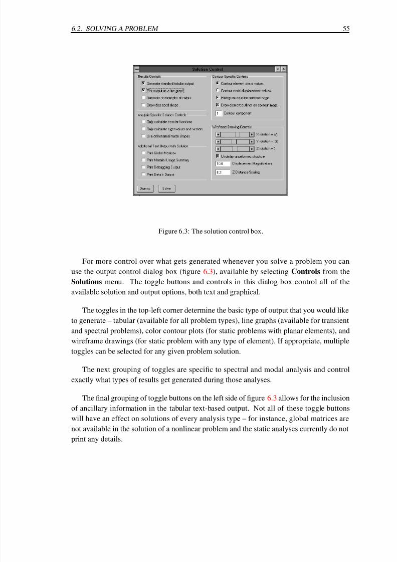
7/30/2019 Felt Manual
http://slidepdf.com/reader/full/felt-manual 77/236
6.2. SOLVING A PROBLEM 55
Figure 6.3: The solution control box.
For more control over what gets generated whenever you solve a problem you can
use the output control dialog box (figure 6.3), available by selecting Controls from the
Solutions menu. The toggle buttons and controls in this dialog box control all of the
available solution and output options, both text and graphical.
The toggles in the top-left corner determine the basic type of output that you would like
to generate – tabular (available for all problem types), line graphs (available for transient
and spectral problems), color contour plots (for static problems with planar elements), and
wireframe drawings (for static problem with any type of element). If appropriate, multiple
toggles can be selected for any given problem solution.
The next grouping of toggles are specific to spectral and modal analysis and control
exactly what types of results get generated during those analyses.
The final grouping of toggle buttons on the left side of figure 6.3 allows for the inclusion
of ancillary information in the tabular text-based output. Not all of these toggle buttons
will have an effect on solutions of every analysis type – for instance, global matrices are
not available in the solution of a nonlinear problem and the static analyses currently do not
print any details.
7/30/2019 Felt Manual
http://slidepdf.com/reader/full/felt-manual 78/236
56 CHAPTER 6. USING WINFELT
6.3 Text output
The text output from WinFElt is the most basic form of output that all applications in the
FElt system produce. That is, no matter how you specify and solve a FElt problem (either
with felt , velvet , or WinFElt ) the same kind of text output is available. Chapter 5 details the
interpretation of this basic output form.
6.4 Graphical output
6.4.1 Contour plots
The controls for color contour plots are available on the right side of the main controls dia-
log (6.3). The two radio buttons control whether element stress or nodal displacements are
used as the basis for the interpolation. For stress plots, the interpretation of the component
number is element specific and must be a valid index in the stress vector for each element
type in the problem. Consult Table 5.1 for details on what the stress vector consists of for
each element type. For displacement plots, the component is simply the displacement DOF
that you want to see plotted. In general, this should be one of the active global DOF for the
current problem.
Other contouring controls include toggles for histogram equalization and element
boundary overlay. Histogram equalization is a standard technique in image processing
for enhancing the contrast of images. If the overlay elements toggle is checked then the
outline of all the elements in the problem will be drawn in black on top of the color im-age. An example of stress contours (rendered here in greyscale) for the wrench example
supplied with WinFElt is shown in figure 6.4. Note that both histogram equalization and
element overlay were enabled for this plot.
6.4.2 Line graphs
6.4.3 Wireframe drawings
Most of the controls for wireframe drawing are specific to three-dimensional visualization.The three sliders control the rotation of the drawing about the three spatial axes. The
magnification determines the multiplicative factor by which nodal displacements will be
increased before the nodes are plotted. z scaling controls the front to back aspect ratio of
the resulting plot.

7/30/2019 Felt Manual
http://slidepdf.com/reader/full/felt-manual 79/236
6.4. GRAPHICAL OUTPUT 57
Figure 6.4: A color contour plot showing the principal stress component in a static problem usingconstant strain triangular elements
.
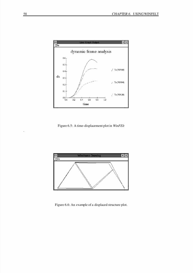
7/30/2019 Felt Manual
http://slidepdf.com/reader/full/felt-manual 80/236
58 CHAPTER 6. USING WINFELT
Figure 6.5: A time-displacement plot in WinFElt
.
Figure 6.6: An example of a displaced structure plot.

7/30/2019 Felt Manual
http://slidepdf.com/reader/full/felt-manual 81/236
6.4. GRAPHICAL OUTPUT 59
i

7/30/2019 Felt Manual
http://slidepdf.com/reader/full/felt-manual 82/236

7/30/2019 Felt Manual
http://slidepdf.com/reader/full/felt-manual 83/236
Chapter 7
The velvet Application
7.1 Introduction to the velvet GUI
velvet was designed as the primary user interface to the FElt system. Generally, if the FElt
system can solve a given problem, you will find it easier to specify, solve and analyze the
results for that problem right within the velvet GUI. velvet embodies all of the mathematical
features of FElt, as well as graphical pre- and post-processing and element generation.
The main velvet window consists of three major areas (Figure 7.1). The first is the list
of menu buttons down the left side of the window. This is the main control area for all of
the operations in velvet . The second is the command/status line across the bottom of the
window. This line is used to display messages and for keyboard based input. The third isthe drawing area, which occupies most of the window. This is the area in which you can
dynamically define and interact with the FElt problem.
The menus are used to define everything about a problem (nodes, elements, forces,
constraints, material properties, distributed loads), to configure velvet , to use the drawing
tools, to configure the drawing area and to save, open and solve problems.
7.2 General features of the interface
Many of the interface modules that you will see in velvet look very similar to one another.
Becoming familiar with a few basic operations that are common across all of these modules
will allow you to use velvet much more easily and flexibly.
In general, clicking an accept button will register the current state of a dialog with the
61
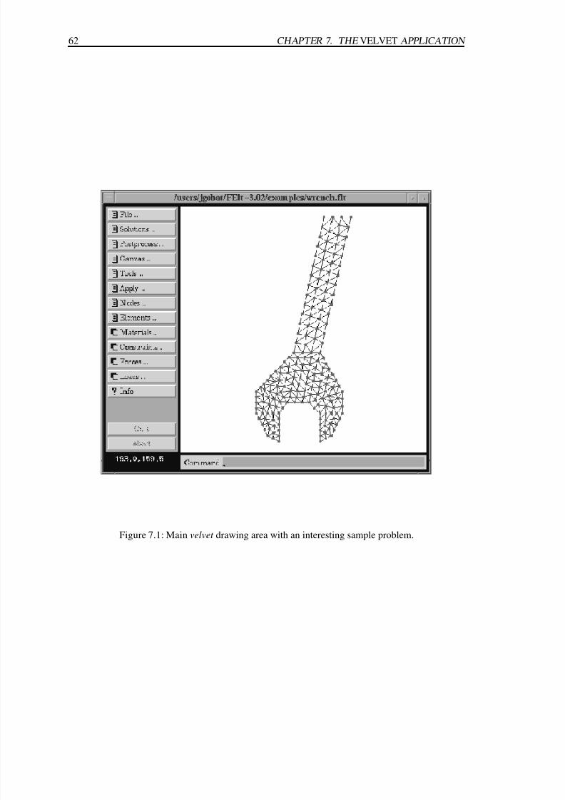
7/30/2019 Felt Manual
http://slidepdf.com/reader/full/felt-manual 84/236
62 CHAPTER 7. THE VELVET APPLICATION
Figure 7.1: Main velvet drawing area with an interesting sample problem.

7/30/2019 Felt Manual
http://slidepdf.com/reader/full/felt-manual 85/236
7.3. WORKING WITH FILES 63
rest of the application. Say you have a dialog with a few toggle buttons and a couple of
entry blanks. You could change the button states and type things into the entry blanks all
you wanted without actually affecting the rest of velvet . Once you click accept, however,
all of your changes become effective. This behavior is similar to an okay button in many
GUIs; the difference is that accept will not cause the dialog box to disappear. You willneed to click the dismiss button to do that.
Where there is a help button, you can click and hold it to view a brief help message
about that dialog. In some dialogs, additional help is available by clicking and holding
over special labels. This type of help will be discussed in more detail later.
A final factor that is common across GUI components is the idea of multiple mecha-
nisms. In general, there are three different ways that you can perform an action in velvet .
The first is by the standard point, click, and drag operations of the mouse. The second is
through keyboard shortcuts. The third is by entering commands or data into the command
window at the bottom of the main drawing area. For the most part, we will limit our initial
discussion to the mouse operations. Section 7.10 presents a summary of the equivalencies
between the different interface methods for those of you who want to become velvet power
users. For now, it should be enough to know that whenever velvet prompts you for a co-
ordinate you can either click in the drawing area or type in an x,y pair in the command
window (followed by a return of course). Similarly if you are being asked to select an
element or node; you can either type in the appropriate number or click on the appropriate
object.
7.3 Working with files
If you already have a FElt input file defined, the easiest way to start working with that
file is by specifying the filename on the shell command line when you invoke velvet . For
example,
% velvet foo.flt
Will start velvet and automatically load in the file foo.flt. The drawing area will be
initially configured to some reasonable values to allow you to view the entire problem. If
this file was saved from velvet then it will contain special sections that describe all of the
figures and the configuration of the drawing area when the file was saved. velvet will use
this information to reconstruct all of these things exactly as you left them.
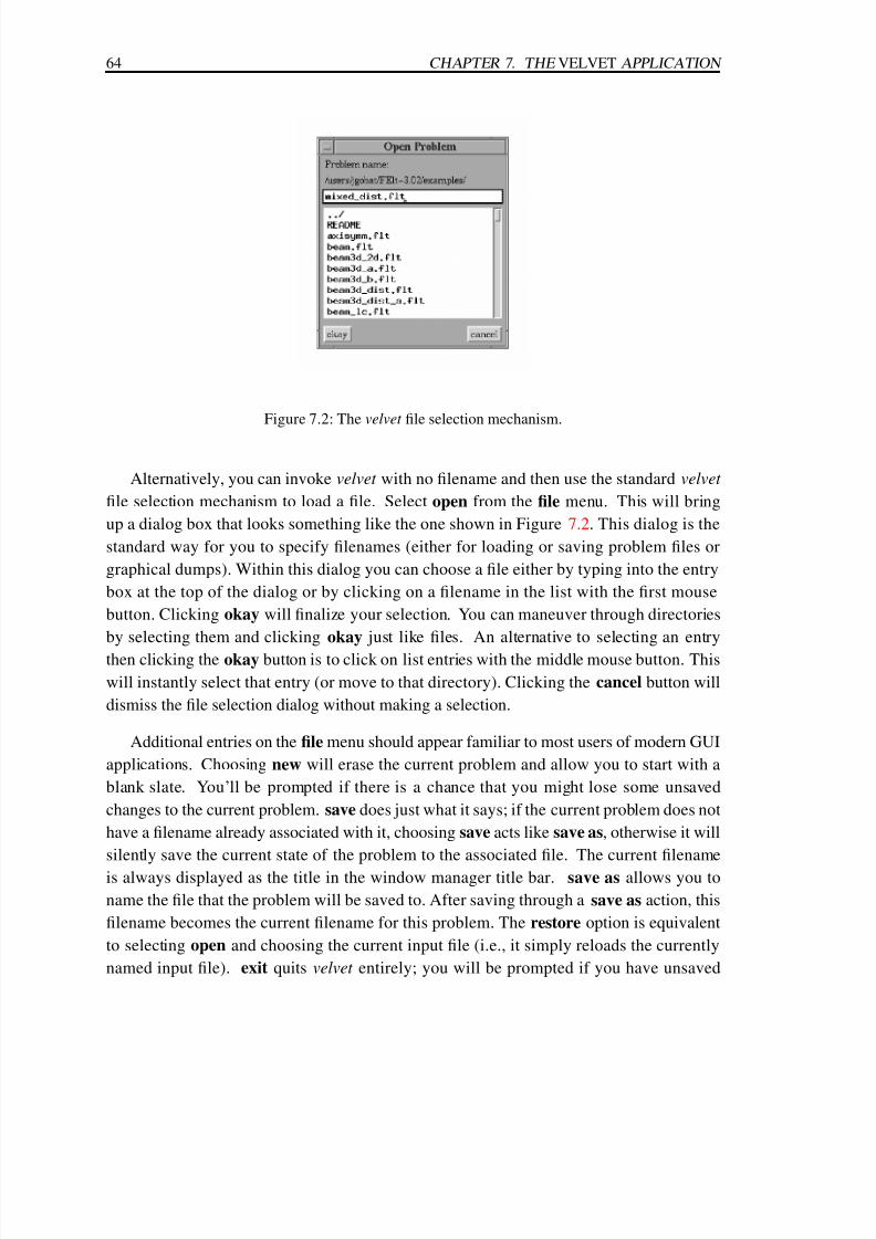
7/30/2019 Felt Manual
http://slidepdf.com/reader/full/felt-manual 86/236
64 CHAPTER 7. THE VELVET APPLICATION
Figure 7.2: The velvet file selection mechanism.
Alternatively, you can invoke velvet with no filename and then use the standard velvet
file selection mechanism to load a file. Select open from the file menu. This will bring
up a dialog box that looks something like the one shown in Figure 7.2. This dialog is the
standard way for you to specify filenames (either for loading or saving problem files or
graphical dumps). Within this dialog you can choose a file either by typing into the entry
box at the top of the dialog or by clicking on a filename in the list with the first mouse
button. Clicking okay will finalize your selection. You can maneuver through directories
by selecting them and clicking okay just like files. An alternative to selecting an entry
then clicking the okay button is to click on list entries with the middle mouse button. This
will instantly select that entry (or move to that directory). Clicking the cancel button will
dismiss the file selection dialog without making a selection.
Additional entries on the file menu should appear familiar to most users of modern GUI
applications. Choosing new will erase the current problem and allow you to start with a
blank slate. You’ll be prompted if there is a chance that you might lose some unsaved
changes to the current problem. save does just what it says; if the current problem does not
have a filename already associated with it, choosing save acts like save as, otherwise it will
silently save the current state of the problem to the associated file. The current filename
is always displayed as the title in the window manager title bar. save as allows you to
name the file that the problem will be saved to. After saving through a save as action, this
filename becomes the current filename for this problem. The restore option is equivalent
to selecting open and choosing the current input file (i.e., it simply reloads the currently
named input file). exit quits velvet entirely; you will be prompted if you have unsaved

7/30/2019 Felt Manual
http://slidepdf.com/reader/full/felt-manual 87/236
7.4. CONFIGURING THE DRAWING AREA 65
changes.
Note that when velvet saves a file, it will consist of the standard sections of a FElt file
plus special sections that describe the appearance of the drawing area. These ancillary
sections contain information that allows velvet to reconstruct the drawing area (including
tool figures, canvas configuration options and zoom state) when the corresponding FElt
file is loaded back into velvet . You should never have to worry about whether or not such
information exists. If a file with these sections is run through felt the information simply
will be ignored. If the information does not exist and you load the file into velvet then velvet
simply will make a best guess as to how to configure the main canvas area. The advantage
to having such a plain text description of the drawing area is that you can change this
information outside of velvet if you want to make quick changes to the problem appearance
but do not want to load velvet explicitly. Such an arrangement also allows you to easily
create defaults files which you can use to start-up velvet with your preferred configuration.
7.4 Configuring the drawing area
7.4.1 Basic controls
The primary means for setting up the drawing area is through the configure dialog under
the canvas menu (Figure 7.3). The left side of this dialog deals primarily with the minimum
and maximum coordinates of the drawing area, the snap size and the grid size. The right
side allows you to specify the colors and fonts to use for the different objects that appear
in the drawing area. The label font is used for node and element numbers. Also included
on the configure dialog are toggle buttons to control the status of snap, grid, element num-
bering and node numbering. Note that these four toggles are also available by selecting the
appropriate entry right on the canvas menu. You must click accept to make any of your
changes active.
As mentioned above, the snap and grid options act as toggle switches for these common
drawing aids. For those unfamiliar with these terms, grid produces a ruled grid across the
drawing area to help you locate yourself as you work and snap insures that mouse selected
coordinates will fall on regular fractions (i.e., a snap size of 0.25 insures that all of your
selections will be rounded to the nearest quarter unit). Note that the grid size (the spacing of
the rulings on the screen) and the snap size (the fraction to which your selected coordinates
will be automatically rounded) are controlled separately by entries in the configure dialog.
The node numbers option acts as a toggle switch for node numbering - in a crowded
problem, visible node numbers may not be helpful as they can tend to clutter the display.

7/30/2019 Felt Manual
http://slidepdf.com/reader/full/felt-manual 88/236
66 CHAPTER 7. THE VELVET APPLICATION
Figure 7.3: The configuration dialog box.
The same is true for the element numbers option. A check mark will appear next to themenu entry if the option is enabled.
7.4.2 Object coloring
Beyond the basic node color and element color controls provided in the canvas configura-
tion dialog (Figure 7.3), velvet also allows you to assign unique colors to individual forces,
constraints, material properties and distributed loads. Selecting color control from the
canvas menu will pop-up the colors dialog shown in Figure 7.4. The four smaller scrolled
lists on the left list all of the attributable objects (materials, distributed loads, constraints,
forces; see section 7.5) defined in the current problem. The larger list running down the
right side lists the available colors. By highlighting an entry in one of the four object lists
you can assign a color to that object.
In Figure 7.4, we see from the highlighted entries that the color for the material steel
is red. Any elements with material property steel will be rendered in red on the main
drawing canvas. If we wanted to change the color for steel to yellow, we could simply click
on yellow in the colors list. There is no accept button on this dialog; color assignments
take effect as soon as you select a color from the colors list. For any color changes to be
reflected in the drawing area, however, you need to click on recolor on the bottom of thecolor control dialog. Because recoloring the drawing area can be computationally intensive
it is a good idea to make all your color assignments first and then select recolor only once
when you are finished.
The precedence of coloring, from highest to lowest, is force, constraint, default for
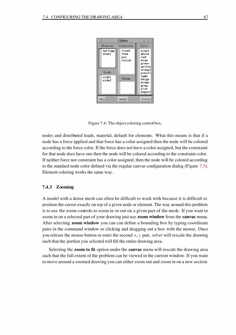
7/30/2019 Felt Manual
http://slidepdf.com/reader/full/felt-manual 89/236
7.4. CONFIGURING THE DRAWING AREA 67
Figure 7.4: The object coloring control box.
nodes and distributed loads, material, default for elements. What this means is that if a
node has a force applied and that force has a color assigned then the node will be colored
according to the force color. If the force does not have a color assigned, but the constraint
for that node does have one then the node will be colored according to the constraint color.
If neither force nor constraint has a color assigned, then the node will be colored according
to the standard node color defined via the regular canvas configuration dialog (Figure 7.3).
Element coloring works the same way.
7.4.3 Zooming
A model with a dense mesh can often be difficult to work with because it is difficult to
position the cursor exactly on top of a given node or element. The way around this problem
is to use the zoom controls to zoom in or out on a given part of the mesh. If you want to
zoom in on a selected part of your drawing just use zoom window from the canvas menu.
After selecting zoom window you can can define a bounding box by typing coordinate
pairs in the command window or clicking and dragging out a box with the mouse. Once
you release the mouse button or enter the second x,y pair, velvet will rescale the drawingsuch that the portion you selected will fill the entire drawing area.
Selecting the zoom to fit option under the canvas menu will rescale the drawing area
such that the full extent of the problem can be viewed in the current window. If you want
to move around a zoomed drawing you can either zoom out and zoom in on a new section

7/30/2019 Felt Manual
http://slidepdf.com/reader/full/felt-manual 90/236
68 CHAPTER 7. THE VELVET APPLICATION
(and repeat this as needed) or you can use the scroll bars on the left and bottom sides of the
drawing area to move around a zoomed canvas.
7.4.4 Dumping the drawing area
Use the save canvas option under the canvas menu when you want to save a “snapshot”
of the drawing area. Note that this will not be a dump of the entire velvet window as was
shown in Figure 7.1. The drawing area only will be saved either as an XWD or a standard
PostScript file. (Figure 7.11 illustrating the types of drawing tools available in velvet was
dumped with the save canvas option.) You select the filename through the standard file
dialog. Extra toggle buttons near the bottom of the dialog control whether the saved file
will be in XWD or PostScript format. This file could then be rendered for a presentationor for inclusion in a report. Additional drawing tools (see section 7.7) are available which
allow you to put a title, annotation or additional graphic objects in the drawing area in
addition to the standard presentation of nodes and elements. Note that because of the nature
of XWD’s, you need to make sure that no window is covering any part of the drawing area
whenever you do a dump in XWD format. This includes the file selection dialog; make
sure you move it out of the way before you click okay.
7.5 Drawing and defining a problem
Starting with a blank slate (either by invoking velvet without an input file or selecting new
from the file menu) you need to do several things to completely define a new problem. Say
for instance that you want to define the four node, three element, beam and truss exam-
ple problem considered earlier (Section 3.3, Figure 3.3). This problem uses two different
distributed loads, four different constraints, two element types and two materials. All of
these things need to be defined in order to properly solve the problem. The material prop-
erties must be defined before elements are added because an element must have a material
assigned to it. Likewise, at least one of the constraints must be defined before nodes can
be added because nodes must have a constraint assigned. In general, the procedure is to
setup whatever objects the problem might require (loads, forces, materials, constraints) be-
fore adding nodes and elements (generally nodes come first, since elements have to attach
between them).

7/30/2019 Felt Manual
http://slidepdf.com/reader/full/felt-manual 91/236
7.5. DRAWING AND DEFINING A PROBLEM 69
7.5.1 Defining attributable objects
The way that you work with these attributable objects (forces, loads, materials, constraints)
is by setting one of each as the active object of that type. This is particularly important
for materials and constraints. When you add a node it will automatically be assigned the
active constraint and when you add an element it will automatically be assigned the active
material. If you want to set the load on an element or the force on a node, or change the
constraint on a node or material on an element, you can use the apply menu. For instance,
choosing loads from this menu will allow you to apply the currently active distributed load
on an element of your choosing. To apply an object simply choose the appropriate entry
and then click on the nodes or elements which you wish to apply it to. velvet will keep
prompting you for additional objects until you click on quit or abort. If you wish to apply
an object to a group of nodes or elements (say for instance you wanted to apply a self-
weight load to all elements in the problem) you could simply drag out a bounding box by
clicking and holding the second mouse button. If you are applying forces or constraints,
every node in this box will be assigned the active object of that type. If you are applying
materials or loads, every element completely within the box will be assigned the active
object.
You set the active object of a given type by selecting it in the appropriate dialog box.
These dialogs can be popped-up by clicking on the materials, forces, loads or constraints
buttons in the main velvet control area. A picture of the constraint dialog after defining all
the constraints in our sample problem is shown in Figure 7.5. Several of the features that
you see here are exactly the same in the other three dialogs. Each has a name field and a
list of all the defined objects of that type. The six buttons (help, accept, dismiss, delete,
new, copy) across the bottom are also present in all four dialogs. The main area to the right
of the list and name is used for object specific definition.
Selecting an entry in the list will display the definition for that object and it will instantly
make that object the active definition for that kind of object. It would remain active even if
you were to dismiss the dialog box. You can use the name field to either set the name when
you are defining a new object or to rename an already defined object. For example, if you
bring up the material dialog in a brand new problem, you will be faced with a completely
blank slate. You can name your first material aluminum, define some material properties
and click accept. This would register aluminum as an available material and set it as the
currently active material. Now you want to define another material property, say springy.
You have two options. Clicking new will clear out all of the property fields and the name
field and you can name the new material springy and define its properties. Alternatively,
you can click copy and only the name field will be cleared. This is simply a convenient way

7/30/2019 Felt Manual
http://slidepdf.com/reader/full/felt-manual 92/236
70 CHAPTER 7. THE VELVET APPLICATION
Figure 7.5: The constraint dialog box.
to define a new material with properties similar to the previous material. All you have to
enter are a new name and any changed or additional material properties. In either case, you
need to click accept to register springy as a new material. If you still want aluminum as
the active material, you simply have to select aluminum in the list after you have accepted
springy. Finally, if you really meant to refer to aluminum by the name steel, you can
simply change the name in the field above the list and click accept. It is important tonote that the basic behavior of these buttons is exactly the same in all four dialogs. Only
the object specific information (discussed in more detail below) in the right side of each
behaves differently.
To delete an object you can simply click delete in the appropriate dialog box. Note
that velvet will not let you delete an object that is currently assigned to an element or node.
Clicking and holding the help button will display a brief help message for the given dialog
box.
The advantage to this mode of working with objects is that these dialogs can be left up
throughout your work session. You can have them up and easily change the active object
for a given type. There is no need to be constantly popping things up, selecting something
or changing something and then popping it down again only to need it again in 30 seconds.
If you’re sure you won’t be needing them after some initial setup, you can safely dismiss
them if you don’t like too much screen clutter.

7/30/2019 Felt Manual
http://slidepdf.com/reader/full/felt-manual 93/236
7.5. DRAWING AND DEFINING A PROBLEM 71
Figure 7.6: The material dialog box.
7.5.1.1 The material dialog
The object specific information for a material property is simply entered through the labeled
text boxes to the right of the material list (Figure 7.6). Additional help regarding each
property, including a list of which elements require that property to be defined, can be
gotten by clicking on the label for the given property (i.e., click on E for a description of
Young’s modulus). If a field is left blank, that property will be taken as 0.0.
7.5.1.2 The constraint dialog
The six toggle buttons shown in Figure 7.5 allow you to specify which DOFs are con-
strained by a boundary condition. If a toggle button is engaged, the corresponding text
field will also be used in constructing the boundary condition definition. If a button is en-
gaged and the text field is blank, that DOF will be fixed; if a button is engaged and that
field contains the word hinged then that DOF will be treated as a hinge (remember, hinged
DOFs only make sense on certain element types); if a button is engaged and the text field
contains a number, then that DOF will be defined as a displacement boundary condition; if
a button is engaged and the corresponding text field has a time-dependent expression then
that DOF will be treated as time-varying BC. Finally, if a button is not engaged, then thatDOF will remain completely unconstrained.
Initial conditions for transient analysis problems are defined with the initial displace-
ment, velocity, and acceleration entries. For initial displacement and velocity conditions
empty entries are taken as 0.0. For initial acceleration conditions, empty entries are un-

7/30/2019 Felt Manual
http://slidepdf.com/reader/full/felt-manual 94/236
72 CHAPTER 7. THE VELVET APPLICATION
Figure 7.7: The force dialog box.
defined. The distinction is that if all of the initial accelerations are undefined then the
mathematical engine will solve for an initial acceleration vector based on the initial dis-placement and velocity vectors. If any of the initial accelerations are specified in a problem
then any others which were left undefined will be taken as 0.0 and the mathematical engine
will use this vector as the initial acceleration.
7.5.1.3 The force dialog
The two toggle buttons at the top of the dialog toggle the display of force information
between the time domain forces (Fx ...Mz in a FElt file) and frequency domain spectral
inputs (Sfx ...Smz in a FElt file). Forces and moments (or spectra of forces and moments)in each of the three directions can be entered in the appropriate text field. If an entry is left
blank that component of the force will be taken as 0.0. The dialog pictured in Figure 7.7 is
from a model of a bicycle in which there are two static forces defined. Just like in a FElt
file, forces can be a time- or frequency-dependent function using the independent variables
t and w.
7.5.1.4 The load dialog
Figure 7.8 shows what the load dialog box looks like after we have defined both of the
distributed loads used in our sample problem. The eight toggle buttons define the direction
of the load. Note that these toggles function as a radio group, i.e., only one of them can
be selected at any one time. The text fields allow you to enter node, magnitude pairs much
the same way that you would define a load in a standard FElt input file. Remember that the
node specification refers to the local element number (i.e., 1 or 2 for a beam, 1, 2 or 3 for a
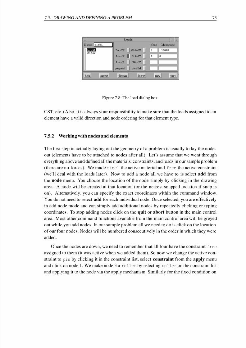
7/30/2019 Felt Manual
http://slidepdf.com/reader/full/felt-manual 95/236
7.5. DRAWING AND DEFINING A PROBLEM 73
Figure 7.8: The load dialog box.
CST, etc.) Also, it is always your responsibility to make sure that the loads assigned to an
element have a valid direction and node ordering for that element type.
7.5.2 Working with nodes and elements
The first step in actually laying out the geometry of a problem is usually to lay the nodes
out (elements have to be attached to nodes after all). Let’s assume that we went through
everything above and defined all the materials, constraints, and loads in our sample problem
(there are no forces). We made steel the active material and free the active constraint
(we’ll deal with the loads later). Now to add a node all we have to is select add from
the node menu. You choose the location of the node simply by clicking in the drawing
area. A node will be created at that location (or the nearest snapped location if snap is
on). Alternatively, you can specify the exact coordinates within the command window.
You do not need to select add for each individual node. Once selected, you are effectively
in add node mode and can simply add additional nodes by repeatedly clicking or typing
coordinates. To stop adding nodes click on the quit or abort button in the main control
area. Most other command functions available from the main control area will be greyed
out while you add nodes. In our sample problem all we need to do is click on the location
of our four nodes. Nodes will be numbered consecutively in the order in which they were
added.
Once the nodes are down, we need to remember that all four have the constraint free
assigned to them (it was active when we added them). So now we change the active con-
straint to pin by clicking it in the constraint list, select constraint from the apply menu
and click on node 1. We make node 3 a roller by selecting roller on the constraint list
and applying it to the node via the apply mechanism. Similarly for the fixed condition on

7/30/2019 Felt Manual
http://slidepdf.com/reader/full/felt-manual 96/236
74 CHAPTER 7. THE VELVET APPLICATION
node 4. We could have gotten around this by simply changing the active constraint before
we added each node. All we would have needed to do was leave the constraint dialog up
and click on the appropriate entry in the constraint list before we added the node that used
that constraint.
Before we can add the elements, we need to know how to set the element type. Like an
active object, we have to set a current element type before we can actually add any elements.
There is a distinction, however, as we cannot go back and apply a different element type
to an element. The only way to change the type of a given element is to delete it and add
a new element. We set the current element by choosing set type from the elements menu.
This will bring up a dialog similar to the standard file selection mechanism. Like the object
dialogs, the element selection dialog can be left up throughout your work session. The
current element type can be set simply by clicking on the appropriate name in the list. The
accept button is simply there in case you want to type in the element name. Typing beam3d
in the text field and clicking accept is equivalent to simply clicking on the beam3d entry inthe list.
Given this mechanism, the logical way to add the elements in our sample problem is
to set the current element type to beam and add elements 1 and 2. Elements are added by
selecting add from the elements menu and then clicking on nodes in the appropriate order,
or entering node numbers in the command window. velvet will wait until you have selected
the appropriate number of nodes for the current type of element before it prompts you to
add the next element. Click quit to stop adding elements. Click abort if you goofed up
on an element and just want to start over for that element (e.g., if you entered the first two
nodes wrong on a CST element).Once elements 1 and 2 are added we can change the element type to truss and add
element 3 by clicking on nodes 2 and 4. Before we did this we would probably also change
the active material to springy (or we could just change it with material from the apply
menu later).
We also still need to apply the distributed loads. All we have to do is set side1 active
by clicking it in the load dialog and apply it to element 1 from the apply menu. Then we
do the same thing for side2 and element 2.
Deleting nodes and elements (via delete under the appropriate menu) must proceed in
reverse order of adding nodes and elements. That is, a node can not be deleted if an element
is still attached to it, so the element must be deleted first. Elements can be deleted freely.
Deleting multiple nodes and elements is accomplished by clicking on one after the other
(quit or abort will finish deleting) or by clicking and holding the middle mouse button and
dragging out a box containing the nodes or elements to be deleted. As in deleting one at a

7/30/2019 Felt Manual
http://slidepdf.com/reader/full/felt-manual 97/236
7.6. MORE ON NODES AND ELEMENTS 75
Figure 7.9: The node information and editing dialog.
time, none of the selected nodes which are still attached to elements will be deleted.
7.6 More on nodes and elements
7.6.1 Editing nodes
In addition to simply adding and deleting nodes, velvet provides a powerful mechanism for
displaying and editing all of the information about a node. The node dialog box is shown
in Figure 7.9. You can raise this dialog either by selecting edit from the node menu or
by clicking directly on the node which you want to edit with the left mouse button. You
may want to use the former option (even though it seems a bit clumsier) in cases where
you can’t quite click on the right node. If you proceed from the menu option, you will
be prompted to either select the node with the mouse or to type the node number into the
command window. Once the dialog is up you can change the displayed node either with
the arrow keys in the dialog box, by clicking on a different node in the drawing area or
by selecting a new node through the edit option under the node menu. As a third option
for editing nodes you can click on a node with the third mouse button – this will raise the
node editing dialog and the constraint and force (if appropriate) dialogs with the assigned
objects for the selected node already highlighted. This is an easy way to take a complete
look at a given node; remember, however, that any changes you make to the node’s objectswill also affect any other nodes that have that object assigned to them.
The information available in the node dialog are the exact nodal coordinates, all six
nodal displacements (valid only after a problem has been solved), the lumped mass for the
node, the name of the constraint applied to the node and the name of the force (if any)

7/30/2019 Felt Manual
http://slidepdf.com/reader/full/felt-manual 98/236
76 CHAPTER 7. THE VELVET APPLICATION
applied to the node. The location, lumped mass, constraint and force can be modified
simply by editing the information in this dialog box. To change the applied constraint, you
can enter a new name into the text field or you can click on the constraint label to pop-up
a menu that will let you choose from a list of the currently defined constraints. The same is
true for forces by clicking on the force label. Note that while you can change the appliedforce on a node via the force option under the apply menu, editing the information in this
dialog is the only way to completely remove the applied force on a node. Just like the
object dialogs you need to click accept to make your changes effective. The rest of the
buttons on the bottom of the node dialog also behave exactly the same as the buttons on the
object dialogs.
velvet provides two ways for you to change a node’s location. The first is by changing
the location fields in the node dialog. The second is by selecting move from the node
menu. You can then select the node that you want to move by clicking on it, move to the
new location and click again to put it back down. Alternatively, just like you can click the first mouse button on a node to edit, you can click on a node with the second mouse
button to pick it up, move to a new location and click again with the second mouse button
to put it back down. Note that because velvet is basically a package for working with two-
dimensional problems, you cannot change the z coordinate of a node in the coordinate entry
fields of the node dialog.
7.6.2 Automatic node renumbering
velvet gives you two ways to optimize the node numbering in terms of reducing the profile
of the global stiffness matrix. The first way is to select renumber perm from the nodes
menu. This will actually rearrange all of the node numbers in the current problem - per-
manently. Generally you would choose this option where the node numbering was not
particularly important to your own understanding of the problem. This might be the case
if the elements had been automatically generated. If, on the other hand, you have a paper
sketch of the problem which you used to setup the problem then you may not want to lose
that particular node numbering scheme.
In this latter case what you can do is toggle temporary renumbering by selecting renum-
ber temp from the nodes menu. This toggle is equivalent to the -renumber command lineswitch in the command line application felt . If this switch is on, the nodes will be renum-
bered internally during the computations, and then restored to their original numbers before
you actually see any output, i.e. the output will reflect the original numbering scheme.
Both renumbering methods have their advantages. The permanent scheme reduces over-
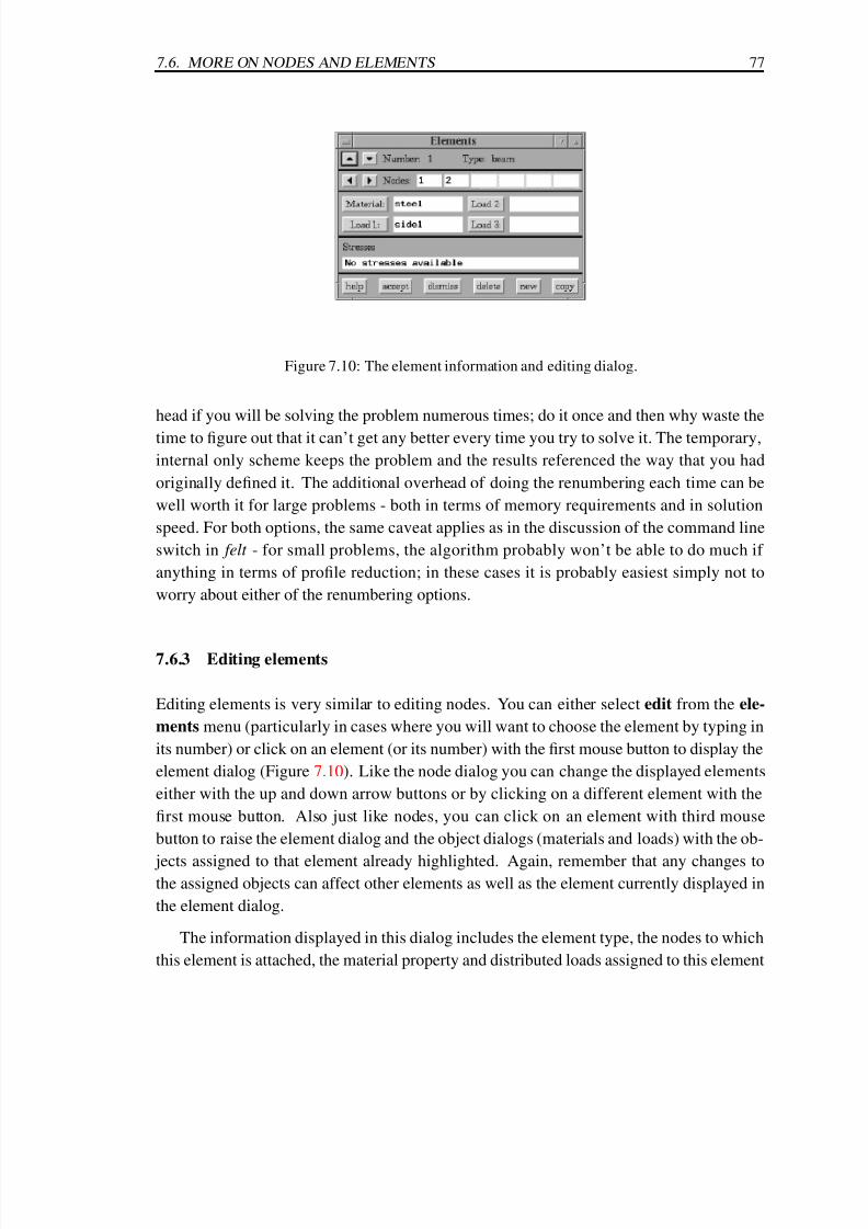
7/30/2019 Felt Manual
http://slidepdf.com/reader/full/felt-manual 99/236
7.6. MORE ON NODES AND ELEMENTS 77
Figure 7.10: The element information and editing dialog.
head if you will be solving the problem numerous times; do it once and then why waste the
time to figure out that it can’t get any better every time you try to solve it. The temporary,
internal only scheme keeps the problem and the results referenced the way that you had
originally defined it. The additional overhead of doing the renumbering each time can be
well worth it for large problems - both in terms of memory requirements and in solution
speed. For both options, the same caveat applies as in the discussion of the command line
switch in felt - for small problems, the algorithm probably won’t be able to do much if
anything in terms of profile reduction; in these cases it is probably easiest simply not to
worry about either of the renumbering options.
7.6.3 Editing elements
Editing elements is very similar to editing nodes. You can either select edit from the ele-
ments menu (particularly in cases where you will want to choose the element by typing in
its number) or click on an element (or its number) with the first mouse button to display the
element dialog (Figure 7.10). Like the node dialog you can change the displayed elements
either with the up and down arrow buttons or by clicking on a different element with the
first mouse button. Also just like nodes, you can click on an element with third mouse
button to raise the element dialog and the object dialogs (materials and loads) with the ob-
jects assigned to that element already highlighted. Again, remember that any changes tothe assigned objects can affect other elements as well as the element currently displayed in
the element dialog.
The information displayed in this dialog includes the element type, the nodes to which
this element is attached, the material property and distributed loads assigned to this element

7/30/2019 Felt Manual
http://slidepdf.com/reader/full/felt-manual 100/236
78 CHAPTER 7. THE VELVET APPLICATION
and, if the problem has been solved, the stress results for this element. If an element uses
more than six nodes, you can use the side to side arrow buttons next to the node list to scroll
through them. The dialog gives you a simple mechanism for changing the nodes, material
and loads for a given element. Editing the material and loads is just like the constraint
and force fields in the node dialogs. You can either type into the text field or click on theappropriate label and choose from a menu of currently available objects. Like forces in the
node dialog, changing the information in the element dialog is the only way to completely
remove all the loads from an element. Once again of course, you need to click accept to
make any changes effective. The other buttons across the bottom and their functions should
be very familiar to you by now.
7.7 Using tools
The drawing tools are intended to be aids for meshing up or annotating a problem. For
instance, you can draw a circle by selecting circle from the tools menu and then place
nodes along the circle. The actual figure on the screen does not affect the solution of the
problem in any way. velvet will prompt you in the command window for the necessary
coordinates for each figure type. As usual, you can choose coordinates either with the
mouse or by typing in the command window. In general, however, you must enter all of
the coordinate locations for a given figure with the same input method; what this means is
that if you enter the coordinates of the first point of a line with the keyboard then you will
have to enter the second point with keyboard input as well or, alternatively, if you select
the center of a circle with the mouse then you will have to select the radius with the mouse
as well.
Titles and comments can be entered in the drawing area by selecting text from the tools
menu option. As mentioned earlier, the drawing area could then be dumped to an XWD and
the result could serve as documentation or a figure in a presentation, complete with color
annotation. Figure 7.11 shows such a dump with examples of the available tools. Tool
color and font is controlled from the configure option under the canvas menu. In addition
to text and circles, the velvet drawing toolbox currently includes lines, arcs, polylines, and
rectangles.
To draw a line with the mouse you have to click at the start point and hold the mouse
button while you drag the line to the end point. Rectangles work the same way; click and
hold while you drag out a box. For circles your mouse click will select a center point, and
as you move the mouse while still holding the button, your circle will expand about that
center. When drawing polylines with the mouse, use the first mouse button to select the

7/30/2019 Felt Manual
http://slidepdf.com/reader/full/felt-manual 101/236
7.7. USING TOOLS 79
Figure 7.11: Examples of all the tools available in velvet .
7/30/2019 Felt Manual
http://slidepdf.com/reader/full/felt-manual 102/236
80 CHAPTER 7. THE VELVET APPLICATION
starting point by a simple click (not a click and hold). Additional end points are defined by
additional clicks of the first mouse button. You can stop adding endpoints by clicking the
third mouse button. If you want a closed polyline, you can simply click the second mouse
button and velvet will draw a line from your current position to the starting point of the
polyline.
Tools can be deleted from the screen just like nodes and elements, either one at a time or
with a window. Once in delete mode (select delete from the tools menu), individual figures
can be selected by clicking with the left mouse button or a window can be drawn with the
middle mouse button. The delete operation proceeds until quit or abort is clicked. Moving
a tool figure that already is drawn on the screen is also straightforward; simply select move
from the tools menu, click on the figure that you want to move and then click again once
you have dragged it to its new location.
The ancillary sections in the FElt file that are created when you save a problem from
velvet record all your tool figures. If these sections are available when you reload a problem,
the tools will automatically be redrawn for you.
7.8 Material databases and defaults files
Often, you will find that certain objects or material properties are being used over and
over again in different problems. Dummy FElt files can be used to make easy use of this
repetitive information. Starting velvet with a FElt file that contains a couple of common
constraint definitions means that those definitions will not need to be specified explicitly
within velvet - they will be there for use on start-up. Similarly for other types of objects.
Note that loading a defaults file from within velvet is just like opening a new input file,
everything in the current problem will be lost. You can use the canvas configuration
and display list sections of a FElt file to create a custom canvas configuration in a
defaults file.
Material databases are also special cases of FElt input files. They are given special
treatment within velvet because they are so convenient. Whole classes of material types
and shapes (W-shape beams, standard diameter bars, etc.) can be stored in a material
database and loaded into velvet at any time with the open database command under the
file menu. Any changes to material properties or additions of new materials can be saved
simply by selecting update database from the file menu. The current set of materials is
the only thing that is retained when a new input file is loaded or a new problem is started
within velvet .
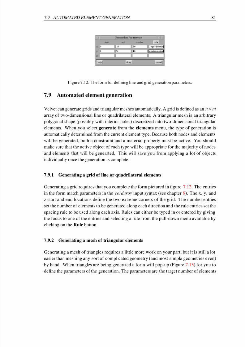
7/30/2019 Felt Manual
http://slidepdf.com/reader/full/felt-manual 103/236
7.9. AUTOMATED ELEMENT GENERATION 81
Figure 7.12: The form for defining line and grid generation parameters.
7.9 Automated element generation
Velvet can generate grids and triangular meshes automatically. A grid is defined as an n×m
array of two-dimensional line or quadrilateral elements. A triangular mesh is an arbitrary
polygonal shape (possibly with interior holes) discretized into two-dimensional triangularelements. When you select generate from the elements menu, the type of generation is
automatically determined from the current element type. Because both nodes and elements
will be generated, both a constraint and a material property must be active. You should
make sure that the active object of each type will be appropriate for the majority of nodes
and elements that will be generated. This will save you from applying a lot of objects
individually once the generation is complete.
7.9.1 Generating a grid of line or quadrilateral elements
Generating a grid requires that you complete the form pictured in figure 7.12. The entries
in the form match parameters in the corduroy input syntax (see chapter 9). The x, y, and
z start and end locations define the two extreme corners of the grid. The number entries
set the number of elements to be generated along each direction and the rule entries set the
spacing rule to be used along each axis. Rules can either be typed in or entered by giving
the focus to one of the entries and selecting a rule from the pull-down menu available by
clicking on the Rule button.
7.9.2 Generating a mesh of triangular elements
Generating a mesh of triangles requires a little more work on your part, but it is still a lot
easier than meshing any sort of complicated geometry (and most simple geometries even)
by hand. When triangles are being generated a form will pop-up (Figure 7.13) for you to
define the parameters of the generation. The parameters are the target number of elements

7/30/2019 Felt Manual
http://slidepdf.com/reader/full/felt-manual 104/236
82 CHAPTER 7. THE VELVET APPLICATION
Figure 7.13: The form for defining triangle generation parameters.
that you want to generate, the α area constraint factor and the number of holes in your
generation region. The area constraint factor is defined as
Aelt ≤ α Aregion
target, (7.1)
where Aregion is the total area of the generation region and Aelt is the maximum area of a
generated element.
Once the parameters are defined, click okay to begin defining the boundaries of your
problem. Regions are defined by putting down marker points in the drawing area (they must
be put down in a counter-clockwise order). To finish the boundary, click on the quit button.
If the number of holes was greater than zero then each hole must be defined just like the
boundary was defined – by laying down a series of marker points – but in clockwise order.
Each hole is finished by clicking the quit button. The generation process can be aborted
by clicking the abort button. Typing shift-bkspc will delete the last marker point that was
laid down, thus allowing you to correct mistakes without restarting the entire sequence.
Once all the regions are defined, velvet will automatically begin generating the mesh.
7.10 Keyboard interface mechanisms
7.10.1 Keyboard shortcuts
As in most graphical environments, the pointer can only do so much for you; often it will
be easier for you to use the keyboard. True, you could get away with using the mouse for
everything, but in the long run you will work more efficiently if you learn the keyboard
interface mechanisms.
There are two basic ways that you can use key presses in place of mouse clicks. The
first are commonly called keyboard shortcuts. This means that rather than selecting solve
from the problem menu, you can simply press ctrl-v . A complete list of these shortcuts is
given in the quick reference table at the end of this section.

7/30/2019 Felt Manual
http://slidepdf.com/reader/full/felt-manual 105/236
7.10. KEYBOARD INTERFACE MECHANISMS 83
The second common way to use the keyboard is to move through groups of buttons
and text fields with tab to change the input focus and use space to activate the button
or change the toggle state. This is a very convenient way of working with dialog boxes
like the object dialogs (forces, materials, constraints, loads), the file selection dialog, the
node and element dialogs, the configure dialog, the triangular mesh parameter dialog andthe solution dialog. When one of the dialogs has the window manager focus there are a few
special keyboard shortcuts that you can use as well. ctrl-h is equivalent to help, return
is accept or okay, esc is dismiss or cancel, ctrl-d is delete, ctrl-n is new, and ctrl-c is
copy.
7.10.2 Command names
All of the commands that are available through menu options in the main control area
are also available by typing a text command into the command window at the bottom of
the main window. To use a text command simply type it into the command window and
hit return . If you just type return with no command entered, velvet will repeat the last
command that you entered. The following table lists the equivalencies for each command.
The first column lists the name of the menu button in the control area, the second lists
the applicable entry under that menu, if any, and the third lists the command name(s) that
perform the same action. The fourth column provides additional ways that you can perform
the same function, either through a keyboard shortcut or through mouse interaction with
the drawing area.

7/30/2019 Felt Manual
http://slidepdf.com/reader/full/felt-manual 106/236
84 CHAPTER 7. THE VELVET APPLICATION
Menu Command Text command Other alternatives
File New new Ctrl-f n
Open open Ctrl-f o
Save save Ctrl-f s
Save as save as Ctrl-f w
Restore restore Ctrl-f rOpen database open database
Update database update database
Exit exit Ctrl-f x
Solutions Solve solve Ctrl-v
Animate animate
Results/Output define output
Problem/Analysis define problem
Postprocess Plot stresses plot stresses
Plot displacements plot displacements
Plot structure plot structure
Contouring contour
Wireframe wireframe
Canvas Configure configure
Color control colorsZoom to fit zoom all Ctrl-Z
Zoom window zoom Ctrl-z
Save canvas dump
Snap snap Ctrl-s
Grid grid Ctrl-g
node numbering node numbers Ctrl-n
element numbering element numbers Ctrl-e
Apply Materials apply material Ctrl-a m
Forces apply force Ctrl-a f
Constraints appply constraint Ctrl-a c
Loads apply load Ctrl-a l
Tools Circle draw circle Ctrl-t c
Arc draw arc Ctrl-t a
Rectangle draw rectangle Ctrl-t rPolygon draw polygon Ctrl-t p
Line draw line Ctrl-t l
Text draw text Ctrl-t t
Delete delete tool
Move move tool
Nodes Add add node
Edit edit node button 1 on node
Delete delete node
Move move node button 2 on node
Lumped mass lumped mass
Renumber perm renumber nodes
Renumber temp toggle renumber
Elements Add add element
Editedit element
button 1 on elementSet type set element
Generate generate
Materials edit material Ctrl-d m
Constraints edit constraint Ctrl-d c
Forces edit force Ctrl-d f
Loads edit load Ctrl-d l
Quit Esc or button 3
Abort Ctrl-c
7/30/2019 Felt Manual
http://slidepdf.com/reader/full/felt-manual 107/236
7.11. COMMAND LINE OPTIONS 85
7.11 Command line options
Some of the above functionality can be enabled, disabled or altered via command line
switches when you invoke velvet . In addition to the standard X toolkit options (-display,
etc.) you can use any of the following to control the behavior and set the start-up condi-
tion of velvet . Each of these options can also be set through your Xresources using the
associated resource name.
-sensitive Enable sensitive/insensitive menu switching. velvet has two major modes
of operation, normal mode and edit mode. Each mode allows only certain
operations to be performed. This option allows disabling of the menus con-
trolling the inactive operations. This is the default behavior but may be
inappropriate on a slow server. Associated resource: *sensitiveMenus.
+sensitive Disable sensitive/insensitive menu switching. Associated resource:
*sensitiveMenus.
-numbers Enable element and node numbering on start-up. This is the default behav-
ior. Associated resource: *numbers.
+numbers Disable the drawing of element and node numbering on start-up. On some
servers the node and element numbers may take some extra time to draw
on big problems and since you’ll probably turn them off anyways to reduce
clutter, you can use this switch to disable them from the start. Associate
resource: *numbers.
-nodeColor color
Sets the color of nodes and node numbers. The default color is blue. Asso-
ciated resource: *nodeColor.
-elementColor color
Sets the color of elements and element numbers. The default color is black.
Associated resource: *elementColor.
-toolColor colorSets the color of tools (rectangles, lines, circles) and interactive windows.
The default color is red. Associated resource: *toolColor.
-labelFont font
Sets the font used for node and element numbers. The default font is 5x8.

7/30/2019 Felt Manual
http://slidepdf.com/reader/full/felt-manual 108/236
86 CHAPTER 7. THE VELVET APPLICATION
Associated resource: *labelFont.
-toolFont font
Sets the font used for text drawn using the tools. The default font is fg-22.
Associated resource: *toolFont.
-cpp filename
substitute filename for the pre-processor to run on the input file.
-nocpp do not run the input file through the pre-processor.
-Idirectory
add directory to the standard search path for include files in the pre-
processor.
-Uname undefine the macro name in the pre-processor.
-Dname=value
define name to be the macro value in the pre-processor.
7/30/2019 Felt Manual
http://slidepdf.com/reader/full/felt-manual 109/236
Chapter 8
Post-processing with velvet
8.1 Solving a problem with velvet
Depending on what you want your solution to include, there are a couple of different ways
to go about solving a FElt problem from within velvet . In addition to the standard tabu-
lar type FElt output (see section 5.3) you can also have velvet generate two-dimensional
color shaded stress or displacement plots and/or plots of the structure with magnified dis-
placements applied. For transient analysis problems graphical time-displacement or time-
temperature plots replace the ASCII versions that felt produces. Transient structural analy-
sis can also include an animation of the simulation. For spectral analysis, graphical plots of
the transfer functions or ouput spectra replace felt ’s ASCII versions. velvet can also drawgraphical representations of mode shapes for modal analysis problems.
One way to solve a problem is to select the solve option from the solutions menu. By
default, this simply generates the standard FElt output. This window will contain either
the mathematical solution of your problem or the syntax errors encountered in solving the
problem.
For more control over what gets generated whenever you solve a problem you can use
the output control dialog box (Figure 8.1, available by selecting results/output from the
solutions menu. The toggle buttons in this dialog box control all of the available solution
and output options, both text and graphical.
The three toggles at the top–left of the dialog mimick three of the switches available
in felt ; they control the computations that are performed for modal or spectral analysis.
The felt output toggle controls whether or not you want to see any of the standard textual
output that felt would generate. If the felt output toggle is on then the other three textual
87

7/30/2019 Felt Manual
http://slidepdf.com/reader/full/felt-manual 110/236
88 CHAPTER 8. POST-PROCESSING WITH VELVET
Figure 8.1: The output control dialog box.
output toggles mimick command-line switches that are available in felt (see chapter 5) to
control the printing of additional information within the textual output.
For graphical output, the toggles for stress, structure and displacement plots simply
allow you to automatically invoke these post-processing options (see below) on solution.
The other two options (time-displacement plots and mode shape plots) are only available
during a problem solution (i.e., only by selecting the appropriate toggle in this dialog and
then solving the problem). The line plot option generates a graphical line plot (as opposed
to the ASCII plot that you would get with felt output) for transient or spectral results. A
graphical time-displacement plot is shown in Figure 8.2. Figure 8.3 is an example of a
mode shape plot. Note that velvet only draws a single mode at a time and that the regu-
lar problem geometry is drawn as an underlying dotted line; you can cycle forward and
backward through the individual modes using the < and > buttons.
Given the settings in our example control box, the output for a static model of a bicycle
would be the two windows shown in Figures 8.4 and 8.5. (The input file for this problem
can be found as bicycle boys.flt in the tests directory of the standard FElt distributions.)
You can save any of the velvet output by clicking save at the bottom of the output
window. A file dialog will pop-up and allow you to name the file which you wish to save
to. Depending on the type of output, you may have the option of saving in one of several
different file formats. Time-displacement, wireframe structure, and mode shape plots can
be saved in either XWD or PostScript format. Text output can be saved as an ASCII file.
Color contours of stress and displacement can be saved in PPM or encapsulated PostScript
(EPS) format.
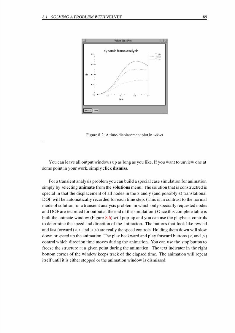
7/30/2019 Felt Manual
http://slidepdf.com/reader/full/felt-manual 111/236
8.1. SOLVING A PROBLEM WITH VELVET 89
Figure 8.2: A time-displacement plot in velvet
.
You can leave all output windows up as long as you like. If you want to unview one at
some point in your work, simply click dismiss.
For a transient analysis problem you can build a special case simulation for animation
simply by selecting animate from the solutions menu. The solution that is constructred is
special in that the displacement of all nodes in the x and y (and possibly z) translational
DOF will be automatically recorded for each time step. (This is in contrast to the normal
mode of solution for a transient analysis problem in which only specially requested nodes
and DOF are recorded for output at the end of the simulation.) Once this complete table is
built the animate window (Figure 8.6) will pop-up and you can use the playback controls
to determine the speed and direction of the animation. The buttons that look like rewind
and fast forward (<< and >>) are really the speed controls. Holding them down will slow
down or speed up the animation. The play backward and play forward buttons (< and >)
control which direction time moves during the animation. You can use the stop button to
freeze the structure at a given point during the animation. The text indicator in the right
bottom corner of the window keeps track of the elapsed time. The animation will repeat
itself until it is either stopped or the animation window is dismissed.
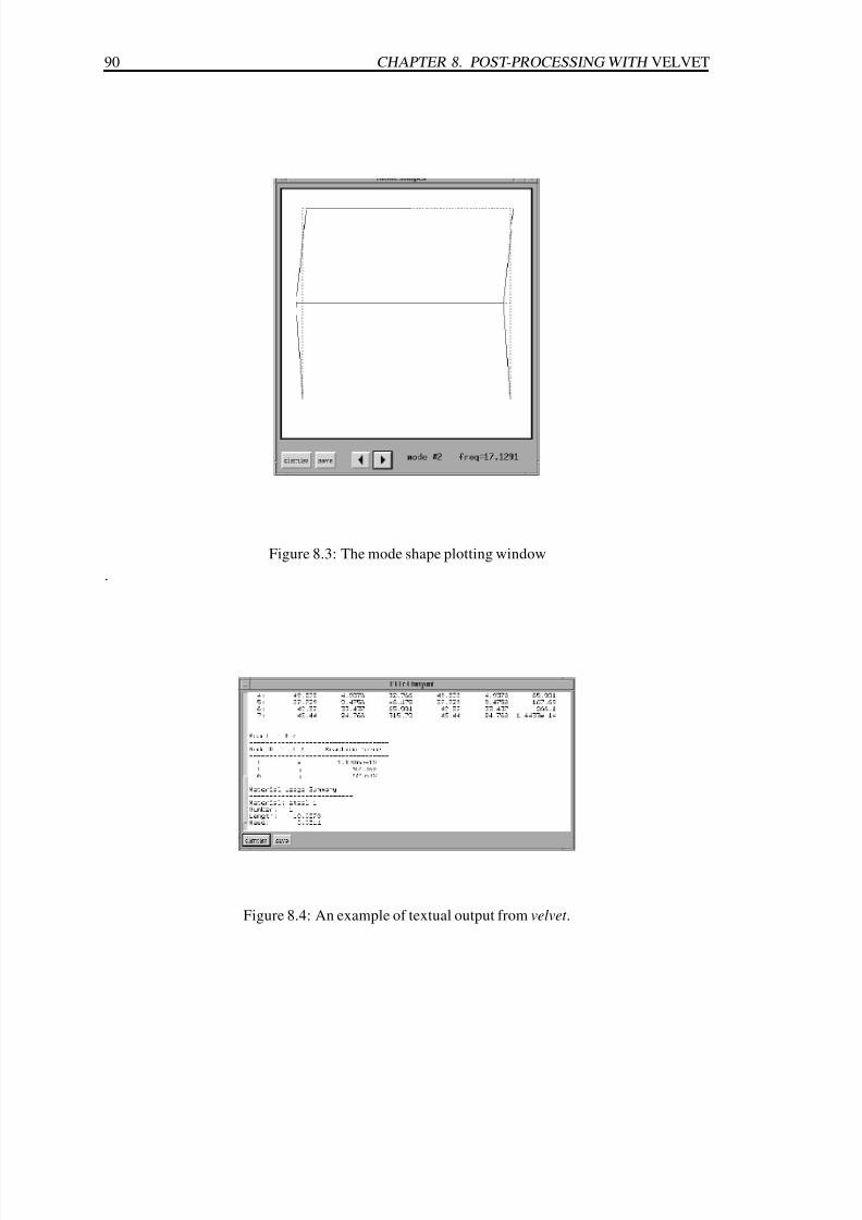
7/30/2019 Felt Manual
http://slidepdf.com/reader/full/felt-manual 112/236
90 CHAPTER 8. POST-PROCESSING WITH VELVET
Figure 8.3: The mode shape plotting window
.
Figure 8.4: An example of textual output from velvet .

7/30/2019 Felt Manual
http://slidepdf.com/reader/full/felt-manual 113/236
8.1. SOLVING A PROBLEM WITH VELVET 91
Figure 8.5: An example of a displaced structure plot.
Figure 8.6: An animation in velvet
.

7/30/2019 Felt Manual
http://slidepdf.com/reader/full/felt-manual 114/236
92 CHAPTER 8. POST-PROCESSING WITH VELVET
8.2 Problem description and analysis parameters
The problem description and analysis parameters section of a regular FElt input
file are mimicked in velvet by the problem and analysis dialog box (Figure 8.7). This dialog
is available by selecting problem/analysis from the solutions menu. The problem title text
entry defines the header that will be used for textual output and on graphical line plots. The
analysis mode is defined by engaging one of the toggle buttons just below the problem title
at the top of the dialog. The mass-mode toggles below the analysis toggles allow you to
select either consistent or lumped mass formulations for element mass matrices.
For a transient structural and thermal analysis problems, there are several parameters
which control the numerical integration in time. The text entries down the left side of the
dialog allow you to fill in values for these parameters in the γ , β, and α text entries. For
both transient and spectral analysis the range of time or frequency over which to perform
the computations is defined by the start , stop, and step text entries. Note that the valuefor start is ignored in transient analysis types. Values for the global Rayleigh damping
proportionality constants are defined with the Rk and Rm text entries. Remember that if
either of these values is non-zero then the Rayleigh damping for this problem will be based
on these values and the global stiffness and mass matrices as opposed to elemental material
values of Rk and Rm and the element stiffness and mass matrices.
The DOF toggles and the node entries allow you to define the list of nodes and which
DOF at each of those nodes that you would like to have included in the output when the
problem is solved. Click on the left and right arrow keys to scroll through the complete list
of nodes if you are interested in more than six of them.The push buttons on the bottom of the dialog box are standard of course. The solve
and animate buttons are simply there as a convenience; pushing either button will cause
the current state of the dialog to be registered (as if you had pushed accept) and then the
appropriate action to be taken just as if you had selected solve or animate from the main
solutions menu.
8.3 Controlling the post-processing
8.3.1 Controlling contour plots
The controls for color contour plots are available by selecting contouring from the post-
processing menu. On the dialog (Figure 8.8), there are identical controls for stress and
displacement plots. On the stress side, the component specifies which stress component
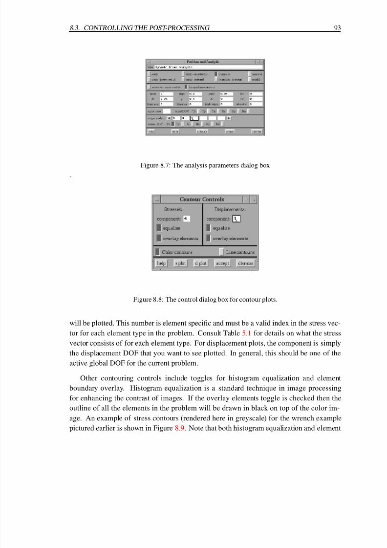
7/30/2019 Felt Manual
http://slidepdf.com/reader/full/felt-manual 115/236
8.3. CONTROLLING THE POST-PROCESSING 93
Figure 8.7: The analysis parameters dialog box
.
Figure 8.8: The control dialog box for contour plots.
will be plotted. This number is element specific and must be a valid index in the stress vec-
tor for each element type in the problem. Consult Table 5.1 for details on what the stress
vector consists of for each element type. For displacement plots, the component is simply
the displacement DOF that you want to see plotted. In general, this should be one of the
active global DOF for the current problem.
Other contouring controls include toggles for histogram equalization and element
boundary overlay. Histogram equalization is a standard technique in image processing
for enhancing the contrast of images. If the overlay elements toggle is checked then the
outline of all the elements in the problem will be drawn in black on top of the color im-
age. An example of stress contours (rendered here in greyscale) for the wrench example
pictured earlier is shown in Figure 8.9. Note that both histogram equalization and element

7/30/2019 Felt Manual
http://slidepdf.com/reader/full/felt-manual 116/236
94 CHAPTER 8. POST-PROCESSING WITH VELVET
overlay were enabled for this plot.
In addition to the standard buttons for help, accept, and dismiss, you can use the s plot
and d plot buttons as an alias for selecting either plot stresses or plot displacements from
the main postprocessing menu item. Both buttons cause the dialog state to be accepted
before the plot is generated.
8.3.2 Controlling structure plots
Additional control over structure plots is available through the wireframe dialog box (Fig-
ure 8.10). The majority of these controls are specific to three-dimensional visualization.
The three dial widgets control the rotation of the drawing about the three spatial axes. The
magnification determines the multiplicative factor by which nodal displacements will be
increased before the nodes are plotted. z scaling controls the front to back aspect ratio
of the resulting plot. The toggle for hidden line removal is non-functional in the currentversion of velvet . The defaults reflected in the dialog pictured in Figure 8.10 were used to
generate our earlier example of the structural plot of the bicycle (Figure 8.5).
The extra button at the bottom of the dialog plot is equivalent to pressing accept and
selecting plot structure from the postprocessing menu.
8.3.3 Controlling animation
The analysis parameters used in constructing a displacement table for an animation are
the same as those that would be used in a normal solution for that problem in transient
analysis mode, except for the nodes and DOF. As mentioned above, an animation will
automatically solve for all nodes at the x and y (and z if the problem is 3d) translational
DOF. The magnification of the displacements during the animation can be controlled via
the same magnification control that is used in structure plots. Likewise for 3-d animations,
the 3-d drawing parameters will be taken from the controls in the wireframe control dialog
box.

7/30/2019 Felt Manual
http://slidepdf.com/reader/full/felt-manual 117/236
8.3. CONTROLLING THE POST-PROCESSING 95

7/30/2019 Felt Manual
http://slidepdf.com/reader/full/felt-manual 118/236
96 CHAPTER 8. POST-PROCESSING WITH VELVET
Figure 8.10: The wireframe plotting control dialog box.

7/30/2019 Felt Manual
http://slidepdf.com/reader/full/felt-manual 119/236
Chapter 9
The corduroy Application
9.1 Introduction
corduroy is a command line application for automatically generating nodes and elements. It
takes a text input file and generates FElt format nodes and elements for inclusion into a FElt
problem. Like felt then, it is a command line interface to some of the same functionality
that you can get in velvet . However, unlike felt and velvet , which share their file syntax (the
standard FElt syntax), corduroy has its own special syntax to describe the way elements are
generated.
9.2 The corduroy syntax
9.2.1 Specifying basic parameters
corduroy allows you to generate elements in five different ways – along a single line, as
a three-dimensional grid of line elements, as a two-dimensional grid of four-node planar
elements, as a three-dimensional grid of solid elements and as a two-dimensional mesh
of triangular elements. Each type of generation is described in its own section; there can
be multiple types and multiple sections of a given type in any given file. Besides these
descriptive sections there are only a few basic parameters, all of which are optional. Order
of specifications does not matter in a corduroy file except for numbering of generated nodes
and elements and the end statement which must always come at the end of a file (and is
not optional). As in regular FElt files, comments can be denoted with /* and */ as in the C
programming language and symbolic expressions may be substituted for any non-integer
value.
97

7/30/2019 Felt Manual
http://slidepdf.com/reader/full/felt-manual 120/236
98 CHAPTER 9. THE CORDUROY APPLICATION
You can use start-node= and start-element= to specify the number for the first
things that get generated. Normally, corduroy starts the numbering at one and then numbers
sequentially as it moves from section to section of your input file. These two specifications
allow you to override these starting points in situations where you may already have a few
elements and nodes defined and you are going to attach the things that get generated aftercorduroy has done its work.
constraint= and material= will assign a constraint or material name to the initial
node and element. This is simply a convenience; you will need to be sure to go back and
actually define these objects after everything is generated and you are putting the finishing
touches on the problem definition.
9.2.2 Generating elements along a line
The simplest case of element generation is a line which is divided up into an arbitrarynumber of elements. You might use something like this if you were examining the accuracy
of a cantilever beam model and wanted to use successively higher numbers of elements
from one case to the next. The corduroy specification for a line section looks like this
line
element-type = beam
start = (0,0,0)
end = (5,5,5)
number = 20
This example would generate twenty beam elements all lying along the line from the origin
to a point at x=5, y=5, z=5 in rectangular Cartesian coordinates. The default element type
for both line and grid generation is truss. Valid type names are the same as in a standard
FElt file (see chapter 3).
9.2.3 Generating a grid of line elements
Another relatively simple case is when you want to generate a three-dimensional grid of
line elements. An excellent example of when this might be useful is for a model of a steel
frame structure. The specification for a grid is
grid
element-type = beam
start = (0,0,0) end = (100,500,100)
x-number = 4 y-number = 20 z-number = 4
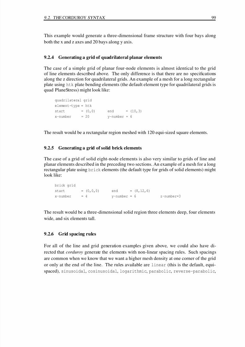
7/30/2019 Felt Manual
http://slidepdf.com/reader/full/felt-manual 121/236
9.2. THE CORDUROY SYNTAX 99
This example would generate a three-dimensional frame structure with four bays along
both the x and z axes and 20 bays along y axis.
9.2.4 Generating a grid of quadrilateral planar elements
The case of a simple grid of planar four-node elements is almost identical to the grid
of line elements described above. The only difference is that there are no specifications
along the z direction for quadrilateral grids. An example of a mesh for a long rectangular
plate using htk plate bending elements (the default element type for quadrilateral grids is
quad PlaneStress) might look like:
quadrilateral grid
element-type = htk
start = (0,0) end = (10,3)
x-number = 20 y-number = 6
The result would be a rectangular region meshed with 120 equi-sized square elements.
9.2.5 Generating a grid of solid brick elements
The case of a grid of solid eight-node elements is also very similar to grids of line and
planar elements described in the preceding two sections. An example of a mesh for a long
rectangular plate using brick elements (the default type for grids of solid elements) might
look like:
brick grid
start = (0,0,0) end = (8,12,6)
x-number = 4 y-number = 6 z-number=3
The result would be a three-dimensional solid region three elements deep, four elements
wide, and six elements tall.
9.2.6 Grid spacing rules
For all of the line and grid generation examples given above, we could also have di-
rected that corduroy generate the elements with non-linear spacing rules. Such spacings
are common when we know that we want a higher mesh density at one corner of the grid
or only at the end of the line. The rules available are linear (this is the default, equi-
spaced), sinusoidal, cosinusoidal, logarithmic, parabolic, reverse-parabolic,
7/30/2019 Felt Manual
http://slidepdf.com/reader/full/felt-manual 122/236
100 CHAPTER 9. THE CORDUROY APPLICATION
and reverser-logarithmic. If we are placing the sides of n elements along a line, then
we need to locate n + 1 nodes on the line. The coordinate xi of each node is defined as
follows for each of the spacing rules
linear : xi = Lβ (9.1)cosinusoidal : xi = L − L cos
π2β
(9.2)
sinusoidal : xi = L sinπ
2β
(9.3)
logarithmic : xi = L log10 (1 + 9β) (9.4)
parabolic : xi = Lβ2 (9.5)
reverse− logarithmic : xi = L − L log10 (10 − 9β) (9.6)
reverse−parabolic : xi = L β (9.7)
(9.8)
where β = (i − 1)/n.
9.2.7 Generating a triangular mesh
The triangular mesh generation capabilities of corduroy use Jonathan Shewchuk’s Triangle
routine. In addition to specifications that describe the boundary and the holes of your two-
dimensional region, you must also define the approximate number of elements to generate
and a constraint on the maximum area of any one generated element. The number of
elements is specified with target=. The area constraint is given using alpha=, where α is
defined such that
Aelt ≤ α Atotal
total. (9.9)
The entire corduroy input file to generate the nodes and elements for the wrench model
pictured in Figure 7.1 would look like this.
start-node = 1 /* unnecessary as this is the default */
start-element = 1
triangular mesh
element-type = CSTPlaneStress
angtol = 20 dmin = 0.5 min = 100 /* except for min and max */
angspc = 30 kappa = 0.25 max = 300 /* these are defaults */
boundary = [
(0,50)
(20,10)

7/30/2019 Felt Manual
http://slidepdf.com/reader/full/felt-manual 123/236
9.2. THE CORDUROY SYNTAX 101
(40,0)
(40,50)
(55,70)
(95,70)
(115,50)
(115,0)
(135,10)
(155,50)
(155,90)
(115,160)
(170,404)
(122,404)
(67,160)
(0,90)
]
end
To generate a mesh in a rectangular plate with two side by side rectangular holes in it,
the input file could look like
triangular mesh /* use all defaults, including CSTPlaneStress */
boundary = [
(0,0)
(20,0)
(20,10)
(0,10)
]
hole = [
(6,3)
(8,3)
(8,7)
(6,7)
]
hole = [
(12,3)
(14,3)
(14,7)
(12,7)
]

7/30/2019 Felt Manual
http://slidepdf.com/reader/full/felt-manual 124/236
102 CHAPTER 9. THE CORDUROY APPLICATION
end
Note that the hole definitions do not need to come before the boundary, but that points must
always be specified in a counter-clockwise order.
9.3 Using corduroy
The only options to corduroy are the standard cpp options as in both felt and velvet (like
those two programs, corduroy runs all of its input through the pre-processor before actually
operating on it) and a -debug flag which causes corduroy to reproduce as output what it
thinks it received for input. To generate, all you need to do is create an input file with a text
editor and then run corduroy with the name of this file as the last argument on the command
line. Output will be directed to standard out. So if you had a generation description in a file
foo.crd, you could turn it into the basics of a FElt file called foo.flt with the following
command
% corduroy foo.crd > foo.flt
9.4 Incorporating output into a FElt file
Becausecorduroy
only generates the node and element sections of a FElt file, you still havesome editing to do before you can call the problem completely defined and actually try to
solve it with felt or velvet . In general, you will have to define forces and constraints to assign
to nodes and material properties (and possibly distributed loads) to assign to elements.
Remember, the material= and constraint= specification are only a convenience. These
two names will simply be assigned to the first element and node, respectively (and all the
following elements and nodes by default). You still need to actually define those objects
and assign any different objects to appropriate nodes and elements. To do all this defining
and assigning you can either use your favorite text editor or you can load the problem into
velvet and do it all from there.
One thing to keep in mind whenever you use corduroy to generate a problem for you
is that corduroy is not very good at node numbering. Using the renumbering features of
either felt or velvet is highly recommended with corduroy generated problems. In general
the problems that you will use corduroy for will be quite large and thus the reduction in
memory and solution time would be significant even if node numbering had been intelligent

7/30/2019 Felt Manual
http://slidepdf.com/reader/full/felt-manual 125/236
9.4. INCORPORATING OUTPUT INTO A FELT FILE 103
to start with; the reductions for large problem with initially very bad numbering can be
remarkable.

7/30/2019 Felt Manual
http://slidepdf.com/reader/full/felt-manual 126/236

7/30/2019 Felt Manual
http://slidepdf.com/reader/full/felt-manual 127/236
Chapter 10
The burlap Application
10.1 Introduction to the burlap environment
burlap is a mathematical environment designed for adding new element types to FElt and
extending the current set of finite element analyses. burlap can best be described as a
mathematical software package, similar to matlab or octave, but with the data structures
of FElt. It was designed as an alternative to trying to understand and modify the C code
of the FElt library, which was difficult for even us to do, much less engineers with little C
programming experience.
burlap has its own syntax for manipulating matrices, like that of matlab. However,
burlap also includes all of the FElt data types as well, such as nodes, elements, constraints,
etc., which eliminates the need for having large arrays of numbers, where the third number
is the material thickness and the fourth number is the cross-sectional area, etc.
Any analysis that can be performed with felt can be performed with burlap. Although
the burlap code is slower than the compiled C code of the FElt library, burlap’s interac-
tive environment makes prototyping new element types and new analyses much easier. At
present, however, there is no support for executing burlap code from velvet .
10.2 Using burlap
10.2.1 Interacting with burlap
The syntax of burlap is designed to be intuitive and is best illustrated by examples. A
detailed discussion of the syntax can be found in Chapter 11. The simplest way to start
105

7/30/2019 Felt Manual
http://slidepdf.com/reader/full/felt-manual 128/236
106 CHAPTER 10. THE BURLAP APPLICATION
burlap is to simply type burlap on the command line, or burlap foo.b if you wish to
execute the burlap file foo.b. You can also specify command line options that qualify what
you want to do.
-help | -h Display a brief help message which lists all of the available command line
options and then exits.
-quiet | -q
Do not print the start-up message regarding copyright information.
-alias | -a
Do not define the set of built-in aliases.
-interactive | -i
Enter interactive mode by reading expressions from the terminal after pro-cessing the input files. Normally, burlap will simply exit after processing
any input files.
-no-interactive | -n
Do not enter interactive mode. This flag tells burlap to simply exit if no files
are given. It is useful if you have burlap aliased to burlap -i and wish to
override the effect of the -i flag.
-source command-file | -s command-file
Read commands from command-file on start-up.
-felt felt-file | -f felt-file
Use felt-file to define the current FElt problem.
Since burlap can load and process a FElt file, it also accepts the standard -nocpp, -cpp,
-I, -U, and -D flags common to felt and velvet . If you simply type burlap, you will be
presented with some copyright information and a prompt.
This is burlap, copyright 1995 by Jason I. Gobat and Darren C. Atkinson.
This is free software, and you are welcome to redistribute it under certain
conditions, but there is absolutely no warranty. Type help ("copyright")
for details. Use the -q option to suppress this message.
[1] _
7/30/2019 Felt Manual
http://slidepdf.com/reader/full/felt-manual 129/236
10.2. USING BURLAP 107
If burlap was compiled with the GNU readline library, then you have complete
command-line editing and history, as in bash. (A complete discussion of the editing ca-
pabilities can be found in the documentation of the readline library.) At the prompt, you
can enter expressions to be evaluated.
[ 1 ] 1 + 2
[2] write (1 + 2)
3
[ 3 ] a = 1 + 2
[4] write (a)
3
[5] write ([1, 2, 3])
1 2 3
[6] write ([1; 2; 3])
1
2
3
[7] write ([1, 2, 3] + [4, 5, 6])
5 7 9
As illustrated above, write() is used to print results and = is the assignment operator.
Also notice from the first expression that burlap does not print the result of every expressionlike matlab does. But, just like matlab, matrices are delimited by square brackets with
elements separated by commas and rows separated by semicolons.
If you type alias you should see the following list. (If burlap is not compiled with the
readline library then the list will be slightly different.)
exit exit ( )
h history (20)
help help ("!$")
ls system ("ls !*")
quit exit ( )
burlap has a very simple syntax with all computations being done through either oper-
ators, such as +, or functions, such as write(). But, since exit() and help() are rather
non-intuitive, you can alias commands to be whatever you want, just like csh. So, you can
just type exit or quit to leave burlap. Typing help will present you with a list of all the
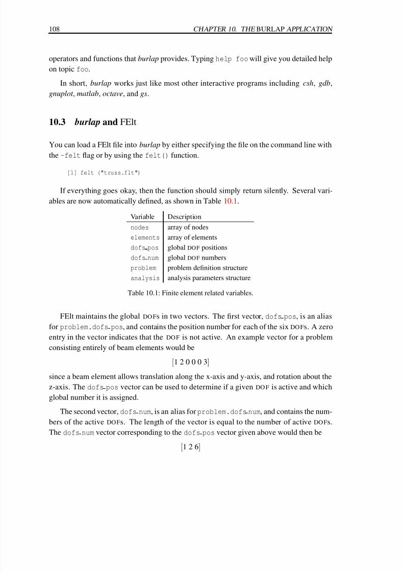
7/30/2019 Felt Manual
http://slidepdf.com/reader/full/felt-manual 130/236
108 CHAPTER 10. THE BURLAP APPLICATION
operators and functions that burlap provides. Typing help foo will give you detailed help
on topic foo.
In short, burlap works just like most other interactive programs including csh, gdb,
gnuplot , matlab, octave, and gs.
10.3 burlap and FElt
You can load a FElt file into burlap by either specifying the file on the command line with
the -felt flag or by using the felt() function.
[1] felt ("truss.flt")
If everything goes okay, then the function should simply return silently. Several vari-
ables are now automatically defined, as shown in Table 10.1.
Variable Description
nodes array of nodes
elements array of elements
dofs pos global DO F positions
dofs num global DO F numbers
problem problem definition structure
analysis analysis parameters structure
Table 10.1: Finite element related variables.
FElt maintains the global DO Fs in two vectors. The first vector, dofs pos, is an alias
for problem.dofs pos, and contains the position number for each of the six DO Fs. A zero
entry in the vector indicates that the DO F is not active. An example vector for a problem
consisting entirely of beam elements would be
[1 2 0 0 0 3]
since a beam element allows translation along the x-axis and y-axis, and rotation about the
z-axis. The dofs pos vector can be used to determine if a given DO F is active and which
global number it is assigned.The second vector, dofs num, is an alias for problem.dofs num, and contains the num-
bers of the active DO Fs. The length of the vector is equal to the number of active DO Fs.
The dofs num vector corresponding to the dofs pos vector given above would then be
[1 2 6]

7/30/2019 Felt Manual
http://slidepdf.com/reader/full/felt-manual 131/236
10.3. BURLAP AND FELT 109
since the first, second, and sixth DO Fs are active. burlap ensures that the two vectors are
always kept consistent.
All arrays start at one, so nodes (1) designates the first node in the problem, and
nodes (1).constraint designates the constraint associated with that node. A period (.)
is used to access a field of a FElt object. In general the field names are the same as the
names used in the FElt input file. For example, constraint is the field name for accessing
the constraint object assigned to a node with the constraint= syntax in the FElt file.
[2] write (nodes)
array of node
[3] write (elements)
array of element
[4] write (nodes (1))
node (1)
[5] write (nodes (1).constraint)constraint (free)
[6] write (elements (1).material.A)
0.0004
[7] m = elements (1).material
[8] write ("A = ", m.A, " E = ", m.E)
A = 0.0004 E = 2.1e+11
10.3.1 Element objects
Elements have the same field names as those used in the FElt file with additional fields forholding the computed matrices and stress values, as shown in Table 10.2. For example,
e.number will return the element number of the element e and e.material.t will return
the thickness of the element’s material; e.nodes (1) will return the first node of the ele-
ment and e.nodes (1).x will return the x-coordinate of that node. Note that loads and
distributed are synonymous, as are num loads and num distributed.
10.3.2 Node objects
Like elements, nodes have some fields that are defined through the FElt input file with addi-
tional fields to contain the result of computations, as shown in Table 10.3. As an example,
n.constraint will return the constraint assigned to the node n, and n.constraint.name
will return the name of that constraint; n.dx will return the displacement vector and n.dx
(1) will return the first component of that vector. Note that the displacement vector may
be accessed either as a vector by using dx, or as individual components, such as Tx. This

7/30/2019 Felt Manual
http://slidepdf.com/reader/full/felt-manual 132/236
110 CHAPTER 10. THE BURLAP APPLICATION
Field name Description
number element number
nodes array of nodes
K stiffness matrix
M mass matrixmaterial material object
definition element type definition
loads array of distributed loads
num loads number of loads
stresses array of element stresses
ninteg number of integration points
distributed array of distributed loads (loads)
num distributed number of distributed loads (num loads)
Table 10.2: Fields of an element object.
is simply a shorthand; assigning to an individual component is the same as assigning to the
result of indexing the displacement vector. The equivalent force vector, eq force, is used
in transforming distributed loads on an element into equivalent forces on its nodes.
10.3.3 Material objects
Materials have the fields named by the FElt input syntax, as shown in Table 10.4. Forexample, m.rho will return the density of the material m and m.A will return its cross-
sectional area.
10.3.4 Force objects
Force objects allow the forces and moments to be accessed as individual components or as a
vector, as shown in Table 10.5. For example, f.force will return the force vector of f and
f.force (4) will return the moment about the x axis, which is equivalent to f.force.Mx.
For transient problems, a force or moment may vary with time. In felt , this is described
by an expression in terms of t. A component of a force may be assigned a string value
which will be interpreted by burlap as an expression. Note that evaluating the compo-
nent will evaluate the expression at time t=0. There is currently no way to determine if a
component is assigned a time-varying expression.
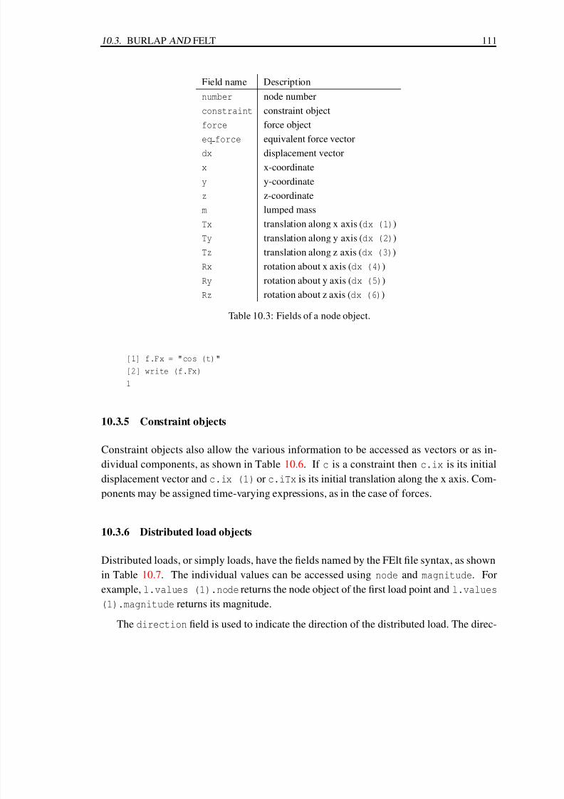
7/30/2019 Felt Manual
http://slidepdf.com/reader/full/felt-manual 133/236
10.3. BURLAP AND FELT 111
Field name Description
number node number
constraint constraint object
force force object
eq force equivalent force vectordx displacement vector
x x-coordinate
y y-coordinate
z z-coordinate
m lumped mass
Tx translation along x axis (dx (1))
Ty translation along y axis (dx (2))
Tz translation along z axis (dx (3))
Rx rotation about x axis (dx (4))
Ry rotation about y axis (dx (5))Rz rotation about z axis (dx (6))
Table 10.3: Fields of a node object.
[1] f.Fx = "cos (t)"
[2] write (f.Fx)
1
10.3.5 Constraint objects
Constraint objects also allow the various information to be accessed as vectors or as in-
dividual components, as shown in Table 10.6. If c is a constraint then c.ix is its initial
displacement vector and c.ix (1) or c.iTx is its initial translation along the x axis. Com-
ponents may be assigned time-varying expressions, as in the case of forces.
10.3.6 Distributed load objects
Distributed loads, or simply loads, have the fields named by the FElt file syntax, as shownin Table 10.7. The individual values can be accessed using node and magnitude. For
example, l.values (1).node returns the node object of the first load point and l.values
(1).magnitude returns its magnitude.
The direction field is used to indicate the direction of the distributed load. The direc-

7/30/2019 Felt Manual
http://slidepdf.com/reader/full/felt-manual 134/236
112 CHAPTER 10. THE BURLAP APPLICATION
Field name Description
name name of material
E Young’s modulus
Ix moment of inertia about x-x axis
Iy moment of inertia about y-y axis
Iz moment of inertia about z-z axisA cross-sectional area
J polar moment of inertia
G bulk (shear) modulus
t thickness
rho density
nu Poisson’s ratio
kappa shear force correction
Rk Rayleigh damping coefficient (K)
Rm Rayleigh damping coefficient (M)
Kx conductivity along x axis
Ky conductivity along y axis
Kz conductivity along z axis
c heat capacity
Table 10.4: Fields of a material object.
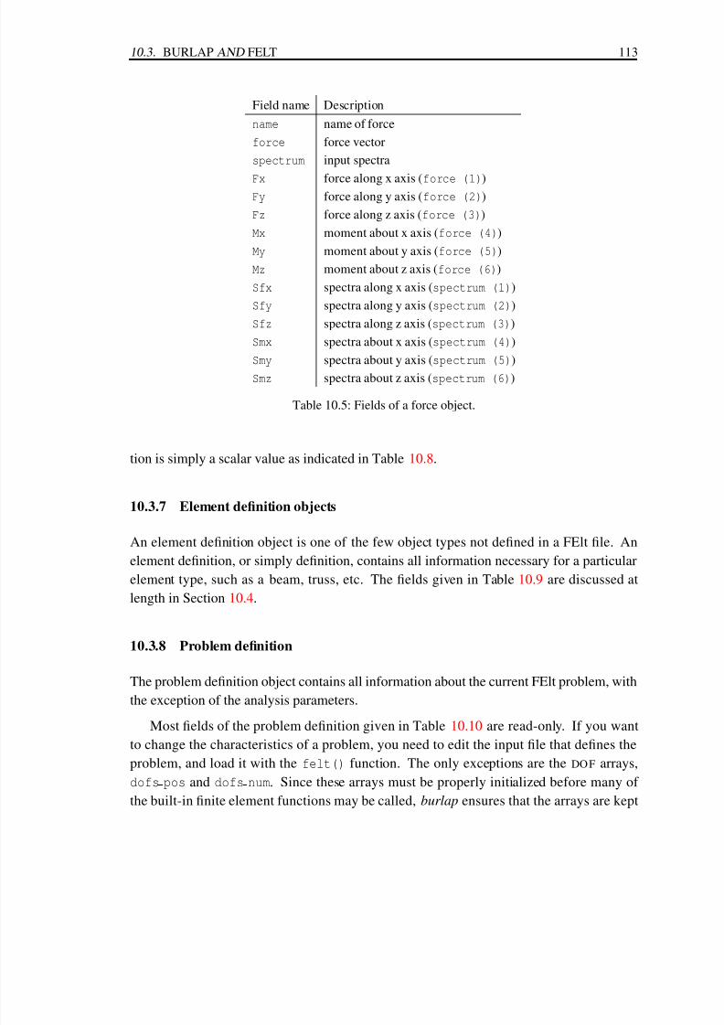
7/30/2019 Felt Manual
http://slidepdf.com/reader/full/felt-manual 135/236
10.3. BURLAP AND FELT 113
Field name Description
name name of force
force force vector
spectrum input spectra
Fx force along x axis (force (1))Fy force along y axis (force (2))
Fz force along z axis (force (3))
Mx moment about x axis (force (4))
My moment about y axis (force (5))
Mz moment about z axis (force (6))
Sfx spectra along x axis (spectrum (1))
Sfy spectra along y axis (spectrum (2))
Sfz spectra along z axis (spectrum (3))
Smx spectra about x axis (spectrum (4))
Smy spectra about y axis (spectrum (5))Smz spectra about z axis (spectrum (6))
Table 10.5: Fields of a force object.
tion is simply a scalar value as indicated in Table 10.8.
10.3.7 Element definition objects
An element definition object is one of the few object types not defined in a FElt file. An
element definition, or simply definition, contains all information necessary for a particular
element type, such as a beam, truss, etc. The fields given in Table 10.9 are discussed at
length in Section 10.4.
10.3.8 Problem definition
The problem definition object contains all information about the current FElt problem, with
the exception of the analysis parameters.
Most fields of the problem definition given in Table 10.10 are read-only. If you want
to change the characteristics of a problem, you need to edit the input file that defines the
problem, and load it with the felt() function. The only exceptions are the DO F arrays,
dofs pos and dofs num. Since these arrays must be properly initialized before many of
the built-in finite element functions may be called, burlap ensures that the arrays are kept

7/30/2019 Felt Manual
http://slidepdf.com/reader/full/felt-manual 136/236
114 CHAPTER 10. THE BURLAP APPLICATION
Field name Description
name name of constraint
constraint constraint vector
ix initial displacement vectorvx initial velocity vector
ax initial acceleration vector
dx boundary displacement vector
iTx initial displacement along x axis (ix (1))
iTy initial displacement along y axis (ix (2))
iTz initial displacement along z axis (ix (3))
iRx initial rotation about x axis (ix (4))
iRy initial rotation about y axis (ix (5))
iRz initial rotation about z axis (ix (6))
Vx initial velocity along x axis (vx (1))
Vy initial velocity along y axis (vx (2))
Vz initial velocity along z axis (vx (3))
Ax initial acceleration along x axis (ax (1))
Ay initial acceleration along y axis (ax (2))
Az initial acceleration along z axis (ax (3))
Tx translation along x axis (dx (1))
Ty translation along y axis (dx (2))
Tz translation along z axis (dx (3))
Rx translation along x axis (dx (4))
Ry translation along y axis (dx (5))
Rz translation along z axis (dx (6))
Table 10.6: Fields of a constraint object.
Field name Description
name name of distributed load
direction load direction
num values number of values
values array of values ((node, magnitude) pairs)
Table 10.7: Fields of a distributed load object.

7/30/2019 Felt Manual
http://slidepdf.com/reader/full/felt-manual 137/236
10.3. BURLAP AND FELT 115
Direction Value
LocalX &local x
LocalY &local y
LocalZ &local z
GlobalX &global x
GlobalY &global y
GlobalZ &global z
Parallel ¶llel
Perpendicular &perpendicular
Table 10.8: Directions of a distributed load.
Field name Description
name name of definitionsetup element set-up function
stress element stress computation function
num nodes number of nodes in element
shape nodes number of nodes that define shape
num dofs number of degrees of freedom
dofs degrees of freedom
num stresses number of stresses
retainK flag to retain stiffness matrix after assembly
Table 10.9: Fields of an element definition object.
Field name Description
mode analysis mode
title problem title
nodes array of node objects
elements array of element object
dofs pos global DO F positions
dofs num global DO F numbers
num dofs number of active DO Fsnum nodes number of nodes
num elements number of elements
Table 10.10: Fields of a problem definition object.
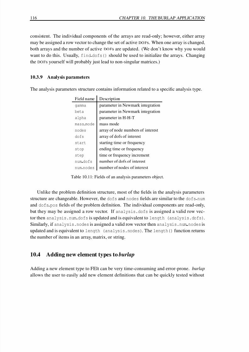
7/30/2019 Felt Manual
http://slidepdf.com/reader/full/felt-manual 138/236
116 CHAPTER 10. THE BURLAP APPLICATION
consistent. The individual components of the arrays are read-only; however, either array
may be assigned a row vector to change the set of active DO Fs. When one array is changed,
both arrays and the number of active DO Fs are updated. (We don’t know why you would
want to do this. Usually, find dofs() should be used to initialize the arrays. Changing
the DO Fs yourself will probably just lead to non-singular matrices.)
10.3.9 Analysis parameters
The analysis parameters structure contains information related to a specific analysis type.
Field name Description
gamma parameter in Newmark integration
beta parameter in Newmark integration
alpha parameter in H-H-T
mass mode mass mode
nodes array of node numbers of interest
dofs array of dofs of interest
start starting time or frequency
stop ending time or frequency
step time or frequency increment
num dofs number of dofs of interest
num nodes number of nodes of interest
Table 10.11: Fields of an analysis parameters object.
Unlike the problem definition structure, most of the fields in the analysis parameters
structure are changeable. However, the dofs and nodes fields are similar to the dofs num
and dofs pos fields of the problem definition. The individual components are read-only,
but they may be assigned a row vector. If analysis.dofs is assigned a valid row vec-
tor then analysis.num dofs is updated and is equivalent to length (analysis.dofs).
Similarly, if analysis.nodes is assigned a valid row vector then analysis.num nodes is
updated and is equivalent to length (analysis.nodes). The length() function returns
the number of items in an array, matrix, or string.
10.4 Adding new element types to burlap
Adding a new element type to FElt can be very time-consuming and error-prone. burlap
allows the user to easily add new element definitions that can be quickly tested without

7/30/2019 Felt Manual
http://slidepdf.com/reader/full/felt-manual 139/236
10.4. ADDING NEW ELEMENT TYPES TO BURLAP 117
having to recompile the felt or velvet applications. To add a new element to the set of ex-
isting elements, the add definition() function is used. Similarly, to remove an existing
element definition, the remove definition() function is used.
Argument Description Type Example
name name of definition string "truss"
set up set up function (K and M ) function truss set up
stress stress computation function function truss stress
shape element shape scalar &linear
num nodes number of nodes in element scalar 2
shape nodes number of nodes that define shape scalar 2
num stresses number of stress values scalar 1
dofs vector of DO Fs row vector [1,2,3,0,0,0]
retainK retain stiffness matrix indicator scalar &false
Table 10.12: Arguments to the add definition() function.
The add definition() function requires a variety of arguments as shown in
Table 10.12. For the reminder of the discussion regarding the arguments to the
add definition() function, we will use the truss element as an example.
The name of the element definition is a string by which the element type is referred.
Once the element definition has been successfully added then new elements of that type
can be created. In our example the name is "truss", so a FElt file can now be loaded that
contains truss elements. If an element definition of the same name already exists then
add definition() returns 1, otherwise it returns 0.
The set up function is a burlap function that will compute the local stiffness matrix,
K , and local mass matrix, M , for any element of the new definition. Our sample set-up
function is shown in Figure 10.1. For our simple truss element, we are ignoring the mass
matrix and the effect of distributed loads.
The set-up function will be called with two arguments. The first argument is the element
whose stiffness and mass matrices are to be computed. The second argument is the mass
mode, which is one of &false, &lumped, or &consistent, where &false indicates that
no mass matrix is required. In our simple example, we have simply omitted the second
argument, since we will not be considering mass matrices. Note that the set up argument
is a burlap function itself, not the name of the function. As discussed in Section 11.6,
functions in burlap are simply variables that can be passed as arguments to functions and
also returned from functions. Our simple function for truss elements computes the length
of the element by calling the length() function, which is discussed in Section 11.5.4.

7/30/2019 Felt Manual
http://slidepdf.com/reader/full/felt-manual 140/236
118 CHAPTER 10. THE BURLAP APPLICATION
function truss_set_up (e)
L = length (e)
AEonL = e.material.A * e.material.E / e.material.L
K = [AEonL, -AEonL; -AEonL, AEonL]
cx = (e.node (2).x - e.node (1).x) / L
cy = (e.node (2).y - e.node (1).y) / L
cz = (e.node (2).z - e.node (1).z) / L
T = [cx, cy, cz, 0, 0, 0; 0, 0, 0, cx, cy, cz]
e.K = T’*K*T
return 0
end
Figure 10.1: Set-up function for the truss element definition.
The set-up function assigns the stiffness and mass matrices to the element by assigning
to the K and M fields of the element structure. If the set-up function is successful then it
should return zero. Otherwise, it should return a non-zero value.
The stress function is a burlap function that will compute the stress values for any
element of the new definition. Our sample set-up function is shown in Figure 10.2. The
stress function assigns the stresses by assigning to the stress field of the element structure.If the stress function is successful then it should return zero. Otherwise, it should return a
non-zero value.
Our simple truss element has only one integration point and only a single stress value at
that point. Since an element may have an arbitrary number of integration points, the ninteg
field of the element structure must be set before the stress vector can be accessed. The
number of stresses and thus the length of the values vector is determined by the element
definition. In the computation of the stress value for the truss element, the two displacement
row vectors are subtracted and then multiplied by the column vector, c, to yield a scalar.
The remaining arguments to add definition() are easily calculated. The shape of our
truss element is linear and has two nodes, both of which are required and needed to define
the shape of the element. The truss element permits displacements along the X, Y, and Z
axes, but does not allow for rotation about any of the axes. Therefore, the first, second, and
third DO Fs are active. The entire call to add definition() is:
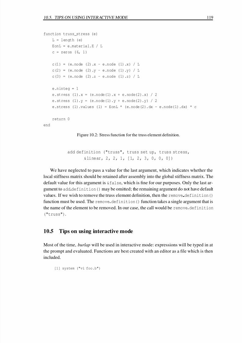
7/30/2019 Felt Manual
http://slidepdf.com/reader/full/felt-manual 141/236
10.5. TIPS ON USING INTERACTIVE MODE 119
function truss_stress (e)
L = length (e)
EonL = e.material.E / L
c = zeros (6, 1)
c(1) = (e.node (2).x - e.node (1).x) / L
c(2) = (e.node (2).y - e.node (1).y) / L
c(3) = (e.node (2).z - e.node (1).z) / L
e.ninteg = 1
e.stress (1).x = (e.node(1).x + e.node(2).x) / 2
e.stress (1).y = (e.node(1).y + e.node(2).y) / 2
e.stress (1).values (1) = EonL * (e.node(2).dx - e.node(1).dx) * c
return 0end
Figure 10.2: Stress function for the truss element definition.
add definition ("truss", truss set up, truss stress,
&linear, 2, 2, 1, [1, 2, 3, 0, 0, 0])
We have neglected to pass a value for the last argument, which indicates whether the
local stiffness matrix should be retained after assembly into the global stiffness matrix. The
default value for this argument is &false, which is fine for our purposes. Only the last ar-
gument to add definition() may be omitted; the remaining argument do not have default
values. If we wish to remove the truss element definition, then the remove definition()
function must be used. The remove definition() function takes a single argument that is
the name of the element to be removed. In our case, the call would be remove definition
("truss").
10.5 Tips on using interactive mode
Most of the time, burlap will be used in interactive mode: expressions will be typed in at
the prompt and evaluated. Functions are best created with an editor as a file which is then
included.
[1] system ("vi foo.b")
7/30/2019 Felt Manual
http://slidepdf.com/reader/full/felt-manual 142/236
120 CHAPTER 10. THE BURLAP APPLICATION
[2] include ("foo.b")
[3] system ("vi foo.b")
[4] include ("foo.b")
It soon becomes tedious to retype the same expressions. If burlap is compiled with thereadline library, then you can use the built-in history mechanism.
[1] system ("vi foo.b")
[2] include ("foo.b")
[3] !s
[4] !i
For those not familiar with csh or bash, !s executes the last line that begins with s.
Similarly, !i executes the last line that begins with i. You can save yourself more typing
by using the word completion abilities of the readline library. Pressing the tab key will
complete the current word. If there is not a unique completion, then you will hear a bell
and pressing the tab key again will list the completions.
[1] sy <Tab>
symmetric? system
[1] system ("vi foo.b")
[2] in <Tab>
in integrate_hyperbolic inv
include integrate_parabolic
[2] include ("foo.b")
The default set of built-in completions includes all keywords such as function and
return, intrinsic functions such as include and sin, and enumeration constants such as
&linear and &null. Inside a quoted string, the default set of completions is not used;
instead, file names are completed.
[1] include ("Examples/f <Tab>
fe.b find-dofs.b foo.flt foo_d.flt
[1] include ("Examples/f
Using the completion mechanism can save a lot of typing, especially when referring to
file names. Another trick is to define your own aliases for common lines.
[1] alias v system ("vi foo.b")
[2] alias vi system ("vi !$")
[3] alias print write (!*)
[4] vi foo.b
7/30/2019 Felt Manual
http://slidepdf.com/reader/full/felt-manual 143/236
10.6. COMMON ERROR MESSAGES 121
The first alias defines v to be system ("vi foo.b"). The second is more general and
defines vi to be system ("vi !$"). The string !$ will be replaced with the last word on
the line. A complete description of the history expansion can be found in the documentation
for the readlinelibrary and for csh. The final alias, print, is simply a convenient wrapper
for the write function.
If burlap is not compiled with the readline library, you still have access to a limited
form of aliasing. The only expansion string legal in an alias is %s which will expand to the
entire line except the first word. A similar alias to vi above would be system ("vi %s").
An alternative to writing aliases is to define your own convenience functions. If
you wish to be able to both edit and include a file then you can write a small function,
called edit, and place it in a file called edit.b in your search path, as described in Sec-
tion 11.4.14.
function edit (s)system (concat ("vi ", s))
include (s)
end
Finally, it is important to realize that the readline library capabilities and aliases work
on lines, not on expressions. History substitutions apply to the lines entered, not to the
individual expressions on a line. Similarly, aliases and history expansion characters are not
recognized when burlap is reading from a file.
10.6 Common error messages
This section attempts to explain some of the common error messages associated with using
burlap. All error messages are prefixed with the name of the file and the number of the
line that was found to be in error. An error on a line may not be discovered until several
lines later, so the line number may not be the line that actually contained the error. If an
error occurs in a function, then the function call is terminated and the error is propagated
back to the outermost level. In this case, the calling sequence is shown to assist in tracking
down the cause of the error. In the examples given, the file name and line number have
been omitted.
type error in expression: function call to null
This error indicates that the function call or array index operators were ap-
plied to a null expression such as foo ( ), where foo is null. This error

7/30/2019 Felt Manual
http://slidepdf.com/reader/full/felt-manual 144/236
122 CHAPTER 10. THE BURLAP APPLICATION
often results from misspelling a variable name or from forgetting to declare
a global variable using the global declaration in a function body. You can
generally locate this error by searching for parentheses on the offending
line.
type error in expression: type has no such field
The field index operator was applied to an object of the specified type, but
the object has no such field. You can generally locate this error by searching
for a period on the given line.
type error in expression: type1 operator type2
The specified operator does not allow operands of the specified types. The
way to fix this error is to determine what operand types are allowed, as
discussed in Section 11.4, and determine why one or more of your operands
are of the incorrect type.
parse error before string
At some time at or before string, the expression syntax was illegal. Often,
string is the cause of the error. You should now be back at the top level
prompt, in which case you can correct your error and try again.
size mismatch in expression: (a x b) operator (c x d )
The types of the operands were legal for the specified operator , but the
sizes of the operands were illegal. The legal operand sizes are discussed in
Section 11.4.

7/30/2019 Felt Manual
http://slidepdf.com/reader/full/felt-manual 145/236
Chapter 11
The burlap Syntax
burlap has a rich variety of operators and functions for manipulating matrices, scalars,strings, and FElt objects. Matrices are denoted by square brackets with matrix elements
separated by commas and matrix rows separated by semicolons. Scalars are floating-point
numbers such as 3.14159 or 123. Any scalar can also be converted to a matrix with one
row and one column. Strings are enclosed in double quotation marks. Special enumeration
constants begin with an ampersand, as in &local x. Variable names are a sequence of
letters, digits, and the underscore character. Finally, comments are enclosed within /* */;
a pound sign (#) may also be used to indicate a comment until the end of the current line.
[1] a = 3.14159
[2] b = "hello"
[3] c = [1, 2, 3; 4, 5, 6]
[4] write (a)
3.14159
[5] write (b)
hello
[6] write (c)
1 2 3
4 5 6
The following sections discuss the operators and functions of burlap in detail. They
are intended to be the definitive word on the semantics of the operators, functions, matrix
formers, etc.
123

7/30/2019 Felt Manual
http://slidepdf.com/reader/full/felt-manual 146/236
124 CHAPTER 11. THE BURLAP SYNTAX
11.1 Literals
It seems appropriate to begin the discussion with the literals since they are the building
blocks of the burlap syntax. As previously mentioned, floating-point literals are numbers
such as 123 or 3.14159. Specifically, a numeric literal consists of a base followed by an
optional exponent . The base consists of a series of digits with an optional decimal point.
The exponent consists of the letter E or e followed by the digits of the base-10 exponent.
The digits in the exponent may be preceded by a + or - to indicate a positive or negative
exponent, respectively. String literals are enclosed within double quotation marks, as in
"hello". The following escapes may be used to introduce special characters within a
string literal.
audible alert \a carriage return \r
backspace \b horizontal tab \t
formfeed \f vertical tab \v
newline \n quote \"
Matrices are delimited by square brackets with rows separated by semicolons and el-
ements within a row separated by commas. An important thing to realize when writing
matrices is that burlap may automatically insert a semicolon at the end of line. In particu-
lar, a semicolon is inserted at the end of a line in interactive mode when the last literal or
operator on the line can end an expression.
[ 1 ] a = [ 1 , 2 , 3[2] 4, 5, 6]
[3] write (a)
1 2 3
4 5 6
[ 4 ] a = [ 1 , 2 , 3 +
4> 4, 5, 6]
[5] write (a)
1 2 7 5 6
Note that since an expression cannot end with +, the next line is taken to be a continu-
ation of the previous line. A matrix element may be an arbitrary expression; however, all
expressions on the same row must have the same height. Additionally, all rows must have
the same number of columns.

7/30/2019 Felt Manual
http://slidepdf.com/reader/full/felt-manual 147/236
11.2. VARIABLES 125
[ 1 ] x = 1
[2] a = [0, x, 2]
[3] write (a)
0 1 2
[4] b = [a; 3, 4, 5]
[5] write (b)
0 1 2
3 4 5
[6] write ([b, b])
0 1 2 0 1 2
3 4 5 3 4 5
[7] write ([b, a])
stdin:7: inconsistent number of rows
11.2 Variables
Variables are named by a sequence of letters, digits, the underscore character, and the
question mark symbol. A variable must begin with a letter or the underscore character. The
question mark may only appear as the last character in a variable name. There is no limit
on the length of a variable name.
Variables are assigned values either through the assignment operator, parameter pass-
ing, or function definitions. A variable is either local or global. Local variables are those
variables referenced within a function body. Global variables are those variables referenced
outside a function body. To explicitly reference a global variable inside a function body, it
must be declared as global using the global declaration.
function foo (x)
global y, z
r e t u r n x + y + z
end
The function foo references two global variables, y and z. If the function did not use
the global declaration then y and z would be local variables. The only exception to this
rule is a function call, as discussed in Section 11.4.14.
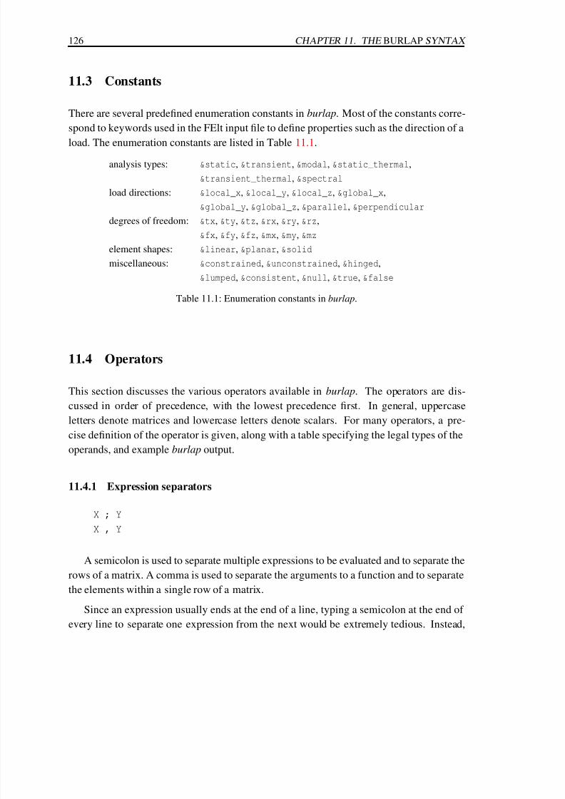
7/30/2019 Felt Manual
http://slidepdf.com/reader/full/felt-manual 148/236
126 CHAPTER 11. THE BURLAP SYNTAX
11.3 Constants
There are several predefined enumeration constants in burlap. Most of the constants corre-
spond to keywords used in the FElt input file to define properties such as the direction of a
load. The enumeration constants are listed in Table 11.1.
analysis types: &static, &transient, &modal, &static_thermal,
&transient_thermal, &spectral
load directions: &local_x, &local_y, &local_z, &global_x,
&global_y, &global_z, ¶llel, &perpendicular
degrees of freedom: &tx, &ty, &tz, &rx, &ry, &rz,
&fx, &fy, &fz, &mx, &my, &mz
element shapes: &linear, &planar, &solid
miscellaneous: &constrained, &unconstrained, &hinged,
&lumped, &consistent, &null, &true, &false
Table 11.1: Enumeration constants in burlap.
11.4 Operators
This section discusses the various operators available in burlap. The operators are dis-
cussed in order of precedence, with the lowest precedence first. In general, uppercase
letters denote matrices and lowercase letters denote scalars. For many operators, a pre-cise definition of the operator is given, along with a table specifying the legal types of the
operands, and example burlap output.
11.4.1 Expression separators
X ; Y
X , Y
A semicolon is used to separate multiple expressions to be evaluated and to separate therows of a matrix. A comma is used to separate the arguments to a function and to separate
the elements within a single row of a matrix.
Since an expression usually ends at the end of a line, typing a semicolon at the end of
every line to separate one expression from the next would be extremely tedious. Instead,

7/30/2019 Felt Manual
http://slidepdf.com/reader/full/felt-manual 149/236
11.4. OPERATORS 127
burlap will automatically insert a semicolon for you at the end of a line under certain
conditions. When reading from a terminal in interactive mode, if the last token on the line
may end an expression then a semicolon is inserted. When reading from a file, if the last
token on the line may end an expression and the first token on the next line may begin an
expression then a semicolon will be inserted. A line can be explicitly continued by endingthe line with a backslash character.
[1] write ("hello"); write ("there")
hello
there
[ 2 ] a = 1 +
2> 2 + 3
[3] write (a)
6
[ 4 ] b = 1 \
4 > + 2
[5] write (b)
3
[ 6 ] x = [ 1 , 2 , 3
[7] 4, 5, 6]
[8] write (x)
1 2 3
4 5 6
Although these semantics may sound complicated, they are designed so that 99.9% of
the time you don’t need to worry about when to add a semicolon. However, if you find
yourself with a nasty bug, you might want to review the rules for inserting semicolons or
try putting in an explicit semicolon or backslash.
11.4.2 Assignment expressions
X = Y ; X : = Y
The assignment operator has two equivalent forms and groups from right-to-left. An as-signment expression assigns Y to X and returns X . X must be a variable name, a submatrix,
a field reference, or the result of a function call returning a global variable.
Generally, any expression can be assigned to a variable. However, in certain cases the
expression on the right-hand side is restricted. For example, if X is a submatrix, created as

7/30/2019 Felt Manual
http://slidepdf.com/reader/full/felt-manual 150/236
128 CHAPTER 11. THE BURLAP SYNTAX
the result of indexing a matrix, then the dimensions (number of rows and columns) of X
and Y must agree.
If X is the result of a field reference of a FElt structure then there may be type constraints
on Y . For example, a matrix cannot be assigned to the component of a force. Some fields
are also read-only, such as the name of a constraint or the number of a node or element.
[1] a = [1, 2, 3]
[2] write (a)
1 2 3
[ 3 ] a = b = 0
[4] write (a, " ", b)
0 0
[ 5 ] a = ( b = 2 ) + 1
[6] write (a, " ", b)
3 2
[7] nodes (1).number = 3
stdin:7: type error in expression: changing a read-only variable
[8] nodes (1).force.Fx = 4
[9] nodes (1).force.Fy = [1, 2, 3]
stdin:9: type error in expression: scalar = matrix
[10] a = [1, 2, 3; 4, 5, 6]
[11] write (a)
1 2 3
4 5 6
[12] a (1, 2) = 0
[13] write (a)
1 0 3
4 5 6
11.4.3 Logical OR operator
x o r y ; x | | y
The logical OR operator has two equivalent forms and groups from left-to-right. It
returns 1 if either of its operands compares unequal to zero, and 0 otherwise. The OR
operator guarantees left-to-right evaluation: x is first evaluated; if it is unequal to 0, the
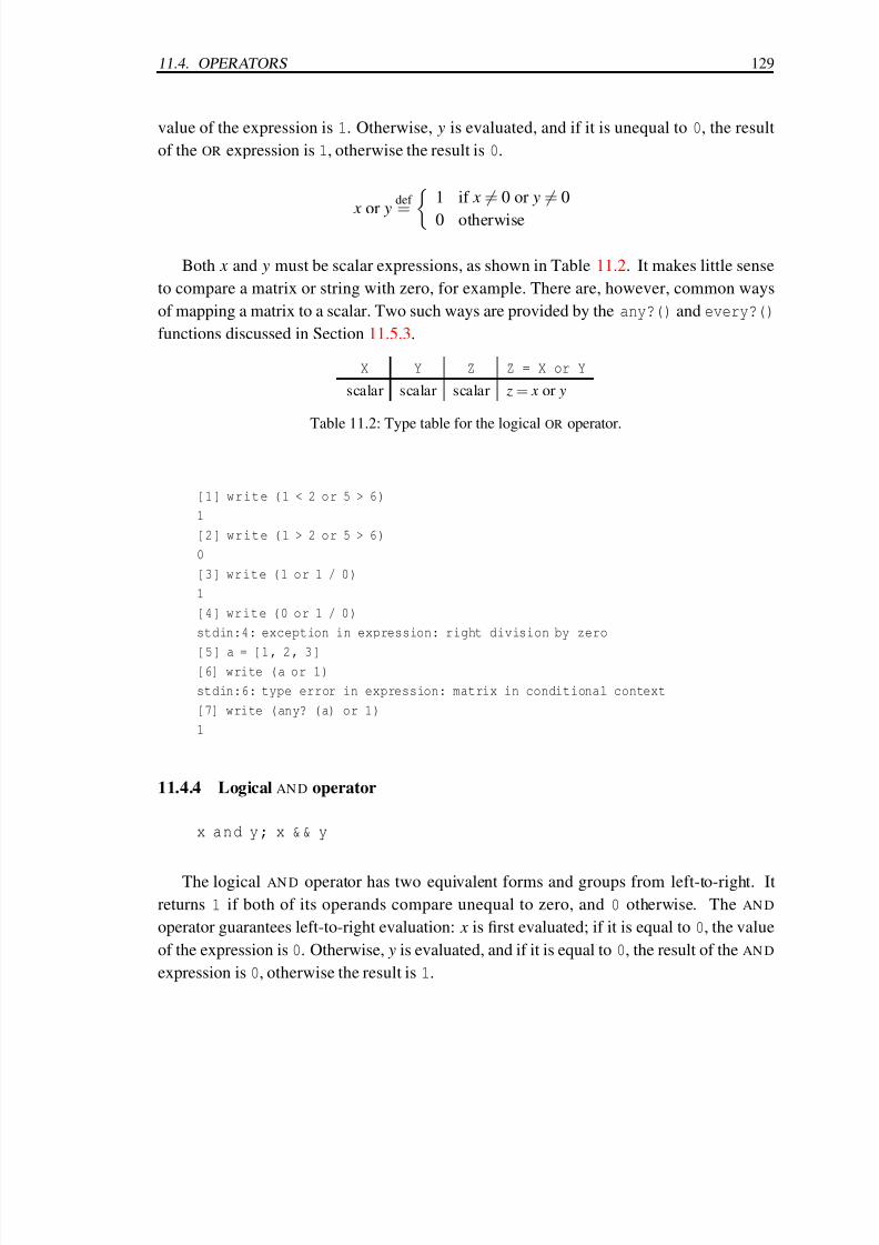
7/30/2019 Felt Manual
http://slidepdf.com/reader/full/felt-manual 151/236
11.4. OPERATORS 129
value of the expression is 1. Otherwise, y is evaluated, and if it is unequal to 0, the result
of the OR expression is 1, otherwise the result is 0.
x or ydef = 1 if x
= 0 or y
= 0
0 otherwise
Both x and y must be scalar expressions, as shown in Table 11.2. It makes little sense
to compare a matrix or string with zero, for example. There are, however, common ways
of mapping a matrix to a scalar. Two such ways are provided by the any?() and every?()
functions discussed in Section 11.5.3.
X Y Z Z = X or Y
scalar scalar scalar z = x or y
Table 11.2: Type table for the logical OR operator.
[1] write (1 < 2 or 5 > 6)
1
[2] write (1 > 2 or 5 > 6)
0
[3] write (1 or 1 / 0)
1
[4] write (0 or 1 / 0)
stdin:4: exception in expression: right division by zero
[5] a = [1, 2, 3][6] write (a or 1)
stdin:6: type error in expression: matrix in conditional context
[7] write (any? (a) or 1)
1
11.4.4 Logical AN D operator
x a n d y ; x & & y
The logical AN D operator has two equivalent forms and groups from left-to-right. It
returns 1 if both of its operands compare unequal to zero, and 0 otherwise. The AN D
operator guarantees left-to-right evaluation: x is first evaluated; if it is equal to 0, the value
of the expression is 0. Otherwise, y is evaluated, and if it is equal to 0, the result of the AN D
expression is 0, otherwise the result is 1.

7/30/2019 Felt Manual
http://slidepdf.com/reader/full/felt-manual 152/236
130 CHAPTER 11. THE BURLAP SYNTAX
x and ydef =
1 if x = 0 and y = 0
0 otherwise
Both x and y must be scalar expressions, as shown in Table 11.3. It makes little senseto compare a matrix or string with zero, for example. There are, however, common ways
of mapping a matrix to a scalar. Two such ways are provided by the any?() and every?()
functions discussed in Section 11.5.3.
X Y Z Z = X and Y
scalar scalar scalar z = x and y
Table 11.3: Type table for the logical AN D operator.
[1] write (1 < 2 and 3 < 4)
1
[2] write (1 < 2 and 3 > 4)
0
[3] write (0 and 1 / 0)
0
[4] write (1 and 1 / 0)
stdin:4: exception in expression: right division by zero
11.4.5 Equality operators
X = = Y
X ! = Y ; X < > Y
The equality (==) and inequality (!= or <>) operators associate from left-to-right. The
result of the expression is 1 if true, and 0 if false.
x = ydef =
1 if x = y
0 otherwise
x != ydef =
1 if x = y
0 otherwise
Unlike the previously discussed operators, these operators, like most of the operators in
burlap, accept a variety of types as operands, as shown in Table 11.4.

7/30/2019 Felt Manual
http://slidepdf.com/reader/full/felt-manual 153/236
11.4. OPERATORS 131
X Y Z Z = X op Y
matrix matrix matrix ∀i, j | Z i, j = X i, j op Y i, j
matrix scalar matrix ∀i, j | Z i, j = X i, j op y
scalar matrix matrix ∀i, j | Z i, j = x op Y i, j
scalar scalar scalar z = x op y (scalar comparison)string string scalar z = x op y (lexicographic comparison)
object object scalar z = x op y (object identity comparison)
Table 11.4: Type table for the equality operators.
Although the table might look confusing, it provides a precise semantics for all possible
type operands. Essentially, burlap does element-by-element comparison for matrices and
scalars, string (i.e., lexicographic) comparison for strings, and identity (i.e., pointer) com-
parison on all other type objects. When comparing two matrices, their dimensions must beidentical.
[1] write ([1, 2, 3] == 2)
0 1 0
[2] write (2 != [1, 2, 3])
1 0 1
[3] write ([1, 2, 3] == [3, 2, 3])
0 1 1
[4] write ("hello" == "hello")
1
[5] write ("hello" == "there")
0
[6] write (nodes (1) == nodes (1))
1
[7] write (nodes (1) == elements (1))
stdin:7: type error in expression: node == element
11.4.6 Relational operators
X < Y

7/30/2019 Felt Manual
http://slidepdf.com/reader/full/felt-manual 154/236
132 CHAPTER 11. THE BURLAP SYNTAX
X > Y
X < = Y
X > = Y
The relational operators are similar to the equality operators, with the only differencebeing that they do not allow an arbitrary object type as an operand for comparison (Ta-
ble 11.5).
X Y Z Z = X op Y
matrix matrix matrix ∀i, j | Z i, j = X i, j op Y i, j
matrix scalar matrix ∀i, j | Z i, j = X i, j op y
scalar matrix matrix ∀i, j | Z i, j = x op Y i, j
scalar scalar scalar z = x op y (scalar comparison)
string string scalar z = x op y (lexicographic comparison)
Table 11.5: Type table for the relational operators.
The result of the expression is 1 if the expression is true, and 0 if the expression is false.
If two matrices are compared, then their dimensions must be identical.
[1] write ([1, 2, 3] < 3)
1 1 0
[2] write ([1, 2, 3] >= [3, 2, 1])
0 1 1
[3] write ("aardvark" < "aardwolf")
1
11.4.7 Range operator
x : z
x : y : z
The range operator produces a row vector starting at x and ending at z, with y used as
the step between successive elements.
x : y : zdef =
x x + y · · · x +
z− x
y
y
if ( x ≤ z and y > 0) or ( x ≥ z and y < 0)
null otherwise

7/30/2019 Felt Manual
http://slidepdf.com/reader/full/felt-manual 155/236
11.4. OPERATORS 133
If y is not specified then 1 is used as the step value. Each of x, y, and z must be scalar
expressions, as shown in Table 11.6.
X Y Z W W = X : Y : Z
scalar scalar scalar matrix (as defined above)
Table 11.6: Type table for the range operator.
[1] write (1:3)
1 2 3
[2] write (3:1)
null
[3] write (1:2:10)
1 3 5 7 9
[4] write (10:-2:1)
10 8 6 4 2
As illustrated above, if the range is improperly specified then a null value is returned.
The null value is illegal in most operations and is used to indicate an uninitialized value.
11.4.8 Additive operators
X + Y
X - Y
The type semantics of the additive operators are quite similar to the semantics of the
relational and equality operators, except that only scalars and matrices are allowed. As
shown in Table 11.7, adding two scalars produces a scalar, as expected; adding a matrix to
a scalar simply adds the scalar to each element of the matrix; adding two matrices results
in standard matrix addition, again as expected.
Like the equality and relational operators, the additive operators associate from left-to-
right. Also, two matrices must have identical dimensions for addition or subtraction.
[1] write (1 + 2)
3
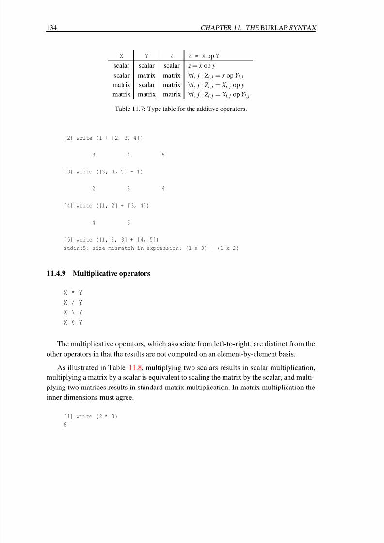
7/30/2019 Felt Manual
http://slidepdf.com/reader/full/felt-manual 156/236
134 CHAPTER 11. THE BURLAP SYNTAX
X Y Z Z = X op Y
scalar scalar scalar z = x op y
scalar matrix matrix ∀i, j | Z i, j = x op Y i, j
matrix scalar matrix ∀i, j | Z i, j = X i, j op y
matrix matrix matrix ∀i, j | Z i, j = X i, j op Y i, j
Table 11.7: Type table for the additive operators.
[2] write (1 + [2, 3, 4])
3 4 5
[3] write ([3, 4, 5] - 1)
2 3 4
[4] write ([1, 2] + [3, 4])
4 6
[5] write ([1, 2, 3] + [4, 5])
stdin:5: size mismatch in expression: (1 x 3) + (1 x 2)
11.4.9 Multiplicative operators
X * Y
X / Y
X \ Y
X % Y
The multiplicative operators, which associate from left-to-right, are distinct from the
other operators in that the results are not computed on an element-by-element basis.
As illustrated in Table 11.8, multiplying two scalars results in scalar multiplication,
multiplying a matrix by a scalar is equivalent to scaling the matrix by the scalar, and multi-plying two matrices results in standard matrix multiplication. In matrix multiplication the
inner dimensions must agree.
[1] write (2 * 3)
6
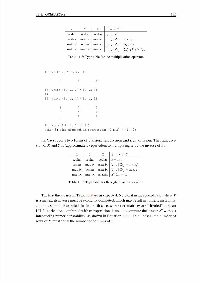
7/30/2019 Felt Manual
http://slidepdf.com/reader/full/felt-manual 157/236
11.4. OPERATORS 135
X Y Z Z = X * Y
scalar scalar scalar z = x × y
scalar matrix matrix ∀i, j | Z i, j = x ×Y i, j
matrix scalar matrix ∀i, j | Z i, j = X i, j × y
matrix matrix matrix ∀i, j | Z i, j = ∑nk =1 X i,k ×Y k , j
Table 11.8: Type table for the multiplication operator.
[2] write (2 * [1, 2, 3])
2 4 6
[3] write ([1, 2, 3] * [1; 2; 3])
14
[4] write ([1; 2; 3] * [1, 2, 3])
1 2 3
2 4 6
3 6 9
[5] write ([1, 2] * [3, 4])
stdin:5: size mismatch in expression: (1 x 2) * (1 x 2)
burlap supports two forms of division: left division and right division. The right divi-
sion of X and Y is (approximately) equivalent to multiplying X by the inverse of Y .
X Y Z Z = X / Y
scalar scalar scalar z = x/ y
scalar matrix matrix ∀i, j | Z i, j = x ×Y −1i, j
matrix scalar matrix ∀i, j | Z i, j = X i, j/ y
matrix matrix matrix Z | ZY = X
Table 11.9: Type table for the right division operator.
The first three cases in Table 11.9 are as expected. Note that in the second case, where Y
is a matrix, its inverse must be explicitly computed, which may result in numeric instability
and thus should be avoided. In the fourth case, where two matrices are “divided”, then an
LU-factorization, combined with transposition, is used to compute the “inverse” without
introducing numeric instability, as shown in Equation 11.1. In all cases, the number of
rows of X must equal the number of columns of Y .
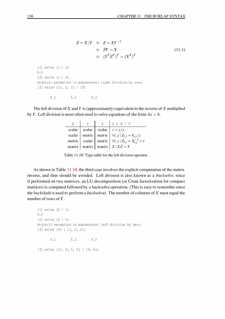
7/30/2019 Felt Manual
http://slidepdf.com/reader/full/felt-manual 158/236
136 CHAPTER 11. THE BURLAP SYNTAX
Z = X /Y ≡ Z = XY −1
≡ ZY = X (11.1)
≡ (Y T Z T )T = ( X T )T
[1] write (1 / 2)
0.5
[2] write (1 / 0)
stdin:2: exception in expression: right division by zero
[3] write ([1, 2, 3] / 10)
0.1 0.2 0.3
The left division of X and Y is (approximately) equivalent to the inverse of X multiplied
by Y . Left division is most often used to solve equations of the form Ax = b.
X Y Z Z = X \ Y
scalar scalar scalar z = y/ x
scalar matrix matrix ∀i, j | Z i, j = Y i, j/ x
matrix scalar matrix ∀i, j | Z i, j = X −1i, j × y
matrix matrix matrix Z | X Z = Y
Table 11.10: Type table for the left division operator.
As shown in Table 11.10, the third case involves the explicit computation of the matrix
inverse, and thus should be avoided. Left division is also known as a backsolve, since
if performed on two matrices, an LU-decomposition (or Crout factorization for compact
matrices) is computed followed by a backsolve operation. (This is easy to remember since
the back slash is used to perform a back solve). The number of columns of X must equal the
number of rows of Y .
[1] write (2 \ 1)
0.5
[2] write (0 \ 1)
stdin:2: exception in expression: left division by zero
[3] write (10 \ [1, 2, 3])
0.1 0.2 0.3
[4] write ([1, 2; 3, 4] \ [5, 6])

7/30/2019 Felt Manual
http://slidepdf.com/reader/full/felt-manual 159/236
11.4. OPERATORS 137
stdin:4: size mismatch in expression: (2 x 2) \ (1 x 2)
[5] write ([1, 2; 3, 4] \ [5; 6])
-4
4.5
Finally, burlap also supports a remainder operation as shown in Table 11.11. In the left
division, right division, and remainder operators, a division by zero will cause a mathemat-
ical exception.
x mod ydef = x − x/ y y
X Y Z Z = X % Y
scalar scalar scalar z = x mod y
scalar matrix matrix ∀i, j | Z i, j = x mod Y i, j
matrix scalar matrix ∀i, j | Z i, j = X i, j mod y
matrix matrix matrix ∀i, j | Z i, j = X i, j mod Y i, j
Table 11.11: Type table for the remainder operator.
11.4.10 Exponentiation operator
x * * y ; x ˆ y
The exponentiation operator has two equivalent forms as associated from right-to-left.
Both x and y must be scalar expressions, as shown in Table 11.12.
x y z z = x ** y
scalar scalar scalar z = x y
Table 11.12: Type table for the exponentiation operator.
Additionally, x must be non-negative or y must be an integer; otherwise a mathematical
exception will result.
[1] write (2 ** 3)
8
[2] write (2 ** .5)
1.41421
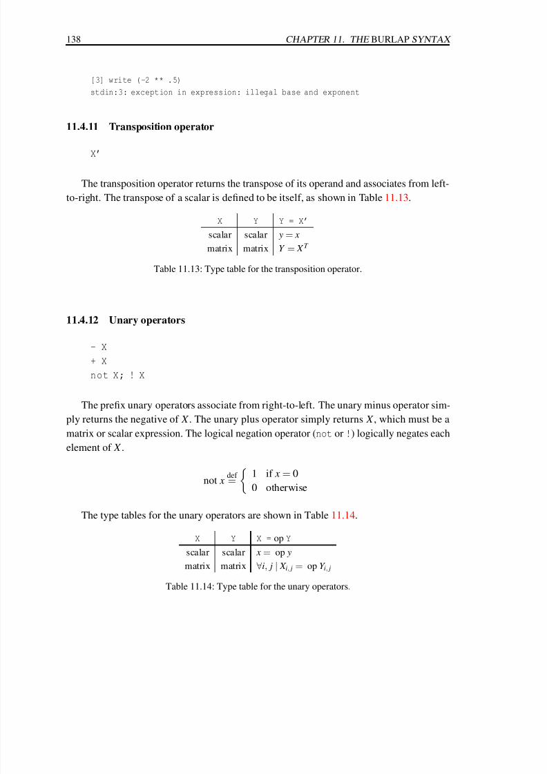
7/30/2019 Felt Manual
http://slidepdf.com/reader/full/felt-manual 160/236
138 CHAPTER 11. THE BURLAP SYNTAX
[3] write (-2 ** .5)
stdin:3: exception in expression: illegal base and exponent
11.4.11 Transposition operator
X’
The transposition operator returns the transpose of its operand and associates from left-
to-right. The transpose of a scalar is defined to be itself, as shown in Table 11.13.
X Y Y = X’
scalar scalar y = x
matrix matrix Y = X T
Table 11.13: Type table for the transposition operator.
11.4.12 Unary operators
- X
+ X
not X; ! X
The prefix unary operators associate from right-to-left. The unary minus operator sim-ply returns the negative of X . The unary plus operator simply returns X , which must be a
matrix or scalar expression. The logical negation operator (not or !) logically negates each
element of X .
not xdef =
1 if x = 0
0 otherwise
The type tables for the unary operators are shown in Table 11.14.
X Y X = op Yscalar scalar x = op y
matrix matrix ∀i, j | X i, j = op Y i, j
Table 11.14: Type table for the unary operators.

7/30/2019 Felt Manual
http://slidepdf.com/reader/full/felt-manual 161/236
11.4. OPERATORS 139
11.4.13 Index expressions
X (I)
X (I,J)
An index expression is used to access the components of matrices. Each index must be
an expression that is either a scalar, a vector whose elements are contiguous and increasing,
or the special vector :, which is used to specify all rows or columns of a matrix and should
not be confused with the range operator. If I or J is a vector then it specifies a range of
indices that are to be used. Thus, : is a shorthand for writing 1 : rows (X) for I or
1 : cols (X) for J .
If X is a matrix then X(i) is its ith column and X(i,j) is the value of the element of
its ith row and jth column. However, if X is a vector then X(i) is its ith element. Since a
scalar is a matrix with one row and one column, it may also be indexed.
[1] A = [1, 2, 3; 4, 5, 6]
[2] x = [1; 2; 3]
[3] y = [1, 2, 3]
[4] write (A)
1 2 3
4 5 6
[5] write (A(2))
2
5
[6] write (A(2,3))
6
[7] write (x)
1
2
3
[8] write (x(2))
2
[9] write (y)
1 2 3

7/30/2019 Felt Manual
http://slidepdf.com/reader/full/felt-manual 162/236
140 CHAPTER 11. THE BURLAP SYNTAX
[10] write (y(1))
1
[11] write (A(:,[2,3]))
2 3
5 6
Thus, there is some ambiguity in using X(i) since if X is a column vector then the result
will be its ith element and if X is a matrix then the result will be its ith column. Therefore,
caution should be used; octave does not support indexing a matrix with a single index.
However, the single index notation can be useful and is consistent with the semantics of the
for expression of Section 11.7.3.
11.4.14 Function expressions
F (...)
A function call is an expression, F , followed by parentheses containing a possibly
empty, comma-separated list of arguments, which may be arbitrary expressions. The ar-
gument list is evaluated in order from left to right. The result of the expression is the return
value of the function named by F . If more arguments are specified than required by the
function, the extra arguments are simply discarded. If too few arguments are specified, then
null values are appended to the argument list. Thus, it is impossible to distinguish a null
value due to an uninitialized variable from a missing argument.
If F evaluates to null and is an identifier, such as write, then the global scope is
searched for a function called F. If a function exists then it is executed. Otherwise, the
directories named by the environment variable BURLAP PATH are searched in order for a file
named first F and then F.b. If a file is found then it is processed just as if include() were
called. After the file is processed the global scope is searched again. If the function still
cannot be found then a type error results. This is the only case in which a global variable
used inside a function does not need to be explicitly declared in a global declaration.
11.5 Intrinsic functions
The intrinsic functions are those functions that are burlap provides by default. They are,
however, just variables and their values can be reassigned, although this is not typically
done. The functions can be grouped into five basic categories:
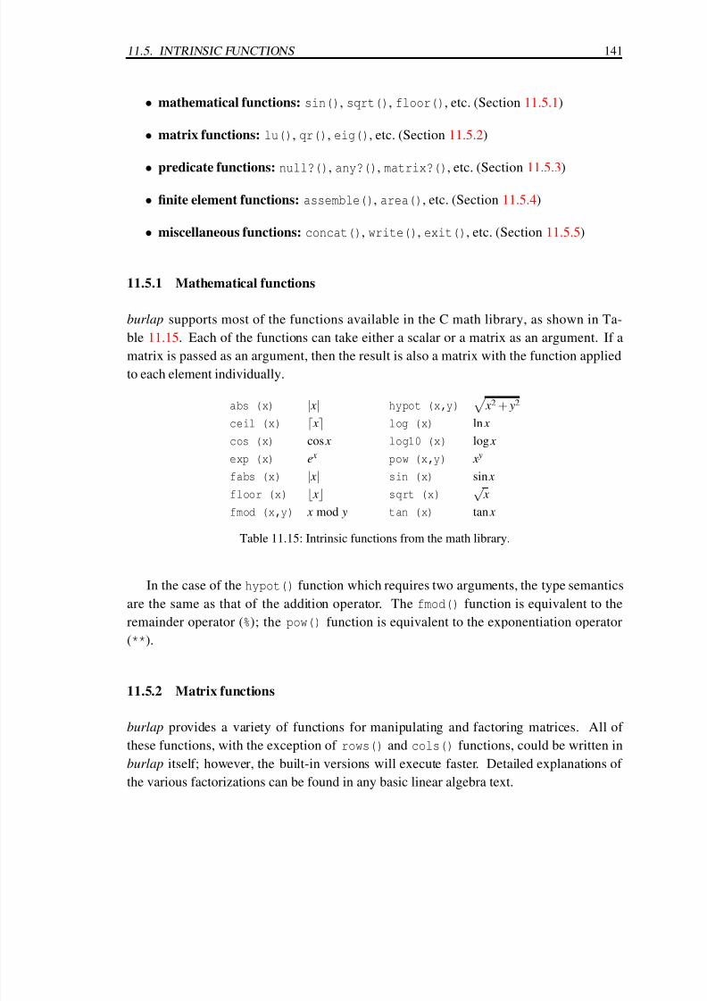
7/30/2019 Felt Manual
http://slidepdf.com/reader/full/felt-manual 163/236
11.5. INTRINSIC FUNCTIONS 141
• mathematical functions: sin(), sqrt(), floor(), etc. (Section 11.5.1)
• matrix functions: lu(), qr(), eig(), etc. (Section 11.5.2)
•predicate functions: null?(), any?(), matrix?(), etc. (Section 11.5.3)
• finite element functions: assemble(), area(), etc. (Section 11.5.4)
• miscellaneous functions: concat(), write(), exit(), etc. (Section 11.5.5)
11.5.1 Mathematical functions
burlap supports most of the functions available in the C math library, as shown in Ta-
ble 11.15. Each of the functions can take either a scalar or a matrix as an argument. If a
matrix is passed as an argument, then the result is also a matrix with the function applied
to each element individually.
abs (x) | x| hypot (x,y)
x2 + y2
ceil (x) x log (x) ln x
cos (x) cos x log10 (x) log x
exp (x) e x pow (x,y) x y
fabs (x) | x| sin (x) sin x
floor (x) x sqrt (x)√
x
fmod (x,y) x mod y tan (x) tan x
Table 11.15: Intrinsic functions from the math library.
In the case of the hypot() function which requires two arguments, the type semantics
are the same as that of the addition operator. The fmod() function is equivalent to the
remainder operator (%); the pow() function is equivalent to the exponentiation operator
(**).
11.5.2 Matrix functions
burlap provides a variety of functions for manipulating and factoring matrices. All of
these functions, with the exception of rows() and cols() functions, could be written in
burlap itself; however, the built-in versions will execute faster. Detailed explanations of
the various factorizations can be found in any basic linear algebra text.

7/30/2019 Felt Manual
http://slidepdf.com/reader/full/felt-manual 164/236
142 CHAPTER 11. THE BURLAP SYNTAX
chol (X) Returns the cholesky factorization of X . The cholesky decomposition of a
matrix X is a matrix B such that BBT = X , provided that X is symmetric
and positive definite. The cholesky decomposition of a scalar is simply its
square root.
cols (X) Returns the number of columns of the matrix X . A scalar is defined to have
a single column. A synonym for this function is columns().
compact (X)
Returns a compact-column matrix whose elements are identical to those of
X , provided that X is a symmetric matrix. Matrices are normally full matri-
ces, with the size of an m × n full matrix requiring O(mn) space. The space
required by a compact-column matrix is approximately equal to the num-
ber of non-zero entries. Most of the FElt functions expect compact-column
matrices. The compact representation of a scalar is itself.
det (X) Returns the determinant of X , | X |, provided that X is a nonsingular matrix.
The determinant of a scalar is itself.
eig (X, V) Returns a column vector, Λ, containing the eigenvalues of X , provided that
X is a square matrix. Therefore, ∀i ∃ y | X y =Λi y. If a variable V is specified
and X is a symmetric matrix then V will contain the matrix of eigenvectors
on return. Each column of V will contain a single eigenvector. Therefore,
∀i | XV i = ΛiV i. If V is missing or X is not a symmetric matrix then only the
eigenvalues are returned.
eye (m, n) Returns an identity matrix of size m × n, I mn. If n is omitted then an m × m
matrix is returned. Both m and n must be scalar expressions that are greater
than zero.
inv (X) Returns the inverse of X ( X −1), which must be either a nonsingular matrix
or a non-zero scalar.
lu (X, L, U, P)
Computes the LU decomposition of X , which must be a nonsingular ma-
trix. The return value is a row permuted superposition of L and U , with thediagonal of L not being stored since L is unit lower triangular. Thus, the
result is not very useful. However, if L is specified as an argument, it will
contain the unit lower triangular matrix on return. Similarly, U will contain
the upper triangular matrix and P will contain the permutation matrix, such
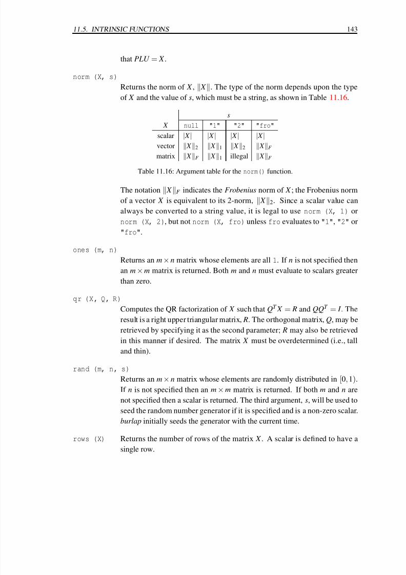
7/30/2019 Felt Manual
http://slidepdf.com/reader/full/felt-manual 165/236
11.5. INTRINSIC FUNCTIONS 143
that PLU = X .
norm (X, s)
Returns the norm of X , X . The type of the norm depends upon the type
of X and the value of s, which must be a string, as shown in Table 11.16.
s
X null "1" "2" "fro"
scalar | X | | X | | X | | X |vector X 2 X 1 X 2 X F
matrix X F X 1 illegal X F
Table 11.16: Argument table for the norm() function.
The notation X F indicates the Frobenius norm of X ; the Frobenius norm
of a vector X is equivalent to its 2-norm, X 2. Since a scalar value canalways be converted to a string value, it is legal to use norm (X, 1) or
norm (X, 2), but not norm (X, fro) unless fro evaluates to "1", "2" or
"fro".
ones (m, n)
Returns an m × n matrix whose elements are all 1. If n is not specified then
an m × m matrix is returned. Both m and n must evaluate to scalars greater
than zero.
qr (X, Q, R)Computes the QR factorization of X such that QT X = R and QQT = I . The
result is a right upper triangular matrix, R. The orthogonal matrix, Q, may be
retrieved by specifying it as the second parameter; R may also be retrieved
in this manner if desired. The matrix X must be overdetermined (i.e., tall
and thin).
rand (m, n, s)
Returns an m × n matrix whose elements are randomly distributed in [0,1).
If n is not specified then an m × m matrix is returned. If both m and n are
not specified then a scalar is returned. The third argument, s, will be used toseed the random number generator if it is specified and is a non-zero scalar.
burlap initially seeds the generator with the current time.
rows (X) Returns the number of rows of the matrix X . A scalar is defined to have a
single row.
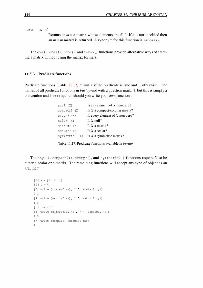
7/30/2019 Felt Manual
http://slidepdf.com/reader/full/felt-manual 166/236

7/30/2019 Felt Manual
http://slidepdf.com/reader/full/felt-manual 167/236
11.5. INTRINSIC FUNCTIONS 145
11.5.4 Finite element functions
The finite element functions provide an interface to the functions in the FElt library. The
functions can all be written in burlap itself, but the built-in functions will execute faster.
add definition (...)
Adds a new element definition. After the definition is added, elements of
that particular type can be loaded using the felt() function. The types
of the arguments are given in order in Table 11.18. Examples and a more
in-depth discussion of the arguments can be found in Section 10.4.
name of definition string
set up function (K and M ) function
stress computation function function
element shape scalar
number of nodes in element scalar
number of nodes that define shape scalar
number of stress values scalar
vector of DO Fs row vector
retain stiffness matrix indicator scalar
Table 11.18: Arguments to the add definition() function.
area (e) Returns the area of the element e. The element must be a planar element
(i.e., e.definition.shape should be &planar).
assemble (M, C)
Computes and returns the global stiffness matrix, K , for the currently de-
fined FElt problem by computing the local stiffness matrices and assembling
them into the global matrix. For transient problems, if M is specified then
it will contain the global mass matrix on return. Similarly, C will contain
the global damping matrix. All matrices are compact-column matrices. The
DO F-related fields of the problem structure must be initialized, as by callingthe find dofs() function.
clear nodes ( )
Clears the displacements and equivalent nodal force vectors for all nodes
defined in the current FElt problem. The return value is null.

7/30/2019 Felt Manual
http://slidepdf.com/reader/full/felt-manual 168/236
146 CHAPTER 11. THE BURLAP SYNTAX
compute modes (K, M, X)
Computes the modes for given stiffness matrix, K , and mass matrix, M . The
result is the vector of eigenvalues, Λ. If X is specified then it will contain
the matrix of eigenvectors upon return (see eig() in Section 11.5.2). The
DO F-related fields of the problem structure must be initialized, as by callingfind dofs().
compute stresses (e)
Computes the stresses for the element e. The return value is the return
value of the element’s stress function. The stress field of the element
is initialized by this function. This function is merely a shorthand for
e.definition.stress (e).
construct forces (t)
Constructs and returns the global nodal force vector, f , for the current FEltproblem. The vector is constructed based on all nodal forces and the global
DO Fs at those nodes. For transient problems, t may be a scalar expression
used to specify the current time. If t is missing then it is assumed to be 0.
The DO F-related fields of the problem structure must be initialized, as by
calling find dofs().
felt (s) Reads the FElt file named by s to define the current FElt problem. If s does
not name an absolute path (i.e., starts with / or ˜) then the environment
variable FELT PATH is used to search for the file named by s. The variable
should be a colon-separated list of directories. The directories are searchedfrom left-to-right for a file first named s and then s.flt. If the variable
FELT PATH is not set, then only the current directory is searched. If s is
null then an empty problem is defined.
find dofs ( )
Computes the set of active DO Fs for the current problem. As a result, the
DO F-related fields of the problem structure are initialized. The number of
active DO Fs is returned. This function must be called before most of the
other finite element related functions can be called.
global dof (n, d)
Returns the global DO F corresponding to a local DO F. The local DO F is
specified by its node, n, and its DO F, d . The node, n, may be specified as
either a node object or a node number. The DO F, d , should be one of &tx,
7/30/2019 Felt Manual
http://slidepdf.com/reader/full/felt-manual 169/236
11.5. INTRINSIC FUNCTIONS 147
&ty, &tz, &rx, &ry, or &rz. The DO F-related fields of the problem structure
must be initialized, as by calling find dofs().
integrate hyperbolic (K, M, C, p)
Solve the discrete equation of motion, Ma +Cv +Kd = f , using Newmark’smethod with the Hilbert-Hughes-Taylorα-correction for improved accuracy
with numerical damping. The return value is a matrix, D, of nodal displace-
ments, with each column of D corresponding to a single time step. If the
nodes of the FElt problem have been renumbered then p should be used to
specify the permutation vector, as returned by the renumber nodes() func-
tion. The sizes of the matrices must be consistent with the definition of the
current problem. Compact-column matrices are expected, but full symmet-
ric matrices will be accepted by coercing them to compact-column matrices.
The DO F-related fields of the problem structure must be initialized, as by
calling find dofs().
integrate parabolic (K, M, p)
Solves the discrete parabolic differential equation Mv +Kd = f using a gen-
eralized trapezoidal method. If the nodes have been renumbered then p
should be used to specify the permutation vector. The sizes of the matrices
must be consistent with the definition of the current problem. Compact-
column matrices are expected, but full symmetric matrices will be accepted
by coercing them to compact-column matrices. The DO F-related fields of
the problem structure must be initialized, as by calling find dofs().
length (e) Returns the length of the element e. The element must be a linear element
(i.e., e.definition.shape should be &linear).
local dof (g, l)
Returns the number of the node corresponding to the global DO F, g. If l,
is specified then it will contain the local DO F on return. The number of
the node is returned rather than the node object itself since the nodes of the
problem may have been renumbered. The DO F-related fields of the problem
structure must be initialized, as by calling find dofs().
remove constrained (K)
Removes the rows and columns of K at all DO Fs with a fixed boundary
condition and returns the new matrix. K itself is not modified. K should
be either a symmetric matrix or a column vector; the size of K must be

7/30/2019 Felt Manual
http://slidepdf.com/reader/full/felt-manual 170/236
148 CHAPTER 11. THE BURLAP SYNTAX
consistent with the definition of the current problem. The DO F-related fields
of the problem structure must be initialized, as by calling find dofs().
remove definition (n)
Removes the element definition named by n. If the definition is successfullyremoved then 0 is returned. Otherwise, 1 is returned. The definition must
not be in use by any elements.
renumber nodes ( )
Renumbers the nodes of the current problem using the Gibbs-Poole-
Stockmeyer and Gibbs-King node renumbering algorithms for bandwidth
and profile reduction. The result is a permutation vector, p, of the node
numbers.
restore numbers (p)
Restores the original node numbers of the current problem. The permutation
vector, as returned by the renumber nodes() function, is specified by p.
The return value is null.
set up (e, s)
Calls the set-up function for element e. The argument s may be used to
specify the mass mode and should be either &lumped or &consistent. If s
is not specified then no mass matrix will be computed for e. This function
is merely a shorthand for e.definition.set up (e, s).
solve displacements (K, f)
Solves the linear system Kd = f for the vector of global nodal displace-
ments, d . The sizes of the inputs must be consistent with the definition of
the problem. Additionally, K and f should both be condensed; K is ex-
pected to be compact. The DO F-related fields of the problem structure must
be initialized, as by calling find dofs().
volume (e) Returns the volume of the element e. The element must be a solid element
(i.e., e.definition.shape should be &solid).
zero constrained (K)Zeroes the rows and columns of K at all DO Fs with a fixed boundary con-
dition and returns the new matrix, K cond . K itself is not modified. K should
be either a symmetric matrix or a column vector. If K is a symmetric matrix
then a 1 is placed on the diagonal of each zeroed row/column. The size of K

7/30/2019 Felt Manual
http://slidepdf.com/reader/full/felt-manual 171/236
11.5. INTRINSIC FUNCTIONS 149
must be consistent with the definition of the problem. The DO F-related fields
of the problem structure must be initialized, as by calling find dofs().
These functions alone are sufficient to solve all static and transient problems that felt or
velvet can solve. As shown in Figure 11.1, it is relatively simple to solve a FElt problemusing the finite element intrinsic functions of burlap.
11.5.5 Miscellaneous functions
The remaining intrinsic functions are concerned with a variety of topics, including file
access, input/output, and the user-interface.
concat (s, t)
Returns the concatenation of s and t , both of which must be strings.
eval (s) Evaluates the string s as a burlap expression. The return value of the func-
tion is the return value of the evaluated expression.
exit (n) Exits burlap with exit code n. Normally, an exit code of 0 indicates success
and a non-zero exit code indicates an error. If n is missing then 0 is used.
Note that the built-in aliases define exit as exit (!*), so from the prompt,
typing exit will exit burlap with exit code 0. There is no return value from
the function.
help (s) Requests help on topic s. If s is not specified or is the empty string ("")
then a list of help topics is printed. If s is the name of an intrinsic function
then the help topic for that function is printed. Note that the built-in aliases
define help as help ("!$"), so from the prompt you need to type help
foo rather than help "foo" to retrieve information on topic foo; in fact,
help ("foo") will not work since it will expand to help ("(").
history (n)
Prints the command history list. If n is given then only the last n events are
printed. The built-in set of aliases define h as history (20).
include (s)
Includes the file named by s. The file is interpreted just as if it it were
specified on the command line. Therefore, it is executed in the global scope
and not within a function body, even if the include() should be inside a

7/30/2019 Felt Manual
http://slidepdf.com/reader/full/felt-manual 172/236
150 CHAPTER 11. THE BURLAP SYNTAX
find_dofs ( )
if problem.mode == &static then
K = assemble ( )
F = construct_forces ( )
Kc = zero_constrained (K)
Fc = zero_constrained (F)
d = solve_displacements (Kc, Fc)
else if problem.mode == &transient then
K = assemble (M, C)
D = integrate_hyperbolic (K, M, C)
else if problem.mode == &modal then
K = assemble (M, C)
Kc = remove_constrained (K)
Mc = remove_constrained (M)
Cc = remove_constrained (C)
l = compute_modes (K, M, X)
else if problem.mode == &static_thermal then
K = assemble ( )F = construct_forces ( )
Kc = zero_constrained (K)
Fc = zero_constrained (F)
d = solve_displacements (Kc, Fc)
else if problem.mode == &transient_thermal then
K = assemble (M)
D = integrate_parabolic (K, M)
end
Figure 11.1: Solving problems with the finite element intrinsic functions.

7/30/2019 Felt Manual
http://slidepdf.com/reader/full/felt-manual 173/236
11.5. INTRINSIC FUNCTIONS 151
function body. If s does not name an absolute path (i.e., starts with / or
˜) then the environment variable BURLAP PATH is used to search for the file
named by s. The variable should be a colon-separated list of directories. The
directories are searched from left-to-right for a file first named s and then
s.b. If the variable BURLAP PATH is not set, then only the current directoryis searched.
length (X) Returns the length of the object X . If X is a matrix then it returns the number
of elements in X . If X is a string then it returns the number of characters in
X .
load (s) Loads a file, s, of saved variables created with the save() function. At
present, this function is not implemented.
read ( ) Reads a line from standard input and returns it as a string. Any newline
character is discarded. The function returns null upon end of file.
reads ( ) Reads a string (i.e., a sequence of characters separated by spaces) from stan-
dard input and returns it as a string. A null value is returned upon end of
file.
save (s) Saves the current set of global variables in the file named by s. At present,
this function is not implemented.
system (s) Executes the UNIX command named by s. The command is executed in its
own subshell. The return value of the function is the return status of thecommand.
type (X) Returns a string containing the type of X , which may be of any type.
write (...)
Writes its arguments to standard output with no intervening spaces but with
a newline at the end of the output. The arguments may be of any type. A
matrix is always written on a series of separate lines. The return value is
always 0.
writes (...)
Writes its arguments to standard output with no intervening spaces and with-
out a newline at the end of the output. The arguments may be of any type.
A matrix is always written on a series of separate lines. The return value is
always 0.

7/30/2019 Felt Manual
http://slidepdf.com/reader/full/felt-manual 174/236
152 CHAPTER 11. THE BURLAP SYNTAX
11.6 User-defined functions
function name ( [argument [,argument ] ...] )
expression-list
end
burlap provides a simple syntax for allowing users to define their own functions. A
function definition creates a new function with the specified name, overwriting any previ-
ously assigned value. Function names are simply variables just as in any of the previous
examples. Functions can be passed as parameters to other functions or returned from func-
tions, just like ordinary scalar variables.
The expression-list is a semicolon separated list of expressions that comprise the body
of the function. The return value of the function is the value of the last expression, al-
though usually a RETURN expression is used to explicitly return a value from the function(Section 11.7.4).
Each argument specifies the name of a formal parameter to the function (Sec-
tion 11.4.14). By default, all arguments are passed by value; the actual parameter is eval-
uated and a copy is passed to the function with assignment to the formal parameter having
no effect on the caller of the function. If the keyword shared is placed before the name of
the formal parameter (e.g., shared foo) then the data associated with the formal is shared
with the data of the actual. An assignment to one is implicitly an assignment to both. burlap
uses this ability in several intrinsic functions (e.g., lu(), eig()) to “return” more than one
value from a function.
function swap (x, y)
t = x ; x = y ; y = t
end
[ 1 ] a = 1 ; b = 2
[2] swap (a, b)
[3] write (a, " ", b)
1 2
The values are not swapped as desired since they are passed by value. For the swap()function to work correctly the data of the formal and actual parameters must be shared.
function swap (shared x, shared y)
t = x ; x = y ; y = t
end
7/30/2019 Felt Manual
http://slidepdf.com/reader/full/felt-manual 175/236
11.7. CONTROL-FLOW CONSTRUCTS 153
[ 1 ] a = 1 ; b = 2
[2] swap (a, b)
[3] write (a, " ", b)
2 1
This type of parameter passing is also known as call-by-reference or var-parameters.
Fortran passes all parameters by reference; C passes all parameters by value. burlap adopts
the term shared parameters to illustrate that the space associated with the formal and actual
parameters is shared.
11.7 Control-flow constructs
burlap supports the standard control-flow constructs found in most programming lan-guages. The principal difference is that control-flow constructs in burlap are expressions,
not statements, so they can be used anywhere.
11.7.1 IF expressions
if expression then
expression-list
[ else if expression then
expression-list ] . . .
[ else
expression-list ]
end
First, the if expression is evaluated. If the result is non-zero, the then expression-
list is executed. Otherwise each successive if expression is evaluated in turn, and if its
result is non-zero, the corresponding then expression-list is executed. If none of the if
expressions evaluates to non-zero, the else expression-list is executed. Each if expression
must evaluate to a scalar. The IF expression has the highest precedence, so x : = i f y <
z then y else z works as expected.
The expression-list is a semicolon separated list of expressions. The result of the
expression-list is the result of the last expression in the list. The else if and else con-
structs are optional. The else if syntax is combined into one keyword that allows the
entire IF expression to end with a single end keyword. To have else if treated as two

7/30/2019 Felt Manual
http://slidepdf.com/reader/full/felt-manual 176/236
154 CHAPTER 11. THE BURLAP SYNTAX
keywords, thus requiring multiple end keywords, place a semicolon or other expression
between the else and the if.
If an expression-list is missing then it evaluates to null. Similarly, if the final else is
missing and none of the if expressions evaluated to non-zero, the result of the entire IF
expression will be null.
function max (x, y)
if x > y then x else y end
end
[1] write (max (1, 2))
2
In this example, the IF expression returns x if x > y and returns y if x ≤ y. Since the
return value of a function is the value of the last expression, the function max() returns theresult of the IF expression.
function max (x, y)
if x > y then return x
else return y
end
end
This function illustrates a more conventional way of writing the max() function. The
result is the same regardless of which function is used.
11.7.2 WHILE expressions
while expression do
expression-list
end
As long as the while expression evaluates to non-zero, the expression-list is evaluated.
The expression-list is a semicolon separated list of expressions. If the while expression
evaluates to zero, then WHILE construct terminates and the result is a null value. TheBREAK expression of Section 11.7.4 may be used to alter the result of the WHILE. The
while expression must evaluate to a scalar.
function sum_of_first (n)
i = 0

7/30/2019 Felt Manual
http://slidepdf.com/reader/full/felt-manual 177/236
11.7. CONTROL-FLOW CONSTRUCTS 155
s = 0
while i <= n do
s = s + i
i = i + 1
end
return s
end
[1] write (sum_of_first (3))
6
[2] write (sum_of_first (10))
55
[3] write (while 0 do end)
null
This example uses a WHILE expression to compute the sum of the first n integers. The
last write() function illustrates the result of the WHILE loop. The WHILE expression has
the highest precedence, although this rarely matters.
11.7.3 FO R expressions
for expression in expression do
expression-list
end
The FO R construct first evaluates the for expression and then the in expression. Foreach element in the in expression, the element is assigned to the for expression and the
expression-list is executed. The expression-list is a semicolon separated list of expres-
sions. The result of the FO R expression is a null value unless a BREAK expression (Sec-
tion 11.7.4) is used to explicitly produce a result. The FO R expression has the highest
precedence, although this rarely matters.
The for expression must be an expression that can be assigned a value (i.e., can appear
on the left-hand side of an assignment expression). The in expression must be a matrix,
vector, scalar, or the null value. If it is a matrix then each column of the matrix is assigned
to the for expression. If it is a vector then each element is assigned. If it is scalar thenthe scalar is assigned, and the expression-list is evaluated only once. If the in expression is
null, then the expression-list is not executed.
function sum_of_first (n)
s = 0

7/30/2019 Felt Manual
http://slidepdf.com/reader/full/felt-manual 178/236
156 CHAPTER 11. THE BURLAP SYNTAX
f o r i i n 1 : n d o
s = s + i
end
return s
end
[1] write (sum_of_first (3))
6
[2] write (sum_of_first (10))
55
[3] write (sum_of_first (-1))
0
This last write() expression works correctly since the range 1 : - 1 produces a null
value and thus the body of the FO R expression is not executed.
function sum (x)
s = 0
f o r v i n x d o
f o r i i n v d o
s = s + i
end
end
return s
end
This example correctly computes the sum of all elements of x for scalars, vectors, andmatrices. If x is simply 3 then v is simply 3 and i is also 3. If x is the vector [1, 2, 3]
then v is successively assigned 1, 2, and 3 and i is simply assigned each value of v. If x is
the matrix [1, 2, 3; 4, 5, 6] then v is successively assigned the column vectors [1;
4], [2; 5], and [3; 6] and i is assigned the values 1, 4, 2, 5, 3, and 6 in that order.
11.7.4 BREAK, NEXT, and RETURN expressions
return [ expression ]
break [ expression ]
next
The RETURN expression may be used to return a value from a function. If the expression
is absent then a null value is returned. A RETURN expression may only occur inside a
function body and has the lowest possible precedence.

7/30/2019 Felt Manual
http://slidepdf.com/reader/full/felt-manual 179/236
11.7. CONTROL-FLOW CONSTRUCTS 157
The BREAK expression may be used to explicitly exit and return a value from a FO R or
WHILE loop. If the expression is absent then a null value is returned. A BREAK expression
is executed by first evaluating the expression if it is present, and then transferring control
out of the nearest enclosing FO R or WHILE loop. The BREAK expression has the lowest
possible precedence.
function search (x, a)
found = 0
f o r v i n x d o
if v == a then
found = 1
break
end
end
write ("found = ", found)
end
If the value a is found within the vector x then there is no point in continuing with the
search after setting the found indicator.
The NEXT expression may be used to skip to the next iteration of the nearest enclosing
FO R or WHILE loop, and has the highest possible precedence.

7/30/2019 Felt Manual
http://slidepdf.com/reader/full/felt-manual 180/236
7/30/2019 Felt Manual
http://slidepdf.com/reader/full/felt-manual 181/236
Chapter 12
The Algorithms Behind FElt
12.1 Some background
In general, there is a massive base of experience in the numerical analysis community that
relates to programming the finite element method. Any time you see the method imple-
mented, chances are that the implementation is in some piece of software. So why is it
that good books on computational techniques are hard to come by and good books on the
underlying theory and mathematics abound? Go figure. As we mentioned in chapter 2, if
you need some references to the latter we like Hughes’ [ 9] and Zienkiewicz and Taylor’s
[16] “classic” textbooks. Logan’s [13] book is a good introductory text. He approaches the
method from the same direction that many of us come to finite elements, through classical
matrix structural analysis. He’s a bit lean on the mathematical basis and theory, but that’sprobably why it makes a good introductory text. It is probably our ignorance, but we are
not aware of any definitive texts on the algorithmic implementation of the finite element
method. Texts that have been recommended, but that we have not really worked with in-
clude Segerlind [14], a very well-recommended introductory text by Burnett [1] and a book
by Hinton and Owen [8].
12.2 Elementary C programming
The advantages to coding FElt entirely in C rather than the more traditional (at least for
finite element analysis) choice of Fortran are: 1. keeping the package consistent – the
system and graphical interface stuff required working in C, having all of the mathematics
in C made interfacing the two aspects a lot easier. 2. C’s flexibility in working with data
structures makes it really easy to implement some of the concepts of finite element analysis
159

7/30/2019 Felt Manual
http://slidepdf.com/reader/full/felt-manual 182/236
160 CHAPTER 12. THE ALGORITHMS BEHIND FELT
in the code – elements have pointers to materials and loads, nodes have pointers to forces
and constraints. There is no need to keep track of lots of separate arrays of things; generally
speaking, passing the node and element arrays around is all the information that a routine
will need (or even just passing the elements around as they contain pointers into the nodes
array).
For those unfamiliar with C, here’s a quick and dirty lesson that might help you read
the code with a little more comprehension. Basically, in C you can declare new types
of variables, including entire data structures. What this means is that we can define a
structure called an Element which has several different members (think of each member as
a different field or record in a database). When we declare a variable to be of type Element,
that variable then contains all these different fields and we can get at all the information for
that element through that one variable. For instance, in FElt an element structure contains
all of the following:
Element {
unsigned number; /* this element’s global number */
Node node [ ]; /* array of pointers to element’s nodes */
Matrix K; /* element stiffness matrix */
Definition definition; /* definition structure (type) of element */
Material material; /* pointer to material property */
Distributed distributed [4]; /* array of distributed loads */
unsigned numdistributed; /* number of distributed loads assigned */
Stress stress [ ]; /* element stresses */
unsigned ninteg; /* number of integration points */
}
Several of these members are structures themselves: Node, Matrix, Distributed,
Definition, Material and Stress are other structures used in FElt.
Because most of the FElt routines access the structures as pointers (that is usually when
the code references a structure it is actually referencing the address of that structure in
memory ... this is something you shouldn’t need to worry about to simply read and un-
derstand the mathematics), the usual way that you will see code that refers to elements
is like this: element -> node[1] -> x, or element -> material -> E. The first of
these examples gets the value of the x-coordinate of the element’s first node (not neces-
sarily globally numbered node 1). The second gets the value of the Young’s modulus of
the material assigned to this element. If the array of elements is under consideration, you
might seem something like this: element[3] -> stress[1] -> values[1] . This will
be the value of the first stress component at the first integration point on element 3. The

7/30/2019 Felt Manual
http://slidepdf.com/reader/full/felt-manual 183/236
12.2. ELEMENTARY C PROGRAMMING 161
other common data structures in FElt are:
/* A reaction force */
typedef struct reaction {double force; /* reaction force */
unsigned node; /* node number */
unsigned dof; /* affected degree of freedom */
} *Reaction;
/* Element stress */
typedef struct stress {
double x; /* x coordinate */
double y; /* y coordinate */
double z; /* z coordinate */
double values [ ]; /* computed stress values */
} *Stress;
/* An element definition */
typedef struct definition {
char *name; /* element symbolic name */
int (*setup) ( ); /* element initialization function */
int (*stress) ( ); /* stress computation function */
Shape shape; /* element dimensional shape */
unsigned numnodes; /* number of nodes in element */
unsigned shapenodes; /* number of nodes which define shape */
unsigned numstresses; /* number of computed stress values */
unsigned numdofs; /* number of degrees of freedom */
unsigned dofs [7]; /* degrees of freedom */
unsigned retainK; /* retain element K after assemblage */
} *Definition;
/* A distributed load */
typedef struct distributed {
char *name; /* name of distributed load */
Direction direction; /* direction of load */
unsigned nvalues; /* number of values */
Pair value [ ]; /* nodes and magnitudes */
} *Distributed;
/* A force */
7/30/2019 Felt Manual
http://slidepdf.com/reader/full/felt-manual 184/236
162 CHAPTER 12. THE ALGORITHMS BEHIND FELT
typedef struct force {
char *name; /* name of force */
VarExpr force [7]; /* force vector */
VarExpr spectrum [7]; /* vector of input spectra */
} *Force;
/* A constraint */
typedef struct constraint {
char *name; /* name of constraint */
char constraint [7]; /* constraint vector */
double ix [7]; /* initial displacement vector */
double ax [4]; /* initial acceleration vector */
double vx [4]; /* initial velocity vector */
VarExpr dx [7]; /* boundary displacement vector * /
} *Constraint;
/* A material */
typedef struct material {
char *name; /* name of material */
double E; /* Young’s modulus */
double Ix; /* moment of inertia about x-x axis */
double Iy; /* moment of inertia about y-y axis */
double Iz; /* moment of inertia about z-z axis */
double A; /* cross-sectional area */
double J; /* polar moment of inertia */double G; /* bulk (shear) modulus */
double t; /* thickness */
double rho; /* density */
double nu; /* Poisson’s ratio */
double kappa; /* shear force correction */
double Rk; /* Rayleigh stiffness damping coefficient */
double Rm; /* Rayleigh mass damping coefficient */
double Kx; /* conductivity in x direction */
double Ky; /* conductivity in y direction */
double Kz; /* conductivity in z direction */
double c; /* heat capacity */} *Material;
/* A node */
typedef struct node {
7/30/2019 Felt Manual
http://slidepdf.com/reader/full/felt-manual 185/236
12.3. INTRODUCTION TO THE GENERAL FELT ROUTINES 163
unsigned number; /* node number */
Constraint constraint; /* constrained degrees of freedom */
Force force; /* force acting on node */
double m; /* lumped mass at this node */
double eq_force [ ]; /* equivalent force */
double dx [7]; /* displacement */
double x; /* x coordinate */
double y; /* y coordinate */
double z; /* z coordinate */
} *Node;
Hopefully the organization of the data structures is intuitive enough to someone familiar
with finite elements that a detailed understanding of the mechanics of the C language will
not be necessary.
12.3 Introduction to the general FElt routines
Throughout FElt, simplicity and readability have generally won out over speed and effi-
ciency (at least where the mathematics are concerned ... the system and GUI code are
another story entirely). What this means is that FElt does not make use of many of the al-
gorithmic tricks that have been developed over the years for working with finite elements.
The most glaring example of this is probably the fact that the FElt matrix manipulation
library is fairly simple and does not make use of symmetry in most cases.
12.4 Details of a few general FElt routines
12.4.1 Finding the active DOF
The first step in the solution of a FElt problem is to find all the degrees of freedom that the
different types of elements in the problem use. This information gets stored in two different
six-element arrays. In the dofs pos array a non-zero value in the ith position indicates that
the ith DOF is active. The actual number in the ith position indicates which DOF this is for
the current problem (i.e. in a problem consisting solely of beams, a 3 in the sixth position
indicates that rotation about the z-axis is the third DOF in the current problem). The second
array is dofs num. In this array, the entries from one through the number of active DOF
are all non-zero. A value of j in the ith position indicates that the standard DOF i is the
jth DOF for this problem (i.e., for our example problem consisting of beams only, a 6 in

7/30/2019 Felt Manual
http://slidepdf.com/reader/full/felt-manual 186/236
164 CHAPTER 12. THE ALGORITHMS BEHIND FELT
the third position indicates that the third active DOF for this problem is rotation about the
z-axis). Both of these arrays are available globally through the analysis structure.
12.4.2 Node renumbering
We all know that the profile and bandwidth of a global stiffness or mass matrix – critical
factors in determing memory requirements and ultimate solution speed – are a function
of the global node numbering. The contribution from each element is assembled into the
global matrices based on the global numbers of the elements’ nodes. Better node number-
ing schemes take this into account and try to keep the contribution from each element as
near to the diagonal of the global matrix as possible. Given the compact column storage
scheme described below, a matrix with most entries very near the diagonal can use signifi-
cantly less storage than a very full matrix. The linear equation solver can also make use of
this reduced matrix and operate a lot faster by not having to operate on a lot of zero entries.There are numerous algorithms available to try to optimize node numbering with just
such a goal in mind. The one that we use in FElt is popularly known as Gibbs-King [6], the
profile reduction variant of the Gibbs-Poole-Stockmeyer algorithm [7] which primarily tries
to minimize bandwidth. Other popular algorithms include Cuthill-Mckee [3] and Reverse
Cuthill-McKee [5].
12.4.3 Assembling the global stiffness matrix
This step of the process in FElt actually accomplishes three things. For each element,this routine calls an element setup routine based on element type. Besides filling out
element -> K most element setup routines will also calculate the equivalent nodal forces
on the element’s nodes if appropriate (i.e., if there is a distributed load on the element).
Assembling the stiffness and mass matrices in a transient analysis problem works the
same way. For transient analysis, the element setup routines calculate a mass matrix ac-
cording to the the mass-mode set in the analysis parameters section. The global stiffness
and mass matrices are formed exactly as in the static case. Nodal lumped masses are su-
perposed after the element mass matrices have been assembled.
The damping matrix can be formed in either of two ways – both of them based ona Rayleigh damping model. In the first method, the damping matrix is assembled at the
same time as the stiffness and mass matrices by creating and assembling element damping
matrices based on the Rayleigh damping coefficient for each element’s material,
C e = Rk eK e + Rm
e M e. (12.1)

7/30/2019 Felt Manual
http://slidepdf.com/reader/full/felt-manual 187/236
12.4. DETAILS OF A FEW GENERAL FELT ROUTINES 165
Where Rk e and Rm
e are the Rayleigh damping coefficients for the given material. Alterna-
tively, if non-zero Rk and Rm values are given in the analysis parameters of the FElt file,
then these coefficients will be applied to form a global damping matrix only after the global
mass and stiffness matrices have been completely assembled,
C = Rk K + Rm M . (12.2)
12.4.4 Compact column representation
All of the global matrices are assembled directly into a compact column representation.
This representation tries to minimize storage requirements by taking each column of the
matrix and only storing the entries from the first non-zero entry to the diagonal. In this
scheme the following 6
×6 would require a vector of length 14 to store as opposed to a
matrix with 36 entries,
x 1 0 0 0 0
x 1 0 1 0
x x 1 0
x 0 1
x x
x
.
Assembly is done in two passes through the elements. The first pass is used to optimize
the storage scheme by finding out just how tall each column needs to be. Given this in-formation, vectors are actually allocated to hold the global matrices. This first pass is also
used to construct a vector of diagonal addresses. For each row of what would be the full
matrix, this vector contains the position in the compact form of the diagonal of that row.
For our above example, that vector would be
1 3 5 7 11 14
.
The second pass of the assembly process actually inserts the appropriate contribution from
each element into these vectors.
Any routine that needs to access the global stiffness or mass matrices can behave just
as if they were full two-dimensional matrix representations. We achieve this transparency
through calls to a function which uses the information in the diagonal addresses array
(which is attached as a member of the standard matrix data structure) to convert from a
row-column location to a single address in the global vector representations.

7/30/2019 Felt Manual
http://slidepdf.com/reader/full/felt-manual 188/236
166 CHAPTER 12. THE ALGORITHMS BEHIND FELT
12.4.5 Dealing with boundary conditions
FElt can handle several types of boundary conditions. The simplest is a fixed DOF at a
given node. In this case, the row and column of the global stiffness matrix corresponding
to the fixed DOF are simply filled with zeros and a one is placed on the diagonal at thatlocation; a zero is placed in the appropriate DOF of the global force vector just for clarity.
The second type of condition is a displacement condition such as might be found in
a settlement of support problem. In this case, before we eliminate the rows and columns
of the stiffness matrix, we need to adjust the force vector to account for the displacement.
Given a globally numbered DOF, n, which has a displacement condition, dx, global force
vector, F , and global stiffness matrix, K , then for each DOF, i, in the problem,
F (i) = F (i)− K (i,n)dx. (12.3)
After this adjustment, the rows and columns of K associated with DOF n can be zeroed
out as in the ordinary fixed case. The magnitude of the displacement condition, dx, is
placed in the F (n) to insure that dx will re-appear exactly in the final solution for nodal
displacements.
The final type of condition is a hinge and because the primary adjustments that this
condition requires were made in the element stiffness matrix routines, all we do here is
zero out rows and columns of the stiffness matrix and force vector as in the fixed case.
12.4.6 Solving for nodal displacements
The FElt routine to solve for nodal displacements (or to solve any linear system of equa-
tions) takes the compact column representation and solves Kd = F for the global displace-
ment vector using a skyline solver. This procedure basically involves a Crout factorization
and forward and backward substitution on the compact column representation of the global
stiffness matrix.
12.4.7 Time integrating in transient structural analysis
Time-stepping in a transient structural analysis problem is done with the Hilbert-Hughes-
Taylor alpha variant of Newmark integration. There are three critical parameters in this
algorithm. The first two, β and γ , are the standard parameters of Newmark integration.
Depending on the values for these two parameters we can implement several well-known
7/30/2019 Felt Manual
http://slidepdf.com/reader/full/felt-manual 189/236
12.4. DETAILS OF A FEW GENERAL FELT ROUTINES 167
algorithms. Setting β = 14
and γ = 12
results in an unconditionally stable average acceler-
ation (trapezoidal rule) implementation. β = 16
and γ = 12
results in a linear acceleration
algorithm.
The HHT-α algorithm adds a third parameter, α, to account for the decrease in order
of accuracy that results when you introduce numerical damping into the Newmark method.
Setting α = 0 reduces the problem to a standard Newmark method. Choosing α ∈ [−13,0],
γ = (1 − 2α)/2 and β = (1 −α)2/4 results in an unconditionally stable, second-order ac-
curate algorithm [9].
With these three parameters, the time-discrete equation of motion in the HHT-α method
is written as
Mai+1 + (1 +α)Cvi+1 −αCvi + (1 +α)Kd i+1 −αKd i = F (t i+1 +α∆t ) . (12.4)
The standard Newmark finite difference formulas are used as approximations for d i+1 andvi+1,
d i+1 = d i+1 +β∆t 2ai+1, (12.5)
vi+1 = vi+1 + γ∆tai+1, (12.6)
where the predictor variables, d i+1 and vi+1 are defined as
d i+1 = d i +∆tvi +∆t 21
2−βai, (12.7)
vi+1 = vi + (1 − γ )∆tai. (12.8)
We can form an implicit update equation with d i+1 as the only unknown by rearranging
equation 12.5 and substituting the result along with equation 12.6 into the equation of
motion (equation 12.4). If we denote the left hand coefficient matrix as K and the right
hand contributions not due to the force vector as F then the update equation is
K d i+1 = F i+1 + F (t i+1 +α∆t ) . (12.9)
where
K = M + γ∆tC + (1 +α)β∆t 2K , (12.10)
and
F i+1 = [ M + γ∆tC ] d i+1 − (1 +α)β∆t 2C vi+1 +αβ∆t 2 [Cvi + Kd i] . (12.11)

7/30/2019 Felt Manual
http://slidepdf.com/reader/full/felt-manual 190/236
168 CHAPTER 12. THE ALGORITHMS BEHIND FELT
12.4.8 Time integrating in transient thermal analysis
As in transient structural analysis, the time-stepping in a transient thermal analysis problem
is done using an approach similar to Newmark integration. In this case, however, there is
only one integration parameter, α, because of the simpler nature of the governing ODE inthe thermal analysis case. Using a generalized trapezoidal rule we express the temperature
vector update equation as
T i+1 = T i +∆t
(1 −α) T i +αT i+1
. (12.12)
Through some algebraic manipulations of the governing equation at time steps i and i +
1 and subsitution of equation 12.12 to eliminate time derivative terms, we can write the
implicit update equation for T as
K T
i+1= [ M
−∆t (1
−α) K ] T
i+ (1
−α)∆tF
i+α∆tF
i+1, (12.13)
where
K = M +α∆tK , (12.14)
and everything on the right-hand side is known.
Logan [13] gives the following summary of the methods that result from various choices
of α: α = 0, simple forward difference scheme which is only conditionally stable; α = 12
Crank-Nicolson or trapezoidal rule which is unconditionally stable; α = 23
, Galerkin which
is also unconditionally stable; α = 1, backward difference which is unconditionally stable.
12.4.9 Solving the eigenvalue problem
FElt uses a relatively unsophisticated procedure to solve for the eigenvalues and eigenvec-
tors in a modal analysis problem. The first step is to actually remove constrained DOF
from the global stiffness and mass matrices. This procedure is less efficient than the simple
zeroing out of constrained DOF used in transient and static analysis, but it is necessary for
the actual numerical algorithm used to solve the eigenvalue problem.
In terms of the reduced mass, M , and stiffness, K , matrices, the generalized eigenvalue
problem can be writtenKx = λ M , (12.15)
where λ and x are the eigenvalue and eigenvector in a given mode. We can transform this
to standard form,
( A −λ I ) x = 0, (12.16)

7/30/2019 Felt Manual
http://slidepdf.com/reader/full/felt-manual 191/236
12.4. DETAILS OF A FEW GENERAL FELT ROUTINES 169
by forming the Cholesky factorization of the mass matrix, M = QQT , and realizing that
Q−T MQ−1 = I . With this factorization, we just need to make the substitution x = Q−1 ˆ x
and pre-multiply both sides of equation 12.15 by Q−T ; the problem then becomes
Q−T
KQ−1
ˆ x = λ I ˆ x (12.17)
which is now in standard form. FElt solves this standard eigenvalue problem by applying
the QL method to the tridiagonal form of the transformed coefficient matrix.
Note that this procedure will not work if there are zeros on the diagonal of the mass
matrix (the global mass matrix must be positive-definite for the Cholesky factorization
to be non-singular). This kind of condition often occurs in problems with lumped mass
formulations of the element mass matrices.

7/30/2019 Felt Manual
http://slidepdf.com/reader/full/felt-manual 192/236
7/30/2019 Felt Manual
http://slidepdf.com/reader/full/felt-manual 193/236
Chapter 13
Adding Elements to FElt
13.1 How to get started
Adding additional element types to FElt is meant to be fairly straightforward. Coding an
element definition is always an excellent way to really understand the ins and outs of finite
element analysis.
A good starting point is probably to look at the source code for the currently available
elements, not so much because they are mathematical / algorithmic wonders, but simply
because they provide examples of how the analyst has to interface the mathematical code
with the system code – elements take up memory so memory will need to be allocated; the
generalized analysis routines will expect that the element routines take certain parameters
and return certain values, or perhaps initialize certain arrays. Besides simply defining an el-
ement stiffness matrix, it is the responsibility of the element routines to calculate equivalent
nodal forces due to distributed loads and to calculate their own stresses once the general
routines have computed the nodal displacements. If you want to be able to do transient
analysis, the same element set-up routine that initializes the element stiffness matrix must
also build the element mass matrix.
If you’re unfamiliar with the C programming language, you should probably start there.
You might be able to get away with just hacking something together based on existing ele-
ments, but efficiency and elegance will probably suffer. The material in [12] is considered
by many to be the definitive word on C; you may want to start there. Other good books on
C undoubtedly abound. Another simple starting point for C novices would be section 12.2
on understanding the data structures used in FElt.
171

7/30/2019 Felt Manual
http://slidepdf.com/reader/full/felt-manual 194/236
172 CHAPTER 13. ADDING ELEMENTS TO FELT
13.2 Necessary definitions and functions
The general routines will expect three things to be defined. Aside from these three things
the element routines can use whatever local functions and methods that they want. There
must be a definition struct defined for the element type. This structure contains information
that everything else needs to know about elements of a given type: symbolic name, shape,
number of nodes, number of nodes which define the shape, number of degrees of freedom
per node, the degrees of freedom which this element affects, and what functions to use
for element setup and stress calculations. Secondly, there must be a routine to create and
define the element stiffness matrix for elements of this type. The setup function should also
calculate and fill-in the equivalent nodal forces if there is a distributed load on an element
and create the element mass matrix if necessary for the current analysis. Lastly, there has
to be a routine which calculates the stress or internal loads on an element. If no stress
information will be computed there must still be a routine which tells the global routines
that no stresses will be computed.
13.2.1 The definition structure
From our previous discussion of the structures in FElt you might remember that each ele-
ment had a pointer to a definition structure which looked like
typedef struct definition {
char *name; /* element name */
int (*setup) ( ); /* initialization function */
int (*stress) ( ); /* stress computation function */
Shape shape; /* element dimensional shape */
unsigned numnodes; /* number of nodes in element */
unsigned shapenodes; /* number of nodes which define shape */
unsigned numstresses; /* number of computed stress values */
unsigned numdofs; /* number of degrees of freedom */
unsigned dofs [7]; /* degrees of freedom */
unsigned retainK; /* retain element K after assemblage */
} *Definition;
For an arbitrary element, foo, the definition structure might be filled out to look some-thing like this:
struct definition fooDefinition = {
"foo", fooEltSetup, fooEltStress,
Linear, 2, 2, 3, {0, 1, 2, 3, 0, 0 , 0}, 0
7/30/2019 Felt Manual
http://slidepdf.com/reader/full/felt-manual 195/236
13.2. NECESSARY DEFINITIONS AND FUNCTIONS 173
};
This defines an element for which the symblic name will be foo. It is a linear element
with two total nodes, two nodes which define its shape and three DOF per node. Thegeneral FElt routines will call the functions fooEltSetup and fooEltStress for element
setup and stress calculations. The DOF array always starts with a zero in the 0th position.
The rest of the array tells the general FElt routines that foo elements affect global DOF 1,
2, and 3 (Tx, Ty, and Tz) and that Tx is its first DOF, Ty its second and Tz its third. The
last member of the structure is the flag to retain or destroy element -> K after it has been
assembled. In this case we don’t need it around so we set element -> retainK to zero
(false). If you don’t quite see how this all works yet, it may help you to know that foo
elements have the same definition as truss elements in the actual FElt library.
A slightly more complicated example is the definition structure for a beam.
struct definition beamDefinition = {
"beam", beamEltSetup, beamEltStress,
Linear, 2, 2, 3, {0, 1, 2, 0, 0, 0, 3}, 1
};
The difference between this definition and that for the foo element is that while beams
affect three DOF, the third DOF is Rz (position six in the DOF array). Also, we’ll want
to keep the element stiffness matrix around after we assemble it into the global stiffness
matrix (beams use it for internal force calculations), so we set element -> retainK to 1
(true).
For the general four to nine node isoparametric element (for plane stress), the definition
structure is:
struct definition iso2d_PlaneStressDefinition = {
"iso2d_PlaneStress", iso2d_PlaneStressEltSetup, iso2d_PlaneStressEltStress,
Planar, 9, 4, 2, {0, 1, 2, 0, 0, 0, 0}, 0
};
Here, the basic type is planar rather than linear, the total number of nodes is nine, the
number of nodes which define the element shape is four (i.e., the first four nodes com-
pletely define the geometric shape of the element) and the number of DOF per node is two.
Two-dimensional isoparametric elements only affect translations in the x and y directions
(positions one and two in the DOFs array). There is no need to retain the element stiffness
matrix after assembling so element -> retainK is set to 0 (false).

7/30/2019 Felt Manual
http://slidepdf.com/reader/full/felt-manual 196/236
174 CHAPTER 13. ADDING ELEMENTS TO FELT
The definition structure is the only tricky part of setting up a new element. Once FElt
knows how an element interacts and “looks” all that remains is for you to tell it how to
define the element stiffness and mass matrices and how to compute element stresses (or
internal forces) given nodal displacements.
13.2.2 Inside the element setup functions
For our mythical foo element the setup routine would look like this.
int fooEltSetup (element, mass_mode)
Element element;
char mass_mode;
{
}
The name of the element setup function must match the function name given in the
element definition structure. The setup function must return an integer (the number of
errors encountered in performing their respective function, zero on success) and must take
a single element and a flag indicating the mass matrix to compute as input. If this is a static
problem that flag will be zero. If transient analysis is being performed then the flag will
either be ’c’ or ’l’ depending on whether the setup routine should calculate a consistent or
lumped mass matrix. If no element mass matrix is required then the mass mode will be
zero.
Given the element, you have access to the material property, distributed loads, and nodesassigned to that element. The fooEltSetup routine’s primary responsibility is to allocate
and fill out the element stiffness matrix (and mass matrix if necessary) for this element.
However, if there are distributed loads on this element, then this routine must also compute
the affects of those loads on the element’s nodes’ equivalent forces.
13.2.3 Inside the element stress function
Like the fooEltSetup routine, the fooEltStress function must also be defined in a stan-
dard way:
int fooEltStress (element)
Element element;
{
}
7/30/2019 Felt Manual
http://slidepdf.com/reader/full/felt-manual 197/236
13.3. THE FELT MATRIX AND MEMORY ALLOCATION ROUTINES 175
The fooEltStress routine’s only responsibility is to fill a Stress structure for that ele-
ment. This will likely involve computations with the nodal displacements (accessible via
element -> node[j] -> dx[k]) and element geometry. If necessary, element stresses
or internal forces can be adjusted for equivalent nodal loads.
There is no pre-allocated space for element stresses because the number of stresses and
the number of magnitudes for each stress structure vary so greatly from element to ele-
ment. For this reason, you as the element writer are responsible for allocating an array of
stress structures (basically you will need one structure for each point within the element
where you will compute stresses; you should also set element -> ninteg to this num-
ber) and for the stress magnitude array within each of these structures. For example for
a three-dimensional beam element, six stress components are computed at both ends (the
six possible internal forces). In this case then, we need to allocate space for two stress
structures, set element -> ninteg to two, and allocate space for six magnitudes in each
stress structure.
13.3 The FElt matrix and memory allocation routines
When looking through any of the FElt code, you will notice that we make use of several
convenience functions and macros. The most important of these deal with two additional
variable types that FElt defines. Besides the general finite element type data structures, FElt
makes available a Matrix and a Vector type. Because these types are really structures,
a reliable way to get at the data is MatrixData (a) [1][1] or VectorData (a) [7].
These macros simply expand to a -> data[1][1] and a -> data[7][1]. The macro
method is preferrable simply because the actual definition of the types may change as FElt
develops and the macros will make any such changes transparent.
The following list illustrates how each of the matrix routines can be used. In general,
a, b, and c represent variables of type Matrix or Vector, width and height define di-
mensions and status is an integer error code. Note that the actual operational functions
(transpose, multiply, add, etc. as opposed to create, delete) can take either matrices or vec-
tors interchangeably. Appropriate dimensions must always match of course. All matrices
that go into the matrix routines (both source and destination matrices) must be previously
created by one of the matrix creation routines. The operational matrix routines (as op-
posed to create and destroy functions) all return integer status codes with zero indicating
a successful operation; non-zero return values are defined in include/status.h. Finally,
Vector and Matrix types are unit offset. The create and destroy routines should make this
transparent to the developer.
7/30/2019 Felt Manual
http://slidepdf.com/reader/full/felt-manual 198/236
176 CHAPTER 13. ADDING ELEMENTS TO FELT
a = CreateMatrix (width,height)
Creates matrix of the given width and height. This function allocates space
and initializes fields within the matrix structure.
a = CreateVector (height)Creates a vector of length height .
DestroyMatrix (a)
This will free the memory associated with a previously created matrix. Once
destroyed a matrix variable should not be used again until it is recreated.
DestroyVector (a)
This will free the memory associated with a previously created vector.
status = MultiplyMatrices (a,b,c)
Multiplies matrices b and c and stores the result in a. This is one of the fewfunctions in which your destination matrix a cannot be one of your source
matrices, b or c.
status = TransposeMatrix (a,b)
Transposes matrix b and puts the result into a. Source and destination ma-
trices cannot be the same.
status = MirrorMatrix (a,b)
This function is useful for filling in symmetric matrices. Given a symmetric
matrix b with only the diagonal and above diagonal terms filled in, thisfunction will complete all entries below the diagonal. The result, a will be
the complete symmetric matrix.
status = ZeroMatrix (a)
Fills all entries in matrix a with zeros.
status = ScaleMatrix (a,b,x,y)
Given a matrix b, multiplies all terms by the scalar factor x and then adds y.
The result is stored in a.
status = AddMatrices (a,b,c)
Adds matrices b and c and stores the result in a.
status = SubtractMatrices (a,b,c)
Subtracts matrix c from matrix b and stores the result in a.
7/30/2019 Felt Manual
http://slidepdf.com/reader/full/felt-manual 199/236
13.4. ELEMENT LIBRARY CONVENIENCE FUNCTIONS 177
In addition to the matrix functions, we often use several convenient macros to make
memory allocation for non-matrix types a little easier. Examples of these macros are
ptr = Allocate(type,size)
This is equivalent to ptr = (type *) malloc (sizeof(type)*size),i.e., this creates space for ptr to hold size items each of type type.
UnitOffset (ptr)
The allocation macro creates a matrix or vector that is zero offset. Since
most FElt arrays are one offset, we use this macro to make the change.
ZeroOffset (ptr)
If ptr has been previously unit offset, this macro will reset it zero offset.
You must use this macro before de-allocating a pointer that has previously
been unit offset.
Deallocate(ptr)
This frees any memory associated with ptr.
13.4 Element library convenience functions
The file lib/Elements/misc.c contains several functions which are useful across a
wide variety of element types. If you want to use these functions you should #include
"misc.h" in your source file. These functions are
D = PlaneStressD (element)
Returns a constitutive matrix suitable for use in plane stress analysis.
D = PlaneStrainD (element)
Returns a constitutive matrix suitable for use in plane strain analysis.
l = ElementLength (element, n)
Given a dimension, n, this function returns the length of an element in n
dimensions.
GaussPoints (n, points, weights)
Given the number of Gaussian integration points, n and the addresses of
two pointers to double, weights and points, this will fill these two arrays
with the appropriate values for use in Gaussian quadrature. Currently, this
7/30/2019 Felt Manual
http://slidepdf.com/reader/full/felt-manual 200/236
178 CHAPTER 13. ADDING ELEMENTS TO FELT
function only knows the values for 1, 2, and 3 point Gaussian quadrature.
ResolveHingeConditions (element)
If you want your element to deal with the possibility of hinged DOFs then
you can use this routine to modify the element stiffness matrix appropri-ately. Generally, you would call this routine only after completely defining
element -> K. The given element’s nodes are checked for hinged DOF;
if a DOF is hinged the the coefficients of the element stiffness matrix are
adjusted according to the following procedure: given a hinged DOF, do f ,
then for all entries in k (the element stiffness matrix) not associated with
do f (all entries not in row or column do f ),
k (i, j) = k (i, j)− k (do f , j)
k (do f ,do f )k (i,do f ). (13.1)
The inherent problem in this method of dealing with hinged conditions is
that we cannot calculate any displacements associated with the hinged DOF.
In general, these displacements will not be zero.
SetupStressMemory (element)
After settting element -> ninteg to determine the number of points in
your element for which you want to calculate stresses, you can call this
routine to allocate all of the necessary memory for stress structures and the
arrays of stress values in those structures.
SetEquivalentForceMemory (element)
This routine will allocate space for the eq force[] array on an element’s
nodes if such an allocation has not already been done from a previous ele-
ment.
MultiplyAtBA (C, A, B)
Given matrices A, B and a pre-allocated destination matrix C, this routine
will form the matrix product of A(transpose)*B*A. This function is par-
ticularly useful for doing the multiplication TtKT without any temporary
storage and without ever explicitly forming the transpose.
Finally, in order to insure a consistent error protocol across the different interfaces to
FElt, there are a few error routines which your routines should call when they encounter
trouble (either of the recoverable or irrecoverable variety).
7/30/2019 Felt Manual
http://slidepdf.com/reader/full/felt-manual 201/236
13.5. PUTTING IT ALL TOGETHER 179
error (error message, var1, var2, ...)
This is the general routine for reporting a non-fatal (recoverable) error. The
calling syntax is exactly like that for printf. There is a format string
(error message) and a variable length list of variables which are substi-
tuted into the message.
Fatal (error message, var1, var2, ...)
This is the routine for non-recoverable errors. Generally we use this routine
when memory allocation fails. After displaying the message (which again
should look like the syntax for printf) the program will automatically exit.
AllocationError (element, string)
This is a simple little convenience routine for fatal errors during mem-
ory allocation in the element routines. The message displayed will be
allocation error computing element n string where n is the ele-ment number and string is some short descriptor of the program location
(i.e., stiffness matrix).
13.5 Putting it all together
Once the routines have been written, you’ll need to update the Makefile for the ele-
ment library and the initialization routine that tells FElt applications what kinds of el-
ements are available by default. Add the filename of your new element to the OBJS=
line in lib/Elements/Makefile. You can type make in that directory to make sure
the code compiles. Once you think you’ve got all the bugs worked out and the new
element library is made, you need to add two lines to the initialization procedures in
lib/Felt/initialize.c. To the list of extern struct declarations in that file add a
line that looks like
extern struct definition fooDefinition;
and to the list of AddDefinition function calls in the function add all definitions add
a line that looks like
AddDefinition (&fooDefinition);
(replace fooDefinition with whatever variable name you gave to the definition structure
for your element of course). Once those changes are made just do a make in lib/Felt
and then a make in each application directory (e.g., src/Velvet, src/Felt) to relink

7/30/2019 Felt Manual
http://slidepdf.com/reader/full/felt-manual 202/236
180 CHAPTER 13. ADDING ELEMENTS TO FELT
the applications with the modified libraries. Your new element should now be ready for
use. Writing up a simple test file that uses the new element and running this through the
command line application felt is usually the easiest way to check numerical results.
13.6 A detailed example
If everything above is still a bit unclear, fear not; it’s really not as bad as it looks. Let’s
walk through a step-by-step description of how the Timoshenko beam element was added
to the FElt library. This is a very simple element. We only consider bending and shear
deformation (no axial stiffness is taken into account) and we don’t allow distributed loads
applied in the global DOF. For some basic mathematical details for this element refer to
section 4.2.3. More details are available in [4, 10, 15].
In general, all the code for a given element type will be contained in one source file.Hopefully the routines in this file will be completely specific to that element type. In a
perfect world, common functionality would be available as convenience functions. This is
the basic model that we will follow here. All of the following code is taken from the file
timoshenko.c in the directory lib/Elements.
We start by including the necessary header files, prototyping our local functions (we
make them static to insure that they will be local to this file), and setting up the
definition structure.
/************************************************************************
* File: timoshenko.c *
* *
* Description: This file contains the definition structure and *
* set-up functions for a Timoshenko beam element. *
* *
* History: V1.4 by Jason Gobat and Darren C. Atkinson *
************************************************************************/
# include <math.h>
# include "allocate.h"
# include "element.h"
# include "misc.h"
/*
* Here’s the definition structure. This is a very simple
* implementation, 2 nodes, possible effect on 3 global DOF
* per node. We need to prototype the setup and stress functions

7/30/2019 Felt Manual
http://slidepdf.com/reader/full/felt-manual 203/236
13.6. A DETAILED EXAMPLE 181
* first thing so we can use them in the definition declaration.
*/
int timoshenkoEltSetup ( );
int timoshenkoEltStress ( );
struct definition timoshenkoDefinition = {
"timoshenko", /* the symbolic name used in input files */
timoshenkoEltSetup, /* the element setup function */
timoshenkoEltStress, /* the element stress function */
Linear, /* The shape of this element */
2, /* 2 nodes per element */
2, /* 2 nodes define the shape (it’s a line!) */
2, /* 2 magnitudes in each stress structure */
3, /* 3 global DOF / node */
{0, 1, 2, 6, 0, 0, 0}, /* DOF 1 is Tx, DOF 2 is Ty DOF 3 is Rz .. */
1 /* retain stiffness after assembling */
};
/*
* We’ll declare these three functions as static because other
* people might use these same names for their element. The
* static declaration makes them private to this file.
* There is nothing magical about them. They could be called
* anything, your element may not use any local functions,
* etc., etc. It’s all a matter of preference and style.
*/
static Matrix LocalK ( );
static Matrix TransformMatrix ( );
static Matrix LumpedMassMatrix ( );
static Matrix ConsistentMassMatrix ( );
static int EquivNodalForces ( );
The next thing we want to do is define the element setup routine which will define
element -> K for every Timoshenko beam element. All this function really does is set
some memory, call a few functions and do a few matrix multiplications. The brute forcefilling in of matrices occurs in our own private routines.
/*
* The element setup function (the one that the general
* routines actually call to define element -> K for

7/30/2019 Felt Manual
http://slidepdf.com/reader/full/felt-manual 204/236
182 CHAPTER 13. ADDING ELEMENTS TO FELT
* Timoshenko beams). We’ll break it up a little more
* for our own internal purposes and call some functions
* of our own to actually fill out the guts of the thing.
*/
int timoshenkoEltSetup (element, mass_mode)
Element element;
char mass_mode;
{
int count; /* a count of errors encountered */
Matrix T; /* transform matrix */
Matrix khat; /* local coordinate stiffness matrix */
Matrix mhat; /* local coordinate mass matrix */
/*
* Since we’re nice and we like to do as much error checking
* as possible, we’ll also check to make sure that all necessary
* material properties are set for this element
*/
count = 0;
if (element -> material -> E == 0.0) {
error ("timoshenko element %d has 0.0 for Young’s modulus (E)",
element -> number);
count++;
}
if (element -> material -> Ix == 0.0) {
error ("timoshenko element %d has 0.0 for moment of inertia (Ix)",element -> number);
count++;
}
if (element -> material -> G == 0.0) {
error ("timoshenko element %d has 0.0 for bulk modulus (G)",
element -> number);
count++;
}
if (element -> material -> A == 0.0) {
error ("timoshenko element %d has 0.0 for bulk modulus (G)",
element -> number);count++;
}
/*
* nu and kappa are somewhat special because we have to have

7/30/2019 Felt Manual
http://slidepdf.com/reader/full/felt-manual 205/236
13.6. A DETAILED EXAMPLE 183
* at least one. If we have nu we’ll use it to estimate
* element -> kappa according to Cowper’s (1966) approximation.
* If we have kappa we will of course always use it. If
* we have neither, it’s an error
*/
if (element -> material -> kappa == 0.0) {
if (element -> material -> nu == 0.0) {
error ("timoshenko element %d has 0.0 for Poisson’s ratio (nu)",
element -> number);
count++;
}
else {
element -> material -> kappa =
10.0*(1.0 + element -> material -> nu)/
(12.0 + 11.0*element -> material -> nu);
}
}
/*
* if we’ve had any errors there is no point in continuing
*/
if (count)
return count;
/*
* get the local stiffness matrix and the transform matrix.* we never allocated any memory for these two because the
* functions that we are calling will do that.
*/
khat = LocalK (element);
if (khat == NullMatrix)
return 1;
T = TransformMatrix (element);
/** We can form the element stiffness matrix now through
* some simple matrix multiplications. The special multiply
* function here just saves us having to allocate
* some temporary space and actually transposing the transform
* matrix, it will simply carry out k = T(trans) * K * T

7/30/2019 Felt Manual
http://slidepdf.com/reader/full/felt-manual 206/236
184 CHAPTER 13. ADDING ELEMENTS TO FELT
*/
element -> K = CreateMatrix (6,6);
if (element -> K == NullMatrix)
AllocationError (element, "stiffness matrix");
MultiplyAtBA (element -> K, T, khat);
/*
* Things can get a little tricky here; we’ll check if there
* are any distributed loads - if there are we need to resolve
* them and modify this element’s node’s equivalent nodal forces.
* If not we’re home free. In this case I have
* relegated all the distributed load handling to a separate
* little module.
*/
if (element -> numdistributed > 0) {
count = EquivNodalForces (element, Tt, NULL, 1);
if (count);
return count;
}
/*
* there’s also the possibility that some of this element’s nodes
* have a hinged DOF ... that’s easy to deal with because we have a
* convenience routine to do all the checking and modifying for us.
*/
ResolveHingeConditions (element);
/*
* check to see if we need to form a mass matrix. If we
* need to we call a local function just like we did for
* the local stiffness matrix (depending on the mass_mode)
* then use the same multiplication function to transform
* to global coordinates.
*/
if (mass_mode) {
if (mass_mode == ’c’)
mhat = ConsistentMassMatrix (element);
else if (mass_mode == ’l’)
mhat = LumpedMassMatrix (element);

7/30/2019 Felt Manual
http://slidepdf.com/reader/full/felt-manual 207/236
13.6. A DETAILED EXAMPLE 185
if (mhat == NullMatrix)
return 1;
element -> M = CreateMatrix (6,6);
if (element -> M == NullMatrix)
AllocationError (element, "mass matrix");
MultiplyAtBA (element -> M, T, mhat);
}
/*
* we made it here, everything must have worked!
*/
return 0;
}
Not bad, right? Note our use of ResolveHingeConditions in the above because we
want these elements to be able to deal with hinged DOF. For many elements, hinges are
meaningless and this check would not be necessary.
The next function we need is the element stress routine. Again, this is pretty simple
because we do a lot of the work elsewhere in this case. In order to retrieve the four internal
forces that we are interested in, all we need to do is transform the element stiffness matrix
back to local coordinates, transform the nodal displacements back to local coordinates,multiply and subtract any equivalent nodal forces.
/*
* The element stress function that actually gets called
* to fill in the element’s stress structures. I realize
* that a lot of this seems awfully inefficient ... beam type
* elements are a bit of an anomaly because they need their
* stiffness matrix back and a bunch of local<->global transforms.
*/
int timoshenkoEltStress (element)
Element element;
{
unsigned i; /* loop index */
int count; /* count of errors */
static Vector dlocal = NULL; /* local nodal displacements */
7/30/2019 Felt Manual
http://slidepdf.com/reader/full/felt-manual 208/236
186 CHAPTER 13. ADDING ELEMENTS TO FELT
static Vector d; /* global nodal displacements */
static Vector f; /* actual internal forces */
Vector equiv; /* equivalent nodal forces */
Matrix T; /* transform matrix */
static Matrix khat; /* local stiffness matrix */
static Matrix Tt; /* transpose of transform */
static Matrix temp; /* temporary matrix for multiply */
/*
* our usual trick to set-up the matrices and vectors that
* we need memory for, but that are really just local to
* this function.
*/
if (dlocal == NULL) {
dlocal = CreateVector (4);
d = CreateVector (6);
f = CreateVector (4);
khat = CreateMatrix (4,4);
Tt = CreateMatrix (6,4);
temp = CreateMatrix (4,6);
if (dlocal == NullMatrix || d == NullMatrix || f == NullMatrix ||
khat == NullMatrix || Tt == NullMatrix)
AllocationError (element, "stresses");
}
/** set the number of points where we will calculate stresses.
* In this case it’s two (one at each end).
*/
element -> ninteg = 2;
/*
* Fill out a vector with the element’s nodal displacements.
* These are in global coordinates of course. We need to
* do a transformation to get them into local coordinates.
*/
VectorData (d) [1] = element -> node[1] -> dx[Tx];
VectorData (d) [2] = element -> node[1] -> dx[Ty];
VectorData (d) [3] = element -> node[1] -> dx[Rz];
VectorData (d) [4] = element -> node[1] -> dx[Tx];

7/30/2019 Felt Manual
http://slidepdf.com/reader/full/felt-manual 209/236
13.6. A DETAILED EXAMPLE 187
VectorData (d) [5] = element -> node[2] -> dx[Ty];
VectorData (d) [6] = element -> node[2] -> dx[Rz];
T = TransformMatrix (element);
MultiplyMatrices (dlocal, T, d);
/*
* We already have the element stiffness matrix because we
* set element -> retainK = 1 in the definition structure. This
* means that the global stiffness assembly routine didn’t
* trash element -> K after it was done with it and we can
* use it again. We will have to transform it back to local
* coordinates, however.
*/
TransposeMatrix (Tt, T);
MultiplyMatrices (temp, T, element -> K);
MultiplyMatrices (khat, temp, Tt);
/*
* we can get the internal force vector through a simple
* matrix multiplication.
*/
MultiplyMatrices (f, khat, dlocal);
/** Of course, we may need to modify that for equiv nodal forces
*/
if (element -> numdistributed > 0) {
count = EquivNodalForces (element, NULL, &equiv, 2);
if (count)
return count;
for (i = 1; i <= 4; i++)
VectorData (f) [i] -= VectorData (equiv) [i];
}
/*
* set-up some memory for the stress structure and for the values
* in the stress structure. We’ll just use a quicky little
* convenience routine to do it for us. It’s important to

7/30/2019 Felt Manual
http://slidepdf.com/reader/full/felt-manual 210/236
188 CHAPTER 13. ADDING ELEMENTS TO FELT
* set element -> ninteg before we call this function.
*/
SetupStressMemory (element);
/*
* establish the location of the stresses and the magnitudes
* of the stresses at each point. This particular loop
* only works because there are two stress points and two
* stress values at each point.
*/
for (i = 1; i <= 2; i++) {
element -> stress[i] -> x = element -> node[i] -> x;
element -> stress[i] -> y = element -> node[i] -> y;
element -> stress[1] -> values[i] = VectorData (f)[i];
element -> stress[2] -> values[i] = VectorData (f)[i+2];
}
return 0;
}
Now we get into the few routines that are local to this file (i.e., private routines which
we would only call when we were defining Timoshenko beam elements). The first of these
simply fills in the 4×4 local stiffness matrix. There is no fancy integration here because we
know how it all turns out so we save ourselves some computations by plugging straight into
the entries in the matrix. The second of these two routines will compute a transformation
matrix for these elements.
/*
* Our own function to define the stiffness matrix in
* local coordinates.
*/
static Matrix LocalK (element)
Element element;
{
static Matrix k = NULL; /* the local stiffness matrix */
double L; /* the element length */
double phi; /* bending stiffness / shear stiffness */

7/30/2019 Felt Manual
http://slidepdf.com/reader/full/felt-manual 211/236
13.6. A DETAILED EXAMPLE 189
double factor; /* common factor in stiffness matrix */
/*
* We use a trick to make sure we only allocate this memory
* once and then use it over and over again each time we need to
* create an element of this kind.
*/
if (k == NULL) {
k = CreateMatrix (4,4);
if (k == NullMatrix)
AllocationError (element, "local stiffness");
}
L = ElementLength (element, 2);
if (L <= TINY) {
error ("length of element %d is zero to machine precision",
element -> number);
return NullMatrix;
}
phi = 12.0/(L*L)*(element -> material -> E*element -> material -> Ix/
(element -> material -> kappa*
element -> material -> G*element -> material -> A));
/*
* We know how the integration works out for the stiffness* matrix so we’re just going to fill it out an entry at
* a time. For some element types this wouldn’t be possible and
* we would do some integrating right here to fill in k.
* Also, because this is a symmetric matrix we’ll just
* fill in everything above the diagonal and then use MirrorMatrix
*/
MatrixData (k) [1][1] = 12.0;
MatrixData (k) [1][2] = 6.0*L;
MatrixData (k) [1][3] = -12.0;
MatrixData (k) [1][4] = 6.0*L;MatrixData (k) [2][2] = (4.0 + phi)*L*L;
MatrixData (k) [2][3] = -6.0*L;
MatrixData (k) [2][4] = (2.0 - phi)*L*L;
MatrixData (k) [3][3] = 12.0;
MatrixData (k) [3][4] = -6*L;
7/30/2019 Felt Manual
http://slidepdf.com/reader/full/felt-manual 212/236
190 CHAPTER 13. ADDING ELEMENTS TO FELT
MatrixData (k) [4][4] = (4.0 + phi)*L*L;
MirrorMatrix (k,k);
/*
* the above numbers aren’t quite right, we’ve got a term out
* front of the matrix that we need to scale the entire
* matrix by
*/
factor = (element -> material -> E*element -> material -> Ix)/
((1.0 +phi)*L*L*L);
ScaleMatrix (k, k, factor, 0.0);
/*
* that’s all for this part
*/
return k;
}
/*
* a simple little function to compute the transform matrix
* for a simple 2d beam element with no axial DOF.
* This should be a convenience routine, but none of the other
* elements actually use this one because they are more complicated.
*/
static Matrix TransformMatrix (element)
Element element;
{
double s,c; /* direction cosines */
static Matrix T = NULL; /* transform matrix to return */
double L; /* element length */
/*
* no surprise here, we only want to allocate memory for this
* guy once!*/
if (T == NULL) {
T = CreateMatrix (4,6);

7/30/2019 Felt Manual
http://slidepdf.com/reader/full/felt-manual 213/236
13.6. A DETAILED EXAMPLE 191
if (T == NullMatrix)
AllocationError (element, "transform matrix");
}
/*
* This is a pretty sparse matrix so we’ll just zero it out
* then fill in the few relevant entries.
*/
ZeroMatrix (T);
L = ElementLength (element, 2);
c = (element -> node[2] -> x - element -> node[1] -> x) / L;
s = (element -> node[2] -> y - element -> node[1] -> y) / L;
MatrixData (T) [1][1] = -s;
MatrixData (T) [1][2] = c;
MatrixData (T) [2][3] = 1.0;
MatrixData (T) [3][4] = -s;
MatrixData (T) [3][5] = c;
MatrixData (T) [4][6] = 1.0;
return T;
}
Now we need two local functions to create the two different kinds of mass matrices.
They look an awful lot like the local stiffness matrix because once again we don’t actuallyneed to do any numerical integration; we know how it all turns out so we just have to fill in
some matrix entries.
/*
* much like the local K function above all we do here is fill in
* the mass matrix - this function fills it out for consistent
* mass, the following function is used if the user wanted a lumped
* mass
*/
static Matrix ConsistentMassMatrix (element)
Element element;
{
static Matrix m = NULL; /* the local stiffness matrix */
double L; /* the element length */
double phi; /* bending stiffness / shear stiffness */

7/30/2019 Felt Manual
http://slidepdf.com/reader/full/felt-manual 214/236
192 CHAPTER 13. ADDING ELEMENTS TO FELT
double phi2; /* phi squared */
double const1; /* constant term for rotational mass */
double const2; /* constant term for translational mass */
if (m == NULL) {
m = CreateMatrix (4, 4);
if (m == NullMatrix)
AllocationError (element, "mass matrix");
}
/*
* the constants that we’ll need, including the constant terms
* in front of the rotational (first terms) and translational
* (second terms) portions of the matrix.
*/
L = ElementLength (element, 2);
phi = 12.0/(L*L)*(element -> material -> E*element -> material -> Ix/
(element -> material -> kappa*
element -> material -> G*
element -> material -> A));
phi2 = phi*phi;
const1 = element -> material -> rho *
element -> material -> Ix /
(30.0*(1.0 + phi)*(1.0 + phi)*L);
const2 = element -> material -> rho *
element -> material -> A * L /(210.0*(1.0 + phi)*(1.0 + phi));
/*
* fill out the top half of the mass matrix (no need to
* explicitly integrate of course)
*/
MatrixData (m) [1][1] = 36.0*const1 +
(70.0*phi2 + 147.0*phi + 78)*const2;
MatrixData (m) [1][2] = -L*(15.0*phi - 3.0)*const1 +
(35.0*phi2 + 77.0*phi + 44.0)*L/4.0*const2;MatrixData (m) [1][3] = -36.0*const1 +
(35.0*phi2 + 63.0*phi + 27.0)*const2;
MatrixData (m) [1][4] = -L*(15.0*phi - 3.0)*const1 -
(35.0*phi2 + 63.0*phi + 26.0)*L/4.0*const2;
MatrixData (m) [2][2] = (10.0*phi2 + 5.0*phi + 4)*L*L*const1 +

7/30/2019 Felt Manual
http://slidepdf.com/reader/full/felt-manual 215/236
13.6. A DETAILED EXAMPLE 193
(7.0*phi2 + 14.0*phi + 8.0)*L*L/4.0*const2;
MatrixData (m) [2][3] = -MatrixData (m) [1][4];
MatrixData (m) [2][4] = (5.0*phi2 - 5.0*phi - 1.0)*L*L*const1 -
(7.0*phi2 + 14.0*phi + 6.0)*L*L/4.0*const2;
MatrixData (m) [3][3] = 36.0*const1 + (70.0*phi2 +
147.0*phi + 78.0)*const2;
MatrixData (m) [3][4] = -MatrixData (m) [1][2];
MatrixData (m) [4][4] = (10.0*phi2 + 5.0*phi + 4.0)*L*L*const1 +
(7.0*phi2 + 14.0*phi + 8.0)*L*L/4.0*const2;
/*
* complete it by mirroring
*/
MirrorMatrix (m, m);
/*
* and we’re done;
*/
return m;
}
static Matrix LumpedMassMatrix (element)
Element element;
{
static Matrix m = NULL; /* the local stiffness matrix */
double factor; /* constant term */double I_factor; /* inertia term for rotation */
double L; /* element length */
if (m == NULL) {
m = CreateMatrix (4, 4);
if (m == NullMatrix)
AllocationError (element, "mass matrix");
ZeroMatrix (m);
}
L = ElementLength (element, 2);
factor = L * element -> material -> rho * element -> material -> A / 2;
I_factor = factor*L*L/12;

7/30/2019 Felt Manual
http://slidepdf.com/reader/full/felt-manual 216/236
194 CHAPTER 13. ADDING ELEMENTS TO FELT
MatrixData (m) [1][1] = factor;
MatrixData (m) [2][2] = I_factor;
MatrixData (m) [3][3] = factor;
MatrixData (m) [4][4] = I_factor;
return m;
}
The last local function is the routine to compute equivalent nodal loads based on dis-
tributed loads which the user has applied to this element. These routines can get kind of
tricky because there is a lot of error checking and lots of different possibilities that we have
to deal with (directions, node ordering, etc.). Furthermore, this one needs to take care of
two different ways in which it might be called. The stiffness function calls this routine to
set the equivalent forces on its nodes. We get these forces by transforming our equivalent
force vector to global coordinates and then adding the terms of this global vector onto the
eq force[] arrays of the element’s nodes. The stress function calls this routine because
it needs to adjust the internal force vector to account for equivalent nodal forces. It only
needs the basic vector in local coordinates.
/*
* We need to compute the equivalent nodal load
* vector here. Just for convenience we are going to call
* this function in two different ways (mode=1 and mode=2).
* The first way is for the element stiffness function
* which just wants to get the forces applied to the
* element’s nodes. The second is for the stress routine
* which actually needs the equiv force vector in local coordinates.
* There are lots of ways to handle all these cases;
* see the Bernoulli beam elements for example. In mode 1,
* eq_stress can be NULL, in mode 2, Tt can be NULL.
*/
static int EquivNodalForces (element, Tt, eq_stress, mode)
Element element;
Matrix Tt; /* passing it in saves a few FLOPs */
Vector *eq_stress; /* vector pointer to set in mode 2 */
int mode; /* mode of operation */
{
static Vector equiv = NULL; /* the equiv vector in local coord */
static Vector eq_global; /* equiv in global coordinates */
double wa, wb; /* values of load at nodes */
double L; /* the element length */

7/30/2019 Felt Manual
http://slidepdf.com/reader/full/felt-manual 217/236
13.6. A DETAILED EXAMPLE 195
unsigned i,j; /* some loop conuters */
double factor; /* constant factor for sloped load */
double phi; /* bending / shear stiffness */
int count; /* error count */
if (equiv == NULL) {
equiv = CreateVector (4);
eq_global = CreateVector (6);
if (equiv == NullMatrix || eq_global == NullMatrix)
AllocationError (element, "equivalent nodal loads");
}
ZeroMatrix (equiv);
count = 0;
/*
* Again, we want to do as much error checking and descriptive
* error reporting as possible. Seem like overkill? It probably
* is, but it’s not hurting anybody either :-)
*/
if (element -> numdistributed > 2) {
error ("Timoshenko beam element %d has more than 2 distributed loads",
element -> number);
count++;
}
L = ElementLength (element, 2);
if (L <= TINY) {
error ("length of element %d is zero to machine precision",
element -> number);
count++;
}
for (i = 1; i <= element -> numdistributed; i++) {
if (element -> distributed[i] -> nvalues != 2) {
error ("Timoshenko beam element %d must have 2 values for load",element -> number);
count++;
}
/*

7/30/2019 Felt Manual
http://slidepdf.com/reader/full/felt-manual 218/236
196 CHAPTER 13. ADDING ELEMENTS TO FELT
* We only want to deal with loads in the perpendicular (LocalY)
* direction ... this is a very simple instantiation of this
* element after all.
*/
if (element -> distributed[i] -> direction != LocalY &&
element -> distributed[i] -> direction != Perpendicular) {
error ("invalid direction for element %d distributed load",
element -> number);
count++;
}
/*
* make sure that the user isn’t try to apply part of this
* load to a non-existent node (some local node other than
* number 1 or 2)
*/
for (j = 1 ;j <= element -> distributed[i] -> nvalues; j++) {
if (element -> distributed[i] -> value[j].node < 1 ||
element -> distributed[i] -> value[j].node > 2) {
error ("invalid node numbering for elt %d distrib load %s",
element -> number,element -> distributed[i] -> name);
count++;
}
}
if (element -> distributed[i] -> value[1].node ==
element -> distributed[i] -> value[2].node) {
error ("incorrect node numbering for elt %d distributed load %s",
element -> number, element -> distributed[i] -> name);
count++;
}
}
/** Have we had any errors? If so bail out.
*/
if (count)
return count;
7/30/2019 Felt Manual
http://slidepdf.com/reader/full/felt-manual 219/236
13.6. A DETAILED EXAMPLE 197
phi = 12.0/(L*L)*(element -> material -> E*element -> material -> Ix/
(element -> material -> kappa*
element -> material -> G*element -> material -> A));
/*
* loop over all of the applied distributed loads, superposing
* the effects of each
*/
for (i = 1 ; i <= element -> numdistributed ; i++) {
/*
* First we have to sort out what order the load values
* were supplied in. We need to get it so that wa is
* the value on element node 1 and wb is the value on
* element node 2.
*/
if (element -> distributed[i] -> value[1].node == 1) {
wa = element -> distributed[i] -> value[1].magnitude;
wb = element -> distributed[i] -> value[2].magnitude;
}
else if (element -> distributed[i] -> value[1].node == 2) {
wb = element -> distributed[i] -> value[1].magnitude;
wa = element -> distributed[i] -> value[2].magnitude;
}
/*
* Again, since we know how the integration turns out, we’ll
* just go head and plug straight into the entries in the equiv
* vector. The order of entries in equiv is Fy1,Mz1,Fy2,Mz2.
* There are three cases we need to deal with. The first is
* a uniform load. The second two are sloped loads which we’ll
* treat as the superposition of the uniform case and a case
* in which the load can be treated as q(x) = q0*(1 - x/L)
* (i.e., a load which goes from q0 to 0)
*/
if (wa == wb) { /* uniform distributed load */
VectorData (equiv)[1] += -wa*L/2.0;
VectorData (equiv)[3] += -wa*L/2.0;
VectorData (equiv)[2] += -wa*L*L/12.0;
VectorData (equiv)[4] += wa*L*L/12.0;

7/30/2019 Felt Manual
http://slidepdf.com/reader/full/felt-manual 220/236
198 CHAPTER 13. ADDING ELEMENTS TO FELT
}
else if (fabs(wa) > fabs(wb)) { /* load sloping node 1-node 2 */
factor = (wa - wb)*L/120.0/(1.0 + phi);
VectorData (equiv)[1] += -wb*L/2.0 - factor*(42.0 + 40.0*phi);
VectorData (equiv)[3] += -wb*L/2.0 - factor*(18.0 + 20.0*phi);
VectorData (equiv)[2] += -wb*L*L/12.0 - factor*(6.0 + 5.0*phi)*L;
VectorData (equiv)[4] += wb*L*L/12.0 + factor*(4.0 + 5.0*phi)*L;
}
else if (fabs (wa) < fabs (wb)) { /* load sloping node 2-node 1 */
factor = (wb - wa)*L/120.0/(1.0 + phi);
VectorData (equiv)[1] += -wa*L/2.0 - factor*(18.0 + 20.0*phi);
VectorData (equiv)[3] += -wa*L/2.0 - factor*(42.0 + 40.0*phi);
VectorData (equiv)[2] += -wa*L*L/12.0 - factor*(4.0 + 5.0*phi)*L;
VectorData (equiv)[4] += wa*L*L/12.0 + factor*(6.0 + 5.0*phi)*L;
}
}
/*
* if this is mode 2, we’re done, just hand the equiv vector
* back by setting eq_stress.
*/
if (mode == 2) {
*eq_stress = equiv;
return 0;
}
/** We have the load vector in local coordinates now.
* All of this is taken care of by a convenience routine.
* What it is doing is checking if the eq_force array has been
* allocated for this element’s nodes. If it hasn’t it will set
* it up. If it has it will do nothing and simply return
* to us. It has to allocate space for six doubles (even
* though we will only ever use two entries for Timoshenko
* elements) because other element types may try to insert
* something into this array in different locations. Also,
* remember that we will access it as a standard array,
* it’s not a Vector or Matrix type.*/
SetEquivalentForceMemory (element);
/*

7/30/2019 Felt Manual
http://slidepdf.com/reader/full/felt-manual 221/236
13.6. A DETAILED EXAMPLE 199
* The equiv vector has four things in it. We need to transform
* these to global coordinate and then add them
* incrementally into the eq_force [] array on the nodes
* because some other element may have also already added
* something onto this node. Note the use of Tx, Ty and Rz
* to access the eq_force array. These are just enumerated
* so that they expand to 2 and 6 ... no real magic there, it
* is just little more intuitive to look at.
*/
MultiplyMatrices (eq_global, Tt, equiv);
element -> node[1] -> eq_force[Tx] += VectorData (eq_global) [1];
element -> node[1] -> eq_force[Ty] += VectorData (eq_global) [2];
element -> node[1] -> eq_force[Rz] += VectorData (eq_global) [3];
element -> node[2] -> eq_force[Tx] += VectorData (eq_global) [4];
element -> node[2] -> eq_force[Ty] += VectorData (eq_global) [5];
element -> node[2] -> eq_force[Rz] += VectorData (eq_global) [6];
return 0;
}
Now that we have written the source file timoshenko.c in the directory lib/Elements
we need to change the OBJS= line in Makefile in this directory to include our new file. That
line should now read like:
OBJS = beam.o beam3d.o cst.o truss.o iso_2d.o iso_quad.o misc.o \
timoshenko.o
All we have to do now is type make at the shell prompt and of course because we do such
good work there are no errors. On the off chance that you’re not so lucky and you do have
a few errors, all you have to do is fix up your source file and keep trying make until they
go away. Once we have the new element library made, we need to update the initialization
procedure which will define the default set of elements for a FElt application. We do
this by editing lib/Felt/initialize.c and adding extern struct definition and
AddDefinition lines just like the lines already in that file. With that change made do a
make in lib/Felt.
Now that all of the necessary libraries have been built to be aware of the new element
we need to re-link an application with the updated libraries. felt is the easiest because it is
so simple. Go to the bin/Felt directory and do a make. Then, create a simple test file that
uses your new element and run it through felt . If the numbers don’t come out right you can

7/30/2019 Felt Manual
http://slidepdf.com/reader/full/felt-manual 222/236
200 CHAPTER 13. ADDING ELEMENTS TO FELT
modify the source in lib/Elements, do a make in that directory and a make in bin/Felt
to re-link your changes. Repeat this process until everything comes out to your satisfaction.
Eventually you should do a make in the directory for each separate application so that your
new element is accessible from all of the application in the FElt system.

7/30/2019 Felt Manual
http://slidepdf.com/reader/full/felt-manual 223/236
Appendix A
Installing and Administering FElt
A.1 Building the FElt system from source
The FElt package is intended to be easily portable. It should build on most reasonable
Un*x systems without any modifications. To start the build cd to the toplevel directory
of the FElt source tree. From there do a ./configure. This will try to automatically
determine where to find relevant include files and libraries on your system and create a
new etc/Makefile.conf file. If you feel comfortable with it you can go in and tweak the
Makefile.conf file by hand if something does not go right. After configuring, do a make
clean followed by a make all. To install the package after it has been successfully built
do a make install.
The entire package has been compiled and tested under SunOS (4.x and 5.x), and Linux
(the OS under which it was developed). This version or earlier versions compiled under
HP-UX 8.0 and 9.0 SystemV386 (R3.2.2), and various SGI, DEC, and IBM workstations
(using Irix, OSF/1 and Ultrix, and AIX) with little or no problem. The files felt.exe and
feltvu.exe (a graphing application) are available as pre-compiled executables for the DOS
environment.
The most recent version of the source code for FElt should always be available via
anonymous ftp at felt.sourceforge.net in the directory /pub/FElt. We also try to make
pre-compiled binaries available for a wide variety of platforms and operating systems. If
you want to be made aware of each revision of the FElt system then we strongly encour-
age you to subscribe to the FElt mailing list. To subscribe visit the list information page
at http://lists.sourceforce.net/mailman/listinfo/felt-announce. Only major
revisions and changes will be announced broadly via Usenet.
201

7/30/2019 Felt Manual
http://slidepdf.com/reader/full/felt-manual 224/236
202 APPENDIX A. INSTALLING AND ADMINISTERING FELT
A.2 Translation files
The translation files which map non-English terms to the English terms which FElt expects
should be installed in the library directory which you specified during the build. This path
will automatically be searched when cpp goes looking for include files (which is really
what the translation files are). If they are not in some standard place, users need to specify
a -I flag on the felt command line to tell cpp where to look for them. The current filenames
are in English, you’ll obviously want to link them or move them to something reasonable
on your system and make users aware of what the appropriate file to include is called.
The following tables list the currently available translations (that we have at least).
You can look at the current german.trn and spanish.trn files if you want to change
something or provide a new one. If you do write a new one, please send it to us. This
is only a first cut at internationalization, but as we get more translations we will be in a
better position to see how we can make it all work a little more fluently. Also, remember
that because this is a first cut all you can really do is type in a FElt file by hand using
these translations. Anything velvet saves or even the file that felt writes with the -debug
command will be in English even if the input file was given in another language. All output
is still in English. Lastly, if you use these translations, you have to use them exactly as
they are given here. They are not case insensitive, and if there are underscores in the place
of spaces, you must use the underscores. Things that are user specifiable to begin with
(object names, problem title) can still be whatever you want of course. If a keyword is not
listed in a table below, use the original English keyword (the English and non-English were
probably equivalent).
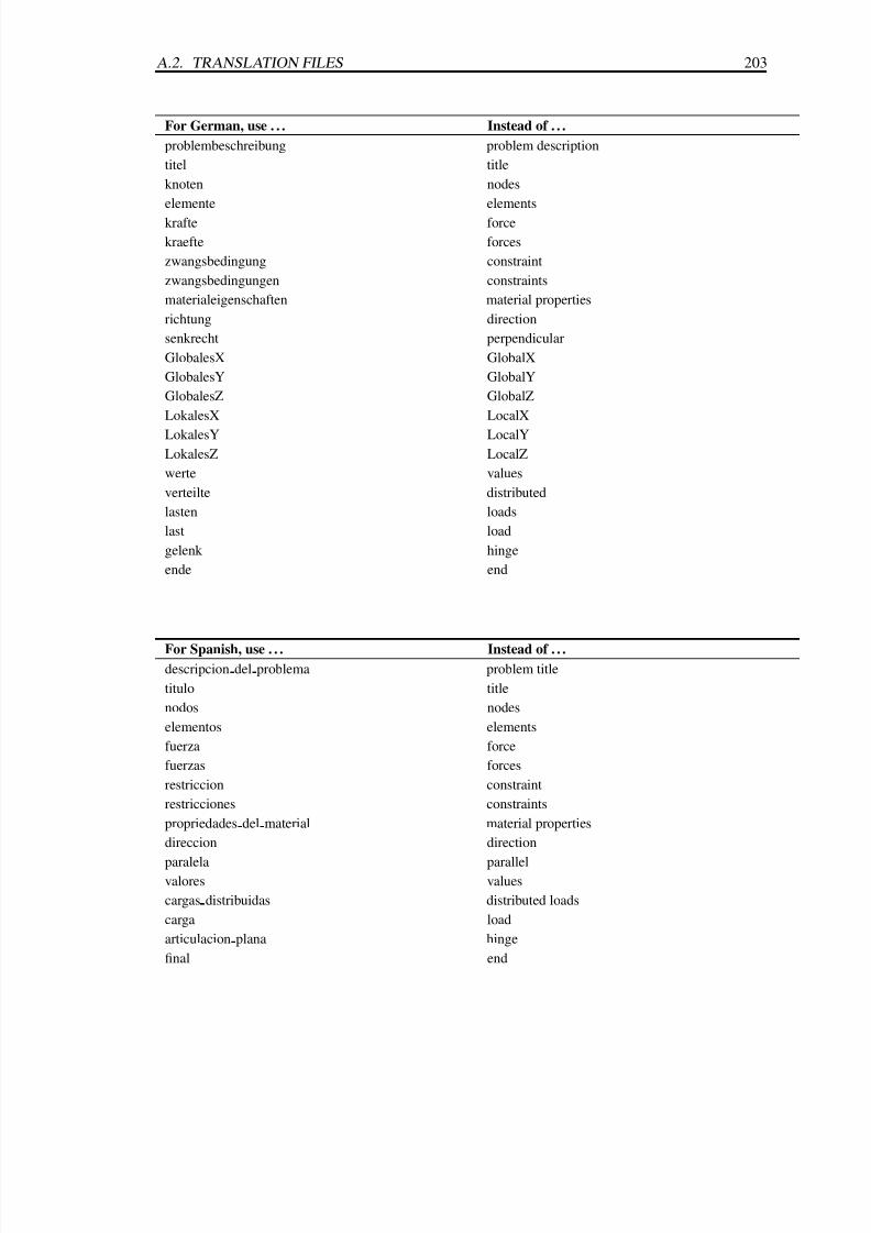
7/30/2019 Felt Manual
http://slidepdf.com/reader/full/felt-manual 225/236
A.2. TRANSLATION FILES 203
For German, use . . . Instead of . . .
problembeschreibung problem description
titel title
knoten nodes
elemente elements
krafte force
kraefte forces
zwangsbedingung constraint
zwangsbedingungen constraints
materialeigenschaften material properties
richtung direction
senkrecht perpendicular
GlobalesX GlobalX
GlobalesY GlobalY
GlobalesZ GlobalZ
LokalesX LocalX
LokalesY LocalY
LokalesZ LocalZ
werte values
verteilte distributed
lasten loads
last load
gelenk hinge
ende end
For Spanish, use . . . Instead of . . .descripcion del problema problem title
titulo title
nodos nodes
elementos elements
fuerza force
fuerzas forces
restriccion constraint
restricciones constraints
propriedades del material material properties
direccion direction
paralela parallelvalores values
cargas distribuidas distributed loads
carga load
articulacion plana hinge
final end

7/30/2019 Felt Manual
http://slidepdf.com/reader/full/felt-manual 226/236
204 APPENDIX A. INSTALLING AND ADMINISTERING FELT
A.3 Defaults and material databases
Though the defaults files and material databases are not a necessity for velvet , they are
convenient and it might be desirable to install them in a location where all users have easy
access to them, probably the same library directory as the translation files. These files too
are really nothing more than include files which can be included as a convenience for the
user.

7/30/2019 Felt Manual
http://slidepdf.com/reader/full/felt-manual 227/236
Appendix B
The GNU General Public License
Printed below is the GNU General Public License (the GPL or copyleft ), under which
FElt is licensed. It is reproduced here to clear up some of the confusion about FElt’s
copyright status—FElt is not shareware, and it is not in the public domain. The FElt system
is copyright c1993–1995 by Jason Gobat and Darren Atkinson. Thus, FElt is copyrighted,
however, you may redistribute it under the terms of the GPL printed below.
GNU GENERAL PUBLIC LICENSE
Version 2, June 1991
Copyright (C) 1989, 1991 Free Software Foundation, Inc. 675 Mass Ave, Cambridge,
MA 02139, USA Everyone is permitted to copy and distribute verbatim copies of this
license document, but changing it is not allowed.
B.1 Preamble
The licenses for most software are designed to take away your freedom to share and change
it. By contrast, the GNU General Public License is intended to guarantee your freedom to
share and change free software–to make sure the software is free for all its users. This Gen-
eral Public License applies to most of the Free Software Foundation’s software and to any
other program whose authors commit to using it. (Some other Free Software Foundation
software is covered by the GNU Library General Public License instead.) You can apply itto your programs, too.
When we speak of free software, we are referring to freedom, not price. Our General
Public Licenses are designed to make sure that you have the freedom to distribute copies
of free software (and charge for this service if you wish), that you receive source code or
205

7/30/2019 Felt Manual
http://slidepdf.com/reader/full/felt-manual 228/236
206 APPENDIX B. THE GNU GENERAL PUBLIC LICENSE
can get it if you want it, that you can change the software or use pieces of it in new free
programs; and that you know you can do these things.
To protect your rights, we need to make restrictions that forbid anyone to deny you
these rights or to ask you to surrender the rights. These restrictions translate to certain
responsibilities for you if you distribute copies of the software, or if you modify it.
For example, if you distribute copies of such a program, whether gratis or for a fee, you
must give the recipients all the rights that you have. You must make sure that they, too,
receive or can get the source code. And you must show them these terms so they know
their rights.
We protect your rights with two steps: (1) copyright the software, and (2) offer you this
license which gives you legal permission to copy, distribute and/or modify the software.
Also, for each author’s protection and ours, we want to make certain that everyone
understands that there is no warranty for this free software. If the software is modified bysomeone else and passed on, we want its recipients to know that what they have is not the
original, so that any problems introduced by others will not reflect on the original authors’
reputations.
Finally, any free program is threatened constantly by software patents. We wish to avoid
the danger that redistributors of a free program will individually obtain patent licenses, in
effect making the program proprietary. To prevent this, we have made it clear that any
patent must be licensed for everyone’s free use or not licensed at all.
The precise terms and conditions for copying, distribution and modification follow.
B.2 Terms and Conditions for Copying, Distribution, and Modifica-
tion
0. This License applies to any program or other work which contains a notice placed
by the copyright holder saying it may be distributed under the terms of this General
Public License. The “Program”, below, refers to any such program or work, and a
“work based on the Program” means either the Program or any derivative work under
copyright law: that is to say, a work containing the Program or a portion of it, eitherverbatim or with modifications and/or translated into another language. (Hereinafter,
translation is included without limitation in the term “modification”.) Each licensee
is addressed as “you”.
Activities other than copying, distribution and modification are not covered by this

7/30/2019 Felt Manual
http://slidepdf.com/reader/full/felt-manual 229/236
B.2. TERMS AND CONDITIONS 207
License; they are outside its scope. The act of running the Program is not restricted,
and the output from the Program is covered only if its contents constitute a work
based on the Program (independent of having been made by running the Program).
Whether that is true depends on what the Program does.
1. You may copy and distribute verbatim copies of the Program’s source code as you
receive it, in any medium, provided that you conspicuously and appropriately publish
on each copy an appropriate copyright notice and disclaimer of warranty; keep intact
all the notices that refer to this License and to the absence of any warranty; and give
any other recipients of the Program a copy of this License along with the Program.
You may charge a fee for the physical act of transferring a copy, and you may at your
option offer warranty protection in exchange for a fee.
2. You may modify your copy or copies of the Program or any portion of it, thus forming
a work based on the Program, and copy and distribute such modifications or work un-der the terms of Section 1 above, provided that you also meet all of these conditions:
a. You must cause the modified files to carry prominent notices stating that you
changed the files and the date of any change.
b. You must cause any work that you distribute or publish, that in whole or in part
contains or is derived from the Program or any part thereof, to be licensed as a
whole at no charge to all third parties under the terms of this License.
c. If the modified program normally reads commands interactively when run, you
must cause it, when started running for such interactive use in the most ordinary
way, to print or display an announcement including an appropriate copyright
notice and a notice that there is no warranty (or else, saying that you provide a
warranty) and that users may redistribute the program under these conditions,
and telling the user how to view a copy of this License. (Exception: if the
Program itself is interactive but does not normally print such an announcement,
your work based on the Program is not required to print an announcement.)
These requirements apply to the modified work as a whole. If identifiable sections
of that work are not derived from the Program, and can be reasonably considered
independent and separate works in themselves, then this License, and its terms, do
not apply to those sections when you distribute them as separate works. But when
you distribute the same sections as part of a whole which is a work based on the
Program, the distribution of the whole must be on the terms of this License, whose
permissions for other licensees extend to the entire whole, and thus to each and every
part regardless of who wrote it.

7/30/2019 Felt Manual
http://slidepdf.com/reader/full/felt-manual 230/236
208 APPENDIX B. THE GNU GENERAL PUBLIC LICENSE
Thus, it is not the intent of this section to claim rights or contest your rights to work
written entirely by you; rather, the intent is to exercise the right to control the distri-
bution of derivative or collective works based on the Program.
In addition, mere aggregation of another work not based on the Program with the Pro-
gram (or with a work based on the Program) on a volume of a storage or distribution
medium does not bring the other work under the scope of this License.
3. You may copy and distribute the Program (or a work based on it, under Section 2) in
object code or executable form under the terms of Sections 1 and 2 above provided
that you also do one of the following:
a. Accompany it with the complete corresponding machine-readable source code,
which must be distributed under the terms of Sections 1 and 2 above on a
medium customarily used for software interchange; or,
b. Accompany it with a written offer, valid for at least three years, to give any thirdparty, for a charge no more than your cost of physically performing source dis-
tribution, a complete machine-readable copy of the corresponding source code,
to be distributed under the terms of Sections 1 and 2 above on a medium cus-
tomarily used for software interchange; or,
c. Accompany it with the information you received as to the offer to distribute
corresponding source code. (This alternative is allowed only for noncommercial
distribution and only if you received the program in object code or executable
form with such an offer, in accord with Subsection b above.)
The source code for a work means the preferred form of the work for making mod-
ifications to it. For an executable work, complete source code means all the source
code for all modules it contains, plus any associated interface definition files, plus
the scripts used to control compilation and installation of the executable. However,
as a special exception, the source code distributed need not include anything that is
normally distributed (in either source or binary form) with the major components
(compiler, kernel, and so on) of the operating system on which the executable runs,
unless that component itself accompanies the executable.
If distribution of executable or object code is made by offering access to copy from
a designated place, then offering equivalent access to copy the source code from thesame place counts as distribution of the source code, even though third parties are not
compelled to copy the source along with the object code.
4. You may not copy, modify, sublicense, or distribute the Program except as expressly
provided under this License. Any attempt otherwise to copy, modify, sublicense or
7/30/2019 Felt Manual
http://slidepdf.com/reader/full/felt-manual 231/236
B.2. TERMS AND CONDITIONS 209
distribute the Program is void, and will automatically terminate your rights under this
License. However, parties who have received copies, or rights, from you under this
License will not have their licenses terminated so long as such parties remain in full
compliance.
5. You are not required to accept this License, since you have not signed it. However,
nothing else grants you permission to modify or distribute the Program or its deriva-
tive works. These actions are prohibited by law if you do not accept this License.
Therefore, by modifying or distributing the Program (or any work based on the Pro-
gram), you indicate your acceptance of this License to do so, and all its terms and
conditions for copying, distributing or modifying the Program or works based on it.
6. Each time you redistribute the Program (or any work based on the Program), the
recipient automatically receives a license from the original licensor to copy, distribute
or modify the Program subject to these terms and conditions. You may not impose
any further restrictions on the recipients’ exercise of the rights granted herein. You
are not responsible for enforcing compliance by third parties to this License.
7. If, as a consequence of a court judgment or allegation of patent infringement or
for any other reason (not limited to patent issues), conditions are imposed on you
(whether by court order, agreement or otherwise) that contradict the conditions of
this License, they do not excuse you from the conditions of this License. If you
cannot distribute so as to satisfy simultaneously your obligations under this License
and any other pertinent obligations, then as a consequence you may not distribute the
Program at all. For example, if a patent license would not permit royalty-free redis-
tribution of the Program by all those who receive copies directly or indirectly through
you, then the only way you could satisfy both it and this License would be to refrain
entirely from distribution of the Program.
If any portion of this section is held invalid or unenforceable under any particular
circumstance, the balance of the section is intended to apply and the section as a
whole is intended to apply in other circumstances.
It is not the purpose of this section to induce you to infringe any patents or other prop-
erty right claims or to contest validity of any such claims; this section has the sole
purpose of protecting the integrity of the free software distribution system, which is
implemented by public license practices. Many people have made generous contri-
butions to the wide range of software distributed through that system in reliance on
consistent application of that system; it is up to the author/donor to decide if he or
she is willing to distribute software through any other system and a licensee cannot
impose that choice.

7/30/2019 Felt Manual
http://slidepdf.com/reader/full/felt-manual 232/236
210 APPENDIX B. THE GNU GENERAL PUBLIC LICENSE
This section is intended to make thoroughly clear what is believed to be a conse-
quence of the rest of this License.
8. If the distribution and/or use of the Program is restricted in certain countries either
by patents or by copyrighted interfaces, the original copyright holder who places the
Program under this License may add an explicit geographical distribution limitation
excluding those countries, so that distribution is permitted only in or among countries
not thus excluded. In such case, this License incorporates the limitation as if written
in the body of this License.
9. The Free Software Foundation may publish revised and/or new versions of the Gen-
eral Public License from time to time. Such new versions will be similar in spirit to
the present version, but may differ in detail to address new problems or concerns.
Each version is given a distinguishing version number. If the Program specifies a
version number of this License which applies to it and “any later version”, you havethe option of following the terms and conditions either of that version or of any later
version published by the Free Software Foundation. If the Program does not specify
a version number of this License, you may choose any version ever published by the
Free Software Foundation.
10. If you wish to incorporate parts of the Program into other free programs whose distri-
bution conditions are different, write to the author to ask for permission. For software
which is copyrighted by the Free Software Foundation, write to the Free Software
Foundation; we sometimes make exceptions for this. Our decision will be guided by
the two goals of preserving the free status of all derivatives of our free software andof promoting the sharing and reuse of software generally.
NO WARRANTY
11. BECAUSE THE PROGRAM IS LICENSED FREE OF CHARGE, THERE IS NO
WARRANTY FOR THE PROGRAM, TO THE EXTENT PERMITTED BY AP-
PLICABLE LAW. EXCEPT WHEN OTHERWISE STATED IN WRITING THE
COPYRIGHT HOLDERS AND/OR OTHER PARTIES PROVIDE THE PROGRAM
“AS IS” WITHOUT WARRANTY OF ANY KIND, EITHER EXPRESSED OR IM-
PLIED, INCLUDING, BUT NOT LIMITED TO, THE IMPLIED WARRANTIES
OF MERCHANTABILITY AND FITNESS FOR A PARTICULAR PURPOSE. THE
ENTIRE RISK AS TO THE QUALITY AND PERFORMANCE OF THE PRO-
GRAM IS WITH YOU. SHOULD THE PROGRAM PROVE DEFECTIVE, YOU
ASSUME THE COST OF ALL NECESSARY SERVICING, REPAIR OR COR-
RECTION.
7/30/2019 Felt Manual
http://slidepdf.com/reader/full/felt-manual 233/236
B.3. HOW TO APPLY THESE TERMS 211
12. IN NO EVENT UNLESS REQUIRED BY APPLICABLE LAW OR AGREED TO
IN WRITING WILL ANY COPYRIGHT HOLDER, OR ANY OTHER PARTY
WHO MAY MODIFY AND/OR REDISTRIBUTE THE PROGRAM AS PERMIT-
TED ABOVE, BE LIABLE TO YOU FOR DAMAGES, INCLUDING ANY GEN-
ERAL, SPECIAL, INCIDENTAL OR CONSEQUENTIAL DAMAGES ARISINGOUT OF THE USE OR INABILITY TO USE THE PROGRAM (INCLUDING BUT
NOT LIMITED TO LOSS OF DATA OR DATA BEING RENDERED INACCU-
RATE OR LOSSES SUSTAINED BY YOU OR THIRD PARTIES OR A FAILURE
OF THE PROGRAM TO OPERATE WITH ANY OTHER PROGRAMS), EVEN IF
SUCH HOLDER OR OTHER PARTY HAS BEEN ADVISED OF THE POSSIBIL-
ITY OF SUCH DAMAGES.
END OF TERMS AND CONDITIONS
B.3 Appendix: How to Apply These Terms to Your New Programs
If you develop a new program, and you want it to be of the greatest possible use to the pub-
lic, the best way to achieve this is to make it free software which everyone can redistribute
and change under these terms.
To do so, attach the following notices to the program. It is safest to attach them to the
start of each source file to most effectively convey the exclusion of warranty; and each file
should have at least the “copyright” line and a pointer to where the full notice is found.
one line to give the program’s name and a brief idea of what it does. Copyright
c19yy name of author This program is free software; you can redistribute it and/or modify it under the
terms of the GNU General Public License as published by the Free Software
Foundation; either version 2 of the License, or (at your option) any later version.
This program is distributed in the hope that it will be useful, but WITHOUT
ANY WARRANTY; without even the implied warranty of MERCHANTABIL-
ITY or FITNESS FOR A PARTICULAR PURPOSE. See the GNU GeneralPublic License for more details.
You should have received a copy of the GNU General Public License along with
this program; if not, write to the Free Software Foundation, Inc., 675 Mass Ave,
Cambridge, MA 02139, USA.

7/30/2019 Felt Manual
http://slidepdf.com/reader/full/felt-manual 234/236
212 APPENDIX B. THE GNU GENERAL PUBLIC LICENSE
Also add information on how to contact you by electronic and paper mail.
If the program is interactive, make it output a short notice like this when it starts in an
interactive mode:
Gnomovision version 69, Copyright (C) 19yy name of author Gnomovision
comes with ABSOLUTELY NO WARRANTY; for details type ‘show w’. This
is free software, and you are welcome to redistribute it under certain
conditions; type ‘show c’ for details.
The hypothetical commands ‘show w’ and ‘show c’ should show the appropriate parts
of the General Public License. Of course, the commands you use may be called some-
thing other than ‘show w’ and ‘show c’; they could even be mouse-clicks or menu items–
whatever suits your program.
You should also get your employer (if you work as a programmer) or your school, if
any, to sign a “copyright disclaimer” for the program, if necessary. Here is a sample; alter
the names:
Yoyodyne, Inc., hereby disclaims all copyright interest in the program ‘Gnomo-
vision’ (which makes passes at compilers) written by James Hacker.
signature of Ty Coon, 1 April 1989 Ty Coon, President of Vice
This General Public License does not permit incorporating your program into propri-
etary programs. If your program is a subroutine library, you may consider it more useful to
permit linking proprietary applications with the library. If this is what you want to do, use
the GNU Library General Public License instead of this License.
7/30/2019 Felt Manual
http://slidepdf.com/reader/full/felt-manual 235/236
References
[1] David S. Burnett. Finite Element Analysis: From Concepts to Applications. Addison-
Wesley, Reading, MA, 1987.
[2] G.R. Cowper. The shear coefficient in Timoshenko’s beam theory. ASME Journal of
Applied Mechanics, 33:335–340, 1966.
[3] E. Cuthill and J. McKee. Reducing the bandwidth of sparse symmetric matrices. In
Proceedings of the 24th National Conference of the ACM , ACM Publ P-69, pages
157–172, New York, 1969. Association for Computing Machinery.
[4] Z. Friedman and John B. Kosmatka. An improved two-node Timoshenko beam finite
element. Computers and Structures, 47:473–481, 1993.
[5] J.A. George. Computer implementation of the finite element method. Technical Re-
port Tech. Rep. STAN-CS-71-208, Computer Science Department, Stanford Univer-
sity, Stanford, CA, 1971.
[6] Norman E. Gibbs. A hybrid profile reduction algorithm. Assoc. for Computing Ma-
chinery Trans. on Math. Software, 2:378–387, 1976.
[7] Norman E. Gibbs, William G. Poole, and Paul K. Stockmeyer. An algorithm for
reducing the bandwidth and profile of a sparse matrix. SIAM Journal of Numerical
Analysis, 13:236–249, 1976.
[8] Ernest Hinton and D. R. J. Owen. Finite Element Programming. Academic Press,
1977.
[9] Thomas J. R. Hughes. The Finite Element Method: Linear Static and Dynamic Finite Element Analysis. Prentice-Hall, Englewood Cliffs, NJ, 1987.
[10] Thomas J.R. Hughes, Robert L. Taylor, and Worsak Kanoknukulchai. A simple and
efficient finite element for plate bending. International Journal for Numerical Meth-
ods in Enginerring, 11:1529–1543, 1977.
213

7/30/2019 Felt Manual
http://slidepdf.com/reader/full/felt-manual 236/236
214 REFERENCES
[11] Barry Joe and R. B. Simpson. Triangular meshes for regions of complicated shape.
International Journal for Numerical Methods in Enginerring, 23:751–778, 1986.
[12] Brian W. Kernhigan and Dennis M. Ritchie. The C Programming Language. Prentice-
Hall, Englewood Cliffs, second edition, 1989.
[13] Daryl L. Logan. A First Course in the Finite Element Method . PWS-Kent, Boston,
second edition, 1992.
[14] Larry J Segerlind Applied Finite Element Analysis Wiley New York second edition