feedforward control: theory and applications · feedforward control: theory and applications...
TRANSCRIPT
Feedforward Control: Theory and Applications
Santosh Devasia
Mechanical Engineering Department University of Washington
Seattle, WA
Outline of talk
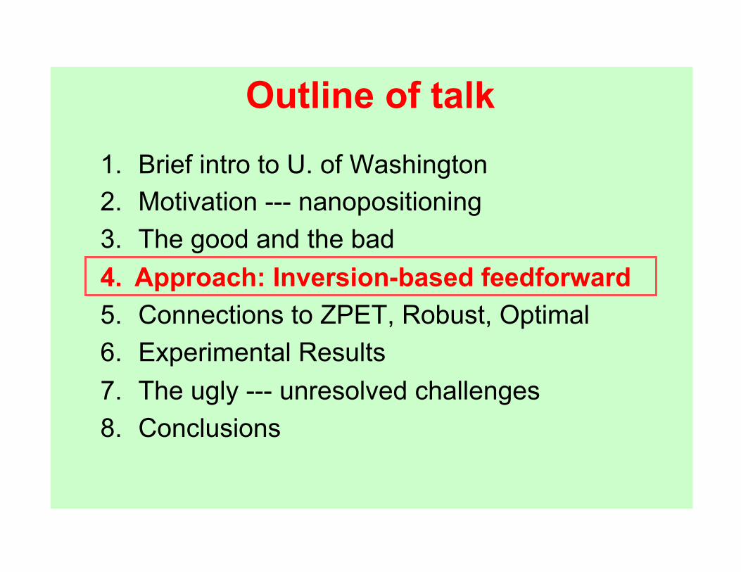
1.! Brief intro to U. of Washington 2.! Motivation --- nanopositioning 3.! The good and the bad 4.! Approach: Inversion-based feedforward 5.! Connections to ZPET, Robust, Optimal 6.! Experimental Results 7.! The ugly --- unresolved challenges 8.! Conclusions
Santosh Devasia, U. of Washington
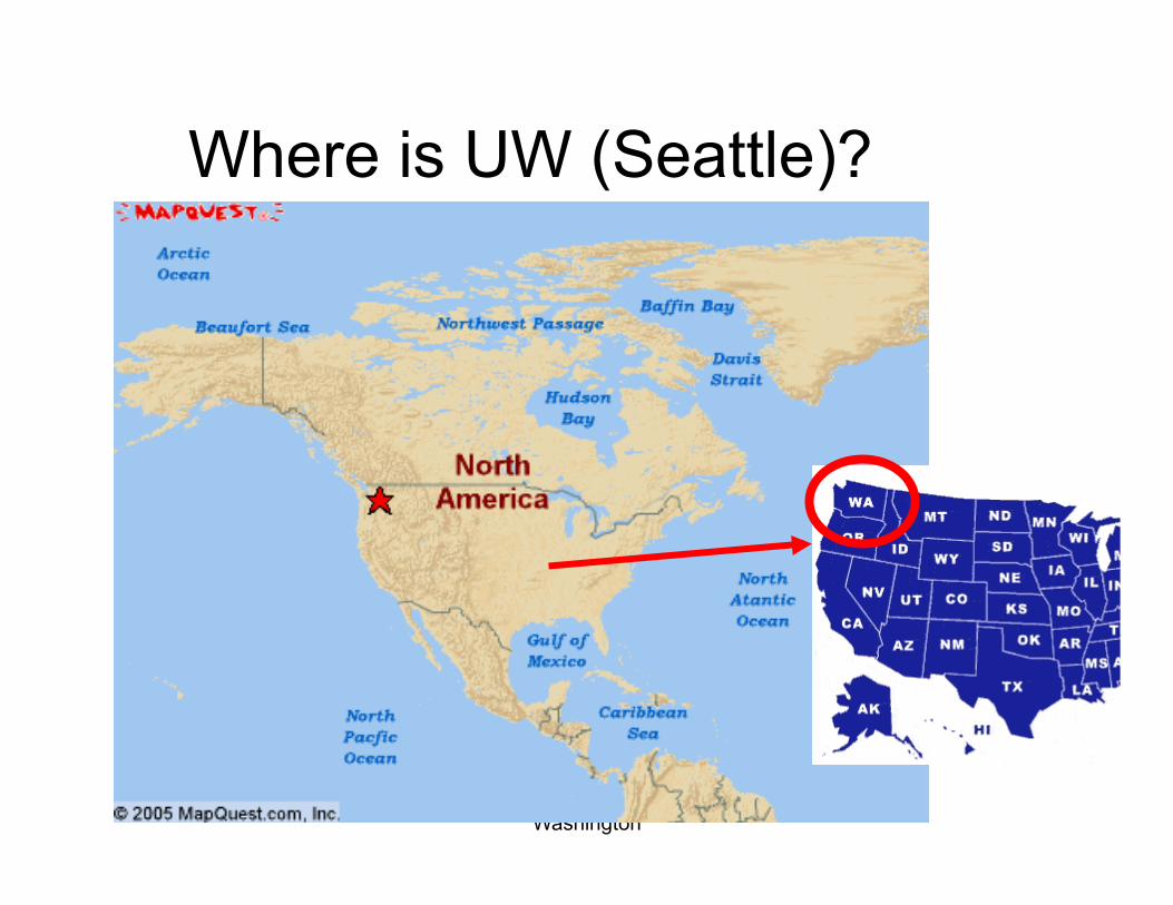
Where is UW (Seattle)?

Seattle is very Scenic
Picture by Szu-Chi Tien

Local Industries
Boeing Commercial Aircraft Division (www.boeing.com) Microsoft (www.microsoft.com) Amazon.com (www.amazon.com) Starbucks (www.starbucks.com) COSTCO, APPLES, UPS (1907) and UW

University of Washington at a Glance
•! Founded in 1861 •! 49,000 students (fall of 2010) •! Faculty of nearly 4,000 includes:
– Six Nobel Prize winners •! Research budget (2010)
more than US $ 1 billion •! Ranked in top 20 of world universities
(16th) http://www.arwu.org
•! Overall --- a nice to work
•! …and a nice place to visit !!
ravian100.wordpress.com
pcbsmi.org
Outline of talk
1.! Brief intro to U. of Washington 2.! Motivation --- nanopositioning 3.! The good and the bad 4.! Approach: Inversion-based feedforward 5.! Connections to ZPET, Robust, Optimal 6.! Experimental Results 7.! The ugly --- unresolved challenges 8.! Conclusions
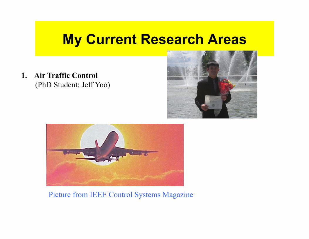
My Current Research Areas
Picture from IEEE Control Systems Magazine
1.! Air Traffic Control
(PhD Student: Jeff Yoo)
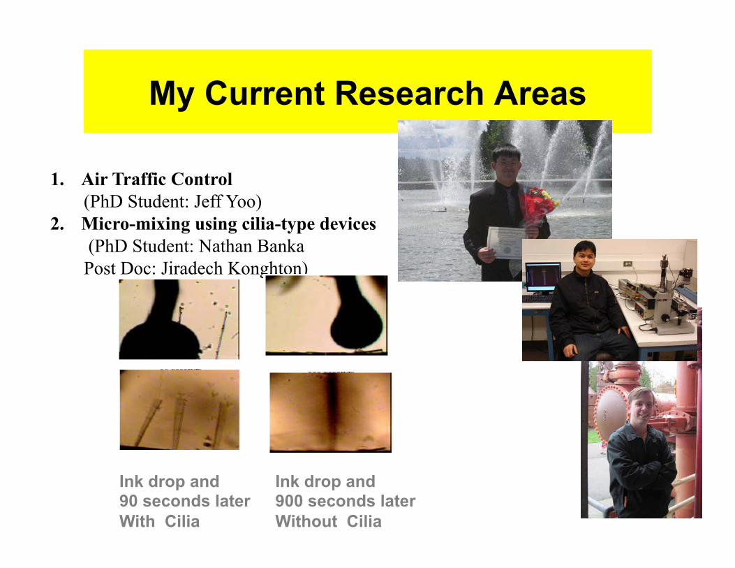
My Current Research Areas
1.! Air Traffic Control
(PhD Student: Jeff Yoo) 2.! Micro-mixing using cilia-type devices
(PhD Student: Nathan Banka Post Doc: Jiradech Konghton)
Ink drop and 90 seconds later With Cilia
Ink drop and 900 seconds later Without Cilia
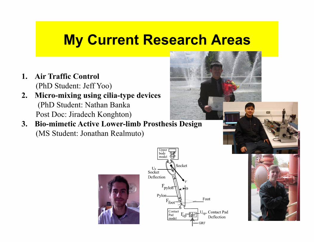
My Current Research Areas
1.! Air Traffic Control
(PhD Student: Jeff Yoo) 2.! Micro-mixing using cilia-type devices
(PhD Student: Nathan Banka Post Doc: Jiradech Konghton)
3.! Bio-mimetic Active Lower-limb Prosthesis Design (MS Student: Jonathan Realmuto)
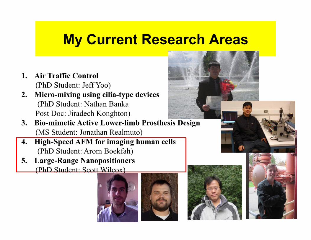
My Current Research Areas
1.! Air Traffic Control
(PhD Student: Jeff Yoo) 2.! Micro-mixing using cilia-type devices
(PhD Student: Nathan Banka Post Doc: Jiradech Konghton)
3.! Bio-mimetic Active Lower-limb Prosthesis Design (MS Student: Jonathan Realmuto)
4.! High-Speed AFM for imaging human cells (PhD Student: Arom Boekfah)
5.! Large-Range Nanopositioners (PhD Student: Scott Wilcox)
Talk based on review article in ASME
A Review of Feedforward Control Approaches in Nanopositioning for High Speed SPM ASME J. of Dyn. Sys., Meas. and Control, 131 (6), Article number 061001, pp. 1-19, Nov. 2009 PDF of talk: http://faculty.washington.edu/devasia/
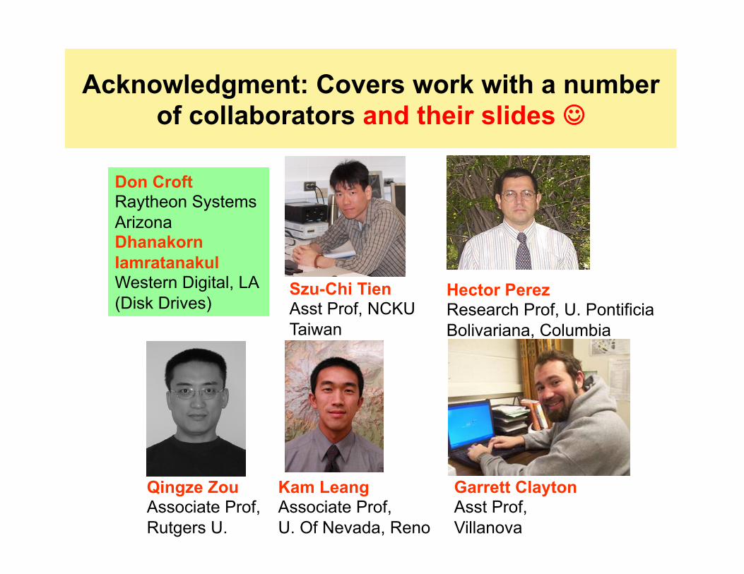
Acknowledgment: Covers work with a number of collaborators and their slides !!
Szu-Chi Tien Asst Prof, NCKU Taiwan
Hector Perez Research Prof, U. Pontificia Bolivariana, Columbia
Kam Leang Associate Prof, U. Of Nevada, Reno
Qingze Zou Associate Prof, Rutgers U.
Garrett Clayton Asst Prof, Villanova
Don Croft Raytheon Systems Arizona Dhanakorn Iamratanakul Western Digital, LA (Disk Drives)
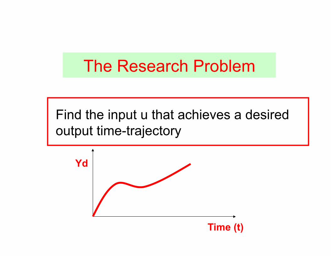
The Research Problem
Find the input u that achieves a desired output time-trajectory
Yd
Time (t)
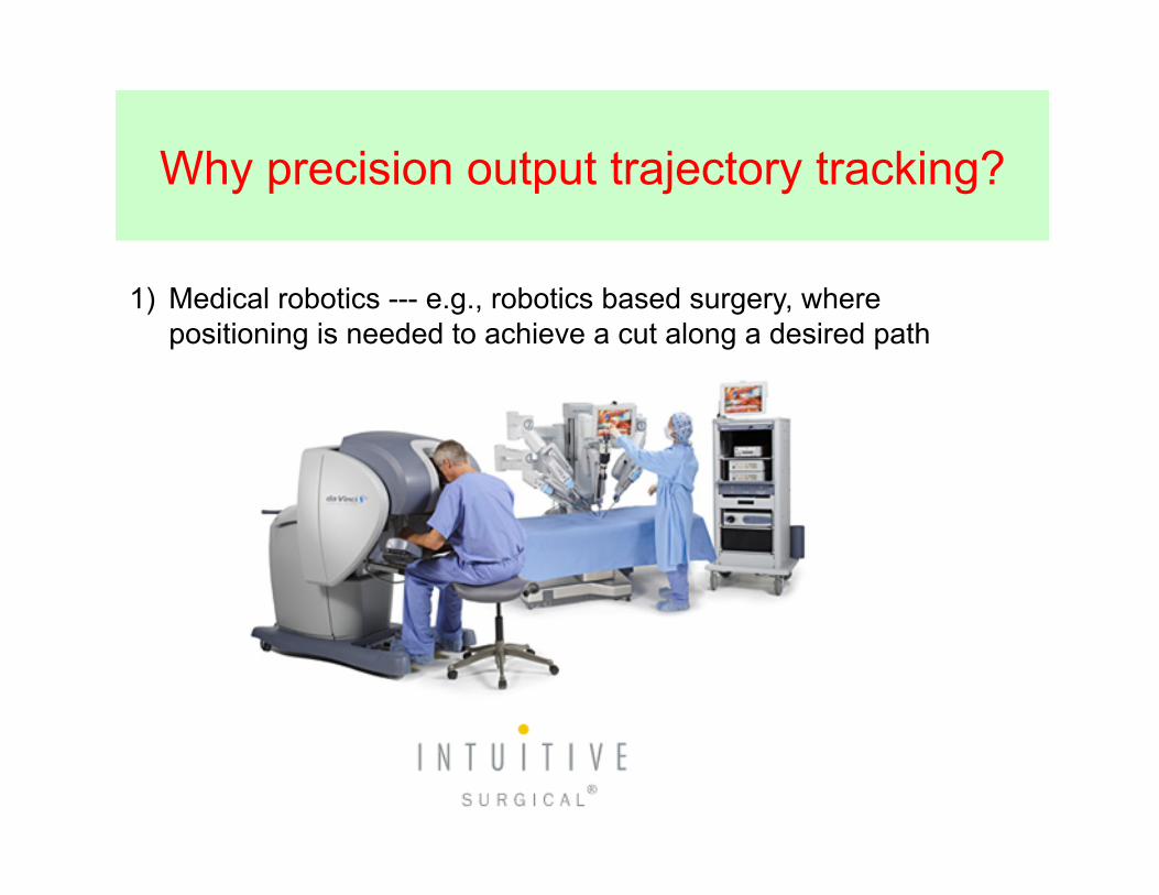
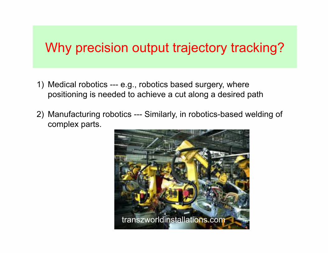
Why precision output trajectory tracking?
1)! Medical robotics --- e.g., robotics based surgery, where positioning is needed to achieve a cut along a desired path
Why precision output trajectory tracking?
1)! Medical robotics --- e.g., robotics based surgery, where positioning is needed to achieve a cut along a desired path
2)! Manufacturing robotics --- Similarly, in robotics-based welding of complex parts.
transzworldinstallations.com
Why precision output trajectory tracking?
1)! Medical robotics --- e.g., robotics based surgery, where positioning is needed to achieve a cut along a desired path
2)! Manufacturing robotics --- Similarly, in robotics-based welding of complex parts.
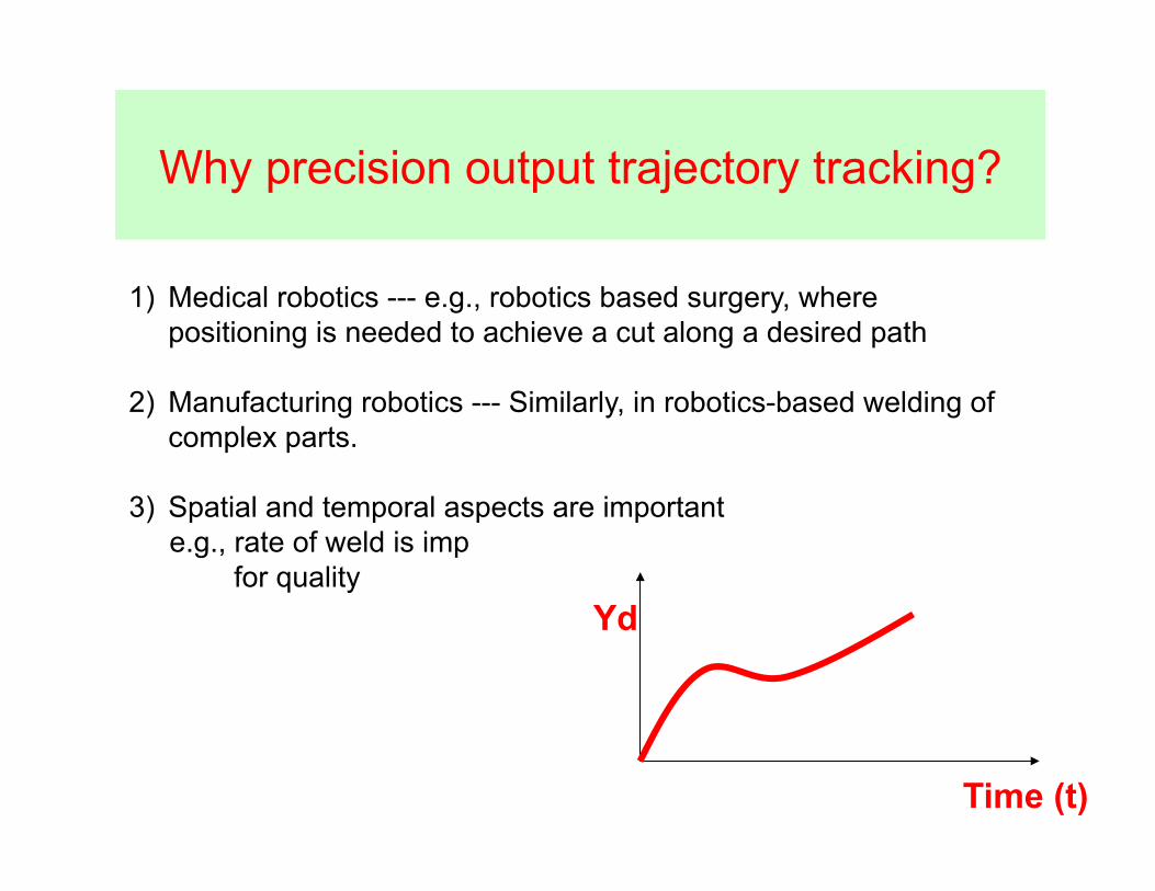
3)! Spatial and temporal aspects are important e.g., rate of weld is imp
for quality
Yd
Time (t)
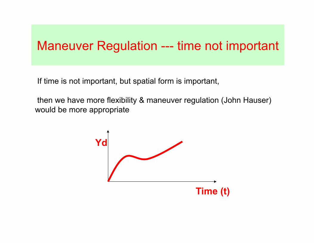
Maneuver Regulation --- time not important
If time is not important, but spatial form is important, then we have more flexibility & maneuver regulation (John Hauser) would be more appropriate
Yd
Time (t)
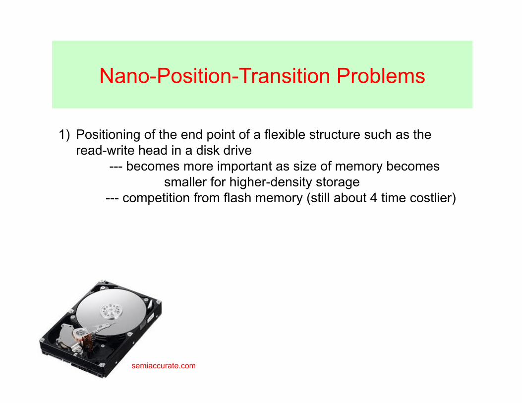
Nano-Position-Transition Problems
1)! Positioning of the end point of a flexible structure such as the read-write head in a disk drive
--- becomes more important as size of memory becomes smaller for higher-density storage --- competition from flash memory (still about 4 time costlier)
semiaccurate.com
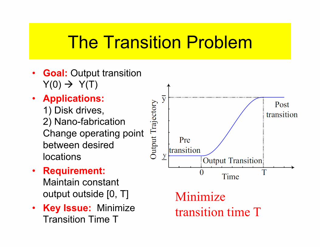
The Transition Problem •! Goal: Output transition
Y(0) " Y(T) •! Applications:
1) Disk drives, 2) Nano-fabrication Change operating point between desired locations
•! Requirement: Maintain constant output outside [0, T]
•! Key Issue: Minimize Transition Time T
Minimize transition time T

Standard State Transition SST •! Approach: Find
equilibrium states X(0) and X(T) corresponding to outputs Y(0) and Y(T)
•! Problem: Minimum time state transition X(0) " X(T)
•! Standard Solution: Bang-Bang inputs
•! No Pre- and Post-actuation: Input applied during transition time interval [0,T]
Inpu
t U
X(0) X(T)
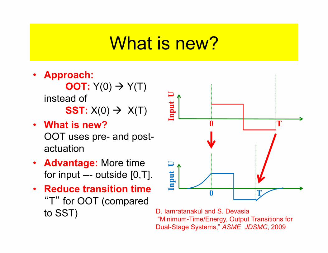
What is new? •! Approach:
OOT: Y(0) " Y(T) instead of
SST: X(0) " X(T) •! What is new?
OOT uses pre- and post- actuation
•! Advantage: More time for input --- outside [0,T].
•! Reduce transition time T for OOT (compared
to SST)
0 T
Inpu
t U
0 T
Inpu
t U
D. Iamratanakul and S. Devasia “Minimum-Time/Energy, Output Transitions for Dual-Stage Systems,” ASME JDSMC, 2009
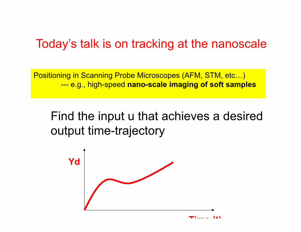
Today’s talk is on tracking at the nanoscale
Positioning in Scanning Probe Microscopes (AFM, STM, etc!) --- e.g., high-speed nano-scale imaging of soft samples
Yd
Time (t)
Find the input u that achieves a desired output time-trajectory

Example: Cell Imaging with AFM Investigate, reasons for abnormal cell behavior, e.g., due to aging or cancer, and how to correct it Similar to Doctor tapping on stomach to diagnose reason for abdominal pain AFM probe is used to tap on a human cell But with very small forces (pN) 10-12N
probe
Cell
Actuator
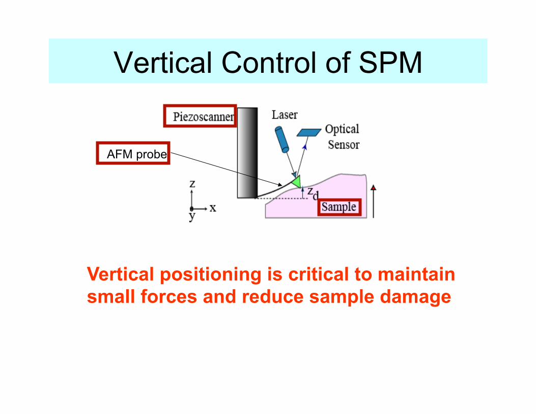
Vertical Control of SPM
Vertical positioning is critical to maintain small forces and reduce sample damage
AFM probe
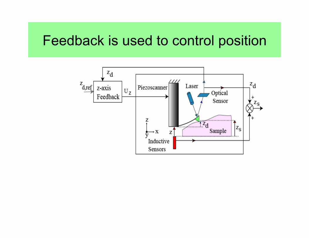
Feedback is used to control position
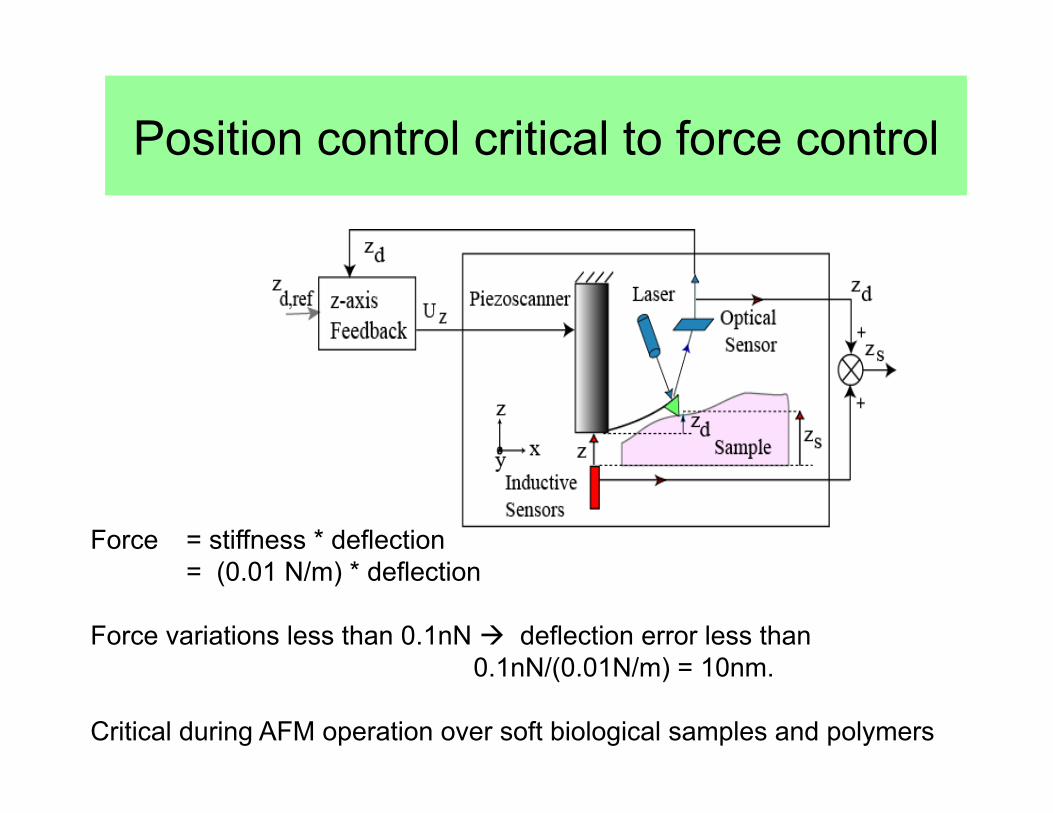
Position control critical to force control
Force = stiffness * deflection = (0.01 N/m) * deflection Force variations less than 0.1nN " deflection error less than
0.1nN/(0.01N/m) = 10nm. Critical during AFM operation over soft biological samples and polymers

AFM Imaging of soft cells is slow!
If you are slow --- a good integral controller (PID) can track with very high precision --- due to robustness of “I” But slow -- About 20 minutes … cells can change during this time
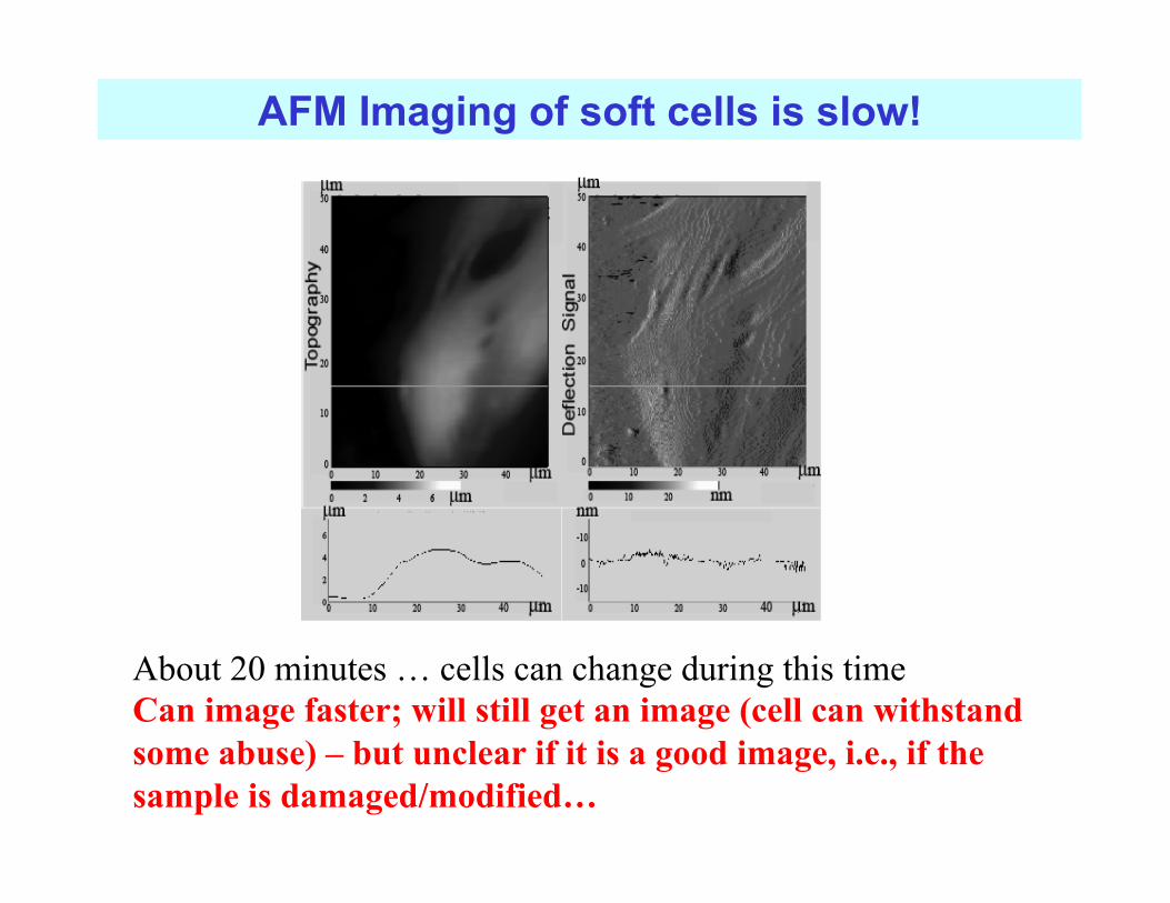
AFM Imaging of soft cells is slow!
About 20 minutes … cells can change during this time Can image faster; will still get an image (cell can withstand some abuse) – but unclear if it is a good image, i.e., if the sample is damaged/modified…

Typical goals in positioning control Find the input u that achieves the desired output (position) time-trajectory
Yd
Time (t) Goals: High-speed, high-precision, large-range
Outline of talk
1.! Brief intro to U. of Washington 2.! Motivation --- nanopositioning 3.! The good and the bad 4.! Approach: Inversion-based feedforward 5.! Connections to ZPET, Robust, Optimal 6.! Experimental Results 7.! The ugly --- unresolved challenges 8.! Conclusions

The good, the bad, and the ugly in
Nanopositioning
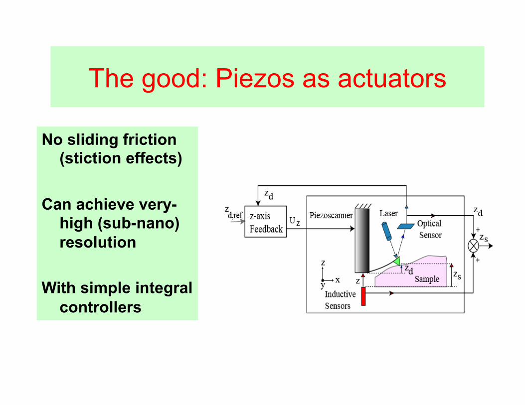
No sliding friction (stiction effects)
Can achieve very-
high (sub-nano) resolution
With simple integral
controllers
The good: Piezos as actuators

The good, the bad, and the ugly in
Nanopositioning
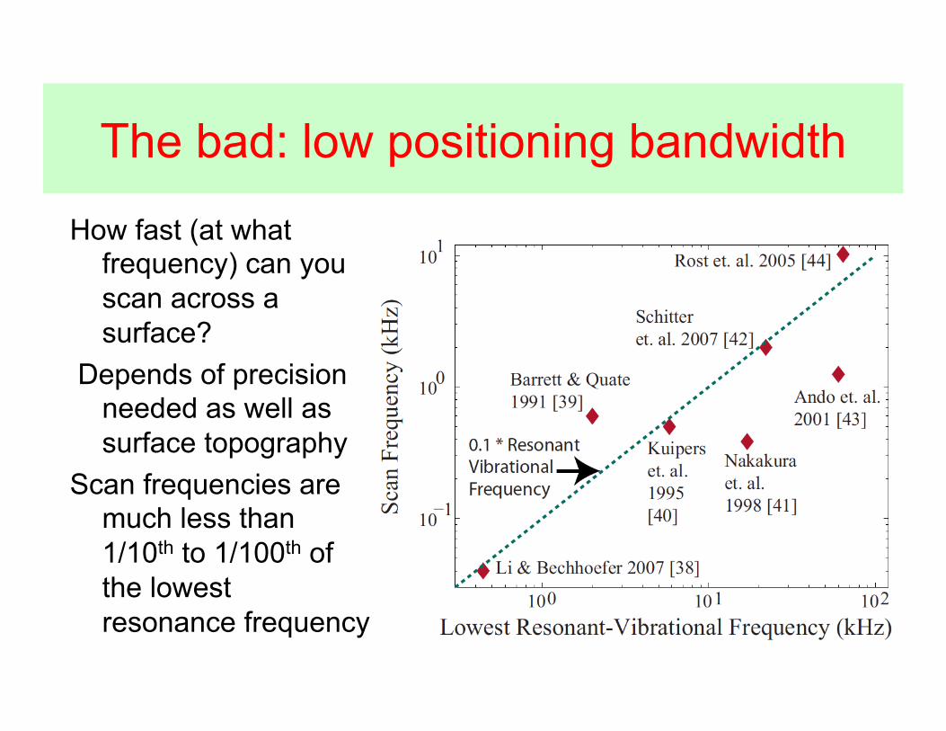
How fast (at what frequency) can you scan across a surface?
Depends of precision needed as well as surface topography
Scan frequencies are much less than 1/10th to 1/100th of the lowest resonance frequency
The bad: low positioning bandwidth
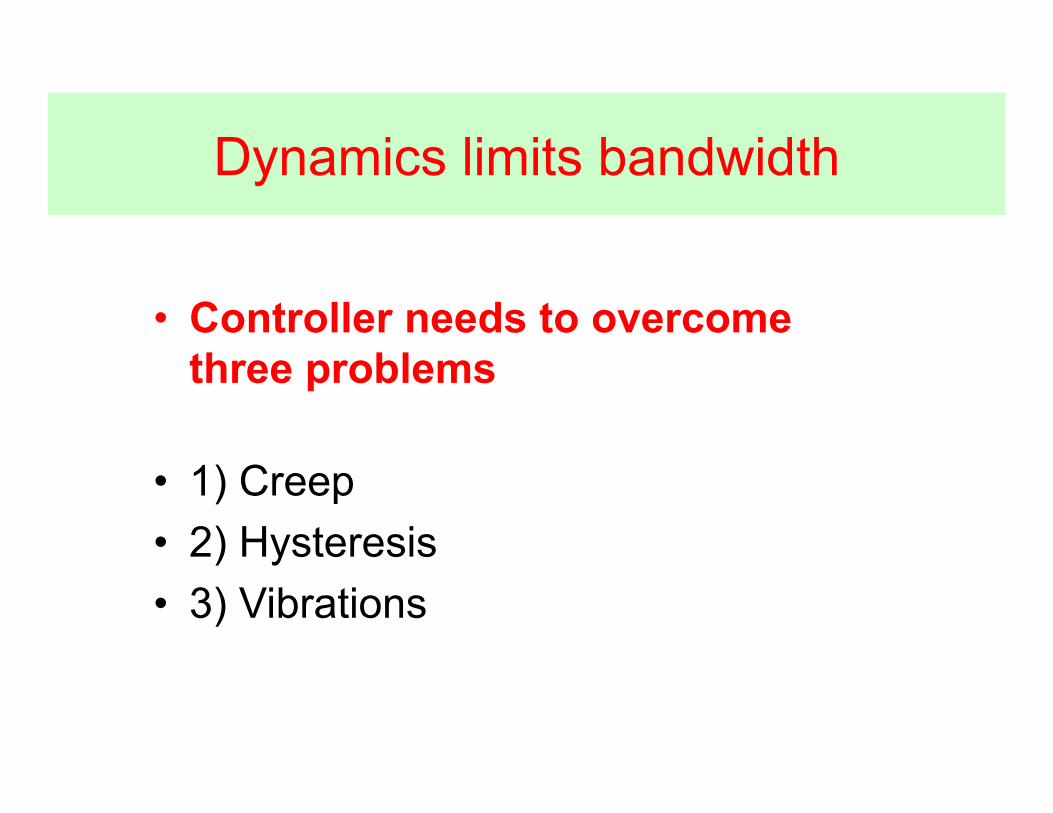
Dynamics limits bandwidth
•! Controller needs to overcome three problems
•! 1) Creep •! 2) Hysteresis •! 3) Vibrations
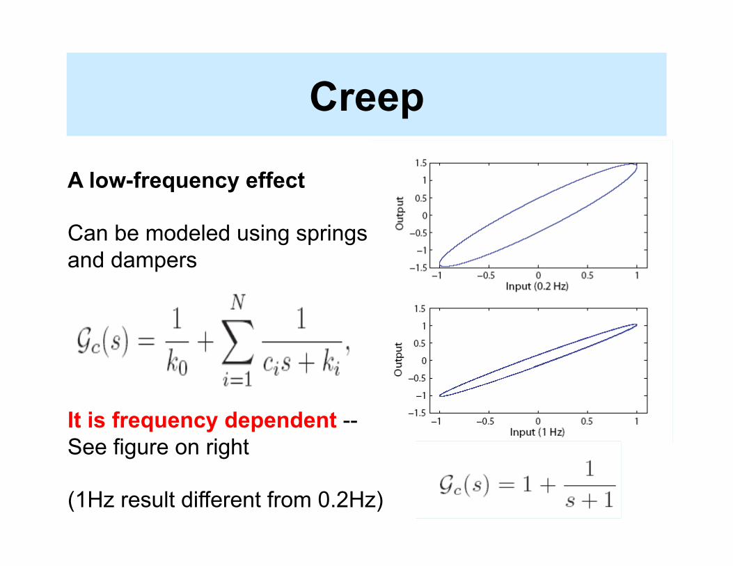
Creep
A low-frequency effect Can be modeled using springs and dampers It is frequency dependent --See figure on right (1Hz result different from 0.2Hz)
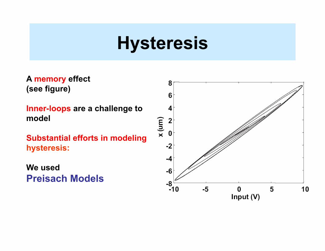
Hysteresis
A memory effect (see figure) Inner-loops are a challenge to model Substantial efforts in modeling hysteresis: We used Preisach Models
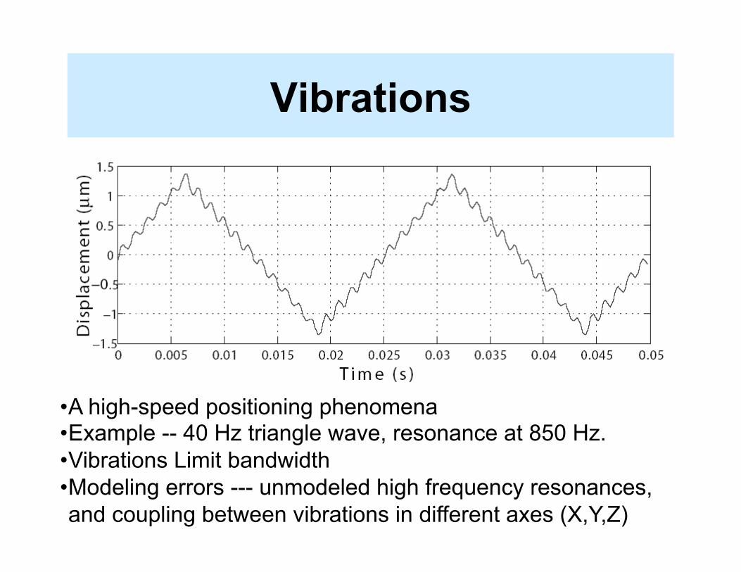
Vibrations
•!A high-speed positioning phenomena •!Example -- 40 Hz triangle wave, resonance at 850 Hz. •!Vibrations Limit bandwidth •!Modeling errors --- unmodeled high frequency resonances, and coupling between vibrations in different axes (X,Y,Z)
Outline of talk
1.! Brief intro to U. of Washington 2.! Motivation --- nanopositioning 3.! The good and the bad 4.! Approach: Inversion-based feedforward 5.! Connections to ZPET, Robust, Optimal 6.! Experimental Results 7.! The ugly --- unresolved challenges 8.! Conclusions
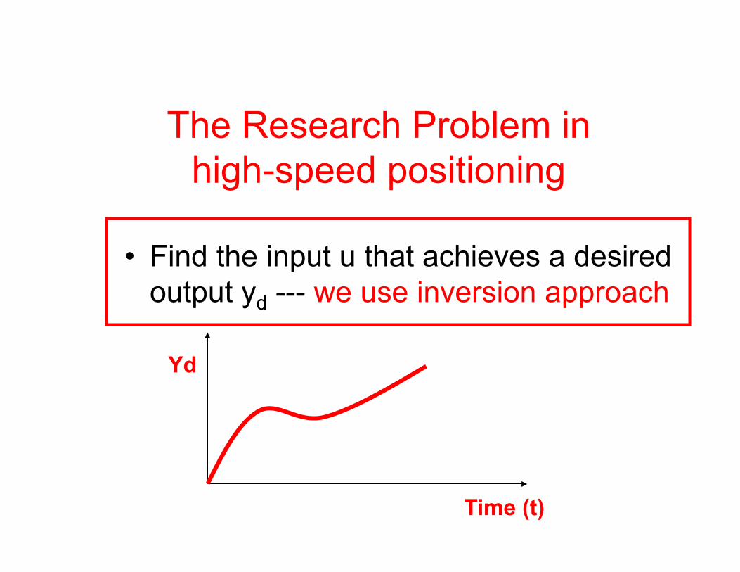
The Research Problem in high-speed positioning
•! Find the input u that achieves a desired
output yd --- we use inversion approach
Yd
Time (t)
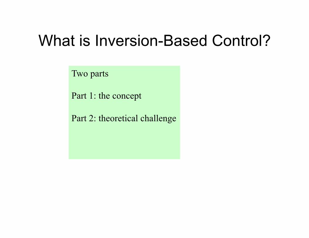
What is Inversion-Based Control?
Two parts Part 1: the concept Part 2: theoretical challenge
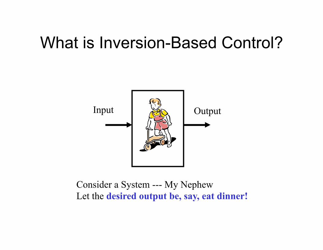
What is Inversion-Based Control?
Input Output
Consider a System --- My Nephew Let the desired output be, say, eat dinner!

What is Inversion-Based Control?
Input Output = Yd
Let the desired output be, say, eat dinner! Question: What input should you apply? (negotiate, encourage, ???)
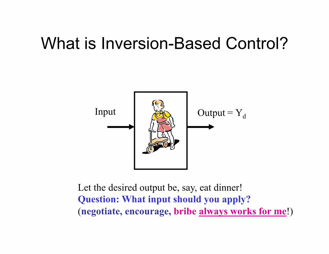
What is Inversion-Based Control?
Input Output = Yd
Let the desired output be, say, eat dinner! Question: What input should you apply? (negotiate, encourage, bribe always works for me!)
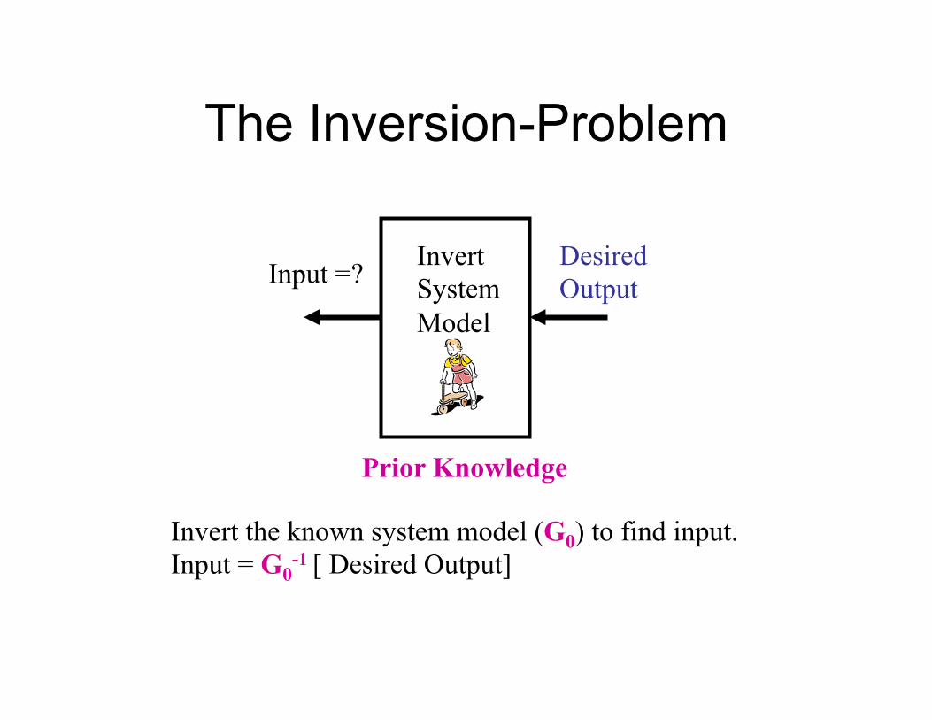
The Inversion-Problem
Input =? Desired Output
Invert the known system model (G0) to find input. Input = G0
-1 [ Desired Output]
Invert System Model
Prior Knowledge

The Inversion-Problem
Input =? Desired Output
Invert the known system model (G0) to find input. Input = G0
-1 [ Desired Output]
Invert System Model
Prior Knowledge
(His Mom know s how --- she has a reasonable model)
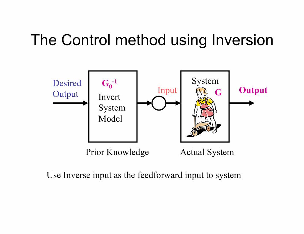
The Control method using Inversion
Use Inverse input as the feedforward input to system
Prior Knowledge Actual System
Input Output Invert System Model
Desired Output
System G0-1
G
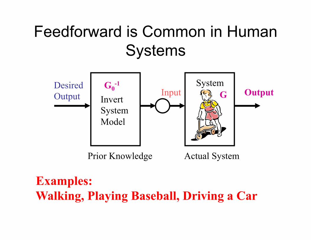
Feedforward is Common in Human Systems
Prior Knowledge Actual System
Input Output Invert System Model
Desired Output
System G0-1
G
Examples: Walking, Playing Baseball, Driving a Car
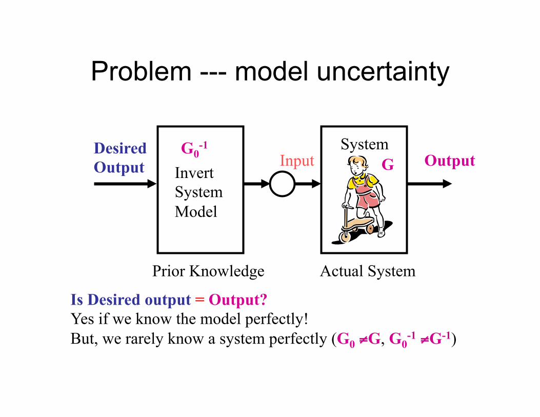
Problem --- model uncertainty
Is Desired output = Output? Yes if we know the model perfectly! But, we rarely know a system perfectly (G0 !!G, G0
-1 !!G-1)
Prior Knowledge Actual System
Input Output Invert System Model
Desired Output
System G0-1
G
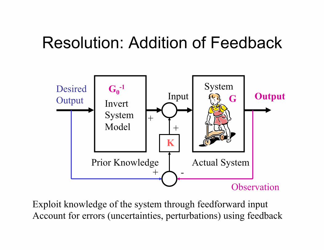
Resolution: Addition of Feedback
Exploit knowledge of the system through feedforward input Account for errors (uncertainties, perturbations) using feedback
Input Invert System Model
Desired Output
System
K
+ -
+ +
Observation
Output
Prior Knowledge Actual System
G0-1
G
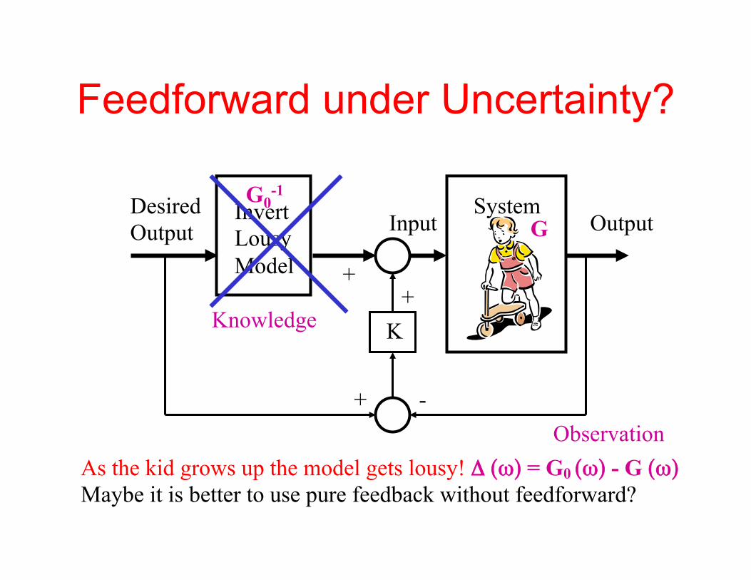
Feedforward under Uncertainty?
As the kid grows up the model gets lousy! "" ((##)) = G0 ((##)) - G ((##)) Maybe it is better to use pure feedback without feedforward?
Input Output Invert Lousy Model
Desired Output
System
K
+ -
+ +
Knowledge
Observation
G0-1
G
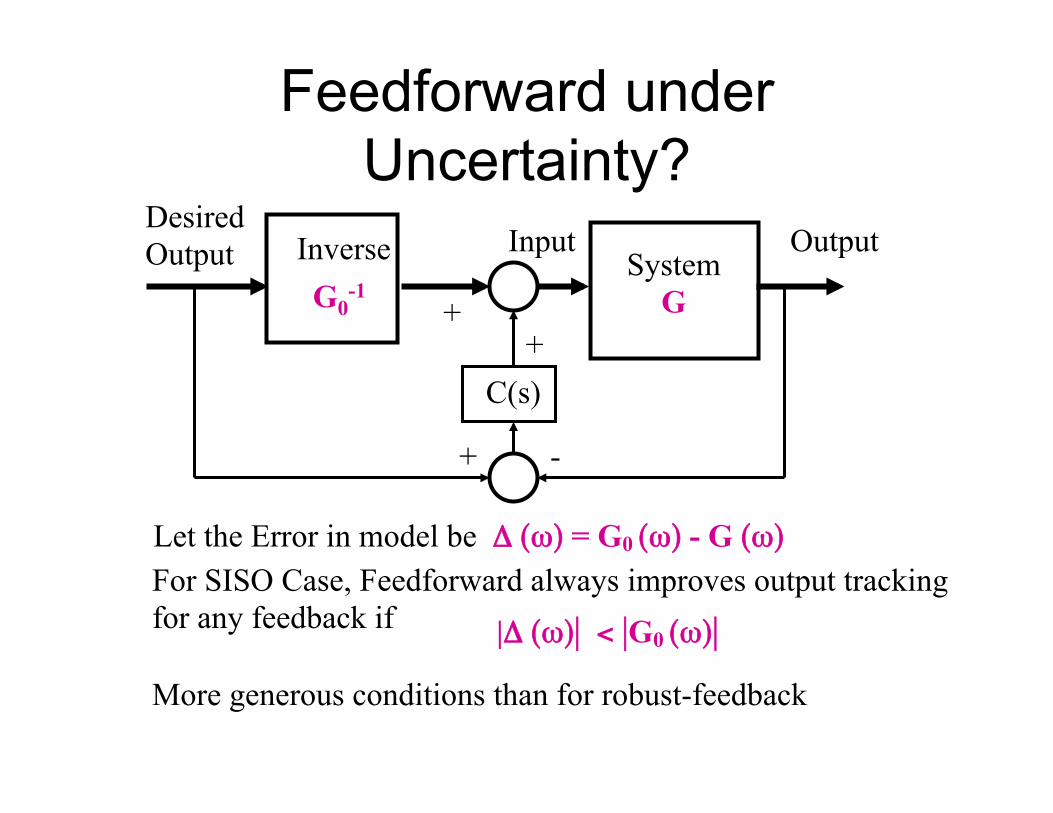
Feedforward under Uncertainty?
Input Output
G0-1
Desired Output System
G
C(s)
+ -
+ +
Inverse
Let the Error in model be "" ((##)) = G0 ((##)) - G ((##)) $$$$For SISO Case, Feedforward always improves output tracking for any feedback if More generous conditions than for robust-feedback
|"" ((##))|| << ||G0 ((##))||
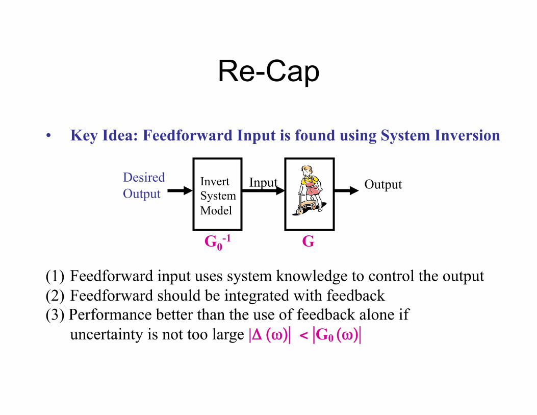
•! Key Idea: Feedforward Input is found using System Inversion
(1)! Feedforward input uses system knowledge to control the output (2)! Feedforward should be integrated with feedback (3) Performance better than the use of feedback alone if
uncertainty is not too large |"" ((##))|| << ||G0 ((##))||$$
Re-Cap
Input Output Invert System Model
Desired Output
G0-1 G

What is Inversion-Based Control?
Two parts Part 1: the concept Part 2: theoretical challenge
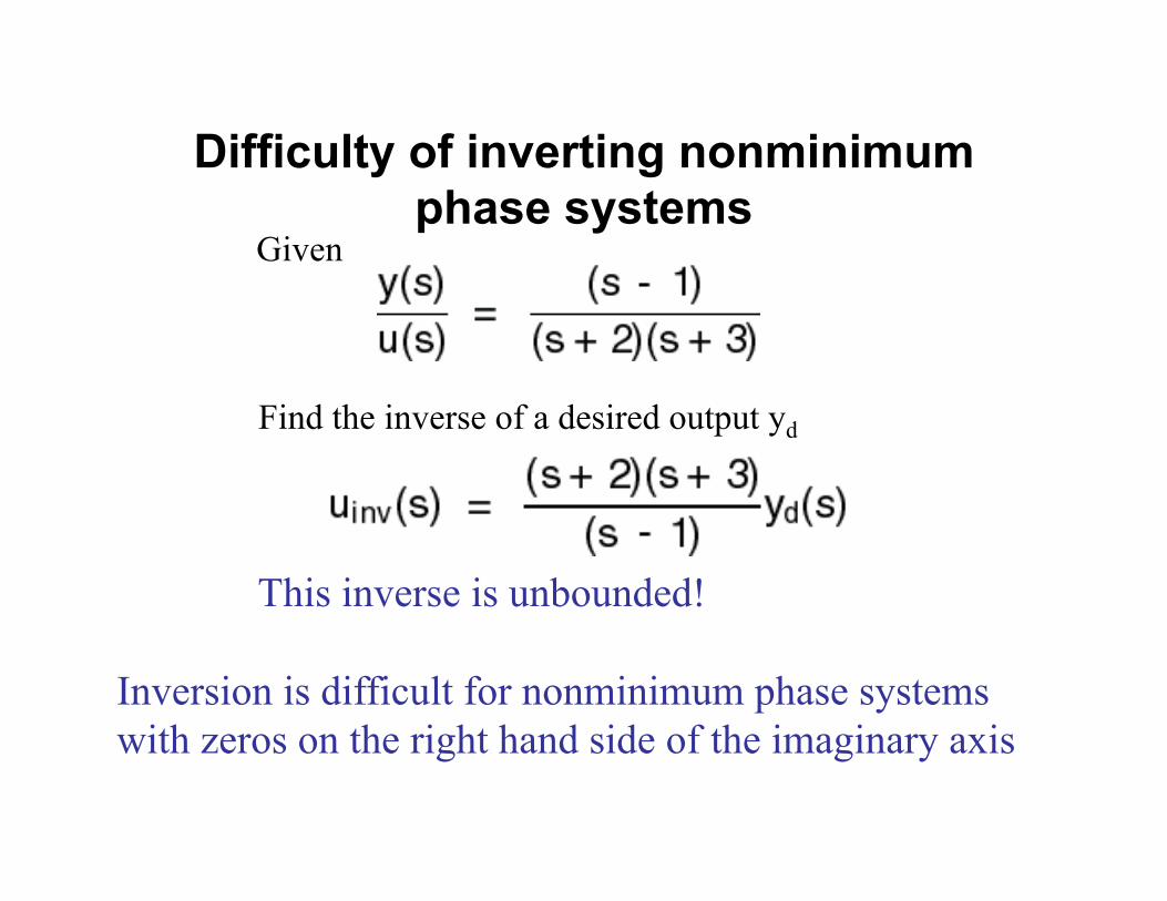
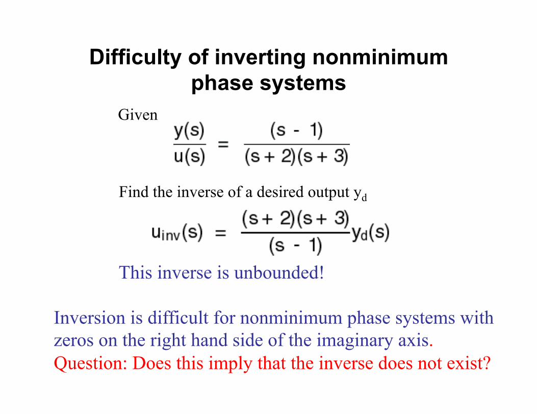
Difficulty of inverting nonminimum
phase systems
This inverse is unbounded!
Given
Find the inverse of a desired output yd
Inversion is difficult for nonminimum phase systems with zeros on the right hand side of the imaginary axis
Difficulty of inverting nonminimum phase systems
This inverse is unbounded!
Given
Find the inverse of a desired output yd
Inversion is difficult for nonminimum phase systems with zeros on the right hand side of the imaginary axis. Question: Does this imply that the inverse does not exist?
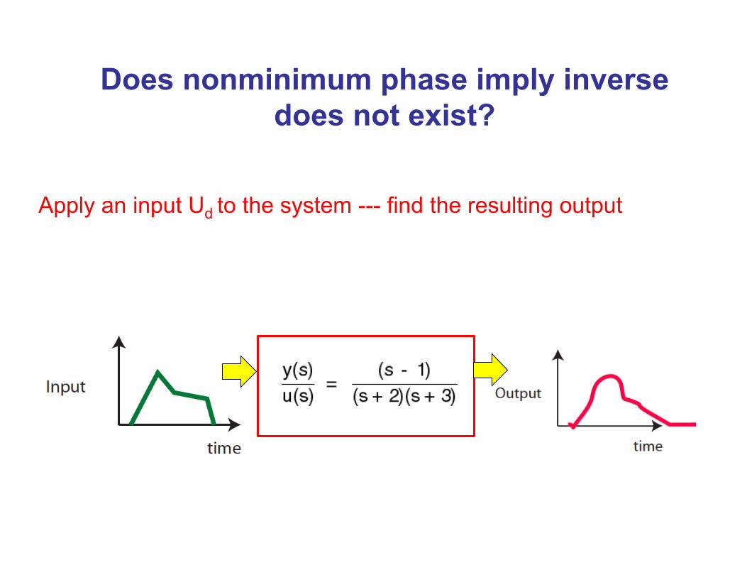
Does nonminimum phase imply inverse does not exist?
Apply an input Ud to the system --- find the resulting output

Does nonminimum phase imply inverse does not exist?
Apply an input Ud to the system --- find the resulting output
Choose this output as the desired output Yd
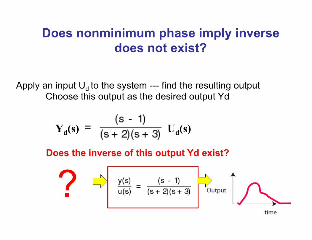
Does nonminimum phase imply inverse does not exist?
Apply an input Ud to the system --- find the resulting output
Choose this output as the desired output Yd
Does the inverse of this output Yd exist?
Yd(s) Ud(s)
?
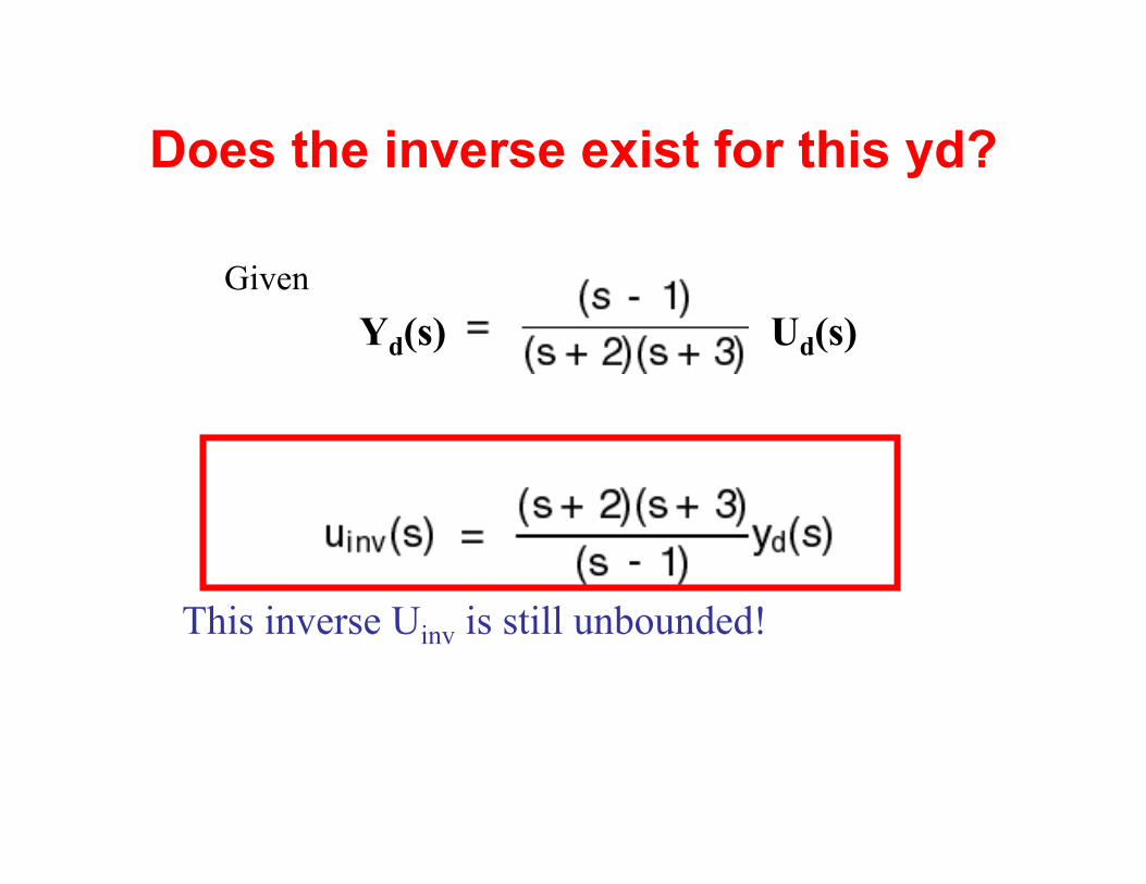
Does the inverse exist for this yd?
This inverse Uinv is still unbounded!
Given Yd(s) Ud(s)
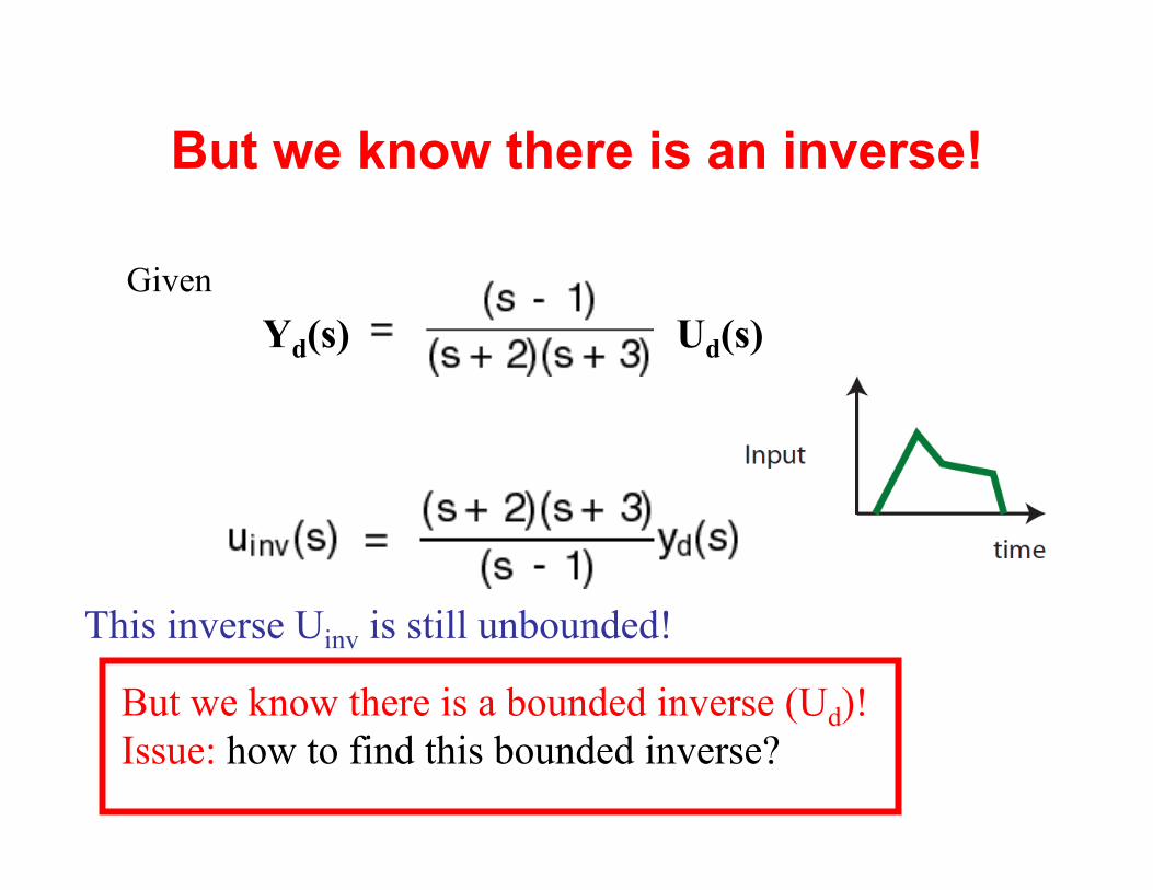
But we know there is an inverse!
This inverse Uinv is still unbounded!
Given
But we know there is a bounded inverse (Ud)! Issue: how to find this bounded inverse?
Yd(s) Ud(s)
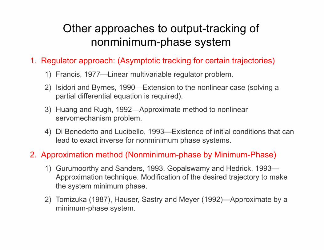
Other approaches to output-tracking of nonminimum-phase system
1.! Regulator approach: (Asymptotic tracking for certain trajectories) 1)! Francis, 1977—Linear multivariable regulator problem.
2)! Isidori and Byrnes, 1990—Extension to the nonlinear case (solving a partial differential equation is required).
3)! Huang and Rugh, 1992—Approximate method to nonlinear servomechanism problem.
4)! Di Benedetto and Lucibello, 1993—Existence of initial conditions that can lead to exact inverse for nonminimum phase systems.
2.! Approximation method (Nonminimum-phase by Minimum-Phase) 1)! Gurumoorthy and Sanders, 1993, Gopalswamy and Hedrick, 1993—
Approximation technique. Modification of the desired trajectory to make the system minimum phase.
2)! Tomizuka (1987), Hauser, Sastry and Meyer (1992)—Approximate by a minimum-phase system.
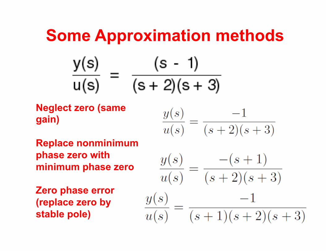
Some Approximation methods
Neglect zero (same gain) Replace nonminimum phase zero with minimum phase zero Zero phase error (replace zero by stable pole)
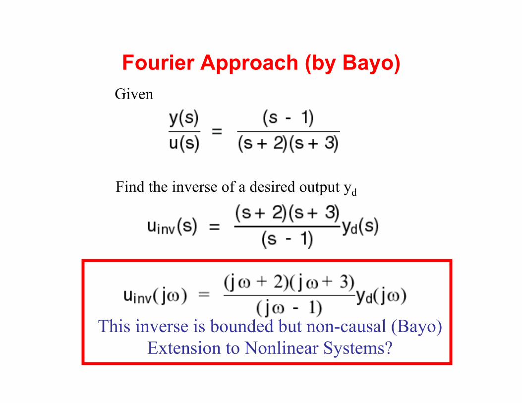
Fourier Approach (by Bayo)
This inverse is bounded but non-causal (Bayo) Extension to Nonlinear Systems?
Given
Find the inverse of a desired output yd
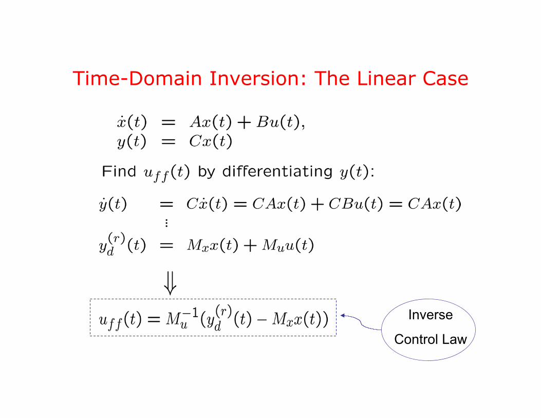
Time-Domain Inversion: The Linear Case
Inverse
Control Law

Find the inverse control law
Internal
Dynamics
Inverse
Control Law
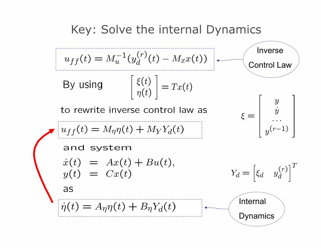
Key: Solve the internal Dynamics
Internal
Dynamics
Inverse
Control Law
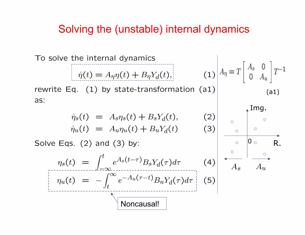
(a1)
R. 0
Img.
Solving the (unstable) internal dynamics
Noncausal!
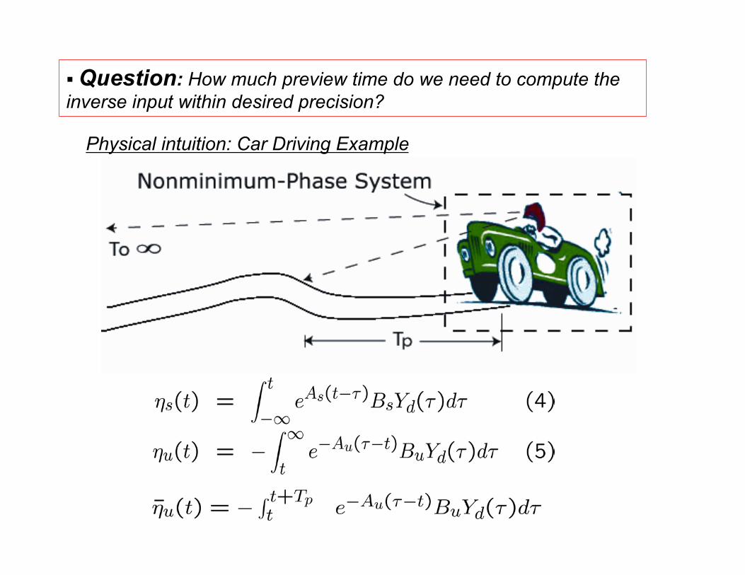
Physical intuition: Car Driving Example
#! Question: How much preview time do we need to compute the inverse input within desired precision?

#! Question: How much preview time do we need to compute the inverse input within desired precision?
Preview time:
Settling time:
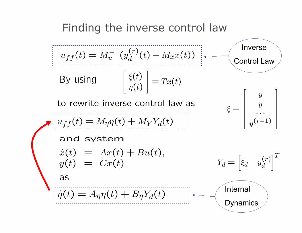
Finding the inverse control law
Internal
Dynamics
Inverse
Control Law
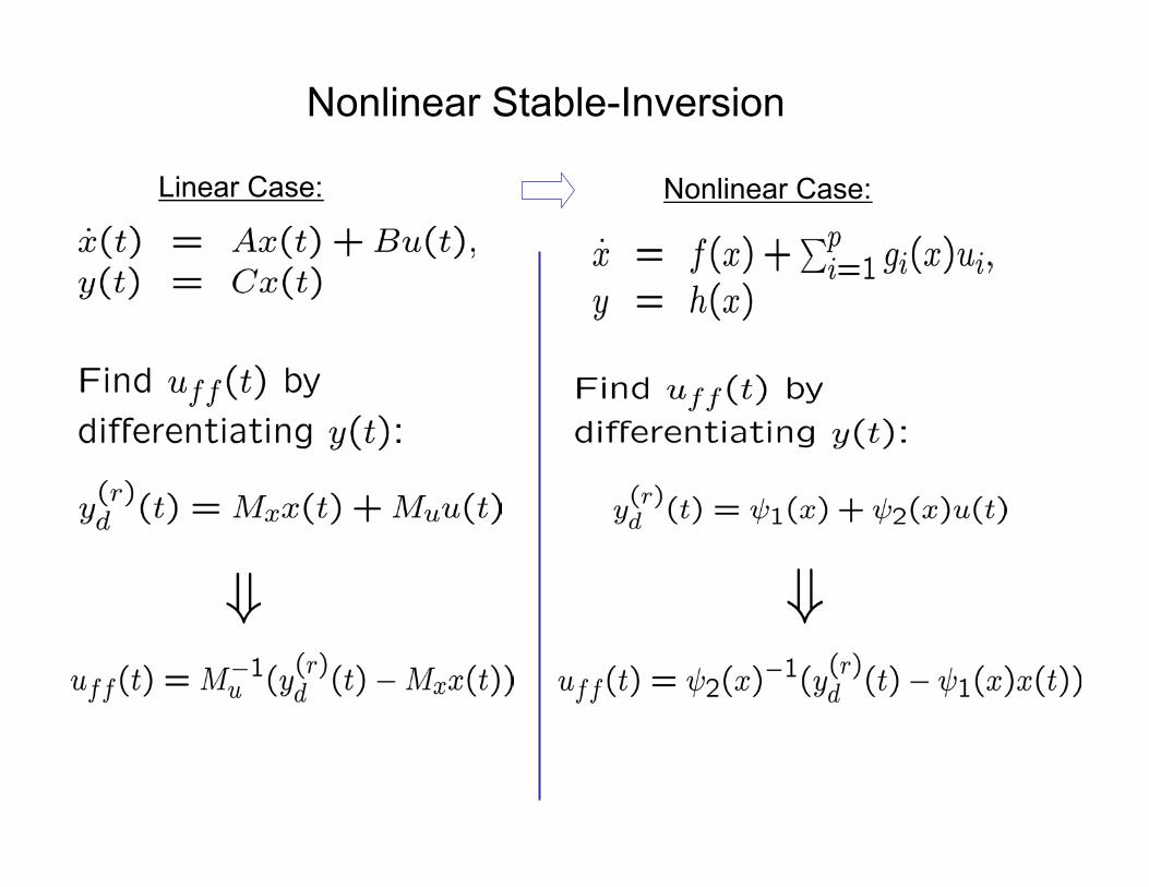
Nonlinear Stable-Inversion
Linear Case: Nonlinear Case:
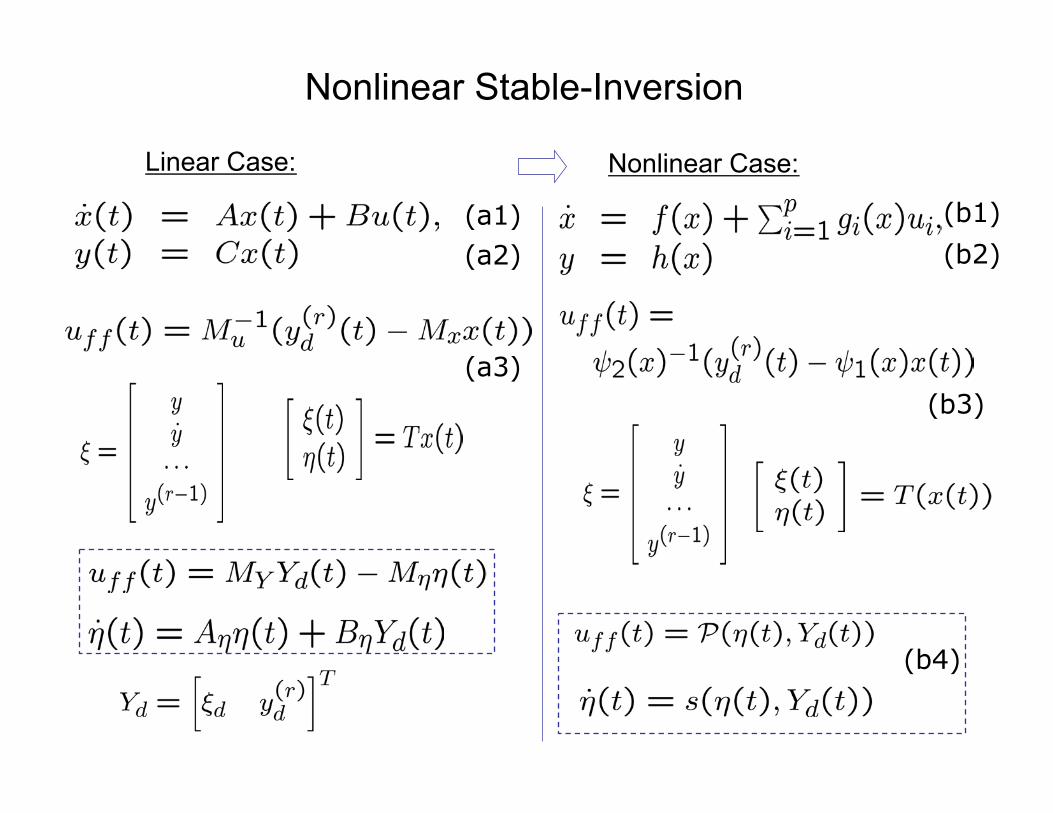
(a1) (a2)
(a3)
(b1) (b2)
(b3)
(b4)
Linear Case: Nonlinear Case:
Nonlinear Stable-Inversion

Solving the nonlinear internal dynamics
(2)
#! Challenge is to prove Convergence: Establish conditions for an argument based on the contraction mapping theorem.
Outline of talk
1.! Brief intro to U. of Washington 2.! Motivation --- nanopositioning 3.! The good and the bad 4.! Approach: Inversion-based feedforward 5.! Connections to ZPET, Robust, Optimal 6.! Experimental Results 7.! The ugly --- unresolved challenges 8.! Conclusions
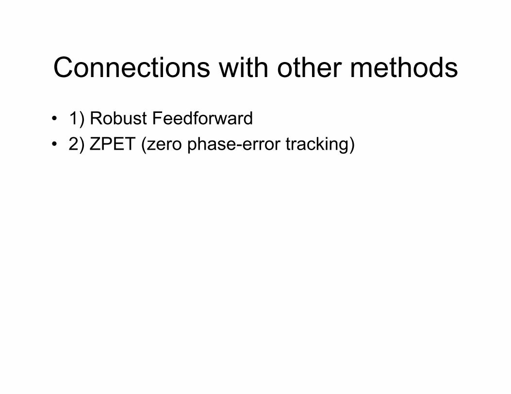
Connections with other methods
•! 1) Robust Feedforward •! 2) ZPET (zero phase-error tracking)
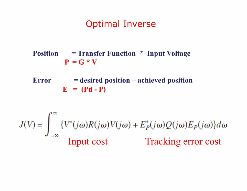
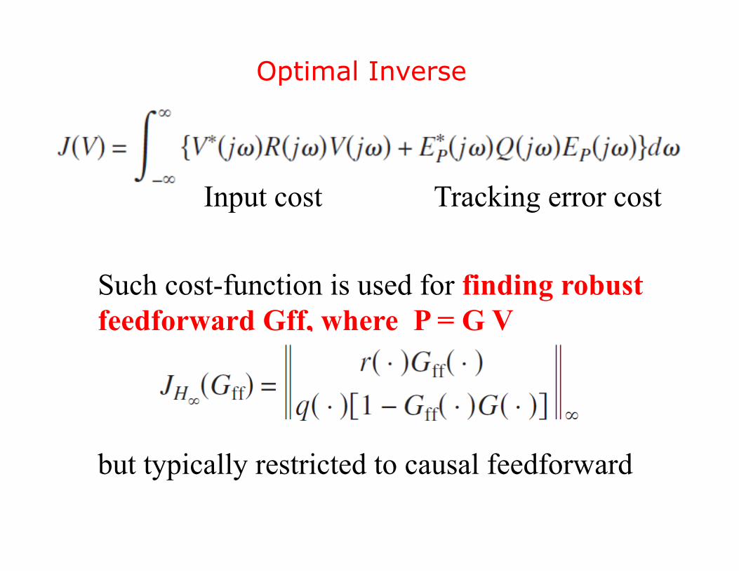
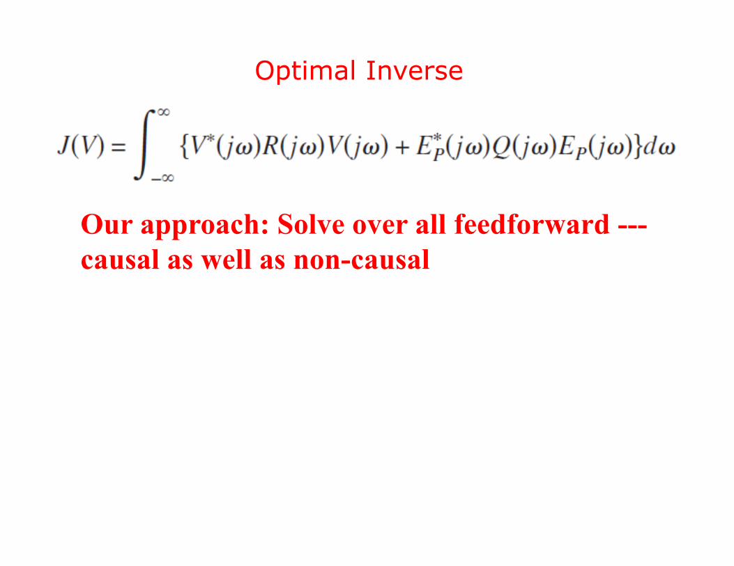
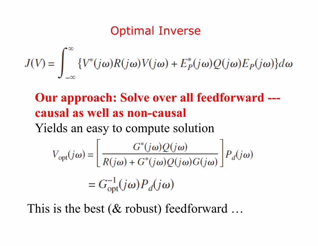
Optimal Inverse
Input cost Tracking error cost
Position = Transfer Function * Input Voltage P = G * V Error = desired position – achieved position E = (Pd - P)
Optimal Inverse
Such cost-function is used for finding robust feedforward Gff, where P = G V but typically restricted to causal feedforward
Input cost Tracking error cost
Optimal Inverse
Our approach: Solve over all feedforward --- causal as well as non-causal
Optimal Inverse
Our approach: Solve over all feedforward --- causal as well as non-causal Yields an easy to compute solution
This is the best (& robust) feedforward …
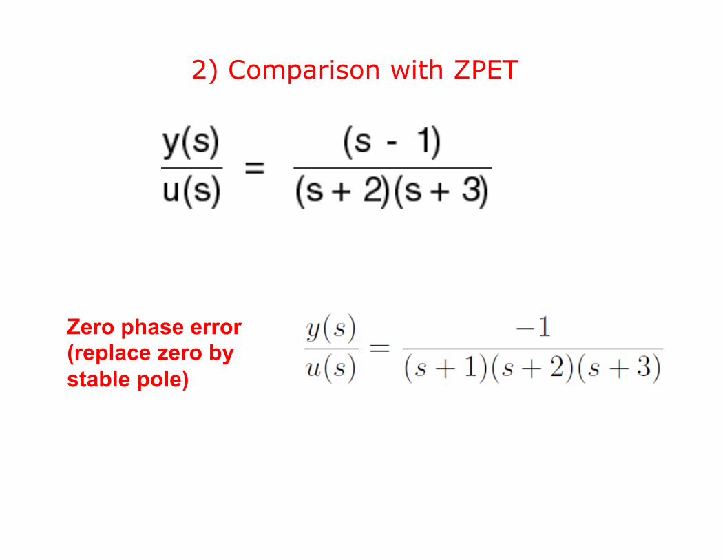
2) Comparison with ZPET
Zero phase error (replace zero by stable pole)
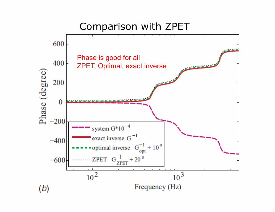
Comparison with ZPET
Phase is good for all ZPET, Optimal, exact inverse
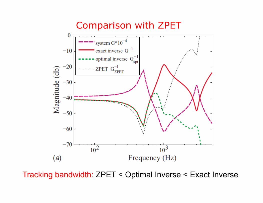
Comparison with ZPET
Tracking bandwidth: ZPET < Optimal Inverse < Exact Inverse
Outline of talk
1.! Brief intro to U. of Washington 2.! Motivation --- nanopositioning 3.! The good and the bad 4.! Approach: Inversion-based feedforward 5.! Connections to ZPET, Robust, Optimal 6.! Experimental Results 7.! The ugly --- unresolved challenges 8.! Conclusions

Nanoscale Positioning in AFM
•! Three problems
•! 1) Creep •! 2) Hysteresis •! 3) Vibrations
Key Issues in Modeling
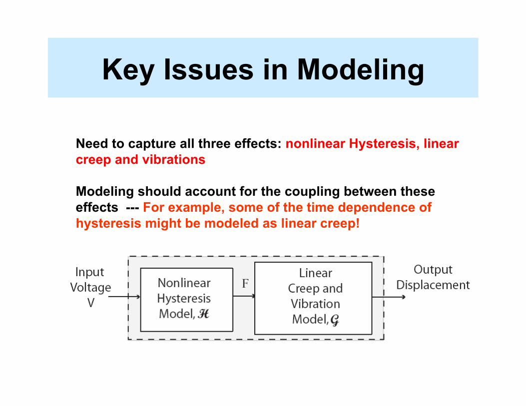
Need to capture all three effects: nonlinear Hysteresis, linear creep and vibrations Modeling should account for the coupling between these effects --- For example, some of the time dependence of hysteresis might be modeled as linear creep!

Use in Piezo Nanopositioners
•! System inverse is used to find input voltages, ua , which compensate for positioner dynamics and achieve the desired output, i.e. y = yd
Input Output Desired Output G0
-1
G
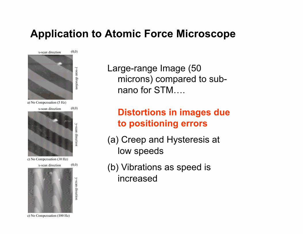
Application to Atomic Force Microscope
Large-range Image (50 microns) compared to sub-nano for STM!. Distortions in images due to positioning errors
(a)! Creep and Hysteresis at low speeds
(b)! Vibrations as speed is increased
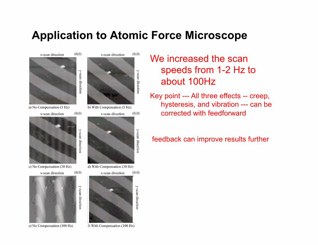
We increased the scan speeds from 1-2 Hz to about 100Hz
Key point --- All three effects -- creep, hysteresis, and vibration --- can be corrected with feedforward
feedback can improve results further
Application to Atomic Force Microscope
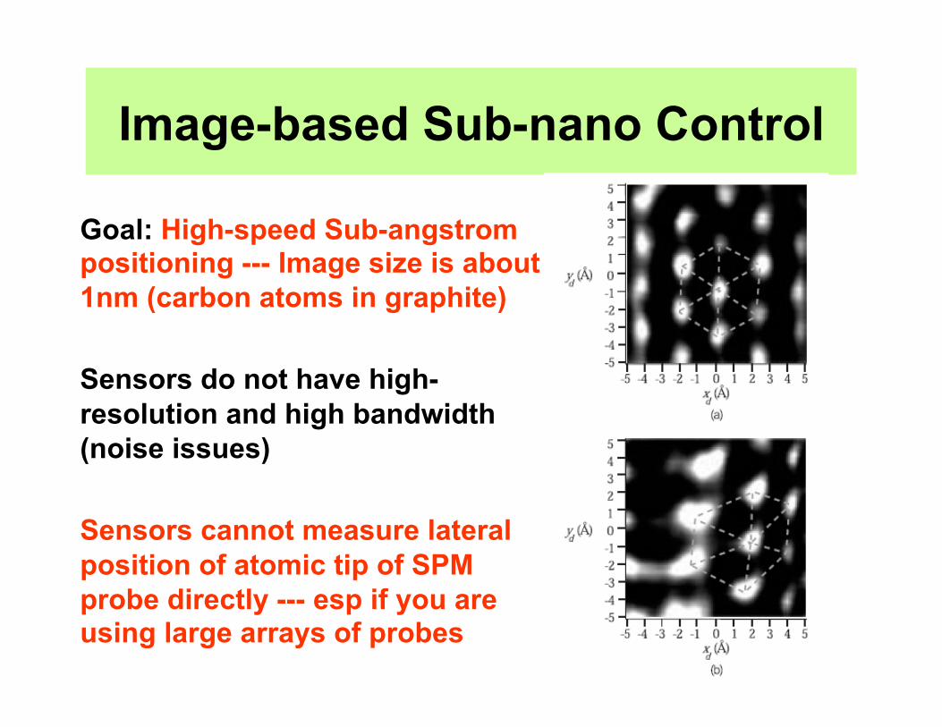
Image-based Sub-nano Control
Goal: High-speed Sub-angstrom positioning --- Image size is about 1nm (carbon atoms in graphite) Sensors do not have high-resolution and high bandwidth (noise issues) Sensors cannot measure lateral position of atomic tip of SPM probe directly --- esp if you are using large arrays of probes
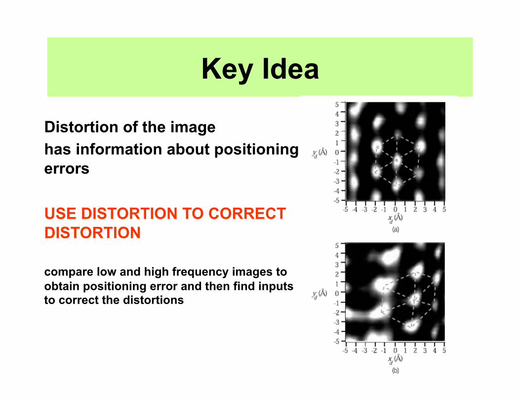
Key Idea
Distortion of the image has information about positioning errors USE DISTORTION TO CORRECT DISTORTION compare low and high frequency images to obtain positioning error and then find inputs to correct the distortions
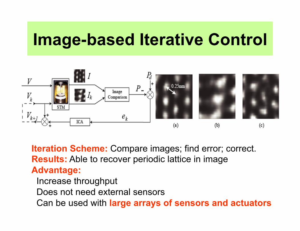
Image-based Iterative Control
Iteration Scheme: Compare images; find error; correct. Results: Able to recover periodic lattice in image Advantage: Increase throughput Does not need external sensors Can be used with large arrays of sensors and actuators

Current Efforts
•! Imaging Soft Samples: in particular micro-vascular endothelial cells
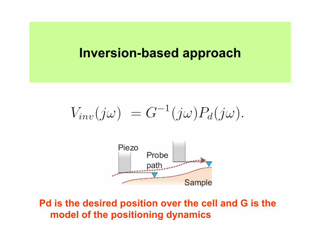
Inversion-based approach
Pd is the desired position over the cell and G is the model of the positioning dynamics
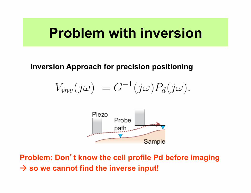
Problem with inversion
Inversion Approach for precision positioning
Problem: Don t know the cell profile Pd before imaging "" so we cannot find the inverse input!
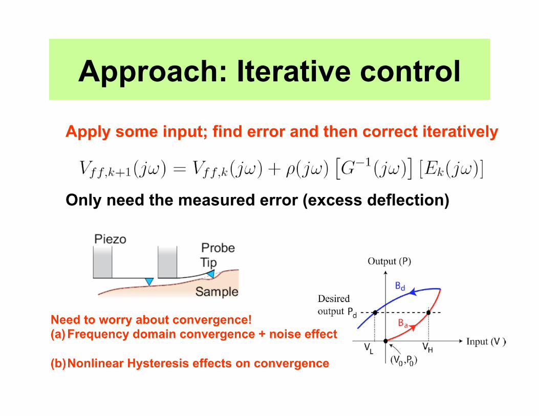
Approach: Iterative control
Apply some input; find error and then correct iteratively
Only need the measured error (excess deflection)
Need to worry about convergence! (a)!Frequency domain convergence + noise effect
(b)!Nonlinear Hysteresis effects on convergence
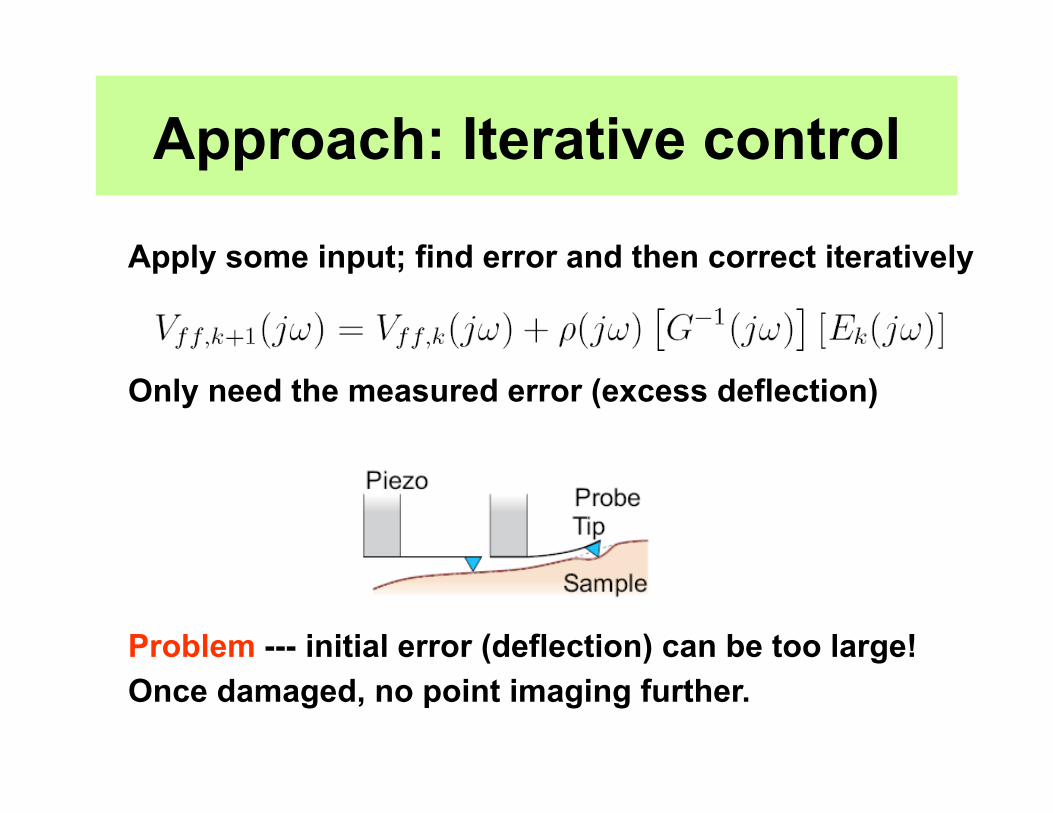
Approach: Iterative control
Apply some input; find error and then correct iteratively
Only need the measured error (excess deflection)
Problem --- initial error (deflection) can be too large! Once damaged, no point imaging further.

Zoom-out/Zoom-in Approach Still use iterative control
Increase scan area slowly "" initial height changes are small "" initial deflection (forces) are small
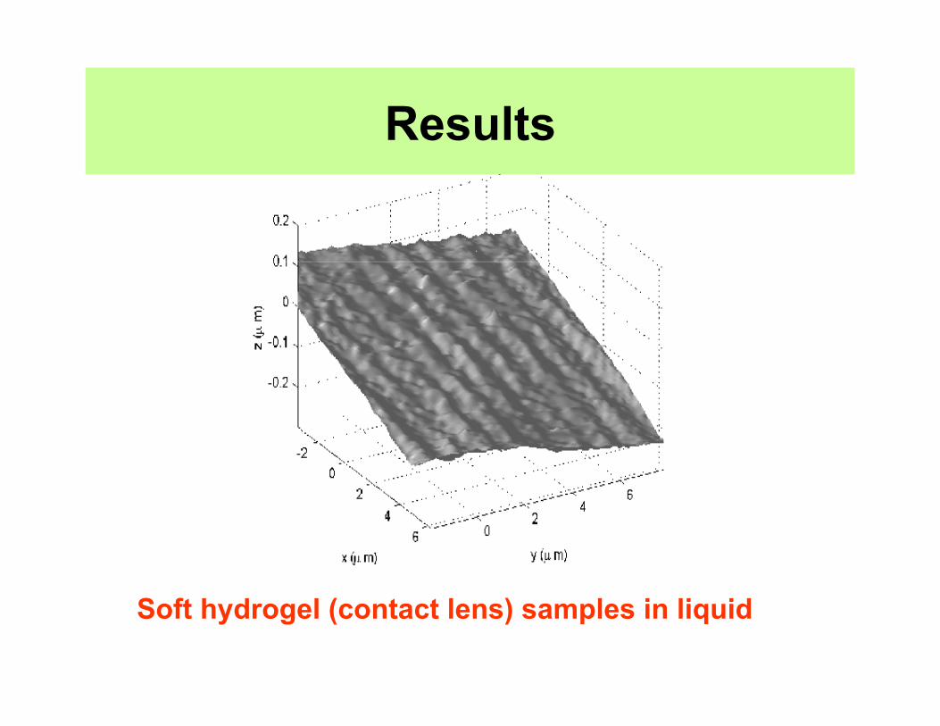
Results
Soft hydrogel (contact lens) samples in liquid
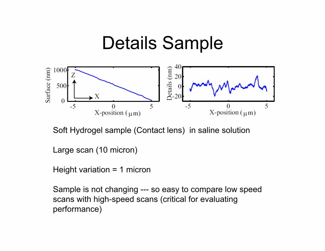
Details Sample
Soft Hydrogel sample (Contact lens) in saline solution Large scan (10 micron) Height variation = 1 micron Sample is not changing --- so easy to compare low speed scans with high-speed scans (critical for evaluating performance)

Able to image at 30 Hz
30 Hz
Forces are less than 500 pN
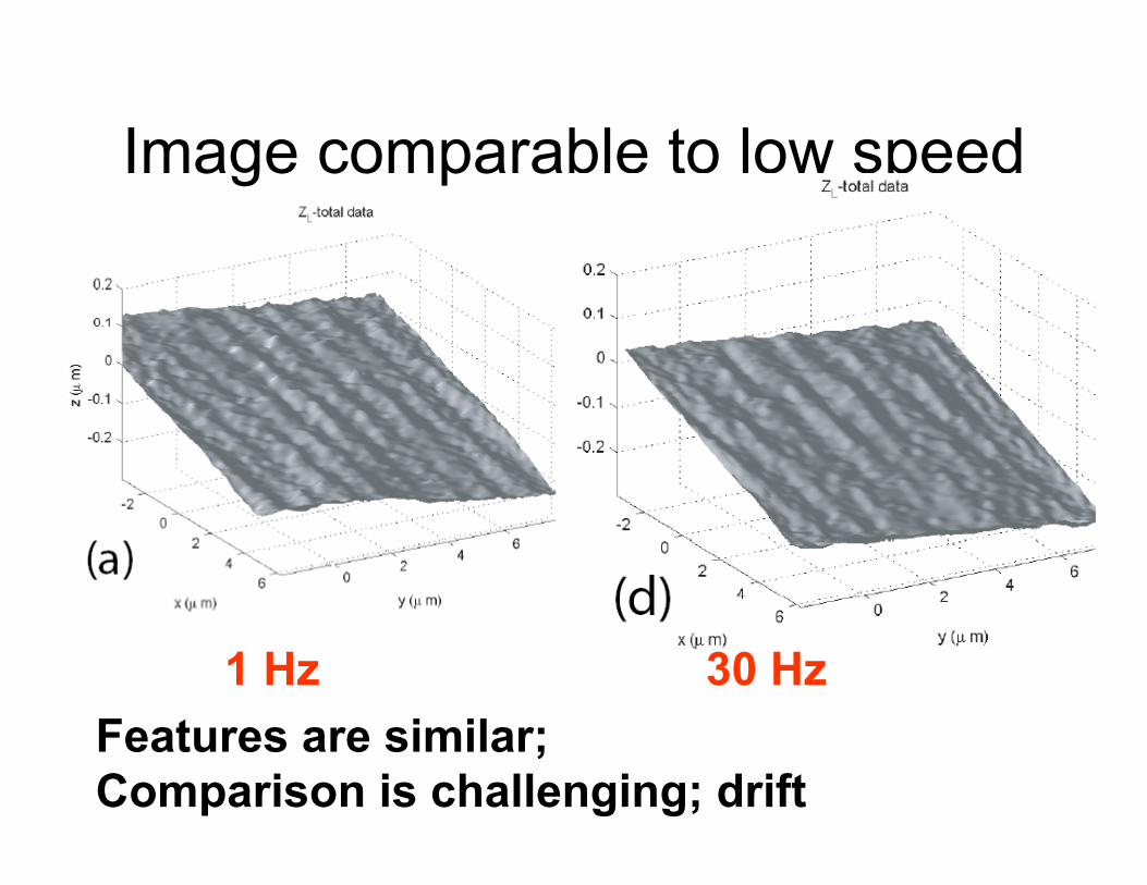
Image comparable to low speed
1 Hz 30 Hz
Features are similar; Comparison is challenging; drift
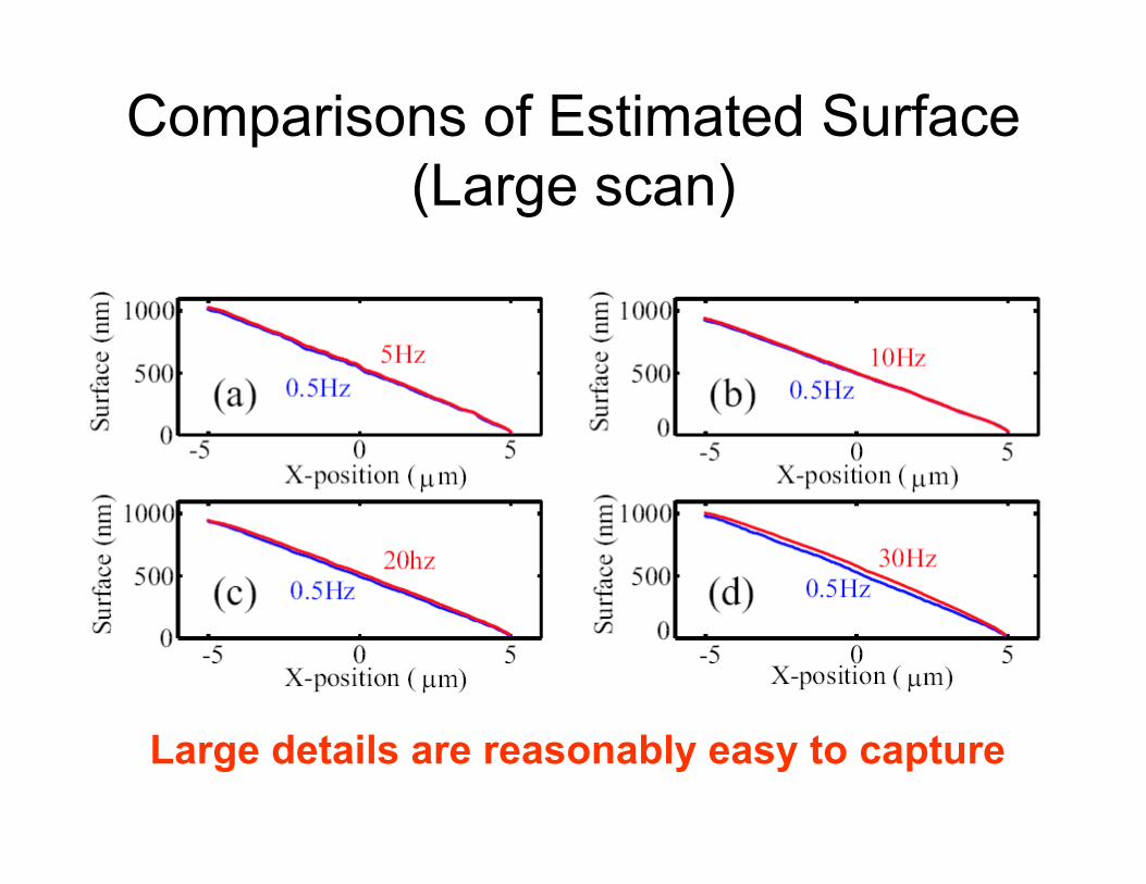
Comparisons of Estimated Surface (Large scan)
Large details are reasonably easy to capture
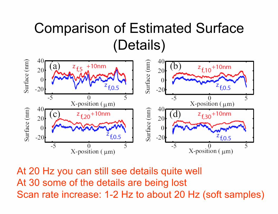
Comparison of Estimated Surface (Details)
At 20 Hz you can still see details quite well At 30 some of the details are being lost Scan rate increase: 1-2 Hz to about 20 Hz (soft samples)
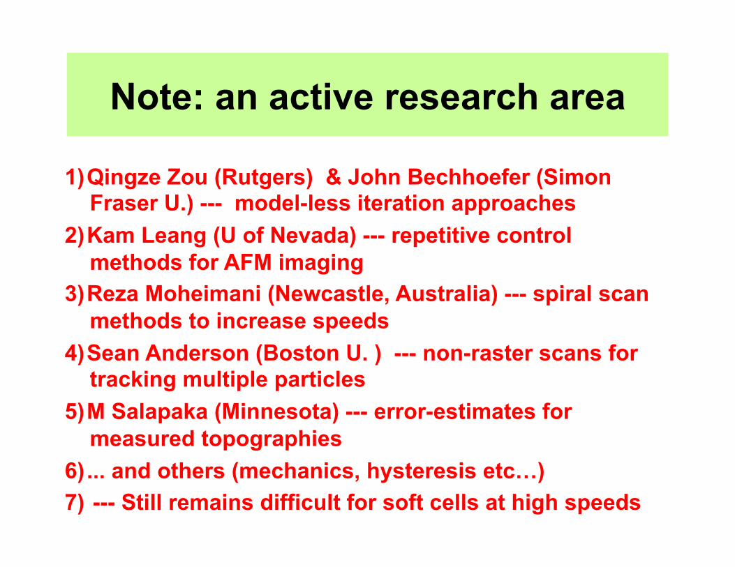
Note: an active research area
1)!Qingze Zou (Rutgers) & John Bechhoefer (Simon Fraser U.) --- model-less iteration approaches
2)!Kam Leang (U of Nevada) --- repetitive control methods for AFM imaging
3)!Reza Moheimani (Newcastle, Australia) --- spiral scan methods to increase speeds
4)!Sean Anderson (Boston U. ) --- non-raster scans for tracking multiple particles
5)!M Salapaka (Minnesota) --- error-estimates for measured topographies
6)! ... and others (mechanics, hysteresis etc!) 7)! --- Still remains difficult for soft cells at high speeds
Outline of talk
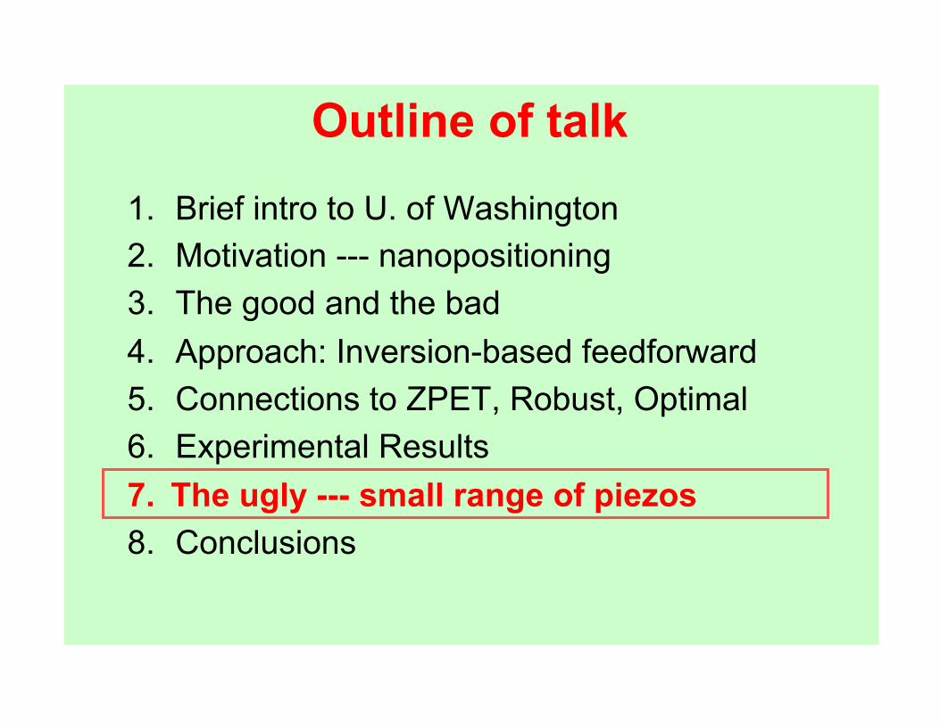
1.! Brief intro to U. of Washington 2.! Motivation --- nanopositioning 3.! The good and the bad 4.! Approach: Inversion-based feedforward 5.! Connections to ZPET, Robust, Optimal 6.! Experimental Results 7.! The ugly --- small range of piezos 8.! Conclusions

The good, the bad, and the ugly
Piezos have small range

Piezos have small range --- larger piezos have smaller bandwidth
Ref: Review article in ASME J Dy. Systems, Meas. and Control, 2009
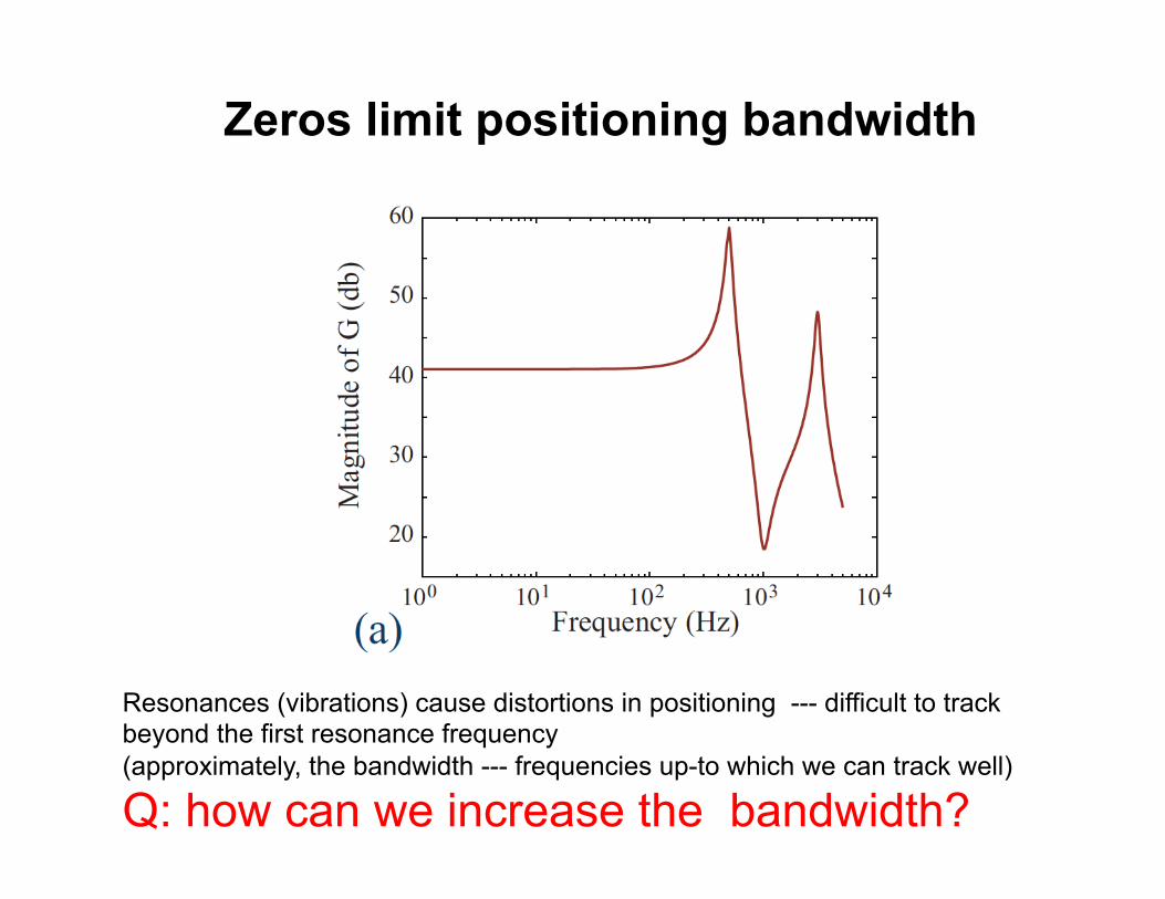
Zeros limit positioning bandwidth
Resonances (vibrations) cause distortions in positioning --- difficult to track beyond the first resonance frequency (approximately, the bandwidth --- frequencies up-to which we can track well)
Q: how can we increase the bandwidth?
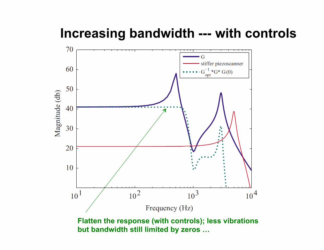
Increasing bandwidth --- with controls
Flatten the response (with controls); less vibrations but bandwidth still limited by zeros !
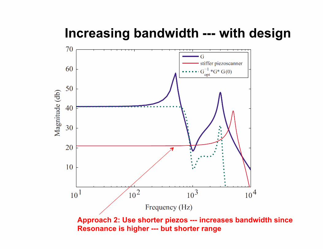
Increasing bandwidth --- with design
Approach 2: Use shorter piezos --- increases bandwidth since Resonance is higher --- but shorter range

Why? Resonance Frequency is inversely proportional to Size (L2)
•! First resonance freq (possible
bandwidth) increases as dimensions get smaller
•! Piezo-tube L= length, D = Diameter, h= thickness %=Density, E=Youngs Modulus
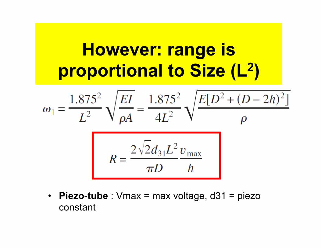
However: range is proportional to Size (L2)
•! Piezo-tube : Vmax = max voltage, d31 = piezo
constant
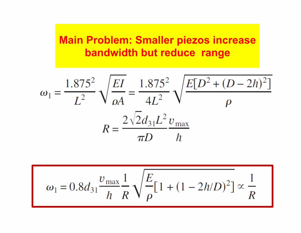
Main Problem: Smaller piezos increase bandwidth but reduce range
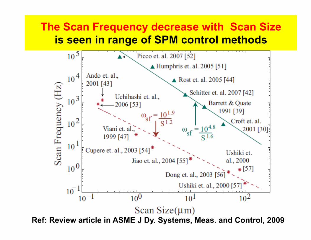
The Scan Frequency decrease with Scan Size is seen in range of SPM control methods
Ref: Review article in ASME J Dy. Systems, Meas. and Control, 2009
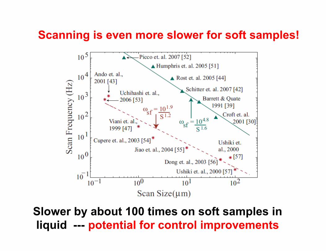
Scanning is even more slower for soft samples!
Slower by about 100 times on soft samples in liquid --- potential for control improvements
An unresolved issue in nanopositioning
Want high precision (piezo type positioner)
but
We also want high bandwidth & large range
Main Concept --- stepping
Piezos are small "" small step (high bandwidth)
multiple steps "" large overall range
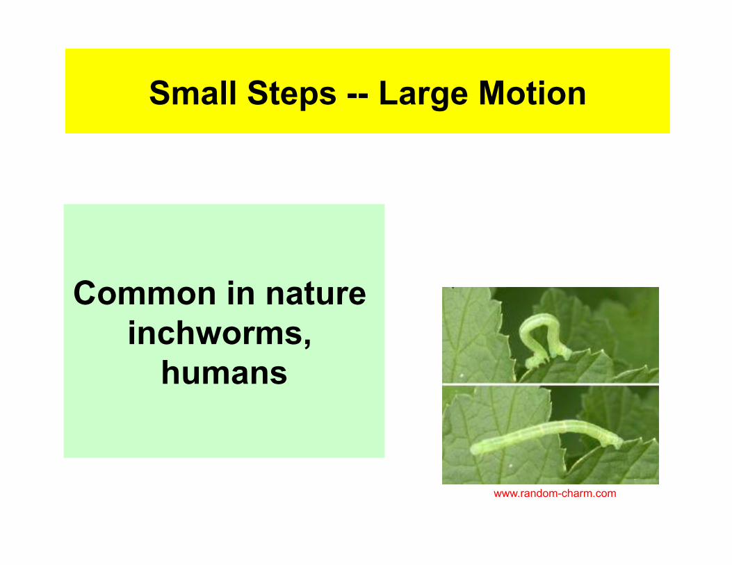
Small Steps -- Large Motion
www.random-charm.com
Common in nature inchworms,
humans
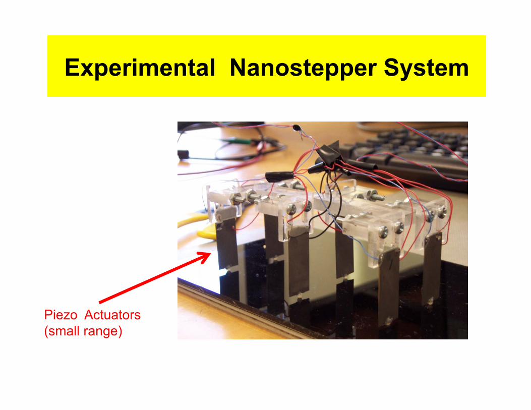
Experimental Nanostepper System
Piezo Actuators (small range)

Videos
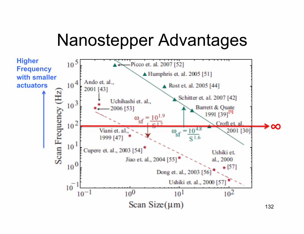
Nanostepper Advantages
[1]
"
Higher Frequency with smaller actuators
132
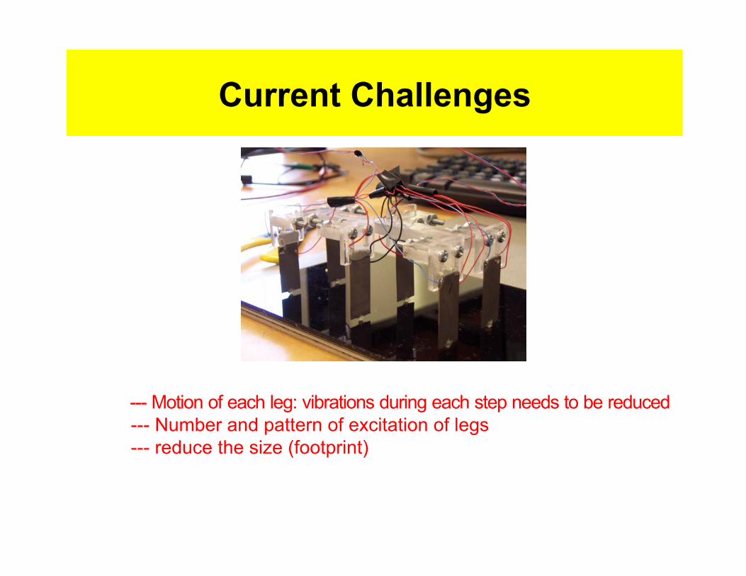
Current Challenges
--- Motion of each leg: vibrations during each step needs to be reduced --- Number and pattern of excitation of legs --- reduce the size (footprint)
Outline of talk
1.! Brief intro to U. of Washington 2.! Motivation --- nanopositioning 3.! The good and the bad 4.! Approach: Inversion-based feedforward 5.! Connections to ZPET, Robust, Optimal 6.! Experimental Results 7.! The ugly --- unresolved challenges 8.! Conclusions

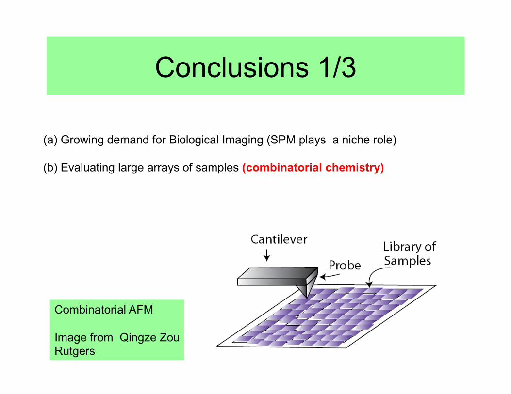
(a)!Growing demand for Biological Imaging (SPM plays a niche role)
Conclusions 1/3
(a)!Growing demand for Biological Imaging (SPM plays a niche role)
(b)!Evaluating large arrays of samples (combinatorial chemistry)
Conclusions 1/3
Combinatorial AFM Image from Qingze Zou Rutgers

(a)!Growing demand for Biological Imaging (SPM plays a niche role)
(b)!Evaluating large arrays of samples
Conclusions 1/3
•! Increase Precision: large errors lead to large forces (imaging soft samples), wrong features (distortions in nanofabrication) •! Increase Range: Nanofeatures imaged/fabricated over tens of micron •! Increase Bandwidth: Increase throughput of imaging/fabrication " parallelism
Main Themes
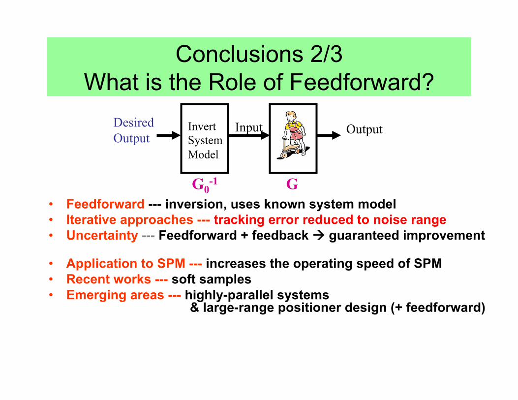
Conclusions 2/3 What is the Role of Feedforward?
•! Feedforward --- inversion, uses known system model •! Iterative approaches --- tracking error reduced to noise range •! Uncertainty --- Feedforward + feedback "" guaranteed improvement
•! Application to SPM --- increases the operating speed of SPM •! Recent works --- soft samples •! Emerging areas --- highly-parallel systems
& large-range positioner design (+ feedforward)
Input Output Invert System Model
Desired Output
G0-1 G

Conclusions 3/3 Positioning is an intellectually rich area
Broad applications 1)! Nanotechnologies (SPM) 2)! Disk Drive Industries (Dual-stage) 3)! Aircraft Control (VTOL hover control) 4)! Robotics
Neat Theory Problems 1)! Is it possible to achieve a given
position trajectory?
2)! If so, how do we find the input to achieve it?
3)! If not, how do you re-design the trajectory (optimally)?
Some advantages of working in positioning 1)! Can choose from a large set of areas for research (broad applications) 2)! Fundamental theoretical issues 3)! Nice interaction between theory and application
Thank You