0

FEDERAL DEMOCRATIC REPUBLIC OF ETHIOPIA

HOUSE OF FEDERATION

The Federal General-Purpose Grant Distribution

Formula 2017/18 - 2019/20

Addis Ababa, Ethiopia

June, 2017

1

Contents CHAPTER ONE: INTRODUCTION ......................................................................................... 2

1.1. Background and Rationale ............................................................................................................ 4

1.2. Objective and Scope of the study .................................................................................................. 6

1.2.1. Objectives of the Study ................................................................................................... 6

1.2.2. Scope of the Study .......................................................................................................... 7

1.3. Organization .................................................................................................................................. 7

CHAPTER TWO: THE LITERATURE AND CONCEPTUAL FRAMEWORK ............... 8

2.1. Approaches to fiscal gap estimation: An overview ............................................................................ 8

2.2 Conceptual framework ...................................................................................................................... 11

CHAPTER THREE: POTENTIAL REVENUE RAINSING CAPACITY OF REGIONAL STATES ................................................................................................................ 14

3.1. Introduction ...................................................................................................................................... 14

3.2. What has been improved .................................................................................................................. 14

3.3. Representative tax system (RTS) ..................................................................................................... 14

3.4. The revenue sources ......................................................................................................................... 15

3.5. Identification of the Tax Base and Computation of the Weighted Average Tax Rate ..................... 16

3.5.1. Agricultural income tax ...................................................................................................... 16

3.5.2. Agricultural land use fee ..................................................................................................... 19

3.5.3. Payroll tax ........................................................................................................................... 22

3.5.4. Turnover tax (TOT) ............................................................................................................ 25

3.5.5. Business income tax (profit tax) ......................................................................................... 26

3.6. Regional revenue raising potential ................................................................................................... 34

3.7. Total regional revenue potential ...................................................................................................... 36

Appendices .............................................................................................................................................. 37

CHAPTER FOUR: ESTIMATION of EXPENDITURE NEEDS of REGIONS .................. 41

4.1. Estimation Approach ....................................................................................................................... 41

4.2. Actual Expenditures of the Regional States and their Compositions............................................... 47

4.3. The measurement units and adjustment factors for the major expenditure categories .................... 49

2

4.3.1. General Service and administration (Organ of the state, Justice and security, and general service) .......................................................................................................................................... 49

4.3.2. Primary and secondary education (including TVET) ......................................................... 57

4.3.3. Public Health ....................................................................................................................... 63

4.3.4: Agriculture and Rural development .................................................................................... 66

4.3.6: Rural Road Construction and Maintenance ........................................................................ 69

4.3.7. Urban Development ............................................................................................................ 73

4.3.8. Micro and Small-Scale Enterprise (MSE) development ..................................................... 74

4.3.9. Spatial Price Index .............................................................................................................. 78

CHAPTER FIVE: TOTAL AND RELATIVE FISCAL GAPS OF REGIONAL STATES ....................................................................................................................................... 80

CHAPTER SIX: CONCLUDING REMARKS AND RECOMMENDATIONS .................. 80

6.1. Conclusions ...................................................................................................................................... 81

CHAPTER SEVEN: DECISION OF THE HOUSE OF FEDERATION ............................. 83

2

Message from the Speaker of the House of Federation

The Constitution of the Federal Democratic Republic of Ethiopia in article 62(4) stipulates that the grant from the federal government to regional states is distributed according to the grant distribution formula endorsed by the House of Federation (HoF). Regional states currently cover the largest proportion of the expenditures with the grant they receive from the federal government. Consequently, it is not overstatement to conclude that the grant from the federal government is the main revenue source for regional states. As a result, the distribution of this grant among regional states is a task that requires the highest possible efforts and serious attentions. To make the distribution of the grant just and effective it is crucial to draw lessons from other federal countries, strengthen the capacity of the staff that provide the House with professional support, and improve the awareness and understanding of the members of the HoF. Though efforts have been made in this regard, the House believes that a lot remains to be improved and there are many tasks that require more efforts.

This grant formula, which is endorsed by the House to serve for the three years period of 2010-2012 E.C., required the cooperation and efforts of many for its preparation. One key difference of this grant formula is that though its preparation, like the formulas prepared in the past, required the support of consultants, for the first time the body that played the consulting role is an institution, not individuals. The consulting team from Economics Department of Addis Ababa University together with the professionals from the HoF made robust effort in identifying the limitations of the previous formula and recommending and including the improvements deemed necessary into the new formula.

There had been continuous engagement and discussions with stakeholders at different stages of the preparation of this grant formula. Furthermore, as much as the circumstances in the country with respect to availability and quality of data allowed, efforts were made to ensure that the grant formula is based on reliable and acceptable data. For few expenditure items for which data were not available at federal institutions, the standing committee for budget grants and revenue sharing was requested to make decisions and provide directions. Thus, the questions related to such items were addressed and they were included in to the grant formula based on the directions put in place by the standing committee. Even though all members of the standing committee and all regional states agreed on the framework of the grant formula and the preparation process, according to the new formula the share of few regional states declined in absolute terms compared to what they were receiving as per the old formula. Since it was believed that some of these regional states cannot bear the burden of these change, based on political negotiations, adjustments were made by deducting from those regions whose shares increased in relative terms as per the new formula. These types of initiatives and cooperation among regional states to support each other and share each other’s burdens need to be encouraged.

As per the lessons drawn from the preparation process of the current grant formula and also based on the recommendations of the consultants, enough time should be given for the

3

preparation of the next grant formula. Accordingly, facilitation works will be done to start the preparation of the grant formula that will be used starting in 2013 E.C. as early as possible. It is believed that such a process will lead to further improvements of the current grant formula.

Finally, on behalf of the House and myself, I would like to take this opportunity to extend my thanks to those who supported the efforts of the House by availing data and providing inputs during discussions on the grant formula framework. Furthermore, I would like to extend my thanks to the consultants and the professionals of the House for their diligence to complete the preparation of the grant formula in relatively short period of time. My thanks also go to different institutions which, in one way or another, supported the preparation of the grant formula. The participation and support of stakeholders and other collaborating institutions are crucial for all our works. Thus, I would like to indicate the readiness of the House to work with all stakeholders and other collaborating institutions and call upon all concerned bodies to continue their support taking into account the national importance of the works of the House.

Yalew Abate

Speaker of the House of Federation

4

CHAPTER ONE: INTRODUCTION 1.1. Background and Rationale

The pre-1991/92 Ethiopia was ruled by governments that can be classified as unitary type of

governments. But after the Ethiopian Peoples Revolutionary Democratic Front (EPRDF) came to

power in 1991/92, the system of administration has been changed into a federal system. Under a

federal system, the decision-making powers are shared across multi-leveled governments.Improving

the resource mobilization and allocation efficiencies of the public sector,addressing diversity issues

(like self-governance, ethnicity, culture, history), creating an enabling business environment for the

private sector, and fast and sustainable national economic growthare some of the justifications for the

adoption of decentralized system of administration.

In Ethiopia, the federal system started during the transition period (1991-1995) and this system was

ratified when the country adopted the constitution in 1995. According to the Constitution, the

Ethiopian federation constitutes the federal government, nine regional states and one administrative

city.1There are no legal boundaries among regions. The responsibilities and functions assigned to the

federal andregional governments are also stated in the 1995 constitution.

The Constitution stipulates the powers and functions of the Federal Government and that of the States

in Article 51 and 52, respectively. One of the outcomes of these assignments of functions to the

Federal and State governments is Fiscal federalism where the constitution assigned different

responsibilities and functions to the federal and regional governments. The responsibilities and

functions regarding the financial expenditures are stated in Article 94 of the constitution. For instance,

Article 94 (1) states that “the federal government and the states shall respectively bear all financial

expenditures necessary to carry out all responsibilities and functions assigned to them by the law.”

Article 94 (2) adds that “The federal government may grant to states emergency, rehabilitation, and

development assistance and loans, due care being taken such that the assistance and loan do not hinder

the proportionate development of other states.” The responsibilities and functions of tax collection for

the federal government and regional governments are, respectively, specified in Articles 96 and 97

while concurrent tax collections are statedin article 98.

As is the case in most federal governments, there is significant vertical fiscal gap in Ethiopia due to

the imbalance between the expenditure needs (that arise from functions assigned) and revenue

generating capacity of regional states. This fiscal gap has been covered relatively by the general-

purpose grant provided by the federal government to the states. Since there are large heterogeneities

1 The nine regional states are Tigray, Afar, Amhara, Oromia, Somali, Benishangul-Gumuz, SNNP, Harari and Gambella while the Administrative City is the capital Addis Ababa.

5

across the regions in terms of population size, levels of development, poverty, tax collections, and

expenditures, the absoluteand relative size of the subsidy transferred to regions vary considerably to

reflect the heterogeneities. The grant distributions from the federal government to the regional

governments are based on five provisions which are stated in the following articles of the constitution.

These are:

i) Article 41(3): Every Ethiopian national has the right to equal access to publicly funded social

services,

ii) Article 89(2): Government has the duty to ensure that all Ethiopians get equal opportunity to

improve their economic conditions and to promote equitable distribution of wealth among

them,

iii) Article 89(4): Nations and Nationalities and Peoples least advantaged in economic and social

development shall receive special assistance,

iv) Article 94(1): The Federal Government and the States shall respectively bear all the financial

expenditure necessary to carry out all responsibilities and functions assigned to them by law.

Unless otherwise agreed upon, the financial expenditures required for carrying out of any

delegated function by the state shall be borne by the delegating party; and

v) Article 94(2): The Federal Government may grant the States emergency, rehabilitation, and

development assistance and loans, due care being taken that such assistance and loans do not

hinder the proportionate development of States. The Federal Government shall have the

power to audit and inspect the proper utilization of subsidies it grants to the States.

Intergovernmental fiscal transfersfinance about 60 percent of sub-national expenditures in developing

countries and transition economies and about a third of such expenditures in OECD countries (29

percent in the Nordic countries, 46 percent in non-Nordic Europe). Beyond the expenditures they

finance, these transfers create incentives and accountability mechanisms that affect the fiscal

management, efficiency, and equity of public service provision and government accountability to

citizens. And, countries use different institutional set up andsystem to manage and allocate

intergovernmental fiscal transfer depending on their specific set of conditions.

In the case of Ethiopia, the responsibility of deciding the proportion of the grant allocation to the

regions is constitutionally vested on the House of Federation (HoF). In this regard, Article 62 (7)

states that “the HoF shall determine the division of revenues derived from joint Federal and State tax

sources and the subsidies that the Federal Government may provide to the States.” The HoF has been

exercising the powers of deciding the proportion of subsidies allocated to each region and the other

responsibilities and functions since 1994/95.HoF has been adopting a subsidy allocation formula in

order to capture the relative fiscal gaps of the States as accurately as possible. Moreover, HoF revises

the subsidy allocation formula periodically so as to adjust the federal subsidy allocation to the changes

6

in the socio-economic conditions in each State and also improve weaknesses of the formulae from

time to time. A number of grant formulae were developed and used since the country adopted fiscal

federalism. The current federal grant distribution formula has been used since 2012; that is for the last

5 years. HoF has intended to use a revised formula starting from 2017.The revision is necessary to

adjust the proportion of the subsidy allocated to each region to the changes in population size, levels

of development, revenue collection capacities, employment, and poverty among others across the

regions. In this regard, HoF distributed a Terms of Reference (TOR) which describes the main

principles of the revised formula along with the types of data and methodologies for revising the

subsidy distribution formula, and the expected results of the study.

The TOR emphasizes four principles. The first principle stipulates that the revised formula should be

simple. In other words, the formula should replace the fuzzy and difficult methods of calculating the

regional governments’ revenue raising capacities and expenditure needs with simple and clear

computation methods and approaches. Secondly, the ToR requires that the revision should use all the

indicators which were employed for calculating the formula under current use. Thirdly, correcting

unreliable and questionable values of permanent expenditures used in the formula currently in use

with better quality data and valid methods in the revised formula. Finally, the TOR specifies the need

for replacing unrealistic estimates of expenditure and revenue with improved estimation approaches.

1.2. Objective and Scope of the study

1.2.1. Objectives of the Study

The main objective of this study is revising the current Federal subsidy allocation formula to ensure

more equitable and efficient resource allocations. The specific objectives of the study are:

i. Identifying and developing efficient and easy techniques of assessing and estimating the

regional expenditure needs and revenue generating capacity,

ii. Collect data of expenditure and revenue of the past three years by regional States so as to

update the data previously used in developing the current transfer allocation formula,

iii. Update the existing regional level estimates of the spatial price index,

iv. Update the regular and potential expenditure needs and revenue raising capacity estimates

based on regions’ expenditure responsibilities and revenue raising authority given by the

constitution,

v. Replacing computations made with earlier assumptions and method on revenue capacities

with improved methods in the current allocation formula.

7

1.2.2. Scope of the Study

While the development of the new Federal General-Purpose Grant Allocation Formula is made within

the framework of the existing one, the scope of work will include additional efforts specified in the

objectives above.

1.3. Organization This document is organized in seven chapters. Following this introductory chapter, chapter two deals

with the developments of the different types of intergovernmental fiscal transfers and the different

approaches used to estimate the transfers. Chapter three presents the methodology employed to

estimate the fiscal capacity of regional states and the estimated potential revenue of the regional

states. In a similar fashion, chapter four discusses the details of the representative expenditure

approach used and the steps followed to estimate the expenditure needs of the regional states and the

estimated expenditure needs for each region for each of the main expenditure categories selected.

Chapter five combines the total estimated expenditure needs of regions corrected for spatial price

differences with the total estimated potential revenue of regions and generates total and relative fiscal

gaps of regional states. Chapter six, based on the lessons learned in the process of developing this

Federal General-Purpose Grant Formula, presents concluding remarks and recommendations that are

believed to be crucial for the development of future grant formulas. Chapter seven presents the final

formula that is endorsed by the House of Federation of FDRE.

8

CHAPTER TWO: THE LITERATUREANDCONCEPTUAL FRAMEWORK

2.1. Approaches to fiscal gap estimation: An overview

The literature provides different approaches to estimate fiscal gap. Funds can be transferred from the

federal government to sub-national governments through political negotiations, or on an ad hoc basis,

or using a formula-based equalization transfer system. Each approach has its own advantages and

disadvantages in terms of data requirements and in ensuring that the fundamental principles and

provisions of the Constitution are strictly adhered to.

In the political negotiation approach, the federal government bargains and negotiates with regional

governments in allocating funds. This approach is less transparent and gives discretionary power to

the federal government in determining the expenditure needs of each region.

In the ad-hoc approach, the federal government determines the amount of fund to be transferred to

each region using simple measures of expenditure needs. However, this approach lacks scientific

measurements of fiscal capacities and fiscal needs of each sub-national government. This can easily

lead to an unjustified distribution of funds and encourage the regions' bargaining activities. It may

also undermine local autonomy, flexibility, fiscal efficiency, and fiscal equity objectives. In general,

ad-hoc grants are unlikely to result in behavioral responses that are consistent with the federal

government's objectives and such grants may create budgetary difficulties for the federal government.

The formula-based equalization transfer system, if properly designed, is preferred over the political

negotiation and ad-hoc approaches mainly because it meets prevailing international norms and

practices in intergovernmental fiscal transfers or federal allocation of funds. It also increases the

likelihood of satisfying constitutional and legal principles such as: vertical and horizontal equity,

efficiency, revenue adequacy, predictability, transparency, accountability, and autonomy. A budget -

subsidy-allocation formula will satisfy vertical equity if it ensures that the revenue of a region is

consistent with its expenditure responsibilities and needs, while, horizontal equity is achieved when

two regions with the same expenditure needs but different tax bases are able to provide a comparable

level of service at comparable tax rates.

A budget allocation formula is said to be efficient, if it is neutral with respect to sub-national

government choices of resource allocation to different sectors or different types of activity. It should

also help regions to have adequate revenues to discharge designated responsibilities and provide

sufficient revenue for socio-economic development and provision of public services.

According to the literature on fiscal decentralization (Barati and Szalai, 2000; Boadway, 2004; Rosen

2005; Shah 2005a and Shah 2005b), there are four broad types of formula-based equalization transfer

9

systems: Revenue Raising Capacity Equalization (RRCE) Formula; Expenditure Need Equalization

(ENE) Formula; Equal Per Capita Equalization (EPCE) Formula; and Expenditure Need and Revenue

Raising Capacity Equalization (ENRRCE) Formula.

(a) Revenue Raising Capacity Equalization (RRCE) Formula:

This formula is based only on the estimates of the ability of each region to raise revenue from its own

sources. This capacity is estimated either using macroeconomic indicators or using the representative

tax system. Among macroeconomic indicators, state GDP, state factor income, state personal income

and personal disposable income are used to measure a region’s ability to raise revenue. The state GDP

represents the total value of goods and services produced within a state. However, it is not a perfect

indicator of the ability of a regional government to raise taxes because significant portion of the

income may accrue to non-resident owners of factors of production. State factor income, on the other

hand, includes capital and labour income earned in the state. Nevertheless, it makes no distinction

between income earned and income retained by residents of that region. State personal income is the

sum of all income received by residents of a given state (region) while, personal disposable income is

personal income minus direct and indirect taxes plus transfers. Although both personal income and

personal disposable income are reasonable measures of a region’s ability to raise revenue, they are

only partial measures of the ability to impose tax burdens. Thus, they are not satisfactory measures of

the overall revenue raising capacity (RRC) of a sub-national government.

Another challenge of using this approach is availability of accurate and timely data at regional level.

Such data is available only with significant lag and the accuracy of such data may be questionable.

Canada, Brazil and India use such macroeconomic indicators in their inter-governmental fiscal

transfers. (See Aubut and Vaillancourt, 2001 for detailed critics on Canada’s use of such

macroeconomic indicators in estimating the RRC).

Representative Tax System (RTS) approach measures the RRC of a region by the revenue that could

be raised if the regional government employs all of the standard sources of revenue. This requires

data on tax bases and tax revenues of each region. Such data are usually published regularly by

various levels of government and hence RTS can be readily implemented in countries that have

decentralized taxing responsibility. For instance, in USA, education is financed using the RTS

method (Broadway & Shah, no date, P.21). Australia, Canada and Germany also use the RTS to

equalize per capita fiscal capacity, while Switzerland uses macro tax bases (Boadway, 2002a).

However, the representative tax system (RTS) is not feasible in countries where there is no

significant tax decentralization or poor local tax administration.

(b) Expenditure Need Equalization (ENE) Formula

10

This method uses some indicators of ‘needs’ of each region despite its RRC. However, determining

expenditure needs is more difficult to define and derive than estimating the RRC. The difficulties

include defining an equalization standard; understanding differences in demographics, service areas,

population, local needs and policies; and understanding strategic behavior of recipient regions.

Despite these difficulties, the literature suggests, three major approaches of estimating expenditure

need of each region.

i. Ad-hoc determination of expenditure needs: uses simple measures of

expenditure needs such as population size, population density, population

growth rate (PGR), location factors, urbanization factors etc. For instance,

Germany and Canada use population size and population density; China uses

the number of public employees; and India uses measures of backwardness

of a region.

ii. Representative expenditure system (RES)using direct imputation method: is a

method which tries to create a parallel system to the representative tax system

(RTS) on the expenditure side. It is done by dividing regional expenditure into

various functions and identifying relative need or cost factors and assigning relative

weights using direct imputation methods or regression analysis. Then, it allocates

total expenditures of all sectors on each function across sectors on the basis of their

relative costs and needs for each function. For instance, Australia uses this approach

to allocate funds.

iii. Theory-based representative expenditure system (RES): uses a conceptual

framework that incorporates an appropriately defined concept of fiscal need and

properly specified expenditure functions estimated using objective quantitative

analysis. For instance, Canada uses this method to determine expenditure needs of

its regional states. This approach has the advantage of objectivity and it enables the

federal government to derive measures based on actual observed behaviour rather

than ad-hoc value judgments. It uses econometric analysis to determine the relative

weights assigned to various need factors and their impact on allocation of funds.

Hence, it requires specifying the determinants of each expenditure category,

including relevant public service need variables.

Finally, the choice of a given approach depends on the government's objectives as well as other

historical and political factors.

(c) Equal Per Capita Equalization (EPCE) Formula:

11

This rule transfers funds on an equal per capita basis. In its simplest form, the EPC equalization

transfer formula can be specified as:

TRi = Pi (TT/P)

WhereTRi is the transfer amount to region i; TT is the size of pool for transfers; and P is total

population eligible for the transfer program. This approach cannot fully equalize but at least can

reduce regional disparity in fiscal capacity.

(d) Expenditure Need and Revenue Raising Capacity Equalization (RRCE) Formula:

This approach considers both revenue raising capacity and expenditure needs of different regions.

Countries which follow this method include: Australia, Germany, Japan, Korea, and the United

Kingdom. Compared to the above three approaches, this one requires a lot of data, mainly on

expenditure needs. However, it offers the potential for full equalization and it is the most accurate one

in measuring horizontal fiscal gap.

The approachemployed in the Ethiopian intergovernmental fiscal transfers is the representative

revenue and expenditure system. In this approach, first the revenue raising capacity is estimated using

representative revenue system and the expenditure needs are estimated using representative

expenditure system and then fiscal gaps are calculated. Since the total financial resource available for

grant – the pool – is always smaller than the total fiscal gap of the regional states, the grant is

distributed based on relative fiscal gap of regional states.

2.2Conceptual framework The conceptual framework of the study is the theoretical basis that guides the revision of the Federal

General-Purpose Grant distribution formula in the context of Fiscal federalism. The conceptual

framework highlights the basic principles that necessitate grant distribution and the basis for the grant

allocation formula. In understanding Fiscal federalism and the ensuing need for Federal Grant

Distribution, the overall goal of society, where the society is a single political entity administered by

various levels of government, has to be highlighted.

The overall goal of society is to maximize social welfare. The first theorem of welfare economics

states that competitive equilibrium is Pareto efficient; the implication of which is that competitive

equilibrium maximizes social welfare. However, markets fail to be competitive, though at differing

degrees, and missing markets prevail in all societies. Competitive equilibrium cannot be realized

under market failures and the state of missing markets. Market failures and missing markets, resulting

from public goods, externalities, market power, scale economies, transaction costs, and information

asymmetry, necessitate government intervention to improve social welfare by reducing the

inefficiencies.

12

One mechanism of government intervention is through exertion of fiscal efforts applied at national

and sub-national levels of government. Such actions are meant to correct market failures and fill gaps

created by missing markets in the interest of society. The extent of fiscal interventions of government

at national and sub-national levels are hence determined by the extent to which government objectives

of addressing missing markets and market failures are met by the various levels of government.

The nature of market failures in the form of public goods, spillovers etc. also confer different levels of

responsibilities to the various levels of government. For example, public goods and externalities such

as national defense, health and higher education externalities require national level intervention to a

larger extent than they require sub-national level interventions. That means the associated expenditure

needs for the provision of national defense, education, health etc. addressed at national and sub

national levels are different. On the other hand, the parts of public goods and spillovers that fall in the

priority lists of sub-national governments differ from region to region. Government objectives and

priorities necessitate expenditures that have to be financed by revenues, which may or may not match

with the expenditure needs of the particular level of government. The analysis of the revenue

capacities and the expenditure needs of national level and sub-national level of governments, linked

by arrangements of fiscal federalism, lead to issues of intergovernmental fiscal transfers whether they

are conditional, unconditional, general-purpose, or special. Thus, the basis for fiscal efforts and the

ensuing intergovernmental transfers is summarized by the following schematic representation.

Fig 1: Inter-governmental fiscal transfer framework

Arising expenditure needs and revenue generation capacity by National government

Functional distribution of fiscal efforts

by • National level

Government and

• Sub-national government

(Arrangement

s of Fiscal federalism)

Objectives of Addressing market

failures and missing markets

i.e., • Providing

public goods • Addressing

spillover effects, • etc.

Social welfare

Maximization goal

Arising expenditure needs and revenue generation capacity of sub-national government

Inter-governmental transfers

Fiscal State at national level

Fiscal state at sub national level

13

The development of the grant allocation formula requires estimation of relative fiscal gap, which

involves estimation of the difference between the revenue potentials and expenditure needs of

regions.The gap between revenue generation capacity and expenditure needs of sub-national

governments lie at the center of the analysis. The gap between expenditure needs and revenue

generation capacity necessitates inter-government transfer. The expenditure needs of sub-national

governments have to be assessed and compared with their revenue generation capacity within their

jurisdiction in order to estimate the fiscal gap of each sub-national government.While the basis for

intergovernmental transfer is the gaps between the expenditure needs and revenue capacities of sub

national governments, at the root of the revision of the formula for intergovernmental transfers is the

changes in the underlying government objectives necessitated by the provision of public goods and

others. Changes in the availability of new data sources also necessitate revision in functional

distribution among sub national governments.

Though existing grant allocation formula tried to conform to sound principles in fiscal

decentralization and attempted to take into account best international practices, it still needs revision

and updating by the dictates of (a) ever changing realities of the country such as: changing

population size, changes in economic and social development needs, requirements and targets of

Growth and Transformation Plan II (GTP II), changes in revenue raising effort of regions, changes in

tax laws etc… , (b) availability of recent datasets; and (c)the need to adopt better framework to

make the formula more simple and transparent. The literature also suggests that the grant distribution

formula should be frequently revised and adjusted: to improve fair distribution of resources, and to

encourage effort of regional governments to mobilize local resources (see Martinez-Vazquez et al,

2010). Accordingly, a revision has been done on both revenue raising capacity and expenditure needs

of regions.

14

CHAPTER THREE: POTENTIAL REVENUE RAINSING CAPACITY OF REGIONAL STATES 3.1. Introduction As discussed in the previous chapters, in the construction of any intergovernmental fiscal transfer

formula, one of the pillars is the estimation of revenue generating capacity of the sub-national

governments. Different countries use different approaches to estimate the revenue generating capacity of

sub-national governments. The intergovernmental fiscal transfer of Ethiopia uses the Representative Tax

System (RTS) to estimate the revenue generation capacity of the regional states. In this chapter we

discuss the improvements made relative to the existing grant formula, the basic principles of the RTS, the

main tax revenue sources of regional states, and the estimated potential revenue of regional states using

the RTS.

3.2. What has been improved New developments in tax rates are considered and previous rates are amended, particularly regarding pay

roll tax. Improvements are made on the previous computation by using weighted average rather than

simple average tax rates. New method is followed in the calculation of: Business Income Tax (Profit

Tax) and Value Added Tax (VAT) with a major departure from the methods used in the previous formula.

3.3. Representative tax system (RTS) As per the TOR, we use the Representative Tax System (RTS) to estimate the potential revenue of

regions. This system is a common tool applied in many countries, conceptually simple, and gives more

insight in to the contribution of specific taxes to the relative accumulated tax effort of each region.

However, it is very demanding in terms of data requirement. Four key steps in applying the RTS are:

• Step 1: Identifying major revenue sources/defining major tax bases of regions

• Step 2: Collect data on the selected tax bases from different sources including MoFED,

CSA, regional government offices, BOFEDs etc.

• Step 3: Determine the standard (representative) tax rates depending on the nature of the

source of tax or

• compute the weighted averages of the tax rates on the basis of the variations in tax rates

in progressive or other ways.

• Step 4: calculate the RRC of each region using the following formula.

WhereBijis the ith region's tax base and tjis the weighted average tax rate

on the jth tax base. *i ij j

jC B t= ∑

15

Here, there is improvement over the existing computation by using weighted average rather than

simple average tax rates.

3.4. The revenue sources

There are about nineteen revenue sources (tax and non-tax) in the accounts. The contributions of the

sources to the total revenue are significantly uneven. For the representative tax system, we obviously need

to choose among tax revenue sources. The variations of the sources, in their use as a clear tax base, are

also very high (some provide clear bases while others are difficult to identify the tax bases).Since all tax

revenue sources are not equally important, ranking of actual revenue sources and a process of

identification of tax bases of those that contribute most for subsequent selection is pursued.

Table1: Ranking of actual tax revenues and selected tax bases Revenue Source Total % Share Remark Cumulative

1 Payroll Tax 6,942,146,962 36.550% Known tax base 36.5% 2 VAT 3,268,429,435 17.208% Known tax base 53.8% 3 Business Income Tax 2,423,311,271 12.759% Known tax base 66.5% 4 Sales of public goods &services 1,454,528,000 7.658% Non tax

5 Turnover Tax 1,026,169,008 5.403% Known tax base 71.9% 6 Miscellaneous Revenue 994,799,000 5.238% Non tax

7 Admin fees and charges 522,009,000 2.748% Non tax 8 Stamp sales & duty Stamp 459,165,431 2.417% Non tax 9 Other income 445,064,140 2.343% Non tax 10 Chat income 395,562,827 2.083% Unknown tax base 11 Agricultural Income Tax 326,741,699 1.720% Known tax base 73.6%

12 Rural Land Use Fee 297,333,630 1.565% Known tax base 75.2%

13 Rental Income Tax 154,699,051 0.814% less than 1% contribution

14 Royalties 121,808,494 0.641% Non tax

15 Excise Tax 62,400,140 0.329% less than 1% contribution

16 Capital gain tax 57,979,408 0.305%

Unknown tax base

17 Interest income tax 32,407,292 0.171%

less than 1% contribution

18

Other governmentinvestment income 8,796,460 0.046% Non tax

19 Urban land lease 324,300 0.002% Non tax Total 18,993,675,549

Following Article 97 of the constitution, the selected tax revenue sources among the above listed are:

• Agricultural income tax

• Land use fee

• Payroll tax

16

• Business income tax

• Turnover tax (TOT)

• Value Added tax (VAT)

Identification of the appropriate tax base and the representative tax rate of each of these tax revenue

sources is dealt with separately as follows.

3.5. Identification of the Tax Base and Computation of the Weighted Average Tax Rate 3.5.1. Agricultural income tax

The tax base for agricultural income tax is land holding. Agricultural income tax rate varies with the land

size and may differ also across regions. Since income tax from agriculture is allocated to Regional States

in accordance with the provisions of the new constitution of 1995, each Regional State uses different tax

rate depending on the holding size category. Representative tax system requires a weighted agricultural

income tax rate ( ) applicable to all regions for each land holding category. This standard tax rate is

obtained by multiplying the proportion of landholders in a particular land holding size ( ) by the

respective regional agricultural income tax rate ( ) applicable for that particular land holding category.

Accordingly, the proportion of landholders (weight) in a particular landholding size (i) in region (j) can be

calculated as: Let Nij be the number of land holders of a particular size (i)in a particular region (j)

= -------------------------------------------------------------- (1)

Now once the proportion of landholders in a particular landholding size ( ) of each region is known and

the respective regional agricultural income tax rate ( ) for that particular land holding size known; we

can compute the weighted agricultural income tax rate ( ) as follows:

= ------------------------------------------------------------- (2)

. Therefore, once we get (the weighted agricultural income tax rate applicable to each land holding

category (i) of all regions) and (regional total number of agricultural landholders in each land holding

category) we are in a position to estimate the potential agricultural income tax Atj for each region as

follows:

Total Potential Agricultural Income Tax Revenue per Region j --------------(3)

Where L is the maximum number of categories of land size

17

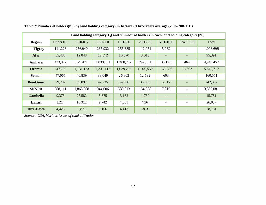
Table 2: Number of holders(Nij) by land holding category (in hectare), Three years average (2005-2007E.C)

Region

Land holding category(Li) and Number of holders in each land holding category (Nij)

Under 0.1 0.10-0.5 0.51-1.0 1.01-2.0 2.01-5.0 5.01-10.0 Over 10.0 Total

Tigray 111,228 256,940 265,932 255,685 112,951 5,962 - 1,008,698

Afar 55,486 12,848 12,572 10,870 3,615 - - 95,391

Amhara 423,972 829,471 1,039,801 1,380,232 742,391 30,126 464 4,446,457

Oromia 347,793 1,131,123 1,331,117 1,639,296 1,205,550 169,236 16,602 5,840,717

Somali 47,065 40,839 33,049 26,803 12,192 603 - 160,551

Ben-Gumz 29,797 69,097 47,735 54,306 35,900 5,517 - 242,352

SNNPR 388,111 1,868,068 944,006 530,013 154,868 7,015 - 3,892,081

Gambella 9,373 25,582 5,875 3,182 1,739 - - 45,751

Harari 1,214 10,312 9,742 4,853 716 - - 26,837

Dire-Dawa 4,428 9,871 9,166 4,413 303 - - 28,181

Source: CSA, Various issues of land utilization

18

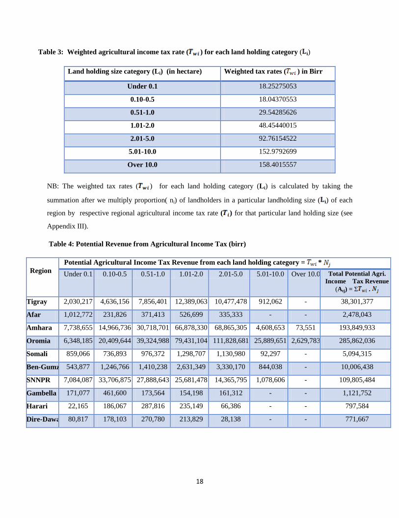
Table 3: Weighted agricultural income tax rate ( ) for each land holding category ( )

Land holding size category (Li) (in hectare) Weighted tax rates ( ) in Birr

Under 0.1 18.25275053

0.10-0.5 18.04370553

0.51-1.0 29.54285626

1.01-2.0 48.45440015

2.01-5.0 92.76154522

5.01-10.0 152.9792699

Over 10.0 158.4015557

NB: The weighted tax rates ( ) for each land holding category (Li) is calculated by taking the

summation after we multiply proportion( ni) of landholders in a particular landholding size ( ) of each

region by respective regional agricultural income tax rate ( ) for that particular land holding size (see

Appendix III).

Table 4: Potential Revenue from Agricultural Income Tax (birr)

Region

Potential Agricultural Income Tax Revenue from each land holding category = * Under 0.1 0.10-0.5 0.51-1.0 1.01-2.0 2.01-5.0 5.01-10.0 Over 10.0 Total Potential Agri.

Income Tax Revenue (Atj) = Σ .

Tigray 2,030,217 4,636,156 7,856,401 12,389,063 10,477,478 912,062 - 38,301,377

Afar 1,012,772 231,826 371,413 526,699 335,333 - - 2,478,043

Amhara 7,738,655 14,966,736 30,718,701 66,878,330 68,865,305 4,608,653 73,551 193,849,933

Oromia 6,348,185 20,409,644 39,324,988 79,431,104 111,828,681 25,889,651 2,629,783 285,862,036

Somali 859,066 736,893 976,372 1,298,707 1,130,980 92,297 - 5,094,315

Ben-Gumz 543,877 1,246,766 1,410,238 2,631,349 3,330,170 844,038 - 10,006,438

SNNPR 7,084,087 33,706,875 27,888,643 25,681,478 14,365,795 1,078,606 - 109,805,484

Gambella 171,077 461,600 173,564 154,198 161,312 - - 1,121,752

Harari 22,165 186,067 287,816 235,149 66,386 - - 797,584

Dire-Dawa 80,817 178,103 270,780 213,829 28,138 - - 771,667

19

3.5.2. Agricultural land use fee The tax base for land use tax is land holding in the same way as agricultural income tax. Hence, the

treatment of land use tax is the same as that of agricultural income tax. Land holding tax rate varies with

the land size and may differ also across regions. Since land use fee is allocated to Regional States in

accordance with the provisions of the new constitution of 1995, each Regional State uses different tax rate

depending on the holding size category. Representative tax system requires a weighted land use fee rates

( ) applicable to all regions for each land holding category. This standard tax rate is obtained by

multiplying the proportion of landholders (ni)in a particular landholding size ( ) by respective regional

land use fee rate ( ) applicable for that particular land holding category. Accordingly, the proportion of

landholders (weight) in a particular landholding size (i) in region (j) can be calculated as follows:

Let be the region j’s total number of agricultural landholders in each land size category

= ------------------------------------------------------------- (4)

Now, once the proportion of landholders in a particular landholding size ( ) of each region is known and

respective regional land use fee rate ( ) for that particular land size known, we compute the weighted

land use fee rate (Twi) as follows:

= --------------------------------------------------------------- (5)

Therefore, once we get (the weighted land use fee rate applicable to each land holding category (i) of

all regions) and (regional total number of agricultural landholders in each land holding category); we

are in a position to estimate the potential agricultural land usefee for each region as follows:

Total Potential Agricultural Land Use feeRevenue for Region j -------(6)

20

Table 5: Number of holders(Nij) by land holding category Li(in hectare), three years average (2005-2007 E.C)

Region Land holding category(L) and Number of holders in each land holding category Under 0.1 0.10-0.5 0.51-1.0 1.01-2.0 2.01-5.0 5.01-10.0 Over 10.0 Total

Tigray 111,228 256,940 265,932 255,685 112,951 5,962 - 1,008,698 Afar 55,486 12,848 12,572 10,870 3,615 - - 95,391 Amhara 423,972 829,471 1,039,801 1,380,232 742,391 30,126 464 4,446,457 Oromia 347,793 1,131,123 1,331,117 1,639,296 1,205,550 169,236 16,602 5,840,717 Somali 47,065 40,839 33,049 26,803 12,192 603 - 160,551 Ben-Gumz 29,797 69,097 47,735 54,306 35,900 5,517 - 242,352 SNNPR 388,111 1,868,068 944,006 530,013 154,868 7,015 - 3,892,081 Gambella 9,373 25,582 5,875 3,182 1,739 - - 45,751 Harari 1,214 10,312 9,742 4,853 716 - - 26,837 Dire-Dawa 4,428 9,871 9,166 4,413 303 - - 28,181 Source: CSA various issues of land utilization

21

Table 6: Weighted land use fee rate ( ) for each land holding category ( )

Land holding size category (Li) (in hectare)

Weighted tax rates ( ) in Birr

Under 0.1 11.31

0.10-0.5 11.97

0.51-1.0 17.52

1.01-2.0 26.81

2.01-5.0 53.65

5.01-10.0 109.21

Over 10.0 117.69

Table 7:Potential Agricultural Land use Tax Revenue from each land holding category = *

Region Under 0.1 0.10-0.5 0.51-1.0 1.01-2.0 2.01-5.0 5.01-10.0 Over 10.0 Total Potential Agri. Land use Tax Revenue

Tigray 1,258,368.14 3,075,985.05 4,660,074 6,855,002.39 6,060,137.95 651,141.35 - 22,560,709.01

Afar 627,735.95 153,811.02 220,306 291,428.42 193,955.46 - - 1,487,236.72

Amhara 4,796,569.73 9,930,093.06 18,220,993 37,004,501.40 39,831,459.6 3,290,218.75 54,646.16 113,128,481.58

Oromia 3,934,729.12 13,541,339.99 23,325,867 43,950,087.00 64,681,329.8 18,483,189.18 1,953,845.5 169,870,387.89

Somali 532,465.72 488,911.87 579,141 718,588.67 654,154.81 65,893.20 - 3,039,155.37

Ben-Gumz 337,105.72 827,201.15 836,492 1,455953.52 1,926,159.26 602,576.96 - 5,985,488.32

SNNPR 4,390,855.71 22,363,753.44 16,542,327 14,209,838.93 8,309,127.09 770,040.35 - 66,585,942.06

Gambella 106,036.84 306,261.28 102,951 85,319.45 93,302.50 - - 693,870.82

Harari 13,738.25 123,451.07 170,720 130,110.59 38,397.64 - - 476,417.65

Dire-Dawa 50,092.02 118,167.60 160,615 118,314.04 16,274.73 - - 463,463.26

22

3.5.3. Payroll tax

One of the tax sources assigned to regional States in the Constitution is payroll tax from employees of the

States, NGOs, and private organizations. In order to estimate the potential regional revenue obtained from

overall payroll tax we used the actual payroll tax revenue collected from government and NGOs

employees in each year (RGNt) and the actual number of private employees (EPit) under specified salary

categories(i) for the three years and the corresponding tax (trpi) per worker.The overall payroll tax

revenue per region is calculated as follows:

The Average Total Payroll Tax Revenue = [RGNt+ )]/3 ……………………..(7)

where i represents the salary rangeand t represents time period (three years)

Private employees are those employed in large and medium scale manufacturing industries, small scale

manufacturing industries, and distributive trade and other services.Estimation of potential payroll tax

from employees of government and NGO, and from employees of private organizations in large and

medium scale manufacturing industries, small scale manufacturing industries, and distributive trade and

other services is carried out in slightly different ways.

For employees of government and NGOs, the potential payroll tax is approximated by the actual payroll

tax revenue regions have collected at the applicable tax rate. This is because all employees that have to

pay income tax actually pay the taxes according to income tax law; and there is no way to escape the tax

payment. This revenue is computed as an average tax of three years period.

Table 8: Total potential PayrollTax in Government and NGO employment Region Total potential Payroll Tax in Government and NGO employment

Tigray 712,310,745.3 10.3% Afar 142,497,125.4 2.1% Amhara 1,370,006,502.5 19.7% Oromia 2,460,865,891.1 35.4% Somalia 198,100,367.6 2.9% Benishangul 141,255,623.0 2.0% S.N.N.P.R 1,686,168,989.6 24.3% Gambela 77,205,182.8 1.1% Harari 62,766,385.3 0.9% Dire Dawa 90,970,149.5 1.3%

6,942,146,962.10

100%

23

In order to estimate the potential payroll tax of each region from private organizations, the numbers of

employees in different private organizations with in the region are used as potential tax base. This is

because the collection of taxes from private organizations entails tax effort. The corresponding tax rate is

computed on the basis of three years average regional wage derived from the CSA data on wages and

salaries. Applying the tax rate on the number of private organizations’ employees gives the potential tax

that could be collected from private employees.

For all employees of business organizations (i.e., LMSMI, SSMI, Distributive trade and other services

operating in each region), for which data are available from CSA, we compute the potential tax revenue

by: generating a single tax rate, which is a weighted average tax rate to be applied for all regions, and

using the total salaries and wages per region. The weighted average tax rate is a representative tax rate

that reflects the contributions of the various tax rates applicable to various income brackets in the salary

scales and that takes into consideration the proportions of taxpayers falling in the progressive tax brackets

pertaining to the salary scales in all regions together

Table 9a: An example from LMSMI in 2012 Salary range

1.Upper side of the salary bracket 200 400 600 800 1200 1600 2000 3145 2.Total number of employees in all regions(within the bracket)

577 6802 20070 21581 21711 11497 6957 17856 107051

3.Percentage of workers (within salary bracket in all employees)(column in 3 above divided by 107051 )

1% 6% 19% 20% 20% 11% 6% 17%

4.Applicable tax rate (for the salary bracket)

0% 0% 10% 10% 10% 10% 15% 15%

5.Taxable part of salary (corresponding to the tax rate)

15 215 615 1015 350 2560

6.Tax Revenue (from the salary bracket)

0 1.5 21.5 61.5 101.5 159 330.75

7.Tax collected as a percentage of theupper side of salary bracket

0.0% 0.0% 0.3% 2.7% 5.1% 6.3% 8.0% 10.5%

8.Weighted tax rate 0.0% 0.0% 0.0% 0.5% 1.0% 0.7% 0.5% 1.8% 4.6%

24

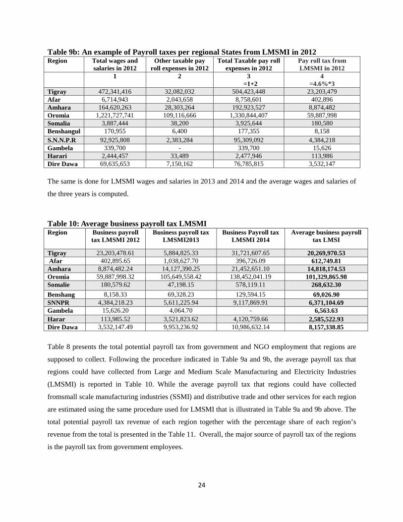
Table 9b: An example of Payroll taxes per regional States from LMSMI in 2012 Region Total wages and

salaries in 2012 Other taxable pay

roll expenses in 2012 Total Taxable pay roll

expenses in 2012 Pay roll tax from LMSMI in 2012

1 2 3 =1+2

4 =4.6%*3

Tigray 472,341,416 32,082,032 504,423,448 23,203,479 Afar 6,714,943 2,043,658 8,758,601 402,896 Amhara 164,620,263 28,303,264 192,923,527 8,874,482 Oromia 1,221,727,741 109,116,666 1,330,844,407 59,887,998 Somalia 3,887,444 38,200 3,925,644 180,580 Benshangul 170,955 6,400 177,355 8,158 S.N.N.P.R 92,925,808 2,383,284 95,309,092 4,384,218 Gambela 339,700 - 339,700 15,626 Harari 2,444,457 33,489 2,477,946 113,986 Dire Dawa 69,635,653 7,150,162 76,785,815 3,532,147

The same is done for LMSMI wages and salaries in 2013 and 2014 and the average wages and salaries of

the three years is computed.

Table 10: Average business payroll tax LMSMI Region Business payroll

tax LMSMI 2012 Business payroll tax

LMSMI2013 Business Payroll tax

LMSMI 2014 Average business payroll

tax LMSI

Tigray 23,203,478.61 5,884,825.33 31,721,607.65 20,269,970.53 Afar 402,895.65 1,038,627.70 396,726.09 612,749.81 Amhara 8,874,482.24 14,127,390.25 21,452,651.10 14,818,174.53 Oromia 59,887,998.32 105,649,558.42 138,452,041.19 101,329,865.98 Somalie 180,579.62 47,198.15 578,119.11 268,632.30 Benshang 8,158.33 69,328.23 129,594.15 69,026.90 SNNPR 4,384,218.23 5,611,225.94 9,117,869.91 6,371,104.69 Gambela 15,626.20 4,064.70 - 6,563.63 Harar 113,985.52 3,521,823.62 4,120,759.66 2,585,522.93 Dire Dawa 3,532,147.49 9,953,236.92 10,986,632.14 8,157,338.85

Table 8 presents the total potential payroll tax from government and NGO employment that regions are

supposed to collect. Following the procedure indicated in Table 9a and 9b, the average payroll tax that

regions could have collected from Large and Medium Scale Manufacturing and Electricity Industries

(LMSMI) is reported in Table 10. While the average payroll tax that regions could have collected

fromsmall scale manufacturing industries (SSMI) and distributive trade and other services for each region

are estimated using the same procedure used for LMSMI that is illustrated in Table 9a and 9b above. The

total potential payroll tax revenue of each region together with the percentage share of each region’s

revenue from the total is presented in the Table 11. Overall, the major source of payroll tax of the regions

is the payroll tax from government employees.

25

Table 11: Total Payroll Tax (Tax from wages and salaries) by business type Region Payroll tax

from LMSI Payroll tax

from SSMI

Payroll tax from

SERVICE

Total potential payroll tax in

Government&NGO employment

Total Potential

payroll tax revenue

Percentage in total

Tigray 20,269,971 0 - 712,310,745.3 732,580,716 10.3% Afar 612,750 0 66,254 142,497,125.4 143,176,129 2.0%

Amhara 14,818,175 0 85,259 1,370,006,502.5 1,384,909,936 19.5% Oromia 101,329,866 0 108,626 2,460,865,891.1 2,562,304,383 36.1% Somalia 268,632 78,230 - 198,100,367.6 198,447,230 2.8%

Benshangul 69,027 0 - 141,255,623.0 141,324,650 2.0% S.N.N.P.R 6,371,105 0 451,638 1,686,168,989.6 1,692,991,732 23.9% Gambela 6,564 0 - 77,205,182.8 77,211,746 1.1% Harari 2,585,523 0 - 62,766,385.3 65,351,908 0.9%

Dire Dawa 8,157,339 123895.2 698,742 90,970,149.5 99,950,125 1.4% Total 154,488,952 202125.2 1410519 6,942,146,962.1 7,098,248,555

2.18% 0.003% 0.02% 97.80% 100% 100% Source CSA employment and unemployment survey (Raw data on average regional wage is derived from CSA and the corresponding tax rate is applied on the basis of income tax law.) 3.5.4. Turnover tax (TOT)

Turnover Tax applies to goods and services sold locally by tax payers who are not registered for Value

Added Tax (VAT). The tax base for Turnover Tax is sales revenue of establishments in industrial and

service sectors operating in the regions with annual sales below 500,000 Birr. Virtually all TOT paid by

firms is by those engaged in the distributivetrade sector and small scale manufacturing sectors within the

regions and are collected by the regional revenue authorities. CSA dataset on small scale manufacturing ,

distributive trade and other service surveys will be used to calculate TOT.

Accordingly, in order to estimate the potential revenue from TOT, we multiplied regional sales revenue

(RSit) of non-VAT collecting businesses (manufacturers, wholesalers, retailer and Vehicle repair) for

three years by the respective TOT rate (tot) as shown in the following formula. Then, the three-year

average potential Turnover Tax is calculated and presented in the table that follows. The applicable TOT

rule is uniform across regions and applicable sales tax rate is 2% for manufacturing; 2% for distributive

trade services and 10% for other services (Ethiopian Legal Brief, 2011).

Therefore, the potential turnover tax revenue is calculated as follows:

Total Potential Revenue from Turnover Tax it = …………………(8)

26

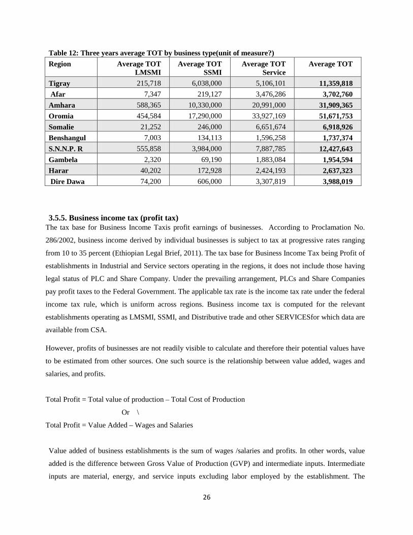
Table 12: Three years average TOT by business type(unit of measure?) Region Average TOT

LMSMI Average TOT

SSMI Average TOT

Service Average TOT

Tigray 215,718 6,038,000 5,106,101 11,359,818 Afar 7,347 219,127 3,476,286 3,702,760 Amhara 588,365 10,330,000 20,991,000 31,909,365 Oromia 454,584 17,290,000 33,927,169 51,671,753 Somalie 21,252 246,000 6,651,674 6,918,926 Benshangul 7,003 134,113 1,596,258 1,737,374 S.N.N.P. R 555,858 3,984,000 7,887,785 12,427,643 Gambela 2,320 69,190 1,883,084 1,954,594 Harar 40,202 172,928 2,424,193 2,637,323 Dire Dawa 74,200 606,000 3,307,819 3,988,019

3.5.5. Business income tax (profit tax) The tax base for Business Income Taxis profit earnings of businesses. According to Proclamation No.

286/2002, business income derived by individual businesses is subject to tax at progressive rates ranging

from 10 to 35 percent (Ethiopian Legal Brief, 2011). The tax base for Business Income Tax being Profit of

establishments in Industrial and Service sectors operating in the regions, it does not include those having

legal status of PLC and Share Company. Under the prevailing arrangement, PLCs and Share Companies

pay profit taxes to the Federal Government. The applicable tax rate is the income tax rate under the federal

income tax rule, which is uniform across regions. Business income tax is computed for the relevant

establishments operating as LMSMI, SSMI, and Distributive trade and other SERVICESfor which data are

available from CSA.

However, profits of businesses are not readily visible to calculate and therefore their potential values have

to be estimated from other sources. One such source is the relationship between value added, wages and

salaries, and profits.

Total Profit = Total value of production – Total Cost of Production

Or \

Total Profit = Value Added – Wages and Salaries

Value added of business establishments is the sum of wages /salaries and profits. In other words, value

added is the difference between Gross Value of Production (GVP) and intermediate inputs. Intermediate

inputs are material, energy, and service inputs excluding labor employed by the establishment. The

27

surplus over the value of intermediate inputs is the Value Added thatconstitutes wages and salaries and

profits, which are factor incomes. If value added and wages and salaries are known, profit can be known

as a difference of the two.

Value added and wages and salaries of establishments in industrial and service business providers located

in each region will be used to calculate the business income tax. In order to estimate regional potential

revenue obtained from profit tax, we will take in to account the following variables:

i. Value added at factor cost (VAijt) in industrial business (i) region (j) and year (t) and the

corresponding wages and salaries (SWijt). The index (i) of the business type refers to business

income category implying the applicable standard tax rate.

ii. Value added in services (VAsjt) in service (s) region (j) and year (t) and the corresponding wages

and salaries (SWijt).The index (s) of the business type refers to business income category

implying the applicable standard tax rate.

iii. The standard Profit tax rate (ti) is applicable to industrial businesses of tax category (i)

iv. The standard Profit tax rate (ts) is applicable to service businesses of tax category (s).

It is important to note that although they are operating in a particular region, they may not pay profit tax

to the region by virtue of being federal taxpayers. These groups of taxpayers have to be excluded with the

use of identifiers such as their legal status.

The potential profit (Pijt) that is taxable in category (i) in year (t) and in region j is:

Pijt= (VAijt-SWijt) ………………………………………………………………………(9)

The potential profit (Pst) in services that is taxable in category (s) in year (t) and in region j is:

Psjt=(VAsjt-SWsjt) …………………………………………………………………..( 10)

Since Pijt andPsjt (business profits in year t from the respective business categories) fluctuate from year to

year, to get a figure representative of the near past, the average of the latest three years is taken.

Pij= (ΣPijt)/3 andPsj = (ΣPsjt)/3……………………………………………………(11)

We compute the potential Business Income Tax Revenue by using the total computed profits per region in

each of the sectors and generating a single tax rate, which is a weighted average tax rate to be applied for

all regions. The weighted average tax rate varies with total profit. The greater the total profit is the greater

will be the average weighted tax rate approaching to the highest tax rate i.e.35%. Total profits are

computed per region from total value of production and total costs of production of relevant

establishments. Designating ti for the weighted tax rate applicable to all income categories, the total

potential industry profit tax (TIj) from all profit categories in region (j) is:

28

TIj = Σ(Pij. ti) …………………………………………………………………………(12)

The potential tax revenue (TSj) for region (j) in service is:

TSj = Σ(Psj .ts )………………………………………………………………………(13)

The total potential profit tax revenue(PTRj) in region(j) is :

PTRj =TIj +TSj …………………………………………………………………(14)

We compute the average profit per establishment from the total profit and the total number of

establishments of all regions together. The average profit per establishment guides us to fix which

AVERAGE WEIGHTED PROFIT TAX to use for all regions in a particular year. The weighted average

tax rate is a representative tax rate that reflects the contributions of the various income tax rates applicable

to various profit income brackets and that takes into consideration the proportions of profit falling in the

progressive tax brackets pertaining to the income scales in all regions together.

Table 13: Weighted income Taxcomputation given the average annual profit income per establishment

Average annual profit income per establishment 2,000,000

Monthly income(= 2000000/12) 166,667

Monthly Income scales 585 1,650 3,145 5,195 7,758 10,833 166,667

Maximum applicable tax rate - 0.10 0.15 0.20 0.25 0.30 0.35

Taxable income under each tax rate 1,065 1,495 2,050 2,563 3,075 155,834

Monthly Tax from monthly profit - 106.5 224.3 410.0 640.8 922.5 54,541.8 56,845.8

Weighted income Tax=Total monthly Tax /Monthly Income 0.3411

The sources of data for these computations are the large and medium scale manufacturing survey

(LMSMIS), small scale manufacturing survey (SMMIS), and distributive services survey of CSA. As in

the example shown above, using the average weighted profit tax rate as a representative tax rate, which is

estimated to be 34.1%, we compute the profit tax.Accordingly, the average profit tax for LMSMI is

computed as follows:

29

Table 14: Average Region al profit tax from LMSMI

Region Profit tax 2012 Profit Tax2013 Profit Tax 2014 Average profit tax

Tigray 68,390,917 105,006,294 95,718,426 89,705,212

Afar 27,703 3,602,481 759,629 1,463,271

Amhara 50,294,844 96,242,639 106,299,979 84,279,154

Oromia 263,451,099 631,577,000 1,116,247,128 670,425,076

Somale 13,802,952 31,760,455 34,924,733 26,829,380

Benishangul 141,581 2,043,858 5,896,936 2,694,125

S.N.N.P.R 251,208,973 109,486,197 157,202,500 172,632,557

Gambela - - - -

Harar 3,712,646 1,542,736 2,787,404 2,680,929

Diredawa 2,932,593 827,381 200,830,666 68,196,880

We follow similar procedures in computing the representative tax rate for the various services categorized

as TOT and VAT payer service establishments. The computed tax revenue on the basis of the

representative tax in the respective service categories are tabulated hereunder (refer the appendix section

for the details)

Table 15: Profit Tax from Services Total potential profit tax revenue from service establishments

Regions that pay TOT that pay VAT All

Tigray 16,474,279 220,040,000 236,514,279

Afar 10,109,962 51,300,000 61,409,962

Amhara 56,107,567 668,915,125 725,022,691

Oromia 206,912,274 600,814,465 807,726,739

Somalia 3,250,474 120,951,515 124,201,989

Benshangul 4,791,637 10,557,000 15,348,637

S.N.N.P.R 20,225,464 352,691,081 372,916,544

Gambela 5,184,307 44,507,549 49,691,856

Harari 6,310,259 42,777,000 49,087,259

Dire Dawa 3,174,966 181,710,000 184,884,966

30

Applying the same procedure for Small Scale Manufacturing Industrial establishments the representative

tax rate becomes 20% and the potential profit tax would be as follows.

Table 16: Profit tax SSMI

Region Two Years Average Profit Profit tax at representative tax rate of 20%

Tigray 196,320,359 39,264,071.7

Afar 18,081,734 3,616,346.8

Amhara 241,288,188 48,257,637.5

Oromia 163,950,000 32,790,000.0

Somalie 8,662,166 1,732,433.2

Benshangul 10,172,703 2,034,540.5

S.N.N.P.R 33,950,000 6,790,000.0

Gambela 6,588,815 1,317,763.0

Harari 4,539,607 907,921.4

Dire dawa 519,375 103,874.9

The total potential profit tax from Manufacturing and Services from the respective region is computed

and summarized as follows:

Table 17: POTENTIAL PROFIT TAX TOTAL Region LMSMI SERVICES SSMI Total

Tigray 89,705,212 236,514,279 39,264,072 365,483,563

Afar 1,463,271 61,409,962 3,616,347 66,489,579

Amhara 84,279,154 725,022,691 48,257,638 857,559,483

Oromia 670,425,076 807,726,739 32,790,000 1,510,941,815

Somalie 26,829,380 124,201,989 1,732,433 152,763,802

Benshangul 2,694,125 15,348,637 2,034,541 20,077,302

S.N.N.P.R. 172,632,557 372,916,544 6,790,000 552,339,101

Gambela - 49,691,856 1,317,763 51,009,619

Harari 2,680,929 49,087,259 907,921 52,676,109

Dire dawa 68,196,880 184,884,966 103,875 253,185,721

3.5.6. Value added tax (VAT)

31

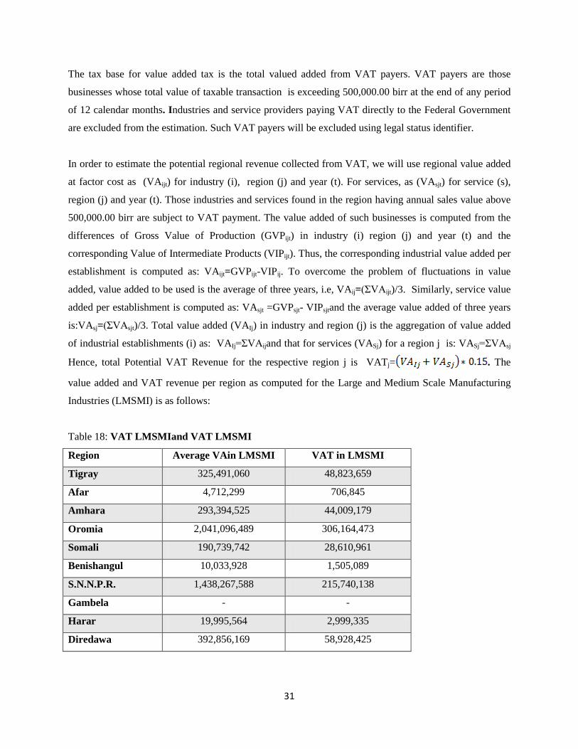
The tax base for value added tax is the total valued added from VAT payers. VAT payers are those

businesses whose total value of taxable transaction is exceeding 500,000.00 birr at the end of any period

of 12 calendar months. Industries and service providers paying VAT directly to the Federal Government

are excluded from the estimation. Such VAT payers will be excluded using legal status identifier.

In order to estimate the potential regional revenue collected from VAT, we will use regional value added

at factor cost as (VAijt) for industry (i), region (j) and year (t). For services, as (VAsjt) for service (s),

region (j) and year (t). Those industries and services found in the region having annual sales value above

500,000.00 birr are subject to VAT payment. The value added of such businesses is computed from the

differences of Gross Value of Production (GVPijt) in industry (i) region (j) and year (t) and the

corresponding Value of Intermediate Products (VIPijt). Thus, the corresponding industrial value added per

establishment is computed as: VAijt=GVPijt-VIPij. To overcome the problem of fluctuations in value

added, value added to be used is the average of three years, i.e, VAij=(ΣVAijt)/3. Similarly, service value

added per establishment is computed as: VAsjt =GVPsjt- VIPsjtand the average value added of three years

is:VAsj=(ΣVAsjt)/3. Total value added (VAIj) in industry and region (j) is the aggregation of value added

of industrial establishments (i) as: VAIj=ΣVAijand that for services (VASj) for a region j is: VASj=ΣVAsj

Hence, total Potential VAT Revenue for the respective region j is VATj= . The

value added and VAT revenue per region as computed for the Large and Medium Scale Manufacturing

Industries (LMSMI) is as follows:

Table 18: VAT LMSMIand VAT LMSMI

Region Average VAin LMSMI VAT in LMSMI

Tigray 325,491,060 48,823,659

Afar 4,712,299 706,845

Amhara 293,394,525 44,009,179

Oromia 2,041,096,489 306,164,473

Somali 190,739,742 28,610,961

Benishangul 10,033,928 1,505,089

S.N.N.P.R. 1,438,267,588 215,740,138

Gambela - -

Harar 19,995,564 2,999,335

Diredawa 392,856,169 58,928,425

32

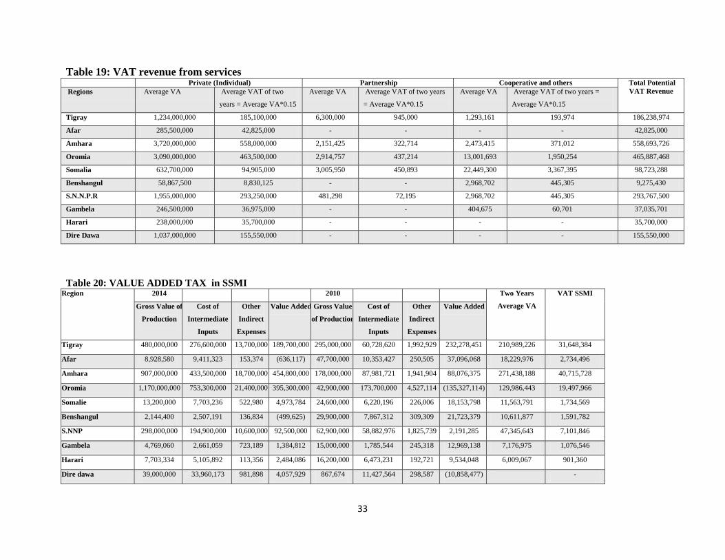
The value added(VA)and the valued added tax(VAT) that is potentially collectablefrom services

categorized by their legal status as private (individual), partnership and cooperatives and for Small Scale

ManufacturingIndustries are tabulated as follows:

33

Table 19: VAT revenue from services Private (Individual) Partnership Cooperative and others Total Potential

VAT Revenue Regions Average VA Average VAT of two

years = Average VA*0.15

Average VA Average VAT of two years

= Average VA*0.15

Average VA Average VAT of two years =

Average VA*0.15

Tigray 1,234,000,000 185,100,000 6,300,000 945,000 1,293,161 193,974 186,238,974

Afar 285,500,000 42,825,000 - - - - 42,825,000

Amhara 3,720,000,000 558,000,000 2,151,425 322,714 2,473,415 371,012 558,693,726

Oromia 3,090,000,000 463,500,000 2,914,757 437,214 13,001,693 1,950,254 465,887,468

Somalia 632,700,000 94,905,000 3,005,950 450,893 22,449,300 3,367,395 98,723,288

Benshangul 58,867,500 8,830,125 - - 2,968,702 445,305 9,275,430

S.N.N.P.R 1,955,000,000 293,250,000 481,298 72,195 2,968,702 445,305 293,767,500

Gambela 246,500,000 36,975,000 - - 404,675 60,701 37,035,701

Harari 238,000,000 35,700,000 - - - - 35,700,000

Dire Dawa 1,037,000,000 155,550,000 - - - - 155,550,000

Table 20: VALUE ADDED TAX in SSMI Region 2014 2010 Two Years

Average VA

VAT SSMI

Gross Value of

Production

Cost of

Intermediate

Inputs

Other

Indirect

Expenses

Value Added Gross Value

of Production

Cost of

Intermediate

Inputs

Other

Indirect

Expenses

Value Added

Tigray 480,000,000 276,600,000 13,700,000 189,700,000 295,000,000 60,728,620 1,992,929 232,278,451 210,989,226 31,648,384

Afar 8,928,580 9,411,323 153,374 (636,117) 47,700,000 10,353,427 250,505 37,096,068 18,229,976 2,734,496

Amhara 907,000,000 433,500,000 18,700,000 454,800,000 178,000,000 87,981,721 1,941,904 88,076,375 271,438,188 40,715,728

Oromia 1,170,000,000 753,300,000 21,400,000 395,300,000 42,900,000 173,700,000 4,527,114 (135,327,114) 129,986,443 19,497,966

Somalie 13,200,000 7,703,236 522,980 4,973,784 24,600,000 6,220,196 226,006 18,153,798 11,563,791 1,734,569

Benshangul 2,144,400 2,507,191 136,834 (499,625) 29,900,000 7,867,312 309,309 21,723,379 10,611,877 1,591,782

S.NNP 298,000,000 194,900,000 10,600,000 92,500,000 62,900,000 58,882,976 1,825,739 2,191,285 47,345,643 7,101,846

Gambela 4,769,060 2,661,059 723,189 1,384,812 15,000,000 1,785,544 245,318 12,969,138 7,176,975 1,076,546

Harari 7,703,334 5,105,892 113,356 2,484,086 16,200,000 6,473,231 192,721 9,534,048 6,009,067 901,360

Dire dawa 39,000,000 33,960,173 981,898 4,057,929 867,674 11,427,564 298,587 (10,858,477) -

34

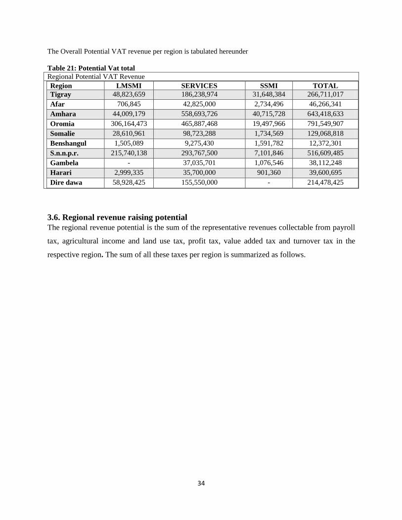
The Overall Potential VAT revenue per region is tabulated hereunder Table 21: Potential Vat total Regional Potential VAT Revenue

Region LMSMI SERVICES SSMI TOTAL Tigray 48,823,659 186,238,974 31,648,384 266,711,017 Afar 706,845 42,825,000 2,734,496 46,266,341 Amhara 44,009,179 558,693,726 40,715,728 643,418,633 Oromia 306,164,473 465,887,468 19,497,966 791,549,907 Somalie 28,610,961 98,723,288 1,734,569 129,068,818 Benshangul 1,505,089 9,275,430 1,591,782 12,372,301 S.n.n.p.r. 215,740,138 293,767,500 7,101,846 516,609,485 Gambela - 37,035,701 1,076,546 38,112,248 Harari 2,999,335 35,700,000 901,360 39,600,695 Dire dawa 58,928,425 155,550,000 - 214,478,425

3.6. Regional revenue raising potential The regional revenue potential is the sum of the representative revenues collectable from payroll

tax, agricultural income and land use tax, profit tax, value added tax and turnover tax in the

respective region. The sum of all these taxes per region is summarized as follows.

35

Table 22: Summary of regional revenue potential Region Total Potential

pay roll tax revenue

Total potential agri. income tax

Total land use fee Potential Profit Tax

Potential TOT Potential VAT Total regional Revenue Potential

Tigray 732,580,716 38,301,377 22,560,709 365,483,563 11,359,818.47 266,711,016.93 1,436,997,201

Afar 143,176,129 2,478,043 1,487,237 66,489,579 3,702,759.74 46,266,341.13 263,600,089

Amhara 1,384,909,936 193,849,933 113,128,482 857,559,483 31,909,364.99 643,418,632.85 3,224,775,831

Oromia 2,562,304,383 285,862,036 169,870,388 1,510,941,815 51,671,753.14 791,549,907.30 5,372,200,282

Somalie 198,447,230 5,094,315 3,039,155 152,763,802 6,918,926.45 129,068,817.50 495,332,246

Benshangul 141,324,650 10,006,438 5,985,488 20,077,302 1,737,374.22 12,372,301.00 191,503,554

S.n.n.p.r. 1,692,991,732 109,805,484 66,585,942 552,339,101 12,427,642.89 516,609,484.63 2,950,759,387

Gambela 77,211,746 1,121,752 693,871 51,009,619 1,954,593.96 38,112,247.50 170,103,829

Harari 65,351,908 797,584 476,418 52,676,109 2,637,322.98 39,600,694.70 161,540,036

Dire dawa 99,950,125 771,667 463,463 253,185,721 3,988,018.78 214,478,425.30 572,837,421

Total 14,839,649,876

36

3.7. Total regional revenue potential

The total revenue potential of regions is composed of their computed potential revenue raising

capacity and the shared revenues with the Federal government. Summing up the potential

revenue generated by regions and the revenues to be shared with the federal Government

constitute the total potential regional revenue as tabulated hereunder.

Table 23: Total potential revenue Region Potential Revenue

generated by the Regions alone

Revenues Shared with Federal Government

Total Potential Revenue

Percentage in total potential revenue

Tigray 1,436,997,201 314,927,121 1,751,924,322 11.0%

Afar 263,600,089 2,116,753 265,716,842 1.7%

Amhara 3,224,775,831 251,301,023 3,476,076,854 21.9%

Oromia 5,372,200,282 398,157,768 5,770,358,051 36.3%

Somale 495,332,246 122,705 495,454,952 3.1%

Benshangul 191,503,554 346,990 191,850,544 1.2%

S.N.N.P.R 2,950,759,387 45,351,703 2,996,111,090 18.8%

Gambela 170,103,829 7,141,986 177,245,815 1.1%

Harari 161,540,036 38,148,182 199,688,218 1.3%

Dire Dawa 572,837,421 572,837,421 3.6%

Total 14,839,649,876 1,057,614,232 15,897,264,107

37

Appendices Total Potential Value Added Tax Revenue(in Birr ) (Only for VAT payer services )

Region Private (Individual) Partnership Cooperatives and others

2,011 2,014 Total VA Average VA=( Total VA/2)

Average VAT of two years

2,011 2,014 Total VA Average VA =(Total VA/2)

Average VAT of two

years

2,011 2,014 Total VA Average VA= (Total

VA/2)

Average VA*0.15

Total Potential

VAT Revenue

Tigray 618,000,000 1,850,000,000 2,468,000,000 1,234,000,000 185,100,000 12,600,000 12,600,000 6,300,000 945,000 2,586,322 2,586,322 1,293,161 193,974 186,238,974

Afar 267,000,000 304,000,000 571,000,000 285,500,000 42,825,000 - - - - - - - 42,825,000

Amhara 3,230,000,000 4,210,000,000 7,440,000,000 3,720,000,000 558,000,000 4,302,850 4,302,850 2,151,425 322,714 4,946,829

- 4,946,829 2,473,415 371,012 558,693,726

Oromia 3,540,000,000 2,640,000,000 6,180,000,000 3,090,000,000 463,500,000 5,829,514 5,829,514 2,914,757 437,214 26,003,386 26,003,386 13,001,693 1,950,254 465,887,468

Somalia 95,400,000 1,170,000,000 1,265,400,000 632,700,000 94,905,000 4,931,300

1,080,600 6,011,900 3,005,950 450,893 44,898,600 44,898,600 22,449,300 3,367,395 98,723,288

Benshangul 67,335,000 50,400,000 117,735,000 58,867,500 8,830,125 - - - 5,937,404 5,937,404 2,968,702 445,305 9,275,430

S.N.N.P.R 1,050,000,000 2,860,000,000 3,910,000,000 1,955,000,000 293,250,000 962,596 962,596 481,298 72,195 5,937,404 5,937,404 2,968,702 445,305 293,767,500

Gambela 385,000,000 108,000,000 493,000,000 246,500,000 36,975,000 - - - 809,350 809,350 404,675 60,701 37,035,701

Harari 420,000,000 56,000,000 476,000,000 238,000,000 35,700,000 - - - - - - 35,700,000

Dire Dawa 754,000,000 1,320,000,000 2,074,000,000 1,037,000,000 155,550,000 - - - - - - 155,550,000

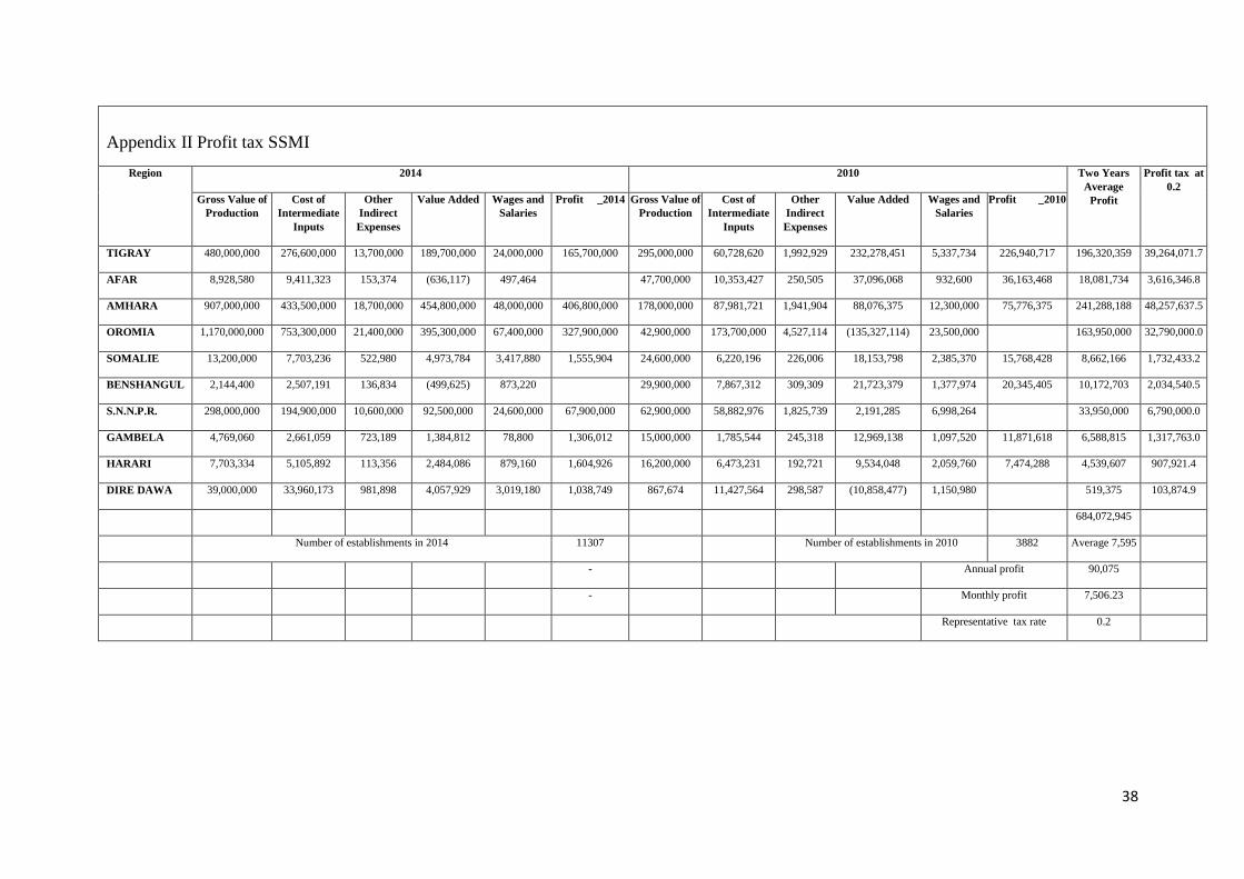
38

Appendix II Profit tax SSMI

Region 2014 2010 Two Years Average

Profit

Profit tax at 0.2

Gross Value of Production

Cost of Intermediate

Inputs

Other Indirect Expenses

Value Added Wages and Salaries

Profit _2014 Gross Value of Production

Cost of Intermediate

Inputs

Other Indirect Expenses

Value Added Wages and Salaries

Profit _2010

TIGRAY 480,000,000 276,600,000 13,700,000 189,700,000 24,000,000 165,700,000 295,000,000 60,728,620 1,992,929 232,278,451 5,337,734 226,940,717 196,320,359 39,264,071.7

AFAR 8,928,580 9,411,323 153,374 (636,117) 497,464 47,700,000 10,353,427 250,505 37,096,068 932,600 36,163,468 18,081,734 3,616,346.8

AMHARA 907,000,000 433,500,000 18,700,000 454,800,000 48,000,000 406,800,000 178,000,000 87,981,721 1,941,904 88,076,375 12,300,000 75,776,375 241,288,188 48,257,637.5

OROMIA 1,170,000,000 753,300,000 21,400,000 395,300,000 67,400,000 327,900,000 42,900,000 173,700,000 4,527,114 (135,327,114) 23,500,000 163,950,000 32,790,000.0

SOMALIE 13,200,000 7,703,236 522,980 4,973,784 3,417,880 1,555,904 24,600,000 6,220,196 226,006 18,153,798 2,385,370 15,768,428 8,662,166 1,732,433.2

BENSHANGUL 2,144,400 2,507,191 136,834 (499,625) 873,220 29,900,000 7,867,312 309,309 21,723,379 1,377,974 20,345,405 10,172,703 2,034,540.5

S.N.N.P.R. 298,000,000 194,900,000 10,600,000 92,500,000 24,600,000 67,900,000 62,900,000 58,882,976 1,825,739 2,191,285 6,998,264 33,950,000 6,790,000.0

GAMBELA 4,769,060 2,661,059 723,189 1,384,812 78,800 1,306,012 15,000,000 1,785,544 245,318 12,969,138 1,097,520 11,871,618 6,588,815 1,317,763.0

HARARI 7,703,334 5,105,892 113,356 2,484,086 879,160 1,604,926 16,200,000 6,473,231 192,721 9,534,048 2,059,760 7,474,288 4,539,607 907,921.4

DIRE DAWA 39,000,000 33,960,173 981,898 4,057,929 3,019,180 1,038,749 867,674 11,427,564 298,587 (10,858,477) 1,150,980 519,375 103,874.9

684,072,945

Number of establishments in 2014 11307 Number of establishments in 2010 3882 Average 7,595

- Annual profit 90,075

- Monthly profit 7,506.23

Representative tax rate 0.2

39

Appendix III Agricultural income tax rates

Reg

ions

und

er 0

.10

Wei

ght

Agr

i-inc

ome

tax

wei

ghte

d t

0.1

0-0.

5

Wei

ght

Agr

i-inc

ome

tax

wei

ghte

d av

erag

e ta

x

0.5

1-1.

0

Wei

ght

Agr

i-inc

ome

tax

wei

ghte

d av

erag

e ta

x

1.0

1-2.

0

Wei

ght

Agr

i-inc

ome

tax

w

eigh

ted

aver

age

tax

2

.01-

5.0

Wei

ght

Agr

i-inc

ome

tax

wei

ghte

d av

erag

e ta

x

5.0

1-10

.0

Wei

ght

Agr

i-inc

ome

tax

w

eigh

ted

aver

age

tax

o

ver

10

Wei

ght

Agr

i-inc

ome

tax

w

eigh

ted

aver

age

tax

Tigray 111,228 0.08 - - 256,940 0.06 10.00 0.60 265,932 0.07 20.00 1.44 255,685 0.07 35.00 2.29 112,951 0.05 81.67 4.06 5,962 0.03 175.00 4.78 205.00 -

Afar 55,486 0.04 20.00 0.78 12,848 0.00 20.00 0.06 12,572 0.00 30.00 0.10 10,870 0.00 47.50 0.13 3,615 0.00 120.00 0.19 - - -

Amhara 423,972 0.30 22.50 6.73 829,471 0.19 22.50 4.39 1,039,801 0.28 32.50 9.14 1,380,232 0.35 53.75 18.98 742,391 0.33 101.25 33.11 30,126 0.14 101.25 13.96 464 0.03 101.25 2.75

Oromia 347,793 0.25 30.00 7.36 1,131,123 0.27 30.00 7.98 1,331,117 0.36 40.00 14.39 1,639,296 0.42 55.00 23.06 1,205,550 0.53 95.00 50.45 169,236 0.77 160.00 123.93 16,602 0.97 160.00 155.65

Somali 47,065 0.03 - 40,839 0.01 - 33,049 0.01 - 26,803 0.01 - 12,192 0.01 - 603 0.00 - - -

Ben-Gumz

29,797 0.02 17.60 0.37 69,097 0.02 17.60 0.29 47,735 0.01 35.20 0.45 54,306 0.01 59.70 0.83 35,900 0.02 130.08 2.06 5,517 0.03 280.08 7.07 - -

SNNPR 388,111 0.27 10.25 2.80 1,868,068 0.44 10.25 4.50 944,006 0.26 15.25 3.89 530,013 0.14 22.75 3.08 154,868 0.07 41.50 2.83 7,051 0.03 100.50 3.24 - 160.00 -

Gambella 9,373 0.01 30.00 0.20 25,582 0.01 30.00 0.18 5,875 0.00 30.00 0.05 3,182 0.00 30.00 0.02 1,739 0.00 30.00 0.02 - - - -

Harari 1,214 0.00 20.00 0.02 10,312 0.00 20.00 0.05 9,742 0.00 30.00 0.08 4,853 0.00 47.50 0.06 716 0.00 123.30 0.04 - - - -

Diredawa 4,428 0.00 9,871 0.00 9,166 0.00 4,413 0.00 303 0.00 -

All Regions

1,418,467 4,254,152 3,698,996 3,909,653 2,270,225 218,496 17,066

weighted average tax rates

18.25 18.04 29.54 48.45 92.76 152.98 158.40

40

Appendix IV Weights land use tax

Reg

ions

und

er 0

.10

Wei

ght

land

use

fee

wei

ghte

d av

erag

e fe

e in

0.1

0-0.

5

Wei

ght

land

use

fee

wei

ghte

d av

erag

e fe

e in

0.5

1-1.

0

Wei

ght

land

use

fee

wei

ghte

d av

erag

e fe

e in

1.0

1-2.

0

Wei

ght

land

use

fee

wei

ghte

d av

erag

e fe

e in

2.0

1-5.

0

Wei

ght

land

use

fee

wei

ghte

d av

erag

e fe

e in

5.0

1-10

.0

Wei

ght

land

use

fee

wei

ghte

d av

erag

e fe

e in

ove

r 10

Wei

ght

land

use

fee

wei

ghte

d av

erag

e fe

e in

Tigray 111,228 0.08 - - 256,940 0.06 10.00 0.60 265,932 0.07 15.00 1.08 255,685 0.07 25.00 1.63 112,951 0.05 61.67 3.07 5,962 0.03 132.50 3.62 162.50 -

Afar 55,486 0.04 15.00 0.59 12,848 0.00 20.00 0.06 12,572 0.00 25.00 0.08 10,870 0.00 30.00 0.08 3,615 0.00 49.20 0.08 - - -

Amhara 423,972 0.30 12.50 3.74 829,471 0.19 12.50 2.44 1,039,801 0.28 17.50 4.92 1,380,232 0.35 25.00 8.83 742,391 0.33 35.00 11.45 30,126 0.14 35.00 4.83 464.3 0.03 35.00 0.95

Oromia 347,793 0.25 15.00 3.68 1,131,123 0.27 15.00 3.99 1,331,117 0.36 20.00 7.20 1,639,296 0.42 30.00 12.58 1,205,550 0.53 65.00 34.52 169,236 0.77 120.00 92.95 16,602.0 0.97 120.00 116.74

Somali 47,065 0.03 - 40,839 0.01 - 33,049 0.01 - 26,803 0.01 - 12,192 0.01 - 603 0.00 - - -

Ben-Gumz 29,797 0.02 17.60 0.37 69,097 0.02 17.60 0.29 47,735 0.01 25.45 0.33 54,306 0.01 42.10 0.58 35,900 0.02 107.23 1.70 5,517 0.03 182.20 4.60 - -

SNNPR 388,111 0.27 10.00 2.74 1,868,068 0.44 10.00 4.39 944,006 0.26 15.00 3.83 530,013 0.14 22.50 3.05 154,868 0.07 41.25 2.81 7,051 0.03 100.00 3.23 - 145.00 -

Gambella 9,373 0.01 30.00 0.20 25,582 0.01 30.00 0.18 5,875 0.00 30.00 0.05 3,182 0.00 30.00 0.02 1,739 0.00 30.00 0.02 - - - -

Harari 1,214 0.00 10.00 0.01 10,312 0.00 10.00 0.02 9,742 0.00 15.00 0.04 4,853 0.00 22.50 0.03 716 0.00 37.50 0.01 - - - -

Diredawa 4,428 0.00 9,871 0.00 9,166 0.00 - 4,413 0.00 303 0.00 -

All Regions

1,418,467 4,254,152 3,698,996 3,909,653 2,270,225 218,496 17,066.3

41

CHAPTER FOUR: ESTIMATION of EXPENDITURE NEEDS of REGIONS

4.1.Estimation Approach

Estimation of expenditure needs of sub-national governments is one of the difficult tasks in the

process of allocation of grants from central governments to sub-national governments in both

developed and developing countries. This is partly due to the fact that expenditure needs to provide

certain unit of public services vary significantly across sub-national governments due to various

factors – disability factors - such as climate, topology, demographic structure, incidence of poverty,

sub-national government policies, efficiency differences, etc. Some of these factors are beyond the

control of the sub-national governments and therefore need to be accounted for. However, the data for

most of such variables are either not available or not measured accurately not only in developing

countries but also in developed countries. The problem is pronounced in developing countries due to

poor quality of the data on main variables – actual expenditures of the sub-national governments and

the workload factor for each of the functions of the sub-national governments. This makes the

estimated expenditure needs of subnational governments a contentious point in the process of

developing formula for intergovernmental fiscal transfers.

There are different approaches that are employed to estimate expenditure needs for intergovernmental

fiscal transfers. The approaches differ in terms of the objectivity of the measures and whether they are

ad hoc or systematic and have some conceptual underpinnings. As discussed in the previous chapters,

the House of Federation of the Federal Democratic Republic of Ethiopia opted for the representative

expenditure system (RES) to estimate expenditure needs of the regional states for the construction of

grant formula for its general-purpose grant. Variants of this approach are used by many countries both

developed and developing with Australia being the point of reference for many.

Conceptually, the representative expenditure approach to estimate the expenditure needs of sub-

national governments closely parallels that of the representative tax system of estimating the fiscal

capacity of sub-national governments. The parallel is, however, not perfect since there is important

asymmetry between revenue and expenditure items in the national income accounts (Rafuse, 1990).2

Furthermore, according to Rafuse (1990), it is important to emphasize that the estimates of

representative expenditures are of relative and not absolute interest. The argument is that such

estimates indicate “how much it would cost a state to provide the average level of public services that

actually prevailed nationwide in the year for which the estimates are calculated. A key assumption

here is … “that the representative level of outlays results in roughly the same service level in every 2Note that Rafuse (1990) argues that the representative revenue system had been in use for quarter a century before the development of the representative expenditure approach.

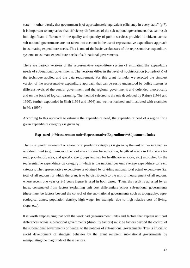
42

state - in other words, that government is of approximately equivalent efficiency in every state” (p.7).

It is important to emphasize that efficiency differences of the sub-national governments that can result

into significant differences in the quality and quantity of public services provided to citizens across

sub-national governments are not taken into account in the use of representative expenditure approach

in estimating expenditure needs. This is one of the basic weaknesses of the representative expenditure

systems to estimate expenditure needs of sub-national governments.

There are various versions of the representative expenditure system of estimating the expenditure

needs of sub-national governments. The versions differ in the level of sophistication (complexity) of

the technique applied and the data requirement. For this grant formula, we selected the simplest

version of the representative expenditure approach that can be easily understood by policy makers at

different levels of the central government and the regional governments and defended theoretically

and on the basis of logical reasoning. The method selected is the one developed by Rafuse (1986 and

1990), further expounded in Shah (1994 and 1996) and well-articulated and illustrated with examples

in Ma (1997).

According to this approach to estimate the expenditure need, the expenditure need of a region for a

given expenditure category i is given by

Exp_need_i=Measurement unit*Representative Expenditure*Adjustment Index

That is, expenditure need of a region for expenditure category i is given by the unit of measurement or

workload used (e.g., number of school age children for education, length of roads in kilometers for

road, population, area, and specific age groups and sex for healthcare services, etc.) multiplied by the

representative expenditure on category i, which is the national per unit average expenditure for each

category. The representative expenditure is obtained by dividing national total actual expenditure (i.e.

total of all regions for which the grant is to be distributed) to the unit of measurement of all regions,

where recent one year or 3-5 years figure is used in both cases. Then, the result is adjusted by an

index constructed from factors explaining unit cost differentials across sub-national governments

(these must be factors beyond the control of the sub-national governments such as topography, agro-

ecological zones, population density, high wage, for example, due to high relative cost of living,

slope, etc.).

It is worth emphasizing that both the workload (measurement units) and factors that explain unit cost

differences across sub-national governments (disability factors) must be factors beyond the control of

the sub-national governments or neutral to the policies of sub-national governments. This is crucial to

avoid development of strategic behavior by the grant recipient sub-national governments by

manipulating the magnitude of these factors.

43

Usually the units of measurements are not as such source of controversy. The same applies to the

representative/average expenditure since it is a well-developed system with solid theoretical

foundation and empirical evidences from various federal nations and more importantly the

representative revenue system-representative expenditure system is selected and adopted by House of

Federations of the Federal Democratic Republic of Ethiopia. The only problematic and controversial

area is the identification of factors explaining unit cost differentials across regions (disability factors)

and their measurement or estimation. That is, it is important that these factors are identified first and

then their importance be determined to construct an index for each expenditure category and each

regional state.

Adjustment_Index_Exp_need_i=ΣwiXi where Σwi=1.

Where Xis are the factors that explain the per unit cost differential for expenditure category i across

sub-national governments while wi is the weight (importance) attached to factor i in explaining unit

cost differentials across sub-national governments. It is obvious that more than all the issues

mentioned in the representative expenditure system the determination of these weights is the most

problematic and controversial due to reasons explained earlier.

The literature identifies two approaches to determine these weights. The first approach is regression

using time series or panel data which is a preferred approach since it is objective if appropriate data

are available and if the estimation functions are properly specified. The second approach is subjective

judgment by the experts (designers) which will finally be settled through political process –

negotiations among the sub-national governments. For the current federal general-purpose grant

formula, we employ the regression approach to determine the weights in order to reduce subjectivity

that is crucial to build consensus and trust on the process of the grant distribution.

From the aforementioned discussions, we understand that the representative expenditure approach to

the estimation of expenditure needs of sub-national governments involves the following steps:

Step 1: Divide the expenditures of sub-national governments into several categories that

constitute the largest proportion of the total expenditure if not all (say 80-90 percent) of their

total expenditure. We adopted the categories used in the development of the existing FGPG formula

which disaggregated the expenditures into nine categories that, on average, capture about 95 percent

of the total expenditures of the regions except the expenditure category of environmental protection

for which data on main variables (both workload variable and the adjustment factors) could not be

found. These are:

44

i. General Service and administration (Organ of the state, Justice and security, and general

service);

ii. Primary and secondary education (including TVET);

iii. Public health;

iv. Agriculture and Rural development

v. Drinking water development

vi. Rural road construction and maintenance

vii. Urban development; and

viii. Micro and small-scale enterprise (MSE) development

As can be seen from Table 25 below, these eight expenditure categories constitute, on average, more

than 93 percent of the total expenditures of the regional States. The share ranges from the smallest of

about 80 percent for Harari and more than 98 percent for the Somalie regional State.

Step 2: Identify the measurement Unit for each of the expenditure categories – that is, address

the question “what is the most important variable that determines the expenditure of regional

States in category i?”.That is, what are the main drivers of expenditures in each of the major

expenditure functions assigned to sub-national governments (for example, for general administration

it may be population, for elementary education the number of students, or for roads kilometers of

roads to be paved or maintained etc.). Theoretical works on the subject and experiences from many

countries show that for most of the expenditure functions (expenditure categories) assigned to the sub-

national governments, the population size of the sub-national governments is the most appropriate

measurement unit. For education, for example, the size of school age children for the different level of

schooling is the proper variable while for healthcare service either the entire population or special age

categories such as children and elderly are taken as measurement unit. In some cases, it is tempting to

use more than one measurement unit. The challenge with this is the determination of the weights to be

attached to the measurement units selected. For the purpose of the current grant formula, the

measurement units selected for each expenditure category are discussed in some detail in sub-section

4.2 below.

Step 3: Identify determinants of the costs of providing a given level of service other than the

prices of the inputs used by the subnational governments and hence explain unit cost

differentials across the sub-national governments (these are also known as the “disability”

factors). If there are several such factors, a weighted average of the determinants is constructed as a

composite disability index. These factors must be factors beyond the control of the sub-national

governments or they must be policy neutral. However, there is no guarantee that the adjustment

factors will be of the expected sign. When such a problem exists, we rely on the coefficients of the

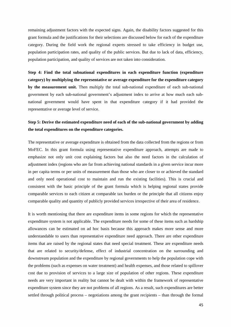
45

remaining adjustment factors with the expected signs. Again, the disability factors suggested for this

grant formula and the justifications for their selections are discussed below for each of the expenditure

category. During the field work the regional experts stressed to take efficiency in budget use,

population participation rates, and quality of the public services. But due to lack of data, efficiency,

population participation, and quality of services are not taken into consideration.

Step 4: Find the total subnational expenditures in each expenditure function (expenditure

category) by multiplying the representative or average expenditure for the expenditure category

by the measurement unit. Then multiply the total sub-national expenditure of each sub-national

government by each sub-national government’s adjustment index to arrive at how much each sub-

national government would have spent in that expenditure category if it had provided the

representative or average level of service.

Step 5: Derive the estimated expenditure need of each of the sub-national government by adding

the total expenditures on the expenditure categories.

The representative or average expenditure is obtained from the data collected from the regions or from

MoFEC. In this grant formula using representative expenditure approach, attempts are made to

emphasize not only unit cost explaining factors but also the need factors in the calculation of

adjustment index (regions who are far from achieving national standards in a given service incur more

in per capita terms or per units of measurement than those who are closer to or achieved the standard

and only need operational cost to maintain and run the existing facilities). This is crucial and

consistent with the basic principle of the grant formula which is helping regional states provide

comparable services to each citizen at comparable tax burden or the principle that all citizens enjoy

comparable quality and quantity of publicly provided services irrespective of their area of residence.

It is worth mentioning that there are expenditure items in some regions for which the representative

expenditure system is not applicable. The expenditure needs for some of these items such as hardship

allowances can be estimated on ad hoc basis because this approach makes more sense and more

understandable to users than representative expenditure need approach. There are other expenditure

items that are raised by the regional states that need special treatment. These are expenditure needs

that are related to security/defense, effect of industrial concentration on the surrounding and

downstream population and the expenditure by regional governments to help the population cope with

the problems (such as expenses on water treatment) and health expenses, and those related to spillover

cost due to provision of services to a large size of population of other regions. These expenditure

needs are very important in reality but cannot be dealt with within the framework of representative

expenditure system since they are not problems of all regions. As a result, such expenditures are better

settled through political process – negotiations among the grant recipients – than through the formal

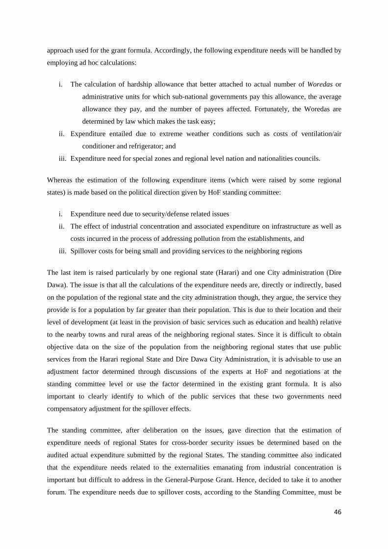
46

approach used for the grant formula. Accordingly, the following expenditure needs will be handled by

employing ad hoc calculations:

i. The calculation of hardship allowance that better attached to actual number of Woredas or

administrative units for which sub-national governments pay this allowance, the average

allowance they pay, and the number of payees affected. Fortunately, the Woredas are

determined by law which makes the task easy;

ii. Expenditure entailed due to extreme weather conditions such as costs of ventilation/air

conditioner and refrigerator; and

iii. Expenditure need for special zones and regional level nation and nationalities councils.

Whereas the estimation of the following expenditure items (which were raised by some regional

states) is made based on the political direction given by HoF standing committee:

i. Expenditure need due to security/defense related issues

ii. The effect of industrial concentration and associated expenditure on infrastructure as well as

costs incurred in the process of addressing pollution from the establishments, and

iii. Spillover costs for being small and providing services to the neighboring regions

The last item is raised particularly by one regional state (Harari) and one City administration (Dire

Dawa). The issue is that all the calculations of the expenditure needs are, directly or indirectly, based

on the population of the regional state and the city administration though, they argue, the service they

provide is for a population by far greater than their population. This is due to their location and their

level of development (at least in the provision of basic services such as education and health) relative

to the nearby towns and rural areas of the neighboring regional states. Since it is difficult to obtain

objective data on the size of the population from the neighboring regional states that use public

services from the Harari regional State and Dire Dawa City Administration, it is advisable to use an

adjustment factor determined through discussions of the experts at HoF and negotiations at the

standing committee level or use the factor determined in the existing grant formula. It is also

important to clearly identify to which of the public services that these two governments need

compensatory adjustment for the spillover effects.

The standing committee, after deliberation on the issues, gave direction that the estimation of

expenditure needs of regional States for cross-border security issues be determined based on the

audited actual expenditure submitted by the regional States. The standing committee also indicated

that the expenditure needs related to the externalities emanating from industrial concentration is

important but difficult to address in the General-Purpose Grant. Hence, decided to take it to another

forum. The expenditure needs due to spillover costs, according to the Standing Committee, must be

47

addressed since it has huge implications for the government of the regional State of Harari and the

Dire Dewa City Administrations in their effort to deliver basic services to their populations.

Accordingly, it was decided that the regional State of Harari and the Dire Dawa City Administration

get an additional 40 percent of their total estimated expenditure needs for healthcare services and

education.

4.2. Actual Expenditures of the Regional States and their Compositions

To understand the trend and the sectoral distributions of the expenditures of the regional States, the

average expenditures of the regional States for the most recent three years (2005-2007) data are used.

Table 24 shows the total actual expenditures of the regional States for the period 2005-2007 EC, the

total average expenditures, and the share of the regional states in the sum total of the expenditures of

the grant recipient regional States and one City Administration.

Table 24: Total actual expenditures of the regional states for the period 2005-2007 EC

Regions Total All Sectors Share of Regions in the total Expenditure

Tigray 7,105,117,623.81 8.54

Afar 2,617,965,323.71 3.15

Amhara 19,348,810,302.72 23.25

Oromia 26,594,064,361.26 31.95

Somale 6,235,495,489.33 7.49

BG 1,640,966,462.04 1.97

S.N.N.P.R 17,052,484,846.20 20.49

Gambella 1,187,838,062.06 1.43

Harari 689,478,816.92 0.83

Diredawa 755,452,196.10 0.91

All Regions 83,227,673,484.15 100

Table 25 presents the actual expenditures of regional States on the eight selected expenditure

categories and the share of the sum total of the expenditures on eight selected expenditure categories

in the total actual average expenditures of the regional States over the three years 2005-2007 EC.

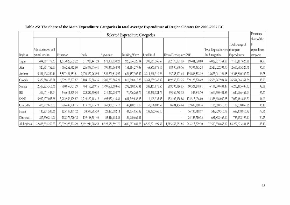
48

Table 25: The Share of the Main Expenditure Categories in total average Expenditure of Regional States for 2005-2007 EC

Administration and general services Education Health Agriculture Drinking Water Rural Road Urban DevelopmenSME

Total Expenditure on the 8 categories

Tigray 1,494,607,777.33 1,673,828,502.22 571,929,441.28 671,300,050.23 920,074,325.34 398,861,566.67 202,775,081.03 89,481,020.80 6,022,857,764.89 7,105,117,623.81 84.77Afar 820,951,752.63 366,262,912.80 226,899,376.41 790,343,664.94 151,114,277.38 68,865,675.13 88,990,540.16 9,594,395.28 2,523,022,594.73 2,617,965,323.71 96.37Amhara 5,381,438,230.46 5,517,421,853.81 2,070,222,962.93 1,526,220,818.97 1,624,457,302.37 2,211,668,310.26 95,763,123.65 195,868,592.19 18,623,061,194.65 19,348,810,302.72 96.25Oromia 5,327,388,335.71 6,879,275,897.87 3,104,157,504.36 2,288,757,585.21 1,816,868,612.23 5,261,839,348.82 469,535,372.25 379,125,328.49 25,526,947,984.94 26,594,064,361.26 95.99Somale 2,519,225,316.36 780,859,757.29 464,155,299.16 1,499,609,688.66 292,310,935.81 248,461,871.63 269,393,316.95 60,524,248.61 6,134,540,434.47 6,235,495,489.33 98.38BG 519,071,443.94 346,614,329.04 223,252,350.54 210,222,250.77 70,776,265.76 134,338,124.76 99,569,788.33 545,848.70 1,604,390,401.85 1,640,966,462.04 97.77SNNP 5,987,677,035.88 3,912,956,129.87 1,719,482,103.12 1,693,932,416.81 691,749,838.95 6,195,333.33 152,102,138.88 174,513,036.00 14,338,608,032.85 17,052,484,846.20 84.09Gambella 475,972,613.63 226,482,798.15 113,778,773.79 167,961,375.12 49,410,512.19 52,098,802.67 8,494,454.44 12,689,180.74 1,106,888,510.73 1,187,838,062.06 93.19Harari 145,231,533.36 123,149,471.12 58,597,895.59 23,487,082.14 44,334,950.32 138,392,466.10 - 16,735,918.17 549,929,316.79 689,478,816.92 79.76Diredawa 217,330,210.99 212,376,720.12 139,468,501.40 53,516,658.86 34,990,661.41 - - 24,135,710.33 681,818,463.10 755,452,196.10 90.25All Regions 22,888,894,250.29 20,039,228,372.29 8,691,944,208.59 8,925,351,591.70 5,696,087,681.78 8,520,721,499.37 1,785,457,781.85 963,213,279.30 77,510,898,665.17 83,227,673,484.15 93.13

Regions

Selected Expenditure Categories

Total average of three years Expenditures

Percentage share of the 8 expenditure categories

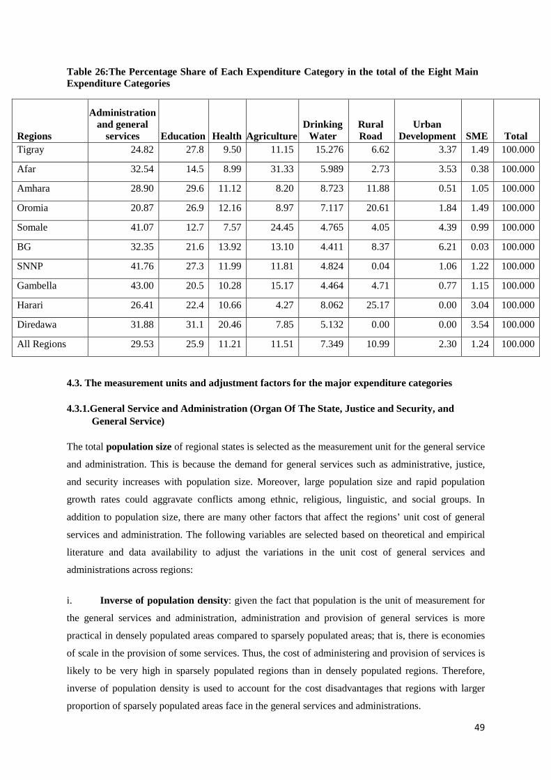
49

Table 26:The Percentage Share of Each Expenditure Category in the total of the Eight Main Expenditure Categories

4.3. The measurement units and adjustment factors for the major expenditure categories

4.3.1.General Service and Administration (Organ Of The State, Justice and Security, and General Service)

The total population size of regional states is selected as the measurement unit for the general service

and administration. This is because the demand for general services such as administrative, justice,

and security increases with population size. Moreover, large population size and rapid population

growth rates could aggravate conflicts among ethnic, religious, linguistic, and social groups. In

addition to population size, there are many other factors that affect the regions’ unit cost of general

services and administration. The following variables are selected based on theoretical and empirical

literature and data availability to adjust the variations in the unit cost of general services and

administrations across regions:

i. Inverse of population density: given the fact that population is the unit of measurement for

the general services and administration, administration and provision of general services is more

practical in densely populated areas compared to sparsely populated areas; that is, there is economies

of scale in the provision of some services. Thus, the cost of administering and provision of services is

likely to be very high in sparsely populated regions than in densely populated regions. Therefore,

inverse of population density is used to account for the cost disadvantages that regions with larger

proportion of sparsely populated areas face in the general services and administrations.

Regions

Administration and general

services Education Health Agriculture Drinking

Water Rural Road

Urban Development SME Total

Tigray 24.82 27.8 9.50 11.15 15.276 6.62 3.37 1.49 100.000

Afar 32.54 14.5 8.99 31.33 5.989 2.73 3.53 0.38 100.000

Amhara 28.90 29.6 11.12 8.20 8.723 11.88 0.51 1.05 100.000

Oromia 20.87 26.9 12.16 8.97 7.117 20.61 1.84 1.49 100.000

Somale 41.07 12.7 7.57 24.45 4.765 4.05 4.39 0.99 100.000

BG 32.35 21.6 13.92 13.10 4.411 8.37 6.21 0.03 100.000

SNNP 41.76 27.3 11.99 11.81 4.824 0.04 1.06 1.22 100.000

Gambella 43.00 20.5 10.28 15.17 4.464 4.71 0.77 1.15 100.000

Harari 26.41 22.4 10.66 4.27 8.062 25.17 0.00 3.04 100.000

Diredawa 31.88 31.1 20.46 7.85 5.132 0.00 0.00 3.54 100.000

All Regions 29.53 25.9 11.21 11.51 7.349 10.99 2.30 1.24 100.000

50

ii. Urbanization rate: Rate of urbanization – defined for the purpose of this grant formula as the

rate of increasing urban population - included in the adjustment factor for general services and

administration to account for the problems and challenges posed by increasing urban population.

Rapid urbanization rate is often associated with high rural to urban migration and a decline in

traditional social values and community spirit in developing countries which could consequently lead

to higher crime rates that in turn increases the demand for more resources to build institutions such as

police and other law enforcement institutions to counteract the undesirable consequences of rapid

urbanization rates across regions.

iii. Size of pastoral population: since pastoralists move from place to place in different seasons

in search of water and grazing land for their animals, it would be costly to administer and to provide

general services in pastoralist areas than in sedentary areas. Pastoralists are also more vulnerable to

drought and they have limited mitigation mechanisms as they do not store food. Moreover, regional

governments (with the help of federal government) have started implementing villagization programs

through water developments in predominantly pastoralist areas to reduce the frequency of their

movement in search of water and animal food and to transform their life into sedentary agriculture.

This implies that regions with large number of pastoral community incur more cost than regions with

low number of pastoral community and hence the size of pastoral population is used as one of the

adjustment factors for general services and administration expenditure category.

Table 27: Total Estimated Expenditure Needs of Regional States for Basic Administration and

General Services

Region

Three-year Average actual expenditure (2005- 2007EC)

Average population size (2005 to 2007EC)

Representative expenditure

Total Expenditure Need - before adjustment

Adjustment index

Total Expenditure Needs after adjustment

Tigray 1,494,607,777 4,960,333 270 1,341,341,952 1.00 1,341,341,952 Afar 820,951,753 1,678,333 270 453,844,288 1.29 584,834,412 Amhara 5,381,438,230 20,015,333 270 5,412,419,584 1.00 5,412,419,584 Oromia 5,327,388,336 32,818,667 270 8,874,615,808 1.00 8,874,615,808 Somali 2,519,225,316 5,308,000 270 1,435,355,776 1.75 2,517,493,940

BG 519,071,444 976,000 270 263,923,744 1.05 277,076,808

S.N.N.P.R 5,987,677,036 17,838,333 270 4,823,729,152 1.00 4,823,729,152 Gambela 475,972,614 396,000 270 107,083,808 1.00 107,083,808 Harari 145,231,533 226,000 270 61,113,488 1.00 61,113,488 Dire Dawa 217,330,211 427,000 270 115,466,632 1.00 115,466,632 Total 22,888,894,250 84,644,000

22,888,894,232

24,115,175,584

51

Note: even though the inverse of population density was among the adjustment factors, its coefficient was negative and hence its coefficient was not used in the calculation of the adjustment weight.

Accounting for Regions’ Security/Defense Related Expenditures

According to the Federal Constitution, defense and security along the country’s international borders

are the responsibilities of the Federal Government. However, some regions are forced to bear

significant amount of expenditure to ensure the security of their region and thereby the whole nation.

The estimation need for this purpose is not straight forward to apply the representative expenditure

approach. First, the problem applies only to some of the regional states and it has no specific

expenditure line. As a result, the data for this expenditure category cannot be found from Federal

offices, which leads to the second problem. Second, as the data for this expenditure come from grant

recipients it leads to the development of strategic behavior by the regional states, which violates one

of the basic principle underlining representative expenditure system and other grant distribution

approaches.

As discussed above, these issues were brought to the attention of the HoF so that directions are given

on how to handle this expenditure category. Accordingly, the HoF indicated that the problem was

raised in the process of the development of the existing grant formula where decision was made to

include regional governments’ estimated expenditure on cross-border conflict in the block grant

formula based on the audited actual expenditure of the regions.

In the existing grant formula, this expenditure category was captured for all regional governments that

have international borders; that is, except Harari Region and Dire Dawa City Administration. In the

existing grant formula, it is indicated that conflicts in relation to international border are very serious

in Tigray and Somalie followed by Afar, Amhara, BenishangulGumuz and Gambella. It was also

argued that some levels of international border related conflicts exist in Oromia and SNNP. Based on

these arguments it was decided that in addition to the estimated expenditure needs, Tigray, Amhra and

Somali obtain additional 40 percent of average of their three year expenditure on security and justices,

Afar, Oromia, SNNP, BenishangulGumuz and Gambella receive 15 percent. It was decided by the

HoF that the expenditure need of each region be determined by the expenditure data on this specific

item that each region presents. In case regions fail to present reliable data, they get the 15 percent

determined in the previous formula. However, it was not easy to get reliable data on cross-border

related security issues as regions report the total expenditure on justice and security. As noted below,

only the Tigray national regional State submitted detail data on this expenditure item. As a

consequence, the estimated expenditure needs for cross-border security in the previous formula is

maintained. Accordingly, Tigray, Amhra and Somali obtain 40 percent of their three-year average

expenditure on security and justices while Afar, Oromia, SNNP, BG and Gambella 15 percent of their

three-year average expenditure on security and justices.

52

Table 28: Estimated Expenditure Needs for Security/Defense Related Expenditures

It is worth mentioning that Tigray region reported a detailed data on its annual expenditure for border

related conflicts and security issues (which includes training expenses, monthly allowances, weapons

and other field instruments, payments to defecting enemy combatants, etc.) that amounts to

ETB217,948,990.00. This amount is 38 percent of the region’s 3-year average expenditure on justice

and security. No such detail data are available for other regions and hence the share used in the

existing grant formula was applied for all regions.

Expenditure Need for Hardship Allowance and Extreme Weather Condition

Regional states pay hardship allowances for employees who are working in very remote and

extremely hot areas. In many cases, the allowances vary between 30 to 40 percent of their salary. This

hardship allowances are supposed to compensate workers for additional expenditure they would incur

due to the extreme weather condition and remoteness. Moreover, air condition and ventilation are

used in many offices mainly in Gambella, Benshangul-Gumuz, Afar, and Dire Dawa. Therefore, it is

reasonable at least to account for the regions’ expenditure need for hardship allowance and extreme

weather condition.

Hardship allowances are calculated for areas where regional governments pay hardship allowance

based on the number of Woredas identified in the process of developing the existing grant formula.

Regions

Three Year Average actual Expenditure on Justice and security of regions

Estimated share of border conflict related expenditure

Estimated Expenditure Need related to cross border security

Tigray 580,857,008.09 0.40 232,342,803.24 Afar 267,869,904.37 0.15 40,180,485.66 Amhara 1,308,613,038.62 0.40 523,445,215.45 Oromia 2,010,047,098.36 0.15 301,507,064.75 Somale 567,174,649.29 0.40 226,869,859.72 BG 133,916,130.22 0.15 20,087,419.53 S.N.N.P.R 1,365,301,709.16 0.15 204,795,256.37 Gambella 146,679,051.79 0.15 22,001,857.77 Harari 34,383,871.92 0.00 - Diredawa 82,249,940.83 0 - Total 6,497,092,402.65

1,571,229,962.49

53

Table 29: Total Estimated Expenditure Needs for Hardship Allowance

It is worth emphasizing that the estimation of regions’ costs for air conditioning, ventilation and

refrigeration is difficult as the prices for different brands and different sizes vary significantly.

Therefore, the estimate is very rough and it may not account fully for their expenditure needs. For air

conditioning and ventilation, the 10 regional bureau offices for air conditioning and 500 offices for

ventilation in the four regions namely Gambella, Benshangul-Gumuz, Afar and Dire Dawa were

accounted. Moreover 20 Refrigerators per Woreda is accounted for Woredas where hardship

allowance is being paid. The annual expenditure need per refrigerator (including the prorated cost of

acquiring a refrigerator plus cost of electricity) is estimated to be Birr 12,000.00 while annual cost of

air conditioner including electricity for regional states is estimated to be Birr 1,400,000.00 (based on

the estimated value in the existing grant formula), 500 offices ventilation cost is estimated at ETB

347,500.00 which again includes the prorated cost of acquiring plus the electricity cost.

Region

Number of woredas

Average allowance rate applied to all regions

Number of woreda with hardship allowance in 2002EC

Annual Salary expenditure (2005-2007 EC Average)

Per woreda annual Salary expenditure (2005-2007 EC Average)

Annual salary estimate for hardship allowance woredas

Annual hardship allowance estimate for hardship woredas, in Birr

Tigray 47 0.35 12 2,602,827,930.67 55,379,317.67 664,551,812.09 232,593,134.23

Afar 30 0.32 17 715,282,964.00 23,842,765.47 405,327,012.93 129,704,644.14

Amhara 138 0.3 6 8,100,136,932.33 58,696,644.44 352,179,866.62 105,653,959.99

Oromia 278 0.28 31

11,981,337,707.67 43,098,337.08 1,336,048,449.42 374,093,565.84

Somali 54 0.31 47 1,772,875,032.00 32,831,019.11 1,543,057,898.22 478,347,948.45

BG 20 0.24 5 720,899,605.00 36,044,980.25 180,224,901.25 43,253,976.30

S.N.N.P.R 145 0.36 10 6,754,484,189.00 46,582,649.58 465,826,495.79 167,697,538.49

Gambella 13 0.32 13 602,984,360.67 46,383,412.36 602,984,360.67 192,954,995.41

Harari 2 0 0 216,237,850.00 108,118,925.00 - -

Dire Dawa 6 0.31 6 324,153,658.00 54,025,609.67 324,153,658.00 100,487,633.98

National 733 0.31 141

33,791,220,229.33 46,099,891.17 6,500,084,655.30 1,824,787,396.82

54

Table 30: Estimated Expenditure Needs for Extreme Weather Condition

Expenditure at region level, Birr Number of Woredas paying hardship allowance

Woredas’ refrigeration cost

Both total region and Woredas’ cost, Birr

Region Ventilation cost

Air conditioner cost Refrigeration Total cost

Tigray 0 12 2,880,000 2,880,000

Afar 347,500.00 1,400,000.00 500,000.00

2,247,500.00

17.00

4,080,000.00

6,327,500.00

Amhara -

6.00

1,440,000.00

1,440,000.00

Oromia -

31.00

7,440,000.00

7,440,000.00

Somali -

47.00

11,280,000.00

11,280,000.00

BG 347,500.00 1,400,000.00 500,000.00

2,247,500.00

5.00

1,200,000.00

3,447,500.00

SNNPR -

10.00

2,400,000.00

2,400,000.00

Gambella 347,500.00 1,400,000.00 500,000.00

2,247,500.00

13.00

3,120,000.00

5,367,500.00

Harari -

-

-

-

Dire Dawa 347,500.00 1,400,000.00 500,000.00

2,247,500.00

-

-

2,247,500.00

Total 42,830,000.00

Expenditure Need for special zones and regional level nation and nationalities councils

The regional states also incur cost for the support of nationalities that is aimed at addressing

ethnic diversities through supporting special zones and/or ethnic minorities. Moreover, two

regions (SNNP and Harari) have council of nationalities at regional level. Therefore, it has been

found reasonable to account (1) for supporting nation and nationalities, and (2) for regional level

HoFs. To estimate the budget need for supporting nations and nationalities, actual and estimated

expenditure need from Gambella, SNNP, Tigray, Amhara and Harai regions are used. The

estimated expenditure need per nationality is Birr 3.5 million per year based on the actual three-

year data by SNNP. Regions’ expenditure need to support nations and nationalities is computed as

Birr 3.5 million times the number of nations and nationalities in the region. To estimate the

expenditure needs for regional HoF, actual expenditure data of SNNP and Harari regions is used.

The estimated budget need for regional HoF is found to be Birr 229,772 per nationality. Then the

expenditure need for regional HoF is computed as the number of nations and nationalities that

exist in the region times Birr 229,772.

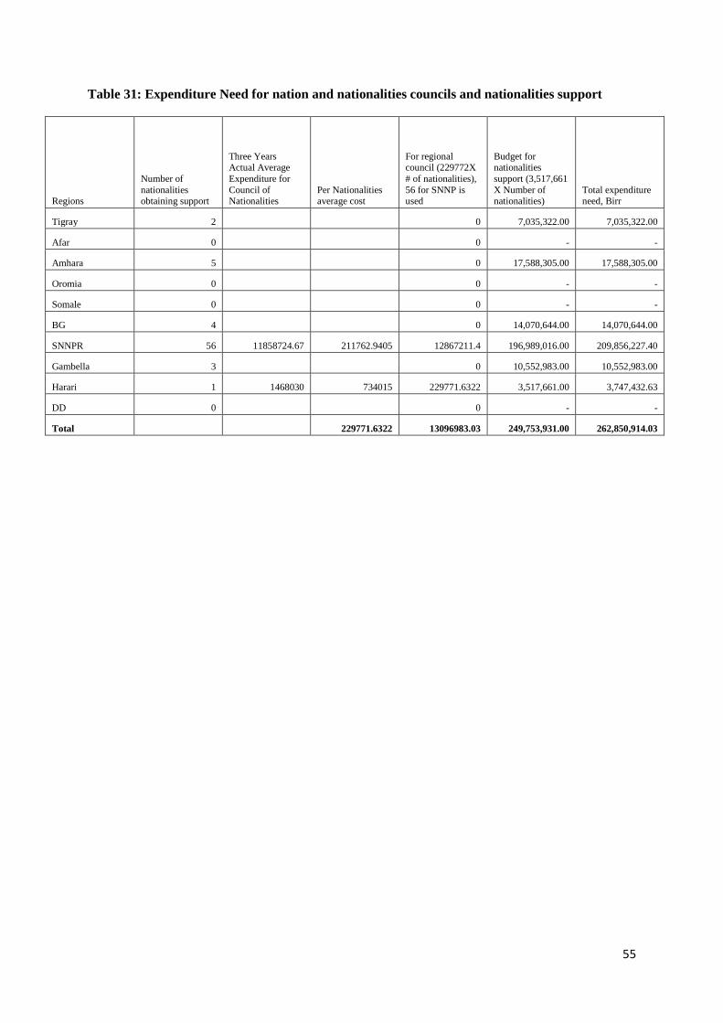
55

Table 31: Expenditure Need for nation and nationalities councils and nationalities support

Regions

Number of nationalities obtaining support

Three Years Actual Average Expenditure for Council of Nationalities

Per Nationalities average cost

For regional council (229772X # of nationalities), 56 for SNNP is used

Budget for nationalities support (3,517,661 X Number of nationalities)

Total expenditure need, Birr

Tigray 2

0 7,035,322.00 7,035,322.00

Afar 0

0 - -

Amhara 5

0 17,588,305.00 17,588,305.00

Oromia 0

0 - -

Somale 0

0 - -

BG 4

0 14,070,644.00 14,070,644.00

SNNPR 56 11858724.67 211762.9405 12867211.4 196,989,016.00 209,856,227.40

Gambella 3

0 10,552,983.00 10,552,983.00

Harari 1 1468030 734015 229771.6322 3,517,661.00 3,747,432.63

DD 0

0 - -

Total

229771.6322 13096983.03 249,753,931.00 262,850,914.03

56

Table32: Total Estimated Expenditure Needs of Regional States for Administration and General Services

Region

Estimated Expenditure Needs for Basic Administration and General Services

Estimated Expenditure Need for cross border security

Estimated Expenditure Need for nation and nationalities councils and nationalities support

Estimated Expenditure Needs for hardship allowance

Estimated Expenditure Needs for Extreme Weather Condition

Total expenditure Need for General Services and Administration

Tigray 1,341,341,952.00 232,342,803.24 7,035,322.00 232,593,134.23 2,880,000.00 1,816,193,211.47 Afar 584,834,412.07 40,180,485.66 - 129,704,644.14 6,327,500.00 761,047,041.86 Amhara 5,412,419,584.00 523,445,215.45 17,588,305.00 105,653,959.99 1,440,000.00 6,060,547,064.43 Oromia 8,874,615,808.00 301,507,064.75 - 374,093,565.84 7,440,000.00 9,557,656,438.59

Somali 2,517,493,939.99 226,869,859.72 - 478,347,948.45

11,280,000.00 3,233,991,748.16 B. Gumuz 277,076,808.01 20,087,419.53 14,070,644.00 43,253,976.30 3,447,500.00 357,936,347.85 SNNPR 4,823,729,152.00 204,795,256.37 209,856,227.40 167,697,538.49 2,400,000.00 5,408,478,174.26 Gambella 107,083,808.00 22,001,857.77 10,552,983.00 192,954,995.41 5,367,500.00 337,961,144.18 Harari 61,113,488.00 - 3,747,432.63 - - 64,860,920.63 Dire Dawa 115,466,632.00 - - 100,487,633.98 2,247,500.00 218,201,765.98

Total

24,115,175,584.08 1,571,229,962.49 262,850,914.03

1,824,787,396.82

42,830,000.00

27,816,873,857.42

57

4.3.2. Primary and secondary education (including TVET)

The expenditure need of regional States for education is computed by disaggregating the total

expenditure into capital expenditure and recurrent expenditure needs. The capital expenditure need

enables to reduce the regional disparity in the access and quality of education and to fulfill each

individual’s constitutional right for equal access to government provided services. The recurrent

expenditure need, on the other hand, is used to maintain those that are already enrolled in the

education system. Since consumers of education services are predominantly specific age groups, we

use school age population (instead of total population) as the units of measurement in the estimation

of the education expenditure needs of regions. Primary school education is from age 7 to 14 (grades 1

to 8) and secondary school education is from ages 15 to 18 (grades 9 to 12). Students leaving at grade

10 can also go to Technical and Vocational Education and Training (TVET).

Capital Expenditure

The unit of measurement for the capital expenditure need is the size of school age population outside

school. Like the general services and administration, to take account of unit cost differences across

regions, the expenditure needs of education are also adjusted by the following disability factors:

i. Inverse of population density: The rationale of using the inverse of population density in the

estimation of the capital and recurrent expenditure needs of regions is similar to the explanation

offered in the general services and administration. In general, the larger the population the higher the

expenditure need for merit goods such as education. Regions with densely populated areas could also

have economies of scale advantage in the supply of education compared to regions with scattered

distribution of population.

ii. Student to class ratio: This adjustment factor enters only in the estimation of the capital

expenditure needs of education. Regions with large number of school age population outside school

require more resources for constructing class rooms to enroll those who are not in school. At the same

time regions with larger student class ratio need to construct more facilities to meet the national

standards with respect to this factor which is claimed to have impact on quality of education.

58

Table 33: Estimated Capital expenditure Need for Primary Education

Table 34: Estimated Capital expenditure Need for Secondary and TVET

region Name

Three Year Average Expenditure (2005 to 2007EC)

School age population 7-17 (2005 to 2007EC)

Representative expenditure

Total Expenditure Need before adjustment

Adjustment index

Total Estimated Expenditure need after adjustment

Tigray 77,789,606.67 1,008,110.33 48 47,904,566.31 0.80 1.00 47,904,566.31

Afar 63,577,906.00 307,379.67 48 14,606,426.63 0.87 1.00 14,606,426.63

Amhara 4,922,383.00 3,889,345.67 48 184,818,477.92 0.89 1.00 184,818,477.92

Oromia 270,066,329.33 7,228,621.67 48 343,498,101.84 1.10 1.10 378,191,410.13

Somali 9,459,348.00 953,415.67 48 45,305,521.14 1.53 1.53 69,408,058.39

BG 47,021,516.67 194,172.00 48 9,226,892.28 1.00 1.00 9,226,892.28

SNNPR 273,625,900.33 3,950,350.67 48 187,717,384.89 1.16 1.16 218,315,318.63

Gambela 27,680,854.00 76,833.00 48 3,651,040.39 1.05 1.05 3,848,196.57

Harari - 40,606.67 48 1,929,595.10 0.84 1.00 1,929,595.10

Dire Dawa 35,448,044.67 82,756.00 48 3,932,496.43 0.76 1.00 3,932,496.43

Total 809,591,888.67 17,731,591.33

842,590,502.94

932,181,438.39

Region

Three years average actual expenditure (2005 to 2007EC)

School age population 15-18 (2005 to 2007EC)

Representative expenditure

Total Expenditure Need before adjustment (=D*E)

Adjustment index

expenditure need after adjustment

Assuming this capital expenditure is spent over 5 years

Tigray 98,249,933 452,760 1,526 690,968,299 1.000 690,968,299 138,193,660

Afar 45,855,297 158,875 1,526 242,462,760 1.040 252,161,270 50,432,254

Amhara 293,388,247 1,774,614 1,526 2,708,284,565 1.000 2,708,284,565 541,656,913

Oromia 958,336,090 3,036,112 1,526 4,633,489,971 1.000 4,633,489,971 926,697,994

Somali 199,473,253 503,786 1,526 768,840,913 1.530 1,176,326,597 235,265,319

Benishangul-Gumuz 21,756,725 85,200 1,526 130,025,426 1.000 130,025,426 26,005,085

SNNPR 304,336,090 1,673,506 1,526 2,553,981,018 1.000 2,553,981,018 510,796,204

Gambela 16,579,166 36,087 1,526 55,073,309 1.410 77,653,366 15,530,673

Harari 396,244 19,181 1,526 29,273,132 1.000 29,273,132 5,854,626

Dire Dawa 396,244 41,448 1,526 63,254,870 1.000 63,254,870 12,650,974

Total 1,938,767,289 7,781,569

11,875,654,263

12,315,418,514 2,463,083,703

59

Recurrent Expenditure

The measurement unit for the recurrent expenditure is the total school age population because

education expenditure is directly linked to school age population and the measure is beyond the

control of the regional governments. Attempts were made to use adjustment factors such as inverse of

population density, proportion of female students and so on. But the result obtained after adjusting has

large difference from the average of the actual expenditure of regions. Therefore, the recurrent

expenditures on both primary and secondary are not adjusted.

Table 35: Recurrent Expenditure for Primary Education

The implication of number of languages used in education in the regions: Some of the regional

states provide education in more than one language which increases their expenditure needs

particularly for the development of textbooks3. These imply that the expenditure on education is an

increasing function of the number of languages used as a medium of instruction in each regional State.

The number of languages used in education was used as an adjustment factor; however, the estimated

result was highly unrealistic. This could be due to the outlier regional State – SNNP – with a number

of languages in which education is claimed to be offered more than 10-fold of the second largest. As a

result, an ad hoc method is adopted to take care of the implication of the number of languages

particularly on expenditure of regions on textbook development used in the previous grant distribution

formula by updating daily payments for experts from ETB 1500 to ETB 2000.

3It is also important to note that regional States who offer education in more than one language incur costs for researches on the use of the language as a medium of instruction. However, this cost is not captured in this grant formula due to lack of reliable data.

Region

Three years average actual expenditure (2005 to 2007EC)

School age Children (2005 - 2007EC)

Representative expenditure

Total Estimated Expenditure Needs of Regional States

Tigray 129,228,021 1,008,110 535 538,883,665 Afar 140,153,037 307,380 535 164,309,278 Amhara 2,712,951,302 3,889,346 535 2,079,043,114 Oromia 3,596,083,302 7,228,622 535 3,864,047,423 Somali 57,621,021 953,416 535 509,646,724 BG 168,471,079 194,172 535 103,794,313 SNNPR 2,145,748,605 3,950,351 535 2,111,653,233 Gambela 91,237,996 76,833 535 41,070,950 Harari 52,685,510 40,607 535 21,706,225 Dire Dawa 13,007,208 82,756 535 44,237,079

Total 9,107,187,082.00 17,731,591.33

9,478,392,003.53

60

Using the ministry of education specification, text book development requires four experts:

- Subject area specialist;

- Pedagogical designer (what activities and illustration);

- Illustration specialist; and

- An Editor

Subject area specialist and Pedagogical designer work together and need up to five full months. That

is, they require 10-person months at a rate of Birr 2000 per day (10*30*2000=600,000). Illustrative

specialists (or artists) require two-person months at a rate ETB 2000 = (1*2*30*2000=120,000),

while an Editor requires one person month (30*2000=60,000). In total, one text book preparation

requires ETB 780,000. This is assumed to serve for five years and hence per year cost to develop a

text book per subject is Birr 156,000.

Table 36: Estimated Expenditure Needs of Regional States for Textbook Development

Region

Number of language used

Number of languages that need text book

Total textbooks Unit cost

Total budget for text book development

Tigray 4 3 75 156,000.00 11,700,000.00 Afar 3 2 50 156,000.00 7,800,000.00 Amhara 5 4 125 156,000.00 19,500,000.00 Oromia 2 1 25 156,000.00 3,900,000.00 Somali 2 1 25 156,000.00 3,900,000.00 BG 6 5 125 156,000.00 19,500,000.00 SNNPR 57 56 1400 156,000.00 218,400,000.00 Gambella 5 4 100 156,000.00 15,600,000.00 Harari 3 2 50 156,000.00 7,800,000.00 Dire Dawa 3 2 50 156,000.00 7,800,000.00

Total

315,900,000.00

Table 37: Recurrent Expenditure for Secondary Education and TVET

region Name

Three-year average Expenditure (2005 to 2007EC)

School age population (age 15-18) (2005 to 2007EC)

Representative expenditure

Total Expenditure need before adjustment

Tigray 1,267,453,822 452,760 721 326,417,942 Afar 68,851,232 158,875 721 114,540,993 Amhara 1,555,289,157 1,774,614 721 1,279,411,335 Oromia 2,025,655,809 3,036,112 721 2,188,890,955 Somali 91,088,094 503,786 721 363,205,474

61

BG 82,860,320 85,200 721 61,425,102 SNNPR 355,218,382 1,673,506 721 1,206,517,330 Gambela 60,897,752 36,087 721 26,016,991 Harari 32,107,600 19,181 721 13,828,819 Dire Dawa 70,714,666 41,448 721 29,882,014

Total 5,610,136,834 7,781,569

5,610,136,956

62

Table 38: Total Estimated Expenditure Needs of Regional States for Education

Regions

Recurrent Expenditure Need Primary Education

Capital Expenditure Need Primary education

Expenditure Need for Textbook Development

Recurrent Secondary and TEVT

Capital Secondary and TEVT

Total Education before Adjustment for spillover

Spillover Rate

Estimated Compensatory Adjustment for Spillover Effect

Total Estimated Expenditure Need for Education

Tigray 538,883,664.90 47,904,566.31 11,700,000.00 326,417,941.93 138,193,659.81 1,063,099,832.94 - - 1,063,099,832.94

Afar 164,309,278.27 14,606,426.63 7,800,000.00 114,540,992.80 50,432,253.98 351,688,951.69 - - 351,688,951.69

Amhara 2,079,043,114.23 184,818,477.92 19,500,000.00 1,279,411,335.07 541,656,913.07 4,104,429,840.29 - - 4,104,429,840.29

Oromia 3,864,047,423.26 378,191,410.13 3,900,000.00 2,188,890,955.33 926,697,994.16 7,361,727,782.88 - - 7,361,727,782.88

Somali 509,646,723.81 69,408,058.39 3,900,000.00 363,205,473.89 235,265,319.39 1,181,425,575.49 - - 1,181,425,575.49

BG 103,794,312.51 9,226,892.28 19,500,000.00 61,425,101.88 26,005,085.30 219,951,391.96 - - 219,951,391.96

SNNPR 2,111,653,233.27 218,315,318.63 218,400,000.00 1,206,517,330.36 510,796,203.55 4,265,682,085.81 - - 4,265,682,085.81

Gambela 41,070,949.53 3,848,196.57 15,600,000.00 26,016,991.22 15,530,673.13 102,066,810.45 - - 102,066,810.45

Harari 21,706,224.64 1,929,595.10 7,800,000.00 13,828,818.71 5,854,626.30 51,119,264.75 0.30 15,335,779.42 66,455,044.17 Dire Dawa 44,237,079.11 3,932,496.43 7,800,000.00 29,882,014.35 12,650,974.09 98,502,563.99 0.30 29,550,769.20 128,053,333.18

Total 9,478,392,003.53 932,181,438.39 315,900,000.00 5,610,136,955.53 2,463,083,702.79 18,799,694,100.24

44,886,548.62 18,844,580,648.86

63

4.3.3. Public Health The estimation of the regions’ health expenditure need is implemented disaggregating the total into

capital expenditure and recurrent expenditure needs like the approach we followed for education

expenditure needs.

Capital Expenditure

The capital expenditure components are estimated based on the principle of reducing the access gap

and inequality in health services and to fulfill each individual’s right of equal access to government

provided services. The unit of measurement in the estimation of the capital expenditure is the size of

population without access to health services at reasonable distance (depending on the national

standard). The capital expenditure needs for health services are adjusted by the disability factors. The

rationale for choosing these disability factors is presented as follows:

i. Inverse of population density: this adjustment factor is used to account for the difficulties

of providing health services in scattered population.

ii. Population to health facility ratio: larger population to health facility ratio implies larger

capital expenditure need to improve access to health service coverage.

iii. Number of health professionals per population: this adjustment factor is to take health

service quality into consideration. In regions where the number of health professionals per thousand

of population is low, larger resources are needed to improve the health service quality.

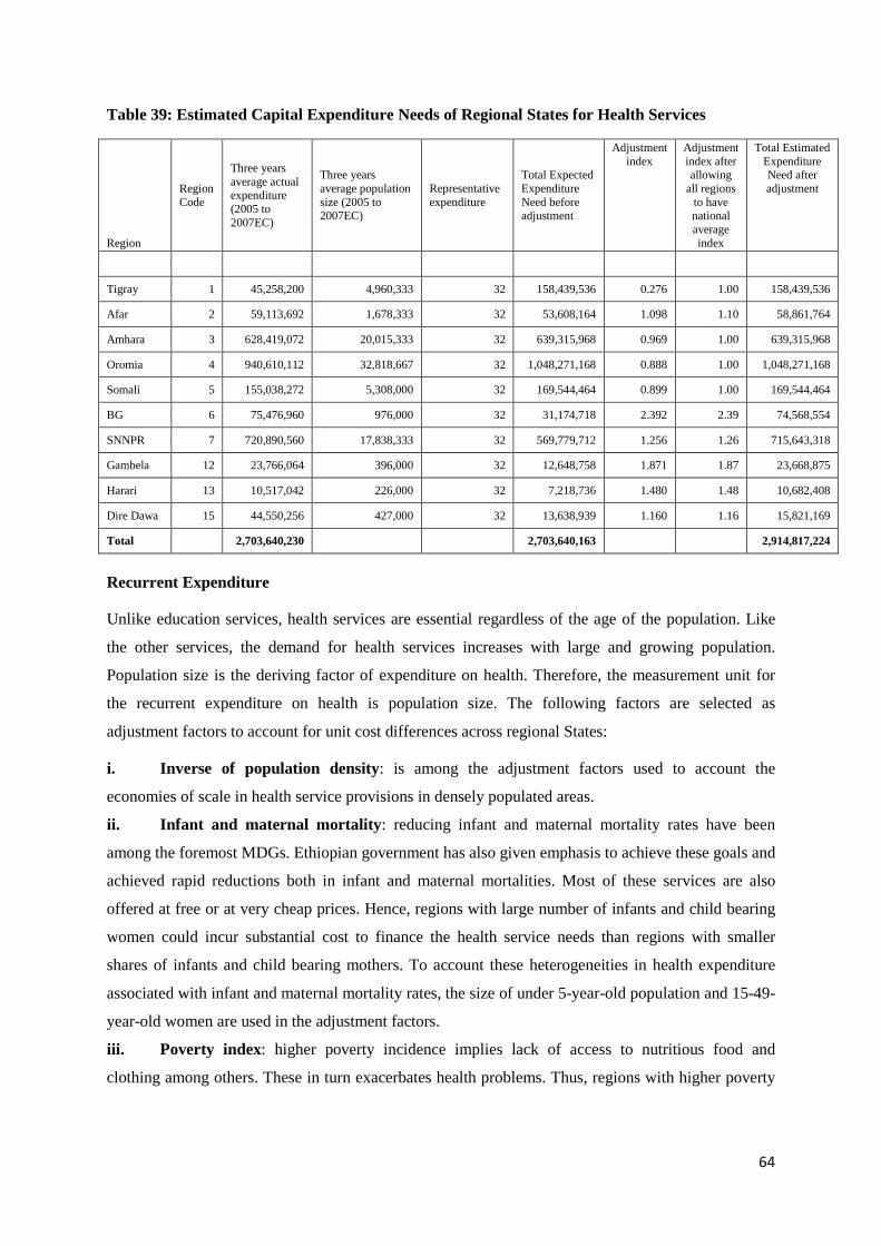
64

Table 39: Estimated Capital Expenditure Needs of Regional States for Health Services

Recurrent Expenditure

Unlike education services, health services are essential regardless of the age of the population. Like

the other services, the demand for health services increases with large and growing population.

Population size is the deriving factor of expenditure on health. Therefore, the measurement unit for

the recurrent expenditure on health is population size. The following factors are selected as

adjustment factors to account for unit cost differences across regional States:

i. Inverse of population density: is among the adjustment factors used to account the

economies of scale in health service provisions in densely populated areas.

ii. Infant and maternal mortality: reducing infant and maternal mortality rates have been

among the foremost MDGs. Ethiopian government has also given emphasis to achieve these goals and

achieved rapid reductions both in infant and maternal mortalities. Most of these services are also

offered at free or at very cheap prices. Hence, regions with large number of infants and child bearing

women could incur substantial cost to finance the health service needs than regions with smaller

shares of infants and child bearing mothers. To account these heterogeneities in health expenditure

associated with infant and maternal mortality rates, the size of under 5-year-old population and 15-49-

year-old women are used in the adjustment factors.

iii. Poverty index: higher poverty incidence implies lack of access to nutritious food and

clothing among others. These in turn exacerbates health problems. Thus, regions with higher poverty

Region

Region Code

Three years average actual expenditure (2005 to 2007EC)

Three years average population size (2005 to 2007EC)

Representative expenditure

Total Expected Expenditure Need before adjustment

Adjustment index

Adjustment index after allowing

all regions to have national average index

Total Estimated Expenditure Need after adjustment

Tigray 1 45,258,200 4,960,333 32 158,439,536 0.276 1.00 158,439,536

Afar 2 59,113,692 1,678,333 32 53,608,164 1.098 1.10 58,861,764

Amhara 3 628,419,072 20,015,333 32 639,315,968 0.969 1.00 639,315,968

Oromia 4 940,610,112 32,818,667 32 1,048,271,168 0.888 1.00 1,048,271,168

Somali 5 155,038,272 5,308,000 32 169,544,464 0.899 1.00 169,544,464

BG 6 75,476,960 976,000 32 31,174,718 2.392 2.39 74,568,554

SNNPR 7 720,890,560 17,838,333 32 569,779,712 1.256 1.26 715,643,318

Gambela 12 23,766,064 396,000 32 12,648,758 1.871 1.87 23,668,875

Harari 13 10,517,042 226,000 32 7,218,736 1.480 1.48 10,682,408

Dire Dawa 15 44,550,256 427,000 32 13,638,939 1.160 1.16 15,821,169

Total 2,703,640,230

2,703,640,163

2,914,817,224

65

incidence could face larger demand for health services and nutrient supplements to protect children

from malnutrition.

Table 40: Estimated Recurrent Expenditure Needs of Regional States for Health Services

Region

Three years average actual expenditure (2005 to 2007EC)

Three years average population size (2005 to 2007EC)

Representative expenditure

Total Expected Expenditure Need before adjustment

Adjustment index

Adjustment index after all regions

are assigned an index of at

least 1

Total Estimated

Expenditure Need after adjustment

Tigray 526,671,232 4,960,333 71 350,928,416 1.50 1.499 526,171,890

Afar 167,785,680 1,678,333 71 118,736,952 1.41 1.410 167,363,771

Amhara 1,441,803,904 20,015,333 71 1,416,023,680 1.02 1.018 1,441,512,106

Oromia 2,163,547,392 32,818,667 71 2,321,820,160 0.93 1.000 2,321,820,160

Somali 309,117,024 5,308,000 71 375,524,768 0.82 1.000 375,524,768

BG 147,775,392 976,000 71 69,049,016 2.13 2.132 147,245,922

SNNPR 998,591,552 17,838,333 71 1,262,007,552 0.79 1.000 1,262,007,552

Gambela 90,012,712 396,000 71 28,015,788 3.20 3.200 89,656,321

Harari 48,080,852 226,000 71 15,988,809 1.99 1.988 31,785,832 Dire Dawa 94,918,248 427,000 71 30,208,944 3.50 3.501 105,748,614

Total 5,988,303,988

5,988,304,085

6,468,836,936

66

Table 41: Total Estimated Expenditure Needs of Regional States for Health Services

4.3.4: Agriculture and Rural development

In GTP II, it is clearly indicated that the agricultural sector would continue to be the main source of

economic growth. In turn, within agriculture, the bulk of the growth is expected to originate from

smallholder farmers’ agriculture. Regional States provide various services to both smallholder farmers

and pastoralists to increase production and productivity and thereby meet the goals of national food

security and sustainable growth. The expenditure on agriculture and rural development is mainly for

crop and livestock production.

For the agriculture and rural development, the unit of measurement selected is the region’s rural

population. The main actors in agriculture and rural development in the country are smallholder

farmers. Training, plot visits, on farm demonstrations, and related costs for agriculture and rural

development mainly depend up on the rural population. Hence, the number of rural population is the

driving force of expenditure needs of regional governments for agriculture and rural development.

Though the size of rural population is the driving force of the expenditure needs of regional States for

agriculture and rural development, there are other factors that explain unit cost differences across

regions. The contributors for variations in expenditure need on agriculture and rural development

mainly include: inverse of density of rural population, size of arable land, tropical livestock unit and

Regions

Total Estimated Expenditure Need for Recurrent Expenditure

Total Estimated Expenditure Need for Capital

Total Estimated Expenditure Need for Health Services before Adjustment for Spillover Effects

Rate of Spillover Effect

Estimated Compensatory Adjustment for Spillover Effect

Total Estimated Expenditure Need for Health Services

Tigray 526,171,890.03 158,439,536.00 684,611,426.03 - - 684,611,426.03

Afar 167,363,770.90 58,861,764.07 226,225,534.97 - - 226,225,534.97

Amhara 1,441,512,106.24 639,315,968.00 2,080,828,074.24 - - 2,080,828,074.24

Oromia 2,321,820,160.00

1,048,271,168.00 3,370,091,328.00 - - 3,370,091,328.00

Somali 375,524,768.00 169,544,464.00 545,069,232.00 - - 545,069,232.00

BG 147,245,921.84 74,568,553.77 221,814,475.60 - - 221,814,475.60

SNNPR 1,262,007,552.00 715,643,318.27 1,977,650,870.27 - - 1,977,650,870.27

Gambela 89,656,320.87 23,668,874.57 113,325,195.44 -

113,325,195.44

Harari 31,785,832.24 10,682,408.25 42,468,240.49 0.30 12,740,472.15 55,208,712.63

Dire Dawa 105,748,613.72 15,821,169.24 121,569,782.96 0.30 36,470,934.89 158,040,717.85

Total 6,468,836,935.83

2,914,817,224.17 9,383,654,160.00

49,211,407.04 9,432,865,567.04

67

pastoral population. Variation in these factors has an implication on expenditure needs for agriculture

and rural development. Hence, in the expenditure need estimation adjustments are made to take into

account such variations across regions.

i. Inverse of density of rural population: Population dispersion increases the cost of offering

trainings, plot visits and demonstration activities of the development agents. Thus, inverse of

population density is used to adjust for the impact of population dispersion on the cost of delivering

services to crop producing smallholder rural households.

ii. Size of arable land: As the size of the arable land of the region increases there is a need for

more FTC, DAs and more supervision and follow up costs. The development agents are required to

visit the plots of farmers especially the trial plots planted by the model farmers. Thus, larger arable

size could increase the cost of development agent visits. Moreover, larger size in arable land might

require huge resources to protect production loss during some epidemics such as pests and rainfall

during harvest seasons. Regional governments have responsibility to help farmers to overcome such

type of disasters.

iii. Size of pastoral population- pastoralists move from place to place in search of grazing land

and water for their cattle. As a result, supplying animal health services to pastoralist population is

extremely high than in settled agriculture areas. Thus, to ensure access to animal health services for

the pastoralist population, the regional governments should either built veterinaries in all of the

potential destinations of the pastoralists or the regional governments should design veterinary services

which moves from place to place by following the pastoralist communities. Consequently, the regions

with more pastoralists need more expenditure for livestock development than the other regions and

vice versa.

iv. Tropical Livestock Unit (TLU):This a composite measure of the total population of

livestock. The livestock population is used as one of the adjustment factors since regional

governments incur significant expenditure in vaccination during epidemics, preventing and

controlling animal disease outbreaks, and also providing water and fodder especially during drought.

The total cost for these services is, therefore, directly proportional with the livestock population.

68

Table 42: Total Estimated Expenditure Needs of Regional States for Agriculture Development

4.3.5. Provision of Drinking Water

Provision of Drinking Water is an important responsibility for regional States. According to GTP II, at

the end of the plan period the urban potable water supply coverage will reach 100 percent while that

of the rural areas will reach 98 percent. Access to water supply is defined as when people in urban

areas get 30 liters of water within 500 meter and people in rural areas get 15 liters of water within 1.5-

kilometer distance. The 2015 assessment report by JMP indicates that Ethiopia has met the target of

57 percent of the population using safe drinking water and attained the target by halving the number

of people without access to safe water since 1990.

Safe drinking water is financed through government channels and using government implementation

modalities to localized interventions using innovative approaches and direct project financing

mechanisms.

The Unit of measurement to estimate the regions’ expenditure needs for provision of drinking water is

total population. The rationale for this choice is straightforward as larger population implies larger

expenditure to avail water. However, as in the case of other expenditure needs, in addition to

measurement units, there are disability factors that explain unit cost differentials across regional

States in providing drinking water to their respective populations. Some of these disability factors are:

Region

Three-year average Rural Population

Three Year average actual Expenditure

Representative Expenditure

Total Expenditure Need before adjustment

Average of the estimated Weights of Adjustment factors

Total Estimated Expenditure Need after adjustment

Tigray 3,759,666.67 621,307,675.87 92.56 347,994,746.67 1.40 487,988,419.53

Afar 1,388,666.67 748,166,866.19 92.56 128,534,986.67 4.52 580,706,916.48

Amhara

16,887,000.00

1,181,650,303.81 92.56

1,563,060,720.00 1.00 1,563,060,720.00

Oromia

28,164,000.00

1,712,856,999.74 92.56

2,606,859,840.00 1.00 2,606,859,840.00

Somali 4,545,333.33 467,676,828.19 92.56 420,716,053.33 2.61 1,097,950,628.40

BSG 786,666.67 181,709,509.81 92.56 72,813,866.67 2.11 153,611,887.00

SNNPR

15,132,333.33

1,455,439,274.53 92.56

1,400,648,773.33 1.00 1,400,648,773.33

Gambela 271,666.67 138,961,260.00 92.56 25,145,466.67 4.74 119,244,409.56

Harari 101,333.33 16,314,626.41 92.56 9,379,413.33 2.63 24,700,313.37

Dire Dawa 159,000.00 65,928,276.67 92.56 14,717,040.00 2.29 33,681,533.70

Total

71,195,666.67

6,590,011,621.22

6,589,870,906.67

8,068,453,441.39

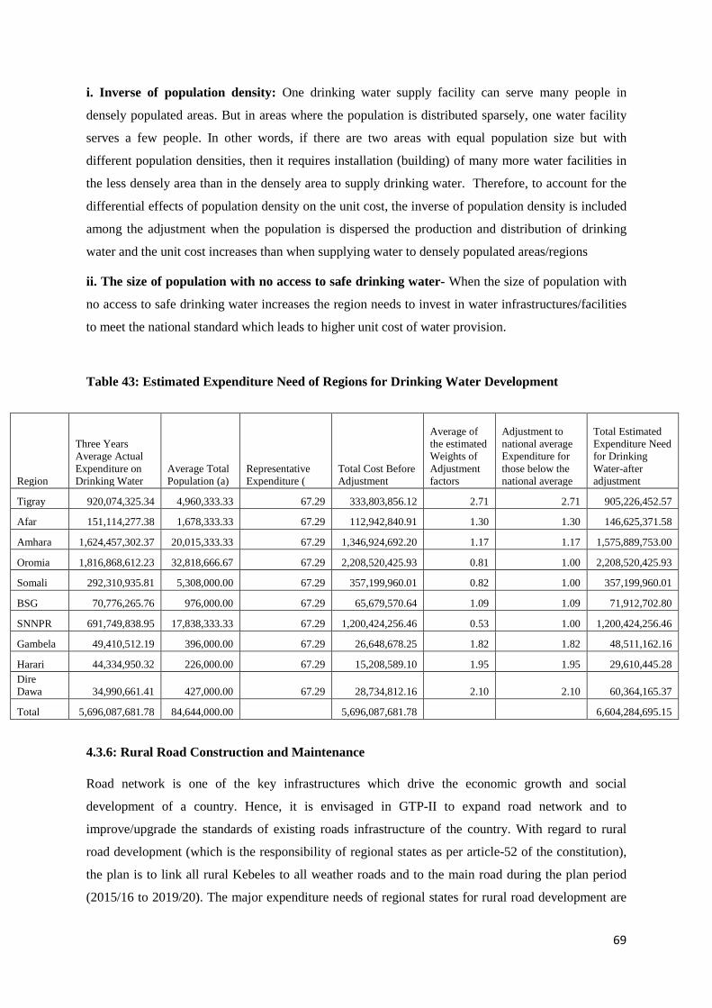
69

i. Inverse of population density: One drinking water supply facility can serve many people in

densely populated areas. But in areas where the population is distributed sparsely, one water facility

serves a few people. In other words, if there are two areas with equal population size but with

different population densities, then it requires installation (building) of many more water facilities in

the less densely area than in the densely area to supply drinking water. Therefore, to account for the

differential effects of population density on the unit cost, the inverse of population density is included

among the adjustment when the population is dispersed the production and distribution of drinking

water and the unit cost increases than when supplying water to densely populated areas/regions

ii. The size of population with no access to safe drinking water- When the size of population with

no access to safe drinking water increases the region needs to invest in water infrastructures/facilities

to meet the national standard which leads to higher unit cost of water provision.

Table 43: Estimated Expenditure Need of Regions for Drinking Water Development

4.3.6: Rural Road Construction and Maintenance

Road network is one of the key infrastructures which drive the economic growth and social

development of a country. Hence, it is envisaged in GTP-II to expand road network and to

improve/upgrade the standards of existing roads infrastructure of the country. With regard to rural

road development (which is the responsibility of regional states as per article-52 of the constitution),

the plan is to link all rural Kebeles to all weather roads and to the main road during the plan period

(2015/16 to 2019/20). The major expenditure needs of regional states for rural road development are

Region

Three Years Average Actual Expenditure on Drinking Water

Average Total Population (a)

Representative Expenditure (

Total Cost Before Adjustment

Average of the estimated Weights of Adjustment factors

Adjustment to national average Expenditure for those below the national average

Total Estimated Expenditure Need for Drinking Water-after adjustment

Tigray 920,074,325.34 4,960,333.33 67.29 333,803,856.12 2.71 2.71 905,226,452.57

Afar 151,114,277.38 1,678,333.33 67.29 112,942,840.91 1.30 1.30 146,625,371.58

Amhara 1,624,457,302.37 20,015,333.33 67.29 1,346,924,692.20 1.17 1.17 1,575,889,753.00

Oromia 1,816,868,612.23 32,818,666.67 67.29 2,208,520,425.93 0.81 1.00 2,208,520,425.93

Somali 292,310,935.81 5,308,000.00 67.29 357,199,960.01 0.82 1.00 357,199,960.01

BSG 70,776,265.76 976,000.00 67.29 65,679,570.64 1.09 1.09 71,912,702.80

SNNPR 691,749,838.95 17,838,333.33 67.29 1,200,424,256.46 0.53 1.00 1,200,424,256.46

Gambela 49,410,512.19 396,000.00 67.29 26,648,678.25 1.82 1.82 48,511,162.16

Harari 44,334,950.32 226,000.00 67.29 15,208,589.10 1.95 1.95 29,610,445.28 Dire Dawa 34,990,661.41 427,000.00 67.29 28,734,812.16 2.10 2.10 60,364,165.37

Total 5,696,087,681.78 84,644,000.00

5,696,087,681.78

6,604,284,695.15

70

costs of constructing new roads (capital expenditures) and costs of maintaining existing roads

(recurrent expenditure).

Capital Expenditure Need

In this case, regions’ average yearly plan for construction of new rural road (which is determined from

five years plan) is used as unit of measurement. The average five years plan is used as proxy for total

length of rural road that need to be constructed to achieve minimum national standard since data is not

available on the prevailing gap in this regard. Here, it is assumed that a region that lag behind in terms

of road accessibility need to construct more KMs of rural road than otherwise so as to ensure

equitable road accessibility.

Representative expenditure (i.e. overall average per kms cost of constructing rural road) is determined

as the ratio of three years average capital expenditure on rural road construction by all regions and the

overall average length of rural road constructed by all regions during the same period.

Disability/Adjustment factors: To account for possible deviation of region specific unit cost from

representative unit cost, an adjustment is made using the following factors:

Weather condition (rain-fall): High mean annual rain implies higher costs for the construction of

rural roads and also needs more selected materials to withstand the effect of rainfall.

Mean slope: Sloppy topography requires building of more supportive structures, bridges and

culverts/drainage/ systems, and also level the land while building new roads, and hence entail more

costs.

Soil type: This factor is included in the adjustment index on the ground that road construction cost

and the cost needed for maintenance depends on the soil cover: removing existing unsuitable soil and

refilling with selected material, and constructing supportive structures as well is necessary with all

additional costs thereof.

In addition to the above variables, inclusion of number of bridges and culverts in the adjustment index

was also suggested by some regions. However, these factors are not considered in estimating rural

road expenditure needs of regions due to absence of data.

71

Table 44: Estimated Capital Expenditure Need of Regional States Rural Roads

Recurrent Expenditure Need

The measurement unit selected for recurrent expenditures is the length of rural road network. This is

so since the major recurrent spending by regional states on rural roads is expenditure on the

maintenance of existing rural roads. The representative expenditure rate (i.e. the overall average

maintenance cost per kms) is determined as the ratio of the sum of three years average expenditure of

all regions to the sum of average yearly road constructed by all regions. Here, had data been available,

using average length of rural road maintained by all regions over the same period would have been

better instead of using average length of road constructed, however, the requisite data is not missing.

Disability/Adjustment Factors: To account for unit cost differential across regions, adjustment is made

using factors such as

i. Traffic rate (proxied by population density): The frequency of maintenance of a road partly

depends on the rate of utilization. Other things remaining the same, roads that are used with high

Region

Three Years Ave. Actual Capital Expenditure on Rural Road Construction

Average yearly road constructed

Average Rural Road Gap in KMs(as proxied by average yearly plan)

Representative Expenditure

Total Cost Before Adjustment

Relative Index of Adjustment

Weighted adjustment index after allowing all regions to have at least the national average

Total Estimated Capital Expenditure Need for Rural Road -after adjustment

Tigray 559,232,762.00 456.60 1,032.80 992,797.58 1,025,361,339 0.96 1.00 1,025,361,339.41

Afar 59,463,002.00

405.40 992,797.58 402,480,138 0.73 1.00 402,480,138.46

Amhara

2,133,368,439.00 1,883.00 4,097.60 992,797.58 4,068,087,359 0.92 1.00 4,068,087,359.01

Oromia

5,487,096,244.33 5,431.60 7,001.00 992,797.58 6,950,575,849 0.87 1.00 6,950,575,849.38

Somali 248,802,044.33

1,323.80 992,797.58 1,314,265,435 0.48 1.00 1,314,265,434.85

BSG 146,840,894.67 73.20 225.20 992,797.58 223,578,015 1.30 1.30 290,651,419.18

SNNPR 361,929,154.00 1,437.00 3,744.40 992,797.58 3,717,431,254 0.34 1.00 3,717,431,254.17

Gambela 63,220,572.33 9.00 85.60 992,797.58 84,983,473 2.59 2.60 220,957,029.14

Harari 143,577,811.67 28.80 27.00 992,797.58 26,805,535 1.47 1.50 40,208,301.94 Dire Dawa 91,040,008.67 42.80 57.20 992,797.58 56,788,022 0.34 1.00 56,788,021.51

Total

9,294,570,933.00 9,362.00

18,000.00

17,870,356,418.93

18,086,806,147.06

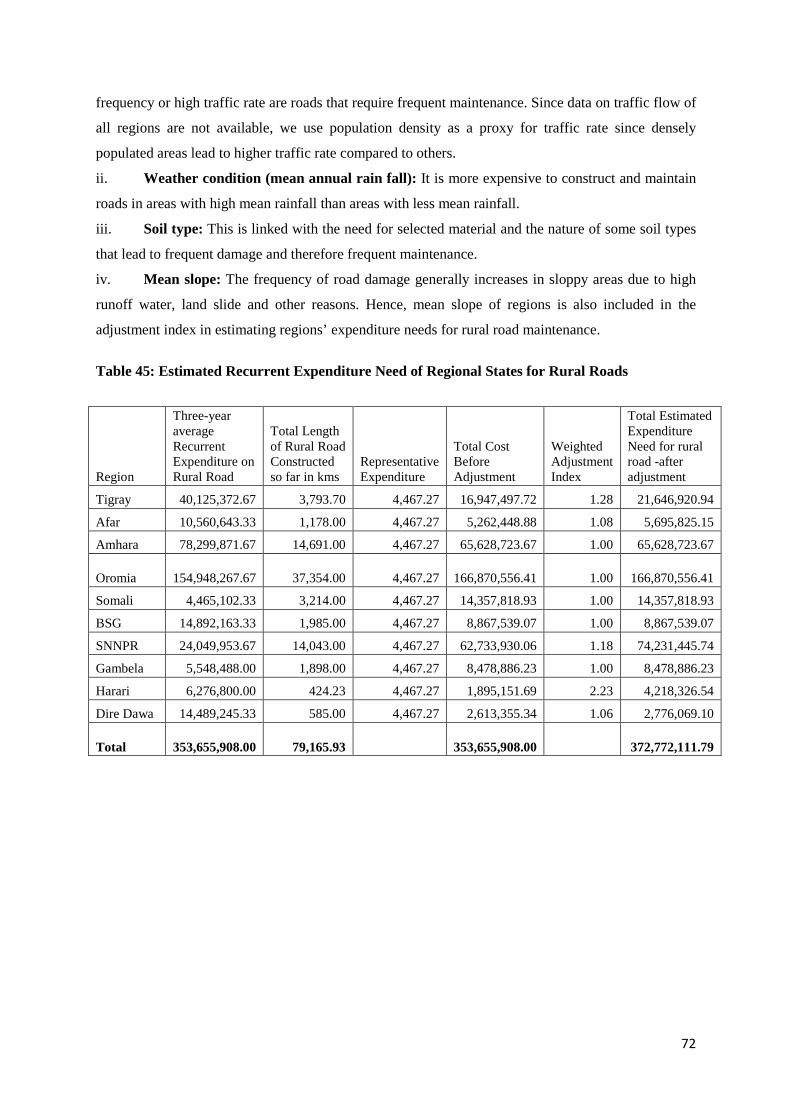
72

frequency or high traffic rate are roads that require frequent maintenance. Since data on traffic flow of

all regions are not available, we use population density as a proxy for traffic rate since densely

populated areas lead to higher traffic rate compared to others.

ii. Weather condition (mean annual rain fall): It is more expensive to construct and maintain

roads in areas with high mean rainfall than areas with less mean rainfall.

iii. Soil type: This is linked with the need for selected material and the nature of some soil types

that lead to frequent damage and therefore frequent maintenance.

iv. Mean slope: The frequency of road damage generally increases in sloppy areas due to high

runoff water, land slide and other reasons. Hence, mean slope of regions is also included in the

adjustment index in estimating regions’ expenditure needs for rural road maintenance.

Table 45: Estimated Recurrent Expenditure Need of Regional States for Rural Roads

Region

Three-year average Recurrent Expenditure on Rural Road

Total Length of Rural Road Constructed so far in kms

Representative Expenditure

Total Cost Before Adjustment

Weighted Adjustment Index

Total Estimated Expenditure Need for rural road -after adjustment

Tigray 40,125,372.67 3,793.70 4,467.27 16,947,497.72 1.28 21,646,920.94

Afar 10,560,643.33 1,178.00 4,467.27 5,262,448.88 1.08 5,695,825.15

Amhara 78,299,871.67 14,691.00 4,467.27 65,628,723.67 1.00 65,628,723.67

Oromia

154,948,267.67 37,354.00 4,467.27

166,870,556.41 1.00

166,870,556.41

Somali 4,465,102.33 3,214.00 4,467.27 14,357,818.93 1.00 14,357,818.93

BSG 14,892,163.33 1,985.00 4,467.27 8,867,539.07 1.00 8,867,539.07

SNNPR 24,049,953.67 14,043.00 4,467.27 62,733,930.06 1.18 74,231,445.74

Gambela 5,548,488.00 1,898.00 4,467.27 8,478,886.23 1.00 8,478,886.23

Harari 6,276,800.00 424.23 4,467.27 1,895,151.69 2.23 4,218,326.54

Dire Dawa 14,489,245.33 585.00 4,467.27 2,613,355.34 1.06 2,776,069.10

Total

353,655,908.00 79,165.93

353,655,908.00

372,772,111.79

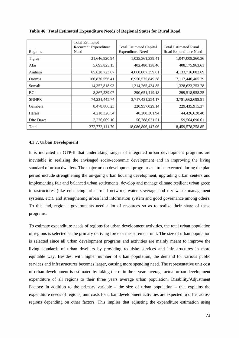
73

Table 46: Total Estimated Expenditure Needs of Regional States for Rural Road

4.3.7. Urban Development

It is indicated in GTP-II that undertaking ranges of integrated urban development programs are

inevitable in realizing the envisaged socio-economic development and in improving the living

standard of urban dwellers. The major urban development programs set to be executed during the plan

period include strengthening the on-going urban housing development, upgrading urban centers and

implementing fair and balanced urban settlements, develop and manage climate resilient urban green

infrastructures (like enhancing urban road network, water sewerage and dry waste management

systems, etc.), and strengthening urban land information system and good governance among others.

To this end, regional governments need a lot of resources so as to realize their share of these

programs.

To estimate expenditure needs of regions for urban development activities, the total urban population

of regions is selected as the primary deriving force or measurement unit. The size of urban population

is selected since all urban development programs and activities are mainly meant to improve the

living standards of urban dwellers by providing requisite services and infrastructures in more

equitable way. Besides, with higher number of urban population, the demand for various public

services and infrastructures becomes larger, causing more spending need. The representative unit cost

of urban development is estimated by taking the ratio three years average actual urban development

expenditure of all regions to their three years average urban population. Disability/Adjustment

Factors: In addition to the primary variable – the size of urban population – that explains the

expenditure needs of regions, unit costs for urban development activities are expected to differ across

regions depending on other factors. This implies that adjusting the expenditure estimation using

Regions

Total Estimated Recurrent Expenditure Need

Total Estimated Capital Expenditure Need

Total Estimated Rural Road Expenditure Need

Tigray 21,646,920.94 1,025,361,339.41 1,047,008,260.36

Afar 5,695,825.15 402,480,138.46 408,175,963.61

Amhara 65,628,723.67 4,068,087,359.01 4,133,716,082.69

Oromia 166,870,556.41 6,950,575,849.38 7,117,446,405.79

Somali 14,357,818.93 1,314,265,434.85 1,328,623,253.78

BG 8,867,539.07 290,651,419.18 299,518,958.25

SNNPR 74,231,445.74 3,717,431,254.17 3,791,662,699.91

Gambela 8,478,886.23 220,957,029.14 229,435,915.37

Harari 4,218,326.54 40,208,301.94 44,426,628.48

Dire Dawa 2,776,069.10 56,788,021.51 59,564,090.61

Total 372,772,111.79 18,086,806,147.06 18,459,578,258.85

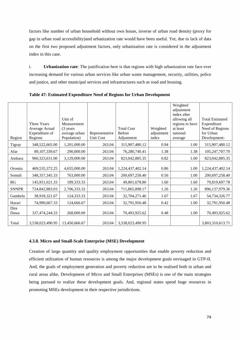
74

factors like number of urban household without own house, inverse of urban road density (proxy for

gap in urban road accessibility)and urbanization rate would have been useful. Yet, due to lack of data

on the first two proposed adjustment factors, only urbanization rate is considered in the adjustment

index in this case.

i. Urbanization rate: The justification here is that regions with high urbanization rate face ever

increasing demand for various urban services like urban waste management, security, utilities, police

and justice, and other municipal services and infrastructures such as road and housing.

Table 47: Estimated Expenditure Need of Regions for Urban Development

4.3.8. Micro and Small-Scale Enterprise (MSE) Development

Creation of large quantity and quality employment opportunities that enable poverty reduction and

efficient utilization of human resources is among the major development goals envisaged in GTP-II.

And, the goals of employment generation and poverty reduction are to be realized both in urban and

rural areas alike. Development of Micro and Small Enterprises (MSEs) is one of the main strategies

being pursued to realize these development goals. And, regional states spend huge resources in

promoting MSEs development in their respective jurisdictions.

Region

Three Years Average Actual Expenditure of Regions

Unit of Measurement (3 years average urban Population)

Representative Unit Cost

Total Cost Before Adjustment

Weighted adjustment index

Weighted adjustment index after allowing all regions to have at least national average

Total Estimated Expenditure Need of Regions for Urban Development-

Tigray 348,522,665.00 1,201,000.00 263.04 315,907,480.12 0.94 1.00 315,907,480.12

Afar 89,107,339.67 290,000.00 263.04 76,280,740.41 1.38 1.38 105,247,707.70

Amhara 960,323,631.00 3,129,000.00 263.04 823,042,885.35 0.82 1.00 823,042,885.35

Oromia 469,535,372.25 4,655,000.00 263.04

1,224,437,402.14 0.86 1.00

1,224,437,402.14

Somali 348,357,345.33 763,000.00 263.04 200,697,258.40 0.56 1.00 200,697,258.40

BG 145,951,021.33 189,333.33 263.04 49,801,678.80 1.60 1.60 79,819,697.78

SNNPR 724,842,883.03 2,706,333.33 263.04 711,865,898.17 1.26 1.26 896,137,979.36

Gambela 38,918,321.67 124,333.33 263.04 32,704,271.46 1.67 1.67 54,734,326.77

Harari 74,990,667.33 124,666.67 263.04 32,791,950.48 0.42 1.00 32,791,950.48 Dire Dawa 337,474,244.33 268,000.00 263.04 70,493,925.62 0.48 1.00 70,493,925.62

Total

3,538,023,490.95

13,450,666.67 263.04

3,538,023,490.95

3,803,310,613.71

75

In estimating regional states’ expenditure need for SMEs development, the size of youth

unemployment (age 15-34) is used as the measurement unit (i.e. major determinant factor of SMEs

development expenditure need). Youth unemployment (age 15-34 ) is chosen on the ground that

regions with large size of unemployed youth need more resources in creating more job opportunities.

The unemployed youth is taken to mean both rural and urban youth as long as the CSA data allow.

In estimating regional states’ expenditure need for MSEs development, representative/standard unit

cost of employment creation is determined as the ratio of recent three years (2005-2007 E.C)average

expenditure data of all regions under consideration for MSEs development to the average number of

employment created by these regions over the same period.

Disability/Adjustment Factors: To take into account the unit cost differential of creating job across

regions, an adjustment is made using the following disability/adjustment factors.

i. Youth illiteracy rate: Regions with high youth literacy rate spend fewer resources on

training youth and prepare the youth for paid employment or self-employment than those with low

youth literacy rate.

ii. Overall unemployment rate: Regions with high over all unemployment rates need to create

more jobs and spend more resources than regions with low over all unemployment rates.

Though including other adjustment factors like proportion of population without electricity and access

to market center would have been useful to account for the ease or difficulty of creating job

opportunity, these factors are not considered in estimating Regions’ SME expenditure need due to

lack of data.

76

Table 48: Estimated Expenditure Needs for MSE development

Region

Three Years Ave.Acutal Expenditure of Regions on SME Dev't (2005-2007 EC)

Average Size of Unemployed Youth Age 15-34

Representative Expenditure

Total Exp.Need for SME Dev't- before adjustment

Weighted Adjustment Indices after allowing all regions to have at least the minimum national average

Total Expenditure Need for SME Development-after adjustment

Tigray 89,481,020.80 115,423.39 597.87 69,007,737.20 1.00 69,007,737.20

Afar 9,594,395.28 49,976.02 597.87 29,878,972.76 1.36 40,497,009.40

Amhara

195,868,592.19 336,566.96 597.87

201,221,993.70 1.00

201,221,993.70

Oromia

379,125,328.49 469,363.90 597.87

280,616,793.30 1.00

280,616,793.30

Somali 60,524,248.61 122,497.89 597.87 73,237,343.12 1.06 77,962,906.42

BSG 1,395,755.43 12,596.18 597.87 7,530,831.76 1.00 7,530,831.76

SNNPR

174,513,036.00 313,790.61 597.87

187,604,790.08 1.00

187,604,790.08

Gambela 12,689,180.74 8,278.99 597.87 4,949,728.80 1.00 4,949,728.80

Harari 17,387,777.70 8,595.44 597.87 5,138,923.56 1.37 7,028,413.38

Dire Dawa 24,135,710.33 26,895.35 597.87 16,079,821.66 2.25 36,138,045.72

Total

964,715,045.56

1,463,984.74

875,266,935.94

912,558,249.76

77

Table 49: Total Expenditure Needs of Regional States before adjustment for Spatial Price Differences

Regions

Administration and General

Services Education Health Agriculture Drinking Water Rural Road Urban

Development MSE

Total Expenditure Need before

Adjustment for Spatial Price

variation

Tigray 1,816,193,211.47 1,063,099,832.94 684,611,426.03 487,988,419.53 905,226,452.57 1,047,008,260.36 315,907,480.12 69,007,737.20 6,389,042,820.21

Afar 761,047,041.86 351,688,951.69 226,225,534.97 580,706,916.48 146,625,371.58 408,175,963.61 105,247,707.70 40,497,009.40 2,620,214,497.29

Amhara 6,060,547,064.43 4,104,429,840.29

2,080,828,074.24

1,563,060,720.00

1,575,889,753.00 4,133,716,082.69 823,042,885.35

201,221,993.70

20,542,736,413.70

Oromia 9,557,656,438.59 7,361,727,782.88

3,370,091,328.00

2,606,859,840.00

2,208,520,425.93 7,117,446,405.79

1,224,437,402.14

280,616,793.30

33,727,356,416.63

Somali 3,233,991,748.16 1,181,425,575.49 545,069,232.00

1,097,950,628.40 357,199,960.01 1,328,623,253.78 200,697,258.40 77,962,906.42 8,022,920,562.65

BG 357,936,347.85 219,951,391.96 221,814,475.60 153,611,887.00 71,912,702.80 299,518,958.25 79,819,697.78 7,530,831.76 1,412,096,293.01

SNNPR 5,408,478,174.26 4,265,682,085.81

1,977,650,870.27

1,400,648,773.33

1,200,424,256.46 3,791,662,699.91 896,137,979.36

187,604,790.08

19,128,289,629.49

Gambela 337,961,144.18 102,066,810.45 113,325,195.44 119,244,409.56 48,511,162.16 229,435,915.37 54,734,326.77 4,949,728.80 1,010,228,692.73

Harari 64,860,920.63 66,455,044.17 55,208,712.63 24,700,313.37 29,610,445.28 44,426,628.48 32,791,950.48 7,028,413.38 325,082,428.43

Dire Dawa 218,201,765.98 128,053,333.18 158,040,717.85 33,681,533.70 60,364,165.37 59,564,090.61 70,493,925.62 36,138,045.72 764,537,578.05

Total

27,816,873,857.42

18,844,580,648.86

9,432,865,567.04

8,068,453,441.39

6,604,284,695.15

18,459,578,258.85

3,803,310,613.71

912,558,249.76

93,942,505,332.18

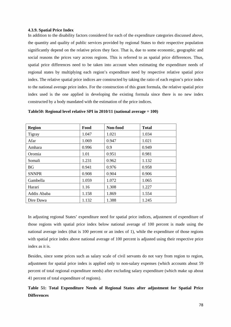
78

4.3.9. Spatial Price Index In addition to the disability factors considered for each of the expenditure categories discussed above,

the quantity and quality of public services provided by regional States to their respective population

significantly depend on the relative prices they face. That is, due to some economic, geographic and

social reasons the prices vary across regions. This is referred to as spatial price differences. Thus,

spatial price differences need to be taken into account when estimating the expenditure needs of

regional states by multiplying each region’s expenditure need by respective relative spatial price

index. The relative spatial price indices are constructed by taking the ratio of each region’s price index

to the national average price index. For the construction of this grant formula, the relative spatial price

index used is the one applied in developing the existing formula since there is no new index

constructed by a body mandated with the estimation of the price indices.

Table50: Regional level relative SPI in 2010/11 (national average = 100)

In adjusting regional States’ expenditure need for spatial price indices, adjustment of expenditure of

those regions with spatial price index below national average of 100 percent is made using the

national average index (that is 100 percent or an index of 1), while the expenditure of those regions

with spatial price index above national average of 100 percent is adjusted using their respective price

index as it is.

Besides, since some prices such as salary scale of civil servants do not vary from region to region,

adjustment for spatial price index is applied only to non-salary expenses (which accounts about 59

percent of total regional expenditure needs) after excluding salary expenditure (which make up about

41 percent of total expenditure of regions).

Table 51: Total Expenditure Needs of Regional States after adjustment for Spatial Price

Differences

Region Food Non-food Total Tigray 1.047 1.021 1.034 Afar 1.069 0.947 1.021 Amhara 0.996 0.9 0.949 Oromia 1.01 0.951 0.981 Somali 1.231 0.962 1.132 BG 0.941 0.976 0.958 SNNPR 0.908 0.904 0.906 Gambella 1.059 1.072 1.065 Harari 1.16 1.308 1.227 Addis Ababa 1.158 1.869 1.554 Dire Dawa 1.132 1.388 1.245

79

Total Expenditure Need before

Adjustment for Spatial Price

variation

Spatial Price Index

Total Expenditure Need net of Salary

Expenses (59 percent)

Non-salary Expenses

Adjusted for Spatial Price

Variation

Salary Expenses (41 percent of total Expenses

Total Estimated Expenditure Needs of Regional States

6,389,042,820.21 1.034 3,769,535,263.93 3,897,699,462.90 2,619,507,556.29 6,517,207,019.19

2,620,214,497.29 1.021 1,545,926,553.40 1,578,391,011.02 1,074,287,943.89 2,652,678,954.91

20,542,736,413.70 0.949

12,120,214,484.08

12,120,214,484.08 8,422,521,929.62 20,542,736,413.70

33,727,356,416.63 0.981

19,899,140,285.81

19,899,140,285.81

13,828,216,130.82 33,727,356,416.63

8,022,920,562.65 1.132 4,733,523,131.97 5,358,348,185.39 3,289,397,430.69 8,647,745,616.07

1,412,096,293.01 0.958 833,136,812.87 833,136,812.87 578,959,480.13 1,412,096,293.01

19,128,289,629.49 0.906

11,285,690,881.40

11,285,690,881.40 7,842,598,748.09 19,128,289,629.49

1,010,228,692.73 1.065 596,034,928.71 634,777,199.07 414,193,764.02 1,048,970,963.09

325,082,428.43 1.227 191,798,632.77 235,336,922.41 133,283,795.66 368,620,718.07

764,537,578.05 1.245 451,077,171.05 561,591,077.96 313,460,407.00 875,051,484.96

93,942,505,332.18

55,426,078,145.99

56,404,326,322.91

38,516,427,186.19 94,920,753,509.11

80

CHAPTER FIVE: TOTAL AND RELATIVE FISCAL GAPS OF REGIONAL STATES

After the expenditure needs are adjusted for spatial price differences, the total annual potential

revenue of each regional State is deducted from the respective total annual expenditure needs to

generate the fiscal gap of each of the grant recipient regional States. The fiscal gap of each of the

regional States is divided to the sum total of the fiscal gap of all regions to obtain the relative fiscal

gaps of each region. The total and relative fiscal gaps of regions are indicated in Table 52.

Table 52: Total and Relative Fiscal Gaps

CHAPTER SIX: CONCLUDING REMARKS AND RECOMMENDATIONS

Region

Total Estimated Expenditure Needs of Regional States

Total Potential Revenue Gap

Relative Gap

Population Share 2007 EC

Tigray 6,517,207,019.19 1,751,924,322.03 4,765,282,697.16 6.03% 5.83%

Afar 2,652,678,954.91 265,716,841.52 2,386,962,113.39 3.02% 1.99%

Amhara 20,542,736,413.70 3,476,076,853.50 17,066,659,560.19 21.60% 23.53%

Oromia 33,727,356,416.63 5,770,358,050.61 27,956,998,366.02 35.38% 38.87%

Somalia 8,647,745,616.07 495,454,951.54 8,152,290,664.53 10.32% 6.29%

BG 1,412,096,293.01 191,850,543.68 1,220,245,749.33 1.54% 1.16%

SNNPR 19,128,289,629.49 2,996,111,089.82 16,132,178,539.66 20.41% 21.08%

Gambela 1,048,970,963.09 177,245,815.48 871,725,147.61 1.10% 0.47%

Harari 368,620,718.07 199,688,218.13 168,932,499.93 0.21% 0.27%

Dire Dawa 875,051,484.96 572,837,420.69 302,214,064.27 0.38% 0.51%

Total 94,920,753,509.11 15,897,264,107.01 79,023,489,402.10 100.00% 100.00%

81

6.1. Conclusions

As stipulated under various articles of the Constitution of the Federal Democratic Republic of

Ethiopia, the federal grant allocation is meant to ensure fiscal equalization, equitable provision of

public services and promote revenue generation capacity of regions/city administration among other

things. Hence, as much as possible, the revision of the grant allocation formula is made objectively

based on a number of core principles such as transparency, adequate stakeholders’ participation,

fairness, understandability/clarity, revenue predictability, and efficiency in revenue generation and

budget utilization, and self-rule and accountability.

Throughout the revision of the grant allocation formula, the research team has worked in close

collaboration with a group of Experts from the Secretariat of the House of Federation. Besides, from

the outset, comprehensive consultative sessions were held with regional government cabinet members

and in-depth discussions conducted with key officials and experts from selected Bureaus/Offices such

as Agricultural and Natural Resource Development Bureau, Health Bureau, Education Bureau,

Finance Bureau and [Rural] Road Development and other Bureaus of each regional State and the City

Administration. These sessions were instrumental in understanding the various concerns of regional

States, in getting their suggestions on the way forward and in gathering some information essential for

the revision of the grant formula. Furthermore, the members of the Standing Committee at the House

of Federation that is mandated with overseeing the revision of the grant formula, representatives from

key regional Bureaus, and other stakeholders have deliberated and agreed on the framework proposed

to revise the grant allocation formula ahead of the revision process (that is, before the revenue and

expenditure estimation process started). Then, draft federal grant allocation formula is prepared as per

the agreement and the directions given by HoF Standing Committee were presented to the members of

the Committee for feedback. The revised grant formula document is then finalized after incorporating

the essential inputs/comments obtained at various stages of the process.

The revision of grant allocation formula is made primarily by using the data obtained from several

federal institutions like CSA, Ministerial offices and other pertinent federal agencies. The research

team in collaboration with HoF experts/staffs exerted utmost effort to address the various concerns

raised by regional States during the revision processes. Despite the efforts made, lack of adequate and

quality data on some essential variables of interest has been one of the most important challenges

faced while estimating revenue generating capacity and expenditure needs of regional States. For

instance, absence of pre-studied tax bases and revenue potential of regions (including joint revenue

potential), total absence of data on some expenditure categories like environmental protection and

inconsistency of data were among the ranges of data related constraints faced. Moreover, it was

impossible to capture some of the concerns raised by regional states like variation in quality of public

82

services provided and efficiency differentials across regional States in this revision. On other hand,

the desire to address many issues using a single federal grant has made the revision process so

challenging.

In light of the aforementioned constraints and other challenges faced during the revision of the

Federal General Purpose Grant Allocation Formula, the following recommendations are forwarded for

future actions.

i) Since data shortage and quality has been one of the single most important challenges, the HoF,

CSA, concerned Federal Institutions as well as regional bureaus need to enhance their data

collection/recording and management practices. Besides, periodically updating data records and cross-

checking with the sources is necessary in improving data quality at all levels. The HoF also needs to

strengthen its internal data management capacity.

ii) Availability of some essential national data/information like pre-assessment of revenue/tax/

potential of regions (including joint revenue) and clearly defined tax base and rate, gap in various

public services versus national standards is essential in undertaking such revision. Hence, the HoF in

collaboration with other concerned offices need to undertake an assessment on such matters so at to

generate better information for future revision of grant allocation formula,

iii) Efficient utilization of allocated grant is important in realizing the purposes that the grant is meant

to serve. To this end, mechanisms to ensure proper utilization of the allocated budget have to be in

place by HoF in a manner that would not jeopardize regional mandate.

iv) As it could be difficult to address too many issues using a single general-purpose grant, it might be

advisable to have some additional specific purpose grants for some issues like security, environmental

pollution.

v) It also seems important that HoF strengthens the capacity of its experts in both exposing its experts

to theoretical foundations of fiscal federalism, different approaches (and their merits and demerits) of

intergovernmental fiscal transfers, and the technical aspects of constructing/revising grant formulas.

This will enable HoF to conduct assessments on grant formulas in a continuous basis that once in

three or five years.

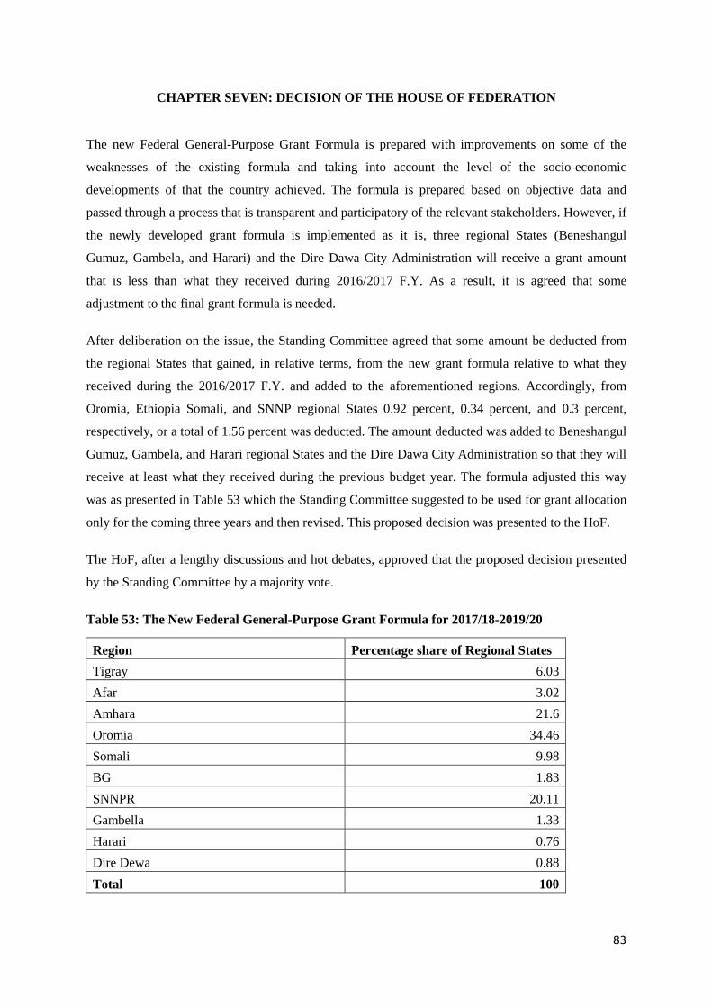
83

CHAPTER SEVEN: DECISION OF THE HOUSE OF FEDERATION

The new Federal General-Purpose Grant Formula is prepared with improvements on some of the

weaknesses of the existing formula and taking into account the level of the socio-economic

developments of that the country achieved. The formula is prepared based on objective data and

passed through a process that is transparent and participatory of the relevant stakeholders. However, if

the newly developed grant formula is implemented as it is, three regional States (Beneshangul

Gumuz, Gambela, and Harari) and the Dire Dawa City Administration will receive a grant amount

that is less than what they received during 2016/2017 F.Y. As a result, it is agreed that some

adjustment to the final grant formula is needed.

After deliberation on the issue, the Standing Committee agreed that some amount be deducted from

the regional States that gained, in relative terms, from the new grant formula relative to what they

received during the 2016/2017 F.Y. and added to the aforementioned regions. Accordingly, from

Oromia, Ethiopia Somali, and SNNP regional States 0.92 percent, 0.34 percent, and 0.3 percent,

respectively, or a total of 1.56 percent was deducted. The amount deducted was added to Beneshangul

Gumuz, Gambela, and Harari regional States and the Dire Dawa City Administration so that they will

receive at least what they received during the previous budget year. The formula adjusted this way

was as presented in Table 53 which the Standing Committee suggested to be used for grant allocation

only for the coming three years and then revised. This proposed decision was presented to the HoF.

The HoF, after a lengthy discussions and hot debates, approved that the proposed decision presented

by the Standing Committee by a majority vote.

Table 53: The New Federal General-Purpose Grant Formula for 2017/18-2019/20

Region Percentage share of Regional States Tigray 6.03 Afar 3.02 Amhara 21.6 Oromia 34.46 Somali 9.98 BG 1.83 SNNPR 20.11 Gambella 1.33 Harari 0.76 Dire Dewa 0.88 Total 100

84

References

Barati, I., and Szalai, A. (2000) Fiscal Decentralization in Hungary. Centre for Public Affairs Studies, Budapest University of Economic Sciences.

Boadway, R. and Shah, A. (2007) Intergovernmental Fiscal Transfers: Principles and Practice. Public

Sector Governance and Accountability Series, the World Bank.

Boadway, Robin (2002a) Revisiting Equalization Again: Representative Tax System vs. Macro Approaches.Working Paper, Institute of Intergovernmental Relations, Queen’s University, Kingston, Ontario, Canada.

Boadway, Robin (2004) The Theory and Practice of Equalization.CESifo Economic Studies 50 (1): 211–54.

Ethiopian Legal Brief: A Blog about Ethiopian Law (2011) “Federal Laws [Federal Laws Year Index,

Council of Minister Regulations, Codes, Directives, Constitutions, and Revised Constitutions

of Regional States]”, Federal NegaritGazeta(several issues). Available at:

http://chilot.me/federal-laws

Fiscal Equalization Transfers.World Bank Policy Research Working Paper 3785, Washington, DC.

House of Federation (2012)The Federal Budget Grant Distribution Formula 2012/13 - 2016/17. Addis

Ababa, Ethiopia

Ma, Jun (1997) Intergovernmental Fiscal Transfers in Nine Countries: Lessons for Developing

Countries. Policy Research Working Paper 1822, The World Bank, Washington, D.C.

Martinez-Vazquez,J. and Timofeev,A.(2010)Technical note on the methodology for the allocation of

intergovernmental grants in the Republic of Belarus. The World Bank, Washington, DC.

MOFED (2014) “Growth and Transformation Plan Annual Progress Report for F.Y. 2012/13”, Addis

Ababa, Ethiopia.

Rafuse, Robert W. (1990) Representative Expenditures: Addressing the Neglected Dimension of

Fiscal Capacity. Advisory Commission on Intergovernmental Relations, Washington, D.C.

Rosen, Harvey S. 2005. Public Finance. 7th ed. Boston: McGraw-Hill/Irwin.

Shah, Anwar (1994) A Fiscal Needs Approach to Equalization Transfers in a Decentralized

Federation. Policy Research Working Paper 1289, The World Bank, Washington, D.C.

Shah, Anwar (1996) A Fiscal Needs Approach to Equalization. Canadian Public Policy – Analyse de

Politiques, XXii: 2: 99-115.

Shah, Anwar (2005b) On Getting the Giant to Kneel: Approaches to a Change in the Bureaucratic

Culture.In Fiscal Management, ed. Anwar Shah, 211–27. Washington, DC: World Bank.

Shah, Anwar (2005a) A Framework for Evaluating Alternate Institutional Arrangements for.

FDRE Proclamation No.1/1995 ‘Proclamation of the Constitution of the Federal Democratic Republic

of Ethiopia’, Federal NegaritGezeta of the Federal Democratic Republic of Ethiopia, 1st year,

No.1, 21st August,1995, Addis Ababa, Ethiopia.

85

FDRE Proclamation No. 416/2004 ‘the Dire-Dawa Administration Charter Proclamation’ Federal

NegaritGezeta of the Federal Democratic Republic of Ethiopia, 10thYear No. 60,30th

July,2004, Addis Ababa, Ethiopia