feature selection for chemical sensor arrays using mutual...

Feature selection for chemical sensor arrays using mutual information

Article (Published Version)

http://sro.sussex.ac.uk

Wang, X Rosalind, Lizier, Joseph T, Nowotny, Thomas, Berna, Amalia Z, Prokopenko, Mikhail and Trowell, Stephen C (2014) Feature selection for chemical sensor arrays using mutual information. PLoS ONE, 9 (3). e89840. ISSN 1932-6203

This version is available from Sussex Research Online: http://sro.sussex.ac.uk/49383/

This document is made available in accordance with publisher policies and may differ from the published version or from the version of record. If you wish to cite this item you are advised to consult the publisher’s version. Please see the URL above for details on accessing the published version.

Copyright and reuse: Sussex Research Online is a digital repository of the research output of the University.

Copyright and all moral rights to the version of the paper presented here belong to the individual author(s) and/or other copyright owners. To the extent reasonable and practicable, the material made available in SRO has been checked for eligibility before being made available.

Copies of full text items generally can be reproduced, displayed or performed and given to third parties in any format or medium for personal research or study, educational, or not-for-profit purposes without prior permission or charge, provided that the authors, title and full bibliographic details are credited, a hyperlink and/or URL is given for the original metadata page and the content is not changed in any way.

http://sro.sussex.ac.uk/

Feature Selection for Chemical Sensor Arrays UsingMutual Information

X. Rosalind Wang1*, Joseph T. Lizier1, Thomas Nowotny2,3, Amalia Z. Berna3, Mikhail Prokopenko1,

Stephen C. Trowell3

1CSIRO Computational Informatics, Epping, NSW, Australia, 2CCNR, School of Engineering and Informatics, University of Sussex, Falmer, Brighton United Kingdom,

3CSIRO Ecosystem Sciences and Food Futures Flagship, Canberra, ACT, Australia

Abstract

We address the problem of feature selection for classifying a diverse set of chemicals using an array of metal oxide sensors.Our aim is to evaluate a filter approach to feature selection with reference to previous work, which used a wrapperapproach on the same data set, and established best features and upper bounds on classification performance. We selectedfeature sets that exhibit the maximal mutual information with the identity of the chemicals. The selected features closelymatch those found to perform well in the previous study using a wrapper approach to conduct an exhaustive search of allpermitted feature combinations. By comparing the classification performance of support vector machines (using featuresselected by mutual information) with the performance observed in the previous study, we found that while our approachdoes not always give the maximum possible classification performance, it always selects features that achieve classificationperformance approaching the optimum obtained by exhaustive search. We performed further classification using theselected feature set with some common classifiers and found that, for the selected features, Bayesian Networks gave thebest performance. Finally, we compared the observed classification performances with the performance of classifiers usingrandomly selected features. We found that the selected features consistently outperformed randomly selected features forall tested classifiers. The mutual information filter approach is therefore a computationally efficient method for selectingnear optimal features for chemical sensor arrays.

Citation: Wang XR, Lizier JT, Nowotny T, Berna AZ, Prokopenko M, et al. (2014) Feature Selection for Chemical Sensor Arrays Using Mutual Information. PLoSONE 9(3): e89840. doi:10.1371/journal.pone.0089840

Editor: James P. Brody, University of California, Irvine, United States of America

Received July 16, 2013; Accepted January 28, 2014; Published March 4, 2014

Copyright: � 2014 Wang et al. This is an open-access article distributed under the terms of the Creative Commons Attribution License, which permitsunrestricted use, distribution, and reproduction in any medium, provided the original author and source are credited.

Funding: This research is supported by the Science and Industry Endowment Fund (http://www.sief.org.au). The funders had no role in study design, datacollection and analysis, decision to publish, or preparation of the manuscript.

Competing Interests: The authors have declared that no competing interests exist.

* E-mail: [email protected]

Introduction

Feature selection is becoming increasingly important with the

rapid increase in the speed and dimensionality of data acquisition

in many fields. Typical application areas include for example

sensor networks [1,2], robotics [3,4], astronomy [5] and bioinfor-

matics [6]. Feature selection is the act of reducing the dimension-

ality of the data — be it from a sensor that collects a vast number

of data points per sample, or data collected in parallel with many

different sensors at the same time — to find the most useful subset

of data for tasks such as classification, navigation or diagnostics.

In this paper, we focus on the problem of feature selection for

classifying chemicals using an array of chemical sensors in an

electronic nose. Our aim is to use an information-theoretic

approach to feature selection (a filter method) on a data set with a

large number of chemicals measured by an electronic nose.

Previous work on feature selection with the same data set by

Nowotny et al. [7] searched for the feature set with the best

classification performance exhaustively (a wrapper method). We

provide a direct comparison between the two approaches to

feature selection and verify the classification performances of the

selected feature sets. In other words, we evaluate the performance

of our efficient filter method of feature selection using the upper

limits provided by the exhaustive wrapper method search.

When selecting sensors for an electronic nose, the major

considerations are the type and number of sensors to use, how to

sample data from the chosen sensors and how to pre-process the

collected raw data (see [8] for a recent review). Recent advances in

solid-state chemistry using combinatorial synthetic approaches [9]

or biosensor design based on natural genetic diversity [10], are

now affording us an almost limitless repertoire of potential

chemical sensors. It is therefore becoming increasingly important

to identify optimal or at least sufficiently good subsets of potential

sensors for incorporation into chemical sensor arrays (see [8,11]

for recent reviews).

An important aspect of the feature selection problem is that the

optimal selection typically depends strongly on each particular

application. It is therefore important to identify methods for

feature selection that maximise the value of the information obtained for

reliable and acceptably-accurate classification, rather than maximising

information per se. The ultimate goal is to optimise classification

accuracy at acceptable cost, which might be the price of sensors,

communication costs, cost of processing and using the data, and

any additional operation cost (e.g. [12]). The aspect of cost is,

however, largely beyond the scope of this paper and will be

considered in future work.

There are three general categories of feature selection methods:

filter, wrapper, and embedded methods. In a filter method (e.g.

PLOS ONE | www.plosone.org 1 March 2014 | Volume 9 | Issue 3 | e89840

http://creativecommons.org/licenses/by/4.0/

[13–15]), features are selected based on some metrics that directly

characterise those features and the process is independent of the

learning and inference (eg. classification) algorithm. Consequently,

feature selection needs only to be performed once, and different

classifiers can be evaluated, making the filter method very

appealing especially when the evaluation of the classification

method is under consideration. In a wrapper method (e.g. [16,17]),

critical features are selected based on the success of the learning

and inference algorithms. Consequently, the wrapper method

often leads to better inferences as it bases its choice of features

directly on the inference results. However, wrapper methods are in

general much more time consuming (although it is common to

adopt some greedy strategies, such as backward elimination or

forward selection, to alleviate the computational cost [18]) than

filter methods as they require executing learning and inference

algorithms on all possible combinations of features. For example,

the application of an SVM through a wrapper approach in [7] to

the data set discussed here required 2–3 weeks of parallel

computing time on a 70 processor modern supercomputer cluster,

while the feature selection using the filter method took around an

hour on a similar supercomputer cluster. Moreover, the previous

work using the wrapper approach did not even include the use of

separate validation and test sets, which would have further

increased the necessary computation time in crossvalidation. This

lack of a separate validation set adds to the risk of over-fitting in

the wrapper based results.

A third feature selection method is the embedded approach,

where the feature selection is built into the training process of the

classifier (e.g. [19,20]). Thus, the embedded approach is similar to

wrapper method in that it is specific to a given learning algorithm.

However, the embedded approach is more computationally

efficient as it makes better use of available data and avoids

retraining from scratch for every possible combination of the

feature set [18].

In this paper, we aim to evaluate the effectiveness of a filter

approach to feature selection, due to its advantage of reducing

computational cost and independence of the classifier, in

comparison to previous work using a wrapper approach. In the

field of olfactory sensors, various metrics based on signal

processing have been proposed for feature selection via filter

methods: Raman et al. [21] selected the subset using a measure

derived from Fisher’s Linear Discriminant Analysis, Muezzinoglu

et al. [22] explored the use of the squared Mahalanobis distance,

and Vergara et al. [13] computed the frequency responses of the

signals by first calculating the input-output cross-correlations and

then calculating the Fourier Transform of the responses. Feature

selection based on machine learning and artificial intelligence

techniques has also been explored by various groups. Among these

techniques, Genetic Algorithms (GAs) are popular (e.g. [15,23,24])

due to the approach’s resilience to becoming trapped in local

optima. While the studies above showed good classification results

from the feature selection, in most cases only one or two classifiers

were tested. Furthermore none of the studies compared the results

with an exhaustive wrapper-based search of features.

Another approach to filter-based feature selection relies on

information theory. First derived by Shannon [25], information

theory provides a measure of the uncertainty associated with the

data, allowing us to quantify what is meant by ‘‘information

collected by the sensors’’. Consequently, it is a natural measure to

be employed in selecting the best features independently from the

classification methods to be used. Methods based on information

theory have been used quite widely to optimise, for example,

optimal geospatial arrangement of sensor arrays. Krause and

Guestrin [26] introduced a criterion which minimises the

conditional entropy of all the possible sensors given the subset

chosen. These authors also proposed a criterion maximising the

mutual information between the subset and the rest of the sensors

[14]. Olsson et al. [1] suggested a method that uses a combination

of mutual information and information metric to describe an

information coverage (IC), which balances redundancy and

novelty in the data. More recently, Wang et al. [27] explored the

selection of sensors by maximising the entropy in the subsets and

showed, using a simple data set, that the different sensor selection

metrics selected very similar subsets. In all the cases above, the

objective was to select the optimal spatial placement of sensors

such that the maximum amount of data is gathered, the

optimisations were not done for the purpose of classification of

some target variable.

In the field of artificial olfaction, the use of information theory

for optimising a sensor array first appeared a decade ago in a

paper published by Pearce and Sanchez-Montanes [28]. In this

paper, the authors showed that Fisher Information can be used as

a lower bound for the classification performance of the sensor

responses. Vergara et al. [29] optimised the operating temperature

for a single sensor by maximising the Kullback-Leibler distance

(KL-distance) with respect to a single parameter, the sensor heater

voltage, for a given set of odours. The paper compared the results

with that of Mahalanobis distance (MD) and found that the

optimal parameter identified by the KL-distance led to better

classification performance in the considered six-class problem.

Our aim was to evaluate the performance of mutual information

(MI), as an efficient and conceptually relevant filter approach, in

feature selection for a chemical sensor array across a range of

classifiers and in relation to a computationally exhaustive wrapper

approach applied to the same data set in the recent study by

Nowotny et al. [7]. Mutual information is a measure of the amount

of information one random variable contains about another [30].

The MI between two variables tells us the reduction in uncertainty

of one due to the knowledge of the other. In the case of feature

selection, maximising the MI among variables gives us the subset

with the most novel and non-redundant information about the sensor

data (see Methods for full details of the criterion).

The use of mutual information for feature selection in

classification problems was first suggested by Battiti [31]. Recently,

Fonollosa et al. [32] used Mutual Information (MI) to optimise the

operating temperature of four metal-oxide sensors when measur-

ing four different gases at various concentrations. To calculate the

MI, the authors quantised the continuous responses of the sensors.

The authors showed that sensor arrays with different numbers of

sensors have different maximum MI over a range of gas

concentrations. The paper concluded that the MI approach can

be used to quantify the classification abilities of the sensors,

however, no classification results were shown to verify this claim.

It is known that MI from a large set of features with a small

amount of data can be difficult to estimate, and also there can be a

large number of potential feature sets to evaluate [31,33]. Peng et

al. [34] attempted to address these issues by computing minimal-

Redundancy-Maximum-Relevance (mRMR) of candidate features

with the class values. The mRMR algorithm does not consider all

possible features in every size constraint, rather, it iteratively

selects new features by minimising their pairwise redundancy with

features chosen in previous steps and maximises their relevance to

the class, thus reducing the computational cost. The authors

showed that their approach efficiently selects good feature sets for

multiple classification methods in 4 different data sets. Similarly to

the mRMR algorithm, Rodriguez-Lujan et al. [35] formulated the

problem of solving minimum redundancy and maximum rele-

vance for the feature selection of large data sets using a method

Feature Selection Using Mutual Information


named Quadratic Programming Feature Selection (QPFS). The

authors introduced an objective function with quadratic and linear

terms to capture the pairwise dependence between the variables

and novelty between the feature and class. The QPFS algorithm

solves the quadratic programming problem using the Nystrom

method to improve computational speed. The authors showed that

the algorithm can achieve similar accuracy to previous methods

but with higher efficiency. Recently, Pashami et al. [2] modified the

QPFS algorithm by applying the Fisher index, a ratio between the

mean and standard deviation of the samples, to compute the

relevance of the data. The authors applied the modified algorithm

to data from an array of metal oxide gas sensors, similar to those

used in this paper, for the detection of changes in distant gas

sources.

In this paper, we will evaluate MI exhaustively for all potential

feature sets despite the aforementioned issues with its efficient

estimation and with potential computational cost in general. In

contrast to directly estimating MI from the candidate set of

features, the pairwise approaches [34,35] discussed earlier use only

heuristics for minimising redundancy and do not capture synergies

of the features with the class (See Methods for further details).

Addressing redundancy and synergy simultaneously is key in

designing devices with the minimum number of sensors with the

best possible classification performance, and can only be achieved

with a full multivariate evaluation. Also, we use a recently

developed nearest-neighbours technique for estimating MI [36],

which has been demonstrated to be efficient for a relatively large

number of variables. This technique allows us to utilise the full

range of responses of the sensors, which is advantageous over the

quantisation process employed by Fonollosa et al. [32]. Finally, we

have a relatively small number of features, thus the evaluation of

MI for all possible combinations of features is computationally

tractable, aligning with our goal of comparing feature selection via

our best possible MI estimates with the wrapper approach that was

based directly on classification.

Without a direct comparison with mRMR and QPFS we do not

claim that these less computationally intensive algorithms would

significantly under-perform for a given dataset. Therefore, a

choice between (a) a more comprehensive information theoretic

approach advocated in this paper and (b) a simpler pair-wise

approach that alleviates the computational cost of the algorithm

remains an open question. Typically, such a question would need

to be resolved when a particular trade-off between computational

efficiency and classification accuracy can be established for specific

datasets.

Feature selection and subsequent classification was performed

on data from 12 metal oxide sensors used to make 10 replicate

measurements of 20 chemical analytes, each at a fixed concen-

tration. The features to be selected comprise the 12 sensors and 6

candidate time points taken from the 2 Hz data stream generated

during sample presentation. Each combination of an individual

sensor with a candidate time point can be viewed as a virtual

sensor or ‘‘feature’’. This data set is the same as used by Nowotny

et al. [7], who employed a wrapper method to exhaustively search

through all permitted combinations of sensors and time points to

find the best feature sets. Here, we employ a maximum MI

criterion to find feature subsets. We then compare the resulting

feature sets, as well as their classification performance, with those

reported from the exhaustive search in [7]. Finally, we also

perform classification with the selected feature sets using a variety

of common classifiers in addition to the linear support vector

machines used in [7] and compare the results across classifiers.

Results

We evaluate our feature selection method in 10 fold cross

validation. The data set of 200 measurements is randomly split

(many times) into a training set of 180 measurements and a test set

of the remaining 20 measurements. For each such split into a

training and test set, we first identify an optimal feature set using

the training data. These features are then extracted from the full

measurements of both the training and test sets. We then test

numerous different classifiers by training them on the resulting

training data and evaluating them with the test data. The observed

performance of the entire feature selection and classification

process, as well as a comparison to the classification performance

in the exhaustive search in [7], are reported below.

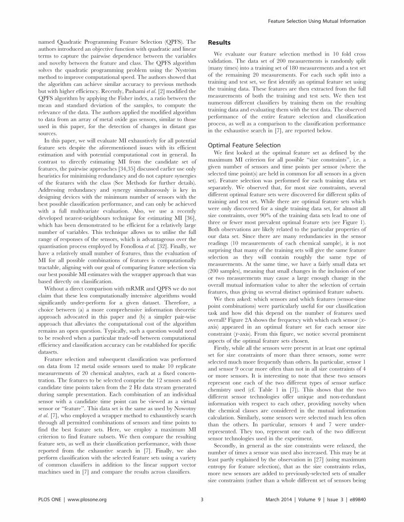
Optimal Feature SelectionWe first looked at the optimal feature set as defined by the

maximum MI criterion for all possible ‘‘size constraints’’, i.e. a

given number of sensors and time points per sensor (where the

selected time point(s) are held in common for all sensors in a given

set). Feature selection was performed for each training data set

separately. We observed that, for most size constraints, several

different optimal feature sets were discovered for different splits of

training and test set. While there are optimal feature sets which

were only discovered for a single training data set, for almost all

size constraints, over 90% of the training data sets lead to one of

three or fewer most prevalent optimal feature sets (see Figure 1).

Both observations are likely related to the particular properties of

our data set. Since there are many redundancies in the sensor

readings (10 measurements of each chemical sample), it is not

surprising that many of the training sets will give the same feature

selection as they will contain roughly the same type of

measurements. At the same time, we have a fairly small data set

(200 samples), meaning that small changes in the inclusion of one

or two measurements may cause a large enough change in the

overall mutual information value to alter the selection of certain

features, thus giving us several distinct optimised feature subsets.

We then asked: which sensors and which features (sensor-time

point combinations) were particularly useful for our classification

task and how did this depend on the number of features used

overall? Figure 2A shows the frequency with which each sensor (x-

axis) appeared in an optimal feature set for each sensor size

constraint (y-axis). From this figure, we notice several prominent

aspects of the optimal feature sets chosen.

Firstly, while all the sensors were present in at least one optimal

set for size constraints of more than three sensors, some were

selected much more frequently than others. In particular, sensor 1

and sensor 9 occur more often than not in all size constraints of 4

or more sensors. It is interesting to note that these two sensors

represent one each of the two different types of sensor surface

chemistry used (cf. Table 1 in [7]). This shows that the two

different sensor technologies offer unique and non-redundant

information with respect to each other, providing novelty when

the chemical classes are considered in the mutual information

calculation. Similarly, some sensors were selected much less often

than the others. In particular, sensors 4 and 7 were under-

represented. They too, represent one each of the two different

sensor technologies used in the experiment.

Secondly, in general as the size constraints were relaxed, the

number of times a sensor was used also increased. This may be at

least partly explained by the observation in [27] (using maximum

entropy for feature selection), that as the size constraints relax,

more new sensors are added to previously-selected sets of smaller

size constraints (rather than a whole different set of sensors being



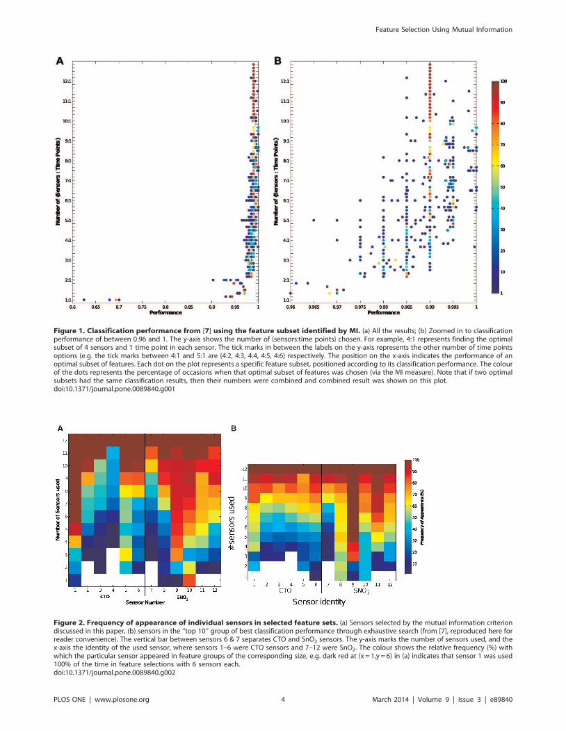
Figure 1. Classification performance from [7] using the feature subset identified by MI. (a) All the results; (b) Zoomed in to classificationperformance of between 0.96 and 1. The y-axis shows the number of {sensors:time points} chosen. For example, 4:1 represents finding the optimalsubset of 4 sensors and 1 time point in each sensor. The tick marks in between the labels on the y-axis represents the other number of time pointsoptions (e.g. the tick marks between 4:1 and 5:1 are {4:2, 4:3, 4:4, 4:5, 4:6} respectively. The position on the x-axis indicates the performance of anoptimal subset of features. Each dot on the plot represents a specific feature subset, positioned according to its classification performance. The colourof the dots represents the percentage of occasions when that optimal subset of features was chosen (via the MI measure). Note that if two optimalsubsets had the same classification results, then their numbers were combined and combined result was shown on this plot.doi:10.1371/journal.pone.0089840.g001

Figure 2. Frequency of appearance of individual sensors in selected feature sets. (a) Sensors selected by the mutual information criteriondiscussed in this paper, (b) sensors in the ‘‘top 10’’ group of best classification performance through exhaustive search (from [7], reproduced here forreader convenience). The vertical bar between sensors 6 & 7 separates CTO and SnO2 sensors. The y-axis marks the number of sensors used, and thex-axis the identity of the used sensor, where sensors 1–6 were CTO sensors and 7–12 were SnO2. The colour shows the relative frequency (%) withwhich the particular sensor appeared in feature groups of the corresponding size, e.g. dark red at (x = 1,y = 6) in (a) indicates that sensor 1 was used100% of the time in feature selections with 6 sensors each.doi:10.1371/journal.pone.0089840.g002



selected at the larger size). This situation would be advantageous

when applying our sensor selection criteria to practical situations:

for example, if a sensor array for detecting a particular disease was

to be manufactured at different costs, then the versions for each

cost of production (i.e. optimised for a different number of sensors)

could be efficiently manufactured by incremental addition of

sensors from within the same (reduced) set of sensors. This

observation can also help with future feature selection problems

when the number of features is so large that evaluating MI for all

possible combinations of features becomes intractable: in such

cases it would be possible to iteratively select new features as the

size constraint increases, knowing that the full feature set for the

new size constraint would likely be the optimal or near-optimal set

if all combinations were evaluated.

Lastly, we notice that the SnO2 sensors are included in the

optimal feature sets more often than the CTO sensors across

almost all size constraints. This is shown in Table 1 where we

calculated the percentage of total optimal feature sets containing

various sensor compositions. From this table, we can see that (for a

given number of sensors) there are always more selected sets where

the SnO2 sensors outnumber the CTO sensors. One possible

reason for the prevalence of the SnO2 sensors could be merely

because they are more sensitive than the CTO sensors (see

Figure 3). However, sensitivity is only one aspect of sensor quality

and may be less important than sensor noise and specificity, when

it comes to analyte classification.

Another interesting observation in Table 1 is that, except for

sensor size constraints with very few sensors, there are no feature

sets where only one type of sensor technology was found in the

optimal feature sets. This is consistent with the observation that

the pair of most and the pair of least frequently used sensors each

contained representatives from both classes of sensor chemistry.

This strengthens the evidence that the two sensor chemistries

provide unique and non-redundant information with respect to

each other.

Figure 4 shows each feature’s frequency of appearance given the

size constraints in both the number of sensors and time points.

This figure gives a finer understanding of the features selected.

Again, we notice several aspects: Firstly, for time point constraints

of 1, over almost all sensor size constraints, time point 2 or 3 (i.e.,

the data gathered at 20 and 30 seconds) is chosen for the optimal

feature sets. From Figure 3, we can see that these are times just

before the maximal responses of the sensors, where we should

expect the maximum amount of variation in the data giving us the

largest values in MI.

The second point of interest was noticed earlier in the sensor

only constraints, that is, in most cases, as the size of time point

constraints increases, more features were added to existing sets.

The exceptions are sensors 3 and 4, which do not get chosen for

time point constraints of more than 4 for many of the sensor

number constraints. This can be explained by looking closely at

the data from these sensors for Tw40s, as the readings from these

sensor hovers just above 0 from this time point onwards. This

means while at small T these two sensors provide information on

the chemicals, they do not provide any information for large T ,

thus they are included in those constraints with a small number of

time points but not for those with a large number.

Comparison with the Wrapper Method of FeatureSelectionThe optimal subsets of features found using our MI criterion

were compared with the results reported in [7]. In both methods,

the SVM cost parameter of C~65536 is used. The authors of [7]

compared classification results of 4 different C values and found

consistent performances, thus report only the performance of the

largest C value. We tested the performance of the linear SVM with

9 different C values (see Methods: Classification Methods), and

found that C~65536 performs better than or consistently with the

other C values (see Figure S1). Therefore, we compare the two

feature selection methods using the same C value.

While both methods use 10 repetitions of ten-fold balanced

cross-validation for measuring classification performance, there is

one subtle difference in the execution: In our method here, for

each of the 100 training sets, we calculate the optimal feature set

using the MI criterion for that training set of 180 data samples and

then use the identified feature set to determine the classification

performance for the corresponding test set of 20 data samples. We

eventually report the average of all observed performances. In the

wrapper approach in [7], classification performance is calculated

across all 100 training and test set splits for each possible

combination of feature sets of a given size constraint. The 10

Table 1. Analysis of the balance between sensors of different chemistry used in selected feature sets.

No. Sensors % CTO only % SnO2 only % CTO.SnO2 % SnO2.CTO % CTO=SnO2

1 14.3 85.7 0.0 0.0 0.0

2 0.0 19.0 0.0 0.0 81.0

3 0.0 2.2 33.7 64.2 0.0

4 0.0 2.0 11.0 52.7 34.3

5 0.0 0.0 17.7 82.3 0.0

6 0.0 0.0 9.0 43.0 48.0

7 0.0 0.0 45.3 54.7 0.0

8 0.0 0.0 35.3 51.5 13.2

9 0.0 0.0 42.2 57.8 0.0

10 0.0 0.0 31.3 52.0 16.7

11 0.0 0.0 38.2 61.8 0.0

12 0.0 0.0 0.0 0.0 100.0

Each row shows the composition of the feature sets selected by MI given the sensor size constraint, the columns give the percentage of the total selected feature setswith the labelled sensor contents.doi:10.1371/journal.pone.0089840.t001



feature sets with the best so determined classification performances

are selected as the optimal feature sets, or the ‘‘top 10’’ group and

their average achieved classification performance is reported. Note

that the reported performances do not include the use of separate

evalutation and test sets and may, therefore, not accurately reflect

the expected performance on entirely new, unseen data, due to the

known risks of overfitting. We display the relevant data from [7] in

Figures 2B and 5 for easy reference and comparison.

First, we compare the sets selected by maximum MI criterion

(Figure 2A) with the ‘‘top ten’’ sensor sets from [7] (Figure 2B).

We notice many similarities between the two figures: (1) The

distribution of the colours is very similar; (2) Sensor 9, which was

the most ‘popular’ sensor in the feature sets from [7] has almost

the identical percentage of appearance in Figure 2A; (3) Sensor 7

was rarely used in both sets of selected features; (4) In Figure 2B,

Sensors 8 and 10 were preferentially used in the very small feature

sets of only one or two sensors, while in our feature sets Sensor 10

was preferred in these size constraints with Sensor 8 preferred to a

comparable but lesser degree.

Furthermore, in [7], the authors noted that ‘‘the best feature sets

typically contain sensors of both the standard SnO2 and zeolite-

coated CTO types’’ and 99.55% of the ‘‘sensor combinations that

allowed 100% performance’’ use ‘‘sensors from both technolo-

gies’’. This is validated by our observation in Table 1 where 90%

of the selected sets contains sensors from both technologies. Note

that this includes sensor size constraint 1 for which the criterion

obviously cannot be fulfilled. If we exclude these cases, we find that

97.89% of the remaining selected sets contain sensors of both

types. When only one type of sensor was used in classification in

[7], the SnO2 sensors have much better performance than the

CTO sensors. This also agrees with the results in Table 1 where (a)

SnO2 sensors were utilised more often than the CTO sensors in

most optimal feature sets, and (b) on those occasions where only

one sensor type was used, SnO2 sensors were chosen 90% of the

times.

The similarities described indicate that the feature sets

discovered here match closely those found by exhaustive search

of classification results.

While the overall patterns between the two figures are similar,

there are also some subtle differences in the frequency of

appearance of the sensors as identified by the two methods: (1)

In [7] Sensor 9 was included in almost all feature sets for size

constraints of 5 or more sensors, whereas in our case it is used less

often (90% of selections) and Sensor 1 assumes the dominant

position. (2) For feature sets of small size constraints, Sensor 8 was

utilised over 50% of the times in [7], while here Sensor 10 was

picked more than 80% of the times. Further, Sensor 1 and 6’s

appearances for size constraint of 1 are swapped. (3) The

percentage of appearance of sensors 10 and 11 in the optimal

feature sets seems to almost switch around between the two

methods, apart from those with very small size constraints. (4)

Sensor 4 was utilised a lot less in the results here than in the ‘‘top

ten’’ sensor sets in [7]. The reasons for these differences are not

obvious but it is interesting to note that sensor 1 has the highest

sensitivity within the group of CTO sensors, even though its signal-

to-noise ratio (SNR) is not particularly good within the group of

CTO sensors and much worse than any of the SnO2 sensors.

Sensor 9, on the other hand, has sensitivity at the lower end of the

SnO2 group, albeit much higher than any of the CTO sensors.

Furthermore, sensor 4 has by far the lowest sensitivity of any

Figure 3. Example FOX Enose responses from the twelve-sensor array. Colour bar on the right shows the sensor number, where 1–6 areCTO sensors and 7–12 are SnO2 sensors. Responses of SnO2 sensors are drawn downwards and responses of CTO sensors upwards. The verticaldashed lines mark the time points where the data for the study was extracted. The sensor readings here show the response to 1-pentanol. Note thatonly the first 100 seconds of the full 300 seconds of data are shown here.doi:10.1371/journal.pone.0089840.g003



sensor even though it has the highest signal-to-noise ratio within

the group of CTO sensors. This dichotomy may be behind the

differential preference for the readings of this sensor in the MI and

wrapper feature selection. In other words, the MI method has a

preference for sensors with high sensitivity (resulting in high

variances in the data), while the wrapper approach prefers those

with high SNR. This difference in preferences of selected sensors

could be due to the linearity of the SVM classifier and the non-

linear nature of the Kraskov-Grassberger technique we employed

in estimating the probability distribution of the data (see Methods).

Having compared the prevalence of sensors and features in the

chosen feature sets we now proceed by examining the classification

results reported in [7] for the features sets that we here selected via

the maximum MI criterion. Figure 1A shows the classification

performance (x-axis) of all the different feature sets against the size

constraints (y-axis), while the frequency with which each feature

set appears in a size constraint is shown by the colour as indicated

by the colour bar. Figure 1B shows the same results for those with

classification performance of greater than 0.96. For comparison,

the classification performance of all the permutations of feature

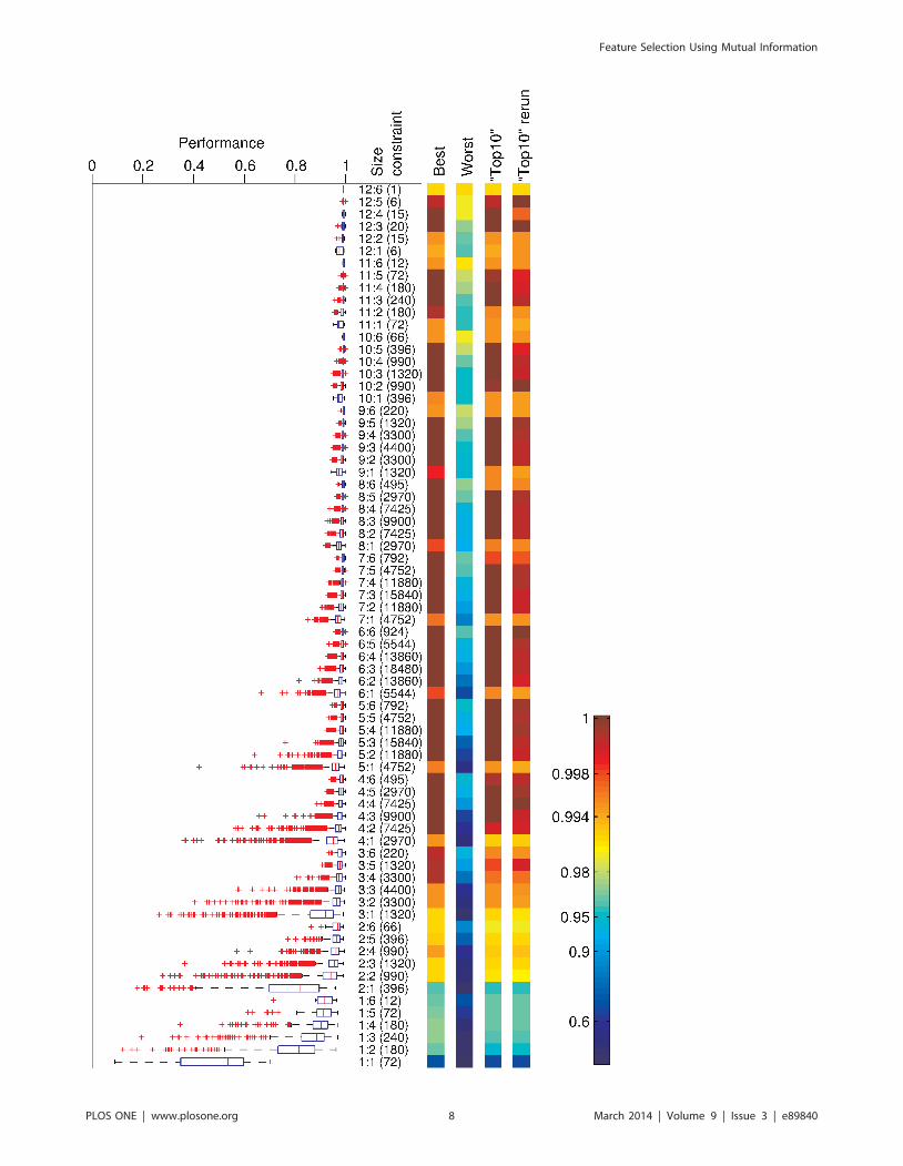
sets is shown in Figure 5.

When comparing the two sets of results, we observe that the

feature sets selected by the maximal MI criterion give close to the

best achievable classification results. All the classification results

from these selected feature sets are above the 75% quantiles shown

in Figure 5. For example, for the size constraint of 1 sensor and 1

data point, the 75% quantile is 0.6 with the best result being 0.7,

the performances in Figure 1 for the constraint are between 0.62

and 0.7. Further, we can see in Figure 1 that the classification

result of the majority of the optimal feature sets selected were very

close to the top performances. In other words, the maximal MI

criterion was able to identify those features that give close to

optimal performances in the classification. This is important, since

as a filter technique it is much more efficient at feature selection

than the exhaustive search of a wrapper method.

Now, we note that while these feature selections did not

necessarily give the very best possible classification performance

(e.g. many of the results in the ‘‘best’’ column in Figure 5 have a

performance of 1), the difference in performance is actually only

about 1 or 2 errors, which is not statistically significant for a data

set of 200 samples. Second, it is important to remember that the

best performances reported in [7] are not a realistic prediction of

what a wrapper approach to feature selection would achieve for

truly new data. A first indication of this is that rerunning the

classification using the ‘‘top 10’’ feature sets with different

training/test set splits in [7] already resulted in slightly worse

performance in general. A true estimate of the performance of a

classifier system with a wrapper approach would only be obtained

if the wrapper method was completed with training and evaluation

sets and the features so identified would then be tested with

separate testing data. Our comparison to the work in [7] should

hence be seen as a comparison to the theoretically best achievable

performance (as identified by the extensive search of a wrapper

method) rather than a comparison to a wrapper method. As such,

we conclude that the maximal MI criterion performs as well as one

could expect from a filter method.

Figure 6 shows the average classification results from [7] of all

the optimal feature sets identified via the maximal MI criterion,

weighted by the number of times each set was chosen in all the

training sets. Comparing these results with the ‘‘top 10’’ column in

Figure 4. Frequency of appearance of individual features in selected feature sets. The y-axis indicates the number of {sensors:time points}used. For example, 4:1 represents finding optimal subset of 4 sensors and 1 time point in each sensor. The rows in between the labels on the y-axisrepresents the other options for the number of time points (e.g. the rows between 4:1 and 5:1 are {4:2, 4:3, 4:4, 4:5, 4:6} respectively. The x-axis marksthe identities of the sensors and time points that were used. Colours represent the frequency (%) with which a {sensor:time point} combination waschosen, as shown in the colour scale.doi:10.1371/journal.pone.0089840.g004



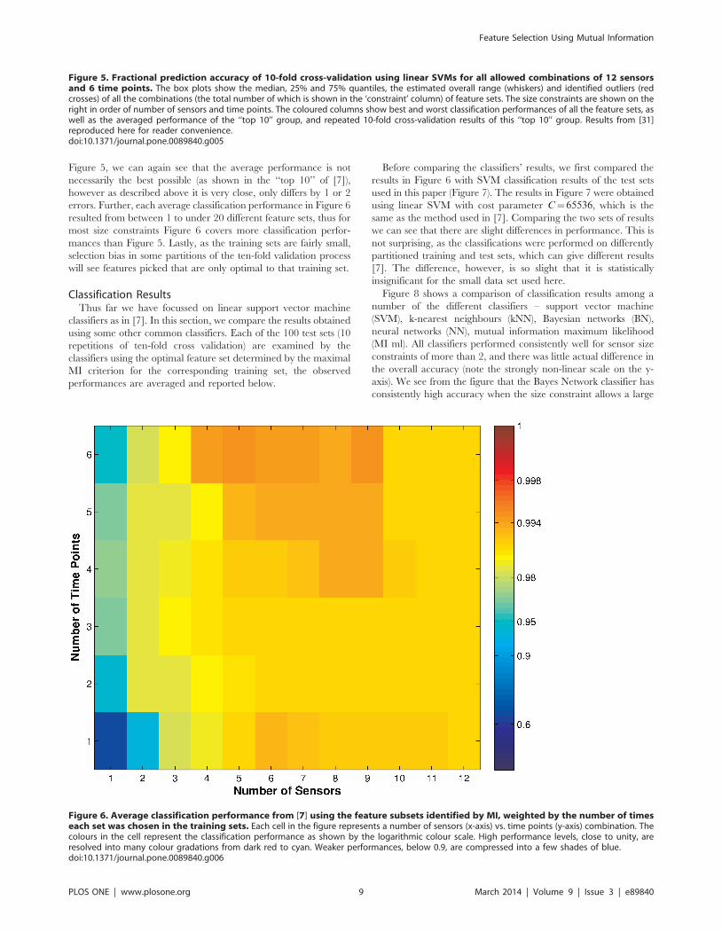
Figure 5, we can again see that the average performance is not

necessarily the best possible (as shown in the ‘‘top 10’’ of [7]),

however as described above it is very close, only differs by 1 or 2

errors. Further, each average classification performance in Figure 6

resulted from between 1 to under 20 different feature sets, thus for

most size constraints Figure 6 covers more classification perfor-

mances than Figure 5. Lastly, as the training sets are fairly small,

selection bias in some partitions of the ten-fold validation process

will see features picked that are only optimal to that training set.

Classification ResultsThus far we have focussed on linear support vector machine

classifiers as in [7]. In this section, we compare the results obtained

using some other common classifiers. Each of the 100 test sets (10

repetitions of ten-fold cross validation) are examined by the

classifiers using the optimal feature set determined by the maximal

MI criterion for the corresponding training set, the observed

performances are averaged and reported below.

Before comparing the classifiers’ results, we first compared the

results in Figure 6 with SVM classification results of the test sets

used in this paper (Figure 7). The results in Figure 7 were obtained

using linear SVM with cost parameter C~65536, which is the

same as the method used in [7]. Comparing the two sets of results

we can see that there are slight differences in performance. This is

not surprising, as the classifications were performed on differently

partitioned training and test sets, which can give different results

[7]. The difference, however, is so slight that it is statistically

insignificant for the small data set used here.

Figure 8 shows a comparison of classification results among a

number of the different classifiers – support vector machine

(SVM), k-nearest neighbours (kNN), Bayesian networks (BN),

neural networks (NN), mutual information maximum likelihood

(MI ml). All classifiers performed consistently well for sensor size

constraints of more than 2, and there was little actual difference in

the overall accuracy (note the strongly non-linear scale on the y-

axis). We see from the figure that the Bayes Network classifier has

consistently high accuracy when the size constraint allows a large

Figure 5. Fractional prediction accuracy of 10-fold cross-validation using linear SVMs for all allowed combinations of 12 sensorsand 6 time points. The box plots show the median, 25% and 75% quantiles, the estimated overall range (whiskers) and identified outliers (redcrosses) of all the combinations (the total number of which is shown in the ‘constraint’ column) of feature sets. The size constraints are shown on theright in order of number of sensors and time points. The coloured columns show best and worst classification performances of all the feature sets, aswell as the averaged performance of the ‘‘top 10’’ group, and repeated 10-fold cross-validation results of this ‘‘top 10’’ group. Results from [31]reproduced here for reader convenience.doi:10.1371/journal.pone.0089840.g005

Figure 6. Average classification performance from [7] using the feature subsets identified by MI, weighted by the number of timeseach set was chosen in the training sets. Each cell in the figure represents a number of sensors (x-axis) vs. time points (y-axis) combination. Thecolours in the cell represent the classification performance as shown by the logarithmic colour scale. High performance levels, close to unity, areresolved into many colour gradations from dark red to cyan. Weaker performances, below 0.9, are compressed into a few shades of blue.doi:10.1371/journal.pone.0089840.g006



number of sensors. To test whether the differences in the

classification performances are statistically significant, we per-

formed two-tailed t-test (see Methods, Equation 2) to compare the

performances at each size constraint between any pair of

classification methods. We found that, for most of the size

constraints, the BN classifier’s performance was superior to that of

the kNN classifier with a p-value Pv0:05. For some size

constraints the BN classifier’s performance is also significantly

superior to the performance of either NN or MI classifiers. There

was effectively no statistically significant difference in performance

between BN and SVM classifiers.

For all the classifiers examined and for each size constraint, we

then compared the performance of the feature sets selected using

the MI criterion against 100 randomly selected feature sets.

Figure 9 shows the average classification results on the data sets for

all the methods using the randomly selected features. Comparing

the two figures, we can see that the classification performances

using features selected by MI are consistently higher than those

using randomly selected features, at all size constraints. Using a

two-tailed t-test (see Methods, equation 2), we found almost all

differences in the performance between MI-selected and random-

ly-selected feature sets are statistically significant at Pv0:05.Therefore, the consistency in the better classification performance

using the features selected by the MI method across all

classification methods shows that the feature selection algorithm

was able to select the subset that was advantageous to the

employed classifiers.

Discussion

Comparison to MI with no constraintsWe formulated the feature selection task by imposing separate

constraints on the number of sensors and the number of time

points in the feature set. A chosen feature combination then uses

the same selected time points for each of the selected sensors. This

constraint on the candidate feature sets greatly reduces the

number of features in the search space, for example, there are

12

6

� �

|6

3

� �

~18480 combinations for 6 sensors and 3 time

points with this constraint, compared to72

18

� �

~4:14|1016

combinations for an arbitrary combination of 18 features when

this constraint is not imposed. However, it is worth noting that the

imposed constraint implies that the feature set with the truly

maximal MI might not be found.

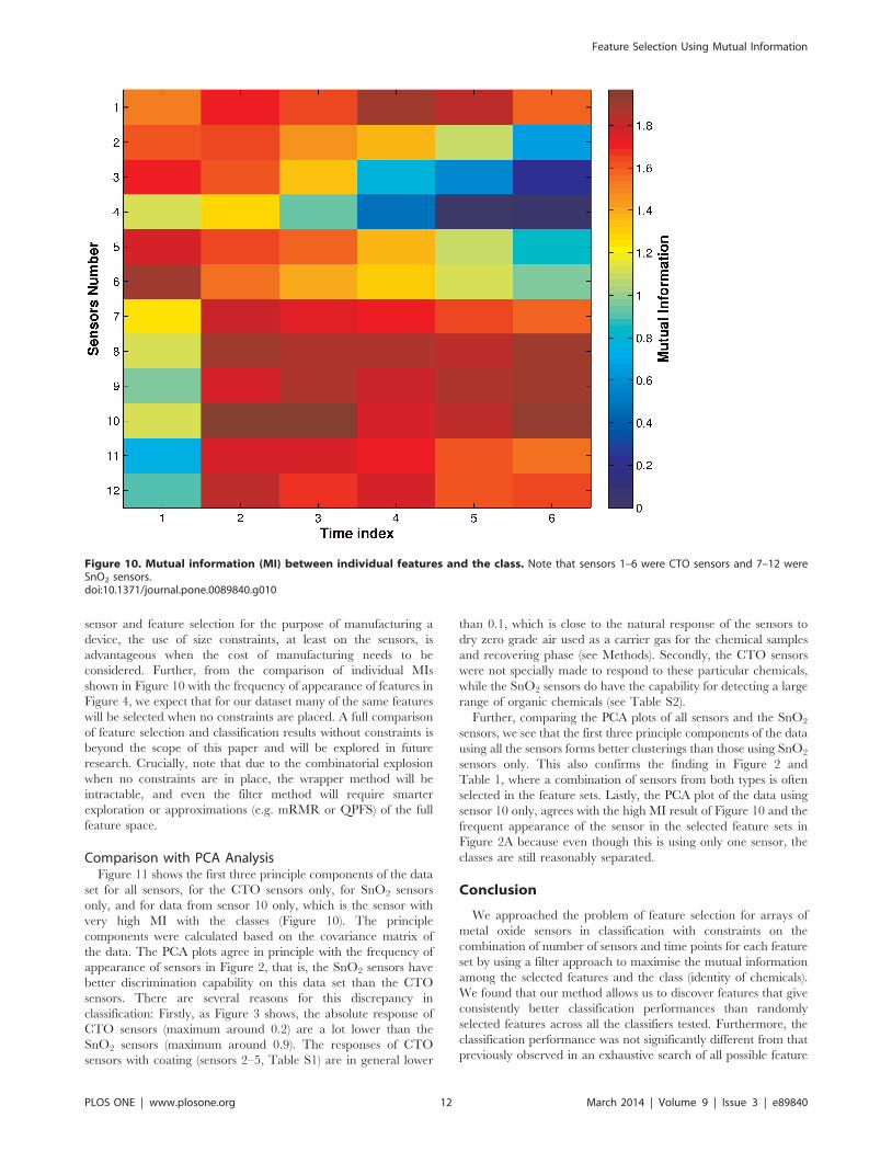
Figure 10 shows the MI between the individual features and

class for the entire data set. From this figure, we can see that the

SnO2 sensors have higher MI with the class than the CTO sensors

in general. This is consistent with the frequency of appearance of

sensors and features in Figures 2A and 4, where the SnO2 sensors

were selected more often than the CTO sensors. Further, it can be

seen that sensor 10 has higher MI values than all other sensors; this

is consistent with Figure 4, where sensor 10 is chosen more often

than not when there is a constraint of just one sensor. An example

of a feature not chosen due to the constraints is Sensor 6 at time

Figure 7. Average classification performance for all the test sets using linear SVM with C=65536, weighted by the number of timeseach set was chosen in the training sets. Each cell in the figure represents a number of sensors (x-axis) vs. time points (y-axis) combination. Thecolours in the cell represent the classification performance as shown by the logarithmic colour scale. High performance levels, close to unity, areresolved into many colour gradations from dark red to cyan. Weaker performances, below 0.9, are compressed into a few shades of blue.doi:10.1371/journal.pone.0089840.g007



index 1, which has high MI in Figure 10, however, both Figures 2A

and 4 show Sensor 6 is not picked often. This is because neither

the rest of time indices in Sensor 6, nor the other sensors in time

index 1 have high MI. While Sensor 6 at time index 1 does have

high MI, it does not appear to provide enough new information in

addition to multiple time indices from other sensors to result in it

being selected.

Removing the feature selection constraints may choose features

that would not be included when constraints are imposed, as

discussed above. However, when considering the question of

Figure 8. Comparison of performance among some common classifiers using feature sets selected by the MI criterion. The x-axisshows the sensor size constraints used in the feature selection, each tick mark represents the time point size constraint of 1, the performance valuesas marked out on the plots between two x-axis tick marks represents time point size constraints f2, . . . ,6g. The y-axis shows the performance in ahighly non-linear, logarithmic scale the same as the colour bars for Figures 6 and 7 for easy comparison.doi:10.1371/journal.pone.0089840.g008

Figure 9. Classification results of the data set from some common classifiers using randomly selected features. The x-axis shows thesensor size constraints used in the feature selection, each tick mark represents the time point size constraint of 1, the performance values as markedout on the plots between two x-axis tick marks represents time point size constraints f2, . . . ,6g. The y-axis shows the performance in a highly non-linear, logarithmic scale the same as the colour bars for Figures 6 and 7 for easy comparison.doi:10.1371/journal.pone.0089840.g009



sensor and feature selection for the purpose of manufacturing a

device, the use of size constraints, at least on the sensors, is

advantageous when the cost of manufacturing needs to be

considered. Further, from the comparison of individual MIs

shown in Figure 10 with the frequency of appearance of features in

Figure 4, we expect that for our dataset many of the same features

will be selected when no constraints are placed. A full comparison

of feature selection and classification results without constraints is

beyond the scope of this paper and will be explored in future

research. Crucially, note that due to the combinatorial explosion

when no constraints are in place, the wrapper method will be

intractable, and even the filter method will require smarter

exploration or approximations (e.g. mRMR or QPFS) of the full

feature space.

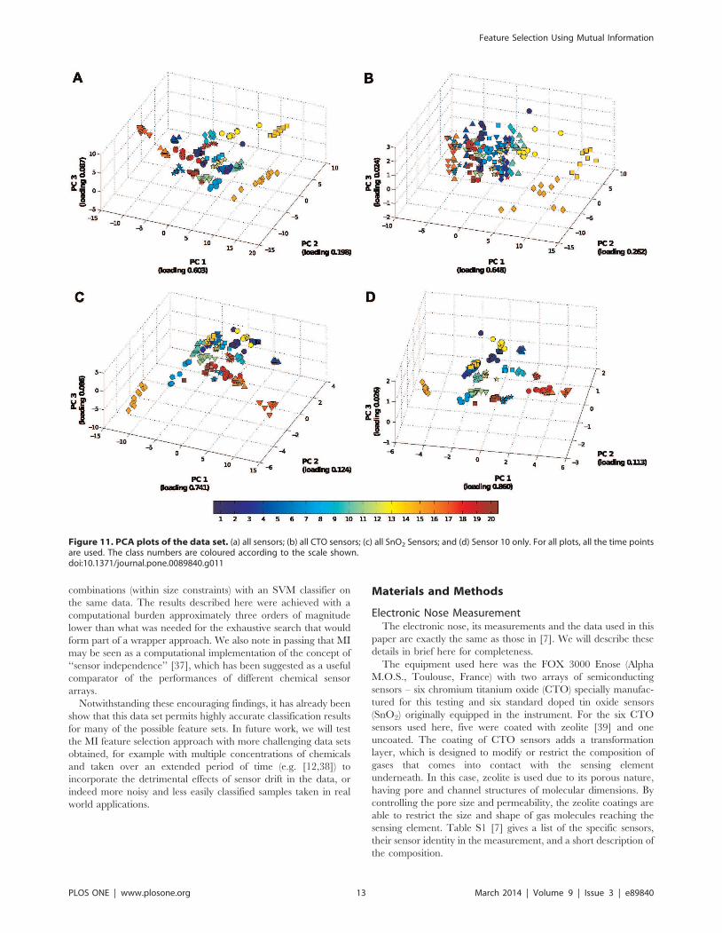
Comparison with PCA AnalysisFigure 11 shows the first three principle components of the data

set for all sensors, for the CTO sensors only, for SnO2 sensors

only, and for data from sensor 10 only, which is the sensor with

very high MI with the classes (Figure 10). The principle

components were calculated based on the covariance matrix of

the data. The PCA plots agree in principle with the frequency of

appearance of sensors in Figure 2, that is, the SnO2 sensors have

better discrimination capability on this data set than the CTO

sensors. There are several reasons for this discrepancy in

classification: Firstly, as Figure 3 shows, the absolute response of

CTO sensors (maximum around 0.2) are a lot lower than the

SnO2 sensors (maximum around 0.9). The responses of CTO

sensors with coating (sensors 2–5, Table S1) are in general lower

than 0.1, which is close to the natural response of the sensors to

dry zero grade air used as a carrier gas for the chemical samples

and recovering phase (see Methods). Secondly, the CTO sensors

were not specially made to respond to these particular chemicals,

while the SnO2 sensors do have the capability for detecting a large

range of organic chemicals (see Table S2).

Further, comparing the PCA plots of all sensors and the SnO2

sensors, we see that the first three principle components of the data

using all the sensors forms better clusterings than those using SnO2

sensors only. This also confirms the finding in Figure 2 and

Table 1, where a combination of sensors from both types is often

selected in the feature sets. Lastly, the PCA plot of the data using

sensor 10 only, agrees with the high MI result of Figure 10 and the

frequent appearance of the sensor in the selected feature sets in

Figure 2A because even though this is using only one sensor, the

classes are still reasonably separated.

Conclusion

We approached the problem of feature selection for arrays of

metal oxide sensors in classification with constraints on the

combination of number of sensors and time points for each feature

set by using a filter approach to maximise the mutual information

among the selected features and the class (identity of chemicals).

We found that our method allows us to discover features that give

consistently better classification performances than randomly

selected features across all the classifiers tested. Furthermore, the

classification performance was not significantly different from that

previously observed in an exhaustive search of all possible feature

Figure 10. Mutual information (MI) between individual features and the class. Note that sensors 1–6 were CTO sensors and 7–12 wereSnO2 sensors.doi:10.1371/journal.pone.0089840.g010



combinations (within size constraints) with an SVM classifier on

the same data. The results described here were achieved with a

computational burden approximately three orders of magnitude

lower than what was needed for the exhaustive search that would

form part of a wrapper approach. We also note in passing that MI

may be seen as a computational implementation of the concept of

‘‘sensor independence’’ [37], which has been suggested as a useful

comparator of the performances of different chemical sensor

arrays.

Notwithstanding these encouraging findings, it has already been

show that this data set permits highly accurate classification results

for many of the possible feature sets. In future work, we will test

the MI feature selection approach with more challenging data sets

obtained, for example with multiple concentrations of chemicals

and taken over an extended period of time (e.g. [12,38]) to

incorporate the detrimental effects of sensor drift in the data, or

indeed more noisy and less easily classified samples taken in real

world applications.

Materials and Methods

Electronic Nose MeasurementThe electronic nose, its measurements and the data used in this

paper are exactly the same as those in [7]. We will describe these

details in brief here for completeness.

The equipment used here was the FOX 3000 Enose (Alpha

M.O.S., Toulouse, France) with two arrays of semiconducting

sensors – six chromium titanium oxide (CTO) specially manufac-

tured for this testing and six standard doped tin oxide sensors

(SnO2) originally equipped in the instrument. For the six CTO

sensors used here, five were coated with zeolite [39] and one

uncoated. The coating of CTO sensors adds a transformation

layer, which is designed to modify or restrict the composition of

gases that comes into contact with the sensing element

underneath. In this case, zeolite is used due to its porous nature,

having pore and channel structures of molecular dimensions. By

controlling the pore size and permeability, the zeolite coatings are

able to restrict the size and shape of gas molecules reaching the

sensing element. Table S1 [7] gives a list of the specific sensors,

their sensor identity in the measurement, and a short description of

the composition.

Figure 11. PCA plots of the data set. (a) all sensors; (b) all CTO sensors; (c) all SnO2 Sensors; and (d) Sensor 10 only. For all plots, all the time pointsare used. The class numbers are coloured according to the scale shown.doi:10.1371/journal.pone.0089840.g011



Twenty different chemical compounds (classes) were analysed

using the FOX eNose. The compounds are from four chemical

groups: alcohols, aldehydes, esters and ketones, each with five

chemicals (see Table S2 for details). The chemicals were chosen

from a large set of chemicals used in a comparison of metal oxide

with biological sensors [37]. Each sample was diluted using

paraffin oil to give final concentrations in the range of 1:22 and

8:03|10{5 M (Table S2). For each chemical, 10 replicates of the

samples were prepared, giving us a total of 200 samples analysed.

The chemical samples were analysed over 4 days. Samples of

1 ml were presented in a 20 ml glass vial using the static

headspace method. The instrument was equipped with an

autosampler (HS50, CTC Analytics, Switzerland), which allows

reproducible injections. The headspace volume of 500 ml of each

sample was taken for analysis, and samples were analysed in

groups based on chemical family. Dry zero grade air was used to

sweep the sample through two chambers housing the different

types of sensors. For each sample, the sensor records 300 s worth

of data at 2 Hz. The instrument is then flushed with zero grade air

for 240 s to allow the sensors to return to baseline. Figure 3 shows

the response of the sensors towards a chemical compound. The

data were captured and pre-analysed using AlphaSoft v.8

(Toulouse, France). (See Dataset S1 for full data set.)

Feature SetThe full feature set used in this paper is also the same as those in

[7]: For each sensor, 6 candidate time points were extracted, those

were: 10, 20, 30, 40, 50 and 60 seconds (cf. Figure 3) from the full

data taken over 300 seconds at 2 Hz. Therefore, the full feature

sets comprised of these 6 time points from each of the 12 sensors.

This gives 212|26 total permutations of combined sensors and

time points. For example, for 6 sensors and 3 time points, there are

12

6

� �

|6

3

� �

~18480 combinations.

Cross-validationAll results reported were obtained from 10-fold balanced cross-

validation as described in [7]. The full data set was partitioned into

training and test sets by randomly selecting 10% of the

measurements from each chemical to form the test set, and the

remaining to form the training set. This process was performed ten

times, where each data sample appears exactly once in a test set.

We then repeat this entire procedure ten times to gather 100 test

(and their corresponding training) sets.

Optimal Feature SelectionThe optimal feature selection task is to select a subset of

features, n(f1,2, . . . ,mg, where m is the total number of features,

such that the resulting subset of features gives the best classification

performance for the given size constraint n on the number of

features in n. We select the subset of features by maximising the

mutual information I(Zn,C) [30] between the selected features

Zn~fZi1 , . . . ,Zing and class C:

I(Zn,C)~X

Zn,C

p(Zn,C) log2p(CDZn)

p(C): ð1Þ

This approach was suggested by Battiti [31], since it minimises the

uncertainty (entropy) H(CDZn) about the class given the features.

MI is increased with the independence of information that the

features contain about the class (similar to the concept of ‘‘sensor

independence’’ in [37]). However, the MI between feature and

class is increased by only the component of independence of the

features which is relevant to the class. That is, MI is not increased

where features contain redundant information about the class.

Furthermore, MI captures the synergies between the features, that

is, what multiple features when considered together (but not

separately) can reveal about the class. Further discussion of the

nature of redundancy and synergy in MI can be found in [40]. A

subtle point is that maximising MI does not mean eliminating all

redundancies between the features — it does mean any

redundancies in the features about the class are not double-counted,

and any features which carry redundancies are only selected due

to unique and synergistic information they provide.

Ordinarily we would evaluate I(Zn,C) for alln

m

� �

combina-

tions of Zn for a given number m of features. Whilst this is

inefficient, and there are alternatives to evaluating all combina-

tions (e.g. the greedy forward feature selection approach described

by Battiti [31]), evaluating all combinations here allows us to

evaluate the features selected by mutual information against all

possible feature selections. Also, note that in this paper our feature

selection is not constrained simply to a subset of size m of the total

number of features, but to select m~S|D features, where S is a

given number of sensors, D is the number of data points

(measurements in time) per sensor and the same D times must

be selected for each sensor. This means we have12

S

� �

|6

D

� �

combinations of features to evaluate.

Another challenge in evaluating Equation 1 here is to estimate

the multivariate joint and conditional density functions for a small

data set (N~180 for each training set). Early approaches tried to

get around the issue by using pairwise approaches (e.g. by Battiti

[31], and the mRMR [34] and QPFS [35] methods). However,

pairwise approaches are effectively heuristics; they do not directly

remove redundancies between features about the class specifically,

and they provide no mechanism to capture synergistic information

provided by multiple features about the class. Other possibilities to

act against small data set size include adaptive forward feature

selection, e.g. [33], which we will investigate in later work. In this

paper, we employed the Kraskov-Grassberger technique [36]

(estimator 2) for estimating the the mutual information. This

technique uses dynamic kernel widths and bias correction, which

provide robustness against small data size. The code used for the

estimation is the publicly available Java Information Dynamics

Toolkit [41].

Classification MethodsWe used several common classifiers to evaluate the effectiveness

of the optimal feature selection.

A support vector machine (SVM) [42] constructs a

hyperplane to separate training data in different classes. We used

the libsvm library [43] to perform the classification using C-SVC

(SVM classification with cost parameter of C). Nine C values,

starting with 1 and increasing by a factor of 4 for each subsequent

value, were tested (i.e. C~f1,4,16,64,256,1024,4096,16384,65536g) to capture the classifier’s performance over large range

of C values. Two types of SVM were used: linear and a nonlinear

SVM using Gaussian radial basis kernel function. The Gaussian

radial basis kernel function is, k(xi,xj)~exp({cExi{xjE2),

where xi is the vector of the data for sample i and c is the kernel

width. We selected c in two ways: the inverse of number of features

(the default c value in libsvm) and the inverse of the 0.1, 0.9

quantile and the median of pairwise distances of the data (See

Figures S2, S3, S4 for the distribution of pairwise distances, and



Figure S5 for a comparison between the two measures). We found

in all cases, C~65536 performs better than or consistently with

the other C values (Figures S1, S6, S7, S8, S9, S10, S11, S12).

Moreover, we found consistent performances between linear SVM

and radial SVM with c~1=n, both better than the classification

performances of radial SVM with other c values (Figure S13).

Therefore, we use the classification performance of linear SVM

with C~65536 in comparison with the other classifiers. To ensure

that this result is optimal, we further performed linear SVM with

C~262144 (i.e. another 4 fold increase on the final C value) and

found this does not improve the classification performance (Figure

S1).

The k nearest neighbour (kNN) algorithm compares the

input data with an existing set of training data by computing a

distance metric [44]. The neighbours of the input data are the k

data points with the smallest distance metric. The input data’s class

is determined to be that with the most data points in the

neighbourhood. In this paper, we used k~9, this is the number of

data samples each class has in the training set, thus the most any

class can appear in the neighbourhood of the input data.

In Bayesian Networks (BN) [45], each node represents a

random variable (these could be observed data or latent variables),

X , with associated probability functions, p(X ). The nodes in a BN

are linked by directed edges which indicate the conditional

dependency between the variables, for example, if the nodes X1

and X2 in a BN are linked by a directed edge from X1 to X2, then

X2 is dependent on X1 and X1 is the parent node to X2. Lastly, the

network as a whole is acyclic. We used the BNT toolbox [46] to

implement the network and perform the classifications. Three

network structures were implemented, a Naıve Bayes Network

where a node representing the class of the chemicals is parent to all

other nodes each of which represents a feature, and two other

networks which are modifications on the Naıve Bayes Network.

The modified networks are: (a) each node, Xi,j , represents a feature

and has parents (i.e. it is dependent on) the nodes Xi{1,j and

Xi,j{1, where i~f1, . . . ,12g is the sensor number and

j~f1, . . . ,6g is the time point number as described in subsection

on Feature Set; (b) each node Xj represents all sensors at time

point j and has parent the node Xj{1. In all three networks, only

the features selected by the MI measure were included in the

network. We found the Naıve Bayes networks performs not as well

as the modified networks, but there is no significant difference

between the performances of the modified networks. We report

here results from the modified network where each node

represents a feature. The sensor numbers for this modified

network were those shown in Table S1 and Figure 3.

An artificial Neural Network (NN) [47] consists of a group of

nodes, or neurons, that are interconnected. We used here a

feedforward NN called multilayer perceptron (MLP) to map the

feature data (input neurons) onto the chemical classes (output

neurons) through two layers of hidden neurons. The MLP was

implemented using the Netlab toolbox [48] with maximum of 100

iterations using three optimisation algorithms (quasi-Newton,

conjugate gradients, and scaled conjugate gradients) and 6 or 12

hidden nodes. We report here results from MLP with 12 hidden

neurons using quasi-Newton optimisation, which performed

slightly better than the others.

Mutual Information maximum likelihood makes a

classification as the class c which maximises the local or pointwise

mutual information I(Zn~z

n,C~c) with the observed (selected)

features, where the pointwise mutual information is

I(Zn~z

n,C~c)~ log2p(znDc)

p(zn)[49]. This approach is equivalent

to selecting the class which maximises the probability p(znDc) of the

observation given the class, and is also equivalent to a classic

maximum likelihood classifier (maximising the posterior p(cDzn))

under the assumption of the marginal distribution for each class

p(c) being equiprobable [50]. The mutual information here was

evaluated using Kraskov-Grassberger estimation [36] (i.e. we do

not assume a multivariate normal distribution here), using the Java

Information Dynamics Toolkit [41].

Hypothesis TestThe two-sided student’s t-test is used to test the null hypothesis

that there is no difference between the classification performance

of two classifiers or two sets of data. When the hypothesis is true

and the population is normal, the test statistic t~�xx{m0

s

ffiffiffi

np

has

the Student’s t distribution with n{1 degrees of freedom (i.e.

t*tn{1), where �xx and s are the mean and standard deviation of

the classification performance of features selected by MI criterion,

m0 is the mean of performance using randomly selected features,

and n~10 is the number of repeats of ten-fold cross-validation

performed. The p-value (for two-sided test) is [51]:

P~2P tn{1§�xx{m0

s

ffiffiffi

np� �

: ð2Þ

Supporting Information

Figure S1 Average classification performance for all the

test sets using linear SVM with different cost values. The

x-axis shows the sensor size constraints used in the feature

selection, each tick mark represents the time point size constraint

of 1, the performance values as marked out on the plots between

two x-axis tick marks represents time point size constraints

f2, . . . ,6g. The y-axis shows the performance in a highly non-

linear, logarithmic scale.

(TIF)

Figure S2 Histogram of 0.1 quantiles of the distribution

of pairwise distance for all possible feature choices.

(TIF)

Figure S3 Histogram of median of the distribution of

pairwise distance for all possible feature choices.

(TIF)

Figure S4 Histogram of 0.9 quantiles of the distribution

of pairwise distance for all possible feature choices.

(TIF)

Figure S5 Comparison of inverse of number of features

and the median pairwise distances for all possible

feature choices.

(TIF)

Figure S6 Average classification performance for all the

test sets using radial SVM with different cost values and

c~1=n, where n is the number of features, for the kernel

function. The x-axis shows the sensor size constraints used in the

feature selection, each tick mark represents the time point size

constraint of 1, the performance values as marked out on the plots

between two x-axis tick marks represents time point size

constraints f2, . . . ,6g. The y-axis shows the performance in a

highly non-linear, logarithmic scale.

(TIF)



Figure S7 Average classification performance for all thetest sets using radial SVM with different cost values andc~0:8 for the kernel function. The c value used here is the

inverse of the average of 0.9 quantile of all the pairwise distance of

the data. The x-axis shows the sensor size constraints used in the






(TIF)

Figure S8 Average classification performance for all thetest sets using radial SVM with different cost values andc~1=d, where d is the 0.9 quantile of the pairwisedistance of the given feature set size, for the kernelfunction. The x-axis shows the sensor size constraints used in the






(TIF)

Figure S9 Average classification performance for all thetest sets using radial SVM with different cost values andc~1:95 for the kernel function. The c value used here is the








(TIF)

Figure S10 Average classification performance for allthe test sets using radial SVM with different cost valuesand c~1=d, where d is the 0.5 quantile of the pairwisedistance of the given feature set size, for the kernelfunction. The x-axis shows the sensor size constraints used in the






(TIF)

Figure S11 Average classification performance for allthe test sets using radial SVM with different cost valuesand c~5 for the kernel function. The c value used here is the








(TIF)

Figure S12 Average classification performance for all

the test sets using radial SVM with different cost values

and c~1=d, where d is the 0.1 quantile of the pairwise

distance of the given feature set size, for the kernel







(TIF)

Figure S13 Comparison of average classification per-

formance for all the test sets using linear SVM and

radial SVM with different c values for the kernel

function. The cost value is set at C~65536, which is the C

value with the best performance for each individual kernel







(TIF)

Table S1 Overview of the sensors used in the electronic

nose. A short description of the sensors is given here. CTO -

Chromium-titanium oxide, SnO2 - Tin Oxide.

(PDF)

Table S2 Chemical compounds analysed. The chemical

are shown here under their group names and corresponding

concentration.

(PDF)

Acknowledgments

We would like to thank CSIRO Advanced Scientific Computing (http://

www.hpsc.csiro.au) for the use of their supercomputer clusters in

performing the experiments for this paper. We would also like to thank

Dr Russell Binions from the School of Engineering and Materials Science

at Queen Mary, University of London for manufacturing the zeolite

sensors for FOX.

Author Contributions

Conceived and designed the experiments: XRW MP. Performed the

experiments: XRW. Analyzed the data: XRW JTL TN. Contributed

reagents/materials/analysis tools: XRW JTL TN AZB. Wrote the paper:

XRW JTL TN SCT.

References

1. Olsson L, Nehaniv CL, Polani D (2004) Information trade-offs and the evolution

of sensory layout. In: Proceedings of the Ninth Int. Conf. on Artificial Life. pp.

119–124.

2. Pashami S, Lilienthal AJ, Trincavelli M (2012) Detecting changes of a distant gas

source with an array of mox gas sensors. Sensors 12: 16404–16419.

3. Martınez S, Bullo F (2006) Optimal sensor placement and motion coordination

for target tracking. Automatica 42: 661–668.

4. Nelson B, Khosla PK (1994) Integrating sensor placement and visual tracking

strategies. In: Yoshikawa T, Miyazaki F, editors, Experimental Robotics III,

volume 200 of Lecture Notes in Control and Information Sciences. Berlin:

Springer. pp. 167–181. doi:10.1007/BFb0027593. Available: http://dx.doi.org/

10.1007/BFb0027593.

5. Zheng H, Zhang Y (2008) Feature selection for high-dimensional data in

astronomy. Advances in Space Research 41: 1960–1964.

6. Saeys Y, Inza I, Larranaga P (2007) A review of feature selection techniques in

bioinformatics. Bioinformatics 23: 2507–2517.

7. Nowotny T, Berna AZ, Binions R, Trowell S (2013) Optimal feature selection

for classifying a large set of chemicals using metal oxide sensors. Sensors and

Actuators B: Chemical 187: 471–480.

8. Marco S, Gutierrez-Galvez A (2012) Signal and data processing for machine

olfaction and chemical sensing: A review. Sensors Journal, IEEE 12: 3189–3214.



http://www.hpsc.csiro.au

http://www.hpsc.csiro.au

http://dx.doi.org/10.1007/BFb0027593

http://dx.doi.org/10.1007/BFb0027593

9. Koinuma H, Takeuchi I (2004) Combinatorial solid-state chemistry of inorganicmaterials. Nature materials 3: 429–38.

10. Dacres H, Wang J, Leitch V, Horne I, Anderson AR, et al. (2011) Greatlyenhanced detection of a volatile ligand at femtomolar levels using biolumines-cence resonance energy transfer (BRET). Biosensors & bioelectronics 29: 119–24.

11. Vergara A, Llobet E (2012) Sensor selection and chemo-sensory optimization:toward an adaptable chemo-sensory system. Frontiers in Neuroengineering 4.

12. Rodriguez-Lujan I, Fonollosa J, Vergara A, Homer M, Huerta R (2014) On thecalibration of sensor arrays for pattern recognition using the minimal number ofexperiments. Chemometrics and Intelligent Laboratory Systems 130: 123–134.

13. Vergara A, Llobet E, Brezmes J, Ivanov P, Cane C, et al. (2007) Quantitative gasmixture analysis using temperature-modulated micro-hotplate gas sensors:Selection and validation of the optimal modulating frequencies. Sensors andActuators B: Chemical 123: 1002–1016.

14. Krause A, Singh A, Guestrin C (2008) Near-optimal sensor placements ingaussian processes: Theory, efficient algorithms and empirical studies. J MachLearn Res 9: 235–284.

15. Gardner J, Boilot P, Hines E (2005) Enhancing electronic nose performance bysensor selection using a new integer-based genetic algorithm approach. Sensorsand Actuators B: Chemical 106: 114–121.

16. Pardo M, Kwong L, Sberveglieri G, Brubaker K, Schneider J, et al. (2005) Dataanalysis for a hybrid sensor array. Sensors and Actuators B: Chemical 106: 136–143.

17. Pardo M, Sberveglieri G (2007) Comparing the performance of different featuresin sensor arrays. Sensors and Actuators B: Chemical 123: 437–443.

18. Guyon I, Elisseeff A (2003) An introduction to variable and feature selection.The Journal of Machine Learning Research 3: 1157–1182.

19. Breiman L, Friedman JH, Olshen RA, Stone CJ (1984) Classification andregression trees. London: Chapman and Hall/CRC. 368 p.

20. Rakotomamonjy A (2003) Variable selection using svm based criteria. TheJournal of Machine Learning Research 3: 1357–1370.

21. Raman B, Meier DC, Evju JK, Semancik S (2009) Designing and optimizingmicrosensor arrays for recognizing chemical hazards in complex environments.Sensors and Actuators B: Chemical 137: 617–629.

22. Muezzinoglu MK, Vergara A, Huerta R, Rabinovich MI (2010) A sensorconditioning principle for odor identification. Sensors and Actuators B:Chemical 146: 472–476.

23. Llobet E, Brezmes J, Gualdron O, Vilanova X, Correig X (2004) Buildingparsimonious fuzzy ARTMAP models by variable selection with a cascadedgenetic algorithm: application to multisensor systems for gas analysis. Sensorsand Actuators B: Chemical 99: 267–272.

24. Aleixandre M, Sayago I, Horrillo M, Fernandez M, Ares L, et al. (2004) Analysisof neural networks and analysis of feature selection with genetic algorithm todiscriminate among pollutant gas. Sensors and Actuators B: Chemical 103: 122–128.

25. Shannon CE (1948) A mathematical theory of communication. The Bell SystemTechnical Journal 27: 379–423, 623–656, July, October.

26. Guestrin C, Krause A, Singh A (2005) Near-optimal sensor placements inGaussian processes. In: Int. Conf. on Machine Learning. pp. 265–272.

27. Wang XR, Mathews G, Price D, Prokopenko M (2009) Optimising sensorlayouts for direct measurement of discrete variables. In: Self-Adaptive and Self-Organizing Systems, 2009. SASO’09. Third IEEE International Conference on.pp. 92–102.

28. Pearce TC, Sanchez-Montanes MA (2004) Chemical Sensor Array Optimiza-tion: Geometric and Information Theoretic Approaches. Weinheim, Germany:Wiley-VCH Verlag GmbH & Co. KGaA. pp. 347–375. doi: 10.1002/3527601597.ch14. Available: http://dx.doi.org/10.1002/3527601597.ch14.

29. Vergara A, Muezzinoglu MK, Rulkov N, Huerta R (2010) Information-theoreticoptimization of chemical sensors. Sensors and Actuators B: Chemical 148: 298–306.

30. Cover TM, Thomas JA (1991) Elements of Information Theory. New York:Wiley-Interscience.

31. Battiti R (1994) Using mutual information for selecting features in supervisedneural net learning. IEEE Trans Neural Networks 5: 537–550.

32. Fonollosa J, Fernandez L, Huerta R, Gutierrez-Galvez A, Marco S (2013)Temperature optimization of metal oxide sensor arrays using mutualinformation. Sensors and Actuators B: Chemical 187: 331–339.

33. Avdiyenko L, Bertschinger N, Jost J (2012) Adaptive sequential feature selectionfor pattern classification. In: Proceedings of the 4th International Conference onNeural Computation Theory and Applications (NCTA 2012), part of theInternational Joint Conference of Computational Intelligence (IJCCI). Barce-lona, Spain, pp. 474–482.

34. Peng H, Long F, Ding C (2005) Feature selection based on mutual information:criteria of maxdependency, max-relevance, and min-redundancy. IEEETransactions on Pattern Analysis and Machine Intelligence 27: 1226–1238.

35. Rodriguez-Lujan I, Huerta R, Elkan C, Cruz CS (2010) Quadraticprogramming feature selection. Journal of Machine Learning Research 99:1491–1516.

36. Kraskov A, Stogbauer H, Grassberger P (2004) Estimating mutual information.Physical Review E 69: 066138+.

37. Berna AZ, Anderson AR, Trowell SC (2009) Bio-benchmarking of electronicnose sensors. PLoS ONE 4: e6406.

38. Vergara A, Vembu S, Ayhan T, Ryan MA, Homer ML, et al. (2012) Chemicalgas sensor drift compensation using classifier ensembles. Sensors and ActuatorsB: Chemical 166167: 320–329.

39. Binions R, Davies H, Afonja A, Dungey S, Lewis D, et al. (2009) Zeolite-modified discriminating gas sensors. Journal of The Electrochemical Society156: J46–J51.

40. Williams PL, Beer RD (2010) Nonnegative decomposition of multivariateinformation. CoRR abs/1004.2515.

41. Lizier JT (2012) JIDT: An information-theoretic toolkit for studying thedynamics of complex systems. Available: https://code.google.com/p/information-dynamics-toolkit/. Accessed 2014 Feb 11.

42. Cortes C, Vapnik V (1995) Support-vector networks. Machine Learning 20:273–297.

43. Chang CC, Lin CJ (2011) LIBSVM: A library for support vector machines.ACM Transactions on Intelligent Systems and Technology 2: 27:1–27:27.

44. Russell S, Norvig P (1995) Artificial Intelligence: A Modern Approach.Englewood Cliffs, NJ: Prentice Hall.

45. Friedman N, Geiger D, Goldszmidt M (1997) Bayesian Network classifiers.Machine Learning 29: 131–163.

46. Murphy K (2001) The bayes net toolbox for matlab. In: Wegman EJ, BravermanA, Goodman A, Smyth P, editors. Computing Science and Statistics, vol. 33.Fairfax Station, VA: Interface Foundation of North America, Inc. pp. 331–350.

47. Bishop CM (1995) Neural Networks for Pattern Recognition. Oxford: OxfordUniversity Press.

48. Nabney I (2002) Netlab: Algorithms for Pattern Recognition. Advances inPattern Recognition. Berlin: Springer.

49. Fano RM (1961) Transmission of information: a statistical theory ofcommunications. Cambridge, MA: MIT Press.

50. Myung IJ (2003) Tutorial on maximum likelihood estimation. J Math Psychol47: 90–100.

51. Phipps MC, Quine MP (1998) A Primer of Statistics: data analysis, probability,inference. Brisbane, QLD: Prentice Hall Australia.



http://dx.doi.org/10.1002/3527601597.ch14

https://code.google.com/p/information-dynamics-toolkit/

https://code.google.com/p/information-dynamics-toolkit/

feature selection for chemical sensor arrays using mutual...

Documents